interim report ir-09-24 overview of methods implemented in

International Institute for Tel: 43 2236 807 342Applied Systems Analysis Fax: 43 2236 71313Schlossplatz 1 E-mail: [email protected] Laxenburg, Austria Web: www.iiasa.ac.at

Interim Report IR-09-24

Overview of Methods Implemented in MCA:Multiple Criteria Analysis of Discrete Alternativeswith a Simple Preference SpecificationMarek Makowski ([email protected])Janusz Granat ([email protected])Włodzimierz Ogryczak ([email protected])

Approved by

Detlof von Winterfeldt ([email protected])Director, IIASA

December 2009

Interim Reports on work of the International Institute for Applied Systems Analysis receive only limitedreview. Views or opinions expressed herein do not necessarily represent those of the Institute, its NationalMember Organizations, or other organizations supporting the work.

M. Makowski, J. Granat, W. Ogryczak - ii - Overview of methods implemented in MCA

Foreword

Practically all important decisions involve analysis of several (or even many), typicallyconflicting, criteria. Analysis of trade-offs between criteria is difficult because such trade-offs for most problems are practically impossible to be defined a-priori even by analystsexperienced in Multi-Criteria Analysis (MCA). Therefore the trade-offs emerge during aninteractive MCA which actually supports a learning process about the trade-offs. Hence,effective MCA methods are important for actual support of decision-making processes,especially those related to policy-making.

IIASA has been developing novel methods for MCA since mid 1970s, and success-fully applying them to many practical problems in various areas of applications. How-ever, there are new practical problems for which the existing MCA methods (developednot only at IIASA but also by many researchers all over the world) are not satisfactory.In particular, discrete decision problems with a large number of criteria and alternatives(the latter making pairwise comparisons by the users impracticable) demand new meth-ods. For example, MCA analysis of future energy technologies involves over 60 criteriaand over 20 discrete alternatives; a careful requirement analysis of this application hasproven that none of the existing MCA methods is suitable for an effective analysis ofthe corresponding problem. Moreover, this analysis has been done by a large number ofstakeholders with diverse backgrounds and preferences; most of them have no analyti-cal skills, therefore the specification of preferences needed to be simple but still provideeffective and intuitive analysis of the Pareto set.

The paper provides an overview of several new methods for MCA of discrete alter-natives that have been implemented in the MCA, the Web-based application for multiplecriteria analysis of discrete alternatives.

M. Makowski, J. Granat, W. Ogryczak - iii - Overview of methods implemented in MCA

Abstract

Many methods have been developed for multiple criteria analysis and/or ranking of dis-crete alternatives. Most of them require complex specification of preferences. Therefore,they are not applicable for problems with numerous alternatives and/or criteria, wherepreference specification by the decision makers can hardly be done in a way acceptablefor small problems, e.g., for pair-wise comparisons.

In this paper we describe several new methods implemented for a real-life applicationdealing with multi-criteria analysis of future energy technologies. This analysis involveslarge numbers of both alternatives and criteria. Moreover, the analysis was made by alarge number of stakeholders without experience in analytical methods. Therefore a sim-ple method for interactive preference specification was a condition for the analysis. Thepaper provides overview of several of new methods based on diverse concepts developedfor multicriteria analysis, and summarizes a comparison of methods and experience ofusing them.

M. Makowski, J. Granat, W. Ogryczak - iv - Overview of methods implemented in MCA

Acknowledgments

The authors gratefully acknowledge the long-term collaboration with, and help of AndrzejP. Wierzbicki of the National Institute of Telecommunications, Warsaw, Poland, who overthree decades greatly influenced the developments of the multiple criteria methodology.The authors also thank Stefan Hirschberg, Peter Burgherr, and Warren W. Schenler, all ofthe Laboratory for Energy Systems Analysis, Paul Scherrer Institute, Villigen, Switzer-land, for the numerous discussions during the over four years collaboration within theNEEDS Project.

The research reported in this paper was partly financially supported by the EC-fundedIntegrated Project NEEDS (project no: 502687), and by the Austrian Federal Ministry ofScience and Research.

M. Makowski, J. Granat, W. Ogryczak - v - Overview of methods implemented in MCA

About the authors

Marek Makowski leads the IIASA Integrated Modeling Environment Project. His re-search interests focus on model-based support for solving complex problems, whichincorporates three interlinked areas. First, integration of interdisciplinary knowl-edge and its representation by mathematical models. Second, creation of knowl-edge by comprehensive model analysis, including multicriteria methods. Third,tailoring the modeling process to meet the needs of decision-making processes.Thus Marek’s research interests cover a cluster of areas relevant to the adaptation(whenever possible) or development (when needed) of methodology, algorithms,and software for model-based decision-making support. This includes more spe-cific topics in Operations Research such as: multicriteria problem analysis, largescale optimization, optimization of badly conditioned problems, use of databasemanagement systems for complex models, decision analysis and support, user in-terfaces in decision support systems, effective treatment of uncertainty and risk.

Marek has published over 130 papers and book-chapters, co-edited four books, co-ordinated or led several scientific projects, and has been twice guest editor of theEuropean Journal of Operational Research.

Janusz Granat is a leader of a Division of Advanced Information Technology at the Na-tional Institute of Telecommunications. He also lectures on decision support sys-tems and management information systems at the Warsaw University of Technol-ogy. His scientific interests include decision support systems, multi-criteria analy-sis, modeling, data mining, event mining, techno-economic analysis and the designof the telecommunications network. He has been involved in various industrial andscientific projects e.g., data warehousing and decision support systems for telecom-munication industry, building data mining models for marketing departments, de-velopment of decision support systems for energy management.

Włodzimierz Ogryczak is a Professor and Deputy Director for Research in the Instituteof Control and Computation Engineering at the Warsaw University of Technology,Poland. His research interests are focused on models, computer solutions and inter-disciplinary applications in the area of optimization and decision making. Withinthese the main stress is on the methodology of multiple criteria optimization and de-cision support, decision making under risk, location and distribution problems. Hehas published three books and numerous research articles in international journals.

M. Makowski, J. Granat, W. Ogryczak - vi - Overview of methods implemented in MCA

Contents

1 Introduction 1

2 Background 1

3 Structure of the multicriteria analysis specification 43.1 Problem specification . . . . . . . . . . . . . . . . . . . . . . . . . . . . 43.2 Instance specification . . . . . . . . . . . . . . . . . . . . . . . . . . . . 5

3.2.1 Hierarchy of criteria . . . . . . . . . . . . . . . . . . . . . . . . 53.3 Analysis specification . . . . . . . . . . . . . . . . . . . . . . . . . . . . 6

4 Specification of preferences 64.1 Required for all methods . . . . . . . . . . . . . . . . . . . . . . . . . . 6

4.1.1 Required for some methods . . . . . . . . . . . . . . . . . . . . 74.1.2 Optional or computed from data . . . . . . . . . . . . . . . . . . 7

5 Representation of preferences in MC solvers 7

6 Objects and functions common for all methods 86.1 Active leaf-criteria . . . . . . . . . . . . . . . . . . . . . . . . . . . . . 86.2 Set of Pareto alternatives . . . . . . . . . . . . . . . . . . . . . . . . . . 96.3 Criteria relative importance . . . . . . . . . . . . . . . . . . . . . . . . . 9

6.3.1 Standard mapping . . . . . . . . . . . . . . . . . . . . . . . . . 96.3.2 Multiplicative mapping . . . . . . . . . . . . . . . . . . . . . . . 106.3.3 Weights for criteria hierarchy . . . . . . . . . . . . . . . . . . . 10

6.4 Individual Achievement Functions . . . . . . . . . . . . . . . . . . . . . 11

7 Auxiliary functions 117.1 Ordered Achievement Functions (OAF) . . . . . . . . . . . . . . . . . . 117.2 PWL functions for Quantile Aggregation . . . . . . . . . . . . . . . . . . 127.3 Aggregated Ordered Achievement Functions (AOAF) . . . . . . . . . . . 12

8 Methods 138.1 Objective Choice (OC) . . . . . . . . . . . . . . . . . . . . . . . . . . . 14

8.1.1 Objective ASP/RES . . . . . . . . . . . . . . . . . . . . . . . . 148.1.2 Achievement Functions . . . . . . . . . . . . . . . . . . . . . . . 148.1.3 Scalarizing Functions . . . . . . . . . . . . . . . . . . . . . . . . 14

8.2 Aspiration-Reservation (AspRes) . . . . . . . . . . . . . . . . . . . . . . 158.3 RFP - Nadir . . . . . . . . . . . . . . . . . . . . . . . . . . . . . . . . . 158.4 RFP - Utopia . . . . . . . . . . . . . . . . . . . . . . . . . . . . . . . . 168.5 RFP - Pareto . . . . . . . . . . . . . . . . . . . . . . . . . . . . . . . . . 17

M. Makowski, J. Granat, W. Ogryczak - vii - Overview of methods implemented in MCA

8.6 Pairwise Outperformance Aggregation (POA) . . . . . . . . . . . . . . . 188.7 Non-linear Aggregation (NA) . . . . . . . . . . . . . . . . . . . . . . . . 198.8 Quantile Aggregation (QA) . . . . . . . . . . . . . . . . . . . . . . . . . 208.9 LexMaxReg . . . . . . . . . . . . . . . . . . . . . . . . . . . . . . . . . 218.10 Weighted Sum (WS) . . . . . . . . . . . . . . . . . . . . . . . . . . . . 21

9 Comparison of selected methods 21

10 Ranking of alternatives 22

11 Other functions of the solvers 2211.1 Preprocessing . . . . . . . . . . . . . . . . . . . . . . . . . . . . . . . . 2211.2 Info provided withthe bestalternative . . . . . . . . . . . . . . . . . . . 2311.3 More info about the MCA . . . . . . . . . . . . . . . . . . . . . . . . . 23

References 24

A Lorenz curve and quantile measures 26

M. Makowski, J. Granat, W. Ogryczak - viii - Overview of methods implemented in MCA

List of Tables

1 Pairwise comparisons of methods. . . . . . . . . . . . . . . . . . . . . . 22

M. Makowski, J. Granat, W. Ogryczak - ix - Overview of methods implemented in MCA

List of Figures

1 Example of criteria hierarchy. . . . . . . . . . . . . . . . . . . . . . . . . 52 Hierarchy of active criteria . . . . . . . . . . . . . . . . . . . . . . . . . 83 Examples of the Aggregated Ordered Achievement FunctionsL1j (15)

for the problem with 4 alternatives and 16 criteria. . . . . . . . . . . . . . 154 Nadir-based RFP method. The improvement direction is defined by the

scaling/weighting vectorw , see eq. (3) or (9). . . . . . . . . . . . . . . . 165 Utopia-based RFP method. The direction is defined by the vectorv , see

eq. (1). . . . . . . . . . . . . . . . . . . . . . . . . . . . . . . . . . . . . 166 RFP-Pareto (not reliable) method. . . . . . . . . . . . . . . . . . . . . . 177 RFP-Pareto method. . . . . . . . . . . . . . . . . . . . . . . . . . . . . . 188 Histogram of the average frequency of the comparison results. . . . . . . 239 Lorenz curve illustrating distribution of household incomes. . . . . . . . 2610 Absolute Lorenz Curves. . . . . . . . . . . . . . . . . . . . . . . . . . . 2711 Lorenz curve for the alternatives presented in Sec. 8.1.1. . . . . . . . . . 2812 Absolute Lorenz Curve and the worst conditional mean. . . . . . . . . . . 2913 WOWA calculation according to formula (54). . . . . . . . . . . . . . . . 30

M. Makowski, J. Granat, W. Ogryczak - 1 - Overview of methods implemented in MCA

Overview of Methods Implemented in MCA:Multiple Criteria Analysis of Discrete Alternatives

with a Simple Preference Specification

Marek Makowski* ([email protected])Janusz Granat** *** ([email protected])

Włodzimierz Ogryczak*** ([email protected])

1 Introduction

The paper has a rather technical character; it provides an overview of several new methodsfor Multiple Criteria Analysis (MCA) of discrete alternatives that have been implementedin the MCA, the Web-based application for multiple criteria analysis of discrete alterna-tives; the user guide and tutorial to the MCA is available in [6].

This report is addressed to advanced users who are interested in general properties ofthe new methods. Detailed presentation of some of these methods and their methodolog-ical background together with several associated concepts, including automated pairwisecomparisons which lead to the corresponding pairwise outperformance aggregations, areprovided in [2].

The structure of the paper is as follows: Section 2 summarizes the background of theMCA, followed by the simple approach to specification of preferences and their represen-tation is solvers described in Section 4 and 5, respectively. The next two Sections providespecifications of objects and functions used in the specifications of methods. The methodsare specified in Section 8. Section 9 summarizes results of comparing the methods. Theremaining two Sections provide auxiliary information, and the Appendix summarizes thebasic information about the Lorenz curve and quantile measures.

2 Background

Multi-Criteria Analysis (MCA) deals with finding optimal (best in the sense of selectedgoal function) solution1 for a problem characterized by a vector of outcomes;2 i.e., the

* Integrated Modeling Environment Project, IIASA.** National Institute of Telecommunications, Warsaw, Poland.

*** Warsaw University of Technology, Warsaw, Poland.1For discrete problems alternatives are usually called alternatives; in this paper we use both terms as

synonyms.2Outcomes are often called attributes, or criteria, or indicators. We use these terms interchangeably, and

also often omit the phrasevector of, i.e., outcomes actually stands for vector of outcomes.


problem can be formulated as a multiple-criteria optimization one. Without a loss of gen-eralization one usually considers maximization of all outcomes. The qualitative differencebetween the classical (single-criterion) optimization and the MCA is that for the formerone it is possible to define an apriori goal function which induces a complete ordering inthe solution space, thus allows for finding an optimal solution.

For a truly multi-criteria problem it is impractical to define such an apriori goal func-tion, therefore there exist alternatives that cannot be ordered (based on a formal compari-son resulting in deciding that solution is better than another one). In many applications itis possible to limit the analysis to a subset of all solutions called thePareto set.3 A solu-tion is called Pareto-efficient, if there is no other solution for which at least one criterionhas a better value while values of remaining criteria are the same or better. In other words,one cannot improve any criterion without worsening at least one other criterion. Solutionsthat are not Pareto efficient are called dominated.

Alternatives belonging to a Pareto set cannot be compared in mathematical sense, i.e.,one cannot objectively decide which one of any two selected from this set is better. How-ever, the user has to eventually select one alternatives at thebestone. The user is usuallyable to make a pair-wise comparison, i.e., subjectively select one of two presented alter-natives as a preferred one. Pair-wise comparisons can be very efficient, if the numbers ofboth alternatives and criteria are very small.4 For non-trivial problems however computer-based support is needed for helping the user to specify preferences in a structured way,and to modify them while learning about attainable trade-offs between the criteria values.The preferences are typically specified in two categories:• a measure of satisfaction level from achieving specific values of each criterion;• information on trade-offs between the satisfaction levels of different criteria.

This document summarizes methodological background and outlines implementationof several MCA methods developed for a specific class of multicriteria analysis of a setof discrete alternatives characterized by:• large number of discrete alternatives (about 20), each defined by about 40 attributes

(some of the attributes having multimodal distribution of values);• large number of criteria (about 60) organized in hierarchical structure (the criteria in-

clude the attributes that define the alternatives);• large number of stakeholders (about 3000) invited for making individual analysis; the

stakeholders have diversified backgrounds, very few of them have knowledge/experienceabout/in multicriteria analysis.

We stress that we deal with multicriteria analysis (as opposed to the commonly usedterm multicriteria decision analysis). This class of problems requires:• development of new MCA methods (see [1] for the justification of this statement), and

also clarification of several methodological issues;• a simple and intuitive interface for specification of user preferences that meets the re-

quirements specified in [7].These both elements may be interesting for a broad audience of researchers and prac-

titioners involved in the MCA.3Also called: Pareto-efficient solutions, Pareto frontier, non-dominated solutions. For the sake of brevity

we don’t deal here with more advanced concepts, e.g., properly efficient solutions; these are discussed e.g.,in [13].

4Note that 15 pair-wise comparisons are needed for 6 alternatives.


In order to help the users to analyze the problem and to find thebestalternative wehave implemented a Web-based interactive iterative procedure composed of the followingsteps:• the user specifies preferences in the criteria space;• the preferences are used for defining an ad-hoc goal function, and applying it for finding

a solution;• the user confronts the criteria values in the found solution with the specified preferences;• the moves to the first step as long as the trade-offs between the found criteria values

differ from the user expectations.Thus we consider MCA as an iterative process composed of iterations. The first it-

eration is generated automatically. Then the user can select any of the iterations (fromthe tree of iterations belonging to his/her analysis composed of the initial iteration, andthe iterations he/she has made) as a basis for creating a new iteration. Upon analysis ofcriteria values for the selected basis iteration the user modifies her/his preferences, andcalls the solver, which provides a Pareto-efficient alternative corresponding best to thespecified preferences.

This typical MCA procedure contains the main challenge for any multicriteria anal-ysis method:how to find a Pareto solution that matches best the user preferences. Thischallenge appears to be even bigger, if the MCA methods are designed and implementedfor users having no experience in mathematical modeling. However, it has been observedthat also users with extensive experience in MCA have problems with a consistent speci-fication of preferences, if such a specification involves a process with several interlinkedsteps.

Specification of preferences for all methods described in this paper is done in theprobably easiest way: by selecting a relative importance of each criterion. The relativeimportance is expressed in qualitative terms, and then the relative importance are mapped(see Section 6.3) into the user defined weights. Note that the weights are normalized,therefore specifying an equal importance for all criteria has the same effect irrespectivelyof the selected importance level.

Thus the user forms a pattern of relative criteria importance, and expects to get aPareto solution (alternative) having the corresponding pattern of criteria values, e.g., pos-sibly best values of all very important criteria, good values for all important criteria, etc.However, usually there is no alternative having criteria values that correspond well to theuser expectations.

The MCA is actually a learning process during which the user modifies his/her pref-erences in order to find an alternative with trade-offs between criteria values that fits bestthe user preferences. In other words, a specification of preferences is a tool for finding apreferred alternative. The preferred means that it has the best (in subjective opinion of theuser) trade-offs of the criteria values amongst all alternatives; this should not be confusedwith the specified trade-offs which are often not attainable (i.e., there exists no alterna-tive having the specified pattern of criteria values). Moreover, it is not really importantwhich pattern of criteria importance led to finding the preferred alternative; actually, eachalternative can be found for many rather different specified preferences.

A good method for MCA shall therefore provide the user with an intuitive way tomodify specification of preferences in order to help the user to find his/her preferred al-ternative. The user preferences are then used as parameters for a selected Scalarizing


Function SF that induces an ad-hoc complete order in the set of Pareto alternatives. Inother words, the SF is defined on vectors of outcomes (characterizing each alternative),and thus assigns a real value for each alternative. Thus any MCA method can be charac-terized by the parameters representing the user preferences, and the corresponding SF (ora procedure used instead of the SF for inducing a complete order in the alternative space).

A SF is actually a way for aggregating the individual outcomes according to the userpreferences. SFs have various forms and properties that correspond on diversified ap-proaches to preference modeling. Nevertheless, most scalarizing functions can be viewedas two-stage transformations of the original outcomes.

First the individual outcomes are rescaled to some uniform measures of achievements;these measures may include some preference parameters. Thus, the role of individualachievement functions is to measure (on a scale common to all criteria) the user sat-isfaction level related to each possible criterion value. This measure does not concernpreferences related to trade-offs between criteria.

In the second stage the individual outcomes transformed into a uniform scale of indi-vidual achievements they are aggregated through a definition of the SF into a final scalar-ization. Different MCA methods use different aggregations (e.g., measuring the total oraverage, or the worst individual achievement). Moreover, the methods differ by one oftwo possible assumptions. The first assumes that the aggregation is impartial or sym-metric with respect to the individual achievements; thus the achievements are treated asequally important. The second approach uses for the aggregation diversified measuresreflecting relative criteria importance.

3 Structure of the multicriteria analysis specification

MCAA is an iterative process, i.e., the user makes a sequence of iterations for a selectedanalysis instance. For efficiency reasons analysis instances are defined in three stages:1. problem specification (Sec. 3.1)2. problem instance specification (Sec. 3.2)3. analysis instance specification (Sec. 3.3)

For each analysis instance (later on calledanalysis) initial iteration is generated au-tomatically. Then the user selects any iteration (from the tree of iterations composed ofthe initial iteration, and the iterations he/she has made), analyses the current trade-offs be-tween criteria, specifies new preferences, and calls a solver. Thus an iteration is composedof:• specified preferences for the criteria (equitable preferences are assumed for the initial

iteration),• the corresponding Pareto solution,• optionally,5 a method chosen for selecting a Pareto solution.

3.1 Problem specification

Multicriteria problem specification is composed of three parts:• attribute names6, indexed byi = 1, . . . , n (also denotedi ∈ I).

5A default method is used, if the user does not select a method.6Attributes are also called indicators or outcomes, or criteria.


• alternative names, indexed byj = 1, . . . ,m (alsoj ∈ J),• attribute values denoted byqij specified for each pair{i, j}

Thus the attribute values are organized in a matrixQ composed of elementsqij. Forconveniencej-th column ofQ (composed of values of all criteria forj-th alternative) isdenoted byqj, andi-th row ofQ (composed of values ofi-th criterion for all alternatives)is denoted byqi.

3.2 Instance specification

Multicriteria problem instance is composed of:• Set of alternatives (selected from the problem specification).• Set of criteria defined using a selected attribute and one of defined types (maximized,

minimized, target7).• Optionally, a hierarchy of criteria (Sec. 3.2.1) can be defined. In such cases, when it is

necessary to distinguish the criteria derived from attributes they are called leaf-criteriaor lowest-level criteria.

3.2.1 Hierarchy of criteria

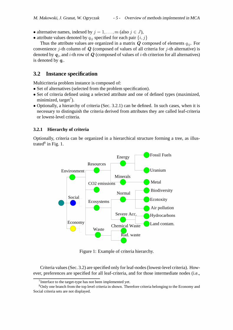
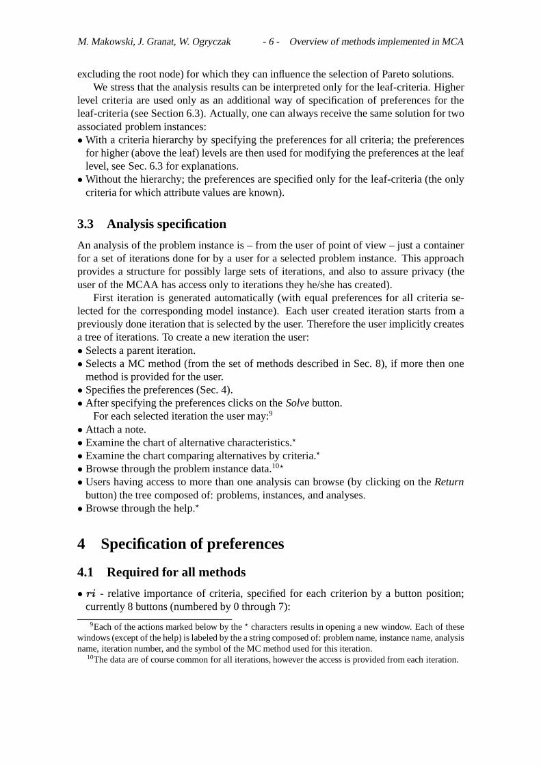
Optionally, criteria can be organized in a hierarchical structure forming a tree, as illus-trated8 in Fig. 1.

Hydrocarbons

Environment

Social

Economy

Rad. waste

Resources

CO2 emissions

Ecosystems

Waste

Energy

Minerals

Normal

Severe Acc.

Chemical Waste

Fossil Fuels

Uranium

Metal

Biodiversity

Ecotoxity

Air pollution

Land contam.

Figure 1: Example of criteria hierarchy.

Criteria values (Sec. 3.2) are specified only for leaf-nodes (lowest-level criteria). How-ever, preferences are specified for all leaf-criteria, and for those intermediate nodes (i.e.,

7Interface to the target-type has not been implemented yet.8Only one branch from the top level criteria in shown. Therefore criteria belonging to the Economy and

Social criteria sets are not displayed.


excluding the root node) for which they can influence the selection of Pareto solutions.We stress that the analysis results can be interpreted only for the leaf-criteria. Higher

level criteria are used only as an additional way of specification of preferences for theleaf-criteria (see Section 6.3). Actually, one can always receive the same solution for twoassociated problem instances:•With a criteria hierarchy by specifying the preferences for all criteria; the preferences

for higher (above the leaf) levels are then used for modifying the preferences at the leaflevel, see Sec. 6.3 for explanations.•Without the hierarchy; the preferences are specified only for the leaf-criteria (the only

criteria for which attribute values are known).

3.3 Analysis specification

An analysis of the problem instance is – from the user of point of view – just a containerfor a set of iterations done for by a user for a selected problem instance. This approachprovides a structure for possibly large sets of iterations, and also to assure privacy (theuser of the MCAA has access only to iterations they he/she has created).

First iteration is generated automatically (with equal preferences for all criteria se-lected for the corresponding model instance). Each user created iteration starts from apreviously done iteration that is selected by the user. Therefore the user implicitly createsa tree of iterations. To create a new iteration the user:• Selects a parent iteration.• Selects a MC method (from the set of methods described in Sec. 8), if more then one

method is provided for the user.• Specifies the preferences (Sec. 4).• After specifying the preferences clicks on theSolvebutton.

For each selected iteration the user may:9

• Attach a note.• Examine the chart of alternative characteristics.?

• Examine the chart comparing alternatives by criteria.?

• Browse through the problem instance data.10?

• Users having access to more than one analysis can browse (by clicking on theReturnbutton) the tree composed of: problems, instances, and analyses.• Browse through the help.?

4 Specification of preferences

4.1 Required for all methods

• ri - relative importance of criteria, specified for each criterion by a button position;currently 8 buttons (numbered by 0 through 7):

9Each of the actions marked below by the? characters results in opening a new window. Each of thesewindows (except of the help) is labeled by the a string composed of: problem name, instance name, analysisname, iteration number, and the symbol of the MC method used for this iteration.

10The data are of course common for all iterations, however the access is provided from each iteration.


? 0-th button: ignore the criterion;Note:criteria ”below” (i.e., children, grandchildren, . . . ) ignored criteria are assumedto be also ignored (therefore solvers redefine the specified values of correspondingriito 0).

? 4-th button: average importance;? buttons 5 through 7: more, much more, vastly more, important than average, respec-

tively;? buttons 3 through 1: less, much less, vastly less, important than average, respectively;

4.1.1 Required for some methods

• impr - selection of criteria that shall be improved and those to be compromised; thisis specified for each criterion by a button position; currently 4 buttons (numbered by 0through 3):? 0th button: allow to compromise (worsen) the criterion value;? 1st button: free the criterion (change in any direction);? 2nd button: stabilize the criterion value (preference for keeping changes small);? 3rd button: improve the criterion value;

4.1.2 Optional or computed from data

• res reservation andasp aspiration values for each criterion• rfp reference point (one value for each criterion)

5 Representation of preferences in MC solvers

The preferences are specified for each iteration (except of the initial one). First, the useroptionally selects for each iteration the method which will be used to find a Pareto solutionthat fits best his/her preferences. The way the preferences are specified depends on themethod so advanced users may experiment with different methods and find the favoriteone. Each method uses the associated solver. The methods/solvers differ by the internalrepresentation of user preferences, and the way in which a Pareto solution is selected forspecific preferences. However, several elements of solvers are common, and are thereforepresented before each method will be outlined with method-specific elements.

All methods use the following six11 types of objects and corresponding functions:• selection of active leaf-criteria• selection of Pareto alternatives• wi(ri) andvi(wi) - criteria scaling/weighting;• IAi(qi) - Individual Achievement functions measuring (for each criterion separately)

the satisfaction level corresponding to a value of the criterion;• AFi(w , v , IA) - Achievement Function measuring (for each criterion) the satisfaction

level corresponding to a value of the criterion taking into account relative importance(represented bywi(ri) or/andvi(wi)) of all criteria;• SF (AF) - Scalarizing Function measuring satisfaction levels for each alternative.

11We present here only a subset of solver elements that are necessary for understanding the methodsused.


The first four are common for all methods, while the other two are specific for amethod (or a set of methods). For the latter some auxiliary functions or relations aredefined later. Therefore we first (Sec. 6) define the common functions, and then (Sec. 8)introduce methods, each of the latter accompanying with the corresponding definitions ofAF(·) andSF(·).

6 Objects and functions common for all methods

6.1 Active leaf-criteria

Hydrocarbons

��

��

��

��

��

��

��

��

��

��

��

��

��

��

Environment

Social

Economy

Rad. waste

Resources

CO2 emissions

Ecosystems

Waste

Energy

Minerals

Normal

Severe Acc.

Chemical Waste

Fossil Fuels

Uranium

Metal

Biodiversity

Ecotoxity

Air pollution

Land contam.

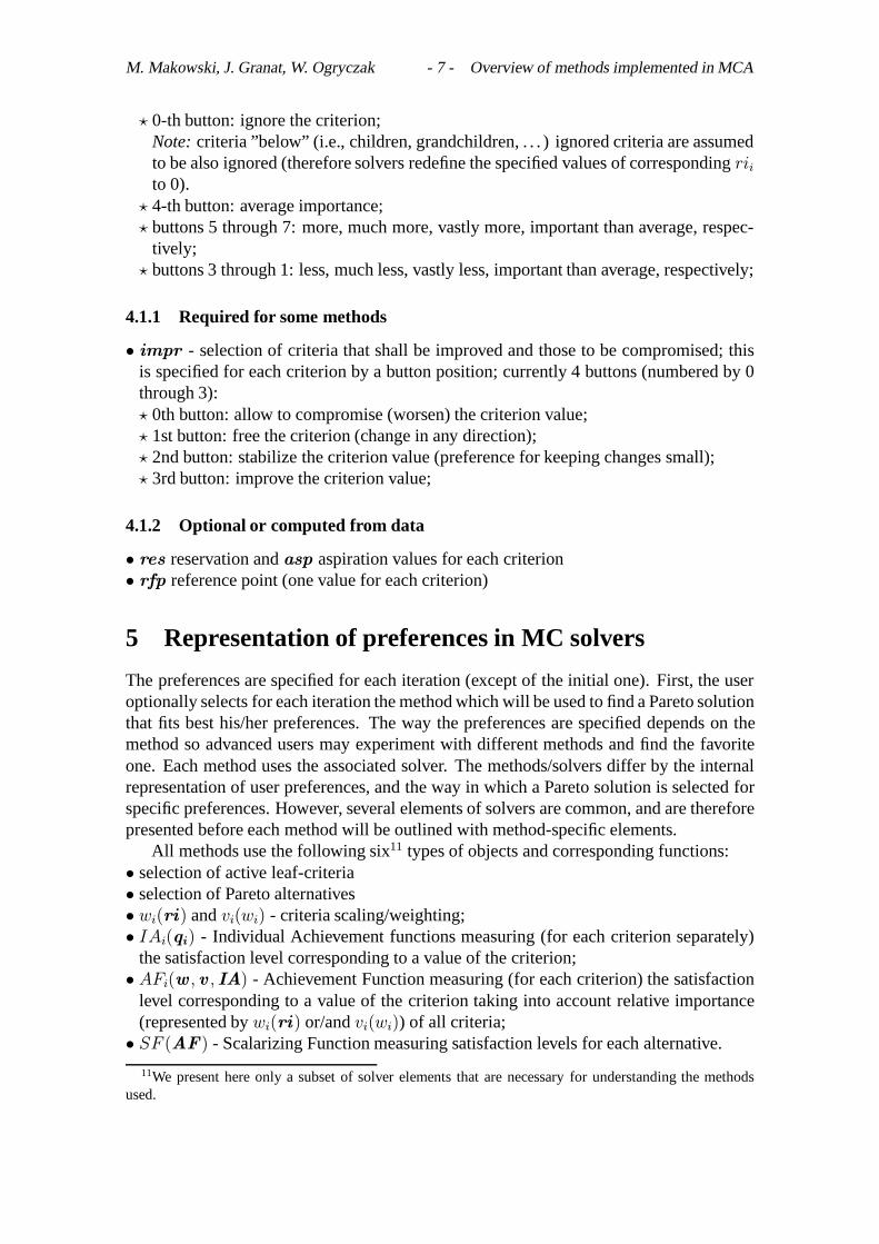
Figure 2: Hierarchy of active criteria

The user may chose to ignore some criteria (cf Sec. 4.1) therefore the set of active leaf-criteria has to be defined for each iteration. This is a trivial operation for analysis withouthierarchical structure. If criteria hierarchy is defined (see example in Fig. 1) then criteriaat any hierarchy level can be specified as inactive, see example in Fig. 2. In such casesthen the set of active-leaf criteria is defined as follows:• full criteria tree is defined (see Fig. 1).• Activity of all criteria is defined according the selection of the value of relative criteria

importance button (Sec. 4.1).• active criteria tree is defined by removing from the full criteria tree nodes corresponding

to inactive criteria and the branches originating from such nodes.12 Note that activityof criteria imply changes in the impact of the selected relative criteria importance, seeSec. 6.3.12In the example shown in Fig. 2 only two criteria (marked by white nodes) were selected to be not

active. However seven more criteria (marked by gray nodes) become inactive because their parent criteriaare inactive.


• The set of active leaf-criteria is composed of leaves of the active criteria tree.Note: Further on we use the termcriteria for the active leaf-criteria, since only such

criteria are considered for analysis. Also the number of criterian denotes the number ofactive leaf-criteria. The role of intermediate-level active criteria is defined in Sec. 6.3.

6.2 Set of Pareto alternatives

The set of Pareto alternatives13 is defined for the considered criteria according to the com-monly used definition:A solution is called Pareto-efficient, if there is no other solutionfor which at least one criterion has a better value while values of remaining criteria arethe same or better.In other words, one cannot improve any criterion without worseningat least one other criterion. Solutions that are not Pareto efficient are called dominated.

Note that each analysis iteration is actually composed of a series of subproblems de-fined for determining ranking of alternatives (see Sec. 10). For each subproblem a newset of Pareto alternatives is defined.

6.3 Criteria relative importance

Preferences for all but one (described in Sec. 8.1.1) methods described in this note arespecified as relative criteria importanceri , see Sec. 4.1. Theri are mapped into twoassociated vectors:• wi, i = 1, . . . , n• vi, i = 1, . . . , n

Definition of criteria scaling coefficients (traditionally called weights)w is rathercomplex and therefore before presenting it we specify the simple definition ofv com-posed of two stages: First, components ofv are defined as:

vi = 1/wi, i = 1, . . . , n. (1)

Second, thev is normalized using the standard procedure:

vi = vi/

n∑i=1

vi, i = 1, . . . , n (2)

The definition ofw is done in two stages:1. Relative criteria importance (for all active criteria) are mapped into real values using

one of the approaches specified in Sec. 6.3.1 and Sec. 6.3.2, respectively. The choiceof the mapping is specific for the method.

2. Procedure described in Sec. 6.3.3 is applied, if criteria hierarchy is defined.

6.3.1 Standard mapping

For the current implementation (seven importance levels for not ignored criteria) the stan-dard mapping is defined by:

wi = rii/6, i = 1, . . . , ncrit (3)

13Also called: Pareto-efficient solutions, Pareto frontier, non-dominated solutions. For the sake of brevitywe don’t deal here with more advanced concepts, e.g., properly efficient solutions.


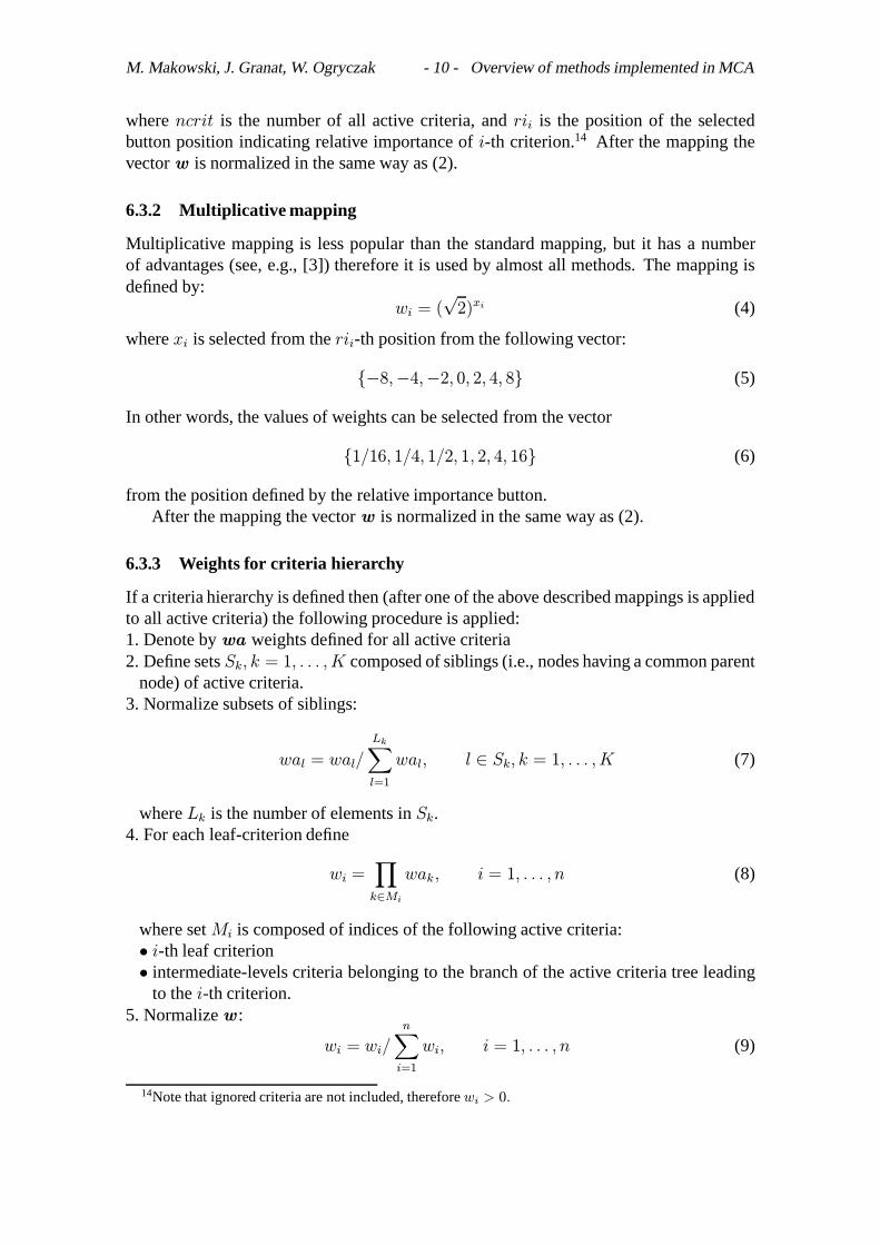
wherencrit is the number of all active criteria, andrii is the position of the selectedbutton position indicating relative importance ofi-th criterion.14 After the mapping thevectorw is normalized in the same way as (2).

6.3.2 Multiplicative mapping

Multiplicative mapping is less popular than the standard mapping, but it has a numberof advantages (see, e.g., [3]) therefore it is used by almost all methods. The mapping isdefined by:

wi = (√

2)xi (4)

wherexi is selected from therii-th position from the following vector:

{−8,−4,−2, 0, 2, 4, 8} (5)

In other words, the values of weights can be selected from the vector

{1/16, 1/4, 1/2, 1, 2, 4, 16} (6)

from the position defined by the relative importance button.After the mapping the vectorw is normalized in the same way as (2).

6.3.3 Weights for criteria hierarchy

If a criteria hierarchy is defined then (after one of the above described mappings is appliedto all active criteria) the following procedure is applied:1. Denote bywa weights defined for all active criteria2. Define setsSk, k = 1, . . . , K composed of siblings (i.e., nodes having a common parent

node) of active criteria.3. Normalize subsets of siblings:

wal = wal/

Lk∑l=1

wal, l ∈ Sk, k = 1, . . . , K (7)

whereLk is the number of elements inSk.4. For each leaf-criterion define

wi =∏k∈Mi

wak, i = 1, . . . , n (8)

where setMi is composed of indices of the following active criteria:• i-th leaf criterion• intermediate-levels criteria belonging to the branch of the active criteria tree leading

to thei-th criterion.5. Normalizew :

wi = wi/

n∑i=1

wi, i = 1, . . . , n (9)

14Note that ignored criteria are not included, thereforewi > 0.


6.4 Individual Achievement Functions

For each criterion define the defaultIAi(qi) (Individual Achievement) function is definedfor each criterion separately.IAi(qi) measures the level of satisfaction (goodness) foreach possible value of the corresponding criterion.

IA functions have the same properties as the Achievement Function in the RFP (Ref-erence Point) method15, in particular to be strictly monotone (increasing/decreasing formaximized/minimized criteria.16). However, in the RFP methods the Achievement Func-tion represents also the inter-criteria preferences. Therefore in the current implementationwe distinguish theIA and theAF functions, both having the same mathematical prop-erties, but the latter including inter-criteria preferences.

IA are defined as follows:1. Denote (for each criterion) by utopia and nadir the best and the worst (over all alterna-

tives) values of the criterion.2. Set the default values ofaspi (aspiration) andresi (reservation) to be equal to the

corresponding utopia and nadir values.3. Implicitly define the defaultIAi(qi) function17 to be a PWL (Piece-Wise Linear) func-

tion composed of one segment:• IAi(nadiri) = IAi(resi) = 0• IAi(utopiai) = IAi(aspi) = 1• IAi(·) ∈ [0, 1]:Note: Such anIA(·) are equivalent to the normalized and unified (to make allmaxi-mized) criteria value mappingsyji in the standard implementations of the weighted-summethods, which typically defineyji as:• scaled and shifted to the rangeyji ∈ [0, 1], j ∈ J, i ∈ I•maximized; i.e. a minimizedy is replaced byy = 1− y.Therefore the default values of utopia, aspiration, reservation, nadir in the weighted-summethod are defined implicitly as:• utopiai = aspi = 1• nadiri = resi = 0

7 Auxiliary functions

The following functions are used by more than one method, therefore we defined themhere.

7.1 Ordered Achievement Functions (OAF)

Ordered achievement function valuesOAF j(·) are defined for each alternative as sorted(in order corresponding to improving the argument values18) of AFi(qj), whereqj is the

15Actually also implicitly used by the WS (Weighted-Sum) method.16Target-type criteria are handled byIA(·) composed of twoIA(·): maximized/minimized for criteria

values smaller/larger than the specified target value.17By qi we denote vector composed ofi-th criterion values (for all alternatives).18Equal values are ordered randomly.


vector of criteria values forj-th alternative):

OAF j = sort(AFi(qj )), j ∈ J (10)

whereAFi(·) is the achievement function specific for each method.

7.2 PWL functions for Quantile Aggregation

Define a PWL (Piece-Wise-Linear) function generated by vector ofn+ 1 points{x ,y}:

xi = i/n, yi, i = 0, 1, . . . , n (11)

whereyy0 = 0; yi = yi−1 + αsi i = 1, . . . , n (12)

wheres denotes preferential OWA weights defined by:

si = 1−(i− 1

n

)0.25

, i = 1, . . . , n (13)

and

α = 1/n∑i=1

si (14)

7.3 Aggregated Ordered Achievement Functions (AOAF)

The concept of Lorenz curves outlined in Appendix A has been adapted for definingAggregated Ordered Achievement FunctionsAOAF .

Two types of aggregation are used which results in twoAOAFs denoted byL1 andL2 , respectively. The first one represents the so-called worst conditional mean which isnatural generalization of the minimum (worst) achievement aggregation. It is defined asthe mean within the specified tolerance level (amount) of the worst achievements. Forthe simplest case one may simply define the worst conditional mean as the mean of thek worst-off achievements (or ratherk/n portion of the worst achievements). This can bemathematically formalized as

L1jk =1

k

k∑l=1

OAFjl (15)

aggregating values ofk-worstOAFj(·)). Note that fork = 1, L1j1 represents the mini-mum achievement, and fork = n,

L1jn =1

n

n∑l=1

OAFjl =1

n

n∑i=1

AFji (16)

which is the mean achievement.


AggregationL1jk can be viewed as a simple transformation of the Absolute LorenzCurve19 for alternativej (denoted byALCj), which is defined as the PWL curve connect-ing the point (0,0) and points:

(i

n,

1

n

i∑l=1

OAFjl) for i = 1, . . . , n. (17)

Exactly,

L1jk =n

kALCj

(k

n

). (18)

Formula (18) is easily extendable for any (not necessarily representing an integer number)fraction of all criteria. Let this fraction be denoted byκ. Then

L1j(κ) =1

κALCj(κ) =

1

nκ

[k∑l=1

OAFjl + (nκ− k)OAFj,k+1

](19)

wherek = bnκc and the corresponding sum is equal to 0 fork = 0.The second aggregation is built as the weighted sum of sorted achievements

L2jk =k−1∑l=1

L2jl + sk ∗OAFjk (20)

with weights

sk =

1 if k = 1 orL2j,k−1 = 0.1

n ∗√k

otherwise (21)

The aggregation is similar the so-called Ordered Weighted Average (OWA) where de-creasing weightssi defined by formula (21) allow us to model decreasing importance ofsubsequenti/n quantiles, i.e., decreasing importance of the second worst criteria values incomparison to the importance of the worst ones, decreasing importance of the third worstcriteria values in comparison to the importance of the second worst ones, etc. Althoughthe weights defined by (21) are alternative dependent which guarantees that all the worstachievements are equally weighted but also differentiate the aggregation from the stan-dard OWA. The relations specified above provide us with faster decreasing of importancefor earlier quantiles and slower for the further ones.

8 Methods

We define here the methods currently implemented in the MCA. Each of them is definedby two functions:• Achievement FunctionsAF that measures (for each criterion) the satisfaction level

corresponding to a value of the criterion taking into account the relative importance ofthis criterion and its individual achievement.• Scalarizing FunctionsSFj(·) which assigns for each alternative a real value. The alter-

native with the largest value ofSFj is selected as the Pareto solution corresponding bestto the specified preferences.

19See Appendix A.


8.1 Objective Choice (OC)

This is the only method which assumes equitable approach, i.e., all criteria having equalimportance. It is typically used for an initial iteration, which is generated automatically,therefore user preferences are unknown (should the method be used by a user then thespecified preferences are ignored).

In the OC method objective values of aspiration and reservation levels are computedfirst, and then used for the AFs.

8.1.1 Objective ASP/RES

Aspiration and reservation values can be defined from the values of the correspondingcriterion, e.g.:

resi = α ∗ averi (22)

aspi = α ∗ (averi + 1) (23)

where the average value ofi-th criterion is defined by:

averi =

m∑j=1

qij/m (24)

wherem is the number of alternatives, andα is a given parameter (currently equal to 0.5).Note: values ofresi andaspi are defined by the data, and therefore will most likely notcorrespond to the actual (i.e. defined by an alternative) criterion value.

8.1.2 Achievement Functions

The AFs are defined as PWL functions composed of three segments defined by the fol-lowing points:• AFi(nadiri) = 0;• AFi(resi) = 3;• AFi(aspi) = 7;• AFi(utopiai) = 10;

Then the values of theAFi(·) are computed as values of such PWL functions for actualvalues ofIAi.

8.1.3 Scalarizing Functions

The values ofAF are used as arguments ofOAF , see eq. (10). ThenSFj are definedby:

SFj = L1j(κ), j ∈ J (25)

whereL1j(κ) is defined by (19), andκ is the criteria quantile that can be changed aftermore experiments. Currently:

κ = float(n)/3, (26)

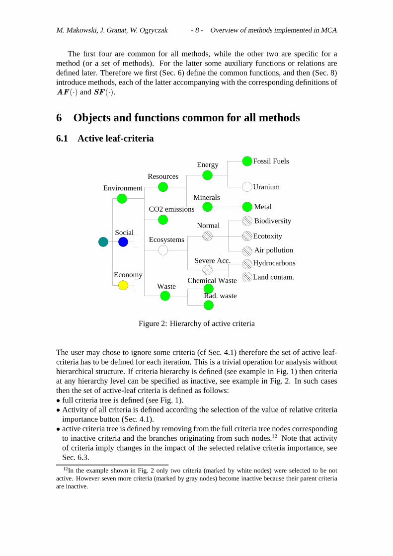
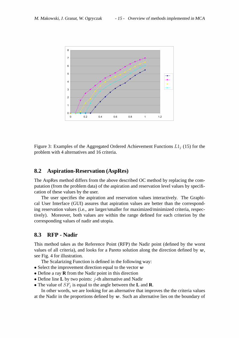
which implies that the selection is based on theAOAF (cumulativeOAFs) defined forthe worst 1/3 of criteria. Illustration of theAOAF is shown in Fig. 3.


0

1

2

3

4

5

6

7

8

0 0.2 0.4 0.6 0.8 1 1.2

��

Figure 3: Examples of the Aggregated Ordered Achievement FunctionsL1j (15) for theproblem with 4 alternatives and 16 criteria.

8.2 Aspiration-Reservation (AspRes)

The AspRes method differs from the above described OC method by replacing the com-putation (from the problem data) of the aspiration and reservation level values by specifi-cation of these values by the user.

The user specifies the aspiration and reservation values interactively. The Graphi-cal User Interface (GUI) assures that aspiration values are better than the correspond-ing reservation values (i.e., are larger/smaller for maximized/minimized criteria, respec-tively). Moreover, both values are within the range defined for each criterion by thecorresponding values of nadir and utopia.

8.3 RFP - Nadir

This method takes as the Reference Point (RFP) the Nadir point (defined by the worstvalues of all criteria), and looks for a Pareto solution along the direction defined byw ,see Fig. 4 for illustration.

The Scalarizing Function is defined in the following way:• Select the improvement direction equal to the vectorw• Define a rayR from the Nadir point in this direction• Define lineL by two points:j-th alternative and Nadir• The value ofSFj is equal to the angle between theL andR.

In other words, we are looking for an alternative that improves the the criteria valuesat the Nadir in the proportions defined byw . Such an alternative lies on the boundary of


q

q1

2

N

w

Figure 4: Nadir-based RFP method. The improvement direction is defined by the scal-ing/weighting vectorw , see eq. (3) or (9).

the cone marked in the Fig. 4 by the gray area. This approach is similar to the WeightedSum (WS – linear criteria aggregation) approach outlined in Sec. 6.3 in the sense thatcriteria improvement ratios are specified as weights. However, the RFP approach avoidsmany deficiencies of the WS method; in particular, it supports analysis of the full Paretoset.

8.4 RFP - Utopia

This method, see Fig. 5 for illustration, is based on a concept similar to that used for theRFP-Nadir method.

q

q

2

1

v

U

Figure 5: Utopia-based RFP method. The direction is defined by the vectorv , see eq. (1).

The Scalarizing Function is defined in the following way:• Select the worsening direction equal to the vectorv• Define a rayR from the Utopia point in this direction• Define lineL by two points:j-th alternative and the Utopia• The value ofSFj is equal to the angle between theL andR.

In other words, we are looking for an alternative that worsens the the criteria values atthe Utopia in the proportions defined byv .


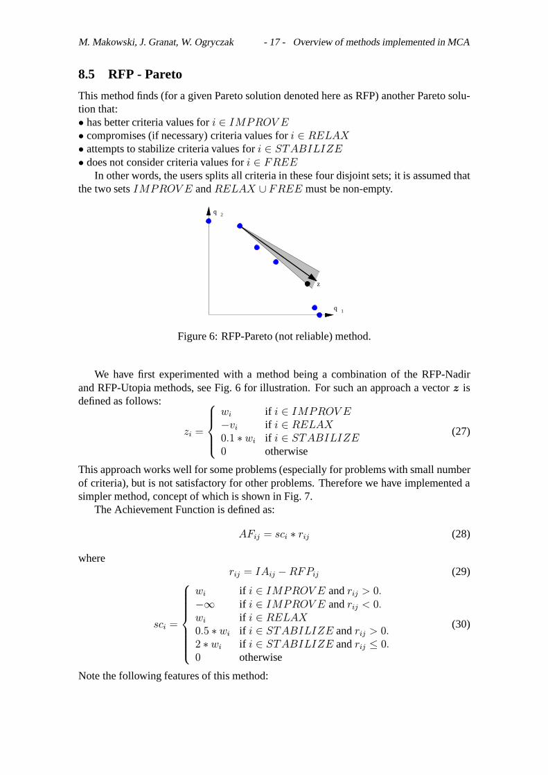
8.5 RFP - Pareto

This method finds (for a given Pareto solution denoted here as RFP) another Pareto solu-tion that:• has better criteria values fori ∈ IMPROV E• compromises (if necessary) criteria values fori ∈ RELAX• attempts to stabilize criteria values fori ∈ STABILIZE• does not consider criteria values fori ∈ FREE

In other words, the users splits all criteria in these four disjoint sets; it is assumed thatthe two setsIMPROV E andRELAX ∪ FREE must be non-empty.

q 2

q 1

z

Figure 6: RFP-Pareto (not reliable) method.

We have first experimented with a method being a combination of the RFP-Nadirand RFP-Utopia methods, see Fig. 6 for illustration. For such an approach a vectorz isdefined as follows:

zi =

wi if i ∈ IMPROV E−vi if i ∈ RELAX0.1 ∗ wi if i ∈ STABILIZE0 otherwise

(27)

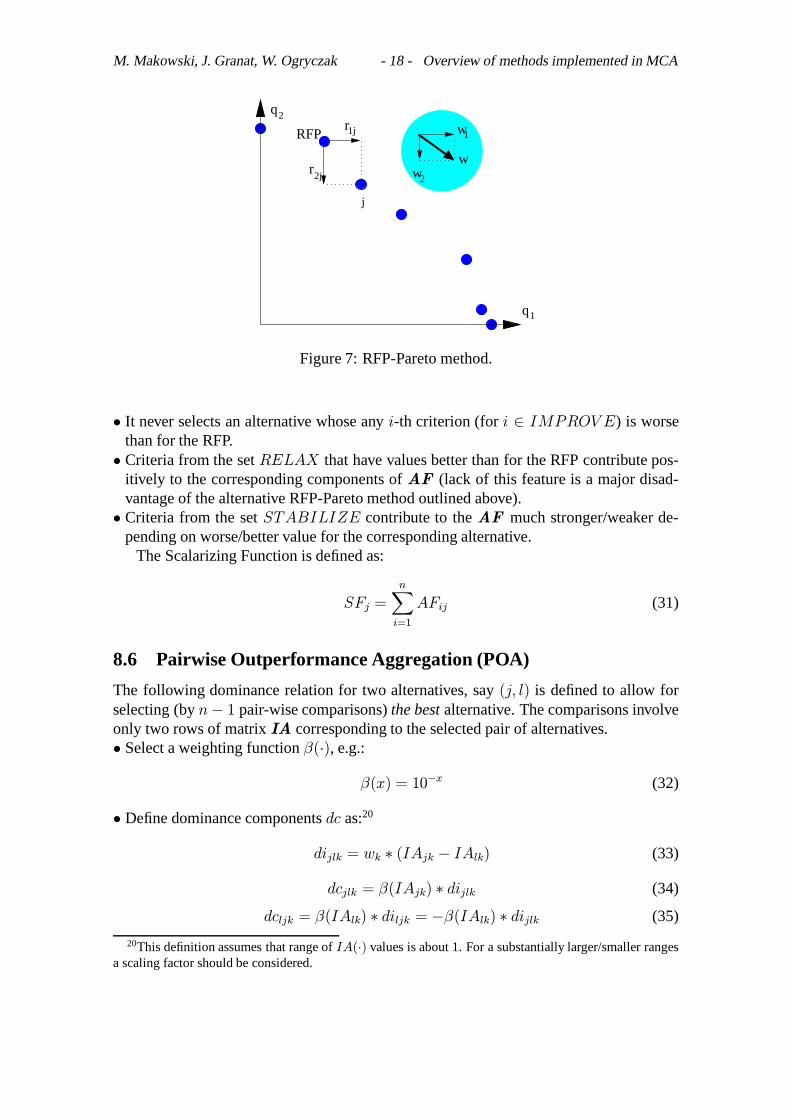
This approach works well for some problems (especially for problems with small numberof criteria), but is not satisfactory for other problems. Therefore we have implemented asimpler method, concept of which is shown in Fig. 7.

The Achievement Function is defined as:

AFij = sci ∗ rij (28)

whererij = IAij −RFPij (29)

sci =

wi if i ∈ IMPROV E andrij > 0.−∞ if i ∈ IMPROV E andrij < 0.wi if i ∈ RELAX0.5 ∗ wi if i ∈ STABILIZE andrij > 0.2 ∗ wi if i ∈ STABILIZE andrij ≤ 0.0 otherwise

(30)

Note the following features of this method:


2j

j

q

q

2

1

RFP

w

r w

wr

1j 1

2

Figure 7: RFP-Pareto method.

• It never selects an alternative whose anyi-th criterion (fori ∈ IMPROV E) is worsethan for the RFP.• Criteria from the setRELAX that have values better than for the RFP contribute pos-

itively to the corresponding components ofAF (lack of this feature is a major disad-vantage of the alternative RFP-Pareto method outlined above).• Criteria from the setSTABILIZE contribute to theAF much stronger/weaker de-

pending on worse/better value for the corresponding alternative.The Scalarizing Function is defined as:

SFj =n∑i=1

AFij (31)

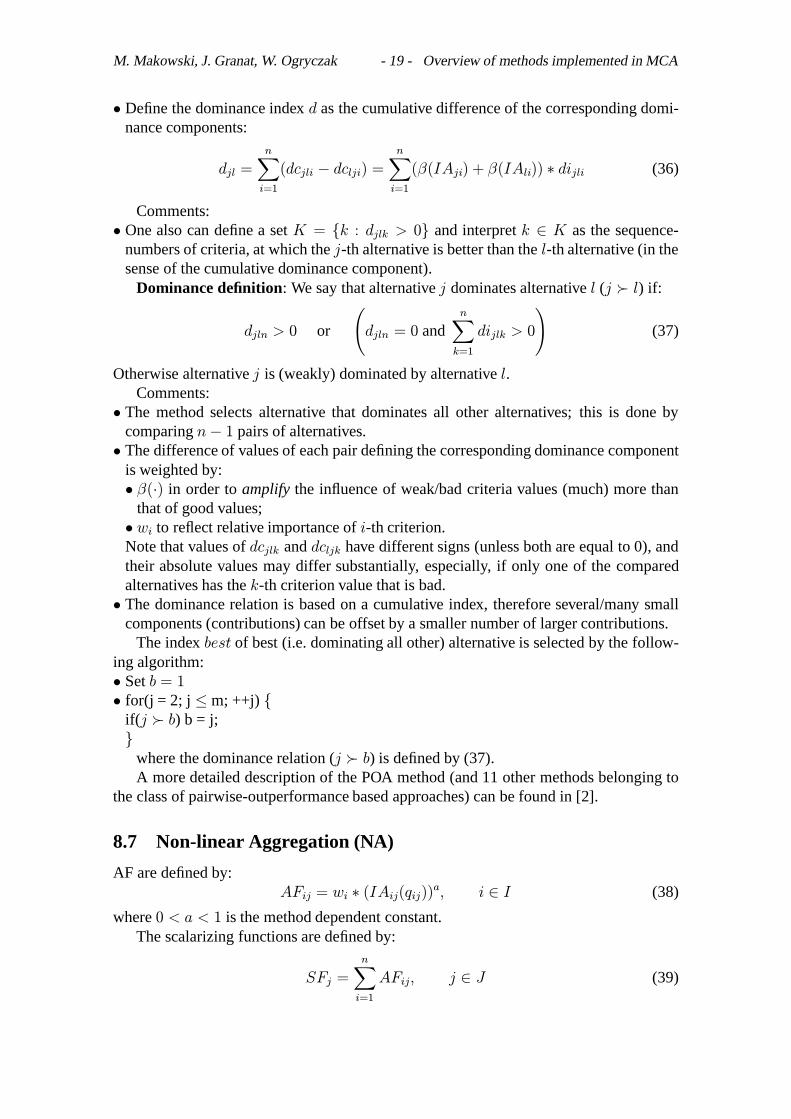
8.6 Pairwise Outperformance Aggregation (POA)

The following dominance relation for two alternatives, say(j, l) is defined to allow forselecting (byn− 1 pair-wise comparisons)the bestalternative. The comparisons involveonly two rows of matrixIA corresponding to the selected pair of alternatives.• Select a weighting functionβ(·), e.g.:

β(x) = 10−x (32)

• Define dominance componentsdc as:20

dijlk = wk ∗ (IAjk − IAlk) (33)

dcjlk = β(IAjk) ∗ dijlk (34)

dcljk = β(IAlk) ∗ diljk = −β(IAlk) ∗ dijlk (35)

20This definition assumes that range ofIA(·) values is about 1. For a substantially larger/smaller rangesa scaling factor should be considered.


• Define the dominance indexd as the cumulative difference of the corresponding domi-nance components:

djl =n∑i=1

(dcjli − dclji) =n∑i=1

(β(IAji) + β(IAli)) ∗ dijli (36)

Comments:• One also can define a setK = {k : djlk > 0} and interpretk ∈ K as the sequence-

numbers of criteria, at which thej-th alternative is better than thel-th alternative (in thesense of the cumulative dominance component).

Dominance definition: We say that alternativej dominates alternativel (j � l) if:

djln > 0 or

(djln = 0 and

n∑k=1

dijlk > 0

)(37)

Otherwise alternativej is (weakly) dominated by alternativel.Comments:

• The method selects alternative that dominates all other alternatives; this is done bycomparingn− 1 pairs of alternatives.• The difference of values of each pair defining the corresponding dominance component

is weighted by:• β(·) in order toamplify the influence of weak/bad criteria values (much) more than

that of good values;• wi to reflect relative importance ofi-th criterion.Note that values ofdcjlk anddcljk have different signs (unless both are equal to 0), andtheir absolute values may differ substantially, especially, if only one of the comparedalternatives has thek-th criterion value that is bad.• The dominance relation is based on a cumulative index, therefore several/many small

components (contributions) can be offset by a smaller number of larger contributions.The indexbest of best (i.e. dominating all other) alternative is selected by the follow-

ing algorithm:• Setb = 1• for(j = 2; j ≤m; ++j) {

if(j � b) b = j;}

where the dominance relation (j � b) is defined by (37).A more detailed description of the POA method (and 11 other methods belonging to

the class of pairwise-outperformance based approaches) can be found in [2].

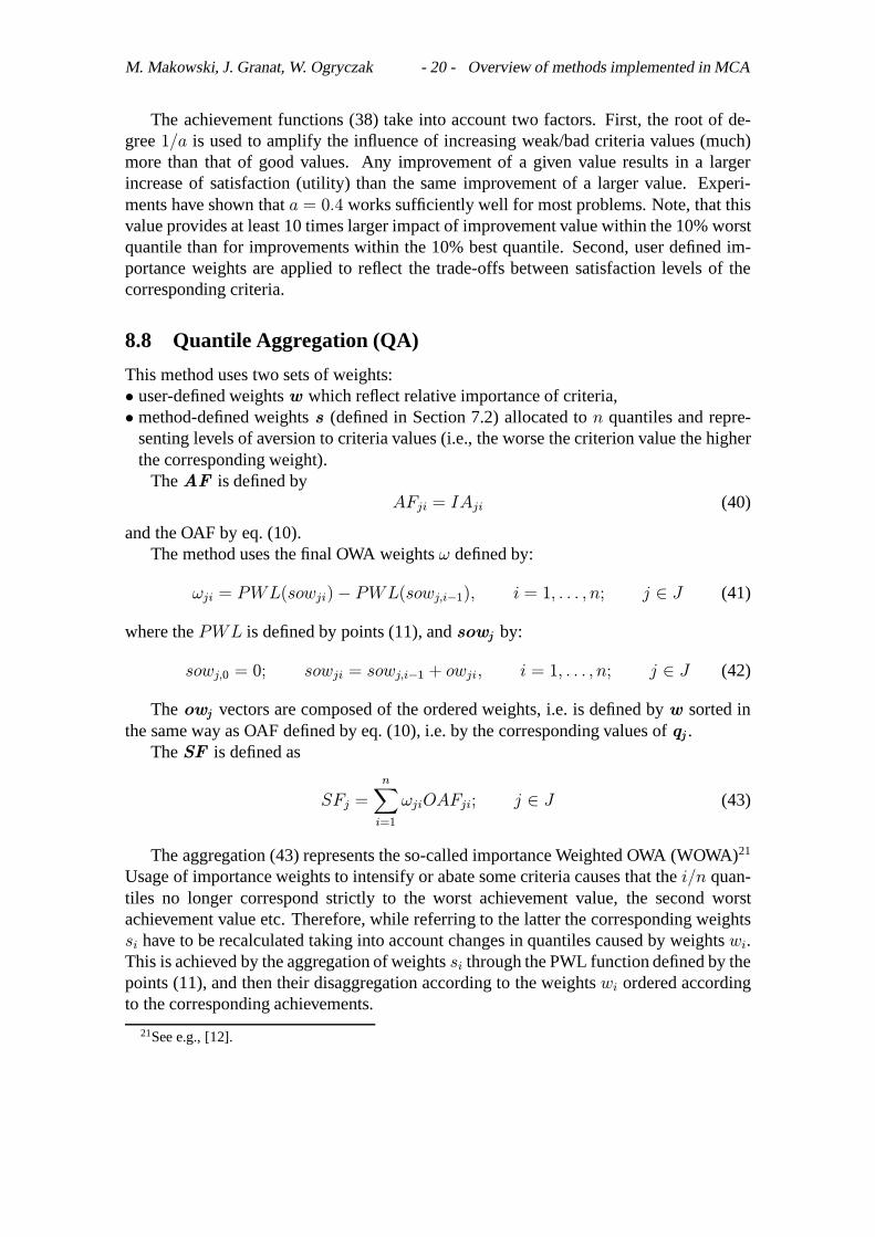
8.7 Non-linear Aggregation (NA)

AF are defined by:AFij = wi ∗ (IAij(qij))

a, i ∈ I (38)

where0 < a < 1 is the method dependent constant.The scalarizing functions are defined by:

SFj =n∑i=1

AFij, j ∈ J (39)


The achievement functions (38) take into account two factors. First, the root of de-gree1/a is used to amplify the influence of increasing weak/bad criteria values (much)more than that of good values. Any improvement of a given value results in a largerincrease of satisfaction (utility) than the same improvement of a larger value. Experi-ments have shown thata = 0.4 works sufficiently well for most problems. Note, that thisvalue provides at least 10 times larger impact of improvement value within the 10% worstquantile than for improvements within the 10% best quantile. Second, user defined im-portance weights are applied to reflect the trade-offs between satisfaction levels of thecorresponding criteria.

8.8 Quantile Aggregation (QA)

This method uses two sets of weights:• user-defined weightsw which reflect relative importance of criteria,• method-defined weightss (defined in Section 7.2) allocated ton quantiles and repre-

senting levels of aversion to criteria values (i.e., the worse the criterion value the higherthe corresponding weight).

TheAF is defined byAFji = IAji (40)

and the OAF by eq. (10).The method uses the final OWA weightsω defined by:

ωji = PWL(sowji)− PWL(sowj,i−1), i = 1, . . . , n; j ∈ J (41)

where thePWL is defined by points (11), andsowj by:

sowj,0 = 0; sowji = sowj,i−1 + owji, i = 1, . . . , n; j ∈ J (42)

Theowj vectors are composed of the ordered weights, i.e. is defined byw sorted inthe same way as OAF defined by eq. (10), i.e. by the corresponding values ofqj .

TheSF is defined as

SFj =n∑i=1

ωjiOAFji; j ∈ J (43)

The aggregation (43) represents the so-called importance Weighted OWA (WOWA)21

Usage of importance weights to intensify or abate some criteria causes that thei/n quan-tiles no longer correspond strictly to the worst achievement value, the second worstachievement value etc. Therefore, while referring to the latter the corresponding weightssi have to be recalculated taking into account changes in quantiles caused by weightswi.This is achieved by the aggregation of weightssi through the PWL function defined by thepoints (11), and then their disaggregation according to the weightswi ordered accordingto the corresponding achievements.

21See e.g., [12].


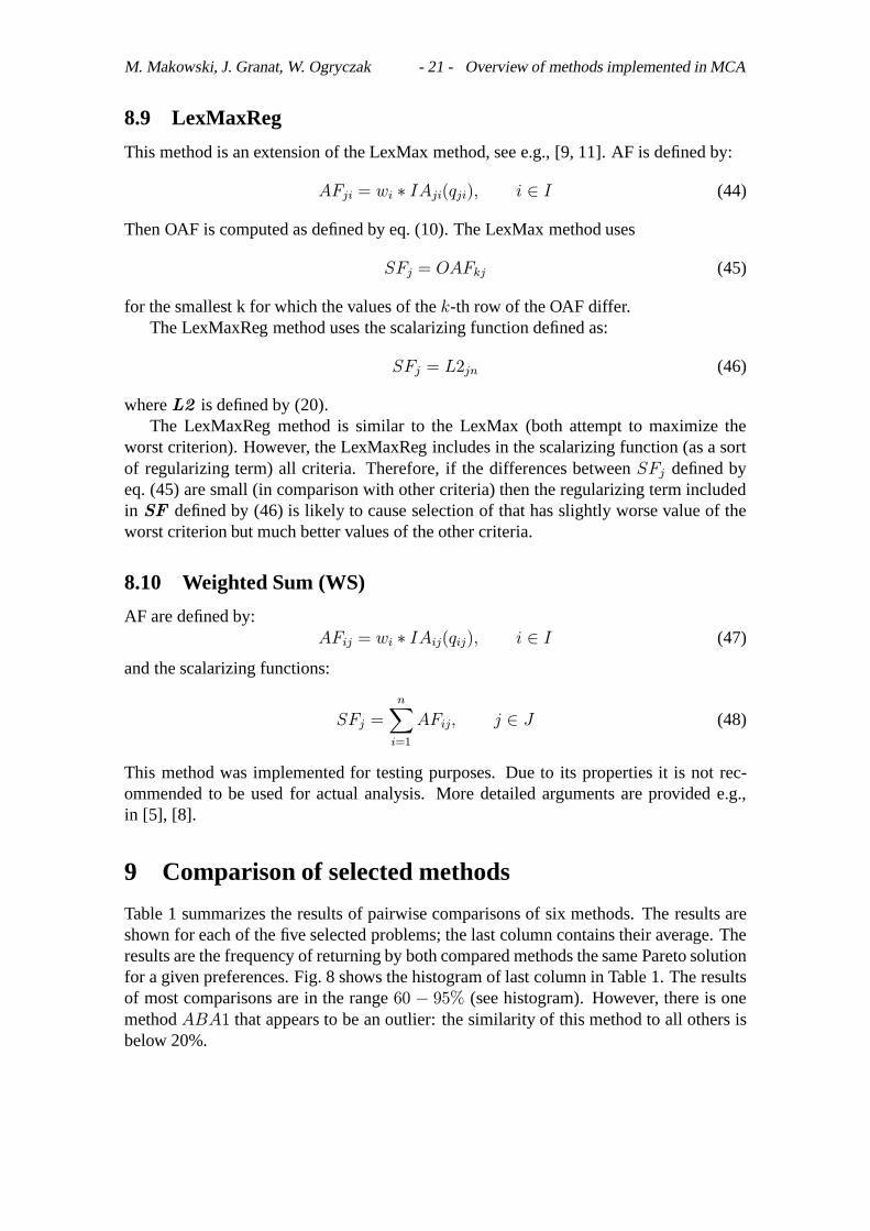
8.9 LexMaxReg

This method is an extension of the LexMax method, see e.g., [9, 11]. AF is defined by:

AFji = wi ∗ IAji(qji), i ∈ I (44)

Then OAF is computed as defined by eq. (10). The LexMax method uses

SFj = OAFkj (45)

for the smallest k for which the values of thek-th row of the OAF differ.The LexMaxReg method uses the scalarizing function defined as:

SFj = L2jn (46)

whereL2 is defined by (20).The LexMaxReg method is similar to the LexMax (both attempt to maximize the

worst criterion). However, the LexMaxReg includes in the scalarizing function (as a sortof regularizing term) all criteria. Therefore, if the differences betweenSFj defined byeq. (45) are small (in comparison with other criteria) then the regularizing term includedin SF defined by (46) is likely to cause selection of that has slightly worse value of theworst criterion but much better values of the other criteria.

8.10 Weighted Sum (WS)

AF are defined by:AFij = wi ∗ IAij(qij), i ∈ I (47)

and the scalarizing functions:

SFj =n∑i=1

AFij, j ∈ J (48)

This method was implemented for testing purposes. Due to its properties it is not rec-ommended to be used for actual analysis. More detailed arguments are provided e.g.,in [5], [8].

9 Comparison of selected methods

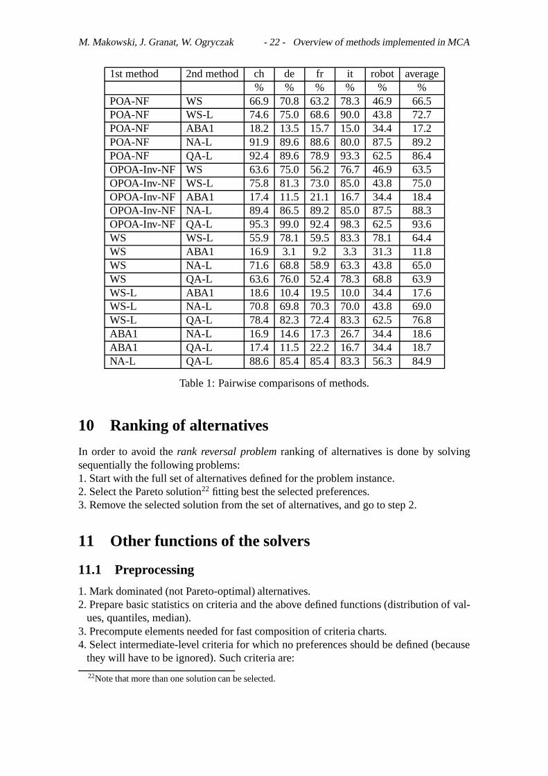
Table 1 summarizes the results of pairwise comparisons of six methods. The results areshown for each of the five selected problems; the last column contains their average. Theresults are the frequency of returning by both compared methods the same Pareto solutionfor a given preferences. Fig. 8 shows the histogram of last column in Table 1. The resultsof most comparisons are in the range60 − 95% (see histogram). However, there is onemethodABA1 that appears to be an outlier: the similarity of this method to all others isbelow 20%.


1st method 2nd method ch de fr it robot average% % % % % %

POA-NF WS 66.9 70.8 63.2 78.3 46.9 66.5POA-NF WS-L 74.6 75.0 68.6 90.0 43.8 72.7POA-NF ABA1 18.2 13.5 15.7 15.0 34.4 17.2POA-NF NA-L 91.9 89.6 88.6 80.0 87.5 89.2POA-NF QA-L 92.4 89.6 78.9 93.3 62.5 86.4OPOA-Inv-NF WS 63.6 75.0 56.2 76.7 46.9 63.5OPOA-Inv-NF WS-L 75.8 81.3 73.0 85.0 43.8 75.0OPOA-Inv-NF ABA1 17.4 11.5 21.1 16.7 34.4 18.4OPOA-Inv-NF NA-L 89.4 86.5 89.2 85.0 87.5 88.3OPOA-Inv-NF QA-L 95.3 99.0 92.4 98.3 62.5 93.6WS WS-L 55.9 78.1 59.5 83.3 78.1 64.4WS ABA1 16.9 3.1 9.2 3.3 31.3 11.8WS NA-L 71.6 68.8 58.9 63.3 43.8 65.0WS QA-L 63.6 76.0 52.4 78.3 68.8 63.9WS-L ABA1 18.6 10.4 19.5 10.0 34.4 17.6WS-L NA-L 70.8 69.8 70.3 70.0 43.8 69.0WS-L QA-L 78.4 82.3 72.4 83.3 62.5 76.8ABA1 NA-L 16.9 14.6 17.3 26.7 34.4 18.6ABA1 QA-L 17.4 11.5 22.2 16.7 34.4 18.7NA-L QA-L 88.6 85.4 85.4 83.3 56.3 84.9

Table 1: Pairwise comparisons of methods.

10 Ranking of alternatives

In order to avoid therank reversal problemranking of alternatives is done by solvingsequentially the following problems:1. Start with the full set of alternatives defined for the problem instance.2. Select the Pareto solution22 fitting best the selected preferences.3. Remove the selected solution from the set of alternatives, and go to step 2.

11 Other functions of the solvers

11.1 Preprocessing

1. Mark dominated (not Pareto-optimal) alternatives.2. Prepare basic statistics on criteria and the above defined functions (distribution of val-

ues, quantiles, median).3. Precompute elements needed for fast composition of criteria charts.4. Select intermediate-level criteria for which no preferences should be defined (because

they will have to be ignored). Such criteria are:

22Note that more than one solution can be selected.


0 10 20 30 40 50 60 70 80 90 1000

1

2

3

4

5

6

Figure 8: Histogram of the average frequency of the comparison results.

• if a higher-level criterion is the only child;• if the leaf-criterion is the only child, then preferences are not specified for its parent.

5. Define the structures needed for possibly fast execution of the GUI (run as a Webclient).

11.2 Info provided with the bestalternative

Generally interaction should be done in the criteria space, i.e., we assume that the userswill consider/analyze trade-offs in terms of criteria values. Thebestalternative (i.e., theone corresponding best to the specified preferences) implies the corresponding trade-offsbetween criteria values.1. For facilitating interaction (aimed at verifying/modifying preferences) we provide pos-

sibly clear information about the criteria ofbestalternative, and help in examining fea-sible changes in the criteria space.

2. The user can display for any selected subset of alternatives the characteristics of:• criteria for which the alternative isstrong• criteria for which the alternative isweak

3. Ranking resulting from the procedure described in Sec. 10 is provided in the graphicalform.

4. Values of theSF are also available as a chart.

11.3 More info about the MCA

Detailed user guide and tutorial to the MCA is available in [6]. It contains also informationabout access to the MCA, which is free for research and educational purposes.


References

[1] GRANAT, J., AND MAKOWSKI, M. Multicriteria methodology for the NEEDSproject. Interim Report IR-09-10, International Institute for Applied Systems Anal-ysis, Laxenburg, Austria, 2009.

[2] GRANAT, J., MAKOWSKI, M., AND OGRYCZAK, W. Multiple criteria anal-ysis of discrete alternatives with a simple preference specification: Pairwise-outperformance approaches. Interim Report IR-09-23, International Institute forApplied Systems Analysis, Laxenburg, Austria, 2009.

[3] L OOTSMA, F. Multi Criteria Decision Analysis via Ratio and Difference Judgement,vol. 29 of Applied Optimization. Kluwer Academic Publishers, Boston, London,1999.

[4] L ORENZ, M. Methods of measuring the concentration of wealth.Publications ofthe American Statistical Association 9(1905), 209–219. doi:10.2307/2276207.

[5] M AKOWSKI, M. Management of attainable tradeoffs between conflicting goals.Journal of Computers 4, 10 (2009), 1033–1042. ISSN 1796-203X.

[6] M AKOWSKI, M., GRANAT, J., AND REN, H. User guide to MCA: Multi-criteriaanalysis of discrete alternatives with a simple preference specification. InterimReport IR-09-22, International Institute for Applied Systems Analysis, Laxenburg,Austria, 2009.

[7] M AKOWSKI, M., GRANAT, J., REN, H., SCHENLER, W., AND HIRSCHBERG,S. Requirement analysis and implementation of the multicriteria analysis in theNEEDS project. Interim Report IR-09-09, International Institute for Applied Sys-tems Analysis, Laxenburg, Austria, 2009.

[8] M AKOWSKI, M., AND WIERZBICKI, A. Modeling knowledge: Model-based de-cision support and soft computations. InApplied Decision Support with Soft Com-puting, X. Yu and J. Kacprzyk, Eds., vol. 124 ofSeries: Studies in Fuzziness andSoft Computing. Springer-Verlag, Berlin, New York, 2003, pp. 3–60. ISBN 3-540-02491-3, draft version available fromhttp://www.iiasa.ac.at/˜marek/pubs/prepub.html .

[9] OGRYCZAK, W. On the lexicographic minimax approach to location problems.European Journal of Operational Research 100(1997), 566–585.

[10] OGRYCZAK, W., AND SLIWINSKI , T. On equitable approaches to resource alloca-tion problems: The conditional minimax solutions.Journal of Telecommunicationsand Information Technology, 3 (2002), 40–48.

[11] OGRYCZAK, W., AND SLIWINSKI , T. On direct methods for lexicographic min-max optimization. InComputational Science and Its Applications-ICCSA 2006,no. 3982 in Lecture Notes in Computer Science. Springer, Berlin, 2006, pp. 802–811.


[12] TORRA, V. The weighted OWA operator.Int. J. Intell. Syst. 12(1997), 153–166.

[13] WIERZBICKI , A., MAKOWSKI, M., AND WESSELS, J., Eds. Model-Based De-cision Support Methodology with Environmental Applications. Series: Mathemat-ical Modeling and Applications. Kluwer Academic Publishers, Dordrecht, 2000.ISBN 0-7923-6327-2.

[14] YAGER, R. On ordered weighted averaging aggregation operators in multicriteriadecision making.IEEE Trans. Systems, Man and Cyber. 18(1988), 183–190.

[15] YAGER, R., AND KACPRZYK, J., Eds.The Ordered Weighted Averaging Operators:Theory and Applications. Kluwer, Dordrecht, 1997.


A Lorenz curve and quantile measures

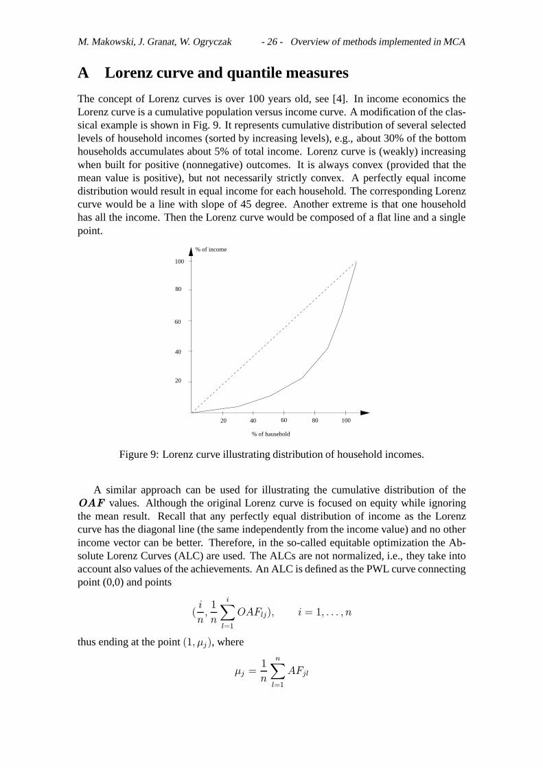
The concept of Lorenz curves is over 100 years old, see [4]. In income economics theLorenz curve is a cumulative population versus income curve. A modification of the clas-sical example is shown in Fig. 9. It represents cumulative distribution of several selectedlevels of household incomes (sorted by increasing levels), e.g., about 30% of the bottomhouseholds accumulates about 5% of total income. Lorenz curve is (weakly) increasingwhen built for positive (nonnegative) outcomes. It is always convex (provided that themean value is positive), but not necessarily strictly convex. A perfectly equal incomedistribution would result in equal income for each household. The corresponding Lorenzcurve would be a line with slope of 45 degree. Another extreme is that one householdhas all the income. Then the Lorenz curve would be composed of a flat line and a singlepoint.

20

% of income

% of hausehold

20 60 1008040

100

80

60

40

Figure 9: Lorenz curve illustrating distribution of household incomes.

A similar approach can be used for illustrating the cumulative distribution of theOAF values. Although the original Lorenz curve is focused on equity while ignoringthe mean result. Recall that any perfectly equal distribution of income as the Lorenzcurve has the diagonal line (the same independently from the income value) and no otherincome vector can be better. Therefore, in the so-called equitable optimization the Ab-solute Lorenz Curves (ALC) are used. The ALCs are not normalized, i.e., they take intoaccount also values of the achievements. An ALC is defined as the PWL curve connectingpoint (0,0) and points

(i

n,

1

n

i∑l=1

OAFlj), i = 1, . . . , n

thus ending at the point(1, µj), where

µj =1

n

n∑l=1

AFjl


6

-

ALC

in

1

r

r

��,

,

,

,

,,

p

p

p

p

p

p

p

p

p

p

p

p

p

p

p

p

p

p

p

p

p

p

p

p

p

p

p

p

p

p

p

p

p

p

p

p

p

p

p

p

r

r

((((

((��,

,

,

,

,,

��

23

13

0

0.3

0.6

q 1

q 2

q 3

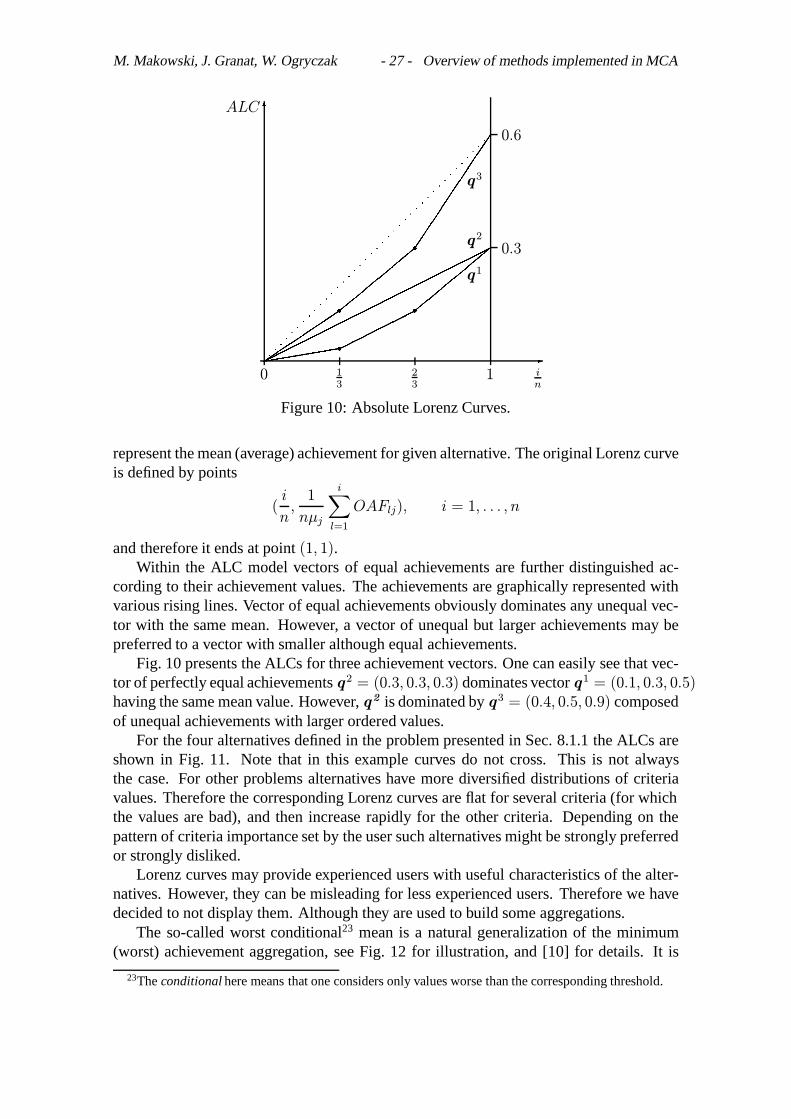
Figure 10: Absolute Lorenz Curves.

represent the mean (average) achievement for given alternative. The original Lorenz curveis defined by points

(i

n,

1

nµj

i∑l=1

OAFlj), i = 1, . . . , n

and therefore it ends at point(1, 1).Within the ALC model vectors of equal achievements are further distinguished ac-

cording to their achievement values. The achievements are graphically represented withvarious rising lines. Vector of equal achievements obviously dominates any unequal vec-tor with the same mean. However, a vector of unequal but larger achievements may bepreferred to a vector with smaller although equal achievements.

Fig. 10 presents the ALCs for three achievement vectors. One can easily see that vec-tor of perfectly equal achievementsq 2 = (0.3, 0.3, 0.3) dominates vectorq 1 = (0.1, 0.3, 0.5)having the same mean value. However,q2 is dominated byq 3 = (0.4, 0.5, 0.9) composedof unequal achievements with larger ordered values.

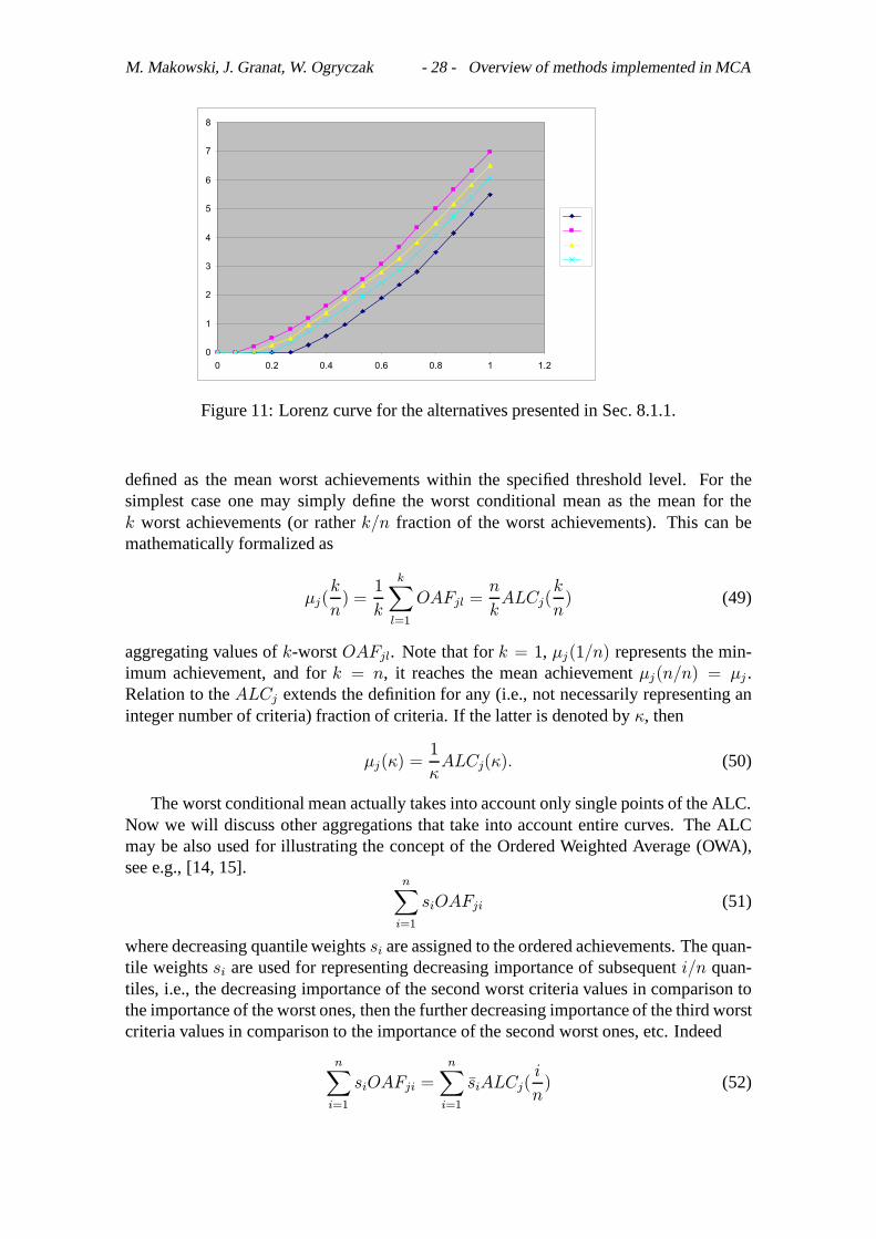
For the four alternatives defined in the problem presented in Sec. 8.1.1 the ALCs areshown in Fig. 11. Note that in this example curves do not cross. This is not alwaysthe case. For other problems alternatives have more diversified distributions of criteriavalues. Therefore the corresponding Lorenz curves are flat for several criteria (for whichthe values are bad), and then increase rapidly for the other criteria. Depending on thepattern of criteria importance set by the user such alternatives might be strongly preferredor strongly disliked.

Lorenz curves may provide experienced users with useful characteristics of the alter-natives. However, they can be misleading for less experienced users. Therefore we havedecided to not display them. Although they are used to build some aggregations.

The so-called worst conditional23 mean is a natural generalization of the minimum(worst) achievement aggregation, see Fig. 12 for illustration, and [10] for details. It is

23Theconditionalhere means that one considers only values worse than the corresponding threshold.


0

1

2

3

4

5

6

7

8

0 0.2 0.4 0.6 0.8 1 1.2

��

Figure 11: Lorenz curve for the alternatives presented in Sec. 8.1.1.

defined as the mean worst achievements within the specified threshold level. For thesimplest case one may simply define the worst conditional mean as the mean for thek worst achievements (or ratherk/n fraction of the worst achievements). This can bemathematically formalized as

µj(k

n) =

1

k

k∑l=1

OAFjl =n

kALCj(

k

n) (49)

aggregating values ofk-worstOAFjl. Note that fork = 1, µj(1/n) represents the min-imum achievement, and fork = n, it reaches the mean achievementµj(n/n) = µj .Relation to theALCj extends the definition for any (i.e., not necessarily representing aninteger number of criteria) fraction of criteria. If the latter is denoted byκ, then

µj(κ) =1

κALCj(κ). (50)

The worst conditional mean actually takes into account only single points of the ALC.Now we will discuss other aggregations that take into account entire curves. The ALCmay be also used for illustrating the concept of the Ordered Weighted Average (OWA),see e.g., [14, 15].

n∑i=1

siOAFji (51)

where decreasing quantile weightssi are assigned to the ordered achievements. The quan-tile weightssi are used for representing decreasing importance of subsequenti/n quan-tiles, i.e., the decreasing importance of the second worst criteria values in comparison tothe importance of the worst ones, then the further decreasing importance of the third worstcriteria values in comparison to the importance of the second worst ones, etc. Indeed

n∑i=1

siOAFji =n∑i=1

siALCj(i

n) (52)


6

-��

1

ALCj

in

��

��

��

��

miniAFji

µj(κ)

µj

κ1n

2n

0

Figure 12: Absolute Lorenz Curve and the worst conditional mean.

with weightssi = si − si+1, i = 1, . . . , n− 1; sn = sn. (53)

Hence, the OWA aggregation with the decreasing quantile weights may be viewed as theweighted arithmetic mean of the ALC segments with appropriate positive weights.

For the curves corresponding to the four alternatives illustrated in Fig. 11 the alterna-tive B is dominating all other alternatives in the sense that it has the most equal distributionof criteria values as well as the largest worst conditional means. For equitable preferences(all criteria has the same importance) the alternative B might be also preferred by theuser. However, this reasoning will not be justified if the importance the user attaches tocriteria differ. A justification for selecting another alternative might be that the criteriawith higher importance have better values (note that the OAFs are sorted, and typicallydifferent criteria are the worst ones for different alternatives).

The OWA aggregation (51) is built for equally important achievements where only thedistribution of achievements values is evaluated. Actually, achievement vectors havingthe same OWA value may differ only by the order of achievement values. For instance,consider two symmetric achievements vectorsq 1 = (0, 1) andq 2 = (1, 0), and OWAweightss1 = 0.9 ands2 = 0.1; the OWA aggregation for both vectors is equal:

OWA1 = OWA2 = 0.9 · 0 + 0.1 · 1 = 0.1.

However, the users typically want to associate different importance to the elements ofachievement vectors. This can be done by introducing into the OWA aggregation theimportance weightswi, which define a repetition measure within the distribution (popu-lation) of achievement values. Note, that the OWA weightssi are applied to the averageswithin specific quantiles of size1/n for this distribution. To illustrate this concept letus consider the importance weightsw1 = 0.75 andw2 = 0.25. Then the achievementvectorq 1 = (0, 1) is represented by the distribution having the value 0 with the repe-tition measure 0.75, and the value 1 with the repetition measure 0.25; the achievementvectorq 2 = (1, 0) is represented by the distribution having the value 1 with the repetition


measure 0.75, and the value 0 with the repetition measure 0.25. In this specific case, thedistributions may be equivalently interpreted in four dimensional space of equally impor-tant achievements (applying the measure of 0.25 to each element) where the original firstachievement has been triplicated; thusq 1 = (0, 0, 0, 1) andq 2 = (1, 1, 1, 0). The OWAaggregation with weightss1 = 0.9 ands2 = 0.1 applied to the corresponding averageswithin quantiles of size0.5 results in the aggregation values0.9 ·0+0.1 ·(0+1)/2 = 0.05for q 1, and0.9 · (0 + 1)/2 + 0.1 · 1 = 0.55 for q 2, respectively.

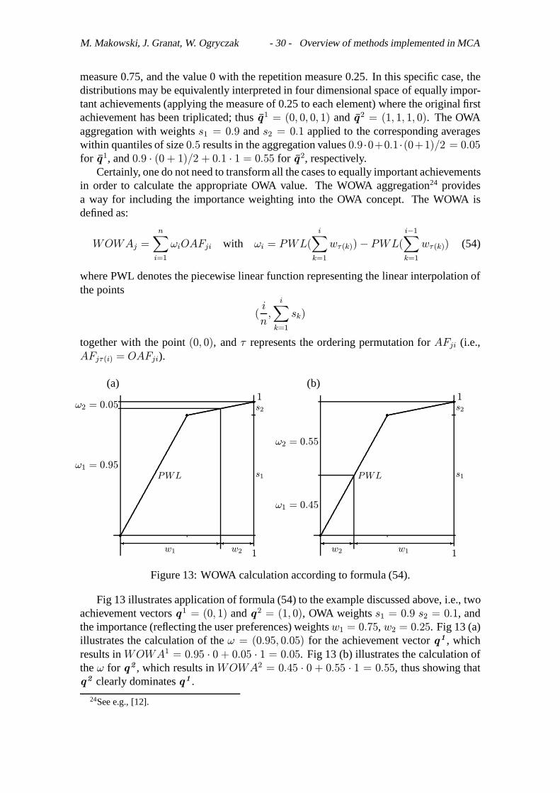
Certainly, one do not need to transform all the cases to equally important achievementsin order to calculate the appropriate OWA value. The WOWA aggregation24 providesa way for including the importance weighting into the OWA concept. The WOWA isdefined as:

WOWAj =

n∑i=1

ωiOAFji with ωi = PWL(

i∑k=1

wτ (k))− PWL(

i−1∑k=1

wτ (k)) (54)

where PWL denotes the piecewise linear function representing the linear interpolation ofthe points

(i

n,

i∑k=1

sk)

together with the point(0, 0), andτ represents the ordering permutation forAFji (i.e.,AFjτ (i) = OAFji).

r

r

r

1

1

s1

s2

PWLω1 = 0.95

ω2 = 0.05

-� -�w1 w2

(a)

r

r

r

1

1

s1

s2

PWL

ω1 = 0.45

ω2 = 0.55

-� -�w2 w1

(b)

Figure 13: WOWA calculation according to formula (54).

Fig 13 illustrates application of formula (54) to the example discussed above, i.e., twoachievement vectorsq 1 = (0, 1) andq 2 = (1, 0), OWA weightss1 = 0.9 s2 = 0.1, andthe importance (reflecting the user preferences) weightsw1 = 0.75, w2 = 0.25. Fig 13 (a)illustrates the calculation of theω = (0.95, 0.05) for the achievement vectorq1 , whichresults inWOWA1 = 0.95 · 0 + 0.05 · 1 = 0.05. Fig 13 (b) illustrates the calculation oftheω for q2 , which results inWOWA2 = 0.45 · 0 + 0.55 · 1 = 0.55, thus showing thatq2 clearly dominatesq1 .

24See e.g., [12].

interim report ir-09-24 overview of methods implemented in

Documents