intermittentsearchstrategies - École polytechnique 83, 81-… · distribution of targets 107 3....

Intermittent search strategies

O. Benichou, C. Loverdo, M. Moreau, and R. Voituriez

UPMC Universite de Paris 06, UMR 7600 Laboratoire de Physique Theorique de la MatiereCondensee, 4 Place Jussieu, F-75005 Paris, France

(Received 25 January 2010; published 28 March 2011)

This review examines intermittent target search strategies, which combine phases of slow motion,

allowing the searcher to detect the target, and phases of fast motion during which targets cannot be

detected. It is first shown that intermittent search strategies are actually widely observed at various

scales. At the macroscopic scale, this is, for example, the case of animals looking for food; at the

microscopic scale, intermittent transport patterns are involved in a reaction pathway of DNA-

binding proteins as well as in intracellular transport. Second, generic stochastic models are

introduced, which show that intermittent strategies are efficient strategies that enable the minimi-

zation of search time. This suggests that the intrinsic efficiency of intermittent search strategies

could justify their frequent observation in nature. Last, beyond these modeling aspects, it is

proposed that intermittent strategies could also be used in a broader context to design and accelerate

search processes.

DOI: 10.1103/RevModPhys.83.81 PACS numbers: 05.40.�a, 87.10.�e

CONTENTS

I. Introduction 82

A. General scope and outline 82

B. General framework and first definitions 83

1. Searching with or without cues 83

2. Systematic versus random strategies 83

3. Framework 84

II. Intermittent Search Strategies at the Macroscopic Scale 84

A. The Levy strategies 84

1. The advantage of Levy walks with respect

to simple random walks 84

2. Optimizing the encounter rate with Levy

walks: How and when? 84

B. A basic model of intermittence 86

1. Observations: The case of saltatory animals 86

2. Model 86

3. Equations 86

4. Results 87

5. Comparison with experimental data 87

C. Two-dimensional intermittent search processes:

An alternative to Levy strategies 88

1. Motivation 88

2. Model 88

3. Basic equations 88

4. Results for the diffusive mode of detection 89

5. Results for the static mode of detection 89

6. Conclusion 89

D. Should foraging animals really adopt Levy strategies? 89

1. The albatross story 89

2. Do animals really perform Levy walks? 89

E. Conclusion on animal foraging 90

III. Intermittent Search Strategies at the Microscopic Scale 90

A. Protein-DNA interactions 90

1. Biological context 90

2. Minimal model of intermittent reaction paths 91

3. Toward a more realistic modeling 94

4. Conclusion on protein-DNA interactions 98

B. Active transport of vesicles in cells 98

1. Active transport in cells 99

2. Model 99

3. Methods 99

4. Active transport in the cytoplasm 100

5. Active transport at membranes 101

6. Active transport in tubular structures 101

7. Conclusion on intermittent active transport 102

IV. Intermittent Search: A Robust Strategy 103

A. Introduction 103

B. Model and notations 103

1. Model 103

2. Methods 105

C. Dimension 1 105

D. Dimension 2 106

E. Dimension 3 106

F. Discussion and conclusion 106

V. Extensions and Perspectives 106

A. Influence of the target distribution on the search time 107

1. How are real targets distributed? 107

2. Analytical results in the case of a Poissonian

distribution of targets 107

3. Conclusion 108

B. Taking into account partial correlations

in ballistic phases 109

1. Motivation 109

2. Model 109

3. Minimization of the mean search time 109

4. Conclusion 110

C. Other distributions of phase durations 110

1. Deterministic durations of the phases 110

2. Levy distribution of the fast phase durations 111

D. The point of view of the target: Pascal principle 111

E. Other models of intermittent search 112

1. Oshanin et al. (2007, 2009) 112

2. Rojo et al. (2009) 113

3. Reingruber and Holcman (2009) 113

REVIEW OF MODERN PHYSICS, VOLUME 83, JANUARY–MARCH 2011

0034-6861=2011=83(1)=81(49) 81 � 2011 American Physical Society

http://dx.doi.org/10.1103/RevModPhys.83.81

4. Bressloff and Newby (2009); Newby

and Bressloff (2009) 113

5. Ramezanpour (2007) 114

F. Designing efficient searches 114

VI. Conclusion 115

Appendix A: Review of Random Walks and Levy Processes 116

1. Subdiffusion 116

a. Continuous-time random walks 116

b. Diffusion on fractals 116

c. Fractional Brownian motion 116

2. Superdiffusion 116

a. Levy flights 116

b. Levy walks 116

Appendix B: Mean First-passage Times of Intermittent

Random Walks 117

1. Dimension 1 117

a. Static mode 117

b. Diffusive mode 117

c. Ballistic mode 119

d. Conclusion in one dimension 120

2. Dimension 2 120

a. Static mode 120



d. Conclusion in dimension 2 123

3. Dimension 3 123

a. Static mode 123



d. Conclusion in dimension 3 127

I. INTRODUCTION

A. General scope and outline

What is the best strategy for finding a missing object?Anyone who has ever lost keys has already faced this prob-lem. This everyday life situation is a prototypical example ofa search problem, which under its simplest form involvesa searcher—a person, an animal, or any kind of organism orparticle—in general able to move across the search domainand one or several targets. Even if it is schematic, the searchproblem as stated turns out to be a universal question, whicharises at different scales and in various fields, and has

generated an increasing amount of work in recent years,notably in the physics community.

Theoretical studies of search strategies can be traced backto World War II, during which the U.S. Navy tried to effi-ciently hunt for submarines and developed rationalized searchprocedures (Champagne et al., 2003; Shlesinger, 2009).Similar search algorithms have since been developed andutilized in the context of castaway rescue operations (Frostand Stone, 2001), or even for the recovery of an atomic bomblost in the Mediterranean Sea near Palomares in 1966. Oneexample is the rescue of the Scorpion, a nuclear submarinelost near the Azores in 1968 (Richardson and Stone, 1971). Atthe macroscopic scale, other important and widely studiedexamples of search processes concern animals searching for amate, food, or shelter (Charnov, 1976; O’Brien et al., 1990;Bell, 1991; Viswanathan et al., 1999; Benichou et al., 2006;Shlesinger, 2006; Edwards et al., 2007), which will bediscussed in more detail in this review. Even prehistoricmigrations, apart from classical archaeological literature,have also been studied as a search problem, in which humangroups search for new profitable territories (Flores, 2007). Atthe microscopic scale, search processes naturally occur inthe context of chemical reactions, for which the encounterof reactive molecules—or, in other words, the fact that onesearcher molecule finds a reactive target site—is a requiredfirst step. An obvious example is the theory of diffusion-controlled reactions, initiated years ago by the work of vonSmoluchowski (1917) and developed by innumerable re-searchers [see, for instance, the review by Hanggi et al.(1990)]. More recently this field has regained interest in thecontext of biochemical reactions in cells, where the some-times very small number of reactive molecules makes thisfirst step of the search for a reaction partner crucial for thekinetics. Consider, for instance, reactions involved in ge-nomic transcription, a representative example of which isthe search for specific DNA sequences by transcription fac-tors (Berg et al., 1981; Von Hippel, 2007; Bonnet et al.,2008; Gorman and Greene, 2008; Mirny, 2008).

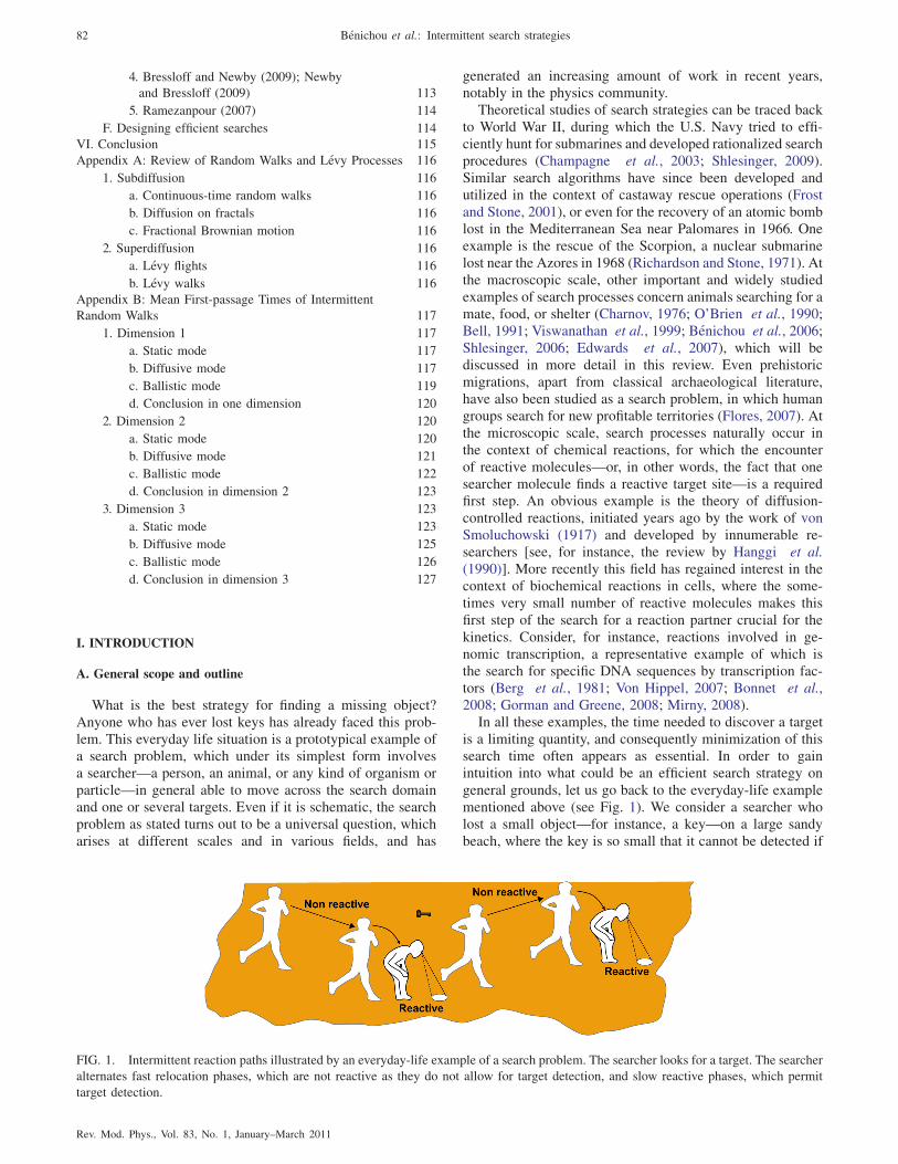
In all these examples, the time needed to discover a targetis a limiting quantity, and consequently minimization of thissearch time often appears as essential. In order to gainintuition into what could be an efficient search strategy ongeneral grounds, let us go back to the everyday-life examplementioned above (see Fig. 1). We consider a searcher wholost a small object—for instance, a key—on a large sandybeach, where the key is so small that it cannot be detected if

FIG. 1. Intermittent reaction paths illustrated by an everyday-life example of a search problem. The searcher looks for a target. The searcher

alternates fast relocation phases, which are not reactive as they do not allow for target detection, and slow reactive phases, which permit

target detection.

82 Benichou et al.: Intermittent search strategies

Rev. Mod. Phys., Vol. 83, No. 1, January–March 2011

the searcher passes by too fast. In addition, we assume thatthe searcher has no prior information on the position of thekey, except that the key is in a bounded domain (the beach).What is then the best strategy for the searcher to find the keyas fast as possible? A first strategy consists in a slow andcareful exploration (to make sure that the key will be detectedupon encounter) of the sand all along the beach. In the case ofa very large beach, the search time can then be very long. Analternative strategy consists in interrupting the slow and care-ful exploration of the sand by displacement phases, duringwhich the searcher relocates on the beach very fast, butwithout even trying to detect the key (typically the searcher‘‘runs’’). Hereafter the term ‘‘intermittent search strategies’’is used for such processes that combine two distinct phases: aphase of slow displacement that enables target detection, anda phase of faster motion during which the target cannot bedetected [note that the word ‘‘intermittent’’ has also beenused recently by Bartumeus (2009) with another definition].

The efficiency of such intermittent strategies results from atrade-off between speed and detection and can be qualita-tively discussed. Intuitively, the advantage of the fast reloca-tion phases for the searcher is to reach unvisited regions.The drawback is, however, that during these phases timeis consumed without any chance of detecting the target.Determination of the net efficiency of this strategy is there-fore not trivial, and in recent years many works have focusedon the following questions: (i) Can phases of fast motion thatdisable detection make the global search more efficient? (ii) Ifso, is there an optimal way for the searcher to share the timebetween the two phases? (iii) Are these intermittent searchpatterns relevant to the description of real situations?

The goal of this article is to review these works whilegiving explicit answers to these questions. More precisely, itis first shown that intermittent transport patterns are actuallywidely observed at various scales. At the macroscopic scale,this is, for example, the case of foraging animals (see Sec. II);at the microscopic scale, intermittent transport patterns areshown to be involved in the reaction pathway of DNA-binding proteins as well as in intracellular transport (seeSec. III). Second, generic stochastic models are used toshow that intermittent strategies are efficient strategies thatallow minimization of the search time (see Secs. II, III, andIV), and therefore suggest that this efficiency might justifytheir frequent observation in nature. Last, beyond these mod-eling aspects, it is proposed that intermittent strategies couldalso be used in a broader context to design and acceleratesearch processes.

B. General framework and first definitions

The search problem can take multiple forms (da Luz et al.,2009); in this section we define more precisely the frameworkof this review—namely, random intermittent search strat-egies—and introduce the main hypothesis that will be made.

1. Searching with or without cues

Although in essence in a search problem the target locationis unknown and cannot be found from a rapid inspection ofthe search domain, in practical cases there are often cues thatrestrict the territory to be explored or give indications of how

to explore it. A classical example is chemotaxis (Berg, 2004),which keeps raising interest in the biological and physicalcommunities [see, for example, Park et al. (2003), Kafri andDa Silveira (2008), and Tailleur and Cates (2008)]. Bacterialike E. coli swim with a succession of ‘‘runs’’ (approximatelystraight moves) and ‘‘tumbles’’ (random changes of direc-tion). When they sense a gradient of chemical concentration,they swim up or down the gradient by adjusting their tum-bling rate: When the environment is becoming more favor-able, they tumble less, whereas they tumble more when theirenvironment is degrading. This behavior results in a biastoward the most favorable locations of high concentrationof chemoattractant, which can be as varied as, for example,salts, glucose, amino acids, or oxygen. Recently it has beenshown that a similar behavior can also be triggered by otherkinds of external signal such as temperature gradients (Maedaet al., 1976; Salman et al., 2006; Salman and Libchaber,2007) or light intensity (Sprenger et al., 1993).

Chemotactic search requires a well-defined gradient ofchemoattractant and is therefore applicable only when theconcentration of cues is sufficient. In contrast, at low con-centrations cues can be sparse, or even discrete signals that donot allow for a gradient-based strategy. This is, for example,the case of animals sensing odors in air or water, where themixing in the potentially turbulent flow breaks up the chemi-cal signal into random and disconnected patches of highconcentration. Vergassola et al. (2007) proposed a searchalgorithm, which they called ‘‘infotaxis,’’ designed to work inthis case of sparse and fluctuating cues. This algorithm, basedon a maximization of the expected rate of information gain,produces trajectories such as ‘‘zigzagging’’ and ‘‘casting’’paths, which are similar to those observed in the flight ofmoths (Balkovsky and Shraiman, 2002).

This review focuses on the extreme case where no cue ispresent that could lead the searcher to the target. This as-sumption applies to targets that can be detected only if thesearcher is within a given detection radius a which is muchsmaller than the typical extension of the search domain. Inparticular, this assumption covers the case of search problemsat the scale of chemical reactions and, more generally, thecase of searchers whose motion is independent of any exteriorcue that could be emitted by the target.

2. Systematic versus random strategies

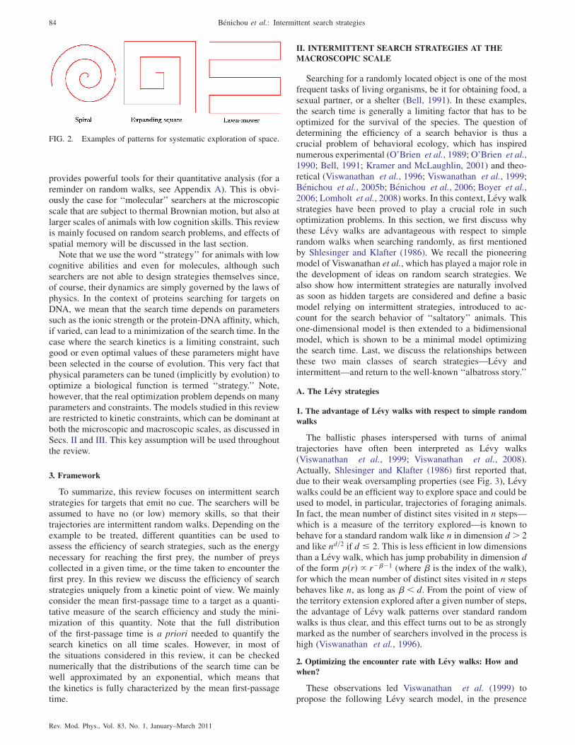
Whatever the scale, the behavior of a searcher reliesstrongly on its ability, or incapability, to keep memories ofits past explorations. Depending on the searcher and on thespace to be explored, this kind of spatial memory can playa more or less important role (Moreau et al., 2009). In anextreme case the searcher, for instance, human or animal, canhave a mental map of the exploration space and can thusperform a systematic search. Figure 2 presents several sys-tematic patterns: lawn mower, expanding square, and spiral[for more patterns, see, for example, Champagne et al.(2003)]. These types of searches have been extensivelystudied, in particular, for designing an efficient search oper-ated by humans (Dobbie, 1968; Stone, 1989).

In the opposite case where the searcher has low—orno—spatial memory abilities the search trajectories can bequalified as random, and the theory of stochastic processes

Benichou et al.: Intermittent search strategies 83


provides powerful tools for their quantitative analysis (for areminder on random walks, see Appendix A). This is obvi-ously the case for ‘‘molecular’’ searchers at the microscopicscale that are subject to thermal Brownian motion, but also atlarger scales of animals with low cognition skills. This reviewis mainly focused on random search problems, and effects ofspatial memory will be discussed in the last section.

Note that we use the word ‘‘strategy’’ for animals with lowcognitive abilities and even for molecules, although suchsearchers are not able to design strategies themselves since,of course, their dynamics are simply governed by the laws ofphysics. In the context of proteins searching for targets onDNA, we mean that the search time depends on parameterssuch as the ionic strength or the protein-DNA affinity, which,if varied, can lead to a minimization of the search time. In thecase where the search kinetics is a limiting constraint, suchgood or even optimal values of these parameters might havebeen selected in the course of evolution. This very fact thatphysical parameters can be tuned (implicitly by evolution) tooptimize a biological function is termed ‘‘strategy.’’ Note,however, that the real optimization problem depends on manyparameters and constraints. The models studied in this revieware restricted to kinetic constraints, which can be dominant atboth the microscopic and macroscopic scales, as discussed inSecs. II and III. This key assumption will be used throughoutthe review.

3. Framework

To summarize, this review focuses on intermittent searchstrategies for targets that emit no cue. The searchers will beassumed to have no (or low) memory skills, so that theirtrajectories are intermittent random walks. Depending on theexample to be treated, different quantities can be used toassess the efficiency of search strategies, such as the energynecessary for reaching the first prey, the number of preyscollected in a given time, or the time taken to encounter thefirst prey. In this review we discuss the efficiency of searchstrategies uniquely from a kinetic point of view. We mainlyconsider the mean first-passage time to a target as a quanti-tative measure of the search efficiency and study the mini-mization of this quantity. Note that the full distributionof the first-passage time is a priori needed to quantify thesearch kinetics on all time scales. However, in most ofthe situations considered in this review, it can be checkednumerically that the distributions of the search time can bewell approximated by an exponential, which means thatthe kinetics is fully characterized by the mean first-passagetime.

II. INTERMITTENT SEARCH STRATEGIES AT THE

MACROSCOPIC SCALE

Searching for a randomly located object is one of the mostfrequent tasks of living organisms, be it for obtaining food, asexual partner, or a shelter (Bell, 1991). In these examples,the search time is generally a limiting factor that has to beoptimized for the survival of the species. The question ofdetermining the efficiency of a search behavior is thus acrucial problem of behavioral ecology, which has inspirednumerous experimental (O’Brien et al., 1989; O’Brien et al.,1990; Bell, 1991; Kramer and McLaughlin, 2001) and theo-retical (Viswanathan et al., 1996; Viswanathan et al., 1999;Benichou et al., 2005b; Benichou et al., 2006; Boyer et al.,2006; Lomholt et al., 2008) works. In this context, Levy walkstrategies have been proved to play a crucial role in suchoptimization problems. In this section, we first discuss whythese Levy walks are advantageous with respect to simplerandom walks when searching randomly, as first mentionedby Shlesinger and Klafter (1986). We recall the pioneeringmodel of Viswanathan et al., which has played a major role inthe development of ideas on random search strategies. Wealso show how intermittent strategies are naturally involvedas soon as hidden targets are considered and define a basicmodel relying on intermittent strategies, introduced to ac-count for the search behavior of ‘‘saltatory’’ animals. Thisone-dimensional model is then extended to a bidimensionalmodel, which is shown to be a minimal model optimizingthe search time. Last, we discuss the relationships betweenthese two main classes of search strategies—Levy andintermittent—and return to the well-known ‘‘albatross story.’’

A. The Levy strategies

1. The advantage of Levy walks with respect to simple random

walks

The ballistic phases interspersed with turns of animaltrajectories have often been interpreted as Levy walks(Viswanathan et al., 1999; Viswanathan et al., 2008).Actually, Shlesinger and Klafter (1986) first reported that,due to their weak oversampling properties (see Fig. 3), Levywalks could be an efficient way to explore space and could beused to model, in particular, trajectories of foraging animals.In fact, the mean number of distinct sites visited in n steps—which is a measure of the territory explored—is known tobehave for a standard random walk like n in dimension d > 2and like nd=2 if d � 2. This is less efficient in low dimensionsthan a Levy walk, which has jump probability in dimension dof the form pðrÞ / r��1 (where � is the index of the walk),for which the mean number of distinct sites visited in n stepsbehaves like n, as long as �< d. From the point of view ofthe territory extension explored after a given number of steps,the advantage of Levy walk patterns over standard randomwalks is thus clear, and this effect turns out to be as stronglymarked as the number of searchers involved in the process ishigh (Viswanathan et al., 1996).

2. Optimizing the encounter rate with Levy walks: How and

when?

These observations led Viswanathan et al. (1999) topropose the following Levy search model, in the presence

FIG. 2. Examples of patterns for systematic exploration of space.



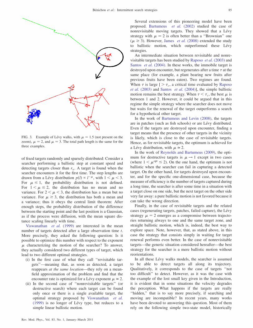
of fixed targets randomly and sparsely distributed: Consider asearcher performing a ballistic step at constant speed anddetecting targets closer than rv. A target is found when thesearcher encounters it for the first time. The step lengths aredrawn from a Levy distribution pðlÞ / l��, with 1<�< 3.For � � 1, the probability distribution is not defined.For 1<� � 2, the distribution has no mean and novariance. For 2<�< 3, the distribution has a mean but novariance. For � � 3, the distribution has both a mean anda variance; thus it obeys the central limit theorem: Afterenough steps, the probability distribution of the differencebetween the starting point and the last position is a Gaussian,as if the process were diffusion, with the mean square dis-tance scaling linearly with time.

Viswanathan et al. (1999) are interested in the meannumber of targets detected after a large observation time t.More precisely, they asked the following question: Is itpossible to optimize this number with respect to the exponent

� characterizing the motion of the searcher? To answer,they actually considered two different types of target, whichlead to two different optimal strategies.

(i) In the first case of what they call ‘‘revisitable tar-

gets’’—meaning that, as soon as detected, a targetreappears at the same location—they rely on a mean-field approximation of the problem and find that theencounter rate is optimized for a Levy exponent � ’ 2.

(ii) In the second case of ‘‘nonrevisitable targets’’ (ordestructive search) where each target can be foundonly once or there is a single available target, theoptimal strategy proposed by Viswanathan et al.(1999) is no longer of Levy type, but reduces to asimple linear ballistic motion.

Several extensions of this pioneering model have been

proposed. Bartumeus et al. (2002) studied the case of

nonrevisitable moving targets. They showed that a Levy

strategy with � ¼ 2 is often better than a ‘‘Brownian’’ one

(� � 3). However, James et al. (2008) extended the study

to ballistic motion, which outperformed these Levy

strategies.An intermediate situation between revisitable and nonre-

visitable targets has been studied by Raposo et al. (2003) and

Santos et al. (2004). In these works, the immobile target is

destroyed upon encounter, but regenerates after a time � at thesame place (for example, a plant bearing new fruits after

previous fruits have been eaten). Two regimes are found.

When � is large [> �c, a critical time evaluated by Raposo

et al. (2003) and Santos et al. (2004)], the simple ballistic

motion remains the best strategy. When � < �c, the best � is

between 1 and 2. However, it could be argued that in this

regime the simple strategy where the searcher does not move

but waits for the renewal of the target outperforms a search

for a hypothetical other target.In the work of Bartumeus and Levin (2008), the targets

are in patches (such as fish schools) or are Levy distributed.

Even if the targets are destroyed upon encounter, finding a

target means that the presence of other targets in the vicinity

is likely, which is close to the case of revisitable targets.

Hence, as for revisitable targets, the optimum is achieved for

a Levy distribution, with � ’ 2.In the work of Reynolds and Bartumeus (2009), the opti-

mum for destructive targets is � ! 1 except in two cases

(where 1<�opt � 2). On the one hand, the optimum is not

ballistic when the searcher can fail in capturing a detected

target. On the other hand, for targets destroyed upon encoun-

ter, and for the specific one-dimensional case, because the

measure of efficiency is the number of targets captured during

a long time, the searcher is after some time in a situation with

a target close on one side, but the next target on the other side

very far away: a pure ballistic motion is not favored because it

can take the wrong direction.Finally, in the case of revisitable targets and the related

cases (regenerating targets, patches, failed capture), the Levy

strategy � ¼ 2 emerges as a compromise between trajecto-

ries returning always to one and the same target zone, and

straight ballistic motion, which is, indeed, the best way to

explore space. Note, however, that, as stated above, in this

case the strategy that consists simply in waiting for target

renewal performs even better. In the case of nonrevisitable

targets—the generic situation considered hereafter—the best

strategy for the searcher is a mere ballistic motion without

reorientations.In all these Levy walks models, the searcher is assumed

to be able to detect targets all along its trajectory.

Qualitatively, it corresponds to the case of targets ‘‘not

too difficult’’ to detect. However, as it was the case with

the example of the lost small key given in the Introduction,

it is evident that in some situations the velocity degrades

the perception. What happens if the targets are really

‘‘hidden,’’ that is to say more precisely, if searching and

moving are incompatible? In recent years, many works

have been devoted to answering this question. Most of them

rely on the following simple two-state model, historically

FIG. 3. Example of Levy walks, with � ¼ 1:5 (not present on the

zoom), � ¼ 2, and � ¼ 3. The total path length is the same for the

three examples.



introduced to account for the search behavior of the ‘‘salta-tory animals.’’

B. A basic model of intermittence

1. Observations: The case of saltatory animals

Anyone who has ever lost keys knows that an intermittentbehavior combining local scanning phases and relocatingphases is often adopted instinctively. Indeed, numerous stud-ies of foraging behavior of a broad range of animal speciesshow that such intermittent behavior is commonly observedand that the durations of search and displacement phasesvary widely (O’Brien et al., 1990; Bell, 1991; Kramer andMcLaughlin, 2001). The spectrum, which goes from cruisestrategy (for large fishes that swim continuously, such as tuna)to ambush or sit-and-wait search, where the forager remainsstationary for long periods (such as a rattlesnake), has re-mained uninterpreted for a long time. As explained in theIntroduction, the interest of this type of intermittent strategy,often referred to as ‘‘saltatory’’ (O’Brien et al., 1990; Kramerand McLaughlin, 2001) in the context of foraging animals,can be understood intuitively when the targets are ‘‘difficult’’to detect and sparsely distributed, as is the case for manyforagers (such as ground foraging birds, lizards, planktivo-rous fish1): Since a fast movement is known to significantlydegrade perception abilities (O’Brien et al., 1990; Kramerand McLaughlin, 2001), the forager must search slowly.Then, it has to relocate as fast as possible in order to explorea previously unscanned space, and search slowly again.

Even though numerous models based on optimizationof the net energy gain (Knoppien and Reddingius, 1985;O’Brien et al., 1989; Anderson et al., 1997) predict anoptimal strategy for foragers, the large number of unknownparameters used to model the complexity of the energeticconstraints renders a quantitative comparison with experi-mental data difficult. In the model presented in this section,the search time is assumed to be the relevant quantity opti-mized by the forager in order to obtain a sufficient dailyamount of food and to precede other competing foragers. Theenergy cost is treated only as an external constraint that setsthe maximal speed of the animal. As explained in the nextsections, this purely kinetic model of target search capturesthe essential features of saltatory search behavior observedfor foragers in experiments (Kramer and McLaughlin, 2001),when the predator has no information about the prey location.

2. Model

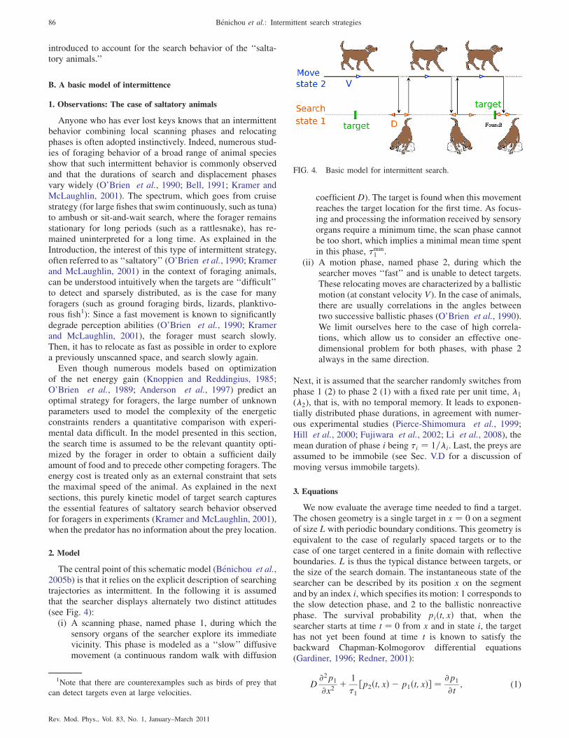
The central point of this schematic model (Benichou et al.,2005b) is that it relies on the explicit description of searchingtrajectories as intermittent. In the following it is assumedthat the searcher displays alternately two distinct attitudes(see Fig. 4):

(i) A scanning phase, named phase 1, during which thesensory organs of the searcher explore its immediatevicinity. This phase is modeled as a ‘‘slow’’ diffusivemovement (a continuous random walk with diffusion

coefficient D). The target is found when this movementreaches the target location for the first time. As focus-ing and processing the information received by sensoryorgans require a minimum time, the scan phase cannotbe too short, which implies a minimal mean time spentin this phase, �min

1 .

(ii) A motion phase, named phase 2, during which thesearcher moves ‘‘fast’’ and is unable to detect targets.These relocating moves are characterized by a ballisticmotion (at constant velocity V). In the case of animals,there are usually correlations in the angles betweentwo successive ballistic phases (O’Brien et al., 1990).We limit ourselves here to the case of high correla-tions, which allow us to consider an effective one-dimensional problem for both phases, with phase 2always in the same direction.

Next, it is assumed that the searcher randomly switches fromphase 1 (2) to phase 2 (1) with a fixed rate per unit time, �1

(�2), that is, with no temporal memory. It leads to exponen-tially distributed phase durations, in agreement with numer-ous experimental studies (Pierce-Shimomura et al., 1999;Hill et al., 2000; Fujiwara et al., 2002; Li et al., 2008), themean duration of phase i being �i ¼ 1=�i. Last, the preys areassumed to be immobile (see Sec. V.D for a discussion ofmoving versus immobile targets).

3. Equations

We now evaluate the average time needed to find a target.The chosen geometry is a single target in x ¼ 0 on a segmentof size Lwith periodic boundary conditions. This geometry isequivalent to the case of regularly spaced targets or to thecase of one target centered in a finite domain with reflectiveboundaries. L is thus the typical distance between targets, orthe size of the search domain. The instantaneous state of thesearcher can be described by its position x on the segmentand by an index i, which specifies its motion: 1 corresponds tothe slow detection phase, and 2 to the ballistic nonreactivephase. The survival probability piðt; xÞ that, when thesearcher starts at time t ¼ 0 from x and in state i, the targethas not yet been found at time t is known to satisfy thebackward Chapman-Kolmogorov differential equations(Gardiner, 1996; Redner, 2001):

D@2p1

@x2þ 1

�1½p2ðt; xÞ � p1ðt; xÞ� ¼ @p1

@t; (1)

FIG. 4. Basic model for intermittent search.

1Note that there are counterexamples such as birds of prey that

can detect targets even at large velocities.



� V@p2

@xþ 1

�2½p1ðt; xÞ � p2ðt; xÞ� ¼ @p2

@t: (2)

Since tiðxÞ, the mean first-passage time at the target, startingfrom x in phase i, is given by

tiðxÞ ¼ �Z 1

0t@piðt; xÞ

@tdt ¼

Z 1

0piðt; xÞdt; (3)

it is easily found from Eqs. (1) and (2) to satisfy

Dd2t1dx2

þ 1

�1½t2ðxÞ � t1ðxÞ� ¼ �1; (4)

� Vdt2dx

þ 1

�2½t1ðxÞ � t2ðxÞ� ¼ �1: (5)

These differential equations have to be completed by bound-ary conditions. Since we have periodic boundary conditionsand the target at x ¼ 0 can be found only in state 1, we gett1ð0Þ ¼ t1ðLÞ ¼ 0, t2ð0Þ ¼ t2ðLÞ.

4. Results

The average search time hti is defined as the average oft1ðxÞ over the initial position x of the searcher, which isuniformly distributed over the segment ½0; L�, as the searcherinitially does not know the target’s location. It is found to begiven by Benichou et al. (2005b):

hti¼ ð�2þ�1Þ0@L2

ðe�þ��1Þ ffiffiffiffiffiffiffiffiffiffiffiffiffi1þ4r

p þð1þ2rÞðe��e�Þffiffiffiffiffiffiffiffiffiffiffiffiffi1þ4r

p ðe��1Þðe��1Þ�2V

�1

r�1

1A; (6)

with

r ¼ �22V2

D�1; (7)

� ¼ L

2

0@� 1

�2Vþ

ffiffiffiffiffiffiffiffiffiffiffiffiffiffiffiffiffiffiffiffiffiffiffiffiffiffiffiffiffi1

�22V2þ 4

1

D�1

s 1A; (8)

� ¼ �L

2

0@ 1

�2Vþ

ffiffiffiffiffiffiffiffiffiffiffiffiffiffiffiffiffiffiffiffiffiffiffiffiffiffiffiffiffi1

�22V2þ 4

1

D�1

s 1A: (9)

In the limit of L � V�2;ffiffiffiffiffiffiffiffiffiD�1

p; D�1=V�2, this simplifies:

hti ’ Lð�2 þ �1ÞðD�1 þ 2�22V2Þ

2�2VffiffiffiffiffiffiffiffiffiD�1

p ffiffiffiffiffiffiffiffiffiffiffiffiffiffiffiffiffiffiffiffiffiffiffiffiffiffiffiffiD�1 þ 4�22V

2q : (10)

Note that, because of intermittence, hti / L, whereas fordiffusion alone the mean detection time is tdiff ¼ L2=12D.Intermittence is thus favorable (meaning that the gain, de-fined as tdiff=hti is greater than 1), at least for L large enough.

Intermittence is favorable and the strategy can evenbe optimized. The mean search time is minimized for�opt1 ¼ �min

1 and �opt2 , satisfying the relation [see Benichou

et al. (2005c) for details]

�31 þ 6�21�

22

�� 8

�52�2

¼ 0; (11)

where � ¼ D=V2 is an extra characteristic time, dependingon the searcher’s characteristics. This minimum takes asimple form in two different regimes.

(i) If �1 � �, the minimum of the search time is for�1 ¼ �min

1 and

�opt2 ¼

�3��214

�1=3

: (12)

In this regime, denoted by ‘‘S’’ for ‘‘searching,’’ onehas �1 > �2: The searcher spends more time scanningthan moving.

(ii) If �1 � �, the minimum of the search time is for�1 ¼ �min

1 and

�opt2 ¼

��2�318

�1=5

: (13)

In this regime, denoted by ‘‘M’’ for ‘‘moving,’’ one has�1 < �2, which means that the searcher spends moretime moving than scanning.

5. Comparison with experimental data

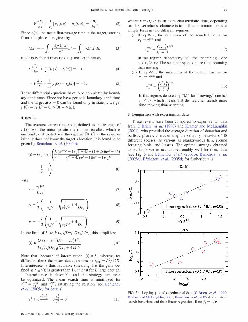
These results have been compared to experimental datafrom O’Brien et al. (1990) and Kramer and McLaughlin(2001), who provided the average duration of detection andballistic phases, characterizing the saltatory behavior of 18different species, as various as planktivorous fish, groundforaging birds, and lizards. The optimal strategy obtainedabove is shown to account reasonably well for these data[see Fig. 5 and Benichou et al. (2005b); Benichou et al.(2005c); Benichou et al. (2005d) for further details].

FIG. 5. Log-log plot of experimental data (O’Brien et al., 1990;

Kramer and McLaughlin, 2001; Benichou et al., 2005b) of saltatory

search behaviors and their linear regression. Here fi ¼ 1=�i.



These results show that the saltatory patterns observed area way to optimize the search, and that it is probably a reasonwhy this type of pattern is observed so often, as it could have

been favored by natural selection.

C. Two-dimensional intermittent search processes:

An alternative to Levy strategies

1. Motivation

The model of intermittent search presented previously was

one dimensional, with ballistic phases infinitely correlated, inthe sense that the direction taken is always the same. Here wepresent a model of intermittent search strategies in dimen-sion 2 (Benichou et al., 2006; Benichou et al., 2007), whichencompasses a much broader field of applications, in particu-

lar, for animal or human searchers. It is shown that bidimen-sional intermittent search strategies do optimize the searchtime for nonrevisitable targets, i.e., targets that are destroyedupon discovery (see Sec. II.A.2). The optimal way to share

the time between the phases of nonreactive displacementand of reactive search is explicitly determined. Technically,this approach relies on an approximate analytical solutionbased on a decoupling hypothesis, which proves to reproducequantitatively numerical simulations over a wide range of

parameters.

2. Model

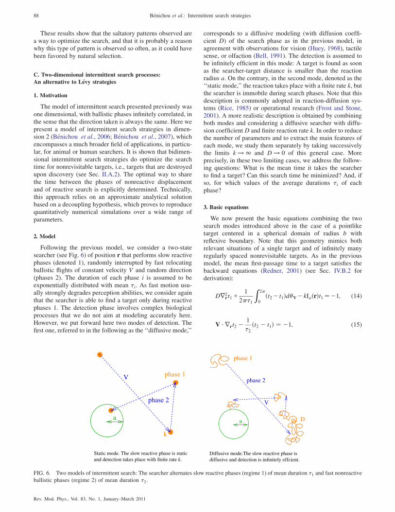
Following the previous model, we consider a two-statesearcher (see Fig. 6) of position r that performs slow reactivephases (denoted 1), randomly interrupted by fast relocatingballistic flights of constant velocity V and random direction

(phases 2). The duration of each phase i is assumed to beexponentially distributed with mean �i. As fast motion usu-ally strongly degrades perception abilities, we consider againthat the searcher is able to find a target only during reactive

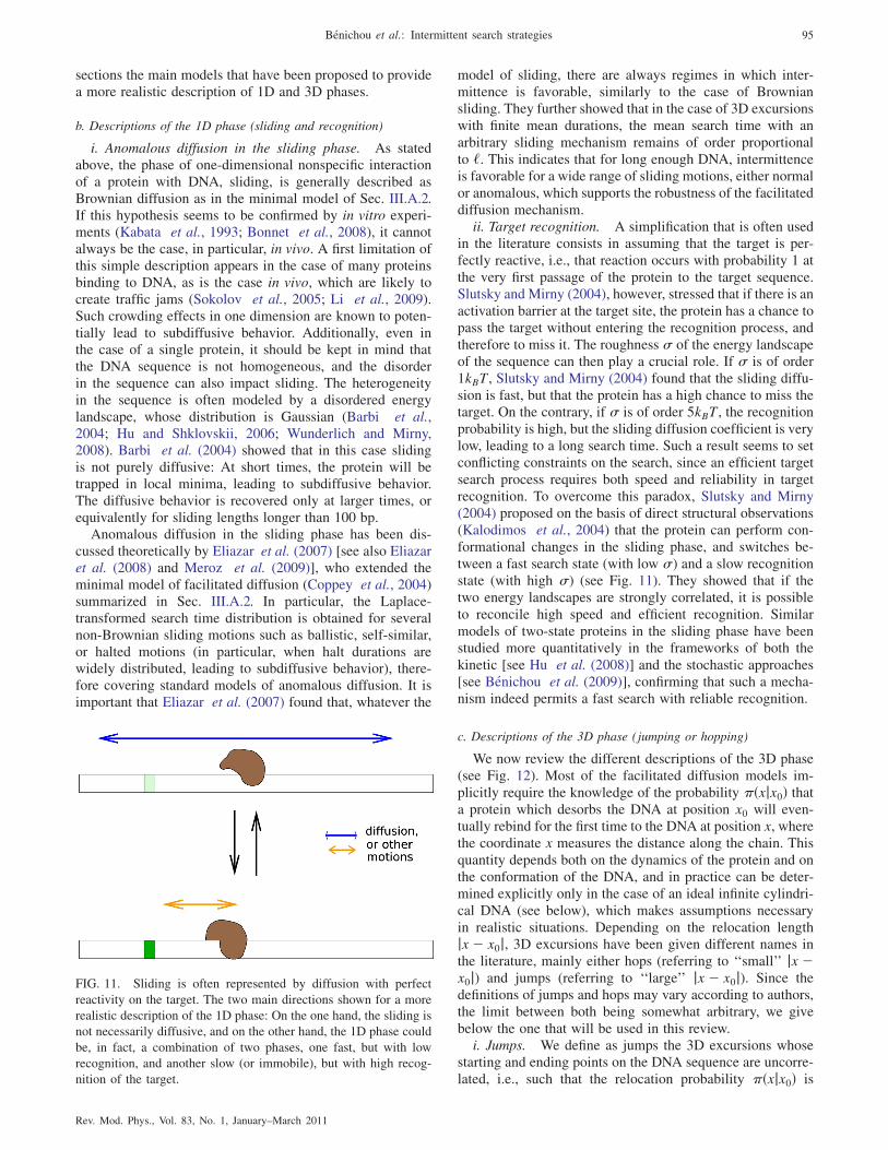
phases 1. The detection phase involves complex biologicalprocesses that we do not aim at modeling accurately here.However, we put forward here two modes of detection. Thefirst one, referred to in the following as the ‘‘diffusive mode,’’

corresponds to a diffusive modeling (with diffusion coeffi-cient D) of the search phase as in the previous model, inagreement with observations for vision (Huey, 1968), tactilesense, or olfaction (Bell, 1991). The detection is assumed tobe infinitely efficient in this mode: A target is found as soonas the searcher-target distance is smaller than the reactionradius a. On the contrary, in the second mode, denoted as the‘‘static mode,’’ the reaction takes place with a finite rate k, butthe searcher is immobile during search phases. Note that thisdescription is commonly adopted in reaction-diffusion sys-tems (Rice, 1985) or operational research (Frost and Stone,2001). A more realistic description is obtained by combiningboth modes and considering a diffusive searcher with diffu-sion coefficientD and finite reaction rate k. In order to reducethe number of parameters and to extract the main features ofeach mode, we study them separately by taking successivelythe limits k ! 1 and D ! 0 of this general case. Moreprecisely, in these two limiting cases, we address the follow-ing questions: What is the mean time it takes the searcherto find a target? Can this search time be minimized? And, ifso, for which values of the average durations �i of eachphase?

3. Basic equations

We now present the basic equations combining the twosearch modes introduced above in the case of a pointliketarget centered in a spherical domain of radius b withreflexive boundary. Note that this geometry mimics bothrelevant situations of a single target and of infinitely manyregularly spaced nonrevisitable targets. As in the previousmodel, the mean first-passage time to a target satisfies thebackward equations (Redner, 2001) (see Sec. IV.B.2 forderivation):

Dr2rt1þ 1

2��1

Z 2�

0ðt2� t1Þd�V�kIaðrÞt1¼�1; (14)

V � rrt2 � 1

�2ðt2 � t1Þ ¼ �1; (15)

phase 2

V

a

phase 1

k

Static mode. The slow reactive phase is static and detection takes place with finite rate k.

phase 2

V

phase 1

Da

Diffusive mode.The slow reactive phase isdiffusive and detection is infinitely effcient.

FIG. 6. Two models of intermittent search: The searcher alternates slow reactive phases (regime 1) of mean duration �1 and fast nonreactiveballistic phases (regime 2) of mean duration �2.



where t1 is the mean first-passage time starting from state 1 atposition r, and t2 is the mean first-passage time starting fromstate 2 at position r with velocity V, of direction character-ized by the angle �V . Here IaðrÞ ¼ 1 if jrj � a and IaðrÞ ¼ 0if jrj> a. In the present form, these integro-differentialequations do not seem to allow for an exact resolution withstandard methods. We thus resort to an approximate decou-pling scheme, which relies on the following idea. If thesearcher initially starts in phase 2, and if the target is close,its initial direction matters. But as soon as the initial positionis far from the target, there are numerous reorientationsbefore finding the target, implying that the initial directiondoes not matter. Consequently, if b � a and once the meansearch time has been averaged over the starting position, theeffect of the initial direction can be neglected. This allows usto make an approximation and solve the system [for moretechnical details, see Appendix B and Benichou et al. (2006);Benichou et al. (2007)].

4. Results for the diffusive mode of detection

For the diffusive mode of detection (k ! 1), an analyticalapproximation for the search time can be obtained (seeAppendix B). In the case of low target density (a � b),which is most relevant for hidden-target search problems,three regimes arise. In the first regime a � b � D=V, therelocating phases are not efficient and intermittence is use-less. In the second regime a � D=V � b, it can be shown(see Appendix A.2.b) that the intermittence can significantlyspeed up the search (typically by a factor of 2), but that it doesnot change the order of magnitude of the search time. On thecontrary, in the last regime D=V � a � b, the optimalstrategy, obtained for

�opt1 � D

2V2

ln2ðb=aÞ2 lnðb=aÞ � 1

;

�opt2 � a

V½lnðb=aÞ � 1=2�1=2;

(16)

leads to a search time arbitrarily smaller than the noninter-mittent search time when V ! 1. Note that this optimalstrategy corresponds to a scaling law

�opt1

�opt2

� D

a21

½2� 1= lnðb=aÞ�2 ; (17)

which does not depend on V.

5. Results for the static mode of detection

We now turn to the static mode (D ! 0) (seeAppendix B.1). In this case, intermittence is trivially neces-sary to find the target, and the optimization of the searchtime leads for b � a to

�1;min ¼�a

Vk

�1=2

�2 lnðb=aÞ � 1

8

�1=4

; (18)

�2;min ¼ a

V½lnðb=aÞ � 1=2�1=2; (19)

corresponding to the scaling law �2;min ¼ 2k�21;min, which still

does not depend on V.

6. Conclusion

This bidimensional two-state model of search processes fornonrevisitable targets closely relies on the experimentallyobserved intermittent strategies adopted by foraging animals.Using a decoupling approximation numerically validated, itcan be analytically solved, allowing us to draw several con-clusions. (i) The mean search time hti presents a globalminimum for finite values of the �i, which means that inter-mittent strategies constitute optimal strategies, as opposed toLevy walks, which are optimal only for revisitable targets.(ii) The optimal �

opt1 values obtained for two modes of

detection are different and depend explicitly on D and k,leading to different scaling laws that are susceptible to dis-criminate between the two search modes. (iii) A striking andnonintuitive feature is that both modes of search studied leadto the same optimal value of �

opt2 . As this optimal time does

not depend on the specific characteristics D and k of thesearch mode, it seems to constitute a general property ofintermittent search strategies. The robustness of these con-clusions will be discussed further in Sec. IV in the frameworkof a more general model.

D. Should foraging animals really adopt Levy strategies?

As seen before, intermittent strategies are an alternative toLevy walks (defined in Sec. II.A) for interpreting trajectoriesof foraging animals. However, the Levy walks are oftenthought to be optimal and widespread in nature. Is this reallytrue?

1. The albatross story

Many foraging animals, including albatrosses, deer, andbumblebees to name a few, have long been thought to adoptLevy strategies described in the pioneering work ofViswanathan et al. (1999). These foraging behaviors wererepeatedly accounted for by stating in the more generalframework of search processes that Levy walks are optimalsearch strategies, as they constitute the best way to explorespace. Recently Edwards et al. (2007) reanalyzed these data,completed by newly gathered data on foraging albatrosses,and showed that, in fact, there was no experimental evidencefor the Levy walk behavior.2 This study questions the inter-pretation of several experimental works, but also raises a newimportant and puzzling question: Why do animals not adoptthe Levy walk strategy which has, however, been reported tobe an optimal search strategy? Here we clarify this apparentlyparadoxical situation.

2. Do animals really perform Levy walks?

As the optimality of Levy strategies crucially requiresconditions on the targets (regenerated at the same place,

2Albatrosses’ behavior was followed by a humidity sensor on the

birds. Flights were taken as the ‘‘dry‘‘ phases, interspersed with

humid phases, when the birds touched the ocean. Very long

’’flights’’ eventually proved to be rest time, when the bird was in

its nest. Once these misinterpreted dry phases were removed, the

distribution of flights’ durations is no longer a power law.



patched, or not easily captured) and conditions on the

searcher (no switch when a target is found, which is a very

simple form of memory), it cannot be taken as a general rule

even if realistic for certain species. On the contrary, we argue

that the general question of determining the best strategy

for finding a single hidden target belongs to the situation

of destructive search, where, in the framework of the

Viswanathan et al. (1999) model, the most efficient way to

find a randomly hidden target is simply a linear ballistic

motion and not a Levy strategy (see Sec. II.A). As a conse-

quence, there is no paradox: The reason that Levy walks are

not observed in the work of Edwards et al. (2007) is probably

because they do not constitute robust optimal search

strategies.And what about other experimental observations? Among

experimental studies analyzing organisms’ trajectories as a

succession of segments interspersed with turns, an important

proportion reports times between turns distributed exponen-

tially [a list of examples, far from exhaustive: C. Elegans

worm (Pierce-Shimomura et al., 1999; Fujiwara et al.,

2002), fish (Hill et al., 2000), plankton in some of the

conditions studied by Bartumeus et al. (2003), amoebae

(Li et al., 2008), etc.]. However, apart from the controversial

albatross study (Edwards et al., 2007), there is a boom in

articles claiming that Levy behavior is observed for some

animal species. Some of them can be dismissed as evidence

of Levy behavior. On the one hand, as explained in detail in

Edwards et al. (2007), due to experimental limitations, most

data cover only a very limited range, which makes difficult a

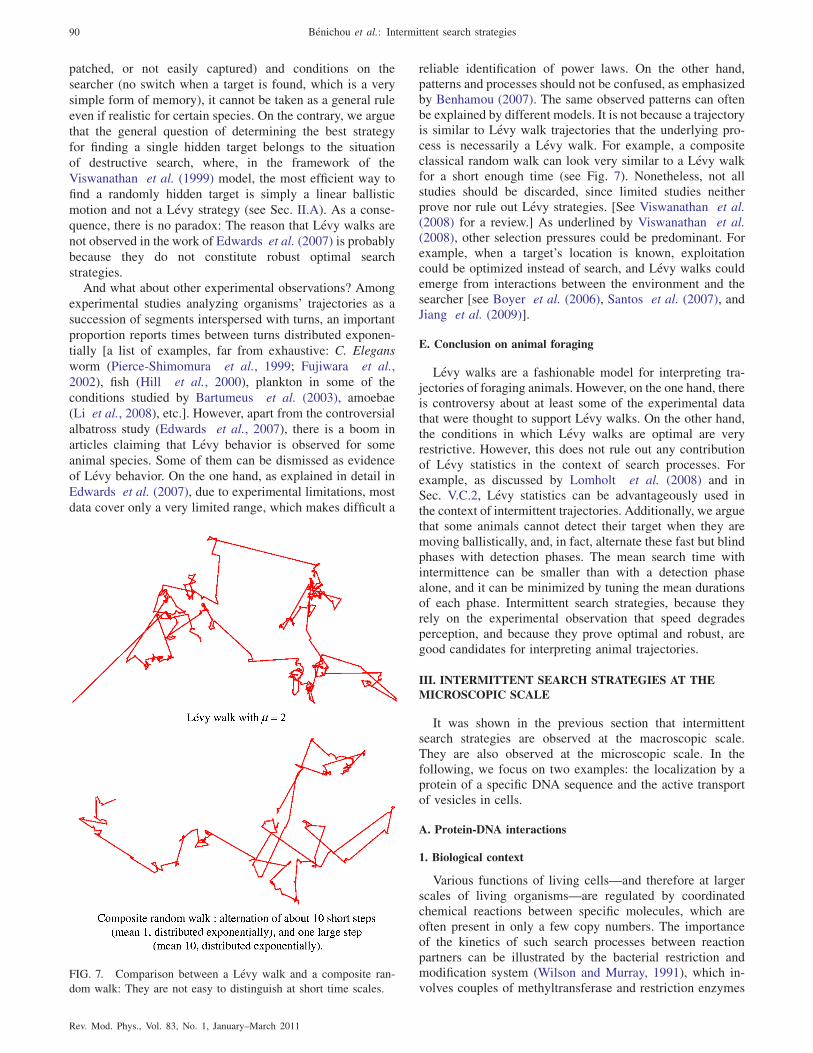
reliable identification of power laws. On the other hand,patterns and processes should not be confused, as emphasizedby Benhamou (2007). The same observed patterns can oftenbe explained by different models. It is not because a trajectoryis similar to Levy walk trajectories that the underlying pro-cess is necessarily a Levy walk. For example, a compositeclassical random walk can look very similar to a Levy walkfor a short enough time (see Fig. 7). Nonetheless, not allstudies should be discarded, since limited studies neitherprove nor rule out Levy strategies. [See Viswanathan et al.(2008) for a review.] As underlined by Viswanathan et al.(2008), other selection pressures could be predominant. Forexample, when a target’s location is known, exploitationcould be optimized instead of search, and Levy walks couldemerge from interactions between the environment and thesearcher [see Boyer et al. (2006), Santos et al. (2007), andJiang et al. (2009)].

E. Conclusion on animal foraging

Levy walks are a fashionable model for interpreting tra-jectories of foraging animals. However, on the one hand, thereis controversy about at least some of the experimental datathat were thought to support Levy walks. On the other hand,the conditions in which Levy walks are optimal are veryrestrictive. However, this does not rule out any contributionof Levy statistics in the context of search processes. Forexample, as discussed by Lomholt et al. (2008) and inSec. V.C.2, Levy statistics can be advantageously used inthe context of intermittent trajectories. Additionally, we arguethat some animals cannot detect their target when they aremoving ballistically, and, in fact, alternate these fast but blindphases with detection phases. The mean search time withintermittence can be smaller than with a detection phasealone, and it can be minimized by tuning the mean durationsof each phase. Intermittent search strategies, because theyrely on the experimental observation that speed degradesperception, and because they prove optimal and robust, aregood candidates for interpreting animal trajectories.

III. INTERMITTENT SEARCH STRATEGIES AT THE

MICROSCOPIC SCALE

It was shown in the previous section that intermittentsearch strategies are observed at the macroscopic scale.They are also observed at the microscopic scale. In thefollowing, we focus on two examples: the localization by aprotein of a specific DNA sequence and the active transportof vesicles in cells.

A. Protein-DNA interactions

1. Biological context

Various functions of living cells—and therefore at largerscales of living organisms—are regulated by coordinatedchemical reactions between specific molecules, which areoften present in only a few copy numbers. The importanceof the kinetics of such search processes between reactionpartners can be illustrated by the bacterial restriction andmodification system (Wilson and Murray, 1991), which in-volves couples of methyltransferase and restriction enzymes

FIG. 7. Comparison between a Levy walk and a composite ran-

dom walk: They are not easy to distinguish at short time scales.



that recognize the same sequence on DNA [for example,

EcoRV recognizes the sequence GATATC (Taylor and

Halford, 1989)]. Methyltransferase enzymes methylate this

specific sequence on the bacterial DNA in order to protect it

from restriction enzymes, whose function is the opposite—to

cut the DNA at this specific sequence. This function is first

aimed at impairing any intruder viral DNA that enters the cell

and that is very likely to contain the target sequence. Indeed,

this sequence, typically 4–8 base pairs, is very short as

compared to the viral genome, which, depending on the virus,

can be made of 103–106 base pairs (typically 5 104 for

bacteriophages). The infected bacterium then faces a vital

search problem: Restriction enzymes must find their target

sequence on the viral DNA reliably to inactivate the virus

before it exploits the bacteria machinery and kills it.More generally, it is well established that some sequence-

specific proteins find their target site in a remarkably short

time. For the lac repressor, for example, Riggs et al. (1970)

measured association rates orders of magnitude larger than

those expected for reactions limited by the classical three-

dimensional diffusion [results confirmed by Hsieh and

Brenowitz (1997) at different salt concentrations, ruling out

electrostatic effects as the only explanation]. Halford (2009)

argued that, in fact, only a few enzymes react significantly

faster than the three-dimensional (3D) diffusion limit.

However, this study underlined that many enzymes react at

rates close to the diffusion limit, and that this observation is

still impressive. Indeed, classical experiments are performed

with a considerable excess of DNA, which is likely to contain

sequences similar to the target sequence which therefore

act as traps, slowing down the enzymes in their search. In a

series of seminal articles, Berg et al. (1981), Winter and Von

Hippel (1981), and Winter et al. (1981), proposed that 3D

diffusion (or ‘‘hopping’’ or ‘‘jumping’’) was not the only

motion available to the protein, even if no energy is consumed

(unlike some enzymes, which consume energy to scan the

DNA molecule sequentially). They suggested that, in some

cases, proteins could bind nonspecifically to DNA due to a

weak electrostatic interaction and diffuse along the chain

in a process named sliding [see Von Hippel (2007) and

Dahirel et al. (2009)] for more details on the weak electro-

static interaction). It was then argued that the combination of

sliding and 3D diffusion, i.e., facilitated diffusion, can make

the search for a sequence two orders of magnitude faster than

3D diffusion alone and henceforth sufficiently efficient [see

also Adam and Delbruck (1968)].This search mechanism actually can be classified as inter-

mittent, in the general meaning defined in the Introduction.

Indeed, on the one hand, three-dimensional diffusion off the

DNA molecule is fast, but it does not allow for target detec-

tion. On the other hand, sliding is a phase of motion along

DNA, which therefore enables target detection, but which is

much slower due to a higher effective friction.The pioneering studies on facilitated diffusion (Riggs

et al., 1970; Berg et al., 1981; Winter et al., 1981; Winter

and Von Hippel, 1981) are based on ensemble measurements,

which were for a long time the only way to experimentally

access protein-DNA interactions. Recently developed tech-

niques make possible the observation of this interaction at the

level of a single molecule, with a resolution in space and time

still improving [for a review on the experimental results, see

Gorman and Greene (2008)]. It is now confirmed directly

that many proteins searching for a specific sequence on DNA

combine hopping or jumping and sliding (see Fig. 8). Sliding

phases have been clearly identified [both in vitro (Kabata

et al., 1993) and in vivo (Bakk and Metzler, 2004; Wang

et al., 2006; Elf et al., 2007)], as well as hopping or jumping

phases (Gowers et al., 2005; Bonnet et al., 2008; Komazin-

Meredith et al., 2008; van den Broek et al., 2008).With these new single-molecule experiments, theoretical

models have bloomed too. First, we present here a stochastic

approach to a simplified version of the problem, which shows

that it is the intermittent nature of the trajectories that makes

possible such high reaction rates. This minimal model per-

mits one to calculate explicitly the mean search time for such

intermittent reaction paths and shows that reactivity can even

be optimized by properly tuning simple dynamic parameters

of intermittent trajectories. Next, we discuss the different

directions of extension of recent theoretical models.

2. Minimal model of intermittent reaction paths

We present here a simple model of intermittent reaction

paths with minimal ingredients (Coppey et al., 2004). We

first define the model, then explain the main steps of the

calculation, and eventually give the results.

a. Definition of the model

We consider a generic protein searching for its target site

on a DNAmolecule (see Fig. 9). The pathway followed by the

protein, considered as a pointlike particle, is a succession of

1D diffusions along the DNA strand (sliding phases denoted

phases 1) and 3D excursions in the surrounding solution

FIG. 8. Artistic view of a DNA-protein interaction, which com-

bines one-dimensional sliding phases and three-dimensional relo-

cation phases. From Virginie Denis, Pour la Science 352, February

2007.



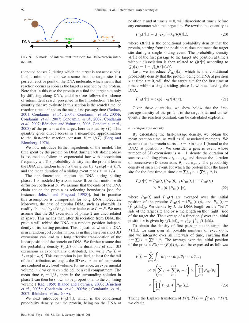
(denoted phases 2, during which the target is not accessible).In this minimal model we assume that the target site is aperfect reactive point of the DNAmolecule, which means thatreaction occurs as soon as the target is reached by the protein.Note that in this case the protein can find the target site onlyby diffusing along DNA, and therefore follows the schemeof intermittent search presented in the Introduction. The keyquantity that we evaluate in this section is the search time, orreaction time, defined as the mean first-passage time (Redner,2001; Condamin et al., 2005a; Condamin et al., 2005b;Condamin et al., 2007; Condamin et al., 2007; Condaminet al., 2007; Benichou and Voituriez, 2008; Condamin et al.,2008) of the protein at the target, here denoted by hTi. Thisquantity gives direct access in a mean-field approximationto the first-order reaction constant K ¼ 1=hTi (Berg andBlomberg, 1976).

We now introduce further ingredients of the model. Thetime spent by the protein on DNA during each sliding phaseis assumed to follow an exponential law with dissociationfrequency �1. The probability density that the protein leavesthe DNA at a random time t is then given by �1 expð��1tÞdt,and the mean duration of a sliding event reads �1 ¼ 1=�1.

The one-dimensional motion on DNA during slidingphases 1 is modeled by a continuous Brownian motion withdiffusion coefficient D. We assume that the ends of the DNAchain act on the protein as reflecting boundaries [see, forinstance, Jeltsch and Pingoud (1998)], but in practicethis assumption is unimportant for long DNA molecules.Moreover, the case of circular DNA, such as plasmids, isreadily obtained by taking the particular case L ¼ R. We nextassume that the 3D excursions of phase 2 are uncorrelatedin space. This means that, after dissociation from DNA, theprotein will rebind the DNA at a random position indepen-dently of its starting position. This is justified when the DNAis in a random coil conformation, as in this case even short 3Dexcursions can lead to a long effective translocation of thelinear position of the protein on DNA. We further assume thatthe probability density P3DðtÞ of the duration t of such 3Dexcursions is exponentially distributed, and write P3DðtÞ ¼�2 expð��2tÞ. This assumption is justified, at least for the tailof the distribution, as long as the 3D excursions of the proteinare confined in a closed volume, for instance, an experimentalvolume in vitro or in vivo the cell or a cell compartment. Themean time �2 ¼ 1=�2 spent in the surrounding solution inphase 2 can then be shown to be proportional to the confiningvolume ( Kac, 1959; Blanco and Fournier, 2003; Benichouet al., 2005a; Condamin et al., 2005a; ; Condamin et al.,2007; Benichou et al., 2008).

We next introduce P1DðtjxÞ, which is the conditionalprobability density that the protein, being on the DNA at

position x and at time t ¼ 0, will dissociate at time t beforeany encounter with the target site. We rewrite this quantity as

P1DðtjxÞ ¼ �1 expð��1tÞQðtjxÞ; (20)

where QðtjxÞ is the conditional probability density that theprotein, starting from the position x, does not meet the targetsite during a single sliding event. The probability densityjðtjxÞ of the first passage to the target site position at time twithout dissociation is then related to QðtjxÞ according toQðtjxÞ ¼ 1� R

t0 jðt0jxÞdt0.

Last, we introduce �P1DðtjxÞ, which is the conditionalprobability density that the protein, being on DNA at positionx at time t ¼ 0, will find the target site for the first time attime t within a single sliding phase 1, without leaving theDNA:

�P1DðtjxÞ ¼ expð��1tÞjðtjxÞ: (21)

Given these quantities, we show below that the first-passage density of the protein to the target site, and conse-quently the reaction constant, can be calculated explicitly.

b. First-passage density

By calculating the first-passage density, we obtain themean reaction time, as well as all associated moments. Weassume that the protein starts at t ¼ 0 in state 1 (bound to theDNA) at position x. We consider a generic event whosenumber of 3D excursions is n� 1, denote the duration ofsuccessive sliding phases t1; . . . ; tn, and denote the durationof successive 3D excursions �1; . . . ; �n�1. The probabilitydensity of such an event, for which the protein finds the targetsite for the first time at time t ¼ P

ni¼1 ti þ

Pn�1i¼1 �i is

PnðtjxÞ ¼ �P1DðtnÞP3Dð�n�1ÞP1DðtnÞ � � �P1Dðt2Þ P3Dð�1ÞP1Dðt1jxÞ; (22)

where P1DðtÞ and �P1DðtÞ are averaged over the initialposition of the protein: P1DðtÞ ¼ hP1DðtjxÞix and �P1DðtÞ ¼h �P1DðtjxÞix. We denote by L the DNA length on the ‘‘left’’side of the target site and by R the length on the ‘‘right’’ sideof the target site. The average of a function f over the initialposition x is given by hfðtjxÞix 1

LþR

RR�L fðtjxÞdx.

To obtain the density of first passage to the target siteFðtjxÞ, we sum over all possible numbers of excursions,and we integrate over all intervals of time, ensuring thatt ¼ P

ni ti þ

Pn�1i �i. The average over the initial position

of the protein FðtÞ ¼ hFðtjxÞix, can be expressed as follows:

FðtÞ ¼ X1n¼1

Z 1

0dt1 � � � dtnd�1 � � � d�n�1

�

0@Xn

i¼1

ti þXn�1

i¼1

�i � t

1A

24Yn�1

i¼1

P3Dð�iÞ35

24Yn�1

i¼1

P1DðtiÞ35 �P1DðtnÞ: (23)

Taking the Laplace transform of FðtÞ, FðsÞ ¼ R10 dte�stFðtÞ,

we obtain

FIG. 9. A model of intermittent transport for DNA-protein inter-

actions.



FðsÞ ¼ hjð�1 þ sjxÞix8<:1� 1� hjð�1 þ sjxÞix

ð1þ s=�1Þð1þ s=�2Þ

9=;

�1

;

(24)

where jðsjxÞ is the Laplace transform of jðtjxÞ. This expres-sion completely solves the problem for any 1D motion. Wesee next that the main quantities of physical interest can beextracted from this formula.

c. Optimal search strategy

The relevant quantity to describe the protein-DNA asso-ciation reaction is the mean time hTi necessary for the proteinto find the target site (see above). This mean time is obtainedfrom the derivative of the first-passage density by the follow-ing relation:

hTi ¼ ��@FðsÞ@s

�s¼0

; (25)

which combined with Eq. (24) gives

hTi ¼ 1� hjð�1jxÞixhjð�1jxÞix

�1

�1

þ 1

�2

�: (26)

This expression is general and holds for any 1D motion in theslow phase 1. Now, we calculate this quantity in the casewhere phase 1 is a free 1D diffusion. The one-dimensionalLaplace transform of the first-passage probability density iswell known [see Redner (2001)] and leads, after averagingover the starting position x to

hTi¼�1

�1

þ 1

�2

�8<:

ffiffiffiffi�1

D

qðLþRÞ

tanhðffiffiffiffi�1

D

qLÞþ tanhð

ffiffiffiffi�1

D

qRÞ

�1

9=;; (27)

where D is the diffusion coefficient. This defines as a by-product the association constant of the reaction as K ¼1=hTi. Two initial comments are in order. (i) First, as soonas the length of the DNA strand is large enough (more

precisely, as soon asffiffiffiffiffiffiffiffiffiffiffiffi�1=D

pL � 1 or

ffiffiffiffiffiffiffiffiffiffiffiffi�1=D

pR � 1), hTi

grows linearly with the length of the DNA. This mirrors theefficiency of intermittent reaction paths, as compared to thequadratic growth obtained in the case of pure sliding. Inparticular, the boundary effects are negligible for this quantityas soon as the overall length is large enough. (ii) Second, thisexpression is valid for a large class of 3D motions. Moreprecisely, it holds as soon as the mean first return time �2corresponding to the 3D motion is finite and independent ofthe departure and arrival points.

We now come to an important question recently addressedby Coppey et al. (2004) and Slutsky and Mirny (2004), whichconcerns the optimization of such intermittent reaction paths.We assume here that the mean search time is a limitingquantity that might have been minimized in the course ofevolution. In this context, we consider �1 ¼ 1=�1, whichcharacterizes the protein-DNA affinity, as the adjustableparameter. Indeed, this quantity depends strongly both onthe structure of the protein and on physiological conditionssuch as the ionic strength, and therefore could widely varyfrom one protein to another. In contrast, �2 ¼ 1=�2 dependsmostly on the properties of the environment, such as the DNA

conformation, which is itself subject to very stringent con-straints and therefore much less likely to be varied. Anotheradjustable parameter is the 1D diffusion coefficient D.Optimization of the search time with respect to this parameteris trivial: It is found that D should be as large as possible(assuming that D and �1 are independent), but obviously oneshould keep in mind thatD is controlled by the hydrodynamicradius of the protein, which cannot be too small. For thesereasons we focus here on �1.

It can be seen qualitatively that hTi is large for both �1 verylarge (in the limit of infinite �1, the protein is never on theDNA) and �1 very small (the pure sliding limit which gives aquadratic growth with the DNA length), and could thereforebe minimized for an intermediate value of �1. The sign of thederivative of the mean search time at �1 ¼ 0 shows that it canindeed be minimized provided that

�2 > 15DL2 þ R2 � LR

L4 þ R4 þ 4LRðL2 þ R2Þ � 9R2L2: (28)

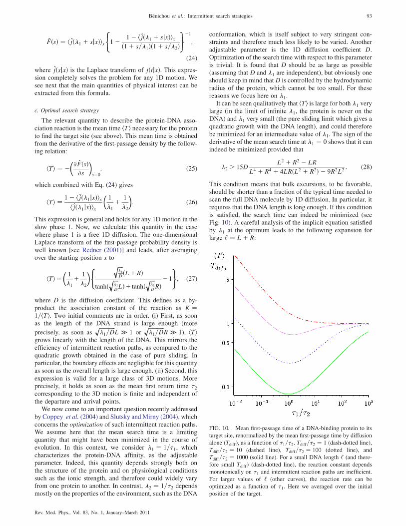
This condition means that bulk excursions, to be favorable,should be shorter than a fraction of the typical time needed toscan the full DNA molecule by 1D diffusion. In particular, itrequires that the DNA length is long enough. If this conditionis satisfied, the search time can indeed be minimized (seeFig. 10). A careful analysis of the implicit equation satisfiedby �1 at the optimum leads to the following expansion forlarge ‘ ¼ Lþ R:

FIG. 10. Mean first-passage time of a DNA-binding protein to its

target site, renormalized by the mean first-passage time by diffusion

alone (Tdiff), as a function of �1=�2. Tdiff=�2 ¼ 1 (dash-dotted line),

Tdiff=�2 ¼ 10 (dashed line), Tdiff=�2 ¼ 100 (dotted line), and

Tdiff=�2 ¼ 1000 (solid line). For a small DNA length ‘ (and there-

fore small Tdiff) (dash-dotted line), the reaction constant depends

monotonically on �1 and intermittent reaction paths are inefficient.

For larger values of ‘ (other curves), the reaction rate can be

optimized as a function of �1. Here we averaged over the initial

position of the target.



�1 ¼ �2 � 4

ffiffiffiffiffiffiffiffiffiD�2

p‘

� 8D

‘2� 40D3=2ffiffiffiffiffiffi

�2

p‘3

þO

�1

‘4

�: (29)

Equations (28) and (29) refine the result of Slutsky and Mirny(2004), which predicts that the optimal strategy is realizedwhen �1 ¼ �2. This result actually holds in the large-‘ limit,

or more precisely forffiffiffiffiffiffiffiffiffiffiffiffi�1=D

p‘ � 1. For intermediate values

of ‘, boundary effects become important and the minimumcan be significantly different.

The hTi value at the minimum is particularly interesting.We compare it to the case of pure sliding where hTsi ¼‘2=3D:

hTihTsi ¼

6

‘

ffiffiffiffiffiffiD

�1

s: (30)

The efficiency of the 3D mediated strategy is therefore muchmore important when the DNA chain is long. For example,using standard values for �1 (a few 10�2 s) and D (typically10�2 �m2=s) and for a DNA substrate of length 106 basepairs (bp), the mean reaction time is three orders of magni-tude smaller than for a pure sliding strategy. Beyond theimportance of such results for understanding the kinetics ofgene transcription, this first minimal model shows that inter-mittent reactive paths are indeed very efficient, and that theycan even allow optimization of the reaction kinetics.

3. Toward a more realistic modeling

The model introduced above provides a simple way todiscuss the minimization of the search time. Further ap-proaches have been developed to model target search byproteins. We present below the main models used in theliterature and discuss their relevance to real target searchproblems by proteins in cellular conditions.

a. Main approaches

Generally speaking, theoretical models of facilitated dif-fusion rely on the basic assumption that the protein alternatesphases of 1D diffusion along the DNA and phases of freediffusion when the protein is desorbed from the DNA. Theexistence of two such distinct states, whose dynamics isusually characterized by association-dissociation rates, issupported by direct experimental observations as discussedabove. Additionally, molecular dynamics simulations takinginto account the electrostatic interaction between the nega-tively charged DNA and the locally positively charged protein[see, for example, Dahirel et al. (2009) and Florescu andJoyeux (2009)] have shown that these two states naturallyarise on the basis of the electrostatic interaction only, sug-gesting the robustness of the facilitated diffusion mechanism.Such studies at the molecular scale could serve as a tool tocalculate the association-dissociation rates used in the modelsof facilitated diffusion discussed in this section, which alltake into account effectively only the molecular interactions.

i. Stochastic modeling. The minimal model presented inSec. III.A.2 relies on the statistical analysis of the trajectoryof a single protein and can henceforth be qualified as astochastic model. Similar stochastic methods have beenused and complemented in Lomholt et al. (2005), Eliazaret al. (2007), Lomholt et al. (2007), Eliazar et al. (2008),

Benichou et al. (2009), Lomholt et al. (2009), and Merozet al. (2009)), and have the advantage, when solvable, ofgiving access to the full distribution of the search time,yielding refined information on the search kinetics.Moreover, they can be adapted in some cases to take intoaccount anomalous transport in both the 1D and 3D phases, asdiscussed below.

ii. Kinetic approach. The main alternative to the stochas-tic approach is given by what can be called kinetic models,which assume a steady-state homogeneous concentrationof proteins, in contrast with the single-protein descriptionof stochastic models. Such models therefore rely on a mean-field approximation, which proves to be efficient evaluatingthe mean search time thanks to scaling arguments. A firstexample is given by Halford and Marko (2004), where scalingarguments are used to roughly estimate the time for theprotein to find the DNA coil, and then the time to find thetarget inside the coil, which eventually yields an optimalsliding length. More generally, the key ingredient of kineticmodels, developed mainly by Hu and Shklovskii (2006),Hu et al. (2006), and Hu et al. (2008), is that the systemis assumed to be in a stationary state. Under this hypothesis,the flux of particles delivered by the 3D diffusion into thesphere of influence of the target, whose size is defined as the‘‘antenna length’’ a, must be equal to the flux of particlesdelivered by 1D diffusion into the target. Such a balanceequation generically reads

J �D3cfreea �D1cads=�a; (31)

where the concentrations of free (cfree) and adsorbed (cads)proteins are assumed to be at equilibrium, i.e., satisfyingcfree=cads ¼ K with K the equilibrium constant associatedwith the association-dissociation rates. It is important thatthe antenna length, defined as the typical scale below whichthe dominant transport is sliding instead of 3D diffusion, hassize a when measured in 3D space, but takes another value�a when measured along the DNA. Making assumptions onthe DNA conformation (for instance, random coil or fractalglobule), different scaling laws between �a and a can beproposed. Equation (31) then permits one to determine a andhenceforth to give the scaling of the mean search time 1=J.The advantage of this method is that it permits, throughthe relation between �a and a, various models of DNAconformation to be taken into account, which is much harderto achieve in the stochastic approach. Such models, whoseresults are compatible with the stochastic approach, providein addition a useful picture of facilitated diffusion. Indeed, inthese models the effect of sliding can be seen as effectivelymaking the target of the size of the antenna length, which ismuch larger than the real target size, and therefore speedingup the search.

Finally, these two approaches are quite complementary andboth require as an input the modeling of 1D and 3D phases.The minimal model of Sec. III.A.2 describes the 1D phase asregular diffusion, while 3D phases are assumed to result incompletely random relocations over the DNA. Beyond thisminimal model, the specific description of these two phaseshas motivated numerous works and many refinements havebeen discussed in the literature. We review in the next



sections the main models that have been proposed to providea more realistic description of 1D and 3D phases.

b. Descriptions of the 1D phase (sliding and recognition)

i. Anomalous diffusion in the sliding phase. As statedabove, the phase of one-dimensional nonspecific interactionof a protein with DNA, sliding, is generally described asBrownian diffusion as in the minimal model of Sec. III.A.2.If this hypothesis seems to be confirmed by in vitro experi-ments (Kabata et al., 1993; Bonnet et al., 2008), it cannotalways be the case, in particular, in vivo. A first limitation ofthis simple description appears in the case of many proteinsbinding to DNA, as is the case in vivo, which are likely tocreate traffic jams (Sokolov et al., 2005; Li et al., 2009).Such crowding effects in one dimension are known to poten-tially lead to subdiffusive behavior. Additionally, even inthe case of a single protein, it should be kept in mind thatthe DNA sequence is not homogeneous, and the disorderin the sequence can also impact sliding. The heterogeneityin the sequence is often modeled by a disordered energylandscape, whose distribution is Gaussian (Barbi et al.,2004; Hu and Shklovskii, 2006; Wunderlich and Mirny,2008). Barbi et al. (2004) showed that in this case slidingis not purely diffusive: At short times, the protein will betrapped in local minima, leading to subdiffusive behavior.The diffusive behavior is recovered only at larger times, orequivalently for sliding lengths longer than 100 bp.

Anomalous diffusion in the sliding phase has been dis-cussed theoretically by Eliazar et al. (2007) [see also Eliazaret al. (2008) and Meroz et al. (2009)], who extended theminimal model of facilitated diffusion (Coppey et al., 2004)summarized in Sec. III.A.2. In particular, the Laplace-transformed search time distribution is obtained for severalnon-Brownian sliding motions such as ballistic, self-similar,or halted motions (in particular, when halt durations arewidely distributed, leading to subdiffusive behavior), there-fore covering standard models of anomalous diffusion. It isimportant that Eliazar et al. (2007) found that, whatever the

model of sliding, there are always regimes in which inter-mittence is favorable, similarly to the case of Browniansliding. They further showed that in the case of 3D excursionswith finite mean durations, the mean search time with anarbitrary sliding mechanism remains of order proportionalto ‘. This indicates that for long enough DNA, intermittenceis favorable for a wide range of sliding motions, either normalor anomalous, which supports the robustness of the facilitateddiffusion mechanism.

ii. Target recognition. A simplification that is often usedin the literature consists in assuming that the target is per-fectly reactive, i.e., that reaction occurs with probability 1 atthe very first passage of the protein to the target sequence.Slutsky and Mirny (2004), however, stressed that if there is anactivation barrier at the target site, the protein has a chance topass the target without entering the recognition process, andtherefore to miss it. The roughness of the energy landscapeof the sequence can then play a crucial role. If is of order1kBT, Slutsky and Mirny (2004) found that the sliding diffu-sion is fast, but that the protein has a high chance to miss thetarget. On the contrary, if is of order 5kBT, the recognitionprobability is high, but the sliding diffusion coefficient is verylow, leading to a long search time. Such a result seems to setconflicting constraints on the search, since an efficient targetsearch process requires both speed and reliability in targetrecognition. To overcome this paradox, Slutsky and Mirny(2004) proposed on the basis of direct structural observations(Kalodimos et al., 2004) that the protein can perform con-formational changes in the sliding phase, and switches be-tween a fast search state (with low ) and a slow recognitionstate (with high ) (see Fig. 11). They showed that if thetwo energy landscapes are strongly correlated, it is possibleto reconcile high speed and efficient recognition. Similarmodels of two-state proteins in the sliding phase have beenstudied more quantitatively in the frameworks of both thekinetic [see Hu et al. (2008)] and the stochastic approaches[see Benichou et al. (2009)], confirming that such a mecha-nism indeed permits a fast search with reliable recognition.

c. Descriptions of the 3D phase (jumping or hopping)

We now review the different descriptions of the 3D phase(see Fig. 12). Most of the facilitated diffusion models im-plicitly require the knowledge of the probability �ðxjx0Þ thata protein which desorbs the DNA at position x0 will even-tually rebind for the first time to the DNA at position x, wherethe coordinate x measures the distance along the chain. Thisquantity depends both on the dynamics of the protein and onthe conformation of the DNA, and in practice can be deter-mined explicitly only in the case of an ideal infinite cylindri-cal DNA (see below), which makes assumptions necessaryin realistic situations. Depending on the relocation lengthjx� x0j, 3D excursions have been given different names inthe literature, mainly either hops (referring to ‘‘small’’ jx�x0j) and jumps (referring to ‘‘large’’ jx� x0j). Since thedefinitions of jumps and hops may vary according to authors,the limit between both being somewhat arbitrary, we givebelow the one that will be used in this review.

i. Jumps. We define as jumps the 3D excursions whosestarting and ending points on the DNA sequence are uncorre-lated, i.e., such that the relocation probability �ðxjx0Þ is

FIG. 11. Sliding is often represented by diffusion with perfect

reactivity on the target. The two main directions shown for a more

realistic description of the 1D phase: On the one hand, the sliding is

not necessarily diffusive, and on the other hand, the 1D phase could

be, in fact, a combination of two phases, one fast, but with low

recognition, and another slow (or immobile), but with high recog-

nition of the target.



independent of x. This definition, of course, depends on the

DNA conformation and makes sense only for dense enough

conformations such as a random coil (for instance, for free

DNA in solution) or even denser packings that can be ex-

pected in vivo [such as fractal globule structures (Grosberg

et al., 1988)]. In such structures, sequences that are far apart

along the DNA chain can be actually very close in the 3D

space. Hence, 3D excursions whose relocation length is larger

than the typical distance between DNA segments are likely to

end at any remote location on the DNA sequence, and should

therefore be considered as jumps according to our definition.

The lower bound of the relocation length of jumps therefore

strongly depends on the DNA conformation and is in practice

hard to evaluate. In the case of interest of a confined DNA (as

in cellular conditions), the typical distance between DNA

segments can be estimated by the DNA density-density cor-

relation length c. This suggests an alternative and equivalent

definition of jumps as 3D excursions whose relocation length

is larger than c. Awidespread assumption used, for example,

in the minimal model of Sec. III.A.2 [see also Hu et al.

(2006) at scales larger then the antenna size or Coppey et al.

(2004), Eliazar et al. (2007), and Benichou et al. (2009)]

consists in taking all 3D excursions as jumps, i.e., as random

uniform relocations over the DNA. Even if not exact, this

assumption has been checked numerically on the example of

a quenched self-avoiding DNA and has proved to be very

satisfactory (Sheinman and Kafri, 2009) at high enough DNA

concentration. Interestingly, this definition of jumps high-

lights the importance of the effect of the local DNA concen-

tration on the search efficiency, as observed in van den Broek

et al. (2008); Lomholt et al. (2009): the more densely packed

the DNA, the smaller the correlation length c, and therefore

the higher the probability of jumps enabling the protein to

explore previously unscanned areas, and the less the time

spent in 3D phases.The assumption that all excursions of relocation length

larger than the typical distance between DNA segments lead

to a completely uniform relocation over the DNA is, however,

not exact. Indeed, large-scale correlations in the 3D confor-

mation of the DNA chain may exist, as in the model case of a

free random coil conformation. In particular, in eukaryotes,

where DNA is packed in the nucleus, recent studies such as

that of Lieberman-Aiden et al. (2009) support a hierarchical

structure of DNA that could induce long-range correlations in

the conformation and therefore a nonuniform relocation

probability. The impact of DNA conformation on the reloca-

tion probability has been tested on the example of an an-

nealed wormlike chain polymer by Dıaz de la Rosa et al.

(2010) who found that at short times, three-dimensional

excursions of approximately the DNA persistence length

are actually less abundant than both shorter and slightly larger

relocations: by definition, closer sequences along the DNA

are closer in 3D space, but sequences farther than the persis-

tence length can take advantage of loops and actually be even

closer in 3D space. More generally, the loop statistics impacts

on the relocation probability and can lead to a nonuniform

relocation probability �ðxjx0Þ. Lomholt et al. (2005) argued

that since polymers form loops whose linear size x is distrib-

uted according to pðxÞ � jxj�1�� (for instance, � ¼ 0:5 for

Gaussian chains; � ’ 1:2 for self-avoiding walks), reloca-

tions distributed according to the same law are favored and

should also be taken into account. In an annealed version of

such a model, they showed that depending on � the optimal

strategy can vary widely. It should be added that loops can

enable another relocation mechanism for proteins with mul-

tiple binding sites called intersegmental transfer [see Hu and

Shklovskii (2007) and Sheinman and Kafri (2009)], which

can be shown for modeling purposes to be widely equivalent

to 3D excursions. Finally, the approximation of uniform

random relocations has proved to be useful and can be

validated numerically for simple DNA conformations

(Sheinman and Kafri, 2009), but a better knowledge of the

in vivo conformation of DNA would be necessary to assess

more precisely the relocation probability.ii. Hops. Echoing the definition of jumps, we define hops

as 3D excursions whose starting and ending points on the

DNA sequence are correlated, or equivalently as 3D excur-

sions whose relocation length is smaller than the typical

distance between DNA segments, which is given by the

correlation length c for confined DNA. Because of their

local character, hops are often effectively taken into account

in the sliding mechanism [see, for example, Hu et al. (2006)].

Although this assumption is useful in practice, it also raises

additional questions. (i) First, hops do not continuously ex-

plore the DNA, and a protein performing hops have higher

chances to miss the target (note that hops permit as a counter-

part the bypassing of obstacles on the DNA), and this non-

perfect reactivity has to be taken into account. (ii) Second,

if hops are included in an effective sliding mechanism,

then the effective diffusion coefficient has to be determined,

as well as the effective transition rate from this effective

sliding state to the jumping state. This last point amounts in

practice in calculating the relocation probability �ðxjx0Þ ofhops, which gives as a by-product the probability that after

desorption from DNA the protein performs a jump rather

than a hop.This problem, which has been studied numerically by

Wunderlich and Mirny (2008), can actually be studied

Hop

Jump

Loop effect

FIG. 12. Description of 3D excursions. Jumps are 3D excursions

whose starting and ending points on the DNA sequence are un-

correlated. In practice, for confined DNA conformations as in a

cellular medium, jumps have a span (measured along the DNA

contour) larger than the density-density correlation length c of

DNA. Conversely, hops are 3D excursions whose starting and

ending points on the DNA sequence are correlated, or equivalently

3D excursions whose relocation length is smaller than the correla-

tion length c.



analytically (Loverdo et al., 2009), since at the scale of hops,which are smaller than the DNA persistence length p, the

DNA can be simply modeled as a cylinder of effective radiusa ¼ RDNA þ Rprotein (see Fig. 13, left). Denoting by D the 3D

diffusion coefficient of the protein (assumed pointlike), thedensity probability �ðxjr0Þ of being adsorbed on the DNA atthe longitudinal abscissa x, starting from the point r0, thensatisfies [for further details on derivation, see Berg andBlomberg (1976), Levitz et al. (2008), Loverdo et al.(2009), Chechkin et al. (2009), and Benichou et al. (2010,2011) for similar analyses]:

�r0�ðxjr0Þ ¼ 0: (32)

Assuming a radiative boundary condition on the cylindersurface to account for the adsorption rate on DNA,

@r0�ðxjr0Þðr0 ¼ aÞ ¼ ��ðxjr0Þðr0 ¼ aÞ; (33)

one can show that

�ðxjr0Þ ¼ 1

�

Z 1

0cosðkxÞ K0ðkr0Þ

K0ðkaÞ þK1ðkaÞk=�dk; (34)

where Ki are Bessel functions. This relocation distribution, ingood agreement with experimental data from Bonnet et al.(2008) obtained on an extended DNA molecule, enables oneto address the questions of point (ii) above. First, Eq. (34)gives the analytical distribution of hops, since for x < c theDNA can be well approximated by a cylinder. In turn, asshown by Loverdo et al. (2009), this gives access to theeffective diffusion coefficient of a combined motion of slid-ing and hops. Second, according to our definition, all reloca-tions with x > c will be jumps. Thus, the probability that a3D relocation is a jump rather than a hop is given by thecomplementary cumulative distribution

Cðx¼cÞ¼Zjxj>c

�ðxjr0Þdx� lnðr0=aÞþ1=�a

lnðc=aÞ : (35)

Returning to the search problem, in regimes where jumpsare favorable, decreasing the correlation length speeds up thesearch process, as found by van den Broek et al. (2008).

iii. Crowding effects. In both prokaryotes and eukaryotes,the cellular medium is very crowded, and 3D excursions of

proteins are likely to be hindered. The normal or anomalous

nature of transport in cellular medium is still debated. Forinstance, Dix and Verkman (2008) supported the idea that 3D

motion is mostly normal diffusion, whereas Malchus and

Weiss (2010) suggested that there is more and more evidencefor subdiffusion. Experimentally, it is found that some tracers

exhibit transient behavior (subdiffusive at small time scales,diffusive at larger time scales): Measures, however, depend

on the size and nature of the tracer, on the time and length

scales covered, and on other experimental conditions, whichmay explain the lack of consensus on the problem. The

influence of subdiffusion on the target search will depend

on the microscopic mechanism at play. There are threemain mechanisms leading to subdiffusion, as outlined in

Appendix A: random walk on a fractal medium, randomwalk with long waiting times (CTRW) [continuous-time

random walks], or random walk with long-range correlations

such as fractional Brownian motion (FBM). Which of thesepossibilities best describes transport in crowded environ-

ments such as the cellular medium is, however, still unclear

[see He et al. (2008), Bancaud et al. (2009), Szymanski andWeiss (2009), or Tejedor et al. (2010) for various opinions on

the subject].Lomholt et al. (2007) explored the effect of a crowded

environment with subdiffusion hr2ðtÞi / t� (0<�< 1)caused by waiting times distributed as pðtÞ � ��=t1þ�.

They argued that because of these waiting times, the proba-bility that the protein has not yet left the DNA at time t andthe probability that an unbound protein has not yet bound to

DNA after a time t both scale as 1=t1þ�. Their results havetwo main practical implications. On the one hand, in an

experiment, since proteins can remain stuck for very longtimes, ensemble averages do not lead to the same results as

time averages as was also highlighted by He et al. (2008). On

the other hand, since proteins would slide for a longer timeand since it would take them a very long time to return to

the DNA, the genes’ coding for transcription factors should

be close to their target sequences, as also outlined byWunderlich and Mirny (2008). Analytical determination of

the relocation distribution above can be extended to a fractalmedium (Loverdo et al., 2009). In this case, using the

O’Shaughnessy and Procaccia (1985) formalism, the

large-x behavior of the relocation distribution is obtained as

�ðxjr0Þ � rdw�d?

f

0 =x1þdw�d?f , where dkf is the dimension of the

projection of the fractal on the axis parallel to the cylinder

(Loverdo et al., 2009). Hence, the relocation distributionalways decays faster than in the case of normal diffusion

�1=ðzln2ðz=aÞÞ. As a consequence, the proportion of jumps

in the case of random conformation of DNA in the fractal

type crowding scales as CðÞ � �dwþd?f : it is much smaller

than for regular diffusion, which shows that fractal crowding

favors hops and changes the overall intermittent search.

d. Beyond the mean: Variability of the search time

Minimizing the mean search time is the optimizationprocedure most often used [see, for example, Coppey et al.

(2004)]. However, the entire distribution of the search time is

needed to assess the search kinetics on all time scales. In thecase of simple exponential distributions of the search time,

FIG. 13. Facilitated diffusion of a protein on DNA. Left:

Schematic definition of sliding, hopping, and jumping. Hops are

3D excursions whose starting and ending points on the DNA

sequence are correlated, or equivalently 3D excursions whose

relocation length is smaller than the typical distance between

DNA segments. In the case of confined DNA, this distance is

estimated by the DNA density-density correlation length c.

Right: Model parameters.



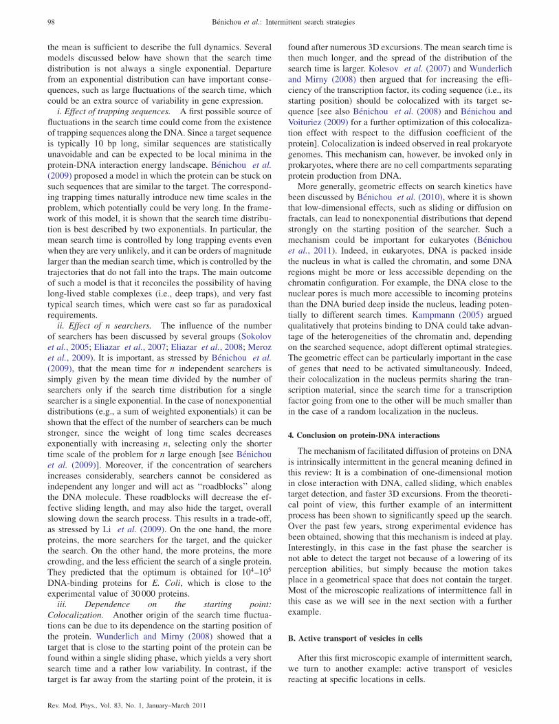
the mean is sufficient to describe the full dynamics. Several

models discussed below have shown that the search time

distribution is not always a single exponential. Departure

from an exponential distribution can have important conse-

quences, such as large fluctuations of the search time, which

could be an extra source of variability in gene expression.i. Effect of trapping sequences. A first possible source of

fluctuations in the search time could come from the existence

of trapping sequences along the DNA. Since a target sequence

is typically 10 bp long, similar sequences are statistically

unavoidable and can be expected to be local minima in the

protein-DNA interaction energy landscape. Benichou et al.

(2009) proposed a model in which the protein can be stuck on

such sequences that are similar to the target. The correspond-

ing trapping times naturally introduce new time scales in the

problem, which potentially could be very long. In the frame-

work of this model, it is shown that the search time distribu-

tion is best described by two exponentials. In particular, the

mean search time is controlled by long trapping events even

when they are very unlikely, and it can be orders of magnitude

larger than the median search time, which is controlled by the

trajectories that do not fall into the traps. The main outcome

of such a model is that it reconciles the possibility of having

long-lived stable complexes (i.e., deep traps), and very fast

typical search times, which were cast so far as paradoxical

requirements.ii. Effect of n searchers. The influence of the number

of searchers has been discussed by several groups (Sokolov

et al., 2005; Eliazar et al., 2007; Eliazar et al., 2008; Meroz

et al., 2009). It is important, as stressed by Benichou et al.

(2009), that the mean time for n independent searchers is

simply given by the mean time divided by the number of

searchers only if the search time distribution for a single

searcher is a single exponential. In the case of nonexponential

distributions (e.g., a sum of weighted exponentials) it can be

shown that the effect of the number of searchers can be much

stronger, since the weight of long time scales decreases

exponentially with increasing n, selecting only the shorter

time scale of the problem for n large enough [see Benichou

et al. (2009)]. Moreover, if the concentration of searchers

increases considerably, searchers cannot be considered as

independent any longer and will act as ‘‘roadblocks’’ along

the DNA molecule. These roadblocks will decrease the ef-

fective sliding length, and may also hide the target, overall

slowing down the search process. This results in a trade-off,

as stressed by Li et al. (2009). On the one hand, the more

proteins, the more searchers for the target, and the quicker

the search. On the other hand, the more proteins, the more

crowding, and the less efficient the search of a single protein.

They predicted that the optimum is obtained for 104–105

DNA-binding proteins for E. Coli, which is close to the

experimental value of 30 000 proteins.iii. Dependence on the starting point:

Colocalization. Another origin of the search time fluctua-

tions can be due to its dependence on the starting position of

the protein. Wunderlich and Mirny (2008) showed that a

target that is close to the starting point of the protein can be

found within a single sliding phase, which yields a very short

search time and a rather low variability. In contrast, if the

target is far away from the starting point of the protein, it is

found after numerous 3D excursions. The mean search time is

then much longer, and the spread of the distribution of the

search time is larger. Kolesov et al. (2007) and Wunderlich

and Mirny (2008) then argued that for increasing the effi-

ciency of the transcription factor, its coding sequence (i.e., its

starting position) should be colocalized with its target se-

quence [see also Benichou et al. (2008) and Benichou and

Voituriez (2009) for a further optimization of this colocaliza-

tion effect with respect to the diffusion coefficient of the

protein]. Colocalization is indeed observed in real prokaryote

genomes. This mechanism can, however, be invoked only in

prokaryotes, where there are no cell compartments separating

protein production from DNA.More generally, geometric effects on search kinetics have

been discussed by Benichou et al. (2010), where it is shown

that low-dimensional effects, such as sliding or diffusion on

fractals, can lead to nonexponential distributions that depend

strongly on the starting position of the searcher. Such a

mechanism could be important for eukaryotes (Benichou

et al., 2011). Indeed, in eukaryotes, DNA is packed inside

the nucleus in what is called the chromatin, and some DNA

regions might be more or less accessible depending on the

chromatin configuration. For example, the DNA close to the

nuclear pores is much more accessible to incoming proteins

than the DNA buried deep inside the nucleus, leading poten-

tially to different search times. Kampmann (2005) argued

qualitatively that proteins binding to DNA could take advan-

tage of the heterogeneities of the chromatin and, depending

on the searched sequence, adopt different optimal strategies.

The geometric effect can be particularly important in the case

of genes that need to be activated simultaneously. Indeed,

their colocalization in the nucleus permits sharing the tran-

scription material, since the search time for a transcription

factor going from one to the other will be much smaller than

in the case of a random localization in the nucleus.

4. Conclusion on protein-DNA interactions

The mechanism of facilitated diffusion of proteins on DNA

is intrinsically intermittent in the general meaning defined in

this review: It is a combination of one-dimensional motion

in close interaction with DNA, called sliding, which enables

target detection, and faster 3D excursions. From the theoreti-

cal point of view, this further example of an intermittent

process has been shown to significantly speed up the search.

Over the past few years, strong experimental evidence has

been obtained, showing that this mechanism is indeed at play.

Interestingly, in this case in the fast phase the searcher is

not able to detect the target not because of a lowering of its

perception abilities, but simply because the motion takes

place in a geometrical space that does not contain the target.

Most of the microscopic realizations of intermittence fall in

this case as we will see in the next section with a further

example.

B. Active transport of vesicles in cells

After this first microscopic example of intermittent search,

we turn to another example: active transport of vesicles

reacting at specific locations in cells.



1. Active transport in cells

Various motor proteins such as kinesins or myosins areable to convert the chemical fuel provided by adenosinetriphosphate (ATP) into mechanical work by interactingwith the semiflexible oriented filaments (mainly F-actin andmicrotubules) of the cytoskeleton (Alberts, 2002). Becausemany molecules or larger cellular organelles such as vesicles,lysosomes, or mitochondria (hereafter referred to as tracerparticles) can randomly bind and unbind to motors, the over-all transport of a tracer in the cell can be described asalternating phases of standard diffusive transport (sometimessubdiffusive), and phases of active directed transport poweredby motor proteins (Alberts, 2002; Salman et al., 2005), seeFig. 14. In particular, Huet et al. (2006) studied the rate oftransitions between ballistic, diffusive, and ‘‘on the target’’states of vesicles, and found that the vesicles studied are muchmore likely to react in the free diffusive phase than whenbound to motors. Active transport in this case is thereforeclearly a further example of intermittent behavior. Activetransport in cells has been extensively studied both experi-mentally, for instance, by single particle tracking methods(Sheetz and Spudich, 1983; Howard et al., 1989; Caspi et al.,2000; Caspi et al., 2002), and theoretically by evaluating themean displacement of a tracer (Shlesinger and Klafter, 1989;Ajdari, 1995; Salman et al., 2005), or stationary concentra-tion profiles (Nedelec et al., 2001). This transport is impor-tant, for example, for dynamically regulating the distributionof proteins such as membrane receptors.

Most cell functions are regulated by coordinated chemicalreactions that involve low concentrations of reactants (such asribosomes or vesicles carrying targeted proteins), and that aretherefore limited by transport. An analytical model based onthe idea of intermittence has been introduced by Loverdoet al. (2008) [see also Mirny (2008) and Loverdo et al.(2009a)], enables the determination of the kinetic constantof transport limited reactions in active media, and furthershows that the kinetic constant can be optimized. We givebelow the main results of the model; further details can befound in Appendix B.

2. Model

The model relies on the idea of intermittent search strat-egies and has important similarities with the models of

Sec. II, which are discussed in Sec. IV. We consider a tracerparticle evolving in a d-dimensional space (in practice d ¼1; 2; 3), which performs thermal diffusion motions of diffu-sion coefficient D (denoted phases 1), randomly interruptedby ballistic excursions bound to motors (referred to asphases 2) of constant velocity V and direction pointing inthe solid angle !V (see Fig. 15). The distribution of thefilaments’ orientation is denoted by �ð!VÞ and will be takenas either disordered or polarized (see Figs. 15, 17, and 19),which schematically reproduces the different states of thecytoskeleton (Alberts, 2002). The random duration of eachphase i is assumed to be exponentially distributed with mean�i. The tracer T can react with reactants R (supposed immo-bile) during free diffusion phases 1 only, as T is assumed to beinactive when bound to motors. Reaction occurs with a finiteprobability per unit of time k when the tracer-reactant dis-tance is smaller than a given reaction radius a. In whatfollows the kinetic constant K of the reaction T þ R ! R isexplicitly determined.

3. Methods

We now present the basic equations in the case of areactant centered in a spherical domain of radius b withreflecting boundary. This geometry both mimics therelevant situation of a single target and provides a mean-field

FIG. 14. Transport options for vesicles inside cells.

FIG. 15. Vesicle transport in the bulk (three dimensions).



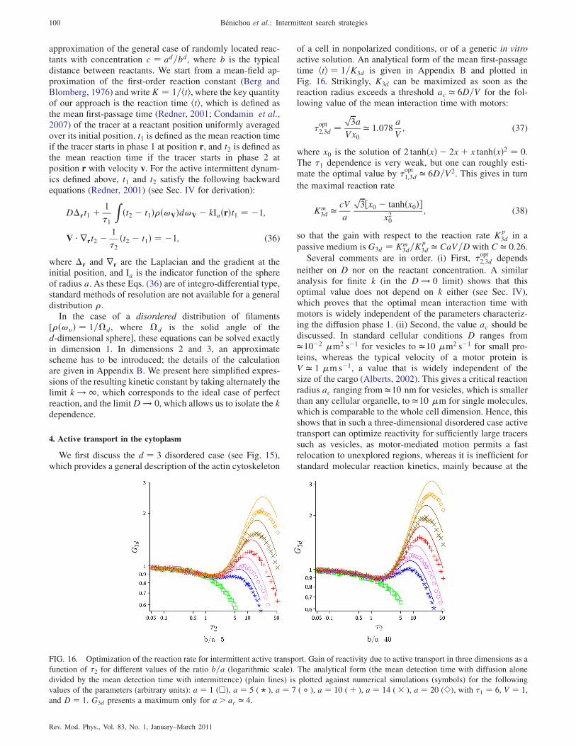
approximation of the general case of randomly located reac-tants with concentration c ¼ ad=bd, where b is the typicaldistance between reactants. We start from a mean-field ap-proximation of the first-order reaction constant (Berg andBlomberg, 1976) and writeK ¼ 1=hti, where the key quantityof our approach is the reaction time hti, which is defined asthe mean first-passage time (Redner, 2001; Condamin et al.,2007) of the tracer at a reactant position uniformly averagedover its initial position. t1 is defined as the mean reaction timeif the tracer starts in phase 1 at position r, and t2 is defined asthe mean reaction time if the tracer starts in phase 2 atposition r with velocity v. For the active intermittent dynam-ics defined above, t1 and t2 satisfy the following backwardequations (Redner, 2001) (see Sec. IV for derivation):

D�rt1 þ 1

�1

Zðt2 � t1Þ�ð!VÞd!V � kIaðrÞt1 ¼ �1;

V � rrt2 � 1

�2ðt2 � t1Þ ¼ �1; (36)

where �r and rr are the Laplacian and the gradient at theinitial position, and Ia is the indicator function of the sphereof radius a. As these Eqs. (36) are of integro-differential type,standard methods of resolution are not available for a generaldistribution �.

In the case of a disordered distribution of filaments[�ð!vÞ ¼ 1=�d, where �d is the solid angle of thed-dimensional sphere], these equations can be solved exactlyin dimension 1. In dimensions 2 and 3, an approximatescheme has to be introduced; the details of the calculationare given in Appendix B. We present here simplified expres-sions of the resulting kinetic constant by taking alternately thelimit k ! 1, which corresponds to the ideal case of perfectreaction, and the limitD ! 0, which allows us to isolate the kdependence.

4. Active transport in the cytoplasm

We first discuss the d ¼ 3 disordered case (see Fig. 15),which provides a general description of the actin cytoskeleton

of a cell in nonpolarized conditions, or of a generic in vitroactive solution. An analytical form of the mean first-passagetime hti ¼ 1=K3d is given in Appendix B and plotted inFig. 16. Strikingly, K3d can be maximized as soon as thereaction radius exceeds a threshold ac ’ 6D=V for the fol-lowing value of the mean interaction time with motors:

�opt2;3d ¼

ffiffiffi3

pa

Vx0’ 1:078

a

V; (37)

where x0 is the solution of 2 tanhðxÞ � 2xþ x tanhðxÞ2 ¼ 0.The �1 dependence is very weak, but one can roughly esti-mate the optimal value by �

opt1;3d ’ 6D=V2. This gives in turn

the maximal reaction rate

Km3d ’ cV

a

ffiffiffi3

p ½x0 � tanhðx0Þ�x20

; (38)

so that the gain with respect to the reaction rate Kp3d in a

passive medium is G3d ¼ Km3d=K

p3d ’ CaV=D with C ’ 0:26.

Several comments are in order. (i) First, �opt2;3d depends

neither on D nor on the reactant concentration. A similaranalysis for finite k (in the D ! 0 limit) shows that thisoptimal value does not depend on k either (see Sec. IV),which proves that the optimal mean interaction time withmotors is widely independent of the parameters characteriz-ing the diffusion phase 1. (ii) Second, the value ac should bediscussed. In standard cellular conditions D ranges from’10�2 �m2 s�1 for vesicles to ’10 �m2 s�1 for small pro-teins, whereas the typical velocity of a motor protein isV ’ 1 �ms�1, a value that is widely independent of thesize of the cargo (Alberts, 2002). This gives a critical reactionradius ac ranging from ’10 nm for vesicles, which is smallerthan any cellular organelle, to ’10 �m for single molecules,which is comparable to the whole cell dimension. Hence, thisshows that in such a three-dimensional disordered case activetransport can optimize reactivity for sufficiently large tracerssuch as vesicles, as motor-mediated motion permits a fastrelocation to unexplored regions, whereas it is inefficient forstandard molecular reaction kinetics, mainly because at the

FIG. 16. Optimization of the reaction rate for intermittent active transport. Gain of reactivity due to active transport in three dimensions as a

function of �2 for different values of the ratio b=a (logarithmic scale). The analytical form (the mean detection time with diffusion alone

divided by the mean detection time with intermittence) (plain lines) is plotted against numerical simulations (symbols) for the following

values of the parameters (arbitrary units): a ¼ 1 (h), a ¼ 5 ( ? ), a ¼ 7 ( � ), a ¼ 10 (þ ), a ¼ 14 ( ), a ¼ 20 (�), with �1 ¼ 6, V ¼ 1,and D ¼ 1. G3d presents a maximum only for a > ac ’ 4.



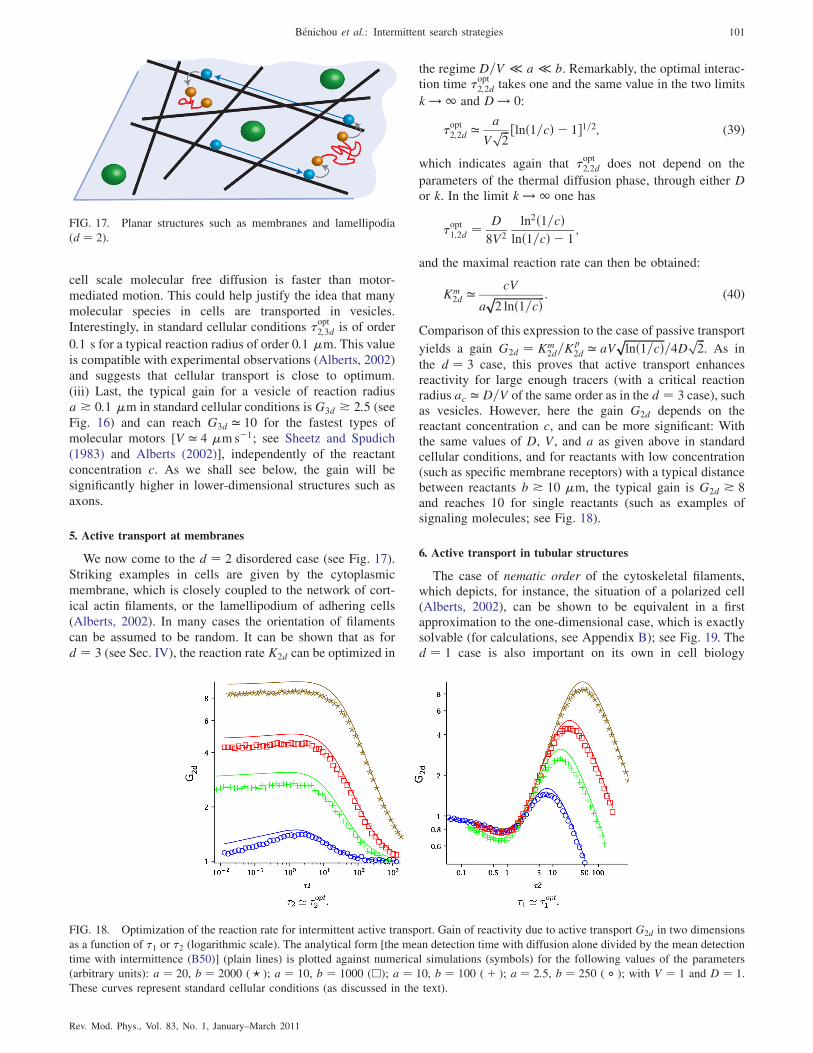
cell scale molecular free diffusion is faster than motor-

mediated motion. This could help justify the idea that many

molecular species in cells are transported in vesicles.

Interestingly, in standard cellular conditions �opt2;3d is of order

0:1 s for a typical reaction radius of order 0:1 �m. This value

is compatible with experimental observations (Alberts, 2002)

and suggests that cellular transport is close to optimum.

(iii) Last, the typical gain for a vesicle of reaction radius

a * 0:1 �m in standard cellular conditions is G3d * 2:5 (seeFig. 16) and can reach G3d ’ 10 for the fastest types of

molecular motors [V ’ 4 �ms�1; see Sheetz and Spudich

(1983) and Alberts (2002)], independently of the reactant

concentration c. As we shall see below, the gain will be

significantly higher in lower-dimensional structures such as

axons.

5. Active transport at membranes

We now come to the d ¼ 2 disordered case (see Fig. 17).

Striking examples in cells are given by the cytoplasmic

membrane, which is closely coupled to the network of cort-

ical actin filaments, or the lamellipodium of adhering cells

(Alberts, 2002). In many cases the orientation of filaments

can be assumed to be random. It can be shown that as for

d ¼ 3 (see Sec. IV), the reaction rate K2d can be optimized in

the regime D=V � a � b. Remarkably, the optimal interac-tion time �

opt2;2d takes one and the same value in the two limits

k ! 1 and D ! 0:

�opt2;2d ’

a

Vffiffiffi2

p ½lnð1=cÞ � 1�1=2; (39)

which indicates again that �opt2;2d does not depend on the

parameters of the thermal diffusion phase, through either Dor k. In the limit k ! 1 one has

�opt1;2d ¼

D

8V2

ln2ð1=cÞlnð1=cÞ � 1

;

and the maximal reaction rate can then be obtained:

Km2d ’ cV

affiffiffiffiffiffiffiffiffiffiffiffiffiffiffiffiffiffiffi2 lnð1=cÞp : (40)

Comparison of this expression to the case of passive transport

yields a gain G2d ¼ Km2d=K

p2d ’ aV

ffiffiffiffiffiffiffiffiffiffiffiffiffiffiffilnð1=cÞp

=4Dffiffiffi2

p. As in

the d ¼ 3 case, this proves that active transport enhancesreactivity for large enough tracers (with a critical reactionradius ac ’ D=V of the same order as in the d ¼ 3 case), suchas vesicles. However, here the gain G2d depends on thereactant concentration c, and can be more significant: Withthe same values of D, V, and a as given above in standardcellular conditions, and for reactants with low concentration(such as specific membrane receptors) with a typical distancebetween reactants b * 10 �m, the typical gain is G2d * 8and reaches 10 for single reactants (such as examples ofsignaling molecules; see Fig. 18).

6. Active transport in tubular structures

The case of nematic order of the cytoskeletal filaments,which depicts, for instance, the situation of a polarized cell(Alberts, 2002), can be shown to be equivalent in a firstapproximation to the one-dimensional case, which is exactlysolvable (for calculations, see Appendix B); see Fig. 19. Thed ¼ 1 case is also important on its own in cell biology

FIG. 17. Planar structures such as membranes and lamellipodia

(d ¼ 2).

FIG. 18. Optimization of the reaction rate for intermittent active transport. Gain of reactivity due to active transport G2d in two dimensions

as a function of �1 or �2 (logarithmic scale). The analytical form [the mean detection time with diffusion alone divided by the mean detection

time with intermittence (B50)] (plain lines) is plotted against numerical simulations (symbols) for the following values of the parameters

(arbitrary units): a ¼ 20, b ¼ 2000 ( ? ); a ¼ 10, b ¼ 1000 (h); a ¼ 10, b ¼ 100 (þ ); a ¼ 2:5, b ¼ 250 ( � ); with V ¼ 1 and D ¼ 1.These curves represent standard cellular conditions (as discussed in the text).



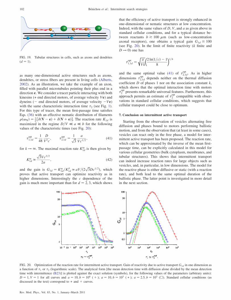
as many one-dimensional active structures such as axons,dendrites, or stress fibers are present in living cells (Alberts,2002). As an illustration, we take the example of an axon,filled with parallel microtubules pointing their plus end in adirection e. We consider a tracer particle interacting with bothkinesins (+ end directed motors, of average velocity Ve) anddyneins (� end directed motors, of average velocity �Ve)with the same characteristic interaction time �2 (see Fig. 1).For this type of tracer, the mean first-passage time satisfiesEqs. (36) with an effective nematic distribution of filaments�ð!VÞ ¼ 1

2 ½�ðV � eÞ þ �ðV þ eÞ�. The reaction rate K1d is

maximized in the regime D=V � a � b for the followingvalues of the characteristic times (see Fig. 20):

�opt1;1d ¼ 1

48

D

V2c; �

opt2;1d ¼ 1ffiffiffi

3p a

Vc1=2; (41)

for k ! 1. The maximal reaction rate Km1d is then given by

Km1d ’

ffiffiffi3

pVc3=2

2a; (42)

and the gain is G1d ¼ Km1d=K

p1d ’ aV=ð2 ffiffiffi

3p

Dc1=2Þ, which

proves that active transport can optimize reactivity as inhigher dimensions. Interestingly the c dependence of thegain is much more important than for d ¼ 2; 3, which shows

that the efficiency of active transport is strongly enhanced inone-dimensional or nematic structures at low concentration.Indeed, with the same values of D, V, and a as given above instandard cellular conditions, and for a typical distance be-tween reactants b * 100 �m (such as low-concentrationaxonal receptors), one obtains a typical gain G1d * 100(see Fig. 20). In the limit of finite reactivity (k finite andD ! 0) one has

�opt1;1d ¼

ffiffiffiffiffiffia

Vk

r �2 lnð1=cÞ � 1

8

�1=4

and the same optimal value (41) of �opt2;1d. As in higher

dimensions �opt2;1d depends neither on the thermal diffusion

coefficient D of phases 1 nor on the association constant k,which shows that the optimal interaction time with motors�opt2 presents remarkable universal features. Furthermore, this

approach permits an estimate of �opt2 compatible with obser-

vations in standard cellular conditions, which suggests thatcellular transport could be close to optimum.

7. Conclusion on intermittent active transport

Starting from the observation of vesicles alternating freediffusion and phases bound to motors performing ballisticmotion, and from the observation that (at least in some cases),vesicles can react only in the free phase, a model for inter-mittent active transport has been proposed. The reaction rate,which can be approximated by the inverse of the mean first-passage time, can be explicitly calculated in this model forvarious cellular geometries (bulk cytoplasm, membranes, andtubular structures). This shows that intermittent transportcan indeed increase reaction rates for large objects such asvesicles, and, in particular, in low dimensions. The model forthe reactive phase is either diffusive or static (with a reactionrate), and both lead to the same optimal duration of theballistic phase. The latter point is investigated in more detailin the next section.

FIG. 19. Tubular structures in cells, such as axons and dendrites

(d ¼ 1).

FIG. 20. Optimization of the reaction rate for intermittent active transport. Gain of reactivity due to active transport G1d in one dimension as

a function of �1 or �2 (logarithmic scale). The analytical form [the mean detection time with diffusion alone divided by the mean detection

time with intermittence (B23)] is plotted against the exact solution (symbols), for the following values of the parameters (arbitrary units):

D ¼ 1; V ¼ 1 for all curves and a ¼ 10; b ¼ 104 (þ ); a ¼ 10; b ¼ 103 ( � ); a ¼ 2:5; b ¼ 103 (h). Standard cellular conditions (as

discussed in the text) correspond to � and þ curves.



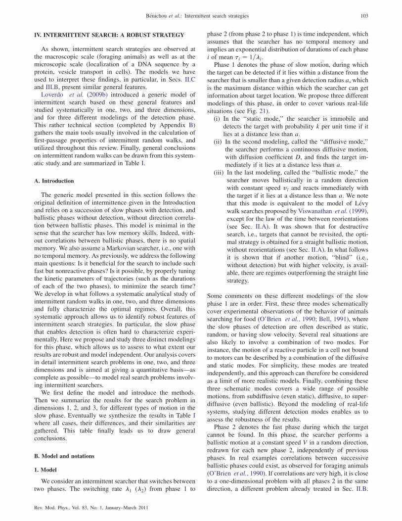
IV. INTERMITTENT SEARCH: A ROBUST STRATEGY

As shown, intermittent search strategies are observed atthe macroscopic scale (foraging animals) as well as at themicroscopic scale (localization of a DNA sequence by aprotein, vesicle transport in cells). The models we haveused to interpret these findings, in particular, in Secs. II.Cand III.B, present similar general features.

Loverdo et al. (2009b) introduced a generic model ofintermittent search based on these general features andstudied systematically in one, two, and three dimensions,and for three different modelings of the detection phase.This rather technical section (completed by Appendix B)gathers the main tools usually involved in the calculation offirst-passage properties of intermittent random walks, andutilized throughout this review. Finally, general conclusionson intermittent random walks can be drawn from this system-atic study and are summarized in Table I.

A. Introduction

The generic model presented in this section follows theoriginal definition of intermittence given in the Introductionand relies on a succession of slow phases with detection, andballistic phases without detection, without direction correla-tion between ballistic phases. This model is minimal in thesense that the searcher has low memory skills. Indeed, with-out correlations between ballistic phases, there is no spatialmemory. We also assume a Markovian searcher, i.e., one withno temporal memory. As previously, we address the followingmain questions: Is it beneficial for the search to include suchfast but nonreactive phases? Is it possible, by properly tuningthe kinetic parameters of trajectories (such as the durationsof each of the two phases), to minimize the search time?We develop in what follows a systematic analytical study ofintermittent random walks in one, two, and three dimensionsand fully characterize the optimal regimes. Overall, thissystematic approach allows us to identify robust features ofintermittent search strategies. In particular, the slow phasethat enables detection is often hard to characterize experi-mentally. Here we propose and study three distinct modelingsfor this phase, which allows us to assess to what extent ourresults are robust and model independent. Our analysis coversin detail intermittent search problems in one, two, and threedimensions and is aimed at giving a quantitative basis—ascomplete as possible—to model real search problems involv-ing intermittent searchers.

We first define the model and introduce the methods.Then we summarize the results for the search problem indimensions 1, 2, and 3, for different types of motion in theslow phase. Eventually we synthesize the results in Table Iwhere all cases, their differences, and their similarities aregathered. This table finally leads us to draw generalconclusions.

B. Model and notations

1. Model

We consider an intermittent searcher that switches betweentwo phases. The switching rate �1 (�2) from phase 1 to

phase 2 (from phase 2 to phase 1) is time independent, which

assumes that the searcher has no temporal memory and

implies an exponential distribution of durations of each phase

i of mean �i ¼ 1=�i.Phase 1 denotes the phase of slow motion, during which

the target can be detected if it lies within a distance from the

searcher that is smaller than a given detection radius a, whichis the maximum distance within which the searcher can get

information about target location. We propose three different

modelings of this phase, in order to cover various real-life

situations (see Fig. 21).(i) In the ‘‘static mode,’’ the searcher is immobile and

detects the target with probability k per unit time if it

lies at a distance less than a.(ii) In the second modeling, called the ‘‘diffusive mode,’’

the searcher performs a continuous diffusive motion,

with diffusion coefficient D, and finds the target im-

mediately if it lies at a distance less than a.(iii) In the last modeling, called the ‘‘ballistic mode,’’ the

searcher moves ballistically in a random direction

with constant speed vl and reacts immediately with

the target if it lies at a distance less than a. We note

that this mode is equivalent to the model of Levy

walk searches proposed by Viswanathan et al. (1999),

except for the law of the time between reorientations

(see Sec. II.A). It was shown that for destructive

search, i.e., targets that cannot be revisited, the opti-

mal strategy is obtained for a straight ballistic motion,

without reorientations (see Sec. II.A). In what follows

it is shown that if another motion, ‘‘blind’’ (i.e.,

without detection) but with higher velocity, is avail-

able, there are regimes outperforming the straight line

strategy.

Some comments on these different modelings of the slow

phase 1 are in order. First, these three modes schematically

cover experimental observations of the behavior of animals

searching for food (O’Brien et al., 1990; Bell, 1991), where

the slow phases of detection are often described as static,

random, or having slow velocity. Several real situations are

also likely to involve a combination of two modes. For

instance, the motion of a reactive particle in a cell not bound

to motors can be described by a combination of the diffusive

and static modes. For simplicity, these modes are treated

independently, and this approach can therefore be considered

as a limit of more realistic models. Finally, combining these

three schematic modes covers a wide range of possible

motions, from subdiffusive (even static), diffusive, to super-

diffusive (even ballistic). Beyond the modeling of real-life

systems, studying different detection modes enables us to

assess the robustness of the results.Phase 2 denotes the fast phase during which the target

cannot be found. In this phase, the searcher performs a

ballistic motion at a constant speed V in a random direction,

redrawn for each new phase 2, independently of previous

phases. In real examples correlations between successive

ballistic phases could exist, as observed for foraging animals

(O’Brien et al., 1990). If correlations are very high, it is close

to a one-dimensional problem with all phases 2 in the same

direction, a different problem already treated in Sec. II.B.



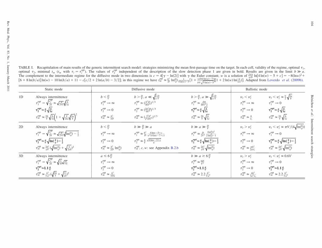
TABLE I. Recapitulation of main results of the generic intermittent search model: strategies minimizing the mean first-passage time on the target. In each cell, validity of the regime, optimal �1,optimal �2, minimal tm (tm with �i ¼ �opti ). The values of �opt2 independent of the description of the slow detection phase 1 are given in bold. Results are given in the limit b � a.The complement to the intermediate regime for the diffusive mode in two dimensions is c ¼ 4½ � lnð2Þ� with the Euler constant; w is a solution of 2Vb

wD ln½4 lnðwÞ � 5þ c� ¼ �8ðlnwÞ2þ½6þ 8 lnðb=aÞ� lnðwÞ � 10 lnðb=aÞ þ 11� c½c=2þ 2 lnða=bÞ � 3=2�; in this regime we have toptm ’ b2

D lnðbaÞ 14 lnðwÞ�5 ½1þ wDð4 lnðwÞ�7Þ

bVffiffiffiffiffiffiffiffiffiffiffiffiffiffiffi5 lnðwÞ�5

p �½1þ 2 lnðwÞ lnð bawÞ�. Adapted from Loverdo et al. (2009b).

Static mode Diffusive mode Ballistic mode

1D Always intermittence b < DV b > D

V ; a �ffiffiba

qDV b > D

V ; a �ffiffiba

qDV vl < vc

l vl < vcl ’ V

2

ffiffiffiffi3ab

q�opt1 ¼

ffiffiffiffiffiffi�opt2

2k

q’ ffiffiffiffiffiffi

a2Vk

p ffiffiffiffib3a

4

q�opt1 ! 1 �

opt1 ’ ð b2D

36V4Þ1=3 �opt1 ’ Db

48V2a�opt1 ! 1 �

opt1 ! 0

�opt2 ’ aV

ffiffiffiffib3a

q�opt2 ! 0 �

opt2 ’ ð2b2D

9V4 Þ1=3 �opt2 ’ aV

ffiffiffiffib3a

q�opt2 ! 0 �opt2 ’ a

V

ffiffiffiffib3a

q

�optm ’ 2b

V

ffiffiffiffib3a

q �1þ

ffiffiffiffiffiffiV2ka

q ffiffiffiffi3ab

4

q �2

�optm ’ b2

3D �optm ’ ð 35b4

24DV2Þ1=3 �optm ’ 2b

V

ffiffiffiffib3a

q�optm ’ b

vl�optm ’ 2b

V

ffiffiffiffib3a

q

2D Always intermittence b < DV b � D

V � a b � a � DV vl > vc

l vl < vcl ’ �V=ð4

ffiffiffiffiffiffiffiffiffiffilnðbaÞ

qÞ

�opt1 ¼ffiffiffiffiffiffi�opt2

2k

q’ ffiffiffiffiffiffi

a2Vk

p ffiffiffiffiffiffiffiffiffiffiffiffiffiffiffiffiffiffilnðbaÞ � 1

24

q�opt1 ! 1 �opt1 ’ b2

D4 lnw�5þc

w2ð4 lnw�7þcÞ �opt1 ’ D2V2

ðlnðbaÞÞ22 lnðbaÞ�1

�opt1 ! 1 �opt1 ! 0

�opt2 ’ aV

ffiffiffiffiffiffiffiffiffiffiffiffiffiffiffiffiffiffiffilnð ba Þ� 1

2

q�opt2 ! 0 �

opt2 ’ b

V

ffiffiffiffiffiffiffiffiffiffiffiffiffiffiffiffiffiffi4 lnw�5þc

pw �opt2 ’ a

V


2

q�opt2 ! 0 �opt2 ’ a

V


2

q�optm ’ 2b2

aV ðffiffiffiffiffiffiffiffiffiffilnðbaÞ4

qþ

ffiffiffiffiffiffiV2ak

qÞ2 �optm ’ b2

2D lnðbaÞ �optm ; c; w: see Appendix B.2.b �optm ’ 2b2

aV


q�optm ’ �b2

2avl�optm ’ 2b2

aV


q

3D Always intermittence a & 6 DV b � a * 6 D

V vl > vcl vl < vc

l ’ 0:6V

�opt1 ¼ffiffiffiffiffiffi�opt2

2k

q’

ffiffiffiffi310

4

q ffiffiffiffiffiaVk

p�opt1 ! 1 �opt1 ’ 6D

V2 �opt1 ! 1 �opt1 ! 0

�opt2 ’1:1 aV �

opt2 ! 0 �opt2 ’1:1 a

V �opt2 ! 0 �opt2 ’1:1 a

V

�optm ’ b3

Va2ð

ffiffiffiffi245

4

qþ

ffiffiffiffiVak

qÞ2 �

optm ’ b3

3Da �optm ’ 2:2 b3

Va2�optm ’ 4b3

3a2vl�optm ’ 2:2 b3

Va2

104

Benich

ouet

al.:

Interm

ittentsearch

strategies

Rev.

Mod.Phys.,

Vol.83,No.1,Jan

uary

–March

2011

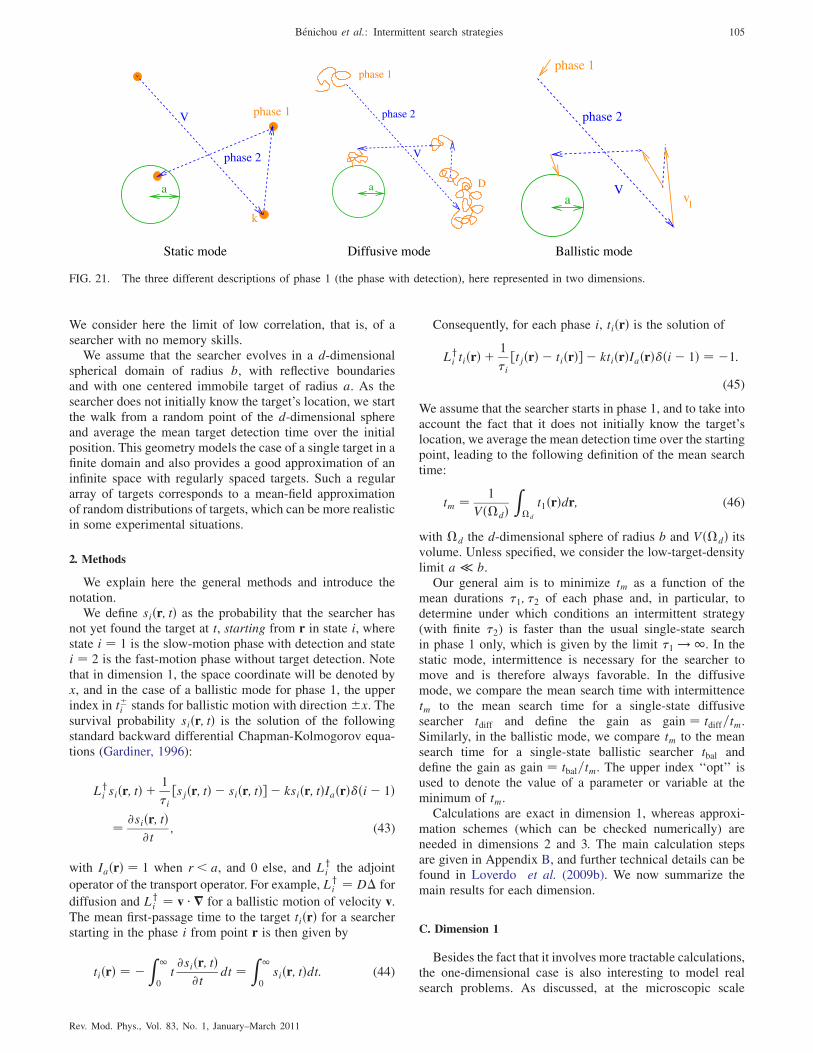
We consider here the limit of low correlation, that is, of asearcher with no memory skills.

We assume that the searcher evolves in a d-dimensionalspherical domain of radius b, with reflective boundariesand with one centered immobile target of radius a. As thesearcher does not initially know the target’s location, we startthe walk from a random point of the d-dimensional sphereand average the mean target detection time over the initialposition. This geometry models the case of a single target in afinite domain and also provides a good approximation of aninfinite space with regularly spaced targets. Such a regulararray of targets corresponds to a mean-field approximationof random distributions of targets, which can be more realisticin some experimental situations.

2. Methods

We explain here the general methods and introduce thenotation.

We define siðr; tÞ as the probability that the searcher hasnot yet found the target at t, starting from r in state i, wherestate i ¼ 1 is the slow-motion phase with detection and statei ¼ 2 is the fast-motion phase without target detection. Notethat in dimension 1, the space coordinate will be denoted byx, and in the case of a ballistic mode for phase 1, the upperindex in t i stands for ballistic motion with direction x. Thesurvival probability siðr; tÞ is the solution of the followingstandard backward differential Chapman-Kolmogorov equa-tions (Gardiner, 1996):

Lyi siðr; tÞ þ

1

�i½sjðr; tÞ � siðr; tÞ� � ksiðr; tÞIaðrÞ�ði� 1Þ

¼ @siðr; tÞ@t

; (43)

with IaðrÞ ¼ 1 when r < a, and 0 else, and Lyi the adjoint

operator of the transport operator. For example, Lyi ¼ D� for

diffusion and Lyi ¼ v � r for a ballistic motion of velocity v.

The mean first-passage time to the target tiðrÞ for a searcherstarting in the phase i from point r is then given by

tiðrÞ ¼ �Z 1

0t@siðr; tÞ

@tdt ¼

Z 1

0siðr; tÞdt: (44)

Consequently, for each phase i, tiðrÞ is the solution of

Lyi tiðrÞ þ

1

�i½tjðrÞ � tiðrÞ� � ktiðrÞIaðrÞ�ði� 1Þ ¼ �1:

(45)

We assume that the searcher starts in phase 1, and to take intoaccount the fact that it does not initially know the target’slocation, we average the mean detection time over the startingpoint, leading to the following definition of the mean searchtime:

tm ¼ 1

Vð�dÞZ�d

t1ðrÞdr; (46)

with �d the d-dimensional sphere of radius b and Vð�dÞ itsvolume. Unless specified, we consider the low-target-densitylimit a � b.

Our general aim is to minimize tm as a function of themean durations �1; �2 of each phase and, in particular, todetermine under which conditions an intermittent strategy(with finite �2) is faster than the usual single-state searchin phase 1 only, which is given by the limit �1 ! 1. In thestatic mode, intermittence is necessary for the searcher tomove and is therefore always favorable. In the diffusivemode, we compare the mean search time with intermittencetm to the mean search time for a single-state diffusivesearcher tdiff and define the gain as gain ¼ tdiff=tm.Similarly, in the ballistic mode, we compare tm to the meansearch time for a single-state ballistic searcher tbal anddefine the gain as gain ¼ tbal=tm. The upper index ‘‘opt’’ isused to denote the value of a parameter or variable at theminimum of tm.

Calculations are exact in dimension 1, whereas approxi-mation schemes (which can be checked numerically) areneeded in dimensions 2 and 3. The main calculation stepsare given in Appendix B, and further technical details can befound in Loverdo et al. (2009b). We now summarize themain results for each dimension.

C. Dimension 1

Besides the fact that it involves more tractable calculations,the one-dimensional case is also interesting to model realsearch problems. As discussed, at the microscopic scale

phase 2

V

a

phase 1

k

phase 2

V

phase 1

Da

phase 1

V

phase 2

a vl

Static mode Diffusive mode Ballistic mode

FIG. 21. The three different descriptions of phase 1 (the phase with detection), here represented in two dimensions.



tubular structures of cells such as axons or dendrites inneurons can be considered as one dimensional (Alberts,2002). The active transport of reactive particles, which alter-nate between diffusion phases and ballistic phases whenbound to molecular motors, can be schematically capturedby this generic model with diffusive mode (Loverdo et al.,2008). At the macroscopic scale, one could cite animals suchas ants (Dussutour et al., 2005), which tend to follow tracksor one-dimensional boundaries. More generally, borderlinesbetween different habitats, such as a shoreline, can be con-sidered as one dimensional.

It is shown in Appendix B that intermittent search strat-egies in dimension 1 share similar features for the static,diffusive, and ballistic detection modes. In particular, allmodes show regimes where intermittence is favorable andlead to a minimization of the search time. Strikingly, theoptimal duration of the nonreactive relocation phase 2 isquite independent of the modeling of the reactive phase:

�opt2 ¼ a

3V

ffiffiffiffiffiffiffiffiffib=a

pfor the static mode, for the ballistic mode

(in the regime vl < vcl ’ V

2

ffiffiffiffiffiffiffiffiffiffiffi3a=b

p), and for the diffusive

mode (in the regime b > DV and a � D

V

ffiffiffiffiffiffiffiffiffib=a

p). This shows

the robustness of the optimal value �opt2 .

D. Dimension 2

As discussed, the two-dimensional problem is particularlywell suited to model animal behaviors; it is also relevant tothe microscopic scale, since it mimics, for example, the caseof cellular traffic on membranes (Alberts, 2002). While indimension 1 the mean search time can be calculated analyti-cally, in dimension 2 (and later in dimension 3) approxima-tion schemes are necessary and can be checked by numericalsimulations.

Remarkably, for the three different modes of detection(static, diffusive, and ballistic), there is a regime whereintermittence minimizes the search time for one and the

same �opt2 , given by �

opt2 ¼ a

V

ffiffiffiffiffiffiffiffiffiffiffiffiffiffiffiffiffiffiffiffiffiffiffiffiffiffiffiffiffiffilnðb=aÞ � 1=2

p. As in dimen-

sion 1, this indicates that optimal intermittent strategiesare robust and widely independent of the details of thedescription of the detection mechanism.

E. Dimension 3

The three-dimensional case is also relevant to biology. Atthe microscopic scale, it corresponds, for example, to intra-cellular traffic in the bulk cytoplasm of cells, or at largerscales to animals living in dimension 3, such as plankton(Bartumeus et al., 2003) or Caenorhabditis elegans in itsnatural habitat (soil) (Kiontke and Sudhaus, 2005). As wasthe case in dimension 2, different assumptions have to bemade to obtain analytical expressions of the search time. Suchassumptions can be checked by numerical simulations usingthe same algorithms as in dimension 2.

For the three possible modelings of the detection mode(static, diffusive, and ballistic) in dimension 3, thereis a regime where the optimal strategy is intermittent.Remarkably, and as was the case in dimensions 1 and 2, theoptimal time to spend in the fast nonreactive phase 2 isindependent of the modeling of the detection mode and

reads �opt2 ’ 1:1 a

V . Additionally, while the mean first-passage

time to the target scales as b3, the optimal values of the

durations of the two phases do not depend on the target

density a=b.

F. Discussion and conclusion

To summarize, the methods of calculation developed

in this section and in Appendix B allow one to show that

the mean search time of intermittent random walks can be

minimized under broad conditions. Table I summarizes the

main results of this minimization. This study shows that the

optimal durations of the two phases and the gain of inter-

mittent search (as compared to a single-state search) do

depend on the target density in dimension 1. In particular,

the gain can be very high at low target concentration.

Interestingly, this dependence is smaller in dimension 2 and

vanishes in dimension 3. The fact that intermittent search

is more advantageous in low dimensions (1 and 2) can be

understood as follows. At large scale, the intermittent

searcher effectively performs a random walk, and therefore

scans a space of dimension 2. In an environment of dimen-

sion 1 (and marginally of dimension 2), the searcher therefore

oversamples the space, and it is favorable to perform large

jumps to go to previously unexplored areas. In contrast, in

dimension 3, the random walk is transient, and the searcher

on average always scans previously unexplored areas, which

makes large jumps less beneficial.Additionally, these results show that, for various modeling

choices of the slow reactive phase, there is one and the

same optimal duration of the fast nonreactive phase, which

depends only on the space dimension. This further supports

the robustness of optimal intermittent search strategies.

Such robustness and efficiency could explain why intermit-

tent trajectories are observed so often, as well as in various

forms.

V. EXTENSIONS AND PERSPECTIVES

Far from closing the problem, the generic model presented

in Sec. IV opens interesting perspectives. In this section, we

highlight a few promising directions: (i) The influence of the

targets’ distribution; and (ii) the effect of taking into account

a more involved searcher, enjoying now some orientational

and temporal memory. Indeed, in the generic model of

Sec. IV, the searcher has minimal memory skills. On the

one hand, the phase duration distribution is exponential,

which means that there is no temporal memory: The effect

of other duration distributions is studied in Sec. V.C. On the

other hand, the direction of each new ballistic blind phase is

taken at random, independently of the previous phases, mean-

ing that there is no orientational memory: We study the effect

of correlations in Sec. V.B. (iii) The effects of moving targets,

which can be more realistic at both the microscopic and

macroscopic scales. Next, we review in Sec. V.E similar

models of intermittent search, which have been proposed

recently in other contexts, and finally discuss how further

models could also be applied to design efficient searches

instead of interpreting biological systems (see Sec. V.F).



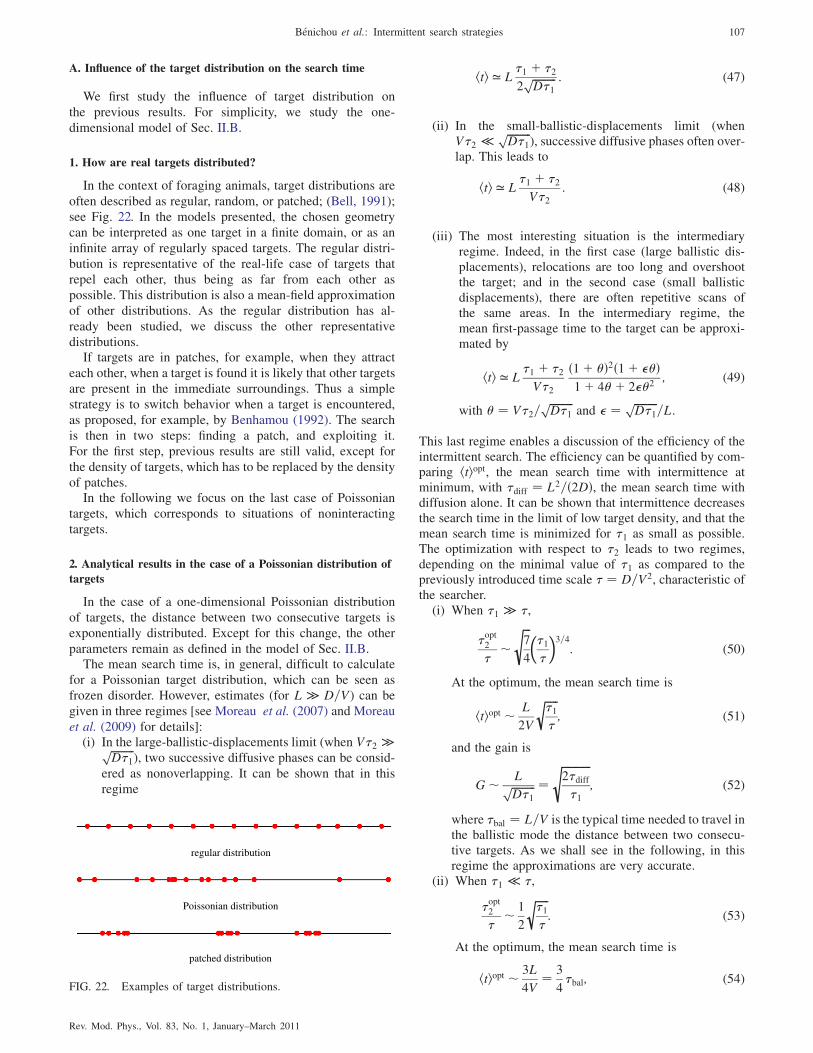
A. Influence of the target distribution on the search time

We first study the influence of target distribution on

the previous results. For simplicity, we study the one-

dimensional model of Sec. II.B.

1. How are real targets distributed?

In the context of foraging animals, target distributions are

often described as regular, random, or patched; (Bell, 1991);

see Fig. 22. In the models presented, the chosen geometry

can be interpreted as one target in a finite domain, or as an

infinite array of regularly spaced targets. The regular distri-

bution is representative of the real-life case of targets that

repel each other, thus being as far from each other as

possible. This distribution is also a mean-field approximation

of other distributions. As the regular distribution has al-

ready been studied, we discuss the other representative

distributions.If targets are in patches, for example, when they attract

each other, when a target is found it is likely that other targets

are present in the immediate surroundings. Thus a simple

strategy is to switch behavior when a target is encountered,

as proposed, for example, by Benhamou (1992). The search

is then in two steps: finding a patch, and exploiting it.

For the first step, previous results are still valid, except for

the density of targets, which has to be replaced by the density

of patches.In the following we focus on the last case of Poissonian

targets, which corresponds to situations of noninteracting

targets.

2. Analytical results in the case of a Poissonian distribution of

targets

In the case of a one-dimensional Poissonian distribution

of targets, the distance between two consecutive targets is

exponentially distributed. Except for this change, the other

parameters remain as defined in the model of Sec. II.B.The mean search time is, in general, difficult to calculate

for a Poissonian target distribution, which can be seen as

frozen disorder. However, estimates (for L � D=V) can be

given in three regimes [see Moreau et al. (2007) and Moreau

et al. (2009) for details]:(i) In the large-ballistic-displacements limit (when V�2 �ffiffiffiffiffiffiffiffiffi

D�1p

), two successive diffusive phases can be consid-

ered as nonoverlapping. It can be shown that in this

regime

hti ’ L�1 þ �22


p : (47)

(ii) In the small-ballistic-displacements limit (whenV�2 �


p), successive diffusive phases often over-

lap. This leads to

hti ’ L�1 þ �2V�2

: (48)

(iii) The most interesting situation is the intermediaryregime. Indeed, in the first case (large ballistic dis-placements), relocations are too long and overshootthe target; and in the second case (small ballisticdisplacements), there are often repetitive scans ofthe same areas. In the intermediary regime, themean first-passage time to the target can be approxi-mated by

hti ’ L�1 þ �2V�2

ð1þ �Þ2ð1þ ��Þ1þ 4�þ 2��2

; (49)

with � ¼ V�2=ffiffiffiffiffiffiffiffiffiD�1

pand � ¼ ffiffiffiffiffiffiffiffiffi

D�1p

=L.

This last regime enables a discussion of the efficiency of theintermittent search. The efficiency can be quantified by com-paring htiopt, the mean search time with intermittence atminimum, with �diff ¼ L2=ð2DÞ, the mean search time withdiffusion alone. It can be shown that intermittence decreasesthe search time in the limit of low target density, and that themean search time is minimized for �1 as small as possible.The optimization with respect to �2 leads to two regimes,depending on the minimal value of �1 as compared to thepreviously introduced time scale � ¼ D=V2, characteristic ofthe searcher.

(i) When �1 � �,

�opt2

��

ffiffiffi7

4

s ��1�

�3=4

: (50)

At the optimum, the mean search time is

htiopt � L

2V

ffiffiffiffiffi�1�

r; (51)

and the gain is

G� LffiffiffiffiffiffiffiffiffiD�1

p ¼ffiffiffiffiffiffiffiffiffiffiffi2�diff�1

s; (52)

where �bal ¼ L=V is the typical time needed to travel inthe ballistic mode the distance between two consecu-tive targets. As we shall see in the following, in thisregime the approximations are very accurate.

(ii) When �1 � �,

�opt2

�� 1

2

ffiffiffiffiffi�1�

r: (53)

At the optimum, the mean search time is

htiopt � 3L

4V¼ 3

4�bal; (54)

regular distribution

Poissonian distribution

patched distribution

FIG. 22. Examples of target distributions.



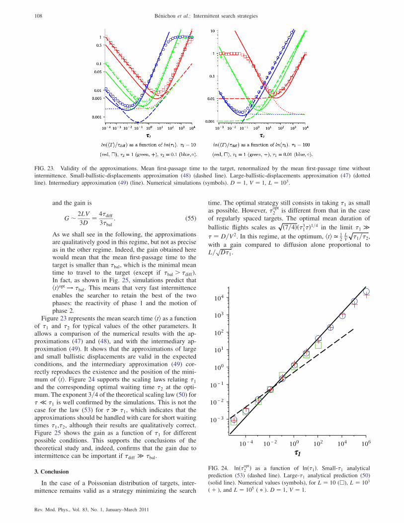
and the gain is

G� 2LV

3D¼ 4�diff

3�bal: (55)

As we shall see in the following, the approximationsare qualitatively good in this regime, but not as preciseas in the other regime. Indeed, the gain obtained herewould mean that the mean first-passage time to thetarget is smaller than �bal, which is the minimal meantime to travel to the target (except if �bal > �diff).In fact, as shown in Fig. 25, simulations predict thathtiopt ! �bal. This means that very fast intermittenceenables the searcher to retain the best of the twophases: the reactivity of phase 1 and the motion ofphase 2.

Figure 23 represents the mean search time hti as a functionof �1 and �2 for typical values of the other parameters. Itallows a comparison of the numerical results with the ap-proximations (47) and (48), and with the intermediary ap-proximation (49). It shows that the approximations of largeand small ballistic displacements are valid in the expectedconditions, and the intermediary approximation (49) cor-rectly reproduces the existence and the position of the mini-mum of hti. Figure 24 supports the scaling laws relating �1and the corresponding optimal waiting time �2 at the opti-mum. The exponent 3=4 of the theoretical scaling law (50) for� � �1 is well confirmed by the simulations. This is not thecase for the law (53) for � � �1, which indicates that theapproximations should be handled with care for short waitingtimes �1,�2, although their results are qualitatively correct.Figure 25 shows the gain as a function of �1 for differentpossible conditions. This supports the conclusions of thetheoretical study and, indeed, confirms that the gain due tointermittence can be important if �diff � �bal.

3. Conclusion

In the case of a Poissonian distribution of targets, inter-mittence remains valid as a strategy minimizing the search

time. The optimal strategy still consists in taking �1 as smallas possible. However, �

opt2 is different from that in the case

of regularly spaced targets. The optimal mean duration of

ballistic flights scales asffiffiffiffiffiffiffiffiffiffiffið7=4Þp ð�31�Þ1=4 in the limit �1 �

� ¼ D=V2. In this regime, at the optimum, hti ’ 12

LV

ffiffiffiffiffiffiffiffiffiffiffiffi�1=�2

p,

with a gain compared to diffusion alone proportional toL=


p.

FIG. 23. Validity of the approximations. Mean first-passage time to the target, renormalized by the mean first-passage time without

intermittence. Small-ballistic-displacements approximation (48) (dashed line). Large-ballistic-displacements approximation (47) (dotted

line). Intermediary approximation (49) (line). Numerical simulations (symbols). D ¼ 1, V ¼ 1, L ¼ 103.

FIG. 24. lnð�opt2 Þ as a function of lnð�1Þ. Small-�1 analytical

prediction (53) (dashed line). Large-�1 analytical prediction (50)

(solid line). Numerical values (symbols), for L ¼ 10 (h), L ¼ 103

(þ ), and L ¼ 105 ( � ). D ¼ 1, V ¼ 1.



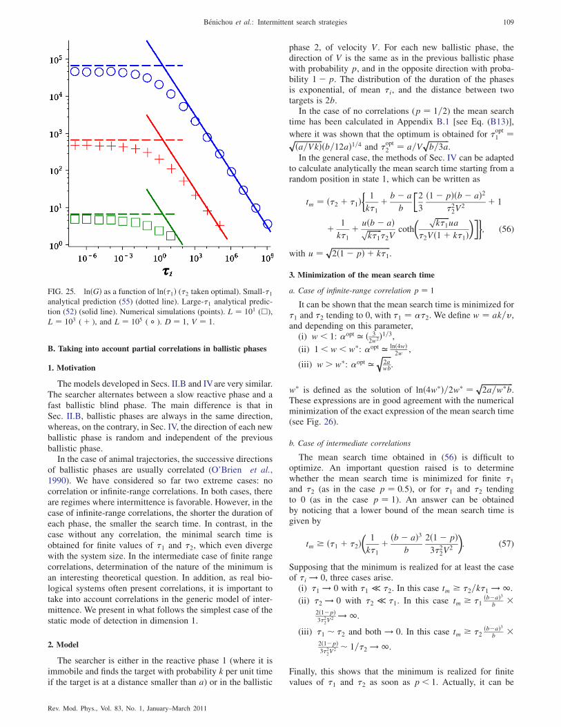
B. Taking into account partial correlations in ballistic phases

1. Motivation

The models developed in Secs. II.B and IVare very similar.

The searcher alternates between a slow reactive phase and a

fast ballistic blind phase. The main difference is that in

Sec. II.B, ballistic phases are always in the same direction,

whereas, on the contrary, in Sec. IV, the direction of each new

ballistic phase is random and independent of the previous

ballistic phase.In the case of animal trajectories, the successive directions

of ballistic phases are usually correlated (O’Brien et al.,

1990). We have considered so far two extreme cases: no

correlation or infinite-range correlations. In both cases, there

are regimes where intermittence is favorable. However, in the

case of infinite-range correlations, the shorter the duration of

each phase, the smaller the search time. In contrast, in the

case without any correlation, the minimal search time is

obtained for finite values of �1 and �2, which even diverge

with the system size. In the intermediate case of finite range

correlations, determination of the nature of the minimum is

an interesting theoretical question. In addition, as real bio-

logical systems often present correlations, it is important to

take into account correlations in the generic model of inter-

mittence. We present in what follows the simplest case of the

static mode of detection in dimension 1.

2. Model

The searcher is either in the reactive phase 1 (where it is

immobile and finds the target with probability k per unit time

if the target is at a distance smaller than a) or in the ballistic

phase 2, of velocity V. For each new ballistic phase, thedirection of V is the same as in the previous ballistic phasewith probability p, and in the opposite direction with proba-bility 1� p. The distribution of the duration of the phasesis exponential, of mean �i, and the distance between twotargets is 2b.

In the case of no correlations (p ¼ 1=2) the mean searchtime has been calculated in Appendix B.1 [see Eq. (B13)],

where it was shown that the optimum is obtained for �opt1 ¼ffiffiffiffiffiffiffiffiffiffiffiffiffiffiffiða=VkÞp ðb=12aÞ1=4 and �

opt2 ¼ a=V

ffiffiffiffiffiffiffiffiffiffiffib=3a

p.

In the general case, the methods of Sec. IV can be adaptedto calculate analytically the mean search time starting from arandom position in state 1, which can be written as

tm ¼ ð�2 þ �1Þ�1

k�1þ b� a

b

�2

3

ð1� pÞðb� aÞ2�22V

2þ 1

þ 1

k�1þ uðb� aÞffiffiffiffiffiffiffiffi

k�1p

�2Vcoth

� ffiffiffiffiffiffiffiffik�1

pua

�2Vð1þ k�1Þ��

; (56)

with u ¼ ffiffiffiffiffiffiffiffiffiffiffiffiffiffiffiffiffiffiffiffiffiffiffiffiffiffiffiffiffiffiffiffi2ð1� pÞ þ k�1

p.

3. Minimization of the mean search time

a. Case of infinite-range correlation p ¼ 1

It can be shown that the mean search time is minimized for�1 and �2 tending to 0, with �1 ¼ ��2. We define w ¼ ak=v,and depending on this parameter,

(i) w< 1: �opt ’ ð 32w2Þ1=3,

(ii) 1<w<w�: �opt ’ lnð4wÞ2w ,

(iii) w> w�: �opt ’ffiffiffiffiffi2awb

q.

w� is defined as the solution of lnð4w�Þ=2w� ¼ ffiffiffiffiffiffiffiffiffiffiffiffiffiffiffiffiffi2a=w�b

p.

These expressions are in good agreement with the numericalminimization of the exact expression of the mean search time(see Fig. 26).

b. Case of intermediate correlations

The mean search time obtained in (56) is difficult tooptimize. An important question raised is to determinewhether the mean search time is minimized for finite �1and �2 (as in the case p ¼ 0:5), or for �1 and �2 tendingto 0 (as in the case p ¼ 1). An answer can be obtainedby noticing that a lower bound of the mean search time isgiven by

tm � ð�1 þ �2Þ�1

k�1þ ðb� aÞ3

b

2ð1� pÞ3�22V

2

�: (57)

Supposing that the minimum is realized for at least the caseof �i ! 0, three cases arise.

(i) �1 ! 0 with �1 � �2. In this case tm � �2=k�1 ! 1.

(ii) �2 ! 0 with �2 � �1. In this case tm � �1ðb�aÞ3

b 2ð1�pÞ3�2

2V2 ! 1.

(iii) �1 � �2 and both ! 0. In this case tm � �2ðb�aÞ3

b 2ð1�pÞ3�2

2V2 � 1=�2 ! 1.

Finally, this shows that the minimum is realized for finitevalues of �1 and �2 as soon as p < 1. Actually, it can be

FIG. 25. lnðGÞ as a function of lnð�1Þ (�2 taken optimal). Small-�1analytical prediction (55) (dotted line). Large-�1 analytical predic-

tion (52) (solid line). Numerical simulations (points). L ¼ 101 (h),

L ¼ 103 (þ ), and L ¼ 105 ( � ). D ¼ 1, V ¼ 1.



shown that, except for p close to 1, the minimum of thesearch time is obtained for

�opt1 ¼

ffiffiffiffiffiffia

Vk

r �b

a

ð1� pÞ6

�1=4

(58)

and

�opt2 ¼ a

V

ffiffiffiffiffiffiffiffiffiffiffiffiffiffiffiffiffiffiffiffiffiffiffib

a

2ð1� pÞ3

s: (59)

Interestingly, note that the relation �opt2 ¼ 2kð�opt1 Þ2 obtained

initially in the case of the absence of correlations (see Table I)still holds in this case.

These expressions are in agreement with the numericalminimization of the exact expression of the mean search time(see Fig. 27), except when 1� p is very small.

4. Conclusion

In the simple case of the static mode in one dimension,the influence of correlations on the mean search time and itsminimization can be studied. An exact expression for themean search time shows that it is minimized for finite valuesof �1 and �2 as soon as p < 1. When 1� p � a=b, theoptimal durations �

opt1 and �

opt2 can be explicitly given, and

they are in continuity with the case without correlation,p ¼ 0:5.

C. Other distributions of phase durations

The model presented in Sec. IV is minimal in the sense thatthe searcher has no memory. As seen in the previous section,one possibility is to add orientational memory. Another pos-sibility is to add temporal memory. In the generic model, wehave considered a ‘‘Markovian’’ searcher, in the sense thatthe rate of switching from one phase to the other is constant.It leads to an exponential distribution of the durations ofthe phases. In the following, we study the influence of thedistribution of the duration of the phases [see also Chechkinet al. (2009), Meerschaert et al. (2009), and Tejedor andMetzler (2009) for other types of correlation]. A first possi-bility is to study the effect of distributions that are peakedaround the mean duration, or even deterministic (Benichouet al., 2007). A second possibility is to study the case ofLevy-distributed blind phases as in Lomholt et al. (2008).

1. Deterministic durations of the phases

In the generic model described, we considered exponentialdurations of phases, which correspond to searchers with notemporal memory. In the opposite case, a searcher with full

FIG. 26. Minimization of the mean search time for the static

mode with infinite correlation (p ¼ 1). �opt as a function of w.Theoretical expression for small w (dots), for intermediate w (solid

line), and for large w (dashed lines). Optimization of the exact

expression (with �2 ! 0 and �1 ¼ ��2) (symbols). b ¼ 100 (h),

b ¼ 103 (þ ), b ¼ 104 (�), and b ¼ 105 ( ? ). a ¼ 1, V ¼ 1.

FIG. 27. �opt as a function of 2ð1� pÞ. Theoretical value of �opt1 (58) (dashed line) and theoretical value of �opt2 (59) (solid lines), compared

to the numerical minimization of the full exact mean search time, leading to �opt1 (filled symbols) and �opt2 (empty symbols). a ¼ 0:01, b ¼ 1

(4); a ¼ 0:01, b ¼ 100 (h); a ¼ 1, b ¼ 100 (�); a ¼ 1, b ¼ 104 (w); a ¼ 100, b ¼ 104 (5); a ¼ 100, b ¼ 106 (e). k ¼ 1, V ¼ 1.



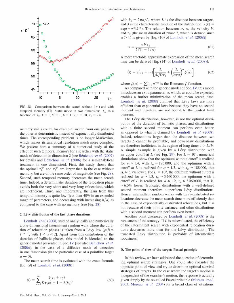
memory skills could, for example, switch from one phase tothe other at deterministic instead of exponentially distributedtimes. The corresponding problem is no longer Markovian,which makes its analytical resolution much more complex.We present here a summary of a numerical study of theeffect of such temporal memory for a searcher with the staticmode of detection in dimension 2 [see Benichou et al. (2007)for details and Benichou et al. (2006) for a semianalyticaltreatment in one dimension]. First, this study shows thatthe optimal �

opt1 and �

opt2 are larger than in the case without

memory, but are of the same order of magnitude (see Fig. 28).Second, such temporal memory decreases the mean searchtime. Indeed, a deterministic duration of the relocation phaseavoids both the very short and very long relocations, whichare inefficient. Third, and importantly, the gain from thistemporal memory is quite low (less than 40% in an extendedrange of parameters, and decreasing with increasing b=a) ascompared to the case with no memory (see Fig. 28).

2. Levy distribution of the fast phase durations

Lomholt et al. (2008) studied analytically and numericallya one-dimensional intermittent random walk where the dura-tion of relocation phases is taken from a Levy law [pðlÞ /l��1, with 1<�< 2]. Apart from this distribution of theduration of ballistic phases, this model is identical to thegeneric model presented in Sec. IV [see also Benichou et al.(2006)], in the case of a diffusive mode of detectionin one dimension (in the particular case of a pointlike targeta ! 0).

The mean search time is evaluated with the exact formula[Eq. (9) of Lomholt et al. (2008)]

hti ¼ X1n¼1

2ð�1 þ �2ÞD�1k

2n þ 1� �ðknÞ

; (60)

with kn ¼ 2�n=L, where L is the distance between targets,and � is the characteristic function of the distribution: �ðkÞ ¼expð��jkj�Þ. The relation between , �, the velocity V,and �2 (the mean duration of phase 2, which is defined since� > 1) is given by [Eq. (10) of Lomholt et al. (2008)]

¼ �V�22�ð1� 1=�Þ : (61)

A more tractable approximate expression of the mean searchtime can be derived [Eq. (14) of Lomholt et al. (2008)]:

hti ¼ 2ð�1 þ �2Þ�

L

4ffiffiffiffiffiffiffiffiffiD�1

p þ�

L

2�

��ð�Þ

�; (62)

where �ð�Þ ¼ P1n¼1 n

�� is the Riemann � function.

As compared with the generic model of Sec. IV, this modelintroduces an extra parameter �, which, as could be expected,enables a further minimization of the mean search time.Lomholt et al. (2008) claimed that Levy laws are moreefficient than exponential laws because they have no secondmoment and therefore are not bound to the central limittheorem.

The Levy distribution, however, is not the optimal distri-bution of the duration of ballistic phases, and distributionswith a finite second moment can perform even better,as opposed to what is claimed by Lomholt et al. (2008).Indeed, relocations larger than the distance between twotargets L cannot be profitable, and power-law distributionsare therefore inefficient in the regime of long times t > L=V.A simple example is given by a Levy distribution withan upper cutoff at L (see Fig. 29). For L ¼ 104, numericalsimulations show that the optimum without cutoff is realizedfor � ’ 1:4, with tm ’ 195 000, and the optimum with acutoff at L is realized for � ’ 1:3, with tm ’ 188 000, thatis, ’ 3:7% lower. For L ¼ 105, the optimum without cutoff isrealized for � ’ 1:3, tm ’ 3 260 000; the optimum with acutoff of L is realized for � ’ 1:2, tm ’ 3 060 000, that is,’ 6:5% lower. Truncated distributions with a well-definedsecond moment therefore outperform Levy distributions.Hence, intermittent random walks with Levy-distributed re-locations decrease the mean search time more efficiently thanin the case of exponentially distributed relocations, but it isnot because of their infinite variance, and other distributionswith a second moment can perform even better.

Another point discussed by Lomholt et al. (2008) is therobustness of the strategy: If L is misevaluated, the efficiencyof the intermittent search with exponential relocation dura-tions decreases more than for the Levy distribution. Thetruncated Levy distribution is probably of intermediaterobustness.

D. The point of view of the target: Pascal principle

In this review, we have addressed the question of determin-ing optimal search strategies. One could also consider theopposite point of view and try to determine optimal survivalstrategies of targets. In the case where the target’s motion isindependent of the searcher’s motion, the response is actuallygiven simply by the so-called Pascal principle (Moreau et al.,2003; Moreau et al., 2004) for a broad class of situations.

FIG. 28. Comparison between the search without ( � ) and with

temporal memory (h). Static mode in two dimensions. tm as a

function of �2. k ¼ 1, V ¼ 1, b ¼ 113, a ¼ 10, �1 ¼ 2:6.



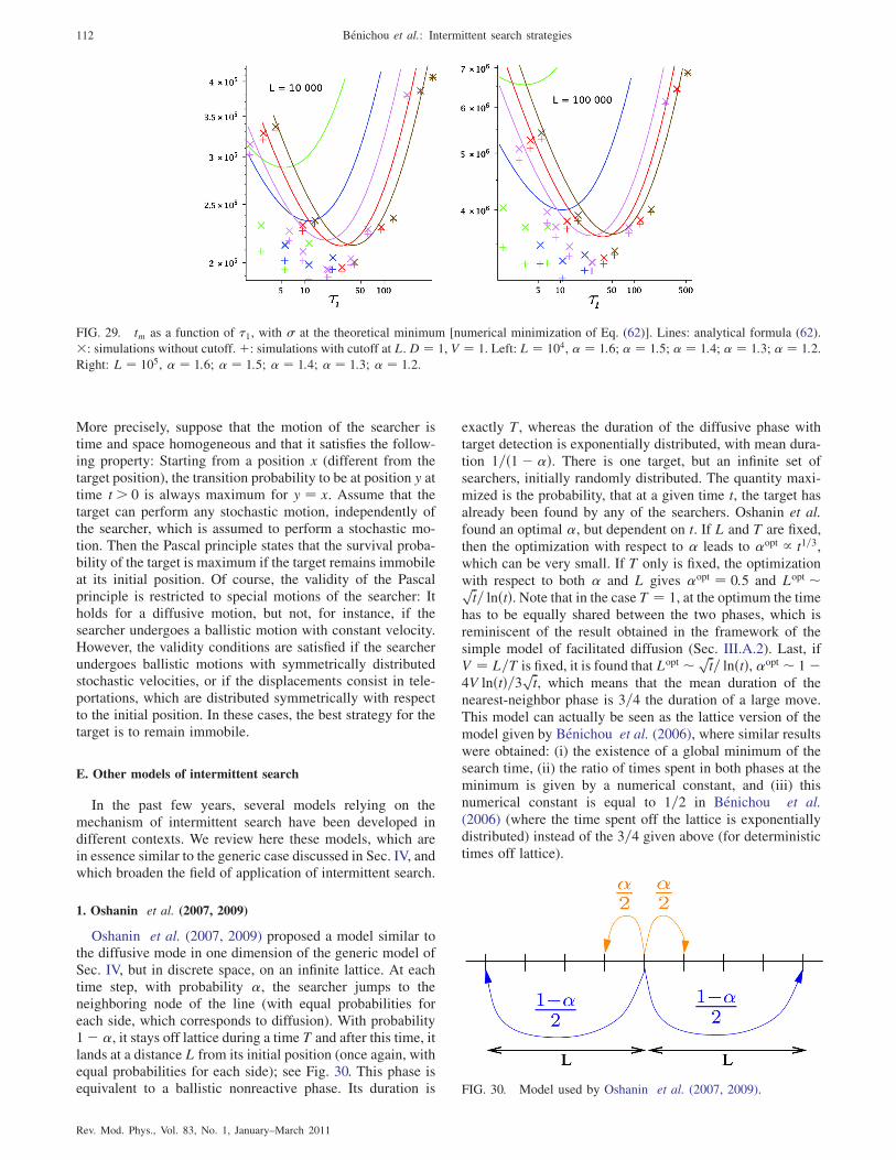
More precisely, suppose that the motion of the searcher istime and space homogeneous and that it satisfies the follow-ing property: Starting from a position x (different from thetarget position), the transition probability to be at position y attime t > 0 is always maximum for y ¼ x. Assume that thetarget can perform any stochastic motion, independently ofthe searcher, which is assumed to perform a stochastic mo-tion. Then the Pascal principle states that the survival proba-bility of the target is maximum if the target remains immobileat its initial position. Of course, the validity of the Pascalprinciple is restricted to special motions of the searcher: Itholds for a diffusive motion, but not, for instance, if thesearcher undergoes a ballistic motion with constant velocity.However, the validity conditions are satisfied if the searcherundergoes ballistic motions with symmetrically distributedstochastic velocities, or if the displacements consist in tele-portations, which are distributed symmetrically with respectto the initial position. In these cases, the best strategy for thetarget is to remain immobile.

E. Other models of intermittent search

In the past few years, several models relying on themechanism of intermittent search have been developed indifferent contexts. We review here these models, which arein essence similar to the generic case discussed in Sec. IV, andwhich broaden the field of application of intermittent search.

1. Oshanin et al. (2007, 2009)

Oshanin et al. (2007, 2009) proposed a model similar tothe diffusive mode in one dimension of the generic model ofSec. IV, but in discrete space, on an infinite lattice. At eachtime step, with probability �, the searcher jumps to theneighboring node of the line (with equal probabilities foreach side, which corresponds to diffusion). With probability1� �, it stays off lattice during a time T and after this time, itlands at a distance L from its initial position (once again, withequal probabilities for each side); see Fig. 30. This phase isequivalent to a ballistic nonreactive phase. Its duration is

exactly T, whereas the duration of the diffusive phase withtarget detection is exponentially distributed, with mean dura-tion 1=ð1� �Þ. There is one target, but an infinite set of

searchers, initially randomly distributed. The quantity maxi-mized is the probability, that at a given time t, the target hasalready been found by any of the searchers. Oshanin et al.

found an optimal �, but dependent on t. If L and T are fixed,then the optimization with respect to � leads to �opt / t1=3,which can be very small. If T only is fixed, the optimization

with respect to both � and L gives �opt ¼ 0:5 and Lopt �ffiffit

p= lnðtÞ. Note that in the case T ¼ 1, at the optimum the time

has to be equally shared between the two phases, which is

reminiscent of the result obtained in the framework of thesimple model of facilitated diffusion (Sec. III.A.2). Last, ifV ¼ L=T is fixed, it is found that Lopt � ffiffi

tp

= lnðtÞ,�opt � 1�4V lnðtÞ=3 ffiffi

tp

, which means that the mean duration of thenearest-neighbor phase is 3=4 the duration of a large move.This model can actually be seen as the lattice version of the

model given by Benichou et al. (2006), where similar resultswere obtained: (i) the existence of a global minimum of the

search time, (ii) the ratio of times spent in both phases at theminimum is given by a numerical constant, and (iii) thisnumerical constant is equal to 1=2 in Benichou et al.

(2006) (where the time spent off the lattice is exponentiallydistributed) instead of the 3=4 given above (for deterministictimes off lattice).

FIG. 29. tm as a function of �1, with at the theoretical minimum [numerical minimization of Eq. (62)]. Lines: analytical formula (62).

: simulations without cutoff.þ: simulations with cutoff at L. D ¼ 1, V ¼ 1. Left: L ¼ 104, � ¼ 1:6; � ¼ 1:5; � ¼ 1:4; � ¼ 1:3; � ¼ 1:2.Right: L ¼ 105, � ¼ 1:6; � ¼ 1:5; � ¼ 1:4; � ¼ 1:3; � ¼ 1:2.

FIG. 30. Model used by Oshanin et al. (2007, 2009).



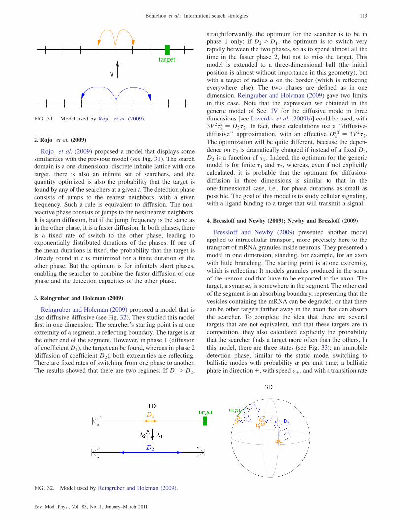
2. Rojo et al. (2009)

Rojo et al. (2009) proposed a model that displays somesimilarities with the previous model (see Fig. 31). The searchdomain is a one-dimensional discrete infinite lattice with onetarget, there is also an infinite set of searchers, and thequantity optimized is also the probability that the target isfound by any of the searchers at a given t. The detection phaseconsists of jumps to the nearest neighbors, with a givenfrequency. Such a rule is equivalent to diffusion. The non-reactive phase consists of jumps to the next nearest neighbors.It is again diffusion, but if the jump frequency is the same asin the other phase, it is a faster diffusion. In both phases, thereis a fixed rate of switch to the other phase, leading toexponentially distributed durations of the phases. If one ofthe mean durations is fixed, the probability that the target is

already found at t is minimized for a finite duration of theother phase. But the optimum is for infinitely short phases,enabling the searcher to combine the faster diffusion of onephase and the detection capacities of the other phase.

3. Reingruber and Holcman (2009)

Reingruber and Holcman (2009) proposed a model that isalso diffusive-diffusive (see Fig. 32). They studied this modelfirst in one dimension: The searcher’s starting point is at oneextremity of a segment, a reflecting boundary. The target is atthe other end of the segment. However, in phase 1 (diffusionof coefficientD1), the target can be found, whereas in phase 2(diffusion of coefficient D2), both extremities are reflecting.There are fixed rates of switching from one phase to another.The results showed that there are two regimes: If D1 >D2,

straightforwardly, the optimum for the searcher is to be in

phase 1 only; if D2 >D1, the optimum is to switch very

rapidly between the two phases, so as to spend almost all the

time in the faster phase 2, but not to miss the target. This

model is extended to a three-dimensional ball (the initial

position is almost without importance in this geometry), but

with a target of radius a on the border (which is reflecting

everywhere else). The two phases are defined as in one

dimension. Reingruber and Holcman (2009) gave two limits

in this case. Note that the expression we obtained in the

generic model of Sec. IV for the diffusive mode in three

dimensions [see Loverdo et al. (2009b)] could be used, with

3V2�22 ¼ D2�2. In fact, these calculations use a ‘‘diffusive-

diffusive’’ approximation, with an effective Deff2 ¼ 3V2�2.

The optimization will be quite different, because the depen-

dence on �2 is dramatically changed if instead of a fixed D2,

D2 is a function of �2. Indeed, the optimum for the generic

model is for finite �1 and �2, whereas, even if not explicitly

calculated, it is probable that the optimum for diffusion-

diffusion in three dimensions is similar to that in the

one-dimensional case, i.e., for phase durations as small as

possible. The goal of this model is to study cellular signaling,

with a ligand binding to a target that will transmit a signal.

4. Bressloff and Newby (2009); Newby and Bressloff (2009)

Bressloff and Newby (2009) presented another model

applied to intracellular transport, more precisely here to the

transport of mRNA granules inside neurons. They presented a

model in one dimension, standing, for example, for an axon

with little branching. The starting point is at one extremity,

which is reflecting: It models granules produced in the soma

of the neuron and that have to be exported to the axon. The

target, a synapse, is somewhere in the segment. The other end

of the segment is an absorbing boundary, representing that the

vesicles containing the mRNA can be degraded, or that there

can be other targets farther away in the axon that can absorb

the searcher. To complete the idea that there are several

targets that are not equivalent, and that these targets are in

competition, they also calculated explicitly the probability

that the searcher finds a target more often than the others. In

this model, there are three states (see Fig. 33): an immobile

detection phase, similar to the static mode, switching to

ballistic modes with probability � per unit time; a ballistic

phase in directionþ, with speed vþ, and with a transition rate

target

FIG. 31. Model used by Rojo et al. (2009).

FIG. 32. Model used by Reingruber and Holcman (2009).



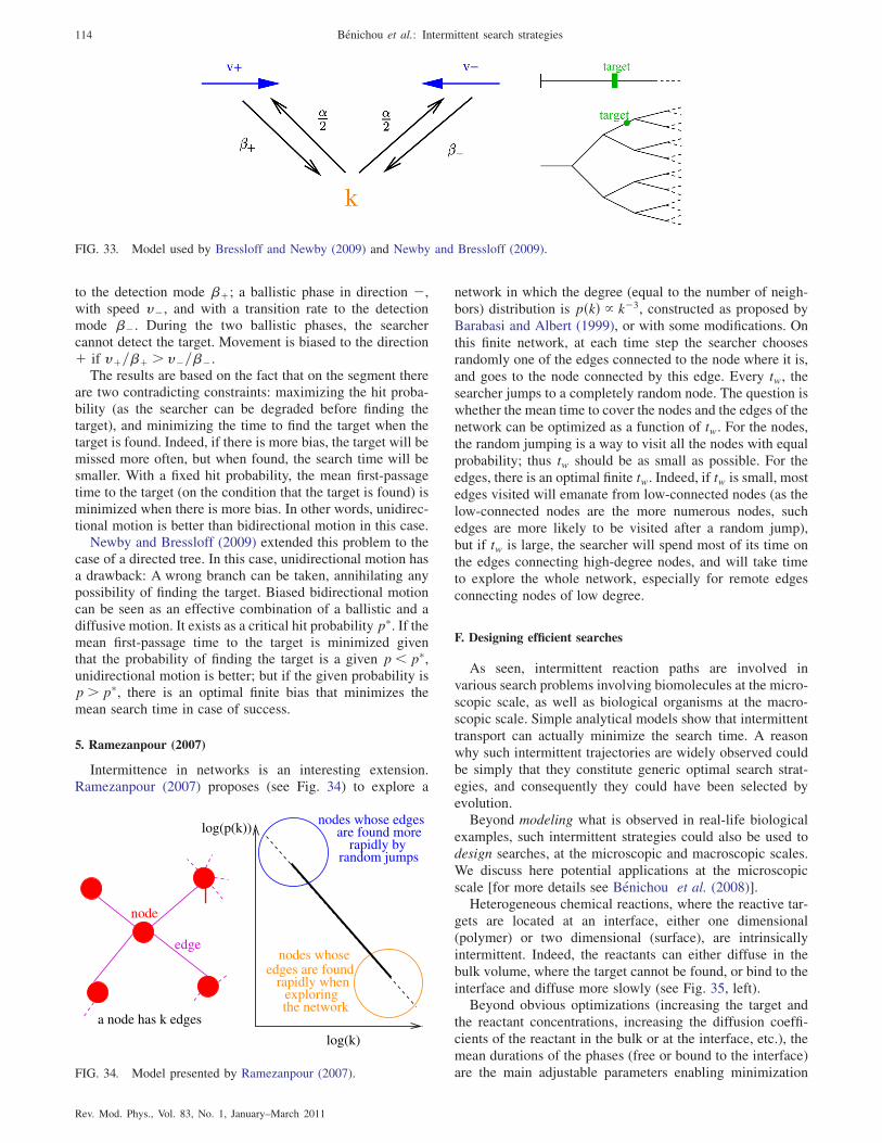
to the detection mode �þ; a ballistic phase in direction �,with speed v�, and with a transition rate to the detectionmode ��. During the two ballistic phases, the searchercannot detect the target. Movement is biased to the directionþ if vþ=�þ > v�=��.

The results are based on the fact that on the segment thereare two contradicting constraints: maximizing the hit proba-bility (as the searcher can be degraded before finding thetarget), and minimizing the time to find the target when thetarget is found. Indeed, if there is more bias, the target will bemissed more often, but when found, the search time will besmaller. With a fixed hit probability, the mean first-passagetime to the target (on the condition that the target is found) isminimized when there is more bias. In other words, unidirec-tional motion is better than bidirectional motion in this case.

Newby and Bressloff (2009) extended this problem to thecase of a directed tree. In this case, unidirectional motion hasa drawback: A wrong branch can be taken, annihilating anypossibility of finding the target. Biased bidirectional motioncan be seen as an effective combination of a ballistic and adiffusive motion. It exists as a critical hit probability p�. If themean first-passage time to the target is minimized giventhat the probability of finding the target is a given p < p�,unidirectional motion is better; but if the given probability isp > p�, there is an optimal finite bias that minimizes themean search time in case of success.

5. Ramezanpour (2007)

Intermittence in networks is an interesting extension.Ramezanpour (2007) proposes (see Fig. 34) to explore a

network in which the degree (equal to the number of neigh-

bors) distribution is pðkÞ / k�3, constructed as proposed by

Barabasi and Albert (1999), or with some modifications. On

this finite network, at each time step the searcher chooses

randomly one of the edges connected to the node where it is,

and goes to the node connected by this edge. Every tw, thesearcher jumps to a completely random node. The question is

whether the mean time to cover the nodes and the edges of the

network can be optimized as a function of tw. For the nodes,the random jumping is a way to visit all the nodes with equal

probability; thus tw should be as small as possible. For the

edges, there is an optimal finite tw. Indeed, if tw is small, most

edges visited will emanate from low-connected nodes (as the

low-connected nodes are the more numerous nodes, such

edges are more likely to be visited after a random jump),

but if tw is large, the searcher will spend most of its time on

the edges connecting high-degree nodes, and will take time

to explore the whole network, especially for remote edges

connecting nodes of low degree.

F. Designing efficient searches

As seen, intermittent reaction paths are involved in

various search problems involving biomolecules at the micro-

scopic scale, as well as biological organisms at the macro-

scopic scale. Simple analytical models show that intermittent

transport can actually minimize the search time. A reason

why such intermittent trajectories are widely observed could

be simply that they constitute generic optimal search strat-

egies, and consequently they could have been selected by

evolution.Beyond modeling what is observed in real-life biological

examples, such intermittent strategies could also be used to

design searches, at the microscopic and macroscopic scales.

We discuss here potential applications at the microscopic

scale [for more details see Benichou et al. (2008)].Heterogeneous chemical reactions, where the reactive tar-

gets are located at an interface, either one dimensional

(polymer) or two dimensional (surface), are intrinsically

intermittent. Indeed, the reactants can either diffuse in the

bulk volume, where the target cannot be found, or bind to the

interface and diffuse more slowly (see Fig. 35, left).Beyond obvious optimizations (increasing the target and

the reactant concentrations, increasing the diffusion coeffi-

cients of the reactant in the bulk or at the interface, etc.), the

mean durations of the phases (free or bound to the interface)

are the main adjustable parameters enabling minimization

FIG. 33. Model used by Bressloff and Newby (2009) and Newby and Bressloff (2009).

edge

node

a node has k edges

log(p(k))

log(k)

nodes whoseedges are found

rapidly when exploringthe network

nodes whose edgesare found more

rapidly by random jumps

FIG. 34. Model presented by Ramezanpour (2007).



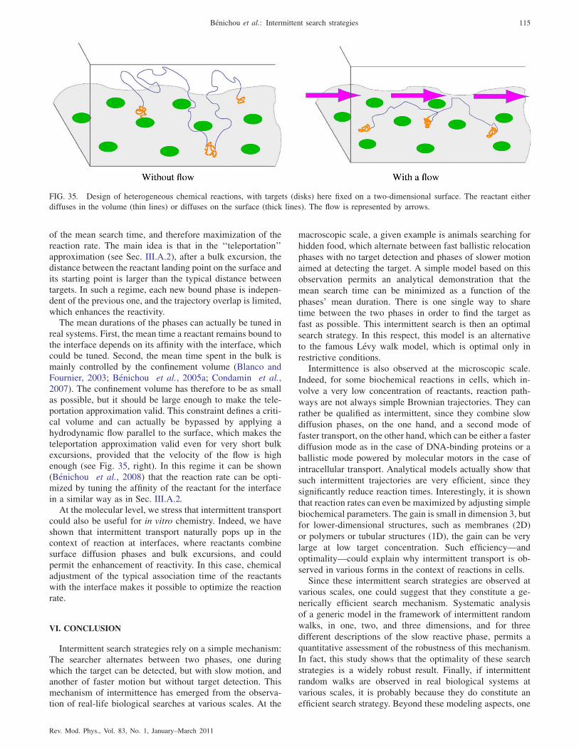
of the mean search time, and therefore maximization of thereaction rate. The main idea is that in the ‘‘teleportation’’approximation (see Sec. III.A.2), after a bulk excursion, thedistance between the reactant landing point on the surface andits starting point is larger than the typical distance betweentargets. In such a regime, each new bound phase is indepen-dent of the previous one, and the trajectory overlap is limited,

which enhances the reactivity.The mean durations of the phases can actually be tuned in

real systems. First, the mean time a reactant remains bound tothe interface depends on its affinity with the interface, whichcould be tuned. Second, the mean time spent in the bulk ismainly controlled by the confinement volume (Blanco andFournier, 2003; Benichou et al., 2005a; Condamin et al.,2007). The confinement volume has therefore to be as smallas possible, but it should be large enough to make the tele-portation approximation valid. This constraint defines a criti-cal volume and can actually be bypassed by applying ahydrodynamic flow parallel to the surface, which makes the

teleportation approximation valid even for very short bulkexcursions, provided that the velocity of the flow is highenough (see Fig. 35, right). In this regime it can be shown(Benichou et al., 2008) that the reaction rate can be opti-mized by tuning the affinity of the reactant for the interfacein a similar way as in Sec. III.A.2.

At the molecular level, we stress that intermittent transportcould also be useful for in vitro chemistry. Indeed, we haveshown that intermittent transport naturally pops up in thecontext of reaction at interfaces, where reactants combinesurface diffusion phases and bulk excursions, and couldpermit the enhancement of reactivity. In this case, chemicaladjustment of the typical association time of the reactants

with the interface makes it possible to optimize the reactionrate.

VI. CONCLUSION

Intermittent search strategies rely on a simple mechanism:The searcher alternates between two phases, one duringwhich the target can be detected, but with slow motion, andanother of faster motion but without target detection. Thismechanism of intermittence has emerged from the observa-tion of real-life biological searches at various scales. At the

macroscopic scale, a given example is animals searching for

hidden food, which alternate between fast ballistic relocation

phases with no target detection and phases of slower motion

aimed at detecting the target. A simple model based on this

observation permits an analytical demonstration that the

mean search time can be minimized as a function of the

phases’ mean duration. There is one single way to share

time between the two phases in order to find the target as

fast as possible. This intermittent search is then an optimal

search strategy. In this respect, this model is an alternative

to the famous Levy walk model, which is optimal only in

restrictive conditions.Intermittence is also observed at the microscopic scale.

Indeed, for some biochemical reactions in cells, which in-

volve a very low concentration of reactants, reaction path-

ways are not always simple Brownian trajectories. They can

rather be qualified as intermittent, since they combine slow

diffusion phases, on the one hand, and a second mode of

faster transport, on the other hand, which can be either a faster

diffusion mode as in the case of DNA-binding proteins or a

ballistic mode powered by molecular motors in the case of

intracellular transport. Analytical models actually show that

such intermittent trajectories are very efficient, since they

significantly reduce reaction times. Interestingly, it is shown

that reaction rates can even be maximized by adjusting simple

biochemical parameters. The gain is small in dimension 3, but

for lower-dimensional structures, such as membranes (2D)

or polymers or tubular structures (1D), the gain can be very

large at low target concentration. Such efficiency—and

optimality—could explain why intermittent transport is ob-

served in various forms in the context of reactions in cells.Since these intermittent search strategies are observed at

various scales, one could suggest that they constitute a ge-

nerically efficient search mechanism. Systematic analysis

of a generic model in the framework of intermittent random

walks, in one, two, and three dimensions, and for three

different descriptions of the slow reactive phase, permits a

quantitative assessment of the robustness of this mechanism.

In fact, this study shows that the optimality of these search

strategies is a widely robust result. Finally, if intermittent

random walks are observed in real biological systems at

various scales, it is probably because they do constitute an

efficient search strategy. Beyond these modeling aspects, one

FIG. 35. Design of heterogeneous chemical reactions, with targets (disks) here fixed on a two-dimensional surface. The reactant either

diffuses in the volume (thin lines) or diffuses on the surface (thick lines). The flow is represented by arrows.



can suggest that such intermittent strategies could also beused to design optimizable search strategies.

ACKNOWLEDGMENTS

The support of ANR Grant DYOPTRI is acknowledged.

APPENDIX A: REVIEW OF RANDOM WALKS AND LeVY

PROCESSES

Regular random walks obey Gaussian statistics and havea mean square displacement growing linearly with time:hr2ðtÞi � t�, with � ¼ 1. Inversely, transport processes char-acterized by nonlinear scalings with time of the mean squaredisplacement are termed ‘‘anomalous,’’ either subdiffusive if�< 1 or superdiffusive if �> 1. In this review, we make useof standard models of subdiffusion (continuous-time randomwalks, diffusion on fractals, and fractional Brownian motion)and superdiffusion (Levy flights and Levy walks), whosedefinitions are repeated here for consistency [see, for in-stance, Ben-Avraham and Havlin (2000) for a completediscussion].

1. Subdiffusion

a. Continuous-time random walks

A first class of models leading to subdiffusion stemsfrom continuous-time random walks (CTRWs) and theircontinuous-space limit described by fractional diffusionequations. The anomalous behavior in these models origi-nates from a heavy-tailed distribution of waiting times: Ateach step the walker lands on a trap, where it can remain forextended periods of time. Technically, the CTRW is a stan-dard random walk with random waiting times, drawn from aprobability density function c ðtÞ. The CTRW model has anormal diffusive behavior if the mean waiting time is finite.For heavy-tailed distributions, such that

c ðtÞ / 1

t1þ�at large times; (A1)

the mean waiting time diverges for �< 1 and the walk issubdiffusive with � ¼ �.

When dealing with a tracer particle, traps can be out-of-equilibrium chemical binding configurations, and the waitingtimes are then the dissociation times; traps can also berealized by the free cages around the tracer in a dense hardspherelike crowded environment, and the waiting times arethe lifetimes of the cages (Saxton, 1996; Saxton, 2007;Condamin et al., 2008).

b. Diffusion on fractals

Another kind of model for subdiffusion relies on spatialinhomogeneities as exemplified by diffusion in deterministic(such as Sierpinski gasket) or random fractals (such as criticalpercolation clusters). The subdiffusive behavior is in this casecaused by the presence of fixed obstacles that create numer-ous dead ends, as illustrated by de Gennes’s ant in a labyrinth(de Gennes, 1976; Saxton, 1994). This results in an effectivesubdiffusion in the embedding space, with an exponent

� < 1, whose value depends on the fractal structure(d’Auriac et al., 1983; Bunde and Havlin, 1991; Ben-Avraham and Havlin, 2000).

c. Fractional Brownian motion

Fractional Brownian motion (FBM) is a third model ofsubdiffusion (Mandelbrot and van Ness, 1968; Metzler andKlafter, 2000), usually defined for systems in dimension 1. Itwas introduced to take into account correlations in a randomwalk: The state of the system at time t is influenced by thestate at time t0 < t. More precisely, it is a Gaussian processwith autocorrelation function of the form

hXðt1ÞXðt2Þi / t2H1 þ t2H2 � jt1 � t2j2H; (A2)

with 0<H < 1=2, so that � ¼ 2H < 1 (FBM can also bedefined for 1=2<H < 1, but in this case it leads to super-diffusion). Note that Brownian diffusion is recovered forH ¼ 1=2. FBM is used to describe the motion of a monomerin a polymer chain or single-file diffusion. Recently, it hasalso been proposed to underlie the diffusion in a crowdedenvironment (Szymanski and Weiss, 2009).

2. Superdiffusion

a. Levy flights

Levy flights are random walks such that, at each step t, thewalker jumps in some random uniformly distributed direc-tion, to a distance r drawn from a probability density function

pðrÞ / 1

r1þ�: (A3)

It can be shown that, if �< 2, superdiffusion emerges, with� ¼ 2=�, while, if �> 2, regular diffusion is recovered.

b. Levy walks

Levy walks differ from Levy flights in that, now, the timeto make a step of size r is taken to be proportional to r(Shlesinger et al., 1987). Physically, a Levy walk can bedescribed as a random walker performing jumps still drawnfrom the probability density function

pðrÞ / 1

r1þ�; (A4)

but this time at a constant velocity. The resulting mean squaredisplacement can be given by

hr2i /

8>>>>>><>>>>>>:

t2 if 0<�< 1;t2= lnt if � ¼ 1;t3�� if 1<�< 2;t lnt if � ¼ 2;t if �> 2:

(A5)

Applications of Levy walks are given in the main text,in the context of random search problems. Note that, in thiscontext, the terms ‘‘Levy walks’’ and ’’Levy flight’’ are oftenused interchangeable to designate Levy walks.



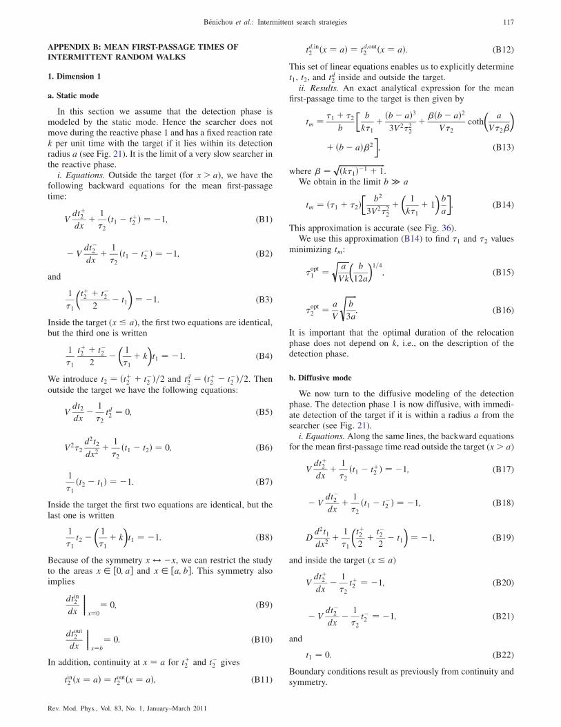
APPENDIX B: MEAN FIRST-PASSAGE TIMES OF

INTERMITTENT RANDOM WALKS

1. Dimension 1

a. Static mode

In this section we assume that the detection phase ismodeled by the static mode. Hence the searcher does notmove during the reactive phase 1 and has a fixed reaction ratek per unit time with the target if it lies within its detectionradius a (see Fig. 21). It is the limit of a very slow searcher inthe reactive phase.

i. Equations. Outside the target (for x > a), we have thefollowing backward equations for the mean first-passagetime:

Vdtþ2dx

þ 1

�2ðt1 � tþ2 Þ ¼ �1; (B1)

� Vdt�2dx

þ 1

�2ðt1 � t�2 Þ ¼ �1; (B2)

and

1

�1

�tþ2 þ t�2

2� t1

�¼ �1: (B3)

Inside the target (x � a), the first two equations are identical,but the third one is written

1

�1

tþ2 þ t�22

��1

�1þ k

�t1 ¼ �1: (B4)

We introduce t2 ¼ ðtþ2 þ t�2 Þ=2 and td2 ¼ ðtþ2 � t�2 Þ=2. Thenoutside the target we have the following equations:

Vdt2dx

� 1

�2td2 ¼ 0; (B5)

V2�2d2t2dx2

þ 1

�2ðt1 � t2Þ ¼ 0; (B6)

1

�1ðt2 � t1Þ ¼ �1: (B7)

Inside the target the first two equations are identical, but thelast one is written

1

�1t2 �

�1

�1þ k

�t1 ¼ �1: (B8)

Because of the symmetry x $ �x, we can restrict the studyto the areas x 2 ½0; a� and x 2 ½a; b�. This symmetry alsoimplies

dtin2dx

��x¼0¼ 0; (B9)

dtout2

dx

��x¼b¼ 0: (B10)

In addition, continuity at x ¼ a for tþ2 and t�2 gives

tin2 ðx ¼ aÞ ¼ tout2 ðx ¼ aÞ; (B11)

td;in2 ðx ¼ aÞ ¼ td;out2 ðx ¼ aÞ: (B12)

This set of linear equations enables us to explicitly determinet1, t2, and td2 inside and outside the target.

ii. Results. An exact analytical expression for the meanfirst-passage time to the target is then given by

tm ¼ �1 þ �2b

�b

k�1þ ðb� aÞ3

3V2�22þ�ðb� aÞ2

V�2coth

�a

V�2�

�

þ ðb� aÞ�2

�; (B13)

where � ¼ ffiffiffiffiffiffiffiffiffiffiffiffiffiffiffiffiffiffiffiffiffiffiffiffiffiðk�1Þ�1 þ 1p

.We obtain in the limit b � a

tm ¼ ð�1 þ �2Þ�

b2

3V2�22þ

�1

k�1þ 1

�b

a

�: (B14)

This approximation is accurate (see Fig. 36).We use this approximation (B14) to find �1 and �2 values

minimizing tm:

�opt1 ¼

ffiffiffiffiffiffia

Vk

r �b

12a

�1=4

; (B15)

�opt2 ¼ a

V

ffiffiffiffiffiffib

3a

s: (B16)

It is important that the optimal duration of the relocationphase does not depend on k, i.e., on the description of thedetection phase.

b. Diffusive mode

We now turn to the diffusive modeling of the detectionphase. The detection phase 1 is now diffusive, with immedi-ate detection of the target if it is within a radius a from thesearcher (see Fig. 21).

i. Equations. Along the same lines, the backward equationsfor the mean first-passage time read outside the target (x > a)

Vdtþ2dx

þ 1

�2ðt1 � tþ2 Þ ¼ �1; (B17)

� Vdt�2dx

þ 1

�2ðt1 � t�2 Þ ¼ �1; (B18)

Dd2t1dx2

þ 1

�1

�tþ22þ t�2

2� t1

�¼ �1; (B19)

and inside the target (x � a)

Vdtþ2dx

� 1

�2tþ2 ¼ �1; (B20)

� Vdt�2dx

� 1

�2t�2 ¼ �1; (B21)

and

t1 ¼ 0: (B22)

Boundary conditions result as previously from continuity andsymmetry.



ii. Results. Standard but lengthy calculations lead to anexact expression of the mean first-detection time of the targettm given by Loverdo et al. (2009b). Three regimes can beidentified.

(i) In the first regime (b < D=V) intermittence is notfavorable.

(ii) For b > D=V and bD2=a3V2 < 1 intermittence is fa-vorable. In the low-target-density limit (b � a), thefollowing approximation of the mean first-passagetime around its minimum can be obtained:

tm ¼ ð�1 þ �2Þb�

b

3V2�22þ 1ffiffiffiffiffiffiffiffiffi

D�1p

�: (B23)

This expression gives a good approximation of tm inthis regime, in particular, around the optimum (seeFig. 37). The simplified tm expression (B23) is mini-mized for

�opt1 ¼ 1

2

ffiffiffiffiffiffiffiffiffiffiffiffi2b2D

9V4

3

s; (B24)

�opt2 ¼

ffiffiffiffiffiffiffiffiffiffiffiffi2b2D

9V4

3

s; (B25)

toptm ’

ffiffiffiffiffiffiffiffiffiffiffiffiffiffiffiffi35

24b4

DV2

3

s: (B26)

This compares to the case without intermittenceaccording to

gainopt ¼ tdiff

toptm

’ffiffiffiffiffi24

383

s �bV

D

�2=3 ’ 0:13

�bV

D

�2=3

:

(B27)

(iii) For b > D=V and 1 � bD2=a3V2 intermittence isfavorable.

In this regime, the mean search time is given by

tm ’ b

að�1 þ �2Þ

�a

aþ ffiffiffiffiffiffiffiffiffiD�1

p þ ab

3V2�22

�: (B28)

This expression gives a good approximation of tm, at leastaround the optimum (see Fig. 38), which is characterized by

�opt1 ¼ Db

48V2a; (B29)

�opt2 ¼ a

V

ffiffiffiffiffiffib

3a

s; (B30)

toptm ’ 2a

Vffiffiffi3

p�b

a

�3=2

; (B31)

FIG. 36. Static mode in one dimension. Exact expression of tm (B13) (lines) compared to the approximation of tm (B14) (symbols), both

rescaled by toptm . �

opt1 from (B15), �

opt2 from (B16). V ¼ 1, k ¼ 1. b=a ¼ 10 (h), b=a ¼ 100 ( � ), and b=a ¼ 1000 (þ ).



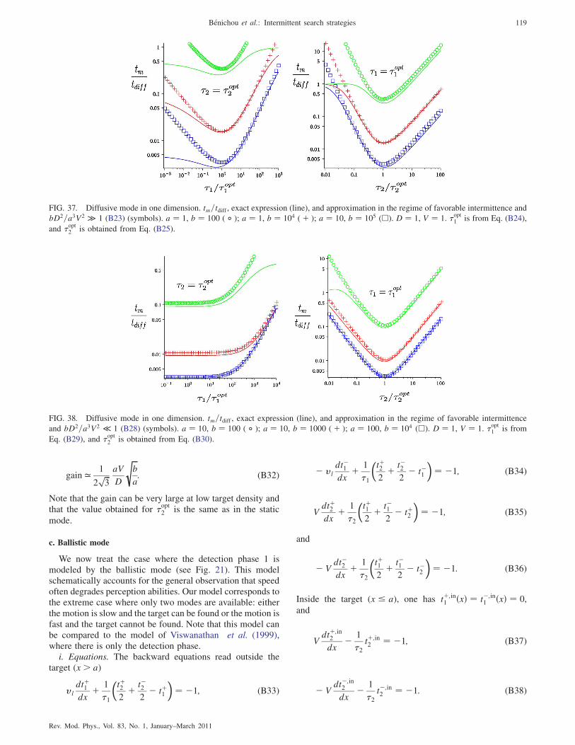
gain ’ 1

2ffiffiffi3

p aV

D

ffiffiffib

a

s: (B32)

Note that the gain can be very large at low target density andthat the value obtained for �

opt2 is the same as in the static

mode.

c. Ballistic mode

We now treat the case where the detection phase 1 ismodeled by the ballistic mode (see Fig. 21). This modelschematically accounts for the general observation that speedoften degrades perception abilities. Our model corresponds tothe extreme case where only two modes are available: eitherthe motion is slow and the target can be found or the motion isfast and the target cannot be found. Note that this model canbe compared to the model of Viswanathan et al. (1999),where there is only the detection phase.

i. Equations. The backward equations read outside thetarget (x > a)

vl

dtþ1dx

þ 1

�1

�tþ22þ t�2

2� tþ1

�¼ �1; (B33)

� vl

dt�1dx

þ 1

�1

�tþ22þ t�2

2� t�1

�¼ �1; (B34)

Vdtþ2dx

þ 1

�2

�tþ12þ t�1

2� tþ2

�¼ �1; (B35)

and

� Vdt�2dx

þ 1

�2

�tþ12þ t�1

2� t�2

�¼ �1: (B36)

Inside the target (x � a), one has tþ;in1 ðxÞ ¼ t�;in

1 ðxÞ ¼ 0,and

Vdtþ;in

2

dx� 1

�2tþ;in2 ¼ �1; (B37)

� Vdt�;in

2

dx� 1

�2t�;in2 ¼ �1: (B38)

FIG. 37. Diffusive mode in one dimension. tm=tdiff , exact expression (line), and approximation in the regime of favorable intermittence and

bD2=a3V2 � 1 (B23) (symbols). a ¼ 1, b ¼ 100 ( � ); a ¼ 1, b ¼ 104 (þ ); a ¼ 10, b ¼ 105 (h). D ¼ 1, V ¼ 1. �opt1 is from Eq. (B24),

and �opt2 is obtained from Eq. (B25).

FIG. 38. Diffusive mode in one dimension. tm=tdiff , exact expression (line), and approximation in the regime of favorable intermittence

and bD2=a3V2 � 1 (B28) (symbols). a ¼ 10, b ¼ 100 ( � ); a ¼ 10, b ¼ 1000 (þ ); a ¼ 100, b ¼ 104 (h). D ¼ 1, V ¼ 1. �opt1 is from

Eq. (B29), and �opt2 is obtained from Eq. (B30).



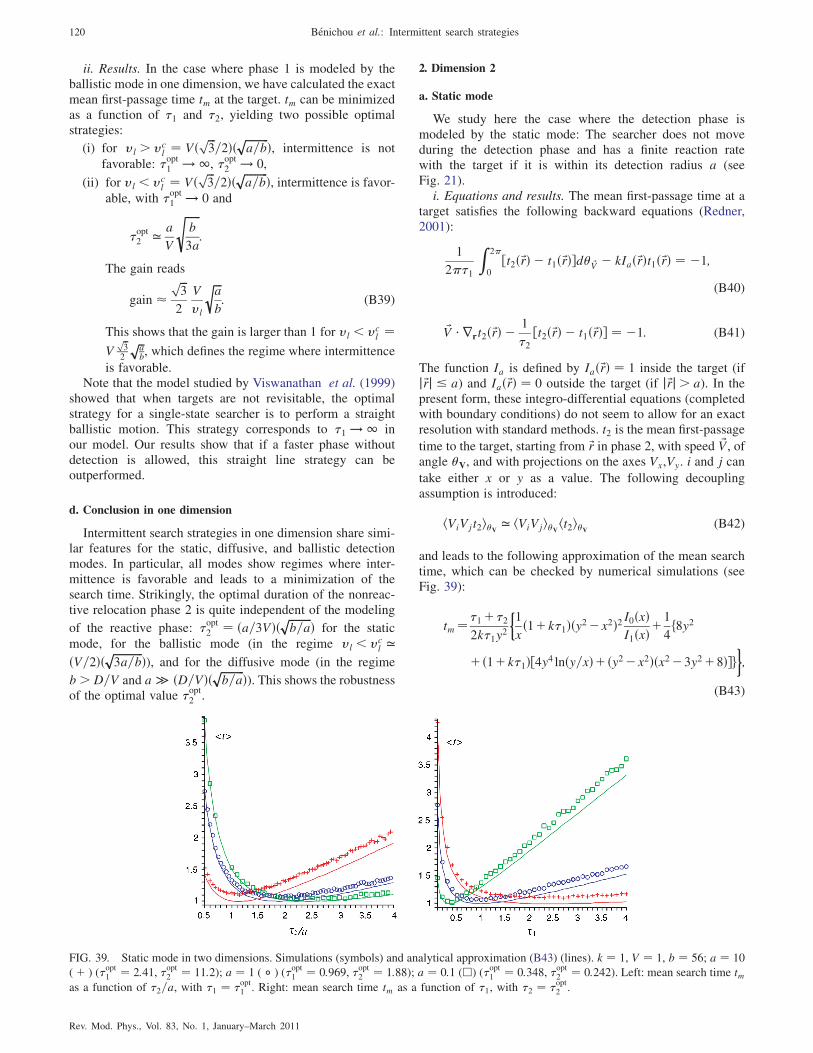
ii. Results. In the case where phase 1 is modeled by theballistic mode in one dimension, we have calculated the exactmean first-passage time tm at the target. tm can be minimizedas a function of �1 and �2, yielding two possible optimalstrategies:

(i) for vl > vcl ¼ Vð ffiffiffi

3p

=2Þð ffiffiffiffiffiffiffiffiffia=b

p Þ, intermittence is not

favorable: �opt1 ! 1, �

opt2 ! 0,

(ii) for vl < vcl ¼ Vð ffiffiffi

3p

=2Þð ffiffiffiffiffiffiffiffiffia=b

p Þ, intermittence is favor-

able, with �opt1 ! 0 and

�opt2 ’ a

V

ffiffiffiffiffiffib

3a

s:

The gain reads

gain �ffiffiffi3

p2

V

vl

ffiffiffia

b

r: (B39)

This shows that the gain is larger than 1 for vl < vcl ¼

Vffiffi3

p2

ffiffiab

p, which defines the regime where intermittence

is favorable.Note that the model studied by Viswanathan et al. (1999)

showed that when targets are not revisitable, the optimalstrategy for a single-state searcher is to perform a straightballistic motion. This strategy corresponds to �1 ! 1 inour model. Our results show that if a faster phase withoutdetection is allowed, this straight line strategy can beoutperformed.

d. Conclusion in one dimension

Intermittent search strategies in one dimension share simi-lar features for the static, diffusive, and ballistic detectionmodes. In particular, all modes show regimes where inter-mittence is favorable and leads to a minimization of thesearch time. Strikingly, the optimal duration of the nonreac-tive relocation phase 2 is quite independent of the modeling

of the reactive phase: �opt2 ¼ ða=3VÞð ffiffiffiffiffiffiffiffiffi

b=ap Þ for the static

mode, for the ballistic mode (in the regime vl < vcl ’

ðV=2Þð ffiffiffiffiffiffiffiffiffiffiffi3a=b

p Þ), and for the diffusive mode (in the regime

b > D=V and a � ðD=VÞð ffiffiffiffiffiffiffiffiffib=a

p Þ). This shows the robustnessof the optimal value �

opt2 .

2. Dimension 2

a. Static mode

We study here the case where the detection phase ismodeled by the static mode: The searcher does not moveduring the detection phase and has a finite reaction ratewith the target if it is within its detection radius a (seeFig. 21).

i. Equations and results. The mean first-passage time at atarget satisfies the following backward equations (Redner,2001):

1

2��1

Z 2�

0½t2ð~rÞ � t1ð~rÞ�d� ~V � kIað~rÞt1ð~rÞ ¼ �1;

(B40)

~V � rrt2ð~rÞ � 1

�2½t2ð~rÞ � t1ð~rÞ� ¼ �1: (B41)

The function Ia is defined by Iað~rÞ ¼ 1 inside the target (ifj ~rj � a) and Iað~rÞ ¼ 0 outside the target (if j~rj> a). In thepresent form, these integro-differential equations (completedwith boundary conditions) do not seem to allow for an exactresolution with standard methods. t2 is the mean first-passage

time to the target, starting from ~r in phase 2, with speed ~V, ofangle �V, and with projections on the axes Vx,Vy. i and j can

take either x or y as a value. The following decouplingassumption is introduced:

hViVjt2i�V ’ hViVji�V ht2i�V (B42)

and leads to the following approximation of the mean searchtime, which can be checked by numerical simulations (seeFig. 39):

tm¼�1þ�22k�1y

2

�1

xð1þk�1Þðy2�x2Þ2 I0ðxÞ

I1ðxÞþ1

4f8y2

þð1þk�1Þ½4y4 lnðy=xÞþðy2�x2Þðx2�3y2þ8Þ�g�;

(B43)

FIG. 39. Static mode in two dimensions. Simulations (symbols) and analytical approximation (B43) (lines). k ¼ 1, V ¼ 1, b ¼ 56; a ¼ 10(þ ) (�opt1 ¼ 2:41, �opt2 ¼ 11:2); a ¼ 1 ( � ) (�opt1 ¼ 0:969, �opt2 ¼ 1:88); a ¼ 0:1 (h) (�opt1 ¼ 0:348, �opt2 ¼ 0:242). Left: mean search time tmas a function of �2=a, with �1 ¼ �opt1 . Right: mean search time tm as a function of �1, with �2 ¼ �opt2 .



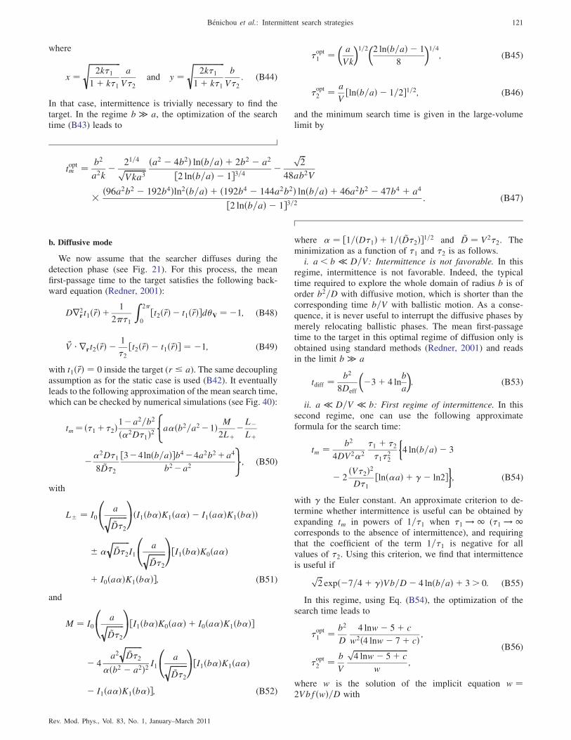
where

x ¼ffiffiffiffiffiffiffiffiffiffiffiffiffiffiffiffiffi2k�1

1þ k�1

sa

V�2and y ¼

ffiffiffiffiffiffiffiffiffiffiffiffiffiffiffiffiffi2k�1

1þ k�1

sb

V�2: (B44)

In that case, intermittence is trivially necessary to find thetarget. In the regime b � a, the optimization of the searchtime (B43) leads to

�opt1 ¼

�a

Vk

�1=2


8

�1=4

; (B45)

�opt2 ¼ a

V½lnðb=aÞ � 1=2�1=2; (B46)

and the minimum search time is given in the large-volumelimit by

toptm ¼ b2

a2k� 21=4ffiffiffiffiffiffiffiffiffiffiffi

Vka3p ða2 � 4b2Þ lnðb=aÞ þ 2b2 � a2

½2 lnðb=aÞ � 1�3=4 �ffiffiffi2

p48ab2V

ð96a2b2 � 192b4Þln2ðb=aÞ þ ð192b4 � 144a2b2Þ lnðb=aÞ þ 46a2b2 � 47b4 þ a4

½2 lnðb=aÞ � 1�3=2 : (B47)

b. Diffusive mode

We now assume that the searcher diffuses during thedetection phase (see Fig. 21). For this process, the meanfirst-passage time to the target satisfies the following back-ward equation (Redner, 2001):

Dr2rt1ð~rÞ þ 1

2��1

Z 2�

0½t2ð~rÞ � t1ð~rÞ�d�V ¼�1; (B48)

~V � rrt2ð~rÞ � 1

�2½t2ð~rÞ � t1ð~rÞ� ¼ �1; (B49)

with t1ð~rÞ ¼ 0 inside the target (r � a). The same decouplingassumption as for the static case is used (B42). It eventuallyleads to the following approximation of the mean search time,which can be checked by numerical simulations (see Fig. 40):

tm¼ð�1þ�2Þ1�a2=b2

ð�2D�1Þ28<:a�ðb2=a2�1Þ M

2Lþ�L�Lþ

��2D�1

8 ~D�2

½3�4lnðb=aÞ�b4�4a2b2þa4

b2�a2

9=;; (B50)

with

L ¼ I0

0@ affiffiffiffiffiffiffiffiffi

~D�2

q1AðI1ðb�ÞK1ða�Þ � I1ða�ÞK1ðb�ÞÞ

�ffiffiffiffiffiffiffiffiffi~D�2

qI1


~D�2

q1A½I1ðb�ÞK0ða�Þ

þ I0ða�ÞK1ðb�Þ�; (B51)

and

M ¼ I0


~D�2

q1A½I1ðb�ÞK0ða�Þ þ I0ða�ÞK1ðb�Þ�

� 4a2

ffiffiffiffiffiffiffiffiffi~D�2

q�ðb2 � a2Þ2 I1


~D�2

q1A½I1ðb�ÞK1ða�Þ

� I1ða�ÞK1ðb�Þ�; (B52)

where � ¼ ½1=ðD�1Þ þ 1=ð ~D�2Þ�1=2 and ~D ¼ V2�2. Theminimization as a function of �1 and �2 is as follows.

i. a < b � D=V: Intermittence is not favorable. In thisregime, intermittence is not favorable. Indeed, the typicaltime required to explore the whole domain of radius b is oforder b2=D with diffusive motion, which is shorter than thecorresponding time b=V with ballistic motion. As a conse-quence, it is never useful to interrupt the diffusive phases bymerely relocating ballistic phases. The mean first-passagetime to the target in this optimal regime of diffusion only isobtained using standard methods (Redner, 2001) and readsin the limit b � a

tdiff ¼ b2

8Deff

��3þ 4 ln

b

a

�: (B53)

ii. a � D=V � b: First regime of intermittence. In thissecond regime, one can use the following approximateformula for the search time:

tm ¼ b2

4DV2�2

�1 þ �2�1�

22


� 2ðV�2Þ2D�1

½lnð�aÞ þ � ln2��; (B54)

with the Euler constant. An approximate criterion to de-termine whether intermittence is useful can be obtained byexpanding tm in powers of 1=�1 when �1 ! 1 (�1 ! 1corresponds to the absence of intermittence), and requiringthat the coefficient of the term 1=�1 is negative for allvalues of �2. Using this criterion, we find that intermittenceis useful ifffiffiffi

2p

expð�7=4þ ÞVb=D� 4 lnðb=aÞ þ 3> 0: (B55)

In this regime, using Eq. (B54), the optimization of thesearch time leads to

�opt1 ¼ b2

D

4 lnw� 5þ c

w2ð4 lnw� 7þ cÞ ;

�opt2 ¼ b

V

ffiffiffiffiffiffiffiffiffiffiffiffiffiffiffiffiffiffiffiffiffiffiffiffiffiffiffiffiffi4 lnw� 5þ c

pw

;

(B56)

where w is the solution of the implicit equation w ¼2VbfðwÞ=D with



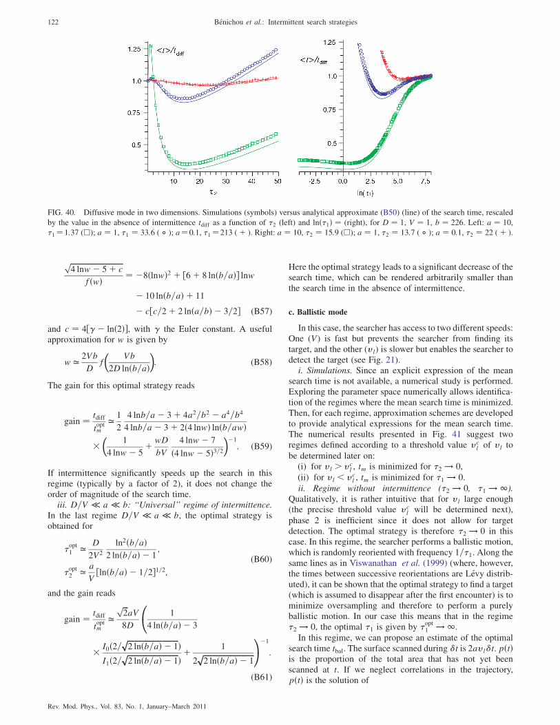
ffiffiffiffiffiffiffiffiffiffiffiffiffiffiffiffiffiffiffiffiffiffiffiffiffiffiffiffiffi4 lnw� 5þ c

pfðwÞ ¼ �8ðlnwÞ2 þ ½6þ 8 lnðb=aÞ� lnw

� 10 lnðb=aÞ þ 11

� c½c=2þ 2 lnða=bÞ � 3=2� (B57)

and c ¼ 4½ � lnð2Þ�, with the Euler constant. A usefulapproximation for w is given by

w ’ 2Vb

Df

�Vb

2D lnðb=aÞ�: (B58)

The gain for this optimal strategy reads

gain ¼ tdiff

toptm

’ 1

2

4 lnb=a� 3þ 4a2=b2 � a4=b4

4 lnb=a� 3þ 2ð4 lnwÞ lnðb=awÞ

�1

4 lnw� 5þ wD

bV

4 lnw� 7

ð4 lnw� 5Þ3=2��1

: (B59)

If intermittence significantly speeds up the search in thisregime (typically by a factor of 2), it does not change theorder of magnitude of the search time.

iii. D=V � a � b: ‘‘Universal’’ regime of intermittence.In the last regime D=V � a � b, the optimal strategy isobtained for

�opt1 ’ D

2V2

ln2ðb=aÞ2 lnðb=aÞ � 1

;

�opt2 ’ a

V½lnðb=aÞ � 1=2�1=2;

(B60)

and the gain reads

gain ¼ tdiff

toptm

’ffiffiffi2

paV

8D

0@ 1

4 lnðb=aÞ � 3

I0ð2=ffiffiffiffiffiffiffiffiffiffiffiffiffiffiffiffiffiffiffiffiffiffiffiffiffiffiffiffi2 lnðb=aÞ � 1

p ÞI1ð2=

ffiffiffiffiffiffiffiffiffiffiffiffiffiffiffiffiffiffiffiffiffiffiffiffiffiffiffiffi2 lnðb=aÞ � 1

p Þþ 1

2ffiffiffiffiffiffiffiffiffiffiffiffiffiffiffiffiffiffiffiffiffiffiffiffiffiffiffiffi2 lnðb=aÞ � 1

p1A�1

:

(B61)

Here the optimal strategy leads to a significant decrease of thesearch time, which can be rendered arbitrarily smaller thanthe search time in the absence of intermittence.

c. Ballistic mode

In this case, the searcher has access to two different speeds:One (V) is fast but prevents the searcher from finding itstarget, and the other (vl) is slower but enables the searcher todetect the target (see Fig. 21).

i. Simulations. Since an explicit expression of the meansearch time is not available, a numerical study is performed.Exploring the parameter space numerically allows identifica-tion of the regimes where the mean search time is minimized.Then, for each regime, approximation schemes are developedto provide analytical expressions for the mean search time.The numerical results presented in Fig. 41 suggest tworegimes defined according to a threshold value vc

l of vl to

be determined later on:(i) for vl > vc

l , tm is minimized for �2 ! 0,(ii) for vl < vc

l , tm is minimized for �1 ! 0.ii. Regime without intermittence (�2 ! 0, �1 ! 1).

Qualitatively, it is rather intuitive that for vl large enough(the precise threshold value vc

l will be determined next),

phase 2 is inefficient since it does not allow for targetdetection. The optimal strategy is therefore �2 ! 0 in thiscase. In this regime, the searcher performs a ballistic motion,which is randomly reoriented with frequency 1=�1. Along thesame lines as in Viswanathan et al. (1999) (where, however,the times between successive reorientations are Levy distrib-uted), it can be shown that the optimal strategy to find a target(which is assumed to disappear after the first encounter) is tominimize oversampling and therefore to perform a purelyballistic motion. In our case this means that in the regime�2 ! 0, the optimal �1 is given by �

opt1 ! 1.

In this regime, we can propose an estimate of the optimalsearch time tbal. The surface scanned during �t is 2avl�t. pðtÞis the proportion of the total area that has not yet beenscanned at t. If we neglect correlations in the trajectory,pðtÞ is the solution of

FIG. 40. Diffusive mode in two dimensions. Simulations (symbols) versus analytical approximate (B50) (line) of the search time, rescaled

by the value in the absence of intermittence tdiff as a function of �2 (left) and lnð�1Þ ¼ (right), for D ¼ 1, V ¼ 1, b ¼ 226. Left: a ¼ 10,�1¼1:37 (h); a ¼ 1, �1 ¼ 33:6 ( � ); a¼0:1, �1¼213 (þ ). Right: a ¼ 10, �2 ¼ 15:9 (h); a ¼ 1, �2 ¼ 13:7 ( � ); a ¼ 0:1, �2 ¼ 22 (þ ).



dp

dt¼ � 2avlpðtÞ

�b2: (B62)

Then, given that pðt ¼ 0Þ ¼ 1, we obtain

pðtÞ ¼ exp

�� 2avl

�b2

�; (B63)

and the mean first-passage time to the target in these con-ditions is

tbal ¼ �Z 1

0tdp

dtdt ¼ �b2

2avl

: (B64)

This expression yields good agreement with numerical simu-lations. Note, in particular, that tbal / 1=vl.

iii. Regime with intermittence (�1 ! 0). In this regimewhere vl < vc

l , the numerical study shows that the search

time is minimized for �1 ! 0 (see Fig. 41). We determinehere the optimal value of �2 in this regime. To proceed, weapproximate the problem by the case of a diffusive modepreviously studied (B50), with an effective diffusion coeffi-cient

D ¼ v2l �12

: (B65)

This approximation is very satisfactory in the regime �1 ! 0(see Fig. 41).

We can then use the results of the previous section for thediffusive mode in the �1 ! 0 regime and obtain

tm ¼ �2

�1� a2

b2

��1� 1

4

½3þ 4 lnða=bÞ�b4 � 4a2b2 þ a4

�22V2ðb2 � a2Þ

þ a

V�2ffiffiffi2

p�b2

a2� 1

�I0ða

ffiffiffi2

p=�2VÞ

I1ðaffiffiffi2

p=�2VÞ

�: (B66)

The calculation of �opt2 minimizing tm then gives

�opt2 ¼ a

V

ffiffiffiffiffiffiffiffiffiffiffiffiffiffiffiffiffiffiffiffiffiln

�b

a

�� 1

2

s: (B67)

Finally the gain reads

gain ¼ tbal

toptm

’ �V

4vl

�ln

�b

a

��0:5: (B68)

iv. Determination of vcl . Note that an estimate of vc

l can be

obtained from (B68) as the value of vl for which gain ¼ 1:

vcl ’

�V

4

�ln

�b

a

��0:5 / Vffiffiffiffiffiffiffiffiffiffiffiffiffiffiffiffilnðb=aÞp : (B69)

It is noteworthy that intermittence becomes less favorablewith increasing b. This effect is similar to the one-dimensional case, even though it is less important here. Itcan be understood as follows: at very large scales the inter-mittent trajectory is reoriented many times and thereforescales as diffusion, which is less favorable than the non-intermittent ballistic motion.

d. Conclusion in dimension 2

Remarkably, for the three different modes of detection(static, diffusive, and ballistic), we find a regime whereintermittence minimizes the search time for one and the

same �opt2 , given by �

opt2 ¼ ða=VÞ

ffiffiffiffiffiffiffiffiffiffiffiffiffiffiffiffiffiffiffiffiffiffiffiffilnðb=aÞ � 1

2

q. As in one

dimension, this indicates that optimal intermittent strategiesare robust and widely independent of the details of thedescription of the detection mechanism.

3. Dimension 3

a. Static mode

We study in this section the case where the detection phaseis modeled by the static mode, for which the searcher does notmove during the detection phase, and has a finite reaction ratewith the target if it is within a detection radius a (see Fig. 21).

i. Equations. Denoting by t1ðrÞ the mean first-passage timeto the target starting from a distance r from the target inphase 1 (detection phase), and by t2;�;�ðrÞ the mean first-

passage time to the target starting from a distance r from the

FIG. 41. Ballistic mode in two dimensions. lnðtmÞ as a function of lnð�2Þ. Simulations (symbols), diffusive-diffusive approximation (B50)

with (B65) (lines), �1 ! 0 limit (B66) (line), �1 ! 1 (no intermittence) (B64) (dotted line). b ¼ 30, a ¼ 1, V ¼ 1. �1 ¼ 0 ( ? ), �1 ¼ 0:17( � ), �1 ¼ 0:92 (�), �1 ¼ 5:0 ( ), �1 ¼ 28 ( � ), �1 ¼ 150 (þ ), �1 ¼ 820 (h).



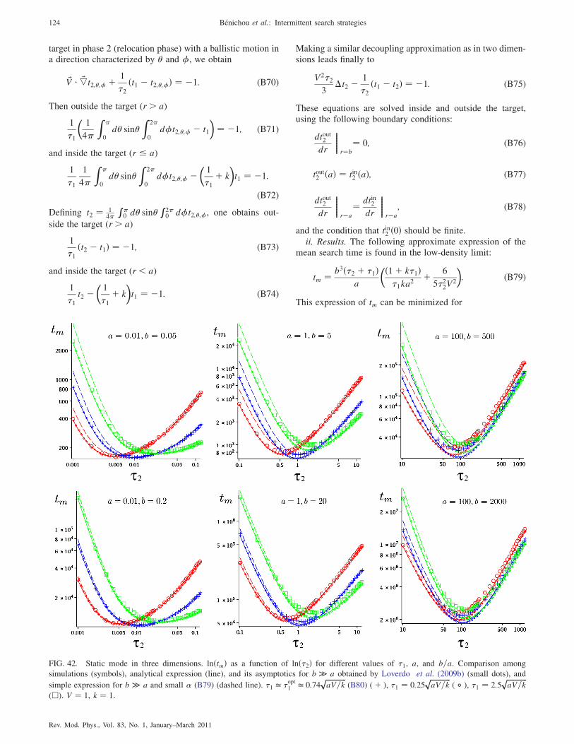
target in phase 2 (relocation phase) with a ballistic motion ina direction characterized by � and �, we obtain

~V � ~5t2;�;� þ 1

�2ðt1 � t2;�;�Þ ¼ �1: (B70)

Then outside the target (r > a)

1

�1

�1

4�

Z �

0d� sin�

Z 2�

0d�t2;�;� � t1

�¼ �1; (B71)

and inside the target (r � a)

1

�1

1

4�

Z �

0d� sin�

Z 2�

0d�t2;�;� �

�1

�1þ k

�t1 ¼ �1:

(B72)

Defining t2 ¼ 14�

R�0 d� sin�

R2�0 d�t2;�;�, one obtains out-

side the target (r > a)

1

�1ðt2 � t1Þ ¼ �1; (B73)

and inside the target (r < a)

1

�1t2 �

�1

�1þ k

�t1 ¼ �1: (B74)

Making a similar decoupling approximation as in two dimen-sions leads finally to

V2�23

�t2 � 1

�2ðt1 � t2Þ ¼ �1: (B75)

These equations are solved inside and outside the target,using the following boundary conditions:

dtout2

dr

��r¼b¼ 0; (B76)

tout2 ðaÞ ¼ tin2 ðaÞ; (B77)

dtout2

dr

��r¼a¼ dtin2

dr

��r¼a; (B78)

and the condition that tin2 ð0Þ should be finite.

ii. Results. The following approximate expression of themean search time is found in the low-density limit:

tm ¼ b3ð�2 þ �1Þa

�ð1þ k�1Þ�1ka

2þ 6

5�22V2

�: (B79)

This expression of tm can be minimized for

FIG. 42. Static mode in three dimensions. lnðtmÞ as a function of lnð�2Þ for different values of �1, a, and b=a. Comparison among

simulations (symbols), analytical expression (line), and its asymptotics for b � a obtained by Loverdo et al. (2009b) (small dots), and

simple expression for b � a and small � (B79) (dashed line). �1 ’ �opt1 ’ 0:74

ffiffiffiffiffiffiffiffiffiffiffiffiaV=k

p(B80) (þ ), �1 ¼ 0:25


p( � ), �1 ¼ 2:5


p(h). V ¼ 1, k ¼ 1.



�opt1 ¼

�3

10

�1=4

ffiffiffiffiffiffia

Vk

r; (B80)

�opt2 ¼ ffiffiffiffiffiffiffi

1:2p a

V; (B81)

and the minimum mean search time finally reads

toptm ¼ 1ffiffiffi

5p 1

k

b3

a3

� ffiffiffiffiffiffiak

V

s241=4 þ 51=4

�2: (B82)

Data obtained by numerical simulations (Fig. 42) are ingood agreement with the analytical expression (B79) exceptfor small �2 or small b, where a refined analytical expressioncan be obtained [see Loverdo et al. (2009b)]. In particular,the position of the minimum is very well approximated, andthe error on the value of the mean search time at the minimumis close to 10%.

With the static detection mode, intermittence is alwaysfavorable and leads to a single optimal intermittent strategy.As in one and two dimensions, the optimal duration of therelocation phase does not depend on k, i.e., on the descriptionof the detection phase. In addition, this optimal strategy doesnot depend on the typical distance between targets b.

Note that for the static mode in the three cases studied

(1, 2, and 3 dimensions), we have �opt1 ¼

ffiffiffiffiffiffiffiffiffiffiffiffiffiffiffiffiffiffiffi�opt2 =ð2kÞ

q. This

relation between the optimal durations of the two phases isindependent of the dimension.

b. Diffusive mode

We now study the case where the detection phase ismodeled by a diffusive mode. During the detection phase,the searcher diffuses and detects the target as soon as itsrespective distance is less than a (see Fig. 21).

i. Equations. Outside the target (r > a), one has

~V � ~5t2;�;� þ 1

�2ðt1 � t2;�;�Þ ¼ �1; (B83)

D�t1 þ 1

�1

�1

4�

Z �

0d� sin�

Z 2�

0d�t2;�;� � t1

�¼ �1;

(B84)


~V � ~rt2;�;� � 1

�2t2;�;� ¼ �1; (B85)

t1 ¼ 0: (B86)

With t2 ¼ 14�

R�0 d� sin�

R2�0 d�t2;�;�, one obtains outside

the target (r > a)

D�tout1 þ 1

�1ðtout2 � tout1 Þ ¼ �1: (B87)

The decoupling approximation described previously thenyields outside the target

V2�23

�tout2 þ 1

�2ðtout1 � tout2 Þ ¼ �1; (B88)


V2�23

�tint2 � 1

�2tint2 ¼ �1: (B89)

These equations are completed by the following boundaryconditions:

dtout2

dr

��r¼b¼ 0; (B90)

tout2 ðaÞ ¼ tint2 ðaÞ; (B91)

dtout2

dr

��r¼a¼ dtint2

dr

��r¼a: (B92)

ii. Results in the general case. Through standardbut lengthy calculations the above system can be solvedand leads to an analytical approximation of tm [see Loverdoet al. (2009b)]. In the regime b � a and

bffiffiffiffiffiffiffiffiffiffiffiffiffiffiffiffiffiffiffiffiffiffiffiffiffiffiffiffiffiffiffiffiffiffiffiffiffiffiffiffiffiffið�1DÞ�1 þ 3ð�2vÞ�2

p � 1, one obtains

tm ¼ b3�42ð�1 þ �2Þ�1

tanhð�2aÞ þ �1=�2

�1�22�1Da½tanhð�2aÞ þ �1=�2� � tanhð�2aÞ

(B93)

with �1 ¼ffiffiffiffiffiffiffiffiffiffiffiffiffiffiffiffiffiffiffiffiffiffiffiffiffiffiffiffi�22V

2 þ 3�1Dq

=�2VffiffiffiffiffiffiffiffiffiD�1

pand �2 ¼

ffiffiffi3

p=V�2. It

can be shown that tm only weakly depends on �1, whichindicates that this variable will be less important than �2 inthe minimization of the search time. The relevant order ofmagnitude for �

opt1 can be evaluated by comparing the typical

diffusion length Ldiff ¼ffiffiffiffiffiffiffiffiffi6Dt

pand the typical ballistic length

Lbal ¼ Vt. An estimate of the optimal time �opt1 can be given

by the time scale for which those lengths are of the sameorder, which gives

�opt1 � 6D

V2: (B94)

In turn, the minimization of tm leads to

�opt2 ¼

ffiffiffi3

pa

Vx; (B95)

with x the solution of

2 tanhðxÞ � 2xþ x tanhðxÞ2 ¼ 0: (B96)

This finally yields

�opt2 ’ 1:078

a

V: (B97)

It is important that this approximate expression is very

close to the expression obtained for the static mode (�opt2 ¼

ð ffiffiffiffiffiffiffiffi6=5

p Þða=VÞ ’ 1:095ða=VÞ) (B81), and there is no depen-dence on the typical distance between targets b. The simpli-fied expression for the minimal tm can then be obtained as

toptm ¼ b3x2ffiffiffi

3p

a2V½x� tanhðxÞ��1 ’ 2:18

b3

a2V; (B98)

and the gain reads



gain ¼ tdiff

toptm

’ 0:15aV

D; (B99)

where the search time without intermittence is given bytdiff ’ b3=3Da for b � a (Redner, 2001).

There is a range of parameters for which intermittenceis favorable, as indicated by Fig. 43. Both the analyticalexpression for t

optm in the regimes without intermittence and

with intermittence (B98) scale as b3. However, the depen-dence on a is different. In the diffusive regime tm / a�1,whereas in the intermittent regime tm / a�2. This enablesus to define a critical ac, such that when a > ac, intermittenceis favorable: ac ’ 6:5D=V is the value for which the gain(B99) is 1.

c. Ballistic mode

We now discuss the last case, where the detection phase 1is modeled by a ballistic mode (see Fig. 21). Since an explicitanalytical determination of the search time seems out ofreach, a numerical exploration of the parameter space isneeded to identify the regimes where the search time canbe minimized. Approximation schemes are then developedin each regime to obtain analytical expressions [more detailsare given in Loverdo et al. (2009b)].

i. Numerical study. The numerical analysis performed byLoverdo et al. (2009b) puts forward two strategies minimiz-ing the search time, depending on a critical value vc

l to be

determined later on:(i) When vl > vc

l , �opt1 ! 1 and �

opt2 ! 0. In this regime

intermittence is not favorable.(ii) When vl < vc

l , �opt1 ! 0 and �

opt2 is finite. In this

regime the optimal strategy is intermittent.ii. Regime without intermittence (single-state ballistic

searcher): �2 ! 0. Following the same argument as in twodimensions, without intermittence the best strategy is ob-tained in the limit �1 ! 1 in order to minimize oversamplingof the search space. Following the derivation of (B64) [seeLoverdo et al. (2009b) for details], it is found that the searchtime reads

tbal ¼ 4b3

3a2vl

: (B100)

iii. Regime with intermittence. In the regime of favorableintermittence, the numerical study suggests that the beststrategy is realized for �1 ! 0. In this regime �1 ! 0, phase 1can be well approximated by diffusion with an effectivediffusion coefficient Deff ¼ v2

l �1=3. The analytical expres-

sion tm derived in (B93) can then be used and yields for�1 ¼ 0 and b � a

tm ¼ b3ffiffiffi3

pV2�22

24

ffiffiffi3

pa

V�2� tanh

0@

ffiffiffi3

pa

V�2

1A35�1

: (B101)

Then one finds straightforwardly that �opt2 ¼ ffiffiffi

3p

a=Vx, wherex is the solution of x tanhðxÞ2 þ 2 tanhðxÞ � 2x ¼ 0, that is,x ’ 1:606. Using this optimal value of �2 in the expressionof tm, one finally obtains

toptm ¼ 2ffiffiffi

3p x

tanhðxÞ2b3

a2V’ 2:18

b3

a2V: (B102)

These expressions show good agreement with numericalsimulations [see Loverdo et al. (2009b)].

iv. Discussion of the critical value vcl . The gain is given by

gain ¼ tbal

toptm

’ 0:61V

vl

: (B103)

As in two dimensions, it is trivial that vcl < V, and the critical

value vcl can be defined as the value of vl such that gain ¼ 1.

This yields

vcl ’ 0:6V: (B104)

Importantly, vcl depends on neither b nor a. Simulations are in

good agreement with this result, except for a small numericalshift.

FIG. 43. Diffusive mode in three dimensions. tm=tdiff as a function of �2 for different values of the ratio b=a (logarithmic scale). The full

analytical form given in Loverdo et al. (2009b) (plain lines) is plotted against the simplified expression (B93) (dashed lines), the simplified

expression with �1 ¼ 0 (dotted line), and numerical simulations (symbols) for the following values of the parameters (arbitrary units): a ¼ 1(h); a ¼ 5 ( ? ); a ¼ 7 ( � ); a ¼ 10 (þ ); a ¼ 14 ( ); a ¼ 20 (�). �1 ¼ 6 everywhere except for the small dots, V ¼ 1, D ¼ 1. tm=tdiffpresents a minimum only for a > ac ’ 4.



d. Conclusion in dimension 3

For the three possible modelings of the detection mode(static, diffusive, and ballistic) in three dimensions, thereis a regime where the optimal strategy is intermittent.Remarkably, and as was the case in one and two dimensions,the optimal time to spend in the fast nonreactive phase 2 isindependent of the modeling of the detection mode and reads�opt2 ’ 1:1a=V. Additionally, while the mean first-passage

time to the target scales as b3, the optimal values of thedurations of the two phases do not depend on the targetdensity a=b.

REFERENCES

Adam, G., and M. Delbruck, 1968, in Structural Chemistry and

Molecular Biology, edited by A. Rich and N. Davidson (Freeman,

San Francisco), pp. 198–215.

Ajdari, A., 1995, Europhys. Lett. 31, 69.

Alberts, B., 2002, Molecular Biology of the Cell (Garland,

New York).

Anderson, J. P., D.W. Stephens, and S. R. Dunbar, 1997, Behavioral

Ecology 8, 307.

Bakk, A., and R. Metzler, 2004, FEBS Lett. 563, 66.

Balkovsky, E., and B. I. Shraiman, 2002, Proc. Natl. Acad. Sci.

U.S.A. 99, 12589.

Bancaud, A., S. Huet, N. Daigle, J. Mozziconacci, J. Beaudouin,

and J. Ellenberg, 2009, EMBO J. 28, 3785.

Barabasi, A. L., and R. Albert, 1999, Science 286, 509.

Barbi, M., C. Place, V. Popkov, and M. Salerno, 2004, Phys. Rev. E

70, 041901.

Bartumeus, F., 2009, Oikos 118, 488.

Bartumeus, F., J. Catalan, U. L. Fulco, M. L. Lyra, and G.M.

Viswanathan, 2002, Phys. Rev. Lett. 88, 097901.

Bartumeus, F., and S. A. Levin, 2008, Proc. Natl. Acad. Sci. U.S.A.

105, 19072.

Bartumeus, F., F. Peters, S. Pueyo, C. Marrase, and J. Catalan, 2003,

Proc. Natl. Acad. Sci. U.S.A. 100, 12771.

Bell, W. J., 1991, Searching Behaviour: The Behavioural Ecology of

Finding Resources (Chapman and Hall, London).

Ben-Avraham, D., and S. Havlin, 2000, Diffusion and Reaction in

Fractals and Disorders Systems (Cambridge University Press,

Cambridge, England).

Benhamou, S., 1992, J. Theor. Biol. 159, 67.

Benhamou, S., 2007, Ecology 88, 1962.

Benichou, O., C. Chevalier, J. Klafter, B. Meyer, and R. Voituriez,

2010, Nature Chem. 2, 472.

Benichou, O., C. Chevalier, B. Meyer, and R. Voituriez, 2011, Phys.

Rev. Lett. 106, 038102.

Benichou, O., M. Coppey, M. Moreau, P.-H. Suet, and R. Voituriez,

2005a, Europhys. Lett. 70, 42.


2005b, Phys. Rev. Lett. 94, 198101.


2005c, J. Phys. Condens. Matter 17, S4275.


2005d, Physica (Amsterdam) 356A, 151.

Benichou, O., M. Coppey, M. Moreau, and R. Voituriez, 2006a,

Europhys. Lett. 75, 349.

Benichou, O., D. Grebenkov, P. Levitz, C. Loverdo, and R.

Voituriez, 2010, Phys. Rev. Lett. 105, 150606.

Benichou, O., D. Grebenkov, P. Levitz, C. Loverdo, and R.

Voituriez, 2011, J. Stat. Phys. 142, 657.

Benichou, O., Y. Kafri, M. Sheinman, and R. Voituriez, 2009, Phys.

Rev. Lett. 103, 138102.

Benichou, O., C. Loverdo, M. Moreau, and R. Voituriez, 2006b,

Phys. Rev. E 74, 020102.

Benichou, O., C. Loverdo, M. Moreau, and R. Voituriez, 2007,

J. Phys. Condens. Matter 19, 065141.

Benichou, O., C. Loverdo, M. Moreau, and R. Voituriez, 2008a,

Phys. Chem. Chem. Phys. 10, 7059.

Benichou, O., C. Loverdo, and R. Voituriez, 2008b, Europhys. Lett.

84, 38003.

Benichou, O., B. Meyer, V. Tejedor, and R. Voituriez, 2008, Phys.

Rev. Lett. 101, 130601.

Benichou, O., and R. Voituriez, 2008, Phys. Rev. Lett. 100,

168105.

Benichou, O., and R. Voituriez, 2009, J. Chem. Phys. 131, 181104.

Berg, H. C., 2004, E. Coli in Motion (Springer, New York).

Berg, O.G., and C. Blomberg, 1976, Biophys. Chem. 4, 367.

Berg, O.G., R. B. Winter, and P. H. Von Hippel, 1981, Biochemistry

20, 6929.

Blanco, S., and R. Fournier, 2003, Europhys. Lett. 61, 168.

Block, S.M., C. L. Asbury, J.W. Shaevitz, and M. J. Lang, 2003,

Proc. Natl. Acad. Sci. U.S.A. 100, 2351.

Bonnet, I., A. Biebricher, P.-L. Porte, C. Loverdo, O. Benichou, R.

Voituriez, C. Escude, W. Wende, A. Pingoud, and P. Desbiolles,

2008, Nucleic Acids Res. 36, 4118.

Boyer, D., G. Ramos-Fernandez, O. Miramontes, J. L. Mateos, G.

Cocho, H. Larralde, H. Ramos, and F. Rojas, 2006, Proc. R. Soc.

B 273, 1743.

Bressloff, P., and J. Newby, 2009, New J. Phys. 11, 023033.

Bunde, A., and S. Havlin, 1991, Fractals and Disordered Systems

(Springer, Berlin).

Caspi, A., R. Granek, and M. Elbaum, 2000, Phys. Rev. Lett. 85,

5655.

Caspi, A., R. Granek, and M. Elbaum, 2002, Phys. Rev. E 66,

011916.

Champagne, L., R. G. Carl, and R. Hill, 2003, Proceedings of The

2003 Winter Simulation Conference 1–2, p. 991, http://ieeexplor-

e.ieee.org/xpls/abs_all.jsp?arnumber=1261521&tag=1.

Charnov, E. L., 1976, Theor. Popul. Biol. 9, 129.

Chechkin, A.V., M. Hofmann, and I. V. Sokolov, 2009, Phys. Rev. E

80, 031112.

Chechkin, A.V., I.M. Zaid, M.A. Lomholt, I.M. Sokolov, and R.

Metzler, 2009, Phys. Rev. E 79, 040105.

Condamin, S., O. Benichou, and J. Klafter, 2007a, Phys. Rev. Lett.

98, 250602.

Condamin, S., O. Benichou, and M. Moreau, 2005a, Phys. Rev. E

72, 016127.

Condamin, S., O. Benichou, and M. Moreau, 2005b, Phys. Rev.

Lett. 95, 260601.

Condamin, S., O. Benichou, V. Tejedor, R. Voituriez, and J. Klafter,

2007b, Nature (London) 450, 77.

Condamin, S., V. Tejedor, and O. Benichou, 2007c, Phys. Rev. E 76,

050102.

Condamin, S., V. Tejedor, R. Voituriez, O. Benichou, and J. Klafter,

2008, Proc. Natl. Acad. Sci. U.S.A. 105, 5675.

Coppey, M., O. Benichou, R. Voituriez, and M. Moreau, 2004,

Biophys. J. 87, 1640.

Dahirel, V., F. Paillusson, M. Jardat, M. Barbi, and J.-M. Victor,

2009, Phys. Rev. Lett. 102, 228101.

da Luz, M., A. Grosberg, E. Raposo, and G. Viswanathan, 2009, J.

Phys. A 42.

d’Auriac, J., A. Benoit, and A. Rammal, 1983, J. Phys. A 16, 4039.

de Gennes, P., 1976, La Recherche 7, 919, http://www

.larecherche.fr/content/recherche/article?id=14386.



http://dx.doi.org/10.1209/0295-5075/31/2/002

http://dx.doi.org/10.1093/beheco/8.3.307

http://dx.doi.org/10.1093/beheco/8.3.307

http://dx.doi.org/10.1016/S0014-5793(04)00249-2

http://dx.doi.org/10.1073/pnas.192393499


http://dx.doi.org/10.1038/emboj.2009.340

http://dx.doi.org/10.1126/science.286.5439.509

http://dx.doi.org/10.1103/PhysRevE.70.041901


http://dx.doi.org/10.1111/j.1600-0706.2009.17313.x

http://dx.doi.org/10.1103/PhysRevLett.88.097901




http://dx.doi.org/10.1016/S0022-5193(05)80768-4

http://dx.doi.org/10.1890/06-1769.1

http://dx.doi.org/10.1038/nchem.622



http://dx.doi.org/10.1209/epl/i2005-10001-y


http://dx.doi.org/10.1088/0953-8984/17/49/020

http://dx.doi.org/10.1016/j.physa.2005.05.028

http://dx.doi.org/10.1209/epl/i2006-10100-3


http://dx.doi.org/10.1007/s10955-011-0138-6




http://dx.doi.org/10.1088/0953-8984/19/6/065141

http://dx.doi.org/10.1039/b811447c

http://dx.doi.org/10.1209/0295-5075/84/38003

http://dx.doi.org/10.1209/0295-5075/84/38003





http://dx.doi.org/10.1063/1.3264122

http://dx.doi.org/10.1016/0301-4622(76)80017-8

http://dx.doi.org/10.1021/bi00527a028


http://dx.doi.org/10.1209/epl/i2003-00208-x


http://dx.doi.org/10.1093/nar/gkn376

http://dx.doi.org/10.1098/rspb.2005.3462


http://dx.doi.org/10.1088/1367-2630/11/2/023033





http://ieeexplore.ieee.org/xpls/abs_all.jsp?arnumber=1261521&tag=1

http://ieeexplore.ieee.org/xpls/abs_all.jsp?arnumber=1261521&tag=1

http://dx.doi.org/10.1016/0040-5809(76)90040-X










http://dx.doi.org/10.1038/nature06201




http://dx.doi.org/10.1529/biophysj.104.045773


http://dx.doi.org/10.1088/0305-4470/16/17/020

http://www.larecherche.fr/content/recherche/article?id=14386

http://www.larecherche.fr/content/recherche/article?id=14386

Dıaz de la Rosa, M.A., E. F. Koslover, P. J. Mulligan, and A. J.

Spakowitz, 2010, Biophys. J. 98, 2943.

Dix, J. A., and A. S. Verkman, 2008, Annu. Rev. Biophys. 37, 247.

Dobbie, J.M., 1968, Oper. Res. 16, 525.

Dussutour, A., J. L. Deneubourg, and V. Fourcassie, 2005, Proc. R.

Soc. B 272, 705.

Edwards, A.M., R. A. Phillips, N.W. Watkins, M. P. Freeman, E. J.

Murphy, V. Afanasyev, S. V. Buldyrev, M.G. E. Da Luz, E. P.

Raposo, H. E. Stanley, and G.M. Viswanathan, 2007, Nature

(London) 449, 1044.

Elf, J., G.W. Li, and X. S. Xie, 2007, Science 316, 1191.

Eliazar, I., T. Koren, and J. Klafter, 2007, J. Phys. Condens. Matter

19, 065140.

Eliazar, I., T. Koren, and J. Klafter, 2008, J. Phys. Chem. B 112,

5905.

Flores, J. C., 2007, Europhys. Lett. 79, 18004.

Florescu, A.-M., and M. Joyeux, 2009, J. Chem. Phys. 130, 015103.

Frost, J. R., and L.D. Stone, 2001, http.//www.rdc.uscg.gov/reports/

2001/cgd1501dpexsum.pdf.

Fujiwara, M., P. Sengupta, and S. L. McIntire, 2002, Neuron 36,

1091.

Gardiner, C.W., 1996, Handbook of Stochastic Methods: For

Physics, Chemistry and the Natural Sciences (Springer, New

York).

Gorman, J., and E. C. Greene, 2008, Nat. Struct. Mol. Biol. 15, 768.

Gowers, D.M., G. G. Wilson, and S. E. Halford, 2005, Proc. Natl.

Acad. Sci. U.S.A. 102, 15883.

Grosberg, A. Y., S. K. Nechaev, and E. I. Shakhnovich, 1988,

J. Phys. (Paris) 49, 2095.

Halford, S. E., 2009, Biochem. Soc. Trans. 37, 343.

Halford, S. E., and J. F. Marko, 2004, Nucleic Acids Res. 32, 3040.

Hanggi, P., P. Talkner, and M. Borkovec, 1990, Rev. Mod. Phys. 62,

251.

He, Y., S. Burov, R. Metzler, and E. Barkai, 2008, Phys. Rev. Lett.

101, 058101.

Hill, S., M. T. Burrows, and R.N. Hughes, 2000, J. Fish Biol. 56,

1497.

Howard, J., A. . Hudspeth, and R.D. Vale, 1989, Nature (London)

342, 154.

Hsieh, M., and M. Brenowitz, 1997, J. Biol. Chem. 272, 22092.

Hu, L. H., A. Y. Grosberg, and R. Bruinsma, 2008, Biophys. J. 95,

1151.

Hu, T., A. Y. Grosberg, and B. I. Shklovskii, 2006, Biophys. J. 90,

2731.

Hu, T., and B. I. Shklovskii, 2006, Phys. Rev. E 74, 021903.

Hu, T., and B. I. Shklovskii, 2007, Phys. Rev. E 76, 051909.

Huet, S., E. Karatekin, V. S. Tran, I. Fanget, S. Cribier, and J. P.

Henry, 2006, Biophys. J. 91, 3542.

Huey, R. B., 1968, The Psychology and Pedagogy of Reading (MIT

Press, Cambridge, MA).

James, A., M. J. Plank, and R. Brown, 2008, Phys. Rev. E 78,

051128.

Jeltsch, A., and A. Pingoud, 1998, Biochemistry 37, 2160.

Jiang, B., J. Yin, and S. Zhao, 2009, Phys. Rev. E 80, 021136.

Kabata, H., O. Kurosawa, I. Arai, M. Washizu, S. A. Margarson,

R. E. Glass, and N. Shimamoto, 1993, Science 262, 1561.

Kac, M., 1959, Probability and Related Topics in Physical Sciences

(Interscience, New York).

Kafri, Y., and R.A. Da Silveira, 2008, Phys. Rev. Lett. 100,

238101.

Kalodimos, C. G., N. Biris, A.M. J. J. Bonvin, M.M. Levandoski,

M. Guennuegues, R. Boelens, and R. Kaptein, 2004, Science 305,

386.

Kampmann, M., 2005, Mol. Microbiol. 57, 889.

Kiontke, K., and W. Sudhaus, 2005, in WormBook, edited by The C.

elegans Research Community, http://www.wormbook.org.

Knoppien, P., and J. Reddingius, 1985, J. Theor. Biol. 114, 273.

Kolesov, G., Z. Wunderlich, O.N. Laikova, M. S. Gelfand, and L.A.

Mirny, 2007, Proc. Natl. Acad. Sci. U.S.A. 104, 13948.

Komazin-Meredith, G., R. Mirchev, D. E. Golan, A.M. van Oijen,

and D.M. Coen, 2008, Proc. Natl. Acad. Sci. U.S.A. 105, 10721.

Kramer, D. L., and R. L. McLaughlin, 2001, American Zoologist 41,

137, http://icb.oxfordjournals.org/content/41/2/137.full.

Levitz, P., M. Zinsmeister, P. Davidson, D. Constantin, and O.

Poncelet, 2008, Phys. Rev. E 78, 030102.

Li, G.W., O. G. Berg, and J. Elf, 2009, Nature Phys. 5, 294.

Li, L., S. F. Nørrelykke, and E. C. Cox, 2008, PLoS ONE 3, e2093.

Lieberman-Aiden, E., N. L. van Berkum, L. Williams, M. Imakaev,

T. Ragoczy, A. Telling, I. Amit, B. R. Lajoie, P. J. Sabo, M.O.

Dorschner, R. Sandstrom, B. Bernstein, M.A. Bender, M.

Groudine, A. Gnirke, J. Stamatoyannopoulos, L. A. Mirny, E. S.

Lander, and J. Dekker, 2009, Science 326, 289.

Lomholt, M.A., T. Ambjornsson, and R. Metzler, 2005, Phys. Rev.

Lett. 95, 260603.

Lomholt, M.A., T. Koren, R. Metzler, and J. Klafter, 2008, Proc.

Natl. Acad. Sci. U.S.A. 105, 11055.

Lomholt, M.A., B. van den Broek, S.M. J. Kalisch, and G. L.W.R.

Metzler, 2009, Proc. Natl. Acad. Sci. U.S.A. 106, 8204.

Lomholt, M.A., I.M. Zaid, and R. Metzler, 2007, Phys. Rev. Lett.

98, 200603.

Loverdo, C., O. Benichou, M. Moreau, and R. Voituriez, 2008,

Nature Phys. 4, 134.

Loverdo, C., O. Benichou, M. Moreau, and R. Voituriez, 2009a,

J. Stat. Mech. (2009) P02045.

Loverdo, C., O. Benichou, M. Moreau, and R. Voituriez, 2009b,

Phys. Rev. E 80, 031146.

Loverdo, C., O. Benichou, R. Voituriez, A. Biebricher, I. Bonnet,

and P. Desbiolles, 2009c, Phys. Rev. Lett. 102, 188101.

Maeda, K., Y. Imae, J. I. Shioi, and F. Oosawa, 1976, J. Bacteriol.

127, 1039, http://jb.asm.org/cgi/content/abstract/127/3/1039.

Malchus, N., and M. Weiss, 2009, J. Fluoresc. 20, 19.

Mandelbrot, B. B., and J.W. van Ness, 1968, SIAM Rev. 10, 422.

Meerschaert, M.M., E. Nane, and Y.M. Xiao, 2009, Stat. Probab.

Lett. 79, 1194.

Meroz, Y., I. Eliazar, and J. Klafter, 2009, J. Phys. A 42, 434012.

Metzler, R., and J. Klafter, 2000, Phys. Rep. 339, 1.

Mirny, L., 2008, Nature Phys. 4, 93.

Moreau, M., O. Benichou, C. Loverdo, and R. Voituriez, 2009a,

J. Stat. Mech. P12006.

Moreau, M., O. Benichou, C. Loverdo, and R. Voituriez, 2007,

Europhys. Lett. 77, 20006.

Moreau, M., O. Benichou, C. Loverdo, and R. Voituriez, 2009b,

J. Phys. A 42, 434007.

Moreau, M., G. Oshanin, O. Benichou, and M. Coppey, 2003, Phys.

Rev. E 67, 045104.

Moreau, M., G. Oshanin, O. Benichou, and M. Coppey, 2004, Phys.

Rev. E 69, 046101.

Nedelec, F., T. Surrey, and A. C. Maggs, 2001, Phys. Rev. Lett. 86,

3192.

Newby, J.M., and P. C. Bressloff, 2009, Phys. Rev. E 80, 021913.

O’Brien, W. J., H. I. Browman, and B. I. Evans, 1990, Am. Sci. 78,

152.

O’Brien, W. J., B. I. Evans, and H. I. Browman, 1989, Oecologia 80,

100.

Oshanin, G., K. Lindenberg, H. S. Wio, and S. F. Burlatsky, 2009,

J. Phys. A 42, 434008.

Oshanin, G., H. S. Wio, K. Lindenberg, and S. F. Burlatsky, 2007,

J. Phys. Condens. Matter 19, 065142.



http://dx.doi.org/10.1016/j.bpj.2010.02.055

http://dx.doi.org/10.1146/annurev.biophys.37.032807.125824

http://dx.doi.org/10.1287/opre.16.3.525





http://dx.doi.org/10.1126/science.1141967

http://dx.doi.org/10.1088/0953-8984/19/6/065140

http://dx.doi.org/10.1088/0953-8984/19/6/065140

http://dx.doi.org/10.1021/jp075113k

http://dx.doi.org/10.1021/jp075113k

http://dx.doi.org/10.1209/0295-5075/79/18004

http://dx.doi.org/10.1063/1.3050097

http.//www.rdc.uscg.gov/reports/2001/cgd1501dpexsum.pdf

http.//www.rdc.uscg.gov/reports/2001/cgd1501dpexsum.pdf

http://dx.doi.org/10.1016/S0896-6273(02)01093-0

http://dx.doi.org/10.1016/S0896-6273(02)01093-0

http://dx.doi.org/10.1038/nsmb.1441



http://dx.doi.org/10.1051/jphys:0198800490120209500

http://dx.doi.org/10.1042/BST0370343

http://dx.doi.org/10.1093/nar/gkh624





http://dx.doi.org/10.1111/j.1095-8649.2000.tb02160.x

http://dx.doi.org/10.1111/j.1095-8649.2000.tb02160.x

http://dx.doi.org/10.1038/342154a0

http://dx.doi.org/10.1038/342154a0

http://dx.doi.org/10.1074/jbc.272.35.22092










http://dx.doi.org/10.1021/bi9719206







http://dx.doi.org/10.1111/j.1365-2958.2005.04707.x

http://www.wormbook.org

http://dx.doi.org/10.1016/S0022-5193(85)80107-7



http://dx.doi.org/10.1668/0003-1569(2001)041<0137:TBEOIL>2.0.CO;2

http://dx.doi.org/10.1668/0003-1569(2001)041<0137:TBEOIL>2.0.CO;2

http://icb.oxfordjournals.org/content/41/2/137.full


http://dx.doi.org/10.1038/nphys1222

http://dx.doi.org/10.1371/journal.pone.0002093










http://dx.doi.org/10.1088/1742-5468/2009/02/P02045



http://jb.asm.org/cgi/content/abstract/127/3/1039

http://dx.doi.org/10.1007/s10895-009-0517-4

http://dx.doi.org/10.1137/1010093

http://dx.doi.org/10.1016/j.spl.2009.01.007

http://dx.doi.org/10.1016/j.spl.2009.01.007

http://dx.doi.org/10.1088/1751-8113/42/43/434012

http://dx.doi.org/10.1016/S0370-1573(00)00070-3


http://dx.doi.org/10.1088/1742-5468/2009/12/P12006

http://dx.doi.org/10.1209/0295-5075/77/20006

http://dx.doi.org/10.1088/1751-8113/42/43/434007








http://dx.doi.org/10.1007/BF00789938

http://dx.doi.org/10.1007/BF00789938

http://dx.doi.org/10.1088/1751-8113/42/43/434008

http://dx.doi.org/10.1088/0953-8984/19/6/065142

O’Shaughnessy, B., and I. Procaccia, 1985, Phys. Rev. Lett. 54,

455.

Park, S., P.M. Wolanin, E. A. Yuzbasyan, H. Lin, N. C. Darnton,

J. B. Stock, P. Silberzan, and R. Austin, 2003, Proc. Natl. Acad.

Sci. U.S.A. 100, 13910.

Pierce-Shimomura, J. T., T.M. Morse, and S. R. Lockery, 1999, J.

Neurosci. 19, 9557.

Ramezanpour, A., 2007, Europhys. Lett. 77, 60004.

Raposo, E. P., S. V. Buldyrev, M.G. E. Da Luz, M. C. Santos, H. E.

Stanley, and G.M. Viswanathan, 2003, Phys. Rev. Lett. 91,

240601.

Redner, S., 2001, A Guide to First Passage Time Processes

(Cambridge University Press, Cambridge, England).

Reingruber, J., and D. Holcman, 2009, Phys. Rev. Lett. 103, 148102.

Reynolds, A.M., and F. Bartumeus, 2009, J. Theor. Biol. 260,

98.

Rice, S. A., 1985, in Comprehensive Chemical Kinetics, edited

by C.H. Bamford, C. F. H. Tipper, and R.G. Compton (Elsevier,

New York), p. 25.

Richardson, H. R., and L.D. Stone, 1971, Nav. Res. Log. Q. 18, 141.

Riggs, A. D., S. Bourgeoi, and M. Cohn, 1970, J. Mol. Biol. 53, 401.

Rojo, F., C. E. Budde, and H. S. Wio, 2009, J. Phys. A 42, 125002.

Salman, H., A. Abu-Arish, S. Oliel, A. Loyter, J. Klafter, R. Granek,

and M. Elbaum, 2005, Biophys. J. 89, 2134.

Salman, H., and A. Libchaber, 2007, Nature Cell Biology 9,

1098.

Salman, H., A. Zilman, C. Loverdo, M. Jeffroy, and A. Libchaber,

2006, Phys. Rev. Lett. 97, 118101.

Santos, M. C., D. Boyer, O. Miramontes, G.M. Viswanathan, E. P.

Raposo, J. L. Mateos, and M.G. E. Da Luz, 2007, Phys. Rev. E 75,

061114.

Santos, M. C., E. P. Raposo, G.M. Viswanathan, and M.G. E. Da

Luz, 2004, Europhys. Lett. 67, 734.

Saxton, M. J., 1994, Biophys. J. 66, 394.



Sheetz, M. P., and J. A. Spudich, 1983, Nature (London) 303,

31.

Sheinman, M., and Y. Kafri, 2009, Phys. Biol. 6, 016003.

Shlesinger, M. F., 2006, Nature (London) 443, 281.

Shlesinger, M. F., 2009, J. Phys. A 42, 434001.

Shlesinger, M. F., and J. Klafter, 1986, in On Growth and Forms,

edited by H. E. Stanley and N. Ostrowski (Martinus Nijhof

Publishers, Amsterdam), pp. 279–283.

Shlesinger, M. F., and J. Klafter, 1989, J. Phys. Chem. 93, 7023.

Shlesinger, M. F., R. J. West, and J. Klafter, 1987, Phys. Rev. Lett.

58, 1100.

Slutsky, M., and L. Mirny, 2004, Biophys. J. 87, 4021.

Sokolov, I.M., R. Metzler, K. Pant, and M.C. Williams, 2005, Phys.

Rev. E 72, 041102.

Sprenger, W.W., W.D. Hoff, J. P. Armitage, and K. J. Hellingwerf,

1993, J. Bacteriol. 175, 3096, http://jb.asm.org/cgi/content/ab-

stract/175/10/3096.

Stone, L. D., 1989, Oper. Res. 37, 501.

Szymanski, J., and M. Weiss, 2009, Phys. Rev. Lett. 103, 038102.

Tailleur, J., and M. E. Cates, 2008, Phys. Rev. Lett. 100, 218103.

Taylor, J. D., and S. E. Halford, 1989, Biochemistry 28, 6198.

Tejedor, V., O. Benichou, R. Voituriez, R. Jungmann, F. Simmel,

C. Selhuber-Unkel, L. B. Oddershede, and R. Metzler, 2010,

Biophys. J. 98, 1364.

Tejedor, V., and R. Metzler, 2010, J. Phys. A 43, 082002.

van den Broek, B., M.A. Lomholt, S.M. J. Kalisch, R. Metzler, and

G. J. L. Wuite, 2008, Proc. Natl. Acad. Sci. U.S.A. 105, 15738.

Vergassola, M., E. Villermaux, and B. I. Shraiman, 2007, Nature

(London) 445, 406.

Viswanathan, G.M., V. Afanasyev, S. V. Buldyrev, E. J. Murphy,

P. A. Prince, and H. E. Stanley, 1996, Nature (London) 381, 413.

Viswanathan, G.M., S. V. Buldyrev, S. Havlin, M.G. E. Da Luz,

E. P. Raposo, and H. E. Stanley, 1999, Nature (London) 401, 911.

Viswanathan, G.M., E. P. Raposo, and M.G. E. Da Luz, 2008, Phys.

Life Rev. 5, 133.

Von Hippel, P. H., 2007, Annu. Rev. Biophys. Biomol. Struct. 36,

79.

von Smoluchowski, M., 1917, Z. Phys. Chem. 92, 129.

Wang, Y.M., R. H. Austin, and E. C. Cox, 2006, Phys. Rev. Lett. 97,

048302.

Wilson, G.G., and N. E. Murray, 1991, Annu. Rev. Genet. 25, 585.

Winter, R. B., O. G. Berg, and P. H. Von Hippel, 1981, Biochemistry

20, 6961.

Winter, R. B., and P. H. Von Hippel, 1981, Biochemistry 20, 6948.

Wunderlich, Z., and L.A. Mirny, 2008, Nucleic Acids Res. 36,

3570.







http://dx.doi.org/10.1209/0295-5075/77/60004




http://dx.doi.org/10.1016/j.jtbi.2009.05.033

http://dx.doi.org/10.1016/j.jtbi.2009.05.033

http://dx.doi.org/10.1002/nav.3800180202

http://dx.doi.org/10.1016/0022-2836(70)90074-4

http://dx.doi.org/10.1088/1751-8113/42/12/125002


http://dx.doi.org/10.1038/ncb1632

http://dx.doi.org/10.1038/ncb1632




http://dx.doi.org/10.1209/epl/i2004-10114-9

http://dx.doi.org/10.1016/S0006-3495(94)80789-1

http://dx.doi.org/10.1016/S0006-3495(96)79682-0


http://dx.doi.org/10.1038/303031a0

http://dx.doi.org/10.1038/303031a0

http://dx.doi.org/10.1088/1478-3975/6/1/016003

http://dx.doi.org/10.1038/443281a

http://dx.doi.org/10.1088/1751-8113/42/43/434001

http://dx.doi.org/10.1021/j100356a028








http://dx.doi.org/10.1287/opre.37.3.501




http://dx.doi.org/10.1016/j.bpj.2009.12.4282

http://dx.doi.org/10.1088/1751-8113/43/8/082002




http://dx.doi.org/10.1038/381413a0

http://dx.doi.org/10.1038/44831

http://dx.doi.org/10.1016/j.plrev.2008.03.002

http://dx.doi.org/10.1016/j.plrev.2008.03.002





http://dx.doi.org/10.1146/annurev.ge.25.120191.003101






intermittentsearchstrategies - École polytechnique 83, 81-… · distribution of targets 107 3....

Documents