International competition with non-linear pricing

Ngo Van Long1

Frank Stahler2

Version of March 1, 2013

1Department of Economics, McGill University, Montreal H3A 2T7, Canada,ngo.long@mcgill.ca

2Department of Economics, University of Tubingen and CESifo, Mohlstr. 36 (V4), D-72074Tubingen, Germany, frank.staehler@uni-tuebingen.de

Abstract

This paper models international competition between two upstream firms, one domestic

and one foreign, which both serve a domestic downstream firm. The productivity of their

inputs in downstream production is private information of the downstream firm. We

scrutinize the optimal non-linear pricing schemes and compare them to linear pricing. In

particular, we show that a reduction in trade costs does not reduce domestic input demand

if upstream firms compete with non-linear pricing schemes, contrary to the effects of trade

liberalization when pricing has to be linear.

JEL-Classification: F12, D43

Keywords: Trade with intermediate inputs, outsourcing, non-linear pricing

1 Introduction

A well-known empirical observation is that a large part of world trade is not in final

goods, but in intermediate goods. The empirical literature reports a substantial increase

of vertical linkages in international production (see for example Egger and Egger, 2005,

Feenstra, 1998, and Feenstra and Hanson, 1996). These intermediate goods are used as

an input into the production process, either to produce another intermediate good in

the value chain or to produce a final good. Due to an increasing integration of national

economies, firms, even if they are not multinational, are able to source their inputs from

different countries. In any case, trade in intermediate inputs leads to an international

organization of firm activities, and these activities have also been investigated by the

international trade literature.1

How do domestic firms respond to an increase in foreign competition due to trade

liberalization? This question has been analyzed both theoretically and empirically in

a number of papers. Usually, the adjustment to an increase in import competition is

considered to have potentially two effects, one on the firm size of active firms (intensive

margin) and the other one on exit decisions of firms (extensive margin). The evidence is

mixed; for example, Gu et al (2003) find for the effects of NAFTA that it had no significant

effect on Canadian firm size (but on exit decisions of manufacturing firms, see also Head

and Ries, 1999). So why is it that we do not find stronger effects when international

fragmentation has become so important?

In this paper, we suggest an explanation which captures some of the obvious fea-

tures of vertical relationships between independent partners. Firstly, while we see a lot

of outsourcing activities, all of the recent literature either considers a bilateral vertical

partnership along the value chain, or assumes that independent suppliers have to apply

a linear pricing scheme. Both assumptions may be inappropriate: for certain tasks there

1A part of this literature has focussed on the general equilibrium effects of vertical fragmentation, andwhether it leads to factor prices convergence or divergence as a response to fragmentation (see Gross-man and Helpman, 2003,, Helpman, 2004, and Helpman and Krugman, 1985). As for the internationalorganization of the firm, the seminal papers by Antras (2003) and Antras and Helpman (2004, 2008)have discussed the trade-off between integrating an activity into firm boundaries or outsourcing it to anindependent supplier and this trade-off depends on capital intensities in an environment of incompletecontracts and potential hold-up problems. Furthermore, Grossman and Rossi-Hansberg (2008) have takenthis issue further by considering trade in tasks, suggesting that firms can outsource not only productionbut also service activities, and this may even lead to competition between workers within an internationalfirm.

1

may be more than just one supplier which can do the job, but also not too many. In

this case, we will expect that suppliers will compete against each other, and this should

give rise to strategic interactions. Secondly, we also see that firms source from different

suppliers at the same time, so potential competition does not automatically lead to a

natural upstream monopoly. Thirdly, the marketing literature suggests that firms make

use of non-linear pricing schemes very often (see for example Bonnet et al, 2012, and Dra-

ganska et al, 2010), and it seems that the market for intermediate inputs is much more

suitable for such a marketing strategy than the market for final goods in which arbitrage

and secondary markets may exist. Intermediate input suppliers are specialized and serve

a few customers only, making arbitrage difficult.2 Consequently, it is the purpose of this

paper to scrutinize competition between intermediate input suppliers which compete by

non-linear pricing schemes. We will show that considering the intensive margin is mis-

leading if it is measured by firm output. In our model, the domestic firm’s response to

trade liberalization is not to change its size, but to reduce both the fixed fee and the

per-unit price while leaving the discount scheme unchanged.

For this purpose, we use a common agency model in which two upstream firms compete

against each other for input demands by a downstream firm. In the theoretical literature,

common agency models have been developed both under complete and under incomplete

information. The problem with models under complete information is that they may

imply a multiplicity of equilibria (Bernheim and Whinston, 1986a, 1986b). We will not

follow this approach for several reasons. Firstly, the common agency problem in this setup

is mainly a problem of coordination, but we want to focus on the case of competition.

Secondly, modern trade theory has emphasized that firm heterogeneity plays an important

role in trade, but nearly all models have considered firm heterogeneity in a non-strategic

setting of monopolistic competition.3 We want to break with this tradition and derive the

non-linearity of pricing schemes as an endogenous result in a model of strategic interac-

tions. Therefore, in our model, the downstream firm has some private cost information,

and the range of the possible cost realizations defines the degree of heterogeneity. Thirdly,

this setting also allows to consider the effects changes in (downstream) firm heterogeneity

2See McCalman (2012) for a model of monopolistic competition in which firms use a two-part tariff.3For the seminal paper in the monopolistic competition setting, see Melitz (2003). An exemption to

the monopolistic competition approach is Long et al (2011) who consider firm heterogeneity in a trademodel in which firms have private cost information and can influence the cost realization by research anddevelopment.

2

may play.4

Accordingly, the paper is organized as follows: Section 2 introduces the model and

shows the results for the case of competition between a domestic and a foreign input

supplier with linear pricing. Section 3 extends this model to the case of non-linear pricing

schemes. Section 4 considers how trade liberalization and downstream firm heterogeneity

change the pricing schemes. Section 5 concludes.

2 The model

Our model assumes a domestic downstream firm, which produces a final good y. The

location of this target market is irrelevant for our analysis (except for potential welfare

effects) so this could be a domestic or an international market. The inverse demand

function for y is common knowledge and given by

p = a− b

2y.

This downstream firm needs an input qi from at least one upstream supplier. There

are two upstream firms, a domestic one labelled 1, and a foreign one, labelled 2, which sell

intermediate inputs, q1 and q2, to the downstream firm. Without loss of generalization, we

normalize the marginal cost of the domestic upstream firm to zero. The foreign upstream

firm’s marginal costs are also normalized to zero, but this firm has to carry a trade cost t

per unit. In what follows, we confine our analysis to competition between upstream firms

and thus consider only cases in which the downstream firm will always source from both

upstream firms. Furthermore, producing the input itself is too costly for the downstream

firm so integration of input production is not an option. Without loss of generality, we

assume that one unit of input is needed for one unit of output such that q = y.

The cost function of the upstream firm(s) is common knowledge. The profitability of

the downstream firm, however, is private information. Processing the input qi produced

by firm i requires an additional marginal cost ωi per input unit by the downstream firm

which is private information. Due to our linear structure, we may redefine the privately

known parameter, denoted by θi, as the difference between the maximum willingness to

4See Stole (1991) and Martimort (1992) for early contributions the the common agency theory underadverse selection, and Martimort (2006) for an excellent overview of the common agency literature.

3

pay a of the inverse demand function and the marginal cost of processing the input ωi,

so that θi = a− ωi.5

The upstream firms and the downstream firm play a two-stage game. In the case of

linear pricing, each upstream firm sets a price for its intermediate input it produces in

the first stage. In the second stage, the downstream firm makes its orders and produces

for its target market. The downstream firm produces an output y using two inputs, q1

and q2, and its profit function is given by

Π = v(θ1, θ2, q1, q2)− p1q1 − p2q2

where v(θ1, θ2, q1, q2) is the gross profit before paying for both inputs q1 and q2. The vector

(θ1, θ2) characterizes the downstream firm’s type. The downstream firm’s production cost

depends on the input mix. In addition to the marginal cost of processing a single input

(which is private information), we allow that the two inputs are either substitutes or

complements in production so that production cost is given by

C = ω1q1 + ω2q2 − µq1q2.

The parameter µ is common knowledge and measures the degree of substitutability or

complementarity in production. If µ > 0, both inputs are complements in production

because the synergy effect is positive. If µ < 0, both inputs are substitutes in production,

and due to incompatibilities, an increase in one input increases the marginal cost of the

other one. Thus, the gross profits of the downstream firm are given by

v(θ1, θ2, q1, q2) = θ1q1 + θ2q2 −b

2q21 −

b

2q22 − (b− µ)q1q2, b > µ. (1)

The assumption that b > µ ensures that v is concave in (q1, q2) and implies b − µ > 0:

the demand effect is always dominant and can never overcompensate a potential synergy

effect so that the two inputs are substitutes when considering both demand and production

effects at the same time.

We now solve the game in the backward induction fashion. Profit maximization by

5Incomplete information may also have other sources which we could consider at the same time. Forexample, the upstream firm may not exactly know the vertical quality of the final good when producedwith its input. In this case, the downstream firm would have private information on the inverse demandintercept a. Considering different ais, known to the downstream firm only, instead or in addition tomarginal processing costs is strategically equivalent to our approach.

4

the downstream firm leads to demands for intermediate inputs which are given by

q1 =b (θ1 − p1)− (b− µ) (θ2 − p2)

(2b− µ)µ, q2 =

b (θ2 − p2)− (b− µ) (θ1 − p1)(2b− µ)µ

. (2)

Throughout the paper, we assume that participation constraints are not binding which

means in the context of linear pricing that we confine the analysis to the case in which

any type of downstream firm will always source from both suppliers, that is, q1, q2 > 0.

We now turn to the potential heterogeneity of the downstream firm. Since we deal with

linear pricing in this section and the upstream firms do not know (θ1, θ2), they form expec-

tations on the downstream firm’s type. There is a priori no reason why the downstream

firm should draw the productivity of the upstream inputs from different distributions,

and hence we assume that θi ∈[θ, θ], 0 ≤ θ < θ < ∞, and that the downstream firm

draws the productivities (θ1, θ2) independently from the same c.d.f. F (θi); this means,

that the productivities are neither correlated nor that a certain upstream firm has a nat-

ural advantage or disadvantage over the other. Furthermore, we assume that F (θi) is

differentiable in the range[θ, θ], so that f(θi) = F ′(θi) exits in this range. Consequently,

let θ =∫ θθθf(θ)dθ denote the common expected value of both θ1 and θ2. Given θ, each

upstream firm is able to compute its expected demand, and these demands are given by

q1 =θµ− bp1 + (b− µ)p2

(2b− µ)µ, q2 =

θµ− bp2 + (b− µ)p1(2b− µ)µ

. (3)

Both upstream firms maximize their expected profits p1q1 and (p2− t)q1 w.r.t. p1 and

p2, respectively. This leads to optimal prices

p1 =θ(3b− µ)µ+ b(b− µ)t

(3b− µ)(b+ µ), p2 =

θ(3b− µ)µ+ 2b2t

(3b− µ)(b+ µ).

We are now able to discuss how trade liberalization, measured by a reduction in trade

costs t for the foreign supplier, will affect the pricing behavior. We find:

∂p2∂t

=2b2

(3b− µ)(b+ µ)>∂p1∂t

=b(b− µ)

(3b− µ)(b+ µ)> 0.

Both prices decline with a decline in in t which is not surprising because price competition

implies strategic complementarity in the sense of Bulow et al (1985). The price effect is

5

stronger for the foreign firm, so it follows that

dq1dt

=b2(b− µ)

(2b− µ)µ(3b− µ)(b+ µ)> 0, (4)

dq2dt

=−b2(b+ µ)

(2b− µ)µ(3b− µ)(b+ µ)< 0, (5)

so that the foreign upstream firm gains and domestic upstream firm loses market share.

This has a clear effect for the domestic supplier’s profits. Let the maximized (expected)

profits of the domestic (foreign) supplier be denoted by π∗1(π∗2). Using the envelope theo-

rem, we find that

∂π∗1∂t

= p1∂q1∂p2

∂p2∂t

= p1b− µ

(2b− µ)µ

2b2

(3b− µ)(b+ µ)> 0 (6)

so that trade liberalization will unambiguously reduce the domestic supplier’s profits.

However, the effect on the foreign supplier is not clear:

∂π∗2∂t

= −q2 + (p2 − t)∂q2∂p1

∂p1∂t

(7)

= −q2 + (p2 − t)b− µ

(2b− µ)µ

b(b− µ)t

(3b− µ)(b+ µ).

The first effect is the direct effect: trade liberalization reduces the supplier’s cost per sold

unit and thus increases his profits. The second effect is the strategic effect, because the

domestic supplier will decrease his price in response to trade liberalization, and this harms

the foreign supplier. These effects are also well-known from strategic trade policy models

with price competition (see for example the seminal paper by Eaton and Grossman, 1986).

How does the potential heterogeneity of the downstream firm affect the outcome? An

increase in heterogeneity can be measured by a mean-preserving spread of θi. Since θ

stays constant, such a mean-preserving spread does not change the pricing behavior of

firms unless the participation constraint would be violated for some downstream types.

Therefore, an increase in the downstream firm’s heterogeneity does not change equilibrium

prices and expected profits of the two upstream firms.

6

3 Competition with Non-Linear Pricing Schemes

After having described the case of linear pricing, let us now turn to the case of competition

with non-linear pricing schemes. Now, each firm i (i = 1, 2) offers a schedule Ti(qi) to

the downstream firm which tells the downstream firm the total payment, Ti, that it must

make to i if it wants to buy the quantity qi. This is again a two-stage game: in the first

stage, both upstream firms simultaneously specify a transfer scheme T dependent on the

size of the order. In the second stage, the downstream firm makes its orders and produces

for the target market. The demand and cost structures are the same as before, that is, the

downstream firm produces an output y using two inputs, q1 and q2, but its profit function

is now given by

Π = v(θ1, θ2, q1, q2)− T1(q1)− T2(q2)

= θ1q1 + θ2q2 −b

2q21 −

b

2q22 − (b− µ)q1q2 − T1(q1)− T2(q2).

Again, we have a situation in which both (θ1, θ2) are private information. Given the

schedules Ti(qi), i = 1, 2, the downstream firm chooses the input levels q1(θ1, θ2) and

q2(θ1, θ2) to maximize its profit Π. The upstream firms now choose non-cooperatively

their schedules T1(.) and T2(.) to maximize their expected profits. We assume that the

inputs of the rival firms cannot be observed and/or verified when the downstream firm

compensates upstream firms for their inputs, so we confine the analysis to transfer schemes

of firm i which can be made dependent only on the input qi, and not on the rival input.6

In general, firm i’s optimal schedule T ∗i (.) depends on what it expects T ∗j (.) to be. Thus

we must seek a Nash equilibrium pair of schedules (T ∗1 , T∗2 ). This problem is a common

agency problem under adverse selection in which the upstream firms are the principals

and the downstream firm is the common agent.

In general, the Revelation Principle does not apply in a common agency context. How-

ever, given the linear-quadratic structure of the problem at hand, Ivaldi and Martimort

(1994) showed that the Revelation Principle can be applied after a judicious transforma-

6Martimort (2006) calls this setup private agency as compared to public ageny. Under public agency,contract are incomplete due to the lack of centralization because firm do not coordinate their offers.Under private agency, another source of incompleteness is that each principal contracts with the agentalso on different variables.

7

tion of variables so that upstream firm i is behaving as if it were facing a fictitious type

zi ∈ [z, z] rather than (θ1, θ2) ∈[θ, θ]×[θ, θ].7 In particular, under certain assumptions

about the probability distribution function, Ivaldi and Martimort (1994) found that there

exists a Nash equilibrium pair of schedules (T ∗1 , T∗2 ) such that T ∗i is quadratic in qi. They

showed that, among all possible replies, player i’s best reply to a quadratic schedule Tj(.)

is a schedule Ti(.) that is itself quadratic in qi.8 For this reason, let us now restrict at-

tention to quadratic schedules. Suppose firm 2’s schedule is linear-quadratic and given

by

T2(q2) = γ2 + α2q2 +β22q22.

This pricing schedule has three parameters: γ2, to which we will refer to as the fixed

fee. This fixed fee has to be paid by the downstream firm upfront if it wants to source

inputs from the upstream firm. The parameter α2 captures the linear part of the pricing

schedule, and therefore we will refer to this part as the per unit price. Finally, β2 is the

parameter for the quadratic part of the schedule, and since we will show that β2 < 0, we

will refer to this part as the discount.

What is firm 1’s best reply to this schedule? Firm 1 takes γ2, α2 and β2 as given (as

does the downstream firm). Now firm 1 can deduce that the downstream firm’s choice of

q1 and q2 must satisfy the following two conditions9

θ2 − α2 = (b+ β2)q2 + (b− µ)q1, (8)

θ1 = bq1 + (b− µ)q2 + T ′1(q1). (9)

Eq. (8) gives the first-oder condition for the optimal order of the downstream firm

from the foreign firm 2, assuming that the pricing schedule of the foreign firm is linear-

quadratic. Eq. (9) is the first-order condition for orders from the domestic firm for the

general schedule T1(q1). We now show that T1(q1) is also linear-quadratic, so that the

specifications of the pricing schedules are mutually consistent. Substituting eq. (8) into

7Their analysis has been applied in the industrial organization literature to study theoretically andempirically competition in the mobile phone industry; see for example Miravete (2002).

8In fact they did not require that players use only quadratic schedules; their Nash equilibrium is foundfrom a quite general space. Of course, we cannot be sure if there are other Nash equilibria that are notquadratic schedules.

9This is based on the assumption that the restriction that the downstream firm’s demands for bothinputs should be positive, that is, q1 ≥ 0 and q2 ≥ 0, is not binding.

8

(9), we obtain

θ1 −(b− µ)θ2b+ β2

+(b− µ)α2

b+ β2=

(b− (b− µ)2

b+ β2

)q1 + T ′1(q1) (10)

Eq. (10) represents the constraint that firm 1 faces in choosing its function T1(.).

Notice that firm 1 can now think of its customer as being characterized by a sufficient

statistic z1 defined by

z1 ≡ θ1 −(b− µ)θ2b+ β2

.

This is similar for firm 2, so we can introduce a new random variable zi which is distributed

between zi and zi where

zi = θ − b− µb+ β−i

θ, zi = θ − b− µb+ β−i

θ. (11)

Due to overall substitutability of both inputs, that is b−µ > 0, the random variable reaches

its minimum for the smallest realization of the own input and the largest realization of the

rival output and it maximum for the largest realization of the own input and the smallest

realization of the rival output if b+ β−i > 0.

We can now (i) solve for the function Ti(.) using the Revelation Principle, where

the agent is characterized by zi and the distribution of zi is known, and (ii) prove that

b+ β−i > 0 in equilibrium. The result is summarized by

Proposition 1 If (i) zi is uniformly distributed between z and z and no upstream firm is

excluded, that is, q1, q2 > 0, equilibrium pricing schemes exist which are linear-quadratic

and concave, giving a discount for larger orders. Each upstream supplier offers

Ti = γi + αiqi +βi2q2i ,

where the equilibrium parameters are as follows:

γi =

[2z − z + (b−µ)α−i

b+β−mi

]24(b− (b−µ)2

b+β

) ,

where mi(m−i) denotes the marginal cost of the upstream firm i (its rival firm) which is

either equal to 0 or equal to t, depending on whether it is the domestic or the foreign

upstream firm,

9

αi =1

2δ

[(mi + z +

(b− µ)(m−i + z)

b+ β

],

where

δ = 1− (b− µ)2

(b+ β)2,

βi = β =b

4

[√1 + 8

(b− µ)2

b2− 3

]< 0.

Furthermore, b+ β > 0.

Proof: See Appendix.

Since βi = β and the probability function of zi is uniform, the definition if the random

variable becomes even simpler. The bounds zi and zi are identical because the θ’s are

drawn from the same distribution, so we may drop the subscript. Furthermore, b+ β > 0

confirms the specification of the bounds as given by eq. (11). From

zi = θi −b− µb+ β

θ−i,

we find in reverse that

θi =b+ β

(2b+ β − µ)(β + µ)((b+ β)zi + (b− µ)z−i) . (12)

Let us consider expectations. From the uniform probability distribution function G(zi) =

(zi − z)(z − z), we find that the expectation of zi is equal to10

z =z + z

2=β + µ

b+ βθ ⇔ θ =

b+ β

β + µz.

which also follows from (12) because z = E(z−i) = E(zi), so in expected terms the

transformation is a very simple one.

Of course, we could feel uncomfortable with doing comparative static exercises because

β is an endogenous variable when transforming the θ-distribution into the z-distribution.

However, changes in the marginal costs or trade costs have no impact on βi. Furthermore,

10Note carefully that the uniform density function g(zi) giving rise to the c.d.f. G(zi) is a convolutionof f(θ1) and f(θ2). Thus, the density function f(θi) is not uniform.

10

βi = β < 0 because (b− µ)2/b2 < 1 which means that the transfer scheme is regressive in

outputs so that larger demands pay a lower per unit price, and the equilibrium discount

is the same for both firms irrespective of their marginal costs. The parameter β does also

not depend on the bounds of the distribution, so any mean-preserving spread will have no

bearing on the regressive part of the pricing scheme. Therefore, while this result is owed

to the specification of the model, it has the great analytical advantage that we will be able

to do comparative static exercises for changes in the marginal costs and for variations of

downstream firm heterogeneity. Note that the invariance of the discount w.r.t. trade costs

and the bounds of the distribution originates from the simplest linear-quadratic setup of

our vertical relationship.

Let us now turn to the equilibrium orders of the downstream firm. Given the linear-

quadratic pricing schedules, we use the first-order conditions and find that

θ1 − bq1 − (b− µ)q2 − α1 − βq1 = 0,

θ2 − bq2 − (b− µ)q1 − α2 − βq2 = 0,

which can be rewritten in matrix from as[−(b+ β) −(b− µ)

−(b− µ−) −(b+ β)

][q1

q2

]=

[α1 − θ1α2 − θ2

],

and its determinant is ∆ = (b+ β)2− (b−µ)2 = (µ+ b)(2b+ β−µ) > 0. Then, given the

equilibrium transfer schemes, the downstream input demands are given by

qi =(b+ β)zi + (b− µ)α−i − (b+ β)αi

(2b+ β − µ)(β + µ)(13)

=(b+ β)θi − (b− µ)θ−i + (b− µ)α−i − (b+ β)αi

∆

because (b + β)zi = θi(b + β)− θ−i(b− µ). If we impose β = 0 we are back to the linear

pricing case.

The case of non-linear pricing features some remarkable properties. Firstly, we observe

that the difference in costs between the domestic and the foreign firm has also an effect on

the fixed fee. Secondly, the per unit price αi depends positively on both firms’ marginal

11

costs, with a stronger dependence on own marginal costs. Thirdly, and most importantly,

the strategic interaction in non-linear pricing schemas has a different quality than in linear

pricing schemes. If the opponent’s per unit price increases, the fixed fee will increase, but

neither the per unit price nor the discount are modified. An increase in the opponent’s per

unit price implies that the firm’s input supply has become more attractive, and instead of

changing parts of its pricing schedule which depends on output, it prefers not to distort its

demand but to adjust the fixed fee only. This is, of course, not a full-fledged equilibrium

analysis as we look upon the optimal adjustment of a single firm to a changed rival’s per

unit price only. However, it already gives us a flavor that non-linear pricing gives firms

more flexibility in adjusting to changes.

4 Trade Costs and Firm Heterogeneity

We now discuss how trade liberalization, measured by a decrease in trade cost t, and

a mean-preserving spread will change the pricing schemes. Since we observe that the

concave part of the pricing scheme does neither depend on the marginal cost of both

rivals nor on the bounds of the distribution, both trade liberalization and an increase in

downstream firm heterogeneity will affect only the fixed fee and the per unit component

of the scheme, but not its regressive part.

We find for the effect of trade liberalization:

∂α1

∂t=

1

2δ

(b− µb+ β

)> 0

and

∂α2

∂t=

1

2δ> 0

Thus we conclude that trade liberalization will lead to a reduction in the per unit com-

ponent of the pricing schemes. Furthermore, since

0 <b− µb+ β

< 1.

the foreign supplier’s reduction in the linear component is larger than the domestic firm’s

reduction.

12

For the effect of an increase in t on the fixed fees γ1 and γ2, define

Ni ≡ 2z − z +(b− µ)α−ib+ β

−mi > 0

which should be positive for an interior solution for all types, and define

Ω ≡ 2

(b− (b− µ)2

b+ β

)> 0.

Then, we can write the fixed fees as

γi =N2i

2Ω

and we find thatdγ1dt

=N1

Ω

((b− µb+ β

)∂α2

∂t

)> 0,

dγ2dt

=N2

Ω

((b− µb+ β

)∂α1

∂t− 1

)=N2

δΩ

((b− µb+ β

)23

2− 1

)≶ 0.

We have a clear result for firm 1: trade liberalization will induce the domestic upstream

firm to reduce the fixed charge. This is because the downstream firm’s valuation of the

access to the domestic input is reduced when the foreign input becomes relatively cheaper

at the margin. However, the fixed fee of the foreign upstream firm may increase or

decrease, depending on whether (b− µb+ β

)2

≶2

3.

Let us rewrite the square root of the LHS as a function of µ such that

r(µ) ≡ b− µb+ β

=4(b− µ)

b+√b2 + 8(b− µ)2

.

The fixed fee γ2 will increase (decrease) with trade liberalization if r2 > (<)2/3. Differ-

entiation w.r.t. µ yields

dr

dµ= − 4b

9b2 − 16bµ+ 8µ2 + b√

9b2 − 16bµ+ 8µ2< 0

13

because 9b2 − 16bµ+ 8µ2 > 0 and shows clearly that r declines with µ.

Let us consider the upper bound of µ. If µ is close to b, r = r2 = 0 and thus less

than 2/3. In this case, the two inputs are highly substitutable, and the foreign firm will

decrease its fixed charge at t falls. What is the reason for the reduction in the fixed fee?

Once again, there is a direct effect of trade liberalization which makes the foreign supplier

more attractive, also because this supplier will reduce its per unit price of the tariff, and

this should lead to an increase in the fixed fee. At the same time, however, the domestic

firm will also reduce its price, and the foreign supplier is still at a disadvantage due to

the trade cost. This effect is strongest if the the two inputs are highly substitutable, so

the reduction in the domestic per unit price overcompensates the trade cost reduction

such that also the foreign firm will reduce the fixed fee. With a decrease in µ, this effect

becomes weaker. For example, if µ = 0, r = r2 = 1 > 2/3 and the foreign firm will

increase its fixed charge at t falls. In that case, the domestic per unit price effect is not

too strong.

We now turn to considering the change in input demands by the downstream firm.

Somewhat surprisingly, trade liberalization does not change the demand for the domestic

input q1:

dq1dt

=

(1

2(2b+ β − µ)(β + µ)∆

)[(b− µ)− (b+ β)

(b− µb+ β

)]= 0. (14)

This is in contrast with the case of linear pricing which we discussed in the last section

(see eq (4)). In the case of linear pricing, trade liberalization increases the demand for

the foreign intermediate input at the expense of domestic intermediate input. In the case

of nonlinear pricing, only the demand for the foreign intermediate input changes:

dq2dt

= − 1

∆(β + b)< 0. (15)

Why does input demand from the domestic firm stay constant? Obviously, both firms

reduce the per unit price as a response to trade liberalization. At the same time, the

discount scheme is not changed. Hence, the reduction in the per unit price of the domestic

firm is supported by the discount scheme: for a given foreign input, the downstream firm

benefits from both a lower domestic price and a larger discount due to a larger order.

These two effects are sufficient to compensate for the effect that foreign input has become

14

more attractive. In the case of linear pricing, there is no additional adjustment in input

orders due to the discount scheme. While the exact offsetting of these effects is surely a

result of our linear-quadratic setup, it clearly indicates that the discount scheme plays a

mitigating role in the domestic adjustment process to trade liberalization. We summarize

our results in

Proposition 2 Trade liberalization does not change the regressive part of the pricing

schemes, but (i) decreases the per unit part of both pricing schemes, (ii) leads to a reduc-

tion in the fixed domestic fixed fee, but the effect on the foreign fixed fee is ambiguous.

Domestic input demand does not change, but foreign input demand increases.

As a corollary, it follows immediately that trade liberalization reduces the expected

profit of the domestic upstream firm. Since q1 is unchanged for each type, the change in

its expected profit of the domestic firm is

dπ1 =

(dγ1dt

)dt+

[(dα1

dt

)dt

]E(q1)

which is negative for dt < 0.

What happens to the expected profit of the foreign firm? We find that

dπ2 =

(dγ2dt

)dt+

[(dα2

dt

)dt

]E(q2) + α2

dE(q2)

dtdt+ βE(q2)

dq2dtdt.

The overall effect is ambiguous because the first term is ambiguous, the second term is

negative, the third term is positive, and the fourth term is negative. The reason is similar

to the case of linear pricing: a decrease in trade costs increases foreign profits, but at the

same time, the domestic supplier reduces the per unit component of his pricing scheme.

Furthermore, it depends on the substitutability as measured by µ whether the foreign

supplier will increase or decrease the fixed fee.

Considering the effect of firm heterogeneity as measured by a mean-preserving spread,

we also find that the regressive part of the pricing scheme does not change with dz =

−dz > 0. We observe that the per unit part of the pricing scheme, αi, depends positively

on the upper bound z only, but not on the lower bound. Thus, a mean-preserving spread

will unambiguously increase the per unit parts of both pricing schemes.

15

The fixed fees γi depend negatively upon the upper bound z and positively upon the

lower bound z, but at the same time also on α−i. Let us define the function

Ψ(z, z) = 2z − z +b− µb+ β

αi.

A mean-preserving spread has qualitatively the same effect on γi as on Ψ. Differentiation

yields

Ψz = 2,Ψz = −1 +b− µ

(b− µ)(b+ β)< 0,

which proves that a mean-preserving spread will unambiguously lead to lower fixed fees.

We summarize this finding in

Proposition 3 An increase in downstream firm heterogeneity, measured by a mean-

preserving spread, does not change the regressive part of the pricing schemes, but (i)

increases the per unit part of both pricing schemes (ii) and leads to a reduction in the both

the domestic and the foreign fixed fee.

What is the intuition behind these results? Here it is the principal-agent relationship

which drives these results. Both firms compete for input demand, but at the same time,

the combination of a discount scheme and a fixed fee allows them to reap some of the

downstream firm’s profits. The least productive types determine the fixed fee as they

must be held back from not sourcing from a supplier at all. A mean-preserving spread

makes the least productive type less productive, so this fee must fall. At the same time,

since more productive types get a rent, and the rent at the high end of the distribution

increases with a mean-preserving spread, making these types more important. Although

the discount scheme does not change with a mean-preserving spread, now the discount

scheme covers more types of firms at both ends of the distribution. In particular, the

most productive types will receive a larger discount. The increase in the per unit price

should compensate for the necessary reduction in the fixed fee and has the intention to

appropriate a part of the increased profits of the most productive types.

16

5 Concluding remarks

This paper has developed a model in which a domestic and a foreign upstream firm com-

pete for orders from a domestic downstream firm. We could show that trade liberalization

will change the pricing schemes in a particular way: while the regressive part is not affected

by the level of trade costs, the per unit part is unambiguously reduced. Furthermore, also

the domestic fixed fee declines under an increasing competitive pressure from the foreign

upstream firm. However, trade liberalization makes the foreign downstream firm’s access

to the domestic market easier, and it is not clear whether the mutual decline in the per

unit part of the transfer scheme goes along with a decrease or an increase in the foreign

fixed fee. Furthermore, we find that the demand for foreign intermediate goods will in-

crease while it stays constant for the domestic supplier. This is is sharp contrast to the

case of linear pricing for which we find that domestic input demand would unambiguously

decline. Thus, the adjustment which can be done via non-linear pricing schemes allows

a domestic firm to keep the effects on its sales much smaller than they would be under

linear pricing.

Appendix

To compute the distribution of z1 we make use of the joint density function ϕ (θ1, θ2) andthe definition of z1. We define the joint density function for (z1, θ2) by

g(z1, θ2) ≡ ϕ

(z1 −

(b− µ)θ2b+ β2

, θ2

)Then the density function of z1 is

g(z1) =

∫ θ

θ

ϕ

(z1 −

(b− µ)θ2b+ β2

, θ2

)dθ2

Let us assume that b + β2 > 0. Since b − µ > 0 (i.e. the two inputs are substitutes) thehighest value of z1 is

z ≡ θ − (b− µ)θ

b+ β2

and the lowest possible value of z1 is

z ≡ θ − (b− µ)θ

b+ β2

17

We will put some restrictions on g(z1) later on. Given a quadratic schedule T2(.)designed by firm 2, the upstream firm 1 faces a principal-agent problem regarding thedownstream firm D. It must design a schedule T1(.) to maximize its profit subject to thedownstream firm’s incentive compatibility constraint and participation constraint. Ivaldiand Martimort(1994) showed that under certain assumptions on the density functiong(z1), firm 1’s best reply T1(.) is quadratic in q1, i.e.

T1(q1) = γ1 + α1q2 +β12q21

where α1, β1 and γ1 depend on the parameter vector (α2, β2, γ2) chosen by firm 2, as wellas on (b, (µ− b)), the marginal cost m1, and parameters of the density function g(z1). Letthe density function g(z1) be defined over [z, z]. Assume that the cumulative distributionfunction is

G(z1) = 1− (z − z1)(z − z)

Under this assumption, the solution of firm 1’s problem using the Revelation Principlehas the following properties:

1. q1(z1) is linear and increasing in z1,

2. T1(q1(z1)) is quadratic in z1 (i.e. T1(q1) is quadratic in q1). (See Ivaldi and Marti-more, 1994, p. 88).

Assume b− (b−µ)2b+β2

> 0 (Ivaldi and Martimort, 1994, Proposition 5, p. 89) . The best

reply T1(q1) has the following properties:

α1 = m1 +1

2

(z +

(b− µ)α2

b+ β2−m1

)(A.1)

β1 = −1

2

(b− (b− µ)2

b+ β2

)= β (A.2)

By symmetry,

α2 = m2 +1

2

(z +

(b− µ)α1

b+ β1−m2

)(A.3)

=m2 +

(z + (b−µ)α1

b+β1

)2

(A.4)

β2 = −1

2

(b− (b− µ)2

b+ β1

)= β (A.5)

18

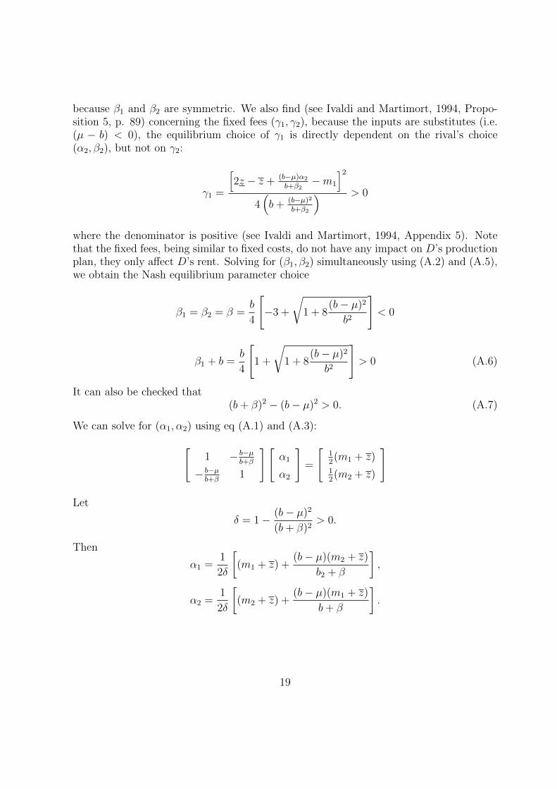
because β1 and β2 are symmetric. We also find (see Ivaldi and Martimort, 1994, Propo-sition 5, p. 89) concerning the fixed fees (γ1, γ2), because the inputs are substitutes (i.e.(µ − b) < 0), the equilibrium choice of γ1 is directly dependent on the rival’s choice(α2, β2), but not on γ2:

γ1 =

[2z − z + (b−µ)α2

b+β2−m1

]24(b+ (b−µ)2

b+β2

) > 0

where the denominator is positive (see Ivaldi and Martimort, 1994, Appendix 5). Notethat the fixed fees, being similar to fixed costs, do not have any impact on D’s productionplan, they only affect D’s rent. Solving for (β1, β2) simultaneously using (A.2) and (A.5),we obtain the Nash equilibrium parameter choice

β1 = β2 = β =b

4

[−3 +

√1 + 8

(b− µ)2

b2

]< 0

β1 + b =b

4

[1 +

√1 + 8

(b− µ)2

b2

]> 0 (A.6)

It can also be checked that(b+ β)2 − (b− µ)2 > 0. (A.7)

We can solve for (α1, α2) using eq (A.1) and (A.3):[1 − b−µ

b+β

− b−µb+β

1

][α1

α2

]=

[12(m1 + z)

12(m2 + z)

]

Let

δ = 1− (b− µ)2

(b+ β)2> 0.

Then

α1 =1

2δ

[(m1 + z) +

(b− µ)(m2 + z)

b2 + β

],

α2 =1

2δ

[(m2 + z) +

(b− µ)(m1 + z)

b+ β

].

19

References

[1] Antras, P. (2003), Firms, Contracts, and Trade Structure, Quarterly Journal of Eco-nomics, 118: 1375-1418.

[2] Antras, P. and E. Helpman (2004), Global Sourcing, Journal of Political Economy,122: 552-580.

[3] Antras, P. and E. Helpman (2008), Contractual Frictions and Global Sourcing. In:Helpman, E., Marin, D., and Verdier, T. (eds), The Organization of Firms in a GlobalEconomy. Harvard University Press: Cambridge, MA.

[4] Bernheim, D. and M. Whinston (1986a), Common Agency, Econometrica, 54: 923-942.

[5] Bernheim, D. and M. Whinston (1986b), Menu Auctions, Resource Allocations andEconomic Influence, Quarterly Journal of Economics, 101: 1-31.

[6] Bonnet, C., P. Dubois and S. Villas-Boas (2012), Empirical Evidence on the Roleof Non Linear Pricing and Vertical Restraints on Cost Pass-Through, Review ofEconomics and Statistics, forthcoming.

[7] Bulow, J., J. Geanakoplos and P. Klemperer (1985), Multimarket oligopoly: Strategicsubstitutes and complements, Journal of Political Economy, 93: 488-511.

[8] Draganska, M., D. Klapper and S. Villas-Boas (2010), A Larger Slice or a LargerPie: An Empirical Investigation of Bargaining Power in the Distribution Channel,Marketing Science, 29: 57-74.

[9] Eaton, J. and G.M. Grossman (1986), Optimal Trade and Industrial Policy underOligopoly, Quarterly Journal of Economics, 101: 383-406.

[10] Egger, P. and H. Egger (2005), Labour Market Effects of Outsourcing under Indus-trial Interdependence, International Review of Economics and Finance, 14: 349-363.

[11] Feenstra, R. (1998), Integration of Trade and Disintegration of Production in theGlobal Economy, Journal of Economic Perspectives, 12: 31-50.

[12] Feenstra, R. and G. Hanson (1996), Globalization, Outsourcing, and Wage Inequality,American Economic Review, 86: 240-245,

[13] Grossman, G.M. and E. Rossi-Hansberg (2008), Trading Tasks: A Simple Theory ofOffshoring, American Economic Review, 98: 1978-1997.

[14] Grossman, G., Helpman, E. (2003), Outsourcing versus FDI in Industry Equilibrium,Journal of the European Economic Association, 1: 317-327.

20

[15] Gu, W., G. Sawchuk and L. Rennison (2003), The effect of tariff reductions onfirm size and firm turnover in Canadian manufacturing, Review of World Economics(Weltwirtschaftliches Archiv), 139: 440-459.

[16] Head, K. and J. Ries (1999), Rationalization effects of tariff reductions, Journal ofInternational Economics, 47: 295-320.

[17] Helpman, E. (1984), A simple theory of trade with multinational corporations, Jour-nal of Political Economy, 92: 451-571.

[18] Helpman, E. and P. Krugman (1985), Market Structure and Foreign Trade, MITPress, Cambridge.

[19] Ivaldi, M. and D. Martimort (1994), Competition under Nonlinear Pricing, Annalesd’Economie et de Statistique, 34: 71-114.

[20] Long, N.V., H. Raff and F. Stahler (2011), Innovation and Trade with HeterogeneousFirms, Journal of International Economics, 84: 149-159.

[21] Martimort, D. (1992), Multi-Principaux avec Anti-Selection, Annales d’Economie etde Statistiques, 28: 1-38.

[22] Martimort, D. (2006), Multi-contracting mechanism design, in: Advances in eco-nomics and econometrics, Vol. 1., Cambridge University Press: 57-101.

[23] McCalman, P. (2012), Supersizing International Trade, University of Melbourne,mimeo.

[24] Melitz, M.J. (2003), The impact of trade on intra-industry reallocations and aggre-gate industry productivity, Econometrica, 71: 1695-1725.

[25] Miravete, E. (2002), Estimating Demand for Local Telephone Service with Asym-metric Information and Optional Calling Plans, Review of Economic Studies, 69:943-971.

[26] Stole, L. (1991), Mechanism Design under Common Agency, mimeo.

21