International Conference on Environmental Observations, International Conference on Environmental Observations, Modeling and Information Systems ENVIROMIS-2004Modeling and Information Systems ENVIROMIS-2004

17-25 July 2004, Tomsk, Russia17-25 July 2004, Tomsk, Russia

Mathematical modeling of natural and anthropogenic change of regional climate and environment

V.N. Lykosov

Russian Academy of Sciences Institute for Numerical Mathematics, Moscow E-mail: lykossov@inm.ras.ru

Climate SystemClimate System

• 1. ATMOSPHERE – the gas envelope of the Earth (oxygen, nitrogen, carbon dioxide, water vapor, ozone, etc.), which controls the solar radiation transport from space towards the Earth surface.

• 2. OCEAN – the major water reservoir in the system, containing salted waters of the World ocean and its seas and absorbing the basic part of the incoming solar radiation (a powerful accumulator of energy).

• 3. LAND – surface of continents with hydrological system (inland waters, wetlands and rivers), soil (e.g. with groundwater) and cryolithozone (permafrost).

• 4. CRYOSPHERE – continental and see ice, snow cover and mountain glaciers.

• 5. BIOTA – vegetation on the land and ocean, alive organisms in the air, water and soil, mankind.

The Climate SystemThe Climate System((TT. . Slingo, 2002)Slingo, 2002)

Annually mean air temperature in Khanty-Mansiisk for the time period from 1937 to 1999 (Khanty-Mansiisk

Hydrometeocenter).

-3

-2,5

-2

-1,5

-1

-0,5

0

Decades

C d

egre

es

Air temperature. May 2003 (Khanty-Mansiisk

Hydrometeocenter)

0

5

10

15

20

25

30

1 2 3 4 5 6 7 8 9 10 11 12 13 14 15 16 17 18 19 20 21 22 23 24 25 26 27 28 29 30 31

C d

egre

es

Среднесуточная температура Максимальная температура

Средняя температура Норма

Features of the climate system as physical object-IFeatures of the climate system as physical object-I

• Basic components of the climate system – atmosphere and ocean – are thin films with the ratio of vertical scale to horizontal scale about 0.01-0.001.

• On global and also regional spatial scales, the system can be considered as quasi-twodimensional one. However, its density vertical stratification is very important for correct description of energy cycle.

• Characteristic time scales of energetically important physical

processes cover the interval from 1 second (turbulence) to tens and hundreds years (climate and environment variability).

• Laboratory modelling of such system is very difficult.

Features of the climate system as physical object-IIFeatures of the climate system as physical object-II

• It is practically impossible to carry out specialized physical experiments with the climate system.

• For example, we have no possibility to “pump” the atmosphere by the

carbon dioxide and, keeping other conditions, to measure the system response.

• We have shirt–term series of observational data for some of

components of the climate system.

• Conclusion: the basic (but not single) tool to study the climate system dynamics is mathematical (numerical) modeling.

• Hydrodynamical climate models are based on global models of the atmosphere and ocean circulation.

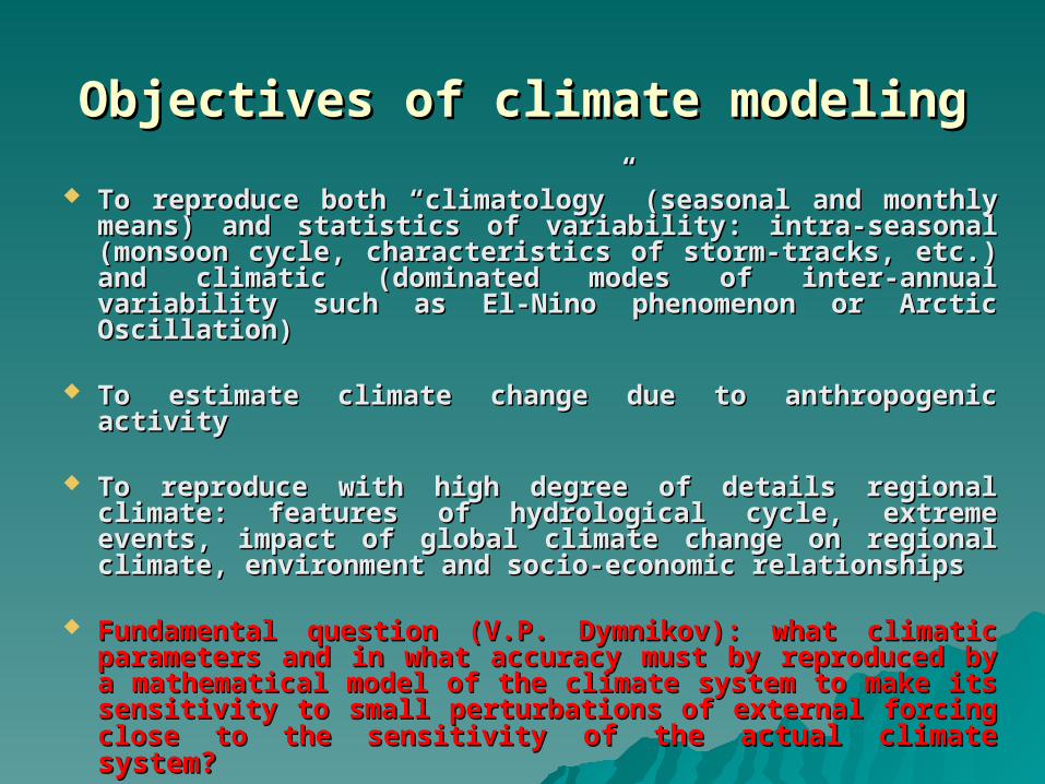
Objectives of climate modelingObjectives of climate modeling

To reproduce both “climatology” To reproduce both “climatology” ((seasonal and monthly means) and seasonal and monthly means) and statistics of variabilitystatistics of variability: : intra-seasonal intra-seasonal ((monsoon cycle, monsoon cycle, characteristics of storm-tracks, etc.characteristics of storm-tracks, etc.) ) and climatic and climatic ((dominated modes dominated modes of inter-annual variability such as El-Nino phenomenon or Arctic of inter-annual variability such as El-Nino phenomenon or Arctic Oscillation) Oscillation)

To estimate climate change due to anthropogenic activityTo estimate climate change due to anthropogenic activity

To reproduce with high degree of details regional climate: features of To reproduce with high degree of details regional climate: features of hydrological cycle, extreme events, impact of global climate change hydrological cycle, extreme events, impact of global climate change on regional climate, environment and socio-economic relationships on regional climate, environment and socio-economic relationships

Fundamental question (V.P. Dymnikov): what climatic parameters Fundamental question (V.P. Dymnikov): what climatic parameters and in what accuracy must by reproduced by a mathematical model and in what accuracy must by reproduced by a mathematical model of the climate system to make its sensitivity to small perturbations of of the climate system to make its sensitivity to small perturbations of external forcing close to the sensitivityexternal forcing close to the sensitivity of the actual climate of the actual climate system? system?

Computational technologiesComputational technologies

• Global climate model (e.g. model with improved spatial resolution in the region under consideration) implemented on computational system of parallel architecture (CSPA)

• Methods of “regionalization”: 1) statistical approach (“downscaling”);

2) hydrodynamical mesoscale simulation ( e.g., mesoscale model ММ5) requires CSPA;

3) large-eddy simulation of geophysical boundary layers (requires CSPA)

• Assessment of global climate change and technological impact on regional environment

Observational data to verify models

• 1) ECMWF reanalysis ERA-15 (1979-1993 г.г.), ERA-40 (1957-2001) http://www.ecmwf.int/research/era

• 2) NCEP/NCAR (National Center of Environment Protection/National Center of Atmospheric Research, USA), 1958-1997,

http://wesley.wwb.noaa.gov/reanalysis.htm

• 3) Precipitation from 1979 to present time http://www.cpc.ncep.noaa.gov/products/globalprecip

• 4) Archive NDP048, containing multiyear data of routine observations

on 225 meteorological stations of the former USSR http://cdiac.esd.oml.gov/ftp/ndp048

• Numerical experiments with modern global climate models produce a

large amount of data (up to 1Gb for 1 month). This requires special efforts for its visualization, postprocessing and analysis.

Large-scale hydrothermodynamics of the atmosphere uF

RT

av

a

uf

dt

du

cos

1tg ,

vFRT

au

a

uf

dt

dv

1

tg ,

RT

,

0cos

cos

1

vu

at,

Tp

Fa

v

a

u

tc

RT

dt

dT

cos ,

),( ECFdt

dqq

where

a

v

a

u

tdt

d

cos.

Subgrid-scaleprocesses

parameterization

Parameterization of subgrid-scale processesParameterization of subgrid-scale processes

• Turbulence in the atmospheric boundary layer, upper ocean layer and bottom boundary layer

• Convection and orographic waves

• Diabatic heat sources (radiative and phase changes, cloudiness, precipitation, etc.)

• Carbon dioxide cycle and photochemical transformations • Heat, moisture and solute transport in the vegetation and snow cover • Production and transport of the soil methane

• Etc.

T.J. Philips et al. (2002). Large-Scale Validation of AMIP II Land-Surface Simulations

Table 2. Model codes and features of the sixteen AMIP2 models analysed in Zhang et al. (2002)

Land-surface components No. of layers

in soil moist.

calculations

Model

Country

Code Resolution

Soil model

complexity

Canopy representation

No. of layers

in soil temp.

calculations

A

B

C

D

E

F

G

H

I

J

K

L

M

N

O

P

T42L18

T63L45

4x5 L21

T159L50

T63L30

T42L18

T62L18

T42L18

3.75x2.5 L58

3.75x2.5 L19

T47L32

4x5 L20

T42L30

T42L18

4x5 L24

4x5 L15

bucket

force-restore

multi-layer diffusion

multi-layer diffusion

multi-layer diffusion

multi-layer diffusion

multi-layer diffusion

multi-layer diffusion

multi-layer diffusion

multi-layer diffusion

multi-layer diffusion

multi-layer diffusion

multi-layer diffusion

multi-layer diffusion

bucket

bucket

const. canopy resistance

intercept. + transpiration

intercept. + transpiration

intercept. + transpiration

intercept. + transpiration

intercept.+transpiration+CO2

intercept. + transpiration

intercept. + transpiration

intercept.+transpiration+CO2

intercept.+transpiration+CO2

intercept. + transpiration

intercept. + transpiration

intercept. + transpiration

intercept.+transpiration+CO2

no

no

3

2

24

4

4

6

3

2

4

4

3

2

3

6

1

1

1

2

24

4

3

6

2

3

4

4

3

3

3

6

1

1

CCSR, Japan

CNRM, France

INM, Russia

ECMWF, UK

JMA, Japan

NCAR, USA

NCEP, USA

PNNL, USA

UGAMP, UK

UKMO, UK

CCCMA, Can

GLA, USA

MRI, Japan

SUNYA, USA

UIUC, USA

YONU, Korea

The Taylor diagram for the variability of the latent heat flux at the land surface as follows from results of AMIP-II experiments

(Irannejad et al., 2002).

Sensitivity of the climate Sensitivity of the climate system to small perturbations system to small perturbations

of of external forcingexternal forcing

(invited lecture at the World Climate (invited lecture at the World Climate Conference, Moscow, 29 September – 3 October, Conference, Moscow, 29 September – 3 October,

2003)2003)

V.P. Dymnikov, E.M. Volodin, V.Ya. Galin, A.S. Gritsoun, A.V. Glazunov, N.A. Diansky, V.N. Lykosov

Institute of Numerical Mathematics RAS, Moscow

AGCM - Finite difference model with spatial resolution 5°x4° and 21 levels in sigma-coordinates from the surface up to 10 hPa. - In radiation absorption of water vapour, clouds, CO2, O3, CH4, N2O, O2 and aerosol are taken into account. Solar spectrum is divided by 18 intervals, while infrared spectrum is divided by 10 intervals. - Deep convection, orographic and non-orographic gravity wave drag are considered in the model. Soil and vegetation processes are taken into account.

||

Non-flux-adjusted coupling

||

OGCM -The model is based on the primitive equations of the ocean dynamics in spherical sigma-coordinate system. It uses the splitting-up method in physical processes and spatial coordinates. Model horizontal resolution is 2.5°x2°, it has 33 unequal levels in the vertical with an exponential distribution.

INM coupled atmosphere - ocean general

circulation model

The climate model sensitivity to the increasing of CO2

CMIP - Coupled Model Intercomparison Project

http://www-pcmdi.llnl.gov/cmip

CMIP collects output from global coupled ocean-atmosphere general circulation models (about 30 coupled GCMs). Among other usage, such models are employed both to detect anthropogenic effects in the climate record of the past century and to project future climatic changes due to human production of greenhouse gases and aerosols.

Response to the increasing of CO2CMIP models (averaged)

INM model

Global warming in CMIP models in CO2 run and parameterization of lower inversion clouds

T - global warming (K), LC - parameterization of lower inversion clouds (+ parameterization was included, - no parameterization, ? - model description is not available). Models are ordered by reduction of global warming.

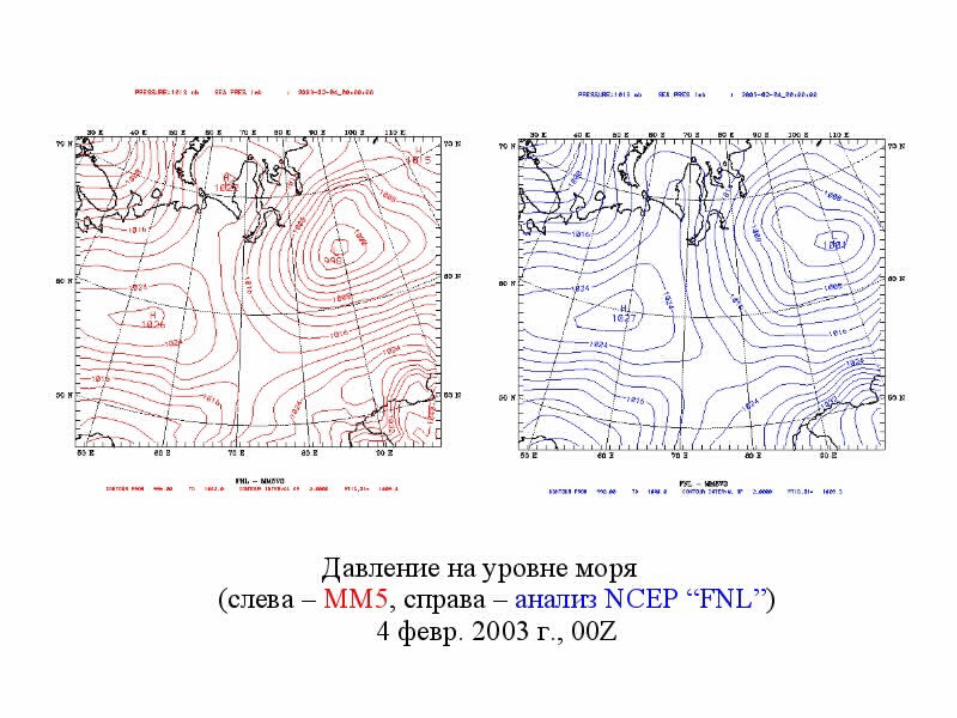
Mesoscale non-hydrostatic modelingMesoscale non-hydrostatic modeling

• MM5 - Penn State/NCAR Mesoscale Modeling System http://www.mmm.ucar.edu/mm5

• Program code: Fortran77, Fortran90, C. Hybrid parallelization (shared and distributed memory) + vectorization

• Documentation• Implemented by V. Gloukhov

(SRCC/MSU) on MVS-1000M

International Conference on International Conference on Computational Mathematics ICCM-2004, Computational Mathematics ICCM-2004,

21-25 June, 2004, Novosibirsk, Russia21-25 June, 2004, Novosibirsk, Russia

Large-Eddy Simulation of Geophysical Boundary Layers on Parallel Computational Systems V.N. Lykosov, A.V. Glazunov Russian Academy of Sciences Institute for Numerical Mathematics, Moscow E-mail: lykossov@inm.ras.ru, glazunov@inm.ras.ru

Geophysical Boundary Layers (GBLs) as Geophysical Boundary Layers (GBLs) as elements of the Earth climate systemelements of the Earth climate system

• Atmospheric Boundary Layer HABL ~ 102 - 103 m• Oceanic Upper Layer HUOL ~ 101 - 102 m• Oceanic Bottom Layer HOBL ~ 100 - 101 m

GBL processes control:

• 1) transformation of the solar radiation energy at the atmosphere-Earth interface into energy of atmospheric and oceanic motions

• 2) dissipation of the whole Earth climate system kinetic energy

• 3) heat- and moisture transport between atmosphere and soil (e.g. permafrost), sea and underlying ground (e.g. frozen one).

Dynamic structure of GBLsDynamic structure of GBLs

Three types of motion:

• totally organized mean flow• coherent semi-organized structures (large

eddies and waves)• chaotic three-dimensional turbulence

Turbulence in PBLsTurbulence in PBLs

● Rough surface● Large scales● Stratification

Inertial range

Dissipation range

Energy range

Synoptical variations

Boundary-Layer flows

Differential formulation of models Models are based on Reynolds’ type equations obtained after spatial averaging of Navier-Stokes equa-tions and added by equations of heat and moisture (or salt):

Turbulent ClosureTurbulent Closure

Equation for turbulent kinetic energy (of subgrid-scale motions):

Equation for turbulent kinetic energy dissipation:

Constraint on maximal value of sub-grid turbulence length scale:

3/ 2

,c E

l

• Finite-difference approximation on “C” grid

• Explicit time scheme of predictor-corrector type (Matsuno scheme)

Numerical schemeNumerical scheme

Calculation of tendencies

diffusionCoriolis forcegravityadvection

pressure gradient

diffusionadvection

diffusionadvection

Boundary conditions

Velocity componentsCalculation of

eddy viscosity and diffusioncoefficients

Summing up of tendencies

ТКЕ, ТКЕ dissipation

Temperature, moisture, salinity Solver for the Poisson equation

Calculation of the Poisson equation R.H.S.

Input-output,post-processing

ТКЕ,ТКЕ

dissipation

production, dissipation, non-linear terms

velocity componentstemperature,

moisture, salinity ТКЕ, ТКЕ dissipation

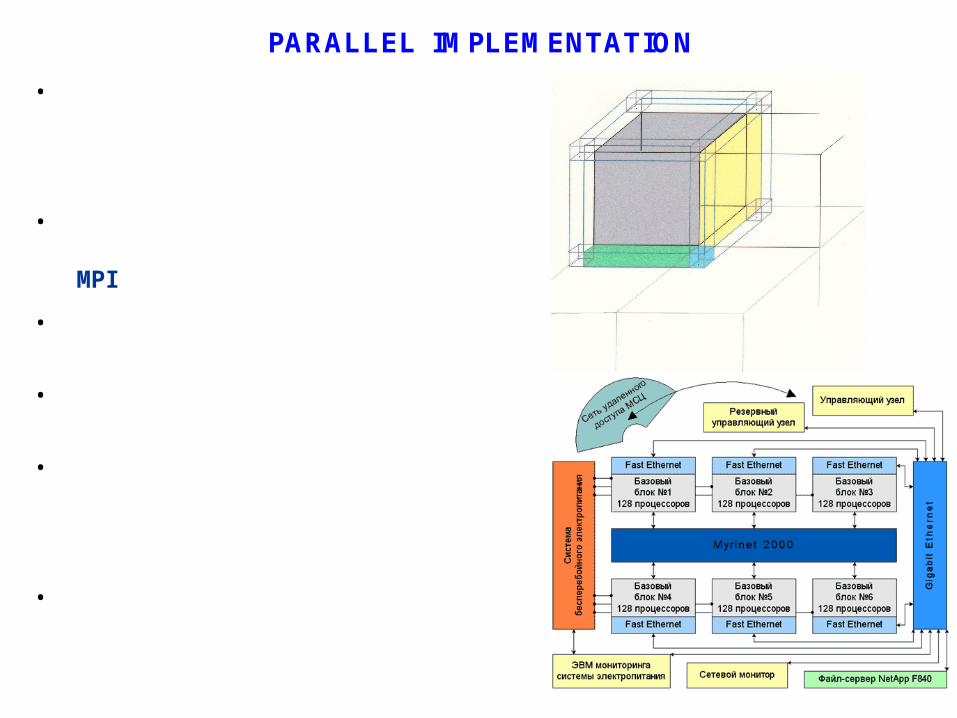
PARALLEL IMPLEMENTATION

• Parallel version of models is developed to be mainly used on supercomputers with distributed memory

•Procesor-to-processor data exchange is realized with the use of MPI standard

• non-blocked functions of the data transfer-receive

•3-D decomposition of computational domain

• on each time step, processes are co-exchanged only by data which belongs to boundary grid cells of decomposition domains

• The Random Access Memory (operative memory) is dynamically distributed between processors (the features of FORTRAN-90 are used)

• Debuging and testing of parallel versions of models is executed on supercomputer MVS1000-М of Joint Supercomputer Center (768 processors, peak productivity - 1Tflops)

3% 6%

7%

2%

10%

1%

13%

58%

exchanges

diffusion

advection of scalars

advection of momentum

turbulent closure

boundary condition

additional procedures

Poisson equationincludig exchanges

“Extreme” case: Domain 768 x 768 x 256 (= 150 994 994) grid points 574 processors 3D decomposition (12 x 12x 4) MGD Poisson solver 15 Gbytes of memory 1 step of scheme ~ 20 s of computer time.

Spectra of kinetic energy calculated using results of large-eddy simulation of the convective upper oceanic layer under different spatial resolution (m3)

von Karman votrex street behind a round cylinder, Re =200: top - from М. ван Дайк (1986). Альбом течений жидкости и газа, bottom - model results

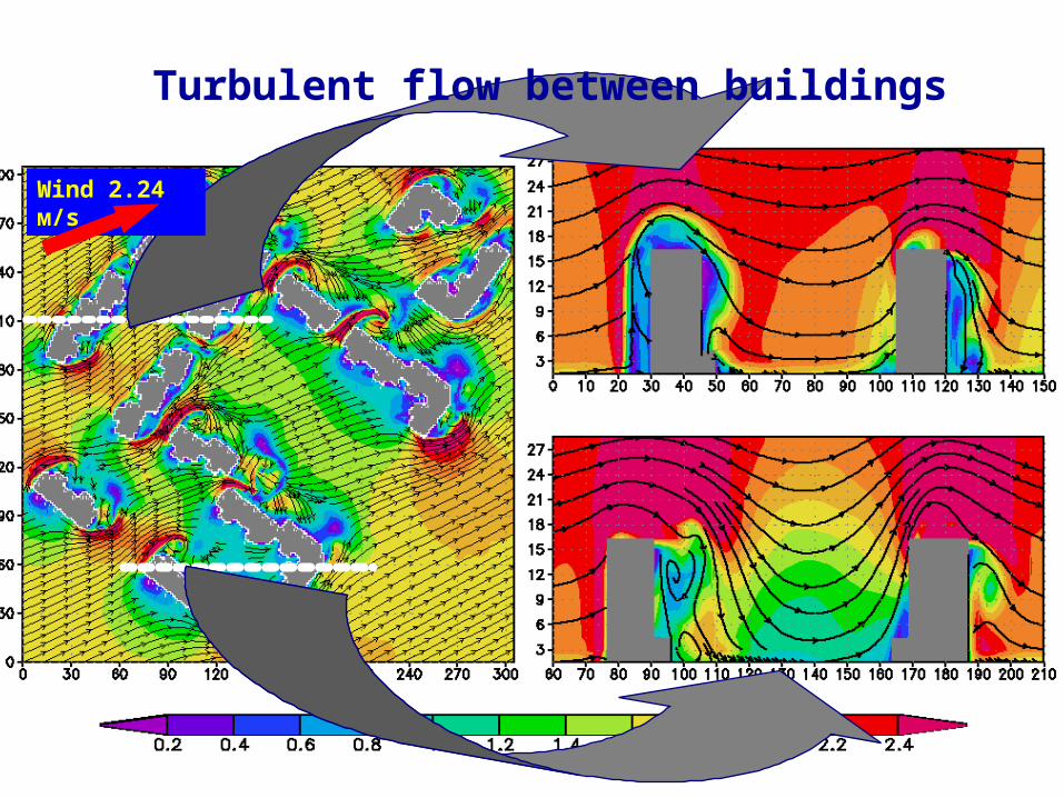
Turbulent flow between buildings

Wind 2.24 м/s

Lagrangian transport of fine-dispersive particle tracer Large number of particles in turbulent flow generated by the LES-model of the atmospheric boundary layer.

The calculation of trajectories is carried out simultaneously with numerical integration of the hydrodynamic part of the model.

● It is assumed that each of particles has non -zero mass and size. It is possible to sort particles in few groups accordingly to their size and density.

The code of tracer transport is parallelized with the use of MPI. The data exchange between processors is

realized with the help of non-blocking transfers and takes place on the background of basic calculations. Using results of calculations, the spatial distribution of the particle tracer concentration is calculated for each

time step. On parallel computational system this algorithm allows to simultaneously calculate trajectories of tens

millions particles. The time which is needed to calculate the particles transport is significantly less then the time of the ABL model integration.

● Equation of the particle motion in the air flow: where xi (i=1,2,3) – particle coordinates, m – mass of particle, f – drag force. ● To calculate f , the Stokes formula is used:

,3mgfxm iii

6 ( )ii if r V x

An example of the particle transport by the turbulent flow between buildings

Wind Particle concentration

Particles are ejecting near the surface (along the dotted line). The maximal number of particles is about 10 000 000.

Snow

“Upper” ice

Water

Ground

“Lower” ice

U

H,LE Es

EaS

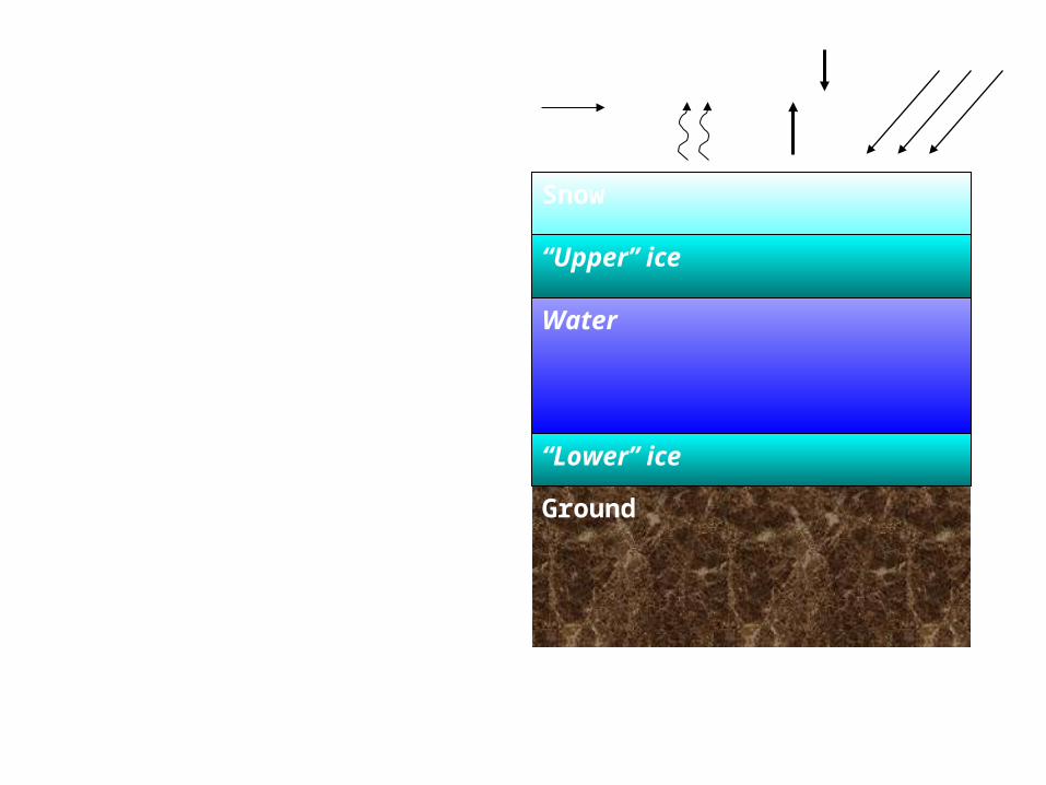
Thermodynamics of shallow Reservoir (Stepanenko & Lykosov, 2003, 2004)

1) One-dimensional approximation.

2) On the upper boundary: fluxes of momentum, sensible and latent heat, solar and long-wave radiation are calculated On the lower boundary: fluxes are prescribed

3) Water and ice: heat transport Snow and ground: heat- and moisture transport

U – wind velocityH – sensible heat fluxLE – latent heat fluxS – shirt-wave radiationEa – incoming long-wave radiation Es – outgoing long-wave radiation

Mathematical formulation

- for water and ice:

, - heat conductivity

- for snow:

- temperature

- liquid water

- for ground:

- temperature

- liquid water

- ice

2

2 2

1 dhT T dh T T Iñ c c

t h dt h h dt z

h

z

.

,

fr

fr

Fzt

W

LFz

T

zt

Tс

.

,

,

i

iW

iiWT

Ft

I

Fzz

W

zt

W

FLz

WTc

z

T

zt

Tc

Kolpashevo

0 5 10 15 20 25 30

-40

-35

-30

-25

-20

-15

-10

-5

Температура поверхности снега, Колпашево, 02.1961

Данные натурных экспериментов Результаты моделирования

Тем

пер

ату

ра, С

Время, дни

Simulated snow surface temperature versus measured one on meteorologicalstation Kolpashevo (1961)

0 5 10 15 20 25 30 35

-50

-40

-30

-20

-10

0

Температура поверхности снега, 01.61

EДанные натурных измерений EРезультаты моделирования

Тем

пер

атур

а,

С

Время, дни

Quality of snow surface temperature reproduction is an indicator of quality of heat transfer parameterization in the “atmospheric surface layer – snow” system.

Accuracy of temperature measurementson meteorological station is about 0.5 ℃.

Syrdakh Lake

-4 -3 -2 -1 0 1 2 3 4 5

5

4

3

2

1

0

наблюдения эмпир. параметр. e-параметр.

Гл

уби

на,

мТемпература, С

Рис. 11.Вертикальный профиль температуры в оз. Сырдах, апрель 1977 г.

3 4 5 6 7 8 9 10 11 12 13 14 15 16 17 18 19

5

4

3

2

1

0

наблюдения эмпир. параметр. e-параметр.

Гл

уби

на

, мТемпература, С

Рис. 13.Вертикальный профиль температуры в оз. Сырдах, июнь 1977 г.

Ground temperature under Syrdakh Lake (modeling results)

As follows from results of numerical experiments, the talik is stably existing during all of integration time (20 years, 1965-1984). Its depth varies from 1.2 to 2 meters under the lake bottom.

THANK YOUTHANK YOU

for YOUR ATTENTIONfor YOUR ATTENTION