international financial spillovers to emerging market economies
TRANSCRIPT

K.7
International Financial Spillovers to Emerging Market Economies: How Important Are Economic Fundamentals? Ahmed Shaghil, Brahima Coulibaly, and Andrei Zlate
International Finance Discussion Papers Board of Governors of the Federal Reserve System
Number 1135 April 2015
Please cite paper as: Ahmed Shaghil, Brahima Coulibaly, and Andrei Zlate (2015). International Financial Spillovers to Emerging Market Economies: How Important Are Economic Fundamentals? International Finance Discussion Papers 1135. http://dx.doi.org/10.17016/IFDP.2015.1135

Board of Governors of the Federal Reserve System
International Finance Discussion Papers
Number 1135
April 2015
International Financial Spillovers to Emerging Market Economies: How Important Are Economic Fundamentals?
Shaghil Ahmed, Brahima Coulibaly, Andrei Zlate* NOTE: International Finance Discussion Papers are preliminary materials circulated to stimulate discussion and critical comment. References to International Finance Discussion Papers (other than an acknowledgment that the writer has had access to unpublished material) should be cleared with the author or authors. Recent IFDPs are available on the Web at www.federalreserve.gov/pubs/ifdp/. This paper can be downloaded without charge from the Social Science Research Network electronic library at www.ssrn.com.

International Financial Spillovers to Emerging Market Economies: How Important Are Economic Fundamentals?
Shaghil Ahmed, Brahima Coulibaly, Andrei Zlate*
April 2015
Abstract We assess the importance of economic fundamentals in the transmission of international shocks to financial markets in various emerging market economies (EMEs). Our analysis covers the so-called taper-tantrum episode of 2013 and six earlier episodes of severe EME-wide financial stress since the mid-1990s. Cross-country regressions lead us to the following results: (1) EMEs with relatively better economic fundamentals suffered less deterioration in financial markets during the 2013 taper-tantrum episode. (2) Differentiation among EMEs set in quite early and persisted throughout this episode. (3) Controlling for economic fundamentals, we also find that, during the taper tantrum, financial conditions deteriorated more in those EMEs that had earlier experienced larger private capital inflows and greater exchange rate appreciation. (4) For earlier episodes, we find little evidence of investor differentiation across EMEs being explained by differences in their relative vulnerabilities during EME crises of the 1990s and early 2000s. (5) That said, differentiation across EMEs based on fundamentals does not appear to be unique to the 2013 episode. Differences in economic fundamentals played a role in explaining the heterogeneous EME financial market responses during the global financial crisis of 2008, and the role of fundamentals appeared to progressively increase through the European crisis in 2011 and subsequently the 2013 taper tantrum. Keywords: Emerging market economies, financial spillovers, economic fundamentals, vulnerability, depreciation pressure, taper tantrum, financial stress. JEL classifications: E5, F3.
*Shaghil Ahmed ([email protected]) and Brahima Coulibaly ([email protected]) are economists in the Division of International Finance, Board of Governors of the Federal Reserve System, Washington, D.C. 20551 U.S.A. Andrei Zlate ([email protected]) is a financial economist in the Department of Supervision, Regulation, and Credit at the Federal Reserve Bank of Boston, 600 Atlantic Avenue, Boston, MA 02210, U.S.A. We thank Steve Kamin, Prachi Mishra, Patrice Robitaille, as well as participants at the American Economic Association 2015 annual meetings and the Federal Reserve Board conference on “Spillovers from Accommodative Monetary Policies since the GFC” for very useful comments. We also thank Zina Saijid and Julio Ortiz for outstanding research assistantship. The views expressed in the paper are those of the authors and should not be interpreted as reflecting the views of the Board of Governors of the Federal Reserve System or any other person associated with the Federal Reserve System.

1 Introduction
Starting in May 2013, on news that the Federal Reserve could soon start tapering its large scale
asset purchases (LSAPs), financial conditions in emerging market economies (EMEs) deteriorated
sharply. Investors withdrew capital, currencies depreciated, stock markets fell, and bond yields
and premiums on credit default swaps rose. This so-called taper-tantrum episode sparked debate
on how foreign economies may be affected– and which economies, especially among the EMEs,
may experience the most adverse effects– once the process of U.S. monetary policy normalization
begins.
Indeed, one intriguing feature of the “risk-off” episode during the summer and fall of 2013
was that it did not have a similar effect on all EMEs. While some countries experienced acute
deteriorations in financial conditions, others were much less affected. The varied experiences of the
different EMEs have spawned research on whether the heterogeneous response of EME financial
markets during the taper tantrum can be explained by differences in economic fundamentals across
these economies. (See, for example: Prachi et al., 2014; Eichengreen and Gupta, 2014; Aizenman et
al., 2014; and Sahay et al., 2014.) And, these experiences have also focused attention on whether,
more broadly, the effects of U.S. monetary policy shocks on EMEs over a longer period have been
related to these economies’own vulnerabilities (Bowman et al., 2014).
In this paper, we seek to contribute to this sparse but growing literature. Specifically, we address
three questions: First, to what extent did investors differentiate among the EMEs based on their
economic fundamentals during the “risk-off”episode of 2013? Or, can the heterogeneous responses
across EMEs be explained by other factors, such as whether those economies that initially received
the heaviest capital inflows were also the ones from which investors receded the most during the
episode, a possibility raised by some researchers such as Aizenman et al. (2014). Second, during
the taper-tantrum stress episode, when exactly did differentiation across EMEs begin and how
persistent was it? Did investors initially display herd behavior and pull back indiscriminately
from all EMEs, and then only begin differentiating over time as the shock persisted? Or did they
discriminate across EMEs from the early stages of the episode? Third, is the differentiation across
EMEs by investors a relatively recent phenomenon, or does the application of our methodology
suggest that investors have always distinguished among EMEs to some extent according to their
economic fundamentals?
1

Research to date has not appeared to reach a consensus on the first question– the importance
of fundamentals in explaining the heterogeneous EME responses. Using an event study approach,
Prachi et al. (2014) analyze the reaction of financial markets to the Federal Reserve’s LSAPs
tapering announcements in 2013 and 2014, including the episode that we examine in this study.
They find evidence of market differentiation among EMEs based on macroeconomic fundamentals.
In addition, they find that EMEs with deeper financial markets and tighter macroprudential policy
prior to the stress period experienced relatively less deterioration in financial conditions.
In contrast, Eichengreen and Gupta (2014) do not find evidence that better macroeconomic
fundamentals– such as a lower budget deficit, lower public debt, a higher level of international re-
serves, and higher economic growth– provided any insulation. They do find, however, that EMEs
whose exchange rates appreciated more earlier and whose current account deficits widened more
experienced a larger effect. But they conclude that the heterogeneous reactions most importantly
owed to the size of each country’s financial market; larger markets experienced more pressure, as in-
vestors were better able to rebalance their portfolios in these EMEs with relatively large and liquid
financial markets. Similarly, Aizenman et al. (2014) find no evidence that stronger macroeconomic
fundamentals helped the EMEs weather the taper tantrum better, but their study focuses only on
the very short-term responses of financial indicators after taper news. Classifying EMEs into two
categories (“fragile”and “robust”) based on their current account balances, levels of international
reserves, and external debt, they find that news of tapering from Fed Chairman Bernanke was
associated with sharper deterioration of financial conditions in the “robust”EMEs compared with
the “fragile”ones in the very short term (24 hours following the announcement). The authors ra-
tionalize their results by conjecturing that EMEs with stronger fundamentals received more capital
inflows during the expansionary phase of the Federal Reserve’s conventional and unconventional
monetary policy and accordingly experienced sharper capital outflows and deteriorations in finan-
cial conditions on news of an impending tapering. This hypothesis is not explicitly tested in their
study, and the authors acknowledge that, over a longer window than they considered in their event
study, the fragile EMEs may have suffered more than robust EMEs after the taper news.
We approach the first question in a somewhat different manner from these previous studies.
Rather than looking at market reactions on days when news may be coming in about the Federal
Reserve’s tapering of asset purchases as Prachi et al. (2014) do, we treat the taper tantrum as a
single episode, defined by the observed “peak-to-trough”behavior of financial markets surrounding
2
the period when concerns about tapering came to the forefront. And unlike Aizenman et al. (2014),
but consistent with Prachi et al. (2014), we exploit finer cross-section differences in vulnerabilities
across the EMEs rather than divide the EMEs into two groups based on the behavior of only three
variables. Using a sample of 20 emerging market economies and cross-section regression analysis,
we assess the role of economic fundamentals in the heterogeneous cumulative performance of EME
financial markets over the whole episode from May 2013 through August 2013.
We find that EMEs that had relatively better fundamentals to begin with– as measured by
a host of individual variables capturing vulnerability as well as an aggregate index of relative
vulnerabilities across EMEs that we construct– suffered less deterioration during the taper-tantrum
episode as measured by a broad range of financial variables, including exchange rate, depreciation
pressure, and government bond yields, as well as EMBI and CDS spreads. Our results are consistent
with those in Prachi et al. (2014), but contrast with those in Aizenman et al. (2014) and Eichengreen
and Gupta (2014). We also find that financial conditions deteriorated more in those EMEs that had
earlier experienced larger private capital inflows and exchange rate appreciations, consistent with
the “more-in-more-out”hypothesis that EMEs that experienced larger inflows prior to the taper
tantrum also experienced larger outflows once the episode began. Also, we find some evidence
that the structure of the financial markets– such as the size of the capital market, the level of
foreign investor participation, the extent of capital account openness, or revisions to the growth
outlook– shaped the heterogeneous responses of some financial indicators, as in Eichengreen and
Gupta (2014). However, the strength of economic fundamentals explains much more of the variation
in responses across EMEs compared with other factors, such as the previous runup in flows or the
structure of financial markets.
On the second question, related to the timing and persistence of differentiation, the conventional
wisdom seems to be that early in the taper tantrum, investors did not differentiate much among
EMEs according to their vulnerabilities, but such differences emerged when concerns about tapering
persisted. (See, for example, Sahay et al., 2014). However, our evidence suggests that differentiation
according to relative vulnerabilities set in relatively early during the stress episode and persisted
for some time, although the extent of differentiation was less pronounced in the first few weeks.
Turning to the third question of the extent to which investors also discriminated among EMEs
in the past, we use our methodology to identify six previous episodes of severe financial stress in the
EMEs over the past 20 years: the European sovereign debt crisis (2011), the global financial crisis
3

(GFC, 2008-09), the Argentine crisis (2002), the Russian crisis (1998), the Asian crisis (1997-98),
and the Mexican crisis (1994-95). For each of these episodes, we examine the role of economic
fundamentals in driving any heterogeneous cumulative reaction of asset prices over the full episode
across EMEs. We find little evidence of differentiation based on economic fundamentals in the
1990s and the early 2000s, consistent with literature on herding behavior of investors toward EMEs
and contagion during that period, such as Dornbusch et al. (2000) and Calvo and Mendoza (2001).
However, the results also suggest that differentiation was not unique to the taper tantrum in 2013.
In fact, it appears that fundamentals played a role in explaining the heterogeneous reaction of
EME asset prices during the GFC in 2008, and that their role increased during the European
sovereign crisis in 2011, and then increased further during the taper tantrum in mid-2013. These
results that differentiation has occurred among EMEs since the GFC are consistent with those
from a complementary approach taken in Bowman et al. (2014): identifying monetary policy-
related shocks to U.S. interest rates, rather than episodes of severe financial stress as we do, they
find that the effect of such shocks on EME interest rates have been larger in the relatively more
vulnerable EMEs in the recent past as well, and that there is no difference in this respect between
the effects of conventional and unconventional U.S. monetary policy.
Taken at face value, our results suggest that international investors may have moved from herd
behavior in the past– such as during the 1990s and the early 2000s– to progressively differentiating
more and more among EMEs according to their economic fundamentals through the GFC, the
European debt crisis, and the taper tantrum. It remains an open question, however, whether
our results are perhaps driven by different sources of the shock. The stress episodes since the
GFC, during which we find evidence of differentiation among EMEs, emanated primarily from the
advanced economies, whereas the crises of the 1990s and 2000s, during which we find little evidence
of differentiation, emanated to a much larger extent– although not exclusively so– from shocks
originating in the EMEs themselves.
The remainder of the study is organized as follows: In section 2, we describe the data and
the estimation strategy. Then, section 3 presents our results of differentiation across EMEs during
the 2013 taper-tantrum episode, and section 4 shows the results for differentiation in previous
well-recognized EME financial stress episodes. section 5 concludes.
4
2 Econometric specification and choice of variables
For each EME stress episode identified, we regress performance in selected financial markets across
EMEs over the duration of the stress period on a set of variables capturing economic conditions that
existed prior to the beginning of the stress episode and other control variables. Our cross-section
regression is represented by the following equation:
∆FinV ari,k = c+∑j
βi,jXi,j + εi (1)
Note that each i denotes a particular country, and each k denotes a particular financial variable
with its performance over the stress episode represented by ∆. Xi,j are a set of explanatory
variables j specific to country i measured in the year prior to the onset of the stress period, β’s are
parameters to be estimated, and ε’s are error terms. Data availability across countries and time
limits our sample to 20 EMEs.1 Note that the cross-section observations in each regression are
the countries, and a separate regression is run for each dependent variable k and each sub-set of
explanatory variables j.
Among the dependent variables measuring financial performance, we consider the percent
change in the country’s bilateral nominal exchange rate against the dollar, the change in the local
currency bond yields on 10-year government bonds, the percent change in the stock market in-
dex, and the change in EMBI and CDS spreads between the peak and trough of each episode (for
example, from April to August for the 2013 episode) using monthly data.2 Pressures on financial
markets may not necessarily be reflected in the exchange rate if the central bank intervenes in
foreign exchange markets to prop up the currency or raises the policy rate to contain capital flight.
For this reason, we also consider a depreciation pressure index that is a weighted average of the
change in the exchange rate and the foreign exchange reserves, following Eichengreen et al. (1995),
with the weights given by the inverse of the standard deviation of each financial indicator measured
in the cross section.3
1 Argentina, Brazil, China, Chile, Colombia, Indonesia, India, South Korea, Malaysia, Mexico, Peru, Paraguay,the Philippines, Pakistan, Russia, South Africa, Taiwan, Thailand, Turkey, and Uruguay. Although data for somecountries were available, we exclude euro-area countries, dollarized economies, and the EMEs with hard peg exchangerate regimes.
2 The monthly data reflect end-of-month values for exchange rates, foreign exchange reserves, and policy interestrates, and average monthly values for bond yields, stock market indices, and EMBI and CDS spreads.
3 Alternatively, we also constructed a depreciation pressure index based on the changes in exchange rates, foreignexchange reserves, and the policy rates between April and August 2013. Since the two indexes behave similarlyduring the taper-tantrum episode, our results are mostly based on the standard depreciation index based on changes
5

We consider several different types of independent variables: those that might be capturing
the macroeconomic fundamentals and policy choices of a country (category 1), those that might
help identify how much capital might have been flowing in prior to the episode so we can test
the “more-in-more out”hypothesis (category 2), and those that might be capturing aspects of a
country’s financial structure such as openness and financial development (category 3), which are
included as other control variables.
Potential candidates for category 1 include the following six variables reflecting the strength
of macroeconomic fundamentals: the current account balance as a percent of GDP; foreign exchange
reserves as a percent of GDP; short-term external debt as a percent of foreign exchange reserves;
the gross government debt as a percent of GDP; the average annual inflation over the past three
years; and the runup in bank credit to the private sector, measured as the change in the ratio
of bank credit to GDP over the five years prior. To mitigate concerns over endogeneity, each of
these is taken as of the year prior to the one in which the episode occurs. For the 2013 event,
we also use the revisions to the outlook for economic activity as an additional variable capturing
fundamentals since analysts were, at least anecdotally, pointing to this as an important factor.
The revisions to the outlook are measured as the change between January and May of 2013 in the
outlook for annual average real GDP growth for 2013 provided by Consensus Economics. Finally,
we account for the monetary policy and exchange rate frameworks through two indicator variables
with the first variable equal to 1 for countries operating under an inflation targeting regime and 0
if not, and the second variable equal to 1 for countries with floating exchange rate regimes based
on the classification in the IMF’s Annual Report on Exchange Rate Arrangements and Exchange
Restrictions, and 0 otherwise. Given the relatively small cross-section, not all of these variables can
be included simultaneously; we consider individual variables one at a time and sub-sets of them.
We also compute an aggregate index of relative vulnerabilities across the cross-section using some
of these variables in light of the limited number of observations; this vulnerability index is described
in detail in section 3.2.2.
For category 2, we include the following variables: the cumulative gross capital inflows over
the past three years as a percent of GDP and the appreciation of the real effective exchange over
the past three years. For category 3 variables, we consider the capitalization of the domestic equity
market as a share of GDP; foreign participation in the domestic equity market, measured as the
in exchange rates and reserves only.
6

share of foreign equity holdings in the domestic equity market; and capital account openness, as
measured by the Chinn-Ito index, a de jure measure of financial openness initially introduced in
Chinn and Ito (2008) and subsequently updated by the authors through 2011. For each of these
indicators, the data sources are presented in table 1.
3 Differentiation across EMEs during the 2013 taper-tantrum episode
This section provides an overview of the taper-tantrum episode of 2013, presents new evidence on
the drivers of EME differentiation for the entire duration of the episode, and discusses the timing
and persistence of differentiation within sub-intervals of the episode itself.
3.1 Overview of the episode
Market participants shifted their expectation for the Federal Reserve’s asset purchases program
following former Chairman Bernanke’s testimony to the Congress on May 22. The testimony
heightened perceptions that the Federal Reserve would soon begin tapering its LSAPs and thus
lessen the amount of monetary stimulus it was putting into the economy through its unconventional
monetary policies. This shift in market expectations led to sharp movements in U.S. and global
financial markets, including a large sell-off of EME assets by international investors, causing large
depreciations of currencies, increases in bond yields, EMBI spreads, and CDS spreads, as well as
declines in equity markets. As shown in table 1, for the median EME in our sample, the dollar
exchange rate depreciated 9 percent, sovereign bond yields rose almost 2 percentage points, the
EMBI and CDS spreads each rose 0.5 percentage point, and the stock market fell 5 percent from
April to August. In response, central banks in some EMEs intervened in the foreign exchange
markets to curb depreciation pressures, which resulted in losses of foreign exchange reserves, and
also, in some cases, raised policy rates to discourage capital flight. The stress episode persisted for
much of the summer, until the Federal Reserve chose not to reduce the size of its asset purchases at
the September 2013 Federal Open Market Committee meeting. Thus, we date the taper tantrum
episode from May to August and compute the change in financial indicators relative to April,
consistent with the literature.
Although most financial markets in EMEs were negatively affected during the taper tantrum,
there was wide dispersion in the financial performance across EMEs, as shown by the histograms
7

in figure 1. As can be seen in panel 1, although most EME currencies depreciated between 5 and
10 percent, the extent of depreciation did vary quite a bit, with some hardly depreciating at all,
while others depreciated more than 15 percent. The use of foreign exchange rate intervention and
the response of policy rates also appeared to vary across EMEs (panels 2 and 3, respectively).
The heterogeneous response is also apparent in the exchange rate pressure index that combines
changes in the exchange rate and foreign exchange reserves (panel 4). Similarly, the increases in
bond yields, EMBI spreads, and CDS spreads varied quite a bit across EMEs, as did the declines
in equity markets (panels 6-9).
With U.S. interest rates expected to rise, some effect on the EMEs was to be expected for
several reasons. For example, rising U.S. rates encourage investors to shift their holdings toward
U.S. assets. At the same time, investors may withdraw funds during risk-off episodes especially from
those EMEs perceived to be more risky. Indeed, although the movements in most EME financial
markets were sizable, investors did not appear to withdraw funds indiscriminately from all EMEs
en masse, as shown in figure 1. Therefore, we next turn to the question of whether the varied
response of EME financial markets during the taper tantrum episode was systematically related to
their economic fundamentals.
3.2 Differentiation across EMEs during the 2013 stress episode as a whole
As a first cut to examining this issue, we present some scatter plots capturing bivariate relationships.
Figure 2 plots exchange rate depreciations across EMEs during the episode (on the vertical axis)
against six potential variables (on the horizontal axis in the different panels) that investors may
care about when assessing a country’s macroeconomic fundamentals. The figure suggests that the
EMEs whose currencies depreciated by more also had larger current account deficits as a share of
GDP (panel 1), less reserves-to-GDP (panel 2), more short-term external debt as a share of reserves
(panel 3), higher gross government debt ratios (panel 4), and higher average inflation over the past
few years (panel 5). The only variable among the ones we show that did not seem to affect financial
market performance across EMEs is the runup in bank credit to the private sector as a ratio to
GDP (panel 6).
Figure 3 does a similar exercise of linking individual macroeconomic variables to the performance
of bond markets, specifically the rise in local currency bond yields during the taper tantrum. The
results obtained are generally consistent with those found in figure 2. Bond yield increases were
8

greater in economies with greater current account deficits, less reserves, higher short-term debt,
and higher average inflation. However, the gross government debt position and, again, the runup
in credit to the private sector were not correlated with changes in bond yields.
To further understand the drivers of the heterogeneous performance of EME financial markets,
we estimate equation (1) using explanatory variables from the three categories described in section
2, that is, first, those describing the strength of macroeconomic fundamentals, the growth outlook,
and the policy framework; second, those relevant for the “more-in-more-out”hypothesis; and third,
those describing the structure of financial markets.
3.2.1 The role of macroeconomic fundamentals
We find that macroeconomic fundamentals were important drivers of the heterogeneous perfor-
mance of EME financial markets during the taper tantrum episode, as was suggested by the scatter
plots shown earlier. In tables 2 through 4, four of the six variables considered to describe the
strength of macroeconomic fundamentals (that is, current account deficits, short-term external
debt, government debt, and credit growth) are statistically significant in explaining the behavior
of EME financial indicators.
As shown in table 2 (column 1), the EMEs with larger current account deficits and higher gross
government debt suffered more severe currency depreciations relative to the dollar. All else equal, a
1 percentage-point higher current account deficit (or stock of government debt) relative to GDP was
associated with 0.8 percentage point (or 0.2 percentage point) greater depreciation. Similarly, in
table 3 (columns 1 and 7), the EMEs with greater short-term external debt suffered larger increases
in bond yields, while the EMEs with faster previous runups in bank credit to the private sector
suffered greater declines in equity prices during the episode; an additional 10 percentage points in
short-term external debt relative to reserves implied 20 basis points larger increases in bond yields
and an additional 1 percentage-point previous increase in bank credit relative to GDP led to 0.4
percentage point greater declines in equity prices during the event.
Unsurprisingly, not all of the six macroeconomic variables are statistically significant in explain-
ing the behavior of each financial indicator. Some macroeconomic characteristics should be more
relevant for certain types of financial assets than others. In addition, while the coeffi cients tend to
have the expected signs, their statistical significance is likely constrained by the limited degrees of
freedom in multivariate cross-sectional regressions with a relatively small sample and by some likely
9

interdependence between the variables. For example, although the scatter plots in figure 2 sug-
gest that five of the six macroeconomic variables affected the extent of exchange rate depreciation
during the stress episode, only two of these variables (the current account and government debt)
are statistically significant in the multivariate regression in table 2 (column 1). Also, while the
current account deficit is statistically significant in bivariate regressions for the increase in EMBI
and CDS spreads (not shown), it is not statistically significant in the multivariate regressions in
table 4 (columns 1 and 7).
However, given that each of the six macroeconomic variables has a role in explaining some aspect
of financial performance– in either bivariate or multivariate regressions– in what follows we will
consider them jointly in our baseline assessment of the link between macroeconomic fundamentals
and differentiation across EMEs financial markets during the taper-tantrum episode.
3.2.2 The vulnerability index
To better understand the determinants of financial market performance, we build an index of EME
vulnerabilities that summarizes the relative strength of EMEs’macroeconomic fundamentals based
on the six variables discussed in section 2, given their importance in shaping the financial market
responses. The vulnerability index has the advantage of aggregating the information embedded in
multiple macroeconomic variables while addressing the problem of limited degrees of freedom in
our multivariate regressions.
To construct the index, we first rank the EMEs relative to each other according to each variable,
from lowest vulnerability to highest vulnerability. We then take the average ranking of a country
across the six variables to obtain the value of the index for each EME, with higher values represent-
ing higher vulnerability. It is important to note that this index represents relative vulnerabilities
across EMEs at a point in time and not the absolute levels of vulnerabilities.
Simple estimates from univariate regressions show positive and statistically significant rela-
tionships between the vulnerability index as the sole explanatory variable and, alternatively, as
dependent variable, the exchange rate depreciation (table 2, column 2), changes in the depreciation
pressure index (table 2, column 8), and the increase in local currency bond yields (table 3, column
2). Notably, there are also positive and statistically significant links between the vulnerability
index and the increases in the EMBI spreads and CDS spreads (table 4, columns 2 and 8), even
though the individual explanatory variables that comprise the index were not statistically signifi-
10

cant as determinants of financial performance. However, we do not find a statistically significant
link between the vulnerability index and changes in stock prices (table 3, column 8).
3.2.3 The role of other variables
While using the EME vulnerability index to summarize the strength of macroeconomic fundamen-
tals, we also explore the role of additional variables in explaining the heterogeneous response of
EME financial markets during the taper-tantrum episode.4
First, we find some evidence that the performance of EME financial markets was linked to
changes in EMEs’growth outlook prior to the episode, which recall is measured as revisions to the
Consensus growth outlook for 2013 done between January and May of the same year. However, this
evidence is limited in that it applies only to bond yields and EMBI spreads (see column 3 of tables
3 and 4). In addition, we find very limited evidence that the EMEs with inflation targeting regimes
or floating exchange rate regimes suffered less deterioration in financial markets than otherwise (see
tables 2 through 4, columns 3 and 9).
Second, controlling for the influence of macroeconomic fundamentals, we also find evidence to
support the “more-in-more-out”hypothesis for exchange rates and bond yields—that is, the EMEs
that received more capital inflows or experienced more exchange rate appreciation prior to the
episode suffered greater deteriorations in financial conditions during the episode itself. As shown
in table 2, countries that received more private gross inflows (column 4) or had more real effective
appreciation previously (column 5) also experienced more depreciation during the episode. In table
3 (column 5), countries that experienced more appreciation previously also suffered greater increases
in bond yields during the episode.5 All in all, the results confirm that, although the volatility of
capital inflows during boom-bust cycles may have weighed on the EME financial markets during
the taper tantrum, those countries with stronger fundamentals were better prepared to sustain the
financial turbulence brought by the episode.
Third, while controlling for macroeconomic fundamentals, the structure of financial markets
seems to matter. Those EMEs with greater capital account openness suffered larger increases in
bond yields (table 3, column 6) and also greater declines in the stock market index during the
4 For stock market indexes, for which the vulnerability index is not statistically significant, we use the runupin bank credit instead of the vulnerability index as a control when testing the relevance of the additional variablesexamined in this section (table 3, columns 9-12).
5 In table 3, column 5, when using the vulnerability index instead of short-term external debt, the coeffi cientestimate for real effective appreciation maintains its sign but loses statistical significance.
11

episode (table 3, column 12), results that lend indirect support to the “more-in-more-out”hypoth-
esis. Also, the EMEs with greater market capitalization suffered more exchange rate depreciation
(table 2, column 6), while those with greater foreign participation in equity markets suffered larger
increases in EMBI spreads during the episode (table 4, column 6).6
Notwithstanding the role of these other factors, we find our relative vulnerability index across
the EMEs to be a very robust summary statistic explaining heterogeneous responses across EMEs
during the taper tantrum. In the univariate specifications in which the vulnerability index is
statistically significant (see tables 2 through 4, columns 2 and 8), the vulnerability index explains
more of the variation of the dependent variable than any of the other explanatory variables taken
individually. For example, the vulnerability index explains 65 percent of the variation in exchange
rate depreciations during the taper tantrum episode (table 2, column 2). In contrast, the cumulated
gross capital inflows alone (not shown) explain 29 percent of the variation, foreign participation
explains only 14 percent, and the growth forecast revision explains a mere 2 percent.7
3.3 Timing and persistence of differentiation across EMEs within the 2013episode
We next explore the timing and persistence of differentiation among EMEs during the episode of
financial stress that started in May 2013. To this end, we use two measures of financial performance,
one cumulative and another one incremental. First, for the cumulative measure, we keep the basis
of comparison fixed in April 2013 and take windows of varying lengths (in months) up to December
(that is, windows that end successively between May and December 2013). We compute the financial
performance of EMEs for each of these windows and explore the link with the vulnerability index
described earlier. Second, for the incremental measure of financial performance, we take the month-
to-month changes in EME financial indicators for the entire duration of the stress episode (that is,
the first window is April to May of 2013; the last window is November to December 2013).
The results suggest that the differentiation across EMEs started relatively early in the stress
period and persisted even after the episode ended, although the degree of differentiation eased in the
6 In table 4, column 6, when using the vulnerability index instead of the current account, the coeffi cient estimatefor foreign participation maintains its sign but loses statistical significance.
7 In general, the vulnerability index also explains more of the variation in dependent variables than each of thesix variables used to construct the index. The exception applies to the change in bond yields as the dependentvariable (table 3, column 2), for which the vulnerability index explains a bit less than either the current account orthe short-term external debt taken individually.
12

later months of the episode. In table 5 (column 1 of either the top or bottom panel), the results show
a positive and statistically significant link between the depreciation pressure index (the dependent
variable) and the vulnerability index (the explanatory variable) even over the end-April to end-
May period, suggesting that differentiation set in early when the taper-tantrum episode began
in late May. Computing the depreciation pressure cumulated over windows of different lengths
in the top panel, the differentiation among EMEs according to the vulnerability index persisted
throughout the stress period. For the incremental depreciation pressure in the bottom panel, most
of the differentiation occurred in May, June, and August (columns 1, 2, and 4). However, some of
the differentiation was reversed later in October (column 6), when the coeffi cient switches signs,
suggesting that the most vulnerable EMEs retraced some of their previous depreciations or declines
in reserves as stress in global financial markets eased.
Similarly, as shown in table 6, there was a positive and statistically significant link between the
cumulative increase in local currency bond yields (the dependent variable) and the vulnerability
index starting in July 2013, and the link persisted until at least December (top panel). For the
month-to-month increase in yields (bottom panel), most of the differentiation occurred in June,
July, and August (columns 2, 3, and 4), with a renewed bout in December (column 8).
In sum, these results are consistent with the interpretation that investors adjusted their portfolio
exposure by differentiating against the relatively more vulnerable EMEs and did not fully reverse
this adjustment several months after the stress episode ended.
4 Differentiation across EMEs during past stress episodes
In this section, we assess whether the differentiation across EMEs according to macroeconomic
fundamentals was a development specific to the 2013 taper tantrum episode or, whether any differ-
entiation across EMEs during past episodes of financial stress is also explained well by differences
in their vulnerabilities.
To address this question, we first develop a methodology to identify historical events of financial
stress going back to the 1990s. Second, taking the identified start and end dates for each historical
event as given, we construct the EME vulnerability index for the year prior to each event (using
the methodology in section 3.2.2), and also construct measures of financial performance during the
event using the month prior to the start date as the basis of comparison. Finally, we examine how
13

the link between macroeconomic fundamentals and financial performance has evolved over time.
4.1 Identification of past stress episodes
To identify stress events, we look for outsized movements in three broad indicators that characterize
financial markets in the EMEs. Specifically, we search for: (1) unusually large increases in VIX,
which serves as a proxy for perceived risk and global risk aversion; (2) unusually large depreciations
in an aggregate index of EME currencies against the dollar; and (3) unusually large declines in the
MSCI equity index for the EMEs.8 Generally, we define an episode of financial stress occurring
when at least two of the three indicators display unusually large movements over the same period.
Figure 4 shows the three aggregate financial indicators for the EMEs at the weekly frequency
starting in 1990. To identify unusually large movements in each of the three indicators along with
the corresponding peak and trough dates, we use the following algorithm. First, for the VIX, we
compute its deviations from a Hodrick-Prescott trend fitted over the interval from 1990 to 2013.
To identify possible episodes and their duration, we select all consecutive observations in which the
VIX was at least two standard deviations above the trend; when these observations are immediately
preceded or followed by values that were at least one standard deviation above the trend, we include
these other observations in the event as well. The first and last dates of each VIX-determined event
are considered as intervals for the episodes.
Second, for the aggregate index of EME currencies, we compute the percent change in the index
relative to the maximum value recorded over the previous six months, and select instances when
the depreciation was 5 percent or more. We select the trough as the end date (that is, the week of
maximum depreciation relative to the six-month maximum), and the maximum as the start date
for each possible event.
Third, for the MSCI stock market index, we also compute the percent change in the index
relative to the maximum recorded over the previous six months, and focus on instances when the
decline was 10 percent or more. As in the case of exchange rates, we select the trough as the end
date (that is, the week of maximum decline), and the maximum as the start date for each possible
event. Finally, we consider the dates of events indicated by each of the three measures, and focus
on instances in which at least two of the three indicators point to overlapping events.
8 Specifically, we use the Federal Reserve Board’s U.S. trade-weighted aggregate nominal index of the dollar againsta number of EMEs.
14

Based on this methodology, we identify 13 episodes of financial stress in the EMEs going back
to 1990, which are illustrated by the shaded areas in figure 4 (either shaded grey or blue). Out of
these, we judgmentally choose a sub-set of seven events (that is, those in blue) that are associated
with well-known episodes of financial stress, including: (1) the Mexican crisis, from September 1994
to March 1995; (2) the Asian crisis, from July 1997 to January 1998; (3) the Russian crisis, from
August to November 1998; (4) the aftermath of the Argentine crisis, from April to October 2002;
(5) the GFC, from September 2008 to February 2009; (6) the European sovereign debt crisis, from
July to December of 2011; and (7) the 2013 taper tantrum.9
4.2 Did economic fundamentals matter during past stress episodes?
We estimate univariate regressions based on equation (1) for the seven historical episodes during
which EME financial conditions deteriorated significantly. The sole explanatory variable, the vul-
nerability index, is computed based on the six macroeconomic variables discussed in section 2, using
values for the year preceding each stress episode. The dependent variable, the depreciation pressure
index, is based on changes in exchange rates and losses in foreign exchange reserves measured from
the month prior to the start date to the end month of each event. Given the shifts in exchange rate
regimes over time, it is important that we use the depreciation pressure index rather than just the
exchange rate depreciation to measure financial performance during the 1990s. For instance, the
EMEs with heavily managed exchange rate regimes may have experienced less depreciation during
a stress episode (that is, barring a devaluation), which would have falsely indicated resilience of
their currencies; the depreciation pressure index solves this problem by also taking into account
the loss in reserves required to maintain the managed float during a crisis episode. Finally, for each
episode, we exclude the EMEs at the epicenter of each crisis given their status as outliers (that is,
Mexico in 1994, Indonesia, Malaysia, the Philippines, South Korea, and Thailand in 1997, Russia
in 1998, and Argentina and Uruguay in 2001).
The results for the depreciation pressure index are presented in figure 5 and table 7 (top panel).
Figure 5 shows scatter plots between the vulnerability index (on the horizontal axis) and the depre-
ciation pressure index (on the vertical axis) for each of the seven historical episodes along with the
regression lines, while table 7 provides more detailed results for the corresponding univariate re-
9 We include the taper-tantrum episode again with this endogenous dating of the episode, which picks out Mayto August as the dates for the episode, consistent with what we chose in section 3.1.
15
gressions. From figure 5, it appears that while there was some heterogeneity in the financial market
performances during the EME crises of the 1990s and the early 2000s, the ability of macroeconomic
fundamentals (as measured by our relative vulnerability index) to explain this heterogeneity was
weak (panel 1 thourgh 4). However, judging from the increasingly close alignment between vulner-
ability and depreciation pressure, differentiation appears to begin with the GFC in 2008-09, then
strengthens during the European sovereign debt crisis in 2011, and strengthens even more during
the 2013 taper tantrum (panel 5 through 7). The results in table 7 (top panel) confirm this: the
vulnerability index is not statistically significant and the R-squared values are very low for the
Mexican crisis in 1994 through 1995 (column 1), the Asian crisis in 1997 (column 2), the Russian
crisis in 1998 (column 3), and the Argentine crisis in 2002 (column 4). However, the vulnerability
index became significant during the GFC in 2008 (column 4), and the coeffi cient and R-squared
values increase for the European sovereign crisis in 2011 (column 6), and even more for the taper
tantrum in 2013 (column 7).
Regarding the link between the vulnerability index and changes in stock market prices during
each stress episode (figure 6), we see little evidence of differentiation during the past episodes of
financial stress, just as we found no evidence for the summer of 2013. The corresponding coeffi cients
in table 7 (the bottom panel) are generally not statistically significant. Finally, we could not perform
a similar exercise for the increase in bond yields, EMBI spreads, and CDS spreads due to the limited
availability of historical data.
In sum, it is noteworthy that macroeconomic fundamentals have gained increasing importance
in recent years in explaining differences in financial pressures across EMEs during episodes of
heightened financial stress. However, more research is needed to fully understand the factors
explaining this apparent shift in behavior. There are at least two main hypotheses. On one hand,
the improvement in macroeconomic fundamentals (to varying degrees across EMEs) combined
with a better knowledge (perhaps made easier by technological advances and improvements in
data quality) of individual EMEs’characteristics could have changed the extent to which investors
view EMEs as representing a single asset class. On the other hand, the shifting nature of the
sources of the shocks that triggered stress events could also be a potential contributing factor to
the rise in differentiation over time. While the financial crises before the GFC– when we find little
evidence of any differentiation by investors being related to economic fundamentals– had originated
to an important extent in the EMEs themselves, the latest three episodes of financial stress– when
16

differentiation by investors could be explained well by differences in economic fundamentals– were
more obviously triggered by events originating in the advanced economies.10 As such, it is an issue
for future research whether the EMEs’remoteness from the origins of the financial stress lends itself
to investors discriminating more across EMEs according to their economic fundamentals.
5 Conclusion
The taper-tantrum episode was triggered by a shift in May 2013 in market perceptions regarding
the prospects for LSAPs by the Federal Reserve. It is important to understand the implications
for the global economy, and particularly for the EMEs, that arise from evolving expectations of
monetary policy actions by the Federal Reserve and other major advanced-economy central banks.
In this study, we documented the deterioration in the financial conditions of EMEs during the
2013 taper-tantrum episode. One intriguing aspect of this episode is that the response of EME
financial markets was heterogeneous. Our study explored the role of country-specific characteris-
tics, especially countries’macroeconomic fundamentals, in explaining the heterogeneous response.
Looking at performance across the whole episode, our results indicate that there was differentiation
by investors across EMEs explained in large part by variation in the strength of their economic
fundamentals, and that the differentiation began early in the episode and persisted throughout it.
This result holds whether we use different individual variables to measure economic fundamentals,
or aggregate them to come up with a single index or relative vulnerabilities across EMEs. Taken
at face value, these results suggest that policies to further strengthen economic fundamentals could
go a long way to help the EMEs mitigate any disruptive effects from eventual normalization of
monetary policy in the advanced economies.
While the strength of economic fundamentals was the most important factor influencing the
deterioration of EME financial markets during the taper-tantrum episode, we find that other factors
were at play as well. Controlling for economic fundamentals, financial market performance during
the taper tantrum appeared to be weaker in those EMEs that had earlier received the largest gross
private inflows of capital and had the greatest currency appreciations. For the performance of bond
10 Of course, as some observers have noted, even in the well-known EME crises such as those in the 1990s, shocksoutside of the EMEs themselves could sometimes act as one of the trigger points for the start of the crisis or for makingit worse. Often these crises involved heightened country-specific domestic vulnerabilities, including over-borrowing inan environment of fixed exchange regimes, and, in this setting, external developments, such as a rise in global interestrates, contributed to their crises.
17

yields and credit spreads, revisions to the growth outlook also seemed to matter.
We further explored whether any heterogeneous responses of EME financial markets during
past episodes of severe EME-wide financial stress over the past 20 years could also be explained
by differences in economic fundamentals across EMEs. For EME financial crises of the 1990s and
early 2000s, we find little evidence that investors discriminated across EMEs significantly according
to the strengths of their fundamentals. However, our results do suggest that differentiation among
EMEs based on economic fundamentals has occurred since the mid-2000s, beginning with the global
financial crisis in 2008 and progressively increasing over time through the European debt crisis of
2011 and through the 2013 taper-tantrum episode.
The interpretation of the results that differentiation by investors across EMEs can be explained
well by differences in economic fundamentals after the mid-2000s but not before is not clear-cut,
however. One interpretation could be that, prior to the early 2000s, the EMEs were viewed as a
single asset class by international investors due to a combination of still-developing policy frame-
works and less knowledge of characteristics of and differences across individual EMEs. As policy
frameworks matured (to varying degrees across EMEs) and as advancement of technology facil-
itated timely and less costly access to information and data about particular EMEs, it became
natural for investors not to more or less put all EMEs in one basket, but to look more closely at
differences in their relative vulnerabilities. But another interpretation may lie in the idea that the
factors that have led to financial stresses in the EMEs have been different since the mid-2000s com-
pared with the period before. In particular, there is a sense that the origins of the shocks causing
periods of severe EME-wide financial stresses since the mid-2000s have been further removed from
the EMEs themselves compared with the EME crises of the 1990s and early 2000s. The source of
the shock may matter in how much investors differentiate across EMEs based on their economic
fundamentals.
18

References
Aizenman Joshua, Mahir Binici, and Michael M. Hutchison, 2014. "The Transmission of Federal
Reserve Tapering News to Emerging Financial Markets." Cambridge, Mass: NBER Working
Paper No. 19980.
Bowman, David, Juan Miguel Londono Yarce, and Horacio Sapriza, 2014. “U.S. Unconventional
Monetary Policy and Transmission to Emerging Market Economies,”International Finance Dis-
cussion Paper No. 1109, Board of Governors of the Federal Reserve System, June.
Calvo, Guillermo, and Enrique Mendoza, (2001). “Rational Herd Behavior and the Globalization
of the Securities Market.”Journal of International Economics.
Chinn, Menzie and Hiro, Ito (2006). "A New Measure of Financial Openness," Journal of Compar-
ative Policy Analysis 10(3). September 2008: pp. 307-20.
Dornbusch, Rudiger, Yung Chul Park, and Stijn Claessens, (2000). “Contagion: Understanding
How It Spreads.”The World Bank Research Observer, vol. 15, no. 2, pp. 177-97.
Eichengreen Barry and Poonam Gupta, (2014). "Tapering Talk: The Impact of Expectations of
Reduced Federal Reserve Security Purchases on Emerging Markets" Policy Research Working
Paper 6754. Washington: World Bank, January.
Eichengreen, Barry, Andrew Rose and Charles Wyplosz, 1995. "Exchange Market Mayhem: The
Antecedents and Aftermath of Speculative Attacks," Economic Policy, vol 10, issue 21, pp. 249-
312.
Ilzetzki, Ethan and Reinhart, Carmen and Rogoff, Kenneth (2011). "Exchange Rate Arrangements
Entering the 21st Century: Which Anchor Will Hold?" mimeo, University of Maryland and
Harvard University.
Prachi Mishra, Kenji Moriyama, Papa N’Diaye, and Lam Nguyen, (2014). "Impact of Fed Tapering
Announcements on Emerging Markets." IMF Working Paper 14/109. Washington: International
Monetary Fund, June.
19

Sahay, Ratna, Vivek Arora, Thanos Arvanitis, Hamid Faruqee, Papa N’Diaye, Tommaso Mancini-
Griffoli, and an IMF Team, 2014. “Emerging Market Volatility: Lessons from the Taper
Tantrum,”IMF Staff Discussion Note SDN 14/09, September 2014.
20

Table 1: Summary statistics for the 2013 taper-tantrum episode
Note: Changes in dependent variables are computed from April to August 2013. Exchange rates are expressed as units of local currency to the dollar, so that positive changes indicate depreciation. The depreciation pressure index is based on currency depreciation and losses in foreign exchange reserves, with larger values indicating stronger depreciation pressure. Alternatively, the depreciation pressure index 2 is based on currency depreciation, losses in foreign exchange reserves, and policy rate increases, with larger values indicating stronger depreciation pressure. The sample includes Argentina, Brazil, China, Chile, Colombia, Indonesia, India, South Korea, Malaysia, Mexico, Peru, Paraguay, the Philippines, Pakistan, Russia, South Africa, Taiwan, Thailand, Turkey, and Uruguay.
Variable: Obs Mean Median St.Dev. Min Max Source
Dependent variables:Exchange rate depreciation (%) 20 9.4 8.7 6.2 -0.8 22.8 IMF's IFS databaseDepreciation pressure index 20 1.8 1.6 1.2 -0.2 4.2 Authors' calculationsDepreciation pressure index 2 20 1.8 1.5 1.6 -0.3 5.5 Authors' calculationsChange in local currency bond yields (ppt) 14 1.2 1.9 0.8 0.3 2.7 BloombergChange in stock market index (%) 17 -4.6 -5.1 7.3 -15.0 9.7 BloombergChange in EMBI spreads (ppt) 15 0.5 0.5 0.3 -0.1 1.1 JP Morgan's EMBI Global databaseChange in CDS spreads (ppt) 14 0.5 0.4 0.3 0.0 1.0 Markit
Memo:Change in reserves (%) 20 -3.1 -2.6 7.3 -25.0 12.5 IMF's IFS databaseChange in policy rates (ppt) 20 0.0 0.0 0.6 -1.4 1.5 Bloomberg, Haver
Macro fundamentals and policy variables:Current account/GDP 2012 20 -0.6 -1.7 4.4 -6.2 10.7 IMF's WEO databaseReserves/GDP 2012 20 24.8 17.4 18.7 4.5 84.8 Haver, IMF's IFS databaseShort-term ext. debt/reserves 2012 20 37.5 35.4 19.6 12.1 87.5 Joint External Hub Database (BIS-IMF-OECD-WB)Gov debt/GDP 2012 20 39.3 40.7 17.8 12.0 68.2 IMF's Historical Debt and WEO databasesInflation, annual, 2010-12 average 20 5.3 4.4 2.9 1.4 11.8 HaverBank credit/GDP 5-year change, 2012 20 9.7 7.6 11.3 -11.7 26.2 IMF's IFS databaseVulnerability index 2012 20 23.0 23.5 6.7 11.8 36.0 Authors' calculationsGrowth forecast 2013 revision, Consensus 20 0.1 -0.1 0.6 -0.6 2.2 Consensus growth forecastDummy, inflation targeter 19 0.6 1.0 0.5 0.0 1.0 IMF's Exchange Rate ClassificationDummy, XR floater 19 0.1 0.0 0.3 0.0 1.0 IMF's Exchange Rate Classification
More-in-more-out variables:Gross inflows/GDP, cumul. 2010-12 19 3.4 2.4 2.9 -0.3 8.5 HaverREER appreciation, average 2009-12 20 2.8 2.5 2.7 -2.0 8.3 Federal Reserve Board
Financial market structure:Market cap/GDP 2011 19 55.2 46.0 39.6 0.0 137.0 WB's WDI databaseForeign participation/market cap 2011 18 13.8 14.2 6.8 3.4 24.5 IMF's IFS database, WB's WDI databaseCapital account openess 2011 19 0.0 -0.1 1.2 -1.2 2.4 Chinn-Ito index database
21

Table 2: Determinants of exchange rate depreciation and the depreciation pressure index
Note: Exchange rates are expressed as units of local currency to the dollar, so that positive changes in exchange rates indicate depreciation. The depreciation pressure index is based on currency depreciation and losses in foreign exchange reserves, with larger values indicating stronger depreciation pressure. Standard errors in parentheses, *** p<0.01, ** p<0.05, * p<0.1.
(1) (2) (3) (4) (5) (6) (7) (8) (9) (10) (11) (12)
Macro CA/GDP 2012 -0.82** -0.084fundamentals (0.37) (0.082)and policy Reserves/GDP 2012 0.039 -0.0051
(0.089) (0.020)Short-term ext. debt/reserves 2012 0.069 0.0056
(0.062) (0.014)Gov debt/GDP 2012 0.16** 0.023
(0.061) (0.014)Inflation, average 2010-12 0.13 0.15
(0.44) (0.099)Bank credit/GDP 5-year change, 2012 0.059 0.0030
(0.088) (0.020)Vulnerability index 2012 0.74*** 0.75*** 0.66*** 0.76*** 0.78*** 0.14*** 0.14*** 0.14*** 0.14*** 0.14***
(0.13) (0.18) (0.12) (0.12) (0.14) (0.027) (0.037) (0.031) (0.028) (0.037)Growth forecast 2013 revision 1.03 0.11
(1.66) (0.35)Dummy, inflation targeter 0.97 -0.036
(2.12) (0.45)Dummy, XR floater -0.98 -0.089
(3.68) (0.78)More-in- Gross inflows/GDP, cumul. 2010-12 0.84*** 0.043more-out (0.26) (0.068)
REER appreciation, average 2009-12 0.55* 0.0079(0.30) (0.069)
Financial Market cap/GDP, 2011 0.048* 0.0037structure (0.024) (0.0062)
Foreign participation/market cap, 2011 0.13 0.014(0.12) (0.032)
Capital account openess -0.066 -0.20(0.75) (0.19)
Constant -2.39 -7.76** -8.50* -8.65*** -9.67*** -13.5*** -0.022 -1.52** -1.42 -1.48* -1.55** -1.91*(4.58) (3.12) (4.52) (2.87) (3.13) (4.00) (1.02) (0.65) (0.95) (0.76) (0.71) (1.03)
Observations 20 20 19 19 20 18 20 20 19 19 20 18R-squared 0.72 0.64 0.61 0.76 0.70 0.75 0.65 0.61 0.56 0.57 0.61 0.65
Exchange rate depreciation, April-August 2013 (%) Depreciation pressure index, April-August 2013
22

Table 3: Determinants of the increase in bond yields and the decline in stock market prices
Note: Standard errors in parentheses, *** p<0.01, ** p<0.05, * p<0.1.
(1) (2) (3) (4) (5) (6) (7) (8) (9) (10) (11) (12)
Macro CA/GDP 2012 -0.051 0.59fundamentals (0.071) (0.60)and policy Reserves/GDP 2012 -0.016 -0.046
(0.016) (0.15)Short-term ext. debt/reserves 2012 0.021* 0.033*** -0.077
(0.011) (0.0077) (0.093)Gov debt/GDP 2012 -0.015 0.20*
(0.011) (0.098)Inflation, average 2010-12 -0.13 0.36
(0.092) (0.75)Bank credit/GDP 5-year change, 2012 0.023 -0.41** -0.35** -0.32* -0.35* -0.39**
(0.016) (0.16) (0.15) (0.18) (0.17) (0.16)Vulnerability index 2012 0.072** 0.074** 0.076** 0.086** -0.074
(0.024) (0.027) (0.030) (0.027) (0.27)Growth forecast 2013 revision -0.94* -4.38
(0.47) (4.24)Dummy, inflation targeter 0.52 -8.26**
(0.36) (3.35)Dummy, XR floater -0.0094 4.04
(0.51) (4.66)More-in- Gross inflows/GDP, cumul. 2010-12 -0.042 -0.077more-out (0.076) (0.67)
REER appreciation, average 2009-12 0.14** -0.66(0.063) (0.67)
Financial Market cap/GDP, 2011 0.0034 0.0058structure (0.0064) (0.046)
Foreign participation/market cap, 2011 -0.052 0.0012(0.033) (0.25)
Capital account openess 0.58** -3.72**(0.24) (1.45)
Constant 1.84** -0.42 -0.81 -0.34 -0.33 0.12 -5.58 -2.90 3.87 -1.23 0.81 -1.51(0.73) (0.56) (0.63) (0.69) (0.39) (0.86) (7.34) (6.30) (3.31) (3.33) (3.19) (5.27)
Observations 14 14 13 13 14 13 17 17 16 16 17 16R-squared 0.76 0.44 0.68 0.40 0.64 0.68 0.61 0.01 0.53 0.21 0.24 0.53
Increase in bond yields, April-August 2013 (ppt) Stock market price increase, April-August 2013 (%)
23

Table 4: Determinants of the increase in EMBI spreads and CDS spreads
Note: Standard errors in parentheses, *** p<0.01, ** p<0.05, * p<0.1.
(1) (2) (3) (4) (5) (6) (7) (8) (9) (10) (11) (12)
Macro CA/GDP 2012 -0.031 -0.061** -0.034fundamentals (0.041) (0.021) (0.023)and policy Reserves/GDP 2012 -0.0048 0.0022
(0.011) (0.0088)Short-term ext. debt/reserves 2012 -0.00018 0.00026
(0.0064) (0.0039)Gov debt/GDP 2012 0.0053 0.0023
(0.0047) (0.0040)Inflation, average 2010-12 0.033 0.079
(0.044) (0.046)Bank credit/GDP 5-year change, 2012 -0.0054 0.00075
(0.0081) (0.0074)Vulnerability index 2012 0.034*** 0.036*** 0.033** 0.035** 0.032*** 0.035** 0.030*** 0.032*** 0.031***
(0.011) (0.010) (0.012) (0.012) (0.0077) (0.011) (0.0079) (0.0081) (0.0094)Growth forecast 2013 revision -0.20* 0.14
(0.10) (0.17)Dummy, inflation targeter -0.17
(0.13)Dummy, XR floater 0.047
(0.18)More-in- Gross inflows/GDP, cumul. 2010-12 0.016 0.019more-out (0.028) (0.018)
REER appreciation, average 2009-12 0.0091 -0.0055(0.027) (0.022)
Financial Market cap/GDP, 2011 0.00044 -0.00085structure (0.0020) (0.0017)
Foreign participation/market cap, 2011 0.022* -0.0043(0.012) (0.0086)
Capital account openess -0.060 -0.039(0.073) (0.050)
Constant 0.27 -0.31 -0.32 -0.34 -0.35 0.10 -0.015 -0.20 -0.15 -0.22 -0.18 -0.061(0.42) (0.28) (0.25) (0.29) (0.31) (0.21) (0.42) (0.18) (0.22) (0.18) (0.20) (0.28)
Observations 15 15 15 15 15 14 14 14 14 14 14 14R-squared 0.56 0.42 0.56 0.44 0.43 0.64 0.62 0.58 0.66 0.62 0.58 0.62
Increase in CDS spreads, April-August 2013 (ppt)Increase in EMBI spreads, April-August 2013 (ppt)
24
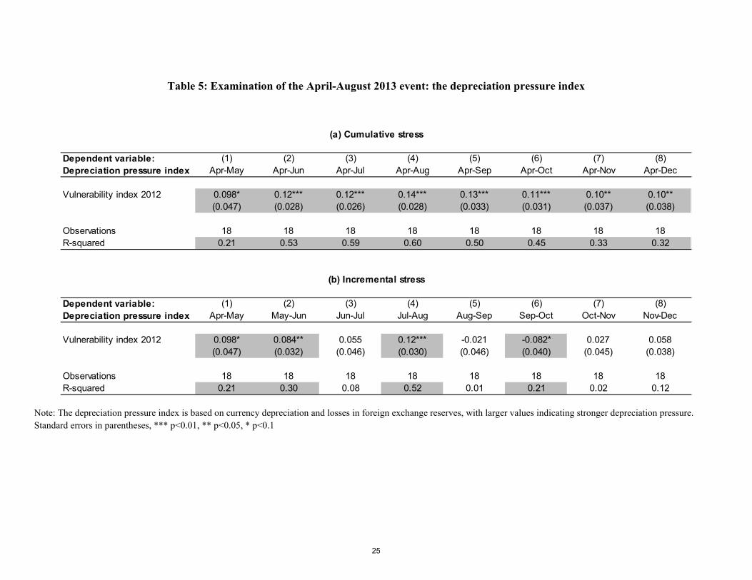
Table 5: Examination of the April-August 2013 event: the depreciation pressure index
Note: The depreciation pressure index is based on currency depreciation and losses in foreign exchange reserves, with larger values indicating stronger depreciation pressure. Standard errors in parentheses, *** p<0.01, ** p<0.05, * p<0.1
Dependent variable: (1) (2) (3) (4) (5) (6) (7) (8)Depreciation pressure index Apr-May Apr-Jun Apr-Jul Apr-Aug Apr-Sep Apr-Oct Apr-Nov Apr-Dec
Vulnerability index 2012 0.098* 0.12*** 0.12*** 0.14*** 0.13*** 0.11*** 0.10** 0.10**(0.047) (0.028) (0.026) (0.028) (0.033) (0.031) (0.037) (0.038)
Observations 18 18 18 18 18 18 18 18R-squared 0.21 0.53 0.59 0.60 0.50 0.45 0.33 0.32
Dependent variable: (1) (2) (3) (4) (5) (6) (7) (8)Depreciation pressure index Apr-May May-Jun Jun-Jul Jul-Aug Aug-Sep Sep-Oct Oct-Nov Nov-Dec
Vulnerability index 2012 0.098* 0.084** 0.055 0.12*** -0.021 -0.082* 0.027 0.058(0.047) (0.032) (0.046) (0.030) (0.046) (0.040) (0.045) (0.038)
Observations 18 18 18 18 18 18 18 18R-squared 0.21 0.30 0.08 0.52 0.01 0.21 0.02 0.12
(a) Cumulative stress
(b) Incremental stress
25

Table 6: Examination of the April-August 2013 event: the increase in bond yields
Note: Standard errors in parentheses, *** p<0.01, ** p<0.05, * p<0.1
Dependent variable: (1) (2) (3) (4) (5) (6) (7) (8)Increase in bond yields (ppt) Apr-May Apr-Jun Apr-Jul Apr-Aug Apr-Sep Apr-Oct Apr-Nov Apr-Dec
Vulnerability index 2012 -0.013 0.022 0.047* 0.072** 0.077** 0.062** 0.076*** 0.094***(0.011) (0.023) (0.025) (0.024) (0.028) (0.021) (0.023) (0.027)
Observations 14 14 14 14 13 13 14 14R-squared 0.11 0.07 0.22 0.44 0.40 0.44 0.47 0.50
Dependent variable: (1) (2) (3) (4) (5) (6) (7) (8)Increase in bond yields (ppt) Apr-May May-Jun Jun-Jul Jul-Aug Aug-Sep Sep-Oct Oct-Nov Nov-Dec
Vulnerability index 2012 -0.013 0.036* 0.025* 0.026*** 0.0059 -0.015 0.015 0.018**(0.011) (0.017) (0.013) (0.0073) (0.0070) (0.0093) (0.011) (0.0072)
Observations 14 15 15 15 14 14 14 15R-squared 0.11 0.25 0.22 0.50 0.06 0.18 0.13 0.32
(a) Cumulative stress
(b) Incremental stress
26

Table 7: Differentiation across EMEs during past events: the depreciation pressure index
Note: The depreciation pressure index is based on currency depreciation and changes in foreign exchange reserves, with larger values indicating stronger depreciation pressure. Standard errors in parentheses, *** p<0.01, ** p<0.05, * p<0.1
Dependent variable: (1) (2) (3) (4) (5) (6) (7)Depreciation pressure index Aug 1994 - Mar 1995 Jun 1997 - Jan 1998 Jul-Nov 1998 Mar-Oct 2002 Aug 2008 - Feb 2009 Jun-Dec 2011 Apr-Aug 2013
Vulnerability index (y-1) -0.0079 0.042 0.078 0.055 0.071** 0.097*** 0.14***(0.015) (0.043) (0.051) (0.043) (0.033) (0.026) (0.027)
Observations 18 15 19 18 19 20 20R-squared 0.02 0.07 0.12 0.09 0.21 0.43 0.61
Dependent variable: (1) (2) (3) (4) (5) (6) (7)Stock market change (%) Aug 1994 - Mar 1995 Jun 1997 - Jan 1998 Jul-Nov 1998 Mar-Oct 2002 Aug 2008 - Feb 2009 Jun-Dec 2011 Apr-Aug 2013
Vulnerability index (y-1) -2.13* -0.27 -0.67 -0.12 -0.25 -0.041 -0.074(1.07) (0.52) (1.11) (0.48) (0.36) (0.30) (0.27)
Observations 12 10 15 16 16 17 17R-squared 0.28 0.03 0.03 0.00 0.03 0.00 0.01
(a) Dependent variable: depreciation pressure index
(b) Dependent variable: stock market change (%)
27

Figure 1: Financial performance April-August 2013
Note: Exchange rates are expressed as units of local currency to the dollar, so that positive changes in exchange rates indicate depreciation. The depreciation pressure index is based on currency depreciation and losses in foreign exchange reserves, with larger values indicating stronger depreciation pressure. As an alternative, the depreciation pressure index 2 is based on currency depreciation, losses in foreign exchange reserves, and policy rate increases, with larger values indicating stronger depreciation pressure.
05
10Fr
eque
ncy
-10 0 10 20Exchange rate depreciation (%)
(1)
02
46
8Fr
eque
ncy
-30 -20 -10 0 10Change in FX reserves (%)
(2)
02
46
810
Freq
uenc
y
-2 -1 0 1 2Change in policy rate (ppt)
(3)
02
46
Freq
uenc
y
-1 0 1 2 3 4Depreciation pressure index
(4)
02
46
Freq
uenc
y0 2 4 6
Depreciation pressure index 2
(5)
01
23
Freq
uenc
y
0 .5 1 1.5 2 2.5Increase in LCY bond yields (ppt)
(6)
01
23
Freq
uenc
y
-20 -10 0 10Stock market price change (%)
(7)
01
23
4Fr
eque
ncy
-.5 0 .5 1Increase in EMBI spreads (ppt)
(8)
01
23
45
Freq
uenc
y
0 .2 .4 .6 .8 1Increase in CDS spreads (ppt)
(9)
28

Figure 2: Exchange rate depreciation and macroeconomic fundamentals during April-August 2013
Note: Exchange rates are expressed as units of local currency to the dollar, so that positive changes in exchange rates indicate depreciation.
th
ch
ru
ta
phco
mx mape
sfbz
pgar
ko
in
ug
pk
id
cl
tk
05
1015
2025
Exch
ange
rate
dep
reci
atio
n (%
)
-5 0 5 10CA/GDP (2012)
R-squared= 0.47
(1)
th
ch
ru
ta
phco
mx mape
sf
bz
pgar
ko
in
ug
pk
id
cl
tk
05
1015
2025
Exch
ange
rate
dep
reci
atio
n (%
)
0 20 40 60 80Reserves/GDP (2012)
R-squared= 0.20
(2)
th
ch
ru
ta
phco
mxmape
sf
bz
pgar
ko
in
ug
pk
id
cl
tk
05
1015
2025
Exch
ange
rate
dep
reci
atio
n (%
)
20 40 60 80 100ST debt/FX reserves (2012)
R-squared= 0.25
(3)
th
ch
ru
ta
phco
mx mape
sf
bz
pg ar
ko
in
ug
pk
id
cl
tk
05
1015
2025
Exch
ange
rate
dep
reci
atio
n (%
)
0 20 40 60 80Gross gov. debt/GDP (2012)
R-squared= 0.27
(4)
th
ch
ru
ta
phco
mxmape
sf
bz
pg ar
ko
in
ug
pk
id
cl
tk
05
1015
2025
Exch
ange
rate
dep
reci
atio
n (%
)
2 4 6 8 10 12Inflation, 3yma (2012)
R-squared= 0.23
(5)
th
ch
ru
ta
phco
mx mape
sf
bz
pgar
ko
in
ug
pk
id
cl
tk
05
1015
2025
Exch
ange
rate
dep
reci
atio
n (%
)
-10 0 10 20 30Credit/GDP runup (2012)
R-squared= 0.01
(6)
29

Figure 3: Increase in local currency government bond yields and macroeconomic fundamentals during April-August 2013
thch
ru
taph
co
mx
ma
sf
bz
koin
idtk
0.5
11.
52
2.5
Incr
ease
in L
CY
bond
yie
lds
(ppt
)
-5 0 5 10CA/GDP (2012)
R-squared= 0.45
(1)
thch
ru
taph
co
mx
ma
sf
bz
koin
idtk
-10
12
3In
crea
se in
LC
Y bo
nd y
ield
s (p
pt)
0 20 40 60 80Reserves/GDP (2012)
R-squared= 0.44
(2)
thch
ru
ta ph
co
mx
ma
sf
bz
koin
id tk
0.5
11.
52
2.5
Incr
ease
in L
CY
bond
yie
lds
(ppt
)
20 40 60 80 100ST debt/FX reserves (2012)
R-squared= 0.47
(3)
thch
ru
taph
co
mx
ma
sf
bz
koin
id tk
0.5
11.
52
2.5
Incr
ease
in L
CY
bond
yie
lds
(ppt
)
0 20 40 60 80Gross gov. debt/GDP (2012)
R-squared= 0.03
(4)
thch
ru
ta ph
co
mx
ma
sf
bz
koin
id tk
0.5
11.
52
2.5
Incr
ease
in L
CY
bond
yie
lds
(ppt
)
2 4 6 8 10 12Inflation, 3yma (2012)
R-squared= 0.11
(5)
thch
ru
taph
co
mx
ma
sf
bz
koin
id tk
0.5
11.
52
2.5
Incr
ease
in L
CY
bond
yie
lds
(ppt
)
-10 0 10 20 30Credit/GDP runup (2012)
R-squared= 0.00
(6)
30

Figure 4: Identification of past events of financial stress
Note: The start and end dates for each of the 13 events in chronological order are as follows: (1) August 3 to November 9, 1990; (2) September 16, 1994 to March 10, 1995; (3) July 4 to August 29, 1997 and October 31, 1997 to January 9, 1998, merged in one single event; (4) August 7 to November 13, 1998; (5) July 14 to December 22, 2000; (6) April 19 to October 11, 2002; (7) July 20 to August 17, 2007; (8) October 26, 2007 to March 21, 2008; (9) September 12, 2008 to February 27, 2009; (10) April 16 to May 28, 2010; (11) July 29 to December 16, 2011; (12) March 2 to June 8, 2012; and (13) May 10 to August 30, 2013.
31

Figure 5: Depreciation pressure and economic fundamentals during past events of financial stress
Note: For each event, the vertical axis shows the depreciation pressure index (based on currency depreciation and losses in foreign exchange reserves), with larger values indicating stronger depreciation pressure.
th
ch
ta
phcoma
pe
sf
bz
pg
ar
koin
ug
pk
id
cl tk
-1-.5
0.5
10 15 20 25 30Vulnerability index (1993)R-sq = 0.02 exludes MX
(1) Aug 1994 - Mar 1995
ch
ru
ta co
mx
pe sf
bz
pg
ar
in
ug
pk
cl
tk
-10
12
3
10 15 20 25 30Vulnerability index (1996)
R-sq = 0.07 ex. ID KO MA PH TH
(2) Jun 1997 - Jan 1998
th
chta
ph
comx
ma
pe
sf
bz
pgar
koin
ug
pk
id
cl
tk
-2-1
01
23
10 15 20 25 30Vulnerability index (1997)
R-sq = 0.12 excludes RU
(3) Jul - Nov 1998
th chruta
phco
mxma pe
sf
bz
pg
ko in
pk
idcl tk
-4-2
02
4
10 15 20 25 30Vulnerability index (2001)
R-sq = 0.09 excludes AR UG
(4) Mar - Oct 2002
thch
ta ph
co
mx
ma
pe
sf
bz
pg
ar
ko
in
ug
pk
id
cl
tk
01
23
0 10 20 30 40Vulnerability index (2007)R-sq = 0.21 excludes RU
(5) Aug 2008 - Feb 2009
th
ch
ru
ta
ph
comx
ma
pe
sf
bz
pgarko
in
ug
pkid
cl
tk
-10
12
34
10 20 30 40Vulnerability index (2010)
R-sq = 0.43
(6) Jun - Dec 2011
th
ch
ru
ta
ph
co
mxma
pe
sfbz
pg
ar
ko
in
ug
pkid
cl
tk
01
23
4
10 15 20 25 30 35Vulnerability index (2012)
R-sq = 0.61
(7) Apr - Aug 2013
32

Figure 6: Stock market declines and economic fundamentals during past events of financial stress
Note: For each event, the vertical axis shows the percentage change in the local stock market index.
thch
ta
ph
ma
pe
bzar
ko
in
id
cl
-40
-30
-20
-10
010
10 15 20 25 30Vulnerability index (1993)R-sq = 0.28 exludes MX TK
(1) Aug 1994 - Mar 1995
ch
ru
ta
mx
pe
sfbz
ar
in
cl-20
-10
010
10 15 20 25 30Vulnerability index (1996)
R-sq = 0.03 ex. ID KO MA PH TH TK
(2) Jun 1997 - Jan 1998
th
chta
ph
mx
ma
pesfbzar
ko
in
id
cl
tk-40
-20
020
40
10 15 20 25 30Vulnerability index (1997)
R-sq = 0.03 excludes RU
(3) Jul - Nov 1998
thch
ru
taph
co
mxma
pesf
bz
ko
inid
cl tk
-40
-20
020
10 15 20 25 30Vulnerability index (2001)
R-sq = 0.00 excludes AR UG
(4) Mar - Oct 2002
th
ch
ta
ph
co
mx
ma
pe
sfbz
ar
ko
inid
cl
tk
-50
-40
-30
-20
-10
0 10 20 30 40Vulnerability index (2007)R-sq = 0.03 excludes RU
(5) Aug 2008 - Feb 2009
th
ch
ruta
ph
co
mx
mape
sf
bz
ar
koin
id
cl
tk
-30
-20
-10
010
10 20 30 40Vulnerability index (2010)
R-sq = 0.00
(6) Jun - Dec 2011
th
chru
ta
ph
co
mx
ma
pe
sf
bz
ar
koin
idcl
tk-15
-10
-50
510
10 15 20 25 30 35Vulnerability index (2012)
R-sq = 0.01
(7) Apr - Aug 2013
33