interval inversion approach for an improved interpretation

1

Interval inversion approach for an improved interpretation of well logs

Mihály Dobróka1, Norbert Péter Szabó1,2, József Tóth3, Péter Vass3

Right running head: Interval inversion of well logs

1University of Miskolc, Department of Geophysics, Miskolc,

Hungary.

2MTA-ME, Geoengineering Research Group, Miskolc, Hungary

3MOL Hungarian Oil and Gas Plc., Petrophysical Department,

Szolnok, Hungary

E-mail: [email protected], [email protected],

[email protected], [email protected]

Date of submission: 28 November 2015

of 61 Geophysics Manuscript, Accepted Pending: For Review Not Production

2

ABSTRACT

The quality analysis of well-logging inversion results has always

been an important part of formation evaluation. The precise

calculation of hydrocarbon reserves requires the most possible

accurate estimation of porosity, water saturation, and shale and rock-

matrix volumes. The local inversion method conventionally used to

predict the above model parameters depth-by-depth represents a

marginally overdetermined inverse problem, which is rather sensitive

to the uncertainty of observed data and limited in estimation accuracy.

To reduce the harmful effect of data noise on the estimated model we

suggest the interval inversion method, in which an increase of the

overdetermination ratio allows a more accurate solution of the well-

logging inverse problem. The interval inversion method inverts the

data set of a longer depth-interval to predict the vertical distributions

of petrophysical parameters in a joint inversion procedure. In

formulating the forward problem, we extend the validity of probe

response functions to a greater depth-interval assuming the

petrophysical parameters depth-dependent, and then we expand the

model parameters into series by using Legendre polynomials as basis

functions for modeling inhomogeneous formations. We solve the

inverse problem for much smaller number of expansion coefficients

than data to derive the petrophysical parameters in a stable

overdetermined inversion procedure. The added advantage of the

of 61Geophysics Manuscript, Accepted Pending: For Review Not Production

3

interval inversion method is that the layer-thicknesses and suitably

chosen zone parameters can be estimated automatically by the

inversion procedure to refine the results of both inverse and forward

modeling. We define depth-dependent model covariance and

correlation matrices to compare the quality of the local and interval

inversion results. A detailed study using well logs measured from a

Hungarian gas-bearing unconsolidated formation demonstrates that

the greatly overdetermined interval inversion procedure can be

effectively used in reducing the estimation errors in shaly sand

formations, which may refine significantly the results of reserve

calculation.

INTRODUCTION

In oilfield practice, we utilize open-hole logging data to determine

essential petrophysical parameters of geological formations that

underlie the calculation of hydrocarbon reserves. Some of the

reservoir parameters such as effective porosity, water saturation, shale

content and fractional volume of rock matrices can be determined with

their estimation errors from the joint inversion of suitable well logs. In

well log analysis, we assume known mathematical relations, called

probe response functions, between the observations and the

petrophysical model to predict data with the actual model. In the

inversion procedure, one gives an estimate to the model parameters by


4

fitting theoretical data to the measured data. An excellent overview on

the theory and computer implementation of well-logging inversion

methods are given in Mayer and Sibbit (1980), Alberty and Hashmy

(1984) and Ball et al. (1987).

Commercial inversion techniques routinely used in formation

evaluation simultaneously process all the data collected with different

probes from a certain depth to determine the petrophysical properties

of reservoir rocks to the same depth. In shaly sand analysis, we

usually have barely more types of probes than the number of

unknowns in a given depth, thus we have to solve a set of marginally

overdetermined inverse problems along a borehole. Although the local

inversion method gives fast and satisfactory results, its narrow

overdetermination (data-to-unknowns ratio) sets a limit to estimation

accuracy, which makes it a relatively noise-sensitive inversion

procedure. The quality of estimation results can be improved by

increasing the amount of observed information using more types of

well logs, which has well-known technological limits. There is

another possibility to improve the accuracy of inversion estimates. We

suggest increasing the overdetermination ratio of the inversion

procedure by inverting the data set of a longer processing interval in a

joint inversion procedure. Dobróka and Szabó (2001) introduced the

interval inversion method that uses depth-dependent response

functions (instead of local ones) in solving the forward problem. In the


5

phase of inversion, we use a series expansion-based model

discretization technique and invert at least an order (or orders) of

magnitude higher number of data than unknowns compared to local

inversion. The utilization of our inversion strategy bears great

influence on the accuracy and reliability of model parameters

extracted by inversion. Heidari et al. (2012) also emphasized the

importance of inverting a data set collected from more depths jointly

to improve the efficiency of well log interpretation.

Model discretization by means of series expansion is extensively

used in natural and technical sciences, including geophysical research.

In geoelectric data processing, the series expansion-based inversion

methodology was used to evaluate the 2D resistivity and thickness

distribution of shallow structures and an optimization method was

suggested for giving the optimal number of inversion unknowns

(Gyulai and Ormos, 1999). They showed significant improvement in

reducing the estimation errors and ambiguity. They also increased the

lateral resolution without using any smoothness constraint. This

geoelectric inversion algorithm was further developed for 3D

applications by Gyulai and Tolnai (2012). A series expansion-based

joint inversion method for the interpretation of DC geoelectric and

seismic refraction data measured above 2D geologic structures was

introduced by Kis (2002). In gravity modeling, the series expansion

approach opened the door to reconstruct the 3D potential function and


6

the full Eötvös-tensor from a large number of astronomical, torsional

pendulum and gravity data by solving a greatly overdetermined

inverse problem (Dobróka and Völgyesi, 2008). Turai (2011) gave an

estimate to the relaxation time spectrum by using a series expansion-

based inversion of induced polarization data. Dobróka et al. (2015)

published a series expansion-based Fourier transformation method in

which the Fourier spectrum was developed in the framework of a

significantly overdetermined inverse problem characterized by highly

improved noise rejection capability.

The series expansion-based interval inversion method developed

for well log analysis has been previously used to estimate the

petrophysical parameters and thicknesses of homogeneous layers. To

find the global minimum of misfit between observed and predicted

data a Simulated Annealing (SA) optimization procedure was

implemented, which showed considerable improvement in the

suppression of data noise compared to local inversion procedures. The

layer-thicknesses cannot be extracted by any local inversion method,

because neither the local response functions include them explicitly

nor the data measured at a given depth contain information on the

position of distant layer boundaries. However, the basis functions of

series expansion can be chosen as depending on the boundary

coordinates, which allows the interval inversion procedure to estimate

them automatically (Dobróka and Szabó, 2001). In addition, the lateral


7

variation of formation boundaries along a profile of boreholes together

with petrophysical parameters were determined from a 2D interval

inversion procedure by Dobróka et al. (2009). An oilfield application

for the estimation of layer-thicknesses using a Float-Encoded Genetic

Algorithm was shown in Dobróka and Szabó (2012). Since the

interval inversion method allows treating increasing number of

unknowns without the significant decrease of overdetermination, one

can estimate additional unknowns of interest. As a new feature of the

interval inversion method, the simultaneous determination of

conventional petrophysical (volumetric) properties and textural

parameters, i.e. cementation exponent, saturation exponent and

tortuosity factor, was suggested by Dobróka and Szabó (2011), while

the evaluation of carbonate and metamorphic reservoirs was shown in

Dobróka et al. (2012).

The advantages of the interval inversion method using a

homogeneous layer approximation are represented by the optimal

overdetermination ratio, accurate and reliable solution, effective noise-

suppression feature and automatic estimation of layer-thicknesses.

However, we find also some practical drawbacks, for instance, if we

neglect the lithological variations within inhomogeneous layers, we

obtain only a rough estimation result typically indicated by high level

of misfit between the predicted and observed data. As a consequence,

the layer-wise homogeneous approximation can result in poor vertical


8

resolution in the evaluation of inhomogeneous formations. In this

study, we introduce a further developed interval inversion method

using a Legendre polynomial-based discretization technique to

increase the vertical resolution in inhomogeneous hydrocarbon-

bearing formations. The use of the orthogonal set of basis functions

decreases the data misfit compared to layer-by-layer inversion and

assures reduced correlation between the model parameters. Largely

increased overdetermination of the inverse problem results in a highly

accurate estimation of the petrophysical model, while the utilization of

linear optimization provides a quick and steady convergence to the

optimum. We compare the conventionally used local inversion

procedure to the interval inversion method in a detailed study using

real well-logging data. We show that the latter provides a significant

improvement in the accuracy and reliability of inversion estimates,

which has unequivocal practical benefits in the calculation of

hydrocarbon reserves.

THEORETICAL OVERVIEW

Local inversion method

Let d(obs) be an S-by-1 vector of well-logging data observed by

different probes in a certain depth and m be an P-by-1 vector of model

parameters defined in the same depth. The former includes various

nuclear, acoustic and electric logs, while the latter incorporates the


9

volumetric ratios of rock constituents as unknowns of the local inverse

problem. In forward modeling the s-th data is calculated as

( ) ( )c,,,, 21 Ps

cal

s mmmgd K= , (1)

where gs represents the local response function of the s-th logging tool

(s=1,…,S) and S is the total number of probes. In the general case, the

set of probe response functions is nonlinear, which may depend on all

model parameters (m) and a set of zone parameters (c) including the

physical (well log) properties of pore-fluids and mineral components

unvarying or just slowly varying in the hydrocarbon zone. By treating

the zone parameters as known constant, we solve a marginally

overdetermined inverse problem in shaly sands, where the number of

data is barely more than that of the model parameters. We write the

linear approximation of equation 1 in a subscripted form as

( ) ∑=

=P

i

isi

cal

s mGd1

, (2)

where ( )0missi mgG ∂∂= is the element of the Jacobi’s matrix

calculated in the m0 point of the parameter space continuously

improved during an iteration procedure. The objective function of the

inverse problem to be minimized is

2

2

22

2me ε+=E , (3)


10

where e denotes the S-by-1 vector of deviations between the observed

and calculated data normalized to the uncertainty of data ε is a

regularization parameter used for numerically stabilizing the solution

of the inverse problem. If we do not have prior information on data

variances, the residual errors can be weighted by the measured data to

control the relative importance of each well log in the inversion

procedure. The minimization can be solved by using a linearized

(Menke, 1984) or a global optimization method (without linearization)

such as Very Fast Simulated Annealing (Sen and Stoffa, 2013) or

Float-Encoded Genetic Algorithm (Michalewicz, 1996).

Interval inversion method

The interval inversion method is based on the establishment of

depth-dependent probe response functions. In the forward modeling

phase of the inversion procedure, we calculate the s-th well log using

equation 1 extended to a greater depth interval

( ) ( )( ) ( ) ( ) ( )( )rPrrsr

calcal

r zmzmzmgzdd ,,, 21 K== , (4)

where zr is the coordinate of the r-th depth (r=1,…,Ns) and Ns is the

number of the measurement points of the s-th well log. The above

formulation allows for integrating all the data collected from an

arbitrary interval to a joint inversion procedure. To do this we

introduce the integrated data vector


11

( ) [ ]T

1111

1 ,...,,...,,...,,...,,...,1

S

N

Ss

N

s

N

cal

Ssdddddd=d , (5)

where T denotes the symbol of matrix transpose. The k-th element of

the calculated data vector can be identified as

121 ... −++++= sNNNrk , where index r runs through the data set

belonging to the s-th well log. The total number of data is

SNNNN +++= ...21 . The k-th calculated data is approximated in a

linearized form as

( ) ∑=

=P

i

iki

cal

k mGd1

. (6)

In equation 4, the petrophysical parameters are represented as

continuous depth functions, while the zone parameters neglected from

the argument are fixed, but if necessary, they can be treated as depth-

dependent quantities, too. We discretize the i-th model parameter by

using a series expansion technique

( ) ( )∑=

=)(

1

iQ

q

q

(i)

qi zΨBzm , (7)

where Bq is the q-th expansion coefficient, Ψq is the q-th basis

function, Q(i) is the requisite number of expansion coefficients

(defined later) in describing the i-th model parameter. The basis

functions are assumed as known quantities the selection of which is


12

not strictly limited. In describing a layer-wise homogeneous model we

use a combination of unit step functions

( ) ( ) ( )qqq ZzuZzuzΨ −−−= −1 , (8)

where Zq-1 and Zq are the upper and lower depth-coordinates of the q-th

layer, respectively. Basis function Ψq in the q-th layer equals to unity,

otherwise it is zero, thus the i-th model parameter in the q-th layer can

be described by one expansion coefficient ( )(i

qB ). The advantage of

this formulation is the high overdetermination of the inverse problem.

Moreover, the layer-boundary coordinates appearing in equations 6−8

can be automatically estimated by the interval inversion method

(Dobróka and Szabó, 2012).

In this study, we approximate the variation of petrophysical

parameters by using Legendre polynomials as basis functions

( ) ( )∑=

−=)(

11

iQ

q

q

(i)

qi zPBzm , (9)

where the q-th degree Legendre polynomial can be written by using

the Rodrigues’ formula (McCarthy et al., 1993)

( ) ( )q

q

q

qq zzq

zP 1d

d

!2

1 2 −= . (10)


13

The Legendre polynomials form an orthonormal set of functions over

the range of −1 and 1. In the selection of Q one should tend to reduce

the number of expansion coefficients to guarantee the numerical

stability of the inversion procedure, while the proper vertical

resolution of petrophysical parameters requires sufficient number of

expansion coefficients. By substituting equation 9 to equation 4 the s-

th well log can be expressed in terms of the expansion coefficients.

The petrophysical parameters no longer constitute the model vector of

the inverse problem, instead of them, the expansion coefficients are

estimated directly by the inversion procedure. The application of

Legendre polynomials is favorable because of the relatively low

correlation developing between the model parameters during the

inversion process. When we give an estimate to the layer-thicknesses

by the interval inversion method the choice of a global optimization

algorithm is preferable to avoid numerical problems pertaining to

linearization (Dobróka and Szabó, 2011; Dobróka and Szabó, 2012).

According to our tests, assuming given layer-thicknesses the

linearized Damped Least Squares (DLSQ) method, suggested by

Marquardt (1959), produces a highly stable and fast interval inversion

procedure. By combining equations 6 and 7 we find

( ) ( ) ( ) ( )∑∑= =

==P

i

Q

q

kq

(i)

qkikk

i

zΨBGzdd1 1

calcal

)(

. (11)


14

Having two indices instead of (i)

qB we introduce lB as the l-th element

of the model vector of the interval inversion problem, where

121 ... −++++= iQQQql . The total number of unknowns is

PQQQM +++= ...21 . By replacing the term ( )kqki zΨG with klG~

, we

write the k-th calculated data as

( ) ∑=

=M

l

lkl

cal

k BGd1

~. (12)

Depth-coordinate zk and indices q and i belonging to l can be

determined by the above re-parametrization. The linearized inverse

problem can be solved by minimizing the functional given in equation

3. The M-by-1 vector of expansion coefficients is estimated as

)(obsgdGB

−= , (13)

where G-g is the generalized inverse matrix of the DLSQ method

(Menke 1984). The vertical distribution of petrophysical parameters

can be derived directly from the interval inversion results using

equation 9.

Quality of inversion results

We check the quality of inversion estimates in the knowledge of

the accuracy of input data, which can be provided by repeated well-

logging measurements or operation manuals. Horváth (1973)


15

discussed the sources of interpretation errors and gave an estimate to

the uncertainty of different types of well-logging data. In the general

case, the covariance matrix of the model parameters estimated by a

linearized inversion method can be related to the data covariance

matrix including the variances of observed data in its main diagonal

(Menke, 1984)

( ) ( )Tcovcov -gobs-g GdGm = . (14)

The dispersion of model parameters is not only the result of data

noise, but is also affected by some amount of modeling errors related

to equation 1. The estimation error of the i-th model parameter is

derived from equation 14

( ) ( )[ ] 2/1coviiim m=σ , (15)

which we use to measure the accuracy of the model parameters

estimated by local inversion. One can calculate the covariance matrix

of the expansion coefficients (covB) estimated by the interval

inversion procedure by analogy with equation 14, where the variance

of each datum available in the processing interval is included in the

data covariance matrix. The calculation of the accuracy of

petrophysical parameters derived from equation 9 requires the

propagation of errors taken into consideration. In the knowledge of


16

Bcov , we derive the covariance between the petrophysical

parameters mi and mj at an arbitrary depth as

( )[ ] ( )( ) ( )zΨzΨz m

Q

n

Q

m

ni

i j

∑∑= =

′=)( )(

1 1hhj covcov Bm , (16)

where indices are h=n+Q1+Q2+…+Qi-1, h’=m+Q1+Q2+…+Qj-1

(i=1,2,…,P and j=1,2,…,P). When applying Legendre polynomials of

different degrees as basis functions, equation 9 derives that

( ) ( )zPB/zm 1-q

(i)

qi =∂∂ which substituted into equation 16 gives

( )[ ] ( )( ) ( )zPzPz m

Q

n

Q

m

hhnji

i j

11 1

1

)( )(

covcov −= =

′−∑∑= Bm . (17)

Analogously to equation 15 the estimation error is derived from

equation 17, which gives the standard deviation of the i-th

petrophysical parameter estimated by the interval inversion procedure

in the function of logged depth for either correlated or uncorrelated

measurements.

The reliability of inversion results can be quantified via the

Pearson’s correlation matrix (corr m). We consider a solution reliable

when the model parameters correlate marginally, because only

uncorrelated (or just poorly correlated) parameters can be resolved

uniquely by inversion. If the absolute value of correlation coefficient

is close to unity, there is a strong relation between the model


17

parameters referring to unreliable solution. In large-scale inverse

problems, it is useful to introduce a scalar for the measure of average

correlation

( )( )

( )[ ]21

P

1i

P

1j

2ijδcorr

1-PP

1S

/

ij

−= ∑∑= =

mm , (18)

where δ denotes the Kronecker delta. The above quantity refers to the

case of local inversion, which can be extended for checking the

reliability of interval inversion results. We define the correlation

matrix of expansion coefficients estimated to the entire processing

interval as

( ) ( )( ) ( )ll

llll BσBσ

covcorr

′

′′ =

BB , (19)

where indices are l=1,2,…,M, l’=1,2,…,M and M is the total number

of expansion coefficients estimated by the polynomial-based interval

inversion method. The correlation matrix of vector B can be

represented similarly by the scalar defined in equation 18. We

quantify the overall misfit between the measured and predicted data of

different magnitudes and dimensional units by the relative data

distance

( )%1001

2/1

1

2

)(

)()(

⋅

−= ∑

=

N

kobs

k

cal

k

obs

k

d

dd

ND , (20)


18

where )()( and cal

k

obs

k dd are the k-th element of the observed and

calculated (integrated) data vector, respectively.

FIELD RESULTS

Inverse problem

We test the interval inversion method and compare it to local

inversion in a hydrocarbon exploratory borehole (Well-1) drilled in

the Pannonian Basin in Hungary. In the processed interval a

sedimentary formation of Upper Pannonian (Pliocene) made up of

four unconsolidated layers are investigated. Rock samples indicates

high porosity channel sands of good storage capacity interbedded by

aleurite laminae and shaly layers. Well-logging data suitable for

inversion are represented by natural gamma ray (GR in API), spectral

(potassium) gamma ray (K in %), bulk density (ρb in g/cm3), neutron

porosity (ΦN in v/v), acoustic traveltime (∆t in µs/ft) and deep

laterolog resistivity (Rd in ohm-m) logs. The depth-matched and

environmentally corrected well logs transformed into the depth

interval of 0−19.3 m are plotted in Figure 1. In the last track, the

combination of density and neutron logs indicates the presence of

hydrocarbons in the second and fourth layers. The pore-fluid was

identified previously as methane, ethane, propane and a small amount

of carbon dioxide. In the lack of observed information on data


19

variances, we assume that the well logs are of different uncertainties.

We give the data covariance matrix in equation 14

( ) ( )222222 ,,,,,diagcovdNb R∆tΦρKGR

obs σσσσσσ=d . (21)

For studying the effect of data variance on the solution of the inverse

problem we estimate the standard deviations of data, similarly to

Horváth (1973), as 08.0=σGR , 07.0=σK , 05.0=σbρ

, 09.0=σNΦ

,

06.0=σ∆t , 06.0=σdR . The confidence intervals of well logs

measured in Well-1 are indicated in Figure 1.

The general form of the k-th probe response equation is

( )c,0 sdshwxk ,V,V,SΦ,Sfd = , (22)

where effective porosity Φ (v/v), shale volume Vsh (v/v), sand volume

Vsd (v/v), water saturation in the invaded Sx0 (v/v) and that of

uninvaded zone Sw (v/v) are the unknowns of the inverse problem. To

simulate nuclear logs (GR, K, ρb, ΦN) linear response functions

corrected for shale, mudfiltrate and hydrocarbon effects are employed

suggested for shaly sand interpretation by Baker Atlas (1996). For

calculating the sonic response (∆t) the compaction corrected time-

average formula is applied (Wyllie et al. 1956). Deep resistivity (Rd)

log is calculated first by different nonlinear models, i.e. Archie

formula (Archie 1942), Simandoux equation (Simandoux 1963), total


20

shale relationship (Schlumberger 1989) and Indonesia model (Poupon

and Leveaux 1971). By solving the interval inversion problems

separately, the overall data distance based on equation 20 (calculated

only for resistivity data) is 2.8 % for the Archie equation, 3.4 % for

the Indonesia model, 2.6 % for the Schlumberger model and 4.4 % for

the Simandoux model. Since it gives the lowest misfit, we choose the

total shale model for testing the local and interval inversion procedure.

In equation 22, the zone parameters in vector c representing the

physical properties of mud filtrate, hydrocarbon, shale and sand are

treated as constant in the local inverse problem (Table 1). They can be

estimated from literature, drilling information, core measurements,

crossplot techniques, trial-and-error method or some of them

alternatively by interval inversion (Dobróka and Szabó, 2011). The

material balance equation used to constrain the estimation of

petrophysical parameters is 1=++ sdsh VVΦ . Equation 22 does not

contain the layer-boundary coordinates, which cannot be extracted by

local inversion methods. They can be a priori given from manual

analysis of the GR or shallow resistivity logs, determined by

multivariate statistical methods, such as cluster analysis, fuzzy logic

and neural networks (Maiti et al., 2007), or estimated automatically by

interval inversion (Dobróka and Szabó, 2012).

In solving the inverse problem, we apply two different approaches.

The traditional is represented by the local inversion method, which


21

extracts the petrophysical parameters depth-by-depth with the

subsequent analysis of local data sets. On the contrary, the interval

inversion method integrates all the data collected from the logged

interval to produce the well logs of petrophysical parameters in a joint

inversion procedure. The discretization of model parameters is made

by equation 9, which can be applied to an arbitrary depth interval. We

suggest specifying the depth interval of series expansion

automatically by using a more sophisticated interval inversion

algorithm. In the first phase, an interval inversion problem is solved

using equation 8 to give an estimate to layer-thicknesses and

petrophysical parameters of a homogeneous layer model using the SA

method. We choose equation 3 as energy function extended to the

entire processing interval. The following cooling schedule assures to

achieve the global optimum (Geman and Geman, 1984)

( )( )ν

νln

0TT = , (23)

where T0 denotes an appropriate initial temperature, ν is the number

of iteration steps. At the end of the SA procedure, we separate

different layers in which the estimated constants of petrophysical

parameters can be considered as initial values of expansion

coefficients of Legendre polynomials of the zeroth order in equation

9. In the second phase, we refine the vertical distributions of


22

petrophysical parameters within the separated intervals in distinct

interval inversion procedures using Legendre polynomials as basis

functions. For this purpose, we perform a DLSQ-based interval

inversion of well logs to give a fast and stable solution.

In inversion procedures analyzed in this study, we use the same

forward problem solution. We show that the set of response equations

applied in this study gives a proper fit between measured and

calculated data in Well-1. In case of more complex geological

situations the forward modeling equations can be further developed,

e.g. by Drahos (1984), Tang and Cheng (1993) and Mendoza et al.

(2010), which can be easily implemented in the interval inversion

procedure. In this study, we lay emphasis on the improvement of the

inversion algorithm. Our aim is to develop a powerful inversion tool,

which provides better estimation accuracy than local inversion

procedures. This is attained by the significant increase of

overdetermination using a Legendre polynomial-based discretization

strategy. Therewith, the treatment of zone parameters as inversion

unknown can be considered as a step-forward in the forward problem

solution, too. In our conception, it is a petrophysics-based innovation

that we give an objective estimate to zone parameters instead of fixing

them arbitrarily during the inversion procedure.

Comparative study


23

We compare the polynomial series expansion-based interval

inversion method to the local inversion procedure. The aim of the

present task is to determine the vertical distributions of quantities Φ,

Sx0, Sw, Vsh, Vsd in Well-1. Since we have six types of data in each

depth (GR, K, ρb, ΦN, ∆t, Rd) and we can estimate the sand volume

deterministically from the material balance equation, the

overdetermination ratio in case of depth-by-depth inversion is 1.5.

(We have 4 unknowns in each depth, totally 776 unknowns in the

investigated interval.) In local inversion, we first set an initial model

by giving a first guess to the model parameters. In permeable layers

we assume the starting values of Φ=Sw=Vsh=0.2 v/v, Sx0=0.7 v/v, while

in impermeable beds we set them as Φ=0.1 v/v, Sx0=Sw=1.0 v/v,

Vsh=0.6 v/v. We do not allow the water saturation to exceed unity. We

use the DLSQ algorithm to solve the local inverse problem. Since the

condition number of matrix GTG derived from equation 2 is

occasionally 2·103−1.2·104, we choose the regularization factor ε2 in

equation 3 as 15, which we decrease progressively down to 3·10-5 in

10 iteration steps. We calculate the data distance defined in equation

20 to each depth the average of which is 3.7 % at the end of the

inversion procedure. The CPU time of the inversion process is 11 s

using a quad-core processor workstation. The local inversion results

are illustrated in Figure 2. Tracks 1−6 show a close fit between the

observed and calculated data. The well logs of the estimated


24

petrophysical parameters are in tracks 7−8. In the saturation track, the

movable and irreducible hydrocarbon saturations are derived from the

inversion results by Shm=Sx0−Sw and Shir=1−Sx0, respectively. The

fractions of porosity (Φ=0.04−0.28 v/v), shale (Vsh=0.08−0.71 v/v),

sand (Vsd=0.21−0.69 v/v) relative to the unit volume of rock are

plotted in track 8.

In the next step, we estimate the distribution of petrophysical

parameters in the entire logging interval by the DLSQ-based interval

inversion procedure. By a sampling distance of 0.1 m, we have totally

1,164 datum. We discretize the model parameters (Φ, Sx0, Sw, Vsh) by

using equation 9 with applying a set of Legendre polynomials of

degree up to 44 as basis functions. (The optimal choice of polynomial

degree will be discussed two subsections later.) The total number of

unknowns is 4(Q*+1)=180 (Q* is the maximum degree of the

Legendre polynomials), thus the data-to-unknowns ratio is 6.5. The

relative increase in overdetermination ratio is over 330% compared to

local inversion. We choose the initial values of expansion coefficients

as B1=0.1 for Φ, B1=0.5 for Sx0, B1=0.2 for Sw and Vsh, respectively,

while Bq=0 (q=2,3,…,45) is applied to every petrophysical parameter.

We calculate the 1164×180 Jacobi’s matrix in each iteration step,

while the condition number of the 180×180 matrix GTG is around

300. Thus, we do not have to apply the regularization term in equation


25

3 and the inversion procedure is still stable at ε2=0. We set the

maximum number of iteration steps to 10. The data distance is 728 %

in the first step, which decreases down to 4.4 % after six iteration

steps. The CPU time of the inversion process is 1 min 56 s using the

same workstation. The relative increase of processing time is 9.5

compared to local inversion. The expansion coefficients with their

estimation errors calculated by equation 16 are illustrated in Figure 3.

The relative errors of coefficient B1 is 3−6 %. The standard deviation

of porosity and shale content is smaller than that of the water

saturation. The 180×180 correlation matrix of expansion coefficients

calculated by equation 19 is illustrated in Figure 4c, while the 4×4

correlation matrices of model parameters estimated by local inversion

in an impermeable layer (z=2 m) and in a permeable bed (z=12 m) are

plotted in Figure 4a−b, successively. The correlation average defined

in equation 18 shows that the strength of correlation between the

model parameters is much smaller for interval inversion, i.e. the

relative decrease in the average of absolute values of correlation

coefficients is 70 %, which refers to a more reliable estimation for the

inversion unknowns. The small value of correlation average explains

the great stability of the interval inversion procedure. The result of

well log analysis is illustrated in Figure 5. The calculated well logs are

in close agreement with the observed ones (tracks 1−6). The variation

of water saturation along the borehole is somewhat smoother


26

compared to the case of local inversion (track 7). The relative volumes

of porosity (Φ=0.03−0.28 v/v), shale (Vsh=0.07−0.71 v/v) and sand

(Vsd=0.24−0.69 v/v) are plotted in track 8.

The estimation errors of petrophysical parameters can be compared

in Figure 6, which are calculated by equation 15. The standard

deviation of water saturation is one order of magnitude higher than

that of the porosity and shale volume. In permeable layers, the

estimation errors are relatively small, but in impermeable beds, they

abruptly increase because of the stronger correlation between the

model parameters. In tracks 6−7, the high values of correlation

averages with small data distances indicate an ambiguous

interpretation of water saturation in shaly intervals, which makes the

estimation error of petrophysical parameters locally increase. The

overall result shows that the interval inversion procedure improves the

estimation accuracy compared to the local inversion method. We

achieve 60 % relative decrease in the average standard deviation of

porosity, 52 % in that of water saturation in the uninvaded zone, 55 %

in that of shale content, 50 % in that of water saturation in the invaded

zone. The improvement is well marked in impermeable intervals,

while the use of the interval inversion method is the most favorable in

hydrocarbon reservoirs, where the absolute value of estimation error is

the smallest. The improvement of estimation accuracy for porosity and

water saturations in the fourth layer is demonstrated in Figure 7. The


27

correlation coefficients for petrophysical parameters estimated by

local inversion can be compared to those of the interval inversion

results in Figure 8. The overall strength of correlation between the

volumetric parameters is weaker in case of interval inversion. The

improvement is more significant in shaly layers than in the

hydrocarbon reservoirs. The average correlation between the

petrophysical parameters is 0.44 for interval inversion, which means a

relative decrease of 12 % as opposed to local inversion. Almost an

entire correlation between porosity and water saturation causes the

large estimation errors in the first and third layers. The water

saturations of the invaded and virgin zone are also strongly correlated

to each other. In these cases, one of them should be estimated out of

the inversion procedure. Figure 9 demonstrates a good correlation

between the porosities estimated independently by the interval

inversion procedure, CLASS deterministic approach (Baker Atlas

1996) and core data available from neighboring boreholes (Well−2 is

located ~1300 m, while Well−3 is ~500 m away from Well−1). The

hydrocarbon formation correlate well between the boreholes and the

interval inversion results show close fit to those of the independent

evaluation procedures. As a conclusion, the interval inversion method

gives more accurate and reliable estimation in a more stable inversion

procedure compared to local inversion. In the presented case, the

interval inversion method gives a smoother but more accurate solution


28

with slightly worse data misfit. The vertical resolution depends on the

selection of the number of unknowns of the inverse problem.

Determination of interval length

The major increase of the number of expansion coefficients in the

same depth-interval can improve the vertical resolution of the interval

inversion method, but it may also lead to the large-scale decrease of

overdetermination and estimation accuracy. One can enlarge the

resolution capability of the interval inversion method also with

separating the processed length into smaller intervals in which one can

expand the petrophysical parameters into series with sufficient number

of expansion coefficients.

We execute the SA-based interval inversion procedure using the

discretization scheme 8 as a preliminary data processing step to

separate different lithological units and designate their boundaries in

Well-1. We repeat the test 20 times to verify the solution. We apply

the cooling schedule given in equation 23 with T0 of 0.01−0.07 and a

maximal number of iteration steps νmax=6000 in each inversion runs.

The maximum value of perturbation is 0.1 v/v and 3 m for the

petrophysical parameters and layer-thicknesses, respectively, which is

decreased down by 80 % in each 500th iteration step. The average of

initial data distances (i.e. energies) is 50 %, which is progressively

decreased down to 7.6 % at the end of the inversion procedure. This


29

value is because of the layer-wise homogeneous model

approximation, which will be improved by the Legendre polynomial-

based inversion phase. The steady convergence of the SA procedure is

shown in Figure 10, in which the average energy calculated in each

iteration step with its standard deviation is illustrated. The optimal

values of layer-boundaries are found after a couple of hundred steps

(average is 500), then only the petrophysical parameters are refined

continuously. The results of SA procedure are listed in Table 2, which

specifies four intervals (layer boundaries) and provides the average

values and standard deviations of petrophysical parameters as initial

values of series expansion coefficients for the subsequent inversion

phase.

The input well logs and the resultant layer-thicknesses given by the

SA procedure are plotted in Figure 11. We find the layer boundary

coordinates in depths 4.2 m, 8.5 m, 9.9 m and 19.2 m. Afterwards, we

solve a set of interval inversion problems in four separated beds,

respectively. We use different number of expansion coefficients layer-

by-layer, while Q in equation 9 is the same for every petrophysical

parameters. We choose the degree of Legendre polynomials as 18, 18,

8, and 24 in the subsequent beds (from the top). We initialize the

values of coefficient B1 of each model parameter from the estimates of

the SA procedure (Table 2). The overdetermination ratios are 3.2, 3.9,

1.7, 3.5 in the layers, separately. The maximum number of iterations is


30

10 in each DLSQ inversion procedure (Figure 10). After completing

the inversion procedures, we obtain the optimal data misfits in the four

layers as 1.7 %, 3.6 %, 3.0 %, and 5.7 %, respectively. The average of

data distances is 3.5 %, while the overall estimation error of

petrophysical parameters show 10 % relative decrease in the four

layers. The well logs of petrophysical parameters are plotted in Figure

8. The overdetermination ratio is only a double than in local inversion.

However, the average correlation for expansion coefficients are 0.20,

0.19, 0.30, and 0.44, respectively, the average of them (S=0.28) shows

52 % relative improvement demonstrating the stability of the series

expansion-based interval inversion procedure. It is concluded that the

accuracy of estimation is dependent on the degree of

overdetermination. A trade-off must be taken between the vertical

resolution and estimation accuracy, which should be based on the

proper selection of the number of expansion coefficients.

Selection of optimal number of expansion coefficients

We suggest a technique for choosing the optimal number of

expansion coefficients for the interval inversion procedure applied to

an arbitrarily chosen depth interval. As an example, we evaluate the

hydrocarbon reservoir situated between 9.7 m and 19.2 m in Well-1.

We perform a set of interval inversion procedures in the same layer by

different number of expansion coefficients using equation 9. We


31

summarize the test results in Figure 12. In the beginning, we start with

one expansion coefficient per petrophysical parameter. This choice

could work well in homogeneous beds, but in this inhomogeneous

one, it gives only a rough approximation. Despite of the

overdetermination ratio (higher than 142) the misfit between the

measured and predicted data is extremely high (D=25 %). The

strength of correlation between the expansion coefficients is moderate

(S=0.47). By increasing the number of expansion coefficients, we

make a continuous decrease in data distance and average correlation.

In the optimum (25 unknowns per petrophysical parameter) the

overdetermination ratio is high enough (almost 6.0) to give reliable

(S=0.11) inversion estimates by an accepted value of data misfit

(D=5.9 %). (This prediction error is even smaller in surrounding

beds.) Further increase in the number of expansion coefficients

implies the decrease of overdetermination and negligible improvement

in data distance. For instance, the use of 41 expansion coefficients per

petrophysical parameter results in higher correlation (S=0.44) again

and one order of magnitude higher average of relative estimation

errors compared to the optimal case. Such over parametrized inversion

procedure is also time-consuming, which does not give much more

detailed or accurate information on the petrophysical properties of

formations. We suggest to preform preliminary program test runs to


32

set the optimal values of control parameters for a more accurate and

reliable inverse modeling.

Estimation of zone parameters

In the local inversion methodology, zone parameters appearing in

equation 22 (detailed in Table 1) are usually fixed to avoid the

solution of an ambiguous underdetermined inverse problem. The

greatly overdetermined interval inversion procedure allows for the

automated determination of zone parameters without major decrease

in the data-to-unknowns ratio. By estimating the zone parameters

within the inversion procedure, we improve the solution of the inverse

problem and the forward problem implicitly. Previously we

introduced the relevant parameter sensitivity functions, defined as the

extent of influence on well-logging data exerted by textural

parameters, and showed that only highly sensitive zone parameters

may be applicable as unknown for the interval inversion problem

(Dobróka and Szabó, 2011). Those can be determined uniquely by

inversion, which correlate weakly to other petrophysical or zone

parameters. The advantage of the interval inversion method is that it

provides an objective estimate to zone parameters with their

estimation errors to the processed interval(s).

Based on parameter-sensitivity tests, we choose suitable zone

parameters to be estimated in the DLSQ-based interval inversion


33

procedure. In the first step, the petrophysical parameters (Φ, Sx0, Sw,

Vsh) are discretized by using Legendre polynomials of degree 44 as

basis functions in Well-1. One zone parameter of the zeroth-order

approximation is added to each inversion procedure, which we call

separate inversion in Table 3. In these cases, the total number of

unknowns is 4(Q*+1)+1=181 and the overdetermination ratio is 6.4 in

the processing interval of 19.3 m. The relative decrease of data-to-

unknowns ratio compared to interval inversion with fixed zone

parameters is 1.1%, while the relative increase of that is 329 %

compared to local inversion. In the separate inversion procedures, we

can fix parameter ε2 as zero, and the maximum number of iteration

steps is 10. The inversion results in Table 3 confirm that we provide a

proper estimate to shale, matrix and fluid properties in stable inversion

procedures. The estimation errors of zone parameters are proportional

to data variances. In data distance, a slight improvement is detected.

The zone parameters correlate to each other and petrophysical

parameters weakly. The average correlation of inversion unknowns is

S=0.18. Parameter S1 in Table 3 represents the average of absolute

value of correlation coefficients between the given zone parameter and

all the other expansion coefficients, while S2 gives the mean

correlation between the estimated zone and petrophysical (volumetric)

parameters. Both of them refers to moderate correlation relations. The

rest of zone parameters in Table 1 correlates strongly to the


34

petrophysical parameters (e.g. S2=0.76 for ρh or S2=0.70 for Shrf),

which results in numerically unstable inversion procedure. By

integrating more than one zone parameter in the same interval

inversion procedure, we find several highly correlated model

parameters. In the next step, by leaving the volumetric and control

parameters unchanged, we seek an estimate to GRsd, ∆tsh, ∆tsd and Rsh,

Rw in a joint inversion procedure, respectively (Joint I. and Joint II. in

Table 3). The total number of unknowns is 4(Q*+1)+3=183 and

4(Q*+1)+2=182, respectively, which slightly reduces the

overdetermination ratio (∼6.4). We find the optimal solution after 10

iteration steps by using zero regularization factor. The data distance

and the average correlation between the unknowns have not changed

considerably. The values of S1 and S2 still show reliable inversion

results. There is a theoretical possibility to involve more zone

parameters in the interval inversion procedure. In that case, we

suggest the use of global optimization methods, which give practically

initial-model independent and derivative-free solution (Dobróka and

Szabó, 2011). Strongly correlated parameters should be determined

out of the inversion procedure.

CONCLUSIONS

We present a novel inversion method for improving the accuracy

and reliability of petrophysical parameter estimation based on well


35

logs. The interval inversion method, with the advantages of great

overdetermination and stability, is extended to inhomogeneous

formations. We solve a highly overdetermined inversion procedure to

give a more accurate estimate of petrophysical parameters. We use

Legendre polynomials as basis functions for series expansion to

increase the vertical resolution in hydrocarbon-bearing shaly sand

formations. The orthonormal set of basis functions gives relatively

small correlation between the model parameters, which assures a very

stable inversion process and reliable estimation results. We suggest a

method for selecting the adequate processing interval for interval

inversion and the optimal number of inversion unknowns to make a

balance between the vertical resolution (stability) and accuracy of

inversion results. The case study shows that the most accurate

estimation can be given to porosity and shale volume, while water

saturation correlated strongly with the other petrophysical parameters

is less accurate. As an important quantity in hydrocarbon reserve

calculation we reduce the estimation error of water saturation (invaded

zone) significantly compared to local inversion, especially in low-

permeability formations. We propose the application of the interval

inversion method not merely in high-porosity sandstones but also in

low-permeability shaly sands or non-conventional reservoirs.

There is a possibility to involve suitable zone parameters used as

unknown to the interval inversion procedure. The estimation of zone


36

parameters for the entire processed depth is especially useful when we

do not have a priori information about the physical parameters of rock

matrices and pore-fluids or textural properties of the formations. This

is the most important feature of interval inversion that local inversion

does not have, because the latter is unfitted to determine petrophysical

(including zone parameters) or geometrical properties (layer-boundary

coordinates) of distant formations in one inversion procedure. This

also improves the accuracy of the response functions. The selection of

inversion unknowns must be based on parameter sensitivity functions

and the model correlation matrix. Owing to its high

overdetermination, the interval inversion method can be extended to

the evaluation of multi-mineral (complex) reservoirs and to crosswell

applications by using basis functions depending on the lateral

coordinates, too. The interval inversion method can be advantageously

used in the evaluation of multi-mineral rocks, because the local

inverse problem normally is underdetermined and the evaluation is

conventionally made by deterministic methods. However, as we have

more mineral components, the number of expansion coefficients may

highly increase. Therefore, we suggest using a moderate number of

series expansion coefficients to maintain a high overdetermination

ratio and stability of the inverse problem. The optimal number of

coefficients can be determined by the simultaneous test of average

model correlation and data distance. As presented in the paper, with


37

the determination of the spatial distribution of petrophysical

properties, zone parameters and layer-boundaries, well log analysts

can automate fully the process of formation evaluation, which makes

the interval inversion method a powerful tool in reservoir modeling.

ACKNOWLEDGMENTS

The first author as the leading researcher of OTKA project no. K-

109441 and the second author as the leading researcher of OTKA

project no. PD-109408 thank to the support of the Hungarian

Scientific Research Fund. Special thank goes to Ilona Varga Tóth to

set forward the validation of interval inversion procedure by providing

the results of CLASS interpretation, well-to-well correlation and core

data.

REFERENCES

Alberty, M., and K. Hashmy, 1984, Application of ULTRA to log

analysis: SPWLA Symposium Transactions, paper Z, 1–17.

Archie, G. E., 1942, The electrical resistivity log as an aid in

determining some reservoir characteristics: SPE, Transactions AIME

146, 54–62.

Baker Atlas, 1996, OPTIMA: eXpress reference manual, Baker Atlas,

Western Atlas International, Inc.


38

Ball, S. M., Chace, D. M., and W. H. Fertl, 1987, The Well Data

System (WDS): an advanced formation evaluation concept in a

microcomputer environment: Proc. SPE Eastern Regional Meeting,

Paper 17034, 61–85.

Dobróka, M. and N. P. Szabó, 2001, The inversion of well log data

using Simulated Annealing method: Geosciences, Publications of the

University of Miskolc, Series A (Mining), 59, 115–137.

Dobróka, M. and L. Völgyesi, 2008, Inversion reconstruction of

gravity potential based on gravity gradients: Mathematical

Geosciences, 40, 299–311.

Dobróka, M., Szabó, P. N., Cardarelli, E. and P. Vass, 2009, 2D

inversion of borehole logging data for simultaneous determination of

rock interfaces and petrophysical parameters: Acta Geodaetica et

Geophysica Hungarica, 44, 459–479.

Dobróka, M., and N. P. Szabó, 2011, Interval inversion of well-

logging data for objective determination of textural parameters: Acta

Geophysica, 59, 907–934.

Dobróka, M. and N. P. Szabó, 2012, Interval inversion of well-logging

data for automatic determination of formation boundaries by using a

float-encoded genetic algorithm: Journal of Petroleum Science and

Engineering, 86–87, 144–152.


39

Dobróka, M., Szabó, N. P. and E. Turai, 2012, Interval inversion of

borehole data for petrophysical characterization of complex reservoirs:

Acta Geodaetica et Geophysica Hungarica, 47, 172–184.

Dobróka, M., Szegedi, H., Somogyi Molnár, J., Szűcs, P. 2015, On the

reduced noise sensitivity of a new Fourier transformation algorithm:

Mathematical Geosciences, 47, 679–697.

Drahos, D., 1984, Electrical modeling of the inhomogeneous invaded

zone: Geophysics, 49, 1580−1585.

Geman, S. and D. Geman, 1984, Stochastic relaxation, Gibbs

distributions, and the Bayesian restoration of images: IEEE

Transactions on Pattern Analysis and Machine Intelligence, 6,

721−741.

Gyulai, Á., and T. Ormos, 1999, A new procedure for the

interpretation of VES data: 1.5-D simultaneous inversion method:

Journal of Applied Geophysics, 41, 1–17.

Gyulai, Á., and É. E. Tolnai, 2012, 2.5D geoelectric inversion method

using series expansion: Acta Geodaetica et Geophysica Hungarica, 47,

210–222.

Heidari, Z., Torres-Verdín, C. and W. E. Preeg, 2012, Improved

estimation of mineral and fluid volumetric concentrations from well


40

logs in thinly bedded and invaded formations: Geophysics, 77,

WA79–WA98.

Horváth, Sz. B., 1973, The accuracy of petrophysical parameters as

derived by computer processing: The Log Analyst, 14, 16–33.

Kis, M., 2002, Generalised series expansion (GSE) used in DC

geoelectric-seismic joint inversion: Journal of Applied Geophysics,

50, 401−416.

Maiti, S., Tiwari, R.K., and H.-J. Kümpel, 2007, Neural network

modeling and classification of litho-facies using well log data: A case

study from KTB borehole site, Geophysical Journal International, 169,

733−746.

Marquardt, D. W., 1959, Solution of non-linear chemical engineering

models: Chemical Engineering Progress, 55, 65–70.

Mayer, C. and A. Sibbit, 1980, GLOBAL, a new approach to

computer-processed log interpretation: Proceedings of 55th SPE

Annual Fall Technical Conference and Exhibition, paper 9341, 1–14.

McCarthy, P. C., Sayre, J.E., and B.L.R. Shawyer, 1993, Generalized

Legendre polynomials, Journal of Mathematical Analysis and

Applications, 177, 530−537.


41

Mendoza, A., C. Torres-Verdín, and W. E. Preeg, 2010, Linear

iterative refinement method for the rapid simulation of borehole

nuclear measurements, part I: Vertical wells: Geophysics, 75, E9–E29.

Menke, W., 1984, Geophysical data analysis: Discrete inverse theory:

Academic Press Inc.

Michalewicz, Z., 1996, Genetic Algorithms + Data Structures =

Evolution Programs: Springer-Verlag Berlin Heidelberg New York

Inc.

Poupon, A. and J. Leveaux, 1971, Evaluation of water saturation in

shaly formations: Transactions SPWLA 12th Annual Logging

Symposium, 1–2.

Schlumberger, 1989, Log interpretation principles/applications.

Seventh printing. Schlumberger Co.

Sen, M. K. and P. L. Stoffa, 2013, Global optimization methods in

geophysical inversion: Cambridge University Press.

Simandoux, P., 1963, Dielectric measurements in porous media and

application to shaly formation: Revue de L’Institut Français du Pétrole

18, 193–215.


42

Tang, X.M., and C.H. Cheng, 1993, Effects of a logging tool on the

Stoneley waves in elastic and porous boreholes, The Log Analyst, 34,

46−56.

Turai, E., 2011, Data processing method developments using TAU-

transformation of Time-Domain IP data II. Interpretation results of

field measured data: Acta Geodaetica et Geophysica Hungarica, 46,

391–400.

Wyllie, M. R. J., Gregory, A. R., and L. W. Gardner, 1956, Elastic

wave velocities in heterogeneous and porous media: Geophysics, 21,

41–70.

LIST OF FIGURE CAPTIONS

Figure 1. Input well logs measured in Well-1 and uncertainty (error)

ranges of log readings for local and interval inversion procedures: GR

is natural gamma ray, K is potassium, ρb is bulk density, ΦN is neutron

porosity, ∆t is acoustic traveltime, Rd is resistivity, σ is standard

deviation of observed data types.

Figure 2. Local inversion results in Well-1. Observed (solid line) and

calculated (dashed line) well logs: GR is natural gamma ray, K is

potassium, ρb is bulk density, ΦN is neutron porosity, ∆t is acoustic

traveltime, Rd is resistivity. Petrophysical parameters estimated by

local inversion are: Φ is effective porosity, Sx0 is water saturation


43

(invaded zone), Sw is water saturation (uninvaded zone), Vsh is shale

volume. Derived parameters are sand volume Vsd, brine saturation,

movable and irreducible hydrocarbon (HC) saturation.

Figure 3. Results of interval inversion procedure using Legendre

polynomials of 44 degree as basis functions in Well-1. Estimated

values of expansion coefficients for porosity (a), water saturation of

uninvaded zone (b), shale content (c), water saturation of invaded

zone (d) and their estimation error ranges vs. ordinal number of

expansion coefficients in the model vector.

Figure 4: Correlation matrices of inversion estimates in Well-1.

Absolute values of Pearson’s correlation coefficients estimated by

local inversion in depth 2 m (a) and in depth 12 m (b), estimated by

interval inversion in 0−19.3 m (c). Petrophysical parameters are: Φ is

effective porosity, Sx0 is water saturation (invaded zone), Sw is water

saturation (uninvaded zone), Vsh is shale volume. S is the average

correlation between the model parameters; B is the vector of

expansion coefficients.

Figure 5: Interval inversion results in Well-1. Observed (solid line)

and calculated (dashed line) well logs: GR is natural gamma ray, K is

potassium, ρb is bulk density, ΦN is neutron porosity, ∆t is acoustic

traveltime, Rd is resistivity. Petrophysical parameters estimated by

interval inversion are: Φ is effective porosity, Sx0 is water saturation


44

(invaded zone), Sw is water saturation (uninvaded zone), Vsh is shale

volume. Derived parameters are Vsd is sand volume, brine saturation,

movable and irreducible hydrocarbon (HC) saturation.

Figure 6. Well logs of standard deviations (σ) estimated by local and

interval inversion methods in Well-1. Auxiliary well logs are: GR is

natural gamma ray (left panel), S is correlation average of model

parameters estimated by local inversion (last but one panel on the

right), D is relative data distance estimated by local inversion (right

panel).

Figure 7. Well logs of petrophysical parameters estimated by the local

and interval inversion procedure, separately. Solid lines represent the

estimated values of effective porosity Φ, water saturation for the

invaded zone Sx0 and for the uninvaded zone Sw. Dashed lines show

the error bounds of petrophysical parameters calculated from the

standard deviations (σ) of inversion estimates.

Figure 8. Well logs of correlation coefficients estimated by local and

interval inversion methods in Well-1. GR as natural gamma ray (left

panel) log is plotted for reference.

Figure 9. Porosity estimated by interval inversion procedure,

deterministic modeling and core measurements in Wells 1−3. Well

logs are: GR is natural gamma ray, Φ is effective porosity estimated


45

from interval inversion (INT-INV), CLASS interpretation system

(CLASS), horizontal (H-CORE) and vertical (V-CORE) core data.

Figure 10. Convergence plots of the global and linear interval

inversion procedures. Trend of energy vs. number of iterations after

20 independent SA inversion runs using unit-step basis functions (a).

Average energy calculated in each iteration step (black line), average

energy ± standard deviation of energies (light and dark grey curves).

Development of convergence in the subsequent DLSQ inversion

procedure using Legendre polynomials as basis functions (b).

Figure 11. Legendre polynomial-based interval inversion results in

Well-1. Layer-thicknesses estimated by SA-based layer-by-layer

interval inversion are indicated in the depth scale. Observed (solid

line) and calculated (dashed line) well logs: GR is natural gamma ray,

K is potassium, ρb is bulk density, ΦN is neutron porosity, ∆t is

acoustic traveltime, Rd is resistivity. Petrophysical parameters

estimated by interval inversion are effective porosity Φ, water

saturation (invaded zone) Sx0, water saturation (uninvaded zone) Sw,

shale volume Vsh. Derived parameters are sand volume Vsd, brine

saturation, movable and irreducible hydrocarbon (HC) saturation.

Figure 12. Interval inversion test results in an inhomogeneous gas-

bearing layer (9.7−19.2 m) in Well-1. Total number of expansion

coefficients estimated by inversion (box symbol), relative data misfit


46

(circle symbol), data-to-unknowns ratio (full-circle symbol), average

of correlation coefficients between expansion coefficients (triangle

symbol) vs. degree of Legendre polynomials applied as basis

functions.


Table 1. Zone parameters used for traditional processing of well logs measured in Well-1.

Well log Zone parameter Symbol Value Dimensional Unit

Natural gamma-ray Sand GRsd 10 API

Shale GRsh 154 API

Potassium gamma-ray

Sand Ksd 0.6 %

Shale Ksh 3.2 %

Mud-filtrate Kmf 1.6 %

Gamma-gamma

(Density)

Sand ρsd 2.65 g/cm3

Shale ρsh 2.54 g/cm3

Mud-filtrate ρmf 1.02 g/cm3

Hydrocarbon (Gas) ρh 0.2 g/cm3 Mud-filtrate coefficient α 1.11 -

Neutron porosity

Sand ΦN,sd -0.04 v/v

Shale ΦN,sh 0.31 v/v

Mud-filtrate ΦN,mf 0.95 v/v

Mud-filtrate correction coeff. Ccor 0.69 - Residual hydrocarbon coeff. Shrf 1.2 -

Acoustic traveltime

Sand ∆tsd 55 µs/ft

Shale ∆tsh 103 µs/ft

Mud-filtrate ∆tmf 190 µs/ft Hydrocarbon (Gas) ∆th 204 µs/ft Compaction factor cp 1.08 -

Deep resistivity

Shale Rsh 1.0 ohm-m

Pore-water Rw 0.5 ohm-m

Mud-filtrate Rmf 0.28 ohm-m

Cementation exponent m 1.5 -

Saturation exponent n 1.8 -

Tortuosity factor a 1.0 -


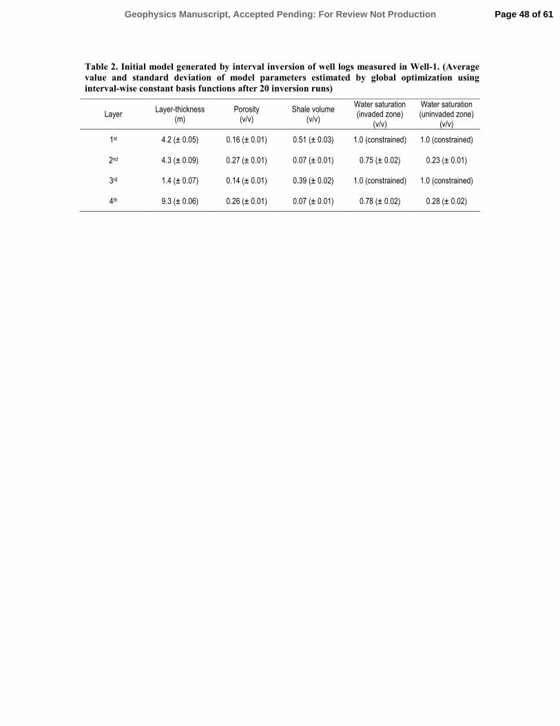
Table 2. Initial model generated by interval inversion of well logs measured in Well-1. (Average

value and standard deviation of model parameters estimated by global optimization using

interval-wise constant basis functions after 20 inversion runs)

Layer Layer-thickness

(m) Porosity

(v/v) Shale volume

(v/v)

Water saturation (invaded zone)

(v/v)

Water saturation (uninvaded zone)

(v/v)

1st 4.2 (± 0.05) 0.16 (± 0.01) 0.51 (± 0.03) 1.0 (constrained) 1.0 (constrained)

2nd 4.3 (± 0.09) 0.27 (± 0.01) 0.07 (± 0.01) 0.75 (± 0.02) 0.23 (± 0.01)

3rd 1.4 (± 0.07) 0.14 (± 0.01) 0.39 (± 0.02) 1.0 (constrained) 1.0 (constrained)

4th 9.3 (± 0.06) 0.26 (± 0.01) 0.07 (± 0.01) 0.78 (± 0.02) 0.28 (± 0.02)


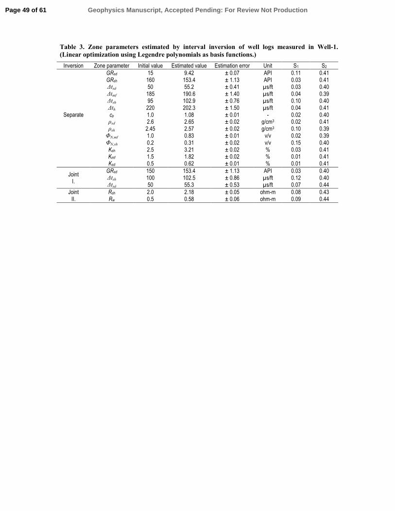
Table 3. Zone parameters estimated by interval inversion of well logs measured in Well-1.

(Linear optimization using Legendre polynomials as basis functions.)

Inversion Zone parameter Initial value Estimated value Estimation error Unit S1 S2

Separate

GRsd 15 9.42 ± 0.07 API 0.11 0.41 GRsh 160 153.4 ± 1.13 API 0.03 0.41 ∆tsd 50 55.2 ± 0.41 µs/ft 0.03 0.40 ∆tmf 185 190.6 ± 1.40 µs/ft 0.04 0.39 ∆tsh 95 102.9 ± 0.76 µs/ft 0.10 0.40 ∆th 220 202.3 ± 1.50 µs/ft 0.04 0.41 cp 1.0 1.08 ± 0.01 - 0.02 0.40 ρsd 2.6 2.65 ± 0.02 g/cm3 0.02 0.41 ρsh 2.45 2.57 ± 0.02 g/cm3 0.10 0.39

ΦN,mf 1.0 0.83 ± 0.01 v/v 0.02 0.39 ΦN,sh 0.2 0.31 ± 0.02 v/v 0.15 0.40 Ksh 2.5 3.21 ± 0.02 % 0.03 0.41 Kmf 1.5 1.82 ± 0.02 % 0.01 0.41 Ksd 0.5 0.62 ± 0.01 % 0.01 0.41

Joint I.

GRsd 150 153.4 ± 1.13 API 0.03 0.40 ∆tsh 100 102.5 ± 0.86 µs/ft 0.12 0.40 ∆tsd 50 55.3 ± 0.53 µs/ft 0.07 0.44

Joint II.

Rsh 2.0 2.18 ± 0.05 ohm-m 0.08 0.43 Rw 0.5 0.58 ± 0.06 ohm-m 0.09 0.44


Figure 1. Input well logs measured in Well-1 and uncertainty (error) ranges of log readings for local and interval inversion procedures: GR is natural gamma ray, K is potassium, ρb is bulk density, ΦN is neutron

porosity, ∆t is acoustic traveltime, Rd is resistivity, σ is standard deviation of observed data types.

1825x1009mm (96 x 96 DPI)


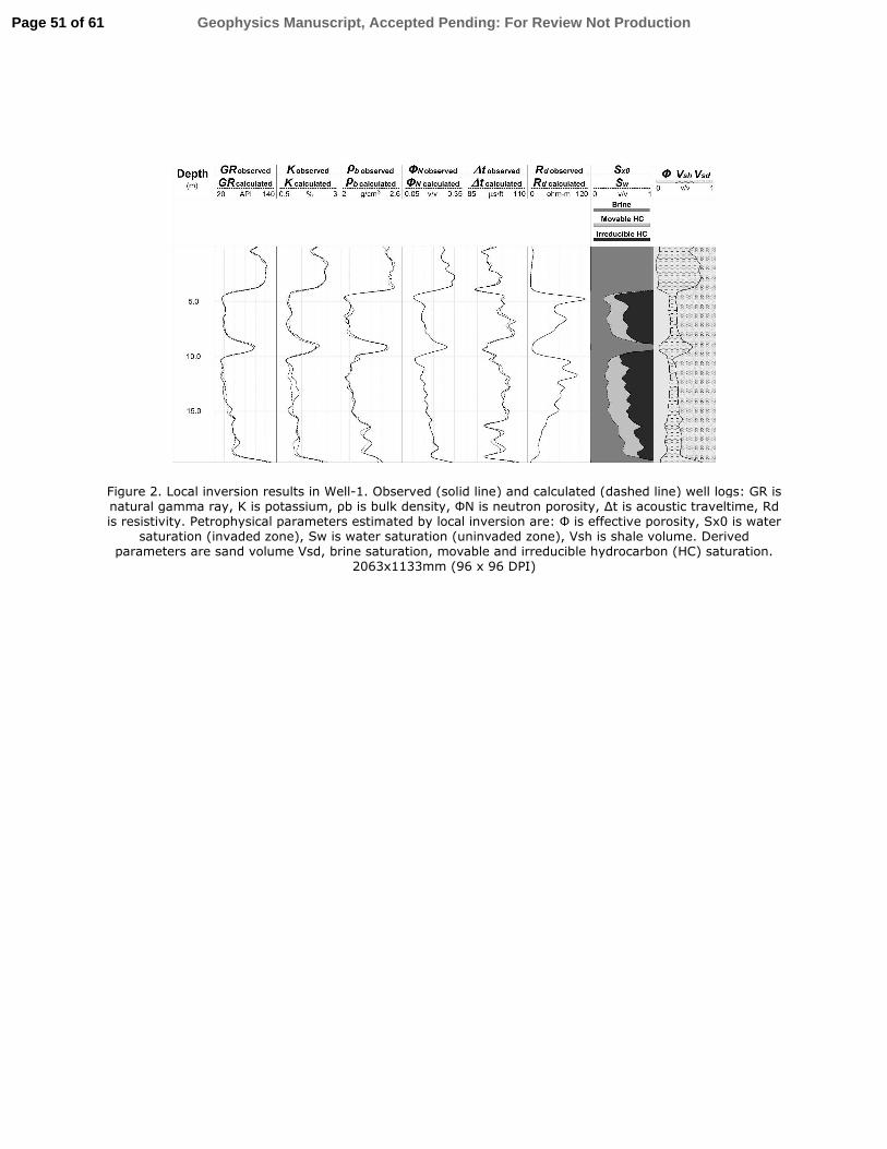
Figure 2. Local inversion results in Well-1. Observed (solid line) and calculated (dashed line) well logs: GR is natural gamma ray, K is potassium, ρb is bulk density, ΦN is neutron porosity, ∆t is acoustic traveltime, Rd is resistivity. Petrophysical parameters estimated by local inversion are: Φ is effective porosity, Sx0 is water

saturation (invaded zone), Sw is water saturation (uninvaded zone), Vsh is shale volume. Derived parameters are sand volume Vsd, brine saturation, movable and irreducible hydrocarbon (HC) saturation.

2063x1133mm (96 x 96 DPI)


Figure 3. Results of interval inversion procedure using Legendre polynomials of 44 degree as basis functions in Well-1. Estimated values of expansion coefficients for porosity (a), water saturation of uninvaded zone (b), shale content (c), water saturation of invaded zone (d) and their estimation error ranges vs. ordinal

number of expansion coefficients in the model vector. 2118x1339mm (96 x 96 DPI)


Figure 4: Correlation matrices of inversion estimates in Well-1. Absolute values of Pearson’s correlation coefficients estimated by local inversion in depth 2 m (a) and in depth 12 m (b), estimated by interval

inversion in 0−19.3 m (c). Petrophysical parameters are: Φ is effective porosity, Sx0 is water saturation

(invaded zone), Sw is water saturation (uninvaded zone), Vsh is shale volume. S is the average correlation between the model parameters; B is the vector of expansion coefficients.

1364x1197mm (120 x 120 DPI)


Figure 5: Interval inversion results in Well-1. Observed (solid line) and calculated (dashed line) well logs: GR is natural gamma ray, K is potassium, ρb is bulk density, ΦN is neutron porosity, ∆t is acoustic traveltime,

Rd is resistivity. Petrophysical parameters estimated by interval inversion are: Φ is effective porosity, Sx0 is water saturation (invaded zone), Sw is water saturation (uninvaded zone), Vsh is shale volume. Derived

parameters are Vsd is sand volume, brine saturation, movable and irreducible hydrocarbon (HC) saturation. 2063x1134mm (96 x 96 DPI)


Figure 6. Well logs of standard deviations (σ) estimated by local and interval inversion methods in Well-1. Auxiliary well logs are: GR is natural gamma ray (left panel), S is correlation average of model parameters estimated by local inversion (last but one panel on the right), D is relative data distance estimated by local

inversion (right panel). 1825x929mm (96 x 96 DPI)


Figure 7. Well logs of petrophysical parameters estimated by the local and interval inversion procedure, separately. Solid lines represent the estimated values of effective porosity Φ, water saturation for the

invaded zone Sx0 and for the uninvaded zone Sw. Dashed lines show the error bounds of petrophysical parameters calculated from the standard deviations (σ) of inversion estimates.

1587x695mm (96 x 96 DPI)


Figure 8. Well logs of correlation coefficients estimated by local and interval inversion methods in Well-1. GR as natural gamma ray (left panel) log is plotted for reference.

1825x930mm (96 x 96 DPI)


Figure 9. Porosity estimated by interval inversion procedure, deterministic modeling and core measurements in Wells 1−3. Well logs are: GR is natural gamma ray, Φ is effective porosity estimated from interval

inversion (INT-INV), CLASS interpretation system (CLASS), horizontal (H-CORE) and vertical (V-CORE) core data.

2048x1085mm (96 x 96 DPI)


Figure 10. Convergence plots of the global and linear interval inversion procedures. Trend of energy vs. number of iterations after 20 independent SA inversion runs using unit-step basis functions (a). Average

energy calculated in each iteration step (black line), average energy ± standard deviation of energies (light

and dark grey curves). Development of convergence in the subsequent DLSQ inversion procedure using Legendre polynomials as basis functions (b).

1126x1016mm (120 x 120 DPI)


Figure 11. Legendre polynomial-based interval inversion results in Well-1. Layer-thicknesses estimated by SA-based layer-by-layer interval inversion are indicated in the depth scale. Observed (solid line) and calculated (dashed line) well logs: GR is natural gamma ray, K is potassium, ρb is bulk density, ΦN is

neutron porosity, ∆t is acoustic traveltime, Rd is resistivity. Petrophysical parameters estimated by interval inversion are effective porosity Φ, water saturation (invaded zone) Sx0, water saturation (uninvaded zone) Sw, shale volume Vsh. Derived parameters are sand volume Vsd, brine saturation, movable and irreducible

hydrocarbon (HC) saturation. 2063x1129mm (96 x 96 DPI)


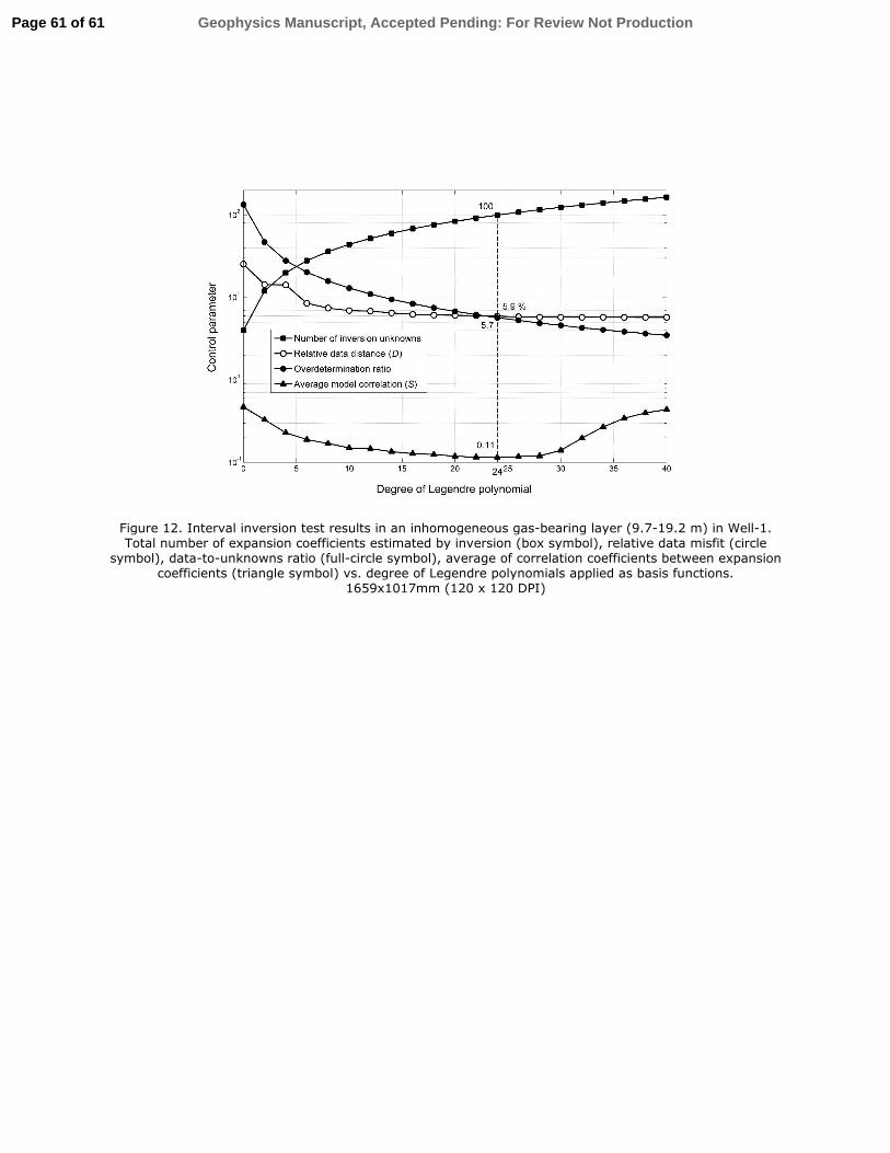
Figure 12. Interval inversion test results in an inhomogeneous gas-bearing layer (9.7-19.2 m) in Well-1. Total number of expansion coefficients estimated by inversion (box symbol), relative data misfit (circle

symbol), data-to-unknowns ratio (full-circle symbol), average of correlation coefficients between expansion coefficients (triangle symbol) vs. degree of Legendre polynomials applied as basis functions.

1659x1017mm (120 x 120 DPI)


interval inversion approach for an improved interpretation

Documents