interwar inflation, unexpected inflation, and output...
TRANSCRIPT
QEDQueen’s Economics Department Working Paper No. 1310
Interwar Inflation, Unexpected Inflation, and Output Growth
Bill DorvalQueen’s University
Gregor W. SmithQueen’s University
Department of EconomicsQueen’s University
94 University AvenueKingston, Ontario, Canada
K7L 3N6
10-2013
Interwar Inflation, Unexpected Inflation, and Output Growth
Bill Dorval and Gregor W. Smith∗
October 2014
AbstractInterwar macroeconomic history is a natural place to look for evidence on the correlationbetween output growth and inflation or unexpected inflation. We apply time-series meth-ods to measure unexpected inflation for more than twenty countries using both retail andwholesale prices. There is a significant, positive correlation between output growth andinflation for the entire period. There is little evidence that this correlation is caused byan underlying role for unexpected inflation. For wholesale price inflation in particular theoutput declines associated with deflations were larger than the output increases associatedwith inflations of the same scale.
JEL classification: E31, E37, N10
Keywords: inflation expectations, interwar period, Great Depression
∗ Department of Economics, Queen’s University, Kingston Ontario Canada K7L 3N6;[email protected]; [email protected]. We thank the Social Sciences andHumanities Research Council of Canada and the Bank of Canada fellowship programmefor support of this research. The views expressed herein are not necessarily those of theBank of Canada and are the authors’ alone. We thank conference participants at theCanadian Network for Economic History, Patrick Coe, Solomos Solomou, Kenneth West,and two referees of this journal for very constructive comments.
1. Introduction
The interwar period, with its volatility, multiple policy regimes, and international
heterogeneity, is a natural place to look for lessons on business cycles and in particular
for evidence on the relationship between monetary phenomena and the real economy.
For example, numerous countries experienced deflations during the 1920s and 1930s, and
so evidence from this period remains widely cited in more recent debates on the causes
and implications of deflation. A variety of economic theories distinguish between the
implications of the expected and unexpected components of inflation or deflation. Yet
there is little research that tries to distinguish between these two components and study
their correlations with output growth for multiple countries during the interwar period.
We use quarterly retail price indexes for 26 countries and wholesale price indexes for
24 countries in a time-series model, to try to distinguish between expected and unexpected
inflation. We find considerable variation in inflation persistence across countries. Thus the
extent to which the deflation of the early 1930s was expected to continue may well have
differed significantly across countries too.
We then see whether there is a correlation between inflation and output growth, first in
a cross-section of averages for 1930–1934 and second in the panel of countries year-by-year
for 1922–1939 with retail price inflation and for 1921–1939 with wholesale price inflation.
The cross-section provides little evidence of a significant correlation. But the panel data
allow us to control for country-specific, average growth rates over the entire interwar period.
In that statistical environment there is a clear, positive correlation between inflation and
output growth. There is little evidence that this correlation reflects an underlying one
between output growth and unexpected inflation. But there also is evidence that the
growth-inflation relationship has a kink at zero, with deflations associated with larger
output decreases than comparable inflations are with output increases.
2. Research Background
A key component in the research background is the study by Atkeson and Kehoe
(2004). They found little historical evidence of a correlation between deflations and de-
1
pressions. For the Great Depression, they measured average growth rates in real output
over 1930–1934 for 16 countries, and regressed them on a constant and average inflation
rates in this cross-section. They found a slope of 0.4 with a standard error of 0.28, thus
providing some evidence of a link, albeit with low statistical significance. Notably, they
found that the link was even weaker for other time periods. Thus they questioned the
popular view that deflations are associated with depressions.
A second key component is the study by Benhabib and Spiegel (2009). They consid-
ered the possibility that the relationship might be nonlinear: positive at low or moderate
inflation rates (or in deflations) but turning negative at high inflation rates, to form an
inverted U-shape. They studied the same set of countries as Atkeson and Kehoe, again
with averages within 5-year periods. By estimating in a panel, as opposed to a cross-
section, they allowed for country-specific fixed effects in economic growth. Measuring the
nonlinearity either with a term in squared inflation or using a threshold model, they found
a nonlinear relationship that was positive below a threshold at a moderate level of inflation
and negative or insignificant above it.
Our research also is related to studies for the US that try to measure the extent to
which the ongoing deflation during the Great Depression was anticipated. Cecchetti (1992)
argued that, once deflation began, it was largely anticipated at 3–6 month horizons. He
found evidence for anticipated deflation in (a) the US history of deflations prior to 1929, (b)
time-series models of the inflation rate, and (c) information in short-term nominal interest
rates. His time-series modelling is particularly relevant to our approach below, since we
do not have detailed information from fixed-income securities markets in the international
panel. Cecchetti measured inflation quarterly, at annual rates, and for 1919–1940 found
an AR(1) model had a coefficient of 0.52. Forecasts from this model suggested that up to
three-quarters of ongoing deflation was anticipated, so that ex ante real interest rates were
high, a likely cause of continued depression.
Nelson (1991) studied the contemporary business press and concluded that deflation
was expected after the middle of 1930. In a similar vein, Romer and Romer (2013) tracked
editorial opinion in Business Week and concluded that by the autumn of 1930 deflation
2
was anticipated and, further, that this forecast was attributed to inaction by the Fed-
eral Reserve. They too concluded that the low nominal interest rates of the period were
consistent with high, expected, real interest rates.
In contrast, Dominguez, Fair, and Shapiro (1988) summarized evidence both from
vector autoregressions and from documentary sources and concluded that the US deflation
was largely unanticipated. Hamilton (1992) observed that time-series models that have
similar in-sample fit can generate forecasts that differ widely from one another. He thus
supplemented these models with information from commodity futures markets, essentially
using the historical link between commodity prices and the overall consumer price index
as the observation equation in a Kalman filtering exercise. He concluded that expected
deflations were only about half as severe as the actual deflations that occurred in the second
and third years of the Great Depression. Evans and Wachtel (1993) described uncertainty
about Federal Reserve policy as the Depression began, and modelled inflation expectations
with a regime-switching model. They estimated investors’ views of the probability of a
return to stable prices by using information in monthly interest rates. Like Hamilton, they
concluded the deflation was largely unanticipated. This finding implies that real interest
rates were not so high once the Depression began, so that the propagation mechanism may
have been through unexpected deflation causing bankruptcy instead. Overall then, this
debate also reminds us that both anticipated and unanticipated deflation may have real
effects.
Few studies examine the degree to which interwar deflations were expected for other
countries. An exception is the study by Fregert and Jonung (2004), who looked at the
reported beliefs of employers, workers, and policymakers in Sweden, and how they differed
between the deflations of 1921–1923 and 1931–1933.
We too examine the links between inflation (or deflation) and output growth, par-
ticularly for the interwar period and for a large set of countries. We also see whether a
readily-constructed measure of unanticipated inflation affects conclusions about the cor-
relation between inflation and output growth. Our forecasting model uses the time-series
properties of inflation (as in Cecchetti, 1992) largely because the additional information
3
sources considered in the research on the US are not available for most other countries. We
have not found existing studies that use a panel of countries to assess the correlation be-
tween unexpected deflation and the business cycle in the Great Depression or the interwar
period more generally. This paper is an attempt to address this question.
3. The Information: Interwar Price and Output Data
We use both retail (or consumer) and wholesale price indexes from the League of
Nations Statistical Yearbook for 32 countries. For the US retail price level we use the CPI
from the Bureau of Labor Statistics (the original source of the League of Nations data)
because it covers a longer time span. The starting dates vary from 1920 to 1928 while
the available ending dates vary between 1938 and 1944. We end the sample at the second
quarter of 1939 so as to focus only on the interwar period. Monthly data are available
for some countries and time periods, but all results are reported for quarterly data for
comparability. Table 1 contains the list of countries, the codes used to label them, and
the country-specific time span of quarterly, retail price data. Wholesale price data are not
described in table 1 but generally begin in 1920. They are unavailable for Greece, Ireland,
and Romania but are available for an additional country: Spain.
Because the League of Nations price data begin in 1920 at the earliest, we do not
capture all of the postwar deflations or inflations. For example the UK, US, Italy, and
several other countries experienced inflation from 1919 to 1920. We also exclude episodes
of hyperinflation in the early 1920s in Austria, Germany, Hungary, and Poland. However,
there remains a great deal of heterogeneity in the inflation experiences in the panel. For
example, the data include some of the deflations associated with the restoration of the
gold standard in the early 1920s and those associated with the Great Depression, as well
as episodes of inflation later in the 1930s. Price indexes of course exist for some countries
earlier than 1920 but to our knowledge there is no international panel at high frequency
before this period.
Real output is measured in millions of 1990 international Geary-Khamis dollars per
capita. The source is Madison (2003), with significant updates by Bolt and van Zanden
4
(2013) to reflect recent research on historical national accounts. These series are at annual
frequency. Asterisks in table 1 indicate countries for which real GDP data are available
from the Maddison Project, overlapping with the League of Nations price data. This
intersection includes 26 countries for retail prices and 24 countries for wholesale prices.
An alternative to this combination of the League of Nations and Maddison data is
to use measures of real output and output deflators from Mitchell’s (2003) International
Historical Statistics. These data have three drawbacks relevant to use in our study, how-
ever. First, they are at annual frequency. That means there are not enough time-series
observations for them to be used to estimate a 4-quarter inflation forecast and measure
expected inflation. In contrast, the League of Nations data allow quarterly observations on
forecasts at this horizon. Second, the measures apply to GDP, GNP, NNP, or even switch
between these depending on the country. Third, the number of countries is 20, as opposed
to 24 or 26 with our sources, so that the Mitchell panel is smaller.
Let pit denote the price index in country i and quarter t. The inflation rate is measured
as the 4-quarter growth rate of the price index:
πit = 100 ·[(
pit
pit−4
)− 1
]. (1)
This inflation rate (as opposed to the annualized, quarter-to-quarter rate) seems appro-
priate because we later look at its correlation with the growth rate of real GDP, which is
measured at annual frequency.
For retail price inflation, table 2 contains the means, standard deviations, and standard
deviations relative to the United States, for the panel of inflation rates. Average inflation
rates varied widely across countries, with Belgium, France, Greece, Luxembourg, and
Romania all having average inflation over 4% at annual rates, while 18 of the 32 countries—
including the US and UK—on average experienced deflation. US inflation volatility (as
measured by the standard deviation) also was relatively low. Again there was considerable
variation across countries in this statistical moment.
5
4. Forecasting Model
Several sources of information available to the modern forecaster of inflation are not
present for the interwar period. National income accounts are available only at annual
frequency. We do not have access to surveys of professional forecasts (with one or two
infrequent exceptions), to inflation-indexed bond prices or, indeed, to natural covariates
such as unemployment rates or output gaps at high frequency. There is ongoing research
on the role of these covariates in forecasting inflation in contemporary data, as discussed
by Stock and Watson (2007) and Faust and Wright (2012), but we cannot check on that
role for most countries in the interwar period.
Thus we focus on univariate, time-series methods for forecasting. We estimate:
πit = μi + ρiπit−4 + ωipit−4 + εit, (2)
where t counts quarters and εit is an error term assumed to have mean zero and be
uncorrelated with the regressors. This forecasting model has the appealing features that
it involves only three parameters per country and it tends to remove any seasonality in
inflation. Most importantly, its forecasts can be averaged over quarters to produce realistic,
annual forecasts, given the 4-quarter lag, yet it still uses the high frequency of the price data
to add precision as opposed to simply estimating a time-series model in annual averages.
The parameter ρi—varying across countries—captures the persistence in actual infla-
tion and hence potentially estimates a property of expectations. The parameter ωi allows
for mean reversion (stationarity) in the price level or, equivalently, an error-correction
setup in which the inflation rate also responds to the difference between the price level
(lagged 4 quarters) and a constant. When ωi is negative a low (high) price level tends
to be followed by relatively high (low) inflation over the subsequent year. Including this
parameter thus allows for the possibility that an episode of deflation leads to expectations
of reflation. We tested the null hypothesis that there is a unit root in the price level at
the annual frequency using the test of Hylleberg, Engle, Granger, and Yoo (1990) country-
by-country and rejected it for all countries at conventional significance levels. Thus, the
quarterly data suggest that there was indeed mean reversion in interwar prices.
6
Forecasting 4 quarters ahead is challenging, and may differ from forecasting 1 quarter
ahead. But we adopt this 4-quarter horizon in the forecasting equation (2) and the def-
inition of inflation as the 4-quarter change (1) so that we can also measure the inflation
surprise at the annual horizon. The goal is then to align this with the output growth rates,
which are available only annually. It also would be interesting to study the 1-quarter-ahead
predictability of quarter-to-quarter inflation for this panel, but we do not study that issue
in this paper. Future work also might consider adding to the forecasting information set,
with indicators including the inflation rates of neighboring countries, the exchange-rate
change, or gold-standard status.
We represent the inflation forecasts in two ways, First we forecast inflation using
parameter estimates {μi, ρi, ωi} from the full interwar sample, so that forecasted inflation
is:
Et−4πit = μi + ρiπit−4 + ωipit−4. (3)
This approach has the advantage of yielding forecasts for the entire period.
Table 3 gives parameter estimates from full-sample estimation, for quarterly inflation
rates measured with both retail and wholesale price indexes, for the countries for which
Maddison (2003) and Bolt and van Zanden (2013) provided output data. Standard errors
are robust to residual autocorrelation. Notice that each value of ωi is negative and a
number of these values are statistically significant. For a number of countries a high price
level a year ago thus is associated with lower subsequent inflation, and vice versa. We also
estimated a version of the forecasting model in which the inflation rate responds to the
lagged logarithm of the price level, rather than the price level itself. The goodness-of-fit
was very similar and so the results are not shown.
Figure 1 graphs retail price inflation (the solid, black line) and expected inflation (the
dashed, gray line) for the US, using the full-sample parameter estimates from table 3 to
construct 4-quarter-ahead forecasts. For the US the estimated value of the persistence
parameter, ρi, is 0.41, so that forecasts adjust to recent inflation experience with this
weight. (They also adjust to the past price level with coefficient ωi, but that value is
very small for the US.) Figure 1 suggests that the deflation of the early 1930s was largely
7
unexpected, but that the scale of the shock declined over time (or some deflation became
expected), as expectations caught up with actual inflation to some extent. Table 3 shows
that the value of ρi is higher for several other countries, including Germany and Japan. For
those countries the fit of the forecasting model also is better and so unexpected inflation or
deflation is less variable than estimated for the US. We later test whether larger inflation
surprises are associated with larger movements in real output.
Second, we also construct recursive estimates that use only data prior to the date of
the forecast, so that forecasted inflation is:
Et−4πit = μit−4 + ρit−4πit−4 + ωit−4pit−4, (4)
where the time subscript on the parameters denotes the last observation used in estimation.
We construct the first forecast when there are 8 quarterly observations in the estimation.
But if that first forecast is not the first quarter of a calendar year, we continue to add
observations and defer forecasts until that condition is satisfied. That way, the annual
averaging always involves the same number of actual inflation rates and forecasted ones,
and the annual averages of expected and unexpected inflation always add up to actual
inflation for each year.
A benefit of adopting the recursive approach is that it uses no information from the
properties of inflation in the 1930s to estimate the parameters for constructing expected
inflation during the 1920s. But the recursive estimates of expected inflation do require a
starting date later than the first available data point, and even then the recursive estimates
early in the sample are based on relatively few observations. The delayed starting date
means that we do not measure unexpected deflations in 1921 or 1922 using these specific
measures. In any case, it might be difficult to argue they could be predicted from previous
history even were price indexes available for the prior decade and the 1914–1918 War. But
we do use the properties of such deflations to parametrize the forecasting models and hence
measure inflation expectations in the deflations of the 1930s, which are a key feature of
this historical period.
8
5. Inflation and Output Growth on Average, 1930–1934
In their study of deflations, Atkeson and Kehoe (2004) pointed out that there generally
is little evidence of a correlation between deflation and low growth in historical data.
But the one episode for which they did find a correlation was the Great Depression, and
specifically the period from 1930 to 1934 (which thus involves the levels of output and
prices from 1929 to 1934). They studied a group of 16 countries, and illustrated their
findings with a scatter plot of real output growth against inflation, with averages for each
country over those 5 years.
In this section we first duplicate their method for a larger set of 26 countries. Second,
as they noted (p 99) “we have made no attempt to distinguish anticipated from unantici-
pated deflations, while theory, of course, makes a sharp distinction.” We use the recursive
and full-sample forecasting models from section 4 to make this distinction and repeat the
scatter plot using the resulting measures of unexpected inflation or deflation. Third, we
apply the method using wholesale as well as retail prices.
To construct annual measures of inflation and unexpected inflation corresponding to
annual growth rates in real output, we average the corresponding quarterly measures within
calendar years. We then average a second time, over the years 1930–1934, just as Atkeson
and Kehoe did. Our measures of unexpected inflation rely on quarterly price indexes. We
have such measures for 12 of the 16 countries studied by Atkeson and Kehoe: Australia,
Canada, Denmark, France, Germany, Italy, Japan, the Netherlands, Norway, Sweden, the
UK, and the US. As for the remaining 4 countries in the Atkeson-Kehoe study, we do not
have data for Argentina, Brazil, or Portugal and for Spain our only data are for wholesale
prices. But we do have data for 14 additional countries, labelled with asterisks in table 1.
Figure 2 shows the scatter plot of average output growth during 1930–1934, on the
vertical axis, against average retail price inflation, on the horizontal axis, for all 26 coun-
tries. The dark circles represent actual inflation rates, while the light circles represent
unexpected inflation rates, estimated using the full sample as in equation (3). Thus the
horizontal distance between the two, for a given country, is the expected inflation rate.
9
Notice that 25 of the 26 countries experienced deflation, on average, during this 5-
year period. Greece is the one exception. But their average, annual output growth rates
varied between -5.8% for Canada and 2.0% for Finland. Overall, figure 2 provides little
evidence of a correlation between inflation and output growth or, in this case, deflation
and depression. This negative finding is influenced by countries such as Austria, which
experienced a prolonged recession with relatively modest deflation, and Japan, the UK,
and Sweden, which experienced modest growth on average with significant deflation.
We also used a regression to test for a a linear relationship between average output
growth and either inflation or unexpected inflation. Unexpected inflation was estimated
two ways, first using the full sample and then recursively. And inflation was measured
with either retail or wholesale prices. The sign of the coefficient linking the variables
was sometimes positive, but its p-value was relatively small (0.08) only in the case of the
regression for actual, wholesale inflation, in which the R2 statistic was 0.13. These findings
thus confirm the impression from figure 2.
We have added additional countries, wholesale prices, and time-series-based measures
of unexpected inflation or deflation to Atkeson and Kehoe’s study. But, if anything, these
steps weaken the evidence for a positive correlation between inflation and growth from
1930 to 1934. Studying the correlation in a cross-section of averages raises two statistical
issues, however. First, there may be information in the year-by-year observations for each
country that is obscured by the 1930–1934 averages. Second, there may be a difference in
average output growth rates across countries, unrelated to rates of inflation or deflation,
that one needs to control for in measuring the impact of inflation surprises. Atkeson and
Kehoe (2004, p 102) argued that “standard theories, either neoclassical or new Keynesian,
would have a hard time blaming Japan’s secular growth slowdown [from the 1960s to the
1990s] on its secular decline in inflation.” We concur and similarly would like to allow
for differences in average growth rates over the entire interwar period that may be due to
growth convergence or other features unrelated to inflation or deflation. The next section
studies these issues.
10
6. Inflation and Output Growth Year-by-Year, 1921/1922–1939
To further study the correlation between inflation and output growth we next examine
the interwar history year-by-year, with years indexed by the subscript τ . Data begin in
1922 for retail price inflation and in 1921 for wholesale price inflation, ending in 1939 in
each case. We relate output growth in country i and year τ , yiτ , to realized inflation
and unexpected inflation, both together and individually. To illustrate the notation, the
estimating equations thus are:
yiτ = αi + βππiτ + βu(πiτ − Eτ−1πiτ ) + εiτ . (5)
Inflation and unexpected inflation are averaged over the quarters within each calendar year
whenever at least two quarters of data are present. For 1939 we average inflation over only
the first two quarters, so as to exclude wartime data.
With a relatively short panel, working with growth rates and country-specific inter-
cepts (fixed effects) seems a reasonable specification. With the added time-series dimen-
sion, we now can identify a value αi specific to each country. The underlying economic
assumption is that a component of the long-term, average growth rate over this period was
not related to the inflation rate. Benhabib and Spiegel (2009) also controlled for country
fixed effects, in averages over successive 5-year periods.
Table 4 presents results from several special cases of equation (5) for retail price
inflation (in the upper panel) and wholesale price inflation (in the lower panel). The
number of observations reflects the fact that the starting date for the data varies by
country as shown in table 1. Estimating using forecasts with the full-sample estimates
involves the loss of one year’s data for each country, because of the lagged, dependent
variable in the forecasting model (2). Forecasting recursively involves a 2-year start-up
period that further reduces the number of observations.
For retail price inflation, the first row of table 4 contains the actual inflation rate
as the only regressor and finds it to have a coefficient of 0.29 with t-statistic of 4.8. An
inflation rate of 1% per year thus is associated with output growth of 0.29% per year. The
contrast with the lack of correlation in section 5 (figure 2) may be due to the longer time
11
span, the lack of time-averaging, or the inclusion of the country-specific fixed effects which
were not controlled for there.
The second row summarizes the regression with only unexpected inflation—measured
with full-sample forecasts—and finds that it too is significant at conventional levels of
significance. However, the third row contains results with both regressors, showing that
the coefficient on unexpected inflation is statistically insignificant when actual inflation
is included. The fourth and fifth rows then repeat this exploration but with unexpected
inflation measured with recursive forecasts. The result is the same. There is a clear
correlation between actual inflation in retail prices and growth in real output once we
control for country-specific trends.
Table 4 does not show estimates from any regressions that include expected inflation,
because the results are known automatically. Notice that equation (5) can be rearranged
as:
yiτ = αi + (βu + βπ)πiτ − βuEτ−1πiτ + εiτ . (6)
Finding that βu is insignificantly different from zero thus tells us that expected inflation
will not play a significant role when actual inflation is included in the regression. Equation
(5) also can be rearranged as:
yiτ = αi + βπEτ−1πiτ + (βu + βπ)(πiτ − Eτ−1πiτ ) + εiτ . (7)
Finding that βu is insignificantly different from zero thus also tells us that the regression
on unexpected inflation and expected inflation yields indistinguishable coefficients, so that
the combination of variables in equation (7) reproduces actual inflation. Actual inflation
thus is the clear winner in this contest to statistically explain the time-series variation in
output growth rates.
For wholesale price inflation the results (in the lower panel of table 4) are more nu-
anced. Again actual inflation clearly is correlated with output growth. But now there
is an additional, partial correlation between output growth and unexpected inflation (at
the 10% level of significance) when we forecast inflation with the full-sample parameter
estimates. Equivalently, given equation (6), expected inflation is significant at the 10%
12
level when combined with actual inflation. But with the recursive estimates there is again
no statistical role for unexpected inflation once actual inflation is included.
Notice that the expected and unexpected inflation rates are generated regressors
in that constructing them involves sampling variability in the forecasting coefficients,
{μi, ρi, ωi}. Pagan (1984) showed that the OLS standard error for unexpected inflation
is valid, when it is the only regressor, as in the second row of each panel in table 4, or
when combined with expected inflation as in equation (7). But when we use actual infla-
tion and unexpected inflation as regressors, the usual standard errors will be under-stated
in general. We therefore also constructed standard errors that correctly reflect the un-
certainty about the parameters of the forecasting model, using the method of Murphy
and Topel (1985). However, these were very similar to the unadjusted ones, and these
calculations change nothing reported in table 4. The logic is that βu is quite small. That
value scales the impact of the correction (from Murphy and Topel’s theorem 1, where the
corresponding coefficient is labelled γ) so the overall correction is small also.
Several statistical extensions to these regressions come to mind, but are not practi-
cal for the interwar period. Either adding further dynamics or studying country-specific
correlations is challenging because of the annual frequency and thus the limited number
of observations of the interwar output data. For a small number of countries with high-
frequency data one could estimate a vector autoregression and use it to measure surprises
in inflation or deflation and their impacts. Smith (2006) summarizes some existing work
in this vein for the interwar period.
7. Kinks and Curves
Table 4 shows that one can find a linear, statistical relationship between inflation and
output growth in the interwar panel, whether with retail or wholesale prices. We next
check for evidence of nonlinearities by seeing how robust the findings are to changes in the
functional form. The results are collected in table 5.
First, it is possible that the correlation between inflation and growth differed depend-
ing on whether the inflation rate was positive or negative. We use a dummy variable diτ
13
to denote observations with deflation, and by interacting this with actual inflation allow
for the correlation between inflation and output growth to differ between inflations and
deflations. The regression model then becomes:
yiτ = αi + (βπ + δdiτ )πiτ + εiτ . (8)
Thus the estimated slope is βπ for inflations and βπ + δ for deflations.
The top panel (a) of table 5 shows the results. The estimates δ (with standard errors
in brackets) are 0.14 (0.19) for retail price inflation and 0.18 (0.07) for wholesale price
inflation. In both cases, then, the coefficient linking deflation and output growth is greater
than the one linking inflation and output growth. And for wholesale price inflation this
kink at an inflation rate of zero is statistically significant at the 5% level. The output
declines associated with deflations are larger than the output increases associated with
inflations of the same scale.
Second, it also is possible that the relationship is monotonic but involves other kinks or
curves. In that case, a linear regression would be misspecified. But a simple nonparametric
method is available to check on that possibility. We rank each observation on inflation and
on output growth, then run the linear regression with the ranks instead of the original
observations. The linear functional form will be valid in ranks, even if the underlying
relationship between inflation and output growth is nonlinear, as long as that relationship
is monotone. Rank regression also may avoid some measurement errors if they are small
enough not to affect ranks. Conover (1999, section 5.6) provides an introduction and
examples of this method.
Define R[x] as the rank statistic for a variable x. Then the regression is:
R[yiτ ] = αi + λπR[πiτ ] + εiτ . (9)
The fixed effects, αi, control for country-specific average ranks of output growth rates over
the interwar period.
The middle panel (b) of table 5 contains the results. The coefficients λπ, with standard
errors in brackets, are 0.34 (0.05) for retail price inflation and 0.37 (0.05) for wholesale
14
price inflation. With just a constant term α included the coefficients become Spearman’s
rank correlation coefficients. These are 0.30 (0.05) for retail prices and 0.35 (0.05) for
wholesale prices. These positive, rank correlations are not large but they are statistically
significant at the 1% level of significance. Overall, then, there is evidence of a positive
relationship between inflation and output growth.
Third, Benhabib and Spiegel found that the correlation becomes negative at high in-
flation rates, so the relationship is not monotone, using 5-year averages for 17 countries
from 1859–2009. We follow one of their methods by including a term in squared infla-
tion, specifically to see if its coefficient is negative, capturing an inverted U-shape. The
regression is:
yiτ = αi + βππiτ + γππ2iτ + εiτ . (10)
The results are in the lower panel (c) of table 5. Squared inflation enters with a negative
coefficient—suggesting a non-monotone curve—but with a p-value of 0.92 for retail price
inflation and one of 0.13 for wholesale price inflation. Thus there is no negative associa-
tion between high inflation and growth in this panel, at conventional levels of statistical
significance.
By comparison with Benhabib and Spiegel, we study more countries but over a shorter
time span for the interwar period only, and with year-by-year data rather than 5-year av-
erages. One might suspect the annual data are simply noisier, but the goodness of fit in
our panel estimation is similar to theirs. Like these authors, we are studying correlations
rather than a causal model of output growth or inflation. But possibly even high inflation
rates (other than the central European hyperinflations of the early 1920s) were associated
with growth during the interwar period because they followed after deflations and so repre-
sented returns to more normal price levels. Figure 1 shows this pattern for inflation in the
US during 1934 when inflation was temporary, rather than heralding a shift to a perma-
nently high rate of inflation, and offset previous deflation. Our forecasting model (2) also
yielded some evidence of this mean-reverting pattern, in the form of negative coefficients
ωi.
15
8. Conclusion
This study has re-examined the relationship between inflation and growth for more
than twenty countries during the interwar period, a time of volatility in both real and nom-
inal macroeconomic variables. It also examined the further issue of whether the statistical
relationship was due to an underlying correlation with unanticipated inflation.
To model expectations we take advantage of quarterly price data to study a forecasting
model with a one-year horizon. We find considerable variation across countries in the
persistence of inflation and so possible variation across countries in inflation expectations
at the onset of the Great Depression.
We then complement the studies of Atkeson and Kehoe (2004) and Benhabib and
Spiegel (2009) by examining data from a larger set of countries and including these mea-
surements of unexpected deflation. From the cross-section of countries during 1930–1934
there is little evidence of a correlation between output growth and either inflation or un-
expected inflation. But when we use time-series variation to identify the effect (and allow
for country-specific, average, output growth rates over the entire interwar period) there
is a clear correlation between output growth and actual inflation. For the full interwar
period a 1% retail inflation rate is associated with a real growth rate of 0.18–0.39% with
95% confidence.
There are three other noteworthy findings. First, unexpected retail inflation has no
statistically significant correlation with output growth once we control for actual inflation.
There is some evidence of an additional, partial correlation between output growth and
unexpected wholesale inflation, but only for forecasts based on full-sample estimates and at
the 10% level of significance. Second, there is some evidence (again especially for wholesale
price inflation) that the relationship between output growth and inflation is nonlinear, with
a kink at zero and a steeper slope for deflations than inflations. Third, there is no significant
evidence of the slope becoming negative at high inflation rates. Bursts of inflation in the
interwar period (with the notable exception of the hyperinflations of the 1920s) often were
reflations, temporary sequels to deflations, a feature which may explain this finding.
16
References
Atkeson, Andrew and Patrick J. Kehoe (2004) Deflation and depression: Is there an em-pirical link? American Economic Review (P) 94, 99–103.
Benhabib, Jess and Mark M. Spiegel (2009) Moderate inflation and thedeflation-depression link. Journal of Money, Credit and Banking 41, 787–798.
Bolt, Jutta and Jan Leiten van Zanden (2013) The first update of the Maddison Project:Re-estimating growth before 1820. Maddison Project Working Paper 4.
Cecchetti, Stephen G. (1992) Prices during the Great Depression: Was the deflation of1930–1932 really unanticipated? American Economic Review 82, 141–156.
Conover, W. J. (1999) Practical Nonparametric Statistics. 3rd ed. New York: Wiley.
Dominguez, Kathryn M., Ray Fair, and Matthew D. Shapiro (1988) Forecasting the De-pression: Harvard versus Yale. American Economic Review 78, 595–612.
Evans, Martin, and Paul Wachtel (1993) Were price changes during the Great Depressionanticipated? Evidence from nominal interest rates. Journal of Monetary Economics32, 3–34.
Faust, Jon and Jonathan Wright (2012) Forecasting inflation. Draft for the Handbook ofForecasting, mimeo, Department of Economics, Johns Hopkins University.
Fregert, Klas and Lars Jonung (2004) Deflation dynamics in Sweden: Perceptions, expec-tations, and adjustment during the deflations of 1921–1923 and 1931–1933. chapter4 in Deflation: Current and Historical Perspectives eds R.C.K. Burdekin and P.L.Siklos. Cambridge University Press.
Hamilton, James D. (1992) Was the deflation during the Great Depression anticipated?Evidence from the commodity futures market. American Economic Review 82, 157–178.
Hylleberg, Svend, Engle, Robert F., Granger, Clive W. J. and Yoo, Byung S. (1990)Seasonal integration and cointegration. Journal of Econometrics 44, 215–238.
Maddison, Angus (2003) The World Economy: Historical Statistics. OECD DevelopmentCentre, Paris.
Mitchell, Brian R. (2003) International Historical Statistics, 1750–2000. London: Macmil-lan.
Murphy, Kevin M. and Robert H. Topel (1985) Estimation and inference in two-stepeconometric models. Journal of Business and Economic Statistics 3, 370–379.
17
Nelson, Daniel B. (1991) Was the deflation of 1929–30 anticipated? The monetary regimeas viewed by the business press. In Roger Ransom (ed.) Research in EconomicHistory 13, 1–65. Greenwich, CT: JAI Press.
Pagan, Adrian (1984) Econometric issues in the analysis of regressions with generatedregressors. International Economic Review 25, 221–247.
Romer, Christina D. and David H. Romer (2013) The missing transmission mechanism inthe monetary explanation of the Great Depression. American Economic Review (P)103, 66–72.
Smith, Gregor W. (2006) The spectre of deflation: A review of empirical evidence. Cana-dian Journal of Economics 39, 1041–1072.
Stock, James H. and Mark W. Watson (2007) Why has US inflation become harder toforecast? Journal of Money, Credit and Banking 39, 3–33.
18
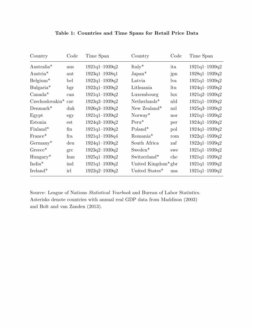
Table 1: Countries and Time Spans for Retail Price Data
Country Code Time Span Country Code Time Span
Australia* aus 1921q1–1939q2 Italy* ita 1921q1–1939q2Austria* aut 1923q1–1938q1 Japan* jpn 1928q1–1939q2Belgium* bel 1922q1–1939q2 Latvia lva 1921q1–1939q2Bulgaria* bgr 1922q1–1939q2 Lithuania ltu 1924q1–1939q2Canada* can 1921q1–1939q2 Luxembourg lux 1921q2–1939q2Czechoslovakia* cze 1923q3–1939q2 Netherlands* nld 1921q1–1939q2Denmark* dnk 1926q3–1939q2 New Zealand* nzl 1925q3–1939q2Egypt egy 1921q1–1939q2 Norway* nor 1921q1–1939q2Estonia est 1924q3–1939q2 Peru* per 1924q1–1939q2Finland* fin 1921q1–1939q2 Poland* pol 1924q1–1939q2France* fra 1921q1–1938q4 Romania* rom 1922q1–1939q2Germany* deu 1924q1–1939q2 South Africa zaf 1922q1–1939q2Greece* grc 1923q2–1939q2 Sweden* swe 1921q1–1939q2Hungary* hun 1925q1–1939q2 Switzerland* che 1921q1–1939q2India* ind 1921q1–1939q2 United Kingdom*gbr 1921q1–1939q2Ireland* irl 1922q2–1939q2 United States* usa 1921q1–1939q2
Source: League of Nations Statistical Yearbook and Bureau of Labor Statistics.Asterisks denote countries with annual real GDP data from Maddison (2003)and Bolt and van Zanden (2013).
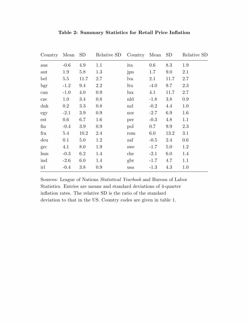
Table 2: Summary Statistics for Retail Price Inflation
Country Mean SD Relative SD Country Mean SD Relative SD
aus -0.6 4.9 1.1 ita 0.6 8.3 1.9aut 1.9 5.8 1.3 jpn 1.7 9.0 2.1bel 5.5 11.7 2.7 lva 2.1 11.7 2.7bgr -1.2 9.4 2.2 ltu -4.0 9.7 2.3can -1.0 4.0 0.9 lux 4.1 11.7 2.7cze 1.0 3.4 0.8 nld -1.8 3.8 0.9dnk 0.2 3.3 0.8 nzl -0.2 4.4 1.0egy -2.1 3.9 0.9 nor -2.7 6.9 1.6est 0.6 6.7 1.6 per -0.3 4.8 1.1fin -0.4 3.9 0.9 pol 0.7 9.9 2.3fra 5.4 10.2 2.4 rom 6.0 13.2 3.1deu 0.1 5.0 1.2 zaf -0.5 2.4 0.6grc 4.1 8.0 1.9 swe -1.7 5.0 1.2hun -0.3 6.2 1.4 che -2.1 6.0 1.4ind -2.6 6.0 1.4 gbr -1.7 4.7 1.1irl -0.4 3.8 0.9 usa -1.3 4.3 1.0
Sources: League of Nations Statistical Yearbook and Bureau of LaborStatistics. Entries are means and standard deviations of 4-quarterinflation rates. The relative SD is the ratio of the standarddeviation to that in the US. Country codes are given in table 1.
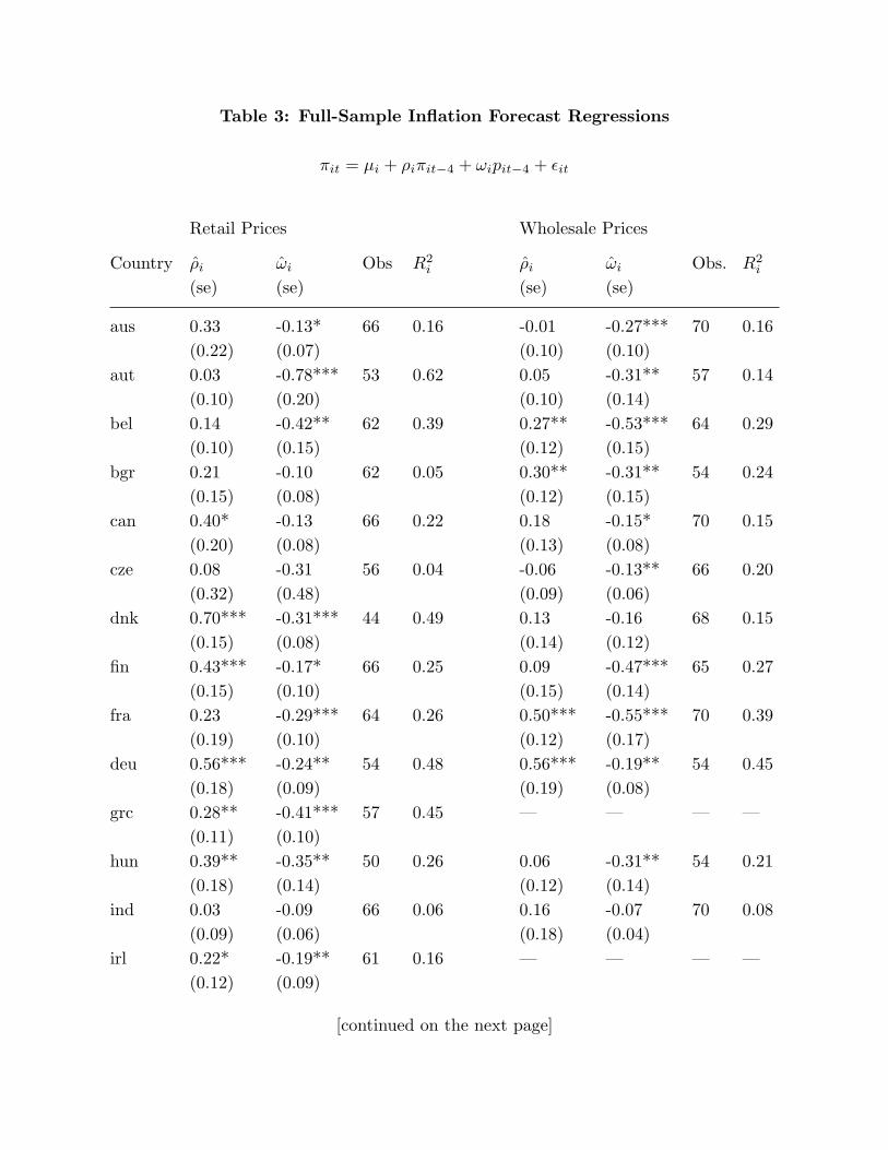
Table 3: Full-Sample Inflation Forecast Regressions
πit = μi + ρiπit−4 + ωipit−4 + εit
Retail Prices Wholesale Prices
Country ρi ωi Obs R2i ρi ωi Obs. R2
i
(se) (se) (se) (se)
aus 0.33 -0.13* 66 0.16 -0.01 -0.27*** 70 0.16(0.22) (0.07) (0.10) (0.10)
aut 0.03 -0.78*** 53 0.62 0.05 -0.31** 57 0.14(0.10) (0.20) (0.10) (0.14)
bel 0.14 -0.42** 62 0.39 0.27** -0.53*** 64 0.29(0.10) (0.15) (0.12) (0.15)
bgr 0.21 -0.10 62 0.05 0.30** -0.31** 54 0.24(0.15) (0.08) (0.12) (0.15)
can 0.40* -0.13 66 0.22 0.18 -0.15* 70 0.15(0.20) (0.08) (0.13) (0.08)
cze 0.08 -0.31 56 0.04 -0.06 -0.13** 66 0.20(0.32) (0.48) (0.09) (0.06)
dnk 0.70*** -0.31*** 44 0.49 0.13 -0.16 68 0.15(0.15) (0.08) (0.14) (0.12)
fin 0.43*** -0.17* 66 0.25 0.09 -0.47*** 65 0.27(0.15) (0.10) (0.15) (0.14)
fra 0.23 -0.29*** 64 0.26 0.50*** -0.55*** 70 0.39(0.19) (0.10) (0.12) (0.17)
deu 0.56*** -0.24** 54 0.48 0.56*** -0.19** 54 0.45(0.18) (0.09) (0.19) (0.08)
grc 0.28** -0.41*** 57 0.45 — — — —(0.11) (0.10)
hun 0.39** -0.35** 50 0.26 0.06 -0.31** 54 0.21(0.18) (0.14) (0.12) (0.14)
ind 0.03 -0.09 66 0.06 0.16 -0.07 70 0.08(0.09) (0.06) (0.18) (0.04)
irl 0.22* -0.19** 61 0.16 — — — —(0.12) (0.09)
[continued on the next page]
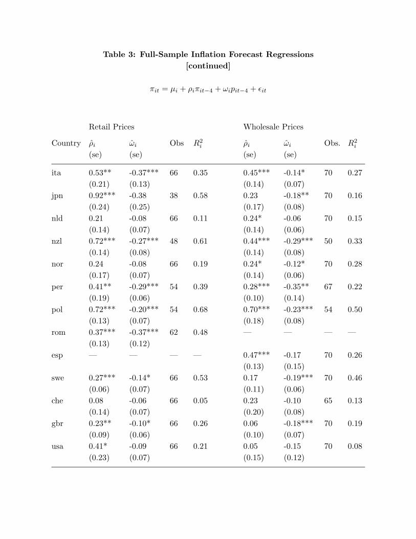
Table 3: Full-Sample Inflation Forecast Regressions[continued]
πit = μi + ρiπit−4 + ωipit−4 + εit
Retail Prices Wholesale Prices
Country ρi ωi Obs R2i ρi ωi Obs. R2
i
(se) (se) (se) (se)
ita 0.53** -0.37*** 66 0.35 0.45*** -0.14* 70 0.27(0.21) (0.13) (0.14) (0.07)
jpn 0.92*** -0.38 38 0.58 0.23 -0.18** 70 0.16(0.24) (0.25) (0.17) (0.08)
nld 0.21 -0.08 66 0.11 0.24* -0.06 70 0.15(0.14) (0.07) (0.14) (0.06)
nzl 0.72*** -0.27*** 48 0.61 0.44*** -0.29*** 50 0.33(0.14) (0.08) (0.14) (0.08)
nor 0.24 -0.08 66 0.19 0.24* -0.12* 70 0.28(0.17) (0.07) (0.14) (0.06)
per 0.41** -0.29*** 54 0.39 0.28*** -0.35** 67 0.22(0.19) (0.06) (0.10) (0.14)
pol 0.72*** -0.20*** 54 0.68 0.70*** -0.23*** 54 0.50(0.13) (0.07) (0.18) (0.08)
rom 0.37*** -0.37*** 62 0.48 — — — —(0.13) (0.12)
esp — — — — 0.47*** -0.17 70 0.26(0.13) (0.15)
swe 0.27*** -0.14* 66 0.53 0.17 -0.19*** 70 0.46(0.06) (0.07) (0.11) (0.06)
che 0.08 -0.06 66 0.05 0.23 -0.10 65 0.13(0.14) (0.07) (0.20) (0.08)
gbr 0.23** -0.10* 66 0.26 0.06 -0.18*** 70 0.19(0.09) (0.06) (0.10) (0.07)
usa 0.41* -0.09 66 0.21 0.05 -0.15 70 0.08(0.23) (0.07) (0.15) (0.12)

Notes: πit is the quarterly observation on the 4-quarter inflation rate.Country codes and quarterly time spans are given in table 1. Obsis the number of quarterly observations. Newey-West (with 4 lags)standard errors are in parentheses. p-values less than 0.01 are denoted***, less than 0.05 are denoted **, and less than 0.10 are denoted *.
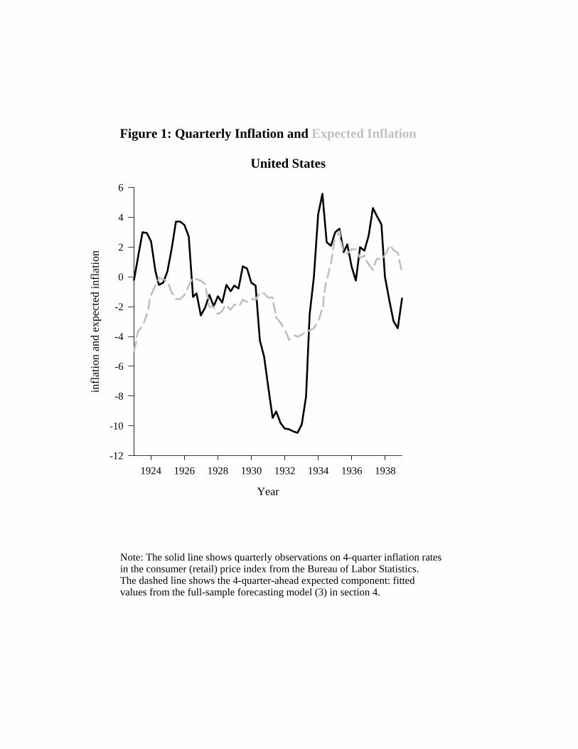
Figure 1: Quarterly Inflation and Expected Inflation
United States
Year
1924 1926 1928 1930 1932 1934 1936 1938
infla
tion
and
expe
cted
infla
tion
-12
-10
-8
-6
-4
-2
0
2
4
6
Note: The solid line shows quarterly observations on 4-quarter inflation rates in the consumer (retail) price index from the Bureau of Labor Statistics. The dashed line shows the 4-quarter-ahead expected component: fitted values from the full-sample forecasting model (3) in section 4.
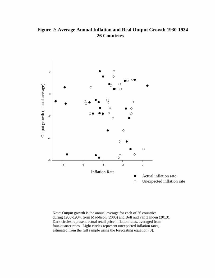
Figure 2: Average Annual Inflation and Real Output Growth 1930-1934 26 Countries
Inflation Rate
-8 -6 -4 -2 0
Out
put g
row
th (a
nnua
l ave
rage
)
-6
-4
-2
0
2
Actual inflation rateUnexpected inflation rate
Note: Output growth is the annual average for each of 26 countries during 1930-1934, from Maddison (2003) and Bolt and van Zanden (2013). Dark circles represent actual retail price inflation rates, averaged from four-quarter rates. Light circles represent unexpected inflation rates, estimated from the full sample using the forecasting equation (3).
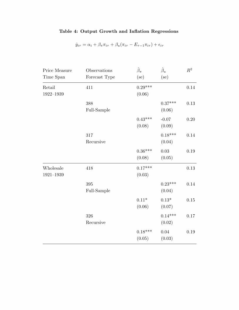
Table 4: Output Growth and Inflation Regressions
yiτ = αi + βππiτ + βu(πiτ − Eτ−1πiτ ) + εiτ
Price Measure Observations βπ βu R2
Time Span Forecast Type (se) (se)
Retail 411 0.29*** 0.141922–1939 (0.06)
388 0.37*** 0.13Full-Sample (0.06)
0.43*** -0.07 0.20(0.08) (0.09)
317 0.18*** 0.14Recursive (0.04)
0.36*** 0.03 0.19(0.08) (0.05)
Wholesale 418 0.17*** 0.131921–1939 (0.03)
395 0.23*** 0.14Full-Sample (0.04)
0.11* 0.13* 0.15(0.06) (0.07)
326 0.14*** 0.17Recursive (0.02)
0.18*** 0.04 0.19(0.05) (0.03)
Notes: yiτ is the output growth rate in country i and year τ and πiτ isthe inflation rate averaged over 4-quarter values. βπ is the coefficient oninflation; βu is the coefficient on unexpected inflation. Each system con-tains country-specific intercepts αi. There are 26 countries with retailprice data and 24 countries with wholesale price data. Recursive fore-casts use a 2-year start-up period. Brackets contains heteroskedasticity-consistent standard errors. On coefficients, p-values less than 0.01 aredenoted ***, those less than 0.05 are denoted **, and those less than0.10 are denoted *.
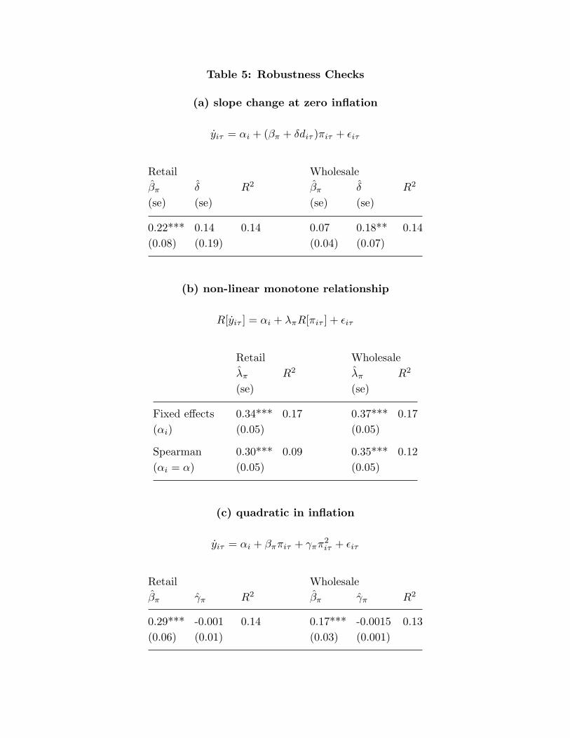
Table 5: Robustness Checks
(a) slope change at zero inflation
yiτ = αi + (βπ + δdiτ )πiτ + εiτ
Retail Wholesaleβπ δ R2 βπ δ R2
(se) (se) (se) (se)
0.22*** 0.14 0.14 0.07 0.18** 0.14(0.08) (0.19) (0.04) (0.07)
(b) non-linear monotone relationship
R[yiτ ] = αi + λπR[πiτ ] + εiτ
Retail Wholesaleλπ R2 λπ R2
(se) (se)
Fixed effects 0.34*** 0.17 0.37*** 0.17(αi) (0.05) (0.05)
Spearman 0.30*** 0.09 0.35*** 0.12(αi = α) (0.05) (0.05)
(c) quadratic in inflation
yiτ = αi + βππiτ + γππ2iτ + εiτ
Retail Wholesaleβπ γπ R2 βπ γπ R2
0.29*** -0.001 0.14 0.17*** -0.0015 0.13(0.06) (0.01) (0.03) (0.001)
Notes: yiτ is the output growth rate in country i and year τ , πiτ isthe inflation rate averaged over 4-quarter values, and αi are country-specific intercepts. There are 26 countries with retail price data (and411 observations for 1922–1939) and 24 countries with wholesale pricedata (and 418 observations for 1921–1939). In case (a) diτ = 1 fordeflations and 0 otherwise. In case (b) R[x] denotes the rank of statisticx. Brackets contains heteroskedasticity-consistent standard errors. Oncoefficients, p-values less than 0.01 are denoted ***, those less than 0.05are denoted **, and those less than 0.10 are denoted *.