introducing cos mof lo works
TRANSCRIPT

2006

Contents
IntroductionCOSMOSFloWorks Product Family . . . . . . . . . . . . . . . . . . . . . . . . . . . . . . . . . . . . . xi
Chapter 1 COSMOSFloWorks Fundamentals
How It Works . . . . . . . . . . . . . . . . . . . . . . . . . . . . . . . . . . . . . . . . . . . . . . . . . . . . . . 1-1Computational Domain . . . . . . . . . . . . . . . . . . . . . . . . . . . . . . . . . . . . . . . . . . . . 1-2Initial and Boundary Conditions . . . . . . . . . . . . . . . . . . . . . . . . . . . . . . . . . . . . . 1-2Meshing . . . . . . . . . . . . . . . . . . . . . . . . . . . . . . . . . . . . . . . . . . . . . . . . . . . . . . . . 1-3Solving. . . . . . . . . . . . . . . . . . . . . . . . . . . . . . . . . . . . . . . . . . . . . . . . . . . . . . . . . 1-3Getting Results . . . . . . . . . . . . . . . . . . . . . . . . . . . . . . . . . . . . . . . . . . . . . . . . . . 1-3
COSMOSFloWorks Project . . . . . . . . . . . . . . . . . . . . . . . . . . . . . . . . . . . . . . . . . . . 1-4Creating a Project . . . . . . . . . . . . . . . . . . . . . . . . . . . . . . . . . . . . . . . . . . . . . . . . 1-4Completing the Project Definition. . . . . . . . . . . . . . . . . . . . . . . . . . . . . . . . . . . . 1-5Deleting a Project . . . . . . . . . . . . . . . . . . . . . . . . . . . . . . . . . . . . . . . . . . . . . . . . 1-5
Goals – Basic Information . . . . . . . . . . . . . . . . . . . . . . . . . . . . . . . . . . . . . . . . . . . . 1-5Computational Domain – Basic Information . . . . . . . . . . . . . . . . . . . . . . . . . . . . . . 1-7
Symmetry Planes . . . . . . . . . . . . . . . . . . . . . . . . . . . . . . . . . . . . . . . . . . . . . . . . . 1-72D Plane Flow . . . . . . . . . . . . . . . . . . . . . . . . . . . . . . . . . . . . . . . . . . . . . . . . . . . 1-8
Initial Mesh - Basic Information. . . . . . . . . . . . . . . . . . . . . . . . . . . . . . . . . . . . . . . . 1-8Calculation Control Options - Basic Information. . . . . . . . . . . . . . . . . . . . . . . . . . . 1-9Solution-Adaptive Meshing - Basic Information . . . . . . . . . . . . . . . . . . . . . . . . . . 1-10General Options . . . . . . . . . . . . . . . . . . . . . . . . . . . . . . . . . . . . . . . . . . . . . . . . . . . 1-11Exporting Results to COSMOSWorks . . . . . . . . . . . . . . . . . . . . . . . . . . . . . . . . . . 1-14
Introducing COSMOSFloWorks i

Chapter 2 Physical Features
Analysis Type . . . . . . . . . . . . . . . . . . . . . . . . . . . . . . . . . . . . . . . . . . . . . . . . . . . . . . 2-1Heat Conduction in Solids. . . . . . . . . . . . . . . . . . . . . . . . . . . . . . . . . . . . . . . . . . . . . 2-2Time - Dependent Analysis. . . . . . . . . . . . . . . . . . . . . . . . . . . . . . . . . . . . . . . . . . . . 2-3Fluid Type and Compressibility . . . . . . . . . . . . . . . . . . . . . . . . . . . . . . . . . . . . . . . . 2-4Gravitational Effects . . . . . . . . . . . . . . . . . . . . . . . . . . . . . . . . . . . . . . . . . . . . . . . . . 2-5Turbulence. . . . . . . . . . . . . . . . . . . . . . . . . . . . . . . . . . . . . . . . . . . . . . . . . . . . . . . . . 2-5Porous Media. . . . . . . . . . . . . . . . . . . . . . . . . . . . . . . . . . . . . . . . . . . . . . . . . . . . . . . 2-6Water Vapor Condensation . . . . . . . . . . . . . . . . . . . . . . . . . . . . . . . . . . . . . . . . . . . . 2-8Non-Newtonian Liquids . . . . . . . . . . . . . . . . . . . . . . . . . . . . . . . . . . . . . . . . . . . . . . 2-8Compressible Liquids . . . . . . . . . . . . . . . . . . . . . . . . . . . . . . . . . . . . . . . . . . . . . . . . 2-9Surface-to-surface Radiation. . . . . . . . . . . . . . . . . . . . . . . . . . . . . . . . . . . . . . . . . . 2-10Compressible Flows . . . . . . . . . . . . . . . . . . . . . . . . . . . . . . . . . . . . . . . . . . . . . . . . 2-12Incompressible Flows . . . . . . . . . . . . . . . . . . . . . . . . . . . . . . . . . . . . . . . . . . . . . . . 2-13Basic Mesh . . . . . . . . . . . . . . . . . . . . . . . . . . . . . . . . . . . . . . . . . . . . . . . . . . . . . . . 2-13Travel . . . . . . . . . . . . . . . . . . . . . . . . . . . . . . . . . . . . . . . . . . . . . . . . . . . . . . . . . . . 2-13Partial Cells . . . . . . . . . . . . . . . . . . . . . . . . . . . . . . . . . . . . . . . . . . . . . . . . . . . . . . . 2-13Irregular Cells . . . . . . . . . . . . . . . . . . . . . . . . . . . . . . . . . . . . . . . . . . . . . . . . . . . . . 2-14
Chapter 3 Conditions and Tools
Overview of Conditions . . . . . . . . . . . . . . . . . . . . . . . . . . . . . . . . . . . . . . . . . . . . . . 3-1Initial Conditions – Basic Information . . . . . . . . . . . . . . . . . . . . . . . . . . . . . . . . . . . 3-4Boundary Conditions – Basic Information . . . . . . . . . . . . . . . . . . . . . . . . . . . . . . . . 3-5Transferred Boundary Conditions - Basic Information. . . . . . . . . . . . . . . . . . . . . . . 3-8Heat Sources – Basic Information. . . . . . . . . . . . . . . . . . . . . . . . . . . . . . . . . . . . . . . 3-9Fans – Basic Information . . . . . . . . . . . . . . . . . . . . . . . . . . . . . . . . . . . . . . . . . . . . 3-10Material Definition . . . . . . . . . . . . . . . . . . . . . . . . . . . . . . . . . . . . . . . . . . . . . . . . . 3-11Units – Basic Information . . . . . . . . . . . . . . . . . . . . . . . . . . . . . . . . . . . . . . . . . . . . 3-12Engineering Database – Basic Information. . . . . . . . . . . . . . . . . . . . . . . . . . . . . . . 3-12Calculator – Basic Information . . . . . . . . . . . . . . . . . . . . . . . . . . . . . . . . . . . . . . . . 3-13
ii Introducing COSMOSFloWorks

Chapter 4 Wizard
Wizard and Navigator . . . . . . . . . . . . . . . . . . . . . . . . . . . . . . . . . . . . . . . . . . . . . . . .4-1Project Configuration . . . . . . . . . . . . . . . . . . . . . . . . . . . . . . . . . . . . . . . . . . . . . . . . .4-2Unit System . . . . . . . . . . . . . . . . . . . . . . . . . . . . . . . . . . . . . . . . . . . . . . . . . . . . . . . .4-2Analysis Type. . . . . . . . . . . . . . . . . . . . . . . . . . . . . . . . . . . . . . . . . . . . . . . . . . . . . . .4-3Default Fluid . . . . . . . . . . . . . . . . . . . . . . . . . . . . . . . . . . . . . . . . . . . . . . . . . . . . . . .4-6Default Solid . . . . . . . . . . . . . . . . . . . . . . . . . . . . . . . . . . . . . . . . . . . . . . . . . . . . . . .4-7Default Wall Conditions . . . . . . . . . . . . . . . . . . . . . . . . . . . . . . . . . . . . . . . . . . . . . .4-8Initial and Ambient Conditions . . . . . . . . . . . . . . . . . . . . . . . . . . . . . . . . . . . . . . . .4-10Results and Geometry Resolution . . . . . . . . . . . . . . . . . . . . . . . . . . . . . . . . . . . . . .4-13Rotation . . . . . . . . . . . . . . . . . . . . . . . . . . . . . . . . . . . . . . . . . . . . . . . . . . . . . . . . . .4-15Rotation Axis . . . . . . . . . . . . . . . . . . . . . . . . . . . . . . . . . . . . . . . . . . . . . . . . . . . . . .4-16Select Results to Transfer. . . . . . . . . . . . . . . . . . . . . . . . . . . . . . . . . . . . . . . . . . . . .4-17
Chapter 5 Working with Project
New Project . . . . . . . . . . . . . . . . . . . . . . . . . . . . . . . . . . . . . . . . . . . . . . . . . . . . . . . .5-1Clone Project . . . . . . . . . . . . . . . . . . . . . . . . . . . . . . . . . . . . . . . . . . . . . . . . . . . . . . .5-2Template. . . . . . . . . . . . . . . . . . . . . . . . . . . . . . . . . . . . . . . . . . . . . . . . . . . . . . . . . . .5-3COSMOSFloWorks Default Template . . . . . . . . . . . . . . . . . . . . . . . . . . . . . . . . . . .5-4Clear Configuration . . . . . . . . . . . . . . . . . . . . . . . . . . . . . . . . . . . . . . . . . . . . . . . . . .5-5Edit Comment . . . . . . . . . . . . . . . . . . . . . . . . . . . . . . . . . . . . . . . . . . . . . . . . . . . . . .5-5Summary . . . . . . . . . . . . . . . . . . . . . . . . . . . . . . . . . . . . . . . . . . . . . . . . . . . . . . . . . .5-5Rebuild Project. . . . . . . . . . . . . . . . . . . . . . . . . . . . . . . . . . . . . . . . . . . . . . . . . . . . . .5-6Copy Features among Projects. . . . . . . . . . . . . . . . . . . . . . . . . . . . . . . . . . . . . . . . . .5-6Parameter Editor. . . . . . . . . . . . . . . . . . . . . . . . . . . . . . . . . . . . . . . . . . . . . . . . . . . . .5-6Component Control . . . . . . . . . . . . . . . . . . . . . . . . . . . . . . . . . . . . . . . . . . . . . . . . . .5-7Specifying Components Transparent for the Heat Radiation. . . . . . . . . . . . . . . . . . .5-8Excluding Unused Components from the Analysis . . . . . . . . . . . . . . . . . . . . . . . . . .5-9
Working with Lightweight Parts. . . . . . . . . . . . . . . . . . . . . . . . . . . . . . . . . . . . .5-10
Introducing COSMOSFloWorks iii
Chapter 6 General Settings
General Settings – Overview. . . . . . . . . . . . . . . . . . . . . . . . . . . . . . . . . . . . . . . . . . . 6-1Analysis Type . . . . . . . . . . . . . . . . . . . . . . . . . . . . . . . . . . . . . . . . . . . . . . . . . . . . . . 6-2Fluids. . . . . . . . . . . . . . . . . . . . . . . . . . . . . . . . . . . . . . . . . . . . . . . . . . . . . . . . . . . . . 6-4Solids. . . . . . . . . . . . . . . . . . . . . . . . . . . . . . . . . . . . . . . . . . . . . . . . . . . . . . . . . . . . . 6-6Default Wall Conditions . . . . . . . . . . . . . . . . . . . . . . . . . . . . . . . . . . . . . . . . . . . . . . 6-7Initial and Ambient Conditions . . . . . . . . . . . . . . . . . . . . . . . . . . . . . . . . . . . . . . . . 6-10Rotation . . . . . . . . . . . . . . . . . . . . . . . . . . . . . . . . . . . . . . . . . . . . . . . . . . . . . . . . . . 6-12
Chapter 7 Computational Domain
Computational Domain . . . . . . . . . . . . . . . . . . . . . . . . . . . . . . . . . . . . . . . . . . . . . . . 7-1Symmetry Planes. . . . . . . . . . . . . . . . . . . . . . . . . . . . . . . . . . . . . . . . . . . . . . . . . . . . 7-2
Chapter 8 Fluid Subdomains
Creating a Fluid Subdomain . . . . . . . . . . . . . . . . . . . . . . . . . . . . . . . . . . . . . . . . . . . 8-1Specifying Fluids for Fluid Subdomain . . . . . . . . . . . . . . . . . . . . . . . . . . . . . . . . . . 8-2Specifying Initial Conditions for Fluid Subdomain . . . . . . . . . . . . . . . . . . . . . . . . . 8-2
Chapter 9 Rotating Regions
Creating a Rotating Region . . . . . . . . . . . . . . . . . . . . . . . . . . . . . . . . . . . . . . . . . . . . 9-1
Chapter 10 Solid Materials
Creating a Solid Material . . . . . . . . . . . . . . . . . . . . . . . . . . . . . . . . . . . . . . . . . . . . 10-1Insert Material from Model . . . . . . . . . . . . . . . . . . . . . . . . . . . . . . . . . . . . . . . . . . . 10-2
Chapter 11 Boundary Conditions
Creating a Boundary Condition. . . . . . . . . . . . . . . . . . . . . . . . . . . . . . . . . . . . . . . . 11-1Specifying Boundary Condition Parameters . . . . . . . . . . . . . . . . . . . . . . . . . . . . . . 11-3Specifying Moving Wall . . . . . . . . . . . . . . . . . . . . . . . . . . . . . . . . . . . . . . . . . . . . . 11-7Boundary Conditions in Gas Analyses . . . . . . . . . . . . . . . . . . . . . . . . . . . . . . . . . . 11-9
Inlet Conditions . . . . . . . . . . . . . . . . . . . . . . . . . . . . . . . . . . . . . . . . . . . . . . . . . 11-9Outlet Conditions . . . . . . . . . . . . . . . . . . . . . . . . . . . . . . . . . . . . . . . . . . . . . . . 11-10
iv Introducing COSMOSFloWorks

Chapter 12 Transferred Boundary Conditions
Creating Transferred Boundary Conditions . . . . . . . . . . . . . . . . . . . . . . . . . . . . . . .12-1Selecting Results to Transfer . . . . . . . . . . . . . . . . . . . . . . . . . . . . . . . . . . . . . . . . . .12-2Browse for Project . . . . . . . . . . . . . . . . . . . . . . . . . . . . . . . . . . . . . . . . . . . . . . . . . .12-2Specifying Type of Conditions . . . . . . . . . . . . . . . . . . . . . . . . . . . . . . . . . . . . . . . .12-2
Chapter 13 Fans
Creating a Fan . . . . . . . . . . . . . . . . . . . . . . . . . . . . . . . . . . . . . . . . . . . . . . . . . . . . .13-1Specifying Fan Parameters. . . . . . . . . . . . . . . . . . . . . . . . . . . . . . . . . . . . . . . . . . . .13-3
Chapter 14 Heat Sources
Creating a Surface Source . . . . . . . . . . . . . . . . . . . . . . . . . . . . . . . . . . . . . . . . . . . .14-1Creating a Volume Source . . . . . . . . . . . . . . . . . . . . . . . . . . . . . . . . . . . . . . . . . . . .14-2
Chapter 15 Radiative Surfaces
Creating a Radiative Surface . . . . . . . . . . . . . . . . . . . . . . . . . . . . . . . . . . . . . . . . . .15-1
Chapter 16 Contact Resistances
Creating a Contact Resistance . . . . . . . . . . . . . . . . . . . . . . . . . . . . . . . . . . . . . . . . .16-1
Chapter 17 Heat Sink Simulations
Creating a Heat Sink Simulation . . . . . . . . . . . . . . . . . . . . . . . . . . . . . . . . . . . . . . .17-1
Chapter 18 Porous Media
Creating a Porous Medium. . . . . . . . . . . . . . . . . . . . . . . . . . . . . . . . . . . . . . . . . . . .18-1Specifying Porous Medium Parameters . . . . . . . . . . . . . . . . . . . . . . . . . . . . . . . . . .18-2
Chapter 19 Initial Conditions
Creating an Initial Condition . . . . . . . . . . . . . . . . . . . . . . . . . . . . . . . . . . . . . . . . . .19-1Specifying Initial Condition Parameters . . . . . . . . . . . . . . . . . . . . . . . . . . . . . . . . .19-2
Chapter 20 Goals
Global Goal . . . . . . . . . . . . . . . . . . . . . . . . . . . . . . . . . . . . . . . . . . . . . . . . . . . . . . .20-1
Introducing COSMOSFloWorks v
Surface Goal . . . . . . . . . . . . . . . . . . . . . . . . . . . . . . . . . . . . . . . . . . . . . . . . . . . . . . 20-2Volume Goal . . . . . . . . . . . . . . . . . . . . . . . . . . . . . . . . . . . . . . . . . . . . . . . . . . . . . . 20-4Equation Goal . . . . . . . . . . . . . . . . . . . . . . . . . . . . . . . . . . . . . . . . . . . . . . . . . . . . . 20-6
Chapter 21 Meshing
Automatic Settings for Initial Mesh . . . . . . . . . . . . . . . . . . . . . . . . . . . . . . . . . . . . 21-1Extract Mesh from the Results File. . . . . . . . . . . . . . . . . . . . . . . . . . . . . . . . . . . . . 21-2Creating an Initial Mesh . . . . . . . . . . . . . . . . . . . . . . . . . . . . . . . . . . . . . . . . . . . . . 21-3Resolving the Interface Between Substances . . . . . . . . . . . . . . . . . . . . . . . . . . . . . 21-5Refining Cells by Type . . . . . . . . . . . . . . . . . . . . . . . . . . . . . . . . . . . . . . . . . . . . . . 21-8Narrow Channel Resolution . . . . . . . . . . . . . . . . . . . . . . . . . . . . . . . . . . . . . . . . . . 21-9Specifying Control Planes. . . . . . . . . . . . . . . . . . . . . . . . . . . . . . . . . . . . . . . . . . . 21-10Control Plane Position. . . . . . . . . . . . . . . . . . . . . . . . . . . . . . . . . . . . . . . . . . . . . . 21-11Specifying Local Initial Mesh . . . . . . . . . . . . . . . . . . . . . . . . . . . . . . . . . . . . . . . . 21-12Specifying Automatic Settings for Local Initial Mesh . . . . . . . . . . . . . . . . . . . . . 21-13Resolving the Interface within Local Regions . . . . . . . . . . . . . . . . . . . . . . . . . . . 21-14Refining Cells within Local Regions . . . . . . . . . . . . . . . . . . . . . . . . . . . . . . . . . . 21-15Narrow Channels Resolution in Local Regions . . . . . . . . . . . . . . . . . . . . . . . . . . 21-15
Chapter 22 Tools
Dependency. . . . . . . . . . . . . . . . . . . . . . . . . . . . . . . . . . . . . . . . . . . . . . . . . . . . . . . 22-1Unit System. . . . . . . . . . . . . . . . . . . . . . . . . . . . . . . . . . . . . . . . . . . . . . . . . . . . . . . 22-2Creating a Custom Unit. . . . . . . . . . . . . . . . . . . . . . . . . . . . . . . . . . . . . . . . . . . . . . 22-3Engineering Database . . . . . . . . . . . . . . . . . . . . . . . . . . . . . . . . . . . . . . . . . . . . . . . 22-3
Specifying Custom Visualization Parameters . . . . . . . . . . . . . . . . . . . . . . . . . . 22-5Calculator . . . . . . . . . . . . . . . . . . . . . . . . . . . . . . . . . . . . . . . . . . . . . . . . . . . . . . . . 22-6
Import a Value from the Engineering Database . . . . . . . . . . . . . . . . . . . . . . . . 22-7Tank Evacuation . . . . . . . . . . . . . . . . . . . . . . . . . . . . . . . . . . . . . . . . . . . . . . . . 22-7Technical Background . . . . . . . . . . . . . . . . . . . . . . . . . . . . . . . . . . . . . . . . . . . . 22-9
Parametric Study . . . . . . . . . . . . . . . . . . . . . . . . . . . . . . . . . . . . . . . . . . . . . . . . . . 22-11Making a Parametric Study . . . . . . . . . . . . . . . . . . . . . . . . . . . . . . . . . . . . . . . 22-11Parametric Study - Specifying a Variable Parameter . . . . . . . . . . . . . . . . . . . 22-12Parametric Study - Selecting a Goal . . . . . . . . . . . . . . . . . . . . . . . . . . . . . . . . 22-13
vi Introducing COSMOSFloWorks

Parametric Study - Parameter Definition . . . . . . . . . . . . . . . . . . . . . . . . . . . . .22-13Parametric Study - Finishing Conditions . . . . . . . . . . . . . . . . . . . . . . . . . . . . .22-14Parametric Study - Calculation . . . . . . . . . . . . . . . . . . . . . . . . . . . . . . . . . . . . .22-14
Simplifying the Model . . . . . . . . . . . . . . . . . . . . . . . . . . . . . . . . . . . . . . . . . . . . . .22-15Check Geometry. . . . . . . . . . . . . . . . . . . . . . . . . . . . . . . . . . . . . . . . . . . . . . . . . . .22-16Selection Filter . . . . . . . . . . . . . . . . . . . . . . . . . . . . . . . . . . . . . . . . . . . . . . . . . . . .22-17COSMOSFloWorks Toolbars . . . . . . . . . . . . . . . . . . . . . . . . . . . . . . . . . . . . . . . .22-19
Chapter 23 Calculation Control Options
Calculation Control Options - Overview . . . . . . . . . . . . . . . . . . . . . . . . . . . . . . . . .23-1Finishing the Calculation . . . . . . . . . . . . . . . . . . . . . . . . . . . . . . . . . . . . . . . . . . . . .23-2Refining Mesh During Calculation . . . . . . . . . . . . . . . . . . . . . . . . . . . . . . . . . . . . .23-3Table of Refinements . . . . . . . . . . . . . . . . . . . . . . . . . . . . . . . . . . . . . . . . . . . . . . . .23-6Saving Results . . . . . . . . . . . . . . . . . . . . . . . . . . . . . . . . . . . . . . . . . . . . . . . . . . . . .23-6Advanced Settings . . . . . . . . . . . . . . . . . . . . . . . . . . . . . . . . . . . . . . . . . . . . . . . . . .23-7
Flow Freezing . . . . . . . . . . . . . . . . . . . . . . . . . . . . . . . . . . . . . . . . . . . . . . . . . . .23-7Manual Time Step. . . . . . . . . . . . . . . . . . . . . . . . . . . . . . . . . . . . . . . . . . . . . . . .23-7Radiation View Factor . . . . . . . . . . . . . . . . . . . . . . . . . . . . . . . . . . . . . . . . . . . .23-8
Table of Savings. . . . . . . . . . . . . . . . . . . . . . . . . . . . . . . . . . . . . . . . . . . . . . . . . . . .23-8Automatic Settings by Reset . . . . . . . . . . . . . . . . . . . . . . . . . . . . . . . . . . . . . . . . . .23-8
Chapter 24 Solving
Running the Calculation. . . . . . . . . . . . . . . . . . . . . . . . . . . . . . . . . . . . . . . . . . . . . .24-1Batch Run. . . . . . . . . . . . . . . . . . . . . . . . . . . . . . . . . . . . . . . . . . . . . . . . . . . . . . . . .24-3Specifying Computers for Network Solving . . . . . . . . . . . . . . . . . . . . . . . . . . . . . .24-4
Chapter 25 Monitoring Calculation
Monitoring Calculation - Overview . . . . . . . . . . . . . . . . . . . . . . . . . . . . . . . . . . . . .25-1Information and Warnings . . . . . . . . . . . . . . . . . . . . . . . . . . . . . . . . . . . . . . . . . . . .25-3Goal Table . . . . . . . . . . . . . . . . . . . . . . . . . . . . . . . . . . . . . . . . . . . . . . . . . . . . . . . .25-6Creating and Editing Goal Plot . . . . . . . . . . . . . . . . . . . . . . . . . . . . . . . . . . . . . . . .25-7Goal Plot. . . . . . . . . . . . . . . . . . . . . . . . . . . . . . . . . . . . . . . . . . . . . . . . . . . . . . . . . .25-8Goal Plot Settings. . . . . . . . . . . . . . . . . . . . . . . . . . . . . . . . . . . . . . . . . . . . . . . . . . .25-8
Introducing COSMOSFloWorks vii

Goal Values . . . . . . . . . . . . . . . . . . . . . . . . . . . . . . . . . . . . . . . . . . . . . . . . . . . . . . 25-10Preview Results . . . . . . . . . . . . . . . . . . . . . . . . . . . . . . . . . . . . . . . . . . . . . . . . . . . 25-10Creating and Editing Preview . . . . . . . . . . . . . . . . . . . . . . . . . . . . . . . . . . . . . . . . 25-11Preview Settings . . . . . . . . . . . . . . . . . . . . . . . . . . . . . . . . . . . . . . . . . . . . . . . . . . 25-13Preview Image Attributes . . . . . . . . . . . . . . . . . . . . . . . . . . . . . . . . . . . . . . . . . . . 25-14Preview Options . . . . . . . . . . . . . . . . . . . . . . . . . . . . . . . . . . . . . . . . . . . . . . . . . . 25-14Preview Region . . . . . . . . . . . . . . . . . . . . . . . . . . . . . . . . . . . . . . . . . . . . . . . . . . . 25-15Min/Max Table . . . . . . . . . . . . . . . . . . . . . . . . . . . . . . . . . . . . . . . . . . . . . . . . . . . 25-15Refinement . . . . . . . . . . . . . . . . . . . . . . . . . . . . . . . . . . . . . . . . . . . . . . . . . . . . . . 25-15Refinement Table . . . . . . . . . . . . . . . . . . . . . . . . . . . . . . . . . . . . . . . . . . . . . . . . . 25-16Suspend Options . . . . . . . . . . . . . . . . . . . . . . . . . . . . . . . . . . . . . . . . . . . . . . . . . . 25-16Monitor Toolbar . . . . . . . . . . . . . . . . . . . . . . . . . . . . . . . . . . . . . . . . . . . . . . . . . . 25-17
Chapter 26 Getting Results
Getting Results . . . . . . . . . . . . . . . . . . . . . . . . . . . . . . . . . . . . . . . . . . . . . . . . . . . . 26-1Loading Results. . . . . . . . . . . . . . . . . . . . . . . . . . . . . . . . . . . . . . . . . . . . . . . . . . . . 26-3Surface Related Parameters. . . . . . . . . . . . . . . . . . . . . . . . . . . . . . . . . . . . . . . . . . . 26-4Display Mode . . . . . . . . . . . . . . . . . . . . . . . . . . . . . . . . . . . . . . . . . . . . . . . . . . . . . 26-5Results Summary. . . . . . . . . . . . . . . . . . . . . . . . . . . . . . . . . . . . . . . . . . . . . . . . . . . 26-7Automatic Results Processing for Set of Calculations . . . . . . . . . . . . . . . . . . . . . . 26-7View Settings . . . . . . . . . . . . . . . . . . . . . . . . . . . . . . . . . . . . . . . . . . . . . . . . . . . . . 26-8
Contours . . . . . . . . . . . . . . . . . . . . . . . . . . . . . . . . . . . . . . . . . . . . . . . . . . . . . . . 26-9Isolines . . . . . . . . . . . . . . . . . . . . . . . . . . . . . . . . . . . . . . . . . . . . . . . . . . . . . . . 26-10Vectors . . . . . . . . . . . . . . . . . . . . . . . . . . . . . . . . . . . . . . . . . . . . . . . . . . . . . . . 26-11Flow Trajectories . . . . . . . . . . . . . . . . . . . . . . . . . . . . . . . . . . . . . . . . . . . . . . . 26-12Isosurfaces . . . . . . . . . . . . . . . . . . . . . . . . . . . . . . . . . . . . . . . . . . . . . . . . . . . . 26-123D Profile Plot . . . . . . . . . . . . . . . . . . . . . . . . . . . . . . . . . . . . . . . . . . . . . . . . . 26-14Options. . . . . . . . . . . . . . . . . . . . . . . . . . . . . . . . . . . . . . . . . . . . . . . . . . . . . . . 26-14Coordinate System. . . . . . . . . . . . . . . . . . . . . . . . . . . . . . . . . . . . . . . . . . . . . . 26-16
Plot Manager . . . . . . . . . . . . . . . . . . . . . . . . . . . . . . . . . . . . . . . . . . . . . . . . . . . . . 26-17Parameter List . . . . . . . . . . . . . . . . . . . . . . . . . . . . . . . . . . . . . . . . . . . . . . . . . . . . 26-17Displaying Refinement Information . . . . . . . . . . . . . . . . . . . . . . . . . . . . . . . . . . . 26-17Min/Max Table . . . . . . . . . . . . . . . . . . . . . . . . . . . . . . . . . . . . . . . . . . . . . . . . . . . 26-18
viii Introducing COSMOSFloWorks

Mesh Visualization. . . . . . . . . . . . . . . . . . . . . . . . . . . . . . . . . . . . . . . . . . . . . . . . .26-18Excel Output of Parameters in Cells . . . . . . . . . . . . . . . . . . . . . . . . . . . . . . . . . . .26-19ASCII Output of Parameters in Cells. . . . . . . . . . . . . . . . . . . . . . . . . . . . . . . . . . .26-19Creating a Cut Plot . . . . . . . . . . . . . . . . . . . . . . . . . . . . . . . . . . . . . . . . . . . . . . . . .26-20
Cut Plot Settings . . . . . . . . . . . . . . . . . . . . . . . . . . . . . . . . . . . . . . . . . . . . . . . 26-22Cut Plot Region. . . . . . . . . . . . . . . . . . . . . . . . . . . . . . . . . . . . . . . . . . . . . . . . 26-23Animation of Cut Plots . . . . . . . . . . . . . . . . . . . . . . . . . . . . . . . . . . . . . . . . . . 26-24
Creating a 3D Profile Plot . . . . . . . . . . . . . . . . . . . . . . . . . . . . . . . . . . . . . . . . . . .26-243D Profile Plot Region . . . . . . . . . . . . . . . . . . . . . . . . . . . . . . . . . . . . . . . . . . 26-26Animation of 3D Profile Plots . . . . . . . . . . . . . . . . . . . . . . . . . . . . . . . . . . . . 26-27
Creating a Surface Plot. . . . . . . . . . . . . . . . . . . . . . . . . . . . . . . . . . . . . . . . . . . . . .26-27Surface Plot Settings . . . . . . . . . . . . . . . . . . . . . . . . . . . . . . . . . . . . . . . . . . . . 26-28Surface Plot Region . . . . . . . . . . . . . . . . . . . . . . . . . . . . . . . . . . . . . . . . . . . . 26-29
Creating Isosurfaces . . . . . . . . . . . . . . . . . . . . . . . . . . . . . . . . . . . . . . . . . . . . . . . .26-29Displaying Flow Trajectories . . . . . . . . . . . . . . . . . . . . . . . . . . . . . . . . . . . . . . . . .26-30
Flow Trajectories Settings . . . . . . . . . . . . . . . . . . . . . . . . . . . . . . . . . . . . . . . 26-31Export Trajectories Data . . . . . . . . . . . . . . . . . . . . . . . . . . . . . . . . . . . . . . . . . 26-32Flow Trajectories Table . . . . . . . . . . . . . . . . . . . . . . . . . . . . . . . . . . . . . . . . . 26-33Animation of Flow Trajectories . . . . . . . . . . . . . . . . . . . . . . . . . . . . . . . . . . . 26-33
Particle Study . . . . . . . . . . . . . . . . . . . . . . . . . . . . . . . . . . . . . . . . . . . . . . . . . . . . .26-34Injection . . . . . . . . . . . . . . . . . . . . . . . . . . . . . . . . . . . . . . . . . . . . . . . . . . . . . 26-35Wall Boundary Condition . . . . . . . . . . . . . . . . . . . . . . . . . . . . . . . . . . . . . . . . 26-37Computational Domain. . . . . . . . . . . . . . . . . . . . . . . . . . . . . . . . . . . . . . . . . . 26-37Settings . . . . . . . . . . . . . . . . . . . . . . . . . . . . . . . . . . . . . . . . . . . . . . . . . . . . . . 26-38Save Options . . . . . . . . . . . . . . . . . . . . . . . . . . . . . . . . . . . . . . . . . . . . . . . . . . 26-38Physical Models . . . . . . . . . . . . . . . . . . . . . . . . . . . . . . . . . . . . . . . . . . . . . . . 26-39File Format for Injection Definition . . . . . . . . . . . . . . . . . . . . . . . . . . . . . . . . 26-40Particle Study - Results. . . . . . . . . . . . . . . . . . . . . . . . . . . . . . . . . . . . . . . . . . 26-41Exporting into Excel . . . . . . . . . . . . . . . . . . . . . . . . . . . . . . . . . . . . . . . . . . . . 26-42Particles Tracing Summary. . . . . . . . . . . . . . . . . . . . . . . . . . . . . . . . . . . . . . . 26-42Particles Trajectories Display Options . . . . . . . . . . . . . . . . . . . . . . . . . . . . . . 26-43Animation of Particles Trajectories . . . . . . . . . . . . . . . . . . . . . . . . . . . . . . . . 26-43
Creating an XY-Plot. . . . . . . . . . . . . . . . . . . . . . . . . . . . . . . . . . . . . . . . . . . . . . . .26-43Displaying Surface Parameters . . . . . . . . . . . . . . . . . . . . . . . . . . . . . . . . . . . . . . .26-46
Scenario for Surface Parameters. . . . . . . . . . . . . . . . . . . . . . . . . . . . . . . . . . . 26-47Displaying Volume Parameters . . . . . . . . . . . . . . . . . . . . . . . . . . . . . . . . . . . . . . .26-48
Scenario for Volume Parameters . . . . . . . . . . . . . . . . . . . . . . . . . . . . . . . . . . 26-49
Introducing COSMOSFloWorks ix

Displaying Point Parameters . . . . . . . . . . . . . . . . . . . . . . . . . . . . . . . . . . . . . . . . . 26-49Point Parameters Table . . . . . . . . . . . . . . . . . . . . . . . . . . . . . . . . . . . . . . . . . . 26-51Scenario for Point Parameters . . . . . . . . . . . . . . . . . . . . . . . . . . . . . . . . . . . . . 26-52
Creating a Goal Plot . . . . . . . . . . . . . . . . . . . . . . . . . . . . . . . . . . . . . . . . . . . . . . . 26-52Save Image . . . . . . . . . . . . . . . . . . . . . . . . . . . . . . . . . . . . . . . . . . . . . . . . . . . . . . 26-53
Customized Saving Images without Visualization . . . . . . . . . . . . . . . . . . . . . 26-53Selecting Model Orientation . . . . . . . . . . . . . . . . . . . . . . . . . . . . . . . . . . . . . . 26-54Saving the Active View As an Image . . . . . . . . . . . . . . . . . . . . . . . . . . . . . . . 26-54
Creating a Report . . . . . . . . . . . . . . . . . . . . . . . . . . . . . . . . . . . . . . . . . . . . . . . . . 26-55Report IDs . . . . . . . . . . . . . . . . . . . . . . . . . . . . . . . . . . . . . . . . . . . . . . . . . . . . 26-57
Default Reference Parameters . . . . . . . . . . . . . . . . . . . . . . . . . . . . . . . . . . . . . . . . 26-58Specifying Reference Fluid Temperature . . . . . . . . . . . . . . . . . . . . . . . . . . . . 26-59
Animation of Results. . . . . . . . . . . . . . . . . . . . . . . . . . . . . . . . . . . . . . . . . . . . . . . 26-59Creating an Animation. . . . . . . . . . . . . . . . . . . . . . . . . . . . . . . . . . . . . . . . . . . 26-60Scenario for Time - Dependent Analysis. . . . . . . . . . . . . . . . . . . . . . . . . . . . . 26-61
List of Parameters and Their Definitions . . . . . . . . . . . . . . . . . . . . . . . . . . . . . . . 26-61
Chapter 27 COSMOSFloWorks Analysis Tree
Overview of COSMOSFloWorks Analysis Tree . . . . . . . . . . . . . . . . . . . . . . . . . . 27-1Global Coordinate System . . . . . . . . . . . . . . . . . . . . . . . . . . . . . . . . . . . . . . . . . . . 27-2Confirm Delete . . . . . . . . . . . . . . . . . . . . . . . . . . . . . . . . . . . . . . . . . . . . . . . . . . . . 27-3Feature Properties . . . . . . . . . . . . . . . . . . . . . . . . . . . . . . . . . . . . . . . . . . . . . . . . . . 27-3Rebuild Error. . . . . . . . . . . . . . . . . . . . . . . . . . . . . . . . . . . . . . . . . . . . . . . . . . . . . . 27-3
Chapter 28 Support Service
User Information . . . . . . . . . . . . . . . . . . . . . . . . . . . . . . . . . . . . . . . . . . . . . . . . . . . 28-1Problem Description . . . . . . . . . . . . . . . . . . . . . . . . . . . . . . . . . . . . . . . . . . . . . . . . 28-1Project Selection . . . . . . . . . . . . . . . . . . . . . . . . . . . . . . . . . . . . . . . . . . . . . . . . . . . 28-2Attachments. . . . . . . . . . . . . . . . . . . . . . . . . . . . . . . . . . . . . . . . . . . . . . . . . . . . . . . 28-2
x Introducing COSMOSFloWorks

Introduction
COSMOSFloWorks Product Family
SRAC offers different COSMOSFloWorks products: COSMOSFloWorks Standard and COSMOSFloWorks PE.
COSMOSFloWorks Standard. COSMOSFloWorks Standard offers fundamental fluid flow analysis capabilities such as internal and external steady state flow, incompressible liquid and compressible gas flow, mixing of multiple fluids, heat transfer in solids, porous media, time-dependent analyses, gravitational effects, fans, volume sources, wall roughness, and advanced capabilities such as particle tracking, and animation. Full user control over the mesh and solver controls are also available.
COSMOSFloWorks PE. COSMOSFloWorks PE offers the same ease of use as COSMOSFloWorks Standard but with additional physics such as non-Newtonian and compressible liquids, surface-to-surface and solar radiation, as well as advanced modeling capabilities such as rotating reference frames, heat transfer in solids only, and the transferring of results from one calculation to be used as the boundary conditions for another calculation. Features related to COSMOSFloWorks PE are highlighted with (PE ONLY) marker. Topics fully related to COSMOSFloWorks PE are highlighted with marker.
Compatibility. The COSMOSFloWorks projects saved with the different versions are compatible to each other version, backward and forward. For backward compatibility (e.g. opening an existing COSMOSFloWorks project created with PE version within the Standard version) a conversion dialog appears asking confirmation to convert to the "lower" version and to remove possible existing input data for functionality which is not available in this "lower" version. All modifications made during the conversion process are saved as a conversion protocol file in the working directory. The results remain completely compatible among the versions, so the existing result files created with PE version can be loaded with Standard version.
Introducing COSMOSFloWorks xi

Chapter
xii

1 COSMOSFloWorks Fundamentals
How It Works
COSMOSFloWorks is based on advanced Computational Fluid Dynamics (CFD) techniques and allows you to analyze a wide range of complex flows with the following characteristics:
Two- and Three-Dimensional analysesExternal and Internal flowsSteady-state and Transient flowsIncompressible liquid and Compressible gas flows including subsonic, transonic and supersonic regimes
Water vapor (steam) condensationNon-Newtonian liquids (laminar only)Compressible liquids (liquid density is dependent on pressure)Laminar, turbulent, and transitional flows Swirling flows and FansMulti-species flowsFlows with heat transfer within and between fluids and solids
Heat transfer in solids only (no fluid exists in the analysis)Thermal contact resistanceSurface-to-surface radiationFlows with Gravitational effects (also known as buoyancy effects)
Porous MediaFluid flows with liquid droplets or solid particlesWalls with roughnessTangential motion of walls (translation and rotation) Flows in a rotating device (global rotating frame of reference) or in local regions of rotation
Introducing COSMOSFloWorks 1-1

Chapter 1 COSMOSFloWorks Fundamentals
Computational DomainCOSMOSFloWorks analyzes the model geometry and automatically generates a Computational Domain in the shape of a rectangular prism enclosing the model. The computational domain’s boundary planes are orthogonal to the model’s Global Coordinate System axes. For External flows, the computational domain’s boundary planes are automatically distanced from the model. For Internal flows, the computational domain’s boundary planes automatically envelop either the entire model (if Heat Conduction in Solids is considered) or the model’s flow passage only (if Heat Conduction in Solids is not considered). You can manually resize or redefine the computational domain using several options:
• changing the computational domain’s dimensions• specifying symmetry planes • switching to a 2D analysis
COSMOSFloWorks provides accurate results regardless of the model complexity. For Internal flows the only modeling requirement is that all the model openings must be closed with lids. This is required because COSMOSFloWorks boundary conditions at inlets and outlets must be defined on surfaces in contact with the fluid. The lids provide these surfaces for contact with the fluid at the inlets and outlets. You can create lids in SolidWorks as Boss-Extrude features on a part or as separate components in an assembly. For External flows, far-field boundary conditions are specified on the Computational Domain boundaries. You can reduce the CPU time for the flow field calculation by using the COSMOSFloWorks Component Control to simplify the SolidWorks model.
Initial and Boundary ConditionsBefore you start the calculation, you must specify boundary conditions and initial conditions for the flow field. For External flows, the far-field boundary conditions are specified on the computational domain’s boundary planes. For Internal flows, boundary conditions are specified on the model’s walls and at the model’s inlets and outlets which are the surfaces of the model lids in contact with the fluid (see Boundary Conditions).
(PE ONLY) The Transferred Boundary Conditions allows you to use results of a previous calculation (may be performed in another project) as a boundary condition. This type of boundary condition can be specified at Computational Domain boundaries for both external and internal flows that may relieve you of providing surfaces to apply the condition (i.e. creating lids) in case of internal flows.
As for the initial conditions, you can either specify them manually in the Wizard or General Settings, or specify them locally with the Local Initial Conditions dialog box, or take values for them from a previous calculation. See also Initial Conditions – Basic Information.
1-2
MeshingFollowing the automatic domain generation and any manual adjustments, COSMOSFloWorks automatically generates a computational mesh.
You can specify parameters governing the initial computational mesh (see Initial Mesh - Basic Information). The mesh is named initial since it can be later refined during the calculation. See Solution-Adaptive Meshing - Basic Information.
The mesh is created by dividing the computational domain into slices, which are further subdivided into rectangular cells. Then the mesh cells are refined as necessary to properly resolve the model geometry.
SolvingCOSMOSFloWorks discretizes the time-dependent Navier-Stokes equations and solves them on the computational mesh. Under certain conditions, to resolve the solution’s features better, COSMOSFloWorks will automatically refine the computational mesh during the flow calculation.
Since COSMOSFloWorks solves steady-state problems by solving the time-dependent equations, COSMOSFloWorks has to decide when a steady-state solution is obtained (i.e. the solution converges), so that the calculation can be stopped. COSMOSFloWorks offers for your choice different conditions of finishing the calculation. To obtain results which are highly reliable from the engineering viewpoint, you can specify some engineering Goals, such as pressure, temperature, force, etc., on selected surfaces, and/or in the selected volumes, and/or in the computational domain. You can monitor their changes during the calculation and direct COSMOSFloWorks to use them as a condition of finishing the calculation.
Together with goals you can also use other finishing conditions. See Finishing the Calculation for details.
During the calculation you can view preliminary results at selected planes. You can also stop the calculation at any moment, and continue the calculation later.
Getting ResultsOnce the calculation finishes, you can view the saved calculation results through numerous COSMOSFloWorks options in a customized manner directly within the SolidWorks interface (Cut Plots, Surface Plots, Isosurfaces, Flow Trajectories, and others). COSMOSFloWorks also allows you to export the results to Microsoft Excel, ASCII files, and Microsoft Word for additional processing. See Getting Results.
Introducing COSMOSFloWorks 1-3

Chapter 1 COSMOSFloWorks Fundamentals
COSMOSFloWorks Project
A COSMOSFloWorks project contains all the settings and results of a problem. Each COSMOSFloWorks project is associated with a SolidWorks configuration. By modifying a COSMOSFloWorks project you can analyze flows under various conditions and for modified SolidWorks models.
When a basic project has been created, a new COSMOSFloWorks Analysis Tree tab appears on the right side of the panel where the FeatureManager tree, the PropertyManager and the ConfigurationManager are displayed.
You can use the COSMOSFloWorks Analysis Tree to specify the remaining project data such as boundary conditions, initial conditions, heat sources, solid materials and goals.
Creating a ProjectTo create a project, you must define the following:
• A project name• A system of units • An analysis type (external or internal) • Physical features including heat conduction in solids, high Mach number gas flow
effects, gravitational effects, time-dependent effects, surface-to-surface radiation and others
• The default type of fluid (gas, steam, incompressible liquid, Non-Newtonian laminar liquid or compressible liquid)
• The substances (fluids and default solid), fluids can be of different types• Initial and/or ambient conditions • The geometry resolution and the results resolution• A wall roughness value• Default wall conditions, e.g. adiabatic wall, if heat conduction in solids is not
considered• Default outer wall thermal conditions in case of internal analysis with heat
conduction in solid• Default radiation wall conditions in case of surface-to-surface radiation
You can create a new COSMOSFloWorks project in three ways:
• The Wizard is the most straightforward way of creating a COSMOSFloWorks project. It guides you step-by-step through the analysis set-up process.
• You can create a COSMOSFloWorks project by using a Template created from a previous COSMOSFloWorks project. To do this, click FloWorks, Project, New, and enter the required information. You can make changes to the
1-4

COSMOSFloWorks project in General Settings, Initial Mesh, Calculation Control Options, Units.
• To analyze different flow or model variations, the most efficient method is to clone (copy) your current project. Click Clone Project and enter the information. The new project will have all the settings of the cloned project, including the results set-tings.
Completing the Project DefinitionTo complete the project definition you will define Boundary Conditions, Fluid Subdomains, Rotating Regions, Solid Materials, Heat Sources, Fans, Initial Conditions, Porous Media, Radiative Surfaces, Contact Resistances, Heat Sink Simulations and Goals as required.
Deleting a Project
You can delete a COSMOSFloWorks project in two ways:
• If you want to delete only the COSMOSFloWorks project without losing the SolidWorks configuration, use Clear Configuration.
• If you want to delete both the COSMOSFloWorks project and the associated SolidWorks configuration, then delete the SolidWorks configuration.
Goals – Basic Information
COSMOSFloWorks initially considers any steady state flow problem as a time-dependent problem. The solver module iterates on an internally determined time step to seek a steady state flow field, so it is necessary to have a criterion of determining that a steady state flow field is obtained, in order to stop the calculations.
COSMOSFloWorks contains built-in criteria to stop the solution process, but it is best to use your own criteria, which are named Goals. You specify the Goals as physical parameters of interest in your project, so their convergence can be considered as obtaining a steady state solution from the engineering viewpoint. Note that Goals Convergence is one of the conditions for finishing the calculation. See Calculation Control Options.
Specifying Goals not only prevents possible errors in the calculated values of these parameters, but in most cases also allows you to shorten the total solution time. You can monitor the Goals convergence behavior during the calculations, and you can stop the solution process manually if you decide that further calculations are not required.
Goal's progress bar is a qualitative and quantitative characteristic of the goal's convergence process. When COSMOSFloWorks analyzes the goal's convergence, it calculates the goal's dispersion defined as the difference between the goal's maximum and minimum values over the analysis interval reckoned from the last iteration and compares this dispersion with the goal's convergence criterion dispersion, either specified by you or automatically determined by COSMOSFloWorks as a fraction of the goal's physical
Introducing COSMOSFloWorks 1-5
Chapter 1 COSMOSFloWorks Fundamentals
parameter dispersion over the computational domain. The percentage of the goal's convergence criterion dispersion to the goal's real dispersion over the analysis interval is shown in the goal's convergence progress bar (when the goal's real dispersion becomes equal or smaller than the goal's convergence criterion dispersion, the progress bar is replaced by word "achieved"). Naturally, if the goal's real dispersion oscillates, the progress bar oscillates as well. Moreover, when a hard problem is solved, it can noticeably regress, in particular from the "achieved" level. The calculation can finish if the iterations (in travels) required for finishing the calculation have been performed, as well as if the goals' convergence criteria are satisfied before performing the required number of iterations. So, the goal's progress bar together with the goal's plot is useful for inspecting the goal's behavior during the calculation, and it does not necessarily indicate when the calculation will finish.
For each specified goal you can choose to use the goal for convergence control (the Use for Conv option) or not. Goals that are not used for convergence control will not influence finishing the calculation, so the calculation may be finished before these goals converge. Such goals are used for information only.
You can set Goals of the following four types: Global Goal, Surface Goal, Volume Goal, and Equation Goal. You may specify as many Goals as you wish.
Global Goal is a physical parameter calculated within the entire computation domain.
Surface Goal is a physical parameter calculated on a user-specified face of the model.
Volume Goal is a physical parameter calculated within a user-specified space inside the Computational Domain, either in the fluid or solid (if Heat Conduction in Solids is taken into account).
Equation Goal is a goal defined by an equation (basic mathematical functions) with the specified goals or parameters of the specified project's input data features (global initial or ambient conditions, boundary conditions, fans, heat sources, local initial conditions, etc.) as variables.
It is often convenient to specify an appropriate goal with the specified condition. For example, if you specify a pressure opening it makes sense to define a mass flow rate surface goal at this opening. COSMOSFloWorks allows you to associate a type of a condition (boundary condition, fan, heat source or radiative surface) with a goal(s), which will be automatically created with the condition if the Create associated goals check box is selected in the condition’s dialog box. To associate the condition with a goal, see General Options.
1-6
Computational Domain – Basic Information
The flow and heat transfer calculations are performed inside the computational domain. When you create a new project through the Wizard COSMOSFloWorks automatically creates the Computational Domain enclosing the model. The computational domain is a rectangular prism for both the 3D analysis and 2D analysis. The 2D flow analysis sets up a symmetry boundary condition on two opposite planes of the computational domain having one basic mesh cell between the planes. The Computational Domain boundaries are parallel to the Global Coordinate System planes. To activate a 2D planar analysis, select 2D plane flow on the Boundary Condition tab of the Computational domain dialog box.
For External flows, the computational domain’s boundary planes are automatically distanced from the model.For Internal flows, the computational domain’s boundary planes automatically envelop either the entire model, if Heat Conduction in Solids is considered, or if Heat Conduction in Solids is not considered, the model’s flow passage only.
If you make the following changes in General Settings, the Computational Domain size may become inadequate:
• Changing the ambient velocity vector (in magnitude and/or in direction) • Switching from one analysis type to another (external or internal).
To avoid inadequacies in the domain size after making changes in General Settings, you should reset the Computational Domain. You can instruct the software to reset the domain automatically or you can perform manual reset and resize adjustments.
To reset the domain automatically: right-click Computational Domain in the COSMOSFloWorks analysis tree, select Edit Definition and click Reset on the Size tab.
To reset or resize the domain manually, right-click Computational Domain in the COSMOSFloWorks analysis tree, select Edit Definition, and type coordinates of the Computational Domain boundaries. You can also use symmetry planes or set up a 2D plane flow problem as applicable.
Symmetry PlanesIf you are fully confident that the internal or external flow contains one or more symmetry planes, you can separate a relevant flow region by resizing the computational domain. The flow symmetry planes can be utilized as computational domain boundaries with specified Symmetry conditions on them. In this case the computational domain boundaries must coincide with the flow symmetry planes. Since the physical size of the flow problem is reduced, both computer memory requirements and CPU time will be reduced.
Sometimes symmetry of both the model and the incoming (inlet) flow does not guarantee symmetry in other flow regions, e.g. a von Karman vortex street past a cylinder. For information about how to specify symmetry planes, see Symmetry Planes.
Introducing COSMOSFloWorks 1-7

Chapter 1 COSMOSFloWorks Fundamentals
2D Plane FlowIf you are fully confident that the flow is a 2D plane flow, you can redefine the computational domain from the default 3D analysis to a 2D plane flow analysis resulting in decreases in memory requirements and CPU time.
To access the Computational Domain dialog box, either right-click the Computational Domain icon in the COSMOSFloWorks analysis tree and select Edit Definition, or click FloWorks, Computational Domain.
Initial Mesh - Basic Information
The Initial Mesh dialog box allows you to change the parameters governing the automatic COSMOSFloWorks procedures of constructing the initial computational mesh. The constructed mesh is named Initial since it is constructed before the calculation and can be further refined during the calculation (see Solution-Adaptive Meshing - Basic Information).
The initial mesh is fully defined by the generated basic mesh and the refinement settings. Each refinement has a criterion and level for refinement. The refinement criterion denotes which cells have to be split, and the refinement level denotes the smallest size to which the cells can be split. Regardless of the refinement considered, the smallest cell size is always defined with respect to the basic mesh cell size so the constructed basic mesh is of great importance for the resulting computational mesh. Different interface types (solid/fluid, solid1/solid2, solid/porous or porous/fluid) are checked on different refinement criteria: solid/fluid and solid/porous interfaces - small solid features criterion, curvature refinement criterion, tolerance refinement criterion, narrow channel refinement criterion and irregular cells refinement; solid1/solid2 - small solid features criterion; porous/fluid - small solid features criterion, curvature refinement criterion and tolerance refinement criterion. Whereas the specified refinement levels are equally applied to any interface type.
The initial mesh is specified in the following stages:
specifying an automatic initial mesh, so all the following specifications consist in changing the default values of its parameters. The parameters controlling the automatic initial mesh are specified on the Automatic Settings tab of the Initial Mesh dialog box or in the Automatic Initial Mesh dialog box,
specifying a basic mesh consisting of nearly uniform cells. See Creating an Initial Mesh,
contracting or stretching the basic mesh for a better adaptation to the model features by using the Control Planes option,
specifying a refinement of the basic mesh to capture the relatively small solid features, to resolve boundary between different solids as well as to resolve the small porous features in contact with fluid. See Creating an Initial Mesh,
1-8

specifying a refinement of the basic mesh to resolve the solid/fluid interface (as well as porous/solid, fluid/porous interfaces) curvature (e.g., small-radius circle surfaces, etc.) See Creating an Initial Mesh,
specifying a refinement of the mesh to resolve narrow channels better. See Narrow Channel Resolution,
specifying other initial meshes in local regions (solid and/or fluid) to better resolve the model specific geometry and/or flow (and/or heat transfer in solids) peculiarities in these regions. See Specifying Local Initial Mesh,
if irregular cells appear, they are split to the maximum level among all the refinement levels specified for the region of irregular cells or until the cells become regular - irregular cells refinement.
The initial mesh settings are applied to the entire computational domain. For example, when specifying a mesh refinement in narrow channels, you do not point exactly to the computational domain region where it is applied, so it will be applied to all regions having the same characteristics. If you want to specify different initial mesh settings in a local region, you can use the Local Initial Mesh dialog box. The local region can be defined by a component (a part or subassembly in assemblies, as well as a body in multibody parts), face, edge or vertex. To obtain a fluid region, you have to disable the component defining this region in the Component Control dialog box.
Calculation Control Options - Basic Information
The Calculation Control Options dialog box allows you to specify parameters governing the COSMOSFloWorks procedures of:
making the decision for finishing the calculation (see Finishing the Calculation): as a rule, the physical time’s moment of finishing the calculation is specified for time-dependent problems, whereas for steady-state problems COSMOSFloWorks has to decide when a steady-state solution is obtained, and thus the calculation can be finished. You can change the default automatic conditions of finishing the calculation and/or specify other conditions, such as Goal Convergence, Maximum iterations, Maximum calculation time, Maximum travels and others,
refining computational mesh during the calculation (see Solution-Adaptive Meshing - Basic Information): to obtain more accurate results, it is expedient to adapt the computational mesh to the solution (in other words, to refine the mesh) in the course of the calculation. Under some conditions, COSMOSFloWorks does this by default, but to intensify (or relax) this process, you can change its default settings,
saving the results during the calculation (see Saving Results): by default, COSMOSFloWorks saves the final calculation results only. If you need a time succession of calculation results for a time-dependent problem or, e.g., want to save the intermediate results in view of a possible abnormal termination of the calculation, you can specify the moments for saving the results during the calculation.
Introducing COSMOSFloWorks 1-9

Chapter 1 COSMOSFloWorks Fundamentals
freezing (i.e. taking from the previous iteration) values of all flow parameters, with the exception of fluid and solid temperatures and fluid substance concentrations (if several substances are considered). Sometimes it is necessary to solve a problem dealing with different processes developing at substantially different rates. If the rates’ difference is substantial (10 or more times) then the CPU time required to solve the problem is governed by the slowest process. To reduce the CPU time, a reasonable approach is to stop (freeze) the calculation of the process that has fully developed and does not change further and use its results to continue the calculation of the slower processes.
(PE ONLY) specifying a problem’s physical time step for time-dependent analyses. By default, the time step used to solve time-dependent fluid flow problems is specified by COSMOSFloWorks automatically, based on the fluid flow properties. If you want either to better resolve a problem’s time-dependent solution (by specifying a smaller time step than the automatically selected one, e.g. for resolving periodic solutions of too small period) or to calculate a heat transfer in solids faster (by specifying a larger time step than the automatically selected one, e.g. if the fluid flow does not changed), it is expedient to specify the time step manually.
(PE ONLY) controlling the number of rays traced from a surface in case a heat transfer analysis with radiation is solved.
Solution-Adaptive Meshing - Basic Information
The solution-adaptive meshing is a procedure for adapting the computational mesh to the solution during the calculation. It appears as splitting the mesh cells in the high-gradient flow regions, which cannot be resolved prior to the calculation or during the previous solution-adaptive mesh refinements and merging the mesh cells in the low-gradient regions. COSMOSFloWorks allows you to change the values of the parameters governing the default solution-adaptive meshing procedures.
The following options allow you to control the solution-adaptive meshing:
The first of the solution-adaptive meshing parameters, Refinement level, governs the minimum computational mesh cell size, down to which the mesh cells can be split during a mesh refinement in the course of the calculation. It is determined with respect to the initial mesh’s cells.
The next parameter is Refinement Strategy governing the calculation moments of refining the computational mesh. You can either choose the Tabular Refinement (used as the default strategy) or select Periodic Refinement or Manual only refinement. The calculation moments for the refinements are reckoned either in travels, or in iterations, or in physical time (for time-dependent analysis). In addition, a Relaxation interval (reckoned in the same units) is required after the last mesh refinement before finishing the calculation, so the calculation cannot be automatically stopped until the Relaxation interval expires.
1-10

If you have selected Periodic Refinement, you can specify the Start moment (i.e. the moment of the first refinement) and the Period over which the periodic refinements will be performed.If you have selected Tabular Refinement then you can specify a table of mesh refinement moments.If you have selected Manual Only, the computational mesh will be refined only at the moments of actuating the refinement manually in the Solver Monitor dialog box. If you have selected Periodic Refinement or Tabular Refinement, you can perform a manual refinement also, independently of their settings.
The other parameters are Refinement (criterion for splitting the cells in the high-gradient flow regions) and Unrefinement (criterion for merging the cells in low-gradient flow regions) criteria. If the Refinement and Unrefinement criteria are not satisfied, or the Refinement level is too low, the mesh refinement performed during the calculation is idling since it does not change the computational mesh. For an explanation of Refinement and Unrefinement criteria see Refining Mesh During Calculation.
The Adaptive Refinement in Fluid and Adaptive Refinement in Solid options allows you to invoke the solution-adaptive refinement only in fluids or solids correspondingly.
The solution-adaptive refinement may dramatically increase the number of cells so that the available computer resources (physical RAM) will not be enough for the running calculation. The Approximate Maximum Cells option allows you to limit the number of cells to the specified value.
General Options
To set general COSMOSFloWorks options:
1 Click Tools, Options on the SolidWorks main menu.2 Click Third Party and select COSMOSFloWorks Options tab.3 You can specify the following options:
General options.• Use language. Allows you to select another language. Double-click the cell in
the Value column and select the language you want. You must exit and re-start SolidWorks for this setting to take effect.
• Font. Allows you to specify the font type and size used for results information displayed in the graphics area.
• Directory for temporary geometry. Allows you to specify the folder where you want to save all temporary assemblies and parts created by using the Check Geometry tool.
• Directory for the user Engineering Database. Allows you to specify the folder where the ChemBaseUser.mdb file is located. The ChemBaseUser.mdb file
Introducing COSMOSFloWorks 1-11
Chapter 1 COSMOSFloWorks Fundamentals
stores all the user-defined data and can be shared among different users. See also Engineering Database.
• Display mesh. When checked, COSMOSFloWorks allows you to display the mesh in Cut Plots and Surface Plots.
IDI Options.• Check for temperature range. When checked, COSMOSFloWorks warns you
when the solid temperature exceeds the material melting temperature.• Check for velocity range. When checked, COSMOSFloWorks warns you when
the maximum Mach number is less than 1.5 for high Mach number gas flow (the High Mach number flow check box is enabled) or maximum Mach number is greater than 3 for steady-state (1 for transient) gas flow considered as low Mach number flows (the High Mach number flow check box is disabled).
• Check boundary conditions. When checked, COSMOSFloWorks automatically checks the internal flow boundary conditions specified in Boundary Conditions. For instance, this option warns you if the mass flow rate is unbalanced. A mass flow rate imbalance can occur under the following conditions: if you define only Flow openings which have mass flow rates specified that do not balance; if you define only Flow openings with velocity, mass flow rates or volume flow rates specified and they do not balance exactly.
View Options
• Display while dynamic (Default). This option controls the default value of the Display while dynamic option for those of COSMOSFloWorks features used to visualize the calculation results, for which this option is applicable.
• Interpolate results (Default). Turns on/off the interpolation of parameter values within cells during results visualization. When checked (default), COSMOSFloWorks displays parameters distribution so that the calculated values (i.e. values in the mesh cell centers) are interpolated within a cell. Clear this option to turn off the interpolation and therefore accelerate loading/displaying results. In this case parameters distribution will be constant within a cell. This option defines the default parameter visualization upon initial loading of the results and can be changed further for a particular view on the Settings tab of the Cut Plot and Surface Plot dialog boxes and in the XY Plot dialog box.
• Use CAD geometry (Default). By default, COSMOSFloWorks shows the SolidWorks model while displaying results. Depending on how exact the model is resolved by the computational mesh, the SolidWorks model's geometry may differ slightly from the geometry on which the calculation is performed. Clear this option to see this COSMOSFloWorks-interpreted geometry instead of SolidWorks model. See also Check Geometry.
• Arrow style. Specifies the way velocity vectors are drawn. Select Line to draw vectors as lines, or select 3D to draw vectors as 3D object (vector’s arrow is performed by cylinder and cone). Use 3D style if vectors cannot be seen clear enough due to overlapping them by contour plots.
1-12

• Default view parameter. Specifies a physical parameter displayed in contours, isolines and isosurfaces by default. See also "View Settings" on page 26-8.
• Apply lighting (default). Enables Advanced lighting effects for the newly created COSMOSFloWorks projects. The lighting properties are acquired from the SolidWorks model's lighting.
• Advanced lighting effects. Allows you to analyze results using a more realistic shaded view of 3D-Profile Plots and Isosurfaces as well as pipes, arrows and spheres along flow and particles trajectories. The lighting properties are acquired from the SolidWorks model's lighting. To apply lighting and activate the shaded view, click FloWorks, Results, Display, Apply Lighting. Please note that you will see the Advanced lighting effects on the already existing postprocessor features only after rebuilding these features. When Advanced lighting effects are enabled, it takes more CPU time to create the postprocessor features, because additional calculations are needed to apply Advanced lighting effects.
• Display boundary layer. Displays or hides boundary layers while displaying the calculation results. Displaying boundary layer requires more computer resources to visualize. Clearing this option can increase the performance of the results visualization. When unselected, the parameter distribution at the boundary layer is ignored (not resolved by the palette). This option defines the boundary layer visualization upon initial loading of the results and can be changed further for a particular view on the Settings tab of the Cut Plot dialog box and in the 3D-Profile Plot and XY Plot dialog boxes.
• Trajectory image quality. Allows you to adjust the quality of rendering of 3D pipes, arrows or spheres that are used to visualize flow and particle trajectories. You can change the value of Trajectory image quality in the range from 1 to 100, the bigger the value, the higher the quality of the 3D trajectories visualization. The default value is 10. Please note that high values can result in a significant increase in CPU time required to build the trajectories, especially in case when the number of trajectories is also high.
Automatic Goals
Allows you to associate a type of a condition (boundary condition, fan, heat source or radiative surface) with a goal(s), which will be automatically created with the condition. For example, if you specify a pressure opening it makes sense to define a mass flow rate surface goal at this opening. To associate a condition with a goal(s), double-click the cell at the right of the condition name and select the goals to be created with this condition.
4 Click OK to accept the changes, click Cancel to discard the changes and exit the dialog box.
Introducing COSMOSFloWorks 1-13

Chapter 1 COSMOSFloWorks Fundamentals
Exporting Results to COSMOSWorks
You can export absolute total pressure and static temperature (gas temperature near the model wall as well as solid temperature) results from COSMOSFloWorks to COSMOSWorks (version 2004 or higher) static and buckling studies to conduct a design analysis of your device.
To export results to COSMOSWorks:
1 Click FloWorks, Tools, Export Results to COSMOSWorks. COSMOSFloWorks will traverse over all model surfaces and make the fluid parameters available for COSMOSWorks.
2 Save the model. You must save the model each time you export results. When you perform exporting results, no export file is created, in effect, but the model itself is modified.
In fact, while exporting COSMOSFloWorks simply marks surfaces that will be used by COSMOSWorks for importing fluid results. Thus, you can perform this operation before the calculation but make sure that all surface related conditions (boundary conditions, fans, sources, etc.) and component related conditions (component control settings, initial conditions, etc.) do not change the reference surface after the exporting was done (e.g. you can change the value of the boundary condition but not the surface where it is applied).
1-14
2 Physical Features
Analysis Type
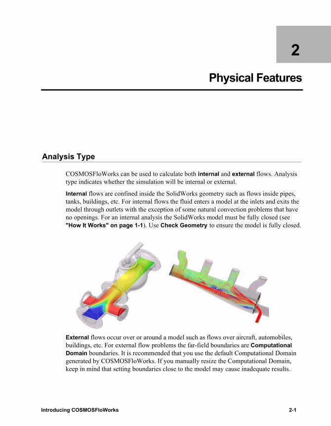
COSMOSFloWorks can be used to calculate both internal and external flows. Analysis type indicates whether the simulation will be internal or external.
Internal flows are confined inside the SolidWorks geometry such as flows inside pipes, tanks, buildings, etc. For internal flows the fluid enters a model at the inlets and exits the model through outlets with the exception of some natural convection problems that have no openings. For an internal analysis the SolidWorks model must be fully closed (see "How It Works" on page 1-1). Use Check Geometry to ensure the model is fully closed.
External flows occur over or around a model such as flows over aircraft, automobiles, buildings, etc. For external flow problems the far-field boundaries are Computational Domain boundaries. It is recommended that you use the default Computational Domain generated by COSMOSFloWorks. If you manually resize the Computational Domain, keep in mind that setting boundaries close to the model may cause inadequate results.
Introducing COSMOSFloWorks 2-1

Chapter 2 Physical Features
Both external and internal flows can be analyzed simultaneously in a COSMOSFloWorks project such as flow around and through a building. If the analysis includes internal and external flow you must specify External type for the analysis.
Before beginning the calculation, COSMOSFloWorks analyzes the SolidWorks model and identifies all inner cavities. Each of these cavities is considered as a flow region and a computational mesh is constructed inside the cavities. For complex models with internal spaces that are not involved in the flow analysis, you can reduce computational resource requirements using one of two options. Both options avoid unnecessary mesh refinements and flow calculations in non-analyzed model regions. The two options are:
• Exclude internal spaces. Use this option for external flow analyses with closed internal spaces that you wish to exclude from the analysis.
• Exclude cavities without flow conditions.This option applies to both internal and external flow analyses. The option is useful for closed internal spaces with no Boundary Conditions or Fans specified on their surfaces.
If you select either of the two options, COSMOSFloWorks will fill the cavities with a solid.
COSMOSFloWorks also allows you to perform two-dimensional calculations. To do this you can select 2D plane flow in the Computational Domain dialog box.
Heat Conduction in Solids
COSMOSFloWorks automatically considers heat transfer within the fluid and between walls and the fluid (convection). By default, COSMOSFloWorks will not consider heat exchange through solids (conduction), but you can enable this capability. The combination of convection and conduction heat exchange, known as conjugate heat transfer, is enabled in the Wizard or General Settings. You should assign the most common solid material in your model as the default material and specify default initial solid temperature. The other materials and initial temperature can be assigned to model components (part or subassembly components in assemblies, as well as bodies in multibody parts) using the Solid Material and Local Initial Condition dialog boxes.
2-2

In case of an External analysis, you do not have to specify Default wall thermal condition on any solid surfaces when a conjugate heat transfer problem is considered. All solid surfaces not in contact with fluid or with another solid are considered as heat-insulated (adiabatic) by default. However, in case of an Internal analysis with heat conduction in solids enabled, you must specify Default outer wall thermal condition under Wall Conditions in the Wizard or General Settings dialog box.
You can also specify surface heat sources at selected solid surfaces (model faces), as well as volume heat sources in the selected solid component. See "Heat Sources – Basic Information" on page 3-9.
To enable heat conduction in solids:
1 Click FloWorks, General Settings and select the Heat conduction in solids option.If no fluid region exists in your heat transfer analysis, you can select the Heat conduction in solids only option.
2 Select Solids on the Navigator pane and define the default solid material.3 Under Initial (Initial and Ambient for external analyses) Conditions, select Solid
parameters to define the initial solid temperature.
You can also enable heat conduction in solids during the project creation in the Wizard, Analysis Type dialog.
Time - Dependent Analysis
COSMOSFloWorks solves the time-dependent form of the Navier-Stokes equations. For steady flow problems COSMOSFloWorks starts the calculation from initial conditions defined by the user. The solver iterates („time-marches“) on the variables until there is no appreciable change, i.e. the solution converges. You can facilitate shorter computation times by specifying initial conditions that are close to the final results. Although this practice is recommended, it is not usually required. For External problems the initial conditions will be the Ambient Conditions of the undisturbed fluid stream around the body.
For unsteady (Transient, or Time-dependent) problems COSMOSFloWorks „time marches“ the solution from initial conditions for the problem’s physical time that you specify. Unlike steady flow problems, the initial conditions must be precise, with the exception of unsteady problems, which have a steady periodic solution (e.g. in the case of periodic boundary conditions) that can be obtained from arbitrary initial conditions, but additional time will be required to eliminate the influence of specified initial conditions.
Steady-state problems are solved by marching the solution in time using time steps determined locally, i.e. at each computational mesh cell independently, which are based on the fluid flow properties of each cell. By default, the time step for solving time-dependent fluid flow problems is specified by COSMOSFloWorks automatically, based on the fluid flow properties only. If you want either to better resolve a problem’s time-dependent solution (by specifying a smaller time step than the automatically selected one, e.g. for
Introducing COSMOSFloWorks 2-3

Chapter 2 Physical Features
resolving periodic solutions of too small period) or to calculate a heat transfer in solids faster (by specifying a larger time step than the automatically selected one, e.g. if the fluid flow does not changed), it is expedient to specify the time step manually. If you solve a time-dependent problem with heat transfer in solids only, i.e., without calculating a fluid flow (the Heat conduction in solids only option is enabled) a manual specification of the time step is preferable.
You can enable the Time-dependent option and specify the Total analysis time and the Output time step in the Analysis Type dialog box of the Wizard. Alternatively, after passing the Wizard, you can enable the Time-dependent option in General Settings and specify the Maximum physical time for finishing the calculation (see "Finishing the Calculation" on page 23-2), as well as strategy and moments of saving results during calculation (see "Saving Results" on page 23-6) in the Calculation Control Options dialog box. To specify time-dependent boundary conditions, use the Dependency dialog box.
See also "Initial Conditions – Basic Information" on page 3-4.
Fluid Type and Compressibility
COSMOSFloWorks simulates flows of incompressible liquids (including non-Newtonian liquids), compressible liquids (liquid density is dependent on pressure), compressible gases or steam (two-phase flows cannot currently be solved by COSMOSFloWorks).
In either the Wizard or the General Settings dialog boxes you specify the Fluid type (gas, liquid, non-Newtonian liquid, compressible liquid or steam) and the substances to be analyzed in the COSMOSFloWorks project.
With COSMOSFloWorks you can analyze a problem involving fluids of different types by defining specific fluid regions as Fluid Subdomains (see "Creating a Fluid Subdomain" on page 8-1). For each fluid subdomain you can assign its own fluid type and the set of fluids. Fluid subdomains must be separated from each other by solid regions.
If your project deals with a high Mach number gas flow, where the Mach number maximum value exceeds about 3 for steady-state or 1 for transient analyses, select the High Mach number flow option in the Default Fluid dialog box of the Wizard or in the Fluids dialog box of the General Settings. COSMOSFloWorks will give you a warning message if your initial (or ambient conditions for External problems) or boundary conditions indicate high velocity flow. During the calculation COSMOSFloWorks will also inform you whether the flow can be considered as a high Mach number gas flow or as a low Mach number gas flow (see "Information and Warnings" on page 25-3). Be aware that if you consider High Mach number flow for low-velocity gas flow (maximum M < 1.5) then solution accuracy may decrease.
2-4
Gravitational Effects
For natural convection problems, include gravitational effects by selecting the Gravity check box in the Wizard or the General Settings dialog box. You should also define the acceleration vector for gravity by specifying the corresponding x, y and z components.
For liquids, check to see that their densities specified in the Engineering Database depend on fluid temperature.
For gases, gravitational effects are available only when the High Mach number flow check box is not selected.
If gravitational effects are considered, the Pressure potential check box is selected by default. When the Pressure potential check box is selected, the specified static pressure is assumed to be piezometric pressure (or potential) and the absolute pressure (Pabs) is reckoned through the reference density, gravitational acceleration vector and the position vector:
,
where gi - component of the gravitational acceleration vector and x,y,z – coordinates in the global coordinate system. When the Pressure potential check box is clear, the specified static pressure is assumed to be an absolute pressure, and the corresponding piezometric pressure is respectively reckoned.
If you have a part, you can easily change the location of the global coordinate system’s origin by creating an assembly from this part. To display the global coordinate system, right-click the project name at the top of the COSMOSFloWorks analysis tree and select Show Global Coordinate System.
Turbulence
COSMOSFloWorks solves turbulent flow problems by default. However you can turn off turbulence by selecting the Laminar Only flow in the Wizard or General Settings dialog box. Turbulence is normally found in the bulk of the flow field and also in the boundary layers near walls.
If you have not specified Laminar Only or Turbulent Only flow, the flow can be either laminar or turbulent or with transition from one type to another (depending on the flow characteristics).
Default turbulence parameters are defined by COSMOSFloWorks. The turbulence parameters may be manually specified in terms of turbulent intensity and turbulent length or in terms of turbulent energy and turbulent dissipation. For most flows it is difficult to have a good estimation of the turbulence a priori so it is recommended that the default turbulence parameters be used. The turbulence parameters are specified for initial conditions, inlet boundary conditions, or as ambient conditions in external problems. Additionally, boundary layer parameters at the model walls at inlets are always specified by default by COSMOSFloWorks.
( )specified piezo abs x y zP P P g x g y g zρ= = − + +
Introducing COSMOSFloWorks 2-5

Chapter 2 Physical Features
The default boundary layer type is determined inside COSMOSFloWorks from the Reynolds number defined on the
equivalent hydraulic diameter ( , where A is the opening cross section area, P is
the perimeter of the opening). The layer thickness is determined from the effective wall length also governed by this Reynolds number. In the Boundary Condition dialog box you can specify the boundary layer parameters by clicking the Show advanced parameters check box on the Settings tab. Here it is possible for you to specify a laminar or turbulent (if you have not specified Laminar Only flow) boundary layer and its thickness.
See "Overview of Conditions" on page 3-1 for additional information about initial, ambient and boundary conditions.
Porous Media
If the SolidWorks model is an assembly (or multibody part), COSMOSFloWorks is able to treat some of its components as porous media with the fluid flow through them, simulating them as fluid cavities with a distributed resistance to fluid flow. The fluid flow through a porous body depends on the porous medium’s properties and on the outer flow’s conditions. To facilitate your work, COSMOSFloWorks offers you wide capabilities of specifying porous medium properties. First of all, in the Engineering Database, specify effective porosity of the porous medium, defined as the volume fraction of the interconnected pores with respect to the total medium volume. Then select the porous medium’s permeability type from the following ones:
• Isotropic - the medium permeability is independent of direction within the medium• Unidirectional - the medium is permeable in one direction only• Axisymmetrical - the medium permeability is fully governed by its axial (n) and
transverse (r) components with respect to a specified direction• Orthotropic - the general case, when the medium permeability varies with direction
and is fully governed by its three components determined along three principal directions.
Then specify the medium’s permeability (its components, if it is axisymmetrical or orthotropic) in the form of the medium resistance to fluid flow (Resistance calculation formula), k, which is defined as k = - grad(P)/(ρ·V), where P, ρ, V are, accordingly, fluid pressure, density, and velocity. You can specify the k vector components with one of the following two formulas:
• k = ∆P·S/(m·L) (named Pressure Drop, Flowrate, Dimensions), where ∆P is the pressure difference between the opposite sides of a parallelepiped porous body, m is the mass flow rate through the body, S and L are, accordingly, the body cross-sectional area and length, all in the selected direction. You specify ∆P as a function of m, whereas S and L as constants. Instead of mass flow rate you can specify
D 4AP
-------=
2-6

volume flow rate, v, in this case COSMOSFloWorks calculates m = v·ρ. In addition, since the porous medium resistance coefficient k at the specified pressure drop ∆P or mass flow rate m is usually proportional to the fluid's dynamic viscosity and the parameters denoting k has been determined with another (than in the current project) fluid (let us name it calibration fluid), you can correct k for the project fluid by specifying this calibration fluid's non-zero dynamic viscosity, which here is named Calibration viscosity, µcal. As a result, k will be determined as k = ∆P·S·m/(m·L·µcal), where µ is the project fluid's dynamic viscosity.All these values do not specify the porous body inserted into the SolidWorks model under consideration, but specify the porous medium property. COSMOSFloWorks automatically scales k to the porous body inserted into the model in accordance with its dimensions.
• k = (A·V+B)/ρ (named Dependency on velocity), where V is the fluid velocity, A and B are constants. You specify A[kg/m4] and B[kg/(s×m3)] only (V and r are calculated).
The following two formulas are used to specify the resistance of a porous medium consisting of long narrow channels. This type of medium resistance combined with the Unidirectional permeability type allows you to simulate fluid flow through arrays of tightly packed parallel thin tubes.
• k= 32µ/(ε·ρ·D2) (named Dependency on reference pore size (D)), where m and ρ are the fluid dynamic viscosity and density, D is the reference pore size determined experimentally, ε - porosity. You specify D only (µ and ρ are calculated). This dependency should be used if you consider a fluid flow in each of the porous medium's narrow channels as laminar.
• k= µ/(ρ·D2)·f(Re) (named Dependency on reference pore size (D) and Reynolds number), differing from the previous formula by the f(Re) factor, yielding a more general formula. Additionally to D, you specify f(Re) as a formula dependency. Use this dependency if you consider a fluid flow in each of the porous medium's narrow channels as turbulent.
In the Porous Medium dialog box, specify the rest of the data, determining the porous body inserted into the model:
• the porous medium from the Engineering Database,• the model components, to which the porous medium is applied,
For admissible resistance values the following limitation exists: k must be
less than , where V and x are the fluid velocity and the maximum
cell size inside the porous medium respectively. Otherwise, the results may be incorrect. If you exceed this limitation you must decrease x by refining the mesh inside the porous medium, especially at the porous/fluid interface.
xV100
Introducing COSMOSFloWorks 2-7

Chapter 2 Physical Features
• if a medium’s permeability type is unidirectional or axisymmetrical, then you need to specify the direction (axial direction for an axisymmetric porous medium) as an axis of the selected coordinate system or as a selected curve, to which the direction is tangent.
Water Vapor Condensation
If you specify that the project’s gaseous fluid (i.e. gas) includes water vapor (i.e. steam), COSMOSFloWorks can predict an equilibrium volume condensation of water from the water vapor (any surface condensation is not considered). As a result of this prediction, in accordance with the fluid’s local temperature and pressure and, if a multi-component fluid is considered, the water vapor’s local mass fraction, the condensed water vapor’s local mass fraction in the local total mass of the water vapor and the condensed water vapor is determined. In addition, the corresponding changes of the fluid’s temperature, density, enthalpy, specific heat, and sonic velocity are determined and taken into account when determining the fluid’s properties. Since the employed condensation model is at full equilibrium, the condensed water vapor has no history, i.e. it is a local fluid property only.
In order for this simplification to be valid, the condensation prediction is based on the assumption that the condensed water’s volume is equal to zero. As a result, this prediction is correct only in those cases when the predicted condensed water’s relative volume does not exceed 5%. In addition, this prediction is valid in the water vapor’s temperature range of 283...610 K and pressure range up to 107 Pa. If these restrictions are violated, the user is informed by COSMOSFloWorks with a corresponding warning in the solver monitor window.
Non-Newtonian Liquids
COSMOSFloWorks is capable of calculating the laminar flow of inelastic non-Newtonian liquids. All available non-Newtonian models are based on the assumption that the flow’s shear stress (τ) is a function of the flow’s shear rate ( ): , or, introducing the liquid’s dynamic viscosity (η) similarly to Newtonian liquids, . The following three models of inelastic non-Newtonian viscous liquids are available:
The Herschel-Bulkley model. , where K is the liquid’s consistency coefficient ( ), n is the liquid’s power-law index (dimensionless), and το is the liquid’s yield stress (Pa). This model includes the following special cases:
• n = 1, τo = 0 describes Newtonian liquids, in this case K is the liquid’s dynamic viscosity;
• n = 1, τo> 0 describes the Bingham model of non-Newtonian liquids, featured by a non-zero yield stress (τo), below of which the liquid behaves as a solid, so to achieve a flow this threshold shear stress must be exceeded (this threshold is
γ& ( )γτ &f=( ) γγητ && ⋅=
( ) onK τγτ +⋅= &
nsPa ⋅
2-8

modeled by automatically equating K, named plastic viscosity in this case, to a substantially high value at τ < τo);
• 0 < n < 1, τo = 0 describes the power-law model of shear-thinning non-Newtonian liquids;
• n > 1, τo = 0 describes the power-law model of shear-thickening non-Newtonian liquids.
The power-law model. , i.e., , in contrast to the above-mentioned Herschel-Bulkley model special case, the η values are restricted: ηmin ≤ η ≤ ηmax, so these minimum and maximum dynamic viscosities (Pa⋅s) are specified in addition to consistency coefficient K ( ) and power-law index n (dimensionless);
The Carreau model. , , where η∞ is the liquid’s dynamic viscosity at an infinite shear rate, i.e., the minimum
dynamic viscosity (Pa⋅s), ηo is the liquid’s dynamic viscosity at zero shear rate, i.e., the maximum dynamic viscosity (Pa⋅s), K1 is the time constant (s), n is the power-
law index (dimensionless). This model is a smooth version of the power-law model with the above-mentioned η restrictions.
In the models mentioned above all parameters, with the exception of the dimensionless power-law index, can be specified temperature-dependent.
If several (n) non-Newtonian liquids mix, their mixture’s dynamic viscosity is determined from the following formula:
,
where yi and µi - mass concentration and dynamic viscosity of the mixture’s i-th component. Note that this formula may be not applicable for mixtures of specific non-Newtonian liquids.
Compressible Liquids
A liquid density is specified in the Engineering Database as either a constant or a tabular dependence on temperature under the Liquids item. Additionally, under the Compressible liquids item you can specify a dependence of the liquid density on pressure ρ (P), i.e., the liquid’s compressibility, through one of the following forms of the Tait equation of state:
, where ρ0 is the liquid’s density under the reference
( )nK γτ &⋅= ( ) 1−⋅= nK γη &
nsPa ⋅
γητ &⋅= ( ) ( )[ ]( ) 2/1211
−
∞∞ ⋅+⋅−+=n
o K γηηηη &
mixµ
( )∑=
=n
iiimix logylog
1µµ
00
/ 1 ln B PCB P
ρ ρ +
= − ⋅ +
Introducing COSMOSFloWorks 2-9

Chapter 2 Physical Features
pressure P0, C and B are coefficients, (ρ0, C, B, and P0 are specified by the user as constants or, except for P0, as tabular dependences on temperature), P is the calculated pressure;
, where, n is a power index specified by the user as a constant
or a tabular dependence on temperature.
If several (n) compressible liquids mix, their mixture’s parameters (dynamic viscosity, density, etc.) is determined from the following formula:
,
where yi - mass concentration and Ai - parameter of the mixture’s i-th component. Note that this formula may be not applicable if parameters of mixing liquids vary considerably.
Surface-to-surface Radiation
If you solve a problem including heat conduction in solids, in which a solid’s temperature is too high and/or the gas is too rarefied, so that heat transfer by radiation from and/or between solids is noticeable with respect to heat transfer by convection (i.e. heat radiation from the solid surfaces and/or to them plays an important role in the problem, noticeably influencing the solids’ temperature) you have the option to activate the Radiation physical feature and specify the solid surfaces’ emissivity. In addition, if required by the problem’s statement, you can specify heat radiation from the computational domain’s far-field boundaries (or the model’s openings) into the computational domain (into the model) through the boundaries’ emissivity and temperature values. As a result, this radiative heat acts upon the model’s walls and can heat them.
The following standard (FW-Defined) surfaces are available in the Engineering Database:
• Solar opening denotes a surface, which radiates heat (as directional radiation) into the model along the Direction (defined by the X, Y, Z components of the direction vector) and with the Intensity specified in the Radiative surface dialog box. For time-dependent analyses, the solar radiation condition can be specified as a function of time by clicking Dependency,
• Symmetry. If you use the Ideal Wall condition at a wall to specify the problem’s symmetry plane, the Symmetry radiative surface type should be specified at this wall if the surface-to surface radiation is considered in the problem,
• Non-radiating surface denotes that this surface does not participate in the radiation heat transfer, i.e. neither emits nor absorbs heat radiation,
• Blackbody opening/outer boundary denotes that the surface’s emissivity is equal to 1 (the blackbody one), so this surface radiates heat into the computational domain (into the model) as a blackbody, and that its temperature is not calculated, but specified by you in the Radiative temperature box of the Radiative surface dialog
1/
00
nP BP B
ρ ρ +
= ⋅ +
( )∑=
=n
iiimix AyA
1loglog
2-10
box, which appears if the Blackbody opening/outer boundary type of radiative surface is selected,
• Absorbent wall denotes that the surface fully absorbs all the incident radiation falling upon it, i.e. as a blackbody, but in contrast to it, does not radiate any heat (i.e., no rays start from it),
• Blackbody wall denotes that the surface’s emissivity is equal to 1 (the blackbody one), i.e., the wall surface fully absorbs all the incident radiation falling upon it and emits the heat in accordance with the Stefan-Boltzmann law,
• Whitebody wall denotes that the surface’s emissivity is equal to 0 (the whitebody one), i.e., the wall surface fully reflects all the incident radiation (in accordance with the Lambert law) and does not emit any heat by itself, so the surface temperature does not affect the heat radiation,
At the computational domain’s far-field boundaries you can specify the following radiative conditions by selecting corresponding check boxes in the Analysis type dialog box of the Wizard or General Settings:
• Environment radiation. The Environment radiation can be specified for both external and internal analyses. It denotes that the computational domain’s far-field boundaries radiates heat (Q) into the computational domain using the Emissivity coefficient (ε = 1, specified in the Engineering Database under the Radiative Surface, FW Defined, Blackbody opening/outer boundary item) and the specified Environment temperature as shown below:Q = ε σT4.
• Solar radiation. Select this check box to enable directional radiation from ambient space and specify the directional vector (using the X, Y, Z components of the direction vector) and the Solar Intensity.
A custom radiative surface is defined thought the Emissivity coefficient and one of the following Radiative surface types:
• Wall. Denotes a surface which radiates heat with emissivity specified by you in the Emissivity coefficient box (in the range from 0 to 1, i.e., a gray-body emissivity can be specified).
• Opening/Outer boundary. Denotes a surface which radiates heat into a model with emissivity specified by you in the Emissivity coefficient box (in the range from 0 to 1). At that, the surface’s temperature is not calculated, but specified by you in the Radiative temperature box of the Radiative surface dialog box, which appears if the Opening/outer boundary type is selected.
• Wall to ambient. Denotes a surface which radiates heat with emissivity specified by you in the Emissivity coefficient box (in the range from 0 to 1), but this heat does not arrive at the model’s walls, i.e., disappears in the surrounding space (as a result, the radiation rays from this surface are not calculated).
When viewing the calculation results, you can visualize the following radiation characteristics:
Introducing COSMOSFloWorks 2-11
Chapter 2 Physical Features
• the local characteristics (power per unit area) in Surface Plots (when selecting Fluid as medium): the Net radiant flux (the difference of the radiant flux leaving the surface at this point and the one arriving at it, so it is positive if the leaving flux is greater than the arriving one) and the Leaving radiant flux (the radiant flux leaving the surface);
• the integral characteristics (power) among the integral Surface Parameters: the Net radiation rate (the net radiant flux integrated over the selected surface) and the Leaving radiation rate (the leaving radiant flux integrated over the selected surface).
You can specify some of the solid bodies in the model as transparent for the radiative heat transfer. See "Specifying Components Transparent for the Heat Radiation" on page 5-8.
Compressible Flows
Flows are considered compressible if the fluid density depends on pressure so density change effects are important.
In COSMOSFloWorks, gases are always compressible and liquids can be incompressible or compressible. If your project deals with a high-velocity gas flow, where the Mach number maximum value exceeds about 3 for steady-state analyses or 1 for transient (time-dependent) analyses, you should consider the gas flow as a high Mach number flow. To consider high Mach number gas flow, select the High Mach number flow check box either in the Wizard or General Settings.
• In all cases, the project fluids neither emit nor absorb heat radiation (i.e., they are transparent to heat radiation), so the considered heat radiation concerns solid surfaces only.
• The radiative solid surfaces which are neither blackbody nor whitebody are assumed ideal gray-body, i.e. having a continuous emissive power spectrum similar to the blackbody one, so their monochromatic emissivity is independent of the emission wavelength. The total radiation integrated over all wavelengths is considered only. For certain materials with certain surface conditions (some of them are available from the Radiative Surface tab of the Engineering Database), the gray-body emissivity can depend on the surface temperature only.
• In all the cases, the heat radiation from the solid surfaces is assumed diffuse, i.e. obeying the Lambert law, according to which the radiation intensity per unit area and per unit solid angle is the same in all directions.
• The net radiation heat exchange between the model’s radiative surfaces is calculated along with the convective heat transfer and the heat transfer in solids.
2-12
The low Mach number gas flow is recommended for the tasks where the supersonic flow is localized in relatively small fluid volume and the major flow is subsonic. If the fluid volume in which the flow becomes supersonic is about a half of the computational domain size or greater, it is recommended that you consider the flow as a high Mach number gas flow.
Incompressible Flows
Flows are considered incompressible if the fluid density depends only on temperature and concentration so density change effects are negligible.
Basic Mesh
The basic mesh is constructed for the whole computational domain at the beginning of the meshing process. It is formed by dividing the computational domain into slices by parallel planes which are orthogonal to the Global Coordinate System’s axes. The computational domain’s boundary planes (at X min, … Z max) are among these planes.
By default, the basic mesh’s planes are spaced in the X-, Y-, and Z-directions of the Global Coordinate System nearly uniformly, and the distances between them are determined from the specified numbers of cells in these directions (Nx, Ny, Nz). If necessary, you can insert additional mesh planes and specify another spacing between them (i.e., non-uniform steps) by creating the Control Planes.
Travel
The term travel, used together with iterations is a unit characterizing the calculation duration. We denote the calculation period (in its turn, it can be measured in iterations or in another unit) required for a flow disturbance to cross the computational domain’s fluid region. So, value N travels denotes the calculation period required for a flow disturbance to cross the computational domain N times. The travel equivalent in iterations is determined just after starting the calculation and can be seen in the Info box while monitoring the calculation.
Partial Cells
A partial cell is a computational mesh cell lying at the solid/fluid interface, partly in a fluid region and partly in a solid region.
Introducing COSMOSFloWorks 2-13
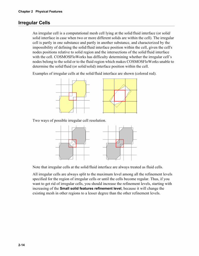
Chapter 2 Physical Features
Irregular Cells
An irregular cell is a computational mesh cell lying at the solid/fluid interface (or solid/solid interface in case when two or more different solids are within the cell). The irregular cell is partly in one substance and partly in another substance, and characterized by the impossibility of defining the solid/fluid interface position within the cell, given the cell's nodes positions relative to solid region and the intersections of the solid/fluid interface with the cell. COSMOSFloWorks has difficulty determining whether the irregular cell’s nodes belong to the solid or to the fluid region which makes COSMOSFloWorks unable to determine the solid/fluid (or solid/solid) interface position within the cell.
Examples of irregular cells at the solid/fluid interface are shown (colored red).
Two ways of possible irregular cell resolution.
Note that irregular cells at the solid/fluid interface are always treated as fluid cells.
All irregular cells are always split to the maximum level among all the refinement levels specified for the region of irregular cells or until the cells become regular. Thus, if you want to get rid of irregular cells, you should increase the refinement levels, starting with increasing of the Small solid features refinement level, because it will change the existing mesh in other regions to a lesser degree than the other refinement levels.
2-14

3 Conditions and Tools
Overview of Conditions
Any problem solved with COSMOSFloWorks must have initial conditions and boundary conditions. In steady state problems, initial conditions influence the rate of convergence to the steady state, whereas boundary conditions fully govern the flow pattern. In transient (unsteady) problems the time-dependent flow pattern depends both on initial conditions and boundary conditions.
• You specify flow initial conditions in the Wizard or General Settings dialog box using different names: Initial and ambient Conditions for External flows and Initial Conditions for Internal flows.
• Within a closed fluid region or volume of model's component you can specify Initial Conditions different from the default ones (specified in the Wizard or General Settings dialog box). The closed fluid region can be selected by selecting one of the faces bounding it. If you want to use a component of an assembly (or a body in a multibody part) to define a fluid region, you must disable the component either in the Component Control dialog box (see "Component Control" on page 5-7) or by selecting the Disable solid components option in the Local Initial Condition dialog box (see "Initial Conditions" on page 19-1).
• If you consider Heat Conduction in Solids, you specify the initial solid temperature in the Wizard or General Settings.
• In an assembly (or in a multibody part) you can specify a component initial solid temperature that is different from the default (see "Initial Conditions" on page 19-1) solid temperature condition. For internal flows we recommend to create the lids used to close the openings as separate components. Then you can specify a material with zero thermal conductivity (insulator) for the lid components. This will prevent heat transfer in the lid components.
• You can use results of the previous calculation performed either in the current project or other projects, as the initial conditions for the newly prepared calculation.
Introducing COSMOSFloWorks 3-1

Chapter 3 Conditions and Tools
In the Wizard or General Settings you can apply any available results by selecting Transferred initial conditions. See "Initial and Ambient Conditions" on page 6-10. To apply the current project's results as initial conditions for a new project calculation you can also use the Take previous results option. See "Running the Calculation" on page 24-1.
You can specify flow boundary conditions somewhat differently for External and Internal flows:
• For External flows you specify flow boundary conditions at all of the Computational Domain boundaries (as either ambient or symmetry conditions) and, if necessary, at the model surfaces among which there can be Openings.
• For Internal flows you specify flow boundary conditions at inner model surfaces and, if necessary, at the Computational Domain boundaries (as symmetry conditions).
Specification of boundary conditions at the Computational Domain boundaries:
• Specification at the Computational Domain boundaries is performed through the Wizard or General Settings dialog box with the ambient conditions values.
• (PE ONLY) You can also specify boundary conditions at the Computational Domain boundaries inside the model by using the Transferred Boundary Condition dialog box.
• You can specify Symmetry boundary conditions on the Computational Domain boundaries that coincide with the flow symmetry planes. See "Computational Domain" on page 7-1.
• For analyses with radiation, you can specify heat radiation from the computational domain's far-field boundaries into the computational domain by specifying an Environment radiation in the Wizard or General settings.
Specification of boundary conditions on model surfaces:
• The inlet and outlet flow boundary conditions are specified on the model surfaces in contact with the fluid in the Boundary Condition dialog box.
• If there is a fan in your model, the fan condition is also specified on the model surface in contact with the fluid in the Fun dialog box.
• Heat sources on solid surfaces in the form of Heat Transfer Rate, Heat Flux (if “Heat conduction in solids” is not considered) and in the form of Heat Generation Rate, Surface Heat Generation Rate (if “Heat conduction in solids” is under consideration) are specified in the Surface Source dialog box.
• In the Wizard or General Settings you specify thermal wall boundary conditions on all solid surfaces in contact with the fluid (see "Default Wall Conditions" on page 6-7).
• If you consider Heat Conduction in Solids, the thermal wall boundary conditions are not required. Instead, a conjugate heat transfer problem is solved at the boundary between the fluid and the solid.
3-2

• In the Boundary Condition dialog box you can specify a Real Wall boundary condition for selected solid surfaces in contact with the fluid. The Real Wall condition allows you to specify the wall Roughness and/or wall Temperature and/or Heat transfer coefficient at the model surfaces.
• The Real Wall condition also allows you to specify a tangential velocity boundary condition at a wall to simulate translation and/or rotation of the wall. In addition, the stator motion type can be specified to define a non-rotating wall in case a rotating frame of reference is enabled.
• In the Boundary Condition dialog box you can specify an Ideal Wall condition for selected solid surfaces in contact with the fluid. An Ideal Wall condition corresponds to an adiabatic, frictionless surface. Specifying an Ideal Wall condition allows you to use the surface as a flow symmetry plane where applicable for reducing computational resources. This option is available for both internal and external analyses.
• For analyses with “Heat conduction in solids” you can also specify thermal wall condition on outer model walls, which are not in contact with the project’s fluid but inside the computational domain. This condition allows you to define heat exchange between the external flow and the outer model walls for internal analysis. The default thermal condition applied to all of the model walls is specified in the Wizard or General Settings dialog box and can be adjusted for a specific wall by creating an Outer Wall boundary condition.
• The Transferred Boundary Condition allows you to use results of a previous calculation (may be performed in another project) as a boundary condition on a selected model surface.
• If your project includes radiation, you can specify heat radiation from the model opening into the model by applying the Blackbody opening/outer boundary radiative surface to the opening surface. See "Creating a Radiative Surface" on page 15-1.
• For internal analyses with radiation, you can specify the radiative heat exchange between the model outer walls and the ambient space by specifying the Default outer radiative surface in the Wizard or General settings dialog box or by creating the Radiative Surface condition at a specific wall.
Specification of boundary conditions in a local region:
• You can specify heat source in a local solid or fluid region in the form of Heat Generation Rate, Volumetric Heat Generation Rate or Temperature in the Volume Source dialog box.
You can use the following helpful options for data input:
• The Dependency button in the data specification dialog boxes allows you to specify data as follows: as a constant, as tabular or formula dependency on X, Y, Z, r, θ, ϕ coordinates and time t (for time-dependent analyses only). The θ, j and r coordinates allow you to specify parameters in a spherical coordinate system. In a cylindrical coordinate system, radius r is reckoned from the Reference axis. You specify the
Introducing COSMOSFloWorks 3-3
Chapter 3 Conditions and Tools
reference axis as an axis of a selected Cartesian coordinate system (Global Coordinate System in Wizard and General Settings).
• The Units database (the part of the Engineering Database) allows you to specify data in a suitable unit system. You can assign a default unit system in the Unit System dialog box (accessible by clicking FloWorks, Units) or in the Wizard. Note that COSMOSFloWorks allows you to enter values in any other standard or user defined unit system. If you choose to enter data that are not in default units, you must type the appropriate numerical value and unit symbols. For instance: instead of 26.85 °C you could enter 300 K. COSMOSFloWorks will automatically translate the value into the project’s default unit system.
Initial Conditions – Basic Information
Any steady state flow problem is initially considered as a time-dependent problem and solved as a transition by time steps (in this case, as iterations) from a specified initial flow state to a steady state flow. Therefore, initial flow conditions, i.e., initial distributions of independent flow parameters (see below) must be specified over the computational domain. If you want to solve an Internal problem in a shorter time, simply specify initial conditions closer to the assumed solution (instead of using the default values). If you solve an External problem, you specify initial conditions as Initial and ambient conditions. Ambient conditions are values of the undisturbed external flow’s independent parameters. If you solve a time-dependent problem, you specify initial conditions exactly for the start time, with the exception of unsteady problems, which have a steady periodic solution (e.g. in the case of periodic boundary conditions). The solution can be obtained from arbitrary initial conditions, but additional time will be required to eliminate the influence of the specified initial conditions.
You specify flow initial conditions data in Wizard or General Settings as values of independent flow parameters in the following possible combinations:For gases:
• Static pressure, static temperature, and velocity• Static pressure, static density, and velocity• Static temperature, static density, and velocity
For liquids:• Static pressure, temperature, and velocity
For gases you can specify Mach number instead of the absolute velocity (see "Fluid Type and Compressibility" on page 2-4).Additionally, you can specify one of the following two combinations of Turbulence parameters:
• Turbulent intensity and turbulent length
• Turbulent energy and turbulent dissipation
3-4

If you consider Heat Conduction in Solids you specify the default Initial solid temperature in the Wizard or General Settings dialog box.COSMOSFloWorks sets default values for all these parameters automatically. Although you can change any of these parameters, we recommend the defaults if you are not fully confident in your assumed values. As a result of all these settings, COSMOSFloWorks imposes the specified flow and solid parameter values by default throughout the fluid and solid region.
You can create a project that includes internal flow regions with initial conditions that are different from the defaults. The Local Initial Condition dialog box allows you to select a closed fluid region to apply the initial conditions by selecting one of the faces bounding the region. Also, the flow regions (not only closed ones) can be simulated using separate component parts, which may require you to create an assembly. You can use a Top-down assembly technique to insert a new component inside the flow field. Next, disable the component using Component Control, so that COSMOSFloWorks treats it as a fluid. If a fluid component overlaps the solid region, COSMOSFloWorks considers the overlapped region as a solid. To specify the initial conditions in the component treated as a fluid, use the Local Initial Condition dialog box.In an assembly you can specify a component initial solid temperature that is different from the default (see "Creating an Initial Condition" on page 19-1). For internal flows we recommend to create the lids used to close the openings as separate components (parts). Then you can specify a material with zero thermal conductivity for the lid components. This will prevent heat transfer in the lid components.
You can use the results of the previous calculation performed either in the current project or other projects as the initial conditions for the newly prepared calculation. In the Wizard or General Settings dialog box you can apply any available results by selecting Transferred initial conditions. See "Initial and Ambient Conditions" on page 6-10. To apply the current project’s results as initial condition for the new project calculation you can also use the Take previous results option.
Boundary Conditions – Basic Information
Any problem solved with COSMOSFloWorks must have boundary conditions. Boundary conditions fully govern the steady-state flow pattern, whereas a time-dependent flow pattern depends on both boundary conditions and initial conditions.
You specify flow boundary conditions somewhat differently for External and Internal flows:
• For External flows you specify flow boundary conditions at all of the Computational Domain boundaries (as either ambient or symmetry conditions) and, if necessary, at the model surfaces among which there can be Openings.
• For Internal flows you specify flow boundary conditions at inner model surfaces, both walls and Openings and, if necessary, at the Computational Domain boundaries (as symmetry conditions).
Introducing COSMOSFloWorks 3-5

Chapter 3 Conditions and Tools
Specification of boundary conditions on the Computational Domain boundaries:
• As Initial and ambient conditions for External flows in Wizard or General Settings.
• (PE ONLY) As Ambient, or Velocity, or Impulse, or Static pressure, or Total pressure boundary conditions on the selected computational domain boundaries for both Internal and External flows by taking results of another calculation with the Transferred Boundary Conditions wizard. If Heat Conduction in Solids is enabled and the selected computational domain boundary lies partly (or fully) in a solid, then the solid temperature at this boundary part is taken as the solid boundary condition. Whereas the heat flux is obtained as the problem’s solution at this boundary and depends on the heat transfer in solid.
• As flow Symmetry conditions at the flow symmetry planes (coinciding with the computational domain boundaries) for both Internal and External flows by using the Computational Domain dialog box.
• For analyses with radiation, you can specify heat radiation from the computational domain’s far-field boundaries into the computational domain by specifying an Environment radiation in the Wizard or General settings.
Specification of boundary conditions on model surfaces:
• The inlet and outlet flow boundary conditions are specified on the model surfaces in contact with the fluid in the Boundary Condition dialog box.
• If there is a fan in your model, the fan condition is also specified on the model surface in contact with the fluid in the Fan dialog box.
• The heat sources on solid surfaces in the form of Heat Transfer Rate, Heat Flux (if “Heat transfer in solids” is not considered) and in the form of Heat Generation Rate, Surface Heat Generation Rate (if “Heat conduction in solids” is under consideration) are specified in the Surface Source dialog box.
• If you do not consider Heat Conduction in Solids, then in Wizard or General Settings you specify thermal wall boundary conditions on all solid surfaces in contact with the fluid (see "Default Wall Conditions" on page 6-7).
• If you consider Heat Conduction in Solids, the thermal wall boundary conditions are not required. Instead, a conjugate heat transfer problem is solved at the boundary between the fluid and the solid.
• In the Boundary Condition dialog box you can specify a Real Wall boundary condition for selected solid surfaces in contact with the fluid. The Real Wall condition allows you to specify the wall Roughness and/or wall Temperature and/or Heat transfer coefficient at the model surfaces.
• The Real Wall condition also allows you to specify a tangential velocity boundary condition at a wall to simulate translation and/or rotation of the wall. In addition, the stator motion type can be specified to define a non-rotating wall in case a rotating frame of reference is enabled.
3-6

• In the Boundary Condition dialog box you can specify an Ideal Wall condition for selected solid surfaces in contact with the fluid. An Ideal Wall condition corresponds to an adiabatic, frictionless surface. Specifying an Ideal Wall condition allows you to use the surface as a flow symmetry plane in relevant cases for reducing computational resources. This option is available for both internal and external analyses.
• For analyses with “Heat conduction in solids” you can also specify thermal wall condition on outer model walls, which are not in contact with the project’s fluid but inside the computational domain. This condition allows you to define heat exchange between the external flow and the outer model walls for internal analysis. The default thermal condition applied to all model walls is specified in the Wizard or General Settings and can be adjusted for a specific wall by creating an Outer Wall boundary condition.
• (PE ONLY) You can also specify inlet and outlet flow boundary conditions on model surfaces by taking results of another calculation with the Transferred Boundary Condition wizard.
• If your project includes radiation, you can specify heat radiation from the model opening into the model by applying the Blackbody opening/outer boundary radiative surface to the opening surface in contact with the fluid. See "Creating a Radiative Surface" on page 15-1.
• For internal analyses with radiation, you can specify the radiative heat exchange between the model outer walls and the ambient space by specifying the Default outer radiative surface in the Wizard or General settings or by creating the Radiative Surface condition at a specific wall.
Specification of boundary conditions in a local region:
• You can specify heat source in a local solid or fluid region in the form of Heat Generation Rate, Volumetric Heat Generation Rate or Temperature in the Volume Source dialog box.
r
When specifying boundary conditions for an internal analysis you must take care of their physical compatibility. For example, a project will not run for internal steady-state flows when at model inlets and outlets you specify boundary conditions of the Flow opening type (or Transferred Boundary Condition of the Velocity type) without any boundary condition of the Pressure opening type, so the inlet and outlet mass flow rates are not balanced exactly. To avoid such problems we recommend that you specify at least one pressure condition (Boundary Condition of the Pressure Opening type or Transferred Boundary Condition of the Static (Total) Pressure type) and at least one Boundary Condition of the Flow Opening type or Transferred Boundary Condition of the Velocity (or Impulse) type.
Introducing COSMOSFloWorks 3-7
Chapter 3 Conditions and Tools
Transferred Boundary Conditions - Basic Information
The Transferred Boundary Conditions allows you to focus on a specific region within your model by using results obtained in a previous COSMOSFloWorks calculation as a boundary condition for the current COSMOSFloWorks project. The only requirement is both the used results and the current project must have the same Global Coordinate System. The Transferred Boundary Condition wizard offers you to pass through the following three steps.
To run the Transferred Boundary Condition wizard, click FloWorks, Insert, Transferred Boundary Condition.
At Step 1 - Selecting Boundaries you select the current COSMOSFloWorks project’s flow boundaries to apply the Transferred Boundary Conditions. You can select them either as Computational domain boundaries (X max, … Z min) or as the project model’s faces (i.e., openings) by selecting them in the graphic area. The first case is relevant for external analyses, whereas the second one is relevant for internal analyses.
r
At Step 2 - Selecting Results to Transfer you select either a COSMOSFloWorks project (from any projects of currently open models) or results file (.fld), whose results will be taken as the transferred boundary conditions for the current COSMOSFloWorks project.
At Step 3 - Specifying Type of Condition you select type of the transferred boundary condition, i.e., a set of the flow field parameters whose values will be transferred from a previous COSMOSFloWorks calculation to the current COSMOSFloWorks project at the selected boundaries. In the Boundary condition type list you can select one of the following types of flow parameters:
• Ambient – the same flow parameters which are specified at the computational domain boundaries in external analyses; during the calculation they act in the same manner, as for external analyses;
• Impulse – the same flow parameters (fluid temperature, density, substance concentrations, and turbulence parameters) which are specified at the computational domain boundaries in external analyses, with the exception of specifying fluid impulse instead of fluid velocity (both are vectors); during the calculation they act nearly in the same manner, as for external analyses;
• Velocity – the same flow parameters (fluid velocity, temperature, density, substance concentrations, and turbulence parameters) which are specified at the computational domain boundaries in external analyses; during the calculation they act nearly in the same manner, as for external analyses;
• Static pressure – the same flow parameters (static pressure, temperature, substance concentrations, and turbulence parameters) which are specified in
The calculation will not run if the Computational Domain is entirely in the solid. There must be at least one fluid cell to run the calculation.
3-8

the Pressure Openings set of boundary conditions when you select the Static Pressure type of this boundary condition; during the calculation they act nearly in the same manner, as a Pressure-Opening-with-Static-Pressure boundary condition;
• Total pressure – the same flow parameters (total pressure, temperature, substance concentrations, and turbulence parameters) which are specified in the Pressure Openings set of boundary conditions when you select the Total Pressure type of this boundary condition; during the calculation they act nearly in the same manner, as a Pressure-Opening-with-Total-Pressure boundary condition.
Independently of the Transferred Boundary Condition type selected from the above-mentioned variants, if the boundary’s section lies in the solid and Heat Conduction in Solids is enabled in the current COSMOSFloWorks project and was enabled in the COSMOSFloWorks project whose results are taken as the transferred boundary condition, then the solid temperature is taken from this project’s results as the transferred solid boundary condition, whereas the heat flux obtained as the problem’s solution at this boundary depends on the heat transfer in this solid, and in particular can be non-zero.r
See also "Creating Transferred Boundary Conditions" on page 12-1.
Heat Sources – Basic Information
You can specify Heat Sources either on a surface (Surface Source), where neither Boundary Conditions (or Transferred Boundary Condition) nor Fans are specified (i.e. through which the fluid does not flow), or in the medium, which can be either solid or fluid (Volume Source).
In Surface Source you can specify heat sources on solid surfaces in the form of Heat Transfer Rate, Heat Flux if “Heat conduction in solids” is not considered, and in the form of Heat Generation Rate, Surface Heat Generation Rate if “Heat conduction in solids” is under consideration (in both cases, a positive value denotes heat generation, a negative value denotes heat absorption).
When specifying boundary conditions for an internal analysis you must take care of their physical compatibility. For example, a project will not run for internal steady-state flows if at model inlets and outlets you specify boundary conditions of the Flow opening type (or Transferred Boundary Condition of the Velocity type) without any boundary condition of the Pressure opening type, so that the inlet and outlet mass flow rates are not balanced exactly.To avoid such problems we recommend that you specify at least one pressure condition (Boundary Condition of the Pressure Opening type or Transferred Boundary Condition of the Static (Total) Pressure type) and at least one Boundary Condition of the Flow Opening type or Transferred Boundary Condition of the Velocity (or Impulse) type.
Introducing COSMOSFloWorks 3-9
Chapter 3 Conditions and Tools
In Volume Source you can specify internal (volume) heat sources in the form of Temperature, Heat Generation Rate or Volumetric Heat Generation Rate (in both cases, a positive value denotes heat generation, a negative value denotes heat absorption). You can specify Volume Source in a component (a part or subassembly in assemblies, as well as a body in multibody parts) that is treated as either solid or fluid. If the component is treated as a solid, heat conduction in solids has to be considered. If the component is to be treated as a fluid, you must disable the component in the Component Control dialog box.
Fans – Basic Information
A Fan is a type of flow boundary condition. You can specify Fans at selected solid surfaces where Boundary Conditions, Transferred Boundary Conditions, or Heat Sources are not specified. You can specify Fans on artificial lids closing model openings as Inlet Fans or Outlet Fans. You can also specify Fans on any faces arranged inside a flow as Internal Fans.
A Fan is considered as an ideal device creating a volume (or mass) flow rate (with an optional swirling) depending on the difference between the inlet and outlet static pressures averaged over the selected face. A curve of the Fan volume flow rate or mass flow rate versus the static pressure difference is taken from the Engineering Database.
An Inlet Fan has a flow direction from fan to fluid. An Outlet Fan has a flow direction from fluid to fan. For Inlet and Outlet Fans you specify the ambient static pressure in Fan Settings. The internal static pressure is obtained during calculations as an average pressure over the face.
Internal Fans have outlet (from fluid to fan) and inlet (from fan to fluid) faces. The static pressures needed at the faces for determining the fan flow rate are obtained during the flow calculation as values averaged over these faces.
You can specify a fan flow swirling about a Reference axis by specifying angular (and radial) fluid velocities. You can also specify fluid temperature and Substance Concentrations (if you deal with several fluids). Optionally, you can overwrite the default Turbulence Parameters (turbulent intensity and length, or turbulent energy and dissipation).
The pre-defined fan curves are only examples to illustrate the Fan curve capability of the Engineering database and are not intended to recommend a specific manufacturer. COSMOSFloWorks does not guarantee the accuracy of the fan curve data and does not update the curve if changes occur to the Fan curve by Papst. If you analyze a model with a fan then you must know the fan's characteristics and you are responsible to apply the correct fan parameters. It is strongly recommended to contact the Fan manufacturer for the latest technical data for the fan of your choice.
3-10
Material Definition
Prior to creating a COSMOSFloWorks project, make sure that all project solids, fluids, and porous media exist in the Engineering Database and their properties correspond to your project conditions.All project fluid substances and solid materials are specified in the Wizard or General Settings dialog boxes.
Fluids.• Flow entering the model through an opening. You specify the fluid entering
the model through the openings by creating the Flow openings boundary condition or Fan condition. The required fluid (or mixture of fluids) is specified through the relative concentration (concentrations) at the opening's surface under the Substance Concentrations item on the Settings tab of the Boundary Condition or Fan dialog boxes.
• Fluid subdomains. For a closed fluid region you can specify the fluid type and/or fluids other than those specified in the Wizard or General Settings dialog box. Several Fluid subdomains, separated by solid regions, can exist in the project, each with its own fluid type and/or fluids. See "Fluid Subdomains" on page 8-1.
• Fluid volumes. To specify a fluid for a certain volume as an initial condition for the project, you can either select a closed region within a model by selecting one of the faces bounding the region or create an additional component (a part or subassembly in assemblies, as well as a body in multibody parts) within your model, treat this component as a fluid volume (disable the component, see "Component Control" on page 5-7), and perform the fluid specification in the Local Initial Condition dialog box for this closed region or model component.
Solids. • If your project deals with several solid materials, then in the Wizard or General
Settings dialog box specify a solid material that is applied by default to all the components of the model. You can assign a different solid material for a specific model component in the Solid Material dialog box. See "Creating a Solid Material" on page 10-1
Porous media.• To specify a porous medium, first define the medium's properties in the
Engineering Database. Then, if necessary, modify the model, so the porous medium is represented by a separate component or components (this requires the model to be an assembly or multibody part). Next, disable the porous medium components in the Component Control dialog box. Finally, assign the porous medium to the component (or components) in the Porous Medium dialog box.
Radiative surfaces.
Introducing COSMOSFloWorks 3-11
Chapter 3 Conditions and Tools
• If your project includes radiation, you need to specify surface emissivity properties for each model surface. The surface emissivity properties are stored in the Engineering Database in the form of pre-defined or custom Radiative surfaces. To specify the surface emissivity properties for a wall you will need to apply an appropriate radiative surface to this wall. The default radiative surface is applied in the Wizard or General Settings dialog box. You can apply a different radiative surface for a specific wall by creating a Radiative Surface boundary condition.
Units – Basic Information
In the Wizard or Units dialog box you can select a system of units from the Engineering Database for both input data and output data (results). In the Units dialog box you can also adjust the system of units for the current project and save it into the Engineering Database.By default, typing unit symbols is not necessary because the system assumes the units you selected from the Units database. You can enter data in other unit systems that are available in the Units database, and COSMOSFloWorks will automatically convert the values to your selected system. In this case you must type the other unit system symbols in the input fields. You can also create a custom unit reckoned from the corresponding SI unit by the specified arithmetical expression.You can type values with any number of decimal places and COSMOSFloWorks will interpret all the decimal places properly.
The selected system of units has no influence on the SolidWorks system of units.
Engineering Database – Basic Information
The Engineering Database contains:
physical information on a wide variety of gas, liquid, non-Newtonian liquid, compressible liquid, steam and solid substances. It includes both constant values and various physical parameters as functions of temperature and pressure (pressure dependence is only for a liquid's boiling and solidification points).
fan curves defining volume flow rate (or mass flow rate) versus static pressure difference for selected industrial fans. See "Fans – Basic Information" on page 3-10.
properties of porous media. See "Porous Media" on page 2-6.
values of the thermal contact conductance for various solid materials, used to specify contact resistances. See "Creating a Contact Resistance" on page 16-1.
thermal resistance and pressure drop curves for heat sink simulations. See "Creating a Heat Sink Simulation" on page 17-1.
custom visualization parameters which are defined by an equation (basic mathematical functions) with the specified default parameters as variables and can be
3-12

visualized in addition to the standard parameters. See "Specifying Custom Visualization Parameters" on page 22-5.
properties of radiative surfaces. See "Surface-to-surface Radiation" on page 2-10.
units in which you can see and specify data in the project.
In addition to the COSMOSFloWorks-defined items, you can add user-defined items. The user-defined data can be shared among other users. See "Engineering Database" on page 22-3 for details.To access the database, click FloWorks, Tools, Engineering Database.
Calculator – Basic Information
The Calculator contains various gas dynamic formulas, which can be useful for engineering calculations. To access the Calculator, click FloWorks, Tools, Calculator. Then right-click the Calculator dialog box and select New Formula. Select the required formula in the New Formula dialog box and click OK. Names of the formula variables appear in the Calculator sheet. Type values under these names and the result will appear.
Additionally, you can connect values of one variable with values in another cell of the Calculator sheet. To do so, right-click the name of a formula variable in the Calculator sheet cell and select Add Relation. Next click the sheet cell from which the value will be taken at each moment, so a continuous relation with the cell is established.
Introducing COSMOSFloWorks 3-13

Chapter 3 Conditions and Tools
3-14

4 Wizard
Wizard and Navigator
The Wizard allows you to create a new project in a step-by-step process. But in the COSMOSFloWorks Wizard you can also use the Navigator in addition to standard Next and Back buttons. The Navigator provides quick access to dialog boxes or steps of the Wizard. Using the Navigator you can not only correct data specified in any step of the Wizard, but quickly create a new project avoiding the step-by-step process.
The Navigator pane can be expanded or collapsed. To expand or collapse the pane click the arrow .
The Navigator pane contains following buttons, which provide access to the corresponding dialog boxes of the Wizard:
• Project configuration• Units system• Analysis type• Fluids• Default Solid (If Heat conduction in solids is enabled)• Wall conditions• Initial conditions• Result and geometry resolution
If you specified all the required data and want to create a new project with the current data, click Finish.
If the icon (“What’s wrong”) appears on the Navigator pane when you click Finish, this means that not all the data required to create the new project were specified. You must correct the settings in all dialog boxes for which the “What’s wrong” icons are displayed before you can finish creating the project.
Introducing COSMOSFloWorks 4-1
Chapter 4 Wizard
Project Configuration
The project wizard guides you through the definition of a new COSMOSFloWorks project.
In the Project Configuration dialog box you can specify the configuration to which the project will be connected. You can either use the current configuration with its native name, or create a new configuration based on the current configuration.
To specify a configuration:
1 Click FloWorks, Project, Wizard.2 Choose current configuration or create a new configuration for the project.
• Click Create new if you want to copy the current SolidWorks configuration and attach a new COSMOSFloWorks project to it. Enter a new Configuration name.
• Click Use current if you want to attach a new COSMOSFloWorks project to the current SolidWorks configuration. If the current configuration already contains a project, the project is replaced and all data will be lost.
To avoid the warning message you should Clear Configuration to clear the SolidWorks configuration from a COSMOSFloWorks project before entering the Wizard.
3 Add the desired Comments to the project. After the project is created you can revise comments by clicking FloWorks, Project, Edit Comment.
4 Click Next or click the button on the Navigator pane to switch to the corresponding dialog box of the Wizard.
Unit System
Allows you to select a system of units from the Units database for both input and output (results).
By default, you do not have to enter unit symbols because the system assumes the units you selected from the Units database. You can also enter data in other unit systems that are available in the Units database: COSMOSFloWorks will automatically convert the numerical values to your selected system. In this case you must type the other unit system symbols in the input fields.
The selected system of units has no influence on the SolidWorks general system of units used for creating the models.
Prior to running the Wizard, you can check the Units database and if necessary define your own unit system. To access the Units database, click FloWorks, Tools, Engineering Database and select the Units item.
After passing through the Wizard, you can adjust the selected project system of units in the Units dialog box accessible by clicking FloWorks, Units.
4-2
To select a system of units:
1 Select a unit system from the following:• CGS – centimeter-gram-second• FPS – foot-pound-second• IPS – inch-pound-second• NMM – Newton-millimeter-kilogram-second• SI – International System of units: Newton – meter – kilogram – second• USA – foot-pound-second (pressure – or psi, volume flow rate – or
CFM)2 If no default unit system suits your needs, select the system which most closely
matches your unit system and adjust the selected unit system. The modified system becomes default for the Wizard and current project but is not saved in the Engineering Database.
3 If you want to save the modified unit system in the Engineering Database:• select Create new option,• in the Name box type the name of the new system of units.
The new unit system will be added to the Engineering Database after you exit the Wizard by clicking Finish.
4 Click Next or click a button on the Navigator pane to switch to the corresponding dialog box of the Wizard.
Analysis Type
Allows you to define an appropriate analysis type and select specific physical feature options for the problem you intend to solve with COSMOSFloWorks.
To specify an analysis type and physical feature options:
1 Under Analysis type select either Internal or External type of the flow analysis: • Internal flow analysis concerns flows bounded by outer solid surfaces, e.g.,
flows inside pipes, tanks, HVAC systems, etc. To perform an Internal flow analysis, the SolidWorks model must be fully closed (see "How It Works" on page 1-1). To ensure the model is closed use Check Geometry.
• External flow analysis concerns flows not bounded by outer solid surfaces, but only by the Computational Domain boundaries. In this case the solid model is fully surrounded by the flow, e.g., flows over aircrafts, automobiles, buildings, etc. If you want to analyze both internal and external flows simultaneously, e.g. flows over and through a building, such an analysis is treated as an External analysis in COSMOSFloWorks.
poundinch2---------------- foot3
min-------------
Introducing COSMOSFloWorks 4-3

Chapter 4 Wizard
2 For models that have internal spaces not involved in the flow analysis, you can use two additional options for reducing the required system resources under Consider closed cavities:
• Exclude internal spaces. Allows you to disregard closed internal spaces in External flow analysis.
• Exclude cavities without flow conditions. In both Internal and External flow analyses select this option to disregard closed internal spaces with no Boundary Conditions or Fans specified on their surfaces.
Both procedures do not affect the SolidWorks model but allow you to avoid unnecessary mesh refinements and flow calculations in non-analyzed model regions. If you select these options the corresponding spaces and cavities are filled with solid.
3 Specify the following Physical features you want to take into account in the analysis. Double-click a Value cell to edit the cell contents or select the appropriate feature. If you want to specify a coordinate-dependent or time-dependent value, click Dependency after clicking the corresponding Value cell.• Select the Heat conduction in solids check box if you want to consider heat
transfer in solid parts in contact with the fluid (conjugate heat transfer problem). See also "Heat Conduction in Solids" on page 2-2.• Select the Heat conduction in solids only check box if no fluid exists in your
heat transfer analysis.• Select the Radiation check box if you want to enable surface-to-surface radiation in
conjugate heat transfer analysis. See "Surface-to-surface Radiation" on page 2-10.• You can select the Environment radiation option. The Environment radiation
can be specified for both external and internal analyses. It denotes that the computational domain’s far-field boundaries radiates heat (Q) into the computational domain using the Emissivity coefficient (ε = 1, specified in the Engineering Database under the Radiative Surface, FW Defined, Blackbody opening/outer boundary item) and the specified Environment temperature as shown below:Q = ε σT4.
• Select the Solar radiation check box to enable directional radiation from ambient space and specify the directional vector (using the X, Y, Z components of the direction vector) and the Intensity.
• Select the Time dependent check box if your problem is transient (i.e., unsteady), and specify the analysis physical time in the Total analysis time box, the time step of results outputs in the Output time step box.The time-dependent problem can be sorted into two groups. The first group is problems where you are interested in observing the flow development over time
Excluding internal spaces or cavities may cause wrong results if you analyze heat exchange between solid parts and fluid volumes.
4-4

(e.g., the temperature increase of a fluid with time due to heat generation in a solid component). For these problems you must specify the total analysis time indicating when to finish the calculation. The second group of problems are those with flow that periodically changing in time (e.g., a Karman-street behind a cylinder). For these problems you can specify goals, whose convergence will be used as a condition for finishing the calculation. After completing the Wizard, you can modify these settings in the Calculation Control Options dialog box.
• Select the Gravity check box if you need to take gravitational effects into account, and specify the acceleration due to gravity X, Y, and Z components in the Global Coordinate System.For time-dependent analyses, you can specify the gravitational acceleration vector dependent on time by clicking Dependency. If liquids are used, check to see that the densities specified in Engineering Database are dependent on the fluid temperature. If gases are used, you cannot use Gravity when the High Mach number flow option is enabled.
• Select the Rotation check box if you want to specify either Local region(s) of rotation or the Global rotating reference frame. For a Global rotating reference frame you need to specify the Reference axis and the Angular velocity. Please note that the Radiation and Time dependent options will be unavailable if you select Local region(s) of rotation. Also, you should not use Local region(s) of rotation if you want to analyze high Mach number flows. See "Rotation" on page 4-15.
4 Specify Reference axis of the global coordinate system (X, Y or Z). This axis is used in the Dependency dialog box for specifying data as tabular or formula dependencies on the R coordinate reckoned in a cylindrical coordinate system from the reference axis.
5 Click Next or click a button on the Navigator pane to switch to the corresponding dialog box of the Wizard.
After the project is created, you can modify the analysis type and the physical feature options under Analysis type in the General Settings dialog box.
See also "Physical Features" on page 2-1"Heat Conduction in Solids" on page 2-2.
Introducing COSMOSFloWorks 4-5

Chapter 4 Wizard
Default Fluid
Allows you to specify the fluid substances whose flow is analyzed in the COSMOSFloWorks project. COSMOSFloWorks allows you to analyze the flow of up to ten fluids of different types (Liquids, Gases/Steam, Non-Newtonian Liquids and Compressible Liquids) in the same project. Fluids mixing can be analyzed as well (except for Compressible Liquids), but mixing fluids must be of the same type. In the Default Fluid dialog box you can specify the default fluids and default fluid type to be assigned for all fluid regions. After the project is created, you can specify different fluid types for specific fluid regions using the Fluid Subdomain feature. Fluid regions with different types of fluids must be separated from each other by solid region(s).
If there is no appropriate fluid listed in the Fluids list you can define a new substance in the COSMOSFloWorks Engineering Database.
To specify fluids required for the analysis:
1 In the fluids list, click at the left of fluid type name to display the list of fluids of this type available in the Engineering Database. The fluid types are: Gases, Liquids (Newtonian viscous incompressible liquids), Non-Newtonian liquids, Compressible liquids and Steam. See also "Fluid Type and Compressibility" on page 2-4, "Water Vapor Condensation" on page 2-8, "Non-Newtonian Liquids" on page 2-8, "Compressible Liquids" on page 2-9.
2 Double-click the desired fluid in the Fluids list, taken from the Engineering Database.– or –Select a fluid from the Fluids list and click Add.The Project fluids list displays fluids that are available for the current analysis. To remove a fluid from the analysis select it in the Project fluids list and click Remove.• If you have added fluids of different types to the Project fluids list, you must select
the Default fluid type. Only fluids of this type will be available to be assigned as default project fluids. The selected fluid type is assigned by default for all fluid regions in the analysis. After the project is created, you can specify another fluid type for a specific fluid region using the Fluid Subdomain feature.
• If you have added more than one fluid of the same type to the Project fluids list, you can select which of them will be assigned as default fluids for all fluid regions by selecting check boxes at the right of each fluid’s name. After the project is created, you can assign other fluids for a specific fluid region using the Fluid Subdomain feature; only fluids specified in the Project fluids list will be available for selection. Default fluids’ concentrations are specified in the Initial Conditions (Initial and Ambient Conditions for External analysis) dialog box of the Wizard and assumed equal by default.
4-6

3 Specify which Flow Characteristics are required for the analysis:• By default, the flow can be either laminar or turbulent or with transition (depending
on the flow characteristics). Under Flow type, you can consider the flow as laminar only in the entire Computational Domain by selecting Laminar Only, or turbulent only by selecting Turbulent Only correspondingly. If you have specified Non-Newtonian liquids or Compressible liquids as the project's fluid type, the Laminar Only flow type will be selected automatically to consider the flow in all fluid regions as laminar. After the project is created, you can specify another fluid type and, therefore, another flow type for a specific fluid region using the Fluid Subdomain feature. See also "Turbulence" on page 2-5.
• Select the High Mach number flow check box if you want to analyze high-velocity gas flows (flow Mach number is greater than about 3 for steady-state and 1 for transient analyses). The High mach number option is applied for the entire computational domain and cannot be changed for an individual fluid region. See also "Fluid Type and Compressibility" on page 2-4.
4 Click Next or click a button on the Navigator pane to switch to the corresponding dialog box of the Wizard.
After the project is created, you can change the default project fluids as well as the default fluid type and flow characteristics under Fluids in the General Settings dialog box.
Default Solid
Allows you to specify the default solid material applied to all solid components in the COSMOSFloWorks project. This will reduce the amount of data entry required for models with many components. If you want to specify a different solid material for one or more components, you can define a Solid Material condition for these components after the project is created.
If there is no appropriate solid listed in the Solids list, click New and define a new substance in COSMOSFloWorks Engineering Database.
To specify solid material:
1 Select a solid material from the Solids list taken from the Engineering Database. Selected material appears in the Default solid box.
2 Click Next or click a button on the Navigator pane to switch to the corresponding dialog box of the Wizard.
After the project is created, you can change the default solid under Solids in the General Settings dialog box.
Introducing COSMOSFloWorks 4-7
Chapter 4 Wizard
Default Wall Conditions
Allows you to specify the conditions applied to all model walls by default.
To specify default wall conditions:
1 Specify the Value of the wall condition Parameter. The following types of wall conditions are available depending on the analysis type and physical features specified in the Analysis Type dialog box of the Wizard:• Default outer wall thermal condition. In case of internal analysis with Heat
conduction in solids enabled, you must specify a thermal condition applied by default to all the outer model walls. This condition allows you to define the heat exchange between the external flow and the outer model walls for internal analysis.The following thermal conditions can be set on the outer model walls:• Adiabatic wall. This is a heat-insulated wall.• Heat transfer coefficient. The heat flow (Q) through the outer walls is denoted
by the user-defined Heat transfer coefficient (α), Temperature of external fluid (Tf), the calculated temperature of the outer wall (Ts) and the wall area (S): Q = α(Tf - Ts)S.
• Heat generation rate (total heat generation rate). Positive values indicate heat flow from the outer media to the solid; negative values indicate heat flow from the solid to the outer media.
• Surface heat generation rate (heat generation rate per unit area). Positive values indicate heat flow from the outer media to the solid; negative values indicate heat flow from the solid to the outer media.
• Wall temperature. Specifies the outer wall temperature.Click Dependency if you want to specify coordinate-dependent or time-dependent values.You can redefine the default heat condition for a specific outer wall: to specify the heat generation rate or surface heat generation rate conditions, use Surface Source; to specify the heat transfer coefficient use the Outer Wall boundary condition.
• Default wall thermal condition. If you do not intend to solve a conjugate heat transfer problem, you must specify one of the following wall thermal conditions applied by default to all of the model walls contacting the fluid:• Adiabatic wall. This is a heat-insulated wall. By default all walls are skin friction
surfaces. If you want the wall to be adiabatic and frictionless, you must create a boundary condition of Ideal Wall type on all faces that define the wall.
• Heat transfer rate (total heat transfer rate). Positive values indicate heat flow from the wall to the fluid; negative values indicate heat flow from the fluid to the wall.
4-8
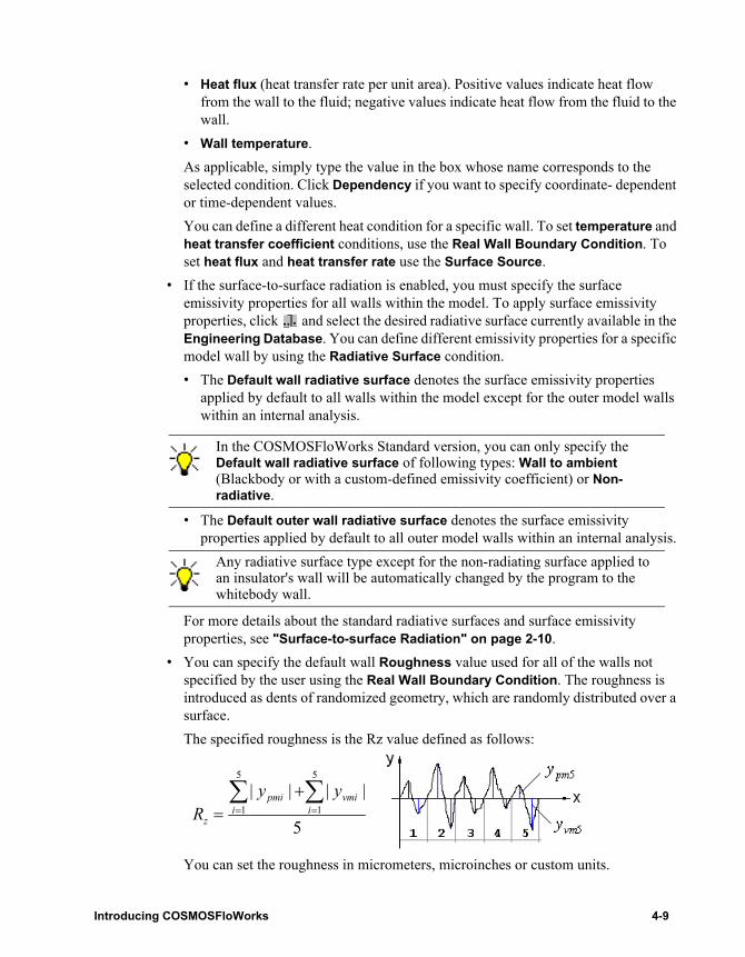
• Heat flux (heat transfer rate per unit area). Positive values indicate heat flow from the wall to the fluid; negative values indicate heat flow from the fluid to the wall.
• Wall temperature.As applicable, simply type the value in the box whose name corresponds to the selected condition. Click Dependency if you want to specify coordinate- dependent or time-dependent values.You can define a different heat condition for a specific wall. To set temperature and heat transfer coefficient conditions, use the Real Wall Boundary Condition. To set heat flux and heat transfer rate use the Surface Source.
• If the surface-to-surface radiation is enabled, you must specify the surface emissivity properties for all walls within the model. To apply surface emissivity properties, click and select the desired radiative surface currently available in the Engineering Database. You can define different emissivity properties for a specific model wall by using the Radiative Surface condition.• The Default wall radiative surface denotes the surface emissivity properties
applied by default to all walls within the model except for the outer model walls within an internal analysis.
• The Default outer wall radiative surface denotes the surface emissivity properties applied by default to all outer model walls within an internal analysis.
For more details about the standard radiative surfaces and surface emissivity properties, see "Surface-to-surface Radiation" on page 2-10.
• You can specify the default wall Roughness value used for all of the walls not specified by the user using the Real Wall Boundary Condition. The roughness is introduced as dents of randomized geometry, which are randomly distributed over a surface.The specified roughness is the Rz value defined as follows:
You can set the roughness in micrometers, microinches or custom units.
In the COSMOSFloWorks Standard version, you can only specify the Default wall radiative surface of following types: Wall to ambient (Blackbody or with a custom-defined emissivity coefficient) or Non-radiative.
Any radiative surface type except for the non-radiating surface applied to an insulator's wall will be automatically changed by the program to the whitebody wall.
5
||||5
1
5
1∑ ∑
= =
+= i i
vmipmi
z
yyR
Introducing COSMOSFloWorks 4-9

Chapter 4 Wizard
• Slip condition. In case of an analysis involving a non-Newtonian liquid, you can specify a Navier slip condition for all model walls. To apply the slip condition, select the checkbox in the Value cell at the right of the Slip effect parameter. You must specify values of C1 and C2 constants as well as the Yield stress. The Navier slip condition obeys the following law for the liquid's slip velocity at the wall:
,where τ - the shear stress obtained from the calculation, τ0,Gl - the yield shear stress specified by the user (Yield stress), VGl - the slip velocity at wall, C1 and C2 - constants specified by the user.
2 Click Next or click a button on the Navigator pane to switch to the corresponding dialog box of the Wizard.
After the project is created, you can change the Default wall conditions under Wall conditions in the General Settings dialog box.
See also "Heat Conduction in Solids" on page 2-2, "Boundary Conditions – Basic Information" on page 3-5.
Initial and Ambient Conditions
Specifying Initial (for an Internal analysis) or Initial and Ambient (for an External analysis) Conditions means specifying values of Thermodynamic parameters, Velocity parameters, Turbulence parameters, Concentration (for more than one fluid) and Solid parameters (to solve “Heat conduction in solids”).
• If you want to solve a steady Internal problem in a shorter time, we recommend that you use Initial conditions (initial values of the flow parameters) that are closer to the assumed solution than the default initial conditions.
• If you solve a steady External problem, specifying Ambient conditions means specifying initial conditions within the Computational Domain and boundary conditions at the Computational Domain boundaries. The specified thermodynamic and velocity parameters are considered as parameters of the undisturbed external flow and used to define the initial flow state.
• If you solve a time-dependent (transient) problem, you must specify initial values of the flow parameters exactly, with the exception of unsteady problems, which have a steady periodic solution (e.g. in the case of periodic boundary conditions) and can be obtained from arbitrary initial conditions, but additional time will be required to eliminate the initial conditions’ influence.
• You can specify initial conditions as constants or coordinate-dependent values. You can also apply results from other calculations as the project’s initial conditions.
4-10
• After passing the Wizard, you can replace these initial conditions by specifying other initial conditions in the General Settings dialog box and/or, in a local region (see "Creating an Initial Condition" on page 19-1).
Double-click a Value cell to edit the cell contents or select the appropriate parameter type. If you want to specify a coordinate-dependent or time-dependent value, click Dependency after clicking the corresponding Value box.
To specify initial and ambient conditions:
1 Under Parameter Definition select whether you want to manually specify initial (ambient) conditions or apply another project’s results as initial (ambient) conditions for the current project:
• Select User Defined for manual specification.• Select Transferred for using results from another calculation. See "Select
Results to Transfer" on page 4-17.To use the previous project calculation results as initial (ambient) conditions, use the Take previous results option. See "Running the Calculation" on page 24-1 for details.
2 Under Thermodynamic parameters select a combination of independent flow parameters (static pressure, static temperature, static density) and type the values in the corresponding boxes. For liquids the only available thermodynamic parameters are pressure and temperature.If you enable a rotating reference frame, you can select the Pressure potential check box. When the Pressure potential check box is selected, the specified initial static pressure is assumed to be relative to the rotating frame pressure (Pr) and the absolute pressure is determined by the density, angular velocity and the radius:
.When the Pressure potential box is unchecked, the specified initial static pressure is assumed to be a pressure in terms of the absolute frame of reference (Pabs), i.e. observable by the stationary analyst.If gravitation effects are considered, you can select the Pressure potential check box. When the Pressure potential check box is selected, the specified initial static pressure is assumed to be piezometric pressure (or potential) and the absolute pressure (Pabs) is determined by the reference density, gravitational acceleration vector and the position vector:
.When the Pressure potential box is unchecked, the specified initial static pressure is assumed to be an absolute pressure, and the corresponding piezometric pressure is respectively calculated.
3 Under Velocity parameters specify the X, Y and Z components of the velocity vector with respect to the Global Coordinate System. For gases you can specify the Mach
2 212specified r absP P P rρω= = − ⋅
( )specified piezo abs x y zP P P g x g y g zρ= = − + +
Introducing COSMOSFloWorks 4-11
Chapter 4 Wizard
number instead of the absolute velocity. When the Relative to rotating frame check box is selected, the specified velocity (Mach number) is assumed to be relative to the rotating reference frame (Vr):
.Clear this check box to specify velocity (Mach number) relative to the absolute (non-rotating) frame of reference (Vabs).
4 Under Turbulence parameters (if Laminar Only flow is not considered) you can adjust the default turbulence parameters if you are fully confident in your turbulent values. The default turbulence parameters are used as initial conditions (or ambient conditions for external analyses) in the computational domain and as a default inlet boundary condition in Boundary Conditions and Fans. You can set either turbulent Intensity and turbulent Length or turbulent Energy and turbulent Dissipation.
5 If the number of fluids selected as default fluids is greater than one, then under Concentration, specify the relative concentrations of the project’s default fluids either by Mass or by Volume. By default, COSMOSFloWorks uses equal concentrations for all fluids. COSMOSFloWorks uses the specified concentrations as initial conditions (or ambient conditions for external analyses) for the entire computational domain and as a default inlet boundary condition in Boundary Conditions and Fans.TIP: If you have several fluids piped into a volume, you can decrease the total calculation time by specifying the initial fluid concentrations within a pipe equal to the concentrations at the pipe’s inlet. To do this, replace a pipe fluid volume (the void) with a solid part, disable this part in the Component Control dialog box, and using the Local Initial Condition dialog box specify the appropriate initial fluid concentrations for the fluid region represented by this part.
6 In case of conjugate heat transfer problem, under Solid Parameters specify the Initial solid temperature assigned by default to all model components. This temperature is needed to start the calculation when solving a steady-state problem or to define the initial state when solving a time-dependent problem. However, you can specify a different initial solid temperature to a particular model component by using the Local Initial Condition dialog box.
7 Click Next or click a button on the Navigator pane to switch to the corresponding dialog box of the Wizard.
After the project is created, you can change the Initial and/or Ambient conditions under Initial (for an Internal analysis) or Initial and ambient conditions (for an External analysis) in the General Settings dialog box.
r absV V rω= − ×
4-12

Results and Geometry Resolution
Results and Geometry Resolution in the form described below is specified in the Wizard only. After finishing the Wizard, the Result resolution is virtually split into Level of initial mesh on the Automatic Settings tab of the Initial Mesh dialog box, governing the initial mesh only, and Results resolution level in the Calculation Control Options dialog box, governing finishing the calculation and refining computational mesh during calculation. As for the Geometry resolution options, influencing the initial mesh also, they can be changed on the Automatic Settings tab of the Initial Mesh dialog box, and/or their effects can be corrected in the Local Initial Mesh dialog box.
Result resolution governs the solution accuracy through mesh settings and conditions of finishing the calculation that can be interpreted as resolution of calculation results. You specify result resolution in accordance with the desired solution accuracy, available CPU time and computer memory. Because this setting has an influence on the number of generated mesh cells, a more accurate solution requires longer CPU time and more computer memory.
To specify result resolution:
1 Using the slider, you can select one of the eight resolution levels. The first level will give the fastest results but the level of accuracy may be poor. The eighth level will give the most accurate results but may take a long time to converge. Increase result resolution level if you want to improve the quality of the results.The resolution level that will return stable results depends on the task. For the majority of tasks you can achieve stable results starting from level three. However, some types of tasks require increasing the result resolution level (e.g. external flows with separation from smooth surfaces).
2 Click Finish to close the Wizard and create an COSMOSFloWorks project or specify the geometry resolution parameters as described below.
Geometry resolution. Allows you to specify the Minimum gap size and Minimum wall thickness to discern diminutive geometry that is not automatically recognized by COSMOSFloWorks. These settings have an influence on a characteristic cell’s size and together with Result Resolution govern the total number of cells generated in the computational mesh.
COSMOSFloWorks calculates the default minimum gap size and minimum wall thickness using information about the overall model dimensions, the Computational Domain, and faces on which you specify Conditions and Goals. However, this information may be insufficient to recognize relatively small gaps and thin model walls. This may cause inaccurate results. In these cases, the Minimum gap size and Minimum wall thickness must be specified manually.
Introducing COSMOSFloWorks 4-13

Chapter 4 Wizard
Prior to starting the calculation, we recommend that you check the geometry resolution to ensure that small features will be recognized. Use FloWorks, Project, Summary to observe the Minimum gap size and the Minimum wall thickness. If you set boundary conditions, surface goals, or modify the model or computational domain, these characteristic sizes may change. Click FloWorks, Project, Rebuild to update the minimum gap size and minimum wall thickness.
To specify geometry resolution:
1 Specify the minimum gap size and the minimum wall thickness:• Minimum gap size. The automatically generated minimum gap size depends on
the model size, computational domain, volume sources, initial conditions, and boundary conditions. If the model has a gap that is smaller than the Minimum gap size, then the gap will not be considered during the calculation (i.e., fluid will not pass through the gap). To specify a minimum gap size manually, select Manual specification of the minimum gap size and type the value in the Minimum gap size box.You can link the minimum gap size value to a feature or reference dimension so that the minimum gap size value will be equal to the dimension. Changing the dimension value causes the minimum gap size value to change. To link the minimum gap size value, click the Minimum gap size refers to the feature dimension check box and select the dimension in the graphics area. To display all possible dimensions, right-click the Annotations item in the FeatureManager tree and select Show Feature dimensions and Show Reference Dimensions.
• Minimum wall thickness. The automatically generated minimum wall thickness value depends on the model size, computational domain, volume sources, initial conditions, surface sources and surface goals. The Minimum wall thickness does not influence the meshing if it is equal to or greater than the Minimum gap size (see "Automatic Settings for Initial Mesh" on page 21-1). If the model has walls or solid protrusions whose thickness is less than the Minimum wall thickness and Minimum gap size, then the solid walls with both sides contacting the fluid will not be resolved properly during the calculation (i.e., the solid will be replaced with fluid). To specify a minimum wall thickness manually, select Manual specification of the minimum wall thickness and type the value in the Minimum wall thickness box.You can link the minimum wall thickness value to a feature or reference dimension so that the minimum wall thickness value will be equal to the dimension. Changing the dimension value causes the minimum wall thickness value to change. To link the minimum wall thickness value, click the Minimum wall thickness refers to the feature dimension check box and select the dimension in the graphics area. To display all possible dimensions, right-click the Annotations item in the FeatureManager tree and select Show Feature dimensions and Show Reference Dimensions.
4-14

The manually specified values are retained if you modify the model or COSMOSFloWorks project.
If you specify very small values of these reference sizes and a high result resolution, the number of mesh cells will dramatically increase, resulting in increases in memory requirements and CPU time.
2 You can also select the Advanced narrow channel refinement option checkbox. When checked, a finer narrow channel refinement strategy is enabled which ensures that narrow channel flow passages will be resolved by a sufficient number of cells to predict the flow and heat transfer phenomena with higher accuracy. The consequence may be a significant increase of the number of cells (up to one or more orders of magnitude).
3 Click Finish to close the Wizard and create an COSMOSFloWorks project or click a button on the Navigator pane to switch to the corresponding dialog box of the Wizard.
Rotation
If you deal with rotating equipment you can model the flow in the coordinate system rotating with the rotating equipment.
To enable rotation:
1 In the Analysis Type dialog box select the Rotation check box.2 Select the Type of rotation:
• Local region(s). If you select Local region(s) you can specify the local rotating reference frame(s). This allows you to analyze the fluid flow through rotating components of the model. In order to specify the local Rotating region you need to create a component representing it. The fluid flow within the rotating region is calculated in the rotating region’s local reference frame. Flow field parameters are transferred from adjacent flow regions to the rotating region’s boundary as boundary conditions. The flow field must be axially symmetric at the rotating region’s boundary. See "Rotating Regions" on page 9-1.
• Global rotating. If you select Global rotating it is assumed by default that all model walls rotate at the speed of the rotating reference frame. At that, the corresponding Coriolis and centrifugal forces are taking into account.You can specify a stator (non-rotating in the absolute, inertial reference frame) face that must be symmetric with respect to the rotation axis. To specify a stator face, use the Stator moving wall boundary condition. By default when you enable a rotating
In case of internal analyses, boundaries between internal flow and ambient space are always resolved properly because COSMOSFloWorks distinguishes the internal flow volume and ambient space. If your model does not contain walls with both sides contacting the fluid and it does not contain thin features protruding into the fluid, then the Minimum wall thickness value should not be changed.
Introducing COSMOSFloWorks 4-15

Chapter 4 Wizard
reference frame, velocity (Vr) and pressure (Pr) values are specified relative to the rotating reference frame as follows:
Here, Vabs and Pabs are the velocity and pressure in the absolute or stationary reference frame correspondingly, w is the angular velocity, r is the density and r is the distance from the axis of rotation. You can also specify velocity and pressure values in the absolute reference frame (i.e. Vabs and Pabs) if you clear the “Relative to rotating frame” option for velocity specification and the “Pressure potential” for pressure specification.
3 If you have selected the Global rotation option, click and in the Rotation Axis dialog box specify the rotational axis as either a reference axis or an axis of reference coordinate system:
• In the FeatureManager tree, select a reference Axis. To create an axis, go to Insert, Reference Geometry, Axis. When you select a reference axis check to see that its direction conforms to the angular velocity value: positive angular velocity value denotes angular velocity vector codirectional with the axis direction. The direction of the axis is indicated by the axis’ name that is shown near the axis origin.
• In the FeatureManager tree, select a reference Coordinate system (or keep the default Global Coordinate System), then in the Rotation axis, select an axis of this coordinate system you want to be a rotation axis. To create a reference coordinate system go to Insert, Reference Geometry, Coordinate System. The positive angular velocity value denotes angular velocity vector codirectional with the axis direction.
4 If you have selected the Global rotation option, specify an Angular Velocity value (ω) which obeys the right-handle rule.
5 If you are finished specifying parameters in the Analysis Type dialog box click Next or click a button on the Navigator pane to switch to the corresponding dialog box of the Wizard.
Rotation Axis
Allows you to specify the rotational axis of the global rotating frame of reference:
To specify the rotation axis:
1 Select either a reference axis or an axis of reference coordinate system:
The displayed arrows always show direction corresponding to the positive angular velocity value.
r absV V rω= − ×
2 212r absP P rρω= − ⋅
4-16
• In the FeatureManager tree, select a reference Axis. To create an axis, go to Insert, Reference Geometry, Axis. When you select a reference axis check to see that its direction conforms to the angular velocity value: positive angular velocity value denotes angular velocity vector codirectional with the axis direction. The direction of the axis is indicated by the axis’ name that is shown near the axis origin.
• In the FeatureManager tree, select a reference Coordinate system (or keep the default Global Coordinate System), then in the Rotation axis, select an axis of this coordinate system you want to be a rotation axis. To create a reference coordinate system go to Insert, Reference Geometry, Coordinate System. The positive angular velocity value denotes angular velocity vector codirectional with the axis direction.
2 Click OK.
Select Results to Transfer
Allows you to select a COSMOSFloWorks project or results file (*.fld), whose results will be applied as initial conditions for the current project. If the parameter values to be applied cannot be applied to the current project due to differences in the projects (e.g., differences in computational domains or fluid and solid regions, so that a parameter in the project of reference is not defined in the current project) then the default values (specified under the Thermodynamic Parameters, Velocity Parameters, Turbulence Parameters and other items) will be used in the current project.
To select results to transfer:
1 Select the method in which the results are taken:• Select COSMOSFloWorks project, if you want to take the results of a currently
opened model’s project. This is the easiest way to take results obtained earlier in the project of the current model. If you want to take results obtained in another model, you need to open this model first or use the COSMOSFloWorks results (*.fld) file option.
• Select Results (*.fld) file if you want to take the results from a results (*.fld) file of any available COSMOSFloWorks project.
2 Click Browse to select either the desired COSMOSFloWorks project or the desired COSMOSFloWorks results (*.fld) file. As a result, the project (or file) name appears in the Selected COSMOSFloWorks project or results (*.fld) file box.
The displayed arrows always show direction corresponding to the positive angular velocity value.
COSMOSFloWorks stores results in the <ProjectNumber>.fld file. This file is stored in the project folder accessible by clicking FloWorks, Project, Open Project Directory. The r_000000.fld file contains results obtained for the zero iteration, i.e. initial computational mesh and initial parameters distribution.
Introducing COSMOSFloWorks 4-17

Chapter 4 Wizard
3 Click OK.
4-18

5 Working with Project
New Project
Creates a COSMOSFloWorks project based on a standard or user defined Template, instead of using the Wizard. In General Settings, Calculation Control Options, Initial Mesh, Units you specify information required for the new project. Creating similar projects this way is convenient, but remember that Fluid Subdomains, Rotating Regions, Boundary Conditions, Transferred Boundary Conditions, Initial Conditions, Porous Media, Heat Sources, Fans, Contact Resistances, Heat Sink Simulations, Surface Goals, and Volume Goals, and Equation Goals data are not saved in Templates.
COSMOSFloWorks uses SolidWorks configurations as a geometry basis for projects. You can create a COSMOSFloWorks project in one of the following ways:
• Create a new project and configuration. Using this method, you define a new configuration for the new COSMOSFloWorks project that is based on an existing configuration.
• Use current configuration. This method attaches a new COSMOSFloWorks project to the currently active configuration. The project name is the same as the current configuration.
To create a new project and configuration:
1 Click FloWorks, Project, New.2 Click Create new.3 Enter a Configuration name for your COSMOSFloWorks project.4 From the Basic configuration list select the desired SolidWorks configuration with
the geometry you want to use as a basis for the analysis.
Introducing COSMOSFloWorks 5-1

Chapter 5 Working with Project
5 Select the desired template from the List of templates. If there were no extra templates created, only the New Project default template is available. See "Template" on page 5-3.
6 Click OK.
To add a new project to the current configuration:
1 Click FloWorks, Project, New.2 Click Use current.3 Select the desired template from the List of templates. If there were no extra templates
created, only the New Project default template is available. See "Template" on page 5-3.
4 Click OK.If the current configuration already contains a project, a warning message appears.The message asks if you want to replace the existing project:
• If you click Yes, the existing project is replaced by the new one and all data associated with the old project will be lost.
• If you click No, the new project is not created.To avoid the warning message you should Clear Configuration first.
See also "COSMOSFloWorks Project" on page 1-4.
Clone Project
Allows you to create an exact copy of the current project. You can either use an existing configuration or copy it to a new configuration for the project you clone. This may be useful if you need to compare variants of a model with a few changes such as small discrepancies in geometry, different boundary conditions or fluids.
The project settings such as General Settings, Conditions, Goals, Units and results features are copied to the new project. If results are available, you can also copy them. In this case, the current and cloned project are identical.
To clone a project and create a new configuration:
1 Click FloWorks, Project, Clone Project.2 Click Create new.3 Enter a Configuration name for your project.
While modifying a current configuration, remember, that adding or deleting SolidWorks features may have an influence on the other model configurations depending on the properties of each configuration. Feature changes may cause errors in COSMOSFloWorks projects attached to other configurations.
5-2
4 Select Copy results, if desired.You copy the existing results for the possibility to use them as global initial conditions for the cloned project.
5 Click OK.
To clone a project and assign it an existing configuration:
1 Click FloWorks, Project, Clone Project.2 Click Add to existing.3 From the Existing configuration list select the desired configuration with the
geometry you want to use as a basis for the analysis.4 Select Copy results, if desired. You copy the existing results for the possibility to use
them as global initial conditions for the cloned project.5 Click OK.
If the current configuration already contains a project, a warning message appears.
The message asks if you want to replace the existing project:
• Click Yes, to replace the existing project by the cloned project. In this case all data associated with the old project will be lost.
• Click No to choose another configuration for the project you clone.
To avoid the warning message you should Clear Configuration first. See "Clear Configuration" on page 5-5.
Template
Template contains all general project settings that can be used as a basis for a new project. These settings (problem type and physical features, fluids, solids, initial and ambient flow parameters, wall condition, geometry and result resolution, unit settings) can be specified under General Settings, Calculation Control Options, Initial Mesh and Units.
Notice that Fluid Subdomains, Rotating Regions, Boundary Conditions, Porous Media, Fans, Local Initial Conditions, Solid Materials, Heat Sources, Radiative Surfaces, Contact Resistances, Heat Sink Simulations, Surface Goals, Volume Goals, and Equation Goals, as well as results are not stored in the template. To clone (copy) a project, see "Clone Project" on page 5-2.
Initially, only the New Project default template is available.
To create a new template:
1 Under the General Settings, Initial Mesh, Calculation Control Options, and Unit dialog boxes, specify data you want to store in the template.
2 Click FloWorks, Project, Create Template.3 Enter a descriptive Template name. 4 Click Save.
Introducing COSMOSFloWorks 5-3

Chapter 5 Working with Project
After the template is created, it is available in the list of templates, which you can use as a basis for a new project.
COSMOSFloWorks Default Template
The default “New project” template has the following settings:
Analysis Type InternalPhysical Features
• Heat conduction in solids OFF (no solids defined)• Heat conduction in solids only OFF• Radiation OFF• Time dependent OFF• Gravity OFF• Rotation OFF
Default Fluid
• Default fluid type Liquid• Project fluids Water• High Mach number flow OFF• Flow type Laminar and Turbulent
Default wall thermal condition Adiabatic wall
Roughness 0 micrometersThermodynamic parameters
• Pressure 101325 Pa• Temperature 293.2 K
Velocity parameters 0 m/sTurbulence Parameters
• Turbulence intensity 2%• Turbulence length <Dependent on the model size>
Level of initial mesh Level 3
Geometry Resolution <Dependent on the model size>
Advanced narrow channel refinement OFF
5-4
Clear Configuration
Allows you to disconnect the current COSMOSFloWorks project with the active SolidWorks configuration and delete the project. When clearing a configuration, you can keep all project files such as COSMOSFloWorks files, Excel and Word documents, images and AVI files.
Once you clear a configuration, you will not be able to restore the project.
To clear a configuration:
1 Click FloWorks, Project, Clear Configuration.2 Click Yes to confirm that you want to delete the directory and all the project files
associated with the active configuration. Click No if you want to disconnect the project and leave all the project files. Click Cancel to abandon the operation.
Edit Comment
Allows you to edit project comments.
In addition to the project Summary, here you can enter information about specified boundary and initial conditions, fans, sources and goals.
Summary
Presents general information about the project:
• Project name. The name of the SolidWorks configuration to which the project is connected.
• Project output directory. The default directory for storing project files, output images, reports and Excel documents.
• System of units.• Analysis type.• Results resolution level.• Geometry resolution.• Default fluid type, number of fluids, fluids.• Physical features.• Default thermal wall condition or Number of solid substances (if heat conduction in
solids is enabled).• Default roughness value.• Initial conditions (or Initial and ambient conditions, for External flow problems).• Mass or volume substance fractions (for multiple fluids).
Introducing COSMOSFloWorks 5-5

Chapter 5 Working with Project
• Default solid substance and initial solid temperature (if heat conduction in solids is enabled).
• Computational domain size and type of boundary condition specified at the computational domain boundary.
• List of parts and subassemblies disabled in the Component Control dialog box.• The specified boundary conditions and sources.
Rebuild Project
If you have modified the SolidWorks model, click FloWorks, Project, Rebuild to update the project settings.
COSMOSFloWorks detects when the project requires a rebuild and asks you for the rebuild. You can switch off this detection by clearing the Automatic Rebuild option accessible under FloWorks, Project menu.
You must also rebuild the project after you rectify any Rebuild Error encountered by COSMOSFloWorks.
Copy Features among Projects
Allows you to copy project’s Input Data and Results features from the active project to other projects within the same model.
To copy features to other projects:
1 Click FloWorks, Tools, Copy Features.- or -In the COSMOSFloWorks analysis tree, right-click the feature you want to copy and select Copy to Project.
2 In the Target projects list select projects you want to copy the selected features to.3 Select features to copy. You can select more than one feature by holding down the Ctrl
key while selecting the features in the analysis tree. To remove a feature from the list, select the feature and click Remove.
4 Click OK .
Parameter Editor
Allows you to edit parameter values of different input data features (boundary conditions, initial conditions, fans, etc.) from different projects using the same dialog box. You can edit parameter values of several features simultaneously, if the parameters are common for the selected features.
5-6

To edit parameter values:
1 Click FloWorks, Tools, Parameter Editor.
2 In the list of Features, select features whose parameters you want to edit. If you want to select several features, hold down the Ctrl key while selecting. Common parameters for the selected features appear in the Parameters list.If a parameter value is not the same for all of the selected features, you will see <Different> in the Value cell for this parameter. If a parameter has a Boolean value (check box), then <Different> is added to the parameter’s name.
3 Double-click the Value cell in the list of Parameters to edit the parameter value.If you want to specify a coordinate-dependent or time-dependent value, click Dependency after clicking the corresponding Value box. See "Dependency" on page 22-1 for details.
4 Click OK to accept changes and close the dialog box or click Apply to update and continue to make changes.
Component Control
Allows you to control the component state. Components (parts or subassemblies in assemblies, as well as bodies in multibody parts) can be either disabled or enabled. This setting affects neither your model nor the configuration. COSMOSFloWorks treats disabled components as fluid, so you can specify initial conditions that are different from the defaults, as well as specify local regions of rotation, volume sources and volume goals, etc.
You can disable components to:
• Specify a Rotating Region.• Specify Local Initial Condition or Volume Source, or Volume Goal in fluid.• Specify a Porous Medium.• Exclude unused components from the analysis if suppressing them causes invalid
geometry (note that suppressing is the preferred method for excluding components not needed for the fluid analysis).
• Specify Local Initial Mesh.
To disable components:
1 Click FloWorks, Component Control.– or –In the COSMOSFloWorks analysis tree double-click the Component Control icon, or right-click it and select Run Component Control.
2 In the Components tree, select parts or subassemblies to disable. You can select a group of components by holding Ctrl while selecting them.
Introducing COSMOSFloWorks 5-7

Chapter 5 Working with Project
3 Click Disable.– or –Click Disable All if you want all components to be treated as a fluid.
4 Click OK.
To hide the disabled components in the graphics area:
Right-click the Component Control icon in the COSMOSFloWorks analysis tree and select Hide Unused Components.
Specifying Components Transparent for the Heat Radiation
If you consider radiative heat transfer you may deal with bodies which practically do not absorb neither emit thermal radiation so their influence on the radiative heat balance is negligible. Such bodies can be considered as bodies transparent for the radiative heat transfer.
Making a component transparent for the radiative heat transfer means that this component (part or subassembly) does not participate in the radiation heat transfer (i.e. neither emits nor absorbs heat radiation) and exchanges the heat by convection and conduction only.
Because transparent bodies do not participate in radiation, it is not allowed to specify radiative properties (as radiative surface condition) on their surfaces.
To make bodies transparent for radiative heat transfer:
1 Click FloWorks, Radiation Transparent Bodies.2 In the Components tree, select parts or subassemblies you want to make transparent
for radiation. You can select a group of components by holding Ctrl while selecting them.
3 Click Transparent. Click All Transparent if you want all components to be transparent for heat radiation.
4 Click OK.
5-8

Insert small solid brick into cube and make the brick transparent for the heat radiation (before inserting the brick, create an orifice in the cube's wall with dimensions corresponding to the size of the brick).
The solid brick prevents the external fluid from flowing into the cub but allows the ambient radiation to heat the inner cube’s walls.
Excluding Unused Components from the Analysis
In the analysis of an assembly there may be many parts or subassemblies that are not necessary for the analysis (for example, a bolted connection in a valve analysis). To save computer resources and increase the calculation speed, you can exclude these components from the analysis before the calculation starts.
You can exclude unused components by suppressing single parts or subassemblies within SolidWorks. In this case all corresponding mates are also suppressed. This may cause invalid geometry.
Alternatively, to retain all mating relations you can use the COSMOSFloWorks Component Control to disable a component (a part or subassembly in assemblies, as well as a body in multibody parts). Components disabled in the Component Control dialog box are treated as fluid. This allows you to exclude components from the analysis without suppressing them. Additionally, the disable function allows you to specify Rotating Regions, Initial Conditions, Volume Sources, Volume Goals or Porous Media in the component that is now treated as fluid.
Suppressing components is the preferred method since both SolidWorks and COSMOSFloWorks will effectively remove the components from the analysis.
Introducing COSMOSFloWorks 5-9

Chapter 5 Working with Project
Working with Lightweight PartsBecause a lightweight part does not store all data associated with the part, COSMOSFloWorks does not support the lightweight mode, thus resolving lightweight parts on opening the model. If after resolving lightweight parts some data is still missing, you need to rebuild the project. To avoid such problems, do not use lightweight parts while working with COSMOSFloWorks and check to see that the Automatically load parts lightweight option is disabled under both the Performance and Large Assembly Mode pages of the System Options dialog box, accessible by clicking Tools, Options.
5-10

6 General Settings
General Settings – Overview
General Settings together with the New Project, Initial Mesh, Calculation Control Options and Unit System is an alternative way to create a COSMOSFloWorks project (as opposed to using the Wizard).
The General Settings approach is essentially the Wizard with some minor but important differences. In particular, General Settings allows the use of a Template created from a previous COSMOSFloWorks project (see "New Project" on page 5-1), greatly minimizing data input. You modify the project created with the template in accordance with the new project requirements.
Additionally, you can apply General Settings to correct the settings made in the Wizard. The General Settings always presents the current state of the project parameters.
Remember that the Computational Domain size saved in the template may become inadequate after some changes performed in General Settings. For example:
• If you change the ambient velocity vector (in magnitude and/or in direction), or • If you switch from one analysis type to another (external or internal).
To avoid these inadequacies, we recommend that you reset the Computational Domain after performing General Settings: Right-click Computational Domain in the COSMOSFloWorks analysis tree, select Edit Definition and click Reset on the Size tab.
To perform general settings:
1 Click FloWorks, General Settings. 2 Click a button on the Navigator pane to switch to the corresponding dialog box of the
General Settings. The following dialog boxes can be available depending on the analysis type and selected physical features:• Analysis type (analysis type and physical features)
Introducing COSMOSFloWorks 6-1

Chapter 6 General Settings
• Fluids and fluid type (gas, liquid, non-Newtonian liquid, compressible liquid or steam)
• Solids (if Heat conduction in solids is enabled)• Wall conditions:
• Default outer wall thermal condition (if Heat conduction in solids is enabled)• Default wall thermal condition (if Heat conduction in solids is disabled)• Default wall radiative surface (if Radiation is enabled)• Default outer wall radiative surface (if Radiation is enabled)• Roughness • Slip condition (if the Non-Newtonian liquid is selected as the Default fluid
type)• Initial (Initial and ambient conditions for External analysis) Conditions:
• Thermodynamic parameters • Velocity Parameters
• Turbulence parameters • Concentrations (if several fluids have been specified)• Solid parameters (if Heat conduction in solids is enabled)
Analysis Type
Allows you to define an appropriate analysis type and select specific physical feature options for the problem you intend to solve with COSMOSFloWorks.
To specify an analysis type and physical feature options:
1 Under Analysis type select either Internal or External type of the flow analysis: • Internal flow analysis concerns flows bounded by outer solid surfaces, e.g.,
flows inside pipes, tanks, HVAC systems, etc. To perform an Internal flow analysis, the SolidWorks model must be fully closed (see "How It Works" on page 1-1). To make sure the model is closed use Check Geometry.
• External flow analysis concerns flows not bounded by outer solid surfaces, but only by the Computation Domain boundaries. In this case the solid model is fully surrounded by the flow, e.g., flows over aircrafts, automobiles, buildings, etc. If you want to analyze both internal and external flows simultaneously, e.g. flows over and through a building, the analysis is treated as an External analysis in COSMOSFloWorks.
6-2
2 For models that have internal spaces not involved in the flow analysis, you can use two additional options for reducing the required system resources under Consider closed cavities:
• Exclude internal spaces. Allows you to disregard closed internal spaces in External flow analyses.
• Exclude cavities without flow conditions. In both Internal and External flow analyses select this option if you want to exclude closed internal spaces with no Boundary Conditions or Fans specified on their surfaces.
Both procedures do not affect the SolidWorks model but allow you to avoid unnecessary mesh refinements and flow calculations in non-analyzed model regions. If you select these options the corresponding spaces and cavities are filled with solid.
3 Specify the following Physical features you want to take into account in the flow analysis. Double-click a Value cell to edit the cell contents or select the appropriate feature. If you want to specify a coordinate-dependent or time-dependent value, click Dependency after clicking the corresponding Value cell.
• Select the Heat conduction in solids check box if you want to analyze heat transfer in solid parts in contact with the fluid (conjugate heat transfer problem). See also "Heat Conduction in Solids" on page 2-2.
• Select the Heat conduction in solids only check box if no fluid exists in your heat transfer analysis.
• Select the Radiation check box if you want to enable surface-to-surface radiation in conjugate heat transfer analysis. See "Surface-to-surface Radiation" on page 2-10. • You can select the Environment radiation option. The Environment
radiation can be specified for both external and internal analyses. It denotes that the computational domain’s far-field boundaries radiates heat (Q) into the computational domain using the Emissivity coefficient (ε = 1, specified in the Engineering Database under the Radiative Surface, FW Defined, Blackbody opening/outer boundary item) and the specified Environment temperature as shown below:Q = ε σT4.
• Select the Solar radiation check box to enable directional radiation from ambient space and specify the directional vector (using the X, Y, Z components of the direction vector) and the Intensity.
• Select the Time dependent check box if your problem is transient (i.e., unsteady). You can modify the settings for time-dependent analysis in the Calculation Control Options dialog box.
• Select the Gravity check box if you need to take gravitational effects into account, and specify the acceleration due to gravity X, Y, and Z components in
Excluding internal spaces or cavities may cause wrong results if you analyze heat exchange between solid parts and fluid volumes.
Introducing COSMOSFloWorks 6-3

Chapter 6 General Settings
the Global Coordinate System. This option, for example, should be used for natural (free) convection heat transfer problems.For time-dependent analyses, you can specify the gravitational acceleration vector dependent on time by clicking Dependency. If liquids are used, check to see that the densities specified in Engineering Database are dependent on the fluid temperature. If gases are used, you cannot use Gravity when the High Mach number flow option is enabled.
• Select the Rotation check box if you want to specify either Local region(s) of rotation or the Global rotating reference frame. For a Global rotating reference frame you need to specify the Reference axis and the Angular velocity. Please note that the Radiation and Time dependent options will be unavailable if you select Local region(s) of rotation. Also, you should not use Local region(s) of rotation if you want to analyze high Mach number flows. See "Rotation" on page 6-12.
4 Specify Reference axis of the global coordinate system (X, Y or Z). This axis is used in the Dependency dialog box for specifying data as tabular or formula dependencies on the radial (r) coordinate reckoned in a cylindrical coordinate system from the reference axis.
5 Click Apply to update and proceed with settings- or - Click OK to apply the changes and exit the dialog.
Fluids
Allows you to change the fluid type as well as add, remove or replace the fluid substances.
When you replace fluids, all previous fluid references are assigned to a new fluid. This function is convenient if you have more than one fluid. For example, while creating a Boundary Condition, you define a mixture that flows into the opening by adjusting the concentrations. Then if you want to analyze a different mixture component, you simply Replace one of the fluid substances. Otherwise, if you Add a fluid you must readjust the concentration.
COSMOSFloWorks allows you to analyze the flow of up to ten fluids of different types (Liquids, Gases/Steam, Non-Newtonian Liquids and Compressible Liquids) in the same project. Fluids mixing can be analyzed as well (except for Compressible Liquids), but mixing fluids must be of the same type. In the Fluids dialog box you can specify the default fluids and default fluid type to be assigned for all fluid regions. You can specify different fluid types for specific fluid regions using the Fluid Subdomain feature. Fluid regions with different types of fluids must be separated from each other by solid region(s).
6-4

COSMOSFloWorks is capable of calculating only laminar flow of inelastic non-Newtonian liquids or compressible liquids, thus if you want to deal with non-Newtonian liquids, you have to select the Laminar Only flow type under the Problem type item to consider the entire flow as laminar.
To specify the project fluids and default fluids:
1 In the Fluids list, click at the left of fluid type name to display the list of fluids of this type available in the Engineering Database. The fluid types are: Gases, Liquids (Newtonian viscous incompressible liquids), Non-Newtonian liquids, Compressible liquids and Steam. See also "Fluid Type and Compressibility" on page 2-4, "Water Vapor Condensation" on page 2-8, "Non-Newtonian Liquids" on page 2-8, "Compressible Liquids" on page 2-9.If you discover that the required fluid is not available, click New and add the new fluid to the Engineering Database.
2 Double-click the desired fluid in the Fluids list.– or –Select a fluid from the Fluids list and click Add.The Project fluids list displays fluids that are available for the current analysis. To remove a fluid from the analysis select it in the Project fluids list and click Remove.• If you have added fluids of different types to the Project fluids list, you must select
the Default fluid type. Only fluids of this type will be available to be assigned as default project fluids. The selected fluid type is assigned by default for all fluid regions in the analysis. You can specify another fluid type for a specific fluid region using the Fluid Subdomain feature.
• If you have added more than one fluid of the same type to the Project fluids list, you can select which of them will be assigned as default fluids for all fluid regions by selecting check boxes at the right of each fluid’s name. You can assign other fluids for a specific fluid region using the Fluid Subdomain feature; only fluids specified in the Project fluids list will be available for selection. Default fluids’ concentrations are specified in the Initial Conditions (Initial and Ambient Conditions for External analysis) dialog box of the General Settings and assumed equal by default.
3 Click Apply to update and proceed with settings.– or –Click OK to apply the changes and exit the dialog.
To change the default fluid type:
1 In the Project fluids list select the Default fluid type, which is assigned by default for all fluid regions in the analysis. Only fluids of this type will be available to be assigned as default project fluids. If the desired fluid type is not available for selection this means that no fluids of this type are in the Project fluids list. In this case you should add the required fluids of this type by selecting them in the Fluids list and clicking Add. See also "Fluid Type and Compressibility" on page 2-4.
Introducing COSMOSFloWorks 6-5

Chapter 6 General Settings
2 Specify the fluids to be assigned as default fluids for all fluid regions by selecting check boxes at the right of each fluid’s name. Default fluids’ concentrations are specified in the Initial Conditions (Initial and Ambient Conditions for External analysis) dialog box of the General Settings and assumed equal by default. You can assign other fluids for a specific fluid region using the Fluid Subdomain feature. If you have already specified one or more Fluid subdomains, their settings will be retained.
3 Depending on the Default fluid type, you can also specify the following Flow Characteristics: • Flow type. By default, the flow can be either laminar or turbulent or with transition
(depending on the flow characteristics). Under Flow type, you can consider the flow as laminar only in the entire Computational Domain by selecting Laminar Only, or turbulent only by selecting Turbulent Only correspondingly. If you have specified Non-Newtonian liquids or Compressible liquids as the project's fluid type, the Laminar Only flow type will be selected automatically to consider the flow in all fluid regions as laminar. You can specify another fluid type and, therefore, another flow type for a specific fluid region using the Fluid Subdomain feature. See also "Turbulence" on page 2-5.
• High Mach number flow. Select the High Mach number flow check box if you want to analyze high-velocity gas flows (flow Mach number is greater than about 3 for steady-state and 1 for transient analyses). The High mach number option is applied for the entire computational domain and cannot be changed for an individual fluid region. See also "Fluid Type and Compressibility" on page 2-4.
4 Click Apply to update and proceed- or -click OK to apply the changes and exit the dialog.
To replace one of the project fluid:
1 Under Fluids, select a fluid you want to add in the analysis.2 In the Project fluids list select a fluid you want to replace.3 Click Replace.4 Click Apply to update and proceed
- or -click OK to apply the changes and exit the dialog.
Solids
Allows you to specify the default solid material applied to all solid components in a conjugate heat transfer analysis.
This will reduce the amount of data entry required for models with many components. If you want to specify a different solid material for one or more components, you can define a Solid Material condition for these components.
6-6

If there is no appropriate solid listed in the Solids list, click New and define a new substance in the Engineering Database.
To specify the default solid material:
1 Select a solid material from the Solids list taken from the Engineering Database. Selected material appears in the Default solid box.
2 Click Apply to update and proceed with settings- or -Click OK to apply the changes and exit the dialog.
To replace the default solid material:
1 From the Solids list select a solid material with which you want to replace the current default solid material. Selected material appears in the Default solid box.
2 Click Apply to update and proceed with settings- or -Click OK to apply the changes and exit the dialog.
Default Wall Conditions
Allows you to specify the conditions applied to all model walls by default.
To specify default wall conditions:
1 Specify the Value of the wall condition Parameter. The following types of wall conditions are available depending on the analysis type and physical features specified in the Analysis Type dialog box of the General Settings:• Default outer wall thermal condition. In case of internal analysis with Heat
conduction in solids enabled, you must specify a thermal condition applied by default to all the outer model walls. This condition allows you to define the heat exchange between the external flow and the outer model walls for internal analysis.The following thermal conditions can be set on the outer model walls:• Adiabatic wall. This is a heat-insulated wall.• Heat transfer coefficient. The heat flow (Q) through the outer walls is denoted
by the user-defined Heat transfer coefficient (α), Temperature of external fluid (Tf), the calculated temperature of the outer wall (Ts) and the wall area (S): Q = α(Tf - Ts)S.
• Heat generation rate (total heat generation rate). Positive values indicate heat flow from the outer media to the solid; negative values indicate heat flow from the solid to the outer media.
• Surface heat generation rate (heat generation rate per unit area). Positive values indicate heat flow from the outer media to the solid; negative values indicate heat flow from the solid to the outer media.
• Wall temperature. Specifies the outer wall temperature.
Introducing COSMOSFloWorks 6-7

Chapter 6 General Settings
Click Dependency if you want to specify coordinate-dependent or time-dependent values.You can redefine the default heat condition for a specific outer wall: to specify the heat generation rate or surface heat generation rate conditions, use Surface Source; to specify the heat transfer coefficient use the Outer Wall boundary condition.
• Default wall thermal condition. If you do not intend to solve a conjugate heat transfer problem, you must specify one of the following heat wall conditions applied by default to all of the model walls contacting with the fluid:• Adiabatic wall. This is a heat-insulated wall. By default all walls are skin friction
surfaces. If you want the wall to be adiabatic and frictionless, you must create a boundary condition type of Ideal Wall on the appropriate faces.
• Heat transfer rate (total heat transfer rate). Positive values indicate heat flow from the wall to the fluid; negative values indicate heat flow from the fluid to the wall.
• Heat flux (heat transfer rate per unit area). Positive values indicate heat flow from the wall to the fluid; negative values indicate heat flow from the fluid to the wall.
• Wall temperature.As applicable, simply type the value in the box whose name corresponds to the selected condition. Click Dependency if you want to specify coordinate-dependent or time-dependent values.You can define a different heat condition for a specific wall. To set temperature and heat transfer coefficient conditions, use the Real Wall Boundary Condition. To set heat flux and heat transfer rate use the Surface Source.
• If the surface-to-surface radiation is enabled, you must specify the surface emissivity properties for all walls within the model. To apply surface emissivity properties, click and select the desired radiative surface currently available in the Engineering Database. You can define different emissivity properties for a specific model wall by using the Radiative Surface condition.• The Default wall radiative surface denotes the surface emissivity properties
applied by default to all walls within the model except for the outer model walls within an internal analysis.
In the COSMOSFloWorks Standard version, you can only specify the Default wall radiative surface of following types: Wall to ambient (Blackbody or with a custom-defined emissivity coefficient) or Non-radiative.
6-8

• The Default outer wall radiative surface denotes the surface emissivity properties applied by default to all outer model walls within an internal analysis.
For more details about the standard radiative surfaces and surface emissivity properties, see "Surface-to-surface Radiation" on page 2-10.
• You can specify the default wall Roughness value used for all of the walls not specified by the user using the Real Wall Boundary Condition. The roughness is introduced as dents of randomized geometry, which are randomly distributed over a surface.The specified roughness is the Rz value defined as follows:
You can set the roughness in micrometers, microinches or custom units.• Slip condition. In case of an analysis involving a non-Newtonian liquid, you can
specify a Navier slip condition for all model walls. To apply the slip condition, select the check box in the Value cell at the right of the Slip effect parameter. You must specify values of C1 and C2 constants as well as the Yield stress. The Navier slip condition obeys the following law for the liquid's slip velocity at the wall:
,where τ - the shear stress obtained from the calculation, τ0,Gl - the yield shear stress specified by the user (Yield stress), VGl - the slip velocity at wall, C1 and C2 - constants specified by the user.
2 Click Apply to update and proceed with settings.– or –Click OK to apply the changes and exit the dialog.
See also "Heat Conduction in Solids" on page 2-2,"Boundary Conditions – Basic Information" on page 3-5,"General Settings – Overview" on page 6-1.
Any radiative surface type except for the non-radiating surface applied to an insulator's wall will be automatically changed by the program to the whitebody wall.
5
||||5
1
5
1∑ ∑
= =
+= i i
vmipmi
z
yyR
Introducing COSMOSFloWorks 6-9

Chapter 6 General Settings
Initial and Ambient Conditions
Specifying Initial (for an Internal analysis) or Ambient (for an External analysis) Conditions means specifying values of Thermodynamic parameters, Velocity parameters, Turbulence parameters, Solid Parameters (to solve “Heat conduction in solids”) and Concentration (for more than one fluid).
• If you want to solve a steady Internal problem in a shorter time, we recommend that you use Initial conditions (initial values of the flow parameters) that are closer to the assumed solution than the default initial conditions.
• If you solve a steady External problem, specifying Ambient conditions means specifying initial conditions within the Computational Domain and boundary conditions at the Computational Domain boundaries. The specified thermodynamic and velocity parameters are considered as parameters of the undisturbed external flow and used to define the initial flow state.
• If you solve a time-dependent (transient) problem, you must specify initial values of the flow parameters exactly, with the exception of unsteady problems, which have a steady periodic solution (e.g. in the case of periodic boundary conditions) and can be obtained from arbitrary initial conditions, but additional time will be required to eliminate the initial conditions’ influence.
• You can specify initial conditions as constants or coordinate-dependent values. You can also apply results from other calculations as the project’s initial conditions.
• You can specify different initial condition in a local region by creating Local Initial Condition.
Double-click a Value cell to edit the cell contents or select the appropriate parameter type. If you want to specify a coordinate-dependent or time-dependent value, click Dependency after clicking the corresponding Value box.
To specify initial and ambient conditions:
1 Under Parameter Definition select whether you want to manually specify initial (ambient) conditions or apply another project’s results as initial (ambient) conditions for the current project:
• Select User Defined for manual specification.• Select Transferred for using results from another calculation. See "Select
Results to Transfer" on page 4-17.To use the previous project calculation results as initial (ambient) conditions, use the Take previous results option. See "Running the Calculation" on page 24-1 for details.
2 Under Thermodynamic parameters select a combination of independent flow parameters (static pressure, static temperature, static density) and type the values in the corresponding boxes. For liquids the only available thermodynamic parameters are pressure and temperature.
6-10

If you enable a rotating reference frame, you can select the Pressure potential check box. When the Pressure potential check box is selected, the specified initial static pressure is the assumed to be relative to the rotating frame pressure (Pr) and the absolute pressure is calculated by using the density, angular velocity and the radius:
.
When the Pressure potential box is unchecked, the specified initial static pressure is assumed to be a pressure in terms of the absolute frame of reference (Pabs), i.e. observable by the stationary analyst. If gravitational effects are considered, you can select the Pressure potential check box. When the Pressure potential check box is selected, the specified initial static pressure is assumed to be piezometric pressure (or potential) and the absolute pressure (Pabs) is calculated by using the reference density, gravitational acceleration vector and the position vector:
.When the Pressure potential box is unchecked, the specified initial static pressure is assumed to be an absolute pressure, and the corresponding piezometric pressure is respectively calculated.
3 Under Velocity parameters specify the X, Y and Z components of the velocity vector with respect to the Global Coordinate System. For gases you can specify the Mach number instead of the absolute velocity. When the Relative to rotating frame check box is selected, the specified velocity (Mach number) is assumed to be relative to the rotating reference frame (Vr):
.Uncheck this box to specify velocity (Mach number) relative to the absolute (non-rotating) frame of reference (Vabs).
4 Under Turbulence parameters (if Laminar Only flow is not considered) you can adjust the default turbulence parameters if you are fully confident in your turbulent values. The default turbulence parameters are used as initial conditions (or ambient conditions for external analyses) in the computational domain and as a default inlet boundary condition in Boundary Conditions and Fans. You can set either turbulent Intensity and turbulent Length or turbulent Energy and turbulent Dissipation.
5 If number of fluids selected as default fluids is greater than one, then under Concentration, specify relative concentrations of the project’s default fluids either by Mass or by Volume. By default, COSMOSFloWorks uses equal concentrations for all fluids. COSMOSFloWorks uses the specified concentrations as initial conditions (or ambient conditions for external analyses) for the entire computational domain and as a default inlet boundary condition in Boundary Conditions and Fans.
2 212specified r absP P P rρω= = − ⋅
( )specified piezo abs x y zP P P g x g y g zρ= = − + +
r absV V rω= − ×
Introducing COSMOSFloWorks 6-11

Chapter 6 General Settings
TIP: If you have several fluids piped into a volume, you can decrease the total calculation time by specifying the initial fluid concentration within a pipe equal to the concentration at the pipe’s inlet. To do this, replace a pipe fluid volume (the void) with a solid part, disable this part in the Component Control dialog box, and using the Local Initial Condition dialog box specify the appropriate initial fluid concentrations for the fluid region represented by this part.
6 In case of conjugate heat transfer problem, under Solid Parameters specify the Initial solid temperature assigned by default to all model components. This temperature is needed to start the calculation when solving a steady-state problem or to define the initial state when solving a time-dependent problem. However, you can specify a different initial solid temperature to a particular model component by using the Local Initial Condition dialog box.
7 Click Apply to update and proceed with settings- or -Click OK to apply the changes and exit the dialog.
Rotation
If you deal with rotating equipment you can model the flow in the coordinate system rotating with the rotating equipment.
To enable rotation:
1 In the Analysis Type dialog box, select the Rotation check box.2 Select the Type of rotation:
• Local region(s). If you select Local region(s) you can specify the local rotating reference frame(s). This allows you to analyze the fluid flow through rotating components of the model. In order to specify the local Rotating region you need to create a component representing it. The fluid flow within the rotating region is calculated in the rotating region’s local reference frame. Flow field parameters are transferred from adjacent flow regions to the rotating region’s boundary as boundary conditions. The flow field must be axially symmetric at the rotating region’s boundary. See "Rotating Regions" on page 9-1.
• Global rotating. If you select Global rotating it is assumed by default that all model walls rotate at the speed of the rotating reference frame. At that, the corresponding Coriolis and centrifugal forces are taking into account.You can specify a stator (non-rotating in the absolute, inertial reference frame) face that must be symmetric with respect to the rotation axis. To specify a stator face, use the Stator moving wall boundary condition. By default when you enable a rotating reference frame, velocity (Vr) and pressure (Pr) values are specified relative to the rotating reference frame as follows:
r absV V rω= − ×
6-12

Here, Vabs and Pabs are the velocity and pressure in the absolute or stationary reference frame correspondingly, ω is the angular velocity, ρ is the density and r is the distance from the axis of rotation. You can also specify velocity and pressure values in the absolute reference frame (i.e. Vabs and Pabs) if you clear the “Relative to rotating frame” option for velocity specification and the “Pressure potential” for pressure specification.
3 If you have selected the Global rotating option, click and in the Rotation Axis dialog box specify the rotational axis as either a reference axis or an axis of reference coordinate system:• In the FeatureManager tree, select a reference Axis. To create an axis, go to Insert,
Reference Geometry, Axis. When you select a reference axis check to see that its direction conforms to the angular velocity value: positive angular velocity value denotes angular velocity vector codirectional with the axis direction. The direction of the axis is indicated by the axis’ name that is shown near the axis origin.
• In the FeatureManager Tree, select a reference Coordinate system (or keep the default Global Coordinate System), then in the Rotation axis, select an axis of this coordinate system you want to be a rotation axis. To create a reference coordinate system go to Insert, Reference Geometry, Coordinate System. The positive angular velocity value denotes angular velocity vector codirectional with the axis direction.
4 If you have selected the Global rotating option, specify an Angular Velocity value (ω) which obeys the right-handle rule.
5 If you are finished specifying parameters in the Analysis Type dialog box, click Apply to update and proceed with settings.– or –Click OK to apply the changes and exit the dialog.
See also "Specifying Moving Wall" on page 11-7.
The displayed arrows always show direction corresponding to the positive angular velocity value.
2 212r absP P rρω= − ⋅
Introducing COSMOSFloWorks 6-13

Chapter 6 General Settings
6-14
7 Computational Domain
Computational Domain
To access the Computational Domain dialog box, click FloWorks, Computational Domain or right-click the Computational Domain icon in the COSMOSFloWorks analysis tree, and select Edit Definition. To hide or show the computational domain in the SolidWorks graphics area, right-click the Computational Domain icon in the COSMOSFloWorks analysis tree and select Hide or Show.
• If you want to resize the computational domain, type new computational domain boundary coordinates with respect to the Global Coordinate System in the corresponding boxes (i.e., X min, Y min, etc.) under the Size tab.
• If you want to return to the computational domain generated automatically by COSMOSFloWorks, click Reset under the Size tab.
• If you want to solve a plane (2D) flow problem in the YZ-, or XY-, or XZ-plane, select the corresponding plane flow in the 2D plane flow list on the Boundary Condition tab.
• If you want to impose flow symmetry conditions on some computational domain boundary planes, use the Boundary Condition tab and select the Symmetry condition for the corresponding domain boundaries. Otherwise, keep the Default value. See "Symmetry Planes" on page 7-2 for details.
• On the Color Setting tab you can select more suitable colors of the computational domain frame lines and faces (in the Line color and Face color boxes). You can also customize the transparency of all the computational domain faces with the Face transparency slider.
See also "Computational Domain – Basic Information" on page 1-7.
Introducing COSMOSFloWorks 7-1

Chapter 7 Computational Domain
Symmetry Planes
If you are confident that the internal or external flow contains one or more symmetry planes, that are parallel to the Global Coordinate System planes, you can separate a relevant flow region by resizing the computational domain. The flow symmetry planes can be utilized as computational domain boundaries with the Symmetry conditions specified on them. Since the computational domain size is reduced, both computer memory requirements and CPU time will be reduced. Note that sometimes symmetry of both model and the incoming (inlet) flow does not guarantee symmetry in other flow regions, e.g. a von Karman vortex street past a cylinder.
To specify symmetry planes:
1 In the COSMOSFloWorks analysis tree right-click the Computational Domain icon and select Edit Definition or click FloWorks, Computational Domain.
2 On the Size tab specify coordinates of the flow symmetry planes.3 Click the Boundary Condition tab and select the Symmetry condition for the
corresponding boundaries (At X min, or At X max, etc.).4 Click OK.
If you specify an integral boundary condition (e.g., mass or volume flow, heat generation rate) at the opening, surface or volume crossed by a symmetry plane you must adjust the input value to the symmetry condition. COSMOSFloWorks automatically applies the specified value to the calculated area. Since the symmetry condition reduces the calculated area you have to reduce the value specified for the whole opening (surface or volume) as well. For example, if a symmetry plane halves the opening you have to specify half of the actual mass/volume flow rate to satisfy your conditions.
7-2

8 Fluid Subdomains
Creating a Fluid Subdomain
Allows you to select a closed fluid region to define a Fluid Subdomain with fluid type and/or selected fluids other than those specified in Wizard or General Settings. The fluid regions with different fluid types must be separated from each other by solid region(s).
To specify only initial flow and/or temperature conditions in specific fluid regions use Local Initial Conditions.
To create a fluid subdomain:
1 Click Fluid Subdomain on the COSMOSFloWorks Features toolbar or FloWorks, Insert, Fluid Subdomain.– or –In the COSMOSFloWorks analysis tree right-click the Fluid Subdomains icon and select Insert Fluid Subdomain.
2 Select a fluid region by selecting in the graphics area any surface bounding the region. This fluid region will be considered by the program as Fluid Subdomain.
3 If you intend to specify initial conditions for the fluid subdomain, select a reference Coordinate system. By default, the Global Coordinate System is selected. You can replace the Global Coordinate System by selecting your coordinate system in the FeatureManager tree. To create a coordinate system, click Insert, Reference Geometry, Coordinate System.
4 To reference a cylindrical coordinate system, select the axis of the specified Coordinate system in the Reference axis list. The selected Coordinate System and Reference axis also define a local spherical coordinate system. See "Dependency" on page 22-1 for details.
5 Click the Fluids tab and select fluids to be assigned for this Fluid Subdomain. You can select fluids of the same type only.
6 Click the Initial Conditions tab and specify initial conditions for the Fluid Subdomain.
Introducing COSMOSFloWorks 8-1

Chapter 8 Fluid Subdomains
7 Click OK. The new Fluid Subdomain item appears in the COSMOSFloWorks Analysis Tree. To edit definition of a Fluid Subdomain, in the COSMOSFloWorks analysis tree, double-click the Fluid Subdomain item, or right-click the item and select Edit Definition.
Specifying Fluids for Fluid Subdomain
Select the fluid type and/or fluids to be assigned for the fluid subdomain.
• In the Fluid type list select one of the following fluid types:• Gases/Steam• Liquids• Non-Newtonian Liquids• Compressible Liquids
• Select fluids to be assigned for the fluid subdomain by selecting check boxes at the right of each fluid’s name. You can select fluids of the same type only. If the desired fluid is not in the list, click Add Fluid to switch to the General Settings dialog box and add new fluids to the project.
• Specify the Flow Characteristics for the fluid subdomain:• By default, the flow can be either laminar or turbulent or with transition
(depending on the flow characteristics). Under Flow type, you can consider the flow as laminar only in the fluid subdomain by selecting Laminar Only, or turbulent only by selecting Turbulent Only correspondingly. It is required to select Laminar Only if you intend to calculate a non-Newtonian or compressible liquid flow. See also "Turbulence" on page 2-5.
Specifying Initial Conditions for Fluid Subdomain
Double-click a Value cell to edit the cell contents or select the appropriate parameter type. If you want to specify a coordinate-dependent or time-dependent value, click the corresponding Value box and click Dependency. See "Dependency" on page 22-1 for details.
The following parameters can be specified for Fluid Subdomain:• Flow Parameters. Allows you to specify initial Velocity vector or Mach
Number vector (if Fluid type selected for the fluid subdomain is Gases/Steam) through its X-, Y-, and Z-components with respect to the Coordinate system selected on the Definition tab.
• Thermodynamic Parameters. The initial static pressure, static temperature and static density can be specified for gases, and only static pressure and static temperature for liquids. Under Type of thermodynamic parameters definition, select a pair of independent thermodynamic parameters and the third parameter is calculated automatically.
8-2

• Substance Concentrations. For multiple fluids the relative concentration can be specified either by mass or by volume.
Click Show advanced parameters if you want to override the default turbulence parameters with your own values.
• Turbulence Parameters. The turbulence parameters can be specified in terms of turbulence intensity and turbulence length or in terms of turbulent energy and turbulent dissipation. See also "Turbulence" on page 2-5.
Introducing COSMOSFloWorks 8-3

Chapter 8 Fluid Subdomains
8-4

9 Rotating Regions
Creating a Rotating Region
Allows you to specify a local rotating frame of reference. A component (a part or subassembly in assemblies, as well as a body in multibody parts) must be used to represent the volume of the fluid region. Additionally, the component must be disabled in the Component Control dialog box.
If you want to specify a stationary (non-rotating) wall within a rotating region, create a Boundary Condition of the Real Wall type at this wall, then, on the Moving Wall Settings tab of the Boundary Condition dialog box, select the Stator option.
To create a rotating region:
1 Click Rotating Region on the COSMOSFloWorks Features toolbar or FloWorks, Insert, Rotating Region– or –In the COSMOSFloWorks analysis tree right-click the Rotating Regions icon and select Insert Rotating Region.
2 Select the component representing the local rotating frame of reference. The component must be a body of revolution so that the rotating equipment is fully enclosed within this component and the axis of revolution must coincide with the
Introducing COSMOSFloWorks 9-1

Chapter 9 Rotating Regions
rotation axis. The selected component appears in the Component to apply the rotating region box.
3 Specify the Angular velocity value. 4 Click OK. The new rotating region item appears in the COSMOSFloWorks Analysis
Tree. To edit definition of a rotating region, in the COSMOSFloWorks analysis tree, double-click the rotating region item, or right-click the item and select Edit Definition.
See also "Rotation" on page 4-15.
9-2
10 Solid Materials
Creating a Solid Material
Allows you to specify a different material other than the default solid material for a specific component or multiple components if Heat conduction in solids is considered (see "Heat Conduction in Solids" on page 2-2). The default solid material is specified in the Wizard or General settings.
You can import the solid material from the SolidWorks model. See "Insert Material from Model" on page 10-2.
To specify a solid material:
1 Click Solid Material on the COSMOSFloWorks Features toolbar or FloWorks, Insert, Solid Material.– or –In the COSMOSFloWorks analysis tree, right-click the Solid Materials icon and select Insert Solid Material.
2 Click Browse and select the desired solid material from the list of substances, which are available in the Engineering Database.
3 In the graphics area click a face, edge or a point to select a component for which you want to specify the solid material. You can also select a component in the FeatureManager tree. These components appear in the Components to apply the solid material list. To remove a component from this list, select it in the list and click Remove.TIP: To quickly select components for which you have specified an initial condition, solid material or volume source, select the corresponding feature in the COSMOSFloWorks analysis tree. All components belonging to the feature will be automatically selected.
Introducing COSMOSFloWorks 10-1
Chapter 10 Solid Materials
4 Click OK. The new solid material item appears in the Analysis Tree. To reapply a material to the component, in the COSMOSFloWorks analysis tree, double-click the solid material item, or right-click the item and select Edit Definition.
Insert Material from Model
Allows you to import a solid material from the SolidWorks model and specify it as a solid material for a specific component or multiple components if Heat conduction in solids is considered (see "Heat Conduction in Solids" on page 2-2).
To insert a material taken from the model:
1 Click FloWorks, Tools, Insert Material from Model.– or –In the COSMOSFloWorks analysis tree, right-click the Solid Materials icon and select Insert Material from Model.
2 Select the check box in the Insert column for each component which material you want to import from the model and assign for this component in the COSMOSFloWorks project.
3 Click OK. The new solid material item appears in the COSMOSFloWorks Analysis Tree. If the imported solid material is not already in the Engineering Database, COSMOSFloWorks will add it into the Engineering Database. To reapply a material to the component, in the COSMOSFloWorks analysis tree, double-click the solid material item, or right-click the item and select Edit Definition.
10-2
11 Boundary Conditions
Creating a Boundary Condition
Allows you to create flow inlet and outlet boundary conditions, as well as wall conditions on selected fluid-contacting faces for both Internal and External flow analyses. Also thermal wall conditions can be created on selected external walls for internal flow analyses with “Heat transfer in solids”. For internal flow analyses, boundary conditions are required on inlet and outlet surfaces of model openings. The only exception is for internal natural convection analyses, which require fully closed enclosures, and for these analyses internal flow boundary conditions are not needed. For external analyses, you can specify a flow injection (from the model to the outer volume) or flow suction (from the volume into the model).
You can visualize specified boundary conditions directly on the SolidWorks model: colored arrows indicate the direction and type of condition. Right-click a boundary condition item in the COSMOSFloWorks analysis tree and select Show or Hide to turn on or turn off the arrows.
To create a boundary condition:
1 Click Boundary Condition on the COSMOSFloWorks Features toolbar or FloWorks, Insert, Boundary Condition.– or –In the COSMOSFloWorks analysis tree right-click the Boundary Conditions icon and select Insert Boundary Condition.
2 Under Basic set of boundary conditions select the appropriate type of boundary conditions. Here, the word ‘openings’ denotes the surfaces on which you specify boundary conditions.
You can also right-click a model face in the graphics area and select Insert Boundary Condition to create a boundary condition on the selected face.
Introducing COSMOSFloWorks 11-1

Chapter 11 Boundary Conditions
• Flow openings. The Velocity, Mach Number (only for gases), Mass Flow rate or Volume Flow rate can be specified for a fluid that flows through an opening. By specifying an Inlet or Outlet parameter, you define the flow direction with respect to the model. Additionally, for inlet conditions you specify fluid temperature, concentration (for multiple fluids), turbulence parameters, and boundary layer parameters.
• Pressure openings. Allows you to specify Static Pressure, Total Pressure or Environment Pressure on the selected faces. The Environment pressure condition is interpreted by COSMOSFloWorks as a total pressure for incoming flows and as a static pressure for outgoing flows. If, during calculation, a vortex crosses an opening with the Environment pressure condition specified at it, this pressure considered as the total pressure at the part of opening through which the flow enters the model and as the static pressure at the part of opening through which the flow leaves the model. Additionally, you can specify fluid temperature (and concentration for multiple fluids), turbulence, and boundary layer parameters. These settings are used to define a fluid entering the model at the opening.
• Wall. • The Real Wall condition allows you to specify roughness and/or heat transfer
coefficient and/or wall temperature for selected fluid-contacting walls that are different from the default values specified through the Wizard or General Settings. The Real Wall condition also allows you to specify tangential velocity boundary condition at a wall to simulate translation or rotational motion of this wall. In addition, the stator motion type can be specified to define a non-rotating wall in case a rotating frame of reference is enabled. See also "Specifying Moving Wall" on page 11-7.
• The Outer Wall condition allows you to specify heat transfer coefficient with external fluid temperature for selected external walls in internal flow analyses with "Heat conduction in solids".
• The Ideal Wall condition allows you to specify all selected faces as adiabatic, frictionless walls instead of the default fluid friction wall. See also "Default Wall Conditions" on page 4-8. If appropriate, you can choose the Ideal Wall condition to introduce a flow symmetry plane, which can assist in reducing computational resources.
3 In the Type of boundary condition list select a condition you want to specify on the selected faces. The boundary condition parameter values are specified in the Settings tab.
4 In the graphics area select faces on which you intend to specify the boundary condition. These faces appear in the Faces to apply the boundary condition list. To remove a face from this list, select it in the list and press the Delete, or you can select the face again in the graphics area. You can also click Filter to remove faces of the specified type from the selection list. See "Selection Filter" on page 22-17 for details.
11-2
5 If you intend to specify either a fluid swirl or 3D velocity vectors, or non-uniform flow parameter distributions on a model face, select a reference Coordinate system. The default coordinate system selected is:• Face based coordinate system (for single planar faces). This coordinate system is
located at the center of the face with the X-axis oriented normally to the plane. • Global Coordinate System (for surfaces or if more than one planar face is
selected).You can replace the default coordinate system by selecting your coordinate system in the FeatureManager tree. To create a coordinate system click Insert, Reference Geometry, Coordinate System.
6 In the Reference axis list select the axis of the specified Coordinate system. The Reference axis defines a local cylindrical coordinate system for swirling or a non-uniform flow parameter distribution. The selected Coordinate System and Reference axis also define a local spherical coordinate system. See "Dependency" on page 22-1 for details.
7 It is often convenient to specify an appropriate goal along with the specified boundary condition. For example, if you specify a pressure opening it makes sense to define a mass flow rate surface goal at this opening. COSMOSFloWorks allows you to associate a boundary condition type with a goal(s), which will be automatically created along with the boundary condition if the Create associated goals check box is selected. You can associate goals with a boundary condition type under the Automatic Goals item of the General Options dialog box.
8 Click the Setting tab and specify parameter values for the selected boundary condition.9 Click OK. The new boundary condition item appears in the Analysis Tree. To edit
definition of a boundary condition, in the COSMOSFloWorks analysis tree, double-click the boundary condition item, or right-click the item and select Edit Definition.
See also "Boundary Conditions – Basic Information" on page 3-5.
Specifying Boundary Condition Parameters
Allows you to complete the definition of a Boundary Condition by specifying appropriate flow parameters, thermodynamic parameters, concentration (for multiple fluids), turbulence parameters, and boundary layer parameters for Flow or Pressure openings, as well as wall roughness, heat transfer coefficient, and wall temperature for the Real Wall condition, and wall temperature and heat transfer coefficient for the Outer Wall condition.
Double-click a Value cell to edit the cell contents or select the appropriate parameter type. If you want to specify a coordinate-dependent or time-dependent value, click Dependency after clicking the corresponding Value box. See "Dependency" on page 22-1 for details.
Introducing COSMOSFloWorks 11-3
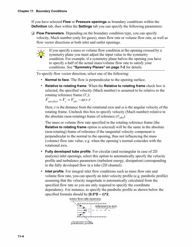
Chapter 11 Boundary Conditions
If you have selected Flow or Pressure openings as boundary conditions within the Definition tab, then within the Settings tab you can specify the following parameters:
Flow Parameters. Depending on the boundary condition type, you can specify velocity, Mach number (only for gases), mass flow rate or volume flow rate, as well as flow vector directions at both inlet and outlet openings.
To specify flow vector direction, select one of the following:• Normal to face. The flow is perpendicular to the opening surface.• Relative to rotating frame. When the Relative to rotating frame check box is
selected, the specified velocity (Mach number) is assumed to be relative to the rotating reference frame (Vr):
.Here, r is the distance from the rotational axis and ω is the angular velocity of the rotating frame. Uncheck this box to specify velocity (Mach number) relative to the absolute (non-rotating) frame of reference (Vabs).The mass or volume flow rate specified in the rotating reference frame (the Relative to rotating frame option is selected) will be the same in the absolute (non-rotating) frame of reference if the tangential velocity component is perpendicular to the normal to the opening, thus not influencing the mass (volume) flow rate value, e.g. when the opening’s normal coincides with the rotational axis.
• Fully developed tube profile. For circular (and rectangular in case of 2D analysis) inlet openings, select this option to automatically specify the velocity profile and turbulence parameters (turbulent energy, dissipation) corresponding to the fully developed flow in a tube (2D channel).
• Inlet profile. For integral inlet flow conditions such as mass flow rate and volume flow rate, you can specify an inlet velocity profile (e.g. parabolic profile) assuming that the velocity magnitude is automatically calculated from the specified flow rate so you are only required to specify the coordinate dependency. For instance, to specify the parabolic profile as shown below the specified formula should be (0.5*D – r)^2.
If you specify a mass or volume flow condition at the opening crossed by a symmetry plane you must adjust the input value to the symmetry condition. For example, if a symmetry plane halves the opening you have to specify a half of the actual mass/volume flow rate to satisfy your conditions. See "Symmetry Planes" on page 7-2 for details.
specified r absV V V rω= = − ×
11-4

• Swirl. Allows you to specify swirling flow about the Reference axis using the Definition tab. You can specify the following vector components of swirl relative to the Reference axis (the swirling direction is defined by the angular velocity sign through the Right-Hand Grip Rule (also known as the Corkscrew Rule)):• Angular velocity (collinear with the Reference axis)• Radial velocity (normal to the Reference axis)• Component normal to face.
• 3D vector. The flow direction is specified through vector components in X, Y, and Z directions with respect to the Coordinate system selected on the Definition tab. Unlike the Velocity condition, for Mass and Volume Flow conditions these components (considered as Relative components) define only flow direction and can be of any arbitrary value. They are automatically recalculated in accordance with the value of the Mass or Volume flow rate normal to face.
Thermodynamic Parameters. The pressure and temperature can be specified at Pressure or inlet Flow openings as follows:
• Static Pressure, Total Pressure or Environment Pressure can be specified at Pressure openings. The Environment pressure condition is interpreted by COSMOSFloWorks as a total pressure for incoming flows and as a static pressure for outgoing flows. If, during calculation, a vortex crosses an opening with the Environment pressure condition specified at it, this pressure considered as the total pressure at the part of opening through which the flow enters the model and as the static pressure at the part of opening through which the flow leaves the model.Additionally, if High Mach number flow is considered (see "Fluid Type and Compressibility" on page 2-4), you need to specify fluid Approximate pressure at inlet Flow openings. See "Boundary Conditions in Gas Analyses" on page 11-9 for explanation of the Approximate pressure parameter.
• Pressure potential. If you enable a rotating reference frame, you can select the Pressure potential check box. When the Pressure potential check box is selected, the specified static pressure is assumed to be relative to the rotating frame pressure (Pr) and the absolute pressure is calculated by the density, angular velocity and the radius:
When the Pressure potential check box is unchecked, the specified static pressure is assumed to be a pressure in terms of the absolute frame of reference (Pabs), i.e. observable by the stationary analyst.If gravitation effects are considered, you can select the Pressure potential check box. When the Pressure potential check box is selected, the specified static pressure is assumed to be piezometric pressure (or potential) and the absolute
2 212specified r absP P P rρω= = − ⋅
Introducing COSMOSFloWorks 11-5

Chapter 11 Boundary Conditions
pressure (Pabs) is calculated using the reference density, gravitational acceleration vector and the position vector:
When the Pressure potential box is unchecked, the specified static pressure is assumed to be an absolute pressure, and the corresponding piezometric pressure is respectively calculated.
• Temperature. Allows you to specify fluid static temperature at Pressure and inlet Flow opening.
Substance Concentrations. For multiple fluids, the relative concentration of each can be specified either by mass or volume. Concentration values specified at Pressure openings are only used if the flow calculation determines that the opening is an inlet.
In addition, click Show advanced parameters if you want to override the default turbulence or boundary layer parameters with your own values:
Turbulence Parameters. The turbulence parameters can be specified at pressure openings and inlet flow openings in terms of turbulent intensity and turbulent length or in terms of turbulent energy and turbulent dissipation. Turbulence parameters specified at Pressure openings are only used if the flow calculation determines that the opening is an inlet. See also "Turbulence" on page 2-5.
Boundary Layer Parameters. For an inlet you can define the Boundary layer type, either laminar or turbulent (turbulent by default), if you have selected Inlet Mass or Volume Flow within the Definition tab, the boundary layer thickness is equal to zero, whereas if you have selected Inlet Velocity within the Definition tab and select Set up boundary layer parameters, you can specify additional boundary layer parameters: thickness of the dynamic and heat boundary layers (Dynamic boundary layer thickness and Heat boundary layer thickness) and the external (with respect to the boundary layer) flow's velocity and temperature (Core velocity and Core temperature). If you set Laminar Only flow in the Wizard or General Settings dialog box then the entire flow field, including the boundary layer, is considered laminar. Boundary layer parameters specified at the pressure opening are used only if the flow calculation determines that the opening is an inlet.
If within the Definition tab you have selected Wall as a boundary condition and Real Wall as a boundary condition type, then within the Settings tab you can specify the following parameters:
Roughness. Select Adjust wall roughness and specify the wall roughness (COSMOSFloWorks uses the Rz value).
Heat transfer coefficient. Select Adjust wall heat transfer coefficient and specify the heat transfer coefficient at the wall, as well as the fluid temperature (and wall temperature if heat transfer is not considered) needed for determining the heat flux from the wall to the fluid through the heat transfer coefficient. This fluid temperature can be specified in two ways:
( )specified piezo abs x y zP P P g x g y g zρ= = − + +
11-6

• As a user defined temperature. Under Define fluid temperature by, select User defined temperature and set the value of the External fluid temperature,
• As the temperature interpolated by COSMOSFloWorks at the specified distance from the wall. Under Define fluid temperature by select Temperature interpolated at prescribed distance, and set the Dynamic boundary layer thickness so the needed fluid temperature is determined from the COSMOSFloWorks calculation at the specified distance from the wall, considered as the dynamic boundary layer’s external boundary.
Wall temperature. Select Adjust wall temperature and specify the wall temperature. The specified wall temperature is considered as a heat source (or sink) regardless of whether “Heat transfer in solids” is considered or not. It is also required if “Heat transfer in solids” is not considered for determining the heat flux from the wall through the heat transfer coefficient.
If you solve an internal problem with “Heat transfer in solids” and have selected Wall as a boundary condition and Outer Wall as a boundary condition type within the Definition tab, then within the Settings tab you can specify a thermal Wall Condition as either wall temperature or heat transfer coefficient at the wall:
Wall temperature. Under Wall Condition select Wall temperature and specify the outer wall temperature.
Heat transfer coefficient. Under Wall Condition, select Heat transfer coefficient and specify the heat transfer coefficient value and the external fluid temperature denoting the heat exchange between the model outer walls and the surrounding fluid as follows:Q = α (Ts-Tf)S.
External fluid temperature is required for determining the heat flux from the model’s external wall to a hypothetical external fluid (surrounding the model) through the specified heat transfer coefficient, at that the required wall temperature is calculated by COSMOSFloWorks when solving an internal problem with “Heat transfer in solids”.
Specifying Moving Wall
The Moving Wall Settings allow you to simulate tangential motion of a wall by specifying the motion direction and the velocity. The available motion types are translation (for cylindrical surfaces) and rotation (for surfaces of revolution). In addition, the stator type can be specified to define a non-rotating wall in case a rotating frame of reference is enabled. The moving wall is treated in the code as the tangential velocity boundary condition at this wall.
To specify a moving wall:
1 In the COSMOSFloWorks analysis tree right-click the Boundary Conditions icon and select Insert Boundary Condition or click FloWorks, Insert, Boundary Condition.
Introducing COSMOSFloWorks 11-7

Chapter 11 Boundary Conditions
2 In the graphics area select the moving surfaces. These faces appear in the Faces to apply the boundary condition list. To remove a face from this list, select it in the list and press Delete, or you can select the face again in the graphics area.
3 Under Basic set of boundary conditions, select Wall.4 Under Type of boundary condition, select Real Wall: the Moving Wall Settings tab
appears.5 Click the Moving Wall Settings tab.6 Select Adjust moving wall settings to specify translation and/or rotation of the wall.
You can simulate the translational motion of the wall along an axis or curve. If the wall does not change its geometry relating to the surrounding fluid, you can also simulate simultaneous translation and rotation of the wall by specifying both the Translation velocity and Angular rotation velocity values.
• Translation. This type of motion can be applied to any cylindrical surface, i.e. a surface created by linear translation (along the generatrix) of a profile curve, to simulate motion along the curve (or along a line in case of a flat face). For a flat wall, the wall motion direction is denoted by the selected reference axis or the axis of the selected coordinate system. For a non-flat cylindrical surface, the surface motion direction is specified tangent to the profile curve.To specify the translational motion of the wall, enter the value of Translation velocity and then specify the Direction of the translation as an axis or curve.
• Rotation. This type of motion can be applied to any surface of revolution, i.e. a surface created by the rotation of a curve, e.g. a cylinder or cone. To specify rotation of the wall, enter the value of Angular rotation velocity and then specify the axis of rotation.
If you select the Relative to rotating frame check box, the velocity values will be specified relative to the rotating reference frame. See also "Rotation" on page 6-12.
7 Select a Motion direction from one of the available types:• Reference Axis. In the FeatureManager tree, select a reference Axis. To create
an axis, go to Insert, Reference Geometry, Axis. For the Translation motion type, the direction of the axis defines the direction of the wall’s motion (if the velocity value is positive). For the Rotation type, the selected axis is assumed to be a rotational axis and the angular velocity obeys the right-handle rule. The axis’ direction is indicated by the axis’ name that is shown near the axis origin.
11-8
• Axis of Coordinate system. In the FeatureManager tree, select a reference Coordinate system (or keep the default Global Coordinate System), then in Axis, select an axis of this coordinate system which either defines the wall direction for the Translation motion type (if the velocity value is positive), or will be a rotation axis for the Rotation motion type (the angular velocity obeys the right-handle rule). To create a reference coordinate system go to Insert, Reference Geometry, Coordinate System.
• Tangent to Curve. In the FeatureManager tree, select a Curve coinciding with the surface’s profile curve to define motion of a cylindrical surface along the profile curve.
8 If you want to specify a stationary (in the absolute, non-rotating reference frame) wall within a local region of rotation or when the global rotating reference frame is enabled, select Stator. When the Stator type of wall is selected, the tangential velocity at this face is equal to zero. See also "Rotation" on page 4-15.
9 Click OK.
Boundary Conditions in Gas Analyses
The following peculiarities of specifying flow boundary conditions should be taken into account if you deal with gas flows.
Inlet ConditionsApproximate pressure. In case of an inlet flow boundary condition (mass flow rate, velocity, Mach number, volume flow rate) in addition to the Temperature, you need to specify the Approximate pressure thermodynamic parameter.The Approximate pressure together with Temperature is used to estimate inlet Mach number, unless you specify Mach number exactly. If inlet Mach number is greater than one (i.e. the inlet flow is supersonic) the Approximate pressure is used as boundary condition and therefore must be specified exactly.If inlet Mach number is less than one, the Approximate pressure is used as an auxiliary parameter only, so it does not influence the converged results but its correct estimation improves the convergence.
Correct use of inlet volume flow, velocity or Mach number conditions.If you specify inlet volume flow or inlet velocity or inlet Mach number condition, and the whole flow stream coming from the opening passes through the sonic velocity, i.e. in the downstream passage the whole flow becomes supersonic (e.g. as in a nozzle flow), the calculation may be incorrect, since the inlet flow conditions (except for the
The reference axis and coordinate system selected on the Definition tab are only used to specify a Dependency and should not be confused with those selected on the Moving Wall Settings tab used for specification of a motion direction.
Introducing COSMOSFloWorks 11-9

Chapter 11 Boundary Conditions
inlet mass flow rate) are fully governed by the gas’s specific heat ratio and the channel’s geometry. As a result, pressure, density and mass flow increase or decrease without any convergence. During such calculations the corresponding warning informs you that in a gas analysis with inlet volume flow, velocity or Mach number condition the flow becomes supersonic somewhere in the computational domain.If you run into such a situation you should instead use an inlet mass flow rate or pressure boundary condition. Note that the problem may only appear if the sonic surface (Mach = 1) totally crosses the passage.
Outlet ConditionsIf you have outlet openings in case of gas flow, and the outlet flow is supersonic, then the boundary condition at the outlet openings, as well as the Ambient downstream boundary for external problems, are ignored.
When specifying outlet boundary conditions, check to see that the corresponding Mach number at this opening is less than one if you want the outlet condition to take effect.
11-10

12 Transferred Boundary Conditions
Creating Transferred Boundary Conditions
The Transferred Boundary Conditions allow you to take results obtained in a previous COSMOSFloWorks calculation as a boundary condition for the current COSMOSFloWorks project.
In Step1 – Selecting Boundaries dialog box you can select the current COSMOSFloWorks project’s boundaries (model faces or Computational Domain boundaries) to apply the Transferred Boundary Conditions.
To create transferred boundary conditions:
1 Click FloWorks, Insert, Transferred Boundary Condition.2 Specify boundaries to apply the transferred boundary condition:
• Select Computational domain boundaries (X max, … Z min) in the corresponding list and click Add (or double-click a boundary), if you want to apply the transferred boundary condition to the Computational Domain boundaries. Boundaries of this type are usually relevant for external analyses, but can be applied to internal analyses also;
• In the graphics area select the model faces (e.g., openings) if you want to transfer boundary condition on these faces. Boundaries of this type are usually relevant for internal analyses, but can be applied to external analyses also;
The selected boundaries appear in the Boundaries to apply the transferred boundary conditions list. To remove a face from the list, select it in the list and press the Delete key.
3 Click Next to select results to transfer. See "Selecting Results to Transfer" on page 12-2.
See also "Transferred Boundary Conditions - Basic Information" on page 3-8.
Introducing COSMOSFloWorks 12-1

Chapter 12 Transferred Boundary Conditions
Selecting Results to Transfer
Allows you to select a COSMOSFloWorks project or flow field (*.fld) file, whose results will be taken as the transferred boundary conditions for the current COSMOSFloWorks project.
To select results to transfer:
1 Select the method in which results are taken:• Select COSMOSFloWorks project, if you want to take the results of a currently
opened model’s project. This is the easiest way to take results obtained earlier in the project of the current model. If you want to take results obtained in another model, you need to open this model first or use the COSMOSFloWorks results (*.fld) file option.
• Select Results (*.fld) file if you want to take the results from a results (*.fld) file from any available COSMOSFloWorks project.
2 Click Browse to select either the desired COSMOSFloWorks project or the desired COSMOSFloWorks results (*.fld) file. As a result, the project (or file) name appears in the Selected COSMOSFloWorks project or results (*.fld) file box.
3 Click Next to specify the type of the transferred condition. See "Specifying Type of Conditions" on page 12-2.
See also "Transferred Boundary Conditions - Basic Information" on page 3-8.
Browse for Project
Allows you to select a project with results used as boundary conditions for the current project at the selected boundaries. If you want to take results obtained in another model, you need to open this model first or use the COSMOSFloWorks results (*.fld) file option.
Specifying Type of Conditions
Allows you to select a type for the transferred boundary condition, i.e., a set of the flow field parameters whose values will be transferred from the selected previous COSMOSFloWorks calculation to the current COSMOSFloWorks project as the transferred boundary condition.
COSMOSFloWorks stores results in the <ProjectNumber>.fld file. This file is stored in the project folder accessible by clicking FloWorks, Project, Open Project Directory. The r_000000.fld file contains results obtained for the zero iteration, i.e. initial computational mesh and initial parameters distribution.
12-2

In the Boundary condition type list you can select one of the following types of flow parameters:
• Ambient – the same flow parameters which are specified at the computational domain boundaries in external analyses; during the calculation they act in the same manner, as in external analyses;
• Impulse – the same flow parameters (fluid temperature, density, substance concentrations, and turbulence parameters) which are specified at the computational domain boundaries in external analyses, with the exception of specifying fluid impulse instead of fluid velocity (both are vectors); during the calculation they act nearly in the same manner, as in external analyses;
• Velocity – the same flow parameters (fluid velocity, temperature, density, substance concentrations, and turbulence parameters) which are specified at the computational domain boundaries in external analyses; during the calculation they act nearly in the same manner, as in external analyses;
• Static pressure – the same flow parameters (static pressure, temperature, substance concentrations, and turbulence parameters) which are specified in the Pressure Openings set of boundary conditions when you select the Static Pressure type of this boundary condition; during the calculation they act nearly in the same manner, as a Pressure-Opening-with-Static-Pressure boundary condition;
• Total pressure – the same flow parameters (total pressure, temperature, substance concentrations, and turbulence parameters) which are specified in the Pressure Openings set of boundary conditions when you select the Total Pressure type of this boundary condition; during the calculation they act nearly in the same manner, as a Pressure-Opening-with-Total-Pressure boundary condition.
Independently of the Transferred Boundary Condition type selected from the above-mentioned variants, if the boundary’s section lies in the solid and Heat Transfer in Solids is enabled in the current COSMOSFloWorks project and was enabled in the COSMOSFloWorks project whose results are taken as the transferred boundary condition, then the solid temperature is taken from this project’s results as the transferred solid boundary condition, whereas the heat flux obtained as the problem’s solution at this boundary depends on the heat transfer in this solid, and in particular can be non-zero.
When specifying boundary conditions for an internal analysis you must take care of their physical compatibility. For example, a project will not run for internal steady-state flows if at model inlets and outlets you specify boundary conditions of the Flow opening type (or Transferred Boundary Condition of the Velocity type) without any boundary condition of the Pressure opening type, so the inlet and outlet mass flow rates are not balanced exactly.
Introducing COSMOSFloWorks 12-3

Chapter 12 Transferred Boundary Conditions
To avoid such problems we recommend that you specify at least one pressure condition (Boundary Condition of the Pressure Opening type or Transferred Boundary Condition of the Static (Total) Pressure type) and at least one Boundary Condition of the Flow Opening type or Transferred Boundary Condition of the Velocity (or Impulse) type.
Click Finish to accept and save the settings made in the Transferred Boundary Conditions wizard and close the wizard.
12-4

13 Fans
Creating a Fan
Allows you to include a fan specified in the Engineering Database as an ideal device creating a volume (or mass) flow rate. The rate depends on the difference between the average inlet static pressure and the average outlet static pressure (the averages are calculated over the fan inlet and outlet sections). You apply the fan to model faces, including model inlet and outlet openings closed with auxiliary lids (see "How It Works" on page 1-1). You can use a Fan in both Internal and External flow analyses. For more general information see "Fans – Basic Information" on page 3-10.
You can visualize specified fans directly on the SolidWorks model: colored arrows indicate the direction and type of condition. Right-click a fan item in the COSMOSFloWorks analysis tree and select Show or Hide to turn on or turn off the arrows.
To create a fan:
1 Click Fan on the COSMOSFloWorks Features toolbar or FloWorks, Insert, Fan.– or –In the COSMOSFloWorks analysis tree right-click the Fans icon and select Insert Fan.
2 Click Browse and select the appropriate Fan curve among the list of fans currently available in the Engineering Database.
3 In the Fan type list select the required fan type: External Inlet Fan, External Outlet Fan, and Internal Fan. Terms are described below.
• Inlet denotes injection of the fluid from the fan into the fluid volume.• Outlet denotes suction of the fluid by the fan from the fluid volume.• External denotes that the fan is installed at a model inlet or outlet opening.
Introducing COSMOSFloWorks 13-1

Chapter 13 Fans
• Internal. Since both sides of an Internal Fan are in contact with the fluid, the fluid static pressure difference between the sides governs fluid passage in accordance with the specified fan type.
4 Select faces on which you intend to specify fan. For an Internal Fan, prior to selecting faces, you must click the corresponding (Inlet or Outlet) Faces to apply list. To remove a face from the Faces to apply list, select it in the list and press the Delete key or select the face again in the graphics area. You can also click Filter to remove faces of the specified type from the selection list. See "Selection Filter" on page 22-17 for details.
5 If you intend to specify either a fluid swirl or 3D velocity vectors, or non-uniform flow parameter distributions on a model face, select a reference Coordinate system. The default coordinate system selected is:• Face based coordinate system (for single planar faces). This coordinate system is
located at the center of the face with the X-axis oriented normally to the plane. • Global Coordinate System (for surfaces or if more than one planar face is
selected).You can replace the default coordinate system by selecting your coordinate system in the FeatureManager tree. To create a coordinate system, click Insert, Reference Geometry, Coordinate System.
6 To reference a cylindrical coordinate system, select an axis of the specified Coordinate system in the Reference axis list. The selected Coordinate system and Reference axis also define a local spherical coordinate system.
7 COSMOSFloWorks allows you to associate a fan type with a goal(s), which will be automatically created with the fan condition if the Create associated goals check box is selected. You can associate goals with a fan type under the Automatic Goals item of the General Options dialog box.
8 Click the Settings tab and specify parameter values for the selected fan type.9 Click OK. The new fan item appears in the Analysis Tree. To edit definition of a fan,
in the COSMOSFloWorks analysis tree, double-click the fan item, or right-click the item and select Edit Definition.
If you specify an Internal Fan, remember that Inlet faces are openings through which flow exits from the fan and Outlet faces are openings through which flow enters the fan.
13-2
Specifying Fan Parameters
Allows you to complete the definition of a fan by specifying an appropriate flow parameters, thermodynamic parameters, concentration (for multiple fluids), and turbulence parameters.Double-click a Value cell to edit the cell contents or select the appropriate parameter type. If you want to specify a coordinate-dependent or time-dependent value, click the corresponding Value box and click Dependency. See "Dependency" on page 22-1 for details.
Relative to rotating frame. The volume (or mass) flow rate produced by the fan in the rotating reference frame (the Relative to rotating frame option is selected) will be the same in the absolute (non-rotating) frame of reference if the tangential velocity component is perpendicular to the normal to the opening, thus not influencing the volume (mass) flow rate value, e.g. when the opening’s normal coincides with the rotational axis. For details about the rotating reference frame see "Rotation" on page 6-12.
Flow Parameters. Allows you to specify the flow direction at faces selected as inlet or outlet. For an Internal fan you specify flow direction at inlets as Inlet flow parameters and at outlets as Outlet flow parameters. To specify flow direction in the Flow vectors direction list select one the following:
• Normal to face. The flow is perpendicular to the face selected as inlet or outlet.• Swirl. Allows you to specify swirling flow about the Reference axis selected by
using the Definition tab. You can specify the following vector components of swirl relative to the Reference axis (the swirling direction is defined by the angular velocity sign through the Right-Hand Grip Rule (also known as the Corkscrew Rule)):Angular velocity (collinear with the Reference axis)Radial velocity (normal to the Reference axis)
• 3D vector. The flow direction is specified through vector components in X, Y, and Z directions with respect to the Coordinate system selected on the Definition tab.
Thermodynamic Parameters.• Ambient pressure. For an External Inlet or Outlet Fan you specify a total
pressure outside the model. The difference between this pressure and the fluid pressure governs the fluid injection (External Inlet) or suction (External Outlet) according to the selected Fan Curve.
• Temperature. Allows you to specify static temperature of the fluid that flows out from the fan. For an Internal Fan, clear the Use outlet temperature check box if you want to enforce heating or cooling of the fluid inside the fan by specifying the desired temperature of the fluid exiting the fan.
Introducing COSMOSFloWorks 13-3

Chapter 13 Fans
Substance Concentrations. For multiple fluids the relative concentration can be specified either by mass or by volume.
For an External Inlet Fan or Internal Fan click Show advanced parameters if you want to override the default turbulence parameters with your own values.
Turbulence Parameters. The turbulence parameters can be specified in terms of turbulent intensity and turbulent length or in terms of turbulent energy and turbulent dissipation. See also "Turbulence" on page 2-5. For an Internal Fan clear the Use outlet turbulence check box if you want to specify turbulence parameters of the flow exiting the fan that are different from the turbulence parameters of the flow entering the fan.
13-4

14 Heat Sources
Creating a Surface Source
Allows you to specify a heat surface source on a surface in contact with the fluid as well as on a surface that is boundary between solids.
If you do not consider Heat Conduction in Solids, this source (in the form of Heat Transfer Rate, or Heat Flux) is a thermal wall boundary condition for the fluid. It is specified on the selected faces and overrides the Default Wall Conditions for the selected faces.
If you consider Heat Conduction in Solids, a surface source in the form of Heat Generation Rate, or Surface Heat Generation Rate serve as a heat source on a solid surface (see below).
To create a surface source:
1 Click Surface Source on the COSMOSFloWorks Features toolbar or FloWorks, Insert, Surface Source.– or –In the COSMOSFloWorks analysis tree, right-click the Heat Sources item and select Insert Surface Source.
2 In the Source type list select the appropriate source type from the following types: If Heat transfer in solids is disabled:
• Heat Transfer Rate (W), Heat Flux (W/m2). The heat flow from solid to fluid is governed by the specified Heat Transfer Rate (Heat Flux) value.
If Heat transfer in solids is enabled:• Heat Generation Rate (W), Surface Heat Generation Rate (W/m2). The
heat flow from the fluid to the solid is governed by the surface temperature, which is a function of the specified Heat Generation Rate (Surface Heat Generation Rate) and the solid conduction. In other words, depending on the
Introducing COSMOSFloWorks 14-1

Chapter 14 Heat Sources
intensity of the solid conduction near the surface and the specified value of the Heat Generation Rate (Surface Heat Generation Rate) the surface temperature changes resulting in changes in heat flow.
3 In the graphics area select the model faces, on which you intend to specify the surface source. These faces appear in the Faces to apply the surface source list. To remove a face from this list, select it in the list and click Remove or you can select the face again in the graphics area. You can also click Filter to remove faces of the specified type from the selection list. See "Selection Filter" on page 17-17 for details.
4 If you intend to specify a non-uniform thermal parameter distribution on the selected surface, select a reference Coordinate system. By default, the Global Coordinate System is selected. You can replace the default coordinate system by selecting your coordinate system in the FeatureManager tree. To create a coordinate system click Insert, Reference Geometry, Coordinate System.
5 To reference a cylindrical coordinate system, in the Reference axis list select an axis of the specified Coordinate system. The selected Coordinate system and Reference axis also define a local spherical coordinate system.
6 COSMOSFloWorks allows you to associate a surface source type with a goal(s), which will be automatically created together with the surface source if the Create associated goals check box is selected. You can associate goals with a surface source type under the Automatic Goals item of the General Options dialog box.
7 Under Settings specify value for the selected source.8 Click OK. The new surface source item (SS) appears in the analysis tree. To edit
definition of a surface source, in the COSMOSFloWorks analysis tree, double-click the surface source item, or right-click the item and select Edit Definition.
Creating a Volume Source
Allows you to specify a heat volume source in solid or in fluid.
• The volume source in solid can be only specified if you consider Heat Conduction in Solids.
• To specify a volume source in fluid, a component (a part or subassembly in assemblies, as well as a body in multibody parts) must be used to represent the volume of the fluid region. Additionally, the component must be disabled via the Component Control dialog box. Once disabled, the component is treated as a fluid substance in which you can specify an internal fluid thermal source.
If you specify Heat Generation Rate in a body, some part of which is outside the Computational Domain, then in the analysis the heat generation rate will be proportional to the body’s volume protruding inside the computational domain.
14-2

To create a volume source:
1 Click Volume Source on the COSMOSFloWorks Features toolbar or FloWorks, Insert, Volume Source.– or –In the COSMOSFloWorks analysis tree, right-click the Heat Sources item and select Insert Volume Source.
2 In the Source type list select the appropriate source type from the following three types: Heat Generation Rate (W), Volumetric Heat Generation Rate ( ), and Temperature.
3 In the graphics area, click a face, edge or point to select a component. You can also select a component in the FeatureManager tree. These components appear in the Components to apply the volume source list. To remove a component from this list, select it in the list and click Remove.
4 If you intend to specify a non-uniform thermal parameter distribution in the selected component, select a reference Coordinate system. By default, the Global Coordinate System is selected. You can replace the default coordinate system by selecting your coordinate system in the FeatureManager tree. To create a coordinate system click Insert, Reference Geometry, Coordinate System.
5 To reference a cylindrical coordinate system, in the Reference axis list select an axis of the specified Coordinate system. The selected Coordinate system and Reference axis also define a local spherical coordinate system.
6 COSMOSFloWorks allows you to associate a volume source type with a goal(s), which will be automatically created together with the volume source if the Create associated goals check box is selected. You can associate goals with a surface source type under the Automatic Goals item of the General Options dialog box.
7 Under Settings specify value for the selected source.A positive value of the Heat generation rate or Volumetric heat generation rate denotes a heat generation in the volume. A negative value denotes the heat absorption.Click Dependency to specify a coordinate-dependent or time-dependent value.
8 Select the Disable solid components option if you want to disable the component in which the volume source is specified. COSMOSFloWorks treats the disabled component as the fluid volume.
9 Click OK. The new volume source item (VS) appears in the analysis tree. To edit definition of a volume source, in the COSMOSFloWorks analysis tree, double-click the volume source item, or right-click the item and select Edit Definition.
Wm3-------
Introducing COSMOSFloWorks 14-3

Chapter 14 Heat Sources
14-4

15 Radiative Surfaces
Creating a Radiative Surface
Creating a radiative surface allows you to consider a surface in contact with the fluid as a radiative surface, for a conjugate heat transfer problem with the Radiation option enabled.
To create a radiative surface:
1 Click Radiative Surface on the COSMOSFloWorks Features toolbar or FloWorks, Insert, Radiative Surface.– or –In the COSMOSFloWorks analysis tree, right-click the Radiative Surfaces icon and select Insert Radiative Surface.
2 Click Browse and select the desired radiative surface from the list of surfaces, which are currently available in the Engineering Database. See "Surface-to-surface Radiation" on page 2-10 for more details about the radiative surface properties.
3 In the graphics area select the faces on which you intend to specify the radiative surface. These faces appear in the Faces to apply the radiative surface list. To remove a face from this list, select it in the list and press the Delete key or select the face again in the graphics area.You can also click Filter to remove faces of the specified type from the selection list. See "Selection Filter" on page 22-17 for details.
4 If you have selected an opening/outer boundary radiative surface, specify the Radiative temperature (Tr) denoting the heat radiated from this surface into the model or computational domain as follows: Q = εσTr
4.5 If you selected the solar opening radiative surface, specify the direction vector
(through the vector Direction X, Y, Z components) and the radiation Intensity denoting
Any radiative surface type except for the non-radiating surface applied to an insulator's wall will be automatically changed by the program to the whitebody wall.
Introducing COSMOSFloWorks 15-1

Chapter 15 Radiative Surfaces
the directional heat radiation from this surface into the model or computational domain. For time-dependent analysis, click Dependency to specify the radiation Intensity and Direction as a function of time.
6 COSMOSFloWorks allows you to associate a radiative surface type with a goal(s), which will be automatically created with the radiative surface condition if the Create associated goals check box is selected. You can associate goals with a radiative surface type under the Automatic Goals item of the General Options dialog box.
7 Click OK. The new radiative surface item appears in the Analysis Tree. To edit the definition of a radiative surface, in the COSMOSFloWorks analysis tree, double-click the radiative surface item, or right-click the item and select Edit Definition.
15-2

16 Contact Resistances
Creating a Contact Resistance
If you are solving a problem that uses the Heat conduction in solids option, you can specify the thermal contact resistance at the solid/solid and the solid/fluid boundaries. Thermal contact resistance can be specified either by inputting the value of thermal contact conductance or by inputting the thickness and material of the contact layer. In the latter case, the thermal resistance of the contact layer is calculated using the following formula:
where dc is the contact layer’s thickness and λc is the thermal conductivity of contact layer’s material.
To create a contact resistance:
1 Click Contact Resistance on the COSMOSFloWorks Features toolbar or click FloWorks, Insert, Contact Resistance– or –In the COSMOSFloWorks analysis tree right-click the Contact Resistances icon and select Insert Contact Resistance.
2 In the Contact resistance type list select the desired contact resistance type.3 If you have selected a Solid material/thickness type of contact resistance, specify the
following parameters:
Only this ratio is used in the calculation. The contact layer is considered as
infinitely thin and the specified thickness is used to calculate the ratio
only. Therefore, temperature has a discontinuity at the contact surface.
c
cCi
dRλ
=,
c
cdλ
Introducing COSMOSFloWorks 16-1

Chapter 16 Contact Resistances
• Material thickness is a thickness of the contact layer material. Click Dependency if you want to specify coordinate-dependent or time-dependent values. See "Dependency" on page 22-1 for details.
• Solid material is the material of the contact layer. Click Browse and select the desired material from the list of solid materials in the Engineering Database.
4 If you have selected the Contact conductance type of contact resistance, click Browse and select the desired Contact conductance from the list of available values of contact conductance (for various materials) in the Engineering Database.
5 In the graphics area select the model faces on which you want to specify the contact resistance. These faces appear in the Faces to apply contact resistance list. To remove a face from this list, select it in the list and click Remove or select the face again in the graphics area. You can also click Filter Faces to remove faces of the specified type from the selection list. See "Selection Filter" on page 22-17 for details.
6 Click OK. The new Contact Resistance item appears in the COSMOSFloWorks Analysis Tree. To edit the definition of a contact resistance, in the COSMOSFloWorks analysis tree, double-click the Contact Resistances item, or right-click the item and select Edit Definition.
16-2
17 Heat Sink Simulations
Creating a Heat Sink Simulation
The Heat sink simulation feature allows you to simulate a heat sink of a complex shape using a simple parallelepiped. It is convenient for analyzing fluid flow and heat transfer in electronics enclosures containing many components. By replacing a complex shape heat sink with a heat sink simulation, you can reduce the computational time for such problems.
The Heat sink simulation feature is considered a parallelepiped-shaped component with fluid entering through one selected face and leaving through other selected faces. Heat is generated within a component with specified Heat generation rate. Also, a Fan curve and Heat resistance curve must be specified for the heat sink simulation by selecting the fan and heat sink items from the Engineering Database (see "Engineering Database" on page 22-3).
To create a heat sink simulation:
1 Click Heat Sink Simulation on the COSMOSFloWorks Features toolbar or click FloWorks, Insert, Heat Sink Simulation.– or –In the COSMOSFloWorks analysis tree right-click the Heat Sink Simulations icon and select Insert Heat Sink Simulation.
2 Click Browse and select the appropriate Fan curve from the list of Fan Curves currently available in the Engineering Database.
3 Click Browse and select the appropriate Thermal resistance and pressure drop curve from the list of Heat Sinks currently available in the Engineering Database.
4 Specify a Heat generation rate for the heat sink. For time-dependent analysis, click Dependency to define the Heat generation rate as a function of time. See "Dependency" on page 22-1 for details.
Introducing COSMOSFloWorks 17-1

Chapter 17 Heat Sink Simulations
5 In the graphics area click a face, edge or a point to select a component for which you want to specify the Heat sink. You can also select a component in the FeatureManager tree. These components appear in the Components to apply heat sink simulation list. To remove a component from this list, select it in the list and press the Delete key.
6 Click in the Faces the fluid enters the exchanger list box. In the graphics area select the model faces substituting for the inlet of the simulated heat sink’s fan through which fluid enters the heat sink. These faces appear in the Faces the fluid enters the exchanger list. To remove a face from this list, select it in the list and press the Delete key or select the face again in the graphics area.
7 Click in the Faces the fluid exits the exchanger list box. In the graphics area select the model faces through which fluid leaves the heat sink. These faces appear in the Faces the fluid exits the exchanger list. To remove a face from this list, select it in the list and press the Delete key or select the face again in the graphics area.
8 Click OK. The new Heat Sink Simulation item appears in the COSMOSFloWorks Analysis Tree. To edit the definition of a heat sink simulation, in the COSMOSFloWorks analysis tree, double-click the Heat Sink Simulation item, or right-click the item and select Edit Definition.
17-2

18 Porous Media
Creating a Porous Medium
Allows you to consider a component (a part or subassembly in assemblies, as well as a body in multibody parts) as a porous medium. The available porous media are taken from the Engineering Database. A porous medium cannot be created if the High Mach number flow option is enabled.
Before creating a porous medium go to the Engineering Database and define the porous medium you want to use.
The component representing the porous substance must be disabled. Therefore the Porous Medium condition automatically disables this component. Note that components stay disabled after you delete the Porous Medium.
To create a porous medium:
1 Click Porous Medium on the COSMOSFloWorks Features toolbar or FloWorks, Insert, Porous Medium.– or –In the COSMOSFloWorks analysis tree, right-click the Porous Media icon and select Insert Porous Medium.
2 In the FeatureManager tree select a component which you want to consider as the porous medium. You can also click a face, edge or point in the graphics area to select a component. The selected components appear in the Components to apply the porous medium list. To remove a component from this list, select it in the list and press the Delete key.
3 Click Browse and select the desired porous medium from the list of media, which are available in the Engineering Database.
Introducing COSMOSFloWorks 18-1
Chapter 18 Porous Media
4 If you have selected a non-isotropic porous media (Unidirectional, Axisymmetrical, Orthotropic), click the Direction tab and specify the necessary axis or coordinate system to complete the definition of the porous media.
5 Click OK. The new porous medium item appears in the COSMOSFloWorks Analysis Tree. To edit the definition of a porous medium, in the COSMOSFloWorks analysis tree, double-click the porous medium item, or right-click the item and select Edit Definition.
Specifying Porous Medium Parameters
Allows you to specify characteristic directions for non-isotropic porous media. In the Engineering Database the non-isotropic porous medium's properties are specified in abstract direction. Here, you complete the definition of a non-isotropic porous medium by applying concrete directions
For the Unidirectional and Axisymmetrical types of porous media you can select the main direction in two ways:
• Direction is one of the axes of the selected coordinate system. Allows you to specify the characteristic direction as the Reference axis of the selected Coordinate system. By default, the Global Coordinate System is selected. You can replace the Global Coordinate System by selecting your coordinate system in the FeatureManager tree. To create a coordinate system click Insert, Reference Geometry, Coordinate System.
• Direction is the tangent to the selected curve everywhere. Allows you to specify the characteristic direction that is tangent to the selected Curve at any point. To select a curve, click the curve feature in the FeatureManager tree.
For the Orthotropic type of porous media, three mutually perpendicular characteristic directions are parallel to the axes of the selected Coordinate system. You can create your own coordinate system oriented to coincide with the porous medium's characteristic directions and replace the default Global Coordinate System by selecting the coordinate system feature in the FeatureManager tree. To create a coordinate system click Insert, Reference Geometry, Coordinate System.
18-2

19 Initial Conditions
Creating an Initial Condition
Creating an initial condition allows you to specify:
Initial flow and/or temperature conditions in specific fluid regions that differ from the default initial conditions specified in Wizard or General Settings. In this case, a component (a part or subassembly in assemblies, as well as a body in multibody parts) must be used to represent the volume of the fluid region. Additionally, the component must be disabled via the Component Control dialog box or by selecting the Disable solid components option in the Initial Condition dialog box. Once disabled, the component is treated as a fluid substance for which you can specify initial velocity or Mach number, pressure, temperature, density, concentrations (for multiple fluids) and turbulence parameters.
An initial solid temperature for one or more components in a conjugate heat transfer problem. See also "Heat Conduction in Solids" on page 2-2.
To create a initial condition:
1 Click Initial Condition on the COSMOSFloWorks Features toolbar or FloWorks, Insert, Initial Condition.– or –In the COSMOSFloWorks analysis tree right-click the Initial Conditions icon and select Insert Initial Condition.
2 In the graphics area click a face, edge or point to select a component for which you want to specify the initial condition. You can also select a component in the FeatureManager tree. These components appear in the Components/faces to apply the initial condition list. To remove a component from this list, select it in the list and press the Delete key.If you want to specify an initial condition to a fluid region within a closed internal fluid volume, instead of creating this volume as a separate component (and disabling
Introducing COSMOSFloWorks 19-1

Chapter 19 Initial Conditions
it), you can select any surface bounding this fluid volume to be automatically considered by the program as the volume to apply the fluid initial conditions.
3 If you intend to specify either gas initial conditions or a non-uniform solid temperature distribution, select a reference Coordinate system. By default, the Global Coordinate System is selected. You can replace the default coordinate system by selecting your coordinate system in the FeatureManager tree. To create a coordinate system click Insert, Reference Geometry, Coordinate System.
4 To reference a cylindrical coordinate system, select the axis of the specified Coordinate system in the Reference axis list. The selected Coordinate System and Reference axis also define a local spherical coordinate system.
5 Click the Settings tab and specify parameters for the selected components.6 Click OK. The new initial condition item appears in the Analysis Tree. To edit
definition of an initial condition, in the COSMOSFloWorks analysis tree, double-click the initial condition item, or right-click the item and select Edit Definition.
See also "Initial Conditions – Basic Information" on page 3-4.
Specifying Initial Condition Parameters
Depending on the component state (as fluid or solid, which can be changed in Component Control) you can specify either an initial flow parameters distribution or initial solid temperature. For the selected fluid volume you can specify an initial flow parameters distribution.
Double-click a Value cell to edit the cell contents or select the appropriate parameter type. If you want to specify a coordinate-dependent or time-dependent value, click the corresponding Value box and click Dependency. See "Dependency" on page 22-1 for details.
The following parameters can be specified for the selected fluid volume or components, which are treated as a fluid (disabled in Component Control or by selecting the Disable solid components option in the Initial Condition dialog box):
• Flow Parameters. Allows you to specify initial Velocity vector or Mach Number vector (only for gases) through its X-, Y-, and Z-components with respect to the Coordinate system selected on the Definition tab.
• Thermodynamic Parameters. The initial static pressure, static temperature and static density can be specified for gases, and only static pressure and static temperature for liquids. Under Type of thermodynamic parameters definition, select a pair of independent thermodynamic parameters and the third parameter is calculated automatically.
• Substance Concentrations. For multiple fluids the relative concentration can be specified either by mass or by volume.
19-2

Click Show advanced parameters if you wish to override the default turbulence parameters with your own values.
• Turbulence Parameters. The turbulence parameters can be specified in terms of turbulence intensity and turbulence length or in terms of turbulent energy and turbulent dissipation. See also "Turbulence" on page 2-5.
Under Solid Parameters you can specify the initial solid Temperature for the selected solid components (enabled in Component Control).
Introducing COSMOSFloWorks 19-3

Chapter 19 Initial Conditions
19-4

20 Goals
Global Goal
Allows you to specify global goals for your project. A global goal is a physical parameter calculated in the entire computational domain. For more general information, see also "Goals – Basic Information" on page 1-5.
To specify a global goal:
1 Click Global Goal on the COSMOSFloWorks Features toolbar or FloWorks, Insert, Global Goals.– or –In the COSMOSFloWorks analysis tree, right-click the Goals icon and select Insert Global Goals.
2 In the Parameter table select a parameters of interest. For non-integral parameters (e.g. static pressure, or total pressure, etc.) select which parameter value, minimum (Min), average (Av), maximum (Max) or bulk average (Bulk Av) (calculated within the entire Computational Domain) will be used as the global goal.
Average
Bulk Average
Here, Ai is the averaged parameter (e.g. temperature), dVi – the volume of i-th cell, ρi – density in i-th cell and the summation is taken over all the cells within the computational domain.
i icells
icells
A dV
V
⋅∑∑
i i icells
i icells
A dV
V
ρ
ρ
⋅∑∑
Introducing COSMOSFloWorks 20-1

Chapter 20 Goals
3 Select the Use for convergence control (Use for Conv) check box if you want the goal’s convergence to be included as a condition of finishing the calculation. If you clear this check box, the goal’s convergence is used for information only so the calculation may be stopped before the goal is converged. See "Finishing the Calculation" on page 23-2. The yellow-red icon in the COSMOSFloWorks analysis tree indicates goals that have no influence on the task convergence. Also, these goals do not have a progress bar in the Goal Plot and Goal Table monitor dialog boxes.
4 For the X(Y, Z) - Component of Force and X(Y, Z) - Component of Torque goals you can select the Coordinate system in which these goals are calculated. By default, the Global Coordinate System is selected. You can replace the default coordinate system by selecting your coordinate system in the FeatureManager tree. To create a coordinate system click Insert, Reference Geometry, Coordinate System.
5 In the Name template box you can specify a template for names of goals that will be created for selected parameters. The default template is an abbreviated name of goal’s type (GG for Global goals) followed by <Parameter> and <Number>, where <Parameter> is the goal parameter and <Number> is a sequential number of the goal. When goals are created, <Parameter> is replaced by the goal parameter’s name (e.g. Av Static Pressure) and <Number> is replaced by a sequential number of the goal (for example, if the goal named GG Av Static Pressure 1 already exists, the new goal will be named GG Av Static Pressure 2 and so on). You can combine these standard elements in any order and add any appropriate characters to the template. To add a new standard element to the template, click the Parameter or Number button.
6 Click OK. The new global goal items (GG) appear in the Analysis Tree. To edit definition of a global goal, in the COSMOSFloWorks analysis tree, double-click the global goal item, or right-click the item and select Edit Definition.
Surface Goal
Allows you to specify surface goals for your project. A surface goal is a physical parameter calculated on the selected surfaces.
The surface can be any face either contacting with the fluid (a model wall or an opening) or arranged in the fluid (a face of a model component disabled in Component Control dialog box). For more general information, see also "Goals – Basic Information" on page 1-5.
To specify a surface goal:
1 Click Surface Goal on the COSMOSFloWorks Features toolbar or FloWorks, Insert, Surface Goals.– or –In the COSMOSFloWorks analysis tree, right-click the Goals icon and select Insert Surface Goals.
20-2

2 In the Parameter table select a parameter of interest. For non-integral parameters (e.g. static pressure, or total pressure, etc.) select which parameter value, minimum (Min), average (Av), maximum (Max) or Bulk Average (Bulk Av) (calculated on the selected faces) will be used as the surface goal.
Average
Bulk Average
Here, Ai is the averaged parameter (e.g. temperature), dSi – the intersection area of i-th cell, ρi – density in i-th cell, vi – the normal to the surface velocity component in the i-th cells and the summation is taken over all the cells intersecting with the surface.Unlike the Average value which considers only the surface area, the Bulk Average is a value averaged over the core of the flow through the surface, i.e. considering the mass flow rate as well. For example, you are interested in the temperature of an incompressible fluid flowing through a tube’s opening so the flow core is quite hot compared to the low velocity near-wall flow. Thus, most of the hot fluid is concentrated in the center of the flow. If you now calculate the Average value, the cool fluid cells near the wall will be accounted equally within the average value and if the total area of the near-wall cells (with low temperature) is considerable with respect to the opening area, the obtained average value will be lower than the value you could receive in reality, for instance from the experiment. If you take the Bulk Average value, the obtained temperature will be higher in this case since the cool near-wall cells with a lower mass flow rate has less influence than the much hotter with larger mass flow rate region near the core (free stream) of the flow.
3 In the graphics area select faces on which you intend to specify the surface goal. These faces appear in the Faces to apply the surface goal list. To remove a face from this list, select it in the list and click Remove or select the face again in the graphics area. You can also click Filter to remove faces of the specified type from the selection list. See "Selection Filter" on page 22-17 for details.TIP: To quickly select faces on which you have specified a boundary condition, fan or surface source, select the corresponding feature in the COSMOSFloWorks analysis tree. All faces belonging to the feature will be automatically selected.
4 Select the Use for convergence control (Use for Conv) check box if you want the goal’s convergence to be included as a condition of finishing the calculation. If you clear this check box, the goal’s convergence is used for information only so the
You can also right-click a model face in the graphics area and select Insert Surface Goal to create a surface goal on the face.
i icells
icells
A dS
S
⋅∑∑
i i i icells
i i icells
A v dS
v S
ρ
ρ
⋅∑∑
Introducing COSMOSFloWorks 20-3

Chapter 20 Goals
calculation may be stopped before the goal is converged. See "Finishing the Calculation" on page 23-2.The yellow-red icon in the COSMOSFloWorks analysis tree indicates goals that have no influence on the task convergence. Also, such goals do not have the progress bar in the Goal Plot and Goal Table monitor dialog boxes.
5 For the X(Y, Z) - Component of Force and X(Y, Z) - Component of Torque goals you can select the Coordinate system in which these goals are calculated. By default, the Global Coordinate System is selected. You can replace the default coordinate system by selecting your coordinate system in the FeatureManager tree. To create a coordinate system click Insert, Reference Geometry, Coordinate System.For forces set on non-closed surfaces, the actual force value is the obtained goal value plus the Reference Pressure multiplied by the surface area. The Reference Pressure value can be viewed in the Results Summary
6 In the Name template box you can specify a template for names of goals that will be created for selected parameters. The default template is an abbreviated name of goal’s type (SG for Surface goals) followed by <Parameter> and <Number>, where <Parameter> is the goal parameter and <Number> is a sequential number of the goal. When goals are created <Parameter> is replaced by the goal parameter’s name (e.g. Av Static Pressure) and <Number> is replaced by a sequential number of the goal (for example, if the goal named SG Av Static Pressure 1 already exists, the new goal will be named SG Av Static Pressure 2 and so on). You can also add words “Inlet” or “Outlet” to the template by clicking the corresponding button. You can combine these standard elements in any order and add any appropriate characters to the template. To add a new standard element to the template, click the Inlet, Outlet, Parameter or Number button.
7 Click OK. The new surface goal items (SG) appear in the Analysis Tree. To edit definition of a surface goal, in the COSMOSFloWorks analysis tree, double-click the surface goal item, or right-click the item and select Edit Definition.
Volume Goal
Allows you to specify volume goals of your project. A volume goal is a physical parameter calculated within specified volumes (part or subassembly components in assemblies, as well as bodies in multibody parts) inside the Computational Domain.
Parameters are calculated in fluid or solid depending on the component state (as fluid or solid, which can be changed in Component Control). If you do not consider Heat Transfer in Solids, then no parameters are valid for calculation in a solid, otherwise temperature is the only valid parameter.
For more general information, see also "Goals – Basic Information" on page 1-5.
To specify a volume goal:
1 Click Volume Goal on the COSMOSFloWorks Features toolbar or FloWorks, Insert, Volume Goals.
20-4

– or –In the COSMOSFloWorks analysis tree, right-click the Goals icon and select Insert Volume Goals.
2 In the graphics area click a face, edge or a point to select a component for which you want to specify the volume goal. You can also select a component in the FeatureManager tree. These components appear in the Components to apply the volume goal list. To remove a component from this list, select it in the list and click Remove.TIP: To quickly select components on which you have specified an initial condition, or volume source, select corresponding feature in the COSMOSFloWorks analysis tree and all the components belonging to the feature will be automatically selected.
3 In the Parameters table select a parameter of interest. For non-integral parameters (e.g. static pressure, or total pressure, etc.) select which parameter value, minimum (Min), average (Av), maximum (Max) or Bulk Average (Bulk Av) (all calculated within the selected components) will be used as the volume goal.
Average
Bulk Average
Here, Ai is the averaged parameter (e.g. temperature), dVi – the volume of i-th cell, ρi – density in i-th cell and the summation is taken over the cells within the selected component (volume).
4 Select the Use for convergence control (Use for Conv) check box if you want the goal’s convergence to be included as a condition of finishing the calculation. If you clear this check box, the goal’s convergence is used for information only so the calculation may be stopped before the goal is converged. See "Finishing the Calculation" on page 23-2.The yellow-red icon in the COSMOSFloWorks analysis tree indicates goals that have no influence on the task convergence. Also, such goals do not have the progress bar in the Goal Plot and Goal Table monitor dialog boxes.
5 In the Name template box you can specify a template for names of goals that will be created for selected parameters. The default template is an abbreviated name of goal’s type (VG for Volume goals) followed by <Parameter> and <Number>, where <Parameter> is the goal parameter and <Number> is a sequential number of the goal. When goals are created, <Parameter> is replaced by the goal parameter’s name (e.g. Max Temperature of Fluid) and <Number> is replaced by a sequential number of the goal (for example, if the goal named VG Max Temperature of Fluid 1 already exists,
i icells
icells
A dV
V
⋅∑∑
i i icells
i icells
A dV
V
ρ
ρ
⋅∑∑
Introducing COSMOSFloWorks 20-5

Chapter 20 Goals
the new goal will be named VG Max Temperature of Fluid 2 and so on). You can combine these standard elements in any order and add any appropriate characters to the template. To add a new standard element to the template, click the Parameter or Number button.
6 Click OK. The new volume goal items (VG) appear in the Analysis Tree. To edit definition of a volume goal, in the COSMOSFloWorks analysis tree, double-click the volume goal item, or right-click the item and select Edit Definition.
Equation Goal
Allows you to specify a goal defined by an equation (basic mathematical functions) with the existing goals or parameters of input data conditions (boundary conditions, fans, initial conditions, etc.) as variables. This goal can be viewed as an equation goal during the calculation and while displaying results in the same way as the other goals. As variables, you can use any of the specified goals including another equation goal except for the goals that are dependent from other equation goals, and parameters of the specified project's input data features (initial or ambient conditions, boundary conditions, fans, heat sources, local initial conditions). You can also use constants in the definition of the equation goal.
The equation goal is convenient because it allows COSMOSFloWorks to calculate the parameter of interest (i.e., pressure drop) and keeps this information in the project for later reference.
To create an equation goal:
1 Click Equation Goal on the COSMOSFloWorks Features toolbar or FloWorks, Insert, Equation Goal.- or -In the COSMOSFloWorks analysis tree, right-click the Goals icon and select Insert Equation Goal.
2 In the COSMOSFloWorks Analysis tree, click the goal or input data feature whose parameter you want to use in the equation. To select parameters of initial and ambient (for external analyses) or initial (for internal analyses) conditions (those specified in General Settings), click the Input Data item. The selected goal appears in the Expression box defining the equation goal, while if you select an input data feature other than goal its parameters appear in the Parameter list. In the latter case, select the desired parameter in the Parameter list to add the parameter into the Expression box.For transient analyses, you can add a physical time as a parameter to the equation by clicking the Physical Time button.
20-6
TIP: You can click Undo Add to remove the last added goal or parameter from the Expression box. To delete the entire content of the Expression box, click Clear.
3 Using the calculator-style buttons, complete the definition of the equation. The log, cos, sin, tan, and exp argument must be in parentheses. The "^" character is used to indicate the power to which the function is raised. For example, to specify sin2x you must enter sin(x)^2. To specify sinx2 you specify sin(x^2).TIP: You can click Undo Add to remove the last added goal or parameter from the Expression box. To delete the entire content of the Expression box, click Clear.
4 COSMOSFloWorks has no information about the physical meaning of the specified constant so you need to specify the displayed dimensionality by yourself. In the Dimensionality list select the correct units for the equation goal.
5 Select the Use the goal for convergence control check box if you want the goal’s convergence to be included as a condition for finishing the calculation. If you clear this check box, the goal’s convergence is used for information only so the calculation may be stopped before the goal is converged. See "Finishing the Calculation" on page 23-2.
6 Click OK. The new equation goal item appears in the COSMOSFloWorks Analysis Tree. To edit the definition of an equation goal, in the COSMOSFloWorks analysis tree, double-click the volume goal item, or right-click the item and select Edit Definition.
Time-dependent parameters can be added to the expression, but coordinate-dependent parameters cannot. If an equation goal links to a parameter that is dependent on coordinates you will get an error message during the project rebuild. If specified constants signify some physical parameters (i.e., length, area etc.) make sure to specify values in the project’s system of units.
Introducing COSMOSFloWorks 20-7

Chapter 20 Goals
20-8

21 Meshing
Automatic Settings for Initial Mesh
Allows you to specify an automatic (default) initial mesh. The mesh is controlled by the set of parameters specified on the Automatic Settings tab of the Initial Mesh dialog box or in the Wizard’s Results and Geometry Resolution dialog box. It is named automatic since the other initial mesh’s settings (see "Creating an Initial Mesh" on page 21-3) are specified automatically by COSMOSFloWorks in accordance with the automatic initial mesh’s settings.
To specify an automatic (default) initial mesh:
1 Click FloWorks, Initial Mesh. If the Automatic settings option is not selected, the Automatic Settings tab is unavailable. Then, to adjust the automatic mesh settings, click Reset to open the Automatic Initial Mesh dialog box. Changes you made in the Automatic Initial Mesh dialog box cause the Initial Mesh box’s settings to acquire the automatic initial mesh’s values.
2 Specify the Level of initial mesh that governs the number of Basic Mesh cells and the default procedure of mesh refining in the model’s narrow channels. A higher level produces more fine cells but it will take greater CPU time and require more computer memory.
3 In the same manner, as in the Results and Geometry Resolution dialog box, you can specify the following options:
• Manual specification of the minimum gap size, to facilitate capturing the model’s narrow channels with the initial mesh.
Unlike the Result resolution level specified in the Wizard, the Level of initial mesh governs the default initial computational mesh only and does not govern the calculation finish criteria and the mesh refinement during the calculation.
Introducing COSMOSFloWorks 21-1

Chapter 21 Meshing
• Manual specification of the minimum wall thickness, to facilitate resolving the model’s thin walls which have opposite sides that are in contact with the fluid.
In fact, the Minimum gap size and Minimum wall thickness has influence on the same parameter – the characteristic cell’s size. By default, COSMOSFloWorks generates the basic mesh in order to have a minimum of two cells per the specified Minimum gap size. The number of cells per the Minimum gap size non-linearly depends on the Level of initial mesh and cannot be less than two. In turn, the Minimum wall thickness condition induces COSMOSFloWorks to create the basic mesh having two cells (two cells are enough to resolve a wall) per the specified Minimum wall thickness (regardless of the specified initial mesh level). That’s why, if the Minimum wall thickness is equal to or greater than the Minimum gap size, then the Minimum wall thickness does not influence the mesh.Both the minimum gap size and minimum wall thickness values can be linked to a feature or reference dimension so that their values will be equal to the dimension. Changing the dimension value causes the minimum gap size (minimum wall thickness) value to change. To link the value, click the Minimum gap size (Minimum wall thickness) refers to the feature dimension check box and select the dimension in the graphics area. To display all possible dimensions, right-click the Annotations item in the FeatureManager tree and select Show Feature dimensions and Show Reference Dimensions.As well as cell size (i.e. number of computational mesh cells), both these options govern the Small solid features refinement level and Curvature refinement level. See "Creating an Initial Mesh" on page 21-3.
4 In the same manner, as in the Wizard’s Results and Geometry Resolution dialog box, you can specify the following option:
• Advanced narrow channel refinement. If you have selected this option, the default Narrow channels refinement level (see "Narrow Channel Resolution" on page 21-9) is set greater by one than the Tolerance refinement level. Otherwise, it depends on the Level of initial mesh and cannot be greater than four, resulting in the restriction of the minimum size of cells across the model’s flow passage in the normal-to-solid/fluid-interface directions.
5 To see the obtained basic mesh immediately on the model, select the Show basic mesh check box.
6 Click OK.
See also "Initial Mesh - Basic Information" on page 1-8.
Extract Mesh from the Results File
Allows you to extract the information about the computational mesh from the .fld file containing the calculation results and convert this information into the .cpt file. It is convenient for further calculations using the mesh refined during previous calculation or if the original .cpt file is lost.
21-2

Sometimes it can be necessary to perform a series of calculations for the same model but using different conditions. It is convenient to solve the problem using refinements during calculation and then use the obtained computational mesh, which is well-adapted to the solution, for new calculations. Since the refinements are performed already, this will save the CPU time and improve the problem’s convergence. Also it allows you to use more flexible schemes of refinements. For example, you can create the mesh using solution-adaptive refinement in solid (for the solid temperature) with specified Approximate Maximum Cells limit and then use the obtained mesh for further calculations with solution-adaptive refinements in fluid and with another Approximate Maximum Cells limit. See "Refining Mesh During Calculation" on page 23-3.
To extract mesh from the results file:
1 Click FloWorks, Tools, Extract Mesh from Results File.2 In the Extract Mesh from Results File dialog box click Browse right to the Source
results file (.fld) box. 3 In the Select Results File dialog box, select the results file (.fld) from which you want
to extract the information about the computational mesh:• .fld file with the calculation results, • r_000000.fld file with the results obtained for the zero iteration, i.e. initial
computational mesh and initial parameters distribution.To decide which of the files contains the required results, see the information about the selected file in the Property/Value list. Rows Iteration and Time (physical) are the most informative for such decisions, especially for time-dependent problems for which several files corresponding to different physical time moments can occur in the list.
4 Click Open.5 In the Extract Mesh from Results File dialog box click Browse right to the
Destination mesh file (.cpt) box. The Save As dialog box appears.6 In the File name box type a name for the new mesh file (.cpt) and click Save. By
default the file is saved in the project directory accessible by clicking FloWorks, Project, Open Project Directory.
7 Click OK to extract the information about the computational mesh from the results file to the specified mesh file.
Creating an Initial Mesh
The Initial Mesh dialog box allows you to change values of parameters governing the automatic COSMOSFloWorks procedure of constructing the initial computational mesh (see "Automatic Settings for Initial Mesh" on page 21-1). The constructed mesh is named initial since it can be further refined during the calculation (see "Solution-Adaptive Meshing - Basic Information" on page 1-10).
Introducing COSMOSFloWorks 21-3
Chapter 21 Meshing
The initial mesh is constructed in several stages:
constructing the basic mesh for a specified number of cells and stretching or contracting the basic mesh locally to better resolve the model and flow features by the use of Control Planes,
splitting the basic mesh cells either to capture the small solid features, or resolve the substance interface (fluid/solid, fluid/porous, porous/solid interfaces or boundary between different solids) curvature (e.g., small-radius circle surfaces, etc.) - i.e. small solid features refinement, curvature refinement and tolerance refinement,
refining the mesh cells of a specific type (refinement of either all cells, or fluid, and/or solid cells, and/or partial cells).
refining the obtained mesh to better resolve narrow channels - i.e. narrow channel refinement.
if irregular cells appear, they are split to the maximum level among all the refinement levels specified for the region of irregular cells or until the cells become regular - i.e. irregular cells refinement.
To facilitate the initial mesh settings, we recommend that you proceed from the default, or automatic, initial mesh. To set it, use the Automatic Settings tab of the Initial Mesh dialog box or click Reset in the Initial Mesh dialog box if the Automatic settings option is not selected and make the desired settings in the Automatic Initial Mesh dialog box. As a result, all the Initial Mesh box’s settings acquire the automatic initial mesh’s values. Then you can change them at your discretion.
To create an initial mesh:
1 Click FloWorks, Initial Mesh. Then clear the Automatic settings option in the Initial Mesh dialog box.
2 Under the Basic Mesh tab, define the basic mesh:• Specify the numbers of basic mesh cells in X-, Y-, and Z-directions of the Global
Coordinate System. As a result, the basic mesh will be constructed by dividing the Computational Domain into slices by basic mesh planes, which are orthogonal to the Global Coordinate System’s axes. By default, the basic mesh planes will be arranged as nearly uniform in the Global Coordinate System’s directions.
Different interface types (solid/fluid, solid1/solid2, solid/porous or porous/fluid) are checked on different refinement criteria: solid/fluid and solid/porous interfaces - small solid features criterion, curvature refinement criterion, tolerance refinement criterion, narrow channel refinement criterion and irregular cells refinement; solid1/solid2 interfaces - small solid features criterion; porous/fluid - small solid features criterion, curvature refinement criterion and tolerance refinement criterion. Whereas the specified refinement levels are equally applied to any interface type.
21-4

• Specify the basic mesh Control planes if you want to rearrange the basic mesh planes and to stretch or contract the basic mesh cells locally. See "Specifying Control Planes" on page 21-10.
To see the obtained basic mesh immediately on the model, select the Show basic mesh check box.
3 Click the Solid/Fluid Interface tab and specify mesh settings for resolving the small solid features (applied to the fluid/solid, solid/porous interfaces and boundary between different solids, as well as to the porous/fluid interface to resolve the small porous features in contact with fluid), and the substance interface curvature (applied to the fluid/solid, fluid/porous and porous/solid interfaces). See "Resolving the Interface Between Substances" on page 21-5.
4 If you want to refine the cells of a specific type, click the Refining Cells tab and make the required settings. You can specify the refinement of all computational mesh cells, or the combination of fluid cells, and/or solid cells, and/or partial cells. See "Refining Cells by Type" on page 21-8.
5 If the model includes narrow channels, which are important from the project viewpoint, it is expedient to additionally split the initial mesh in narrow channels in order to calculate flows in the channels more accurately. Click the Narrow Channels tab to define narrow channels and specify the parameters governing the initial mesh in the channels. See "Narrow Channel Resolution" on page 21-9 for details.
6 Click OK.
Resolving the Interface Between Substances
The initial mesh is fully defined by the generated basic mesh and the refinement settings. Each refinement has its criterion value and level. The refinement criterion value denotes which cells have to be split, and the refinement level denotes the smallest size to which the cells can be split. Regardless of the refinement considered, the smallest cell size is always defined with respect to the basic mesh cell size so the constructed basic mesh is of great importance for the resulting computational mesh. Within the Solid/Fluid Interface tab you can specify mesh settings for the Small solid features refinement, Curvature refinement and Tolerance refinement governing the resolution of the boundary between substances (fluid/solid, fluid/porous, porous/solid interfaces or boundary between different solids).
Small solid features refinement. Allows you to capture relatively small features at the boundary between substances (fluid/solid, fluid/porous, porous/solid interfaces or boundary between different solids) with a denser mesh.
• Small solid features refinement criterion. Any surface can be considered as a set of triangles. Within each cell at the boundary between substances (partial cell for the solid/fluid boundary) COSMOSFloWorks finds the maximum angle
Different interface types (solid/fluid, solid1/solid2, solid/porous or porous/fluid) are checked on different refinement's criteria, whereas the specified refinement levels are equally applied to any interface type.
Introducing COSMOSFloWorks 21-5

Chapter 21 Meshing
between normals to the triangles, which compose the solid surface. The small solid features refinement acts on the cells where the maximum angle between normals to the surface-forming triangles is strictly greater than 120º. Such criterion allows you to focus on the small features only avoiding unnecessary refinement in the entire computational domain.
• Small solid features refinement level. Specifies the smallest size to which the cells can be split to satisfy the small solid features refinement criterion. A splitting means dividing a cell into eight equal parts by tree orthogonal planes. Therefore, if N = 0…7 is the specified Small solid features refinement level, the cells will be split until the cell size will be in 2N times (in each direction of the Global Coordinate System, or 8N times by volume) smaller than the basic mesh cell or until satisfying the criterion.
On mesh refining, the following general rule is applied: Two neighboring cells can only be cells whose level is the same or differs by one.
Curvature refinement. Allows you to resolve the substance interface curvature (fluid/solid, fluid/porous and porous/solid interfaces). The curvature refinement works the same as the small solid features refinement with the difference being that the critical angle between the normals is specified as the Curvature refinement criterion in radians.
• Curvature refinement level. By specifying this level of N, COSMOSFloWorks splits the basic mesh’s and following partial cells until satisfying the Curvature refinement criterion or until the size of the daughter cells becomes 2N times (in each direction of the Global Coordinate System, or 8N times by volume) smaller than the basic mesh cells’ size.
• Curvature refinement criterion. The curvature refinement criterion denotes a critical angle so that in each cell the critical angle is compared with the
Small solid features refinement level = 1. COSMOSFloWorks has detected the horizontal narrow cylinder but the level is not enough to capture the cylinder.
Small solid features refinement level = 4. The horizontal cylinder is resolved. Note that the mesh is only refined in the area of the cylinder.
21-6

maximum angle (α) between normals (n1, n2, n3) dropped to the triangles that make up the surface within the cell. If α exceeds the critical angle, the cell is split in accordance with the Curvature refinement level. Here, the smaller the criterion, the smaller the critical angle and thus the better resolution of the solid curvature.
Tolerance refinement. Allows you to control how well (with what tolerance) the mesh polygons resolves the real interface. The tolerance refinement may affect the same cells those affected by the small solid features refinement and the curvature refinement. It more effectively resolves the interface’s curvature then the small solid feature refinement, and, in contrast to the curvature refinement, discerns small and large features of equal curvature, thus avoiding refinements in regions of less importance (see images below).
• Tolerance refinement level. By specifying this level of N, COSMOSFloWorks splits the basic mesh cells and partial cells until satisfying the Tolerance refinement criterion or until the size of the daughter cells becomes 2N times (in each direction of the Global Coordinate System, or 8N times by volume) smaller than the basic mesh cells’ size.
The curvature refinement works as the small solid features refinement when the curvature refinement criterion is equal to 2.0944 (2/3 π). The curvature refinement has higher priority than the small solid features refinement if the curvature refinement criterion (CRC) is smaller than 2.0944 (2/3 π). In other words, if you did not set the CRC greater than 2.0944, the Small solid features refinement level will not take effect unless it is greater than the Curvature refinement level.
Solid/Fluid Interface Curvature criterion (angle between normals) = 0.318 radCurvature refinement level = 0No split cells.
Curvature refinement level = 1The partial cells were split once.
Introducing COSMOSFloWorks 21-7

Chapter 21 Meshing
• Tolerance refinement criterion. Any surface is approximated by set of polygons whose vertices are surface’s intersection points with the cells’ edges. This approach accurately represents flat faces though curvature surfaces are approximated with some precision (e.g. as a circle can be approximated by a polygon). The tolerance refinement criterion controls this precision. A cell will be split if the distance (h) between the outermost interface’s point within the cell and the polygon approximating this interface is larger than the specified criterion value.
Refining Cells by Type
Using the Refining Cells tab you can refine cells of a specific type.
1 Select which type of cells you want to refine:• Refine all cells. All computational mesh cells will be refined to the selected
level.• Refine fluid cell. All fluid and partial cells will be refined to the selected level.• Refine solid cells. All solid and partial cells will be refined to the selected level.• Refine partial cells. All partial cells will be refined to the selected level.
Small Solid Feature Refinement(refinement occurs regardless of the feature’s size)
Tolerance Refinement
Tolerance criterion = 0.1Tolerance
criterion = 0.08
Curvature Refinement (refinement occurs regardless of the feature’s size)
Tolerance Refinement
Tolerance criterion = 0.1Refines cells only if the solid part cut by the polygon is large enough (h > 0.1)
Tolerance criterion = 0.03
21-8

The level of refining partial cells is set as the maximum level among the all selected levels.
2 Specify the corresponding Level of refining cells with respect to the Basic Mesh. So if N = 0…7 is the specified refinement level, the computational mesh cells of the selected type will be split into the cells whose size will be in times (in each direction of the Global Coordinate System, or times by volume) smaller than the basic mesh’s cells size.
Narrow Channel Resolution
Using the Narrow channels tab you can specify an additional mesh refinement in the model’s flow passages in order to obtain a more accurate solution.
The Narrow Channels term is conventional and used for the definition of the model’s flow passages in the normal-to-substance1/substance2-interface direction. The procedure of refinement is applied to each flow passage within the computational domain unless you specify in COSMOSFloWorks to ignore the passages of a specified height (see later in this chapter).
By default, mesh refinement in narrow channels is performed always, but if you have not selected the Advanced narrow channel refinement option in the Wizard, on the Automatic Settings tab of the Initial Mesh dialog box or in the Automatic Initial Mesh dialog box, some restrictions are imposed on the minimum cell size obtained in this process. Here, you can manually regulate parameters governing the mesh refinement in narrow channels.
If you want to invoke the narrow channel refinement within a specific region only, use the Local Initial Mesh dialog box.
To specify the mesh refinement in narrow channels:
1 Select the Enable narrow channels refinement option and in the Characteristic number of cells across a narrow channel box specify the number of initial mesh cells (including partial cells) that COSMOSFloWorks will try to set across the model's flow passages in the normal-to-solid/fluid-interface direction. If possible, the number of cells across narrow channels will be equal to the specified characteristic number, otherwise it will be close to the characteristic number. If this condition is not satisfied, the cells lying in this direction will be split to satisfy the condition.
2 Using the Narrow channels refinement level slider, you can restrict the smallest size of the cells in narrow channels with respect to the basic mesh cells. So if N = 0…7 is the specified Narrow channels refinement level, the minimum size of the cells obtained due to the mesh refinement is 2N times smaller (in each direction of the Global Coordinate System, or 8N times by volume) than the basic mesh cell’s size.
Introducing COSMOSFloWorks 21-9

Chapter 21 Meshing
3 If the Enable the minimum height of narrow channels and Enable the maximum height of narrow channels options are not selected, the procedure of refining mesh in narrow channels is applied to the entire computational domain. If you want to apply this procedure only to the regions where the distance between the opposite model walls in the normal-to-wall direction lies within a range or is restricted by an upper or lower limit, select these options (or one of them for the limit) and specify the desired range or limit in the The minimum height of narrow channels and/or The maximum height of narrow channels boxes. For example, if you have selected both the options and entered their values, mesh will be refined only in those fluid regions where the distance between the flow passage’s opposite walls in the normal-to-wall direction lies between the specified minimum and maximum heights.
Specifying Control Planes
You can contract and/or stretch the basic mesh in the specified directions and regions by specifying the position of some basic mesh planes, named Control Planes, and the mesh step, i.e. distance between neighboring mesh planes. The numbers of the basic mesh cells in the X-, Y-, and Z-directions are retained.
In the Control planes table all of the control planes are specified in the Global Coordinate System’s Directions X, Y, and Z, since Control Planes belong to the Basic Mesh’s planes, and thus must be orthogonal to the Global Coordinate System’s axes. The Computational Domain boundary planes (X min, X max, Y min, Y max, Z min, Z max) are among the Control Planes by default and are obligatory, as well as the Relative Mesh Step that specifies the mesh steps between the Control Planes.
The control planes can be based on planes or model planar faces which are orthogonal to the Global Coordinate System axes. For assemblies, you can also specify the basic position of a control plane by selecting a model component (part or subassembly), so the control plane is placed in the middle of the selected component. In all the cases you can specify a shift along the selected direction to define the Control Plane’s position with respect to the selected plane, model face or middle-plane of a component.
To specify a control plane:
1 In the Control planes table, click a row (e.g., X min or X max within the X direction) to select the corresponding Global Coordinate System axis, orthogonal to which the control plane will be created.
2 Click Add.3 In the Control Plane dialog box specify the position of the plane. See "Control Plane
Position" on page 21-11.
By default, if the Advanced narrow channel refinement has been selected on the Automatic Settings tab of the Initial Mesh dialog box or or in the Automatic Initial Mesh dialog box, this level is set greater by 1 than the Tolerance refinement level seen at the Solid/Fluid Interface tab.
21-10

4 In the Control planes table, double-click the corresponding Relative Mesh Step cell to specify the distances between the basic mesh’s planes, so the distances are linearly changed along the selected Direction in accordance with the values of the relative mesh steps specified for control planes.
TIP: You can also use control planes to resolve a relatively small feature without creating an excessively dense mesh by setting a control plane crossing this feature.
Control Plane Position
Allows you to specify the position of a control plane.
To specify the position of a control plane:
1 Specify the basic plane position in one of the following ways:• select a model planar face that is orthogonal to the Global Coordinate System
axis selected in the Control planes table (X, Y or Z Direction).• in the FeatureManager tree select a plane face that is orthogonal to the Global
Coordinate System axis selected in the Control planes table (X, Y or Z Direction).
• in the FeatureManager tree select a component (part or subassembly) to locate the control plane in the middle of the selected component. The plane will
In case the specified distance between the basic mesh’s planes produces cells of non-optimal size, COSMOSFloWorks may reduce the user-defined number of basic mesh cells along the coordinate system directions (X, Y, Z).
Introducing COSMOSFloWorks 21-11
Chapter 21 Meshing
automatically be oriented orthogonal to the Global Coordinate System axis selected in the Control planes table (X, Y or Z Direction).
If you mistakenly select a plane that is not orthogonal to the specified direction you will see Orientation Error in the Plane/face/component box. In this case reselect a plane, or click Cancel and check if the selected Direction is orthogonal to the plane you are about to specify.
2 Use the arrows or type a value in the Plane offset box to move the plane as desired.3 Click OK.
Specifying Local Initial Mesh
The Local Initial Mesh dialog box allows you to specify an initial mesh in a local region of the computational domain to better resolve the model specific geometry and/or flow (and/or heat transfer in solids) peculiarities in this region, which cannot be resolved well with the global initial mesh settings (specified in the Initial Mesh dialog box under the Solid/Fluid Interface and Narrow Channels tabs). The local region can be defined by a component, face, edge or vertex. You can specify the local initial mesh nearly in the same manner as the global initial mesh (resolving the small solid features, the interface’s curvature, refining the mesh in narrow channels). The only exception is that the basic mesh is not specified in a local region (it is taken from the global initial mesh).
The local initial mesh settings have higher priory than the global settings so the global initial mesh settings will be fully ignored in the region where the local settings are applied. Therefore, you can use the local mesh settings to refine the cells, which were not sufficiently refined by the global initial mesh settings as well as to forbid refinements governed by the global settings where these are not necessary.
To specify a local initial mesh:
1 Click Local Initial Mesh on the COSMOSFloWorks Features toolbar or FloWorks, Insert, Local Initial Mesh
– or –right-click the Local Initial Mesh icon in the COSMOSFloWorks analysis tree and select Insert Local Initial Mesh.
2 In the graphics area select a component(s), face(s), edge(s) or vertex(s) presenting the local region in which the initial mesh will be constructed:
• Component. The selected component can be a part, subassembly, or body in a multibody part. Local mesh settings are applied to all cells intersected by the component. To specify a local initial mesh in a fluid region, you need to specify this region as a component and disable this component by selecting the Disable solid components option. In case it is hard to select the component in the graphics area, you can select it from the FeatureManager tree.
• Face, Edge or Vertex. Local mesh settings are applied to all cells intersected by the selected face, edge, or a cell enclosing the selected vertex.
21-12
In case a cell intersects with different local mesh setting regions, the refinement settings in this cell will be used to achieve the maximum refinement.
3 We recommend you to proceed from the default, or automatic, local initial mesh. Click the Automatic Settings tab of the Local Initial Mesh dialog box to specify the automatic local initial mesh settings. If the Automatic settings option is not selected, the Automatic Settings tab is unavailable. See "Specifying Automatic Settings for Local Initial Mesh" on page 21-13.
4 If you want to change values of parameters governing the automatic COSMOSFloWorks procedure of constructing the initial computational mesh in the selected region (the default values of these parameters depend on settings made on the Automatic Settings tab), clear the Automatic settings check box and specify the local initial mesh settings on one or more of the following tabs:• The Solid/Fluid Interface tab allow you to specify the local mesh settings for
resolving the interfaces within the region. See "Resolving the Interface within Local Regions" on page 21-14.
• If you want to refine (i.e. split further) the cells of a specific type, click the Refining Cells tab and make the required settings. You can specify either the refining of all computational mesh cells in this region, or fluid cells, and/or solid cells, and/or partial cells. See "Refining Cells within Local Regions" on page 21-15.
• If you want to refine the mesh in narrow channels within the local region, click the Narrow Channels tab and make the required settings. See "Narrow Channels Resolution in Local Regions" on page 21-15.
5 Click OK.
Specifying Automatic Settings for Local Initial Mesh
Allows you to specify an automatic (default) local initial mesh. The mesh is controlled by the set of parameters specified on the Automatic Settings tab of the Local Initial Mesh dialog box. It is named automatic since the other local initial mesh’s settings (see "Specifying Local Initial Mesh" on page 21-12) are specified automatically by COSMOSFloWorks in accordance with the automatic local initial mesh’s settings.
On the Automatic Settings tab you can specify the following local initial mesh settings:
• The Level of initial mesh governs the number of local initial mesh cells and the default procedure of mesh refining in narrow channels within the local region. A higher level produces more fine cells but it will take greater CPU time and require more computer memory.
• Manual specification of the minimum gap size, to facilitate capturing narrow channels within the local region with the local initial mesh.
• Manual specification of the minimum wall thickness, to facilitate resolving thin walls within the local region, which have opposite sides that are in contact with the fluid.
Introducing COSMOSFloWorks 21-13

Chapter 21 Meshing
In fact, the Minimum gap size and Minimum wall thickness has influence on the same parameter – the characteristic cell’s size. By default, COSMOSFloWorks generates the local initial mesh in order to have a minimum of two cells per the specified Minimum gap size. The number of cells per the Minimum gap size non-linearly depends on the Level of initial mesh and cannot be less than two. In turn, the Minimum wall thickness condition induces COSMOSFloWorks to create the local initial mesh having two cells (two cells are enough to resolve a wall) per the specified Minimum wall thickness (regardless of the specified initial mesh level). That’s why, if the Minimum wall thickness is equal to or greater than the Minimum gap size, then the Minimum wall thickness does not influence the mesh.Both the minimum gap size and minimum wall thickness values can be linked to a feature or reference dimension so that their values will be equal to the dimension. Changing the dimension value causes the minimum gap size (minimum wall thickness) value to change. To link the value, click the Minimum gap size (Minimum wall thickness) refers to the feature dimension checkbox and select the dimension in the graphics area. To display all possible dimensions, right-click the Annotations item in the FeatureManager tree and select Show Feature dimensions and Show Reference Dimensions.As well as cell size (i.e. number of computational mesh cells), both the Manual specification of the minimum gap size and Manual specification of the minimum wall thickness options govern the Small solid features refinement level and Curvature refinement level. See "Resolving the Interface within Local Regions" on page 21-14.
• Advanced narrow channel refinement. If you have selected this option, the default Narrow channels refinement level (see "Narrow Channels Resolution in Local Regions" on page 21-15) is set greater by one than the Tolerance refinement level. Otherwise, it depends on the Level of initial mesh and cannot be greater than four, resulting in the restriction of the minimum size of cells in the normal-to-solid/fluid-interface directions across flow passages within the local region.
See also "Specifying Local Initial Mesh" on page 21-12.
Resolving the Interface within Local Regions
Using the Solid/Fluid Interface tab you can specify parameters governing the meshing procedures for resolving of relatively small solid features (small solid features refinement and tolerance refinement), the substance interface (fluid/solid, fluid/porous, porous/solid interfaces or boundary between different solids) curvature (curvature refinement and tolerance refinement). These settings are applied to the local region specified at the Region tab.
• Small solid features refinement level. Specifies the smallest size to which the local region’s cells can be split to satisfy the small solid features refinement criterion. See "Resolving the Interface Between Substances" on page 21-5.
21-14

• Curvature refinement level and Curvature refinement criterion. Specify the curvature refinement settings applied to the cells within the local region. See "Resolving the Interface Between Substances" on page 21-5.
• Tolerance refinement level and Tolerance refinement criterion. Specify the tolerance refinement settings applied to the cells within the local region. See "Resolving the Interface Between Substances" on page 21-5.
Refining Cells within Local Regions
Using the Refining Cells tab you can refine cells of a specific type in a local region.
1 Select which type of cells you want to refine:• Refine all cells. All cells in the region will be refined to the selected level.• Refine fluid cell. All fluid and partial cells in the region will be refined to the
selected level.• Refine solid cells. All solid and partial cells in the region will be refined to the
selected level.• Refine partial cells. All partial cells in the region will be refined to the selected
level.The level of refining partial cells is set as the maximum level among the all selected levels.
2 Specify the corresponding Level of refining cells with respect to the basic mesh. So if N = 0…7 is the specified refinement level, the local region's cells of the selected type will be split into the cells whose size will be in 2N times (in each direction of the Global Coordinate System, or 8N times by volume) smaller than the basic mesh’s cells size.
Narrow Channels Resolution in Local Regions
Using the Narrow Channels tab you can specify an additional mesh refinement in narrow channels in the selected local region to obtain more accurate solutions.
The Narrow Channels term is conventional and used for the definition of the model’s flow passages in the normal-to-substance1/ substance2-interface direction. The procedure of refinement is applied to each flow passage within the selected local region unless you specify to ignore the passages of a specified height (see later in this chapter).
By default, mesh refinement in narrow channels is performed always, but if you have not selected the Advanced narrow channel refinement option on the Automatic Settings tab of the Local Initial Mesh dialog box, some restrictions are imposed on the minimum cell size obtained in this process. Here, you can manually regulate parameters governing the mesh refinement in narrow channels.
Introducing COSMOSFloWorks 21-15

Chapter 21 Meshing
• Select the Enable narrow channels refinement option and in the Characteristic number of cells across a narrow channel box specify the number of cells (including partial cells) that COSMOSFloWorks will try to set across narrow channels in the normal-to-solid/fluid-interface directions. If possible, the number of cells across narrow channels will be equal to the specified characteristic number, otherwise it will be close to the characteristic number.
• Using the Narrow channels refinement level slider, you can restrict the smallest size of the cells in narrow channels with respect to the Basic Mesh cells. So if N = 0…7 is the specified Narrow channels refinement level, the minimum size of the cells obtained due to the mesh refinement is in 2N times smaller (in each direction of the Global Coordinate System, or 8N times by volume) than the basic mesh parent cell’s size.
• If the Enable the minimum height of narrow channels and Enable the maximum height of narrow channels options are not selected, the procedure of refining mesh in narrow channels within the local region is applied to the entire region. If you want to apply this procedure only to the regions where the distance between the opposite model walls in the normal-to-wall direction lies within a range or is restricted by an upper or lower limit, select these options (or one of them for the limit) and specify the desired range or limit in the The minimum height of narrow channels and/or The maximum height of narrow channels boxes. For example, if you have selected both the options and entered their values, mesh will be refined only in those fluid regions where the distance between the flow passage’s opposite walls in the normal-to-wall direction lies between the specified minimum and maximum heights.
By default, if the Advanced narrow channels refinement has been selected on the Automatic Settings tab of the Local Initial Mesh dialog box, this level is set greater by 1 than the Tolerance refinement level seen at the Solid/Fluid Interface tab.
21-16

22 Tools
Dependency
Allows you to specify data in a suitable manner: as a constant, as a tabular or formula dependency on x, y, z, r, phi (ϕ), theta (θ) coordinates and time t (only for time-dependent analyses). The radius r is the distance from a point relative to the Reference axis selected from the reference coordinate system. For values specified in the Wizard and General Settings the Global Coordinate System is applied.
The r, phi and theta coordinates form the spherical coordinate system, where the distance from a point to the origin of the reference coordinate system (R) is defined through the radius r and theta (θ) as follows: r = R×cos(θ).
• Constant. The specified value is a constant. This is default value for all entries.• Table. Allows you to specify a coordinate-dependent or time-dependent parameter
using a table.
The argument values in the Table must be sorted in ascending order (the smallest values at the top, with values increasing going down the table).
Introducing COSMOSFloWorks 22-1
Chapter 22 Tools
• While specifying a tabular dependence you can import data from Microsoft Excel: define a two-column table in an Excel worksheet, copy it to the Clipboard, then click any argument (left) cell in the Table of values and press Ctrl+V to paste the data into the COSMOSFloWorks table.
• It is also possible to export the Table of values into an Excel sheet: hold down Shift and click the cells you want to export. Press Ctrl+C to copy the contents of the cells into the Clipboard, then open an Excel document and paste the data in a cell.
• Click Preview chart to display the data plot. You can modify the dependence by dragging its tabular points in the plot area.
• Formula definition. In the Dependency type list, select Formula Definition to define a formula dependency on x, y, z, r, phi, theta and time t (only for time-dependent analyses). The log, sin, exp, cos, and tan argument must be in parentheses. The “^” character is used to indicate the power to which the function is raised. For example, to specify sin2x you must enter sin(x)^2. To specify sin x2 you specify sin(x^2).
Unit System
Allows you to specify a system of units for input and output (results). You can select one of the COSMOSFloWorks defined systems of units or create your own system.
To change the system of units for the current project, click FloWorks, Units.
• To display units in a different system or to form your own system of units, open the corresponding item (e.g. Main, Geometrical Characteristic, Loads & Motion, etc.) in the Parameter tree. The Parameter tree will display the entire set of parameters under this item.
• To change a unit, click the corresponding cell under the Units group and select the required unit from the list. Select Custom Unit if you want to create a new unit based on the corresponding SI unit used in the specified arithmetical expression. See "Creating a Custom Unit" on page 22-3 for details.
• If you want to change the number of decimal places, click the corresponding cell and use the arrows to change the number.
• If you want to use another system of units, click Load and, in the Load from Database dialog box, click the required system in the Units list, then click OK.
• To create a user-defined system for the project, click Save, and in the Save to Database dialog box, type its name in the Unit system name box. Specify the folder in the Engineering Database where you want to save the unit system.
The specified system of units will be applied to all input and output values by default. You can type values in the default system of units without typing symbols of the units. You can also type data in alternate units and COSMOSFloWorks automatically converts the values
22-2

into the default system of units (the only requirement is that the unit symbols must coincide with those available in the database). You can type values with any number of decimal places and COSMOSFloWorks will interpret all the decimal places properly.
For more general information, see "Units – Basic Information" on page 3-12.
Creating a Custom Unit
Allows you to create a custom unit based on the corresponding SI unit used in the specified arithmetical expression. For example, you can create a nanometer unit by specifying its conversion formula to meter.
To create a custom unit:
1 In the Unit System dialog box or Engineering Database, among the available Units select Custom Unit. The Custom Unit dialog box appears.
2 Specify the Unit name and both the conversion formulas: • Unit to SI formula. 1 SI = F({Unit}). Click Unit to denote the custom unit in the
formula, e.g. the Unit to SI formula for nanometers is: {Unit}*E-9.• SI to unit formula. 1 Custom Unit = F({SI}). Click SI to denote the SI unit in the
formula, e.g. the SI to unit formula for nanometers is: {SI}*E+9.Make sure the conversions agree.
3 Click OK.
Engineering Database
The Engineering Database contains numerical physical information on a wide variety of gas, incompressible liquid (liquid density is constant or temperature dependent), non-Newtonian liquids, Compressible liquids (liquid density is a function of liquid pressure) and solid substances. It includes both constant values and tabular dependencies of various physical parameters on temperature and pressure (pressure dependence is only for a liquid's boiling and solidification points). See "Non-Newtonian Liquids" on page 2-8, "Compressible Liquids" on page 2-9 and "Material Definition" on page 3-11.
In the Engineering Database you specify porous medium properties. See "Porous Media" on page 2-6 for details.
The Engineering Database contains fan curves defining fan volume flow rate (or mass flow rate) versus static pressure difference for specific industrial fans. See "Fans – Basic Information" on page 3-10 for more general information about fans.
The Engineering Database contains both pre-defined and custom system of units. See "Units – Basic Information" on page 3-12 for more general information.
Introducing COSMOSFloWorks 22-3

Chapter 22 Tools
In the Engineering Database you specify a custom visualization parameter defined by an equation (basic mathematical functions) with the specified default parameters as variables. Custom visualization parameters can be visualized in cut plots, surface plots, isosurfaces, XY-plots and in the point parameters table. See "Specifying Custom Visualization Parameters" on page 22-5 for details.
The Engineering Database contains both COSMOSFloWorks and user-defined radiative surface. See "Surface-to-surface Radiation" on page 2-10 for more general information.
The COSMOSFloWorks defined data are stored in the ChemBase.mdb file and the user-defined data are stored in the ChemBaseUser.mdb file which are both located in the <system_drive\Documents and Settings\All Users\Application Data\COSMOS Applications\COSMOSFloWorks 2006> folder. You can share the user-defined data among other users. By default you use the local ChemBaseUser.mdb (located in the <system_drive\Documents and Settings\All Users\Application Data\COSMOS Applications\COSMOSFloWorks 2006>). To use another ChemBaseUser.mdb file, click Tools, Options, Third Party and under the Directory for the user Engineering Database item specify the file location. There is no limitation for the number of users who can simultaneously use the ChemBaseUser.mdb, but if a user is saving the database, the other users will have to wait until the saving is complete.
To access the Engineering Database, click FloWorks, Tools, Engineering Database. You can correct and/or supplement Engineering Database at your discretion.
To see the Engineering Database data:
1 Depending on what you want to display, click to expand the item in the Database tree. Expand either the FW Defined or User Defined item if you want to see only the COSMOSFloWorks-defined data or user-defined data, accordingly. The names of all components (substances or fans) will appear under the List tab.
2 Select the required item under the List tab. Under the Item Properties tab you will see the name and properties of the selected item. If you see (Table) instead of a value, a table specifies this property. Click on the Item Properties tab or click the Tables and Curves and select the required substance property to display values in the table together with the corresponding curve. The units in which the data are presented are displayed on the graph axesIf you want to see the data in other units, click tool or Units, Settings and select the desired system of units in the Unit Settings dialog box. The selected system of
The pre-defined fan curves are only examples to illustrate the Fan curve capability of the Engineering database and are not intended to recommend a specific manufacturer. COSMOSFloWorks does not guarantee the accuracy of the fan curve data and does not update the curve if changes occur to the Fan curve by Papst. If you analyze a model with a fan then you must know the fan's characteristics and you are responsible to apply the correct fan parameters. It is strongly recommended to contact the Fan manufacturer for the latest technical data for the fan of your choice.
22-4

units is used only for displaying the Engineering Database data. Under the Tables and Curves tab, in the Property list you can also select the required property without returning to the Item Properties tab.
To correct and/or supplement the Engineering Database:
1 You can correct and/or supplement the Engineering Database only in the User Defined folders. Simply expand the corresponding User Defined item in the Database tree. You can group your items in a specific subfolder. Click File, New, New Folder and type the new subfolder’s original name.
2 If items whose properties you want to change are located in the FW Defined folder, you must copy them to the User Defined folder or any subfolder. Expand the corresponding FW Defined folder, select items on the List tab, right-click items and select Copy, or click Edit, Copy. Then right-click a destination folder and select Paste. To select more than one item, hold down the Ctrl key while you select. To select all, click Edit, Select All.TIP: To quickly copy an item, hold down the Ctrl key and drag and drop the item to a folder in the Database tree.To remove an item from the folder, select it in the List and click Edit, Delete.
3 You can import other Engineering Databases created elsewhere with COSMOSFloWorks, e.g. by another user. The Engineering Database is stored in the <system_drive\Documents and Settings\All Users\Application Data\COSMOS Applications\COSMOSFloWorks 2006> folder as an .mdb file. To import a database, click File, Import. The imported Engineering Database will be located in the User Defined folders.
4 If you want to supplement the Engineering Database with a new item, click File, New, New Item or right-click the area of the List tab and select New Item.
5 Select an item, then specify the properties as needed on the Item Properties and Tables and Curves tabs. While correcting data on the Tables and Curves tab, you can either correct data directly in cells or drag the tabular points in the graph area (the corresponding values are displayed). To restore the original data, click Reset.
6 To save the Engineering Database changes, click File, Save.
Specifying Custom Visualization ParametersCustom visualization parameters are defined by an equation (basic mathematical functions) with the specified default parameters as variables. They can be visualized in cut plots, surface plots, isosurfaces, XY-plots and in the point parameters table.
To specify a custom visualization parameter:
1 In the Database tree expand the Custom Visualization Parameters item, right-click the User Defined item and select New Item.
2 Under the Item properties tab type the parameter’s Name and, optional, Comment.
Introducing COSMOSFloWorks 22-5

Chapter 22 Tools
3 In the Formula row click and specify the parameter definition through the default Visualization parameters.
4 Go back to the Item properties and select the appropriate Unit or Non-dimensional if no appropriate unit is listed.
5 Click File, Save and close the database.
After specifying a custom visualization parameter in the Engineering Database, it is not automatically added to the list of visualization parameters. To make the custom visualization parameter available to visualize, click FloWorks, Results, Custom Parameters. See "Parameter List" on page 26-17 for details.
Calculator
The gas dynamic calculator allows you to perform various gas dynamic manual calculations with engineering formulas.
To perform calculations:
1 Click FloWorks, Tools, Calculator.2 In the Calculator menu click Edit, New Formula or right-click a cell in the Calculator
sheet and select New Formula.3 In the Select the name of the new formula tree select the required formulas by
clicking corresponding check boxes. If you select the Preview formula check box and click the selected formula name, you will see the formula definition.
4 Click OK to insert the selected formulas into the Calculator sheet.5 Each selected formula is arranged in a row, in the Result (or A) column you see the
formula name, and in the next columns (B, C, etc.) you see names of the formula arguments (variables and constants). Type the formula arguments’ values in cells under their names in the SI units, the result value appears in the Result column cell. If a formula argument is a material property (e.g., density, viscosity) you can take the property value directly from the Engineering Database. See "Import a Value from the Engineering Database" on page 22-7.• You can reorganize your formula by defining any variable of the formula as a result.
Simply drag and drop this variable name to the Result cell. The result variable name will move to the argument place.
• For any variable, you can equate its value to other values specified or obtained in different cells of the Calculator sheet (e.g., the cell can belong to another formula, or not belong to any formula). Click Edit, Add Relation or right-click the name of the formula variable in the Calculator sheet and select Add Relation. Next, click the sheet cell whose value will be used for the selected formula argument. A continuous relation with this cell will be established. For clarity, this relation will be marked by appending “=NM” to the argument name, where NM is the cell number (column N, row M). To break a relation, select the cell and click Edit, Delete Relation or right-click the cell and select Delete Relation.
22-6
• To delete a formula from the Calculator sheet, click Edit, Delete Formula or click Delete Formula in the shortcut menu.
• For convenience, you can insert or delete rows between formulas in the Calculator sheet by clicking Edit, Insert Row or Edit, Delete Row, or by clicking the same items in the shortcut menu.
• You can save the Calculator sheet state, as a .fwc file by clicking File, Save. Click File, Open to open existing file, or click File, New to create a new empty sheet.
• Additionally, you can treat the Calculator sheet formulas and data as text. You can cut (click Edit, Cut as Text), copy (click Edit, Copy as Text), and paste (click Edit, Paste as Text) the selected cells. To select more than one cell, hold down the Shift key while you select. These operations result in a text-only output (formulas will not be retained).
• Click Report, Excel to copy data from the Calculator sheet to the Microsoft Excel sheet for further processing. The data are copied as a text, therefore formulas and relations will not be retained.
Import a Value from the Engineering DatabaseAllows you to specify a material property value for a formula by directly taking the value from the Engineering Database.
To specify a material property value:
1 Right-click the name of a formula variable which value you want to take from the Engineering Database and select Import from the Engineering DB.
2 From the Materials list select the item of interest.3 Select the material whose property value you want to use as the formula variable.4 If the parameter of interest depends on the temperature, then within the Temperature
cell you can set the necessary temperature to obtain the corresponding parameter value.5 Click OK. The value will be in the formula.
Tank EvacuationCalculations of pressurized tank evacuation through small orifices or exhaust system may require long computation time due to compression and rarefaction waves which are appeared in the fluid region. Sonic and supersonic waves propagate through the fluid region. The code tries to simulate the wave movement choosing small time steps for the numerical integration of the governing equations. In many cases the characteristic time of the evacuation process (te) is much larger then the characteristic time of the compression/rarefaction wave movements (tw): te>>tw. At this condition, the global gas parameters inside the tank are changed weakly in comparison with the dynamic gas parameters so evacuation process can be considered as quasi-stationary.
Introducing COSMOSFloWorks 22-7

Chapter 22 Tools
Such evacuation process can be calculated with COSMOSFloWorks as a transient task but it may be very time consuming. However, you can estimate gas parameters inside the tank versus time using the Calculator tool in COSMOSFloWorks by the given initial parameter values and the discharge coefficient. The discharge coefficient can be obtained from the calculation as a ratio of the real (obtained from the analysis) mass flow rate to the ideal mass flow rate ratio for the effective throat area of your exhaust system. To obtain the ideal mass flow rate, the value of the pressure and temperature inside the tank is needed. The recommended strategy for solving the evacuation tasks is to run an analysis in COSMOSFloWorks until the exhaust jet is formed. Next use the gas parameters from the COSMOSFloWorks analysis and calculate the discharge coefficient. Finally estimate the gas parameters by using the gasdynamic Calculator tool provided in COSMOSFloWorks.
To estimate the gas parameters inside a tank during evacuation:
1 Before running the tank evacuation calculation, create a mass flow rate (ms) surface goal at the outlet(s) and the average pressure (Pv) and bulk average temperature (Tv) volume goals calculated over the entire tank’s volume.
2 Run the calculation and stop it when the exhaust jet is formed. At this condition, gas parameters inside the tank will be relatively constant.
3 Calculate the discharge coefficient (η). For many standard outlet orifices, the discharge coefficient is known. But you may have a complex exhaust system with more than one orifice of arbitrary form. If you do not know the discharge coefficient for your exhaust system, you can obtain the discharge coefficient value from the following calculation:
.
Here ms – the calculated mass flow rate at the outlet, mideal – the ideal mass flow rate determined via the gas specific heat ratio (γ), gas molecular weight (µ) in the tank, pressure (Pv) and temperature (Tv) in the tank calculated over the tank’s volume at the moment you stopped the calculation, effective throat area (S), and the ambient pressure (Pa) from the following system of equations:
s
ideal
mm
η =
( )( )/
videal
u v
P Sq Mm AR T
γµ
=
112( ) ( )
1A
γγγ γ
γ
+−=
+
12 [( ) 1]1
v
a
PMP
γγ
γ
−
= −−
22-8
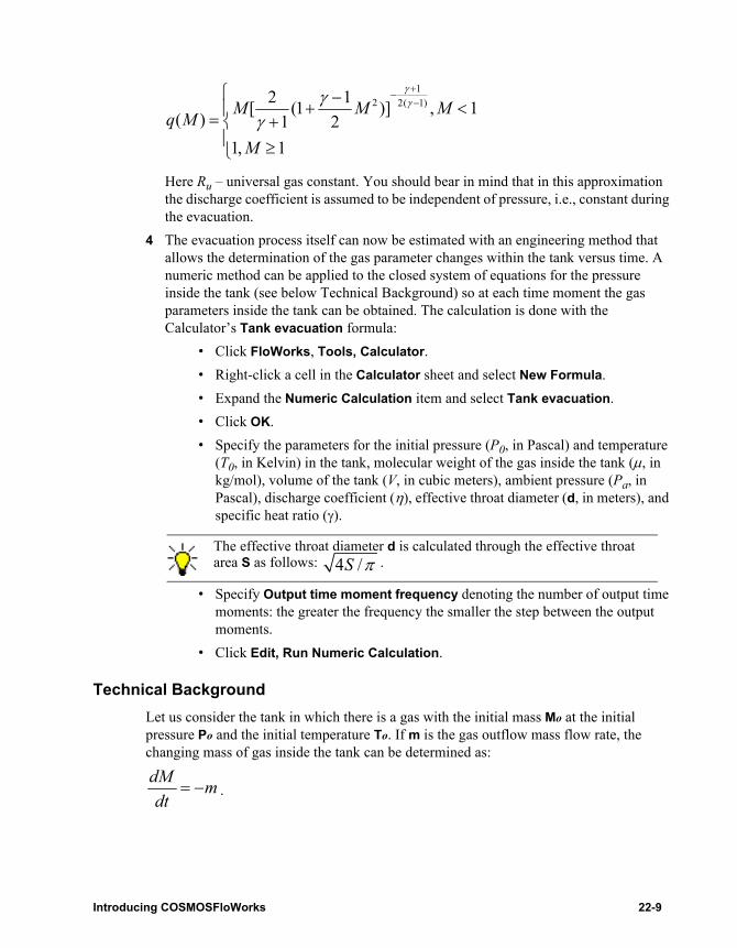
Here Ru – universal gas constant. You should bear in mind that in this approximation the discharge coefficient is assumed to be independent of pressure, i.e., constant during the evacuation.
4 The evacuation process itself can now be estimated with an engineering method that allows the determination of the gas parameter changes within the tank versus time. A numeric method can be applied to the closed system of equations for the pressure inside the tank (see below Technical Background) so at each time moment the gas parameters inside the tank can be obtained. The calculation is done with the Calculator’s Tank evacuation formula:
• Click FloWorks, Tools, Calculator.• Right-click a cell in the Calculator sheet and select New Formula.• Expand the Numeric Calculation item and select Tank evacuation.• Click OK.• Specify the parameters for the initial pressure (P0, in Pascal) and temperature
(T0, in Kelvin) in the tank, molecular weight of the gas inside the tank (µ, in kg/mol), volume of the tank (V, in cubic meters), ambient pressure (Pa, in Pascal), discharge coefficient (η), effective throat diameter (d, in meters), and specific heat ratio (γ).
• Specify Output time moment frequency denoting the number of output time moments: the greater the frequency the smaller the step between the output moments.
• Click Edit, Run Numeric Calculation.
Technical BackgroundLet us consider the tank in which there is a gas with the initial mass Mo at the initial pressure Po and the initial temperature To. If m is the gas outflow mass flow rate, the changing mass of gas inside the tank can be determined as:
.
The effective throat diameter d is calculated through the effective throat area S as follows: .
12 2( 1)2 1[ (1 )] , 1( ) 1 2
1, 1
M M Mq MM
γγγ
γ
+−
− −
+ <= + ≥
4 /S π
dM mdt
= −
Introducing COSMOSFloWorks 22-9
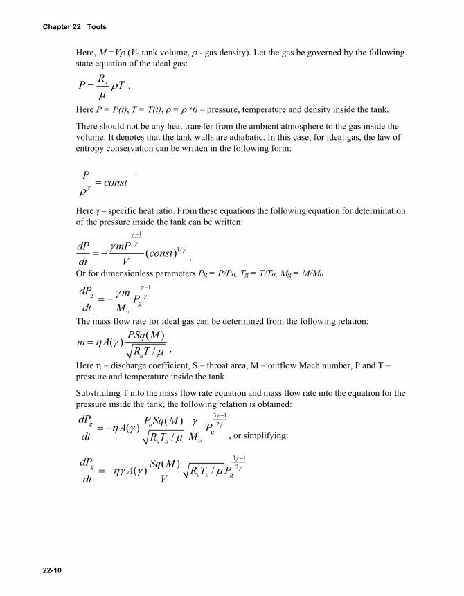
Chapter 22 Tools
Here, M =Vρ (V- tank volume, ρ - gas density). Let the gas be governed by the following state equation of the ideal gas:
.
Here P = P(t), T = T(t), ρ = ρ (t) – pressure, temperature and density inside the tank.
There should not be any heat transfer from the ambient atmosphere to the gas inside the volume. It denotes that the tank walls are adiabatic. In this case, for ideal gas, the law of entropy conservation can be written in the following form:
.
Here γ – specific heat ratio. From these equations the following equation for determination of the pressure inside the tank can be written:
,
Or for dimensionless parameters Pg = P/Po, Tg = T/To, Mg = M/Mo
.
The mass flow rate for ideal gas can be determined from the following relation:
,
Here η – discharge coefficient, S – throat area, M – outflow Mach number, P and T – pressure and temperature inside the tank.
Substituting T into the mass flow rate equation and mass flow rate into the equation for the pressure inside the tank, the following relation is obtained:
, or simplifying:
uRP Tρµ
=
P constγρ=
1
1/( )dP mP constdt V
γγ
γγ−
= −
1g
gv
dP m Pdt M
γγγ −
= −
( )( )/u
PSq Mm AR T
η γµ
=
3 12( )( )
/g o
gou o
dP P Sq MA Pdt MR T
γγγη γ
µ
−
= −
3 12( )( ) /g
u o g
dP Sq MA R T Pdt V
γγηγ γ µ−
= −
22-10

The Much number (M) and q(M) is defined as follows:
Parametric Study
Making a Parametric StudyParametric study is a tool designed to perform a set of calculations varied only by a selected variable parameter (a particular model dimension or a boundary condition parameter) in order to find an analysis (i.e. a specific value of the dimension or parameter of interest) where the selected flow parameter (defined as a goal) will be equal to the specified target value.
The model configurations being different in only variable parameter (dimension or boundary condition parameter) yield different flow field, thus resulting in different goal values for each calculation. The obtained goal value is compared to the target parameter, which can be specified as a constant, table or function dependencies. If the difference between the calculated goal and the parameter is greater than the specified criterion, a new configuration is automatically created with the variable parameter value to be analyzed (the other project settings are maintained the same for every calculation). The secant method is used for choosing the new value. The series of calculations will proceed until the solution is found or the number of calculations has reached the admissible value, or COSMOSFloWorks has detected that no solution can be found in the specified variable parameter range.
For example, you can use the parametric study to obtain a position of a valve's piston so that the force acting on the piston gets balanced to the resistance force of the valve spring. Here, the force acting on the piston should be specified as the force goal and the target parameter is the spring's resistance force specified as a function of dimension.
To make a parametric study:
1 Click FloWorks, Tools, Parametric Study.If you have previously created a parametric study for the current project, click Open and select the .fwps file.
2 The parametric study wizard guides you through the definition of a new study step by step. At the first step, select a type of the parameter to vary:
• Dimension. Varying the dimension value (the dimension is specified on the next step of the wizard), the study will search for the geometry of your model providing the desired value of the selected flow parameter specified as a goal.
12 [( ) 1]1
og
a
PM PP
γγ
γ
−
= −−
12 2( 1)2 1[ (1 )] , 1( ) 1 2
1, 1
M M Mq MM
γγγ
γ
+−
− −
+ <= + ≥
Introducing COSMOSFloWorks 22-11
Chapter 22 Tools
• Flow Parameter. Varying the boundary condition parameter value (the parameter is specified on the next step of the wizard), the study will search for the boundary condition providing the desired value of the selected flow parameter specified as a goal. The variable boundary condition parameters are parameters specified in the General Settings as default parameters (default wall temperature, default wall roughness) or as ambient conditions for external analyses (pressure, density, temperature, velocity), or parameters specified on openings as the Boundary Condition (velocity, mass/volume flow rate, pressure, temperature).
3 Click Next.
Parametric Study - Specifying a Variable Parameter At step 2, specify the study’s variable parameter and the parameter’s definition interval.
To specify a dimension:
1 Make sure the desired dimension is displayed in the graphics area. To show dimensions, in the FeatureManager design tree right-click the Annotations item and select the Display Annotations, Show Feature Dimensions and Show Reference Dimensions items.
2 In the graphics area, select the Dimension you want to vary. To select a distance mate in assemblies, double-click the mate.
3 Specify Minimum and Maximum dimension values, which denote an admissible variation range for the selected dimension.TIP: The computational mesh will be different in each calculation performed in accordance with the model geometry governed by the dimension value. Therefore you should ensure that you would have enough mesh resolution in the region of interest for each calculation, i.e. at any dimension value within the specified range. For that, the local mesh settings can be used. You can also mate the component representing the local region with the dimension dependent component so that the local mesh settings will move together with the component of interest.
4 Click Next.
To specify a boundary condition parameter:
The variable boundary condition parameters are parameters specified in the General Settings as default parameters (default wall temperature, default wall roughness) or as ambient conditions for external analyses (pressure, density, temperature, velocity), or parameters specified on openings as the Boundary Condition (velocity, mass/volume flow rate, pressure, temperature). Note that not all of the parameters are supported for the parametric study; parameters that are not supported are automatically filtered out from the Parameter list.
1 If you want to vary a parameter specified in the General Settings, select it from the Parameter list. To vary a parameter specified as a Boundary Condition, select the
22-12

corresponding boundary condition feature in the COSMOSFloWorks analysis tree, and then select the parameter from the Parameter list. When a boundary condition feature is selected, the General Settings’ are hidden. To remove the feature from the Boundary condition list, select the condition in the list and press the Delete key.
2 Specify the Minimum and Maximum parameter values, which denote an admissible variation range for the selected boundary condition parameter.
3 Click Next.
Parametric Study - Selecting a GoalAt step 3, in the COSMOSFloWorks Analysis tree, select the Goal of interest. The goal value (the average value over the goal's analysis interval) is compared with the target parameter at each calculation after finishing the calculation. The solver will automatically stop the parametric study when the goal value differs from the parameter value by less than the Study convergence criterion specified at Step 4 of the parametric study wizard.
The iterative secant method used requires the first calculations to be performed at the boundaries of the variable interval. The first two calculations are made to obtain the goal value at the min and max variable values. If you know these values or have an approximate estimation, you can direct the study to use these values instead of calculating them, thus reducing the total number of calculations. Click Adjust minimum (maximum) goal value and specify the goal value to be used as a goal minimum (maximum) value.
Click Next.
Parametric Study - Parameter DefinitionAt step 4, specify the parameter value to be compared with the calculated goal value. If the parameter value depends on variable (dimension or boundary condition parameter), you can set this dependence either as a table of values or as a function of the variable. Make sure the specified dependency is monotonic otherwise the correct solution cannot be obtained.
To specify the target parameter:
1 Select the Dependency type either as Constant, Table or Formula:• Constant. The target parameter value is constant throughout the entire variable
range.
Introducing COSMOSFloWorks 22-13

Chapter 22 Tools
• Table. The target parameter value is a function of the variable defined as a linear extrapolation of the table points. In the picture below the parameter dependency is defined using four table points.
To add a new value, click Add Row, double-click the Parameter cell at the right and type the variable parameter value, then double-click the Value cell and type the target parameter value.• Formula. The target parameter value is a function of the variable. To add
variable in the formula, click Add.2 Click Next.
Parametric Study - Finishing ConditionsAt step 5, specify the study's finishing conditions and the way the new calculation is running:
• Study convergence criterion. The calculation stops if the difference between the goal and parameter values is less than the specified Study convergence criterion. This criterion does not affect the convergence and finishing criteria specified for the project in the Calculation Control Options dialog box.
• Specify the Maximum number of calculations to be run.• Specify either to Create a new configuration for each new calculation or make
modification in the current configuration. The new configuration is assigned with the following name: variable = <current_variable_value>.
Click Next.
Parametric Study - CalculationAt the final step, check the summary of the parametric study and click Run to start the study. In the Results box the following information is output for each calculation:
You should carefully inspect the project's finishing conditions. It is recommended that you use the goal of interest for the project's convergence control and set the other finishing conditions so that the calculation will finish with acceptable goal convergence achieved.
22-14

• Iteration. The number of calculation currently running.• Dimension. The dimension value.• Target parameter. The parameter value, which is compared with the goal.• Goal value. The calculation resulting goal value (averaged over the analysis
interval).• Discrepancy. The discrepancy between the goal value and the parameter value.
The study stops due to one of the following reasons:
• Solution is found. The Study convergence criterion was satisfied for the last calculation.
• Solution is not found: the maximum number of calculations is reached. In this case, you most likely need to increase the Maximum number of calculations.
• Solution is not found: the solution cannot be found in the specified variable range. The iterative secant method calculates the next variable value (xi) based on the values obtained at two previous iterations. For the first approach the specified minimum and maximum variable values are used. It is assumed that both the parameter and goal functions are monotonic (monotone decreasing or monotone increasing). So if goal(xmin) < parameter(xmin) and goal(xmax) < parameter(xmax), the solution cannot be obtained because parameter and goal functions do not intersect in the specified variable range. Likewise, if goal(xmin) > parameter(xmin) and goal(xmax) > parameter(xmax). In this case, you most likely need to extend the variable range.
If you click Stop, the parametric study will stop after the current calculation is finished (or you can finish it manually). Note that when you stop the study the study's current state is not saved so the study will run from the beginning (as a new calculation) the next time you click Run.
Simplifying the Model
Allows you to accelerate procedures of meshing and processing results by suppressing fillet features.
Introducing COSMOSFloWorks 22-15

Chapter 22 Tools
If your model has a lot of fillet features, the time, required for operating with the model while creating the computational mesh and processing results dealing with the boundary data, may badly increase due to some Boolean operations performed by COSMOSFloWorks with the model’s bodies (see "Check Geometry" on page 22-16).
If you are sure that some fillets do not act on the flow, or their influence is not substantial, you can suppress the fillets to accelerate procedures of meshing and processing results.
If you do not want to modify your model before the calculation (since you not sure about the fillets influence on the flow) then you can suppress fillets after the calculation has finished to accelerate the processing of results only. Be aware that in this case the displayed and calculated geometry will differ in filleted features.
To automatically suppress fillets of a specified radius:
1 Click FloWorks, Tools, Simplify Model.2 Click Options and specify the Minimum fillet radius so that all fillets with the smaller
radius will be displayed in the list.3 Select a fillet feature to suppress and click Suppress.
– or –Click Suppress All to suppress all existing fillets.
Check Geometry
COSMOSFloWorks divides the SolidWorks model into solid and fluid regions. During certain analyses (i.e. porous media) it may be necessary to convert (Disable) a solid region into a fluid region or suppress the solid region from the analysis entirely. While meshing the model, COSMOSFloWorks first interprets the specified solid and fluid regions as bodies (virtual, in case of fluid) and then creates computational mesh for these bodies. By using the Check Geometry tool you can see these resulting solid and fluid bodies.
This tool also allows you to check the bodies for possible geometry problems (i.e. tangent contact) that cause COSMOSFloWorks to create an inadequate mesh.
To check the model geometry:
1 Click FloWorks, Tools, Check Geometry.2 Specify the project configuration to test. All changes made in the Check Geometry
dialog box have no influence on the current project settings and apply to the tested configuration only:
• For assemblies you can Enable/Disable a component to change its state (fluid or solid) with respect to COSMOSFloWorks. See "Component Control" on page 5-7 for details.
• You can select or clear the Exclude internal space (for external analysis only) and Exclude cavities without flow conditions options. For a definition of these options see "Analysis Type" on page 2-1.
22-16

3 When you click Check, COSMOSFloWorks operates with the model components to get solid and fluid bodies and then calculates the total volume of solids and total fluid volume. Additionally, you can save the resulting solid and/or fluid bodies into assemblies to see exactly the geometry for which the computational mesh will be generated. The created assemblies are saved into the folder specified under the Directory for temporary geometry option in the COSMOSFloWorks Options dialog box. You can also check the resulting bodies for possible invalid contacts. Select the option to check:
• Create solid body assembly. Creates an assembly of solid bodies and saves it in the default folder for temporary geometry.
• Create fluid body assembly. Creates an assembly of fluid bodies and saves it in the default folder for temporary geometry.
• Check for invalid contact. Check the resulting solid and fluid bodies for possible invalid contacts, e.g. tangency, zero thickness, etc. If a problem has been detected, the message appears in the Output box.
4 Click Check. In the Output box you can see the following information:• The fluid volume. For internal analyses this value must not be zero, otherwise
the model is not closed. Internal flow analyses require the model to be fully closed at all openings.
• The solid volume.• The name of the assembly where all solids were saved (if the Create solid body
assembly option s selected).• The name of the assembly where all fluids were saved (if the Create fluid body
assembly option is selected).• In created assemblies there may be some components suppressed. In this case
you will see the names of the suppressed components and the reason why they were suppressed. For example, in assemblies containing fluid bodies of an internal analysis, the external volume is suppressed.
Selection Filter
Allows you to remove unnecessary faces of a specified type from the list of selected faces:
• Remove faces out of the computational domain. When this option is selected, the faces lying out of the Computational Domain are removed from the selection list.
• Remove outer faces (for internal analyses only). When this option is selected, the outer model surfaces are removed from the selection list.
• Remove faces in contact with fluid. When this option is selected, the faces lying on the solid/fluid interface are removed from the selection list. Faces at the solid/porous and fluid/porous interfaces are left in the list.
• Leave only outer faces and faces in contact with fluid. When this option is selected, the only faces at the solid/fluid interface (including the model outer faces
Introducing COSMOSFloWorks 22-17

Chapter 22 Tools
for internal analysis) are left in the selection list. Selecting this option removes from the selection list faces at the solid/solid, solid/porous, porous/fluid interfaces and faces lying out of the computational domain.
22-18

COSMOSFloWorks Toolbars
Click View, Toolbars to access COSMOSFloWorks toolbars.
COSMOSFloWorks Main.
COSMOSFloWorks Features.
COSMOSFloWorks Results Main.
New Project General Settings
Wizard Running Calculation
Clone Project Engineering Database
Global Goal Volume Source
Surface Goal Fan
Volume Goal Local Initial Mesh
Equation Goal Transferred Boundary Conditions
Boundary Conditions Radiative Surface
Initial Conditions Contact Resistance
Porous Medium Fluid Subdomain
Solid Materials Heat Sink Simulation
Surface Source Rotating Region
Load/Unload Results Transient Animation
View Settings Copy image to the Clipboard
Load Time Moment Save the current image
Goal Plot Print Active View
Batch Results Processing
Report
Introducing COSMOSFloWorks 22-19
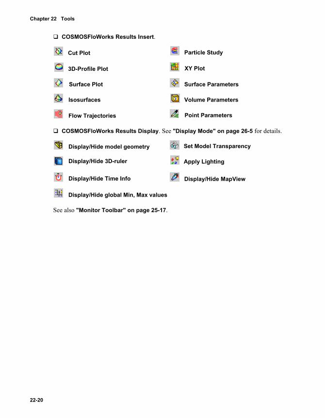
Chapter 22 Tools
COSMOSFloWorks Results Insert.
COSMOSFloWorks Results Display. See "Display Mode" on page 26-5 for details.
See also "Monitor Toolbar" on page 25-17.
Cut Plot Particle Study
3D-Profile Plot XY Plot
Surface Plot Surface Parameters
Isosurfaces Volume Parameters
Flow Trajectories Point Parameters
Display/Hide model geometry Set Model Transparency
Display/Hide 3D-ruler Apply Lighting
Display/Hide Time Info Display/Hide MapView
Display/Hide global Min, Max values
22-20

23 Calculation Control Options
Calculation Control Options - Overview
To access the Calculation Control Options dialog box click FloWorks, Calculation Control Options.
The Calculation Control Options dialog box allows you to specify parameters governing the following COSMOSFloWorks procedures:
making the decision on finishing the calculation. See "Finishing the Calculation" on page 23-2.
invoking refinement of the computational mesh during the calculation. See "Refining Mesh During Calculation" on page 23-3.
saving the results during the calculation. See "Saving Results" on page 23-6.
freezing the flow parameters. See "Advanced Settings" on page 23-7.
(PE ONLY) adjusting the time step for a time-dependent analysis. See "Advanced Settings" on page 23-7.
(PE ONLY) controlling the number of rays traced from the surface if radiating heat transfer is enabled. See "Advanced Settings" on page 23-7.
To set COSMOSFloWorks default values of all these parameters, click Reset. See "Automatic Settings by Reset" on page 23-8.
Introducing COSMOSFloWorks 23-1
Chapter 23 Calculation Control Options
Finishing the Calculation
Using the Finish tab you can specify the conditions of finishing the calculation.
Finish Conditions. In the Value cell select either If one is satisfied, i.e. to automatically finish the calculation as soon as one of the following conditions is satisfied, or If all are satisfied, i.e., to automatically finish the calculation as soon as all of the following conditions are satisfied.
Use the On/Off check box to take into account or abandon the condition when making a decision on finishing the calculation.
The Value cells contain the conditions’ values, which can be specified manually. To manually specify the condition’s value, click the Auto box and select Manual, then double-click the cell at the right and enter the desired value instead of the default value. If you retain the default Auto option, then the condition’s value is specified automatically by COSMOSFloWorks in accordance with the analysis type (internal or external) and the Result resolution level specified in the Wizard or in the Reset box.
You can actuate the following conditions of finishing the calculation:
Minimum refinement number. Regardless of the selected Finish conditions, the calculation cannot finish until the specified number of refinements is performed during the calculation. Thus, even if the If one is satisfied finish condition is selected and there is a condition which is already satisfied, the calculation still continues until the specified number of refinements is performed and the specified Relaxation interval expires after the last refinement. See also "Refining Mesh During Calculation" on page 23-3.
Maximum iterations. The calculation finishes as soon as the specified number of iterations are performed during the calculation.
Maximum physical time (for time-dependent analyses only). The calculation finishes as soon as the specified physical time is reached.
Maximum calculation time. The calculation finishes as soon as the specified maximum CPU time is reached.
Maximum travels. The calculation finishes as soon as the number of travels (flow passages through the computational domain) reaches the specified Maximum travel number.
Goals Convergence. The calculation finishes as soon as the specified goals have converged. If there are no goals specified or no goals are taken into account as finishing conditions, the COSMOSFloWorks internal convergence criteria will be used to finish the calculation.
• Analysis interval (in travels). The interval over which the goals convergence criteria are checked. The analysis interval is reckoned back from the last iteration and indicated by the white bar on the goal plot's X-axis if you select Show analysis interval in the Goal Plot Settings dialog box.
23-2

• Goals Criteria. The goal’s permissible dispersion (in the goal’s units) over the Analysis interval reckoned backward from the current iteration, so, when the goal’s dispersion over this interval becomes lower than this value, the goal is considered as converged. If you clear the On/Off check box for a specific goal, this goal will not influence the task convergence. If you clear the On/Off check box for all specified goals, the task convergence will be only governed by the COSMOSFloWorks internal convergence criteria.
The goals’ dispersions cannot be determined automatically before the calculation, so they are not shown in the Auto mode. The criterion value is seen in the Criterion column of the Goal Plot dialog box.
Refining Mesh During Calculation
Allows you to specify parameters governing the COSMOSFloWorks procedure of adapting the computational mesh to the solution during the calculation. This procedure splits the mesh cells in the high-gradient flow regions, which could not be resolved prior to the calculation or during the previous solution-adaptive mesh refinements, and merges the mesh cells in the low-gradient flow regions. The procedure’s actions are governed by the following parameters specified:
• Refinement level governs the minimum computational mesh cell size, down to which the mesh cells can be split due to the mesh refinement during the calculation with respect to the initial mesh’s cells (see "Initial Mesh - Basic Information" on page 1-8). For example, if the Refinement level equals two, and there are four-level initial mesh cells the solution adaptive refinement can split these cells up to six level cells.
• Refinement Criterion, denoted as εspl, governs the condition of splitting mesh cells during the mesh refinement: if αKspl ≥εspl has been satisfied after the moment specified by the Refinement Strategy, the cell is split into eight daughter cells. Here, α is the neighboring cells coefficient (α=1 in the solid region or if all neighboring cells of the fluid cell lie in the fluid or solid region only) and Kspl is the cell's solution characteristic. The characteristic Kspl is defined as follows:• in the fluid region:
• liquid flows:
Goals are not checked for their convergence criteria until the calculation has past the minimum number of travels (which is 1 travel).
( )∑=
−
∆−
⋅=Nnb
i global
io
io
VVspl T
TTVV
K io
1
4,|||,|max
max rrrr
Introducing COSMOSFloWorks 23-3

Chapter 23 Calculation Control Options
• gas flows, steady-state analyses:
• gas flows, time-dependent analyses:
• in the solid region:
where is the fluid velocity vector, P is the pressure, ρ is the fluid density, T is the temperature, x is the coordinate, Nnb - the number of neighboring cells (from 6 to 24), subscript 0 denotes parameters of the cell under consideration, subscript i denotes parameters of the i-th cell which has a common side with the cell under consideration, subscript sound denotes sound parameters, ∆Tglobal is the temperature difference over the computational domain, j is the j-th coordinate system axis, subscript j(+) denotes parameters of the neighboring cell in the j direction, and subscript j(-) denotes parameters of the neighboring cell in the opposite-to-j direction. All parameters values are taken at the cells centers.• Unrefinement Criterion, let us denote its value as εmer governs the condition of
merging mesh cells during the mesh refinement: if Kmer≤εmer, where Kmer is the eight daughter cells solution characteristic (see its definition below), has been satisfied after each of the iterations performed after the last mesh refinement (or, if the present refinement is the first in the calculation, then after the Start moment of the Periodic Refinement or after its default value of the Tabular Refinement, see below), then the eight daughter cells are merged into the parental cell. Characteristic Kmer is defined in the same manner as Kspl (see above), with the exception of a summation in defining Kmer which is performed over all 36 pairs of the eight daughter cells. Note that the unrefinement criterion merges only cells split by the solution-adaptive refinement.
• Adaptive Refinement in Fluid. When selected, the solution-adaptive refinement is performed within the fluid cells. Uncheck this option to disable the solution-adaptive refinement in fluids.• Use global parameter variation. By default, the cell’s solution characteristic
Kspl is calculated taking into account local parameter variation, e.g., for a cell under consideration, Kspl is calculated only through values from the neighboring cells. This may result in unnecessary refinements invoked in the regions of less
( )∑=
−
−+
−⋅=
Nnb
i io
io
io
io
io
VVspl PP
PPVV
K io
1 ),max(),max(5.0,
|||,|maxmax
ρρρρ
rrrr
( )∑=
−
−+
−⋅=
Nnb
i io
io
io
io
soundisoundisoundosoundo
VVspl PP
PPVV
K iioo
1 ),max(),max(5.0,
|||,|maxmax
ρρρρ
ρρρρ
rrrr
∑=
−+
−
−
+
+
−⋅
−−
−−−
∆=
3
1
)()(
)(
)(
)(
)(
220
j
jj
joj
jo
ojj
oj
globalspl
xxxx
TTxxTT
TK
Vr
23-4

importance. To avoid this, use of global parameter variation is recommended. At that, the corresponding velocity, pressure and density terms are taken relative to the parameter difference over the computational domain:
, , .
Here, the maximum and minimum values are taken over the entire computational domain.
• Adaptive Refinement in Solid. When selected, the solution-adaptive refinement is performed within the solid cells. Uncheck this option to disable the solution-adaptive refinement in solids.
• Approximate Maximum Cells. The solution-adaptive refinement may dramatically increase the number of cells so that the available computer resources (physical RAM) will not be enough for the running calculation. This option allows you to limit the number of cells to the specified Approximate Maximum Cells value. It's possible that the actual mesh count may exceed this maximum cell limit by a small amount to ensure the integrity of the meshed region. Cells with a greater cell’s solution characteristic Kspl are refined first providing optimal refinement in case the maximum cells number is achieved.
• Refinement Strategy governs the calculation moments of refining the computational mesh. You can either retain the Tabular Refinement (used as the default strategy) or select Periodic Refinement or Manual Only refinement.• Units allows you to select units (either travels or iterations) in which the
calculation moments of refining the mesh are measured.• Relaxation interval (in the selected units) is required after the last mesh
refinement before finishing the calculation. The calculation cannot be automatically stopped until the Relaxation interval expires after the last mesh refinement occurred.
• If you have selected Periodic Refinement, you can specify (in the selected units) the Start moment, i.e., the moment of the first refinement, and the Period over which the periodic refinements will be performed.
• If you have selected Tabular Refinement, then, clicking at the Table of refinements cell’s end, you can specify a table of mesh refinement moments (in the selected units) in the corresponding box. See "Table of Refinements" on page 23-6.
• If you have selected Manual Only, the computational mesh will be refined only at the moments of actuating the refinement manually. Note that if you have selected Periodic Refinement or Tabular Refinement, you can perform a manual refinement also.
0
max min
iV VV V
−
−
r r
0
max min
iP PP P
−−
0
max min
iρ ρρ ρ
−−
Introducing COSMOSFloWorks 23-5

Chapter 23 Calculation Control Options
NOTES:
1) The Result resolution level specified in the Wizard or in the Reset dialog box (see "Automatic Settings by Reset" on page 23-8) influences default values of all these parameters.2) If the Refinement and Unrefinement criteria are not satisfied, or the Refinement level is too low, the mesh refinement performed during the calculation is idling, since it does not change the computational mesh.
See also "Solution-Adaptive Meshing - Basic Information" on page 1-10.
Table of Refinements
Allows you to specify moments (in the previously selected units) of refining the computational mesh during the calculation. See "Refining Mesh During Calculation" on page 23-3.
1 Click Add Row, then double click a row and specify the moment in the units shown (travels, iterations, or physical time).
2 If you want to remove a row, select it and click Remove Row(s). To select more than one row, hold down the Shift key while you select.
3 Click OK.
Saving Results
Allows you to specify moments (in selected units) for saving results during the calculation.
Save Before Refinement. If you select this option, the results will be automatically saved during the calculation before each mesh refinement.
Periodic Saving. If you select this option, the results will be periodically saved during the calculation. This option has the following two parameters:
• Units, in which the moments of saving results are specified. You can select either Iterations or Physical time (for time-dependent analyses only)
• Period (in the specified units) of saving the calculation results.
Tabular Saving. If you select this option, the results will be saved at the specified moments during the calculation. This option is specified by Units and Saving Table:
• Units, in which the moments of saving results are specified. You can select either Iterations or Physical time (for time-dependent analyses only).
• Click in the Saving Table cell’s end and in the appearing Table box (see "Table of Savings" on page 23-8) specify a table of moments (in the specified units) of saving the results during the calculation.
23-6

If you solve a time-dependent problem and have specified either Output time step in the Wizard (which can be done in units of physical time only), the specified value (in physical time) appears in the corresponding cell at the present tab (i.e., the Output time step becomes Period of Periodic Saving).
Independently of the selected option, the results are saved into the r_n.fld file, where n is number of the iteration, after which the results are saved.
Advanced Settings
Flow FreezingUnder the Advanced tab you can specify parameters controlling the procedure of saving the CPU time by freezing (i.e., taking from the previous iteration) values of all flow parameters, with the exception of fluid and solid temperatures and fluid substances concentrations (if several substances are considered), which converge more slowly than the other flow parameters, so the temperature and concentrations are calculated at each iteration. This option will be useful when a steady-state or time-dependent problem with substantial heat transfer and/or fluid substances propagation is solved.
To invoke flow freezing, click the Value cell of the Flow Freezing row and select either the Periodic or Permanent strategy for flow freezing.
Periodic flow freezing:• Maximum freezing period (in iterations). If it is equal to N, then the following
procedure will be performed: beginning from the Start moment, the number of sequential iterations with freezing flow parameters after each iteration with their calculation will be increased by one until the N value is reached. Then N sequential iterations with frozen flow parameters are performed after each iteration with their calculation.
• Start moment (in travels) is the calculation moment beginning from which the flow freezing procedure is performed.
Permanent flow freezing denotes freezing the flow parameters beginning from the specified Start moment (in travels), i.e., beginning from this moment the flow parameters, with the exception of fluid and solid temperatures and fluid substance concentrations (if several substances are considered), are not changed in the calculation. As soon as the permanent flow freezing starts, mesh refinements during the calculation are not performed, in spite of the fact that they can be prescribed in the Refinement tab of the Calculation Control Options dialog box.
Manual Time StepIf you solve a time-dependent problem, under the Advanced tab you can specify the problem’s physical time step with which the solution will be marched in time.
Introducing COSMOSFloWorks 23-7

Chapter 23 Calculation Control Options
By default, the time step used for solving time-dependent fluid flow problems is specified by COSMOSFloWorks automatically, based on the fluid flow properties only. If you want either to better resolve a problem’s time-dependent solution (by specifying a smaller time step than the automatically selected one, e.g. for resolving periodic solutions for small periods) or to calculate a heat transfer in solids faster (by specifying a larger time step than the automatically selected one, e.g. if the fluid flow does not change), it is expedient to specify the time step manually. If you solve a time-dependent problem with heat transfer in solids only, i.e., without calculating a fluid flow (the Heat transfer in solids only option is enabled) a manual specification of the time step is preferable.
To specify the time step manually, select the Manual time step check box and double-click the cell at the right of the check box to enter the desired value. If a transient analysis has periods with different characteristic process time, the optimal time step for such analysis should be also dependent on time. The user should decrease the problem’s time step to resolve very quick processes and increase it for the slow processes to speed up the convergence. If you are well aware of such transient processes, you can adjust the manual time step as a formula or table dependency on time.
Radiation View FactorIf you solve a heat transfer analysis with radiation, the View factor resolution level controls the number of rays traced from a surface. It is recommended to increase the View factor resolution level if you have solids with low thermal conductivity.
See also "Calculation Control Options - Overview" on page 23-1.
Table of Savings
Allows you to specify the moments (in the previously selected units) of saving results during the calculation.
1 Click Add Row, then double click a row and specify the moment in the units shown (iterations or physical time).
2 If you want to remove a row, select it and click Remove Row(s). To select more than one row, hold down the Shift key while you select.
3 Click OK.
Automatic Settings by Reset
Using the Reset dialog box you can change the Result resolution level, which governs COSMOSFloWorks automatic values (Auto) of the calculation control options parameters in the Finish and Refinement tabs of the Calculation Control Options dialog box that has been specified in the Wizard. Note that unlike the Result resolution specified in the Wizard, the Result resolution, specified in the Reset dialog box, does not influence the Initial Mesh settings.
23-8

To change the Result resolution level and actuate it:
1 Click Reset in the Calculation Control Options dialog box.2 In the Reset dialog box, select the desired Reset type governing the Calculation
Control Options’ parameters whose values will be automatically changed in accordance with the specified Result resolution level:
• Reset auto fields, if you want the Result resolution level to act only on the parameters’ values specified automatically (Auto),
• Reset all, if you want the Result resolution level to act on values of all parameters at the Finish and Refinement tabs.
• Use the Result resolution level slider to set the desired level.3 Click OK to actuate the specified Result resolution level and return to the Calculation
Control Options dialog box.
Introducing COSMOSFloWorks 23-9

Chapter 23 Calculation Control Options
23-10

24 Solving
Running the Calculation
Starts the calculation for the current project. Use Batch Run if you want to solve a set of projects in a prescribed order.
To calculate the current project:
1 Click Run on the COSMOSFloWorks Main toolbar or FloWorks, Solve, Run.- or -In the COSMOSFloWorks analysis tree, right-click the project name and select Run.
2 Specify how the calculation starts:• Select the New calculation check box if you intend to perform the calculation
from the initial conditions specified in Wizard or General Settings. If you have already performed calculations on the current project and you wish to use a new computational mesh, select the Create mesh check box. Otherwise, the original mesh will be used.
• If you intend to start the new calculation using previous calculation results as an initial condition, select the New calculation, Create mesh, and Take previous results check boxes. For time-dependent analysis, also select a time instant in the Start from time moment list to use results obtained for the instant as an initial condition. This setting does not affect the total analysis time specified in the Wizard’s Time Settings dialog box or in the Calculation Control Options dialog box.
If Run is disabled you may need to rebuild the project. To rebuild, click FloWorks, Project, Rebuild.
If you select the Take previous results option the initial conditions specified in the Wizard or General Settings will be ignored.
Introducing COSMOSFloWorks 24-1
Chapter 24 Solving
If you want to see the complete computational mesh before solver run, select the Create mesh check box only and after mesh generation load the .cpt file. See "Loading Results" on page 26-3.• If you intend to continue the previous calculation select Continue calculation.• You can run the solver on another computer or as a standalone process on the
current computer. Under Run on select the way the solver will be run:• Current Session. The solver will be run on the current computer as a part of
the SolidWorks application (in one process). Use this way if there is enough memory for the calculation (the solver takes about –1.2-1.5 byte per cell). In this case the solver will share the available 2Gb of memory with the SolidWorks application so depending on the model complexity the more memory requested by the SolidWorks application the less memory will be available for the solver.
• If you select the name of the current computer, the solver will be run as a standalone process. For each process there is 2 Gb of memory available, regardless of the amount of physical memory that is actually available. If you run solver as part of the SolidWorks application (Current Session) than the available 2 Gb are shared between the SolidWorks application and the solver resulting in less memory for the calculation. It depends on the model complexity how much memory will be left for the solver calculation. If you run calculation as a standalone process, the total 2Gb will be available for the solver calculation but the total calculation time will be increased compared to the running the solver as part of the SolidWorks application due to the additional data transfer between the SolidWorks application and the solver. The time may greatly increase in cases where solution-adaptive refinements occur during the calculation. Use this way if it is not possible to calculate the task within the current SolidWorks session due to the memory limitation.
• If you select the name of the computer from the local network, the solver will be run on this computer. Click Network Solver to add network computers to the selection list. This way allows you to use the other computer’s CPU and memory resources at the expense of additional calculation time due to data transfer between the network and the current computes.
3 If you want to automatically load the results after the calculation is finished (or if you stop the calculation manually), select the Load results option.
4 For each COSMOSFloWorks project of any currently open model you can define which goal plots, XY-plots, point parameters, surface parameters and volume parameters tables and reports will be automatically created and saved into the project folder after finishing the calculation (or if you stop the calculation manually). Click Batch Results to define the plots, parameter tables and reports to be created. Select Run batch results processing after calculation to create the prescribed plots, parameter tables and reports after calculation. See also "Automatic Results Processing for Set of Calculations" on page 26-7.
5 Click Run.
24-2

Batch Run
Allows you to solve a set of projects in a prescribed order. You can include projects of any currently open document.
To calculate batch of projects:
1 Click FloWorks, Solve, Batch Run.2 To specify projects that you want to calculate, select the corresponding check box in
the Run column.3 For each selected project specify how the calculation starts:
• Select the New calculation check box if you intend to perform the calculation from the initial conditions specified in Wizard or General Settings. If you have already performed calculations of the current project and you wish to use a new computational mesh, select the Create mesh check box. Otherwise, the original mesh will be used.
• If you intend to start the calculation using previous calculation results as an initial condition, select the New calculation, Create mesh, and Take previous results check boxes. For time-dependent analysis, also select a time instant in the Start from time moment list to use results obtained for the instant as an initial condition. This setting does not affect the total analysis time specified in the Wizard’s Time Settings dialog box or in the Calculation Control Options dialog box.
If you want to see the complete computational mesh before solver run, select the Create mesh check box only and after mesh generation load the .cpt file. See "Loading Results" on page 26-3.• If you intend to continue the previous calculation select Continue calculation. • You can run the solver on another computer or as a standalone process on the
current computer. In the Run on column select the way the solver will be run:• Current Session. The solver will run on the current computer as a part of the
SolidWorks application (in one process). Use this method if there is enough memory for the calculation (the solver takes about –1.2-1.5 byte per cell). In this case the solver will share the available 2Gb of memory with the SolidWorks application so depending on the model complexity the more memory requested by the SolidWorks application the less memory that will be available for the solver.
• If you select the name of the current computer, the solver will run as a standalone process. For each process there is 2 Gb of memory available, regardless of the amount of physical memory that is actually available. If you run the solver as part of the SolidWorks application (Current Session) than
If you select the Take previous results option the initial conditions specified in the Wizard or General Settings will be ignored.
Introducing COSMOSFloWorks 24-3

Chapter 24 Solving
the available 2 Gb are shared between the SolidWorks application and the solver resulting in less memory for the calculation. It depends on the model complexity for how much memory will be left for the solver calculation. If you run the calculation as a standalone process, a total of 2Gb will be available for the solver calculation but the total calculation time will be increased compared to running the solver as part of the SolidWorks application due to the additional data transfer between the SolidWorks application and the solver. The time may greatly increase in cases where solution-adaptive refinements occur during the calculation. Use this method if it is not possible to calculate the task within the current SolidWorks session due to the memory limitation.
• If you select the name of the computer from the local network, the solver will be run on this computer. Click Network Solver to add network computers to the selection list. This method allows you to use the other computer’s CPU and memory resources at the expense of additional calculation time due to data transfer between the network and the current computes.
4 For each COSMOSFloWorks project of any currently open model you can define which goal plots, XY-plots, point parameters, surface parameters and volume parameters tables and reports will be automatically created and saved into the project folder after finishing the calculation (or if you stop the calculation manually). Click Batch Results to define the plots, parameter tables and reports to be created. Select the BRP (batch results processing) check box to create the prescribed plots, parameter tables and reports after calculation. See also "Automatic Results Processing for Set of Calculations" on page 26-7.
5 Select the Shutdown monitor check box if you want the solver Monitor dialog box to automatically close after the calculation finishes.
6 Click Up or Down to specify the order of solution of the projects within a document. The project order in the batch is displayed in the Calculation order column.
7 Click Run to start calculations.
You will see the Batch Run dialog box with the changed information in the Status column until all the calculations are completed.
Specifying Computers for Network Solving
Specifies a list of computers from the Local Network on which you can run the calculation.
If some of the selected projects require user's confirmation to make the comprehensive rebuild, such projects will be omitted (indicated by the ‘Canceled’ status) in order not to suspend the batch run calculation.
24-4

To set up a list of computers available for network solving:
1 Specify the computer you want to calculate the task on: • Under Computer name/IP address, type either name or IP address of the computer
from your Local Network and click Add.• Click Browse for Computer and select computer from the local network.• Click Network Search to add to the list all computers from your network (including
the current computer) available for network solving. This procedure may be time consuming since the program traverses all computers in the network and search the appropriate COSMOSFloWorks version installed on them.
• To delete a computer name from the list select the name and click Delete.If COSMOSFloWorks cannot find a solver on the specified network computer which has COSMOSFloWorks installed, you need to check the DCOM settings on that computer.
2 Click OK. You can assign a computer to a particular analysis using the Run on option in the Run or Batch Run dialog boxes.
Introducing COSMOSFloWorks 24-5

Chapter 24 Solving
24-6

25 Monitoring Calculation
Monitoring Calculation - Overview
Allows you to suspend or stop the calculation, manually initiate refinement of the existing computational mesh, change the Calculation Control Options and display the current results during the calculation.
In the Monitor main menu:
Click Calculation, Stop to stop the calculation. You can also hit button to stop the calculation. In both cases you are asked to save the current results or not. If you save results, you will be able to continue the calculation from the saved calculation state. See "Running the Calculation" on page 24-1 for information about how to continue previously stopped calculation.
Click File, Save and Close to stop calculation, save the current results and close the monitor. Click File, Close to stop calculation and close the monitor without saving the current results.
If you want to save the current results, click File, Save Current Results. Results are also automatically saved when the calculation is finished.
Click Calculation, Suspend to suspend or resume the calculation. When checked (the toolbar button is pressed), the calculation is suspended. Although the suspended calculation does not allow you to modify either the SolidWorks model or COSMOSFloWorks project, CPU resources used by COSMOSFloWorks are released.
Click Calculation, Calculation Control Options to open the Calculation Control Options dialog box in order to see or change calculation finishing condition, refining the computational mesh during the calculation, saving the results during the calculation, freezing the flow parameters during the calculation, adjusting the manual time step and controlling number of rays traced from the surface in case the radiating heat transfer is enabled.
Introducing COSMOSFloWorks 25-1

Chapter 25 Monitoring Calculation
Click Calculation, Suspend Options to specify the duration (in minutes) of suspending the calculation.
If you want to manually initiate refinement of the current computational mesh, click Calculation, Refine . Be aware that refinement increases the total calculation time and uses more system resources.
During the calculation you can obtain various information about the calculation process. Click Insert and select one of the following items:
• Log. Displays the history of the current calculation.• Information. Displays mesh statistics and information about the current
calculation step. Also, warns you if improper results can be obtained.• Goal Table. Shows the list of all specified goals, their current value, progress of
convergence, and the goal’s dispersion (Delta) determined over the analysis interval and the goal’s Criterion (see "Finishing the Calculation" on page 23-2). For transient analyses, the parameter increment with respect to the previous iteration (i.e. for the physical time step) is available.
• Preview. Allows you to view the current results on the specified plane. Click Calculation, Update Previews to update preview images if the Auto update option is not selected in the Preview Settings dialog box.
• Goal Plot. For each goal selected in the Add/Remove Goals dialog box, Goal Plot shows the goal convergence diagram, current parameter value, progress of goal convergence, and the goal’s dispersion (Delta) determined over the analysis interval and the goal’s Criterion. For transient analyses, the parameter increment with respect to the previous iteration (i.e., the physical time step back) is available.
• Min/Max Table. Displays the minimum and maximum parameter values at the current iteration calculated over the entire computational domain.
• Refinement Table. Displays information about performed solution-adaptive refinements.
• Summary. Displays the project general settings and input data specified by the user (based on the ID_INPUT_DATA template, see "Creating a Report" on page 26-55 for details).
• Report. Creates a Word document that includes the project general settings and input data specified by the user (based on the ID_INPUT_DATA template).
To easily get a maximized window on top, you can use a window bar at the bottom of the Monitor window. Click View, Window Bar to display the bar. Hold the pointer over a button for a brief time, to display the full name of the corresponding window.
Click View, Status Bar, to display or hide the status bar at the bottom of the Monitor window. This status bar shows the calculation progress.
25-2
Click View, Toolbar to display or hide the Monitor Toolbar that provide quick access to the most frequently used commands.
Click View, Always on Top , if you want to display the Monitor window to always be on top of other windows.
See also "Goals – Basic Information" on page 1-5.
Information and Warnings
To display an Info window, click on the Monitor toolbar or click Insert, Information.
At the top pane, the mesh statistics, current iteration number, the CPU time and the name of the current calculation step are displayed:
• Fluid cells. Number of cells that are in fluid, including partial cells.• Solid cells. Number of cells that are in solid including partial cells (only for heat
transfer analysis). • Iterations. The current iteration number. For time-dependent analyses the number
of iterations is equal to the number of time steps.• Last iteration finished. The time when the last iteration was completed.• Travels. The calculation duration in travels.• Iterations per 1 travel. The number of iterations per 1 travel.• Flow frozen. Displays if the flow freezing is enabled at the current iteration (ON) or
not (OFF).• CPU time. The CPU time expended from the beginning of the calculation to the
current moment.• Physical time. The current physical time for time-dependent analysis.• Calculation time left. The time required to finish the calculation. This value
oscillates during the calculation because it is estimated only approximately.• Status. Displays the current status of the calculation.
The bottom pane displays warning messages if an inaccurate solution is possible:
• The flow has high Mach number, the "High Mach number flow" option is recommended. During a calculation of a gas flow, this message appears if the Mach number value exceeds 3 for steady-state analysis or 1 for transient analysis. If the Mach number greatly exceeds these values we recommend that you stop the calculation and consider the high Mach number gas flows. Otherwise, the solution may be incorrect.
Comment: Maximum Mach number; dV/V - the fluid volume, in which the maximum Mach number value exceeds 3 for steady-state analysis or 1 for transient analysis, divided by the total fluid volume.
Introducing COSMOSFloWorks 25-3
Chapter 25 Monitoring Calculation
To consider the high Mach number gas flows, click FloWorks, General Settings and under the Problem type select the High Mach number flow check box. After changing to high Mach number gas flow, to minimize the time of the new calculation, you can use the previous results as initial conditions by selecting the Take previous results option. See "Running the Calculation" on page 24-1.• The flow has low Mach number, the "High Mach number flow" option is not
recommended. During a calculation of a high Mach number gas flow, this message appears if the maximum Mach number value has become less than 1.5. In this case, the high Mach number flow effects can be neglected. To increase the solution accuracy, we recommend that you stop the calculation and consider the low Mach number gas flows.
Comment: Maximum Mach number.To consider the low Mach number gas flows, click FloWorks, General Settings and under the Problem type clear the High Mach number flow check box. After changing to low Mach number gas flow, to minimize the time of the new calculation, you can use the previous results as initial conditions by selecting the Take previous results option. See "Running the Calculation" on page 24-1.• Supersonic flow is detected within a considerable number of cells. During the
calculation of a low Mach number gas flow, this message appears if the Mach number value exceeds 1 in more than 30% of the cells. In this case the automatic finishing conditions may stop the calculation before it converges so the use of manual stopping criteria is recommended.
• Negative pressure. COSMOSFloWorks has detected negative pressure. Negative pressure may occur at the beginning of the calculation. This does not cause incorrect results. However, if the message appears again, we recommend that you stop the calculation and check the specified condition and general project settings. Otherwise, you may obtain incorrect results.
Comment: Minimum pressure; dV/V - the fluid volume, in which the negative pressure is detected, divided by the total fluid volume.• Solid is melting. Indicates that solid temperature has exceeded a solid Melting
temperature, specified in the Engineering Database.Comment: Material - a solid where the solid melting temperature was exceeded; Max temperature - maximum temperature calculated over the solid; Melting temperature - the value specified in the Engineering Database.• A vortex crosses the pressure opening. During a calculation this message
informs you that there is a vortex crossed by the opening surface at which you specified the pressure Boundary Conditions. In this case the vortex is broken into incoming and outgoing flow components. This may cause incorrect results. A possible solution is to increase the duct length.
Comment: Boundary Condition - name of the pressure boundary condition where the vortex appears; Inlet flow/outlet flow - the ratio of the incoming mass flow rate to the outgoing mass flow rate.
25-4

• Maximum Mach number exceeded. Indicates that somewhere in the fluid the Mach number value has exceeded ten.
Comment: Maximum Mach number; dV/V - the fluid volume, in which the Mach number value exceeds 10, divided by the total fluid volume.• Wrong boundary conditions: mass flow rate is not balanced.
COSMOSFloWorks has detected that specified boundary conditions do not satisfy the law of conservation of mass due to unbalanced mass flow rate. Check to see that total mass flow rate on inlets is equal to total mass flow rate on outlets. Notice that mass flow rate value is recalculated from the velocity or volume flow rate value specified on an opening. To avoid problems with specifying boundary conditions, we recommend that you specify at least one Pressure opening condition since mass flow rate value on Pressure opening is automatically calculated to satisfy the law of conservation of mass.
• Too many cells with small volume. This warning appears if number of partial cells, whose fluid volume is less than one one-hundredth (one percent) of the entire cell's volume, is greater than 25% of all partial cells. This may cause inaccurate results near the model walls resulting in decreasing the overall accuracy. A possible solution is to modify the Computational Domain size or change the initial mesh.
Comment: dN/N - number of partial cells with small fluid volume divided by the total number of partial cells.• Unresolved condition. If you get an Unresolved condition message (Unresolved
fan, Unresolved initial condition, etc.) it means that none of the generated computational mesh cells have this condition applied. For example, if a condition-associated face is not resolved (no cells intersect with the face) by the computational mesh. A possible solution is to modify the generated initial mesh. See "Initial Mesh - Basic Information" on page 1-8.
• Invalid goal. It means that the specified surface or volume goal cannot be calculated correctly because its reference surface or volume (model component) does not have enough information for the goal parameter. This occurs if the surface or volume was not properly resolved during the mesh generation or if the goal parameter is not a valid parameter for the specified surface or volume. For example, you set a force goal on a surface of a component considered as a fluid volume (disabled in Component Control).
• The inlet boundary condition may conflict with the supersonic flow regions. For gas flows using velocity, volume flow or Mach number as an inlet boundary condition, the calculation may be incorrect if the whole flow stream coming from the inlet opening passes through the sonic velocity. The warning informs you in cases of gas analysis with an inlet volume flow, velocity or Mach number condition if somewhere in the computational domain the flow becomes supersonic (Mach ≥ 1). If the results look incorrect (generally indicated by unrealistic pressure or/and density increases), you have to change the inlet boundary condition to a mass flow rate condition.
Comment: Flow opening BC – name of the inlet flow opening condition.
Introducing COSMOSFloWorks 25-5

Chapter 25 Monitoring Calculation
• The achieved pressure ratio exceeds the possible limit, a solution cannot be obtained. This warning appears if the computational pressure exceeds the specified pressure (calculated as average value over all the initial pressure values and the boundary condition pressure values) by a ratio equal to 109. In this case the solution accuracy may decrease. It is recommended to inspect your project’s initial and boundary condition for possible errors in project definition.
• Flow freezing may cause problems. COSMOSFloWorks has detected that enabling the Flow Freezing option may worsen the solution accuracy. If you get this warning it is strongly recommended that you stop the calculation and disable flow freezing.
Comment: Maximum Mach number.• Manual time step has been reduced. COSMOSFloWorks has detected that the
user-defined time step value exceeds the permissible value, which is governed by the flow field and may change during the calculation. In this case, the user-defined value is reduced to the permissible value.
Goal Table
Displays the current status of all goals.
To display a goal table, click on the Monitor toolbars or click Insert, Goal Table.
• Current Value. The current goal value. If no progress bar is displayed for a goal then it means that the goal has no influence on the task convergence.
• Averaged Value, Minimum Value, Maximum Value – the average, minimum and maximum goal values at the goal’s analysis interval.
• Progress. Goal's progress bar is a qualitative and quantitative characteristic of the goal's convergence process. When COSMOSFloWorks analyzes the goal's convergence, it calculates the goal's dispersion defined as the difference between the goal's maximum and minimum values over the analysis interval reckoned from the last iteration and compares this dispersion with the goal's convergence criterion dispersion, either specified by you or automatically determined by COSMOSFloWorks as a fraction of the goal's physical parameter dispersion over the analysis interval reckoned from the fourth iteration until one travel is completed. The percentage of the goal's convergence criterion dispersion to the goal's real dispersion over the analysis interval is shown in the goal's convergence progress bar (when the goal's real dispersion becomes equal or smaller than the goal's convergence criterion dispersion, the progress bar is replaced by word "achieved"). Naturally, if the goal's real dispersion oscillates, the progress bar oscillates. Moreover, when a hard problem is solved, it can noticeably regress, in particular from the "achieved" level. The calculation can finish if the iterations (in travels) required for finishing the calculation have been performed, as well as if the goals' convergence criteria are satisfied before performing the required number of iterations. So, the goal's progress bar together with the goal's plot is useful for
25-6

inspecting the goal's behavior during the calculation, and it does not necessarily indicate when the calculation will finish. If no progress bar is displayed for a goal then it means that the goal’s convergence is not taken into account as a condition of finishing the calculation. See "Finishing the Calculation" on page 23-2.
If you see the Invalid bar, it means that the specified surface or volume goal cannot be calculated correctly because its reference surface or volume (model component) does not have enough information for the goal parameter. This occurs if the surface or volume was not properly resolved during the mesh generation or if the goal parameter is not a valid parameter for the specified surface or volume. For example, you set a force goal on a surface of a component considered as a fluid volume (disabled in Component Control). In other cases, a possible solution is to increase the initial mesh density by increasing the level of initial mesh or decreasing the minimum gap size, minimum wall thickness and by specifying advanced mesh options.• Delta and Criterion. The goal’s dispersion over the analysis interval. The goal is
considered converged if the goal’s dispersion (Delta) over the analysis interval becomes less than the goal’s convergence Criterion determined either by COSMOSFloWorks after beginning of the calculation, or manually specified in the Calculation Control Options dialog box (see "Finishing the Calculation" on page 23-2).
Creating and Editing Goal Plot
To create a goal plot:
1 Click Goal Plot on the Monitor toolbars or click Insert, Goal Plot. The Add/Remove Goals dialog box appears.
2 In the Select goals list, select goals you want to display in the goal plot by selecting checkboxes at the left of each goal’s name.– or –Click Add All to add all project goals to the goal plot.
3 If you want to remove the goal from the goal plot, unselect the checkbox at the left of the goal’s name in the Select goals list.– or –Click Remove All to remove all project goals from the goal plot.
4 In the Plot caption box, type a name for the goal plot.5 Click OK. The goal plot appears.
To edit a goal plot:
1 Right-click any goal row in the top pane of the goal plot window.2 Select Add/Remove Goals to specify goals, which are displayed in the goal plot, and
change the plot name.
Introducing COSMOSFloWorks 25-7

Chapter 25 Monitoring Calculation
Goal Plot
Allows you to observe how parameters, which you specified as goals, are changed during the calculation.
The goal plot window is split into two panes.
Top pane. Displays the current status of the goal. You can control the display of goal plots and edit the current goal plot using the shortcut menu appearing if you right-click the goal row in the top pane of the goal plot window.
To set options for displaying a goal:
1 Right-click the corresponding goal row.2 Select one of the following menu items:
• Show Plot. Displays or hides the goal plot. You can also double-click the goal row to display or hide the goal plot.
• Set Color. Specifies a curve color from the color palette.• Goal Min/Max. Shows minimum, maximum and average goal values within an
abscissa interval. See "Goal Values" on page 25-10.
To edit the current goal plot:
1 Right-click any goal row.2 Select Add/Remove Goals to specify the goals, which are displayed in the goal plot
and change the plot name. See "Creating and Editing Goal Plot" on page 25-7.
Bottom pane. Displays the goal plot.
• To scroll the diagram along the abscissa, click in the graphics area: the cursor is displayed. Hold the mouse button down and drag in the direction you want to scroll.
For lengthy diagrams, it is easiest to use the scroll bar at the bottom.• Right-click in the graphics area to specify Goal Plot Settings.• The white circle on the X-axis indicates the moment of refinement.
Goal Plot Settings
Allows you to specify the display of goal plot.
To set options for displaying goal plots:
1 Right-click in the graphics area of the Goal Plot window: the Goal Plot Settings dialog box appears.
25-8

2 Specify the general goal plot options and numerical settings:
X-axis units. Specifies a coordinate along the horizontal axis (abscissa).• Iterations.Displays the iteration number as abscissa coordinate.• CPU time. The CPU time elapsed from the beginning of the calculation to the
current moment.• Physical time. Physical time for time-dependent analysis.• Travels. Displays travels along the abscissa.
Display value. Specifies which goal value to display as an ordinate parameter.• Current value. The plot ordinate is the current goal value.• Average Value, Maximum Value, Minimum Value. The plot ordinate is the
average, maximum or minimum goal value calculated over the analysis interval reckoned back from the current iteration. Displaying these values can help you better understand the goal behavior due to the lesser influence of the convergence oscillations on these values.
Scale mode. Specifies the general scale mode.• Normalized Scale. Each goal plot is normalized from 0 to 1, so zero corresponds
to the minimum goal value, and one corresponds to the maximum goal value. Both values are taken over the calculation.
• Absolute Scale. Displays all goals in absolute values. Additionally, in this mode, you can apply logarithmic scale to all the plots or manually specify the minimum and maximum values of the ordinate (goal) axis.
Logarithmic scale. In absolute scale mode you can display all goal plots on a logarithmic scale.
Show layout. Displays information about the plot ordinate and abscissa settings.
Show analysis interval. Displays the goals’ analysis interval as a white bar on the X-axis.
Numerical settings. Allows you to display goals within the manually specified range (from Manual min to Manual max) and scale the plot along the X-axis.
• Select the Manual min check box and type the lower-range value of the ordinate (goal) axis.
• Select the Manual max check box and type the upper-range value of the ordinate (goal) axis.
If a goal’s delta is less than the criterion, it is normalized to the 2*Criterion value.
Introducing COSMOSFloWorks 25-9

Chapter 25 Monitoring Calculation
Click Reset Min/Max to show the plot within the actual minimum and maximum values of the ordinate axis.• Plot length. Specifies the plot length so all diagrams are scaled along the X-axis.
This is useful if the plot is too long and scrolling is not practical. Using this slider you can specify the plot scale factor from 0.1 to 10.
• You can also specify the plot length by typing the scale factor value in the Length scale box. The value must be between 0.0001 and 100.
3 Click OK.
See also "Calculation Control Options - Overview" on page 23-1.
Goal Values
Displays the minimum, maximum and average goal value within a specified abscissa interval.This information may be used for estimation of a goal’s convergence.
To display goal values within a specified abscissa interval:
1 Right-click a goal row in the top pane of the Goal Plot window and select Goal Min/Max.
2 In the Goal name list, select a goal whose values you want to display.3 Under Range, with the Min and Max sliders, specify boundaries for the abscissa
interval. This interval is dynamically displayed in the goal plot window. At the top of the window the following parameters are displayed:
• Calculation range. The corresponding minimum and maximum iteration or physical time (for time-dependent analysis).
• Minimum. The minimum goal value within the interval.• Maximum. The maximum goal value within the interval.• Average. The average goal value within the interval.• Delta. The difference between the maximum and minimum values over the
range.
Preview Results
During the calculation run, you can see the current results in a selected plane.
You can also edit minimum/maximum values in place by double-clicking them in the plot area.
25-10

You can create as many previews as you want. If you want to use planes, which are different from the Global Coordinate System planes, you have to create these planes before the calculation starts because you cannot modify the model while the solver is running.
To create a preview:
1 Click Insert Preview on the Monitor toolbar or Insert, Preview: the Preview Settings dialog box appears.
2 In the Preview Settings dialog box, specify the parameters as needed. See "Creating and Editing Preview" on page 25-11.
You can also create a new preview by copying an existing preview. Right-click in the preview window and select Clone, if you want to create a copy of the current preview.
To edit a preview:
1 Right-click in the preview window and select Properties: the Preview Settings dialog box appears.
2 In the Preview Settings dialog box, change the parameters as needed. See "Creating and Editing Preview" on page 25-11.
To save the current preview:
Right-click in the preview window and select Save to File. Browse to the folder where you want to save the image, enter the desired file name and click Save. The image is saved as a standard .bmp file (256 colors).
You can also specify an auto save mode for a preview. See "Preview Options" on page 25-14.
Creating and Editing Preview
To create a preview:
1 Click Insert Preview on the Monitor toolbar or Insert, Preview: the Preview Settings dialog box appears.
2 In the FeatureManager tree, select a plane for displaying results. The selected plane appears in the Plane Name box.
3 Use the arrows or type a value in the Plane offset box to move the plane as desired.4 Under Min/Max mode:
• Selecting Manual min/max allows you to specify a parameter range (Min and Max values on the Settings tab), within which the parameter is shown in the plot. The Manual min/max mode also allows you to specify a Maximum velocity value to control the display of velocity vectors. See "Preview Settings" on page 25-13.
• Click Auto min/max to see the parameter change within its actual range.
Introducing COSMOSFloWorks 25-11
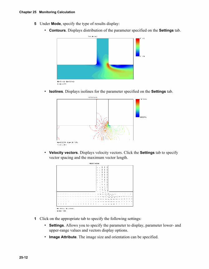
Chapter 25 Monitoring Calculation
5 Under Mode, specify the type of results display:• Contours. Displays distribution of the parameter specified on the Settings tab.
• Isolines. Displays isolines for the parameter specified on the Settings tab.
• Velocity vectors. Displays velocity vectors. Click the Settings tab to specify vector spacing and the maximum vector length.
1 Click on the appropriate tab to specify the following settings:• Settings. Allows you to specify the parameter to display, parameter lower- and
upper-range values and vectors display options.• Image Attribute. The image size and orientation can be specified.
25-12

• Options. Allows you to specify various displaying options: image caption, update mode, the format and step for saving the images, etc.
• Region. Allows you to specify the region for which to display the preview.2 Click OK to accept the changes and close the dialog, or click Apply to update and
proceed with the preview definition.
To edit a preview:
1 Right-click in the preview window and select Properties: the Preview Settings dialog box appears.
2 In the Preview Settings dialog box, change the parameters as needed.
Preview Settings
Allows you to specify a parameter you want to display in the preview plane, the parameter range and display options for velocity vectors.
Contour/Isolines options.
• In the Parameter list select a parameter you want to display in the preview plane.• If you selected Manual min/max on the Definition tab, you can specify lower-range
and upper-range values (Min and Max) to see how a parameter is changing within this range.
Velocity vectors options.
• Maximum velocity. Allows you to control vector display length if Manual min/max option is selected on the Definition tab. Because the vector length is normalized from zero to the Maximum velocity value, you can control the vector length by means of this value. Increase the Maximum velocity value if you want to scale the vectors down in length.
• Vector spacing. Specifies the distance between vector start points.
Introducing COSMOSFloWorks 25-13

Chapter 25 Monitoring Calculation
Preview Image Attributes
Allows you to customize the image size in pixels, and additionally allows you to flip and rotate the image in the preview window.
To specify image size and orientation:
1 Under Image size, select an appropriate size or click User defined and type the custom X-size and Y-size (in pixels). The values must be between 200 and 5000.
2 Under Flip/Rotate image click the option you want.3 Click OK to accept the changes and close the dialog, or click Apply to update and
proceed with the preview definition.
Preview Options
Allows you to specify the image caption, the update mode and the format and step for saving the image. You can also display or hide the intersection of the preview plane with the Computational Domain boundaries and adjust the image size to fit the plane section.
• Auto update. When checked, preview is automatically updated every iteration. Clear this check box if you want to control the preview update. To manually update all previews (that are not auto updated or fixed), click Update All Previews on the Monitor toolbar or Calculation, Update Previews.
If you want to disable the updates for the preview, right-click in the preview window and select Freeze. The preview will not be changed until you deselect the Freeze option.• Auto caption. When checked, the name of the preview window is automatically
generated by COSMOSFloWorks. Clear this check box and type the new window name in the Caption box.
• Auto save. Select this option if you want a preview image to be automatically saved as a standard .bmp file. In this case, you can specify a file name prefix and saving frequency (in iterations).• Auto name prefix. The file name is generated from the prefix and iteration
number (e.g., Pressure (Plane1)_174.bmp).• Auto save step. Allows you to set the iteration frequency for saving the file.By default, the file is saved to the project folder. The project folder is created in the same folder where your SolidWorks model (part or assembly) is located. Click Insert, Summary to get the project output folder path.
You can also manually save the current image. Right-click in the preview window and select Save to File. Browse to the folder where you want to save the image, enter the desired name, and click Save.• Show box. Displays the intersection of the preview plane with the Computational
Domain boundaries.
25-14

• Display mesh. Allows you to display the computational mesh in the preview if the Display mesh option is selected in the General Options dialog box.
Interpolate results. Turns on/off the interpolation of parameter values within cells during preview results visualization. When checked, COSMOSFloWorks displays the distribution of the parameter values so that the calculated values (i.e. values in the mesh cell centers) are interpolated within a cell. Clear this option to turn off the interpolation. In this case the distribution of the parameter values will be constant within a cell.
Preview Region
Specifies the 3D-box that crops the preview area so the preview is only displayed inside the box.
To specify a region the preview is displayed in:
1 Enter a distance from the origin to the corresponding side of the box in the Global Coordinate System. Click Reset to use the entire Computational Domain as a region for displaying the preview.
2 Click OK to create the preview, or click Apply to update and proceed with the preview definition.
Min/Max Table
Displays the minimum and maximum parameter values at the current iteration calculated over the entire computational domain.
To display the Min/Max table:
1 Click Insert, Min/Max Table.2 Adjust the parameters to view: right-click in the min/max table area and choose the
parameters whose minimum and maximum values you want to display. If you want to reset the default set of parameters, click Reset.
Refinement
Refinement means mesh parceling, so the total amount of cells is increased to achieve the specified result resolution. COSMOSFloWorks automatically refines the mesh during the calculation if the specified Result Resolution level is equal to or greater than six. Additionally, for transient tasks refinement may occur to satisfy the internal COSMOSFloWorks convergence criteria.
See also "Solution-Adaptive Meshing - Basic Information" on page 1-10.
Introducing COSMOSFloWorks 25-15

Chapter 25 Monitoring Calculation
Refinement Table
Displays information about the solution-adaptive refinements that occurred during the calculation. The moments of refinement are indicated on the goal plot by the white circle on the X-axis.
To display the refinement information:
1 Click Insert, Refinement Table.2 Under Iterations select an iteration at which the refinement occurred to display the
following refinement information:• Iteration – iteration at which the refinement occurred• Travels – number of travels achieved at the moment of refinement • Physical time – physical time achieved at the moment of refinement (for time-
dependent analyses only)• CPU time – CPU time achieved at the moment of refinement • Maximum allowed level – the maximum level (with respect to the basic mesh
cells) cells can be split is required by the refinement criteria.• History duration – the calculation interval reckoned back from the refinement
moment over which the information about the flow gradients was collected. If the refinement criteria for a cell had been satisfied at least once on the History duration interval, then the cell is split.
• Cells, Fluid Cells, Solid Cells, Partial Cells, Irregular Cells – number of cells before and after the refinement.
You can also display the refinement table after finishing the calculation by clicking FloWorks, Results, Refinement Table.
Suspend Options
Allows you to set the duration of suspending the calculation. By default, the calculation is suspended until you manually continue it.
To set the suspend duration:
1 Click Calculation, Suspend Options.
2 Click Continue calculation in N minutes and specify the Suspend time in minutes.
25-16

Monitor Toolbar
Stops the calculation.
Allows you to suspend or resume the calculation. When button is pressed, the calculation is suspended.
Implements the mesh refinement during the calculation. This option is available if the
specified Result Resolution level is equal to or greater than six or if refinement is enabled in Calculation Control Options.
Updates all preview windows that are not frozen. See "Preview Options" on page 25-14.
Allows the Monitor window to be always on top of other windows.
Displays the history of the calculation.
Displays the Information window.
Displays the Goal Table.
Creates a new Goal Plot.
Creates a new Preview.
Allows you to access the online help system.
Introducing COSMOSFloWorks 25-17

Chapter 25 Monitoring Calculation
25-18

26 Getting Results
Getting Results
After the calculation has finished you can see the flow parameter distribution in various ways. You can display results in all four possible panes of the graphics area. For each pane you can specify different View Settings.Please note that Perspective view is not supported and blocked. To unblock the Perspective view you need to unload COSMOSFloWorks from the Add-Ins.
To get the results:
1 Click FloWorks, Results, Load/Unload Results.– or –In the COSMOSFloWorks analysis tree, right-click the Results icon and select Load Results.
2 In the Load Results box, from the list of files, select the COSMOSFloWorks file containing the results you want to see (a .fld file with the calculation results or a .cpt file with the initial computational mesh only). To decide which of the files contains the required results, see the information about the selected file in the Property/Value list. Rows Iteration and Time (physical) are the most informative for such decisions, especially for time-dependent problems for which several files corresponding to different physical time moments can occur in the list. Click Open to load results from the selected file.The results can be loaded in a quick mode so that only goal plots and report are available to display. Click FloWorks, Results, Select Results and specify the results file (.fld) to load.To unload all results from the memory, click FloWorks, Results, Load/Unload Results again or in the COSMOSFloWorks analysis tree, right-click the Results icon and select Unload Results.
3 Right-click the Mesh icon and select 3D View to see the computational mesh for which the results have been obtained. Select Output to Excel or Output to ASCII if you want
Introducing COSMOSFloWorks 26-1

Chapter 26 Getting Results
to output physical parameters’ values obtained in the selected mesh cells to an Excel or ASCII file. See "Excel Output of Parameters in Cells" on page 26-19 and "ASCII Output of Parameters in Cells" on page 26-19.
4 Click FloWorks, Results, View Settings.– or –In the COSMOSFloWorks analysis tree, right-click the Results icon and select View Settings. You can also right-click in the graphics area and select View Settings.In the View Settings dialog box you specify general display settings and physical parameters to display. These settings and parameters are applied to cut plots, surface plots, flow trajectories and isosurfaces. See "View Settings" on page 26-8 for details.
5 Use the following features to see results:Cut Plot3D Profile Plot
Surface Plots Isosurfaces
Flow Trajectories Particle Study
XY Plot
Surface Parameters
Volume Parameters
Point Parameters Goal Plot
Report
Animation
To show previously created feature, in the COSMOSFloWorks analysis tree, right-click the corresponding feature and select Show.To hide results associated with a particular feature, right-click the corresponding feature and select Hide.To hide results associated with a particular feature and remove graphics data from the memory, right-click the corresponding feature and select Clear and Hide.
6 You can use some additional options for easier displaying of results. Click FloWorks, Results, Display and select the desired mode for the current view. See "Display Mode" on page 26-5.
7 It is possible to copy, save or print the active view. Click FloWorks, Results, Image and select one of the following:
• Copy Image. Copies the active view to the Clipboard.• Save Image. Saves the active view as a .bmp file of the specified size and name. • Print Image. Prints the active view.
26-2

8 You can save the cut plot or surface plot without displaying the plot as an image using the specified format (BMP, JPG, VRML), size and name. See "Customized Saving Images without Visualization" on page 26-53.
Use Results Toolbars that provide quick access to the most frequently used commands.
You can display results in all four possible panes of the SolidWorks graphics area. For each pane you can specify different View Settings.
Click a pane and change the view settings as desired. The active pane is identified by a gray contour around the pane border.
Loading Results
To load result:
1 Click Load/Unload Results on the COSMOSFloWorks Results Main toolbar or click FloWorks, Results, Load/Unload Results.
2 In the Load Results dialog box, from the list of files, select the COSMOSFloWorks file containing the results you want to see:
• .fld file with the calculation results • .cpt file with the initial computational mesh only• r_000000.fld file with the results obtained for the zero iteration, i.e. initial
computational mesh and initial parameters distribution.To decide which of the files contains the required results, see the information about the selected file in the Property/Value list. Rows Iteration and Time (physical) are the most informative for such decisions, especially for time-dependent problems for which several files corresponding to different physical time moments can occur in the list.
3 Click Open to load results from the selected file.
Introducing COSMOSFloWorks 26-3

Chapter 26 Getting Results
Surface Related Parameters
When analyzing the results you can view distributions of different physical parameters (such as pressure, temperature, velocity, heat flux, etc.) on section planes (Cut Plot), on surfaces (Surface Plot), at points (Point Parameters), along lines (XY-Plot), etc. Whatever the case, you must remember that some physical parameters can only be defined on fluid-solid boundaries. These parameters are named surface-related parameters. They are:
• Surface Heat Flux• Shear Stress• Friction Coefficient• Heat Transfer Coefficient• Stanton Number
Fortunately, you do not need to keep in mind all surface-related parameters because COSMOSFloWorks automatically detects if it is possible to display a parameters using the selected tool. For example, COSMOSFloWorks does not allow you to display the surface heat flux in cut plots.
Please note, that the force acting on the selected surface is the sum of the friction and pressure forces acting on the surface and is defined as:
,
where is the friction force and is the pressure force.
,
where is the fluid's shear stress at the wall surface's element of dS area.
,
where P is the calculated static pressure acting on the wall surface's element of dS area and is the reference pressure acting on the wall surface's element of dS area. is a
constant and, therefore, in case of a closed surface:
,
yielding:
,
Pf FFFrrr
+=
fFr
PFr
∫=S
wf SdFrr
τ
wτ
∫∫ ∫ −=−=S
refS S
refP SdPSPdSdPPFrrrr
)(
0== ∫∫S
refS
ref SdPSdPrr
∫=S
P SPdFrr
26-4

Thus you do not have to take into account if the selected surface is closed.
However, if you select the surface which is not closed (e.g. when the symmetry condition is specified or part of the surface is out of the computational domain), the sum of the reference pressure forces acting on the surface is not equal to zero and you have to take them into account when determining the force acting on the surface.
For example, if you calculate the flow over a body (see pictures below) and want to determine the force acting on the flat face of the body in the direction perpendicular to the flow's direction, you should keep in mind that the reference pressure is not compensated because the selected flat surface is not closed and adds to the total force acting on the face. So, in order to determine the value of force acting on the selected face, you need to consider the component of force created by the reference pressure when obtaining the total value of force from COSMOSFloWorks. To do this, you need the value of the reference pressure, which can be found in the Results Summary. (See "Results Summary" on page 26-7).
Display Mode
For conveniently displaying results you can select the various display modes for the active view.
To define a display mode for the active view:
Click FloWorks, Results, Display and select the desired mode:
If all the faces of the body are selected (the whole surface of the body), the total force
created by the reference pressure acting on the surface of the body is equal to zero.
The reference pressure acting on the selected face is not compensated, resulting in the non-
zero value of the reference pressure force (Fref) which adds to the total force acting on the selected surface in the direction of Y axis.
∫∫ +=SS
w SPdSdFrrr
τ
Flow direction Flow direction Fref
Introducing COSMOSFloWorks 26-5

Chapter 26 Getting Results
• Geometry. Displays or hides the model.
• 3D-Ruler. Displays or hides rulers at the computational box. You can set the display options for 3D-Ruler on the Options tab of the View Settings dialog box.
• 2D-Ruler. Displays or hides rulers at the rectangle. You can set the display options for 2D-Ruler on the Options tab of the View Settings dialog box.
• Map View. You can turn on the Map View to see where you are in the model if the model does not fit the graphics area. Once the model is not seen entirely, a half-transparent window appears in the right top corner of the graphics area to show the visible part by the red box or red line intersection. This window disappears as soon as the entire model is visible.
• Time Info. Displays the time instant of the loaded results for a time-dependent analysis.
• Global (Min, Max). For the currently displayed parameter, this option shows the actual minimum and maximum values, calculated over the computational domain. To see how a parameter changes within the specified range, in the View Settings dialog box you can specify parameter minimum and maximum values, which are lower-range and upper-range values. If you select Global (Min, Max), the actual minimum and maximum values are displayed at the top of the graphics area.If you want to see where exactly the maximum and minimum are, you need to create isosurfaces for these values.
• Transparency. Allows you to specify equal transparency for all model components.• Apply Lighting. Turns on the more realistic shaded view of 3D-Profile Plots and
Isosurfaces as well as arrows and spheres along flow and particles trajectories. The lighting properties are acquired from the SolidWorks model's lighting. Note that when the Apply Lighting option is enabled displayed colors change and become different from the color palette selected in the View Settings dialog box.
26-6
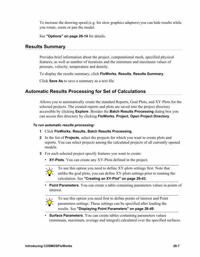
To increase the drawing speed (e.g. for slow graphics adapters) you can hide results while you rotate, zoom or pan the model.
See "Options" on page 26-14 for details.
Results Summary
Provides brief information about the project, computational mesh, specified physical features, as well as number of iterations and the minimum and maximum values of pressure, velocity, temperature and density.
To display the results summary, click FloWorks, Results, Results Summary.
Click Save As to save a summary as a text file.
Automatic Results Processing for Set of Calculations
Allows you to automatically create the standard Reports, Goal Plots, and XY-Plots for the selected projects. The created reports and plots are saved into the project directory accessible by clicking Explore. Besides the Batch Results Processing dialog box you can access this directory by clicking FloWorks, Project, Open Project Directory.
To run automatic results processing:
1 Click FloWorks, Results, Batch Results Processing.2 In the list of Projects, select the projects for which you want to create plots and
reports. You can select projects among the calculated projects of all currently opened models.
3 For each selected project specify features you want to create:• XY-Plots. You can create any XY-Plots defined in the project.
• Point Parameters. You can create a table containing parameters values in points of interest.
• Surface Parameters. You can create tables containing parameters values (minimum, maximum, average and integral) calculated over the specified surfaces.
To use this option you need to define XY-plots settings first. Note that unlike the goal plots, you can define XY-plots settings prior to running the calculation. See "Creating an XY-Plot" on page 26-43.
To use this option you need first to define points of interest and Point parameters settings. These settings can be specified after loading the results. See "Displaying Point Parameters" on page 26-49.
Introducing COSMOSFloWorks 26-7

Chapter 26 Getting Results
• Volume Parameters. You can create tables containing parameters values (minimum, maximum, average, bulk average and integral) calculated within the specified volumes (part or subassembly components in assemblies, as well as bodies in multibody parts) within the Computational Domain.
• Goals. You can create a Goal plot for all project goals.
• Report. You can create reports based on the following standard templates: id_fullreport.dot, id_inputdata.dot, id_results.dot. See "Creating a Report" on page 26-55.
4 Start processing of the results:• Click Run to create the selected plots and reports for the currently highlighted
project. The highlighted project must be checked in the project list to start the batch processing.
• Click Run All to create the selected plots and reports for all projects selected in the project list.
5 Click OK to save settings and close the dialog.
View Settings
In the View Settings dialog box you can specify a physical parameter for the display of contours, isolines, and isosurfaces. You can also control settings for vectors, 3D profile plots, flow trajectories and set advanced display options for the current window or pane. The contours, isolines and vector settings are general for Surface Plots and Cut Plots created in the same window or pane. The contour settings can also be applied for Flow Trajectories, 3D Profile Plots and Isosurfaces. In this case trajectories, 3D profile plots and isosurfaces are colored in accordance with the distribution of the parameter specified on the Contours tab of the View Setting dialog box.
You can access the View Settings dialog box in any of the following ways:
• Click FloWorks, Results, View Settings. • In the COSMOSFloWorks analysis tree, right-click the Results icon and select
View Settings.
To use this option you need first to specify the surfaces and Surface parameters settings. These settings can be specified after loading the results. See "Displaying Surface Parameters" on page 26-46.
To use this option you need first to specify the volumes and Volume parameters settings. These settings can be specified after loading the results. See "Displaying Volume Parameters" on page 26-48.
To use this option you need first to define Goal plot settings. Goal plot settings can be defined after loading results. See "Creating a Goal Plot" on page 26-52.
26-8

• Right-click in the graphics area and select View Settings.• Double-click on the color palette in the graphics area.
The View Settings dialog box has the following tabs:
• Contours. Allows you to specify display settings and the physical parameter for contour plot.
• Isolines. Allows you to specify display settings and the physical parameter of isolines.
• Vectors. Specifies general view settings for vectors used to visualize vector parameters.
• Flow Trajectories. Allows you to specify the way flow trajectories are colored. You can either use a fixed color for all trajectories or apply the contour settings.
• Isosurfaces. Allows you to specify a parameter of isosurfaces and set options for displaying and animating isosurfaces.
• 3D Profile Plot. Allows you to specify a parameter to be displayed as a 3D Profile Plot and the characteristic size of the profile.
• Options. Allows you to specify options for 2D-Ruler, 3D-Ruler, Map View, to control the displaying of the results in the dynamic mode, i.e. while rotating, zooming or panning, and specify the position and the color settings of the palette color bar. See also "Display Mode" on page 26-5.
• Coordinate System. Allows you to select a coordinate system with respect to which the X, Y and Z components of vectors will be displayed in Cut Plots, Surface Plots, Isosurfaces, 3D profile plots and Flow Trajectories.
To customize a list of physical parameters available for display click Parameter List.
ContoursAllows you to set display options for a contour view. In the contour view the entire parameter range is divided by colored intervals so each interval has its own color. You can specify up to 254 colors (intervals). The contour view is applied to cut plots and surface plots so plots display a Parameter distribution in accordance with the specified settings (Min, Max, Palette, and Number of colors). You can also display this parameter on isolines, flow trajectories and isosurfaces if the Use from contours option is selected on the corresponding tab of the View Settings dialog box.
To set display option for a contour view:
1 Click FloWorks, Results, View Settings.2 In the Parameter list, select a parameter for which you want to display contours.3 To see how a parameter changes within the specified range, specify parameter Min and
Max values which are lower-range and upper-range values. Click Reset Min/Max if you want to return the actual minimum and maximum values displayed on the right of the corresponding Min and Max label.
Introducing COSMOSFloWorks 26-9

Chapter 26 Getting Results
TIP: You can change Min and Max values in the graphicsgeometry area. Click a minimum or maximum value on the palette, and type the desired parameter value in the input box. Click to accept the new value or click to cancel changes. You can also change the parameter range by moving corresponding sliders.
4 Select the desired color Palette and specify the Number of colors for the palette. The number of colors is the number of intervals into which the specified parameter range is divided.
5 Click OK to accept the settings and close the dialog box. Click Apply to update and continue to make changes.
TIP: You can easily visualize where a fluid flows against an axis of the Global Coordinate System by displaying the corresponding velocity component in two-color palette with the zero dividing line. This is very convenient for displaying vortices in the flow. For example, to display an area where fluid flows against the X direction, select the X-velocity component in the Parameter list and specify the Number of colors equal to two. Then type any negative value in the Min box and the same positive value in the Max box. The blue color will indicate the area of interest.
IsolinesAllows you to specify a parameter for which you want to display isolines and specify isolines display options. The isolines can be applied for cut plots and surface plots.
To set option for displaying isolines:
1 Click FloWorks, Results, View Settings. The View Settings dialog box appears. Click the Isolines tab.
2 Specify a parameter whose isolines you want to display, the range of parameter changes, and number of isolines.
Click Use from contours if you want to apply the same settings as specified for Contours. In this case, Parameter and the parameter range (Min, Max) are the same as specified on the Contours tab of the View Settings dialog box. The Number of levels is equal to the k = Number of colors+1.Click Use fixed color and, specify the following:
• Parameter. Allows you to specify a parameter for which you want to display isolines. This parameter is displayed if you select Isoline mode for cut plots or surface plots. The parameter color is specified on the Settings tab of the Cut Plot or Surface Plots dialog box.
• To see how a parameter changes within the specified range, specify parameter Min and Max values of this range. Click Reset Min/Max if you want to return
Clicking Reset Min/Max also resets Min and Max values specified for Isolines, 3D Profile and Vectors. To reset contour values only, click the corresponding button.
26-10

the actual minimum and maximum values displayed on the right of the corresponding Min or Max label.
• Number of levels. The specified range (from Min to Max) is divided into k=(Number of levels-1) intervals and isolines are created for all intervals’ bounding values.
3 Click OK to accept the settings and close the dialog box. Click Apply to update and continue to make changes.
VectorsSpecifies display options for vectors. Vectors can be displayed for cut plots and surface plots.
To set display options for vectors:
1 Click FloWorks, Results, View Settings. The View Settings dialog box appears. Click the Vectors tab.
2 Select vector coloring:• Use from contours. Allows you to apply the Contours settings for the vectors.
In this case vectors are colored in accordance with the distribution of parameter specified on the Contours tab. For example, if you want vector color to coincide with the velocity, you must specify Velocity as a parameter on the Contours tab.
• Use fixed color. All vectors have the same color. This color is specified on the Settings tab of the Cut Plot or Surface Plots dialog box.
3 In the Parameter list select a parameter, whose distribution you want to visualize with vectors.
4 To see how the parameter changes within a range, specify the parameter’s Min and Max values of this range. Click Reset Min/Max if you want to return the actual minimum and maximum the parameters values displayed on the right of the corresponding Min or Max label. The vectors whose parameter’s value exceeds the specified Max value will have the same length as the vectors whose parameter’s value is equal to the Max. Likewise, the vectors whose parameter’s value is less than the specified Min value will have the same length as the parameter’s value whose velocity is equal to the Min.
5 Using the slider or typing the Arrow size value in the box, specify the vector size corresponding to the maximum parameter’s value (Max).
6 In the Mode list select the way vectors are displayed:
Clicking Reset Min/Max also resets Min and Max values specified for Contours, 3D Profile and Vectors. To reset values only for contours, click the corresponding button.
Clicking Reset Min/Max also resets Min and Max values specified for Contours, 3D Profile and Isolines. To reset values only for contours, click the corresponding button.
Introducing COSMOSFloWorks 26-11

Chapter 26 Getting Results
• 3D Vectors. Displays spatial vectors.• Projected Vectors. Displays vector projections onto a surface.
7 Click OK to accept the settings and close the dialog box. Click Apply to update and continue to make changes.
Flow TrajectoriesAllows you to specify flow trajectory coloring.
To specify the way flow trajectories are colored:
1 Click FloWorks, Results, View Settings. The View Settings dialog box appears. Click the Flow Trajectories tab.
2 Select flow trajectory coloring:• Click Use from contours if you want flow trajectories to display parameter
specified on the Contours tab of the View Settings dialog box. In this case trajectories are colored in accordance with the distribution of Parameter, parameter range (Min, Max) and the Palette specified on the Contours tab.
• If you click Use fixed color, then no parameter is displayed and all flow trajectories have one color. This color is specified on the Settings tab of the Flow Trajectories dialog box.
3 Click OK to accept the settings and close the dialog box. Click Apply to update and continue to make changes.
IsosurfacesAllows you to specify a display of isosurfaces and create animation of isosurfaces.
Since an isosurface is a surface along which a parameter is constant, it is fully defined by the parameter’s value. No additional inputs are required to display isosurfaces.
To display isosurfaces, right-click the Isosurfaces icon in the COSMOSFloWorks analysis tree and select Show or click FloWorks, Results, Insert, Isosurfaces.
To specify a display of isosurfaces:
1 Click FloWorks, Results, View Settings. The View Settings dialog box appears. Click the Isosurfaces tab.
2 From the Parameter list, select a parameter for which you want to display the isosurfaces. If the Use from contours option is selected, then the Contour parameter defines the isosurface color (see below).
3 Click in the white slider bar to create a slider control that defines an isosurface. You can create up to sixteen isosurfaces.
26-12

Move the slider to specify a parameter value for the isosurface or right-click the slider control and type the desired value in the dialog box, then click OK.
To delete an isosurface, click the slider control and drag it outside the slider area until the pointer appears.
4 Select isosurface coloring:• Click Use from contours if you want isosurfaces to be colored in accordance
with the distribution of the parameter specified on the Contours tab of the View Setting dialog box.
• Click Use fixed color if you want to assign the same fixed color for all isosurfaces. Click Fixed color to select the desired color from the Color palette.
5 Specify the advanced options for displaying isosurface:• Grid. The grid displayed on the isosurfaces helps you to see the geometry of the
isosurface shape. Click Grid to specify the distance between adjacent lines of the grid, which is projected on isosurfaces.
• Region. Allows you to specify the 3D-box that crops isosurfaces so they are only displayed inside the box. In the Region dialog box, enter a distance from the origin to the box sides in the Global Coordinate System. Click Reset to use the entire Computational Domain as a region for displaying isosurfaces.
6 To preview isosurfaces, click the Preview button. Now, changes made for the isosurface definition (changing the parameter, changing the value of parameter, changing the region, etc.) will immediately refresh. All changes made in the Preview mode are not saved until you click Apply or OK.
7 Click OK to accept the settings and close the dialog box. Click Apply to update and continue to make changes.
To create an animation of isosurfaces:
1 Click FloWorks, Results, View Settings. The View Settings dialog box appears. Click the Isosurfaces tab.
2 Specify parameter, color, grid and region as needed, then select the Animation check box.
3 Using the slider, specify the start and finish parameter values for which you want to animate isosurfaces. This range is evenly divided into k = (Number of frames-1) intervals. Isosurfaces will be created for the intervals’ bounding values. If you play the animation, all isosurfaces are displayed in sequence.
4 Click Animate. 5 In the Animation dialog click Create. COSMOSFloWorks creates a standard .avi file
or saves series of bitmap images to create movies in another format. Click Play to run
Introducing COSMOSFloWorks 26-13

Chapter 26 Getting Results
the animation using the default Windows player. Close the Animation dialog to return to the View Settings dialog box.
3D Profile PlotAllows you to specify a parameter which you want to display as a 3D Profile Plot and specify the profile's scale factor.
To set display options for a 3D profile plot:
1 Click FloWorks, Results, View Settings. The View Settings dialog box appears. Click the 3D Profile tab.
2 Specify a parameter you want to display as a 3D profile plot, the range of parameter changes, and the number of levels.• Click Use from contours if you want to apply the same settings as specified for
Contours. In this case, Parameter and the parameter range (Min, Max) are the same as specified on the Contours tab of the View Settings dialog box. The Number of levels is equal to the k = Number of colors+1.
• Click Use fixed color and, specify the following:• Parameter. Allows you to specify a parameter which you want to display as a 3D
Profile plot. The parameter color is specified on the Definition tab of the 3D Profile Plot dialog box.
• To see how a parameter changes within the specified range, specify parameter Min and Max values of this range. Click Reset Min/Max if you want to return the actual minimum and maximum values displayed on the right of the corresponding Min or Max label.
• Number of levels. Defines how accurate the profile's geometry represents the parameter distribution. Increasing the number of levels allows you to represent small parameter gradients by the profile's geometry. Decrease this value if you do not need the detailed representation of the parameter's distribution by the profile.
3 Specify the Distance factor governing how far the point of maximum parameter value is distanced from the reference plane.
4 Click OK to accept the settings and close the dialog box. Click Apply to update and continue to make changes.
OptionsSpecifies the display of 2D-ruler, 3D-ruler and advanced settings for a faster display.
Double-click a Value cell to edit the cell contents or chose the appropriate parameter type.
Clicking Reset Min/Max also resets Min and Max values specified for Contours, 3D Profile and Vectors. To reset values for 3D profile plots only, click the corresponding button.
26-14

2D-Ruler
• Mode. If the Object Fixed mode is selected 2D-Ruler is scaled together with the model. In the Window Fixed mode 2D-Ruler is resized to fit the graphics area.
• Left, Right, Bottom, Top margins. The distance from the graphics area borders to the window fixed 2D-Ruler (in pixels).
• Number of X-ticks, Number of Y-ticks. Controls the number of ticks for the window fixed 2D-Ruler.
• Left, Right, Bottom, Top. The distance from the origin to the sides of the object fixed 2D-Ruler ruler in the Global Coordinate System.
• Grid x-step, Grid y-step. Sets the distance between the adjacent grid lines.• Ruler transparency, Ruler color. Sets color and transparency of the 2D-ruler.• Display grid. Displays or hides the ruler grid.• Grid transparency, Grid color. Sets color and transparency of the grid lines.• Display values. Displays or hides the values at the bottom and right borders of
the 2D-ruler.• Font color, Font transparency, Font size. Specifies font settings for the
displayed values.
3D-RulerBox
• Display while dynamic. Allows you to hide the 3D-Ruler bounding box while the model is being rotated, zoomed or panned. To hide, double-click the Value cell and select No.
• Color. Sets the box color. To change the color, click the Value cell and select the desired color from the color palette.
• Transparency. Sets transparency of the bounding box. To change the transparency, double-lick the Value cell and enter the desired value.
Grid
• Display while dynamic. Allows you to hide the grid while the model is being rotated, zoomed or panned. To hide the grid, double-click the Value cell and select No.
• Xmin, Xmax, Ymin, Ymax, Zmin, Zmax. Lets you specify the box sides on which you want to display grid lines.
• Color. Sets the grid color. To change the color, click the Value cell and select the desired color from the color palette.
• Transparency. Sets transparency of the grid lines. To change the transparency, double-lick the Value cell and enter the desired value.
• x-step, y-step, z-step. Sets the distance between the adjacent grid lines.
Introducing COSMOSFloWorks 26-15
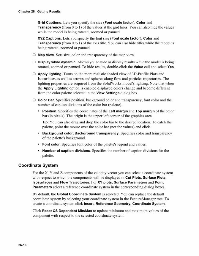
Chapter 26 Getting Results
Grid Captions. Lets you specify the size (Font scale factor), Color and Transparency (from 0 to 1) of the values at the grid lines. You can also hide the values while the model is being rotated, zoomed or panned.XYZ Captions. Lets you specify the font size (Font scale factor), Color and Transparency (from 0 to 1) of the axis title. You can also hide titles while the model is being rotated, zoomed or panned.
Map View. Sets size, color and transparency of the map view.
Display while dynamic. Allows you to hide or display results while the model is being rotated, zoomed or panned. To hide results, double-click the Value cell and select Yes.
Apply lighting. Turns on the more realistic shaded view of 3D-Profile Plots and Isosurfaces as well as arrows and spheres along flow and particles trajectories. The lighting properties are acquired from the SolidWorks model's lighting. Note that when the Apply Lighting option is enabled displayed colors change and become different from the color palette selected in the View Settings dialog box.
Color Bar. Specifies position, background color and transparency, font color and the number of caption divisions of the color bar (palette).• Position. Specifies the coordinates of the Left margin and Top margin of the color
bar (in pixels). The origin is the upper left corner of the graphics area.Tip: You can also drag and drop the color bar to the desired location. To catch the palette, point the mouse over the color bar (not the values) and click.
• Background color, Background transparency. Specifies color and transparency of the palette's background.
• Font color. Specifies font color of the palette's legend and values. • Number of caption divisions. Specifies the number of caption divisions for the
palette.
Coordinate SystemFor the X, Y and Z components of the velocity vector you can select a coordinate system with respect to which the components will be displayed in Cut Plots, Surface Plots, Isosurfaces and Flow Trajectories. For XY plots, Surface Parameters and Point Parameters select a reference coordinate system in the corresponding dialog boxes.
By default, the Global Coordinate System is selected. You can replace the default coordinate system by selecting your coordinate system in the FeatureManager tree. To create a coordinate system click Insert, Reference Geometry, Coordinate System.
Click Reset CS Dependent Min/Max to update minimum and maximum values of the component with respect to the selected coordinate system.
26-16

Plot Manager
Allows you to quickly control the display of the currently available plots. You can also delete the plots even if the results are not loaded.
To control the display of a plot:
1 Click FloWorks, Results, Plot Manager or in the COSMOSFloWorks analysis tree, right-click the Results icon and select Plot Manager. If you want to show/hide plots, you need to load results first. See also "Getting Results" on page 26-1.
2 Select the plot’s row and click the corresponding button to show, hide, clear and hide or delete the selected plot.
3 Click Close.
Parameter List
Allows the selection of parameters to display while viewing results. The enabled parameters appear in the Parameter list of the View Settings dialog box. You can choose parameters from a pre-defined list and/or create your own custom parameters. The custom visualization parameters are defined in the Engineering Database and can be visualized in cut plots, surface plots, isosurfaces, XY-plots and in the point parameters table. See "Specifying Custom Visualization Parameters" on page 22-5.
To enable parameters you want to display:
1 In the View Settings dialog box, click Parameter List.- or - In the analysis tree, right-click the Result icon and select Parameter List.
2 Select parameter you want to display and click Enable.3 Click OK.
For more detailed description of parameters see "List of Parameters and Their Definitions" on page 26-61.
Displaying Refinement Information
Displays information about the solution-adaptive refinements which had occurred during the calculation.
To display the refinement information:
1 Click FloWorks, Results, Refinement Table.2 Under Iterations select the iteration where the refinement occurred to display the
following refinement information:• Iteration – iteration at which the refinement occurred
Introducing COSMOSFloWorks 26-17

Chapter 26 Getting Results
• Travels – number of travels achieved at the moment of refinement • Physical time – physical time achieved at the moment of refinement (for time-
dependent analyses only)• CPU time – CPU time achieved at the moment of refinement • Maximum allowed level – the maximum level (with respect to the basic mesh
cells) cells can be split is required by the refinement criteria.• History duration – the calculation interval reckoned back from the refinement
moment over which the information about the flow gradients was collected. If the refinement criteria for a cell had been satisfied at least once on the History duration interval, then the cell is split.
• Cells, Fluid Cells, Solid Cells, Partial Cells, Irregular Cells – number of cells before and after the refinement.
See also "Solution-Adaptive Meshing - Basic Information" on page 1-10,
"Refining Mesh During Calculation" on page 23-3.
Min/Max Table
Displays the actual minimum and maximum parameter values, calculated over the entire computational domain.
To display the Min/Max table:
Click FloWorks, Results, Min/Max Table
– or –
In the COSMOSFloWorks analysis tree, right-click the Results icon and select Min/Max Table.
Mesh Visualization
Allows you to display the computational mesh cells at the calculation moment selected for getting the results.
To visualize the computational mesh cells:
1 In the COSMOSFloWorks analysis tree, under Results, right-click the Mesh icon and select 3D View to see the computational mesh at which the results have been obtained.
2 In the Cell Options rows, select the types of cells which are of interest (fluid, solid, partial, irregular cells). If you want to see all cells, select All in the Value column. For partial cells you have two additional options: to see partial cells of Small Fluid Volume and to see partial cells of Small Solid Volume. See "Information and Warnings" on page 25-3 for an explanation of such partial cells.
26-18
3 Specify desired colors for showing the cells.4 In the Region rows, specify the computational domain region (through X min, … Z
max), in which the mesh will be shown. To use the full computational domain region, click Reset Region.
5 Click OK.
Excel Output of Parameters in Cells
Allows you to output physical parameter values obtained in the selected mesh cells to an Excel file.
To output physical parameters in cells to an Excel file:
1 In the COSMOSFloWorks analysis tree, under Results, right-click the Mesh icon and select Output to Excel.
2 In the Template row, COSMOSFloWorks offers the Mesh.xlt template to organize data inside an Excel document by default. If you want to use another template, the easiest way to create it is to copy the standard .xlt file and to make changes to the copy in order to ensure that the macro which does the data exchange with COSMOSFloWorks is available. Then place the .xlt file to the <install_dir>\Lang\english\template\Mesh folder to make it available in the Template list.
3 In the Cell Options rows, select the types of cells (fluid, solid, partial, irregular cells) and physical parameters you want to output into the Excel file. To do this, select All in the corresponding Value cells. For partial cells you have two additional options: partial cells of Small Fluid Volume and partial cells of Small Solid Volume. See "Information and Warnings" on page 25-3 for explanation of such partial cells.
4 In the Region rows, specify the computational domain region (through X min, … Z max), from which the mesh cells of the selected type with the physical parameters will be taken. To use the full computational domain region, click Reset Region.
5 In the Parameters rows, select the physical parameters you want to output.6 Select Cell volumes if you want to output the cell volumes and, additionally for partial
cells, the fluid/solid volume ratio for each partial cell (named “Fluid volume part”)7 Click OK.
ASCII Output of Parameters in Cells
Allows you to output physical parameters values obtained in the selected mesh cells to a text (ASCII) file.
To output physical parameters in cells to a text (ASCII) file:
1 In the COSMOSFloWorks analysis tree, under Results, right-click the Mesh icon and select Output to ASCII.
Introducing COSMOSFloWorks 26-19

Chapter 26 Getting Results
2 Specify the file location and name:For a steady-state analysis: in the File row, click the Value cell and in the Save Text File box select the desired folder for saving and type in the file name. By default, the project directory is specified which is accessible by clicking FloWorks, Project, Open Project Directory.For a time-depended analysis:
• In the Directory row, double-click the Value cell and browse for the folder to save the file. By default, the project directory is specified which is accessible by clicking FloWorks, Project, Open Project Directory.
• In the File name template row, specify the file name prefix so the file name is generated from the prefix and the iteration number (e.g., Untitled000010.txt).
3 In the Cell Options rows, select the types of the computational mesh cells (fluid, solid, partial, irregular cells) and physical parameters you want to output into the ASCII file. To do this, select All in the corresponding Value cells. For partial cells you have two additional options: partial cells of Small Fluid Volume and partial cells of Small Solid Volume. See "Information and Warnings" on page 25-3 for explanation of such partial cells.
4 In the Region rows, specify the computational domain region (through X min, … Z max), from which the mesh cells of the selected type will be taken. To use the full computational domain region, click Reset Region.
5 In the Parameters rows, select the physical parameters you want to output.6 Select Cell volumes if you want to output the cell volumes and, additionally for partial
cells, the fluid/solid volume ratio for each partial cell (named “Fluid volume part”).7 For a time-dependent analysis, click Scenario and specify a time moment (or
moments) to output. In the Available results list select a time moment and click Add. To add all available time moments in chronological order, click Reset.
8 Click OK.
Creating a Cut Plot
Cut plot displays a section view of a parameter distribution. The parameter can be represented as a contour plot and as isolines. The physical parameters for contours and isolines are specified in the View Settings dialog box. You can also display velocity vectors in the cut plot.
To create a cut plot:
1 Click FloWorks, Results, Insert, Cut Plot. The Cut Plot dialog box appears.– or –In the COSMOSFloWorks analysis tree, under Results, right-click the Cut Plots icon and select Insert.TIP: If you want to create a copy of the existing cut plot, right click the corresponding cut plot icon and select Clone.
26-20

2 Specify the section plane in which you want to display the results. In the Section plane definition list, select the more convenient way to define the plane:
• Reference. In the FeatureManager tree, select a plane or click a model planar face in which you want to display the results. You can use both standard and reference planes. The only requirement for assemblies is that you must use planes belonging to the top-level assembly.
Use the slider, arrows or type a value in the Section position box to move the plane and change the section cut.• Normal to screen. Allows you to define the section plane normal to the screen.
The plane is specified through two reference points. To specify points, press the mouse button where you want the first point to be, drag to the second point and release the mouse button. You can also type the X and Y coordinates of each point. Coordinates are specified in pixels with respect to the left bottom corner of the graphics area.
• Normal to screen vertical (horizontal). Allows you to define the section plane normal to the screen and vertical (horizontal). To define the plane, click in the graphics area or type the X (Y) coordinate of the reference point. Coordinates are specified in pixels with respect to the left bottom corner of the graphics area.
3 For the Normal to screen (vertical, horizontal) mode, fix the selected section plane:• Click Fix to fix the plane while you rotate, move or pan the model.• Select the Fix at creation time check box, to fix the plane when you press the OK or
Apply button.4 Click View Settings to define the parameter for which you want to display contours
and isolines, as well as general display settings for velocity vectors.
5 For each available medium, specify the way results are displayed. Under Fluid, you specify settings for both gases and liquids. If Heat Conduction in Solids is enabled then temperature can be displayed in solids. You can display solid temperature distribution either with contours or isolines.
• Contours. The cut plot displays distribution of the parameter specified on the Contours tab of the View Settings dialog box.
• Isolines. Displays isolines for the parameter specified on the Isolines tab of the View Settings dialog box. Click the Settings tab to specify isolines display options.
• Vectors. Displays vectors used to visualize vector parameters. Click the Settings tab to specify vector spacing and color. The general display options are specified on the Vectors tab of the View Settings dialog box.
Contour, isoline and vector settings are general for all created result features in the active window or pane. For example, if you change the contour parameter for display using a cut plot, then the same parameter will be displayed for all cut plots, surface plots, isosurfaces, and trajectories, which display contours.
Introducing COSMOSFloWorks 26-21

Chapter 26 Getting Results
• Mesh. Allows you to display the computational mesh in the cut plot if the Display mesh option is selected in the General Options dialog box.
If the Contours or Isolines check box is disabled it means that the specified parameter is not valid. For example you cannot display a contour or isoline plot in solid components unless the specified parameter is temperature in the Contour tab of the View Settings dialog box. Also, you cannot display surface-related parameters in cut plots.
6 Click the Settings tab to specify display options for isolines and velocity vectors used in a cut plot. You can also select options to use the meshed geometry instead of CAD geometry, toggle interpolation of the displayed results, display or hide boundary layer information in the plot and to turn the plot outlines off or on.
7 Click the Region tab to define the 3D box that crops the cut plot.8 To preview the cut plot, click the Preview button at the right of the dialog. Now,
changes made for the plot definition (moving the section plane, adding vectors, changing the region, etc.) will immediately refresh. All changes made in the Preview mode are not saved until you click Apply or OK.
9 Click Save as to save the cut plot as an image of the specified format, size and name without visualization of a plot in the graphics area.
10 Click OK to create the cut plot, or click Apply to update and proceed with the plot definition.
Cut Plot SettingsAllows the selection of display options for isolines and velocity vectors used in a cut plot. You can also select options to use the meshed geometry instead of CAD geometry, toggle interpolation of the displayed results, display or hide boundary layer information in the plot and to turn the plot outlines off or on.
Vectors.
• Vector spacing. Use the slider or type the desired value in the box to control the distance between the vector starting points.
• Uniform plot. Spacing between all vectors is constant.
• Gradient plot. The vector spacing depends on the displayed vector parameter's gradient. The number of vectors is increased in places of higher gradients. That is,
26-22

the more rapidly the vector parameter changes over a given span, the smaller the spacing between the vectors.
• Fixed color. Allows you to define a color of vectors from the Color palette if Use fixed color is selected on the Vectors tab of the View Settings dialog box.
Isolines.
• Fixed color. Allows you to define the isolines’ color from the Color palette if Use fixed color is selected on the Isolines tab of the View Settings dialog box.
• Display values. Displays or hides the parameter values on the isolines.
Background color. Allows you to define a plot background color if contours are not displayed and Draw background check box is selected. To hide contours, click the Definition tab and clear the Contours check box.
Display outlines. Displays or hides the plot area outlines.
Display boundary layer. Displays or hides boundary layers used in the cut plot. Displaying boundary layer requires more computer resources to visualize. Clear this option to increase the creation and operation of the cut plot. When unchecked, the parameter distribution at the boundary layer is ignored (not resolved by the palette).
Use CAD geometry. By default, COSMOSFloWorks shows the original model while displaying results. Depending on how exact the model is resolved by the computational mesh, the original model’s geometry may differ slightly from the geometry on which the calculation is performed. Clear this option to see this COSMOSFloWorks-interpreted geometry instead of the model. See also "Check Geometry" on page 22-16.
Interpolate results. By default, COSMOSFloWorks displays the parameter distribution so that values in the cell’s centers are interpolated within a computational mesh cell. Clear this option to accelerate operations related to displaying results by switching off the interpolation. In this case the cell center parameter data will be displayed without any interpolation between cells.
Cut Plot RegionSpecifies the 3D-box that crops the cut plot area so the plot is only displayed inside the box.
To specify a region the cut plot is displayed in:
1 Enter a distance from the origin to the corresponding side of the box in the Global Coordinate System. Click Reset to use the entire Computational Domain as a region for displaying the cut plot.
Introducing COSMOSFloWorks 26-23

Chapter 26 Getting Results
2 Click OK to create the cut plot, or click Apply to update and proceed with the plot definition.
Animation of Cut PlotsCut plot animation allows you to serially display parallel cut plots having the same display settings as the current one.
To create an animation of the cut plot:
1 Click FloWorks, Results, Insert, Cut Plot. The Cut Plot dialog box appears. – or –In the COSMOSFloWorks analysis tree, under Results, right-click the Cut Plots icon and select Insert.
2 On the Definition, Settings and Region tabs specify display settings for the animated cut plots. Click the Animation tab.
3 Set Number of frames for the animation. Each frame shows a cut plot moved along the cut plane normal within a range specified by Start and finish positions. This range is evenly divided into k = (Number of frames-1) intervals such that cut plots exist at the bounding values.
4 Use the slider to specify Start and finish positions of the cut plane. Right-click the slider control to enter the desired position.
5 Click Animate.6 In the Animation dialog click Create. COSMOSFloWorks creates a standard .avi file
or saves a series of bitmap images to create movies in another format. Click Play to run the animation using the default Windows player. Close the Animation dialog to return to the Cut Plot dialog box.
Creating a 3D Profile Plot
3D Profile Plot displays how a parameter is distributed at the section plane but unlike the cut plot that gives you only color visualization, 3D Plot additionally distances the plot points from the section plane to the distance proportional to the parameter value. The physical parameter and proportionality factor are specified in the View Settings dialog box under the 3D Profile tab.
Temperature Cut Plot Temperature 3D Profile Plot for the same section planes
26-24
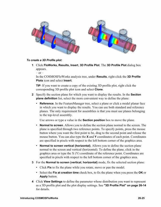
To create a 3D Profile plot:
1 Click FloWorks, Results, Insert, 3D Profile Plot. The 3D Profile Plot dialog box appears.– or –In the COSMOSFloWorks analysis tree, under Results, right-click the 3D Profile Plots icon and select Insert.TIP: If you want to create a copy of the existing 3D profile plot, right click the corresponding 3D profile plot icon and select Clone.
2 Specify the section plane for which you want to display the results. In the Section plane definition list, select the more convenient way to define the plane:• Reference. In the FeatureManager tree, select a plane or click a model planar face
in which you want to display the results. You can use both standard and reference planes. The only requirement for assemblies is that you must use planes belonging to the top-level assembly.Use arrows or type a value in the Section position box to move the plane.
• Normal to screen. Allows you to define the section plane normal to the screen. The plane is specified through two reference points. To specify points, press the mouse button where you want the first point to be, drag to the second point and release the mouse button. You can also type the X and Y coordinates of each point. Coordinates are specified in pixels with respect to the left bottom corner of the graphics area.
• Normal to screen vertical (horizontal). Allows you to define the section plane normal to the screen and vertical (horizontal). To define the plane, click in the graphics area or type the X (Y) coordinate of the reference point. Coordinates are specified in pixels with respect to the left bottom corner of the graphics area.
3 For the Normal to screen (vertical, horizontal) mode, fix the selected section plane:• Click Fix to fix the plane while you rotate, move or pan the model.• Select the Fix at creation time check box, to fix the plane when you press the OK or
Apply button.4 Click View Settings to define the parameter whose distribution you want to represent
as a 3D profile plot and the plot display settings. See "3D Profile Plot" on page 26-14 for details.
Introducing COSMOSFloWorks 26-25

Chapter 26 Getting Results
5 If in the View Settings dialog box you selected the Fixed color for the plot, specify this color and the grid settings. The grid displayed on the 3D profile helps you to see the geometry of the profile shape. Specify Grid step that is the distance between adjacent lines of the grid, which is projected on 3Dprofile.
6 Specify the following display options:• Display outlines. Displays or hides the plot area outlines.• Display boundary layer. Displays or hides boundary layers in the 3D profile plot.
Displaying boundary layer takes more computer resources to visualize. Clear this option for faster creating and operating the plot. When cleared, the parameter distribution at the boundary layer is ignored.
• Use CAD geometry. By default, COSMOSFloWorks shows the original model while displaying results. Depending on how exact the model is resolved by the computational mesh, the original model’s geometry may differ slightly from the geometry on which the calculation is performed. Clear this option to see this COSMOSFloWorks-interpreted geometry instead of the model. See also "Check Geometry" on page 22-16.
7 Click the Region tab to define the 3D box that crops the plot.8 To preview the 3D profile plot, click the Preview button. Now, changes made for the
plot definition (moving the section plane, changing the region, etc.) will immediately refresh. All changes made in the Preview mode are not saved until you click Apply or OK.
9 If you want to change the direction of the 3D profile plot elevation to the opposite one, click Reverse Direction.
10 Click Save as to save the 3D profile plot as an image of the specified format, size and name without visualization of a plot in the graphics area.
11 Click OK to create the 3D profile plot, or click Apply to update and proceed with the plot definition.
3D Profile Plot RegionSpecifies the 3D-box that crops the 3D profile plot area so the plot is only displayed inside the box.
To specify a region the 3D profile plot is displayed in:
1 Enter a distance from the origin to the corresponding side of the box in the Global Coordinate System. Click Reset to use the entire Computational Domain as a region for displaying the cut plot.
2 Click OK to create the 3D profile plot, or click Apply to update and proceed with the plot definition.
26-26
Animation of 3D Profile Plots3D profile plot animation allows you to serially display parallel 3D profile plots having the same display settings as the current one.
To create an animation of the 3D profile plot:
1 Click FloWorks, Results, Insert, 3D Profile Plot. The 3D Profile Plot dialog box appears. – or –In the COSMOSFloWorks analysis tree, under Results, right-click the 3D Profile Plots icon and select Insert.
2 On the Definition and Region tabs specify display settings for the animated 3D profile plots. Click the Animation tab.
3 Set Number of frames for the animation. For a steady-state analysis, each frame shows a 3D profile plot moved along the 3D profile plane normal within a range specified by Start and finish positions. This range is evenly divided into k = (Number of frames-1) intervals such that 3D profile plots exist at the bounding values.
4 Use the sliders to specify Start and finish positions of the 3D profile plane. Right-click the slider control to enter the desired position.
5 Click Animate.6 In the Animation dialog click Create. COSMOSFloWorks creates a standard .avi file
or saves a series of bitmap images to create movies in another format. Click Play to run the animation using the default Windows player. Close the Animation dialog to return to the 3D Profile Plot dialog box.
Creating a Surface Plot
Surface plot displays the parameter distribution on the selected model faces or SolidWorks surfaces. The physical parameters for contours and isolines are specified in the View Settings dialog box. You can also display velocity vectors in the surface plot.
To create a surface plot:
1 Click FloWorks, Results, Insert, Surface Plot.– or –In the COSMOSFloWorks analysis tree, under Results, right-click the Surface Plots icon and select Insert.TIP: If you want to create a copy of the existing surface plot, right click the surface plot icon and select Clone.
2 Select model faces or surfaces on which you want to display a parameter distribution. The selected faces and surfaces are listed in the Surfaces box.– or –
Introducing COSMOSFloWorks 26-27
Chapter 26 Getting Results
Click Use all faces to display parameters on all the faces which are solid-fluid boundaries.
3 Select in which Medium you want to display the parameters if the selected face is the boundary of the different mediums (solid-fluid, fluid-porous or solid-porous). For solids, temperature is the only available parameter to display.
4 Click View Settings to define the parameter for which you want to display contours, parameter for isolines and general display settings for velocity vectors. See "View Settings" on page 26-8 for details.
5 Specify the way results are displayed on the surfaces:• Contours. The surface plot displays the distribution of the parameter specified
on the Contours tab of the View Settings dialog box.• Isolines.Displays isolines for the parameter specified on the Isolines tab of the
View Settings dialog box. Click the Settings tab to specify isolines display options.
• Vectors. Displays vectors used to visualize vector parameters. Click the Settings tab to specify vector spacing and color. The general display options are specified on the Vectors tab of the View Settings dialog box.
• Mesh. Allows you to display the computational mesh in the cut plot if the Display mesh option is selected in the General Options dialog box.
6 Click the Settings tab to specify display options for isolines and velocity vectors of a surface plot. You can also select options to use the meshed geometry instead of CAD geometry, toggle interpolation of the displayed results and to turn the plot outlines off or on.
7 Click the Region tab to define the 3D box that crops the surface plot.8 Click Save as to save the surface plot as an image of the specified format, size and
name without visualization of a plot in the graphics area.9 Click OK to create the surface plot, or click Apply to update and proceed with the plot
definition.
Surface Plot SettingsAllows you set display options for isolines and velocity vectors of a surface plot. You can also select options to use the meshed geometry instead of CAD geometry, toggle interpolation of the displayed results and to turn the plot outlines off or on.
Isolines.
Contour, isoline and vector settings are general for all created result features in the active window or pane. For example, if you change the contour parameter for display using a surface plot, then the same parameter will be displayed for all surface plots, cut plots, isosurfaces, and trajectories which display contours.
26-28

• Fixed color. Allows you to define the isolines color from the Color palette if Use fixed color is selected on the Isolines tab of the View Settings dialog box.
Vectors.
• Fixed color. Allows you to define the vectors color from the Color palette if Use fixed color is selected on the Vectors tab of the View Settings dialog box.
Background color. Allows you to define a plot background color if the contours are not displayed and the Draw background check box is selected. To hide the contours, click the Definition tab and clear the Contours option.
Display outlines. Displays or hides plot area outlines.
Use CAD geometry. By default, COSMOSFloWorks shows the original model while displaying results. Depending on how exact the model is resolved by the computational mesh, the original model’s geometry may differ slightly from the geometry on which the calculation is performed. Clear this option to see this COSMOSFloWorks-interpreted geometry instead of the actual model. See also "Check Geometry" on page 22-16.
Interpolate results. By default, COSMOSFloWorks displays the parameter distribution so that values in the cell’s centers are interpolated within a computational mesh cell. Clear this option to accelerate operations related to the display of results by switching off the interpolation. In this case the cell center parameter data will be displayed without any interpolation between cells.
Surface Plot RegionSpecifies the 3D-box that crops the surface plot area so the plot is displayed only inside the box.
To specify a bounding region for the surface plot:
1 Enter a distance from the origin to the corresponding side of the box in the Global Coordinate System. Click Reset to use the entire Computational Domain as a region for displaying the surface plot.
2 Click OK to create surface plot, or click Apply to update and proceed with the plot definition.
Creating Isosurfaces
You can create up to sixteen isosurfaces of a particular parameter.
To create isosurfaces:
1 Open View Settings dialog box and on the Isosurfaces tab define isosurfaces you want to display.
2 Click FloWorks, Results, Insert, Isosurfaces.– or –
Introducing COSMOSFloWorks 26-29

Chapter 26 Getting Results
In the COSMOSFloWorks analysis tree, under Results, right-click the Isosurfaces icon and select Show.
To hide isosurfaces:
In the COSMOSFloWorks analysis tree, under Results, right-click the Isosurfaces icon and select Hide. In this case all isosurfaces are not visible but still exist and use graphic and memory resources.
To delete isosurfaces:
In the COSMOSFloWorks analysis tree, under Results, right-click the Isosurfaces item and select Clear and Hide.
Displaying Flow Trajectories
Allows you to display flow trajectories as flow streamlines.
Flow streamlines are lines where the flow velocity vector is tangent to that line at any point of the line. To display a streamline specify any streamline point (a point through which the trajectory passes) and the streamline direction with respect to this point. If you specify Forward direction then the streamline is displayed starting from this point. If Backward direction is selected, the streamline is displayed ending at this point. Specifying Both directions allows you to display a flow streamline from the beginning to the end, passing through the selected point.
To display flow trajectories:
1 Click FloWorks, Results, Insert, Flow Trajectories.– or –In the COSMOSFloWorks analysis tree, under Results, right-click the Flow Trajectories icon and select Insert.TIP: If you want to create a copy of the existing flow trajectories feature, right click the corresponding flow trajectories icon and select Clone.
2 In the Start points from list select the way the trajectory points are defined:• Table. Allows you to specify a set of points through which the trajectories pass.
You can either type coordinates of a point or select points on the Reference plane or planar face in the graphics area. These points are displayed on the Table tab of the Flow Trajectories dialog box.
• Reference. The trajectory start points are taken from the selected plane, planar face, sketch, curve or surface.
3 Specify the flow trajectories start points:If Table is selected there are two ways to specify the start points:
• Type the X, Y and Z coordinates of a trajectory start point and click Add.
26-30

• You can pick points from the graphics area:a) Select a plane or planar face whose points are used as trajectory start
points. The only requirement for assemblies is that you must use planes that belong to the top-level assembly. Use the arrows or type a value in the Shift box to move the plane. Orient the plane as desired. We recommend that you use the Normal To view while you select points. Click Fix to make the point selection available.
b) Click in the graphics area to define a point on the plane and click Add. If Auto Add is selected then points are automatically inserted into the Table. The Table contains all trajectories’ points specified. You can also delete points from the Table. See "Flow Trajectories Table" on page 26-33.
• You can copy coordinate values from Excel. Create a table of points in Excel. The x, y and z coordinates must be specified one after another in a row (the same as on the Table tab). Copy the table into the Clipboard, then on the Table tab press Ctrl+V. All points that are inside the computational domain will be inserted into the Table.
If Reference is selected:a) In the SolidWorks FeatureManager Tree select a plane, sketch or curve or
in the graphics area select a planar face or surface. The only requirement for assemblies is that you must use planes, sketches and curves that belong to the top-level assembly. If a plane or a planar face is selected, move the plane to the position you want using the arrows or type a value in the Shift box.
b) Specify the Number of trajectories you want to display.4 In the Direction list, select the direction to display trajectories with respect to the
trajectory start points.5 Click the Settings tab and specify trajectory direction and display options.6 Click View Settings and on the Flow Trajectories tab click Use from contours if you
want trajectories to be colored with the distribution of a parameter specified on the Contours tab of the View Settings dialog box. If you select Use fixed color then all flow trajectories have the same color that you specify on the Settings tab of the Flow Trajectories dialog box.
7 Click the Export tab if you want to see how the parameter value changes along each trajectory you can export the data either into an Excel spreadsheet or a text file.
8 Click Create Curves if you want to create a reference curve feature for each trajectory.9 Click OK to create flow trajectories, or click Apply to update and proceed with
definition of flow trajectories.
Flow Trajectories SettingsAllows you to set flow trajectory spacing and trajectory display options.
• Cross size. Specifies the width of the trajectory band, pipe, arrows and spheres.
Introducing COSMOSFloWorks 26-31

Chapter 26 Getting Results
• Draw trajectories as. The trajectory can be displayed as Line, Band, Line with Arrow or Pipe. Also, discrete Arrows and Spheres can be used to visualize flow trajectories.
• Fixed color. Allows you to define a color of flow trajectories from the Color palette if Use fixed color is selected on the Flow Trajectories tab of the View Settings dialog box.
• Maximum length. Limits the length of the trajectory to the specified value.• Maximum time. Stops the trajectory when the flow traveling time has reached the
specified maximum value.The Maximum length and Maximum time options allow you to save CPU time and computer memory that may be required for processing lengthy trajectories, especially in vortex areas.
• Use CAD geometry. By default, COSMOSFloWorks shows the original model while displaying results. Depending on how exact the model is resolved by the computational mesh, the original model’s geometry may differ slightly from the geometry on which the calculation is performed. Clear this option to see the COSMOSFloWorks-interpreted geometry instead of the actual model. See also "Check Geometry" on page 22-16.
Export Trajectories DataAllows you to export flow trajectory data into an Excel spreadsheet to see how parameters change along each trajectory.
Double-click a Value cell to edit the cell contents or select the appropriate parameter type.
To export trajectories’ data into Excel:
1 Specify a plot abscissa and template for exporting data into Excel:
Abscissa. Allows you to specify the plot abscissa.• Curve Length. Displays parameters against the trajectory length.• Model X, Y, Z. Displays parameters against a coordinate of the Global Coordinate
System.• Time. Displays parameters against the time period during which the fluid goes
along the trajectory.
Template. The flowtrajectories.xlt template is used to organize data inside an Excel document. The easiest way to create a new template is to copy the default flowtrajectories.xlt file and make changes to the copy to ensure that the macro which does the data exchange with COSMOSFloWorks is available. If you are experienced in macro definition, you can modify macros to display data in excel sheets in your own way.Place the .xlt file to the <install_dir>\Lang\english\template\FlowTrajectories folder to make it available in the Template list.
26-32
2 Under Text file path, specify the file name if you wish to output data into a text file.3 Under Fluid Parameters select the parameters whose changes you want to see.4 Click Send to Excel to output data into Excel, or click Send to TXT to output into a
text file.
Flow Trajectories TableDisplays flow trajectory start points that you specified on the Definition tab of the Flow Trajectories dialog box.
You can edit point coordinates directly in the table. To edit point coordinates, double-click the cell and type the desired value.
To delete a point from the table, select the point row and click Delete.
Animation of Flow TrajectoriesAllows you to animate the flow trajectories.
To animate flow trajectories:
1 Click FloWorks, Results, Insert, Flow Trajectories. The Flow Trajectories dialog box appears. – or –In the COSMOSFloWorks analysis tree, under Results, right-click the Flow Trajectories folder and select Insert.
2 On the Definition and Settings tabs define flow trajectories that you want to animate. Then click the Animation tab.
3 Specify Number of frames for the animation. 4 Click Animate.5 In the Animation dialog click Create. COSMOSFloWorks creates a standard .avi file
or saves series of bitmap images to create movies in another format. Click Play to run the animation using the default Windows player. Close the Animation dialog to return to the Flow Trajectories dialog box.
Introducing COSMOSFloWorks 26-33

Chapter 26 Getting Results
Particle Study
Particle study allows you to display trajectories of physical particles and obtain various information about the particle's behavior including their effect on the model walls such as erosion and accumulation. Physical particles are spherical particles of specified material (liquid or solid) and constant mass. Displaying trajectories of physical particles allows you to get knowledge of how extrinsic particles with mass (dust, droplets) are distributed in the flow. These particles do not affect the flow but the flow influences the particle velocity and temperature (resulting in density changes). To study particles you need to specify particles entry points, initial particle properties (temperature, velocity, diameter, produced mass flow rate), particle’s material and the wall condition (absorption or reflection). Optionally, you can enable the gravity and calculate the total accumulation mass rate and the total erosion mass rate.
To make a particle study:
1 Click FloWorks, Results, Insert, Particle Study.– or –In the COSMOSFloWorks analysis tree, under Results, right-click the Particle Study icon and select Insert.
2 On the Injection tab of the Particle Study dialog box, the set of injections specified for the particle study are displayed. Injection is a group of particles of the same material and initial conditions such as velocity, diameter, temperature, etc. When calculating a particle study, an influence of all specified injections is taking into account. • Click Insert and specify an injection. See "Injection" on page 26-35. • Select an injection and click Edit to edit definition of the existing injection. • Select an injection and click Clone to clone the injection.• Select an injection and click Delete to delete the injection.
3 On the Boundary Conditions tab, the specified wall boundary conditions are displayed. The possible wall conditions are absorption, ideal reflection, and non-ideal reflection (considering restitution coefficients). The <Default> condition is applied to all model walls unless it is redefined foe a specific wall. • Select <Default> and click Edit to specify the wall boundary condition by selecting
one of the following types of boundary condition: Absorption, Ideal reflection or Reflection. The selected boundary condition is applied by default for all the models walls.
• Click Insert to customize the wall boundary condition for a specific wall. See "Wall Boundary Condition" on page 26-37.
• Select the condition and click Delete to delete the condition.4 Click the Computational Domain tab if you want to define the calculation region for
the particle study different from the entire computational domain. See "Computational Domain" on page 26-37.
26-34

5 Click Settings and specify the finishing criteria to terminate the calculation of particles trajectories in case the trajectory is too lengthy (for example, in vortex areas). See "Settings" on page 26-38.
6 Click Save Options and specify which fluid and particle parameters you want to output as the particle study results. See "Save Options" on page 26-38.
7 Click Physical models and specify whether to enable gravitation, and to calculate accumulation and erosion of wall material due to particles influence. See "Physical Models" on page 26-39.
8 After you complete the definition of the particle study, click Run to run the calculation or click OK to save the changes and exit the dialog.
9 Once the calculation finishes, right-click the corresponding particle study icon in the analysis tree and select View Results to see the particle study results. See "Particle Study - Results" on page 26-41.
InjectionAllows you to specify injection as a group of particles of the same material and initial conditions such as velocity, diameter, temperature, etc. You can also specify mass flow rate produced by the injection.
To specify an injection:
1 Click Insert in the Particle Study dialog box.– or –Right-click the particle study icon in the analysis tree and select Insert Injection
2 In the Take start points from list select the way the particle start points are defined:• Reference. The specified number of particle start points are evenly taken from the
selected plane or model's surface.• Table. You can either type coordinates of a point or select a point on the Reference
plane or planar face in the graphics area. These points are displayed on the Table tab. You can edit point coordinates directly in the table. To edit point coordinates, double-click the cell and type the desired value. To delete a point from the table, select the point row and click Delete.
• File. You can specify the particles' start points coordinates and initial conditions in a text file, and import this file to define the injection. See "File Format for Injection Definition" on page 26-40 for details.
3 Specify particles' start points:• If Reference is selected:
You can create as many particle studies as you want, but only one study will be active and available for processing. To activate another particle study, right-click the corresponding particle study icon in the analysis tree and select Set as Active Particle Study.
Introducing COSMOSFloWorks 26-35

Chapter 26 Getting Results
a) In the FeatureManager tree select a plane, or in the graphics area select a model surface. If a plane is selected, move the plane to the position you want using the slider or type a value in the Shift box.
b) Specify the number of particles trajectories you want to trace by specifying the corresponding Number of points.
• If Table is selected there are two ways to specify the start points:• Type the X, Y and Z coordinates of a particle start point and click Add.• You can pick points from the graphics area:
a) Select a plane or planar face whose points are used as particle start points. The only requirement for assemblies is that you must use planes that belong to the top-level assembly. Use the slider or type a value in the Shift box to move the plane. Orient the plane as desired. We recommend that you use the Normal To view while you select points. Click Fix to make the point selection available.
b) Click in the graphics area to define a point on the plane and click Add. If Auto Add is selected then points are automatically inserted into the Table. The Table contains all particles’ points specified. You can edit point coordinates directly in the table. To edit point coordinates, double-click the cell and type the desired value. To delete a point from the table, select the point row and click Delete.To turn off the point selection mode, click Fix again.
• If File is selected click Browse to select the file where particles' coordinates and initial conditions are specified.
4 Click the Settings tab and specify initial particle properties (temperature, velocity, and diameter), particles' material and mass flow rate produced by the injection. Double-click a Value cell to edit the cell contents or select the appropriate parameter type.• Initial Conditions.
• Velocity condition type. Allows you to specify the initial particle velocity vector.
• Relative. The particle velocity vector has the same direction as the flow velocity vector at the particle’s start point. The relative Velocity value is a difference between the particle velocity and the flow velocity at the start point. If the relative Velocity value is equal to zero then the flow velocity and initial particle velocity are identical.
• Absolute. The particle velocity vector specified through the X, Y and Z components of the velocity vector with respect to the Global Coordinate System.
• Temperature condition type. Allows you to specify the initial particle temperature either as Absolute or Relative to the fluid temperature at the particle’s entry point. For the Relative type, the negative temperature
26-36

corresponds to the lower temperature of the particles with respect to fluid temperature.
• Temperature. The initial particle temperature. If the Relative type is selected, then zero temperature means that the initial temperature of the particle at the start point is the same as the fluid temperature.
• Diameter. The initial particle diameter. The flow influences the particle temperature and, as a result, the particle density. Since the considered particles are particles of constant mass, the particle volume is variable.
• Mass Flow Rate. Mass flow rate produced by the injection. The value of the mass flow rate defines how many particles fly out in unit time from the opening. The mass flow rate is used to calculate the total erosion/accumulation mass rate. If you use a file to define the injection, the mass flow rate should be specified for each particle's trajectory defining how many particles fly out in unit time from the particle's start point. See also "Physical Models" on page 26-39.
• Particle material. A material (liquid or solid) of the particles. Double-click the cell to select the desired material from the list of materials specified in the Engineering Database.
Wall Boundary ConditionAllows you to specify the particles behavior when they meet a wall. Select one of the following conditions:
• Absorption. The particles are absorbed by the walls. This is typical for liquid particles.
• Ideal reflection. The particles are reflected from the walls. This is typical for solid particles.
• Reflection. Specify the normal en and tangential eτ restitution coefficients which are ratios of the absolute value of the normal and tangential velocity components correspondingly after and before the collision:
Computational DomainAllows you to specify the region where particles are studied. By default the region is the entire computational domain.
n
nn V
Ve
,1
,2=τ
ττ
,1
,2
VV
e =
Introducing COSMOSFloWorks 26-37

Chapter 26 Getting Results
To specify a region where particles are studied:
Enter a distance from the origin to the corresponding side of the box defining the region in the Global Coordinate System. Click Reset to use the entire Computational Domain as a region for the particle study.
SettingsAllows you to specify the finishing criteria to terminate the calculation of particles trajectories. These finishing criteria can be used to save CPU time and computer memory in case of too lengthy trajectories (for example, in vortex areas) and to get the additional knowledge of the trajectory behavior by tracing the trajectories step by step.
Each trajectory is formed step by step by prolonging the trajectory from one point to another on a distance defined as the local velocity at the first point multiplied by the time step defined automatically by the program. Here, one iteration means one step to move from point to point.
• Maximum iteration count. The maximum number of iterations passed. By default the maximum iteration count is specified large enough to avoid terminating the trajectory by this criteria. Decrease the maximum iteration count if only you want to get more details by tracing the trajectories step by step.
• Maximum length. Limits the length of the particle's trajectory to the specified value.
• Maximum time. Stops the particle's trajectory when the particle traveling time has reached the specified maximum value.
• Use CAD geometry. By default, COSMOSFloWorks uses the original model while creating the trajectories. Depending on how exact the model is resolved by the computational mesh, the original model’s geometry may differ slightly from the geometry on which the calculation is performed. Clear this option to calculate the particles trajectories using the COSMOSFloWorks-interpreted geometry instead of the original model. See also "Check Geometry" on page 22-16.
Save OptionsAllows you to specify parameters you want to be available for results processing after the calculation of the particle study. Optionally, you can save the output parameter values to a text file automatically after finishing the calculation of the particle study.
In the Parameter list select which parameters you want to be available the particle study results processing:
• Fluid Parameters. All fluid parameters are always available for processing the particle study results. The selected fluid parameters are saved into the results file that accelerates processing of the particle study results when fluid parameters are output.
26-38
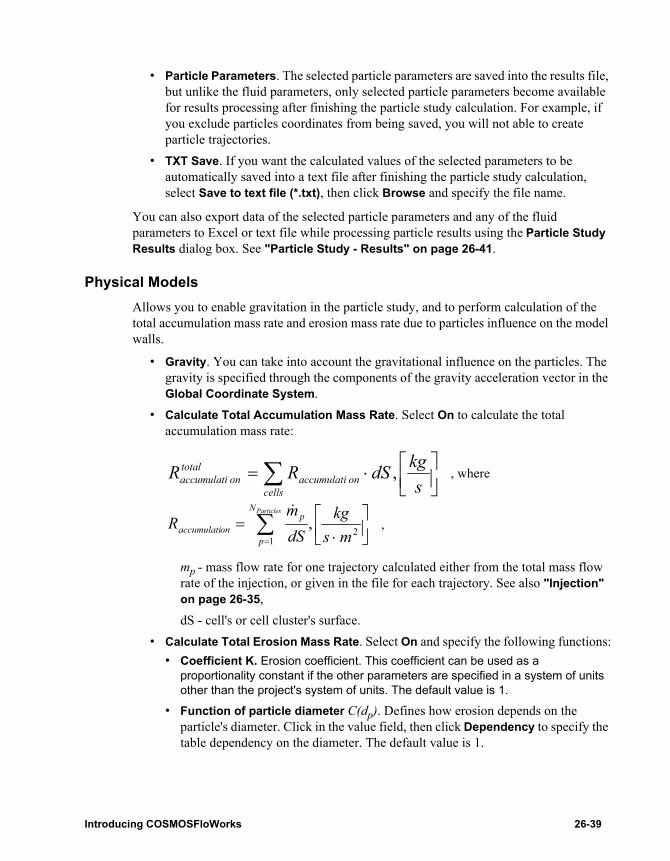
• Particle Parameters. The selected particle parameters are saved into the results file, but unlike the fluid parameters, only selected particle parameters become available for results processing after finishing the particle study calculation. For example, if you exclude particles coordinates from being saved, you will not able to create particle trajectories.
• TXT Save. If you want the calculated values of the selected parameters to be automatically saved into a text file after finishing the particle study calculation, select Save to text file (*.txt), then click Browse and specify the file name.
You can also export data of the selected particle parameters and any of the fluid parameters to Excel or text file while processing particle results using the Particle Study Results dialog box. See "Particle Study - Results" on page 26-41.
Physical ModelsAllows you to enable gravitation in the particle study, and to perform calculation of the total accumulation mass rate and erosion mass rate due to particles influence on the model walls.
• Gravity. You can take into account the gravitational influence on the particles. The gravity is specified through the components of the gravity acceleration vector in the Global Coordinate System.
• Calculate Total Accumulation Mass Rate. Select On to calculate the total accumulation mass rate:
, where
,
mp - mass flow rate for one trajectory calculated either from the total mass flow rate of the injection, or given in the file for each trajectory. See also "Injection" on page 26-35,dS - cell's or cell cluster's surface.
• Calculate Total Erosion Mass Rate. Select On and specify the following functions:• Coefficient K. Erosion coefficient. This coefficient can be used as a
proportionality constant if the other parameters are specified in a system of units other than the project's system of units. The default value is 1.
• Function of particle diameter C(dp). Defines how erosion depends on the particle's diameter. Click in the value field, then click Dependency to specify the table dependency on the diameter. The default value is 1.
∑
⋅=
cellsonaccumulati
totalonaccumulati s
kgdSRR ,
⋅= ∑
=2
1
,ms
kgdSm
RParticlesN
p
ponaccumulati
&
Introducing COSMOSFloWorks 26-39
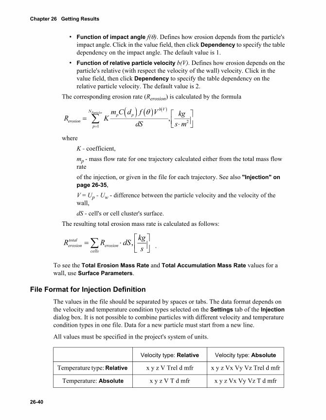
Chapter 26 Getting Results
• Function of impact angle f(θ). Defines how erosion depends from the particle's impact angle. Click in the value field, then click Dependency to specify the table dependency on the impact angle. The default value is 1.
• Function of relative particle velocity b(V). Defines how erosion depends on the particle's relative (with respect the velocity of the wall) velocity. Click in the value field, then click Dependency to specify the table dependency on the relative particle velocity. The default value is 2.
The corresponding erosion rate (Rerosion) is calculated by the formula
whereK - coefficient,mp - mass flow rate for one trajectory calculated either from the total mass flow rateof the injection, or given in the file for each trajectory. See also "Injection" on page 26-35,V = Up - Uw - difference between the particle velocity and the velocity of the wall,dS - cell's or cell cluster's surface.
The resulting total erosion mass rate is calculated as follows:
.
To see the Total Erosion Mass Rate and Total Accumulation Mass Rate values for a wall, use Surface Parameters.
File Format for Injection DefinitionThe values in the file should be separated by spaces or tabs. The data format depends on the velocity and temperature condition types selected on the Settings tab of the Injection dialog box. It is not possible to combine particles with different velocity and temperature condition types in one file. Data for a new particle must start from a new line.
All values must be specified in the project's system of units.
Velocity type: Relative Velocity type: Absolute
Temperature type: Relative x y z V Trel d mfr x y z Vx Vy Vz Trel d mfr
Temperature: Absolute x y z V T d mfr x y z Vx Vy Vz T d mfr
( ) ( ) ( )
21
,Particles
b VNp p
erosionp
m C d f V kgR KdS s m
θ
=
= ⋅ ∑
⋅= ∑ skgdSRR
cellserosion
totalerosion ,
26-40
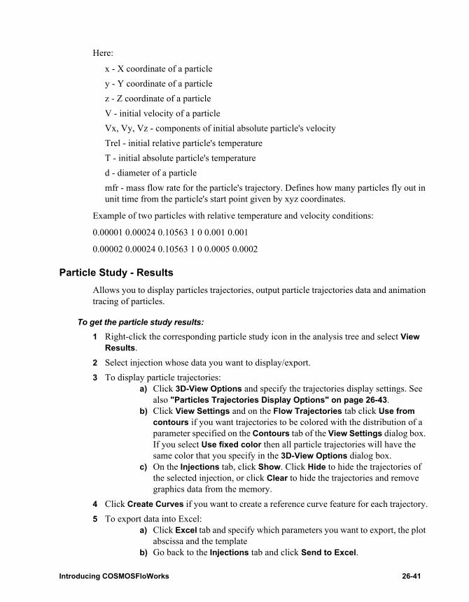
Here:
x - X coordinate of a particley - Y coordinate of a particlez - Z coordinate of a particleV - initial velocity of a particleVx, Vy, Vz - components of initial absolute particle's velocityTrel - initial relative particle's temperatureT - initial absolute particle's temperatured - diameter of a particlemfr - mass flow rate for the particle's trajectory. Defines how many particles fly out in unit time from the particle's start point given by xyz coordinates.
Example of two particles with relative temperature and velocity conditions:
0.00001 0.00024 0.10563 1 0 0.001 0.001
0.00002 0.00024 0.10563 1 0 0.0005 0.0002
Particle Study - ResultsAllows you to display particles trajectories, output particle trajectories data and animation tracing of particles.
To get the particle study results:
1 Right-click the corresponding particle study icon in the analysis tree and select View Results.
2 Select injection whose data you want to display/export.3 To display particle trajectories:
a) Click 3D-View Options and specify the trajectories display settings. See also "Particles Trajectories Display Options" on page 26-43.
b) Click View Settings and on the Flow Trajectories tab click Use from contours if you want trajectories to be colored with the distribution of a parameter specified on the Contours tab of the View Settings dialog box. If you select Use fixed color then all particle trajectories will have the same color that you specify in the 3D-View Options dialog box.
c) On the Injections tab, click Show. Click Hide to hide the trajectories of the selected injection, or click Clear to hide the trajectories and remove graphics data from the memory.
4 Click Create Curves if you want to create a reference curve feature for each trajectory.5 To export data into Excel:
a) Click Excel tab and specify which parameters you want to export, the plot abscissa and the template
b) Go back to the Injections tab and click Send to Excel.
Introducing COSMOSFloWorks 26-41

Chapter 26 Getting Results
6 To export data into a text file:a) Click Excel tab and specify which parameters you want to export.b) Go back to the Injections tab and click Send to TXTc) Specify the file name and click Save.
7 Click Summary to display information about the particle start points, trajectories length, residence time and how a particle finishes its life. See "Particles Tracing Summary" on page 26-42.
8 Click OK to exit the dialog.
Exporting into ExcelAllows you to export particle trajectories data into an Excel spreadsheet to see how parameters change along each trajectory.
Click a Value cell to edit the cell contents or select the appropriate parameter type.
To export trajectories’ data into Excel:
1 Specify a plot abscissa and template for exporting data into Excel:• Abscissa. Allows you to specify the plot abscissa.• Template. The flowtrajectories.xlt template is used to organize data inside an
Excel document. The easiest way to create a new template is to copy the default flowtrajectories.xlt file and make changes to the copy to ensure that the macro which does the data exchange with COSMOSFloWorks will be available in the new template. If you are experienced in macro definition, you can modify macros to display data in excel sheets in your own way.Place the .xlt file to the <install_dir>/Lang/english/template/FlowTrajectories folder to make it available in the Template list.
2 Under Fluid Parameters and/or Particle Parameters select the parameters whose changes you want to see. Please note that the available particle parameters are parameters which you have selected to save when defining the particle study. See "Save Options" on page 26-38.
3 On the Injections tab, select the injection and click Send to Excel.
Particles Tracing SummaryDisplay information about the particle start points, trajectories length, residence time and how a particle finishes its life.
• Trajectories. Display particle start points for all injections in the study.• Length. Trajectory length.• Residence time. The "life time" of a particle. Displays how long the particle exists
within the calculated domain.• Fate. Displays how the particle finishes its life. The possible variants are:
• Opening. The particle reached an opening (flied out the model).
26-42
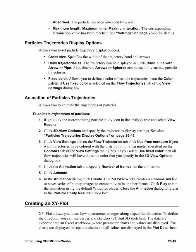
• Absorbed. The particle has been absorbed by a wall.• Maximum length, Maximum time, Maximum iteration. The corresponding
termination value has been reached. See "Settings" on page 26-38 for details.
Particles Trajectories Display OptionsAllows you to set particle trajectory display options.
• Cross size. Specifies the width of the trajectory band and arrows.• Draw trajectories as. The trajectory can be displayed as Line, Band, Line with
Arrow or Pipe. Also, discrete Arrows or Spheres can be used to visualize particle trajectories.
• Fixed color. Allows you to define a color of particle trajectories from the Color palette if Use fixed color is selected on the Flow Trajectories tab of the View Settings dialog box.
Animation of Particles TrajectoriesAllows you to animate the trajectories of particles.
To animate trajectories of particles:
1 Right-click the corresponding particle study icon in the analysis tree and select View Results.
2 Click 3D-View Options and specify the trajectories display settings. See also "Particles Trajectories Display Options" on page 26-43.
3 Click View Settings and on the Flow Trajectories tab click Use from contours if you want trajectories to be colored with the distribution of a parameter specified on the Contours tab of the View Settings dialog box. If you select Use fixed color then all flow trajectories will have the same color that you specify in the 3D-View Options dialog box.
4 Click the Animation tab and specify Number of frames for the animation. 5 Click Animate.6 In the Animation dialog click Create. COSMOSFloWorks creates a standard .avi file
or saves series of bitmap images to create movies in another format. Click Play to run the animation using the default Windows player. Close the Animation dialog to return to the Particle Study Results dialog box.
Creating an XY-Plot
XY-Plot allows you to see how a parameter changes along a specified direction. To define the direction, you can use curves and sketches (2D and 3D sketches). The data are exported into an Excel workbook, where parameter charts and values are displayed. The charts are displayed in separate sheets and all values are displayed in the Plot Data sheet.
Introducing COSMOSFloWorks 26-43
Chapter 26 Getting Results
If the selected sketch (curve) pierces a volume where a parameter cannot be calculated then it is divided into segments. For example, a sketch or curve is partially inside the Computational Domain or it pierces a solid and you select fluid parameters. Each segment is represented by its own series in the Excel sheet. The names of segments may look like Sketch1@Arc1@Line3@Spline1 and always starts with the name of a sketch (curve) to which it belongs.
To create an XY-plot:
1 Create sketches or curves along which you want to see how a parameter changes.2 Click FloWorks, Results, Insert, XY-Plot.
– or –In the COSMOSFloWorks analysis tree, under Results, right-click the XY-Plots icon and select Insert.TIP: If you want to create a copy of the existing XY Plot, right-click the corresponding XY Plot icon and select Clone.
3 In the Parameter list select one or more parameters you want to display. Click Add All if you want to display all parameters.
4 In the FeatureManager tree select sketches or curves to see how a parameter changes along the sketch entities or curve. The only requirement for assemblies is that you must use sketches and curves that belong to the top-level assembly. To select more than one sketch (curve), hold down the Ctrl key while you select. To remove a sketch (curve) from the Input sketches/curves box select it and press the Delete key.
5 Specify the following Plot options: Abscissa. Allows you to specify the chart abscissa parameter.
• Curve Length. The chart abscissa is length of the sketch or curve.• Model X, Y, Z. The chart abscissa is a coordinate of the Global Coordinate
System.• Sketch X, Y, Z. The chart abscissa is a coordinate of a sketch coordinate
system. When creating a 3D sketch, you can sketch relative to any reference coordinate system. For 2D-sketches, the global coordinate system is used.
Template. The xy-plots.xlt file is used to organize data inside an Excel document. The easiest way to create a new template is to copy the standard .xlt file and make changes to the copy to ensure that the macro which does the data exchange with COSMOSFloWorks is available. If you are experienced in macro definition you can modify macros to display data in excel sheets in your own way.
If the sketch (curve) lies on a solid surface that is a fluid-solid boundary, its coordinates may oscillate. This results in some parts of the sketch (curve) in the solid and some parts in the fluid. In this case for fluid parameters you will see a broken diagram. To avoid this, simply offset the sketch (curve) a small distance from the solid.
26-44
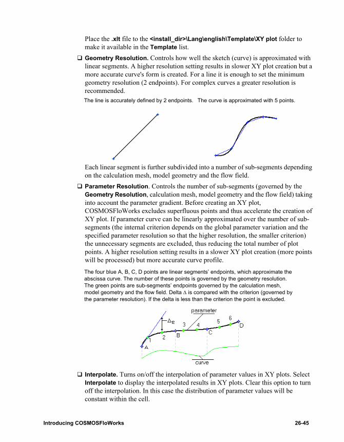
Place the .xlt file to the <install_dir>\Lang\english\Template\XY plot folder to make it available in the Template list.Geometry Resolution. Controls how well the sketch (curve) is approximated with linear segments. A higher resolution setting results in slower XY plot creation but a more accurate curve's form is created. For a line it is enough to set the minimum geometry resolution (2 endpoints). For complex curves a greater resolution is recommended.
Each linear segment is further subdivided into a number of sub-segments depending on the calculation mesh, model geometry and the flow field.Parameter Resolution. Controls the number of sub-segments (governed by the Geometry Resolution, calculation mesh, model geometry and the flow field) taking into account the parameter gradient. Before creating an XY plot, COSMOSFloWorks excludes superfluous points and thus accelerate the creation of XY plot. If parameter curve can be linearly approximated over the number of sub-segments (the internal criterion depends on the global parameter variation and the specified parameter resolution so that the higher resolution, the smaller criterion) the unnecessary segments are excluded, thus reducing the total number of plot points. A higher resolution setting results in a slower XY plot creation (more points will be processed) but more accurate curve profile.
Interpolate. Turns on/off the interpolation of parameter values in XY plots. Select Interpolate to display the interpolated results in XY plots. Clear this option to turn off the interpolation. In this case the distribution of parameter values will be constant within the cell.
The line is accurately defined by 2 endpoints. The curve is approximated with 5 points.
The four blue A, B, C, D points are linear segments’ endpoints, which approximate the abscissa curve. The number of these points is governed by the geometry resolution. The green points are sub-segments’ endpoints governed by the calculation mesh, model geometry and the flow field. Delta ∆ is compared with the criterion (governed by the parameter resolution). If the delta is less than the criterion the point is excluded.
Introducing COSMOSFloWorks 26-45
Chapter 26 Getting Results
Display boundary layer. Displays or hides boundary layers used within XY-Plots. Displaying the boundary layer will take more computer resources to visualize. Clear this option for faster creation of the XY-plot. When cleared, the parameter distribution at the boundary layer is ignored.Use CAD Geometry. By default, COSMOSFloWorks shows the original model while displaying results. Depending on how exact the model is resolved by the computational mesh, the original model’s geometry may differ slightly from the geometry on which the calculation is performed. Clear this option to see this COSMOSFloWorks-interpreted geometry instead of the model. See also "Check Geometry" on page 22-16.Click At given number of points and specify Number of points to output parameter values at the specified number of the curve's points equidistantly taken along the curve.
6 For the X, Y and Z components of the vector used to visualize a vector parameter you can select a coordinate system in which the components are calculated. By default, the Global Coordinate System is selected. You can replace the default coordinate system by selecting your coordinate system in the FeatureManager tree. To create a coordinate system click Insert, Reference Geometry, Coordinate System.
7 Click OK.
Displaying Surface Parameters
Allows you to display parameter values (minimum, maximum, average and integral) calculated over the specified surface. The values are displayed on the Local, Integral and Table tabs (the Table tab is only for time-dependent analysis). The data can also be exported into an Excel workbook.
For a time-dependent analysis you can create Excel charts and tables to display how parameters change in time. See "Scenario for Surface Parameters" on page 26-47.
All parameters are divided into two categories: Local and Integral. For local parameters (pressure, temperature, velocity etc.) the maximum, minimum and average values are evaluated.
To display surface parameters:
1 Click FloWorks, Results, Insert, Surface Parameters.– or –In the COSMOSFloWorks analysis tree, under Results, right-click the Surface Parameters folder and select Insert.TIP: If you want to create a copy of the existing surface parameters feature, right click the corresponding surface parameters icon and select Clone.
2 Select Faces for which you want to display parameter values.
26-46
3 The SurfaceParameters.xlt file is used to organize data inside an Excel document. The easiest way to create a new template is to copy the standard .xlt file and make changes to the copy to ensure that the macro which does the data exchange with COSMOSFloWorks is available. If you are experienced in macro definition, you can modify macros to display data in Excel sheets in your own way.Place the .xlt file to the <install_dir>\Lang\english\template\SurfaceParameters folder to make it available in the Template list.
4 For torque and force parameters you can specify a Coordinate system in which the x, y and z components are calculated.You can replace the default coordinate system by selecting your coordinate system in the FeatureManager tree. To create a coordinate system click Insert, Reference Geometry, Coordinate System.For forces set on non-closed surfaces, the actual force value is the displayed value plus the Reference Pressure multiplied by the surface area. The Reference Pressure value can be viewed in the Results Summary.
5 For a time-dependent (transient) analysis, additional Transient and Table tabs appear. On the Table tab, all available parameters are displayed for the Current time instant selected on the Transient tab and for time instants specified in the Scenario dialog box. On the Transient tab you access the Scenario dialog box and specify the time instant for which Local and Integral parameters are calculated.
6 Click Apply to calculate Surface Parameters.7 Click Excel if you want to calculate surface parameters and import data into Microsoft
Excel.8 Click OK to save the current definition of Surface Parameters and close the dialog
box. To change the definition of Surface Parameters, right-click the Surface Parameters feature in the COSMOSFloWorks analysis tree and select Edit Definition.
Scenario for Surface ParametersTo access the Scenario dialog box, click Scenario on the Transient tab of the Surface Parameters dialog box.
In the Scenario dialog box you specify the time instants for which Surface Parameters are calculated. For each specified time instant, surface parameters are displayed on the Table tab and in the Excel document. On the Local and Integral tabs you view only parameters calculated for a time selected by you in the Current time list on the Transient tab.
To specify a time instant to display surface parameters, select the time instant in the Available results list and click Add. The available time instants are specified in the Wizard’s Time Settings dialog box or in the Calculation Control Options dialog box during the definition of the time-dependent task.
To add all available time moments in chronological order, click Reset.
Introducing COSMOSFloWorks 26-47

Chapter 26 Getting Results
Displaying Volume Parameters
Allows you to display parameter values (minimum, maximum, average, bulk average and integral) calculated within the specified volumes (part or subassembly components in assemblies, as well as bodies in multibody parts) within the Computational Domain.
Parameters are calculated in fluid or solid depending on the component state (as fluid or solid, which can be changed in Component Control).
The values are displayed on the Local, Integral and Table tabs (the Table tab is only for time-dependent analyses). The data can also be exported into an Excel workbook.
For a time-dependent analysis you can create Excel charts and tables to display how parameters change in time. See "Scenario for Volume Parameters" on page 26-49.
All parameters are divided into two categories: Local and Integral. For local parameters (pressure, temperature, velocity etc.) the maximum, minimum, average and bulk average (mass averaged) values are evaluated. The Integral parameters are mass and volume.
To display volume parameters:
1 Click FloWorks, Results, Insert, Volume Parameters.– or –In the COSMOSFloWorks analysis tree, under Results, right-click the Volume Parameters icon and select Insert Volume Parameters.TIP: If you want to create a copy of the existing volume parameters feature, right click the corresponding volume parameters icon and select Clone.
2 In the graphics area click a face, edge or a point to select a component for which you want to specify the volume goals. You can also select a component in the FeatureManager tree.
3 The VolumeParameters.xlt file is used to organize data inside an Excel document. The easiest way to create a new template is to copy the standard .xlt file and make changes to the copy to ensure that the macro which does the data exchange with COSMOSFloWorks is available. If you are experienced in macro definition, you can modify macros to display data in Excel sheets in your own way.Place the .xlt file to the <install_dir>/Lang/english/template/VolumeParameters folder to make it available in the Template list.
4 For velocity parameters you can specify a Coordinate system in which the x, y and z components are calculated. You can replace the default coordinate system by selecting your coordinate system in the FeatureManager tree. To create a coordinate system click Insert, Reference Geometry, Coordinate System.
5 For a time-dependent (transient) analysis, additional Transient and Table tabs appear. On the Table tab, all available parameters are displayed for the Current time instant selected on the Transient tab and for time instants specified in the Scenario dialog box. On the Transient tab you access the Scenario dialog box and specify the time instant for which Local and Integral parameters are calculated.
26-48

6 Click Evaluate to calculate volume parameters.7 Click Excel if you want to calculate volume parameters and export data into Microsoft
Excel.8 Click OK to export data into Microsoft Excel, save the current definition of Volume
Parameters and close the dialog box. To change the definition of Volume Parameters, right-click the Volume Parameters feature in the COSMOSFloWorks analysis tree and select Edit Definition.
Scenario for Volume ParametersTo access the Scenario dialog box, click Scenario on the Transient tab of the Volume Parameters dialog box.
In the Scenario dialog box you specify the time instants for which Volume Parameters are calculated. For each specified time instant, Volume parameters are displayed on the Table tab and in the Excel document. On the Local and Integral tabs you view only parameters calculated for a time selected by you in the Current time list on the Transient tab.
To specify a time instant to display volume parameters, select the time instant in the Available results list and click Add. The available time instants are specified in the Wizard’s Time Settings dialog box or in the Calculation Control Options dialog box during the definition of the time-dependent task.
To add all available time moments in chronological order, click Reset.
Displaying Point Parameters
Displays parameter values at specified points inside the Computational Domain. The point of interest can be specified by its coordinates or can be selected on a plane or surface. You can also define a grid so the points will be taken at the intersections of the grid lines. The point parameters are displayed on the Table tab or can be exported into an Excel workbook.
For a time-dependent analysis you can create Excel charts and tables to display how parameters change in time. See "Scenario for Point Parameters" on page 26-52.
To display point parameters:
1 Click FloWorks, Results, Insert, Point Parameters.– or –In the COSMOSFloWorks analysis tree, under Results, right-click the Point Parameters folder and select Insert.TIP: If you want to create a copy of the existing point parameters feature, right click the corresponding point parameters icon and select Clone.
2 Select the desired Point picking mode:
Introducing COSMOSFloWorks 26-49

Chapter 26 Getting Results
• Grid. By using a grid you can specify a set of points, so the points are taken at the intersections of the grid lines. To define the grid specify either the spacing between the grid lines or the direct number of points. The points are uniformly distributed over that part of the reference plane or surface which is inside of the computational domain.
• One by One. Allows you to specify the desired points one by one. To specify a point you can type its coordinates or click in the graphics area to select it on the reference plane or planar face.
3 Specify points for which parameter values are evaluated:If One by One is selected there are two ways to specify a point:
• Type the X, Y and Z point coordinates and click Add.• Select a plane or planar face. The only requirement for assemblies is that you
must use planes that belong to the top-level assembly. Use the arrows or type a value in the Plane position box to move the plane. Orient the plane as desired. We recommend that you use the Normal To view while you select points. Click Fix to make the point selection available.
Click in the graphics area to define a point on the plane and click Add. If Auto add is selected then points are automatically inserted into the Table. The Table contains all points, regardless of the way they were specified. To remove mistakenly inserted points from the Table, see "Point Parameters Table" on page 26-51.
If Grid is selected you can define the grid in two ways:• Select a plane or surface. The only requirement for assemblies is that you must
use planes that belong to the top-level assembly. If a plane is selected, move the plane to the position you want by using the arrows or type a value in the Plane position box.In the Define grid by list select Number and specify the Number of points that will be uniformly distributed over that part of the selected plane or surface, which is inside the computational domain.
• Select a plane or surface. The only requirement for assemblies is that you must use planes that belong to the top-level assembly. If a plane is selected, move the plane to the position you want using the arrows or type a value in the Plane position box.In the Define grid by list select Spacing and specify the distance between neighboring lines of the grid. For non-planar surfaces the specified grid is projected to the surface.
You can copy coordinate values from Excel. Create a table of points in Excel. The x, y and z coordinates must be specified one after another in a row (the same as on the Table tab). Copy the table into the Clipboard, then on the Table tab press Ctrl+V. All points that are inside the computational domain will be inserted into the Table.
26-50
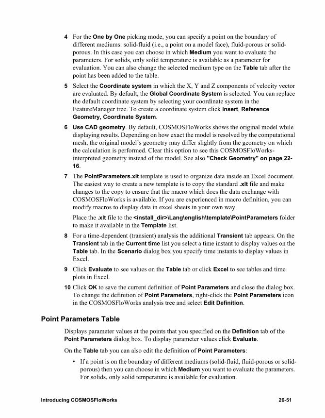
4 For the One by One picking mode, you can specify a point on the boundary of different mediums: solid-fluid (i.e., a point on a model face), fluid-porous or solid-porous. In this case you can choose in which Medium you want to evaluate the parameters. For solids, only solid temperature is available as a parameter for evaluation. You can also change the selected medium type on the Table tab after the point has been added to the table.
5 Select the Coordinate system in which the X, Y and Z components of velocity vector are evaluated. By default, the Global Coordinate System is selected. You can replace the default coordinate system by selecting your coordinate system in the FeatureManager tree. To create a coordinate system click Insert, Reference Geometry, Coordinate System.
6 Use CAD geometry. By default, COSMOSFloWorks shows the original model while displaying results. Depending on how exact the model is resolved by the computational mesh, the original model’s geometry may differ slightly from the geometry on which the calculation is performed. Clear this option to see this COSMOSFloWorks-interpreted geometry instead of the model. See also "Check Geometry" on page 22-16.
7 The PointParameters.xlt template is used to organize data inside an Excel document. The easiest way to create a new template is to copy the standard .xlt file and make changes to the copy to ensure that the macro which does the data exchange with COSMOSFloWorks is available. If you are experienced in macro definition, you can modify macros to display data in excel sheets in your own way. Place the .xlt file to the <install_dir>\Lang\english\template\PointParameters folder to make it available in the Template list.
8 For a time-dependent (transient) analysis the additional Transient tab appears. On the Transient tab in the Current time list you select a time instant to display values on the Table tab. In the Scenario dialog box you specify time instants to display values in Excel.
9 Click Evaluate to see values on the Table tab or click Excel to see tables and time plots in Excel.
10 Click OK to save the current definition of Point Parameters and close the dialog box. To change the definition of Point Parameters, right-click the Point Parameters icon in the COSMOSFloWorks analysis tree and select Edit Definition.
Point Parameters TableDisplays parameter values at the points that you specified on the Definition tab of the Point Parameters dialog box. To display parameter values click Evaluate.
On the Table tab you can also edit the definition of Point Parameters:
• If a point is on the boundary of different mediums (solid-fluid, fluid-porous or solid-porous) then you can choose in which Medium you want to evaluate the parameters. For solids, only solid temperature is available for evaluation.
Introducing COSMOSFloWorks 26-51

Chapter 26 Getting Results
• You can edit point coordinates directly in the table. To edit point coordinates, double-click the cell and enter the desired value.
• To delete a point from the table, select the point row and click Delete.
Scenario for Point ParametersTo access the Scenario dialog box, click Scenario on the Transient tab of the Point Parameters dialog box.
In the Scenario dialog box you specify time points to display Point Parameters in the Excel document. On the Table tab you view only parameters calculated for a time selected by you in the Current time list on the Transient tab.
To specify a time instant to display point parameters, select the time instant in the Available results list and click Add. The available time instants are specified in the Wizard’s Time Settings dialog box or in the Calculation Control Options dialog box during the definition of the time-dependent task. To add all available time moments in chronological order, click Reset.
Creating a Goal Plot
Allows you to study goal changes in the course of the calculation. COSMOSFloWorks uses Microsoft Excel to display goal plot data. Each goal plot is displayed in separate sheet. The Summary sheet displays goal values at the moment of finishing the calculation (or at the loaded time moment for time-dependent analyses). See "Goal Table" on page 25-6 for the meaning of the displayed values.
To create a goal plot:
1 Click FloWorks, Results, Goals.– or –In the COSMOSFloWorks analysis tree, under Results, right-click the Goals icon and select Create.
2 In the Select goals list select goals you want to display by selecting checkboxes at the left of each goal's name.If you want to make available only the goals related to the specific physical parameter, select this parameter in the Goal filter list.
3 Specify the following Plot options: Abscissa. Allows you to specify the chart abscissa parameter.
• CPU time. The chart abscissa is the overall CPU time in which the goal has been calculated (in seconds).
• Iterations. The chart abscissa is the iteration number.• Travels. The chart abscissa is the number of travels.
26-52

• Physical time. The chart abscissa is the physical time (only for time-dependent analysis).
Template. The goals.xlt file is used to organize data inside an Excel document. The easiest way to create a new template is to copy the standard .xlt file and make changes to the copy to ensure that the macro which does the data exchange with COSMOSFloWorks is available. If you are experienced in macro definition, you can modify macros to display data in excel sheets in your own way.
Place the .xlt file to the <install_dir>\Lang\english\template\Goals folder to make it available in the Template list.
4 Click OK.
Save Image
Customized Saving Images without VisualizationAllows you to save the existing Cut Plot, 3D Profile Plot, Surface Plot and Isosurfaces as an image of the specified format, size and name without visualization of a plot in the graphics area. By default images are saved in the project directory accessible by clicking FloWorks, Project, Open Project Directory., but you can also specify the desired directory where to save the image file.
To save image without visualization:
1 In the Analysis tree, right-click the cut plot, 3d profile plot, surface plot or isosurface item and select Save As.
2 Select the desired Format of the image:• BMP. Specify the Color depth. When you reduce the color depth of an image, you
limit the number of colors used with the gain of the smaller image size: 8 bit – 256 colors (the smallest file size), 16 bit – 65,536 colors (middle file size), 24 bit – the entire palette (largest file size). Select Save geometry if you want the model geometry to be shown on the saved image.
• JPG. Select the quality of the image from Best compression (lowest image quality) to Best quality (largest file size). Select Save geometry if you want the model geometry to be shown on the saved image.
• VRML. Select Save geometry if you want to save the model geometry with the image.
• eDrawings. Select Save geometry if you want to save the model geometry with the image.
3 If you selected BMP or JPG format, click Orientation to specify the orientation of the image. See also "Selecting Model Orientation" on page 26-54.
4 Click Image Dimensions and specify the image resolution in pixels.
Introducing COSMOSFloWorks 26-53

Chapter 26 Getting Results
5 In the File box, type the full path and file name of the image or click Browse and select the desired directory and type the file name.
6 If you want to access the directory where the image file will be saved, click Explore. By default, this directory is the project directory.
7 Click OK to save the image and close the dialog box, or click Apply to save the image and proceed with the dialog box.
Selecting Model OrientationAllows you to choose orientation of the model when you save a plot as an image without visualization in the graphics area.
• Select one of the standard views: Front, Back, Left, Right, Top, Bottom, or Isometric.
• For cut plots, select Normal to plane to orient the model normal to the cut plot’s section plane.
• To select an arbitrary view click Custom, orient the model in the graphics area as desired and click Pick to save the view.
Saving the Active View As an ImageAllows you to save the active view as a bitmap image of specified size and name.
To save the active view:
1 Click FloWorks, Results, Image, Save Image.2 Specify the desired Image resolution in pixels.3 Choose how the image file name is defined:
Remember last name. The file name of the image is taken from the last saving. This is useful if you want to replace the previously created file. To avoid replacing, you can edit the File name or browse for an alternate folder where the file will be saved. But if you want to create a set of files, it is better to use a template-based name.Use template. The file name is based on the specified template. This is useful when you want to create a set of files with descriptive names. The following parameters can be specified in the template:
• Plot Name. The name of the first displayed plot (cut plot, surface plot or isosurface) in the COSMOSFloWorks analysis tree.
• Plot Parameters. Physical parameters of the first displayed plot and parameter of the displayed isosurface.
• Iteration\Time. The iteration number or time moment (for time-dependent analyses) when the calculation was stopped.
• Number. The unique number.
26-54

The resulting file name is shown in the File box. You can also edit a template by typing the desired description in the Template box.
4 Click OK.
Creating a Report
COSMOSFloWorks allows you to create an analysis report using Microsoft Word.
You can add information either to an existing Word document or create a new document based on the COSMOSFloWorks pre-defined or custom template.
To create a report based on a template:
1 Click FloWorks, Results, Report.– or –In the COSMOSFloWorks analysis tree, under Results, right-click the Report icon and select Create.
2 Click From Template. In the Open dialog box you can select one of the COSMOSFloWorks pre-defined report templates (id*.dot) or browse for a custom template containing the ID that are replaced with the information from the active COSMOSFloWorks project. The following standard templates are available:
• id_fullreport.dot – generates a text report including all available information about the current project in a brief form (all “short” IDs are used).
• idf_fullreport.dot - generates a text report including all available information about the current project in a full form (all “full” IDs are used; the fullest report).
• id_inputdata.dot – generates a text report of the project’s input data in a brief form.
• idf_inputdata.dot - generates a text report of the project’s input data information in a full form.
• id_results.dot - generates a text report of only the results information in a brief form.
See "Report IDs" on page 26-57 for more details about the available IDs and their brief and full forms.
3 Select the desired template and click Open. The newly created document appears in the Available target documents list.
4 If you want to add pictures, Excel sheets or ID-based project information, to the report, select the document in the Available target documents list and click Attach. Information from the Pictures and Charts and IDs tabs will be added to each document with the Attached status set to Yes after clicking Add to Report on the corresponding tab. See details below on how to add the project information to an existing document.
5 Go to Word and save the document.
Introducing COSMOSFloWorks 26-55

Chapter 26 Getting Results
To create a custom template:
1 Click FloWorks, Results, Report.– or –In the COSMOSFloWorks analysis tree, under Results, right-click the Report item and select Create.
2 Click New Template.3 Go to the IDs tab and select Insert IDs only.4 Specify IDs you want to add to the template:
a) In the IDs for insertion list, select an ID you want to add into the custom template. See "Report IDs" on page 26-57 for details. IDs have a parent-child structure: a parent ID contains all information of its child IDs.
b) Select either the Full or Short ID’s form. For simple data the “Full” form differs from the “Short” form only by the caption (e.g., Full form: Operating System: Windows NT v4.0 Service Pack 6; Short form: Windows NT v4.0 Service Pack 6). For complex data, such as coordinate or time-dependent conditions, the “Full” form will contain the specified dependency.
c) Specify the location inside the document where the selected ID should be added. Choose either to add the ID at the current cursor position or at the end of the document. To define a cursor position within a Word document it is convenient to use the On Top button. When the On Top button is pressed, the Report dialog box is displayed on top of the other windows.
d) Click Add to Report.
5 Go to Word and save the document.
To add information to an existing document:
1 Click FloWorks, Results, Report.– or –In the COSMOSFloWorks analysis tree, under Results, right-click the Report item and select Create.
2 Choose to add the information either into an existing file or a new file:• Click Open File. In the Open dialog box browse for the existing .doc file, then
click Open. The file name appears in the Available target documents list. The Available target documents list displays all currently opened documents. You can simultaneously add information to more than one document. In the Available target documents list select a document to which you want to add the current project information and click Attach.
• Click New Document.3 On the Picture and Charts tab specify images and/or Excel sheets that you want to add
to the report:
26-56

a) Specify the location within the document where you would like to add the selected pictures or charts. Choose either to add the information at the current cursor position or at the end of the document. To define a cursor position within a Word document it is convenient to use the On Top button. When the On Top button is pressed, the Report dialog box is displayed on top of the other windows.
b) Choose to add either Current image (active view) or Image from file (.bmp), or Excel sheet from file (*.xls). Be aware that you can add only the current sheet of the specified Excel workbook. If the workbook is currently closed, the default sheet will be taken (a sheet that appears after opening the workbook).
c) Click Add to Report (and browse to the image or Excel file you want to add).
4 On the IDs tab specify which project information to add to the report. To add the information you need, select the associated ID:
a) In the list of IDs for insertion, select an ID associated with the project data you want to output into the report. See "Report IDs" on page 26-57 for details. IDs have a parent-child structure: a parent ID contains all information of its child IDs.
b) Select the way (Full or Short) in which information is displayed. For simple data the “Full” form differs from the “Short” form only by the caption (e.g., Full form: Operating System: Windows NT v4.0 Service Pack 6; Short form: Windows NT v4.0 Service Pack 6). For complex data, such as coordinate or time-dependent conditions, the “Full” form will contain the specified dependency.
c) Specify the location inside the document where the project data associated with the selected ID should be added. Choose either to add the information at the current cursor position or at the end of the document. To define a cursor position within a Word document it is convenient to use the On Top button. When the On Top button is pressed, the Report dialog box is displayed on top of the other windows.
d) Click Add to Report.5 Go to Word and save the document.
Report IDsThe template defines how the information is arranged inside the document. The data exchange is done directly by COSMOSFloWorks. The report generator searches the template for special IDs and replaces the IDs with the information from the active COSMOSFloWorks project. In addition to the standard templates (id*.dot), you can specify your own template by creating a Microsoft Word template (*.dot) and insert any ID that will be replaced with the corresponding project information.
Introducing COSMOSFloWorks 26-57

Chapter 26 Getting Results
The list of IDs has a parent-child structure: a parent ID contains all information of its child IDs. Some IDs have two forms - the “full” form (with the “IDF_” prefix) and the “short” form (with the “ID_” prefix). For simple data the “full” form differs from the “short” one only by the caption (e.g., full form: Operating System: Windows NT v4.0 Service Pack 6; short form: Windows NT v4.0 Service Pack 6). For complex data, such as coordinate or time-dependent conditions, the “full” form will contain the specified dependency.
To see the ID description, select the ID in the IDs for insertion list.
Default Reference Parameters
Allows you to manually specify values of the default reference fluid temperature, reference pressure, reference velocity and reference density. These values are used by COSMOSFloWorks for calculating the following parameters:
• The heat transfer coefficient
,
where q is the heat flux from the wall to the fluid, calculated by COSMOSFloWorks, TS is the wall temperature calculated by COSMOSFloWorks, Tf is the Default reference fluid temperature. The default reference fluid temperature is applied by default to all walls in the model.
• The friction coefficient on the wall surface
where τw is the fluid’s shear stress at the wall surface, calculated by COSMOSFloWorks, ρref is the Reference density, Vref is the Reference velocity in the absolute (i.e. non-rotating) coordinate system.
• The Stanton number
,
where h is the heat transfer coefficient at the wall, calculated by COSMOSFloWorks, CP is the fluid’s specific heat at constant pressure, ρref is the Reference density, Vref is the Reference velocity in the absolute (i.e. non-rotating) coordinate system.
fS TTqh−
=
25,0 refref
wf V
Cρτ
=
refrefP VChSt
ρ=
26-58

• In some cases when determining the force acting on a surface you need to take into account the reference pressure. The total force acting on the surface is the sum of the friction and pressure forces and is defined as:
,
where is the friction force calculated by COSMOSFloWorks, is the pressure force calculated by COSMOSFloWorks, τw is the fluid’s shear stress at the wall surface’s element of dS area, calculated by COSMOSFloWorks, P is the calculated static pressure acting on the wall surface’s element of dS area and Pref is the Reference pressure acting on the wall surface’s element of dS area.
To specify default reference parameters:
1 Click FloWorks, Results, Default Reference Parameters.2 Specify the value of the Default reference fluid temperature and/or adjust values of
the other two reference parameters.• Select Adjust reference pressure to specify the Reference pressure value.• Select Adjust reference velocity and density to specify the Reference velocity
and Reference density values.3 Click OK.
Specifying Reference Fluid TemperatureAllows you to manually specify an appropriate reference fluid temperature for visualizing the heat transfer coefficient h (see above).
To set the reference fluid temperature for a wall:
1 Click FloWorks, Results, Insert, Reference Parameters.2 In the graphics area select the model faces, on which you intend to display the heat
transfer coefficient distribution. These faces appear in the Faces to apply the reference fluid temperature list. To remove a face from this list, select it in the list and press the Delete key, or you can select the face again in the graphics area.
3 Specify the Reference fluid temperature value.4 Click OK.
Animation of Results
There are two types of animations to help you understand flow behavior in space and in time.
For both steady and time-dependent (transient) problems you can animate flow trajectories, cut plots, 3D profile plots and isosurfaces to visualize the flow behavior in
∫∫∫ −+=+=S
refSS
wpf SdPSPdSdFFFrrrrrr
τ
fFr
pFr
Introducing COSMOSFloWorks 26-59

Chapter 26 Getting Results
space (in case of a time-dependent problem the animated results are related to the currently loaded time instant).
For time-dependent problems it is also possible to animate Cut Plots, Surface Plots, 3D Profile Plots, Flow Trajectories, Particles Trajectories and Isosurfaces to visualize how a parameter distribution changes in time.
To animate results of a time-dependent problem:
1 Load results for any time instant.2 Create result features (cut plots, 3D profile plots, surface plots, flow trajectories,
particle trajectories or isosurfaces) you want to animate. 3 Click FloWorks, Results, Transient Animation. The Animation dialog box appears.4 Click Scenario and specify time instants to animate results.5 Specify the name of the .avi file and Frame rate. Additionally you can save a series of
bitmap images to create movies in another format.6 Click Create. COSMOSFloWorks creates a Windows-based .avi file. Click Play to run
the animation using the default Windows player.
Creating an AnimationAllows you to set animation options, generate an animation and play it using the standard Windows player.
To create an animation:
1 Specify the way animation is created:• Static frames. Select the BMP files check box if you want to save each frame as
a bitmap image for creating movies in your own format. Specify the Location folder for bitmap series and type the file name prefix in the Name template box. The file name is generated from this prefix and the number of the frame.
• Movie. Select the AVI file check box and browse to the folder where you want to save the .avi file and specify the Frame rate (i.e. number of frames per second) for the animation. Select the Compressed (Microsoft Video 1) check box if you want the animation to be compressed with the Microsoft Video 1 (MS-CRAM) video compression codec. This compression method does not impact the animation quality.
2 If you animate a time-dependent analysis, click Scenario to specify time instants, for which you want to animate results.
3 Click Create. After generating the animation, COSMOSFloWorks saves it as a Windows-based .avi file. Click Play to run the animation using the default Windows player.
26-60

Scenario for Time - Dependent AnalysisIn the Scenario dialog box you specify time instants to animate results of a time-dependent (transient) analysis. Each frame displays a flow parameter distribution at the specified time instant.
To specify time instants for animation of time-dependent analysis:
1 FloWorks, Results, Transient Animation.2 In the Animation dialog box click Scenario.3 In the Available results list select a time instant and click Add. The available time
instants are specified in the Wizard’s Time Settings dialog box or in the Calculation Control Options dialog box during the definition of the time-dependent task.To add all available time moments in chronological order, click Reset.
4 Click OK.
List of Parameters and Their Definitions
• Pressure is the static pressure for gases and liquids.• Total pressure
For liquids: Total pressure = Pressure + Dynamic pressure (in the non-rotating coordinate system), it is valid in the absolute (i.e., non-rotating) coordinate system only;
For gases: Total pressure , where P is the flow’s
static pressure, ã is the gas’s specific heat ratio, M is the flow’s Mach number.
• Dynamic pressureDynamic head q = ρV2/2, where ρ is the fluid density, V is the fluid velocity (i.e., the velocity vector’s absolute value), it is valid in the absolute (i.e., non-rotating) coordinate system only.
• Density is the mass per unit volume of the fluid.• Velocity is the fluid velocity vector's absolute value in the absolute (i.e., non-
rotating) coordinate system.• Velocity RRF is the fluid velocity vector's absolute value in the rotating coordinate
system.• Temperature is the static temperature value of the fluid and/or solid body.• X (Y, Z)-velocity is the fluid velocity vector's component along the Cartesian
coordinate system's X (Y, Z) coordinate axis.• X (Y, Z)-velocity RRF is the fluid velocity vector's component along the rotating
Cartesian coordinate system's X (Y, Z) coordinate axis.
1γγ
2
21-γ1
−
+⋅= MPP0
Introducing COSMOSFloWorks 26-61

Chapter 26 Getting Results
• Mach number M = V/a, where V is the fluid velocity (i.e., the velocity vector’s absolute value) in the selected (i.e., absolute or rotating) coordinate system, a is the local (i.e., at the point under consideration) fluid flow sonic velocity.
• Turbulent viscosity , where k is the turbulent kinetic
energy, ε is the turbulent dissipation, is a turbulent viscosity factor. Turbulent viscosity is the addition to the laminar (i.e., molecular) fluid viscosity in order to obtain the turbulent flow shear stress.
• Turbulent time , where k is the turbulent kinetic energy, ε is the turbulent dissipation, both are calculated by solving the corresponding differential equations in the used k-ε model of turbulence.
• Turbulent length , where Cµ = 0.09, k is the turbulent kinetic
energy, ε is the turbulent dissipation, both are calculated by solving the corresponding differential equations in the used k-ε model of turbulence; it is a length characteristic of larger turbulent eddies.
• Turbulence intensity , where k is the turbulent kinetic energy,
V is the time-average fluid velocity.• Turbulent energy k is the turbulent kinetic energy defined as .
• Turbulent dissipation ε is the turbulent kinetic energy dissipation• Friction coefficient is the coefficient Cf of fluid friction on the wall surface:
, where is the fluid shear stress at the wall surface, ρ is the
fluid density, U0 is the fluid velocity at the boundary layer’s outer boundary, it is valid in the absolute (i.e., non-rotating) coordinate system only.
• Stanton number St = h/(ρ ·cp·U0), where h is the heat transfer coefficient at the wall, ρ is the fluid density, cp is the fluid’s specific heat at constant pressure, U0 is the fluid velocity at the boundary layer’s outer boundary, it is valid in the absolute (i.e., non-rotating) coordinate system only
• Heat transfer coefficient h = q/(Tw-Tf), where q is the calculated heat flux from the wall to the fluid, Tw is the calculated wall temperature, Tf is the reference fluid temperature specified by user.
• Shear stress is the fluid shear stress at the wall surface, it is valid in the absolute (i.e., non-rotating) coordinate system only.
ερ
µ µµ
2kCft
⋅⋅⋅=
µfµµ =l
ετ /k=
εµ
23750 /.
t
kCL =
232
%100V
kIt ⋅=
'i
i
'iuuk ∑
=
=3
121
2050 U.
C wf ⋅⋅
=ρ
τwτ
wτ
26-62

• Surface heat flux is the heat flux from the wall to the fluid (positive values) or from the fluid to the wall (negative values).
• Heat flux is the absolute value of the heat flux in solid body vector.• Specific heat CP is the fluid’s specific heat at constant pressure.• Dynamic viscosity µ is the fluid’s dynamic viscosity.• Prandtl number Pr = CP ·µ/k, where CP is the fluid’s specific heat at constant
pressure, µ is the fluid’s dynamic viscosity, k is the fluid’s thermal conductivity.• Mass fraction is the mass of a fluid component (species) per unit mass of the
mixture.• Volume fraction is the volume of a fluid component (species) per unit volume of
the mixture• Net radiant flux is the difference between the radiant heat leaving the surface and
the radiant heat flux entering the surface.• Leaving radiant flux is the flux of the heat radiated from the surface, i.e. the radiant
heat flux leaving the surface.• Fluid temperature is the static temperature for gases and liquids.• Solid temperature is the temperature of solid bodies.• Stagnation temperature (for gases only) defined as total temperature =
temperature + V2/(2·CP), where V is the gas velocity in the absolute (i.e., non-rotating) coordinate system, CP is the gas specific heat at constant pressure, it is valid in the absolute (i.e., non-rotating) coordinate system only.
• Stagnation density (for gases only) ρ0 is the gas total density corresponding to the gas total pressure (P0) or the gas total temperature (T0), e.g. for isentropic flows: ρ0 = ρ·(P0/P)1/k or ρ0 = ρ·(T0/T)1/(k - 1), where k is the gas isentropic exponent, it is valid in the absolute (i.e., non-rotating) coordinate system only.
• Cartesian X, Y, Z are the point’s coordinates in the Cartesian coordinate system in which the calculation is performed.
• Phi (cylindrical) is the point’s φ coordinate in the cylindrical coordinate system selected in the postprocessor by selecting this system’s axis.
• Radius r (cylindrical) is the point’s radial coordinate in the cylindrical coordinate system selected in the postprocessor by selecting this system’s axis.
• Z-axis (cylindrical) is the point’s axial coordinate in the cylindrical coordinate system selected in the postprocessor by selecting this system’s axis.
• Phi (spherical) is the point’s φ coordinate in the spherical coordinate system based on the origin of the Cartesian Coordinate system selected in the postprocessor.
• Theta (spherical) is the point’s θ coordinate in the spherical coordinate system based on the origin of the Cartesian Coordinate system selected in the postprocessor.
Introducing COSMOSFloWorks 26-63

Chapter 26 Getting Results
• Position vector R (spherical) is the point’s radial coordinate in the spherical coordinate system based on the origin of the Cartesian Coordinate system selected in the postprocessor.
• Axial velocity is the fluid velocity component in the axial direction along the rotating coordinate system’s rotational axis, it can be determined both in the rotating coordinate system and in the absolute (i.e., non-rotating) coordinate system.
• Radial velocity is the fluid velocity component in the radial direction in the cylindrical coordinate system corresponding to the rotating coordinate system, it can be determined both in the rotating coordinate system and in the absolute (i.e., non-rotating) coordinate system.
• Circumferential velocity is the fluid velocity component along the rotating coordinate system's peripheral velocity vector in the absolute (i.e., non-rotating) coordinate system.
• Circumferential velocity RRF is a circumferential velocity in the rotating frame of reference.
• Peripheral velocity is the circumferential speed of the rotating coordinate system’s rotation: ω·r, where ω is the angular velocity at which the rotating coordinate system rotates, r is the radius of the point under consideration in the cylindrical coordinate system corresponding to the rotating coordinate system.
• Relative velocity , where V is the fluid velocity vector’s absolute value in the selected (i.e., absolute or rotating) coordinate system, a* is the critical fluid flow sonic velocity (i.e., at the point where the flow’s Mach number is equal to 1).
• Normal velocity is the fluid velocity component in the Cut Plot plane, which is normal to the Cut Plot plane.
• Tangential velocity is the fluid velocity component in the Cut Plot plane, which is tangential to the Cut Plot plane.
• Vorticity , where is
the flow velocity vector in an absolute (i.e., non-rotating) coordinate system,
and , where is the flow velocity vector in a coordinate
system rotating at the angular velocity. The vorticity is a local property of flow, it measures the solid body-like rotation of a material point P' about the neighboring
material point P, so this rotation’s velocity is equal to , where
is the vorticity at P and is the distance from P to P', it is valid in the absolute (i.e., non-rotating) coordinate system only.
*a/V*M =
yV
xV
,x
Vz
V,z
Vy
VVrot xyzxyz
∂∂
−∂
∂
∂∂
−∂
∂∂
∂−
∂∂
==ξ V
ωξ 2+= Vrot V
ω
rdVrot. ×⋅50
Vrot rd
26-64

27 COSMOSFloWorks Analysis Tree
Overview of COSMOSFloWorks Analysis Tree
As soon as a project has been created, a new COSMOSFloWorks tab appears on the right side of the panel where the FeatureManager tree, the PropertyManager and the ConfigurationManager are displayed.
The COSMOSFloWorks analysis tree provides convenience and flexibility in specifying project data and viewing results. You can also use the COSMOSFloWorks analysis tree to modify, suppress (only for Input Data items) and delete the COSMOSFloWorks features. The COSMOSFloWorks analysis tree is fully customizable; you can select which folders are shown every time you work with COSMOSFloWorks and which folders are hidden. A hidden folder become visible when you add a new feature of corresponding type. The folder remains visible until the last feature of this type is deleted.
To modify the specified data, right-click the corresponding item and select Edit Definition.
To delete an item, right-click it and select Delete. See "Confirm Delete" on page 27-3 for details.
The COSMOSFloWorks analysis tree under the Input Data folder allows you to easily specify project data that cannot be defined trough the Wizard or in the General Settings dialog box. These data are the computational domain settings (performed in the Computational Domain dialog box), boundary conditions (specified in the Boundary Conditions dialog box) and Goals. Depending on the project settings (specified in the Wizard and in the General Settings dialog box), through the COSMOSFloWorks analysis tree you can also specify Fluid Subdomains (if fluids of different types were selected), Rotating Regions (if Local region(s) of rotation option is enabled), Solid Materials (if Heat conduction in solids is enabled) and/or Radiative Surfaces (if Radiation is enabled). Other settings and features can be specified using COSMOSFloWorks menu and Toolbars. Once the feature is created and the corresponding folder appears in the COSMOSFloWorks analysis tree you can
Introducing COSMOSFloWorks 27-1

Chapter 27 COSMOSFloWorks Analysis Tree
add new features of this type using the menu available by right-clicking on the folder name.
To suppress an input data item, right-click it and select Suppress.
To access the calculation results. When the calculation has finished, all the project results are accessible from the COSMOSFloWorks analysis tree under the Results folder. All folders under the Results folder are visible by default. See "Getting Results" on page 26-1 for more detailed information.
To quickly create a copy of the existing feature from the Results folder, right-click the feature and select Clone.
To create a copy of the existing feature in another currently opened COSMOSFloWorks project, right-click the feature and select Copy to Project. See "Copy Features among Projects" on page 5-6.
Right-click the project name at the top of the COSMOSFloWorks analysis tree to perform the following:• Enable or disable Automatic Rebuild of the project.• Rebuild the project.• Show or Hide Global Coordinate system.• Clone Project.• Create Template.• Clear Configuration.• Open Project Directory. The default directory for storing project files, output
images, reports and Excel documents.• Show or Hide Basic Mesh.• Select the Basic Mesh Color.• Run the calculation for the current project. • Customize Tree. This option allows you to select features to be shown under the
Input Data and Results folders by default. Please note that this is a global COSMOSFloWorks setting and therefore affects not only the current project, but other COSMOSFloWorks projects as well.
Global Coordinate System
The Global Coordinate System is applied to all settings specified in Wizard or General Settings.
Right-click the project name at the top of the COSMOSFloWorks analysis tree and select Show Global Coordinate System or Hide Global Coordinate System to display or hide the Global Coordinate System in the graphics area.
27-2
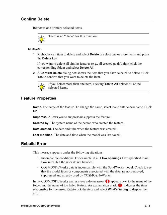
Confirm Delete
Removes one or more selected items.
To delete:
1 Right-click an item to delete and select Delete or select one or more items and press the Delete key.If you want to delete all similar features (e.g., all created goals), right-click the corresponding folder and select Delete All.
2 A Confirm Delete dialog box shows the item that you have selected to delete. Click Yes to confirm that you want to delete the item.
Feature Properties
Name. The name of the feature. To change the name, select it and enter a new name. Click OK.
Suppress. Allows you to suppress/unsuppress the feature.
Created by. The system name of the person who created the feature.
Date created. The date and time when the feature was created.
Last modified. The date and time when the model was last saved.
Rebuild Error
This message appears under the following situations:
• Incompatible conditions. For example, if all Flow openings have specified mass flow rates, but the rates do not balance.
• COSMOSFloWorks data is incompatible with the SolidWorks model. Check to see that the model faces or components associated with the data are not removed, suppressed and already used by COSMOSFloWorks.
In the COSMOSFloWorks analysis tree a down arrow appears next to the name of the folder and the name of the failed feature. An exclamation mark indicates the item responsible for the error. Right-click the item and select What’s Wrong to display the error.
There is no “Undo” for this function.
If you select more than one item, clicking Yes to All deletes all of the selected items.
Introducing COSMOSFloWorks 27-3

Chapter 27 COSMOSFloWorks Analysis Tree
After you have fixed the problem, click FloWorks, Project, Rebuild.
27-4
28 Support Service
User Information
To access COSMOSFloWorks Support Service click FloWorks, Tools, Support Service.
On the General tab, please provide the following mandatory information:First NameLast NameOccupationCompanyAddressCityCountryE-mail
The information is saved and will be restored the next time the Support Service wizard is started.
Problem Description
• In the Problem Type list select one of the predefined types. A new type may also be entered if none of the predefined types fit your criteria.
• In the Reproducible list select Yes or No.• In the Product Part list select which part of the program may be the cause of the
problem (in your opinion). If none fits, a new one may also be entered.• In the text box enter all steps, which generate the problem.
Introducing COSMOSFloWorks 28-1
Chapter 28 Support Service
Project Selection
You can add data from multiple projects to a support archive. Click the check box on the left of the configuration name to select the project where the problem was encountered.
Attachments
For the best support service on the problem, you should include some files with your request.
It is strongly recommended to add the SolidWorks Model file(s), COSMOSFloWorks Project file and COSMOSFloWorks Journal file. These files are automatically located.
Under Results, any COSMOSFloWorks result file may be added as needed to show the problem. Note that results files (.fld) may be large in size.
It is also possible to include any type of file to the support request archive under Other files. Click Attach, select the file you want to add and click Open.
All files will be stored in a single file with the .fwarc extension and will be heavily compressed to save time and cost of data transfer.
28-2

