introducing nonlinear pricing into consumer choice theoryeconomics.usf.edu/pdf/jee 33(2)...

Introducing Nonlinear Pricing into Consumer Choice TheoryAuthor(s): Joseph S. DeSalvo and Mobinul HuqSource: The Journal of Economic Education, Vol. 33, No. 2 (Spring, 2002), pp. 166-179Published by: Heldref PublicationsStable URL: http://www.jstor.org/stable/1183393Accessed: 04/10/2010 10:59

Your use of the JSTOR archive indicates your acceptance of JSTOR's Terms and Conditions of Use, available athttp://links.jstor.org/page/info/about/policies/terms.jsp. JSTOR's Terms and Conditions of Use provides, in part, that unless youhave obtained prior permission, you may not download an entire issue of a journal or multiple copies of articles, and you mayuse content in the JSTOR archive only for your personal, non-commercial use.

Please contact the publisher regarding any further use of this work. Publisher contact information may be obtained athttp://links.jstor.org/action/showPublisher?publisherCode=held.

Each copy of any part of a JSTOR transmission must contain the same copyright notice that appears on the screen or printedpage of such transmission.

JSTOR is a not-for-profit service that helps scholars, researchers, and students discover, use, and build upon a wide range ofcontent in a trusted digital archive. We use information technology and tools to increase productivity and facilitate new formsof scholarship. For more information about JSTOR, please contact [email protected].

Heldref Publications is collaborating with JSTOR to digitize, preserve and extend access to The Journal ofEconomic Education.

http://links.jstor.org

http://links.jstor.org/action/showPublisher?publisherCode=held

http://www.jstor.org/stable/1183393?origin=JSTOR-pdf

http://links.jstor.org/page/info/about/policies/terms.jsp

http://links.jstor.org/action/showPublisher?publisherCode=held

Introducing Nonlinear Pricing into Consumer Choice Theory

Joseph S. DeSalvo and Mobinul Huq

Abstract: Introducing nonlinear pricing into the teaching of consumer choice theory would provide an extension that introduces the student to a ubiquitous phenomenon and would enable the instructor to develop some interesting behavioral results. After distinguishing linear and nonlinear pricing, the authors derive the tariff, the consumer budget equation, and some behavioral implications for various nonlinear pricing policies. They show, among other things, that under some forms of nonlinear pricing, after a price rise people may buy more of a commodity or more of a commodity than would have been bought under linear pricing. They note some complications arising in the treatment of quantity discounts and premia. Key words: block-declining tariff, consumer choice theory, multi-part tariff, nonlinear pricing, quantity discounts JEL codes: A22, D11

Although second-degree price discrimination has been treated in intermediate microeconomic textbooks for years, other types of nonlinear pricing, in particular, the two-part tariff and bundling, are now frequently included as well (e.g., Browning and Zupan 1999, 314-18; Nicholson 2000, 305-07, 310-11; Pindyck and Rubinfeld 1998, 392-409; Varian 1999, 444-48). These treatments are, however, confined to the theory of the firm.

We believe that the introduction of nonlinear pricing into the teaching of consumer choice theory would benefit students for at least two reasons. First, nonlinear pricing would serve as an extension that introduces the student to a ubiquitous phenomenon. Block-declining (or tapered) tariffs, two- and three-part tariffs, and quantity discounts are pricing policies used for a variety of consumer goods, including groceries; residential electricity, telephone, and cable television service; amusement parks; and many others. Second, it would enable the instructor to develop some interesting behavioral results. For example, we show that under some forms of nonlinear pricing, people may buy more of a commodity after a price increase or more of a commodity than would have been purchased under linear pricing (e.g., a consumer may purchase 12 items because of a quantity discount on a case lot, rather than 11 individual items). Although we do not pursue it here, one can demonstrate how consumers might choose among available alternative linear or nonlinear pricing plans (e.g., for telephone and cable

Joseph S. DeSalvo is a professor of economics at the University of South Florida (e-mail: jdesalvo @coba.usfedu), and Mobinul Huq is an associate professor of economics at the University of Saskatchewan. The authors thank three anonymous reviewers for suggestions on this article.

166 JOURNAL OF ECONOMIC EDUCATION

TV). In addition, some of the comparative static results obtained under linear pricing may not be the same under nonlinear pricing.

In this article, we distinguish nonlinear and linear pricing and then discuss fairly thoroughly various types of nonlinear pricing, in each case specifying the form of the tariff and of the consumer's budget constraint as well as deducing behavioral implications. We also show that linear and nonlinear pricing are, except for quantity discounts and premia, special cases of the three-part tariff, a result that may simplify classroom presentation. We give quantity discounts and premia separate treatment.

CONTRASTING LINEAR AND NONLINEAR PRICING

In the standard theory of consumer choice, a commodity price is exogenous and invariant to quantity purchased. Consequently, the consumer's total expenditure on the good is proportional to the quantity purchased. This expenditure relationship is a tariff although it is not described that way in microeconomic theory textbooks.' For a single good, say X, the tariff may be represented algebraically:

E = PX, (1)

where E is total expenditure on X, and P is the price per unit of X. Considering only two goods, if the prices of both are exogenous and invariant to quantity purchased, then the consumer's budget line is straight and negatively sloped. For this case, assuming Y is the second good and normalizing the price of Y to unity, we have the familiar budget equation, where I denotes income,

Y = I- PX. (2) If the tariff is proportional to the quantity of the good purchased, we have lin-

ear pricing. The average price, E/X, and the marginal price, dE/dX, are equal to P, and the budget line is linear. If the tariff is not strictly proportional to the quantity purchased, we have nonlinear pricing. The average and marginal prices diverge, and the budget line may not be linear. We refer to any pricing policy in which average price varies with quantity purchased as nonlinear pricing.

The general case of nonlinear pricing may be represented by the following equation of the tariff:

E = E(X), (3) where the first E is a variable, and the second is a functional operator. Here, the average price, E/X, and the marginal price, which we denote E', are not necessarily equal. Typically E' > 0 and E" < 0, that is, the tariff increases at a decreasing rate, and there may be a fee, F, independent of X. Situations may arise in which E" > 0, for example, quantity premia or lifeline rates, to be discussed later.

Under these conditions, the equation of the budget line is

Y = I - E(X). (4)

The budget line would be strictly convex if E" < 0 and strictly concave if E" > 0 for all feasible values of X. When the budget line is convex, the standard tangency

Spring 2002 167

condition for utility maximization is not necessarily valid, and comparative static results derived in the standard case may not be valid (Moffitt 1990).

Although we have introduced the concept of nonlinear pricing with continuous and continuously differentiable functions, nonlinear pricing does not necessarily satisfy both of these conditions. In the next section, we treat specific cases of nonlinear pricing in which the tariff and the resulting budget line are piecewise linear or, in one case, linear. We return briefly to the continuous and continuously differentiable case later.

TYPES OF NONLINEAR PRICING

In this section, we describe various types of nonlinear pricing, deriving the associated tariff and budget line and investigating some behavioral properties. We treat the following cases: block-declining or tapered tariffs, two-part tariffs, three-part tariffs, and quantity discounts or premia.

Block-Declining Tariff

The block-declining tariff, also called the tapered tariff, occurs when the consumer can purchase up to X* units of a good at one price and the X*th and remaining units at a lower price. (In the pricing policies considered here, we assume at most two marginal prices although in practice there may be many.) This case is equivalent to second-degree price discrimination. It may also be con- strued as a special case of bundling.2 The tariff will take the form

( PX 0OX<X* E(X) = (p)* XX* (5)

(Pi - 2 )X * +P2X. X

> X *

If P, > P2, then this tariff appears as in Figure 1(a). Here average price is constant and equal to Pi over the first segment of the tariff, whereas it is variable and equal to P2 + [(P1 - P2)X*]/X over the second segment. The marginal price over the first segment is Pi and P2 over the second segment.

The equation of the budget line (Figure ib) is

I - PX 0X<X *

(6) I -(PI - P2 )X * -P2X. X 2 X *

With this budget line, those with weaker preferences for X (indifference curves such as ICA) will come into equilibrium on the first segment buying smaller quantities of X. Those with stronger preferences for X (indifference curves such as IC, in Figure 1B) will end up on the second segment buying larger quantities of X, thereby taking advantage of the lower marginal price. This, of course, is the essence of price discrimination.

Before turning to a couple of behavioral implications of this pricing policy, we note some existence-of-equilibrium problems associated with a kinked budget line. For purposes of this discussion, ignore the indifference curves shown in Fig- ure l(b). With differentiable indifference curves, no one will come into equilib-


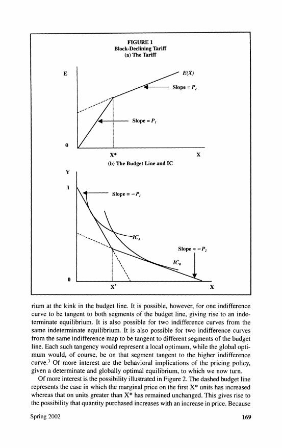
FIGURE 1 Block-Declining Tariff

(a) The Tariff

E E(X)

*. - Slope =P2

Slope=P,

X* X (b) The Budget Line and IC

I Slope = -P,

"ICA

"Slope = -P2

\ICB

0

X X

rium at the kink in the budget line. It is possible, however, for one indifference curve to be tangent to both segments of the budget line, giving rise to an indeterminate equilibrium. It is also possible for two indifference curves from the same indeterminate equilibrium. It is also possible for two indifference curves from the same indifference map to be tangent to different segments of the budget line. Each such tangency would represent a local optimum, while the global optimum would, of course, be on that segment tangent to the higher indifference curve.3 Of more interest are the behavioral implications of the pricing policy, given a determinate and globally optimal equilibrium, to which we now turn.

Of more interest is the possibility illustrated in Figure 2. The dashed budget line represents the case in which the marginal price on the first X* units has increased whereas that on units greater than X* has remained unchanged. This gives rise to the possibility that quantity purchased increases with an increase in price. Because

Spring 2002 169

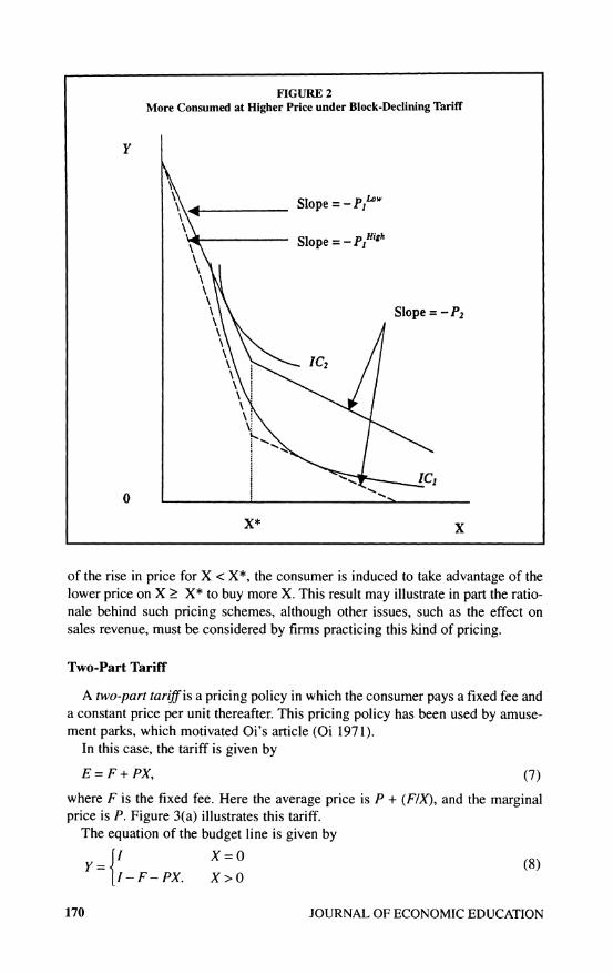
FIGURE 2 More Consumed at Higher Price under Block-Declining Tariff

Y

Slope = - PiLw

Slope = - p High

\ Slope = - Pz

X* X

of the rise in price for X < X*, the consumer is induced to take advantage of the lower price on X > X* to buy more X. This result may illustrate in part the ratio- nale behind such pricing schemes, although other issues, such as the effect on sales revenue, must be considered by firms practicing this kind of pricing.

Two-Part Tariff

A two-part tariffis a pricing policy in which the consumer pays a fixed fee and a constant price per unit thereafter. This pricing policy has been used by amusement parks, which motivated Oi's article (Oi 1971).

In this case, the tariff is given by

E = F + PX, (7) where F is the fixed fee. Here the average price is P + (FIX), and the marginal price is P. Figure 3(a) illustrates this tariff.

The equation of the budget line is given by

I-F-PX. X=0 (8) I- F- PX. X>


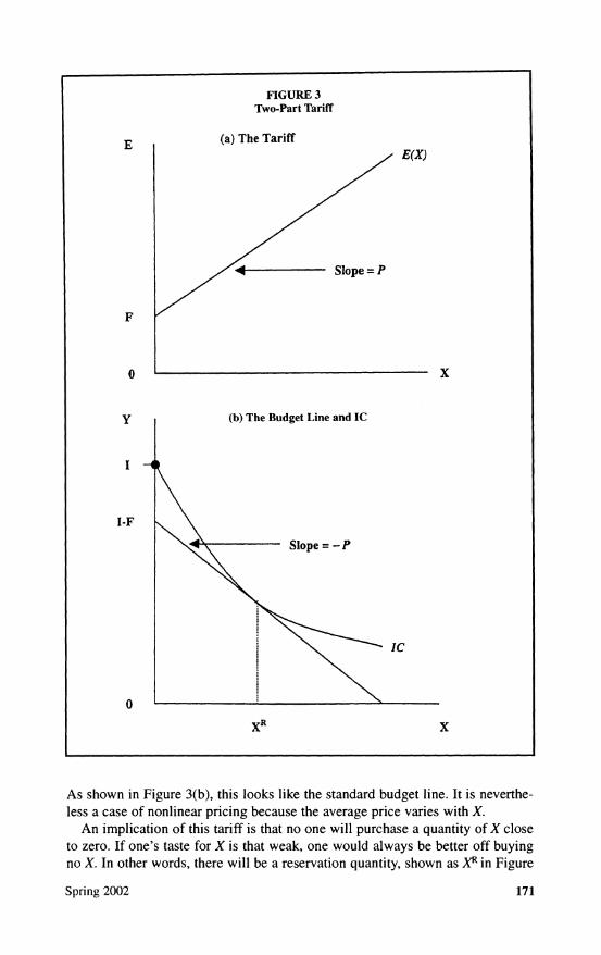
FIGURE 3 Two-Part Tariff

E (a) The Tariff E(X)

"- - Slope = P

F

o X

y (b) The Budget Line and IC

I -

I-F

Slope = -P

IC

0

XR x

As shown in Figure 3(b), this looks like the standard budget line. It is nevertheless a case of nonlinear pricing because the average price varies with X.

An implication of this tariff is that no one will purchase a quantity of X close to zero. If one's taste for X is that weak, one would always be better off buying no X. In other words, there will be a reservation quantity, shown as XR in Figure

Spring 2002 171

3(b). People will not buy from a discount store that requires an entry fee (e.g., Sam's Club) if the quantity to be purchased is too small.

Three-Part Tariff

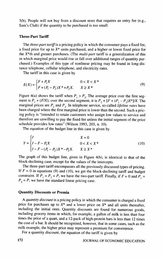
The three-part tariffis a pricing policy in which the consumer pays a fixed fee, a fixed price for up to X* units purchased, and a higher or lower fixed price for the X*th and greater purchases. (The multi-part tariff is a generalization of this in which marginal price would rise or fall over additional ranges of quantity purchased.) Examples of this type of nonlinear pricing may be found in long-dis- tance telephone, cellular telephone, and electricity rates.

The tariff in this case is given by

E(X) = FPx 0 < X < X (9) IF+(PI - P2)X*+P2X. X>2X*

Figure 4(a) shows the tariff when P, > P2. The average price over the first segment is P, + (FIX); over the second segment, it is P2 + [F + (P1 - P2)X*]/X. The marginal prices are P, and P2. In telephone service, so-called lifeline rates have been charged where the first marginal price is lower than the second. Such a pricing policy is "intended to retain customers who assign low values to service and therefore are unwilling to pay the fixed fee unless the initial segment of the price schedule provides low rates" (Wilson 1993, 203, n. 10).

The equation of the budget line in this case is given by

I X=0 Y= I-F-PIX 0<X<X* (10)

I- F-(P, -P2)X*-P2X. X>2X*

The graph of this budget line, given in Figure 4(b), is identical to that of the block-declining case, except for the values of the intercepts.

The three-part tariff encompasses all the previously discussed types of pricing. If F = 0 in equations (9) and (10), we get the block-declining tariff and budget constraint. If P1 = P2 = P, we have the two-part tariff. Finally, if F = 0 and P1

= P2 = P, we have the standard linear pricing case.

Quantity Discounts or Premia

A quantity discount is a pricing policy in which the consumer is charged a fixed price for purchases up to X* and a lower price on X* and all units thereafter, including the initial ones. Quantity discounts are found for numerous goods, including grocery items in which, for example, a gallon of milk is less than four times the price of a quart, and a 12-pack of high-protein bars is less than 12 times the cost of a bar. It should be recognized, however, that in some cases, such as the milk example, the higher price may represent a premium for convenience.

For a quantity discount, the equation of the tariff is given by


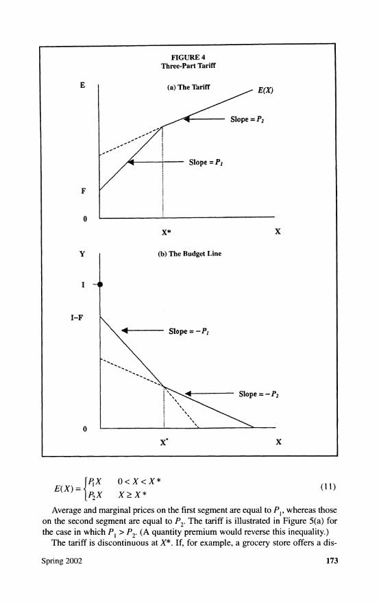
FIGURE 4 Three-Part Tariff

E (a) The Tariff E(X)

Slope = P2

SSlope = P,

F

0

X* X

Y (b) The Budget Line

I

I-F

Slope = - P

* - Slope=-P2

0

x x

RPiX O<X<X* E(X) = 1 O<X<X (11)

E P2X X

_ X *

Average and marginal prices on the first segment are equal to P,, whereas those on the second segment are equal to P2. The tariff is illustrated in Figure 5(a) for the case in which P, > P2. (A quantity premium would reverse this inequality.)

The tariff is discontinuous at X*. If, for example, a grocery store offers a dis-

Spring 2002 173

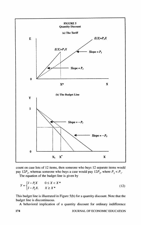
FIGURE 5 Quantity Discount

(a) The Tariff

E E(X)=P2X

E(X)=PIX ---X- Slope = P2

"I i- Slope = P,

0

X* X

(b) The Budget Line Y

I

, Slope = - P

SSlope = -P2

X X X1 X0x

count on case lots of 12 items, then someone who buys 12 separate items would

pay 12P,, whereas someone who buys a case would pay 12P2, where P2< Pl" The equation of the budget line is given by

I-PIX X<X*(12)

Y I - P2X. X >

X * (12)

This budget line is illustrated in Figure 5(b) for a quantity discount. Note that the budget line is discontinuous.

A behavioral implication of a quantity discount for ordinary indifference


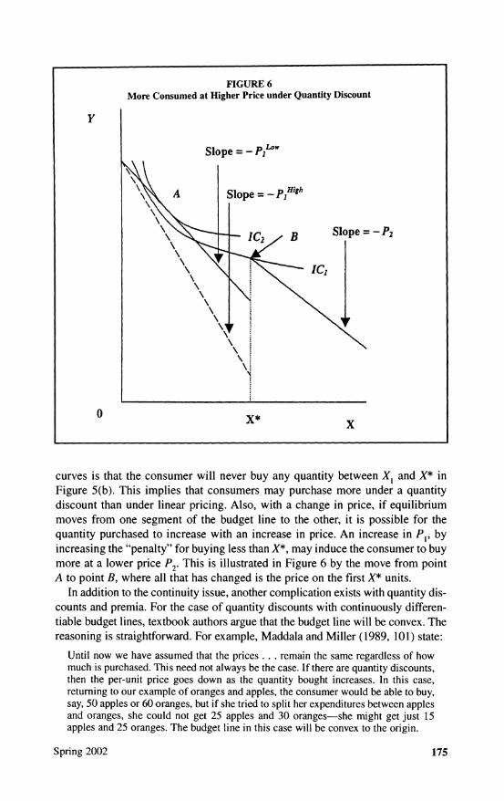
FIGURE 6 More Consumed at Higher Price under Quantity Discount

Y

Slope = - PLO'

• A Slope = - PHigh

IC2 B Slope = - P2

-c- B ,

0 x

curves is that the consumer will never buy any quantity between X, and X* in Figure 5(b). This implies that consumers may purchase more under a quantity discount than under linear pricing. Also, with a change in price, if equilibrium moves from one segment of the budget line to the other, it is possible for the quantity purchased to increase with an increase in price. An increase in P,, by increasing the "penalty" for buying less than X*, may induce the consumer to buy more at a lower price P2. This is illustrated in Figure 6 by the move from point A to point B, where all that has changed is the price on the first X* units.

In addition to the continuity issue, another complication exists with quantity discounts and premia. For the case of quantity discounts with continuously differentiable budget lines, textbook authors argue that the budget line will be convex. The reasoning is straightforward. For example, Maddala and Miller (1989, 101) state:

Until now we have assumed that the prices . . . remain the same regardless of how much is purchased. This need not always be the case. If there are quantity discounts, then the per-unit price goes down as the quantity bought increases. In this case, returning to our example of oranges and apples, the consumer would be able to buy, say, 50 apples or 60 oranges, but if she tried to split her expenditures between apples and oranges, she could not get 25 apples and 30 oranges-she might get just 15 apples and 25 oranges. The budget line in this case will be convex to the origin.

Spring 2002 175

Baumol (1977, 202-03) provides the only treatment we found of quantity premia, and he argues that the budget line is strictly concave in this case.4

Textbook authors who use piecewise linear budget constraints also assume the budget line is convex. The only exception we have found was Pashigian (1995, 56-57). His example involves a discount on every second unit purchased, that is, the second, fourth, and other even-numbered units, whereas the nondiscounted price applies to the odd-numbered units purchased. Although he does not discuss convexity or concavity in this context, his graph clearly shows a budget line that has both convex and concave segments. (In our terminology, this would not be a case of a quantity discount, however, but a multi-part tariff.)

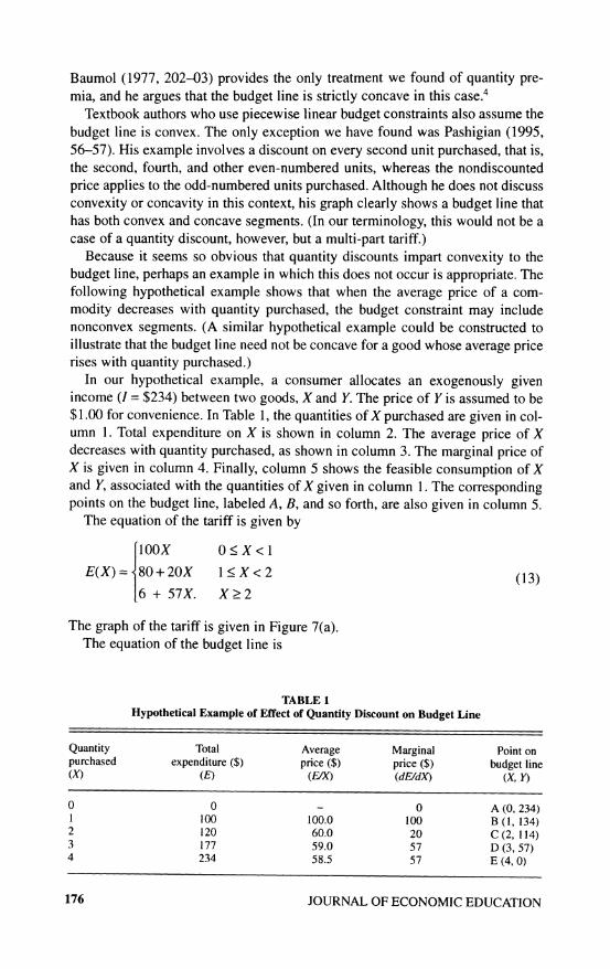
Because it seems so obvious that quantity discounts impart convexity to the budget line, perhaps an example in which this does not occur is appropriate. The following hypothetical example shows that when the average price of a commodity decreases with quantity purchased, the budget constraint may include nonconvex segments. (A similar hypothetical example could be constructed to illustrate that the budget line need not be concave for a good whose average price rises with quantity purchased.)

In our hypothetical example, a consumer allocates an exogenously given income (I = $234) between two goods, X and Y. The price of Y is assumed to be $1.00 for convenience. In Table 1, the quantities of X purchased are given in column 1. Total expenditure on X is shown in column 2. The average price of X decreases with quantity purchased, as shown in column 3. The marginal price of X is given in column 4. Finally, column 5 shows the feasible consumption of X and Y, associated with the quantities of X given in column 1. The corresponding points on the budget line, labeled A, B, and so forth, are also given in column 5.

The equation of the tariff is given by

10OX 0 < X < 1

E(X)= 80+ 20X 1 X < 2(13) 6 + 57X. X>2

The graph of the tariff is given in Figure 7(a). The equation of the budget line is

TABLE 1 Hypothetical Example of Effect of Quantity Discount on Budget Line

Quantity Total Average Marginal Point on purchased expenditure ($) price ($) price ($) budget line (X) (E) (EX) (dE/dX) (X, Y)

0 0 0 A (0, 234) 1 100 100.0 100 B (1, 134) 2 120 60.0 20 C (2, 114) 3 177 59.0 57 D (3, 57) 4 234 58.5 57 E (4, 0)


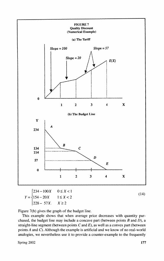
FIGURE 7 Quality Discount

(Numerical Example)

(a) The Tariff

Slope = 100 Slope = 57

Slope = 20E(X)

0

1 2 3 4 X

(b) The Budget Line

Y

A 234

B 134 ---- ... C 114

D 57 - -- - - - - - - -

E

1 2 3 4 X

234 - 100X 0 < X < 1

Y= 154- 20X 15X<2 (14) {228- 57X. X 2

Figure 7(b) gives the graph of the budget line. This example shows that when average price decreases with quantity pur-

chased, the budget line may include a concave part (between points B and D), a straight-line segment (between points C and E), as well as a convex part (between points A and C). Although the example is artificial and we know of no real-world analogies, we nevertheless use it to provide a counter-example to the frequently

Spring 2002 177

encountered assertion that the budget line will be convex under quantity discounts by showing that under such circumstances the budget line may contain concave, straight-line, and convex portions.

To develop rigorously the conditions under which budget lines may have these properties, we assume continuously differentiable tariffs and budget lines. Wil- son (1993, 145-46) notes that some multi-part tariffs can be approximated with continuous functions. In addition, some textbooks use such budget lines.

The equation of expenditure on X is

E(X) = P(X)X, (15)

which implies that E' = P'X + P and E" = 2P' + P"X. As discussed earlier, the curvature of the budget line depends on the sign of E", hence on the sign of 2P' + P"X. It is obvious that it will not be possible to determine the shape of the budget line from the sign of P' alone. For quantity discounts, when P' < 0 and P" > -(2P' / X), the budget line will be concave. For goods whose prices rise with quantity purchased, when P' > 0 and P" < (-2P' / X), the budget line will be convex to the origin. However, if the price changes at a constant rate (P" = 0), the budget line will be convex in the presence of quantity discounts or concave in the presence of quantity premia.5

The intuition behind this result is quite simple. E" is the rate of change in the marginal price, which determines the slope of the budget line, whereas P' is the rate of change in the average price (price discount or premium). When price changes at a variable rate (P" : 0), the sign of the change in the marginal price (E") is not in general the same as the sign of the change in the average price (P'). If the average price is decreasing, the marginal price may increase, decrease, or remain constant. (This is, of course, the same reasoning that underlies the more well-known relationship between average and marginal cost and between average and marginal product.)

CONCLUSION

We have distinguished linear and nonlinear pricing, derived and illustrated tariffs and budgets lines for various types of nonlinear pricing, and noted several behavioral results. We show that consumer choice theory may be easily extended to include nonlinear pricing and that the extension yields some interesting behavioral results. Two complications can occur, however, in the presentation of quantity discounts and premia. The first results from neglecting the discontinuity that quantity discounts or premia may impart to the tariff and the budget line. The second complication results from overlooking the possibility of nonconvex portions of the budget line for quantity discounts and nonconcave portions for quantity premia. If it is assumed that average price changes at a constant rate with X, then this complication is avoided.

Pedagogically, we think treatment of nonlinear pricing would enhance the student's understanding of the theory of consumer choice, as do other extensions of the theory customarily employed in textbooks. As a practical matter, treatment of nonlinear pricing is important because of the ubiquity of the phenomenon. In


addition, all of the nonlinear pricing schemes discussed, other than the two-part tariff, may be illustrated with identical budget-line graphs (with the assumption of continuity for quantity discounts and premia). The two-part tariff may be illustrated with the standard budget line. This permits an easy generalization not cur- rently exploited by textbook authors. Furthermore, although we have not pursued the issue, there is the possibility of applications of the same results to production theory, using the isocost-isoquant apparatus.

For these reasons, we recommend that microeconomics textbooks include an exposition of nonlinear pricing in the context of the theory of consumer choice. Except for the case of quantity discounts and premia in which average and marginal prices change continuously, the mathematics of nonlinear pricing is simple and could be taught in an intermediate-level course. Even at this level, the mathematics could be omitted and graphs relied upon for the presentation. The mathematics associated with continuously varying marginal and average price would go beyond the level of the intermediate microeconomics course, but it could be incorporated into a graduate microeconomics or a mathematical economics course, either as an exercise for the student or exposited in the text.

NOTES

1. The terminology relating to nonlinear pricing used here follows Wilson (1993). We shall use the terms tariff and total expenditures interchangeably in this article.

2. See Wilson (1993, 96), where he "construes nonlinear pricing as a particular kind of product dif- ferentiation. The product line comprises the various incremental units, each offered at its own price, plus possibly a minimal purchase.... This viewpoint is also illustrated by construing nonlinear pricing as a special case of bundling." Some textbook authors treat the block-declining tariff as a quantity discount (e.g., Nicholson 2000, 75). We reserve that term for a pricing scheme that offers a lower price on all units if a particular quantity is purchased.

3. Some textbook authors note this possibility (e.g., Nicholson 2000, 75). 4. A concave budget line is given as the answer to an exercise in Katz and Rosen (1998, 44, 623). 5. The analysis can easily be extended to the case in which both prices are variables. In that case, the

equation of the budget line is I = P(X)X + Pr(Y)Y, where P, is the price of good Y. The slope of the budget line is given by dY/dX = -[P'(X)X + P(X)]/[P'(Y)Y + P(Y)]. The curvature of the budget line is given by d2Y/dX2 = -[2P' + XP" + (2PY + YPr')(dY/dX)2]/(Pr + YFr), which depends on the signs of the changes in prices as well as the rates at which the prices are changing. Again, quantity discounts do not ensure the convexity of the budget line, and quantity premia do not ensure concavity.

REFERENCES

Baumol, W. J. 1977. Economic theory and operations analysis. 4th ed. Englewood Cliffs, N.J.: Pren- tice-Hall.

Browning, E. K., and M. A. Zupan. 1999. Microeconomic theory and applications. 6th ed. Reading, Mass.: Addison-Wesley Educational Publishers.

Katz, M. L., and H. S. Rosen. 1998. Microeconomics. 3rd ed. Boston, Mass.: Irwin/McGraw-Hill. Maddala, G. S., and E. Miller. 1989. Microeconomics. New York: McGraw-Hill. Moffitt, R. 1990. The econometrics of kinked budget constraints. Journal of Economic Perspectives

4 (2): 119-39. Nicholson, W. 2000. Intermediate microeconomics and its applications. 8th ed. Fort Worth, Tex.: Dryden. Oi, W. Y. 1971. A Disneyland dilemma: Two-part tariffs for a Mickey Mouse monopoly. Quarterly

Journal of Economics 85 (1): 77-96. Pashigian, B. P. 1995. Price theory and applications. New York: McGraw-Hill. Pindyck, R. S., and D. L. Rubinfeld. 1998. Microeconomics. 4th ed. Upper Saddle River, N.J.: Pren-

tice-Hall. Varian, H. R. 1999. Intermediate microeconomics: A modern approach. 5th ed. New York: W.W. Norton. Wilson, R. 1993. Nonlinear pricing. New York: Oxford University Press.

Spring 2002 179

introducing nonlinear pricing into consumer choice theoryeconomics.usf.edu/pdf/jee 33(2)...

Documents