introduction - american mathematical society · the conventional approach or nitsche’s technique....
TRANSCRIPT
MATHEMATICS OF COMPUTATIONVolume 78, Number 267, July 2009, Pages 1353–1374S 0025-5718(08)02183-2Article electronically published on September 25, 2008
NITSCHE’S METHOD FORGENERAL BOUNDARY CONDITIONS
MIKA JUNTUNEN AND ROLF STENBERG
Abstract. We introduce a method for treating general boundary conditionsin the finite element method generalizing an approach, due to Nitsche (1971),for approximating Dirichlet boundary conditions. We use Poisson’s equationsas a model problem and prove a priori and a posteriori error estimates. Themethod is also compared with the traditional Galerkin method. The theoreti-cal results are verified numerically.
1. Introduction
In his classical paper [6] Nitsche discusses techniques for incorporating Dirich-let boundary conditions in the finite element approximation of the model Poissonproblem: find u such that
−∆u = f in Ω,(1.1)
u = u0 on Γ = ∂Ω.(1.2)
Before introducing his technique he discusses the penalty method, i.e. the Ritz ap-proximation to the “perturbed” problem in which the Dirichlet boundary condition(1.2) is replaced by the condition
(1.3)∂u
∂n=
1ε(u0 − u) on Γ,
where ε > 0 is a small parameter. He points out the drawbacks of this approach, i.e.nonconformity, which requires a coupling of the penalty parameter to the mesh size,and the possible ill-conditioning of the discrete system when the penalty parameteris too small (see [2] for a recent survey on this).
If instead of the Dirichlet problem we consider the problem with the boundarycondition (1.3), then the solution to the continuous problem converges to the so-lution of the Dirichlet problem when ε → 0. For the finite element discretizationthe discrete problem gets more ill-conditioned when ε approaches zero. In the limitε = 0, we have to switch to some other way of imposing the Dirichlet condition, likethe conventional approach or Nitsche’s technique. The following question arisesquite naturally: can we extend Nitsche’s method so that it can be used for thewhole range of boundary conditions ε ≥ 0 ? The purpose of this paper is to give a
Received by the editor October 17, 2007, and, in revised form, May 21, 2008.2000 Mathematics Subject Classification. Primary 65N30.This work was supported by the Finnish National Graduate School in Engineering Mechanics,
by the Academy of Finland, and TEKES, the National Technology Agency of Finland.
c©2008 American Mathematical Society
1353
License or copyright restrictions may apply to redistribution; see https://www.ams.org/journal-terms-of-use

1354 MIKA JUNTUNEN AND ROLF STENBERG
positive answer to this question. We will consider general boundary conditions andextend Nitsche’s method to cover the whole class of problems.
The outline of the paper is as follows. In the next section we derive the methodand show that it is consistent. In Section 3 we prove the ellipticity and derive thea priori error estimates. Section 4 is devoted to the a posteriori error estimates.For the a posteriori estimate we show that it gives both an upper bound and alower bound to the error. In Section 5 we give a summary of the error analysisof the traditional finite element method. Finally, in Section 6, we show numericalapplications of the proposed method and the error estimates and compare them tothose obtained with the traditional method.
2. The method and its consistency
We consider the following problem:
−∆u = f in Ω,(2.1)∂u
∂n=
1ε(u0 − u) + g on Γ,(2.2)
where Ω is a bounded domain with polygonal boundary, f ∈ L2(Ω), u0 ∈ H1/2(Γ),g ∈ L2(Γ) and ε ∈ R, 0 ≤ ε ≤ ∞. The limiting values of the parameter ε give thepure Dirichlet and Neumann problems, respectively, i.e.
(2.3) ε → 0 ⇒ u = u0 on Γ, ε → ∞ ⇒ ∂u
∂n= g on Γ.
For simplicity we consider a shape regular finite element partitioning Th of thedomain Ω ⊂ R
N , N = 2, 3, into simplices, i.e. triangles or tetrahedra. Thispartitioning induces a mesh, denoted by Gh, on the boundary Γ. By K ∈ Th wedenote an element of the mesh and by E we denote one edge or face in Gh. By hK
we denote the diameter of the element K ∈ Th and by hE we denote the diameterof E ∈ Gh. We also define
h := maxhK : K ∈ Th
andVh := v ∈ H1(Ω) : v|K ∈ Pp(K) ∀K ∈ Th,
where Pp(K) is the space of polynomials of degree p. The method is now definedas follows. Here γ is a positive parameter that has to be bounded from above; seeTheorem 3.2 below.
Nitsche’s method. Find uh ∈ Vh such that
(2.4) Bh(uh, v) = Fh(v) ∀v ∈ Vh,
where
(2.5) Bh(u, v) =(∇u,∇v
)Ω
+∑
E∈Gh
− γhE
ε + γhE
[ ⟨∂u
∂n, v
⟩E
+⟨u,
∂v
∂n
⟩E
]
+1
ε + γhE
⟨u, v
⟩E− εγhE
ε + γhE
⟨∂u
∂n,∂v
∂n
⟩E
License or copyright restrictions may apply to redistribution; see https://www.ams.org/journal-terms-of-use

NITSCHE’S METHOD FOR GENERAL BOUNDARY CONDITIONS 1355
and
(2.6) Fh(v) =(f, v
)Ω
+∑
E∈Gh
1
ε + γhE
⟨u0, v
⟩E− γhE
ε + γhE
⟨u0,
∂v
∂n
⟩E
+ε
ε + γhE
⟨g, v
⟩E− εγhE
ε + γhE
⟨g,
∂v
∂n
⟩E
.
Next we prove the consistency of the proposed method.
Lemma 2.1. The solution u of the equations (2.1)–(2.2) satisfies
(2.7) Bh(u, v) = Fh(v) ∀v ∈ Vh.
Proof. Multiplying the differential equation (2.1) with v ∈ Vh, integrating over thedomain Ω, and using Green’s formula leads to
(2.8)(∇u,∇v
)Ω−
⟨∂u
∂n, v
⟩Γ
=(f, v
)Ω.
Next, multiplying the boundary condition (2.2) by v, and integrating over an ele-ment E, we have
(2.9) ε⟨∂u
∂n, v
⟩E
+⟨u, v
⟩E
=⟨u0, v
⟩E
+ ε⟨g, v
⟩E
.
This gives(2.10)∑
E∈Gh
1ε + γhE
ε⟨∂u
∂n, v
⟩E
+⟨u, v
⟩E
=
∑E∈Gh
1ε + γhE
⟨u0, v
⟩E
+ ε⟨g, v
⟩E
.
Similarly, we obtain
(2.11)
∑E∈Gh
− γhE
ε + γhE
ε⟨∂u
∂n,∂v
∂n
⟩E
+⟨u,
∂v
∂n
⟩E
=∑
E∈Gh
− γhE
ε + γhE
⟨u0,
∂v
∂n
⟩E
+ ε⟨g,
∂v
∂n
⟩E
.
The equation (2.7) is now the sum of equations (2.8), (2.10), and (2.11). The method has two parameters, the stability parameter γ and the problem
dependent parameter ε in the boundary condition. By choosing γ = 0 in (2.4) weget:
The traditional method. Find uh ∈ Vh such that
(2.12)(∇uh,∇v
)Ω
+1ε
⟨uh, v
⟩Γ
=(f, v
)Ω
+1ε
⟨u0, v
⟩Γ
+⟨g, v
⟩Γ
∀v ∈ Vh.
This may become ill-conditioned when ε > 0 is small. We will return to this methodin Section 5 below.
For the stabilized method with γ > 0 we obtain, in the limit ε = 0,
(2.13)
(∇uh,∇v
)Ω−
⟨∂uh
∂n, v
⟩Γ−
⟨uh,
∂v
∂n
⟩Γ
+∑
E∈Gh
1γhE
⟨uh, v
⟩E
=(f, v
)Ω−
⟨u0,
∂v
∂n
⟩Γ
+∑
E∈Gh
1γhE
⟨u0, v
⟩E
∀v ∈ Vh,
License or copyright restrictions may apply to redistribution; see https://www.ams.org/journal-terms-of-use
1356 MIKA JUNTUNEN AND ROLF STENBERG
which is Nitsche’s method [7] applied to the Dirichlet problem
−∆u = f in Ω,
u = u0 on Γ.
This is also exactly how the Dirichlet boundary conditions are treated in the InteriorPenalty Discontinuous Galerkin method; cf. [1].
When ε → ∞ the problem to be solved is the pure Neumann problem
−∆u = f in Ω,
∂u
∂n= g on Γ,
which is approximated by
(2.14)
(∇uh,∇v
)Ω−
∑E∈Gh
γhE
⟨∂uh
∂n,∂v
∂n
⟩E
=(f, v
)Ω
+⟨g, v
⟩Γ−
∑E∈Gh
γhE
⟨g,
∂v
∂n
⟩E
.
This is the variational form of the Neumann problem with the extra terms
−∑
E∈Gh
γhE
⟨∂uh
∂n,∂v
∂n
⟩E
and −∑
E∈Gh
γhE
⟨g,
∂v
∂n
⟩E
,
which do not affect the consistency of the method. Note, that the Neumann problemrequires that the data satisfy
(2.15)(f, 1
)Ω
+⟨g, 1
⟩Γ
= 0,
and this condition is not violated in our formulation.
3. Stability and a priori error estimates
In the stability and error analysis we will use the following mesh-dependentnorms
(3.1) ‖v‖2h := ‖∇v‖2
L2(Ω) +∑
E∈Gh
1ε + hE
‖v‖2L2(E)
and
(3.2) |‖v‖|2h := ‖v‖2h +
∑E∈Gh
hE
∥∥∥∥ ∂v
∂n
∥∥∥∥2
L2(E)
.
In the subspace Vh these two norms are equivalent. This follows from the well-known estimate below.
Lemma 3.1. There is a positive constant CI such that
(3.3)∑
E∈Gh
hE
∥∥∥∥ ∂v
∂n
∥∥∥∥2
L2(E)
≤ CI‖∇v‖2L2(Ω) ∀v ∈ Vh.
For the formulation we have the following stability result. Here and in what fol-lows, C denotes a generic positive constant independent of both the mesh parameterh and the parameter ε.
License or copyright restrictions may apply to redistribution; see https://www.ams.org/journal-terms-of-use
NITSCHE’S METHOD FOR GENERAL BOUNDARY CONDITIONS 1357
Theorem 3.2. Suppose that 0 < γ < 1/CI . Then there exists a positive constantC such that
(3.4) Bh(v, v) ≥ C‖v‖2h ∀v ∈ Vh.
Proof. First, the Schwarz inequality gives
(3.5)
Bh(v, v) =(∇v,∇v
)Ω
+∑
E∈Gh
− γhE
ε + γhE
[ ⟨∂v
∂n, v
⟩E
+⟨v,
∂v
∂n
⟩E
]
+1
ε + γhE
⟨v, v
⟩E− εγhE
ε + γhE
⟨ ∂v
∂n,∂v
∂n
⟩E
≥ ‖∇v‖2L2(Ω) +
∑E∈Gh
− 2
γhE
ε + γhE
∥∥∥∥ ∂v
∂n
∥∥∥∥L2(E)
‖v‖L2(E)
+1
ε + γhE‖v‖2
L2(E) −εγhE
ε + γhE
∥∥∥∥ ∂v
∂n
∥∥∥∥2
L2(E)
.
Next, using Young’s inequality, with δ > 0, we get(3.6)
Bh(v, v) ≥(
1 − 1δ
CIγ2hE
ε + γhE− CIεγ
ε + γhE
)‖∇v‖2
L2(Ω) + C1 − δ
ε + γhE‖v‖2
L2(Γ).
The second term is positive if 1 − δ > 0 and the first term is positive if(3.7)
1 − 1δ
CIγ2hE
ε + γhE− CIεγ
ε + γhE=
1ε + γhE
(ε (1 − CIγ) + γhE
(1 − CIγ
δ
))> 0.
Hence, we choose δ such that CIγ < δ < 1. The choice is possible due to theassumption γ < 1/CI . This shows that Bh(v, v) ≥ C‖v‖2
h with C > 0 independentof ε and h.
In the rest of the paper we will assume that the stability requirement is satisfied,i.e. we make the following assumption.
Assumption 3.3. The real parameter γ satisfies 0 < γ < CI .
For the a priori estimate we need the following well-known interpolation estimate.
Lemma 3.4. Suppose that u ∈ Hs(Ω), with 3/2 < s ≤ p + 1. Then it holds that
(3.8) infv∈Vh
|||u − v|||h ≤ Chs−1‖u‖Hs(Ω).
We then have
Theorem 3.5. For u ∈ Hs(Ω), with 3/2 < s ≤ p + 1 it holds that
(3.9) ‖u − uh‖h ≤ Chs−1‖u‖Hs(Ω).
Proof. From the consistency and coercivity, i.e. Lemma 2.1 and Theorem 3.2, weget
(3.10) ‖uh − v‖2h ≤ CBh(uh − v, uh − v) ≤ CBh(u − v, uh − v) ∀v ∈ Vh.
Using the continuity of the bilinear form and the two norms ‖ · ‖h and |‖ · |‖h wehave the bound
(3.11) Bh(u − v, uh − v) ≤ C|||u − v|||h‖uh − v‖h ∀v ∈ Vh.
License or copyright restrictions may apply to redistribution; see https://www.ams.org/journal-terms-of-use
1358 MIKA JUNTUNEN AND ROLF STENBERG
Combining equations (3.10) and (3.11) we have
(3.12) ‖uh − v‖h ≤ C|||u − v|||h ∀v ∈ Vh
and the assertion follows by triangle inequality and Lemma 3.4 above.
4. A posteriori error estimate
In this section we introduce a residual based a posteriori error estimator for theproblem. We will prove that this gives both an upper and a lower bound for theerror.
For the proof we will use a mesh Th/2 obtained from Th by dividing each simplexinto 2N , N = 2, 3, equal simplices. The corresponding mesh induced on Γ will bedenoted by Gh/2. By Vh/2 we denote the finite element subspace on the refinedmesh and uh/2 ∈ Vh/2 is the corresponding finite element solution. By Ih andIh/2 we denote the collection of interior edges/faces of elements in Th and Th/2,respectively.
The local error indicator is defined as
(4.1)
EK(uh)2 = h2K‖∆uh + f‖2
L2(K) + hE
∥∥∥∥[[∂uh
∂n
]]∥∥∥∥2
L2(∂K∩Ih)
+hE
(ε + γhE)2
∥∥∥∥ε(∂uh
∂n− g
)+ uh − u0
∥∥∥∥2
L2(∂K∩Γ)
.
In our analysis we use the following saturation assumption [4].
Assumption 4.1. Assume there exists β < 1 such that
(4.2) ‖u − uh/2‖h/2 ≤ β‖u − uh‖h,
where uh/2 is the solution on the mesh Th/2. The mesh Th/2 is derived by splittingthe elements of the mesh Th.
We then have the following result.
Theorem 4.2. Under the Assumptions 3.3 and 4.1 it holds that
(4.3) ‖u − uh‖h ≤ C( ∑
K∈Th
EK(uh)2)1/2
.
Proof. Step 1. By the triangle inequality we have
(4.4) ‖uh/2 − uh‖h/2 ≥ ‖u − uh‖h/2 − ‖u − uh/2‖h/2 ≥ ‖u − uh‖h − β‖u − uh‖h
and as a consequence of the saturation assumption we have
(4.5) ‖u − uh‖h ≤ 11 − β
‖uh/2 − uh‖h/2.
Hence, it is sufficient to bound ‖uh/2−uh‖h/2. To this end we use the stability. ByTheorem 3.2 there exists v ∈ Vh/2 such that
(4.6) ‖v‖h/2 = 1 and C‖uh/2 − uh‖h/2 ≤ Bh/2(uh/2 − uh, v).
License or copyright restrictions may apply to redistribution; see https://www.ams.org/journal-terms-of-use

NITSCHE’S METHOD FOR GENERAL BOUNDARY CONDITIONS 1359
Let v ∈ Vh be the Lagrange interpolate of v ∈ Vh/2. By scaling arguments oneobtains
(4.7)
∑K∈Th/2
h−2
K ‖v − v‖2L2(K) + h−1
E ‖v − v‖2L2(∂K)
+∑
E∈Gh/2
1ε + hE
‖v − v‖2L2(E) + hE‖
∂(v − v)∂n
‖2L2(E)
≤ C‖v‖2h/2 ≤ C.
To simplify the notation we define w := v − v and the above estimate gives
(4.8)
( ∑K∈Th/2
h−2K ‖w‖2
L2(K)
)1/2
≤ C,( ∑
K∈Th/2
h−1E ‖w‖2
L2(∂K)
)1/2
≤ C
and( ∑
E∈Gh/2
hE‖∂w
∂n‖2
L2(E)
)1/2
≤ C.
In (4.6) we split the right-hand side into two parts:
(4.9) Bh/2(uh/2 − uh, v) ≤ Bh/2(uh/2 − uh, w) + Bh/2(uh/2 − uh, v) =: W1 + W2.
We will bound the terms W1 and W2 separately.Step 2. Since w ∈ Vh/2, it holds that
(4.10) Bh/2(uh/2, w) = Fh/2(w),
and we have
(4.11)
W1 = Fh/2(w) − Bh/2(uh, w)
=
(f, w
)Ω−
(∇uh,∇w
)Ω
+∑
E∈Gh/2
γhE
ε + γhE
⟨∂uh
∂n, w
⟩E
+∑
E∈Gh/2
1ε + γhE
[⟨u0 − uh, w
⟩E
+ ε⟨g, w
⟩E
]
+∑
E∈Gh/2
γhE
ε + γhE
[⟨uh − u0,
∂w
∂n
⟩E
+ ε⟨∂uh
∂n− g,
∂w
∂n
⟩E
].
Integrating by parts on each K ∈ Th/2 gives
(4.12)
(f, w
)Ω−
(∇uh,∇w
)Ω
=∑
K∈Th/2
(f + ∆uh, w
)K−
∑E∈Ih/2
⟨[[∂uh
∂n
]], w
⟩E
−∑
E∈Gh/2
⟨∂uh
∂n, w
⟩E
.
Rearranging terms we thus have
(4.13) W1 = R1 + R2 + R3,
License or copyright restrictions may apply to redistribution; see https://www.ams.org/journal-terms-of-use

1360 MIKA JUNTUNEN AND ROLF STENBERG
with
R1 =∑
K∈Th/2
(f + ∆uh, w
)K−
∑E∈Ih/2
⟨[[∂uh
∂n
]], w
⟩E
,(4.14)
R2 =∑
E∈Gh/2
( γhE
ε + γhE− 1
)⟨∂uh
∂n, w
⟩E
(4.15)
+∑
E∈Gh/2
1ε + γhE
[⟨u0 − uh, w
⟩E
+ ε⟨g, w
⟩E
],
and
(4.16) R3 =∑
E∈Gh/2
γhE
ε + γhE
[⟨uh − u0,
∂w
∂n
⟩E
+ ε⟨∂uh
∂n− g,
∂w
∂n
⟩E
].
The first term is estimated using Schwarz inequality and (4.8)(4.17)
R1 ≤∑
K∈Th/2
∥∥f + ∆uh
∥∥L2(K)
∥∥w∥∥
L2(K)+
∑E∈Ih/2
∥∥∥[[∂uh
∂n
]]∥∥∥L2(E)
∥∥w∥∥
L2(E)
≤( ∑
K∈Th/2
h2K
∥∥f + ∆uh
∥∥L2(K)
)1/2( ∑K∈Th/2
h−2K
∥∥w∥∥
L2(K)
)1/2
+( ∑
E∈Ih/2
hE
∥∥∥[[∂uh
∂n
]]∥∥∥L2(E)
)1/2( ∑E∈Ih/2
h−1E
∥∥w∥∥
L2(E)
)1/2
≤ C[( ∑
K∈Th/2
h2K
∥∥f + ∆uh
∥∥L2(K)
)1/2
+( ∑
E∈Ih/2
hE
∥∥∥[[∂uh
∂n
]]∥∥∥L2(E)
)1/2].
Adding the terms in R2, using Schwarz inequality and the estimate (4.8) gives
(4.18)
R2 =∑
E∈Gh/2
1ε + γhE
⟨u0 − uh + εg − ε
∂uh
∂n, w
⟩E
≤( ∑
E∈Gh/2
hE
(ε + γhE)2
∥∥∥∥uh − u0 + ε(∂uh
∂n− g
)∥∥∥∥2
L2(E)
)1/2
·( ∑
E∈Gh/2
h−1E ‖w‖2
L2(E)
)1/2
≤ C( ∑
E∈Gh/2
hE
(ε + γhE)2
∥∥∥∥uh − u0 + ε(∂uh
∂n− g
)∥∥∥∥2
L2(E)
)1/2
.
License or copyright restrictions may apply to redistribution; see https://www.ams.org/journal-terms-of-use
NITSCHE’S METHOD FOR GENERAL BOUNDARY CONDITIONS 1361
For the third term we similarly get
(4.19)
R3 =∑
E∈Gh/2
γhE
ε + γhE
[⟨uh − u0 + ε(
∂uh
∂n− g),
∂w
∂n
⟩E
]
≤ γ
( ∑E∈Gh/2
hE
(ε + γhE)2
∥∥∥⟨uh − u0 + ε(
∂uh
∂n− g)
∥∥∥2)1/2
·( ∑
E∈Gh/2
hE
∥∥∥∂w
∂n
∥∥∥2
E
)1/2
≤ C
( ∑E∈Gh/2
hE
(ε + γhE)2
∥∥∥⟨uh − u0 + ε(
∂uh
∂n− g)
∥∥∥2)1/2
.
Now we have bounded the term W1, i.e. we have
(4.20) W1 ≤ C( ∑
K∈Th/2
EK(uh)2)1/2
.
Step 3. Next, we prove the same upper bound to term W2 of equation (4.9). Toobtain the upper bound we need the following bounds:
(4.21) ‖v‖h/2 +( ∑
E∈Gh/2
hE
∥∥∥∥∂v
∂n
∥∥∥∥2
L2(E)
)1/2
≤ C‖v‖h/2 ≤ C,
which follow from (4.7) and (4.6). Below, for clarity, we will denote by E an elementin Gh/2 and by F an element in Gh. Using the relation Bh(uh, v) − Fh(v) = 0 andrearranging terms we obtain
(4.22)
W2 = Fh/2(v) − Bh/2(uh, v) = Fh/2(v) −Fh(v) + Bh(uh, v) − Bh/2(uh, v)
=
⎡⎣ ∑
E∈Gh/2
1ε + γhE
⟨u0 − uh + εg, v
⟩E
⎤⎦
+
[−
∑F∈Gh
1ε + γhF
⟨u0 − uh + εg, v
⟩F
]
+
⎡⎣ ∑
E∈Gh/2
γhE
ε + γhE
⟨∂uh
∂n, v
⟩E−
∑F∈Gh
γhF
ε + γhF
⟨∂uh
∂n, v
⟩F
⎤⎦
+
⎡⎣ ∑
E∈Gh/2
γhE
ε + γhE
⟨uh − u0 + ε(
∂uh
∂n− g),
∂v
∂n
⟩E
⎤⎦
+
[−
∑F∈Gh
γhF
ε + γhF
⟨uh − u0 + ε(
∂uh
∂n− g),
∂v
∂n
⟩F
]
= T1 + T2 + T3 + T4 + T5.
License or copyright restrictions may apply to redistribution; see https://www.ams.org/journal-terms-of-use
1362 MIKA JUNTUNEN AND ROLF STENBERG
Since uh has the same values on both meshes Th/2 and Th, we can write the termT3 as follows:
(4.23)
T3 =
⎡⎣ ∑
E∈Gh/2
γhE
ε + γhE
⟨∂uh
∂n, v
⟩E−
∑F∈Gh
γhF
ε + γhF
⟨∂uh
∂n, v
⟩F
⎤⎦
=
⎡⎣ ∑
E∈Gh/2
( γhE
ε + γhE− 1
)⟨∂uh
∂n, v
⟩E−
∑F∈Gh
( γhF
ε + γhF− 1
)⟨∂uh
∂n, v
⟩F
⎤⎦
= −∑
E∈Gh/2
ε
ε + γhE
⟨∂uh
∂n, v
⟩E
+∑
F∈Gh
ε
ε + γhF
⟨∂uh
∂n, v
⟩F.
Next, adding T1, T2 and T3, and using the fact that hF = 2hE, for E ⊂ F , gives
(4.24)
T1 + T2 + T3 =∑
E∈Gh/2
1ε + γhE
⟨u0 − uh + ε
(g − ∂uh
∂n
), v
⟩E
−∑
F∈Gh
1ε + γhF
⟨u0 − uh + ε
(g − ∂uh
∂n
), v
⟩F
=∑
E∈Gh/2
γhE
(ε + γhE)(ε + 2γhE)⟨u0 − uh + ε
(g − ∂uh
∂n
), v
⟩E
≤ C∑
E∈Gh/2
hE
(ε + γhE)3/2
∥∥∥∥uh − u0 + ε(∂uh
∂n− g)
∥∥∥∥L2(E)
· 1(ε + γhE)1/2
‖v‖L2(E)
≤ C
( ∑E∈Gh/2
h2E
(ε + γhE)3
∥∥∥∥uh − u0 + ε(∂uh
∂n− g)
∥∥∥∥2
L2(E)
)1/2
‖v‖h
≤ C
( ∑E∈Gh/2
hE
(ε + γhE)2
∥∥∥∥uh − u0 + ε(∂uh
∂n− g)
∥∥∥∥2
L2(E)
)1/2
.
The terms T4 and T5 of the equation (4.22) are the same terms on different meshesand the proofs are exactly the same for both of them. For brevity we show theproof only for T4
(4.25)
T4 ≤ C∑
E∈Gh/2
hE h−1/2E
ε + γhE
∥∥∥∥uh − u0 + ε(∂uh
∂n− g)
∥∥∥∥L2(E)
h1/2E
∥∥∥∥ ∂v
∂n
∥∥∥∥L2(E)
≤ C
( ∑E∈Gh/2
γhE
(ε + γhE)2
∥∥∥∥uh − u0 + ε(∂uh
∂n− g)
∥∥∥∥2
L2(E)
)1/2
·( ∑
E∈Gh/2
hE
∥∥∥∥ ∂v
∂n
∥∥∥∥2
L2(E)
)1/2
≤ C
( ∑E∈Gh/2
hE
(ε + γhE)2
∥∥∥∥uh − u0 + ε(∂uh
∂n− g)
∥∥∥∥2
L2(E)
)1/2
,
License or copyright restrictions may apply to redistribution; see https://www.ams.org/journal-terms-of-use

NITSCHE’S METHOD FOR GENERAL BOUNDARY CONDITIONS 1363
where last line follows from the bound of the interpolant; see equation (4.21). ForT5 we get
(4.26) T5 ≤ C
( ∑F∈Gh
hF
(ε + γhF )2
∥∥∥∥uh − u0 + ε(∂uh
∂n− g)
∥∥∥∥2
L2(F )
)1/2
.
Now we have also bounded the term W2, i.e. we have
(4.27) W2 ≤ C[( ∑
K∈Th/2
EK(uh)2)1/2
+( ∑
K∈Th
EK(uh)2)1/2]
.
Since uh ∈ Vh has the same values on both Th/2 and Th we have
(4.28)∑
K∈Th/2
EK(uh)2 ≤ C∑
K∈Th
EK(uh)2.
The assertion now follows by combining (4.5), (4.6), (4.9), (4.20) and (4.27).Let us next discuss the estimator. When ε = 0, i.e. for the pure Dirichlet
problem, we get
(4.29)
EK(uh)2 = h2K‖∆uh + f‖2
L2(K) +∑
E⊂∂K∩Ih
hE
∥∥∥∥[[∂uh
∂n
]]∥∥∥∥2
L2(E)
+∑
E⊂∂K∩Γ
1hE
‖uh − u0‖2L2(E) ,
which is the estimator of Nitsche’s method for the Dirichlet boundary value prob-lem; see [3]. Note also that the error is measured in the norm
(4.30) ‖v‖2h = ‖∇v‖2
L2(Ω) +∑
E∈Gh
1hE
‖v‖2L2(E).
The other limit, ε → ∞, leads to
(4.31)
EK(uh)2 = h2K‖∆uh + f‖2
L2(K) +∑
E⊂∂K∩Ih
hE
∥∥∥∥[[∂uh
∂n
]]∥∥∥∥2
L2(E)
+∑
E⊂∂K∩Γ
hE
∥∥∥∥∂uh
∂n− g
∥∥∥∥2
L2(E)
,
which is the traditional a posteriori estimator of the Neumann problem with theerror measured in the H1(Ω)-seminorm
(4.32) ‖v‖2h = ‖∇v‖2
L2(Ω).
These remarks show that the a posteriori estimate holds for all values of the pa-rameter ε, even the limit values give the correct and numerically stable a posterioriestimate.
Finally, we prove the efficiency of the a posteriori estimate. For the proof weuse and adopt established techniques using test functions with local support. Welet ΨE be the N -th degree polynomial which has the support ωE on the elementwith E as an edge/face and is normalized such that 0 ≤ ΨE ≤ 1 = maxΨE . Forthe edges we also need an extension operator E from the edge E to the elementssharing E, i.e.
E : L2(E) → L2(ωE).
License or copyright restrictions may apply to redistribution; see https://www.ams.org/journal-terms-of-use

1364 MIKA JUNTUNEN AND ROLF STENBERG
On the boundary ∂Ω we assume that ΨE and E operate in the obvious way, i.e.they only extend towards the interior of the domain Ω. For the bubble functionsand the extension operator the following estimates hold; see e.g. [8].
Lemma 4.3. Let Th be a shape-regular mesh. Then there exists C > 0 such that
‖Ψ1/2E pE‖L(E) ≥ C‖pE‖L2(E),(4.33)
Ch1/2K ‖pE‖L2(E) ≤ ‖ΨEEpE‖L2(K) ≤ Ch
1/2K ‖pE‖L2(E),(4.34)
‖∇(ΨEEpE)‖L2(K) ≤ Ch−1K ‖ΨEEpE‖L2(K),(4.35)
for all pE ∈ Pp(E), K ∈ Th and E ⊂ ∂K.
We now have the following local bounds.
Theorem 4.4. The elementwise estimator EK(uh), defined in equation (4.1), alsofulfills
(4.36)
EK(uh)2 ≤ C(|u−uh|2H1(ωK) +h2
K‖f −fh‖2L2(ωK) +
∑E⊂∂K∩Γ
1ε + hE
‖u−uh‖2L2(E)
+∑
E⊂∂K∩Γ
hE
(ε + hE)2‖ε(g − gh) + u0 − u0,h‖2
L2(E)
),
where fh, u0,h and gh are approximations in Vh of the given data, and ωK is thedomain of element K and all elements sharing an edge/face with K.
Proof. We will consider the upper bound for each term of the estimator EK(uh),equation (4.1), separately.
For the terms RK := ∆uh + f and RE := [[∂uh
∂n ]] we have the well-knownbounds [8]:
(4.37) hK‖RK‖L2(ωK) ≤ C(|u − uh|H1(ωK) + hK‖f − fh‖L2(ωK)
)and
(4.38) h1/2E ‖ RE‖L2(E) ≤ C
(|u − uh|H1(ωE) + hK‖ f − fh‖L2(ωE)
).
Therefore, we only give the proof for the last term
(4.39) RΓ = ε(∂uh
∂n− g) + uh − u0.
We denote
RΓ,red = ε(∂uh
∂n− gh) + uh − u0,h, wΓ = ΨEERΓ,red and wΓ = ΨERΓ,red.
With the triangle inequality we get
(4.40) ‖RΓ‖L2(E) ≤ ‖RΓ,red‖L2(E) + ‖ε(g − gh) + u0 − u0,h‖L2(E).
Lemma 4.3 and the identities(RK , wΓ
)K
=(∇(u − uh),∇wΓ
)K
+⟨ ∂
∂n(uh − u), wΓ
⟩E
,
and
ε(∂u
∂n− g) + (u0 − u) = 0,
License or copyright restrictions may apply to redistribution; see https://www.ams.org/journal-terms-of-use
NITSCHE’S METHOD FOR GENERAL BOUNDARY CONDITIONS 1365
lead to
(4.41)
C‖RΓ,red‖2L2(E) ≤ ‖Ψ1/2
E RΓ,red‖2L2(E) =
⟨RΓ,red, wΓ
⟩E
= ε⟨ ∂
∂n(uh − u), wΓ
⟩E
+⟨uh − u, wΓ
⟩E
+⟨ε(g − gh) + u0 − u0,h, wΓ
⟩E
= ε(RK , wΓ
)K
+ ε(∇(uh − u),∇wΓ
)K
+⟨uh − u, wΓ
⟩E
+⟨ε(g − gh) + u0 − u0,h, wΓ
⟩E
≤ ε‖RK‖L2(K)‖ wΓ‖L2(K) + ε‖ ∇(u − uh)‖L2(K)‖∇wΓ‖L2(K)
+ ‖uh − u‖L2(E)‖wΓ‖L2(E) + ‖ε(g − gh) + u0 − u0,h‖L2(E)‖wΓ‖L2(E)
≤ C(εh
1/2K ‖RK‖L2(K) + εh
−1/2K |u − uh|H1(K) + ‖u − uh‖L2(E)
+ ‖ε(g − gh) + u0 − u0,h‖L2(E)
)‖RΓ,red‖L2(E).
Multiplying equation (4.41) with h1/2E
ε+hEand using the bound (4.37) for ‖RK‖L2(K)
gives
(4.42)
h1/2E
ε + hE‖RΓ,red‖L2(E)
≤ C( ε
ε + hE|u − uh|H1(K) +
εhE
ε + hE‖f − fh‖L2(K)
+h
1/2E
ε + hE‖u − uh‖L2(E) +
h1/2E
ε + hE‖ε(g − gh) + u0 − u0,h‖L2(E)
)≤ C
(|u − uh|H1(K) + hK‖f − fh‖L2(K)
+1
(ε + hE)1/2‖u − uh‖L2(E) +
h1/2E
ε + hE‖ε(g − gh) + u0 − u0,h‖L2(E)
).
Combining equations (4.40) and (4.42) gives the following bound to RΓ:
(4.43)h
1/2E
ε + hE‖RΓ‖L2(E) ≤ C
(|u − uh|H1(K) + hK‖f − fh‖L2(K)
+1
(ε + hE)1/2‖u − uh‖L2(E) +
h1/2E
ε + hE‖ε(g − gh) + u0 − u0,h‖L2(E)
).
All terms in equation (4.1) are now bounded separately, hence combining equa-tions (4.37), (4.38), and (4.43) completes the proof.
5. The traditional method
In this section we give a short review of the error analysis of the traditional finiteelement method: Find uh ∈ Vh such that
(5.1)(∇uh,∇v
)Ω
+1ε
⟨uh, v
⟩Γ
=(f, v
)Ω
+1ε
⟨u0, v
⟩Γ
+⟨g, v
⟩Γ
∀v ∈ Vh.
We denotehΓ = max
E∈Gh
hE .
Then the standard technique for error estimation together with an interpolationestimate in the L2(Γ)-norm (cf. [5]) gives:
License or copyright restrictions may apply to redistribution; see https://www.ams.org/journal-terms-of-use

1366 MIKA JUNTUNEN AND ROLF STENBERG
Theorem 5.1. For u ∈ Hs(Ω), with 1 < s ≤ p + 1 it holds that
(5.2) ‖∇(u − uh)‖L2(Ω) + ε−1/2‖u − uh‖L2(Γ) ≤ Chs−1(1 + h1/2Γ ε−1/2)‖u‖Hs(Ω).
From this estimate it is seen that the a priori estimate is optimal if hΓ ≤ Cε.Note also that (for a quasiuniform mesh) the condition number of the method is
(5.3) κ = O(h−2 + (εh)−1).
Hence, the natural O(h−2) condition number for a second order equation is obtainedwhen ε ≥ Ch.
Next, we will show that the same condition is needed for the a posteriori estimatesto be optimal. By the standard technique [8] we obtain
Theorem 5.2. It holds that
(5.4) ‖∇(u − uh)‖L2(Ω) + ε−1/2‖u − uh‖L2(Γ) ≤ C( ∑
K∈Gh
Et,K(uh)2)1/2
,
with
(5.5)
Et,K(uh)2 = h2K‖∆uh + f‖2
L2(K) +∑
E⊂∂K∩Ih
hE
∥∥∥∥[[∂uh
∂n
]]∥∥∥∥2
L2(E)
+∑
E⊂∂K∩Γ
hE
∥∥∥∥∂uh
∂n− g +
1ε(uh − u0)
∥∥∥∥2
L2(E)
.
When the data u0 is approximated by u0,h we get from the last term(5.6)
h1/2E
∥∥∥∥∂uh
∂n− g +
1ε(uh − u0)
∥∥∥∥L2(∂K∩Γ)
≤ h1/2E
∥∥∥∥∂uh
∂n− g +
1ε(uh − u0,h)
∥∥∥∥L2(∂K∩Γ)
+ h1/2E ε−1 ‖u0,h − u0‖L2(∂K∩Γ) .
From above it can be seen that in order to have an estimate uniformly valid withrespect to ε the condition hE ≤ Cε has to be satisfied. The same condition isneeded for the optimality of the following lower bound.
Theorem 5.3. The elementwise estimator Et,K(uh), defined in equation (5.5),also fulfills
(5.7)
Et,K(uh)2 ≤ C|u − uh|2H1(ωK) + h2
K‖f − fh‖2L2(ωK)
+∑
E⊂∂K∩Γ
hEε−2(‖u − uh‖2
L2(E) + ‖u0 − u0,h‖2L2(E)
)
+∑
E⊂∂K∩Γ
hE‖g − gh‖2L2(E)
),
where fh, u0,h and gh are approximations in Vh of the given data, and ωK is thedomain of element K and all elements sharing an edge/face with K.
License or copyright restrictions may apply to redistribution; see https://www.ams.org/journal-terms-of-use

NITSCHE’S METHOD FOR GENERAL BOUNDARY CONDITIONS 1367
Proof. Clearly, it is only the boundary term that has not been treated in the earlierproofs. We let
(5.8) RΓ =∂uh
∂n− g +
1ε(uh − u0)
and
(5.9) RΓ,red =∂uh
∂n− gh +
1ε(uh − u0,h).
We have
(5.10) ‖RΓ‖L2(E) ≤ ‖RΓ,red‖L2(E) + ‖g − gh‖L2(E) + ε−1‖u0 − u0,h‖L2(E).
LetwΓ = ΨEERΓ,red and wΓ = ΨERΓ,red.
Using Lemma 4.3 and the identities (with RK defined as as before)(RK , wΓ
)K
=(∇(u − uh),∇wΓ
)K
+⟨ ∂
∂n(uh − u), wΓ
⟩E
and∂u
∂n− g +
1ε(u − u0) = 0,
gives
(5.11)
C‖RΓ,red‖2L2(E) ≤ ‖Ψ1/2
E RΓ,red‖2L2(E) =
⟨RΓ,red, wΓ
⟩E
=⟨ ∂
∂n(uh − u), wΓ
⟩E−
⟨g − gh, wΓ
⟩E
+ ε−1⟨u − uh, wΓ
⟩E− ε−1
⟨u0 − u0,h, wΓ
⟩E
=(RK , wΓ
)K
+(∇(uh − u),∇wΓ
)K−
⟨g − gh, wΓ
⟩E
+ ε−1⟨u − uh, wΓ
⟩E− ε−1
⟨u0 − u0,h, wΓ
⟩E
≤ ‖RK‖L2(K)‖ wΓ‖L2(K) + ‖ ∇(u − uh)‖L2(K)‖∇wΓ‖L2(K)
+ ‖g − gh‖L2(E)‖wΓ‖L2(E) + ε−1‖u − uh‖L2(E)‖wΓ‖L2(E)
+ ε−1‖u0 − u0,h‖L2(E)‖wΓ‖L2(E)
≤ C(h
1/2K ‖RK‖L2(K) + h
−1/2K |u − uh|H1(K) + ‖g − gh‖L2(E)
+ ε−1‖u − uh‖L2(E) + ε−1‖u0 − u0,h‖L2(E)
)‖RΓ,red‖L2(E).
Hence, we have
(5.12)‖RΓ,red‖L2(E) ≤ C
(h
1/2K ‖RK‖L2(K) + h
−1/2K |u − uh|H1(K) + ‖g − gh‖L2(E)
+ ε−1‖u − uh‖L2(E) + ε−1‖u0 − u0,h‖L2(E)
),
which, together with (5.10) proves the assertion.
From here we see that the estimator is sharp, i.e. it holds that
(5.13) C( ∑
K∈Gh
Et,K(uh)2)1/2
≤ ‖∇(u − uh)‖L2(Ω) + ε−1/2‖u − uh‖L2(Γ),
when hE ≤ Cε.
License or copyright restrictions may apply to redistribution; see https://www.ams.org/journal-terms-of-use
1368 MIKA JUNTUNEN AND ROLF STENBERG
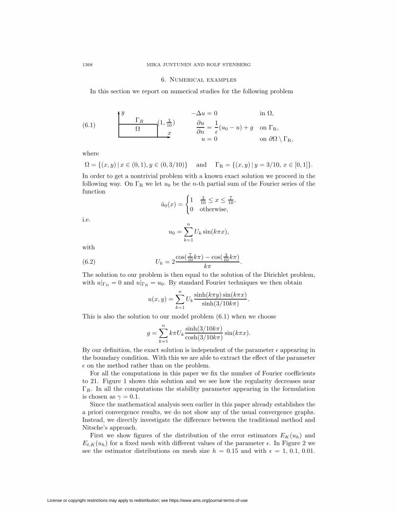
6. Numerical examples
In this section we report on numerical studies for the following problem
(6.1)
x
y
(1, 310 )
ΩΓR
−∆u = 0∂u
∂n=
1ε(u0 − u) + g
u = 0
in Ω,
on ΓR,
on ∂Ω \ ΓR,
where
Ω = (x, y) |x ∈ (0, 1), y ∈ (0, 3/10) and ΓR = (x, y) | y = 3/10, x ∈ [0, 1].In order to get a nontrivial problem with a known exact solution we proceed in thefollowing way. On ΓR we let u0 be the n-th partial sum of the Fourier series of thefunction
u0(x) =
1 3
10 ≤ x ≤ 710 ,
0 otherwise,
i.e.
u0 =n∑
k=1
Uk sin(kπx),
with
(6.2) Uk = 2cos( 7
10kπ) − cos( 310kπ)
kπ.
The solution to our problem is then equal to the solution of the Dirichlet problem,with u|ΓD = 0 and u|ΓR = u0. By standard Fourier techniques we then obtain
u(x, y) =n∑
k=1
Uksinh(kπy) sin(kπx)
sinh(3/10kπ).
This is also the solution to our model problem (6.1) when we choose
g =n∑
k=1
kπUksinh(3/10kπ)cosh(3/10kπ)
sin(kπx).
By our definition, the exact solution is independent of the parameter ε appearing inthe boundary condition. With this we are able to extract the effect of the parameterε on the method rather than on the problem.
For all the computations in this paper we fix the number of Fourier coefficientsto 21. Figure 1 shows this solution and we see how the regularity decreases nearΓR. In all the computations the stability parameter appearing in the formulationis chosen as γ = 0.1.
Since the mathematical analysis seen earlier in this paper already establishes thea priori convergence results, we do not show any of the usual convergence graphs.Instead, we directly investigate the difference between the traditional method andNitsche’s approach.
First we show figures of the distribution of the error estimators EK(uh) andEt,K(uh) for a fixed mesh with different values of the parameter ε. In Figure 2 wesee the estimator distributions on mesh size h = 0.15 and with ε = 1, 0.1, 0.01.
License or copyright restrictions may apply to redistribution; see https://www.ams.org/journal-terms-of-use
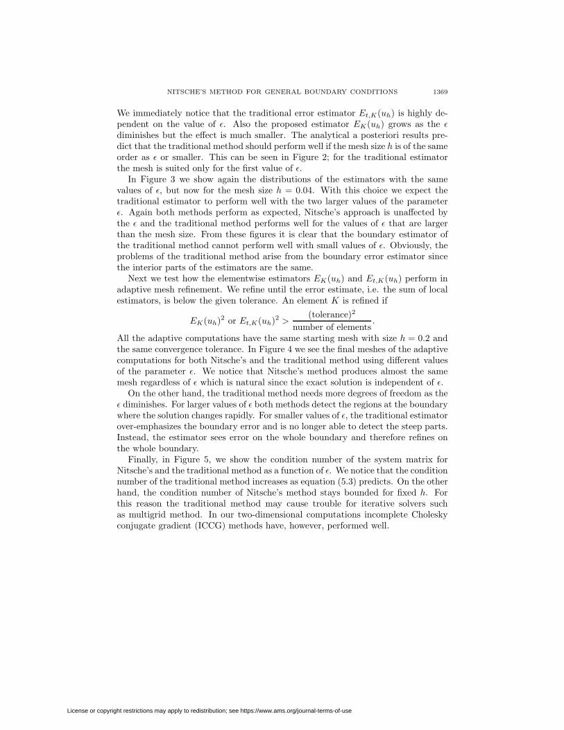
NITSCHE’S METHOD FOR GENERAL BOUNDARY CONDITIONS 1369
We immediately notice that the traditional error estimator Et,K(uh) is highly de-pendent on the value of ε. Also the proposed estimator EK(uh) grows as the εdiminishes but the effect is much smaller. The analytical a posteriori results pre-dict that the traditional method should perform well if the mesh size h is of the sameorder as ε or smaller. This can be seen in Figure 2; for the traditional estimatorthe mesh is suited only for the first value of ε.
In Figure 3 we show again the distributions of the estimators with the samevalues of ε, but now for the mesh size h = 0.04. With this choice we expect thetraditional estimator to perform well with the two larger values of the parameterε. Again both methods perform as expected, Nitsche’s approach is unaffected bythe ε and the traditional method performs well for the values of ε that are largerthan the mesh size. From these figures it is clear that the boundary estimator ofthe traditional method cannot perform well with small values of ε. Obviously, theproblems of the traditional method arise from the boundary error estimator sincethe interior parts of the estimators are the same.
Next we test how the elementwise estimators EK(uh) and Et,K(uh) perform inadaptive mesh refinement. We refine until the error estimate, i.e. the sum of localestimators, is below the given tolerance. An element K is refined if
EK(uh)2 or Et,K(uh)2 >(tolerance)2
number of elements.
All the adaptive computations have the same starting mesh with size h = 0.2 andthe same convergence tolerance. In Figure 4 we see the final meshes of the adaptivecomputations for both Nitsche’s and the traditional method using different valuesof the parameter ε. We notice that Nitsche’s method produces almost the samemesh regardless of ε which is natural since the exact solution is independent of ε.
On the other hand, the traditional method needs more degrees of freedom as theε diminishes. For larger values of ε both methods detect the regions at the boundarywhere the solution changes rapidly. For smaller values of ε, the traditional estimatorover-emphasizes the boundary error and is no longer able to detect the steep parts.Instead, the estimator sees error on the whole boundary and therefore refines onthe whole boundary.
Finally, in Figure 5, we show the condition number of the system matrix forNitsche’s and the traditional method as a function of ε. We notice that the conditionnumber of the traditional method increases as equation (5.3) predicts. On the otherhand, the condition number of Nitsche’s method stays bounded for fixed h. Forthis reason the traditional method may cause trouble for iterative solvers suchas multigrid method. In our two-dimensional computations incomplete Choleskyconjugate gradient (ICCG) methods have, however, performed well.
License or copyright restrictions may apply to redistribution; see https://www.ams.org/journal-terms-of-use

1370 MIKA JUNTUNEN AND ROLF STENBERG
0
0.5
10
0.2
0.4
−0.2
0
0.2
0.4
0.6
0.8
1
1.2
y
The exact solution
x
u
Figure 1. The exact solution to the model problem with 21 termson the boundary data. Recall that the design of the model problemis such that the solution is independent of the boundary conditionparameter ε.
License or copyright restrictions may apply to redistribution; see https://www.ams.org/journal-terms-of-use

NITSCHE’S METHOD FOR GENERAL BOUNDARY CONDITIONS 1371
00.5
1
00.2
0.40
1
2
x
Traditional, ε=1
y 00.5
1
00.2
0.40
1
2
x
Nitsche, ε=1
y
00.5
1
00.2
0.40
10
20
x
Traditional, ε=0.1
y 00.5
1
00.2
0.40
1
2
x
Nitsche, ε=0.1
y
00.5
1
00.2
0.40
500
x
Traditional, ε=0.01
y 00.5
1
00.2
0.40
2
4
x
Nitsche, ε=0.01
y
Figure 2. Distribution of the error estimators with different val-ues of the boundary parameter ε. On the left we have the tradi-tional estimator and on the right the Nitsche estimator. From topto bottom ε has values 1, 0.1 and 0.01. The mesh has size h = 0.15.Notice the scales and how dramatically the traditional estimatordepends on ε.
License or copyright restrictions may apply to redistribution; see https://www.ams.org/journal-terms-of-use

1372 MIKA JUNTUNEN AND ROLF STENBERG
00.5
1
00.2
0.40
0.5
x
Traditional, ε=1
y 00.5
1
00.2
0.40
0.5
x
Nitsche, ε=1
y
00.5
1
00.2
0.40
2
4
x
Traditional, ε=0.1
y 00.5
1
00.2
0.40
0.5
x
Nitsche, ε=0.1
y
00.5
1
00.2
0.40
50
100
x
Traditional, ε=0.01
y 00.5
1
00.2
0.40
0.5
1
x
Nitsche, ε=0.01
y
Figure 3. Distribution of the error estimators with different val-ues of the boundary parameter ε. On the left we have the tradi-tional estimator and on the right the Nitsche estimator. From topto bottom ε has values 1, 0.1 and 0.01. The mesh has size h = 0.04.Notice the scales.
License or copyright restrictions may apply to redistribution; see https://www.ams.org/journal-terms-of-use

NITSCHE’S METHOD FOR GENERAL BOUNDARY CONDITIONS 1373
0 0.5 10
0.2
0.4
Nitsche’s method, ε=0.1degrees of freedom: 174
0 0.5 10
0.2
0.4
the traditional method, ε=0.1
degrees of freedom: 174
0 0.5 10
0.2
0.4
Nitsche’s method, ε=0.01
degrees of freedom: 177
0 0.5 10
0.2
0.4
the traditional method, ε=0.01
degrees of freedom: 187
0 0.5 10
0.2
0.4
Nitsche’s method, ε=0.001
degrees of freedom: 177
0 0.5 10
0.2
0.4
the traditional method, ε=0.001
degrees of freedom: 432
0 0.5 10
0.2
0.4
Nitsche’s method, ε=0.0001
degrees of freedom: 177
0 0.5 10
0.2
0.4
the traditional method, ε=0.0001
degrees of freedom: 846
Figure 4. The final meshes of the adaptive refinement that fulfillthe given tolerance. On the left meshes of Nitsche’s method andon the right meshes of the traditional method. Notice that thetraditional method is unable to detect the difficult parts of thesolution with small ε. Recall that the exact solution does notdepend on ε.
License or copyright restrictions may apply to redistribution; see https://www.ams.org/journal-terms-of-use

1374 MIKA JUNTUNEN AND ROLF STENBERG
10−8
10−6
10−4
10−2
100
102
104
102
104
106
108
parameter ε
cond
ition
num
ber
Condition number of the system matrix
Nitsche’s methodtraditional method
Figure 5. The condition number of the system matrix as a func-tion of ε for fixed h and for both Nitsche’s and the traditionalmethod. Notice the growth of condition number in the traditionalmethod; see equation (5.3).
References
1. Douglas N. Arnold, Franco Brezzi, Bernardo Cockburn, and L. Donatella Marini, Unifiedanalysis of discontinuous Galerkin methods for elliptic problems, SIAM J. Numer. Anal. 39(2001/02), no. 5, 1749–1779 (electronic). MR1885715 (2002k:65183)
2. Ivo Babuska, Uday Banerjee, and John E. Osborn, Survey of meshless and generalized finiteelement methods: a unified approach, Acta Numer. 12 (2003), 1–125. MR2249154
3. Roland Becker, Peter Hansbo, and Rolf Stenberg, A finite element methods for domain de-composition with non-matching grids, Mathematical Modelling and Numerical Analysis 37(2003), no. 2, 209–225. MR1991197 (2004e:65129)
4. D. Braess and R. Verfurth, A posteriori error estimator for the Raviart-Thomas element,SIAM J. Numer. Anal 33 (1996), 2431–2444. MR1427472 (97m:65201)
5. Philippe G. Ciarlet, The finite element methods for elliptic problems, second ed., North-Holland, 1987. MR0520174 (58:25001)
6. J.A. Nitsche, Uber ein Variationsprinzip zur Losung von Dirichlet-Problemen bei Verwen-
dung von Teilraumen, die keinen Randbedingungen unterworfen sind, Abhandlungen ausdem Mathematischen Seminar der Universitat Hamburg 36 (1970/71), 9–15. MR0341903(49:6649)
7. Rolf Stenberg, Mortaring by a method of J.A. Nitsche, Computational Mechanics; New Trendsand Applications, S. Idelsohn, E. Onate and E. Dvorkin (Eds.) (CIMNE, Barcelona, Spain,1998). MR1839048
8. Rudiger Verfurth, A review of a posteriori error estimation and adaptive mesh refinementtechniques, Wiley, 1996.
Institute of Mathematics, Helsinki University of Technology, P. O. Box 1100, 02015
TKK, Finland
E-mail address: [email protected]
Institute of Mathematics, Helsinki University of Technology, P. O. Box 1100, 02015
TKK, Finland
License or copyright restrictions may apply to redistribution; see https://www.ams.org/journal-terms-of-use