introduction to algebraic number theory - william a. stein · 10 chapter 1. introduction 1.2 what...

Introduction to

Algebraic Number Theory

William Stein

May 5, 2005

Contents

1 Introduction 9

1.1 Mathematical background I assume you have . . . . . . . . . . . . . 9

1.2 What is algebraic number theory? . . . . . . . . . . . . . . . . . . . 10

1.2.1 Topics in this book . . . . . . . . . . . . . . . . . . . . . . . . 10

1.3 Some applications of algebraic number theory . . . . . . . . . . . . . 11

I Algebraic Number Fields 13

2 Basic Commutative Algebra 15

2.1 Finitely Generated Abelian Groups . . . . . . . . . . . . . . . . . . . 15

2.2 Noetherian Rings and Modules . . . . . . . . . . . . . . . . . . . . . 18

2.2.1 The Ring Z is noetherian . . . . . . . . . . . . . . . . . . . . 22

2.3 Rings of Algebraic Integers . . . . . . . . . . . . . . . . . . . . . . . 22

2.4 Norms and Traces . . . . . . . . . . . . . . . . . . . . . . . . . . . . 25

3 Unique Factorization of Ideals 29

3.1 Dedekind Domains . . . . . . . . . . . . . . . . . . . . . . . . . . . . 29

4 Computing 37

4.1 Algorithms for Algebraic Number Theory . . . . . . . . . . . . . . . 37

4.2 Magma . . . . . . . . . . . . . . . . . . . . . . . . . . . . . . . . . . 37

4.2.1 Smith Normal Form . . . . . . . . . . . . . . . . . . . . . . . 38

4.2.2 Number Fields . . . . . . . . . . . . . . . . . . . . . . . . . . 40

4.2.3 Relative Extensions . . . . . . . . . . . . . . . . . . . . . . . 40

4.2.4 Rings of integers . . . . . . . . . . . . . . . . . . . . . . . . . 41

4.2.5 Ideals . . . . . . . . . . . . . . . . . . . . . . . . . . . . . . . 43

4.3 Using PARI . . . . . . . . . . . . . . . . . . . . . . . . . . . . . . . . 45

4.3.1 Smith Normal Form . . . . . . . . . . . . . . . . . . . . . . . 46

4.3.2 Number Fields . . . . . . . . . . . . . . . . . . . . . . . . . . 47

4.3.3 Rings of integers . . . . . . . . . . . . . . . . . . . . . . . . . 48

4.3.4 Ideals . . . . . . . . . . . . . . . . . . . . . . . . . . . . . . . 49

3

4 CONTENTS

5 Factoring Primes 51

5.1 The Problem . . . . . . . . . . . . . . . . . . . . . . . . . . . . . . . 51

5.1.1 Geomtric Intuition . . . . . . . . . . . . . . . . . . . . . . . . 52

5.1.2 Examples . . . . . . . . . . . . . . . . . . . . . . . . . . . . . 52

5.2 A Method for Factoring Primes that Often Works . . . . . . . . . . 54

5.3 A General Method . . . . . . . . . . . . . . . . . . . . . . . . . . . . 57

5.3.1 Essential Discriminant Divisors . . . . . . . . . . . . . . . . . 58

5.3.2 Remarks on Ideal Factorization in General . . . . . . . . . . . 58

5.3.3 Finding a p-Maximal Order . . . . . . . . . . . . . . . . . . . 59

5.3.4 General Factorization Algorithm . . . . . . . . . . . . . . . . 60

5.4 Appendix: The Calculations in PARI . . . . . . . . . . . . . . . . . . 61

6 The Chinese Remainder Theorem 63

6.1 The Chinese Remainder Theorem . . . . . . . . . . . . . . . . . . . . 63

6.1.1 CRT in the Integers . . . . . . . . . . . . . . . . . . . . . . . 63

6.1.2 CRT in an Arbitrary Ring . . . . . . . . . . . . . . . . . . . . 64

6.2 Computing Using the CRT . . . . . . . . . . . . . . . . . . . . . . . 65

6.2.1 Magma . . . . . . . . . . . . . . . . . . . . . . . . . . . . . . 66

6.2.2 PARI . . . . . . . . . . . . . . . . . . . . . . . . . . . . . . . 66

6.3 Structural Applications of the CRT . . . . . . . . . . . . . . . . . . . 67

7 Discrimants and Norms 71

7.1 Field Embeddings . . . . . . . . . . . . . . . . . . . . . . . . . . . . 71

7.2 Discriminants . . . . . . . . . . . . . . . . . . . . . . . . . . . . . . . 73

7.3 Norms of Ideals . . . . . . . . . . . . . . . . . . . . . . . . . . . . . . 75

8 Finiteness of the Class Group 77

8.1 The Class Group . . . . . . . . . . . . . . . . . . . . . . . . . . . . . 77

8.2 Class Number 1 . . . . . . . . . . . . . . . . . . . . . . . . . . . . . . 82

8.3 More About Computing Class Groups . . . . . . . . . . . . . . . . . 84

9 Dirichlet’s Unit Theorem 87

9.1 The Group of Units . . . . . . . . . . . . . . . . . . . . . . . . . . . 87

9.2 Examples with MAGMA . . . . . . . . . . . . . . . . . . . . . . . . . 92

9.2.1 Pell’s Equation . . . . . . . . . . . . . . . . . . . . . . . . . . 92

9.2.2 Examples with Various Signatures . . . . . . . . . . . . . . . 94

10 Decomposition and Inertia Groups 99

10.1 Galois Extensions . . . . . . . . . . . . . . . . . . . . . . . . . . . . . 99

10.2 Decomposition of Primes: efg = n . . . . . . . . . . . . . . . . . . . 101

10.2.1 Quadratic Extensions . . . . . . . . . . . . . . . . . . . . . . 102

10.2.2 The Cube Root of Two . . . . . . . . . . . . . . . . . . . . . 103

10.3 The Decomposition Group . . . . . . . . . . . . . . . . . . . . . . . . 103

10.3.1 Galois groups of finite fields . . . . . . . . . . . . . . . . . . . 105

CONTENTS 5

10.3.2 The Exact Sequence . . . . . . . . . . . . . . . . . . . . . . . 10610.4 Frobenius Elements . . . . . . . . . . . . . . . . . . . . . . . . . . . . 10710.5 Galois Representations, L-series and a Conjecture of Artin . . . . . . 107

11 Elliptic Curves, Galois Representations, and L-functions 11111.1 Groups Attached to Elliptic Curves . . . . . . . . . . . . . . . . . . . 111

11.1.1 Abelian Groups Attached to Elliptic Curves . . . . . . . . . . 11211.1.2 A Formula for Adding Points . . . . . . . . . . . . . . . . . . 11411.1.3 Other Groups . . . . . . . . . . . . . . . . . . . . . . . . . . . 114

11.2 Galois Representations Attached to Elliptic Curves . . . . . . . . . . 11511.2.1 Modularity of Elliptic Curves over Q . . . . . . . . . . . . . . 116

12 Galois Cohomology 11912.1 Group Cohomology . . . . . . . . . . . . . . . . . . . . . . . . . . . . 119

12.1.1 Group Rings . . . . . . . . . . . . . . . . . . . . . . . . . . . 11912.2 Modules and Group Cohomology . . . . . . . . . . . . . . . . . . . . 119

12.2.1 Example Application of the Theorem . . . . . . . . . . . . . . 12112.3 Inflation and Restriction . . . . . . . . . . . . . . . . . . . . . . . . . 12212.4 Galois Cohomology . . . . . . . . . . . . . . . . . . . . . . . . . . . . 123

13 The Weak Mordell-Weil Theorem 12513.1 Kummer Theory of Number Fields . . . . . . . . . . . . . . . . . . . 12513.2 Proof of the Weak Mordell-Weil Theorem . . . . . . . . . . . . . . . 127

14 Exercises 131

6 CONTENTS

Preface

This book is based on notes I created for a one-semester undergraduate courseon Algebraic Number Theory, which I taught at Harvard during Spring 2004 andSpring 2005. The textbook for the first course was chapter 1 of Swinnerton-Dyer’sbook [SD01]. The first draft of this book followed [SD01] closely, but the currentversion but adding substantial text and examples to make the mathematics accessi-ble to advanced undergraduates. For example, chapter 1 of [SD01] is only 30 pages,whereas this book is 140 pages.

—————————

- Copyright: William Stein, 2005.

License: This book my be freely redistributed, printed and copied, even withoutwritten permission from me. You may even extend or change this book, but thispreface page must remain in any derived work, and any derived work must alsoremain free, including the LATEX source files.

Please send any typos or corrections to [email protected].

7

8 CONTENTS

Acknowledgement: This book closely builds on Swinnerton-Dyer’s book [SD01]and Cassels’s article [Cas67]. Many of the students of Math 129 at Harvard dur-ing Spring 2004 and 2005 made helpful comments: Jennifer Balakrishnan, PeterBehrooz, Jonathan Bloom, David Escott Jayce Getz, Michael Hamburg, Deniz Ku-ral, Danielle li, Andrew Ostergaard, Gregory Price, Grant Schoenebeck, JenniferSinnott, Stephen Walker, Daniel Weissman, and Inna Zakharevich in 2004; MauroBraunstein, Steven Byrnes, William Fithian, Frank Kelly, Alison Miller, Nizamed-din Ordulu, Corina Patrascu, Anatoly Preygel, Emily Riehl, Gary Sivek, StevenSivek, Kaloyan Slavov, Gregory Valiant, and Yan Zhang in 2005. Also the courseassistants Matt Bainbridge and Andrei Jorza made many helpful comments.

This material is based upon work supported by the National Science Foundationunder Grant No. 0400386.

Chapter 1

Introduction

1.1 Mathematical background I assume you have

In addition to general mathematical maturity, this book assumes you have thefollowing background:

• Basics of finite group theory

• Commutative rings, ideals, quotient rings

• Some elementary number theory

• Basic Galois theory of fields

• Point set topology

• Basic of topological rings, groups, and measure theory

For example, if you have never worked with finite groups before, you should readanother book first. If you haven’t seen much elementary ring theory, there is stillhope, but you will have to do some additional reading and exercises. I will brieflyreview the basics of the Galois theory of number fields.

Some of the homework problems involve using a computer, but I’ll give youexamples which you can build on. I will not assume that you have a programmingbackground or know much about algorithms. If you don’t have PARI [ABC+] orMagma [BCP97], and don’t want to install either one on your computer, you mightwant to try the following online interface to PARI and Magma:

http://modular.fas.harvard.edu/calc/

9

10 CHAPTER 1. INTRODUCTION

1.2 What is algebraic number theory?

A number field K is a finite algebraic extension of the rational numbers Q. Everysuch extension can be represented as all polynomials in an algebraic number α:

K = Q(α) =

{m∑

n=0

anαn : an ∈ Q

}.

Here α is a root of a polynomial with coefficients in Q.

Algebraic number theory involves using techniques from (mostly commutative)algebra and finite group theory to gain a deeper understanding of number fields.The main objects that we study in algebraic number theory are number fields,rings of integers of number fields, unit groups, ideal class groups,norms, traces,discriminants, prime ideals, Hilbert and other class fields and associated reciprocitylaws, zeta and L-functions, and algorithms for computing each of the above.

1.2.1 Topics in this book

These are some of the main topics that are discussed in this book:

• Rings of integers of number fields

• Unique factorization of ideals in Dedekind domains

• Structure of the group of units of the ring of integers

• Finiteness of the group of equivalence classes of ideals of the ring of integers(the “class group”)

• Decomposition and inertia groups, Frobenius elements

• Ramification

• Discriminant and different

• Quadratic and biquadratic fields

• Cyclotomic fields (and applications)

• How to use a computer to compute with many of the above objects (bothalgorithms and actual use of PARI and Magma).

• Valuations on fields

• Completions (p-adic fields)

• Adeles and Ideles

1.3. SOME APPLICATIONS OF ALGEBRAIC NUMBER THEORY 11

Note that we will not do anything nontrivial with zeta functions or L-functions.This is to keep the prerequisites to algebra, and so we will have more time todiscuss algorithmic questions. Depending on time and your inclination, I may alsotalk about integer factorization, primality testing, or complex multiplication ellipticcurves (which are closely related to quadratic imaginary fields).

1.3 Some applications of algebraic number theory

The following examples are meant to convince you that learning algebraic numbertheory now will be an excellent investment of your time. If an example below seemsvague to you, it is safe to ignore it.

1. Integer factorization using the number field sieve. The number field sieve isthe asymptotically fastest known algorithm for factoring general large integers(that don’t have too special of a form). Recently, in December 2003, thenumber field sieve was used to factor the RSA-576 $10000 challenge:

1881988129206079638386972394616504398071635633794173827007 . . .. . . 6335642298885971523466548531906060650474304531738801130339 . . .. . . 6716199692321205734031879550656996221305168759307650257059= 39807508642406493739712550055038649119906436234252670840 . . .

. . . 6385189575946388957261768583317×47277214610743530253622307197304822463291469530209711 . . .

. . . 6459852171130520711256363590397527

(The . . . indicates that the newline should be removed, not that there aremissing digits.) For more information on the NFS, see the paper by Lenstraet al. on the Math 129 web page.

2. Primality test: Agrawal and his students Saxena and Kayal from India re-cently (2002) found the first ever deterministic polynomial-time (in the num-ber of digits) primality test. There methods involve arithmetic in quotients of(Z/nZ)[x], which are best understood in the context of algebraic number the-ory. For example, Lenstra, Bernstein, and others have done that and improvedthe algorithm significantly.

3. Deeper point of view on questions in number theory:

(a) Pell’s Equation (x2−dy2 = 1) =⇒ Units in real quadratic fields =⇒ Unitgroups in number fields

(b) Diophantine Equations =⇒ For which n does xn + yn = zn have a non-trivial solution?

(c) Integer Factorization =⇒ Factorization of ideals

(d) Riemann Hypothesis =⇒ Generalized Riemann Hypothesis

12 CHAPTER 1. INTRODUCTION

(e) Deeper proof of Gauss’s quadratic reciprocity law in terms of arithmeticof cyclotomic fields Q(e2πi/n), which leads to class field theory.

4. Wiles’s proof of Fermat’s Last Theorem, i.e., xn+yn = zn has no nontrivialinteger solutions, uses methods from algebraic number theory extensively (inaddition to many other deep techniques). Attempts to prove Fermat’s LastTheorem long ago were hugely influential in the development of algebraicnumber theory (by Dedekind, Kummer, Kronecker, et al.).

5. Arithmetic geometry: This is a huge field that studies solutions to polyno-mial equations that lie in arithmetically interesting rings, such as the integersor number fields. A famous major triumph of arithmetic geometry is Faltings’sproof of Mordell’s Conjecture.

Theorem 1.3.1 (Faltings). Let X be a plane algebraic curve over a numberfield K. Assume that the manifold X(C) of complex solutions to X has genusat least 2 (i.e., X(C) is topologically a donut with two holes). Then the setX(K) of points on X with coordinates in K is finite.

For example, Theorem 1.3.1 implies that for any n ≥ 4 and any numberfield K, there are only finitely many solutions in K to xn + yn = 1.

A major open problem in arithmetic geometry is the Birch and Swinnerton-Dyer conjecture. Suppose X is an algebraic curve such that the set of com-plex points X(C) is a topological torus. Then the conjecture of Birch andSwinnerton-Dyer gives a criterion for whether or not X(K) is infinite in termsof analytic properties of the L-function L(X, s).

Part I

Algebraic Number Fields

13

Chapter 2

Basic Commutative Algebra

The commutative algebra in this chapter will provide a solid algebraic foundation forunderstanding the more refined number-theoretic structures associated to numberfields.

First we prove the structure theorem for finitely generated abelian groups. Thenwe establish the standard properties of Noetherian rings and modules, including aproof of the Hilbert basis theorem. We also observe that finitely generated abeliangroups are Noetherian Z-modules. After establishing properties of Noetherian rings,we consider rings of algebraic integers and discuss some of their properties.

2.1 Finitely Generated Abelian Groups

We will now prove the structure theorem for finitely generated abelian groups, sinceit will be crucial for much of what we will do later.

Let Z = {0,±1,±2, . . .} denote the ring of integers, and for each positive inte-ger n let Z/nZ denote the ring of integers modulo n, which is a cyclic abelian groupof order n under addition.

Definition 2.1.1 (Finitely Generated). A group G is finitely generated if thereexists g1, . . . , gn ∈ G such that every element of G can be obtained from the gi.

For example, the group Z is finitely generated, since it is generated by 1.

Theorem 2.1.2 (Structure Theorem for Abelian Groups). Let G be a finitelygenerated abelian group. Then there is an isomorphism

G ∼= (Z/n1Z) ⊕ (Z/n2Z) ⊕ · · · ⊕ (Z/nsZ) ⊕ Zr,

where n1 > 1 and n1 | n2 | · · · | ns. Furthermore, the ni and r are uniquelydetermined by G.

We will prove the theorem as follows. We first remark that any subgroup of afinitely generated free abelian group is finitely generated. Then we see that finitely

15

16 CHAPTER 2. BASIC COMMUTATIVE ALGEBRA

generated abelian groups can be presented as quotients of finite rank free abeliangroups, and such a presentation can be reinterpreted in terms of matrices over theintegers. Next we describe how to use row and column operations over the integersto show that every matrix over the integers is equivalent to one in a canonicaldiagonal form, called the Smith normal form. We obtain a proof of the theorem byreinterpreting Smith normal form in terms of groups.

Proposition 2.1.3. Suppose G is a free abelian group of finite rank n, and H is asubgroup of G. Then H is a free abelian group generated by at most n elements.

The key reason that this is true is that G is a finitely generated module over theprincipal ideal domain Z. We will give a complete proof of a beautiful generalizationof this result in the context of Noetherian rings next time, but will not prove thisproposition here.

Corollary 2.1.4. Suppose G is a finitely generated abelian group. Then there arefinitely generated free abelian groups F1 and F2 such that G ∼= F1/F2.

Proof. Let x1, . . . , xm be generators for G. Let F1 = Zm and let ϕ : F1 → G bethe map that sends the ith generator (0, 0, . . . , 1, . . . , 0) of Zm to xi. Then ϕ is asurjective homomorphism, and by Proposition 2.1.3 the kernel F2 of ϕ is a finitelygenerated free abelian group. This proves the corollary.

Suppose G is a nonzero finitely generated abelian group. By the corollary, thereare free abelian groups F1 and F2 such that G ∼= F1/F2. Choosing a basis for F1, weobtain an isomorphism F1

∼= Zn, for some positive integer n. By Proposition 2.1.3,F2

∼= Zm, for some integer m with 0 ≤ m ≤ n, and the inclusion map F2 ↪→ F1

induces a map Zm → Zn. This homomorphism is left multiplication by the n × mmatrix A whose columns are the images of the generators of F2 in Zn. The cokernelof this homomorphism is the quotient of Zn by the image of A, and the cokernelis isomorphic to G. By augmenting A with zero columns on the right we obtain asquare n × n matrix A with the same cokernel. The following proposition impliesthat we may choose bases such that the matrix A is diagonal, and then the structureof the cokernel of A will be easy to understand.

Proposition 2.1.5 (Smith normal form). Suppose A is an n×n integer matrix.Then there exist invertible integer matrices P and Q such that A′ = PAQ is adiagonal matrix with entries n1, n2, . . . , ns, 0, . . . , 0, where n1 > 1 and n1 | n2 | . . . |ns. Here P and Q are invertible as integer matrices, so det(P ) and det(Q) are ±1.The matrix A′ is called the Smith normal form of A.

We will see in the proof of Theorem 2.1.2 that A′ is uniquely determined by A.An example of a matrix in Smith normal form is

A =

2 0 00 6 00 0 0

.

2.1. FINITELY GENERATED ABELIAN GROUPS 17

Proof. The matrix P will be a product of matrices that define elementary rowoperations and Q will be a product corresponding to elementary column operations.The elementary row and column operations are as follows:

1. [Add multiple] Add an integer multiple of one row to another (or a multipleof one column to another).

2. [Swap] Interchange two rows or two columns.

3. [Rescale] Multiply a row by −1.

Each of these operations is given by left or right multiplying by an invertible ma-trix E with integer entries, where E is the result of applying the given operationto the identity matrix, and E is invertible because each operation can be reversedusing another row or column operation over the integers.

To see that the proposition must be true, assume A 6= 0 and perform the fol-lowing steps (compare [Art91, pg. 459]):

1. By permuting rows and columns, move a nonzero entry of A with smallestabsolute value to the upper left corner of A. Now attempt to make all otherentries in the first row and column 0 by adding multiples of row or column 1to other rows (see step 2 below). If an operation produces a nonzero entry inthe matrix with absolute value smaller than |a11|, start the process over bypermuting rows and columns to move that entry to the upper left corner ofA. Since the integers |a11| are a decreasing sequence of positive integers, wewill not have to move an entry to the upper left corner infinitely often.

2. Suppose ai1 is a nonzero entry in the first column, with i > 1. Using thedivision algorithm, write ai1 = a11q + r, with 0 ≤ r < a11. Now add −q timesthe first row to the ith row. If r > 0, then go to step 1 (so that an entry withabsolute value at most r is the upper left corner). Since we will only performstep 1 finitely many times, we may assume r = 0. Repeating this procedurewe set all entries in the first column (except a11) to 0. A similar process usingcolumn operations sets each entry in the first row (except a11) to 0.

3. We may now assume that a11 is the only nonzero entry in the first row andcolumn. If some entry aij of A is not divisible by a11, add the column of Acontaining aij to the first column, thus producing an entry in the first columnthat is nonzero. When we perform step 2, the remainder r will be greaterthan 0. Permuting rows and columns results in a smaller |a11|. Since |a11| canonly shrink finitely many times, eventually we will get to a point where everyaij is divisible by a11. If a11 is negative, multiple the first row by −1.

After performing the above operations, the first row and column of A are zero exceptfor a11 which is positive and divides all other entries of A. We repeat the abovesteps for the matrix B obtained from A by deleting the first row and column. Theupper left entry of the resulting matrix will be divisible by a11, since every entry ofB is. Repeating the argument inductively proves the proposition.


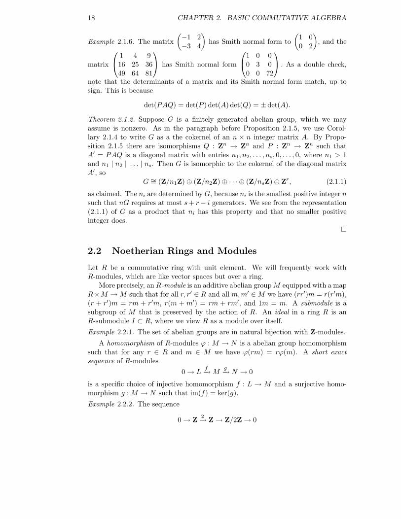
Example 2.1.6. The matrix

(−1 2−3 4

)has Smith normal form to

(1 00 2

), and the

matrix

1 4 916 25 3649 64 81

has Smith normal form

1 0 00 3 00 0 72

. As a double check,

note that the determinants of a matrix and its Smith normal form match, up tosign. This is because

det(PAQ) = det(P ) det(A) det(Q) = ±det(A).

Theorem 2.1.2. Suppose G is a finitely generated abelian group, which we mayassume is nonzero. As in the paragraph before Proposition 2.1.5, we use Corol-lary 2.1.4 to write G as a the cokernel of an n × n integer matrix A. By Propo-sition 2.1.5 there are isomorphisms Q : Zn → Zn and P : Zn → Zn such thatA′ = PAQ is a diagonal matrix with entries n1, n2, . . . , ns, 0, . . . , 0, where n1 > 1and n1 | n2 | . . . | ns. Then G is isomorphic to the cokernel of the diagonal matrixA′, so

G ∼= (Z/n1Z) ⊕ (Z/n2Z) ⊕ · · · ⊕ (Z/nsZ) ⊕ Zr, (2.1.1)

as claimed. The ni are determined by G, because ni is the smallest positive integer nsuch that nG requires at most s + r − i generators. We see from the representation(2.1.1) of G as a product that ni has this property and that no smaller positiveinteger does.

2.2 Noetherian Rings and Modules

Let R be a commutative ring with unit element. We will frequently work withR-modules, which are like vector spaces but over a ring.

More precisely, an R-module is an additive abelian group M equipped with a mapR×M → M such that for all r, r′ ∈ R and all m, m′ ∈ M we have (rr′)m = r(r′m),(r + r′)m = rm + r′m, r(m + m′) = rm + rm′, and 1m = m. A submodule is asubgroup of M that is preserved by the action of R. An ideal in a ring R is anR-submodule I ⊂ R, where we view R as a module over itself.

Example 2.2.1. The set of abelian groups are in natural bijection with Z-modules.

A homomorphism of R-modules ϕ : M → N is a abelian group homomorphismsuch that for any r ∈ R and m ∈ M we have ϕ(rm) = rϕ(m). A short exactsequence of R-modules

0 → Lf−→ M

g−→ N → 0

is a specific choice of injective homomorphism f : L → M and a surjective homo-morphism g : M → N such that im(f) = ker(g).

Example 2.2.2. The sequence

0 → Z2−→ Z → Z/2Z → 0

2.2. NOETHERIAN RINGS AND MODULES 19

is an exact sequence, where the first map sends 1 to 2, and the second is the naturalquotient map.

Definition 2.2.3 (Noetherian). An R-module M is noetherian if every submod-ule of M is finitely generated. A ring R is noetherian if R is noetherian as a moduleover itself, i.e., if every ideal of R is finitely generated.

Notice that any submodule M ′ of a noetherian module M is also noetherian.Indeed, if every submodule of M is finitely generated then so is every submodule ofM ′, since submodules of M ′ are also submodules of M .

Definition 2.2.4 (Ascending chain condition). An R-module M satisfies theascending chain condition if every sequences M1 ⊂ M2 ⊂ M3 ⊂ · · · of submodulesof M eventually stabilizes, i.e., there is some n such that Mn = Mn+1 = Mn+2 = · · · .

We will use the notion of maximal element below. If X is a set of subsets ofa set S, ordered by inclusion, then a maximal element A ∈ X is a set so that nosuperset of A is contained in X . Note that it is not necessary that A contain everyother element of X , and that X could contain many maximal elements.

Proposition 2.2.5. If M is an R-module, then the following are equivalent:

1. M is noetherian,

2. M satisfies the ascending chain condition, and

3. Every nonempty set of submodules of M contains at least one maximal ele-ment.

Proof. 1 =⇒ 2: Suppose M1 ⊂ M2 ⊂ · · · is a sequence of submodules of M .Then M∞ = ∪∞

n=1Mn is a submodule of M . Since M is noetherian and M∞ isa submodule of M , there is a finite set a1, . . . , am of generators for M∞. Each ai

must be contained in some Mj , so there is an n such that a1, . . . , am ∈ Mn. Butthen Mk = Mn for all k ≥ n, which proves that the chain of Mi stabilizes, so theascending chain condition holds for M .2 =⇒ 3: Suppose 3 were false, so there exists a nonempty set S of submodulesof M that does not contain a maximal element. We will use S to construct aninfinite ascending chain of submodules of M that does not stabilize. Note that S isinfinite, otherwise it would contain a maximal element. Let M1 be any element of S.Then there is an M2 in S that contains M1, otherwise S would contain the maximalelement M1. Continuing inductively in this way we find an M3 in S that properlycontains M2, etc., and we produce an infinite ascending chain of submodules of M ,which contradicts the ascending chain condition.3 =⇒ 1: Suppose 1 is false, so there is a submodule M ′ of M that is not finitelygenerated. We will show that the set S of all finitely generated submodules ofM ′ does not have a maximal element, which will be a contradiction. Suppose Sdoes have a maximal element L. Since L is finitely generated and L ⊂ M ′, and


M ′ is not finitely generated, there is an a ∈ M ′ such that a 6∈ L. Then L′ =L + Ra is an element of S that strictly contains the presumed maximal element L,a contradiction.

Lemma 2.2.6. If

0 → Lf−→ M

g−→ N → 0

is a short exact sequence of R-modules, then M is noetherian if and only if both Land N are noetherian.

Proof. First suppose that M is noetherian. Then L is a submodule of M , so L isnoetherian. If N ′ is a submodule of N , then the inverse image of N ′ in M is asubmodule of M , so it is finitely generated, hence its image N ′ is finitely generated.Thus N is noetherian as well.

Next assume nothing about M , but suppose that both L and N are noetherian.If M ′ is a submodule of M , then M0 = ϕ(L)∩M ′ is isomorphic to a submodule of thenoetherian module L, so M0 is generated by finitely many elements a1, . . . , an. Thequotient M ′/M0 is isomorphic (via g) to a submodule of the noetherian module N ,so M ′/M0 is generated by finitely many elements b1, . . . , bm. For each i ≤ m, let ci

be a lift of bi to M ′, modulo M0. Then the elements a1, . . . , an, c1, . . . , cm generateM ′, for if x ∈ M ′, then there is some element y ∈ M0 such that x− y is an R-linearcombination of the ci, and y is an R-linear combination of the ai.

Proposition 2.2.7. Suppose R is a noetherian ring. Then an R-module M isnoetherian if and only if it is finitely generated.

Proof. If M is noetherian then every submodule of M is finitely generated so Mis finitely generated. Conversely, suppose M is finitely generated, say by elementsa1, . . . , an. Then there is a surjective homomorphism from Rn = R ⊕ · · · ⊕ R to Mthat sends (0, . . . , 0, 1, 0, . . . , 0) (1 in ith factor) to ai. Using Lemma 2.2.6 andexact sequences of R-modules such as 0 → R → R⊕R → R → 0, we see inductivelythat Rn is noetherian. Again by Lemma 2.2.6, homomorphic images of noetherianmodules are noetherian, so M is noetherian.

Lemma 2.2.8. Suppose ϕ : R → S is a surjective homomorphism of rings and Ris noetherian. Then S is noetherian.

Proof. The kernel of ϕ is an ideal I in R, and we have an exact sequence

0 → I → R → S → 0

with R noetherian. This is an exact sequence of R-modules, where S has the R-module structure induced from ϕ (if r ∈ R and s ∈ S, then rs = ϕ(r)s). ByLemma 2.2.6, it follows that S is a noetherian R-modules. Suppose J is an idealof S. Since J is an R-submodule of S, if we view J as an R-module, then J isfinitely generated. Since R acts on J through S, the R-generators of J are alsoS-generators of J , so J is finitely generated as an ideal. Thus S is noetherian.

2.2. NOETHERIAN RINGS AND MODULES 21

Theorem 2.2.9 (Hilbert Basis Theorem). If R is a noetherian ring and S isfinitely generated as a ring over R, then S is noetherian. In particular, for any nthe polynomial ring R[x1, . . . , xn] and any of its quotients are noetherian.

Proof. Assume first that we have already shown that for any n the polynomial ringR[x1, . . . , xn] is noetherian. Suppose S is finitely generated as a ring over R, sothere are generators s1, . . . , sn for S. Then the map xi 7→ si extends uniquely to asurjective homomorphism π : R[x1, . . . , xn] → S, and Lemma 2.2.8 implies that Sis noetherian.

The rings R[x1, . . . , xn] and (R[x1, . . . , xn−1])[xn] are isomorphic, so it sufficesto prove that if R is noetherian then R[x] is also noetherian. (Our proof follows[Art91, §12.5].) Thus suppose I is an ideal of R[x] and that R is noetherian. Wewill show that I is finitely generated.

Let A be the set of leading coefficients of polynomials in I. (The leading coeffi-cient of a polynomial is the coefficient of highest degree, or 0 if the polynomial is 0;thus 3x7 + 5x2 − 4 has leading coefficient 3.) We will first show that A is an idealof R. Suppose a, b ∈ A are nonzero with a + b 6= 0. Then there are polynomials fand g in I with leading coefficients a and b. If deg(f) ≤ deg(g), then a + b is theleading coefficient of xdeg(g)−deg(f)f + g, so a + b ∈ A. Suppose r ∈ R and a ∈ Awith ra 6= 0. Then ra is the leading coefficient of rf , so ra ∈ A. Thus A is an idealin R.

Since R is noetherian and A is an ideal, there exist nonzero a1, . . . , an thatgenerate A as an ideal. Since A is the set of leading coefficients of elements of I,and the aj are in A, we can choose for each j ≤ n an element fj ∈ I with leadingcoefficient aj . By multipying the fj by some power of x, we may assume that thefj all have the same degree d ≥ 1.

Let S<d be the set of elements of I that have degree strictly less than d. Thisset is closed under addition and under multiplication by elements of R, so S<d is amodule over R. The module S<d is the submodule of the R-module of polynomialsof degree less than n, which is noetherian because it is generated by 1, x, . . . , xn−1.Thus S<d is finitely generated, and we may choose generators h1, . . . , hm for S<d.

We finish by proving using induction on the degree that every g ∈ I is an R[x]-linear combination of f1, . . . , fn, h1, . . . hm. If g ∈ I has degree 0, then g ∈ S<d, sinced ≥ 1, so g is a linear combination of h1, . . . , hm. Next suppose g ∈ I has degree e,and that we have proven the statement for all elements of I of degree < e. If e ≤ d,then g ∈ S<d, so g is in the R[x]-ideal generated by h1, . . . , hm. Next suppose thate ≥ d. Then the leading coefficient b of g lies in the ideal A of leading coefficientsof elements of I, so there exist ri ∈ R such that b = r1a1 + · · ·+ rnan. Since fi hasleading coefficient ai, the difference g − xe−drifi has degree less than the degree eof g. By induction g−xe−drifi is an R[x] linear combination of f1, . . . , fn, h1, . . . hm,so g is also an R[x] linear combination of f1, . . . , fn, h1, . . . hm. Since each fi andhj lies in I, it follows that I is generated by f1, . . . , fn, h1, . . . hm, so I is finitelygenerated, as required.

Properties of noetherian rings and modules will be crucial in the rest of this


course. We have proved above that noetherian rings have many desirable properties.

2.2.1 The Ring Z is noetherian

The ring Z of integers is noetherian because every ideal of Z is generated by oneelement.

Proposition 2.2.10. Every ideal of the ring Z of integers is principal.

Proof. Suppose I is a nonzero ideal in Z. Let d the least positive element of I.Suppose that a ∈ I is any nonzero element of I. Using the division algorithm, writea = dq + r, where q is an integer and 0 ≤ r < d. We have r = a− dq ∈ I and r < d,so our assumption that d is minimal implies that r = 0, so a = dq is in the idealgenerated by d. Thus I is the principal ideal generated by d.

Example 2.2.11. Let I = (12, 18) be the ideal of Z generated by 12 and 18. Ifn = 12a + 18b ∈ I, with a, b ∈ Z, then 6 | n, since 6 | 12 and 6 | 18. Also,6 = 18 − 12 ∈ I, so I = (6).

Proposition 2.2.7 and 2.2.10 together imply that any finitely generated abeliangroup is noetherian. This means that subgroups of finitely generated abelian groupsare finitely generated, which provides the missing step in our proof of the structuretheorem for finitely generated abelian groups.

2.3 Rings of Algebraic Integers

In this section we will learn about rings of algebraic integers and discuss some oftheir properties. We will prove that the ring of integers OK of a number field isnoetherian.

Fix an algebraic closure Q of Q. Thus Q is an infinite field extension of Q withthe property that every polynomial f ∈ Q[x] splits as a product of linear factors inQ[x]. One choice of Q is the subfield of the complex numbers C generated by allroots in C of all polynomials with coefficients in Q. Note that any two choices of Qare isomorphic, but there will be many isomorphisms between them.

An algebraic integer is an element of Q.

Definition 2.3.1 (Algebraic Integer). An element α ∈ Q is an algebraic integerif it is a root of some monic polynomial with coefficients in Z.

For example,√

2 is an algebraic integer, since it is a root of x2 − 2, but one canprove 1/2 is not an algebraic integer, since one can show that it is not the root ofany monic polynomial over Z. Also π and e are not algebraic numbers (they aretranscendental).

The only elements of Q that are algebraic integers are the usual integers Z.However, there are elements of Q that have denominators when written down, but

2.3. RINGS OF ALGEBRAIC INTEGERS 23

are still algebraic integers. For example,

α =1 +

√5

2

is an algebraic integer, since it is a root of the monic polynomial x2 − x − 1.

Definition 2.3.2 (Minimal Polynomial). The minimal polynomial of α ∈ Q isthe monic polynomial f ∈ Q[x] of least positive degree such that f(α) = 0.

It is a consequence of Lemma 2.3.3 that the minimal polynomial α is unique.The minimal polynomial of 1/2 is x − 1/2, and the minimal polynomial of 3

√2 is

x3 − 2.

Lemma 2.3.3. Suppose α ∈ Q. Then the minimal polynomial of α divides anypolynomial h such that h(α) = 0.

Proof. Let f be a minimal polynomial of α. If h(α) = 0, use the division algorithmto write h = qf + r, where 0 ≤ deg(r) < deg(f). We have

r(α) = h(α) − q(α)f(α) = 0,

so α is a root of r. However, f is the monic polynomial of least positive degree withroot α, so r = 0.

Lemma 2.3.4. If α is an algebraic integer, then the minimal polynomial of α hascoefficients in Z.

Proof. Suppose f ∈ Q[x] is the minimal polynomial of α. Since α is an algebraicinteger, there is a polynomial g ∈ Z[x] that is monic such that g(α) = 0. ByLemma 2.3.3, we have g = fh, for some monic h ∈ Q[x]. If f 6∈ Z[x], then someprime p divides the denominator of some coefficient of f . Let pi be the largestpower of p that divides some denominator of some coefficient f , and likewise let pj

be the largest power of p that divides some denominator of a coefficient of h. Thenpi+jg = (pif)(pjh), and if we reduce both sides modulo p, then the left hand side is0 but the right hand side is a product of two nonzero polynomials in Fp[x], hencenonzero, a contradiction.

Proposition 2.3.5. An element α ∈ Q is integral if and only if Z[α] is finitelygenerated as a Z-module.

Proof. Suppose α is integral and let f ∈ Z[x] be the monic minimal polynomialof α (that f ∈ Z[x] is Lemma 2.3.4). Then Z[α] is generated by 1, α, α2, . . . , αd−1,where d is the degree of f . Conversely, suppose α ∈ Q is such that Z[α] is finitelygenerated, say by elements f1(α), . . . , fn(α). Let d be any integer bigger than thedegrees of all fi. Then there exist integers ai such that αd =

∑ni=1 aifi(α), hence α

satisfies the monic polynomial xd − ∑ni=1 aifi(x) ∈ Z[x], so α is integral.


Example 2.3.6. The rational number α = 1/2 is not integral. Note that G = Z[1/2]is not a finitely generated Z-module, since G is infinite and G/2G = 0. (You cansee that G/2G = 0 implies that G is not finitely generated, by assuming that Gis finitely generated, using the structure theorem to write G as a product of cyclicgroups, and noting that G has nontrivial 2-torsion.)

Proposition 2.3.7. The set Z of all algebraic integers is a ring, i.e., the sum andproduct of two algebraic integers is again an algebraic integer.

Proof. Suppose α, β ∈ Z, and let m, n be the degrees of the minimal polynomialsof α, β, respectively. Then 1, α, . . . , αm−1 span Z[α] and 1, β, . . . , βn−1 span Z[β] asZ-module. Thus the elements αiβj for i ≤ m, j ≤ n span Z[α, β]. Since Z[α + β]is a submodule of the finitely-generated module Z[α, β], it is finitely generated, soα + β is integral. Likewise, Z[αβ] is a submodule of Z[α, β], so it is also finitelygenerated and αβ is integral.

Definition 2.3.8 (Number field). A number field is a subfield K of Q such thatthe degree [K : Q] := dimQ(K) is finite.

Definition 2.3.9 (Ring of Integers). The ring of integers of a number field Kis the ring

OK = K ∩ Z = {x ∈ K : x is an algebraic integer}.

The field Q of rational numbers is a number field of degree 1, and the ringof integers of Q is Z. The field K = Q(i) of Gaussian integers has degree 2 andOK = Z[i]. The field K = Q(

√5) has ring of integers OK = Z[(1 +

√5)/2].

Note that the Golden ratio (1 +√

5)/2 satisfies x2 − x − 1. The ring of integers ofK = Q( 3

√9) is Z[ 3

√3], where 3

√3 = 1

3( 3√

9)2.

Definition 2.3.10 (Order). An order in OK is any subring R of OK such that thequotient OK/R of abelian groups is finite. (Note that R must contain 1 because itis a ring, and for us every ring has a 1.)

As noted above, Z[i] is the ring of integers of Q(i). For every nonzero integer n,the subring Z + niZ of Z[i] is an order. The subring Z of Z[i] is not an order,because Z does not have finite index in Z[i]. Also the subgroup 2Z + iZ of Z[i] isnot an order because it is not a ring.

We will frequently consider orders in practice because they are often much easierto write down explicitly than OK . For example, if K = Q(α) and α is an algebraicinteger, then Z[α] is an order in OK , but frequently Z[α] 6= OK .

Lemma 2.3.11. Let OK be the ring of integers of a number field. Then OK∩Q = Zand QOK = K.

Proof. Suppose α ∈ OK ∩ Q with α = a/b ∈ Q in lowest terms and b > 0. Since αis integral, Z[a/b] is finitely generated as a module, so b = 1 (see Example 2.3.6).

To prove that QOK = K, suppose α ∈ K, and let f(x) ∈ Q[x] be the minimalmonic polynomial of α. For any positive integer d, the minimal monic polynomial

2.4. NORMS AND TRACES 25

of dα is ddeg(f)f(x/d), i.e., the polynomial obtained from f(x) by multiplying thecoefficient of xdeg(f) by 1, multiplying the coefficient of xdeg(f)−1 by d, multiplyingthe coefficient of xdeg(f)−2 by d2, etc. If d is the least common multiple of thedenominators of the coefficients of f , then the minimal monic polynomial of dα hasinteger coefficients, so dα is integral and dα ∈ OK . This proves that QOK = K.

2.4 Norms and Traces

In this section we develop some basic properties of norms, traces, and discriminants,and give more properties of rings of integers in the general context of Dedekinddomains.

Before discussing norms and traces we introduce some notation for field exten-sions. If K ⊂ L are number fields, we let [L : K] denote the dimension of L viewedas a K-vector space. If K is a number field and a ∈ Q, let K(a) be the extensionof K generated by a, which is the smallest number field that contains both K and a.If a ∈ Q then a has a minimal polynomial f(x) ∈ Q[x], and the Galois conjugatesof a are the roots of f . For example the element

√2 has minimal polynomial x2 − 2

and the Galois conjugates are√

2 and −√

2.Suppose K ⊂ L is an inclusion of number fields and let a ∈ L. Then left multi-

plication by a defines a K-linear transformation à : L → L. (The transformationà is K-linear because L is commutative.)

Definition 2.4.1 (Norm and Trace). The norm and trace of a from L to K are

NormL/K(a) = det(à) and trL/K(a) = tr(à).

We know from linear algebra that determinants are multiplicative and tracesare additive, so for a, b ∈ L we have

NormL/K(ab) = NormL/K(a) · NormL/K(b)

andtrL/K(a + b) = trL/K(a) + trL/K(b).

Note that if f ∈ Q[x] is the characteristic polynomial of à, then the constantterm of f is (−1)deg(f) det(à), and the coefficient of xdeg(f)−1 is − tr(à).

Proposition 2.4.2. Let a ∈ L and let σ1, . . . , σd, where d = [L : K], be the distinctfield embeddings L ↪→ Q that fix every element of K. Then

NormL/K(a) =d∏

i=1

σi(a) and trL/K(a) =d∑

i=1

σi(a).

Proof. We prove the proposition by computing the characteristic polynomial Fof a. Let f ∈ K[x] be the minimal polynomial of a over K, and note that f hasdistinct roots and is irreducible, since it is the polynomial in K[x] of least degree


that is satisfied by a and K has characteristic 0. Since f is irreducible, we haveK(a) = K[x]/(f), so [K(a) : K] = deg(f). Also a satisfies a polynomial if and onlyif à does, so the characteristic polynomial of à acting on K(a) is f . Let b1, . . . , bn

be a basis for L over K(a) and note that 1, . . . , am is a basis for K(a)/K, wherem = deg(f)− 1. Then aibj is a basis for L over K, and left multiplication by a actsthe same way on the span of bj , abj , . . . , a

mbj as on the span of bk, abk, . . . , ambk,

for any pair j, k ≤ n. Thus the matrix of à on L is a block direct sum of copiesof the matrix of à acting on K(a), so the characteristic polynomial of à on Lis f [L:K(a)]. The proposition follows because the roots of f [L:K(a)] are exactly theimages σi(a), with multiplicity [L : K(a)] (since each embedding of K(a) into Qextends in exactly [L : K(a)] ways to L by Exercise ??).

The following corollary asserts that the norm and trace behave well in towers.

Corollary 2.4.3. Suppose K ⊂ L ⊂ M is a tower of number fields, and let a ∈ M .Then

NormM/K(a) = NormL/K(NormM/L(a)) and trM/K(a) = trL/K(trM/L(a)).

Proof. For the first equation, both sides are the product of σi(a), where σi runsthrough the embeddings of M into K. To see this, suppose σ : L → Q fixes K. If σ′

is an extension of σ to M , and τ1, . . . , τd are the embeddings of M into Q that fix L,then σ′τ1, . . . , σ

′τd are exactly the extensions of σ to M . For the second statement,both sides are the sum of the σi(a).

The norm and trace down to Q of an algebraic integer a is an element of Z,because the minimal polynomial of a has integer coefficients, and the characteristicpolynomial of a is a power of the minimal polynomial, as we saw in the proof ofProposition 2.4.2.

Proposition 2.4.4. Let K be a number field. The ring of integers OK is a latticein K, i.e., QOK = K and OK is an abelian group of rank [K : Q].

Proof. We saw in Lemma 2.3.11 that QOK = K. Thus there exists a basis a1, . . . , an

for K, where each ai is in OK . Suppose that as x =∑n

i=1 ciai ∈ OK varies over allelements of OK the denominators of the coefficients ci are arbitrarily large. Thensubtracting off integer multiples of the ai, we see that as x =

∑ni=1 ciai ∈ OK varies

over elements of OK with ci between 0 and 1, the denominators of the ci are alsoarbitrarily large. This implies that there are infinitely many elements of OK in thebounded subset

S = {c1a1 + · · · + cnan : ci ∈ Q, 0 ≤ ci ≤ 1} ⊂ K.

Thus for any ε > 0, there are elements a, b ∈ OK such that the coefficients of a − bare all less than ε (otherwise the elements of OK would all be a “distance” of least εfrom each other, so only finitely many of them would fit in S).

2.4. NORMS AND TRACES 27

As mentioned above, the norms of elements of OK are integers. Since the normof an element is the determinant of left multiplication by that element, the normis a homogenous polynomial of degree n in the indeterminate coefficients ci, whichis 0 only on the element 0. If the ci get arbitrarily small for elements of OK , thenthe values of the norm polynomial get arbitrarily small, which would imply thatthere are elements of OK with positive norm too small to be in Z, a contradiction.So the set S contains only finitely many elements of OK . Thus the denominatorsof the ci are bounded, so for some d, we have that OK has finite index in A =1dZa1 + · · · + 1

dZan. Since A is isomorphic to Zn, it follows from the structuretheorem for finitely generated abelian groups that OK is isomorphic as a Z-moduleto Zn, as claimed.

Corollary 2.4.5. The ring of integers OK of a number field is noetherian.

Proof. By Proposition 2.4.4, the ring OK is finitely generated as a module overZ, so it is certainly finitely generated as a ring over Z. By Theorem 2.2.9, OK isnoetherian.

Chapter 3

Unique Factorization of Ideals

Unique factorization into irreducible elements frequently fails for rings of integersof number fields. In this chapter we will deduce the most important basic propertyof the ring of integers OK of an algebraic number, namely that every nonzero idealfactors uniquely as a products of prime ideals. Along the way, we will introducefractional ideals and prove that they form a group under multiplication. The classgroup of OK is the quotient of this group by the principal fractional ideals.

3.1 Dedekind Domains

Recall (Corollary 2.4.5) that we proved that the ring of integers OK of a numberfield is noetherian. As we saw before using norms, the ring OK is finitely generatedas a module over Z, so it is certainly finitely generated as a ring over Z. By theHilbert Basis Theorem, OK is noetherian.

If R is an integral domain, the field of fractions Frac(R) of R is the field of allequivalence classes of formal quotients a/b, where a, b ∈ R with b 6= 0, and a/b ∼ c/dif ad = bc. For example, the field of fractions of Z is Q and the field of fractionsof Z[(1 +

√5)/2] is Q(

√5). The field of fractions of the ring OK of integers of a

number field K is just the number field K.

Definition 3.1.1 (Integrally Closed). An integral domain R is integrally closedin its field of fractions if whenever α is in the field of fractions of R and α satisfiesa monic polynomial f ∈ R[x], then α ∈ R.

Proposition 3.1.2. If K is any number field, then OK is integrally closed. Also,the ring Z of all algebraic integers is integrally closed.

Proof. We first prove that Z is integrally closed. Suppose α ∈ Q is integralover Z, so there is a monic polynomial f(x) = xn + an−1x

n−1 + · · · + a1x + a0

with ai ∈ Z and f(α) = 0. The ai all lie in the ring of integers OK of the num-ber field K = Q(a0, a1, . . . an−1), and OK is finitely generated as a Z-module, soZ[a0, . . . , an−1] is finitely generated as a Z-module. Since f(α) = 0, we can write αn

29

30 CHAPTER 3. UNIQUE FACTORIZATION OF IDEALS

as a Z[a0, . . . , an−1]-linear combination of αi for i < n, so the ring Z[a0, . . . , an−1, α]is also finitely generated as a Z-module. Thus Z[α] is finitely generated as Z-modulebecause it is a submodule of a finitely generated Z-module, which implies that c isintegral over Z.

Suppose α ∈ K is integral over OK . Then since Z is integrally closed, α is anelement of Z, so α ∈ K ∩ Z = OK , as required.

Definition 3.1.3 (Dedekind Domain). An integral domain R is a Dedekinddomain if it is noetherian, integrally closed in its field of fractions, and every nonzeroprime ideal of R is maximal.

However, it is not a Dedekind domain because it is not an integral domain. Thering Z[

√5] is not a Dedekind domain because it is not integrally closed in its field

of fractions, as (1 +√

5)/2 is integrally over Z and lies in Q(√

5), but not in Z[√

5].The ring Z is a Dedekind domain, as is any ring of integers OK of a number field, aswe will see below. Also, any field K is a Dedekind domain, since it is a domain, itis trivially integrally closed in itself, and there are no nonzero prime ideals so thatcondition that they be maximal is empty. The ring Z is not noetherian, but it isintegrally closed in its field of fraction, and every nonzero prime ideal is maximal.

Proposition 3.1.4. The ring of integers OK of a number field is a Dedekind do-main.

Proof. By Proposition 3.1.2, the ring OK is integrally closed, and by Proposi-tion 2.4.5 it is noetherian. Suppose that p is a nonzero prime ideal of OK . Letα ∈ p be a nonzero element, and let f(x) ∈ Z[x] be the minimal polynomial of α.Then

f(α) = αn + an−1αn−1 + · · · + a1α + a0 = 0,

so a0 = −(αn + an−1αn−1 + · · · + a1α) ∈ p. Since f is irreducible, a0 is a nonzero

element of Z that lies in p. Every element of the finitely generated abelian groupOK/p is killed by a0, so OK/p is a finite set. Since p is prime, OK/p is an integraldomain. Every finite integral domain is a field, so p is maximal, which completesthe proof.

If I and J are ideals in a ring R, the product IJ is the ideal generated by allproducts of elements in I with elements in J :

IJ = (ab : a ∈ I, b ∈ J) ⊂ R.

Note that the set of all products ab, with a ∈ I and b ∈ J , need not be an ideal, soit is important to take the ideal generated by that set.

Definition 3.1.5 (Fractional Ideal). A fractional ideal is a nonzero OK-submodule Iof K that is finitely generated as an OK-module.

3.1. DEDEKIND DOMAINS 31

To avoid confusion, we will sometimes call a genuine ideal I ⊂ OK an integralideal. Also, since fractional ideals are finitely generated, we can clear denominatorsof a generating set to see that every fractional ideal is of the form

aI = {ab : b ∈ I}

for some a ∈ K and integral ideal I ⊂ OK .For example, the set 1

2Z of rational numbers with denominator 1 or 2 is afractional ideal of Z.

Theorem 3.1.6. The set of fractional ideals of a Dedekind domain R is an abeliangroup under ideal multiplication with identity element OK .

Note that fractional ideals are nonzero by definition, so it’s not necessary towrite “nonzero fractional ideals” in the statement of the theorem. Before provingTheorem 3.1.6 we prove a lemma. For the rest of this section OK is the ring ofintegers of a number field K.

Definition 3.1.7 (Divides for Ideals). Suppose that I, J are ideals of OK . Thenwe say that I divides J if I ⊃ J .

To see that this notion of divides is sensible, suppose K = Q, so OK = Z.Then I = (n) and J = (m) for some integer n and m, and I divides J means that(n) ⊃ (m), i.e., that there exists an integer c such that m = cn, which exactlymeans that n divides m, as expected.

Lemma 3.1.8. Suppose I is a nonzero ideal of OK . Then there exist prime idealsp1, . . . , pn such that p1 · p2 · · · pn ⊂ I, i.e., I divides a product of prime ideals.

Proof. Let S be the set of nonzero ideals of OK that do satisfy the conclusion ofthe lemma. The key idea is to use that OK is noetherian to show that S is theempty set. If S is nonempty, then OK is noetherian, so there is an ideal I ∈ Sthat is maximal as an element of S. If I were prime, then I would trivially containa product of primes, so we may assume that I is not prime. Thus there existsa, b ∈ OK such that ab ∈ I but a 6∈ I and b 6∈ I. Let J1 = I + (a) and J2 = I + (b).Then neither J1 nor J2 is in S, since I is maximal, so both J1 and J2 contain aproduct of prime ideals, say p1 · · · pr ⊂ J1 and q1 · · · qs ⊂ J2. Then

p1 · · · pr · q1 · · · qs ⊂ J1J2 = I2 + I(b) + (a)I + (ab) ⊂ I,

so I contains a product of primes. This is a contradiction, since we assumed I ∈ S.Thus S is empty, which completes the proof.

We are now ready to prove the theorem.

Proof of Theorem 3.1.6. The product of two fractional ideals is again finitely gen-erated, so it is a fractional ideal, and IOK = OK for any nonzero ideal I, so toprove that the set of fractional ideals under multiplication is a group it suffices to


show the existence of inverses. We will first prove that if p is a prime ideal, then p

has an inverse, then we will prove that all nonzero integral ideals have inverses, andfinally observe that every fractional ideal has an inverse. (Note: Once we know thatthe set of fractional ideals is a group, it will follows that inverses are unique; untilthen we will be careful to write “an” instead of “the”.)

Suppose p is a nonzero prime ideal of OK . We will show that the OK-module

I = {a ∈ K : ap ⊂ OK}

is a fractional ideal of OK such that Ip = OK , so that I is an inverse of p.For the rest of the proof, fix a nonzero element b ∈ p. Since I is an OK-module,

bI ⊂ OK is an OK ideal, hence I is a fractional ideal. Since OK ⊂ I we havep ⊂ Ip ⊂ OK , hence since p is maximal, either p = Ip or Ip = OK . If Ip = OK , weare done since then I is an inverse of p. Thus suppose that Ip = p. Our strategy isto show that there is some d ∈ I, with d 6∈ OK . Since Ip = p, such a d would leave p

invariant, i.e., dp ⊂ p. Since p is an OK-module we will see that it will follow thatd ∈ OK , a contradiction.

By Lemma 3.1.8, we can choose a product p1, . . . , pm, with m minimal, with

p1p2 · · · pm ⊂ (b) ⊂ p.

If no pi is contained in p, then we can choose for each i an ai ∈ pi with ai 6∈ p;but then

∏ai ∈ p, which contradicts that p is a prime ideal. Thus some pi, say

p1, is contained in p, which implies that p1 = p since every nonzero prime idealis maximal. Because m is minimal, p2 · · · pm is not a subset of (b), so there existsc ∈ p2 · · · pm that does not lie in (b). Then p(c) ⊂ (b), so by definition of I wehave d = c/b ∈ I. However, d 6∈ OK , since if it were then c would be in (b). Wehave thus found our element d ∈ I that does not lie in OK . To finish the proofthat p has an inverse, we observe that d preserves the OK-module p, and is hencein OK , a contradiction. More precisely, if b1, . . . , bn is a basis for p as a Z-module,then the action of d on p is given by a matrix with entries in Z, so the minimalpolynomial of d has coefficients in Z (because d satisfies the minimal polynomialof `d, by the Cayley-Hamilton theorem). This implies that d is integral over Z, sod ∈ OK , since OK is integrally closed by Proposition 3.1.2. (Note how this argumentdepends strongly on the fact that OK is integrally closed!)

So far we have proved that if p is a prime ideal of OK , then

p−1 = {a ∈ K : ap ⊂ OK}

is the inverse of p in the monoid of nonzero fractional ideals of OK . As mentionedafter Definition 3.1.5, every nonzero fractional ideal is of the form aI for a ∈ Kand I an integral ideal, so since (a) has inverse (1/a), it suffices to show that everyintegral ideal I has an inverse. If not, then there is a nonzero integral ideal I thatis maximal among all nonzero integral ideals that do not have an inverse. Everyideal is contained in a maximal ideal, so there is a nonzero prime ideal p such that


I ⊂ p. Multiplying both sides of this inclusion by p−1 and using that OK ⊂ p−1,we see that

I ⊂ p−1I ⊂ p−1p = OK .

If I = p−1I, then arguing as in the proof that p−1 is an inverse of p, we seethat each element of p−1 preserves the finitely generated Z-module I and is henceintegral. But then p−1 ⊂ OK , which, upon multiplying both sides by p, implies thatOK = pp−1 ⊂ p, a contradiction. Thus I 6= p−1I. Because I is maximal amongideals that do not have an inverse, the ideal p−1I does have an inverse J . Thenp−1J is an inverse of I, since (Jp−1)I = J(p−1I) = OK .

We can finally deduce the crucial Theorem 3.1.10, which will allow us to showthat any nonzero ideal of a Dedekind domain can be expressed uniquely as a productof primes (up to order). Thus unique factorization holds for ideals in a Dedekinddomain, and it is this unique factorization that initially motivated the introductionof ideals to mathematics over a century ago.

Theorem 3.1.9. Suppose I is a nonzero integral ideal of OK . Then I can be writtenas a product

I = p1 · · · pn

of prime ideals of OK , and this representation is unique up to order.

Proof. Suppose I is an ideal that is maximal among the set of all ideals in OK

that can not be written as a product of primes. Every ideal is contained in amaximal ideal, so I is contained in a nonzero prime ideal p. If Ip−1 = I, thenby Theorem 3.1.6 we can cancel I from both sides of this equation to see thatp−1 = OK , a contradiction. Since OK ⊂ p−1, we have I ⊂ Ip−1, and by the aboveobservation I is strictly contained in Ip−1. By our maximality assumption on I,there are maximal ideals p1, . . . , pn such that Ip−1 = p1 · · · pn. Then I = p ·p1 · · · pn,a contradiction. Thus every ideal can be written as a product of primes.

Suppose p1 · · · pn = q1 · · · qm. If no qi is contained in p1, then for each i there isan ai ∈ qi such that ai 6∈ p1. But the product of the ai is in the p1 · · · pn, which isa subset of p1, which contradicts that p1 is a prime ideal. Thus qi = p1 for some i.We can thus cancel qi and p1 from both sides of the equation by multiplying bothsides by the inverse. Repeating this argument finishes the proof of uniqueness.

Theorem 3.1.10. If I is a fractional ideal of OK then there exists prime idealsp1, . . . , pn and q1, . . . , qm, unique up to order, such that

I = (p1 · · · pn)(q1 · · · qm)−1.

Proof. We have I = (a/b)J for some a, b ∈ OK and integral ideal J . ApplyingTheorem 3.1.10 to (a), (b), and J gives an expression as claimed. For uniqueness, ifone has two such product expressions, multiply through by the denominators anduse the uniqueness part of Theorem 3.1.10


Example 3.1.11. The ring of integers of K = Q(√−6) is OK = Z[

√−6]. We have

6 = −√−6

√−6 = 2 · 3.

If ab =√−6, with a, b ∈ OK and neither a unit, then Norm(a)Norm(b) = 6, so

without loss Norm(a) = 2 and Norm(b) = 3. If a = c + d√−6, then Norm(a) =

c2 + 6d2; since the equation c2 + 6d2 = 2 has no solution with c, d ∈ Z, there isno element in OK with norm 2, so

√−6 is irreducible. Also,

√−6 is not a unit

times 2 or times 3, since again the norms would not match up. Thus 6 can notbe written uniquely as a product of irreducibles in OK . Theorem 3.1.9, however,implies that the principal ideal (6) can, however, be written uniquely as a productof prime ideals. An explicit decomposition is

(6) = (2, 2 +√−6)2 · (3, 3 +

√−6)2, (3.1.1)

where each of the ideals (2, 2 +√−6) and (3, 3 +

√−6) is prime. We will discuss

algorithms for computing such a decomposition in detail in Chapter 5. The firstidea is to write (6) = (2)(3), and hence reduce to the case of writing the (p), forp ∈ Z prime, as a product of primes. Next one decomposes the finite (as a set) ringOK/pOK .

The factorization (3.1.1) can be compute using Magma (see [BCP97]) as follows:

> R<x> := PolynomialRing(RationalField());

> K := NumberField(x^2+6);

> OK := RingOfIntegers(K);

> [K!b : b in Basis(OK)];

[ 1,

K.1] // this is sqrt(-6)

> Factorization(6*OK);

[

<Prime Ideal of OK

Two element generators:

[2, 0]

[2, 1], 2>,

<Prime Ideal of OK


[3, 0]

[3, 1], 2>

]

The factorization (3.1.1) can also be computed using PARI (see [ABC+]).

? k=nfinit(x^2+6);

? idealfactor(k, 6)

[[2, [0, 1]~, 2, 1, [0, 1]~] 2]

[[3, [0, 1]~, 2, 1, [0, 1]~] 2]

? k.zk

[1, x]


The output of PARI is a list of two prime ideals with exponent 2. A primeideal is represented by a 5-tuple [p, a, e, f, b], where the ideal is pOK + αOK , whereα =

∑aiωi, where ω1, . . . , ωn are a basis for OK (as output by k.zk).

Chapter 4

Computing

4.1 Algorithms for Algebraic Number Theory

The main algorithmic goals in algebraic number theory are to solve the followingproblems quickly:

• Ring of integers: Given a number field K, specified by an irreducible poly-nomial with coefficients in Q, compute the ring of integers OK .

• Decomposition of primes: Given a prime number p ∈ Z, find the decom-position of the ideal pOK as a product of prime ideals of OK .

• Class group: Compute the class group of K, i.e., the group of equivalenceclasses of nonzero ideals of OK , where I and J are equivalent if there existsα ∈ OK such that IJ−1 = (α).

• Units: Compute generators for the group UK of units of OK .

This chapter is about how to compute the first two using a computer.The best overall reference for algorithms for doing basic algebraic number theory

computations is [Coh93]. This chapter is not about algorithms for solving theabove problems; instead is a tour of the two most popular programs for doingalgebraic number theory computations, Magma and PARI. These programs areboth available to use via the web page

http://modular.fas.harvard.edu/calc

The following two sections illustrate what we’ve done so far in this book, and alittle of where we are going. First we describe Magma then PARI.

4.2 Magma

This section is a first introduction to Magma for algebraic number theory. Magma

is a general purpose package for doing algebraic number theory computations, but

37

38 CHAPTER 4. COMPUTING

it is closed source and not free. Its development and maintenance at the Universityof Sydney is paid for by grants and subscriptions. I have visited Sydney three timesto work with them, and I also wrote the modular forms parts of MAGMA.

The documentation for Magma is available here:

http://magma.maths.usyd.edu.au/magma/htmlhelp/MAGMA.htm

Much of the algebraic number theory documentation is here:

http://magma.maths.usyd.edu.au/magma/htmlhelp/text711.htm

4.2.1 Smith Normal Form

In Section 2.1 we learned about Smith normal forms of matrices.

> A := Matrix(2,2,[1,2,3,4]);

> A;

[1 2]

[3 4]

> SmithForm(A);

[1 0]

[0 2]

[ 1 0]

[-1 1]

[-1 2]

[ 1 -1]

As you can see, Magma computed the Smith form, which is ( 1 00 2 ). What are the

other two matrices it output? To see what any Magma command does, type thecommand by itself with no arguments followed by a semicolon.

> SmithForm;

Intrinsic ’SmithForm’

Signatures:

(<Mtrx> X) -> Mtrx, AlgMatElt, AlgMatElt

[

k: RngIntElt,

NormType: MonStgElt,

Partial: BoolElt,

RightInverse: BoolElt

]

The smith form S of X, together with unimodular matrices

P and Q such that P * X * Q = S.

4.2. MAGMA 39

SmithForm returns three arguments, a matrix and matrices P and Q that transformthe input matrix to Smith normal form. The syntax to “receive” three returnarguments is natural, but uncommon in other programming languages:

> S, P, Q := SmithForm(A);

> S;

[1 0]

[0 2]

> P;

[ 1 0]

[-1 1]

> Q;

[-1 2]

[ 1 -1]

> P*A*Q;

[1 0]

[0 2]

Next, let’s test the limits. We make a 10 × 10 integer matrix with random entriesbetween 0 and 100, and compute its Smith normal form.

> A := Matrix(10,10,[Random(100) : i in [1..100]]);

> time B := SmithForm(A);

Time: 0.000

Let’s print the first row of A, the first and last row of B, and the diagonal of B:

> A[1];

( 4 48 84 3 58 61 53 26 9 5)

> B[1];

(1 0 0 0 0 0 0 0 0 0)

> B[10];

(0 0 0 0 0 0 0 0 0 51805501538039733)

> [B[i,i] : i in [1..10]];

[ 1, 1, 1, 1, 1, 1, 1, 1, 1, 51805501538039733 ]

Let’s see how big we have to make A in order to slow down Magma V2.11-10.These timings below are on an Opteron 248 server.

> n := 50; A := Matrix(n,n,[Random(100) : i in [1..n^2]]);


Time: 0.020



Time: 0.210




Time: 1.240



Time: 4.920

Remark 4.2.1. The same timings on a 1.8Ghz Pentium M notebook are 0.030,

0.410, 2.910, 10.600, respectively, so about twice as long. On a G5 XServe (withMagma V2.11-2), they are 0.060, 0.640, 3.460, 12.270, respectively, which isnearly three times as long as the Opteron (MAGMA seems very poorly optimizedfor the G5, so watch out).

4.2.2 Number Fields

To define a number field, we first define the polynomial ring over the rational num-bers. The notation R<x> below means “the variable x is the generator of the poly-nomial ring”. We then pass an irreducible polynomial ot the NumberField function.


> K<a> := NumberField(x^3-2); // a is the image of x in Q[x]/(x^3-2)

> a;

a

> a^3;

2

4.2.3 Relative Extensions

If K is a number field, and f(x) ∈ K[x] is an irreducible polynomial, and α is a rootof f , then L = K(α) ∼= K[x]/(f) is a relative extension of K. Magma can computewith relative extensions, and also find the corresponding absolute extension of Q,i.e., find a polynomial g such that K[x]/(f) ∼= Q[x]/(g).

The following illustrates defining L = K(√

a), where K = Q(a) and a = 3√

2.


> K<a> := NumberField(x^3-2);

> S<y> := PolynomialRing(K);

> L<b> := NumberField(y^2-a);

> L;

Number Field with defining polynomial y^2 - a over K

> b^2;

a

> b^6;

2

> AbsoluteField(L);

Number Field with defining polynomial x^6 - 2 over the Rational

Field

4.2. MAGMA 41

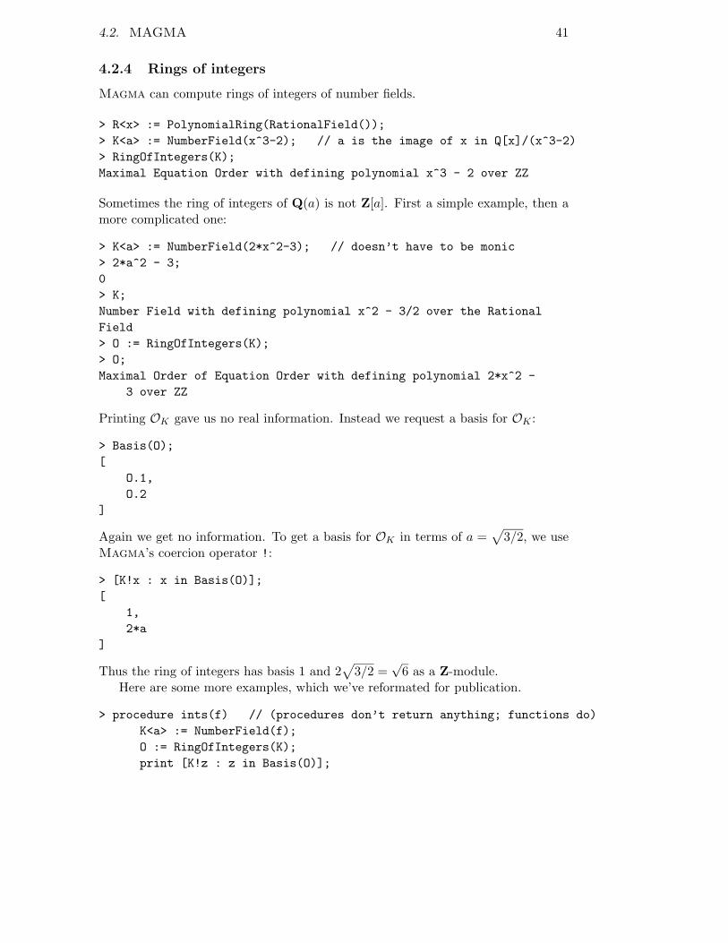
4.2.4 Rings of integers

Magma can compute rings of integers of number fields.


> K<a> := NumberField(x^3-2); // a is the image of x in Q[x]/(x^3-2)

> RingOfIntegers(K);

Maximal Equation Order with defining polynomial x^3 - 2 over ZZ

Sometimes the ring of integers of Q(a) is not Z[a]. First a simple example, then amore complicated one:

> K<a> := NumberField(2*x^2-3); // doesn’t have to be monic

> 2*a^2 - 3;

0

> K;

Number Field with defining polynomial x^2 - 3/2 over the Rational

Field

> O := RingOfIntegers(K);

> O;

Maximal Order of Equation Order with defining polynomial 2*x^2 -

3 over ZZ

Printing OK gave us no real information. Instead we request a basis for OK :

> Basis(O);

[

O.1,

O.2

]

Again we get no information. To get a basis for OK in terms of a =√

3/2, we useMagma’s coercion operator !:

> [K!x : x in Basis(O)];

[

1,

2*a

]

Thus the ring of integers has basis 1 and 2√

3/2 =√

6 as a Z-module.Here are some more examples, which we’ve reformated for publication.

> procedure ints(f) // (procedures don’t return anything; functions do)

K<a> := NumberField(f);

O := RingOfIntegers(K);

print [K!z : z in Basis(O)];


end procedure;

> ints(x^2-5);

[

1, 1/2*(a + 1)

]

> ints(x^2+5);

[

1, a

]

> ints(x^3-17);

[

1, a, 1/3*(a^2 + 2*a + 1)

]

> ints(CyclotomicPolynomial(7));

[

1, a, a^2, a^3, a^4, a^5

]

> ints(x^5+&+[Random(10)*xî : i in [0..4]]); // RANDOM

[

1, a, a^2, a^3, a^4

]

> ints(x^5+&+[Random(10)*xî : i in [0..4]]); // RANDOM

[

1, a, a^2, 1/2*(a^3 + a),

1/16*(a^4 + 7*a^3 + 11*a^2 + 7*a + 14)

]

Lets find out how high of a degree Magma can easily deal with.

> d := 10; time ints(&+[i*xî + 2*x+1: i in [0..d]]);

[

1, 10*a, ...

]

Time: 0.030


...

Time: 0.160


...

Time: 1.610


...

Time: 0.640


...

4.2. MAGMA 43

Time: 3.510


...

Time: 12.020


...

Time: 34.480


...

Time: 5.580 -- the timings very *drastically* on the same problem,

because presumably some randomized algorithms are used.


...

Time: 70.350


Time: 136.740

Recall that an order is a subring of OK of finite index as an additive group. Wecan also define orders in rings of integers in Magma.



> O := Order([2*a]);

> O;

Transformation of Order over

Equation Order with defining polynomial x^3 - 2 over ZZ

Transformation Matrix:

[1 0 0]

[0 2 0]

[0 0 4]


> Index(OK,O);

8

4.2.5 Ideals

We can construct ideals in rings of integers of number fields in Magma as illustrated.




> I := 7*OK;

> I;

Principal Ideal of OK

Generator:


[7, 0]

> J := (OK!a)*OK; // the ! computes the natural image of a in OK

> J;


Generator:

[-1, 2]

> Generators(J);

[ [-1, 2] ]

> K!Generators(J)[1];

a

> I*J;


Generator:

[-7, 14]

> J*I;


Generator:

[-7, 14]

> I+J;


Generator:

[1, 0]

>

> Factorization(I);

[

<Principal Prime Ideal of OK

Generator:

[7, 0], 1>

]


[


Generator:

[3, 0], 1>

]


[

<Prime Ideal of OK


[5, 0]

[4, 2], 2>

]


4.3. USING PARI 45

[

<Prime Ideal of OK


[11, 0]

[14, 2], 1>,

<Prime Ideal of OK


[11, 0]

[17, 2], 1>

]

We can even work with fractional ideals in Magma.



> I := 7*OK;

> J := (OK!a)*OK;

> M := I/J;

> M;

Fractional Principal Ideal of OK

Generator:

-7/5*OK.1 + 14/5*OK.2

> Factorization(M);

[

<Prime Ideal of OK


[5, 0]

[4, 2], -1>,


Generator:

[7, 0], 1>

]

4.3 Using PARI

PARI is freely available (under the GPL) from

http://pari.math.u-bordeaux.fr/

The above website describes PARI thus:

PARI/GP is a widely used computer algebra system designed for fastcomputations in number theory (factorizations, algebraic number the-ory, elliptic curves...), but also contains a large number of other usefulfunctions to compute with mathematical entities such as matrices, poly-nomials, power series, algebraic numbers etc., and a lot of transcendental


functions. PARI is also available as a C library to allow for faster com-putations.

Originally developed by Henri Cohen and his co-workers (Universit Bor-deaux I, France), PARI is now under the GPL and maintained by KarimBelabas (Universit Paris XI, France) with the help of many volunteercontributors.

The sections below are very similar to the Magma sections above, except theyaddress PARI instead of Magma. We use Pari Version 2.2.9-alpha for all examplesbelow, and all timings are on an Opteron 248.

4.3.1 Smith Normal Form

In Section 2.1 we learned about Smith normal forms of matrices. We create matricesin PARI by giving the entries of each row separated by a ;.

? A = [1,2;3,4];

? A

[1 2]

[3 4]

? matsnf(A)

[2, 1]

The matsnf function computes the diagonal entries of the Smith normal form ofa matrix. To get documentation about a function PARI, type ? followed by thefunction name.

? ?matsnf

matsnf(x,{flag=0}): Smith normal form (i.e. elementary divisors)

of the matrix x, expressed as a vector d. Binary digits of flag

mean 1: returns [u,v,d] where d=u*x*v, otherwise only the diagonal d

is returned,

2: allow polynomial entries, otherwise assume x is integral,

4: removes all information corresponding to entries equal

to 1 in d.

Next, let’s test the limits. To time code in PARI use the gettime function:

? ?gettime

gettime(): time (in milliseconds) since last call to gettime.

If we divide the result of gettime by 1000 we get the time in seconds.We make a 10× 10 integer matrix with random entries between 0 and 100, and

compute its Smith normal form.

> n=10;A=matrix(n,n,i,j,random(101));gettime;B=matsnf(A);gettime/1000.0

%7 = 0.0010000000000000000000000000000000000000

4.3. USING PARI 47

Let’s see how big we have to make A in order to slow down PARI 2.2.9-alpha. Thesetimings below are on an Opteron 248 server.

? n=50;A=matrix(n,n,i,j,random(101));gettime;B=matsnf(A);gettime/1000.0

0.058


1.3920000000000000000000000000000000000


30.731000000000000000000000000000000000


*** matsnf: the PARI stack overflows !

current stack size: 8000000 (7.629 Mbytes)

[hint] you can increase GP stack with allocatemem()

? allocatemem(); allocatemem(); allocatemem()

*** allocatemem: Warning: doubling stack size; new stack = 16000000 (15.259 Mbytes).


35.742000000000000000000000000000000000

Remark 4.3.1. The same timings on a 1.8Ghz Pentium M notebook are 0.189,

5.489, 48.185, 170.21, respectively. On a G5 XServe, they are 0.19, 5.70,

41.95, 153.98, respectively.Recall that the timings for the same computation on the Opteron under Magma

are 0.020, 0.210, 1.240, 4.290, which is vastly faster than PARI.

4.3.2 Number Fields

There are several ways to define number fields in PARI. The simplest is to give amonic integral polynomial as input to the nfinit function.

? K = nfinit(x^3-2);

Number fields do not print as nicely in PARI as in Magma:

? K

K

%12 = [x^3 - 2, [1, 1], -108, 1, [[1, 1.2599210498948731647672106072782283506,

... and tons more numbers! ...

Confusingly, elements of number fields can be represented in PARI in many differ-ent ways. I refer you to the documentation for PARI (§3.6). A simple way is aspolymods:

? a = Mod(x, x^3-2) \\ think of this as x in Q[x]/(x^3-2).

? a

Mod(x, x^3 - 2)

? a^3

Mod(2, x^3 - 2)


4.3.3 Rings of integers

To compute the ring of integers of a number field in PARI, use the nfbasis com-mand.

? ?nfbasis

nfbasis(x,{flag=0},{p}): integral basis of the field Q[a], where a is

a root of the polynomial x, using the round 4 algorithm. Second and

third args are optional. Binary digits of flag means:

1: assume that no square of a prime>primelimit divides the

discriminant of x,

2: use round 2 algorithm instead.

If present, p provides the matrix of a partial factorization of the

discriminant of x, useful if one wants only an order maximal at

certain primes only.

For example, we compute the ring of integers of Q( 3√

2).

? nfbasis(x^3-2)

[1, x, x^2]

? nfbasis(2*x^2-3)

[1, 2*x]

Here are some more examples, which we’ve reformated for publication.

> nfbasis(x^2-5)

[1, 1/2*x + 1/2]

? nfbasis(x^3-17)

[1, x, 1/3*x^2 - 1/3*x + 1/3]

? nfbasis(polcyclo(7))

[1, x, x^2, x^3, x^4, x^5]

? d=10; f=sum(i=0,d,i*x^i+2*x+1); gettime; nfbasis(f); gettime/1000.0

0.011000000000000000000000000000000000000


0.027000000000000000000000000000000000000


1.6690000000000000000000000000000000000


1.6640000000000000000000000000000000000


0.080000000000000000000000000000000000000


1.5000000000000000000000000000000000000


12.288000000000000000000000000000000000

4.3. USING PARI 49


1.6380000000000000000000000000000000000


38.141000000000000000000000000000000000


33.423000000000000000000000000000000000


33.066000000000000000000000000000000000 \\ doesn’t vary much

Lets find out how high of a degree PARI can easily deal with.

Recall that the timing in Magma for computing OK for d = 30 was 136.740seconds, which is four times as long as the 33 second timing of PARI.1 Thus forthe fields considered above, computation of OK in PARI is faster than in MAGMA.Sometimes one system is much better than another, and it is not clear a priori whichwill be better.

4.3.4 Ideals

In PARI ideals can be represented in several ways. For example, to construct aprincipal ideal, give the generator. There is no ideal data type, but you can givedata that defines an ideal, e.g., an alement to define a principal ideal, to functionsthat take ideals as input.

The following examples illustrate basic arithmetic with ideals and factorizationof ideals.

? a = Mod(x, x^2-5)

%41 = Mod(x, x^2 - 5)

? nf = nfinit(x^2-5);

? idealadd(nf, 5*a, 10*a)

%44 =

[25 15]

[ 0 5]

The output of idealadd is a 2-column matrix, whose columns represent elementsof K on the integral basis for OK output by nfbasis. These two elements generatethe ideal as an OK-module. We will prove later (see Prop. 6.3.2) that every idealcan be generated by 2 elements.

Note that fractional ideals are also allowed:

1I onced discussed timings of PARI versus Magma with John Cannon, who is the director ofMagma. He commented that in some cases PARI implicitly assumes unproven conjectures, e.g.,the Riemann Hypothesis, in order to get such fast algorithms, whereas the philosophy in Magma

is to not assume conjectures unless one explicitly asks it to.


? idealadd(nf, a/5, 10*a)

%45 =

[1 3/5]

[0 1/5]

We can also factor an ideal as a product of prime ideals. The output is anarrays of pairs, a prime ideal and its exponent. These ideals are represented in yetanother way, as a 5-tuple [p, a, e, f, b], where a is a vector of integers. Such a tuplecorresponds to the ideal pOK + αOK , where α =

∑aiωi, and the ωi are the basis

output by nfbasis. Explaining e, f, b requires ideas that we have not yet introduced(ramification, inertia degrees, etc.) Here are some examples:

? nf = nfinit(x^2-5);

? idealfactor(nf, 7)

%46 =

[[7, [7, 0]~, 1, 2, [1, 0]~] 1]


%47 =

[[3, [3, 0]~, 1, 2, [1, 0]~] 1]


%48 =

[[5, [1, 2]~, 2, 1, [1, 2]~] 2]


%49 =

[[11, [-3, 2]~, 1, 1, [5, 2]~] 1]

[[11, [5, 2]~, 1, 1, [-3, 2]~] 1]

We can even factor fractional ideals:

? idealfactor(nf, 1/11)

%50 =

[[11, [-3, 2]~, 1, 1, [5, 2]~] -1]

[[11, [5, 2]~, 1, 1, [-3, 2]~] -1]

Chapter 5

Factoring Primes

Let p be a prime and OK the ring of integers of a number field. This chapter is abouthow to write pOK as a product of prime ideals of OK . Paradoxically, computingthe explicit prime ideal factorization of pOK is easier than computing OK .

5.1 The Problem

A diagram from [LL93].

“The obvious mathematical breakthrough would be develop-ment of an easy way to factor large prime numbers.”

– Bill Gates, The Road Ahead, 1st ed., pg 265

51

52 CHAPTER 5. FACTORING PRIMES

Bill Gates meant1 factoring products of two primes, which would break the RSAcryptosystem (see e.g. [Ste, §3.2]). However, perhaps he really meant what he said:then we might imagine that he meant factorization of primes of Z in rings of integersof number fields. For example, 216 + 1 = 65537 is a “large” prime, and in Z[i] wehave (65537) = (65537, 28 + i) · (65537, 28 − i).

5.1.1 Geomtric Intuition

Let K = Q(α) be a number field, and let OK be the ring of integers of K. Toemploy our geometric intuition, as the Lenstras did on the cover of [LL93], it ishelpful to view OK as a one-dimensional scheme

X = Spec(OK) = { all prime ideals of OK }

over

Y = Spec(Z) = {(0)} ∪ {pZ : p ∈ Z>0 is prime }.There is a natural map π : X → Y that sends a prime ideal p ∈ X to p ∩ Z ∈ Y .For example, if

p = (65537, 28 + i) ⊂ Z[i],

then p ∩ Z = (65537). For more on this viewpoint, see [Har77] and [EH00, Ch. 2].If p ∈ Z is a prime number, then the ideal pOK of OK factors uniquely as

a product∏

pei

i , where the pi are maximal ideals of OK . We may imagine thedecomposition of pOK into prime ideals geometrically as the fiber π−1(pZ), wherethe exponents ei are the multiplicities of the fibers. Notice that the elements ofπ−1(pZ) are the prime ideals of OK that contain p, i.e., the primes that dividepOK .

This chapter is about how to compute the pi and ei.

5.1.2 Examples

The following Magma session shows the commands needed to compute the factor-ization of pOK in Magma for K the number field defined by a root of x5 + 7x4 +3x2 − x + 1 and p = 2 and 5 (see Section 5.4 for PARI versions):


> K<a> := NumberField(x^5 + 7*x^4 + 3*x^2 - x + 1);


> [K!OK.i : i in [1..5]];

1This quote is on page 265 of the first edition. In the second edition, on page 303, this sentence ischanged to “The obvious mathematical breakthrough that would defeat our public key encryptionwould be the development of an easy way to factor large numbers.” This is less nonsensical;however, fast factoring is not known to break all commonly used public-key cryptosystem. Forexample, there are cryptosystems based on the difficulty of computing discrete logarithms in F

∗

p

and on elliptic curves over Fp, which (presumably) would not be broken even if one could factorlarge numbers quickly.

5.1. THE PROBLEM 53

[ 1, a, a^2, a^3, a^4 ]

> I := 2*OK;

> Factorization(I);

[ <Principal Prime Ideal of OK

Generator: [2, 0, 0, 0, 0], 1>]

> J := 5*OK;

> Factorization(J);

[ <Prime Ideal of OK


[5, 0, 0, 0, 0]

[2, 1, 0, 0, 0], 1>,

<Prime Ideal of OK


[5, 0, 0, 0, 0]

[3, 1, 0, 0, 0], 2>,

<Prime Ideal of OK


[5, 0, 0, 0, 0]

[2, 4, 1, 0, 0], 1>]

Thus 2OK is already a prime ideal, and

5OK = (5, 2 + a) · (5, 3 + a)2 · (5, 2 + 4a + a2).

Notice that in this example OK = Z[a]. (Warning: There are examples of OK

such that OK 6= Z[a] for any a ∈ OK , as Example 5.3.2 below illustrates.) WhenOK = Z[a] it is relatively easy to factor pOK , at least assuming one can factorpolynomials in Fp[x]. The following factorization gives a hint as to why:

x5 + 7x4 + 3x2 − x + 1 ≡ (x + 2) · (x + 3)2 · (x2 + 4x + 2) (mod 5).

The exponent 2 of (5, 3 + a)2 in the factorization of 5OK above suggests “rami-fication”, in the sense that the cover X → Y has less points (counting their “size”,i.e., their residue class degree) in its fiber over 5 than it has generically:


��

��

��

��

� ��

��

��

� ��

� ��

��

��

��

(5, 2 + 4a + a2)

(5, 3 + a)2

(5, 2 + a)

5Z

2OK

2Z

(0)

(0)

3Z 7Z 11Z

Diagram of Spec(OK) → Spec(Z)

5.2 A Method for Factoring Primes that Often Works

Suppose a ∈ OK is such that K = Q(a), and let f(x) ∈ Z[x] be the minimalpolynomial of a. Then Z[a] ⊂ OK , and we have a diagram of schemes

⋃Spec(OK/p

ei

i ) Â

Ä

//

²²

Spec(OK)

²²⋃Spec(Fp[x]/(f

ei

i )) Â

Ä

//

²²

Spec(Z[a])

²²Spec(Fp)

Â

Ä

// Spec(Z)

where f =∏

i fei

i is the factorization of the image of f in Fp[x], and pOK =∏

pei

i

is the factorization of pOK in terms of prime ideals of OK . On the level of rings,the bottom horizontal map is the quotient map Z → Z/pZ ∼= Fp. The middle

5.2. A METHOD FOR FACTORING PRIMES THAT OFTEN WORKS 55

horizontal map is induced by

Z[x] →⊕

i

Fp[x]/(fei

i ),

and the top horizontal map is induced by

OK → OK/pOK∼=

⊕OK/p

ei

i ,

where the isomorphism is by the Chinese Remainder Theorem, which we will provein Chapter 6. The left vertical maps come from the inclusions

Fp ↪→ Fp[x]/(fei

i ) ↪→ OK/pei

i ,

and the right from the inclusions Z ↪→ Z[a] ↪→ OK .

The cover π : Spec(Z[a]) → Spec(Z) is easy to understand because it is definedby the single equation f(x), in the sense that Z[a] ∼= Z[x]/(f(x)). To give a maximalideal p of Z[a] such that π(p) = pZ is the same as giving a homomorphism ϕ :Z[x]/(f) → Fp up to automorphisms of the image, which is in turn the same asgiving a root of f in Fp up to automorphism, which is the same as giving anirreducible factor of the reduction of f modulo p.

Lemma 5.2.1. Suppose the index of Z[a] in OK is coprime to p. Then the primes pi

in the factorization of pZ[a] do not decompose further going from Z[a] to OK , sofinding the prime ideals of Z[a] that contain p yields the primes that appear in thefactorization of pOK .

Proof. Fix a basis for OK and for Z[a] as Z-modules. Form the matrix A whosecolumns express each basis element of Z[a] as a Z-linear combination of the basisfor OK . Then

det(A) = ±[OK : Z[a]]

is coprime to p, by hypothesis. Thus the reduction of A modulo p is invertible, soit defines an isomorphism Z[a]/pZ[a] ∼= OK/pOK .

Let Fp denote a fixed algebraic closure of Fp; thus Fp is an algebraically closedfield of characteristic p, over which all polynomials in Fp[x] factor into linear fac-tors. Any homomorphism OK → Fp send p to 0, so is the composition of ahomomorphism OK → OK/pOK with a homomorphism OK/pOK → Fp. SinceOK/pOK

∼= Z[a]/pZ[a], the homomorphisms OK → Fp are in bijection with thehomomorphisms Z[a] → Fp. The homomorphisms Z[a] → Fp are in bijection withthe roots of the reduction modulo p of the minimal polynomial of a in Fp.

Remark 5.2.2. Here is a “high-brow” proof of Lemma 5.2.1. By hypothesis we havean exact sequence of abelian groups

0 → Z[a] → OK → H → 0,


where H is a finite abelian group of order coprime to p. Tensor product is rightexact, and there is an exact sequence

Tor1(H,Fp) → Z[a] ⊗ Fp → OK ⊗ Fp → H ⊗ Fp → 0,

and Tor1(H,Fp) = H ⊗ Fp = 0, so Z[a] ⊗ Fp∼= OK ⊗ Fp.

As suggested in the proof of the lemma, we find all homomorphisms OK → Fp

by finding all homomorphism Z[a] → Fp. In terms of ideals, if p = (f(a), p)Z[a] is amaximal ideal of Z[a], then the ideal p′ = (f(a), p)OK of OK is also maximal, since

OK/p′ ∼= (OK/pOK)/(f(a)) ∼= (Z[a]/pZ[a])/(f(a)) ⊂ Fp,

where a denotes the image of a in OK/pOK .

We formalize the above discussion in the following theorem (note: we will notprove that the powers are ei here):

Theorem 5.2.3. Let f ∈ Z[x] be the minimal polynomial of a over Z. Supposethat p - [OK : Z[a]] is a prime. Let

f =

t∏

i=1

fei

i ∈ Fp[x]

where the f i are distinct monic irreducible polynomials. Let pi = (p, fi(a)) wherefi ∈ Z[x] is a lift of f i in Fp[X]. Then

pOK =t∏

i=1

pei

i .

We return to the example from above, in which K = Q(a), where a is a rootof f = x5 + 7x4 + 3x2 − x + 1. According to Magma, the ring of integers OK hasdiscriminant 2945785:


> K<a> := NumberField(x^5 + 7*x^4 + 3*x^2 - x + 1);

> Discriminant(RingOfIntegers(K));

2945785

The order Z[a] has the same discriminant as f(x), which is the same as the dis-criminant of OK , so Z[a] = OK and we can apply the above theorem. (Here we usethat the index of Z[a] in OK is the square of the quotient of their discriminants, afact we will prove later in Section 7.2.)

> Discriminant(x^5 + 7*x^4 + 3*x^2 - x + 1);

2945785

5.3. A GENERAL METHOD 57

We have

x5 + 7x4 + 3x2 − x + 1 ≡ (x + 2) · (x + 3)2 · (x2 + 4x + 2) (mod 5),

which yields the factorization of 5OK given before the theorem.

If we replace a by b = 7a, then the index of Z[b] in OK will be a power of 7,which is coprime to 5, so the above method will still work.

> f := MinimalPolynomial(7*a);

> f;

x^5 + 49*x^4 + 1029*x^2 - 2401*x + 16807

> Discriminant(f);

235050861175510968365785

> Discriminant(f)/Discriminant(RingOfIntegers(K));

79792266297612001 // coprime to 5

> S<t> := PolynomialRing(GF(5));

> Factorization(S!f);

[ <t + 1, 2>,

<t + 4, 1>,

<t^2 + 3*t + 3, 1> ]

Thus 5 factors in OK as

5OK = (5, 7a + 1)2 · (5, 7a + 4) · (5, (7a)2 + 3(7a) + 3).

If we replace a by b = 5a and try the above algorithm with Z[b], then the methodfails because the index of Z[b] in OK is divisible by 5.

> f := MinimalPolynomial(5*a);

> f;

x^5 + 35*x^4 + 375*x^2 - 625*x + 3125

> Discriminant(f) / Discriminant(RingOfIntegers(K));

95367431640625 // divisible by 5

> Factorization(S!f);

[ <t, 5> ]

5.3 A General Method

There are numbers fields K such that OK is not of the form Z[a] for any a ∈ K.Even worse, Dedekind found a field K such that 2 | [OK : Z[a]] for all a ∈ OK , sothere is no choice of a such that Theorem 5.2.3 can be used to factor 2 for K (seeExample 5.3.2 below).


5.3.1 Essential Discriminant Divisors

Definition 5.3.1. A prime p is an essential discriminant divisor if p | [OK : Z[a]]for every a ∈ OK .

See Example 7.2.5 below for why is it called an essential “discriminant” insteadof an essential “index divisor”.

Since [OK : Z[a]]2 is the absolute value of Disc(f(x))/ Disc(OK), where f(x) isthe characteristic polynomial of f(x), an essential discriminant divisor divides thediscriminant of the characteristic polynomial of any element of OK .

Example 5.3.2 (Dedekind). Let K = Q(a) be the cubic field defined by a root a ofthe polynomial f = x3 +x2−2x+8. We will use Magma, which implements the al-gorithm described in the previous section, to show that 2 is an essential discriminantdivisor for K.

> K<a> := NumberField(x^3 + x^2 - 2*x + 8);



[ <Prime Ideal of OK

Basis:

[2 0 0]

[0 1 0]

[0 0 1], 1>,

<Prime Ideal of OK

Basis:

[1 0 1]

[0 1 0]

[0 0 2], 1>,

<Prime Ideal of OK

Basis:

[1 0 1]

[0 1 1]

[0 0 2], 1> ]

Thus 2OK = p1p2p3, with the pi distinct, and one sees directly from the aboveexpressions that OK/pi

∼= F2. If OK = Z[a] for some a ∈ OK with minimalpolynomial f , then f(x) ∈ F2[x] must be a product of three distinct linear factors,which is impossible, since the only linear polynomials in F2[x] are x and x + 1.

5.3.2 Remarks on Ideal Factorization in General

Recall (from Definition 2.3.10) that an order in OK is a subring O of OK that hasfinite index in OK . For example, if OK = Z[i], then O = Z + 5Z[i] is an order inOK , and as an abelian group OK/O is cyclic of order 5.

Most algebraic number theory books do not describe an algorithm for decom-posing primes in the general case. Fortunately, Cohen’s book [Coh93, Ch. 6] does

5.3. A GENERAL METHOD 59

describe how to solve the general problem, in more than one way. The algorithmsare nontrivial, and occupy a substantial part of Chapter 6 of Cohen’s book. Ourgoal for the rest of this section is to give a hint as to what goes into them.

The general solutions to prime ideal factorization are somewhat surprising,since the algorithms are much more sophisticated than the one suggested by Theo-rem 5.2.3. However, these complicated algorithms all run very quickly in practice,even without assuming the maximal order is already known. In fact, they avoidcomputing OK altogether, and instead compute only an order O that is p-maximal,i.e., is such that p - [OK : O].

For simplicity we consider the following slightly easier problem whose solutionillustrates the key ideas needed in the general case.

Problem 5.3.3. Let O be any order in OK and let p be a prime of Z. Find theprime ideals of O that contain p.

Given a prime p that we wish to factor in OK , we first find a p-maximal order O.We then use a solution to Problem 5.3.3 to find the prime ideals p of O that containp. Second, we find the exponents e such that pe exactly divides pO. The resultingfactorization in O completely determines the factorization of pOK .

A p-maximal order can be found reasonably quickly in practice using algorithmscalled “round 2” and “round 4”. To compute OK , given an order Z[α] ⊂ OK , onetakes a sum of p-maximal orders, one for every p such that p2 divides Disc(Z[α]).The time-consuming part of this computation is finding the primes p such thatp2 | Disc(Z[α]), not finding the p-maximal orders. This example illustrates that afast algorithm for factoring integers would not only break the RSA cryptosystems,but would massively speed up computation of the ring of integers of a number field.

Remark 5.3.4. The MathSciNet review of [BL94] by J. Buhler contains the following:

A result of Chistov says that finding the ring of integers OK in analgebraic number field K is equivalent, under certain polynomial timereductions, to the problem of finding the largest squarefree divisor of apositive integer. No feasible (i.e., polynomial time) algorithm is knownfor the latter problem, and it is possible that it is no easier than themore general problem of factoring integers.

Thus it appears that computing the ring OK is quite hard.

5.3.3 Finding a p-Maximal Order

Before describing the general factorization algorithm, we sketch some of the theorybehind the general algorithms for computing a p-maximal order O in OK . The maininput is the following theorem, whose proof can be found in [Coh93, §6.1.1].

Theorem 5.3.5 (Pohst-Zassenhaus). Let O be an order in the the ring of inte-gers OK of a number field, let p ∈ Z be a prime, and let

Ip = {x ∈ O : xm ∈ pO for some m ≥ 1 } ⊂ O


be the radical of pO, which is an ideal of O. Let

O′ = {x ∈ K : xIp ⊂ Ip}.

Then O′ is an order and either O′ = O, in which case O is p-maximal, or O ⊂ O′

and p divides [O′ : O].

After deciding on how to represent elements of K and orders and ideals in K,one can give an efficient algorithm to compute the O′ of the theorem. The algorithmmainly involves linear algebra over finite fields. It is complicated to describe, butefficient in practice, and is conceptually simple—just compute O′. The trick forreducing the computation of O′ to linear algebra is the following lemma:

Lemma 5.3.6. Define a homomorphism map ψ : O ↪→ End(Ip/pIp) given by send-ing α ∈ O to left multiplication by the reduction of α modulo p. Then

O′ =1

pKer(ψ).

Note that to give an algorithm one must also figure out how to compute Ip/pIp

and the kernel of this map. This is all done in [Coh93, §6.1].

5.3.4 General Factorization Algorithm

We finally give an algorithm to factor pOK in general.

Algorithm 5.3.7 (General Factorization). Let K = Q(a) be a number field givenby an algebraic integer a as a root of its minimal monic polynomial f of degree n. Weassume that an order O has been given by a basis w1, . . . , wn and that O that containsZ[a]. For any prime p ∈ Z, the following algorithm computes the set of maximal idealsof O that contain p.

1. [Check if easy] If p - disc(Z[a])/ disc(O) (so p - [O : Z[a]]), then using Theo-rem 5.2.3 we factor pO.

2. [Compute radical] Let I be the radical of pO, which is the ideal of elements x ∈ Osuch that xm ∈ pO for some positive integer m. Note that pO ⊂ I, i.e., I | pO;also I is the product of the primes that divide p, without multiplicity. Using linearalgebra over the finite field Fp, we compute a basis for I/pO, hence I, sincepO ⊂ I.

3. [Compute quotient by radical] Compute an Fp basis for

A = O/I = (O/pO)/(I/pO).

The second equality comes from the fact that pO ⊂ I. Note that O/pO isobtained by simply reducing the basis w1, . . . , wn modulo p.

5.4. APPENDIX: THE CALCULATIONS IN PARI 61

4. [Decompose quotient] The ring A decomposes as a product A ∼=∏

Fp[x]/(gi(x))of fields. We can find such a decomposition explicitly using linear algebra.

5. [Compute the maximal ideals over p] Each maximal ideal pi lying over p is thekernel of one of the compositions O → A → Fp[x]/(gi(x)).

Algorithm 5.3.7 finds all primes of O that contain the radical I of pO. Everysuch prime clearly contains p, so to see that the algorithm is correct, we prove thatthe primes p of O that contain p also contain I. If p is a prime of O that contains p,then pO ⊂ p. If x ∈ I then xm ∈ pO for some m, so xm ∈ p which implies thatx ∈ p by primality of p. Thus p contains I, as required. Note that we do not find thepowers of primes that divide p in Algorithm 5.3.7; that’s left to another algorithmthat we will not discuss in this book.

Algorithm 5.3.7 was invented by J. Buchmann and H. W. Lenstra, though theirpaper seems to have never been published; however, the algorithm is described indetail in [Coh93, §6.2.5]. Incidentally, this chapter is based on Chapters 4 and 6 of[Coh93], which is highly recommended, and goes into much more detail about thesealgorithms.

5.4 Appendix: The Calculations in PARI

In this section we give PARI versions of all the Magma calculations in the rest ofthis chapter.

? K = nfinit(x^5 + 7*x^4 + 3*x^2 - x + 1);

? idealfactor(K, 2)

[[2, [2, 0, 0, 0, 0]~, 1, 5, [1, 0, 0, 0, 0]~] 1]

? idealfactor(K, 5)

[[5, [-3, 0, 0, 1, 0]~, 2, 1, [1, 0, 2, -2, -1]~] 2]

[[5, [1, 0, 0, 1, 0]~, 1, 1, [1, 0, -2, 2, -1]~] 1]

[[5, [10, 1, 0, -8, 1]~, 1, 2, [2, 1, 1, -1, 1]~] 1]

? K.disc

2945785

? poldisc(x^5 + 7*x^4 + 3*x^2 - x + 1)

2945785

? a = Mod(x, x^5 + 7*x^4 + 3*x^2 - x + 1);

? f = charpoly(7*a)

x^5 + 49*x^4 + 1029*x^2 - 2401*x + 16807

? poldisc(f)

235050861175510968365785

? poldisc(f)/K.disc

79792266297612001


? factormod(f,5)

[Mod(1, 5)*x + Mod(1, 5) 2]

[Mod(1, 5)*x + Mod(4, 5) 1]

[Mod(1, 5)*x^2 + Mod(3, 5)*x + Mod(3, 5) 1]

? f = charpoly(5*a)

? factormod(f,5)

[Mod(1, 5)*x 5]

? K = nfinit(x^3 + x^2 - 2*x + 8);

? idealfactor(K,2)

[[2, [1, 0, 1]~, 1, 1, [0, 0, -1]~] 1]

[[2, [1, 1, 0]~, 1, 1, [0, 1, 0]~] 1]

[[2, [2, 1, 1]~, 1, 1, [1, 1, 1]~] 1]

Chapter 6

The Chinese Remainder

Theorem

We prove the Chinese Remainder Theorem (CRT) for commutative rings and discusshow to compute with it explicitly in Magma and PARI. We also apply the ChineseRemainder Theorem to prove that every ideal in OK is generated by two elementsand determine the structure of pn/pn+1, where p is a nonzero prime ideal of OK .

6.1 The Chinese Remainder Theorem

6.1.1 CRT in the Integers

The Chinese Remainder Theorem from elementary number theory asserts that ifn1, . . . , nr are integers that are coprime in pairs, and a1, . . . , ar are integers, thenthere exists an integer a such that a ≡ ai (mod ni) for each i = 1, . . . , r. Here“coprime in pairs” means that gcd(ni, nj) = 1 whenever i 6= j; it does not meanthat gcd(n1, . . . , nr) = 1, though it implies this. In terms of rings, the ChineseRemainder Theorem (CRT) asserts that the natural map

Z/(n1 · · ·nr)Z → (Z/n1Z) ⊕ · · · ⊕ (Z/nrZ) (6.1.1)

that sends a ∈ Z to its reduction modulo each ni, is an isomorphism.

This map is not an isomorphism if the ni are not coprime. Indeed, the cardinalityof the left hand side of (6.1.1) is lcm(n1, . . . , nr), whereas the cardinality of the righthand side is n1 · · ·nr.

The isomorphism (6.1.1) can alternatively be viewed as asserting that any systemof linear congruences

x ≡ a1 (mod n1), x ≡ a2 (mod n2), · · · , x ≡ ar (mod nr)

with pairwise coprime moduli has a unique solution modulo n1 . . . nr.

63

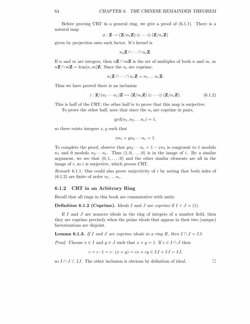
64 CHAPTER 6. THE CHINESE REMAINDER THEOREM

Before proving CRT in a general ring, we give a proof of (6.1.1). There is anatural map

φ : Z → (Z/n1Z) ⊕ · · · ⊕ (Z/nrZ)

given by projection onto each factor. It’s kernel is

n1Z ∩ · · · ∩ nrZ.

If n and m are integers, then nZ ∩ mZ is the set of multiples of both n and m, sonZ ∩ mZ = lcm(n, m)Z. Since the ni are coprime,

n1Z ∩ · · · ∩ nrZ = n1 . . . nrZ.

Thus we have proved there is an inclusion

i : Z/(n1 · · ·nr)Z ↪→ (Z/n1Z) ⊕ · · · ⊕ (Z/nrZ). (6.1.2)

This is half of the CRT; the other half is to prove that this map is surjective.To prove the other half, note that since the ni are coprime in pairs,

gcd(n1, n2 . . . nr) = 1,

so there exists integers x, y such that

xn1 + yn2 · · ·nr = 1.

To complete the proof, observe that yn2 · · ·nr = 1 − xn1 is congruent to 1 modulon1 and 0 modulo n2 · · ·nr. Thus (1, 0, . . . , 0) is in the image of i. By a similarargument, we see that (0, 1, . . . , 0) and the other similar elements are all in theimage of i, so i is surjective, which proves CRT.

Remark 6.1.1. One could also prove surjectivity of i by noting that both sides of(6.1.2) are finite of order n1 . . . nr.

6.1.2 CRT in an Arbitrary Ring

Recall that all rings in this book are commutative with unity.

Definition 6.1.2 (Coprime). Ideals I and J are coprime if I + J = (1).

If I and J are nonzero ideals in the ring of integers of a number field, thenthey are coprime precisely when the prime ideals that appear in their two (unique)factorizations are disjoint.

Lemma 6.1.3. If I and J are coprime ideals in a ring R, then I ∩ J = IJ .

Proof. Choose x ∈ I and y ∈ J such that x + y = 1. If c ∈ I ∩ J then

c = c · 1 = c · (x + y) = cx + cy ∈ IJ + IJ = IJ,

so I ∩ J ⊂ IJ . The other inclusion is obvious by definition of ideal.

6.2. COMPUTING USING THE CRT 65

Lemma 6.1.4. Suppose I1, . . . , Is are pairwise coprime ideals. Then I1 is coprimeto the product I2 · · · Is.

Proof. It suffices to prove the lemma in the case s = 3, since the general case thenfollows from induction. By assumption, there are x1 ∈ I1, y1 ∈ I2 and x2 ∈ I1, y2 ∈I3 such

x1 + y1 = 1 and x2 + y2 = 1.

Multiplying these two relations yields

x1x2 + x1y2 + y1x2 + y1y2 = 1 · 1 = 1.

The first three terms are in I1 and the last term is in I2∩ I3 = I2I3, so I1 is coprimeto I2I3.

Next we prove the Chinese Remainder Theorem in a very general form. We willapply this result with R = OK in the rest of this chapter.

Theorem 6.1.5 (Chinese Remainder Theorem). Suppose I1, . . . , Ir are nonzeroideals of a ring R such Im and In are coprime for any m 6= n. Then the naturalhomomorphism R → ⊕r

n=1 R/In induces an isomorphism

ψ : R/r∏

n=1

In →r⊕

n=1

R/In.

Thus given any an ∈ R, for n = 1, . . . , r, there exists some a ∈ R such that a ≡ an

(mod In) for n = 1, . . . , r; moreover, a is unique modulo∏r

n=1 In.

Proof. Let ϕ : R → ⊕rn=1 R/In be the natural map induced by reduction modulo

the In. An inductive application of Lemma 6.1.3 implies that the kernel ∩rn=1In

of ϕ is equal to∏r

n=1 In, so the map ψ of the theorem is injective.Each projection R → R/In is surjective, so to prove that ψ is surjective, it

suffices to show that (1, 0, . . . , 0) is in the image of ϕ, and similarly for the otherfactors. By Lemma 6.1.4, J =

∏rn=2 In is coprime to I1, there exists x ∈ I1 and

y ∈ J such that x + y = 1. Then y = 1 − x maps to 1 in R/I1 and to 0 in R/J ,hence to 0 in R/In for each n ≥ 2, since J ⊂ In.

6.2 Computing Using the CRT

In order to explicitly compute an a as given by the Theorem 6.1.5, usually one firstprecomputes elements v1, . . . , vr ∈ R such that v1 7→ (1, 0, . . . , 0), v2 7→ (0, 1, . . . , 0),etc. Then given any an ∈ R, for n = 1, . . . , r, we obtain an a ∈ R with an ≡ a(mod In) by taking

a = a1v1 + · · · + arvr.

How to compute the vi depends on the ring R. It reduces to the following problem:Given coprimes ideals I, J ⊂ R, find x ∈ I and y ∈ J such that x + y = 1. If


R is torsion free and of finite rank as a Z-module, so R ≈ Zn, then I, J can berepresented by giving a basis in terms of a basis for R, and finding x, y such thatx+y = 1 can then be reduced to a problem in linear algebra over Z. More precisely,let A be the matrix whose columns are the concatenation of a basis for I with abasis for J . Suppose v ∈ Zn corresponds to 1 ∈ Zn. Then finding x, y such thatx + y = 1 is equivalent to finding a solution z ∈ Zn to the matrix equation Az = v.This latter linear algebra problem can be solved using Hermite normal form (see[Coh93, §4.7.1]), which is a generalization of Gauss elimination.

We next describe how to use Magma and PARI to do CRT computations.

6.2.1 Magma

The Magma command ChineseRemainderTheorem implements the algorithm sug-gested by Theorem 6.1.5. In the following example, we compute a prime over (3)and a prime over (5) of the ring of integers of Q( 3

√2), and find an element of OK

that is congruent to 3√

2 modulo one prime and 1 modulo the other.




> I := Factorization(3*OK)[1][1];

> J := Factorization(5*OK)[1][1];

> I;

Prime Ideal of OK


[3, 0, 0]

[4, 1, 0]

> J;

Prime Ideal of OK


[5, 0, 0]

[7, 1, 0]

> b := ChineseRemainderTheorem(I, J, OK!a, OK!1);

> K!b;

-4

> b - a in I;

true

> b - 1 in J;

true

6.2.2 PARI

There is also a CRT algorithm for number fields in PARI, but it is more cumbersometo use. First we defined Q( 3

√2) and factor the ideals (3) and (5).

6.3. STRUCTURAL APPLICATIONS OF THE CRT 67

? f = x^3 - 2;

? k = nfinit(f);

? i = idealfactor(k,3);

? j = idealfactor(k,5);

Next we form matrix whose rows correspond to a product of two primes, onedividing 3 and one dividing 5:

? m = matrix(2,2);

? m[1,] = i[1,];

? m[1,2] = 1;

? m[2,] = j[1,];

Note that we set m[1,2] = 1, so the exponent is 1 instead of 3. We apply the CRTto obtain a lift in terms of the basis for OK .

? ?idealchinese

idealchinese(nf,x,y): x being a prime ideal factorization and y

a vector of elements, gives an element b such that

v_p(b-y_p)>=v_p(x) for all prime ideals p dividing x,

and v_p(b)>=0 for all other p.

? idealchinese(k, m, [x,1])

[0, 0, -1]~

? nfbasis(f)

[1, x, x^2]

Thus PARI finds the lift −( 3√

2)2, and we finish by verifying that this lift is correct.I couldn’t figure out how to test for ideal membership in PARI, so here we justcheck that the prime ideal plus the element is not the unit ideal, which since theideal is prime, implies membership.

? idealadd(k, i[1,1], -x^2 - x)

[3 1 2]

[0 1 0]

[0 0 1]

? idealadd(k, j[1,1], -x^2-1)

[5 2 1]

[0 1 0]

[0 0 1]

6.3 Structural Applications of the CRT

The next lemma is an application of the Chinese Remainder Theorem. We will useit to prove that every ideal of OK can be generated by two elements. Suppose that Iis a nonzero integral ideals of OK . If a ∈ I, then (a) ⊂ I, so I divides (a) and thequotient (a)I−1 is an integral ideal. The following lemma asserts that (a) can bechosen so the quotient (a)I−1 is coprime to any given ideal.


Lemma 6.3.1. If I and J are nonzero integral ideals in OK , then there exists ana ∈ I such that the integral ideal (a)I−1 is coprime to J .

Before we give the proof in general, note that the lemma is trivial when I isprincipal, since if I = (b), just take a = b, and then (a)I−1 = (a)(a−1) = (1) iscoprime to every ideal.

Proof. Let p1, . . . , pr be the prime divisors of J . For each n, let vn be the largestpower of pn that divides I. Since pvn

n 6= pvn+1n , we can choose an element an ∈ pvn

n

that is not in pvn+1n . By Theorem 6.1.5 applied to the r + 1 coprime integral ideals

pv1+11 , . . . , pvr+1

r , I ·(∏

pvnn

)−1,

there exists a ∈ OK such that

a ≡ an (mod pvn+1n )

for all n = 1, . . . , r and also

a ≡ 0 (mod I ·(∏

pvnn

)−1).

To complete the proof we show that (a)I−1 is not divisible by any pn, or equiv-alently, that each pvn

n exactly divides (a). Because a ≡ an (mod pvn+1n ), there is

b ∈ pvn+1n such that a = an + b. Since an ∈ pvn

n , it follows that a ∈ pvnn , so pvn

n

divides (a). If a ∈ pvn+1n , then an = a−b ∈ pvn+1

n , a contradiction, since an 6∈ pvn+1n .

We conclude that pvn+1n does not divide (a), which completes the proof.

Suppose I is a nonzero ideal of OK . As an abelian group OK is free of rank equalto the degree [K : Q] of K, and I is of finite index in OK , so I can be generated as anabelian group, hence as an ideal, by [K : Q] generators. The following propositionasserts something much better, namely that I can be generated as an ideal in OK

by at most two elements.

Proposition 6.3.2. Suppose I is a fractional ideal in the ring OK of integers of anumber field. Then there exist a, b ∈ K such that I = (a, b) = {αa+βb : α, β ∈ OK}.

Proof. If I = (0), then I is generated by 1 element and we are done. If I is not anintegral ideal, then there is x ∈ K such that xI is an integral ideal, and the numberof generators of xI is the same as the number of generators of I, so we may assumethat I is an integral ideal.

Let a be any nonzero element of the integral ideal I. We will show that thereis some b ∈ I such that I = (a, b). Let J = (a). By Lemma 6.3.1, there exists b ∈ Isuch that (b)I−1 is coprime to (a). Since a, b ∈ I, we have I | (a) and I | (b), soI | (a, b). Suppose pn | (a, b) with p prime. Then pn | (a) and pn | (b), so p - (b)I−1,since (b)I−1 is coprime to (a). We have pn | (b) = I · (b)I−1 and p - (b)I−1, so pn | I.Thus (a, b) | I, so I = (a, b), as claimed.

6.3. STRUCTURAL APPLICATIONS OF THE CRT 69

We can also use Theorem 6.1.5 to determine the OK-module structure of pn/pn+1.

Proposition 6.3.3. Let p be a nonzero prime ideal of OK , and let n ≥ 0 be aninteger. Then pn/pn+1 ∼= OK/p as OK-modules.

Proof. 1 Since pn 6= pn+1, by unique factorization, there is an element b ∈ pn suchthat b 6∈ pn+1. Let ϕ : OK → pn/pn+1 be the OK-module morphism defined byϕ(a) = ab. The kernel of ϕ is p since clearly ϕ(p) = 0 and if ϕ(a) = 0 thenab ∈ pn+1, so pn+1 | (a)(b), so p | (a), since pn+1 does not divide (b). Thus ϕinduces an injective OK-module homomorphism OK/p ↪→ pn/pn+1.

It remains to show that ϕ is surjective, and this is where we will use Theo-rem 6.1.5. Suppose c ∈ pn. By Theorem 6.1.5 there exists d ∈ OK such that

d ≡ c (mod pn+1) and d ≡ 0 (mod (b)/pn).

We have pn | (d) since d ∈ pn and (b)/pn | (d) by the second displayed condition, sosince p - (b)/pn, we have (b) = pn · (b)/pn | (d), hence d/b ∈ OK . Finally

ϕ

(d

b

)=

d

b· d (mod pn+1) = b (mod pn+1) = c (mod pn+1),

so ϕ is surjective.

1Proof from [SD01, pg. 13].

Chapter 7

Discrimants and Norms

In this chapter we give a geometric interpretation of the discriminant of an order ina number field. We also define norms of ideals and prove that the norm function ismultiplicative. Discriminants of orders and norms of ideals will play a crucial rollin our proof of finiteness of the class group in the next chapter.

7.1 Field Embeddings

Let K be a number field of degree n. By the primitive element theorem, K =Q(α) for some α, so we can write K ∼= Q[x]/(f), where f ∈ Q[x] is the minimalpolynomial of α. Because C is algebraically closed and f is irreducible, it has exactlyn = [K : Q] complex roots. Each of these roots z ∈ C induces a homomorphismQ[x] → C given by x 7→ z, whose kernel is (f). Thus we obtain n embeddings ofK ∼= Q[x]/(f) into C:

σ1, . . . , σn : K ↪→ C.

Let σ : K ↪→ Cn be the map a 7→ (σ1(a), . . . , σn(a)), and let V = Rσ(K) be theR-span of the image σ(K) of K inside Cn.

Lemma 7.1.1. Suppose L ⊂ Rn is a subgroup of the vector space Rn. Then theinduced topology on L is discrete if and only if for every H > 0 the set

XH = {v ∈ L : max{|v1|, . . . , |vn|} ≤ H}

is finite.

Proof. If L is not discrete, then there is a point x ∈ L such that for every ε > 0there is y ∈ L such that 0 < |x− y| < ε. By choosing smaller and smaller ε, we findinfinitely many elements x−y ∈ L all of whose coordinates are smaller than 1. Theset X(1) is thus not finite. Thus if the sets XH are all finite, L must be discrete.

Next assume that L is discrete and let H > 0 be any positive number. Then forevery x ∈ XH there is an open ball Bx that contains x but no other element of L.Since XH is closed and bounded, it is compact, so the open covering ∪Bx of XH

has a finite subcover, which implies that XH is finite, as claimed.

71

72 CHAPTER 7. DISCRIMANTS AND NORMS

Lemma 7.1.2. If L if a free abelian group that is discrete in a finite-dimensionalreal vector space V and RL = V , then the rank of L equals the dimension of V .

Proof. If x1, . . . , xm ∈ L are a basis for RL, then M = Zx1 + · · · + Zxm hasfinite index in L, since otherwise the quotient L/M would be infinite, so therewould be infinitely many elements of L in a fundamental domain for M , whichby Lemma 7.1.1 would contradict discreteness of L. Thus the rank of L is m =dim(RL), as claimed.

Proposition 7.1.3. The R-vector space V = Rσ(K) spanned by the image σ(K)has dimension n.

Proof. We prove this by showing that the image σ(OK) is discrete. If σ(OK) werenot discrete it would contain elements all of whose coordinates are simultaneouslyarbitrarily small. The norm of an element a ∈ OK is the product of the entries ofσ(a), so the norms of nonzero elements of OK would go to 0. This is a contradiction,since the norms of elements of OK are integers.

Since σ(OK) is discrete in Cn, Lemma 7.1.2 implies that dim(V ) equals therank of σ(OK). Since σ is injective, dim(V ) is the rank of OK , which equals n byProposition 2.4.4.

Since σ(OK) is a lattice in V , the volume of V/σ(OK) is finite. Supposew1, . . . , wn is a basis for OK . Then if A is the matrix whose ith row is σ(wi),then |det(A)| is the volume of V/σ(OK) (take this as the definition of volume).

Example 7.1.4. Let OK = Z[i] be the ring of integers of K = Q(i). Then w1 = 1,w2 = i is a basis for OK . The map σ : K → C2 is given by

σ(a + bi) = (a + bi, a − bi) ∈ C2.

The image σ(OK) is spanned by (1, 1) and (i,−i). The volume determinant is

∣∣∣∣(

1 1i −i

)∣∣∣∣ = | − 2i| = 2.

Let OK = Z[√

2] be the ring of integers of K = Q(√

2). The map σ is

σ(a + b√

2) = (a + b√

2, a − b√

2) ∈ R2,

and

A =

(1 1√2 −

√2

),

which has determinant −2√

2, so the volume of V/σ(OK) is 2√

2.

As the above example illustrates, the volume V/σ(OK) need not be an integer,and it loses sign information. If we consider det(A)2 instead, we obtain a well-defined integer.

7.2. DISCRIMINANTS 73

7.2 Discriminants

Suppose w1, . . . , wn are a basis for OK as a Z-module, which we view as a Q-vector space. Let σ : K ↪→ Cn be the embedding σ(a) = (σ1(a), . . . , σn(a)), whereσ1, . . . , σn are the distinct embeddings of K into C. Let A be the matrix whoserows are σ(w1), . . . , σ(wn). The quantity det(A) depends on the ordering of the wi,and need not be an integer.

If we consider det(A)2 instead, we obtain a number that is a well-defined integer.Note that

det(A)2 = det(AA) = det(A) det(A) = det(A) det(At) = det(AAt)

= det

∑

k=1,...,n

σk(wi)σk(wj)

= det

∑

k=1,...,n

σk(wiwj)

= det(Tr(wiwj)1≤i,j≤n),

so det(A)2 can be defined purely in terms of the trace without mentioning theembeddings σi. Also, changing the basis for OK is the same as left multiplying Aby an integer matrix U of determinant ±1, which does not change the squareddeterminant, since det(UA)2 = det(U)2 det(A)2 = det(A)2. Thus det(A)2 is welldefined, and does not depend on the choice of basis.

If we view K as a Q-vector space, then (x, y) 7→ Tr(xy) defines a bilinear pairingK × K → Q on K, which we call the trace pairing. The following lemma assertsthat this pairing is nondegenerate, so det(Tr(wiwj)) 6= 0 hence det(A) 6= 0.

Lemma 7.2.1. The trace pairing is nondegenerate.

Proof. If the trace pairing is degenerate, then there exists a ∈ K such that forevery b ∈ K we have Tr(ab) = 0. In particularly, taking b = a−1 we see that0 = Tr(aa−1) = Tr(1) = [K : Q] > 0, which is absurd.

Definition 7.2.2 (Discriminant). Suppose a1, . . . , an is any Q-basis of K. Thediscriminant of a1, . . . , an is

Disc(a1, . . . , an) = det(Tr(aiaj)1≤i,j≤n) ∈ Q.

The discriminant Disc(O) of an order O in OK is the discriminant of any basisfor O. The discriminant dK = Disc(K) of the number field K is the discrimimantof OK .

Note that the discriminants defined above are all nonzero by Lemma 7.2.1.

If α ∈ OK with Z[α] of finite index in OK , and f is the minimal polynomialof α, then Disc(f) = Disc(Z[α]). To see this, note that if we choose the basis1, α, . . . , αn−1 for Z[α], then both discriminants are the square of the same Vander-monde determinant.


Remark 7.2.3. Warning: In Magma Disc(K) is defined to be the discriminant ofthe polynomial you happened to use to define K.

> K := NumberField(x^2-5);

> Discriminant(K);

20

> Discriminant(RingOfIntegers(K));

5

In contrast, PARI does the right thing:

? k=nfinit(x^2-5);

? k.disc

5

The following proposition asserts that the discriminant of an order O in OK isbigger than disc(OK) by a factor of the square of the index.

Proposition 7.2.4. Suppose O is an order in OK . Then

Disc(O) = Disc(OK) · [OK : O]2.

Proof. Let A be a matrix whose rows are the images via σ of a basis for OK ,and let B be a matrix whose rows are the images via σ of a basis for O. SinceO ⊂ OK has finite index, there is an integer matrix C such that CA = B, and|det(C)| = [OK : O]. Then

Disc(O) = det(B)2 = det(CA)2 = det(C)2 det(A)2 = [OK : O]2 · Disc(OK).

Example 7.2.5. Let K be a number field and consider the quantity

D(K) = gcd{Disc(α) : α ∈ OK and [OK : Zα] < ∞}.

One might hope that D(K) is equal to the discriminant Disc(OK) of K. Howeverit’s not in general. Recall Example 5.3.2, of the field generated by a root of f =x3 + x2 − 2x + 8. In that example, the discriminant of OK is coprime to 2, but forevery α ∈ OK , we have 2 | [OK : Z[α]]. By Proposition 7.2.4, the discriminant ofZ[α] is divisible by 4 for all α, so Disc(α) is also divisible by 4. This is the sense inwhich 2 is an “essential discriminant divisor”.

This result is enough to give an algorithm for computing OK , albeit a potentiallyslow one. Given K, find some order O ⊂ K, and compute d = Disc(O). Factor d,and use the factorization to write d = s · f2, where f2 is the largest square thatdivides d. Then the index of O in OK is a divisor of f , and we (tediously) canenumerate all rings R with O ⊂ R ⊂ K and [R : O] | f , until we find the largest oneall of whose elements are integral. A much better algorithm is to proceed exactlyas just described, except use the ideas of Section 5.3.3 to find a p-maximal orderfor each prime divisor of f , then add these p-maximal orders together.

7.3. NORMS OF IDEALS 75

Example 7.2.6. Consider the ring OK = Z[(1 +√

5)/2] of integers of K = Q(√

5).The discriminant of the basis 1, a = (1 +

√5)/2 is

Disc(OK) =

∣∣∣∣(

2 11 3

)∣∣∣∣ = 5.

Let O = Z[√

5] be the order generated by√

5. Then O has basis 1,√

5, so

Disc(O) =

∣∣∣∣(

2 00 10

)∣∣∣∣ = 20 = [OK : O]2 · 5,

hence O is not maximal.

Example 7.2.7. Consider the cubic field K = Q( 3√

2), and let O be the order Z[ 3√

2].Relative to the base 1, 3

√2, ( 3

√2)2 for O, the matrix of the trace pairing is

A =

3 0 00 0 60 6 0

.

Thusdisc(O) = det(A) = 108 = 22 · 33.

Suppose we do not know that the ring of integers OK is equal to O. By Proposi-tion 7.2.4, we have

Disc(OK) · [OK : O]2 = 22 · 33,

so 3 | disc(OK), and [OK : O] | 6. Thus to prove O = OK it suffices to provethat O is 2-maximal and 3-maximal, which could be accomplished as described inSection 5.3.3.

7.3 Norms of Ideals

In this section we extend the notion of norm to ideals. This will be helpful inthe next chapter, where we will prove that the group of fractional ideals moduloprincipal fractional ideals of a number field is finite by showing that every ideal isequivalent to an ideal with norm at most some bound. This is enough, because aswe will see below there are only finitely many ideals of bounded norm.

Definition 7.3.1 (Lattice Index). If L and M are two lattices in a vector space V ,then the lattice index [L : M ] is by definition the absolute value of the determinantof any linear automorphism A of V such that A(L) = M .

For example, if L = 2Z and M = 10Z, then

[L : M ] = [2Z : 10Z] = det([5]) = 5,

since 5 multiples 2Z onto 10Z.The lattice index has the following properties:


• If M ⊂ L, then [L : M ] = #(L/M).

• If M, L, N are any lattices in V , then

[L : N ] = [L : M ] · [M : N ].

Definition 7.3.2 (Norm of Fractional Ideal). Suppose I is a fractional ideal ofOK . The norm of I is the lattice index

Norm(I) = [OK : I] ∈ Q≥0,

or 0 if I = 0.

Note that if I is an integral ideal, then Norm(I) = #(OK/I).

Lemma 7.3.3. Suppose a ∈ K and I is an integral ideal. Then

Norm(aI) = |NormK/Q(a)|Norm(I).

Proof. By properties of the lattice index mentioned above we have

[OK : aI] = [OK : I] · [I : aI] = Norm(I) · |NormK/Q(a)|.

Here we have used that [I : aI] = |NormK/Q(a)|, which is because left multiplica-tion `a is an automorphism of K that sends I onto aI, so [I : aI] = |det(`a)| =|NormK/Q(a)|.

Proposition 7.3.4. If I and J are fractional ideals, then

Norm(IJ) = Norm(I) · Norm(J).

Proof. By Lemma 7.3.3, it suffices to prove this when I and J are integral ideals. IfI and J are coprime, then Theorem 6.1.5 (the Chinese Remainder Theorem) impliesthat Norm(IJ) = Norm(I) · Norm(J). Thus we reduce to the case when I = pm

and J = pk for some prime ideal p and integers m, k. By Proposition 6.3.3, which isa consequence of CRT, the filtration of OK/pn given by powers of p has successivequotients isomorphic to OK/p. Thus we see that #(OK/pn) = #(OK/p)n, whichproves that Norm(pn) = Norm(p)n.

We will use the following proposition in the next chapter when we prove finite-ness of class groups.

Proposition 7.3.5. Fix a number field K. Let B be a positive integer. There areonly finitely many integral ideals I of OK with norm at most B.

Proof. An integral ideal I is a subgroup of OK of index equal to the norm of I. If Gis any finitely generated abelian group, then there are only finitely many subgroupsof G of index at most B, since the subgroups of index dividing an integer n are allsubgroups of G that contain nG, and the group G/nG is finite.

Chapter 8

Finiteness of the Class Group

Frequently OK is not a principal ideal domain. This chapter is about a way tounderstand how badly OK fails to be a principal ideal domain. The class group ofOK measures this failure. As one sees in a course on Class Field Theory, the classgroup and its generalizations also yield deep insight into the extensions of K thatare Galois with abelian Galois group.

8.1 The Class Group

Definition 8.1.1 (Class Group). Let OK be the ring of integers of a numberfield K. The class group CK of K is the group of fractional ideals modulo thesugroup of principal fractional ideals (a), for a ∈ K.

Note that if we let Div(OK) denote the group of fractional ideals, then we havean exact sequence

0 → O∗K → K∗ → Div(OK) → CK → 0.

That the class group CK is finite follows from the first part of the following theoremand the fact that there are only finitely many ideals of norm less than a given integer(Proposition 7.3.5).

Theorem 8.1.2 (Finiteness of the Class Group). Let K be a number field.There is a constant Cr,s that depends only on the number r, s of real and pairsof complex conjugate embeddings of K such that every ideal class of OK containsan integral ideal of norm at most Cr,s

√|dK |, where dK = Disc(OK). Thus by

Proposition 7.3.5 the class group CK of K is finite. One can choose Cr,s such thatevery ideal class in CK contains an integral ideal of norm at most

√|dK | ·

(4

π

)s n!

nn.

77

78 CHAPTER 8. FINITENESS OF THE CLASS GROUP

The explicit bound in the theorem is called the Minkowski bound, and it is thebest known general bound, which doesn’t depend on unproven conjectures.

The following two examples illustrate how to apply Theorem 8.1.2 to computeCK in simple cases.

Example 8.1.3. Let K = Q[i]. Then n = 2, s = 1, and |dK | = 4, so the Minkowskibound is

√4 ·

(4

π

)1 2!

22=

4

π< 2.

Thus every fractional ideal is equivalent to an ideal of norm 1. Since (1) is the onlyideal of norm 1, every ideal is principal, so CK is trivial.

Example 8.1.4. Let K = Q(√

10). We have OK = Z[√

10], so n = 2, s = 0,|dK | = 40, and the Minkowski bound is

√40 ·

(4

π

)0

· 2!

22= 2 ·

√10 · 1

2=

√10 = 3.162277 . . . .

Theorem 8.1.2 implies that every ideal class has a representative that is an integralideal of norm 1, 2, or 3. The ideal 2OK is ramified in OK , so

2OK = (2,√

10).

If (2,√

10) were principal, say (α), then α = a + b√

10 would have norm ±2. Thenthe equation

x2 − 10y2 = ±2, (8.1.1)

would have an integer solution. But the squares mod 5 are 0,±1, so (8.1.1) has nosolutions. Thus (2,

√10) defines a nontrivial element of the class group, and it has

order 2 since its square is the principal ideal 2OK . Thus 2 | #CK .To find the integral ideals of norm 3, we factor x2 − 10 modulo 3, and see that

3OK = (3, 2 +√

10) · (3, 4 +√

10).

If either of the prime divisors of 3OK were principal, then the equation x2 −10y2 =±3 would have an integer solution. Since it doesn’t even have one mod 5, the primedivisors of 3OK are both nontrivial elements of the class group. Let

α =4 +

√10

2 +√

10=

1

3· (1 +

√10).

Then

(3, 2 +√

10) · (α) = (3α, 4 +√

10) = (1 +√

10, 4 +√

10) = (3, 4 +√

10),

so the classes over 3 are equal.In summary, we now know that every element of CK is equivalent to one of

(1), (2,√

10), or (3, 2 +√

10).

Thus the class group is a group of order at most 3 that contains an element oforder 2. Thus it must have order 2.

8.1. THE CLASS GROUP 79

Before proving Theorem 8.1.2, we prove a few lemmas. The strategy of theproof is to start with any nonzero ideal I, and prove that there is some nonzeroa ∈ K, with very small norm, such that aI is an integral ideal. Then Norm(aI) =NormK/Q(a)Norm(I) will be small, since NormK/Q(a) is small. The trick is todetermine precisely how small an a we can choose subject to the condition that aIis an integral ideal, i.e., that a ∈ I−1.

Let S be a subset of V = Rn. Then S is convex if whenever x, y ∈ S then theline connecting x and y lies entirely in S. We say that S is symmetric about theorigin if whenever x ∈ S then −x ∈ S also. If L is a lattice in V , then the volumeof V/L is the volume of the compact real manifold V/L, which is the same thing asthe absolute value of the determinant of any matrix whose rows form a basis for L.

Lemma 8.1.5 (Blichfeld). Let L be a lattice in V = Rn, and let S be a boundedclosed convex subset of V that is symmetric about the origin. Assume that Vol(S) ≥2n Vol(V/L). Then S contains a nonzero element of L.

Proof. First assume that Vol(S) > 2n · Vol(V/L). If the map π : 12S → V/L is

injective, then1

2nVol(S) = Vol

(1

2S

)≤ Vol(V/L),

a contradiction. Thus π is not injective, so there exist P1 6= P2 ∈ 12S such that

P1 − P2 ∈ L. By symmetry −P2 ∈ 12S. By convexity, the average 1

2(P1 − P2) of P1

and −P2 is also in 12S. Thus 0 6= P1 − P2 ∈ S ∩ L, as claimed.

Next assume that Vol(S) = 2n · Vol(V/L). Then for all ε > 0 there is 0 6= Qε ∈L ∩ (1 + ε)S, since Vol((1 + ε)S) > Vol(S) = 2n · Vol(V/L). If ε < 1 then the Qε

are all in L∩ 2S, which is finite since 2S is bounded and L is discrete. Hence thereexists nonzero Q = Qε ∈ L ∩ (1 + ε)S for arbitrarily small ε. Since S is closed,Q ∈ L ∩ S.

Lemma 8.1.6. If L1 and L2 are lattices in V , then

Vol(V/L2) = Vol(V/L1) · [L1 : L2].

Proof. Let A be an automorphism of V such that A(L1) = L2. Then A defines anisomorphism of real manifolds V/L1 → V/L2 that changes volume by a factor of|det(A)| = [L1 : L2]. The claimed formula then follows, since [L1 : L2] = |det(A)|,by definition.

Fix a number field K with ring of integers OK .Let σ1, . . . , σr are the real embeddings of K and σr+1, . . . , σr+s are half the

complex embeddings of K, with one representative of each pair of complex conjugateembeddings. Let σ : K → V = Rn be the embedding

σ(x) =(σ1(x), σ2(x), . . . , σr(x),

Re(σr+1(x)), . . . ,Re(σr+s(x)), Im(σr+1(x)), . . . , Im(σr+s(x))),

Note that this σ is not the same as the one at the beginning of Section 7.2.


Lemma 8.1.7.

Vol(V/σ(OK)) = 2−s√|dK |.

Proof. Let L = σ(OK). From a basis w1, . . . , wn for OK we obtain a matrix Awhose ith row is

(σ1(wi), · · · , σr(wi), Re(σr+1(wi)), . . . ,Re(σr+s(wi)), Im(σr+1(wi)), . . . , Im(σr+s(wi)))

and whose determinant has absolute value equal to the volume of V/L. By doingthe following three column operations, we obtain a matrix whose rows are exactlythe images of the wi under all embeddings of K into C, which is the matrix thatcame up when we defined dK = Disc(OK) in Section 7.2.

1. Add i =√−1 times each column with entries Im(σr+j(wi)) to the column

with entries Re(σr+j(wi)).

2. Multiply all columns Im(σr+j(wi)) by −2i, thus changing the determinant by(−2i)s.

3. Add each columns that now has entries Re(σr+j(wi)) + iIm(σr+j(wi)) to thethe column with entries −2iIm(σr+j(wi)) to obtain columns Re(σr+j(wi)) −iIm(σr+j(wi)).

Recalling the definition of discriminant, we see that if B is the matrix constructedby the above three operations, then det(B)2 = dK . Thus

Vol(V/L) = |det(A)| = |(−2i)−s · det(B)| = 2−s√|dK |.

Lemma 8.1.8. If I is a fractional OK-ideal, then σ(I) is a lattice in V , and

Vol(V/σ(I)) = 2−s√|dK | · Norm(I).

Proof. We know that [OK : I] = Norm(I) is a nonzero rational number. Lemma 8.1.7implies that σ(OK) is a lattice in V , since σ(OK) has rank n as abelian group andspans V , so σ(I) is also a lattice in V . For the volume formula, combine Lem-mas 8.1.6–8.1.7 to get

Vol(V/σ(I)) = Vol(V/σ(OK)) · [OK : I] = 2−s√|dK |Norm(I).

Proof of Theorem 8.1.2. Let K be a number field with ring of integers OK , letσ : K ↪→ V ∼= Rn be as above, and let f : V → R be the function defined by

f(x1, . . . , xn) = |x1 · · ·xr · (x2r+1 + x2

(r+1)+s) · · · (x2r+s + x2

n)|.

8.1. THE CLASS GROUP 81

Notice that if x ∈ K then f(σ(x)) = |NormK/Q(x)|, and

f(ax1, . . . , axn) = |a|nf(x1, . . . , xn).

Let S ⊂ V be any closed, bounded, convex, subset with positive volume thatis symmetric with respect to the origin and has positive volume. Since S is closedand bounded,

M = max{f(x) : x ∈ S}

exists.

Suppose I is any fractional ideal of OK . Our goal is to prove that there isan integral ideal aI with small norm. We will do this by finding an appropriatea ∈ I−1. By Lemma 8.1.8,

c = Vol(V/σ(I−1)) = 2−s√|dK | · Norm(I)−1 =

2−s√|dK |

Norm(I).

Let λ = 2 ·(

cv

)1/n, where v = Vol(S). Then

Vol(λS) = λn Vol(S) = 2n c

v· v = 2n · c = 2n Vol(V/I−1),

so by Lemma 8.1.5 there exists 0 6= b ∈ σ(I−1) ∩ λS. Let a ∈ I−1 be such thatσ(a) = b. Since M is the largest norm of an element of S, the largest norm of anelement of σ(I−1) ∩ λS is at most λnM , so

|NormK/Q(a)| ≤ λnM.

Since a ∈ I−1, we have aI ⊂ OK , so aI is an integral ideal of OK that is equivalentto I, and

Norm(aI) = |NormK/Q(a)| · Norm(I)

≤ λnM · Norm(I)

≤ 2n c

vM · Norm(I)

= 2n · 2−s√|dK | · M · v−1

= 2r+s√|dK | · M · v−1.

Notice that the right hand side is independent of I. It depends only on r, s, |dK |, andour choice of S. This completes the proof of the theorem, except for the assertionthat S can be chosen to give the claim at the end of the theorem, which we leaveas an exercise.

Corollary 8.1.9. Suppose that K 6= Q is a number field. Then |dK | > 1.


Proof. Applying Theorem 8.1.2 to the unit ideal, we get the bound

1 ≤√|dK | ·

(4

π

)s n!

nn.

Thus √|dK | ≥

(π

4

)s nn

n!,

and the right hand quantity is strictly bigger than 1 for any s ≤ n/2 and any n > 1(exercise).

A prime p ramifies in OK if and only if d | dK , so the corollary implies thatevery extension of Q is ramified at some prime.

8.2 Class Number 1

The fields of class number 1 are exactly the fields for which OK is a principal idealdomain. How many such number fields are there? We still don’t know.

Conjecture 8.2.1. There are infinitely many number fields K such that the classgroup of K has order 1.

For example, if we consider real quadratic fields K = Q(√

d), with d positiveand square free, many class numbers are probably 1, as suggested by the Magma

output below. It looks like 1’s will keep appearing infinitely often, and indeed Cohenand Lenstra conjecture that they do ([CL84]).

for d in [2..1000] do

if IsFundamentalDiscriminant(d) then

h := ClassNumber(NumberField(x^2-d));

if h eq 1 then

printf "%o, ", d;

end if;

end if;

end for;

5, 8, 12, 13, 17, 21, 24, 28, 29, 33, 37, 41, 44, 53, 56, 57, 61,

69, 73, 76, 77, 88, 89, 92, 93, 97, 101, 109, 113, 124, 129, 133,

137, 141, 149, 152, 157, 161, 172, 173, 177, 181, 184, 188, 193,

197, 201, 209, 213, 217, 233, 236, 237, 241, 248, 249, 253, 268,

269, 277, 281, 284, 293, 301, 309, 313, 317, 329, 332, 337, 341,

344, 349, 353, 373, 376, 381, 389, 393, 397, 409, 412, 413, 417,

421, 428, 433, 437, 449, 453, 457, 461, 472, 489, 497, 501, 508,

509, 517, 521, 524, 536, 537, 541, 553, 556, 557, 569, 573, 581,

589, 593, 597, 601, 604, 613, 617, 632, 633, 641, 649, 652, 653,

661, 664, 668, 669, 673, 677, 681, 701, 709, 713, 716, 717, 721,

737, 749, 753, 757, 764, 769, 773, 781, 789, 796, 797, 809, 813,

8.2. CLASS NUMBER 1 83

821, 824, 829, 844, 849, 853, 856, 857, 869, 877, 881, 889, 893,

908, 913, 917, 921, 929, 933, 937, 941, 953, 956, 973, 977, 989, 997

In contrast, if we look at class numbers of quadratic imaginary fields, only a few atthe beginning have class number 1.

for d in [-1000..-1] do

if IsFundamentalDiscriminant(d) then

h := ClassNumber(NumberField(x^2-d));

if h eq 1 then

printf "%o, ", d;

end if;

end if;

end for;

-163, -67, -43, -19, -11, -8, -7, -4, -3

It is a theorem that was proved independently and in different ways by Heegner,Stark, and Baker that the above list of 9 fields is the complete list with classnumber 1. More generally, it is possible (in theory), using deep work of Gross,Zagier, and Goldfeld involving zeta functions and elliptic curves, to enumerate allquadratic number fields with a given class number.

The function in PARI for computing the order of the class group of a quadraticfield in PARI is called qfbclassno.

?qfbclassno

qfbclassno(x,{flag=0}): class number of discriminant x using

Shanks’s method by default. If (optional) flag is set to 1,

use Euler products.

? for(d=2,1000, if(isfundamental(d), h=qfbclassno(d);if(h==1,print1(d,", "))))

5, 8, 12, 13, 17, 21, 24, ... 977, 989, 997,

? for(d=-1000,-1,if(isfundamental(d), h=qfbclassno(d);if(h==1,print1(d,", "))))

-163, -67, -43, -19, -11, -8, -7, -4, -3

PARI does the above class number computations vastly faster than MAGMA. How-ever, note the following ominous warning in the PARI manual, which has been therein some form since 1997:

Important warning. For D < 0, this function may give incorrect re-sults when the class group has a low exponent (has many cyclic factors),because implementing Shank’s method in full generality slows it downimmensely. It is therefore strongly recommended to double-check resultsusing either the version with flag=1, the fucntion qfbhclassno(-D) orthe function quadclassunit.


8.3 More About Computing Class Groups

If p is a prime of OK , then the intersection p ∩ Z = pZ is a prime ideal of Z. Wesay that p lies over p ∈ Z. Note p lies over p ∈ Z if and only if p is one of theprime factors in the factorization of the ideal pOK . Geometrically, p is a point ofSpec(OK) that lies over the point pZ of Spec(Z) under the map induced by theinclusion Z ↪→ OK .

Lemma 8.3.1. Let K be a number field with ring of integers OK . Then the classgroup Cl(K) is generated by the prime ideals p of OK lying over primes p ∈ Z withp ≤ BK =

√|dK | ·

(4π

)s · n!nn , where s is the number of complex conjugate pairs of

embeddings K ↪→ C.

Proof. Theorem 8.1.2 asserts that every ideal class in Cl(K) is represented by anideal I with Norm(I) ≤ BK . Write I =

∏mi=1 pei

i , with each ei ≥ 1. Then bymultiplicativity of the norm, each pi also satisfies Norm(pi) ≤ BK . If pi ∩ Z = pZ,then p | Norm(pi), since p is the residue characteristic of OK/p, so p ≤ BK . Thus Iis a product of primes p that satisfies the norm bound of the lemma.

This is a sketch of how to compute Cl(K):

1. Use the algorithms of Chapter 5 to list all prime ideals p of OK that appearin the factorization of a prime p ∈ Z with p ≤ BK .

2. Find the group generated by the ideal classes [p], where the p are the primeideals found in step 1. (In general, this step can become fairly complicated.)

The following three examples illustrate computation of Cl(K) for K = Q(i),Q(√

5)and Q(

√−6).

Example 8.3.2. We compute the class group of K = Q(i). We have

n = 2, r = 0, s = 1, dK = −4,

so

BK =√

4 ·(

4

π

)1

·(

2!

22

)=

8

π< 3.

Thus Cl(K) is generated by the prime divisors of 2. We have

2OK = (1 + i)2,

so Cl(K) is generated by the principal prime ideal p = (1 + i). Thus Cl(K) = 0 istrivial.

Example 8.3.3. We compute the class group of K = Q(√

5). We have

n = 2, r = 2, s = 0, dK = 5,

8.3. MORE ABOUT COMPUTING CLASS GROUPS 85

so

B =√

5 ·(

4

π

)0

·(

2!

22

)< 3.

Thus Cl(K) is generated by the primes that divide 2. We have OK = Z[γ], where

γ = 1+√

52 satisfies x2 − x − 1. The polynomial x2 − x − 1 is irreducible mod 2, so

2OK is prime. Since it is principal, we see that Cl(K) = 1 is trivial.

Example 8.3.4. In this example, we compute the class group of K = Q(√−6). We

haven = 2, r = 0, s = 1, dK = −24,

so

B =√

24 · 4

π·(

2!

22

)∼ 3.1.

Thus Cl(K) is generated by the prime ideals lying over 2 and 3. We have OK =Z[√−6], and

√−6 satisfies x2 +6 = 0. Factoring x2 +6 modulo 2 and 3 we see that

the class group is generated by the prime ideals

p2 = (2,√−6) and p3 = (3,

√−6).

Also, p22 = 2OK and p2

3 = 3OK , so p2 and p3 define elements of order dividing 2 inCl(K).

Is either p2 or p3 principal? Fortunately, there is an easier norm trick that allowsus to decide. Suppose p2 = (α), where α = a + b

√−6. Then

2 = Norm(p2) = |Norm(α)| = (a + b√−6)(a − b

√−6) = a2 + 6b2.

Trying the first few values of a, b ∈ Z, we see that this equation has no solutions,so p2 can not be principal. By a similar argument, we see that p3 is not principaleither. Thus p2 and p3 define elements of order 2 in Cl(K).

Does the class of p2 equal the class of p3? Since p2 and p3 define classes oforder 2, we can decide this by finding the class of p2 · p3. We have

p2 · p3 = (2,√−6) · (3,

√−6) = (6, 2

√−6, 3

√−6) ⊂ (

√−6).

The ideals on both sides of the inclusion have norm 6, so by multiplicativity of thenorm, they must be the same ideal. Thus p2 · p3 = (

√−6) is principal, so p2 and p3

represent the same element of Cl(K). We conclude that

Cl(K) = 〈p2〉 = Z/2Z.

Chapter 9

Dirichlet’s Unit Theorem

In this chapter we will prove Dirichlet’s unit theorem, which is a structure theoremfor the group of units of the ring of integers of a number field. The answer isremarkably simple: if K has r real and s pairs of complex conjugate embeddings,then

O∗K ≈ Zr+s−1 × T,

where T is a finite cyclic group.Many questions can be encoded as questions about the structure of the group

of units. For example, Dirichlet’s unit theorem implies that the solutions to Pell’sequation x2 − dy2 = 1 form a free abelian group of rank 1.

9.1 The Group of Units

Definition 9.1.1 (Unit Group). The group of units UK associated to a numberfield K is the group of elements of OK that have an inverse in OK .

Theorem 9.1.2 (Dirichlet). The group UK is the product of a finite cyclic groupof roots of unity with a free abelian group of rank r+s−1, where r is the number ofreal embeddings of K and s is the number of complex conjugate pairs of embeddings.

(Note that we will prove a generalization of Theorem 9.1.2 in Section 13.1 below.)We prove the theorem by defining a map ϕ : UK → Rr+s, and showing that the

kernel of ϕ is finite and the image of ϕ is a lattice in a hyperplane in Rr+s. Thetrickiest part of the proof is showing that the image of ϕ spans a hyperplane, andwe do this by a clever application of Blichfeld’s Lemma 8.1.5.

Remark 9.1.3. Theorem 9.1.2 is due to Dirichlet who lived 1805–1859. ThomasHirst described Dirichlet thus:

He is a rather tall, lanky-looking man, with moustache and beard aboutto turn grey with a somewhat harsh voice and rather deaf. He was un-washed, with his cup of coffee and cigar. One of his failings is forgettingtime, he pulls his watch out, finds it past three, and runs out withouteven finishing the sentence.

87

88 CHAPTER 9. DIRICHLET’S UNIT THEOREM

Koch wrote that:

... important parts of mathematics were influenced by Dirichlet. Hisproofs characteristically started with surprisingly simple observations,followed by extremely sharp analysis of the remaining problem.

I think Koch’s observation nicely describes the proof we will give of Theorem 9.1.2.

Units have a simple characterization in terms of their norm.

Proposition 9.1.4. An element a ∈ OK is a unit if and only if NormK/Q(a) = ±1.

Proof. Write Norm = NormK/Q. If a is a unit, then a−1 is also a unit, and 1 =Norm(a)Norm(a−1). Since both Norm(a) and Norm(a−1) are integers, it followsthat Norm(a) = ±1. Conversely, if a ∈ OK and Norm(a) = ±1, then the equationaa−1 = 1 = ±Norm(a) implies that a−1 = ±Norm(a)/a. But Norm(a) is theproduct of the images of a in C by all embeddings of K into C, so Norm(a)/a isalso a product of images of a in C, hence a product of algebraic integers, hence analgebraic integer. Thus a−1 ∈ K ∩ Z = OK , which proves that a is a unit.

Let r be the number of real and s the number of complex conjugate embeddingsof K into C, so n = [K : Q] = r + 2s. Define the log embedding

ϕ : UK → Rr+s

byϕ(a) = (log |σ1(a)|, . . . , log |σr+s(a)|).

(Here |z| is the usual absolute value of z = x + iy ∈ C, so |z| =√

x2 + y2.)

Lemma 9.1.5. The image of ϕ lies in the hyperplane

H = {(x1, . . . , xr+s) ∈ Rr+s : x1 + · · · + xr + 2xr+1 + · · · + 2xr+s = 0}. (9.1.1)

Proof. If a ∈ UK , then by Proposition 9.1.4,(

r∏

i=1

|σi(a)|)

·(

r+s∏

i=r+1

|σi(a)|2)

= |NormK/Q(a)| = 1.

Taking logs of both sides proves the lemma.

Lemma 9.1.6. The kernel of ϕ is finite.

Proof. We have

Ker(ϕ) ⊂ {a ∈ OK : |σi(a)| = 1 for i = 1, . . . , r + s}⊂ σ(OK) ∩ X,

where X is the bounded subset of Rr+s of elements all of whose coordinates haveabsolute value at most 1. Since σ(OK) is a lattice (see Proposition 2.4.4), theintersection σ(OK) ∩ X is finite, so Ker(ϕ) is finite.

9.1. THE GROUP OF UNITS 89

Lemma 9.1.7. The kernel of ϕ is a finite cyclic group.

Proof. This follows from the general fact that any finite subgroup G of the multi-plicative group K∗ of a field is cyclic. Indeed, if n is the exponent of G, then everyelement of G satisfies xn − 1. A polynomial of degree n over a field has at most nroots, so G has order at most n, hence G is cyclic of order n.

To prove Theorem 9.1.2, it suffices to prove that Im(ϕ) is a lattice in the hyper-plane H of (9.1.1), which we view as a vector space of dimension r + s − 1.

Define an embedding

σ : K ↪→ Rn (9.1.2)

given by σ(x) = (σ1(x), . . . , σr+s(x)), where we view C ∼= R×R via a+ bi 7→ (a, b).Thus this is the embedding

x 7→(σ1(x), σ2(x), . . . , σr(x),

Re(σr+1(x)), Im(σr+1(x)), . . . ,Re(σr+s(x)), Im(σr+s(x))).

Lemma 9.1.8. The image ϕ : UK → Rr+s is discrete.

Proof. We will show that for any bounded subset X of Rr+s, the intersectionϕ(UK) ∩ X is finite. If X is bounded, then for any u ∈ Y = ϕ−1(X) ⊂ UK

the coordinates of σ(u) are bounded, since | log(x)| is bounded on bounded subsetsof [1,∞). Thus σ(Y ) is a bounded subset of Rn. Since σ(Y ) ⊂ σ(OK), and σ(OK)is a lattice in Rn, it follows that σ(Y ) is finite; moreover, σ is injective, so Y isfinite. Thus ϕ(UK) ∩ X ⊂ ϕ(Y ) ∩ X is finite.

We will use the following lemma in our proof of Theorem 9.1.2.

Lemma 9.1.9. Let n ≥ 2 be an integer, suppose w1, . . . , wn ∈ R are not all equal,and suppose A, B ∈ R are positive. Then there exist d1, . . . , dn ∈ R>0 such that

|w1 log(d1) + · · · + wn log(dn)| > B

and d1 · · · dn = A.

Proof. Order the wi so that w1 6= 0. By hypothesis there exists a wj such thatwj 6= w1, and again re-ordering we may assume that j = 2. Set d3 = · · · = dr+s = 1.Then d1d2 = A and log(1) = 0, so

∣∣∣∣∣

r+s∑

i=1

wi log(di)

∣∣∣∣∣ = |w1 log(d1) + w2 log(d2)|

= |w1 log(d1) + w2 log(A/d1)|= |(w1 − w2) log(d1) + w2 log(A)|

Since w1 6= w2, we have |(w1 − w2) log(d1) + w2 log(A)| → ∞ as d1 → ∞.


Proof of Theorem 9.1.2. By Lemma 9.1.8, the image ϕ(UK) is discrete, so it remainsto show that ϕ(UK) spans H. Let W be the R-span of the image ϕ(UK), and notethat W is a subspace of H, by Lemma 9.1.5. We will show that W = H indirectlyby showing that if v 6∈ H⊥, where ⊥ is the orthogonal complement with respect tothe dot product on Rr+s, then v 6∈ W⊥. This will show that W⊥ ⊂ H⊥, hence thatH ⊂ W , as required.

Thus suppose z = (z1, . . . , zr+s) 6∈ H⊥. Define a function f : K∗ → R by

f(x) = z1 log |σ1(x)| + · · · + zr+s log |σr+s(x)|. (9.1.3)

Note that f = 0 if and only if z ∈ W⊥, so to show that z 6∈ W⊥ we show that thereexists some u ∈ UK with f(u) 6= 0.

Let

A =√|dK | ·

(2

π

)s

∈ R>0.

Choose any positive real numbers c1, . . . , cr+s ∈ R>0 such that

c1 · · · cr · (cr+1 · · · cr+s)2 = A.

Let

S = {(x1, . . . , xn) ∈ Rn :

|xi| ≤ ci for 1 ≤ i ≤ r,

|x2i + x2

i+s| ≤ c2i for r < i ≤ r + s} ⊂ Rn.

Then S is closed, bounded, convex, symmetric with respect to the origin, and ofdimension r + 2s, since S is a product of r intervals and s discs, each of which hasthese properties. Viewing S as a product of intervals and discs, we see that thevolume of S is

Vol(S) =r∏

i=1

(2ci) ·s∏

i=1

(πc2i ) = 2r · πs · A.

Recall Blichfeldt’s Lemma 8.1.5, which asserts that if L is a lattice and S isclosed, bounded, etc., and has volume at least 2n · Vol(V/L), then S ∩ L containsa nonzero element. To apply this lemma, we take L = σ(OK) ⊂ Rn, where σ isas in (9.1.2). By Lemma 8.1.7, we have Vol(Rn/L) = 2−s

√|dK |. To check the

hypothesis of Blichfeld’s lemma, note that

Vol(S) = 2r+s√|dK | = 2n2−s

√|dK | = 2n Vol(Rn/L).

Thus there exists a nonzero element a in S ∩ σ(OK), so there is a nonzero a ∈ OK

such that |σi(a)| ≤ ci for 1 ≤ i ≤ r + s. We then have

|NormK/Q(a)| =

∣∣∣∣∣

r+2s∏

i=1

σi(a)

∣∣∣∣∣

=r∏

i=1

|σi(a)| ·s∏

i=r+1

|σi(a)|2

≤ c1 · · · cr · (cr+1 · · · cr+s)2 = A.

9.1. THE GROUP OF UNITS 91

Since a ∈ OK is nonzero, we also have

|NormK/Q(a)| ≥ 1.

Moreover, if for any i ≤ r, we have |σi(a)| < ci

A , then

1 ≤ |NormK/Q(a)| < c1 · · ·ci

A· · · cr · (cr+1 · · · cr+s)

2 =A

A= 1,

a contradiction, so |σi(a)| ≥ ci

A for i = 1, . . . , r. Likewise, |σi(a)|2 ≥ c2iA , for i =

r + 1, . . . , r + s. Rewriting this we have

ci

|σi(a)| ≥ A for i ≤ r and

(ci

|σi(a)|

)2

≥ A for i = r + 1, . . . , r + s. (9.1.4)

Our overall strategy is to use an appropriately chosen a to construct a unit u ∈UK such f(u) 6= 0. First, let b1, . . . , bm be representative generators for the finitelymany nonzero principal ideals of OK of norm at most A. Since |NormK/Q(a)| ≤ A,we have (a) = (bj), for some j, so there is a unit u ∈ OK such that a = ubj .

Let

t = t(c1, . . . , cr+s) = z1 log(c1) + · · · + zr+s log(cr+s),

and recall f : K∗ → R defined in (9.1.3) above. We first show that

|f(u) − t| ≤ B = |f(bj)| + log(A) ·(

r∑

i=1

|zi| +1

2·

s∑

i=r+1

|zi|)

. (9.1.5)

We have

|f(u) − t| = |f(a) − f(bj) − t|≤ |f(bj)| + |t − f(a)|= |f(bj)| + |z1(log(c1) − log(|σ1(a)|)) + · · · + zr+s(log(cr+s) − log(|σr+s(a)|))|= |f(bj)| + |z1 · log(c1/|σ1(a)|) + · · · + zr+s

2· log((cr+s/|σr+s(a)|)2)|

≤ |f(bj)| + log(A) ·(

r∑

i=1

|zi| +1

2·

s∑

i=r+1

|zi|)

.

In the last step we use (9.1.4).

A wonderful property of (9.1.5) is that the bound B on the right hand sidedoes not depend on our choice of ci. For example, if we can choose positive realnumbers ci such that

c1 · · · cr · (cr+1 · · · cr+s)2 = A

|t(c1, . . . , cr+s)| > B,


then |f(u) − t| ≤ B would imply that |f(u)| > 0, which is exactly what we aimedto prove. If r + s = 1, then we are trying to prove that ϕ(UK) is a lattice inR0 = Rr+s−1, which is automatically true, so assume r + s > 1. It is possible tochoose such ci such that |f(u) − t| > B, using Lemma 9.1.9. Write

z1 log(c1) + · · · + zr+s log(cr+s) =

z1 log(c1) + · · · + zr log(cr) +1

2· zr+1 log(c2

r+1) + · · · + 1

2· zr+s log(c2

r+s)

= w1 log(d1) + · · · + wr log(dr) + wr+1 log(dr+1) + · · · + ·wr+s log(dr+s),

where wi = zi and di = ci for i ≤ r, and wi = 12zi and di = c2

i for r < i ≤ r + s,The condition that z 6∈ H⊥ is that the wi are not all the same, and in our newcoordinates the lemma is equivalent to showing that |∑r+s

i=1 wi log(di)| > B, subjectto the condition that

∏r+si=1 di = A. But this is exactly what Lemma 9.1.9 shows. It

is thus possible to find a unit u such that |f(u)| > 0. Thus z 6∈ W⊥, so W⊥ ⊂ Z⊥,whence Z ⊂ W , which finishes the proof Theorem 9.1.2.

9.2 Examples with MAGMA

9.2.1 Pell’s Equation

The Pell’s equation problem is, given square-free d > 0, to find all positive integersolutions (x, y) to the equation x2 − dy2 = 1. Note that if x + y

√d ∈ Q(

√d), then

Norm(x + y√

d) = (x + y√

d)(x − y√

d) = x2 − dy2.

The solutions to Pell’s equation thus form a finite-index subgroup of the group ofunits in the ring of integers of Q(

√d). Dirichlet’s unit theorem implies that for

any d the solutions to Pell’s equation form an infinite cyclic group, a fact that takessubstantial work to prove using only elementary number theory (for example, usingcontinued fractions).

We first solve Pell’s equation x2 − 5y2 = 1 with d = 5 by finding the units of afield using Magma:



> G, phi := UnitGroup(K);

> G;

Abelian Group isomorphic to Z/2 + Z

Defined on 2 generators

Relations:

2*G.1 = 0

> K!phi(G.1);

-1

> u := K!phi(G.2); u;

9.2. EXAMPLES WITH MAGMA 93

1/2*(a + 1)

> u^2;

1/2*(a + 3)

> u^3;

a + 2

> Norm(u);

-1

> Norm(u^3);

-1

> Norm(u^6);

1

> fund := u^6;

> fund;

4*a + 9

> 9^2 - 5*4^2;

1

> fund^2;

72*a + 161

> fund^3;

1292*a + 2889

> fund^4;

23184*a + 51841

> fund^5;

416020*a + 930249

The MathSciNet review of [Len02] says: “This wonderful article begins withhistory and some elementary facts and proceeds to greater and greater depth aboutthe existence of solutions to Pell equations and then later the algorithmic issuesof finding those solutions. The cattle problem is discussed, as are modern smoothnumber methods for solving Pell equations and the algorithmic issues of representingvery large solutions in a reasonable way.”

The simplest solutions to Pell’s equation can be huge, even when d is quite small.Read Lenstra’s paper for some examples from over two thousand years ago.

K<a> := NumberField(x^2-NextPrime(10^7));


> K!phi(G.2);

1635802598803463282255922381210946254991426776931429155067472530\

003400641003657678728904388162492712664239981750303094365756\

106316392723776016806037958837914778176119741840754457028237\

899759459100428895693238165048098039*a +

517286692885814967470170672368346798303629034373575202975075\

605058714958080893991274427903448098643836512878351227856269\

086856679078304979321047765031073345259902622712059164969008\

6336036036403311756634562204182936222240930


9.2.2 Examples with Various Signatures

In this section we give examples for various (r, s) pairs. First we consider K = Q(i).


> K<a> := NumberField(x^2+1);

> Signature(K);

0 1 // r=0, s=1

> G,phi := UnitGroup(K);

> G;

Abelian Group isomorphic to Z/4

Defined on 1 generator

Relations:

4*G.1 = 0

> K!phi(G.1);

-a

The Signature command returns the number of real and complex conjugate em-beddings of K into C. The command UnitGroup, which we used above, returnsthe unit group UK as an abstract abelian group and a homomorphism UK → OK .Note that we have to bang (!) into K to get the units as elements of K.

Next we consider K = Q( 3√

2).


> Signature(K);

1 1

> G,phi := UnitGroup(K);

> G;

Abelian Group isomorphic to Z/2 + Z


Relations:

2*G.1 = 0

> K!phi(G.2);

-a + 1

The Conjugates command returns the sequence (σ1(x), . . . , σr+2s(x)) of all embed-dings of x ∈ K into C. The Logs command returns the sequence

(log(|σ1(x)|), . . . , log(|σr+s(x)|)).

Continuing the above example, we have

> Conjugates(K!phi(G.2));

[ -0.25992104989487316476721060727822835057025146470099999999995,

1.6299605249474365823836053036391141752851257323513843923104 -

1.09112363597172140356007261418980888132587333874018547370560*i,

1.6299605249474365823836053036391141752851257323513843923104 +


1.09112363597172140356007261418980888132587333874018547370560*i ]

> Logs(K!phi(G.2)); // image of infinite order unit -- generates a lattice

[ -1.34737734832938410091818789144565304628306227332099999999989\

, 0.6736886741646920504590939457228265231415311366603288999999 ]

> Logs(K!phi(G.1)); // image of -1

[ 0.E-57, 0.E-57 ]

Let’s try a field such that r + s − 1 = 2. First, one with r = 0 and s = 3:

> K<a> := NumberField(x^6+x+1);

> Signature(K);

0 3


> G;

Abelian Group isomorphic to Z/2 + Z + Z


Relations:

2*G.1 = 0

> u1 := K!phi(G.2); u1;

a

> u2 := K!phi(G.3); u2;

-2*a^5 - a^3 + a^2 + a

> Logs(u1);

[ 0.11877157353322375762475480482285510811783185904379239999998,

0.048643909752673399635150940533329986148342128393119899999997,

-0.16741548328589715725990574535618509426617398743691229999999 ]

> Logs(u2);

[ 1.6502294567845884711894772749682228152154948421589999999997,

-2.09638539134527779532491660083370951943382108902299999999997,

0.44615593456068932413543932586548670421832624686433469999994 ]

Notice that the log image of u1 is clearly not a real multiple of the log imageof u2 (e.g., the scalar would have to be positive because of the first coefficient, butnegative because of the second). This illustrates the fact that the log images of u1

and u2 span a two-dimensional space.

Next we compute a field with r = 3 and s = 0. (A field with s = 0 is calledtotally real.)

> K<a> := NumberField(x^3 + x^2 - 5*x - 1);

> Signature(K);

3 0


> G;

Abelian Group isomorphic to Z/2 + Z + Z



Relations:

2*G.1 = 0

> u1 := K!phi(G.2); u1;

1/2*(a^2 + 2*a - 1)

> u2 := K!phi(G.3); u2;

a

> Logs(u1);

[ 1.16761574692758757159598251863681302946987760474899999999995,

-0.39284872458139826129179862583435951875841422643044369999996,

-0.7747670223461893103041838928024535107114633783181766999998 ]

> Logs(u2);

[ 0.6435429462288618773851817227686467257757954024463081999999,

-1.6402241503223171469101505551700850575583464226669999999999,

0.9966812040934552695249688324014383317825510202205498999998 ]

A field with r = 0 is called totally complex. For example, the cyclotomic fieldsQ(ζn) are totally complex, where ζn is a primitive nth root of unity. The degree ofQ(ζn) over Q is ϕ(n) and r = 0, so s = ϕ(n)/2 (assuming n > 2).

> K := CyclotomicField(11); K;

Cyclotomic Field of order 11 and degree 10


> G;

Abelian Group isomorphic to Z/22 + Z + Z + Z + Z


Relations:

22*G.1 = 0

> u := K!phi(G.2); u;

zeta_11^9 + zeta_11^8 + zeta_11^7 + zeta_11^6 + zeta_11^5 +

zeta_11^3 + zeta_11^2 + zeta_11 + 1

> Logs(u);

[ -1.25656632417872848745322215929976803991663080388899999999969,

0.6517968940331400079717923884685099182823284402303273999999,

-0.18533004655986214094922163920197221556431542171819269999999,

0.5202849820300749393306985734118507551388955065272236999998,

0.26981449467537568109995283662137958205972227885009159999993 ]

> K!phi(G.3);


zeta_11^3 + zeta_11^2 + zeta_11 + 1

> K!phi(G.4);


zeta_11^4 + zeta_11^3 + zeta_11^2 + zeta_11

> K!phi(G.5);


zeta_11^4 + zeta_11^2 + zeta_11 + 1


How far can we go computing unit groups of cyclotomic fields directly withMagma?

> time G,phi := UnitGroup(CyclotomicField(13));

Time: 2.210


Time: 8.600


.... I waited over 10 minutes (usage of 300MB RAM) and gave up.

Chapter 10

Decomposition and Inertia

Groups

In this chapter we will study extra structure in the case when K is Galois over Q.We’ll learn about Frobenius elements, the Artin symbol, decomposition groups,and how the Galois group of K is related to Galois groups of residue class fields.These are the basic structures needed to attach L-function to representations ofGal(Q/Q).

10.1 Galois Extensions

In this section we give a survey without proofs of the basic facts about Galoisextensions of Q that will be needed in the rest of this chapter.

Suppose K ⊂ C is a number field. Then K is Galois if every field homomorphismK → C has image K, or equivalently, # Aut(K) = [K : Q]. More generally, wehave the following definition.

Definition 10.1.1 (Galois). An extension K/L of number fields is Galois if# Aut(K/L) = [K : L], where Aut(K/L) is the group of automorphisms of Kthat fix L. We write Gal(K/L) = Aut(K/L).

For example, Q is Galois (over itself), any quadratic extension K/L is Galois,since it is of the form L(

√a), for some a ∈ L, and the nontrivial embedding is

induced by√

a 7→ −√a, so there is always one nontrivial automorphism. If f ∈ L[x]

is an irreducible cubic polynomial, and a is a root of f , then one proves in a coursein Galois theory that L(a) is Galois over L if and only if the discriminant of f isa perfect square in L. “Random” number fields of degree bigger than 2 are rarelyGalois.

If K ⊂ C is a number field, then the Galois closure Kgc of K is the fieldgenerated by all images of K under all embeddings in C (more generally, if K/Lis an extension, the Galois closure of K over L is the field generated by images ofembeddings K → C that are the identity map on L). If K = Q(a), then Kgc is

99

100 CHAPTER 10. DECOMPOSITION AND INERTIA GROUPS

the field generated by all of the conjugates of a, and is hence Galois over Q, sincethe image under an embedding of any polynomial in the conjugates of a is again apolynomial in conjugates of a.

How much bigger can the degree of Kgc be as compared to the degree of K =Q(a)? There is an embedding of Gal(Kgc/Q) into the group of permutations of theconjugates of a. If a has n conjugates, then this is an embedding Gal(Kgc/Q) ↪→ Sn,where Sn is the symmetric group on n symbols, which has order n!. Thus the degreeof the Kgc over Q is a divisor of n!. Also one can prove that the Galois group is atransitive subgroup of Sn, which constrains the possibilities further. When n = 2,we recover the fact that quadratic extensions are Galois. When n = 3, we see thatthe Galois closure of a cubic extension is either the cubic extension or a quadraticextension of the cubic extension.

One can show that the Galois closure of a cubic extension is obtained by ad-joining the square root of the discriminant. For an extension K of degree 5, it is“frequently” the case that the Galois closure has degree 120, and in fact it is adifficult and interesting problem to find examples of degree 5 extension in whichthe Galois closure has degree smaller than 120 (according to Magma: the onlypossibilities for the order of a transitive proper subgroup of S5 are 5, 10, 20, and60; there are five transitive subgroups of S5 out of the total of 19 subgroups of S5).

Let n be a positive integer. Consider the field K = Q(ζn), where ζn = e2πi/n is aprimitive nth root of unity. If σ : K → C is an embedding, then σ(ζn) is also an nthroot of unity, and the group of nth roots of unity is cyclic, so σ(ζn) = ζm

n for somem which is invertible modulo n. Thus K is Galois and Gal(K/Q) ↪→ (Z/nZ)∗.However, [K : Q] = ϕ(n), so this map is an isomorphism. (Remark: Taking alimit using the maps Gal(Q/Q) → Gal(Q(ζpr)/Q), we obtain a homomorphismGal(Q/Q) → Z∗

p, which is called the p-adic cyclotomic character.)

Compositums of Galois extensions are Galois. For example, the biquadratic fieldK = Q(

√5,√−1) is a Galois extension of Q of degree 4.

Fix a number field K that is Galois over a subfield L. Then the Galois groupG = Gal(K/L) acts on many of the object that we have associated to K, including:

• the integers OK ,

• the units UK ,

• the group of fractional ideals of OK ,

• the class group Cl(K), and

• the set Sp of prime ideals P lying over a given prime p of OL.

In the next section we will be concerned with the action of Gal(K/L) on Sp, thoughactions on each of the other objects, especially Cl(K), is also of great interest.

10.2. DECOMPOSITION OF PRIMES: EFG = N 101

10.2 Decomposition of Primes: efg = n

If I ⊂ OK is any ideal in the ring of integers of a Galois extension K of Q andσ ∈ Gal(K/Q), then

σ(I) = {σ(x) : x ∈ I}is also an ideal of OK .

Fix a prime p ⊂ OK and write pOK = Pe1

1 · · ·Pegg , so Sp = {P1, . . . ,Pg}.

Definition 10.2.1 (Residue class degree). Suppose P is a prime of OK lyingover p. Then the residue class degree of P is

fP/p = [OK/P : OL/p],

i.e., the degree of the extension of residue class fields.

If M/K/L is a tower of field extensions and q is a prime of M over P, then

fq/p = [OM/q : OL/p] = [OM/q : OK/P] · [OK/P : OL/p] = fq/P · fP/p,

so the residue class degree is multiplicative in towers.Note that if σ ∈ Gal(K/L) and P ∈ Sp, then σ induces an isomorphism of finite

fields OK/P → OK/σ(P) that fixes the common subfield OL/p. Thus the residueclass degrees of P and σ(P) are the same. In fact, much more is true.

Theorem 10.2.2. Suppose K/L is a Galois extension of number fields, and let p bea prime of OL. Write pOK =

∏gi=1 Pei

i , and let fi = fPi/p. Then G = Gal(K/L)acts transitively on the set Sp of primes Pi. Moreover,

e1 = · · · = eg, f1 = · · · = fg,

and efg = [K : L], where e is the common value of the ei and f is the commonvalue of the fi.

Proof. For simplicity, we will give the proof only in the case L = Q, but the proofworks in general. Suppose p ∈ Z and pOK = pe1

1 · · · pegg , and S = {p1, . . . , pg}. We

will first prove that G acts transitively on S. Let p = pi for some i. Recall thatwe proved long ago, using the Chinese Remainder Theorem (Theorem 6.1.5) thatthere exists a ∈ p such that (a)/p is an integral ideal that is coprime to pOK . Theproduct

I =∏

σ∈G

σ((a)/p) =∏

σ∈G

(σ(a))OK

σ(p)=

(NormK/Q(a))OK∏

σ∈G

σ(p)(10.2.1)

is a nonzero integral OK ideal since it is a product of nonzero integral OK ideals.Since a ∈ p we have that NormK/Q(a) ∈ p ∩ Z = pZ. Thus the numerator of therightmost expression in (10.2.1) is divisible by pOK . Also, because (a)/p is coprime


to pOK , each σ((a)/p) is coprime to pOK as well. Thus I is coprime to pOK . Thusthe denominator of the rightmost expression in (10.2.1) must also be divisibly bypOK in order to cancel the pOK in the numerator. Thus we have shown that forany i,

g∏

j=1

pej

j = pOK

∣∣∣∏

σ∈G

σ(pi).

By unique factorization, since every pj appears in the left hand side, we must havethat for each j there is a σ with σ(pi) = pj .

Choose some j and suppose that k 6= j is another index. Because G actstransitively, there exists σ ∈ G such that σ(pk) = pj . Applying σ to the factorizationpOK =

∏gi=1 pei

i , we see that

g∏

i=1

pei

i =

g∏

i=1

σ(pi)ei .

Taking ordpjon both sides and using unique factorization, we get ej = ek. Thus

e1 = e2 = · · · = eg.

As was mentioned right before the statement of the theorem, for any σ ∈ G wehave OK/pi

∼= OK/σ(pi), so by transitivity f1 = f2 = · · · = fg. Since OK is alattice in K, we have, upon apply CRT, that

[K : Q] = dimZ OK = dimFp OK/pOK

= dimFp

(g⊕

i=1

OK/pei

i

)=

g∑

i=1

eifi = efg,

which completes the proof.

The rest of this section illustrates the theorem for quadratic fields and a cubicfield and its Galois closure.

10.2.1 Quadratic Extensions

Suppose K/Q is a quadratic field. Then K is Galois, so for each prime p ∈ Z wehave 2 = efg. There are exactly three possibilities:

• Ramified: e = 2, f = g = 1: The prime p ramifies in OK , so pOK =p2. There are only finitely many such primes, since if f(x) is the minimalpolynomial of a generator for OK , then p ramifies if and only if f(x) has amultiple root modulo p. However, f(x) has a multiple root modulo p if andonly if p divides the discriminant of f(x), which is nonzero because f(x) isirreducible over Z. (This argument shows there are only finitely many ramifiedprimes in any number field. In fact, the ramified primes are exactly the onesthat divide the discriminant.)

10.3. THE DECOMPOSITION GROUP 103

• Inert: e = 1, f = 2, g = 1: The prime p is inert in OK , so pOK = p is prime.It is a nontrivial theorem that this happens half of the time, as we will seeillustrated below for a particular example.

• Split: e = f = 1, g = 2: The prime p splits in OK , in the sense thatpOK = p1p2 with p1 6= p2. This happens the other half of the time.

For example, let K = Q(√

5), so OK = Z[γ], where γ = (1 +√

5)/2. Then p = 5 isramified, since 5OK = (

√5)2. More generally, the order Z[

√5] has index 2 in OK ,

so for any prime p 6= 2 we can determine the factorization of p in OK by findingthe factorization of the polynomial x2 − 5 ∈ Fp[x]. The polynomial x2 − 5 splits asa product of two distinct factors in Fp[x] if and only if e = f = 1 and g = 2. For

p 6= 2, 5 this is the case if and only if 5 is a square in Fp, i.e., if(

5p

)= 1, where

(5p

)

is +1 if 5 is a square mod p and −1 if 5 is not. By quadratic reciprocity,

(5

p

)= (−1)

5−1

2· p−1

2 ·(p

5

)=

(p

5

)=

{+1 if p ≡ ±1 (mod 5)

−1 if p ≡ ±2 (mod 5).

Thus whether p splits or is inert in OK is determined by the residue class of p modulo5. It is a theorem of Dirichlet, which was massively generalized by Chebotarev, thatp ≡ ±1 half the time and p ≡ ±2 the other half the time.

10.2.2 The Cube Root of Two

Suppose K/Q is not Galois. Then ei, fi, and g are defined for each prime p ∈ Z,but we need not have e1 = · · · = eg or f1 = · · · = fg. We do still have that∑g

i=1 eifi = n, by the Chinese Remainder Theorem.For example, let K = Q( 3

√2). We know that OK = Z[ 3

√2]. Thus 2OK = ( 3

√2)3,

so for 2 we have e = 3 and f = g = 1. Next, working modulo 5 we have

x3 − 2 = (x + 2)(x2 + 3x + 4) ∈ F5[x],

and the quadratic factor is irreducible. Thus

5OK = (5,3√

2 + 2) · (5,3√

22+ 3

3√

2 + 4).

Thus here e1 = e2 = 1, f1 = 1, f2 = 2, and g = 2. Thus when K is not Galois weneed not have that the fi are all equal.

10.3 The Decomposition Group

Suppose K is a number field that is Galois over Q with group G = Gal(K/Q). Fixa prime p ⊂ OK lying over p ∈ Z.

Definition 10.3.1 (Decomposition group). The decomposition group of p is thesubgroup

Dp = {σ ∈ G : σ(p) = p} ⊂ G.


It also makes sense to define decomposition groups for relative extensions K/L,but for simplicity and to fix ideas in this section we only define decomposition groupsfor a Galois extension K/Q.

Let kp = OK/p denote the residue class field of p. In this section we will provethat there is an exact sequence

1 → Ip → Dp → Gal(kp/Fp) → 1,

where Ip is the inertia subgroup of Dp, and #Ip = e. The most interesting part ofthe proof is showing that the natural map Dp → Gal(kp/Fp) is surjective.

We will also discuss the structure of Dp and introduce Frobenius elements, whichplay a crucial roll in understanding Galois representations.

Recall from Theorem 10.2.2 that G acts transitively on the set of primes p lyingover p. Thus the decomposition group is the stabilizer in G of p. The orbit-stabilizertheorem implies that [G : Dp] equals the cardinality of the orbit of p, which byTheorem 10.2.2 equals the number g of primes lying over p, so [G : Dp] = g.

Lemma 10.3.2. The decomposition subgroups Dp corresponding to primes p lyingover a given p are all conjugate as subgroups of G.

Proof. We haveτ−1στp = p ⇐⇒ στp = τp,

soσ ∈ Dτp ⇐⇒ τ−1στ ∈ Dp.

Thusσ ∈ Dp ⇐⇒ τστ−1 ∈ Dτp.

Thus τDpτ−1 = Dτp.

The decomposition group is useful because it allows us to see the extension K/Qas a tower of extensions, such that at each step in the tower we understand well thesplitting behavior of the primes lying over p.

We characterize the fixed field of D = Dp as follows.

Proposition 10.3.3. The fixed field

KD = {a ∈ K : σ(a) = a for all σ ∈ D}

of D is the smallest subfield L ⊂ K such that p ∩ OL such that g(K/L) = 1.

Proof. First suppose L = KD, and note that by Galois theory Gal(K/L) ∼= D, andby Theorem 10.2.2, the group D acts transitively on the primes of K lying overp ∩ OL. One of these primes is p, and D fixes p by definition, so there is onlyone prime of K lying over p ∩ OL, i.e., g = 1. Conversely, if L ⊂ K is such thatp∩OL has g = 1, then Gal(K/L) fixes p (since it is the only prime over p∩OL), soGal(K/L) ⊂ D, hence KD ⊂ L.

10.3. THE DECOMPOSITION GROUP 105

Thus p does not split in going from KD to K—it does some combination oframifying and staying inert. To fill in more of the picture, the following propositionasserts that p splits completely and does not ramify in KD/Q.

Proposition 10.3.4. Fix a Galois number field K of Q, let p be a prime lying over pwith decomposition group D, and set L = KD. Let e = e(L/Q), f = f(L/Q), g =g(L/Q) be for L/Q and p. Then e = f = 1, g = [L : Q], e(K/Q) = e(K/L) andf(K/Q) = f(K/L).

Proof. As mentioned right after Definition 10.3.1, the orbit-stabilizer theorem im-plies that g(K/Q) = [G : D], and by Galois theory [G : D] = [L : Q]. Thus byProposition 10.3.3 g(K/L) = 1, so by Theorem 10.2.2,

e(K/L) · f(K/L) = [K : L] = [K : Q]/[L : Q]

=e(K/Q) · f(K/Q) · g(K/Q)

[L : Q]= e(K/Q) · f(K/Q).

Now e(K/L) ≤ e(K/Q) and f(K/L) ≤ f(K/Q), so we must have e(K/L) =e(K/Q) and f(K/L) = f(K/Q). Since e(K/Q) = e(K/L) · e(L/Q) and f(K/Q) =f(K/L) · f(L/Q), it follows that f(L/Q) = f(L/Q) = 1.

10.3.1 Galois groups of finite fields

Each σ ∈ D = Dp acts in a well-defined way on the finite field kp = OK/p, so weobtain a homomorphism

ϕ : Dp → Gal(Fp/Fp).

We pause for a moment and derive a few basic properties of Gal(Fp/Fp), which aregeneral properties of Galois groups for finite fields. Let f = [kp : Fp].

The group Aut(Fp/Fp) contains the element Frobp defined by

Frobp(x) = xp,

because (xy)p = xpyp and

(x + y)p = xp + pxp−1y + · · · + yp ≡ xp + yp (mod p).

The group k∗p is cyclic (see proof of Lemma 9.1.7), so there is an element a ∈ k∗

p of

order pf −1, and kp = Fp(a). Then Frobnp (a) = apn

= a if and only if (pf −1) | pn−1which is the case preciselywhen f | n, so the order of Frobp is f . Since the order ofthe automorphism group of a field extension is at most the degree of the extension,we conclude that Aut(Fp/Fp) is generated by Frobp. Also, since Aut(Fp/Fp) hasorder equal to the degree, we conclude that kp/Fp is Galois, with group Gal(Fp/Fp)cyclic of order f generated by Frobp. (Another general fact: Up to isomorphismthere is exactly one finite field of each degree. Indeed, if there were two of degree f ,then both could be characterized as the set of roots in the compositum of xpf − 1,hence they would be equal.)


10.3.2 The Exact Sequence

Because Dp preserves p, there is a natural reduction homomorphism

ϕ : Dp → Gal(kp/Fp).

Theorem 10.3.5. The homomorphism ϕ is surjective.

Proof. Let a ∈ kp be an element such that kp = Fp(a). Lift a to an algebraic integera ∈ OK , and let f =

∏σ∈Dp

(x−σ(a)) ∈ KD[x] be the characteristic polynomial of a

over KD. Using Proposition 10.3.4 we see that f reduces to the minimal polynomial

f =∏

(x − σ(a)) ∈ Fp[x] of a (by the Proposition the coefficients of f are in Fp,and a satisfies f , and the degree of f equals the degree of the minimal polynomial

of a). The roots of f are of the form σ(a), and the element Frobp(a) is also a root

of f , so it is of the form σ(a). We conclude that the generator Frobp of Gal(kp/Fp)is in the image of ϕ, which proves the theorem.

Definition 10.3.6 (Inertia Group). The inertia group is the kernel Ip of Dp →Gal(kp/Fp).

Combining everything so far, we find an exact sequence of groups

1 → Ip → Dp → Gal(kp/Fp) → 1. (10.3.1)

The inertia group is a measure of how p ramifies in K.

Corollary 10.3.7. We have #Ip = e(p/p), where p is a prime of K over p.

Proof. The sequence (10.3.1) implies that #Ip = (#Dp)/f(K/Q). Applying Propo-sitions 10.3.3–10.3.4, we have

#Dp = [K : L] =[K : Q]

g=

efg

g= ef.

Dividing both sides by f = f(K/Q) proves the corollary.

We have the following characterization of Ip.

Proposition 10.3.8. Let K/Q be a Galois extension with group G, and let p be aprime of OK lying over a prime p. Then

Ip = {σ ∈ G : σ(a) = a (mod p) for all a ∈ OK}.

Proof. By definition Ip = {σ ∈ Dp : σ(a) = a (mod p) for all a ∈ OK}, so it sufficesto show that if σ 6∈ Dp, then there exists a ∈ OK such that σ(a) 6≡ a (mod p). Ifσ 6∈ Dp, then σ−1 6∈ Dp, so σ−1(p) 6= p. Since both are maximal ideals, there existsa ∈ p with a 6∈ σ−1(p), i.e., σ(a) 6∈ p. Thus σ(a) 6≡ a (mod p).

10.4. FROBENIUS ELEMENTS 107

10.4 Frobenius Elements

Suppose that K/Q is a finite Galois extension with group G and p is a primesuch that e = 1 (i.e., an unramified prime). Then I = Ip = 1 for any p | p, sothe map ϕ of Theorem 10.3.5 is a canonical isomorphism Dp

∼= Gal(kp/Fp). BySection 10.3.1, the group Gal(kp/Fp) is cyclic with canonical generator Frobp. TheFrobenius element corresponding to p is Frobp ∈ Dp. It is the unique element of Gsuch that for all a ∈ OK we have

Frobp(a) ≡ ap (mod p).

(To see this argue as in the proof of Proposition 10.3.8.) Just as the primes p anddecomposition groups Dp are all conjugate, the Frobenius elements correspondingto primes p | p are all conjugate as elements of G.

Proposition 10.4.1. For each σ ∈ G, we have

Frobσp = σ Frobp σ−1.

In particular, the Frobenius elements lying over a given prime are all conjugate.

Proof. Fix σ ∈ G. For any a ∈ OK we have Frobp(σ−1(a)) − σ−1(a)p ∈ p. Ap-

plying σ to both sides, we see that σ Frobp(σ−1(a)) − ap ∈ σp, so σ Frobp σ−1 =

Frobσp.

Thus the conjugacy class of Frobp in G is a well-defined function of p. Forexample, if G is abelian, then Frobp does not depend on the choice of p lying

over p and we obtain a well defined symbol(

K/Qp

)= Frobp ∈ G called the Artin

symbol. It extends to a homomorphism from the free abelian group on unramifiedprimes p to G. Class field theory (for Q) sets up a natural bijection between abelianGalois extensions of Q and certain maps from certain subgroups of the group offractional ideals for Z. We have just described one direction of this bijection, whichassociates to an abelian extension the Artin symbol (which is a homomorphism).The Kronecker-Weber theorem asserts that the abelian extensions of Q are exactlythe subfields of the fields Q(ζn), as n varies over all positive integers. By Galoistheory there is a correspondence between the subfields of Q(ζn), which has Galoisgroup (Z/nZ)∗, and the subgroups of (Z/nZ)∗, so giving an abelian extension Kof Q is exactly the same as giving an integer n and a subgroup of H ⊂ (Z/nZ)∗.

The Artin reciprocity map p 7→(

K/Qp

)is then p 7→ [p] ∈ (Z/nZ)∗/H.

10.5 Galois Representations, L-series and a Conjecture

of Artin

The Galois group Gal(Q/Q) is an object of central importance in number theory,and much of number theory is the study of this group. A good way to study a groupis to study how it acts on various objects, that is, to study its representations.


Endow Gal(Q/Q) with the topology which has as a basis of open neighborhoodsof the origin the subgroups Gal(Q/K), where K varies over finite Galois extensionsof Q. (Note: This is not the topology got by taking as a basis of open neighbor-hoods the collection of finite-index normal subgroups of Gal(Q/Q).) Fix a positiveinteger n and let GLn(C) be the group of n×n invertible matrices over C with thediscrete topology.

Definition 10.5.1. A complex n-dimensional representation of Gal(Q/Q) is a con-tinuous homomorphism

ρ : Gal(Q/Q) → GLn(C).

For ρ to be continuous means that if K is the fixed field of Ker(ρ), then K/Qis finite Galois. We have a diagram

Gal(Q/Q)ρ

//

''NNNNNNNNNNNGLn(C)

Gal(K/Q)

ρ′

88qqqqqqqqqqq

Remark 10.5.2. Continuous implies that the image of ρ is finite, but the converseis not true. Using Zorn’s lemma, one can show that there are homomorphismsGal(Q/Q) → {±1} with image of order 2 that are not continuous, since they donot factor through the Galois group of any finite Galois extension.

Fix a Galois representation ρ and let K be the fixed field of ker(ρ), so ρ factorsthrough Gal(K/Q). For each prime p ∈ Z that is not ramified in K, there is anelement Frobp ∈ Gal(K/Q) that is well-defined up to conjugation by elements ofGal(K/Q). This means that ρ′(Frobp) ∈ GLn(C) is well-defined up to conjuga-tion. Thus the characteristic polynomial Fp(x) ∈ C[x] of ρ′(Frobp) is a well-definedinvariant of p and ρ. Let

Rp(x) = xdeg(Fp) · Fp(1/x) = 1 + · · · + det(Frobp) · xdeg(Fp)

be the polynomial obtain by reversing the order of the coefficients of Fp. FollowingE. Artin [Art23, Art30], set

L(ρ, s) =∏

p unramified

1

Rp(p−s). (10.5.1)

We view L(ρ, s) as a function of a single complex variable s. One can prove thatL(ρ, s) is holomorphic on some right half plane, and extends to a meromorphicfunction on all C.

Conjecture 10.5.3 (Artin). The L-function of any continuous representation

Gal(Q/Q) → GLn(C)

is an entire function on all C, except possibly at 1.

10.5. GALOIS REPRESENTATIONS, L-SERIES AND A CONJECTURE OF ARTIN109

This conjecture asserts that there is some way to analytically continue L(ρ, s)to the whole complex plane, except possibly at 1. (A standard fact from complexanalysis is that this analytic continuation must be unique.) The simple pole ats = 1 corresponds to the trivial representation (the Riemann zeta function), and ifn ≥ 2 and ρ is irreducible, then the conjecture is that ρ extends to a holomorphicfunction on all C.

The conjecture is known when n = 1. When n = 2 and the image of ρ inPGL2(C) is a solvable group, the conjecture is known, and is a deep theorem ofLanglands and others (see [Lan80]), which played a crucial roll in Wiles’s proof ofFermat’s Last Theorem. When n = 2 and the image of ρ in PGL2(C) is not solv-able, the only possibility is that the projective image is isomorphic to the alternatinggroup A5. Because A5 is the symmetry group of the icosahedron, these representa-tions are called icosahedral. In this case, Joe Buhler’s Harvard Ph.D. thesis [Buh78]gave the first example in which ρ was shown to satisfy Conjecture 10.5.3. Thereis a book [Fre94], which proves Artin’s conjecture for 7 icosahedral representation(none of which are twists of each other). Kevin Buzzard and the author provedthe conjecture for 8 more examples [BS02]. Subsequently, Richard Taylor, KevinBuzzard, Nick Shepherd-Barron, and Mark Dickinson proved the conjecture foran infinite class of icosahedral Galois representations (disjoint from the examples)[BDSBT01]. The general problem for n = 2 is still open, but Taylor and others aremaking amazing progress toward it.

Chapter 11

Elliptic Curves, Galois

Representations, and

L-functions

The rest of this book is about elliptic curves and their interplay with algebraicnumber theory. Our approach will be less systematic and more a survey than thefirst part of this book. The goal is to take you to the forefront of research, butassuming many basic facts that can be found, e.g., in [Sil92].

11.1 Groups Attached to Elliptic Curves

Definition 11.1.1 (Elliptic Curve). An elliptic curve over a field K is a genusone curve E over K equipped with a point O ∈ E(K) defined over K.

We will not define genus in this book, except to note that a nonsingular curveover K has genus one if and only if over K it can be realized as a nonsingular planecubic curve. Moreover, one can show (using the Riemann-Roch formula) that agenus one curve with a rational point can always be defined by a projective cubic

0 1 2 3 4 5 60

1

2

3

4

5

6

Figure 11.1.1: The Elliptic Curve y2 = x3 + x over Z/7Z

111

112CHAPTER 11. ELLIPTIC CURVES, GALOIS REPRESENTATIONS, AND L-FUNCTIONS

-1 0 1 2-2

-1

0

1

2

x

y

Figure 11.1.2: The Elliptic Curve y2 = x3 + x over R

equation of the form

Y 2Z + a1XY Z + a3Y Z2 = X3 + a2X2Z + a4XZ2 + a6Z

3.

In affine coordinates this becomes

y2 + a1xy + a3y = x3 + a2x2 + a4x + a6. (11.1.1)

Thus one presents an elliptic curve by giving a Weierstrass equation (11.1.1).Figure 11.1.1 contains the graph of an elliptic curve over F7, and Figure 11.1.2

contains a graph of the real points on an elliptic curve defined over Q.

11.1.1 Abelian Groups Attached to Elliptic Curves

If E is an elliptic curve over K, then we give the set E(K) of all K-rational pointson E the structure of abelian group with identity element O. If we embed E in theprojective plane, then this group is determined by the condition that three pointssum to the zero element O if and only if they lie on a common line. See Figure 11.1.3for an example, in which (0, 2) and (1, 0) add to (3, 4) in the group law.

That the above condition defines an abelian group structure on E(K) is notobvious (the trickiest part is seeing that the operation is associative). The best wayto understand the group operation on E(K) is to view E(K) as a class group, verysimilar to class groups of number fields. Let Div(E/K) be the free abelian groupon the points of E, which is analogous to the group of fractional ideals of a number

11.1. GROUPS ATTACHED TO ELLIPTIC CURVES 113

-3 -2 -1 0 1 2 3 4-5

-4

-3

-2

-1

0

1

2

3

4

5

x

y

L

L′

(1, 0)

(0, 2)

(3,−4)

(3, 4)

Figure 11.1.3: The Group Law: (1, 0) + (0, 2) = (3, 4) on y2 = x3 − 5x + 4

field. We call the elements of Div(E/K) divisors. Let Pic(E/K) be the quotient ofDiv(E/K) by the principal divisors, i.e., the divisors associted to rational functionsf ∈ K(E)∗ via

f 7→ (f) =∑

P

ordP (f)[P ].

Note that the principal divisor associated to f is analogous to the principal fractionalideal associated to a nonzero element of a number field. The definition of ordP (f)is analogous to the “power of P that divides the principal ideal generated by f”.Define the class group Pic(E/K) to be the quotient of the divisors by the principaldivisors, so we have an exact sequence:

0 → K(E)∗/K∗ → Div(E/K) → Pic(E/K) → 0.

A key difference between elliptic curves and algebraic number fields is that theprincipal divisors in the context of elliptic curves all have degree 0, i.e., the sumof the coefficients of the divisor (f) is always 0. This might be a familiar fact toyou: the number of zeros of a nonzero rational function on a projective curve equalsthe number of poles, counted with multiplicity. If we let Div0(E/K) denote thesubgroup of divisors of degree 0, then we have an exact sequence

0 → K(E)∗/K∗ → Div0(E/K) → Pic0(E/K) → 0.

To connect this with the group law on E(K), note that there is a natural map

E(K) → Pic0(E/K), P 7→ [P −O].


Using the Riemann-Roch theorem, one can prove that this map is a bijection, whichis moreover an isomorphism of abelian groups. Thus really when we discuss thegroup of K-rational points on an E, we are talking about the class group Pic0(E/K).

Recall that we proved (Theorem 8.1.2) that the class group Cl(OK) of a numberfield is finite. The group Pic0(E/K) = E(K) of an elliptic curve can be either finite(e.g., for y2 + y = x3 −x+1) or infinite (e.g., for y2 + y = x3 −x), and determiningwhich is the case for any particular curve is one of the central unsolved problemsin number theory.

Also, if L/K is an arbitrary extension of fields, and E is an elliptic curve over K,then there is a natural inclusion homomorphism E(K) ↪→ E(L). Thus instead ofjust obtaining one group attached to an elliptic curve, we obtain a whole collection,one for each extension of L. Even more generally, if S/K is an arbitrary scheme,then E(S) is a group, and the association S 7→ E(S) defines a functor from thecategory of schemes to the category of groups.

11.1.2 A Formula for Adding Points

We close this section with an explicit formula for adding two points in E(K). If Eis an elliptic curve over a field K, given by an equation y2 = x3 + ax + b, then wecan compute the group addition using the following algorithm.

Algorithm 11.1.2 (Elliptic Curve Group Law). Given P1, P2 ∈ E(K), thisalgorithm computes the sum R = P1 + P2 ∈ E(K).

1. [One Point O] If P1 = O set R = P2 or if P2 = O set R = P1 and terminate.Otherwise write Pi = (xi, yi).

2. [Negatives] If x1 = x2 and y1 = −y2, set R = O and terminate.

3. [Compute λ] Set λ =

{(3x2

1 + a)/(2y1) if P1 = P2,

(y1 − y2)/(x1 − x2) otherwise.Note: If y1 = 0 and P1 = P2, output O and terminate.

4. [Compute Sum] Then R =(λ2 − x1 − x2,−λx3 − ν

), where ν = y1−λx1 and x3

is the x coordinate of R.

11.1.3 Other Groups

There are other abelian groups attached to elliptic curves, such as the torsion sub-group E(K)tor of elements of E(K) of finite order. When K is a number field,there is a mysterious group called the Shafarevich-Tate group X(E/K) attachedto E. It’s definition involves Galois cohomology, so we wait until Chapter 12 todefine it. There are also component groups attached to E, one for each prime ofOK . These groups all come together in the Birch and Swinnerton-Dyer conjecture(see Conjecture ??).

11.2. GALOIS REPRESENTATIONS ATTACHED TO ELLIPTIC CURVES 115

11.2 Galois Representations Attached to Elliptic Curves

Let E be an elliptic curve over a number field K. In this section we attach repre-sentations of GK = Gal(K/K) to E, and use them to define the L-function L(E, s).

Fix an integer n. The group structure on E is defined by algebraic formulaswith coefficients that are elements of K, so the subgroup

E[n] = {R ∈ E(K) : nR = O}

is invariant under the action of GK . We thus obtain a homomorphism

ρE,n : GK → Aut(E[n]).

It is a fact, which we will not prove in this book, that for any positive integer n,the group E[n] is isomorphic as an abstract abelian group to (Z/nZ)2. There arevarious related ways to see why this is true. One is to use the Weierstrass ℘-theoryto parametrize E(C) by the the complex numbers, i.e., to find an isomorphismC/Λ ∼= E(C), where Λ is a lattice in C and the isomorphism is given by z 7→(℘(z), ℘′(z)) with respect to an appropriate choice of coordinates on E(C). It isthen an easy exercise to verify that (C/Λ)[n] ∼= (Z/nZ)2.

Another way to understand E[n] is to use that E(C)tor is isomorphic to thequotient

H1(E(C),Q)/ H1(E(C),Z)

of homology groups and that the homology of a curve of genus g is isomorphic toZ2g. Then

E[n] ∼= (Q/Z)2[n] = (Z/nZ)2.

If n = p is a prime, then upon chosing a basis for the two-dimensional Fp-vectorspace E[p], we obtain an isomorphism Aut(E[p]) ∼= GL2(Fp). We thus obtain atwo-dimensional representation

ρE,p : GK → GL2(Fp),

which is continuous if GL2(Fp) has the discrete topology, because the field

K(E[p]) = {x, y : (x, y) ∈ E[p]}

is a Galois extension of K of finite degree.In order to attach an L-function to E, one could try to embed GL2(Fp) into

GL2(C) and use the construction of Artin L-functions from Section 10.5, but thisapproach depends on the choice of p, and does not “capture the essence” of E, inthat there can be many elliptic curves with exactly the same mod p representation(though I think for p ≥ 23 there are conjecturally only finitely many). Instead,we pass to a p-adic limit as follows. For each power pn of p, we have a Galoisrepresentation ρE,pn . The inverse limit of these representations is a continuoushomomorphism

ρE,p : GK → Aut(lim←−E[pn]) ∼= GL2(Zp),


where Zp is the ring of p-adic integers. The composition of this homomorphism withthe reduction map GL2(Zp) → GL2(Fp) is the representation ρE,p, which we definedabove, which is why we denoted it by ρE,p. We next try to mimic the constructionof L(ρ, s) from Section 10.5 in the context of a p-adic Galois representation ρE,p.

Definition 11.2.1 (Tate module). The p-adic Tate module of E is

Tp(E) = lim←−E[pn].

Let M be the fixed field of ker(ρE,p). The image of ρE,p is infinite, so M isan infinite extension of K. Fortunately, one can prove that M is ramified at onlyfinitely many primes (the primes of bad reduction for E and p). If ` is a prime of K,let D` be a choice of decomposition group for some prime p of M lying over `, andlet I` be the inertia group. We haven’t defined inertia and decomposition groups forinfinite Galois extensions, but the definitions are almost the same: choose a prime ofOM over `, and let D` be the subgroup of Gal(M/K) that leaves p invariant. Thenthe submodule Tp(E)I` of inertia invariants is a module for D` and the characteristicpolynomial F`(x) of Frob` on Tp(E)I` is well defined (since inertia acts trivially).Let R`(x) be the polynomial obtained by reversing the coefficients of F`(x). Onecan prove that R`(x) ∈ Z[x] and that R`(x), for ` 6= p does not depend on thechoice of p. Define R`(x) for ` = p using a different prime q 6= p, so the definitionof R`(x) does not depend on the choice of p.

Definition 11.2.2. The L-series of E is

L(E, s) =∏

`

1

R`(`−s).

A prime p of OK is a prime of good reduction for E if there is an equation for Esuch that E mod p is an elliptic curve over OK/p.

If K = Q and ` is a prime of good reduction for E, then one can show that thatR`(`

−s) = 1 − a``−s + `1−2s, where a` = ` + 1 − #E(F`) and E is the reduction of

a local minimal model for E modulo `. (There is a similar statement for K 6= Q.)One can prove using fairly general techniques that the product expression for

L(E, s) defines a holomorphic function in some right half plane of C, i.e., the productconverges for all s with Re(s) > α, for some real number α.

Conjecture 11.2.3. The function L(E, s) extends to a holomorphic function onall C.

11.2.1 Modularity of Elliptic Curves over Q

Fix an elliptic curve E over Q. In this section we will explain what it means for Eto be modular, and note the connection with Conjecture 11.2.3 from the previoussection.

First, we give the general definition of modular form (of weight 2). The complexupper half plane is h = {z ∈ C : Im(z) > 0}. A cuspidal modular form f of level N

11.2. GALOIS REPRESENTATIONS ATTACHED TO ELLIPTIC CURVES 117

(of weight 2) is a holomorphic function f : h → C such that limz→i∞ f(z) = 0 andfor every integer matrix

(a bc d

)with determinant 1 and c ≡ 0 (mod N), we have

f

(az + b

cz + d

)= (cz + d)−2f(z).

For each prime number ` of good reduction, let a` = ` + 1 − #E(F`). If ` is aprime of bad reduction let a` = 0, 1,−1, depending on how singular the reduction Eof E is over F`. If E has a cusp, then a` = 0, and a` = 1 or −1 if E has a node; inparticular, let a` = 1 if and only if the tangents at the cusp are defined over F`.

Extend the definition of the a` to an for all positive integers n as follows. Ifgcd(n, m) = 1 let anm = an · am. If pr is a power of a prime p of good reduction, let

apr = apr−1 · ap − p · apr−2 .

If p is a prime of bad reduction let apr = (ap)r.

Attach to E the function

fE(z) =∞∑

n=1

ane2πiz.

It is an extremely deep theorem that fE(z) is actually a cuspidal modular form,and not just some random function.

The following theorem is called the modularity theorem for elliptic curves over Q.Before it was proved it was known as the Taniyama-Shimura-Weil conjecture.

Theorem 11.2.4 (Wiles, Brueil, Conrad, Diamond, Taylor). Every ellipticcurve over Q is modular, i.e, the function fE(z) is a cuspidal modular form.

Corollary 11.2.5 (Hecke). If E is an elliptic curve over Q, then the L-functionL(E, s) has an analytic continuous to the whole complex plane.

Chapter 12

Galois Cohomology

12.1 Group Cohomology

12.1.1 Group Rings

Let G be a finite group. The group ring Z[G] of G is the free abelian group onthe elements of G equipped with multiplication given by the group structure on G.Note that Z[G] is a commutative ring if and only if G is commutative.

For example, the group ring of the cyclic group Cn = 〈a〉 of order n is the freeZ-module on 1, a, . . . , an−1, and the multiplication is induced by aiaj = ai+j =ai+j (mod n) extended linearly. For example, in Z[C3] we have

(1 + 2a)(1 − a2) = 1 − a2 + 2a − 2a3 = 1 + 2a − a2 − 2 = −1 + 2a − a2.

You might think that Z[C3] is isomorphic to the ring Z[ζ3] of integers of Q(ζ3), butyou would be wrong, since the ring of integers is isomorphic to Z2 as abelian group,but Z[C3] is isomorphic to Z3 as abelian group. (Note that Q(ζ3) is a quadraticextension of Q.)

12.2 Modules and Group Cohomology

Let A be a G module. This means that A is an abelian group equipped with a leftaction of G, i.e., a group homomorphism G → Aut(A), where Aut(A) denotes thegroup of bijections A → A that preserve the group structure on A. Alternatively, Ais a module over the ring Z[G] in the usual sense of module. For example, Z with thetrivial action is a module over any group G, as is Z/mZ for any positive integer m.Another example is G = (Z/nZ)∗, which acts via multiplication on Z/nZ.

For each integer n ≥ 0 there is an abelian group Hn(G, A) called the nth coho-mology group of G acting on A. The general definition is somewhat complicated,but the definition for n ≤ 1 is fairly concrete. For example, the 0th cohomologygroup

H0(G, A) = {x ∈ A : σx = x for all σ ∈ G} = GA

119

120 CHAPTER 12. GALOIS COHOMOLOGY

is the subgroup of elements of A that are fixed by every element of G.The first cohomology group

H1(G, A) = C1(G, A)/B1(G, A)

is the group of 1-cocycles modulo 1-coboundaries, where

C1(G, A) = {f : G → A such that f(στ) = f(σ) + σf(τ)}

and if we let fa : G → A denote the set-theoretic map fa(σ) = σ(a) − a, then

B1(G, A) = {fa : a ∈ A}.

There are also explicit, and increasingly complicated, definitions of Hn(G, A) foreach n ≥ 2 in terms of certain maps G × · · · × G → A modulo a subgroup, but wewill not need this.

For example, if A has the trivial action, then B1(G, A) = 0, since σa − a =a − a = 0 for any a ∈ A. Also, C1(G, A) = Hom(G, A). If A = Z, then since G isfinite there are no nonzero homomorphisms G → Z, so H1(G,Z) = 0.

If X is any abelian group, then

A = Hom(Z[G], X)

is a G-module. We call a module constructed in this way co-induced.The following theorem gives three properties of group cohomology, which uniquely

determine group cohomology.

Theorem 12.2.1. Suppose G is a finite group. Then

1. We have H0(G, A) = AG.

2. If A is a co-induced G-module, then Hn(G, A) = 0 for all n ≥ 1.

3. If 0 → A → B → C → 0 is any exact sequence of G-modules, then there is along exact sequence

0 → H0(G, A) → H0(G, B) → H0(G, C) → H1(G, A) → · · ·

· · · → Hn(G, A) → Hn(G, B) → Hn(G, C) → Hn+1(G, A) → · · ·

Moreover, the functor Hn(G,−) is uniquely determined by these three properties.

We will not prove this theorem. For proofs see [Cp86, Atiyah-Wall] and [Ser79,Ch. 7]. The properties of the theorem uniquely determine group cohomology, soone should in theory be able to use them to deduce anything that can be deducedabout cohomology groups. Indeed, in practice one frequently proves results abouthigher cohomology groups Hn(G, A) by writing down appropriate exact sequences,using explicit knowledge of H0, and chasing diagrams.

12.2. MODULES AND GROUP COHOMOLOGY 121

Remark 12.2.2. Alternatively, we could view the defining properties of the theoremas the definition of group cohomology, and could state a theorem that asserts thatgroup cohomology exists.

Remark 12.2.3. For those familiar with commutative and homological algebra, wehave

Hn(G, A) = ExtnZ[G](Z, A),

where Z is the trivial G-module.

Remark 12.2.4. One can interpret H2(G, A) as the group of equivalence classes ofextensions of G by A, where an extension is an exact sequence

0 → A → M → G → 1

such that the induced conjugation action of G on A is the given action of G on A.(Note that G acts by conjugation, as A is a normal subgroup since it is the kernelof a homomorphism.)

12.2.1 Example Application of the Theorem

For example, let’s see what we get from the exact sequence

0 → Zm−→ Z → Z/mZ → 0,

where m is a positive integer, and Z has the structure of trivial G module. Bydefinition we have H0(G,Z) = Z and H0(G,Z/mZ) = Z/mZ. The long exactsequence begins

0 → Zm−→ Z → Z/mZ → H1(G,Z)

m−→ H1(G,Z) → H1(G,Z/mZ) → H2(G,Z)m−→ H2(G,Z) → · · ·

From the first few terms of the sequence and the fact that Z surjects onto Z/mZ, wesee that [m] on H1(G,Z) is injective. This is consistent with our observation abovethat H1(G,Z) = 0. Using this vanishing and the right side of the exact sequencewe obtain an isomorphism

H1(G,Z/mZ) ∼= H2(G,Z)[m].

As we observed above, when a group acts trivially the H1 is Hom, so

H2(G,Z)[m] ∼= Hom(G,Z/mZ). (12.2.1)

One can prove that for any n > 0 and any module A that the group Hn(G, A)has exponent dividing #G (see Remark 12.3.4). Thus (12.2.1) allows us to under-stand H2(G,Z), and this comprehension arose naturally from the properties thatdetermine Hn.


12.3 Inflation and Restriction

Suppose H is a subgroup of a finite group G and A is a G-module. For each n ≥ 0,there is a natural map

resH : Hn(G, A) → Hn(H, A)

called restriction. Elements of Hn(G, A) can be viewed as classes of n-cocycles,which are certain maps G × · · · × G → A, and the restriction maps restricts thesecocycles to H × · · · × H.

If H is a normal subgroup of G, there is also an inflation map

infH : Hn(G/H, AH) → Hn(G, A),

given by taking a cocycle f : G/H × · · · × G/H → AH and precomposing with thequotient map G → G/H to obtain a cocycle for G.

Proposition 12.3.1. Suppose H is a normal subgroup of G. Then there is an exactsequence

0 → H1(G/H, AH)infH−−−→ H1(G, A)

resH−−−→ H1(H, A).

Proof. Our proof follows [Ser79, pg. 117] closely.We see that res ◦ inf = 0 by looking at cochains. It remains to prove that infH

is injective and that the image of infH is the kernel of resH .

1. That infH is injective: Suppose f : G/H → AH is a cocycle whose image inH1(G, A) is equivalent to 0 modulo coboundaries. Then there is an a ∈ Asuch that f(σ) = σa − a, where we identify f with the map G → A that isconstant on the costs of H. But f depends only on the costs of σ modulo H,so σa − a = στa − a for all τ ∈ H, i.e., τa = a (as we see by adding a toboth sides and multiplying by σ−1).Thus a ∈ AH , so f is equivalent to 0 inH1(H, AH).

2. The image of infH contains the kernel of resH : Suppose f : G → A is acocycle whose restriction to H is a coboundary, i.e., there is a ∈ A such thatf(τ) = τa − a for all τ ∈ H. Subtracting the coboundary g(σ) = σa − a forσ ∈ G from f , we may assume f(τ) = 0 for all τ ∈ H. Examing the equationf(στ) = f(σ)+σf(τ) with τ ∈ H shows that f is constant on the cosets of H.Again using this formula, but with σ ∈ H and τ ∈ G, we see that

f(τ) = f(στ) = f(σ) + σf(τ) = σf(τ),

so the image of f is contained in AH . Thus f defines a cocycle G/H → AH ,i.e., is in the image of infH .

This proposition will be useful when proving the weak Mordell-Weil theorem.

12.4. GALOIS COHOMOLOGY 123

Example 12.3.2. The sequence of Proposition 12.3.1 need not be surjective on theright. For example, suppose H = A3 ⊂ S3, and let S3 act trivially on the cyclicgroup C = Z/3Z. Using the Hom interpretation of H1, we see that H1(S3/A3, C) =H1(S3, C) = 0, but H1(A3, C) has order 3.

Remark 12.3.3. On generalization of Proposition 12.3.1 is to a more complicatedexact sequence involving the “transgression map” tr:

0 → H1(G/H, AH)infH−−−→ H1(G, A)

resH−−−→ H1(H, A)G/H tr−→ H2(G/H, AH) → H2(G, A).

Another generalization of Proposition 12.3.1 is that if Hm(H, A) = 0 for 1 ≤ m < n,then there is an exact sequence

0 → Hn(G/H, AH)infH−−−→ Hn(G, A)

resH−−−→ Hn(H, A).

Remark 12.3.4. If H is a not-necessarily-normal subgroup of G, there are also maps

coresH : Hn(H, A) → Hn(G, A)

for each n. For n = 0 this is the trace map a 7→ ∑σ∈G/H σa, but the definition for

n ≥ 1 is more involved. One has coresH ◦ resH = [#(G/H)]. Taking H = 1 we seethat for each n ≥ 1 the group Hn(G, A) is annihilated by #G.

12.4 Galois Cohomology

Suppose L/K is a finite Galois extension of fields, and A is a module for Gal(L/K).Put

Hn(L/K, A) = Hn(Gal(L/K), A).

Next suppose A is a module for the group Gal(Ksep/K) and for any extension Lof K, let

A(L) = {x ∈ A : σ(x) = x all σ ∈ Gal(Ksep/L)}.We think of A(L) as the group of elements of A that are “defined over L”. Foreach n ≥ 0, put

Hn(L/K, A) = Hn(Gal(L/K), A(L)).

Also, putHn(K, A) = lim−→

L/K

Hn(L/K, A(L)),

where L varies over all finite Galois extensions of K. (Recall: Galois means normaland separable.)

Example 12.4.1. The following are examples of Gal(Q/Q)-modules:

Q, Q∗, Z, Z

∗, E(Q), E(Q)[n], Tate`(E),

where E is an elliptic curve over Q.


Theorem 12.4.2 (Hilbert 90). We have H1(K, K∗) = 0.

Proof. See [Ser79]. The main input to the proof is linear independence of automor-phism and a clever little calculation.

Chapter 13

The Weak Mordell-Weil

Theorem

13.1 Kummer Theory of Number Fields

Suppose K is a number field and fix a positive integer n. Consider the exact sequence

1 → µn → K∗ n−→ K

∗ → 1.

The long exact sequence is

1 → µn(K) → K∗ n−→ K∗ → H1(K, µn) → H1(K, K∗) = 0,

where H1(K, K∗) = 0 by Theorem 12.4.2.

Assume now that the group µn of nth roots of unity is contained in K. UsingGalois cohomology we obtain a relatively simple classification of all abelian exten-sions of K with Galois group cyclic of order dividing n. Moreover, since the actionof Gal(K/K) on µn is trivial, by our hypothesis that µn ⊂ K, we see that

H1(K, µn) = Hom(Gal(K/K), µn).

Thus we obtain an exact sequence

1 → µn → K∗ n−→ K∗ → Hom(Gal(K/K), µn) → 1,

or equivalently, an isomorphism

K∗/(K∗)n ∼= Hom(Gal(K/K), µn),

By Galois theory, homomorphisms Gal(K/K) → µn (up to automorphisms of µn)correspond to cyclic abelian extensions of K with Galois group a subgroup of thecyclic group µn of order n. Unwinding the definitions, what this says is that everycyclic abelian extension of K of degree dividing n is of the form K(a1/n) for someelement a ∈ K.

125

126 CHAPTER 13. THE WEAK MORDELL-WEIL THEOREM

One can prove via calculations with discriminants, etc. that K(a1/n) is unram-ified outside n and and the primes that divide Norm(a). Moreover, and this is amuch bigger result, one can combine this with facts about class groups and unitgroups to prove the following theorem:

Theorem 13.1.1. Suppose K is a number field with µn ⊂ K, where n is a positiveinteger. Then the maximal abelian exponent n extension L of K unramified outsidea finite set S of primes is of finite degree.

Sketch of Proof. We may enlarge S, because if an extension is unramified outside aset larger than S, then it is unramified outside S.

We first argue that we can enlarge S so that the ring

OK,S = {a ∈ K∗ : ordp(aOK) ≥ 0 all p 6∈ S} ∪ {0}

is a principal ideal domain. Note that for any S, the ring OK,S is a Dedekind domain.Also, the condition ordp(aOK) ≥ 0 means that in the prime ideal factorization ofthe fractional ideal aOK , we have that p occurs to a nonnegative power. Thus weare allowing denominators at the primes in S. Since the class group of OK is finite,there are primes p1, . . . , pr that generate the class group as a group (for example,take all primes with norm up to the Minkowski bound). Enlarge S to contain theprimes pi. Note that the ideal piOK,S is the unit ideal (we have pm

i = (α) forsome m ≥ 1; then 1/α ∈ OK,S , so (piOK,S)m is the unit ideal, hence piOK,S is theunit ideal by unique factorization in the Dedekind domain OK,S .) Then OK,S is aprincipal ideal domain, since every ideal of OK,S is equivalent modulo a principalideal to a product of ideals piOK,S . Note that we have used that the class group ofOK is finite.

Next enlarge S so that all primes over nOK are in S. Note that OK,S is still aPID. Let

K(S, n) = {a ∈ K∗/(K∗)n : n | ordp(a) all p 6∈ S}.Then a refinement of the arguments at the beginning of this section show that L isgenerated by all nth roots of the elements of K(S, n). It thus sufficies to prove thatK(S, n) is finite.

There is a natural map

φ : O∗K,S → K(S, n).

Suppose a ∈ K∗ is a representative of an element in K(S, n). The ideal aOK,S hasfactorization which is a product of nth powers, so it is an nth power of an ideal.Since OK,S is a PID, there is b ∈ OK,S and u ∈ O∗

K,S such that

a = bn · u.

Thus u ∈ O∗K,S maps to [a] ∈ K(S, n). Thus φ is surjective.

Recall that we proved Dirichlet’s unit theorem (see Theorem 9.1.2), which assertsthat the group O∗

K is a finitely generated abelian group of rank r + s − 1. More

13.2. PROOF OF THE WEAK MORDELL-WEIL THEOREM 127

generally, we now show that O∗K,S is a finitely generated abelian group of rank

r + s + #S − 1. Once we have shown this, then since K(S, n) is torsion group thatis a quotient of a finitely generated group, we will conclude that K(S, n) is finite,which will prove the theorem.

Thus it remains to prove that O∗K,S has rank r + s − 1 + #S. Let p1, . . . , pn be

the primes in S. Define a map φ : O∗K,S → Zn by

φ(u) = (ordp1(u), . . . , ordpn(u)).

First we show that Ker(φ) = O∗K . We have that u ∈ Ker(φ) if and only if u ∈ O∗

K,S

and ordpi(u) = 0 for all i; but the latter condition implies that u is a unit at each

prime in S, so u ∈ O∗K . Thus we have an exact sequence

1 → O∗K → O∗

K,Sφ−→ Zn.

Next we show that the image of φ has finite index in Zn. Let h be the class numberof OK . For each i there exists αi ∈ OK such that ph

i = (αi). But αi ∈ O∗K,S since

ordp(αi) = 0 for all p 6∈ S (by unique factorization). Then

φ(αi) = (0, . . . , 0, h, 0, . . . , 0).

It follows that (hZ)n ⊂ Im(φ), so the image of φ has finite index in Zn. It followsthat O∗

K,S has rank equal to r + s − 1 + #S.

13.2 Proof of the Weak Mordell-Weil Theorem

Suppose E is an elliptic curve over a number field K, and fix a positive integer n.Just as with number fields, we have an exact sequence

0 → E[n] → En−→ E → 0.

Then we have an exact sequence

0 → E[n](K) → E(K)n−→ E(K) → H1(K, E[n]) → H1(K, E)[n] → 0.

From this we obtain a short exact sequence

0 → E(K)/nE(K) → H1(K, E[n]) → H1(K, E)[n] → 0. (13.2.1)

Now assume, in analogy with Section 13.1, that E[n] ⊂ E(K), i.e., all n-torsionpoints are defined over K. Then

H1(K, E[n]) = Hom(Gal(K/K), (Z/nZ)2),

and the sequence (13.2.1) induces an inclusion

E(K)/nE(K) ↪→ Hom(Gal(K/K), (Z/nZ)2). (13.2.2)


Explicitly, this homomorphism sends a point P to the homomorphism defined asfollows: Choose Q ∈ E(K) such that nQ = P ; then send each σ ∈ Gal(K/K) toσ(Q)−Q ∈ E[n] ∼= (Z/nZ)2. Given a point P ∈ E(K), we obtain a homomorphismϕ : Gal(K/K) → (Z/nZ)2, whose kernel defines an abelian extension L of K thathas exponent n. The amazing fact is that L can be ramified at most at the primes ofbad reduction for E and the primes that divide n. Thus we can apply theorem 13.1.1to see that there are only finitely many such L.

Theorem 13.2.1. If P ∈ E(K) is a point, then the field L obtained by adjoining toK all coordinates of all choices of Q = 1

nP is unramified outside n and the primesof bad reduction for E.

Sketch of Proof. First one proves that if p - n is a prime of good reduction for E,then the natural reduction map π : E(K)[n] → E(OK/p) is injective. The argumentthat π is injective uses “formal groups”, whose development is outside the scopeof this course. Next, as above, σ(Q) − Q ∈ E(K)[n] for all σ ∈ Gal(K/K). LetIp ⊂ Gal(L/K) be the inertia group at p. Then by definition of interia group, Ip

acts trivially on E(OK/p). Thus for each σ ∈ Ip we have

π(σ(Q) − Q) = σ(π(Q)) − π(Q) = π(Q) − π(Q) = 0.

Since π is injective, it follows that σ(Q) = Q for σ ∈ Ip, i.e., that Q is fixed underall Ip. This means that the subfield of L generated by the coordinates of Q isunramified at p. Repeating this argument with all choices of Q implies that L isunramified at p.

Theorem 13.2.2 (Weak Mordell-Weil). Let E be an elliptic curve over a numberfield K, and let n be any positive integer. Then E(K)/nE(K) is finitely generated.

Proof. First suppose all elements of E[n] have coordinates in K. Then the homo-morphism (13.2.2) provides an injection of E(K)/nE(K) into

Hom(Gal(K/K), (Z/nZ)2).

By Theorem 13.2.1, the image consists of homomorphisms whose kernels cut outan abelian extension of K unramified outside n and primes of bad reduction for E.Since this is a finite set of primes, Theorem 13.1.1 implies that the homomorphismsall factor through a finite quotient Gal(L/K) of Gal(Q/K). Thus there can be onlyfinitely many such homomorphisms, so the image of E(K)/nE(K) is finite. ThusE(K)/nE(K) itself is finite, which proves the theorem in this case.

Next suppose E is an elliptic curve over a number field, but do not make thehypothesis that the elements of E[n] have coordinates in K. Since the group E[n](C)is finite and its elements are defined over Q, the extension L of K got by adjoiningto K all coordinates of elements of E[n](C) is a finite extension. It is also Galois,as we saw when constructing Galois representations attached to elliptic curves. ByProposition 12.3.1, we have an exact sequence

0 → H1(L/K, E[n](L)) → H1(K, E[n]) → H1(L, E[n]).

13.2. PROOF OF THE WEAK MORDELL-WEIL THEOREM 129

The kernel of the restriction map H1(K, E[n]) → H1(L, E[n]) is finite, since itis isomorphic to the finite group cohomology group H1(L/K, E[n](L)). By theargument of the previous paragraph, the image of E(K)/nE(K) in H1(L, E[n])under

E(K)/nE(K) ↪→ H1(K, E[n])res−−→ H1(L, E[n])

is finite, since it is contained in the image of E(L)/nE(L). Thus E(K)/nE(K) isfinite, since we just proved the kernel of res is finite.

Chapter 14

Exercises

1. Let A =

1 2 34 5 67 8 9

.

(a) Find the Smith normal form of A.

(b) Prove that the cokernel of the map Z3 → Z3 given by multiplicationby A is isomorphic to Z/3Z ⊕ Z.

2. Show that the minimal polynomial of an algebraic number α ∈ Q is unique.

3. Which of the following rings have infinitely many prime ideals?

(a) The integers Z.

(b) The ring Z[x] of polynomials over Z.

(c) The quotient ring C[x]/(x2005 − 1).

(d) The ring (Z/6Z)[x] of polynomials over the ring Z/6Z.

(e) The quotient ring Z/nZ, for a fixed positive integer n.

(f) The rational numbers Q.

(g) The polynomial ring Q[x, y, z] in three variables.

4. Which of the following numbers are algebraic integers?

(a) The number (1 +√

5)/2.

(b) The number (2 +√

5)/2.

(c) The value of the infinite sum∑∞

n=1 1/n2.

(d) The number α/3, where α is a root of x4 + 54x + 243.

5. Prove that Z is not noetherian.

6. Prove that the ring Z is not noetherian, but it is integrally closed in its field offraction, and every nonzero prime ideal is maximal. Thus Z is not a Dedekinddomain.

131

132 CHAPTER 14. EXERCISES

7. Let K be a field.

(a) Prove that the polynomial ring K[x] is a Dedekind domain.

(b) Is Z[x] a Dedekind domain?

8. Let OK be the ring of integers of a number field. Let FK denote the abeliangroup of fractional ideals of OK .

(a) Prove that FK is torsion free.

(b) Prove that FK is not finitely generated.

(c) Prove that FK is countable.

(d) Conclude that if K and L are number fields, then there exists an isomor-phism of groups FK ≈ FL.

9. From basic definitions, find the rings of integers of the fields Q(√

11) andQ(

√13).

10. Factor the ideal (10) as a product of primes in the ring of integers of Q(√

11).You’re allowed to use a computer, as long as you show the commands you use.

11. Let OK be the ring of integers of a number field K, and let p ∈ Z be a primenumber. What is the cardinality of OK/(p) in terms of p and [K : Q], where(p) is the ideal of OK generated by p?

12. Give an example of each of the following, with proof:

(a) A non-principal ideal in a ring.

(b) A module that is not finitely generated.

(c) The ring of integers of a number field of degree 3.

(d) An order in the ring of integers of a number field of degree 5.

(e) The matrix on K of left multiplication by an element of K, where K isa degree 3 number field.

(f) An integral domain that is not integrally closed in its field of fractions.

(g) A Dedekind domain with finite cardinality.

(h) A fractional ideal of the ring of integers of a number field that is not anintegral ideal.

13. Let ϕ : R → S be a homomorphism of (commutative) rings.

(a) Prove that if I ⊂ S is an ideal, then ϕ−1(I) is an ideal of R.

(b) Prove moreover that if I is prime, then ϕ−1(I) is also prime.

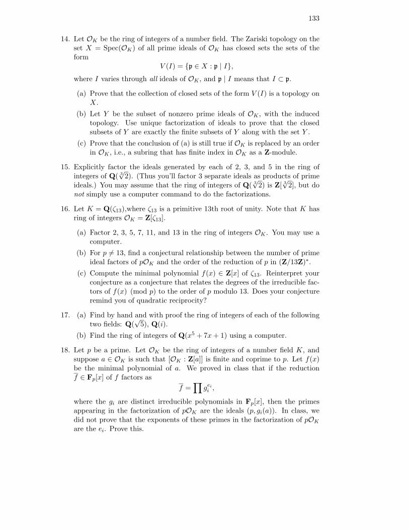
133

14. Let OK be the ring of integers of a number field. The Zariski topology on theset X = Spec(OK) of all prime ideals of OK has closed sets the sets of theform

V (I) = {p ∈ X : p | I},where I varies through all ideals of OK , and p | I means that I ⊂ p.

(a) Prove that the collection of closed sets of the form V (I) is a topology onX.

(b) Let Y be the subset of nonzero prime ideals of OK , with the inducedtopology. Use unique factorization of ideals to prove that the closedsubsets of Y are exactly the finite subsets of Y along with the set Y .

(c) Prove that the conclusion of (a) is still true if OK is replaced by an orderin OK , i.e., a subring that has finite index in OK as a Z-module.

15. Explicitly factor the ideals generated by each of 2, 3, and 5 in the ring ofintegers of Q( 3

√2). (Thus you’ll factor 3 separate ideals as products of prime

ideals.) You may assume that the ring of integers of Q( 3√

2) is Z[ 3√

2], but donot simply use a computer command to do the factorizations.

16. Let K = Q(ζ13),where ζ13 is a primitive 13th root of unity. Note that K hasring of integers OK = Z[ζ13].

(a) Factor 2, 3, 5, 7, 11, and 13 in the ring of integers OK . You may use acomputer.

(b) For p 6= 13, find a conjectural relationship between the number of primeideal factors of pOK and the order of the reduction of p in (Z/13Z)∗.

(c) Compute the minimal polynomial f(x) ∈ Z[x] of ζ13. Reinterpret yourconjecture as a conjecture that relates the degrees of the irreducible fac-tors of f(x) (mod p) to the order of p modulo 13. Does your conjectureremind you of quadratic reciprocity?

17. (a) Find by hand and with proof the ring of integers of each of the followingtwo fields: Q(

√5), Q(i).

(b) Find the ring of integers of Q(x5 + 7x + 1) using a computer.

18. Let p be a prime. Let OK be the ring of integers of a number field K, andsuppose a ∈ OK is such that [OK : Z[a]] is finite and coprime to p. Let f(x)be the minimal polynomial of a. We proved in class that if the reductionf ∈ Fp[x] of f factors as

f =∏

gei

i ,

where the gi are distinct irreducible polynomials in Fp[x], then the primesappearing in the factorization of pOK are the ideals (p, gi(a)). In class, wedid not prove that the exponents of these primes in the factorization of pOK

are the ei. Prove this.


19. Let a1 = 1 + i, a2 = 3 + 2i, and a3 = 3 + 4i as elements of Z[i].

(a) Prove that the ideals I1 = (a1), I2 = (a2), and I3 = (a3) are coprime inpairs.

(b) Compute #Z[i]/(I1I2I3).

(c) Find a single element in Z[i] that is congruent to n modulo In, for eachn ≤ 3.

20. Find an example of a field K of degree at least 4 such that the ring OK ofintegers of K is not of the form Z[a] for any a ∈ OK .

21. Let p be a prime ideal of OK , and suppose that OK/p is a finite field ofcharacteristic p ∈ Z. Prove that there is an element α ∈ OK such thatp = (p, α). This justifies why PARI can represent prime ideals of OK aspairs (p, α). (More generally, if I is an ideal of OK , we can choose one of theelements of I to be any nonzero element of I.)

22. (*) Give an example of an order O in the ring of integers of a number fieldand an ideal I such that I cannot be generated by 2 elements as an ideal.Does the Chinese Remainder Theorem hold in O? [The (*) means that thisproblem is more difficult than usual.]

23. For each of the following three fields, determining if there is an order of dis-criminant 20 contained in its ring of integers:

K = Q(√

5), K = Q(3√

2), and . . .

K any extension of Q of degree 2005. [Hint: for the last one, apply the exactform of our theorem about finiteness of class groups to the unit ideal to showthat the discriminant of a degree 2005 field must be large.]

24. Prove that the quantity Cr,s in our theorem about finiteness of the class groupcan be taken to be

(4π

)s n!nn , as follows (adapted from [SD01, pg. 19]): Let S

be the set of elements (x1, . . . , xn) ∈ Rn such that

|x1| + · · · |xr| + 2r+s∑

v=r+1

√x2

v + x2v+s ≤ 1.

(a) Prove that S is convex and that M = n−n, where

M = max{|x1 · · ·xr ·(x2r+1+x2

(r+1)+s) · · · (x2r+s+x2

n)| : (x1, . . . , xn) ∈ S}.

[Hint: For convexity, use the triangle inequality and that for 0 ≤ λ ≤ 1,we have

λ√

x21 + y2

1 + (1 − λ)√

x22 + y2

2

≥√

(λx1 + (1 − λ)x2)2 + (λy1 + (1 − λ)y2)2

135

for 0 ≤ λ ≤ 1. In polar coordinates this last inequality is

λr1 + (1 − λ)r2 ≥√

λ2r21 + 2λ(1 − λ)r1r2 cos(θ1 − θ2) + (1 − λ)2r2

2,

which is trivial. That M ≤ n−n follows from the inequality between thearithmetic and geometric means.

(b) Transforming pairs xv, xv+s from Cartesian to polar coordinates, showalso that v = 2r(2π)sDr,s(1), where

D`,m(t) =

∫· · ·

∫

R`,m(t)y1 · · · ymdx1 · · · dx`dy1 · · · dym

and R`,m(t) is given by xρ ≥ 0 (1 ≤ ρ ≤ `), yρ ≥ 0 (1 ≤ ρ ≤ m) and

x1 + · · · + x` + 2(y1 + · · · + ym) ≤ t.

(c) Prove that

D`,m(t) =

∫ t

0D`−1,m(t − x)dx =

∫ t/2

0D`,m−1(t − 2y)ydy

and deduce by induction that

D`,m(t) =4−mt`+2m

(` + 2m)!

25. Let K vary through all number fields. What torsion subgroups (UK)tor actu-ally occur?

26. If UK ≈ Zn × (UK)tor, we say that UK has rank n. Let K vary through allnumber fields. What ranks actually occur?

27. Let K vary through all number fields such that the group UK of units of K isa finite group. What finite groups UK actually occur?

28. Let K = Q(ζ5).

(a) Show that r = 0 and s = 2.

(b) Find explicit generators for the group of units of UK .

(c) Draw an illustration of the log map ϕ : UK → R2, including the hyper-plane x1+x2 = 0 and the lattice in the hyperplane spanned by the imageof UK .

29. Let K be a number field. Prove that p | dK if and only if p ramifies in K.(Note: This fact is proved in many books.)


30. Using Zorn’s lemma, one can show that there are homomorphisms Gal(Q/Q) →{±1} with finite image that are not continuous, since they do not factorthrough the Galois group of any finite Galois extension. [Hint: The extensionQ(

√d, d ∈ Q∗/(Q∗)2) is an extension of Q with Galois group X ≈ ∏

F2. Theindex-two open subgroups of X correspond to the quadratic extensions of Q.However, Zorn’s lemma implies that X contains many index-two subgroupsthat do not correspond to quadratic extensions of Q.]

31. (a) Give an example of a finite nontrivial Galois extension K of Q and aprime ideal p such that Dp = Gal(K/Q).

(b) Give an example of a finite nontrivial Galois extension K of Q and aprime ideal p such that Dp has order 1.

(c) Give an example of a finite Galois extension K of Q and a prime ideal p

such that Dp is not a normal subgroup of Gal(K/Q).

(d) Give an example of a finite Galois extension K of Q and a prime ideal p

such that Ip is not a normal subgroup of Gal(K/Q).

32. Let S3 by the symmetric group on three symbols, which has order 6.

(a) Observe that S3∼= D3, where D3 is the dihedral group of order 6, which

is the group of symmetries of an equilateral triangle.

(b) Use (32a) to write down an explicit embedding S3 ↪→ GL2(C).

(c) Let K be the number field Q( 3√

2, ω), where ω3 = 1 is a nontrivial cuberoot of unity. Show that K is a Galois extension with Galois groupisomorphic to S3.

(d) We thus obtain a 2-dimensional irreducible complex Galois representation

ρ : Gal(Q/Q) → Gal(K/Q) ∼= S3 ⊂ GL2(C).

Compute a representative matrix of Frobp and the characteristic polyno-mial of Frobp for p = 5, 7, 11, 13.

33. Look up the Riemann-Roch theorem in a book on algebraic curves.

(a) Write it down in your own words.

(b) Let E be an elliptic curve over a field K. Use the Riemann-Roch theoremto deduce that the natural map

E(K) → Pic0(E/K)

is an isomorphism.

34. Suppose G is a finite group and A is a finite G-module. Prove that for any q,the group Hq(G, A) is a torsion abelian group of exponent dividing the order#A of A.

137

35. Let K = Q(√

5) and let A = UK be the group of units of K, which is a moduleover the group G = Gal(K/Q). Compute the cohomology groups H0(G, A)and H1(G, A). (You shouldn’t use a computer, except maybe to determineUK .)

36. Let K = Q(√−23) and let C be the class group of Q(

√−23), which is a

module over the Galois group G = Gal(K/Q). Determine H0(G, C) andH1(G, C).

37. Let E be the elliptic curve y2 = x3 + x + 1. Let E[2] be the group of pointsof order dividing 2 on E. Let

ρE,2 : Gal(Q/Q) → Aut(E[2])

be the mod 2 Galois representation associated to E.

(a) Find the fixed field K of ker(ρE,2).

(b) Is ρE,2 surjective?

(c) Find the group Gal(K/Q).

(d) Which primes are ramified in K?

(e) Let I be an inertia group above 2, which is one of the ramified primes.Determine E[2]I explicitly for your choice of I. What is the characteristicpolynomial of Frob2 acting on E[2]I .

(f) What is the characteristic polynomial of Frob3 acting on E[2]?

(g) Let K be a number field. Prove that there is a finite set S of primes of Ksuch that

OK,S = {a ∈ K∗ : ordp(aOK) ≥ 0 all p 6∈ S} ∪ {0}

is a prinicipal ideal domain. The condition ordp(aOK) ≥ 0 means that inthe prime ideal factorization of the fractional ideal aOK , we have that p

occurs to a nonnegative power.

(h) Let a ∈ K and n a positive integer. Prove that L = K(a1/n) is unramifiedoutside the primes that divide n and the norm of a. This means that if p

is a prime of OK , and p is coprime to n NormL/K(a)OK , then the primefactorization of pOL involves no primes with exponent bigger than 1.

(i) Write down a proof of Hilbert’s Theorem 90, formulated as the statementthat for any number field K, we have

H1(K, K∗) = 0.

Bibliography

[ABC+] B. Allombert, K. Belabas, H. Cohen, X. Roblot, and I. Zakhare-vitch, PARI/GP, http://pari.math.u-bordeaux.fr/.

[Art23] E. Artin, Uber eine neue Art von L-reihen, Abh. Math. Sem.Univ. Hamburg 3 (1923), 89–108.

[Art30] E Artin, Zur Theorie der L-Reihen mit allgemeinen Gruppen-charakteren, Abh. math. Semin. Univ. Hamburg 8 (1930), 292–306.

[Art91] M. Artin, Algebra, Prentice Hall Inc., Englewood Cliffs, NJ, 1991.MR 92g:00001

[BCP97] W. Bosma, J. Cannon, and C. Playoust, The Magma algebra sys-tem. I. The user language, J. Symbolic Comput. 24 (1997), no. 3–4, 235–265, Computational algebra and number theory (London,1993). MR 1 484 478

[BDSBT01] Kevin Buzzard, Mark Dickinson, Nick Shepherd-Barron, andRichard Taylor, On icosahedral Artin representations, DukeMath. J. 109 (2001), no. 2, 283–318. MR MR1845181(2002k:11078)

[BL94] J. A. Buchmann and H. W. Lenstra, Jr., Approximating rings ofintegers in number fields, J. Theor. Nombres Bordeaux 6 (1994),no. 2, 221–260. MR MR1360644 (96m:11092)

[BS02] K. Buzzard and W.A. Stein, A mod five approach to modularity oficosahedral Galois representations, Pacific J. Math. 203 (2002),no. 2, 265–282. MR 2003c:11052

[Buh78] J. P. Buhler, Icosahedral Galois representations, Springer-Verlag,Berlin, 1978, Lecture Notes in Mathematics, Vol. 654.

[Cas67] J. W. S. Cassels, Global fields, Algebraic Number Theory (Proc.Instructional Conf., Brighton, 1965), Thompson, Washington,D.C., 1967, pp. 42–84.

[CL84] H. Cohen and H. W. Lenstra, Jr., Heuristics on class groupsof number fields, Number theory, Noordwijkerhout 1983 (Noord-wijkerhout, 1983), Lecture Notes in Math., vol. 1068, Springer,Berlin, 1984, pp. 33–62. MR MR756082 (85j:11144)

139

140 BIBLIOGRAPHY

[Coh93] H. Cohen, A course in computational algebraic number theory,Springer-Verlag, Berlin, 1993. MR 94i:11105

[Cp86] J. W. S. Cassels and A. Frohlich (eds.), Algebraic number theory,London, Academic Press Inc. [Harcourt Brace Jovanovich Pub-lishers], 1986, Reprint of the 1967 original.

[EH00] D. Eisenbud and J. Harris, The geometry of schemes, Springer-Verlag, New York, 2000. MR 2001d:14002

[Fre94] G. Frey (ed.), On Artin’s conjecture for odd 2-dimensional repre-sentations, Springer-Verlag, Berlin, 1994, 1585. MR 95i:11001

[Har77] R. Hartshorne, Algebraic Geometry, Springer-Verlag, New York,1977, Graduate Texts in Mathematics, No. 52.

[Lan80] R. P. Langlands, Base change for GL(2), Princeton UniversityPress, Princeton, N.J., 1980.

[Len02] H. W. Lenstra, Jr., Solving the Pell equation, Notices Amer.Math. Soc. 49 (2002), no. 2, 182–192. MR 2002i:11028

[LL93] A. K. Lenstra and H. W. Lenstra, Jr. (eds.), The developmentof the number field sieve, Springer-Verlag, Berlin, 1993. MR96m:11116

[SD01] H. P. F. Swinnerton-Dyer, A brief guide to algebraic number the-ory, London Mathematical Society Student Texts, vol. 50, Cam-bridge University Press, Cambridge, 2001. MR 2002a:11117

[Ser79] J-P. Serre, Local fields, Springer-Verlag, New York, 1979, Trans-lated from the French by Marvin Jay Greenberg.

[Sil92] J. H. Silverman, The arithmetic of elliptic curves, Springer-Verlag, New York, 1992, Corrected reprint of the 1986 original.

[Ste] W.A. Stein, Elementary Number Theory,http://modular.fas.harvard.edu/ent/.

introduction to algebraic number theory - william a. stein · 10 chapter 1. introduction 1.2 what...

Documents