introduction to analysis - reed collegepeople.reed.edu/~iswanson/analysisconstructr.pdfpreface these...
TRANSCRIPT

Introduction to Analysis
Irena Swanson
Reed College
Fall 2020

Table of contents
Preface 7
The briefest overview, motivation, notation 9
Chapter 1: How we will do mathematics 13
Section 1.1: Statements and proof methods 13
Section 1.2: Statements with quantifiers 25
Section 1.3: More proof methods, and negation 28
Section 1.4: Summation 34
Section 1.5: Proofs by (mathematical) induction 36
Section 1.6: Pascal’s triangle 45
Chapter 2: Concepts with which we will do mathematics 49
Section 2.1: Sets 49
Section 2.2: Cartesian product 58
Section 2.3: Relations, equivalence relations 59
Section 2.4: Functions 65
Section 2.5: Binary operations 75
Section 2.6: Fields 82
Section 2.7: Order on sets, ordered fields 86
Section 2.8: What are the integers and the rational numbers? 92
Section 2.9: Increasing and decreasing functions 94
Section 2.10: Absolute values 97
Chapter 3: Construction of the basic number systems 100
Section 3.1: Inductive sets and a construction of natural numbers 100
Section 3.2: Arithmetic on N0 105
Section 3.3: Order on N0 108
Section 3.4: Cancellation in N0 111
Section 3.5: Construction of Z, arithmetic, and order on Z 112
Section 3.6: Construction of the ordered field Q of rational numbers 118
4
Section 3.7: Construction of the field R of real numbers 122
Section 3.8: Order on R, the least upper/greatest lower bound theorem 131
Section 3.9: Complex numbers 133
Section 3.10: Functions related to complex numbers 136
Section 3.11: Absolute value in C 138
Section 3.12: Polar coordinates 141
Section 3.13: Topology on the fields of real and complex numbers 147
Section 3.14: The Heine-Borel theorem 150
Chapter 4: Limits of functions 154
Section 4.1: Limit of a function 154
Section 4.2: When a number is not a limit 165
Section 4.3: Limit theorems 168
Section 4.4: Infinite limits (for real-valued functions) 176
Section 4.5: Limits at infinity 180
Chapter 5: Continuity 182
Section 5.1: Continuous functions 182
Section 5.2: Topology and the Extreme value theorem 187
Section 5.3: Intermediate value theorem 190
Section 5.4: Radical functions 194
Section 5.5: Uniform continuity 198
Chapter 6: Differentiation 202
Section 6.1: Definition of derivatives 202
Section 6.2: Basic properties of derivatives 206
Section 6.3: The Mean value theorem 214
Section 6.4: L’Hopital’s rule 219
Section 6.5: Higher-order derivatives, Taylor polynomials 222
Chapter 7: Integration 227
Section 7.1: Approximating areas 227
Section 7.2: Computing integrals from upper and lower sums 237
Section 7.3: What functions are integrable? 240
Section 7.4: The Fundamental theorem of calculus 245
Section 7.5: Integration of complex-valued functions 252
Section 7.6: Natural logarithm and the exponential functions 253
Section 7.7: Applications of integration 258
Chapter 8: Sequences 265
5
Section 8.1: Introduction to sequences 265
Section 8.2: Convergence of infinite sequences 270
Section 8.3: Divergence of infinite sequences and infinite limits 277
Section 8.4: Convergence theorems via epsilon-N proofs 281
Section 8.5: Convergence theorems via functions 287
Section 8.6: Bounded sequences, monotone sequences, ratio test 290
Section 8.7: Cauchy sequences, completeness of R, C 294
Section 8.8: Subsequences 298
Section 8.9: Liminf, limsup for real-valued sequences 300
Chapter 9: Infinite series and power series 306
Section 9.1: Infinite series 306
Section 9.2: Convergence and divergence theorems for series 310
Section 9.3: Power series 317
Section 9.4: Differentiation of power series 322
Section 9.5: Numerical evaluations of some series 325
Section 9.6: Some technical aspects of power series 327
Section 9.7: Taylor series 331
Section 9.8: A special function 334
Section 9.9: A special function, continued 336
Section 9.10: Trigonometry 343
Section 9.11: Examples of L’Hopital’s rule 346
Section 9.12: Further specialized uses of trigonometry 347
Appendix A: Advice on writing mathematics 353
Appendix B: What you should never forget 357
Index 361


Preface
These notes were written expressly for Mathematics 112 at Reed College, with first
usage in the spring of 2013. The title of the course is “Introduction to Analysis”. The
prerequisite is calculus. Recently used textbooks have been Steven R. Lay’s “Analysis,
With an Introduction to Proof ” (Prentice Hall, Inc., Englewood Cliffs, NJ, 1986, 4th
edition), and Ray Mayer’s in-house notes “Introduction to Analysis” (2006, available at
http://www.reed.edu/~mayer/math112.html/index.html).
In Math 112, students learn to write proofs while at the same time learning about bi-
nary operations, orders, fields, ordered fields, complete fields, complex numbers, sequences,
and series. We also review limits, continuity, differentiation, and integration. My aim for
these notes is to constitute a self-contained book that covers the standard topics of a course
in introductory analysis, that handles complex-valued functions, sequences, and series, that
has enough examples and exercises, that is rigorous, and is accessible to Reed College un-
dergraduates. I currently maintain two versions of these notes, one in which the natural,
rational and real numbers are constructed and the Least upper bound theorem is proved
for the ordered field of real numbers, and one version in which the Least upper bound
property is assumed for the ordered field of real numbers. You are currently reading the
longer, former version. See my Math 112 webpage www.reed.edu/~iswanson/112.html
for links to both versions.
Chapter 1 is about how we do mathematics: basic logic, proof methods, and Pascal’s
triangle for practicing proofs. Chapter 2 introduces foundational concepts: sets, Carte-
sian products, relations, functions, binary operations, fields, ordered fields, Archimedean
property for the set of real numbers. In Chapters 1 and 2 we assume knowledge of high
school mathematics so that we do not practice abstract concepts and methods in a vac-
uum. Chapter 3 through Section 3.8 takes a step back: we “forget” most previously learned
mathematics, and we use the newly learned abstract tools to construct natural numbers,
integers, rational numbers, real numbers, with all the arithmetic and order. I do not teach
these constructions in great detail; my aim is to give a sense of them and to practice abstract
logical thinking. The remaining sections in Chapter 3 are new material for most students:
the field of complex numbers, and some topology. I cover the last section of Chapter 3 very
lightly. Subsequent chapters cover standard material for introduction to analysis: limits,
continuity, differentiation, integration, sequences, series, ending with the development of
the power series∑∞k=0
xk
k! , the exponential and the trigonometric functions. Since students
have seen limits, continuity, differentiation and integration before, I go through chapters 4
through 7 quickly. I slow down for sequences and series (chapters 8 and 9).
An effort is made throughout to use only what had been proved. When trigonometric
functions appear in earlier exercises they are accompanied with a careful listing of the
8 Preface
needed assumptions about them. For this reason, the chapters on differentiation and
integration do not have the usual palette of examples of other books. The final sections of
the last chapter make up for it and work out much trigonometry in great detail and depth.
I acknowledge and thank the support from the Dean of Faculty of Reed College
to fund exercise and proofreading support in the summer of 2012 for Maddie Brandt,
Munyo Frey-Edwards, and Kelsey Houston-Edwards. I also thank the following people
for their valuable feedback: Mark Angeles, Josie Baker, Marcus Bamberger, Anji Bodony,
Zachary Campbell, Nick Chaiyachakorn, Safia Chettih, Laura Dallago, Andrew Erlanger,
Joel Franklin, Darij Grinberg, Rohr Hautala, Palak Jain, Ya Jiang, Albyn Jones, Wil-
low Kelleigh, Mason Kennedy, Christopher Keane, Michael Keppler, Ryan Kobler, Oleks
Lushchyk, Molly Maguire, Benjamin Morrison, Samuel Olson, Kyle Ormsby, Angelica Os-
orno, Shannon Pearson, David Perkinson, Jeremy Rachels, Ezra Schwartz, Jacob Sharkan-
sky, Marika Swanberg, Simon Swanson, Matyas Szabo, Ruth Valsquier, Xingyi Wang,
Emerson Webb, Livia Xu, Qiaoyu Yang, Dean Young, Eric Zhang, and Jialun Zhao. If you
have further comments or corrections, please send them to [email protected].

The briefest overview, motivation, notation
What are the meanings of the following:
5 + 6
7 · 98− 4
4/5√
2
4− 8
1/3 = 0.333 . . . 1 = 3 · 1/3 = 0.999 . . .
(a · b)2 = a2 · b2
(a+ b) · (c+ d) = ac+ ad+ bc+ bd
(a+ b) · (a− b) = a2 − b2
(a+ b)2 = a2 + 2ab+ b2
√a ·√b =√ab (for which a, b?)
What is going on:√−4 ·√−9 =
√(−4)(−9) =
√36 = 6,
√−4 ·√−9 = 2i · 3i = −6
You know all of the above except possibly the complex numbers in the last two rows,
where obviously something went wrong. We will not resolve this last issue until later in
the semester, but the point for now is that we do need to reason carefully.
The main goal of this class is to learn to reason carefully, rigorously. Since one
cannot reason in a vacuum, we will (but of course) be learning a lot of mathematics as
well: sets, logic, various number systems, fields, the field of real numbers, the field of
complex numbers, sequences, series, some calculus, and that eix = cosx+ i sinx.
We will make it all rigorous, i.e., we will be doing proofs. A proof is a sequence of
steps that logically follow from previously accepted knowledge.
But no matter what you do, never divide by 0. For further wise advice, turn to
Appendix A.
[Notational convention: Text between square brackets in this font and in
red color should be read as a possible reasoning going on in the background
in your head, and not as part of formal writing.]
†1. Exercises with a dagger are invoked later in the text.
*2. Exercises with a star are more difficult.

Introduction to Analysis

Chapter 1: How we will do mathematics
1.1 Statements and proof methods
Definition 1.1.1. A statement is a reasonably grammatical and unambiguous sentence
that can be declared either true or false.
Why do we specify “reasonably grammatical”? We do not disqualify a statement just
because of poor grammar, nevertheless, we strive to use correct grammar and to express the
meaning clearly. And what do we mean by true or false? For our purposes, a statement
is false if there is at least one counterexample to it, and a statement is true if it has been
proved so, or if we assume it to be true.
Examples and non-examples 1.1.2.
(i) The sum of 1 and 2 equals 3. (This is a statement; it is always true.)
(ii) Seventeen. (This is not a statement.)
(iii) Seventeen is the seventh prime number. (This is a true statement.)
(iv) Is x positive? (This is not a statement.)
(v) 1 = 2.* (This is a false statement.)
(vi) For every real number ε > 0 there exists a real number δ > 0 such that for all x,
if 0 < |x − a| < δ then x is in the domain of f and |f(x) − L| < ε. (This is a
statement, and it is (a part of) the definition of the limit of a (special) function f
at a being L. Out of context, this statement is neither true or false, but we can
prove it or assume it for various functions f .) )
(vii) Every even number greater than 4 can be written as a sum of two odd primes.
(This statement is known as Goldbach’s conjecture. No counterexample is
known, and no proof has been devised, so it is currently not known if it is true or
false.)
These examples show that not all statements have a definitive truth value. What
makes them statements is that after possibly arbitrarily assigning them truth values, differ-
ent consequences follow. For example, if we assume that (vi) above is true, then the graph
of f near a is close to the graph of the constant function L. If instead we assume that
(vi) above is false, then the graph of f near a has infinitely many values at some vertical
distance away from L no matter how much we zoom in at a. With this in mind, even “I
am good” is a statement: if I am good, then I get a cookie, but if I am not good, then you
* This statement can also be written in plain English as “One equals two.” In mathematics it is acceptable
to use symbolic notation to some extent, but keep in mind that too many symbols can make a sentence hard to
read. In general we avoid starting sentences with a symbol. In particular, do not make the following sentence.
“=” is a verb. Instead make a sentence such as the following one. Note that “=” is a verb.
14 Chapter 1: How we will do mathematics
get the cookie. On the other hand, if “Hello” were to be true or false, I would not be able
to make any further deductions about the world or my next action, so that “Hello” is not
a statement, but only a sentence.
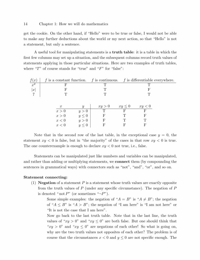
A useful tool for manipulating statements is a truth table: it is a table in which the
first few columns may set up a situation, and the subsequent columns record truth values of
statements applying in those particular situations. Here are two examples of truth tables,
where “T” of course stands for “true” and “F” for “false”:
f(x) f is a constant function. f is continuous. f is differentiable everywhere.x2 F T T|x| F T F7 T T T
x y xy > 0 xy ≤ 0 xy < 0x > 0 y > 0 T F Fx > 0 y ≤ 0 F T Fx < 0 y > 0 F T Tx < 0 y ≤ 0 F F F
Note that in the second row of the last table, in the exceptional case y = 0, the
statement xy < 0 is false, but in “the majority” of the cases in that row xy < 0 is true.
The one counterexample is enough to declare xy < 0 not true, i.e., false.
Statements can be manipulated just like numbers and variables can be manipulated,
and rather than adding or multiplying statements, we connect them (by compounding the
sentences in grammatical ways) with connectors such as “not”, “and”, “or”, and so on.
Statement connecting:
(1) Negation of a statement P is a statement whose truth values are exactly opposite
from the truth values of P (under any specific circumstance). The negation of P
is denoted “ notP” (or sometimes “¬P”).
Some simple examples: the negation of “A = B” is “A 6= B”; the negation
of “A ≤ B” is “A > B”; the negation of “I am here” is “I am not here” or
“It is not the case that I am here”.
Now go back to the last truth table. Note that in the last line, the truth
values of “xy > 0” and “xy ≤ 0” are both false. But one should think that
“xy > 0” and “xy ≤ 0” are negations of each other! So what is going on,
why are the two truth values not opposites of each other? The problem is of
course that the circumstances x < 0 and y ≤ 0 are not specific enough. The
Section 1.1: Statements and proof methods 15
statement “xy > 0” is under these circumstances false precisely when y = 0,
but then “xy ≤ 0” is true. Similarly, the statement “xy ≤ 0” is under the
given circumstances false precisely when y < 0, but then “xy > 0” is true.
Thus, once we make the conditions specific enough, then the truth values of
“xy > 0” and “xy ≤ 0” are opposite, so that the two statements are indeed
negations of each other.
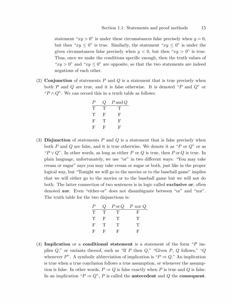
(2) Conjunction of statements P and Q is a statement that is true precisely when
both P and Q are true, and it is false otherwise. It is denoted “P and Q” or
“P ∧Q”. We can record this in a truth table as follows:
P Q P andQ
T T T
T F F
F T F
F F F
(3) Disjunction of statements P and Q is a statement that is false precisely when
both P and Q are false, and it is true otherwise. We denote it as “P or Q” or as
“P ∨Q”. In other words, as long as either P or Q is true, then P orQ is true. In
plain language, unfortunately, we use “or” in two different ways: “You may take
cream or sugar” says you may take cream or sugar or both, just like in the proper
logical way, but “Tonight we will go to the movies or to the baseball game” implies
that we will either go to the movies or to the baseball game but we will not do
both. The latter connection of two sentences is in logic called exclusive or, often
denoted xor. Even “either-or” does not disambiguate between “or” and “xor”.
The truth table for the two disjunctions is:
P Q P orQ P xor Q
T T T F
T F T T
F T T T
F F F F
(4) Implication or a conditional statement is a statement of the form “P im-
plies Q,” or variants thereof, such as “If P then Q,” “Given P , Q follows,” “Q
whenever P”. A symbolic abbreviation of implication is “P ⇒ Q.” An implication
is true when a true conclusion follows a true assumption, or whenever the assump-
tion is false. In other words, P ⇒ Q is false exactly when P is true and Q is false.
In an implication “P ⇒ Q”, P is called the antecedent and Q the consequent.
16 Chapter 1: How we will do mathematics
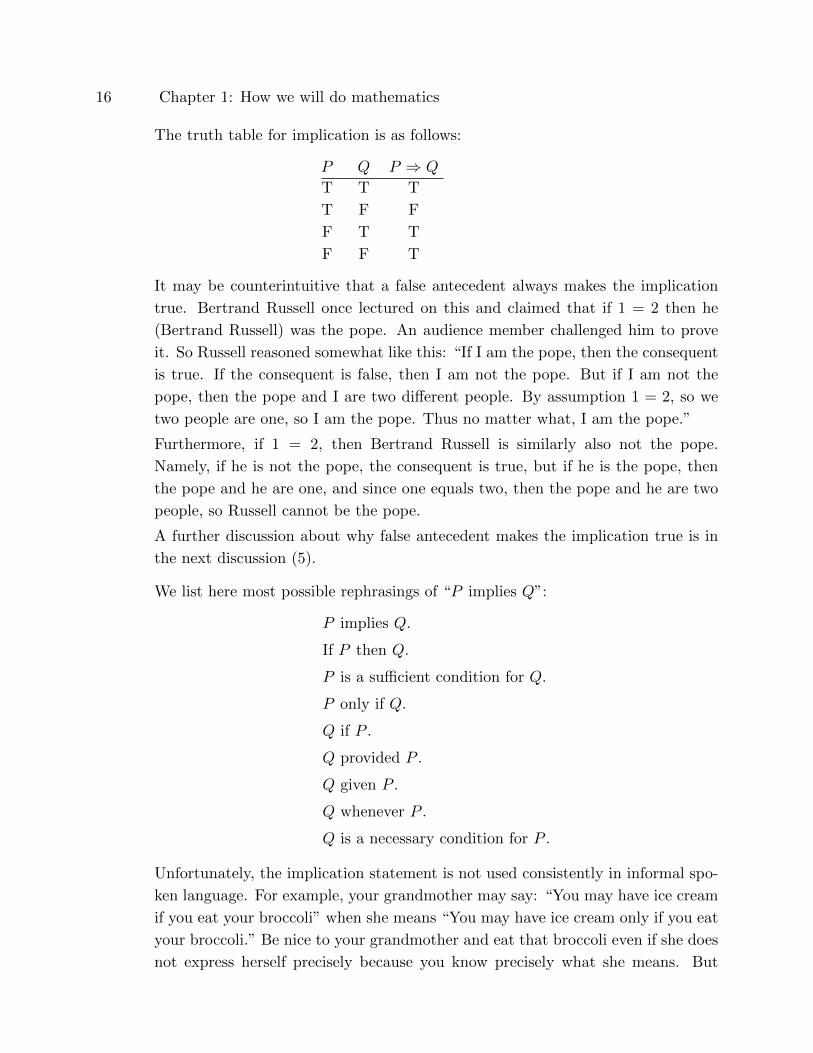
The truth table for implication is as follows:
P Q P ⇒ Q
T T T
T F F
F T T
F F T
It may be counterintuitive that a false antecedent always makes the implication
true. Bertrand Russell once lectured on this and claimed that if 1 = 2 then he
(Bertrand Russell) was the pope. An audience member challenged him to prove
it. So Russell reasoned somewhat like this: “If I am the pope, then the consequent
is true. If the consequent is false, then I am not the pope. But if I am not the
pope, then the pope and I are two different people. By assumption 1 = 2, so we
two people are one, so I am the pope. Thus no matter what, I am the pope.”
Furthermore, if 1 = 2, then Bertrand Russell is similarly also not the pope.
Namely, if he is not the pope, the consequent is true, but if he is the pope, then
the pope and he are one, and since one equals two, then the pope and he are two
people, so Russell cannot be the pope.
A further discussion about why false antecedent makes the implication true is in
the next discussion (5).
We list here most possible rephrasings of “P implies Q”:
P implies Q.
If P then Q.
P is a sufficient condition for Q.
P only if Q.
Q if P .
Q provided P .
Q given P .
Q whenever P .
Q is a necessary condition for P .
Unfortunately, the implication statement is not used consistently in informal spo-
ken language. For example, your grandmother may say: “You may have ice cream
if you eat your broccoli” when she means “You may have ice cream only if you eat
your broccoli.” Be nice to your grandmother and eat that broccoli even if she does
not express herself precisely because you know precisely what she means. But
Section 1.1: Statements and proof methods 17
in mathematics you do have to express yourself precisely! (Well, read the next
paragraph.)
Even in mathematics some shortcuts in precise expressions are acceptable. Here
is an example. The statements “An object x has property P if somethingorother
holds” and “An object x has property P if and only if somethingorother holds” (see
(5) below for “if and only if”) in general have different truth values and the proof
of the second is longer. However, the definition of what it means for an object
to have property P in terms of somethingorother is usually phrased with “if”, but
“if and only if” is meant. For example, the following is standard: “Definition:
A positive integer strictly bigger than 1 is prime if whenever it can be written as
a product of two positive integers, one of the two factors must be 1.” The given
definition, if read logically precisely, since it said nothing about numbers such as
4 = 2 · 2, would allow us to call 4 prime. However, it is an understood shortcut
that only the numbers with the stated property are called prime.
(5) Equivalence or the logical biconditional of P and Q stands for the compound
statement (P ⇒ Q) and (Q⇒ P ). It is abbreviated “P ⇔ Q” or “P iff Q”, and is
true precisely when P and Q have the same truth values.
For example, for real numbers x and y, the statement “x ≤ y+1” is equivalent
to “x − 1 ≤ y.” Another example: “2x = 4x2” is equivalent to “x = 2x2,”
but it is not equivalent to “1 = 2x.” (Say why!)
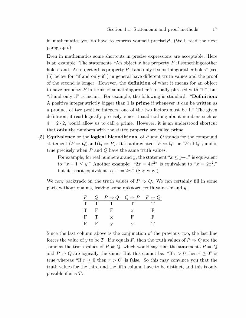
We now backtrack on the truth values of P ⇒ Q. We can certainly fill in some
parts without qualms, leaving some unknown truth values x and y:
P Q P ⇒ Q Q⇒ P P ⇔ Q
T T T T T
T F F x F
F T x F F
F F y y T
Since the last column above is the conjunction of the previous two, the last line
forces the value of y to be T . If x equals F , then the truth values of P ⇒ Q are the
same as the truth values of P ⇔ Q, which would say that the statements P ⇒ Q
and P ⇔ Q are logically the same. But this cannot be: “If r > 0 then r ≥ 0” is
true whereas “If r ≥ 0 then r > 0” is false. So this may convince you that the
truth values for the third and the fifth column have to be distinct, and this is only
possible if x is T .

18 Chapter 1: How we will do mathematics
Here is the truth table for all the connectives so far:
P Q notP P andQ P orQ P xor Q P ⇒ Q P ⇔ Q
T T F T T F T T
T F F F T T F F
F T T F T T T F
F F T F F F T T
One can form more elaborate truth tables if we start not with two statements P
and Q but with three or more. Examples of logically compounding P,Q, and R
are: P andQ andR, (P andQ)⇒ Q, et cetera. For manipulating three statements,
we would fill a total of 8 rows of truth values, for four statements there would be
16 rows, and so on.
(6) Proof of P is a series of steps (in statement form) that establish beyond doubt that
P is true under all circumstances, weather conditions, political regimes, time of
day... The logical reasoning that goes into mathematical proofs is called deductive
reasoning. Whereas both guessing and intuition can help you find the next step
in your mathematical proof, only the logical parts are trusted and get written
down. Proofs are a mathematician’s most important tool; the book contains many
examples, and the next few pages give some examples and ideas of what proofs
are.
Ends of proofs are usually marked by , , //, or QED (for “quod erat demon-
strandum”, which is Latin for “that which was to be proved”). It is a good idea to
mark the completions of proofs especially when they are long or with many parts
and steps — that helps the readers know that nothing else is to be added.
The most trivial proofs simply invoke a definition or axiom, such as “An even
integer is of the form 2 times an integer,” “An odd integer is of the form 1 plus 2
times an integer,” or, “A positive integer is prime if whenever it can be written
as a product of two positive integers, one of the two factors is 1.”
Another type of proof consists of filling in a truth table. For example, P or ( notP )
is always true, no matter what the truth value of P is, and this can be easily verified
with the truth table:
P notP P or notP
T F T
F T T
A formula using logical statements that is always true is called a tautology.
So P or notP is a tautology. Here is another example of tautology: ((P ⇒
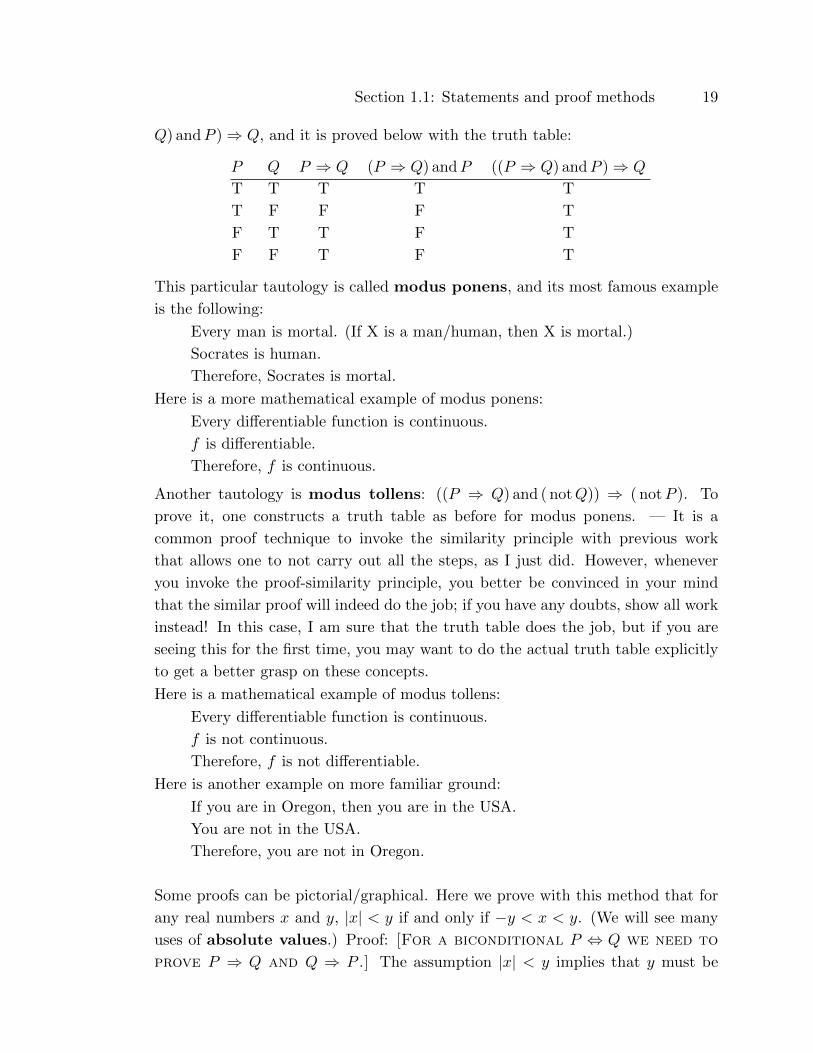
Section 1.1: Statements and proof methods 19
Q) andP )⇒ Q, and it is proved below with the truth table:
P Q P ⇒ Q (P ⇒ Q) andP ((P ⇒ Q) andP )⇒ Q
T T T T T
T F F F T
F T T F T
F F T F T
This particular tautology is called modus ponens, and its most famous example
is the following:
Every man is mortal. (If X is a man/human, then X is mortal.)
Socrates is human.
Therefore, Socrates is mortal.
Here is a more mathematical example of modus ponens:
Every differentiable function is continuous.
f is differentiable.
Therefore, f is continuous.
Another tautology is modus tollens: ((P ⇒ Q) and ( notQ)) ⇒ ( notP ). To
prove it, one constructs a truth table as before for modus ponens. — It is a
common proof technique to invoke the similarity principle with previous work
that allows one to not carry out all the steps, as I just did. However, whenever
you invoke the proof-similarity principle, you better be convinced in your mind
that the similar proof will indeed do the job; if you have any doubts, show all work
instead! In this case, I am sure that the truth table does the job, but if you are
seeing this for the first time, you may want to do the actual truth table explicitly
to get a better grasp on these concepts.
Here is a mathematical example of modus tollens:
Every differentiable function is continuous.
f is not continuous.
Therefore, f is not differentiable.
Here is another example on more familiar ground:
If you are in Oregon, then you are in the USA.
You are not in the USA.
Therefore, you are not in Oregon.
Some proofs can be pictorial/graphical. Here we prove with this method that for
any real numbers x and y, |x| < y if and only if −y < x < y. (We will see many
uses of absolute values.) Proof: [For a biconditional P ⇔ Q we need to
prove P ⇒ Q and Q ⇒ P .] The assumption |x| < y implies that y must be
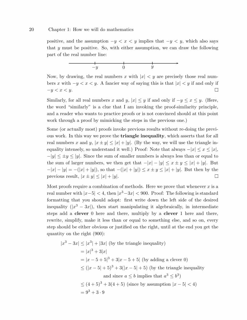
20 Chapter 1: How we will do mathematics
positive, and the assumption −y < x < y implies that −y < y, which also says
that y must be positive. So, with either assumption, we can draw the following
part of the real number line:
−y y0
Now, by drawing, the real numbers x with |x| < y are precisely those real num-
bers x with −y < x < y. A fancier way of saying this is that |x| < y if and only if
−y < x < y.
Similarly, for all real numbers x and y, |x| ≤ y if and only if −y ≤ x ≤ y. (Here,
the word “similarly” is a clue that I am invoking the proof-similarity principle,
and a reader who wants to practice proofs or is not convinced should at this point
work through a proof by mimicking the steps in the previous one.)
Some (or actually most) proofs invoke previous results without re-doing the previ-
ous work. In this way we prove the triangle inequality, which asserts that for all
real numbers x and y, |x± y| ≤ |x|+ |y|. (By the way, we will use the triangle in-
equality intensely, so understand it well.) Proof: Note that always −|x| ≤ x ≤ |x|,−|y| ≤ ±y ≤ |y|. Since the sum of smaller numbers is always less than or equal to
the sum of larger numbers, we then get that −|x| − |y| ≤ x ± y ≤ |x| + |y|. But
−|x| − |y| = −(|x|+ |y|), so that −(|x|+ |y|) ≤ x± y ≤ |x|+ |y|. But then by the
previous result, |x± y| ≤ |x|+ |y|.
Most proofs require a combination of methods. Here we prove that whenever x is a
real number with |x−5| < 4, then |x3−3x| < 900. Proof: The following is standard
formatting that you should adopt: first write down the left side of the desired
inequality (|x3 − 3x|), then start manipulating it algebraically, in intermediate
steps add a clever 0 here and there, multiply by a clever 1 here and there,
rewrite, simplify, make it less than or equal to something else, and so on, every
step should be either obvious or justified on the right, until at the end you get the
quantity on the right (900):
|x3 − 3x| ≤ |x3|+ |3x| (by the triangle inequality)
= |x|3 + 3|x|= |x− 5 + 5|3 + 3|x− 5 + 5| (by adding a clever 0)
≤ (|x− 5|+ 5)3 + 3(|x− 5|+ 5) (by the triangle inequality
and since a ≤ b implies that a3 ≤ b3)
≤ (4 + 5)3 + 3(4 + 5) (since by assumption |x− 5| < 4)
= 93 + 3 · 9
Section 1.1: Statements and proof methods 21
= 9(92 + 3)
< 900.
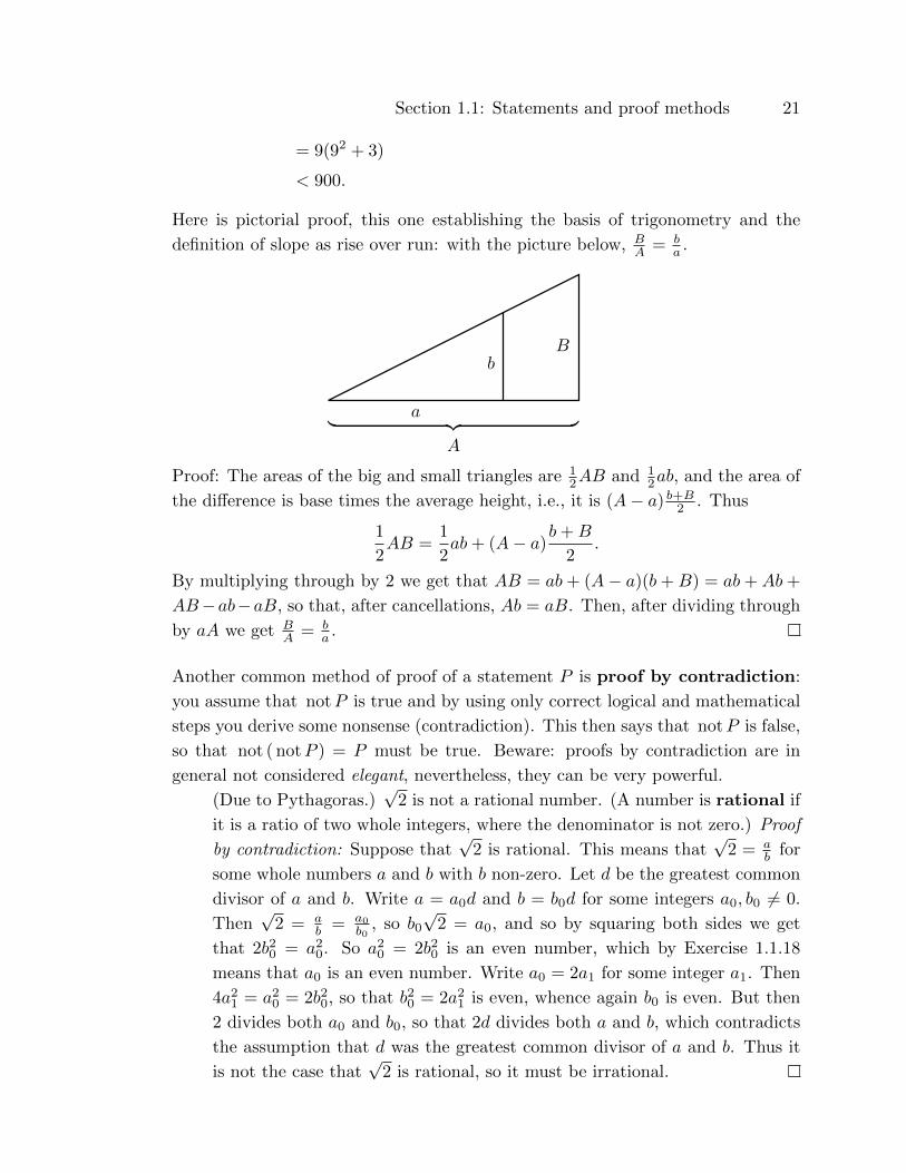
Here is pictorial proof, this one establishing the basis of trigonometry and the
definition of slope as rise over run: with the picture below, BA = b
a .
a︸ ︷︷ ︸
A
bB
Proof: The areas of the big and small triangles are 12AB and 1
2ab, and the area of
the difference is base times the average height, i.e., it is (A− a) b+B2 . Thus
1
2AB =
1
2ab+ (A− a)
b+B
2.
By multiplying through by 2 we get that AB = ab+ (A− a)(b+B) = ab+ Ab+
AB−ab−aB, so that, after cancellations, Ab = aB. Then, after dividing through
by aA we get BA = b
a .
Another common method of proof of a statement P is proof by contradiction:
you assume that notP is true and by using only correct logical and mathematical
steps you derive some nonsense (contradiction). This then says that notP is false,
so that not ( notP ) = P must be true. Beware: proofs by contradiction are in
general not considered elegant, nevertheless, they can be very powerful.
(Due to Pythagoras.)√
2 is not a rational number. (A number is rational if
it is a ratio of two whole integers, where the denominator is not zero.) Proof
by contradiction: Suppose that√
2 is rational. This means that√
2 = ab for
some whole numbers a and b with b non-zero. Let d be the greatest common
divisor of a and b. Write a = a0d and b = b0d for some integers a0, b0 6= 0.
Then√
2 = ab = a0
b0, so b0
√2 = a0, and so by squaring both sides we get
that 2b20 = a20. So a2
0 = 2b20 is an even number, which by Exercise 1.1.18
means that a0 is an even number. Write a0 = 2a1 for some integer a1. Then
4a21 = a2
0 = 2b20, so that b20 = 2a21 is even, whence again b0 is even. But then
2 divides both a0 and b0, so that 2d divides both a and b, which contradicts
the assumption that d was the greatest common divisor of a and b. Thus it
is not the case that√
2 is rational, so it must be irrational.

22 Chapter 1: How we will do mathematics
Exercises for Section 1.1
1.1.1. Determine whether the following statements are true or false, and justify:
i) 3 is odd or 5 is even.
ii) If n is even, then 3n is prime.
iii) If 3n is even, then n is prime.
iv) If n is prime, then 3n is odd.
v) If 3n is prime, then n is odd.
vi) (P andQ)⇒ P .
1.1.2. Sometimes statements are not written precisely enough. For example, “It is not the
case that 3 is prime and 5 is even” may be saying “ not (3 is prime and 5 is even),” or it
may be saying “( not (3 is prime)) and (5 is even).” The first option is true and the second
is false.
Similarly analyze several possible interpretations of the following ambiguous sentences:
i) If 6 is prime then 7 is even or 5 is odd.
ii) It is not the case that 3 is prime or if 6 is prime then 7 is even or 5 is odd.
General advice: Write precisely; aim to not be misunderstood.
1.1.3. Suppose that P ⇒ Q is true and that Q is false. Prove that P is false.
1.1.4. Prove that P ⇒ Q is equivalent to ( notQ)⇒ ( notP ).
1.1.5. Fill in the following extra columns to the truth table in (5): P and notQ,
( notP ) and ( notQ), ( notP ) or ( notQ), P ⇒ notQ, ( notP ) ⇒ notQ. Are any of the
new columns negations of the columns in (5) or of each other?
1.1.6. Simplify the following statements:
i) (P andP ) orP .
ii) P ⇒ P .
iii) (P andQ) or (P orQ).
1.1.7. Prove, using truth tables, that the following statements are tautologies:
i) (P ⇔ Q)⇔ [(P ⇒ Q) and (Q⇒ P )].
ii) (P ⇒ Q)⇔ (Q or notP ).
iii) (P andQ)⇔ [P and (P ⇒ Q)].
iv) [P ⇒ (Q orR)]⇔ [(P and notQ)⇒ R].
1.1.8. Assume that P orQ is true and that R ⇒ Q is false. Determine with proof the
truth values of P,Q,R, or explain if there is not enough information.
1.1.9. Assume that (P andQ) ⇒ R is false. Determine with proof the truth values of
P,Q,R, or explain if there is not enough information.
1.1.10. Suppose that x is any real number such that |x+2| < 3. Prove that |x3−3x| < 200.

Section 1.1: Statements and proof methods 23
1.1.11. Suppose that x is any real number such that |x−1| < 5. Find with proof a positive
constant B such that for all such x, |3x4 − x| < B.
1.1.12. (The quadratic formula) Let a, b, c be real numbers with a non-zero. Prove
(with algebra) that all solutions x of the quadratic equation ax2 + bx + c = 0 are of the
form
x =−b±
√b2 − 4ac
2a.
1.1.13. (Cf. Exercise 9.9.3.) Draw a unit circle and a line segment from the center to the
circle. Any real number x uniquely determines a point P on the circle at angle x radians
from the line. Draw the line from that point that is perpendicular to the first line. The
length of this perpendicular line is called sin(x), and the distance from the intersection of
the two perpendicular lines to the center of the circle is called cos(x). This is our definition
of cos and sin.
i) Consider the following picture inside the circle of radius 1:
a︸ ︷︷ ︸
A
bB
a) Label the line segments of lengths sin(x), sin(y), cos(y).
b) Use ratio geometry (from page 21) to assert that the smallest vertical line
in the bottom triangle has length sin(x) cos(y).
c) Use trigonometry and ratio geometry to assert that the vertical line in the
top triangle has length sin(y) cos(x).
d) Prove that sin(x+ y) = sin(x) cos(y) + sin(y) cos(x).
1.1.14. In the spirit of the previous exercise, draw a relevant picture to prove cos(x+y) =
cos(x) cos(y)− sin(x) sin(y).
*1.1.15. (Logic circuits) Logic circuits are simple circuits which take as inputs logical
values of true and false (or 1 and 0) and give a single output. Logic circuits are composed
of logic gates. Each logic gate stands for a logical connective you are familiar with– it could
be and, or, or not (more complex logic circuits incorporate more). The shapes for logical
and, or, not are as follows:
24 Chapter 1: How we will do mathematics
Given inputs, each of these logic gates outputs values equal to the values in the associated
truth table. For instance, an “and” gate only outputs “on” if both of the wires leading
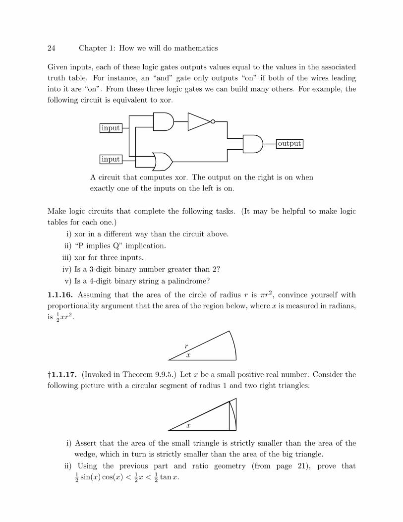
into it are “on”. From these three logic gates we can build many others. For example, the
following circuit is equivalent to xor.
input
input
output
A circuit that computes xor. The output on the right is on when
exactly one of the inputs on the left is on.
Make logic circuits that complete the following tasks. (It may be helpful to make logic
tables for each one.)
i) xor in a different way than the circuit above.
ii) “P implies Q” implication.
iii) xor for three inputs.
iv) Is a 3-digit binary number greater than 2?
v) Is a 4-digit binary string a palindrome?
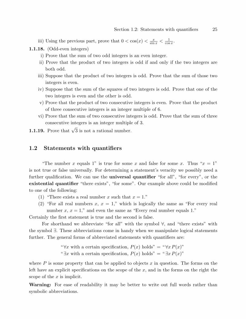
1.1.16. Assuming that the area of the circle of radius r is πr2, convince yourself with
proportionality argument that the area of the region below, where x is measured in radians,
is 12xr
2.
xr
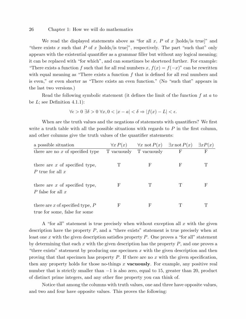
†1.1.17. (Invoked in Theorem 9.9.5.) Let x be a small positive real number. Consider the
following picture with a circular segment of radius 1 and two right triangles:
x
i) Assert that the area of the small triangle is strictly smaller than the area of the
wedge, which in turn is strictly smaller than the area of the big triangle.
ii) Using the previous part and ratio geometry (from page 21), prove that12 sin(x) cos(x) < 1
2x <12 tanx.
Section 1.2: Statements with quantifiers 25
iii) Using the previous part, prove that 0 < cos(x) < xsin x <
1cos x .
1.1.18. (Odd-even integers)
i) Prove that the sum of two odd integers is an even integer.
ii) Prove that the product of two integers is odd if and only if the two integers are
both odd.
iii) Suppose that the product of two integers is odd. Prove that the sum of those two
integers is even.
iv) Suppose that the sum of the squares of two integers is odd. Prove that one of the
two integers is even and the other is odd.
v) Prove that the product of two consecutive integers is even. Prove that the product
of three consecutive integers is an integer multiple of 6.
vi) Prove that the sum of two consecutive integers is odd. Prove that the sum of three
consecutive integers is an integer multiple of 3.
1.1.19. Prove that√
3 is not a rational number.
1.2 Statements with quantifiers
“The number x equals 1” is true for some x and false for some x. Thus “x = 1”
is not true or false universally. For determining a statement’s veracity we possibly need a
further qualification. We can use the universal quantifier “for all”, “for every”, or the
existential quantifier “there exists”, “for some”. Our example above could be modified
to one of the following:
(1) “There exists a real number x such that x = 1.”
(2) “For all real numbers x, x = 1,” which is logically the same as “For every real
number x, x = 1,” and even the same as “Every real number equals 1.”
Certainly the first statement is true and the second is false.
For shorthand we abbreviate “for all” with the symbol ∀, and “there exists” with
the symbol ∃. These abbreviations come in handy when we manipulate logical statements
further. The general forms of abbreviated statements with quantifiers are:
“ ∀x with a certain specification, P (x) holds” = “∀xP (x)”
“ ∃x with a certain specification, P (x) holds” = “∃xP (x)”
where P is some property that can be applied to objects x in question. The forms on the
left have an explicit specifications on the scope of the x, and in the forms on the right the
scope of the x is implicit.
Warning: For ease of readability it may be better to write out full words rather than
symbolic abbreviations.
26 Chapter 1: How we will do mathematics
We read the displayed statements above as “for all x, P of x [holds/is true]” and
“there exists x such that P of x [holds/is true]”, respectively. The part “such that” only
appears with the existential quantifier as a grammar filler but without any logical meaning;
it can be replaced with “for which”, and can sometimes be shortened further. For example:
“There exists a function f such that for all real numbers x, f(x) = f(−x)” can be rewritten
with equal meaning as “There exists a function f that is defined for all real numbers and
is even,” or even shorter as “There exists an even function.” (No “such that” appears in
the last two versions.)
Read the following symbolic statement (it defines the limit of the function f at a to
be L; see Definition 4.1.1):
∀ε > 0 ∃δ > 0 ∀x, 0 < |x− a| < δ ⇒ |f(x)− L| < ε.
When are the truth values and the negations of statements with quantifiers? We first
write a truth table with all the possible situations with regards to P in the first column,
and other columns give the truth values of the quantifier statements:
a possible situation ∀xP (x) ∀x notP (x) ∃xnotP (x) ∃xP (x)
there are no x of specified type T vacuously T vacuously F F
there are x of specified type,
P true for all x
T F F T
there are x of specified type,
P false for all x
F T T F
there are x of specified type, P
true for some, false for some
F F T T
A “for all” statement is true precisely when without exception all x with the given
description have the property P , and a “there exists” statement is true precisely when at
least one x with the given description satisfies property P . One proves a “for all” statement
by determining that each x with the given description has the property P , and one proves a
“there exists” statement by producing one specimen x with the given description and then
proving that that specimen has property P . If there are no x with the given specification,
then any property holds for those no-things x vacuously. For example, any positive real
number that is strictly smaller than −1 is also zero, equal to 15, greater than 20, product
of distinct prime integers, and any other fine property you can think of.
Notice that among the columns with truth values, one and three have opposite values,
and two and four have opposite values. This proves the following:

Section 1.2: Statements with quantifiers 27
Theorem 1.2.1. The negation of “ ∀xP (x)” is “ ∃x notP (x)”. The negation of “∃xP (x)”
is “ ∀x notP (x).”
Thus “∀xP (x)” is false if there is even one tiny tiniest example to the contrary.
“Every prime number is odd” is false because 2 is an even prime number. “Every whole
number divisible by 3 is divisible by 2” is false because 3 is divisible by 3 and is not divisible
by 2.
Remark 1.2.2. The statement “For all whole numbers x between 1/3 and 2/3, x2 is
irrational” is true vacuously. Another reason why “For all whole numbers x between 1/3
and 2/3, x2 is irrational” is true is that its negation, “There exists a whole number x
between 1/3 and 2/3 for which x2 is rational”, is false because there is no whole number
between 1/3 and 2/3: since the negation is false, we get yet more motivation to declare the
original statement true.
Exercises for Section 1.2
1.2.1. Show that the following statements are false by providing counterexamples.
i) No number is its own square.
ii) All numbers divisible by 7 are odd.
iii) The square root of all real numbers is greater than 0.
iv) For every real number x, x4 > 0.
1.2.2. Determine the truth value of the following statements, and justify your answers:
i) For all real numbers a, b, (a+ b)2 = a2 + b2.
ii) For all real numbers a, b, (a+ b)2 = a2 + 2ab+ b2.
iii) For all real numbers x < 5, x2 > 16.
iv) There exists a real number x < 5 such that x2 < 25.
v) There exists a real number x such that x2 = −4.
vi) There exists a real number x such that x3 = −8.
vii) For every real number x there exists a positive integer n such that xn > 0.
viii) For every real number x and every integer n, |x| < xn.
ix) For every integer m there exists an integer n such that m+ n is even.
x) There exists an integer m such that for all integers n, m+ n is even.
xi) For every integer n, n2 − n is even.
xii) Every list of 5 consecutive integers has one element that is a multiple of 5.
xiii) Every odd number is a multiple of 3.
28 Chapter 1: How we will do mathematics
1.2.3. Explain why the following statements have the same truth values:
i) There exists x such that there exists y such that P holds for the pair (x, y).
ii) There exists y such that there exists x such that P holds for the pair (x, y).
iii) There exists a pair (x, y) such that P holds for the pair (x, y).
1.2.4. Explain why the following statements have the same truth values:
i) ∀x > 0 ∀y > 0, xy > 0.
ii) ∀y > 0 ∀x > 0, xy > 0.
iii) ∀(x, y), x, y > 0 implies xy > 0.
1.2.5. (Contrast with the switching of quantifiers in the previous two exercises.) Explain
why the following two statements do not have the same truth values:
i) For every x > 0 there exists y > 0 such that xy = 1.
ii) There exists y > 0 such that for every x > 0, xy = 1.
1.2.6. Rewrite the following statements using quantifiers:
i) 7 is prime.
ii) There are infinitely many prime numbers.
iii) Everybody loves Raymond.
iv) Spring break is always in March.
1.2.7. Let “xLy” represent the statement that x loves y. Rewrite the following statements
symbolically: “Everybody loves somebody,” “Somebody loves everybody,” “Somebody is
loved by everybody,” “Everybody is loved by somebody.” At least one statement should
be of the form “∀x ∃y, xLy”. Compare its truth value with that of “∃x ∀y, xLy”.
1.2.8. Find a property P of real numbers x, y, z such that “∀y ∃x ∀z, P (x, y, z)” and
“∀z ∃x ∀y, P (x, y, z)” have different truth values.
1.2.9. Suppose that it is true that there exists x of some kind with property P . Can we
conclude that all x of that kind have property P? (A mathematician and a few other jokers
are on a train and see a cow through the window. One of them generalizes: “All cows in
this state are brown,” but the mathematician corrects: “This state has one cow whose one
side is brown.”)
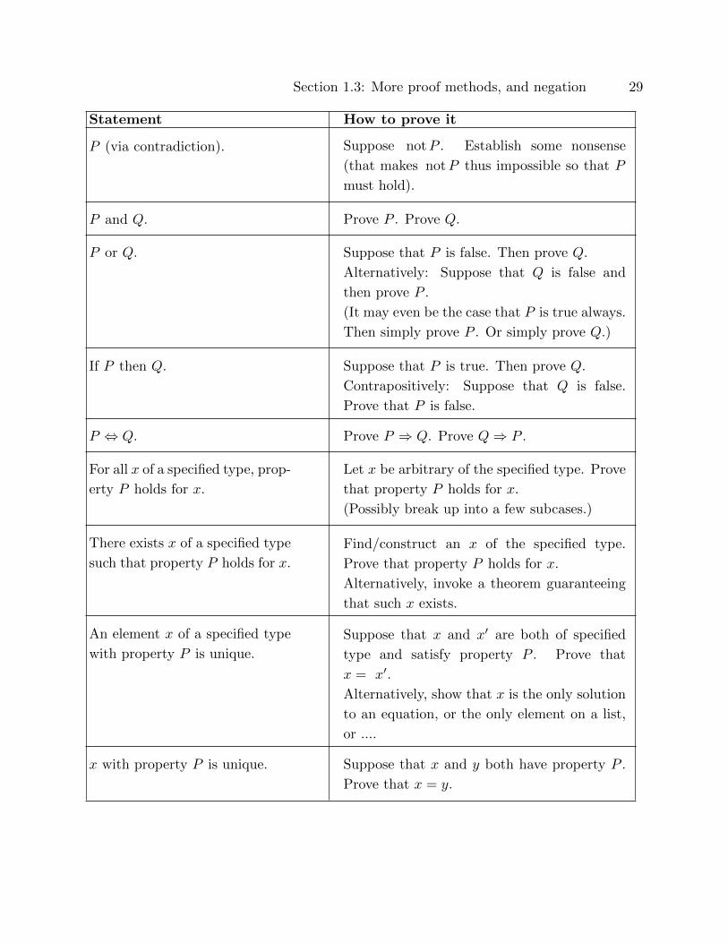
1.3 More proof methods, and negation
When statements are compound, they can be harder to prove. Fortunately, proofs
can be broken down into simpler statements. An essential chart of this breaking down is
in the chart on the next page.
Section 1.3: More proof methods, and negation 29
Statement How to prove it
P (via contradiction). Suppose notP . Establish some nonsense
(that makes notP thus impossible so that P
must hold).
P and Q. Prove P . Prove Q.
P or Q. Suppose that P is false. Then prove Q.
Alternatively: Suppose that Q is false and
then prove P .
(It may even be the case that P is true always.
Then simply prove P . Or simply prove Q.)
If P then Q. Suppose that P is true. Then prove Q.
Contrapositively: Suppose that Q is false.
Prove that P is false.
P ⇔ Q. Prove P ⇒ Q. Prove Q⇒ P .
For all x of a specified type, prop-
erty P holds for x.
Let x be arbitrary of the specified type. Prove
that property P holds for x.
(Possibly break up into a few subcases.)
There exists x of a specified type
such that property P holds for x.
Find/construct an x of the specified type.
Prove that property P holds for x.
Alternatively, invoke a theorem guaranteeing
that such x exists.
An element x of a specified type
with property P is unique.
Suppose that x and x′ are both of specified
type and satisfy property P . Prove that
x = x′.
Alternatively, show that x is the only solution
to an equation, or the only element on a list,
or ....
x with property P is unique. Suppose that x and y both have property P .
Prove that x = y.
30 Chapter 1: How we will do mathematics
Example 1.3.1. Prove that 2 and 3 are prime integers. (Prove that 2 is a prime integer
and that 3 is a prime integer.)
Proof. Let m and n be whole numbers strictly greater than 1. If m · n = 2, then 1 <
m,n ≤ 2, so m = n = 2, but 2 · 2 is not equal to 2. Thus 2 cannot be written as a product
of two positive numbers different from 1, so 2 is a prime number. If instead m ·n = 3, then
1 < m,n ≤ 3. Then all combinations of products are 2 · 2, 2 · 3, 3 · 2, 3 · 3, none of which
is 3. Thus 3 is a prime number.
Example 1.3.2. Prove that a positive prime number is either odd or it equals 2. (One
may think of −2 as a prime number as well, that is why “positive” appears. But often the
term “prime” implicitly assumes positivity.)
Proof. Let p be a positive prime number. Suppose that p is not odd. Then p must be even.
Thus p = 2 · q for some positive whole number q. Since p is a prime, it follows that q = 1,
so that p = 2.
Example 1.3.3. Prove that if an integer is a multiple of 2 and a multiple of 3, then it is
a multiple of 6. (Implicit here is that the factors are integers.)
Proof. Let n be an integer that is a multiple of 2 and of 3. Write n = 2 · p and n = 3 · q for
some integers p and q. Then 2 · p = 3 · q is even, which forces that q must be even. Hence
q = 2 · r for some integer r, so that n = 3 · q = 3 · 2 · r = 6 · r. Thus n is a multiple of 6.
Example 1.3.4. Prove that for all real numbers x, x2 = (−x)2.
Proof. Let x be an arbitrary real number. Then (−x)2 = (−x)(−x) = (−1)x(−1)x =
(−1)(−1)x x = 1 · x2 = x2.Example 1.3.5. Prove that there exists a real number x such that x3 − 3x = 2.
Proof. Observe that 2 is a real number and that 23 − 3 · 2 = 2. Thus x = 2 satisfies the
conditions.
Example 1.3.6. Prove that there exists a real number x such that x3 − x = 1.
Proof. Observe that f(x) = x3 − x is a continuous function. Since 1 is strictly between
f(0) = 0 and f(2) = 6, by the Intermediate value theorem (Theorem 5.3.1 in these notes)
[invoking a theorem rather than constructing x, as opposed to in the previ-
ous example]* there exists a real number x strictly between 0 and 2 such that f(x) = 1.
* Recall that this font in brackets and in red color indicates the reasoning that should go on in the
background in your head; these statements are not part of a proof.

Section 1.3: More proof methods, and negation 31
Example 1.3.7. (Mixture of methods) For every real number x strictly between 0 and 1
there exists a positive real number y such that 1x + 1
y = 1xy .
Proof. [We have to prove that for all x as specified some property holds.]
Let x be in (0, 1). [For this x we have to find y ...] Set y = 1 − x. [Was this
a lucky find? No matter how we got inspired to determine this y, we now
verify that the stated properties hold for x and y.] Since x is strictly smaller
than 1, it follows that y is positive. Thus also xy is positive, and y+ x = 1. After dividing
the last equation by the positive number xy we get that 1x + 1
y = 1xy .
Furthermore, y in the previous example is unique: it has no choice but to be 1− x.
Example 1.3.8. (The Fundamental theorem of arithmetic) Any positive integer
n > 1 can be written as pa11 pa22 · · · pakk for some positive prime integers p1 < · · · < pk and
some positive integers a1, . . . , ak. (Another standard part of the Fundamental theorem of
arithmetic is that the pi and the ai are unique, but we do not prove that. Once you are
comfortable with proofs you can prove that part yourself.)
Proof. (This proof is harder than most proofs in this book; you may want to skip it.)
Suppose for contradiction that the conclusion fails for some positive integer n. Then on
the list 2, 3, 4, . . . , n let m be the smallest integer for which the conclusion fails. If m is
a prime, take k = 1 and p1 = m, a1 = 1, and so the conclusion does not fail. Thus m
cannot be a prime number, and so m = m1m2 for some positive integers m1,m2 strictly
bigger than 1. Necessarily 2 ≤ m1,m2 < m. By the choice of m, the conclusion is true
for m1 and m2. Write m1 = pa11 pa22 · · · pakk and m2 = qb11 q
b22 · · · q
bll for some positive prime
integers p1 < · · · < pk, q1 < · · · < qk and some positive integers a1, . . . , ak, b1, . . . , bl. Thus
m = pa11 pa22 · · · pakk q
b11 q
b22 · · · q
bll is a product of positive prime numbers, and after sorting
and merging the pi and qj , the conclusion follows also for m. But we assumed that the
conclusion fails for m, which yields the desired contradiction. Hence the conclusion does
not fail for any positive integer.
Example 1.3.9. Any positive rational number can be written in the form ab , where a
and b are positive whole numbers, and in any prime factorizations of a and b as in the
previous example, the prime factors for a are distinct from the prime factors for b.
Proof. [We have to prove that for all ...] Let x be a(n arbitrary) positive rational
number. [We rewrite the meaning of the assumption next in a more concrete
and usable form.] Thus x = ab for some whole numbers a, b. If a is negative, since x
is positive necessarily b has to be negative. But then −a,−b are positive numbers, and
x = −a−b . Thus by possibly replacing a, b with −a,−b we may assume that a, b are positive.
[A rewriting trick.] There may be many different pairs of a, b, and we choose a pair for
32 Chapter 1: How we will do mathematics
which a is the smallest of all possibilities. [A choosing trick. But does the smallest
a exist?] Such a does exist because in a collection of given positive integers there is always
a smallest one. Suppose that a and b have a (positive) prime factor p in common. Write
a = a0p and b = b0p for some positive whole numbers a0, b0. Then x = a0b0
, and since
0 < a0 < a, this contradicts the choice of the pair a, b. Thus a and b could not have had a
prime factor in common.
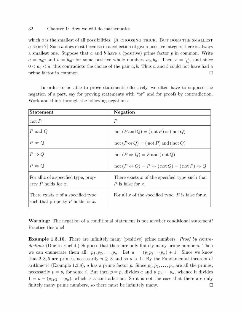
In order to be able to prove statements effectively, we often have to suppose the
negation of a part, say for proving statements with “or” and for proofs by contradiction.
Work and think through the following negations:
Statement Negation
notP P
P and Q not (P andQ) = ( notP ) or ( notQ)
P or Q not (P orQ) = ( notP ) and ( notQ)
P ⇒ Q not (P ⇒ Q) = P and ( notQ)
P ⇔ Q not (P ⇔ Q) = P ⇔ ( notQ) = ( notP )⇔ Q
For all x of a specified type, prop-
erty P holds for x.
There exists x of the specified type such that
P is false for x.
There exists x of a specified type
such that property P holds for x.
For all x of the specified type, P is false for x.
Warning: The negation of a conditional statement is not another conditional statement!
Practice this one!
Example 1.3.10. There are infinitely many (positive) prime numbers. Proof by contra-
diction: (Due to Euclid.) Suppose that there are only finitely many prime numbers. Then
we can enumerate them all: p1, p2, . . . , pn. Let a = (p1p2 · · · pn) + 1. Since we know
that 2, 3, 5 are primes, necessarily n ≥ 3 and so a > 1. By the Fundamental theorem of
arithmetic (Example 1.3.8), a has a prime factor p. Since p1, p2, . . . , pn are all the primes,
necessarily p = pi for some i. But then p = pi divides a and p1p2 · · · pn, whence it divides
1 = a − (p1p2 · · · pn), which is a contradiction. So it is not the case that there are only
finitely many prime numbers, so there must be infinitely many.

Section 1.3: More proof methods, and negation 33
Another proof by contradiction: (Due to R. Mestrovic, American Mathematical
Monthly 124 (2017), page 562.) Suppose that there are only finitely many prime numbers.
Then we can enumerate them all: p1 = 2, p2 = 3, . . . , pn. The positive integer p2p3 · · · pn−2
has no odd prime factors, and since it is odd, it must be equal to 1. Hence p2p3 · · · pn = 3,
which is false since p2 = 3, p3 = 5, and so on.
Exercises for Section 1.3
1.3.1. Prove that every whole number is either odd or even.
1.3.2. Prove that the successor of any odd integer is even.
1.3.3. Prove that if n is an even integer, then either n is a multiple of 4 or n/2 is odd.
1.3.4. Prove that if 0 < x < 1, then x2 < x <√x.
1.3.5. Prove that if 1 < x, then√x < x < x2.
1.3.6. Prove that there exists a real number x such that x2 + 512x = 1
6 .
1.3.7. Prove that the following pairs of statements are negations of each other:
i) P ⇔ Q.
(P andQ) or ( notP and notQ).
ii) P and (P ⇒ Q).
notP or notQ.
iii) (P ⇒ notQ) and (R⇒ Q).
(P andQ) or (R and notQ).
iv) P and (Q or notR).
P ⇒ ( notQ andR).
1.3.8. Why are “f is continuous at all points” and “f is not continuous at 3” not negations
of each other?
1.3.9. Why are “Some continuous functions are differentiable” and “All differentiable func-
tions are continuous” not negations of each other?
1.3.10. Why is “P ⇒ notQ” not the negation of “P ⇒ Q”?
1.3.11. Negate the following statements:
i) The function f is continuous at 5.
ii) If x > y then x > z.
iii) For every ε > 0, there exists δ > 0 such that f(δ) = ε.
iv) For every ε > 0, there exists δ > 0 such that for all x, f(x · δ) = εx.
v) For every ε > 0, there exists δ > 0 such that for all x, 0 < |x − a| < δ implies
|f(x)− L| < ε.
34 Chapter 1: How we will do mathematics
1.3.12. Find at least three functions f such that for all real numbers x, f(x2) = x2.
1.3.13. Prove that f(x) = x is the unique function that is defined for all real numbers
and that has the property that for all x, f(x3) = x3.
1.3.14. Prove that the following are false:
i) For every real number x there exists a real number y such that xy = 1.
ii) 5n + 2 is prime for all non-negative integers n.
iii) For every real number x, if x2 > 4 then x > 2.
iv) For every real number x,√x2 = x.
v) The cube of every real number is positive.
vi) The square of every real number is positive.
1.3.15. Prove that there exists a real number y such that for all real numbers x, xy = y.
1.3.16. Prove that there exists a real number y such that for all real numbers x, xy = x.
1.3.17. Prove that for every real number x there exists a real number y such that x+y = 0.
1.3.18. Prove that there exists no real number y such that for all real numbers x, x+y = 0.
1.3.19. Prove that for every real number y there exists a real number x such that x+y 6= 0.
1.4 Summation
There are many reasons for not writing out the sum of the first hundred numbers
in full length with 100 numbers and 99 plus signs: it would be too long, it would not
be any clearer, we would probably start doubting the intelligence of the writer, it would
waste paper and ink... The clear and short way of writing such a long sum is with the
summation sign Σ:100∑k=1
k or
100∑n=1
n.
The counters k and n above are dummy variables, they vary from 1 to 100. We could use any
other name in place of k or n. In general, if f is a function defined at m,m+1,m+2, . . . , n,
we use the summation sign for shortening as follows:
n∑k=m
f(k) = f(m) + f(m+ 1) + f(m+ 2) + · · ·+ f(n).
This is one example where a good notation saves space (and it even sometimes clarifies
the concept). Typographically, when summation is displayed, the two bounds (m and n)
appear below and above the summation sign, but when the summation is in-line, the two
bounds appear to the right of the sign, like so:∑nk=m f(k). (This prevents lines jamming
into each other.)
Section 1.4: Summation 35
Now is a good time to discuss polynomials. A polynomial function is a function
of the form f(x) = a0 + a1x + · · · + anxn for some non-negative integer n and some
numbers a0, a1, . . . , an. We call a0 + a1x+ · · ·+ anxn a polynomial, and if an is non-zero,
we say that the polynomial has degree n. (More on the degrees of polynomial functions
is in Example 1.5.5, Exercise 2.6.14.) It is convenient to write this polynomial with the
shorthand notation
f(x) = a0 + a1x+ · · ·+ anxn =
n∑k=0
akxk.
Here, of course, x0 stands for 1. When we evaluate f at 0, we get a0 = a0+a1 ·0+· · ·+an ·0n
=∑nk=0 ak0k, and we deduce that notationally 00 stands for 1 here.
Remark 1.4.1. 00 could possibly be thought of also as limx→0+
0x, which is surely equal to 0.
But then, is 00 equal to 0 or 1 or to something else entirely? Well, it turns out that 00
is not equal to that zero limit – you surely know of other functions f for which limx→c
f(x)
exists but the limit is not equal to f(c). (Check out also Exercise 7.6.9.)
Examples 1.4.2.
(1)5∑k=1
2 = 2 + 2 + 2 + 2 + 2 = 10.
(2)
5∑k=1
k = 1 + 2 + 3 + 4 + 5 = 15.
(3)4∑k=1
k2 = 12 + 22 + 32 + 42 = 30.
(4)12∑k=10
cos(kπ) = cos(10π) + cos(11π) + cos(12π) = 1− 1 + 1 = 1.
(5)
2∑k=−1
(4k3) = −4 + 0 + 4 + 4 · 8 = 32 = 4(−1 + 0 + 1 + 1 · 8) = 4
2∑k=−1
k3.
(6)n∑k=1
3 = 3 added to itself n times = 3n.
(7)b∑
k=a
2 = 2 added to itself b− a+ 1 times = 2(b− a+ 1).
We can even deal with empty sums such as∑0k=1 ak: here the index starts at k = 1
and keeps increasing and we stop at k = 0, but there are no such indices k. What could
possibly be the meaning of such an empty sum? Note that
4∑k=1
ak =2∑k=1
ak +4∑k=3
ak =1∑k=1
ak +4∑k=2
ak =0∑k=1
ak +4∑k=1
ak,

36 Chapter 1: How we will do mathematics
or explicitly written out:
a1 + a2 + a3 + a4 = (a1 + a2) + (a3 + a4) = (a1) + (a2 + a3 + a4) = () + (a1 + a2 + a3 + a4),
from which we deduce that this empty sum must be 0. Similarly, every empty sum equals 0.
Similarly we can shorten products with the product sign Π:
n∏k=m
f(k) = f(m) · f(m+ 1) · f(m+ 2) · · · · · f(n).
In particular, for all non-negative integers n, the product∏nk=1 k is used often and is
abbreviated as n! =∏nk=1 k. See Exercise 1.4.6 for the fact that 0! = 1.
Exercises for Section 1.4
1.4.1. Compute∑4k=0(2k + 1),
∑4k=0(k2 + 2).
1.4.2. Determine all non-negative integers n for which∑nk=0 k =
∑nk=0 n.
1.4.3. Prove that
i) cn∑
k=m
f(k) =n∑
k=m
cf(k).
ii)
n∑k=m
f(k) +
n∑k=m
g(k) =
n∑k=m
(f(k) + g(k)).
1.4.4. Prove that∑0k=1 k = 0·(−1)
2 .
1.4.5. Prove that for all integers m ≤ n,m−1∑k=1
f(k) +n∑
k=m
f(k) =n∑k=1
f(k).
1.4.6. Prove that the empty product equals 1. In particular, it follows that we can declare
0! = 1. This turns out to be very helpful notationally.
1.4.7. Prove:
i)5∏k=1
2 = 32.
ii)5∏k=1
k = 120.
Section 1.5: Proofs by (mathematical) induction 37
1.5 Proofs by (mathematical) induction
So far we have learned a few proof methods. There is another type of proofs that
deserves special mention, and this is proof by (mathematical) induction, sometimes
referred to as the principle of mathematical induction. This method can be used when
one wants to prove that a property P holds for all integers n greater than or equal to an
integer n0. Typically, n0 is either 0 or 1, but it can be any integer, even a negative one.
Induction is a two-step procedure:
(1) Base case: Prove that P holds for n0.
(2) Inductive step: Let n > n0. Assume that P holds for all integers n0, n0 +1, n0 +
2, . . . , n− 1. Prove that P holds for n.
Why does induction succeed in proving that P holds for all n ≥ n0? By the base
case we know that P holds for n0. The inductive step then proves that P also holds for
n0 + 1. So then we know that the property holds for n0 and n0 + 1, whence the inductive
step implies that it also holds for n0 + 2. So then the property holds for n0, n0 + 1 and
n0 +2, whence the inductive step implies that it also holds for n0 +3. This establishes that
the property holds for n0, n0 + 1, n0 + 2, and n0 + 3, so that by inductive step it also holds
for n0 + 4. We keep going. For any integer n > n0, in n − n0 step we similarly establish
that the inductive step holds for n0, n0 + 1, n0 + 2, . . . , n0 + (n − n0) = n. Thus for any
integer n ≥ n0, we eventually prove that P holds for it.
The same method can be phrased with a slightly different two-step process, with the
same result, and the same name:
(1) Base case: Prove that P holds for n0.
(2) Inductive step: Let n > n0. Assume that P holds for integer n− 1. Prove that
P holds for n.
Similar reasoning as in the previous case also shows that this induction principle
succeeds in proving that P holds for all n ≥ n0.
Example 1.5.1. Prove the equality∑nk=1 k = n(n+1)
2 for all n ≥ 1.
Proof. Base case n = 1: The left side of the equation is∑1k=1 k which equals 1. The right
side is 1(1+1)2 which also equals 1. This verifies the base case.
Inductive step: Let n > 1 and we assume that the equality holds for n − 1. [We
want to prove the equality for n. We start with the expression on the
left (messier) side of the desired and not-yet-proved equation for n and
manipulate the expression until it resembles the desired right side.] Then
n∑k=1
k =
(n−1∑k=1
k
)+ n
38 Chapter 1: How we will do mathematics
=(n− 1)(n− 1 + 1)
2+ n (by induction assumption for n− 1)
=n2 − n
2+
2n
2(by algebra)
=n2 + n
2
=n(n+ 1)
2,
as was to be proved.
We can even prove the equality∑nk=1 k = n(n+1)
2 for all n ≥ 0. Since we have already
proved this equality for all n ≥ 1, it remains to prove it for n = 0. The left side∑0k=1 k is
an empty sum and hence 0, and the right side is 0(0+1)2 , which is also 0.
Example 1.5.2. Prove the equality∑nk=1 k(k + 1)(k + 2)(k + 3) = n(n+1)(n+2)(n+3)(n+4)
5
for all n ≥ 1.
Proof. Base case n = 1:
1∑k=1
k(k + 1)(k + 2)(k + 3) = 1(1 + 1)(1 + 2)(1 + 3) = 1 · 2 · 3 · 4
=1 · 2 · 3 · 4 · 5
5=
1(1 + 1)(1 + 2)(1 + 3)(1 + 4)
5,
which verifies the base case.
Inductive step: Let n > 1 and we assume that the equality holds for n − 1. [We
want to prove the equality for n. We start with the expression on the
left side of the desired and not-yet-proved equation for n (the messier of
the two) and manipulate the expression until it resembles the desired right
side.] Then
n∑k=1
k(k + 1)(k + 2)(k + 3) =
(n−1∑k=1
k(k + 1)(k + 2)(k + 3)
)+ n(n+ 1)(n+ 2)(n+ 3)
=(n− 1)(n− 1 + 1)(n− 1 + 2)(n− 1 + 3)(n− 1 + 4)
5+ n(n+ 1)(n+ 2)(n+ 3)
(by induction assumption)
=(n− 1)n(n+ 1)(n+ 2)(n+ 3)
5+
5n(n+ 1)(n+ 2)(n+ 3)
5(by algebra)
=n(n+ 1)(n+ 2)(n+ 3)
5(n− 1 + 5) (by factoring)
=n(n+ 1)(n+ 2)(n+ 3)(n+ 4)
5,
as was to be proved.
Section 1.5: Proofs by (mathematical) induction 39
Example 1.5.3. Assuming that the derivative of x is 1 and the product rule for deriva-
tives, prove that for all n ≥ 1, ddx (xn) = nxn−1. (We introduce derivatives formally in
Section 6.1.)
Proof. We start the induction at n = 1. By calculus we know that the derivative of x1 is
1 = 1 · x0 = 1 · x1−1, so equality holds in this case.
Inductive step: Suppose that equality holds for 1, 2, . . . , n− 1. Then
d
dx(xn) =
d
dx(x · xn−1)
=d
dx(x) · xn−1 + x
d
dx(xn−1) (by the product rule of differentiation)
= 1 · xn−1 + (n− 1)x · xn−2 (by induction assumption for 1 and n− 1)
= xn−1 + (n− 1)xn−1
= nxn−1.
The following result will be needed many times, so remember it well.
Example 1.5.4. For any number x and any integer n ≥ 1,
(1− x)(1 + x+ x2 + x3 + · · ·+ xn) = 1− xn+1.
Proof. When n = 1,
(1− x)(1 + x+ x2 + x3 + · · ·+ xn) = (1− x)(1 + x) = 1− x2 = 1− xn+1,
which proves the base case. Now suppose that equality holds for some integer n − 1 ≥ 1.
Then
(1− x)(1 + x+ x2 + · · ·+ xn−1 + xn) = (1− x)((1 + x+ x2 + · · ·+ xn−1) + xn
)= (1− x)(1 + x+ x2 + · · ·+ xn−1) + (1− x)xn
= 1− xn + xn − xn+1 (by induction assumption and algebra)
= 1− xn+1,
which proves the inductive step.
Example 1.5.5. (Euclidean algorithm) Let f(x) = a0 + a1x + · · · + anxn for some
numbers a0, a1, . . . , an and with an 6= 0, and let g(x) = b0 + b1x + · · · + bmxm for some
numbers b0, b1, . . . , bm and with bm 6= 0. Suppose that m,n ≥ 1. Then there exist polyno-
mials q(x) and r(x) such that f(x) = q(x) · g(x) + r(x) and such that the degree of r(x) is
strictly smaller than m.
Proof. We keep g(x) fixed and we prove by induction on the degree n of f(x) that the claim
holds for all polynomials f(x). If n < m, then we are done with q(x) = 0 and r(x) = f(x).
40 Chapter 1: How we will do mathematics
If n = m, then we set q(x) = anbn
and (necessarily)
r(x) = f(x)− ambm
g(x) = a0 + a1x+ · · ·+ amxm − am
bm(b0 + b1x+ · · ·+ bmx
m)
= (a0 −ambm
b0) + (a1 −ambm
b1)x+ (a2 −ambm
b2)x2 + · · ·+ +(am−1 −ambm
bm−1)xm−1,
which has degree strictly smaller than m. These are the base cases.
Now suppose that n > m. Set h(x) = a1 + a2x+ a3x2 + · · ·+ anx
n−1. By induction
on n, there exist polynomials q1(x) and r1(x) such that h(x) = q1(x) ·g(x)+r1(x) and such
that the degree of r1(x) is strictly smaller than m. Then xh(x) = xq1(x) · g(x) + xr1(x).
Since the degree of xr1(x) is at most m, by the second base case there exist polynomials
q2(x) and r2(x) such that xr1(x) = q2(x)g(x) + r2(x) and such that the degree of r2(x) is
strictly smaller than m. Now set q(x) = xq1(x) + q2(x) and r(x) = r2(x) + a0. Then the
degree of r(x) is strictly smaller than m, and
q(x)g(x) + r(x) = xq1(x)g(x) + q2(x)g(x) + r2(x) + a0
= xq1(x)g(x) + xr1(x) + a0
= xh(x) + a0
= f(x).
Remark 1.5.6. A common usage of the Euclidean algorithm is in finding the greatest
common divisor of two polynomials. A polynomial d(x) divides f(x) and g(x) exactly
when it divides g(x) and r(x) = f(x)−q(x) ·g(x). It is easier to find factors of polynomials
of smaller degree. As an example, let f(x) = x4+4x3+6x2+4x+1 and g(x) = x3+2x2+x.
The first step of the Euclidean algorithm gives
r(x) = f(x)− (x+ 2)g(x) = x2 + 2x+ 1.
So to find the greatest common divisor of f(x) and g(x) it suffices to find the greatest
common divisor of g(x) and r(x). The Euclidean algorithm on these two gives r1(x) =
g(x) − xr(x) = 0, so that to find the greatest common divisor of f(x) and g(x) it suffices
to find the greatest common divisor of r(x) and 0. But the latter is clearly r(x). In fact,
f(x) = (x+ 1)4 and g(x) = x(x+ 1)2.
Example 1.5.7. For all positive integers n, n√n < 2.
Proof. Base case: n = 1, so n√n = 1 < 2.
Inductive step: Suppose that n is an integer with n ≥ 2 and that n−1√n− 1 < 2.
This means that n− 1 < 2n−1. Hence n < 2n−1 + 1 < 2n−1 + 2n−1 = 2 · 2n−1 = 2n, so thatn√n < 2.

Section 1.5: Proofs by (mathematical) induction 41
Remark 1.5.8. There are two other equivalent formulations of mathematical induction
for proving a property P for all integers n ≥ n0:
Mathematical induction, version III:
(1) Base case: Prove that P holds for n0.
(2) Inductive step: Let n ≥ n0. Assume that P holds for all integers n0, n0 +
1, n0 + 2, . . . , n. Prove that P holds for n+ 1.
Mathematical induction, version IV:
(1) Base case: Prove that P holds for n0.
(2) Inductive step: Let n ≥ n0. Assume that P holds for integer n. Prove that P
holds for n+ 1.
Convince yourself that these two versions of the workings of mathematical induction
differ from the original two versions only in notation.
Exercises for Section 1.5: Prove the following properties for n ≥ 1 by induction.
1.5.1.n∑k=1
k2 =n(n+ 1)(2n+ 1)
6.
1.5.2.
n∑k=1
k3 =
(n(n+ 1)
2
)2
.
1.5.3. The sum of the first n odd positive integers is n2.
1.5.4.n∑k=1
(2k − 1) = n2.
1.5.5. (Triangle inequality) For all positive integers n and for all real numbers a1, . . . , an,
|a1 + a2 + · · ·+ an| ≤ |a1|+ |a2|+ · · ·+ |an|. (Hint: there may be more than one base case.
Why is that?)
1.5.6.n∑k=1
(3k2 − k) = n2(n+ 1).
1.5.7. 1 · 2 + 2 · 3 + 3 · 4 + · · ·+ n(n+ 1) = 13n(n+ 1)(n+ 2).
1.5.8. 7n + 2 is a multiple of 3.
1.5.9. 3n−1 < (n+ 1)!.
1.5.10.1√1
+1√2
+1√3
+ · · ·+ 1√n≥√n.
1.5.11.1
12+
1
22+
1
32+ · · ·+ 1
n2≤ 2− 1
n.

42 Chapter 1: How we will do mathematics
1.5.12. Let a1 = 2, and for n ≥ 2, an = 3an−1. Formulate and prove a theorem giving an
in terms of n (no dependence on other ai).
1.5.13. 8 divides 5n + 2 · 3n−1 + 1.
1.5.14. 1(1!) + 2(2!) + 3(3!) + · · ·+ n(n!) = (n+ 1)!− 1.
1.5.15. 2n−1 ≤ n!.
1.5.16.n∏k=2
(1− 1
k
)=
1
n.
1.5.17.n∏k=2
(1− 1
k2
)=n+ 1
2n.
1.5.18.
n∑k=0
2k(k + 1) = 2n+1n+ 1.
1.5.19.∑2n
k=11k ≥
n+22 .
†1.5.20. (This is invoked in Example 9.1.9.)∑2n−1k=1
1k2 ≤
∑nk=0
12k
.
†1.5.21. (This is invoked in the proof of Theorem 9.4.1.) For all numbers x, y, xn − yn =
(x− y)(xn−1 + xn−2y + xn−3y2 + · · ·+ yn−1
)= (x− y)
∑n−1k=0 x
n−1−kyk.
†1.5.22. (This is invoked in the Ratio tests Theorems 8.6.6 and 9.2.3.) Let r be a positive
real number. Suppose that for all positive integers n ≥ n0, an+1 < ran. Prove that for
all positive integers n > n0, an < rn−n0an0. (The strict relationship < between the ai can
also be replaced by ≤, >, ≥ throughout.)
1.5.23. Let An = 12 + 22 + 32 + · · ·+ (2n− 1)2 and Bn = 12 + 32 + 52 + · · ·+ (2n− 1)2.
Find formulas for An and Bn, and prove them (by using algebra and previous problems,
and possibly not with induction).
1.5.24. (From the American Mathematical Monthly 123 (2016), page 87, by K. Gaitanas)
Prove that for every n ≥ 2,∑n−1k=1
k(k+1)! = 1− 1
n! .
1.5.25. Let An = 11·2 + 1
2·3 + 13·4 + · · ·+ 1
n(n+1) . Find a formula for An and prove it.
1.5.26. There are exactly n people at a gathering. Everybody shakes everybody else’s
hands exactly once. How many handshakes are there?
1.5.27. Find with proof an integer n0 such that n2 < 2n for all integers n ≥ n0.
1.5.28. Find with proof an integer n0 such that 2n < n! for all integers n ≥ n0.
1.5.29. Let x be a real number. For any positive integer n define Sn = 1+x+x2 +· · ·+xn.
i) Prove that for any n ≥ 2, xSn−1 + 1 = Sn, and that Sn(1− x) = 1− xn+1.
ii) Prove that if x = 1, then Sn = n+ 1.
iii) Prove that if x 6= 1, then Sn = 1−xn+1
1−x . Compare with the proof by induction in
Example 1.5.4.
Section 1.5: Proofs by (mathematical) induction 43
1.5.30. (Fibonacci numbers) Let s1 = 1, s2 = 1, and for all n ≥ 2, let sn+1 = sn+sn−1.
This sequence starts with 1, 1, 2, 3, 5, 8, 13, 21, 34, . . .. (Many parts below are taken from the
book Fibonacci Numbers by N. N. Vorob’ev, published by Blaisdell Publishing Company,
1961, translated from the Russian by Halina Moss; there is a new edition of the book with
author’s last name written as Vorobiev, published by Springer Basel AG, 2002, translated
from the Russian by Mircea Martin.)
i) Fibonacci numbers are sometimes “motivated” as follows. You get the rare gift of
a pair of newborn Fibonacci rabbits. Fibonacci rabbits are the type of rabbits who
never die and each month starting in their second month produce another pair of
rabbits. At the beginning of months one and two you have exactly that 1 pair of
rabbits. In the second month, that pair gives you another pair of rabbits, so at
the beginning of the third month you have 2 pairs of rabbits. In the third month,
the original pair produces another pair of rabbits, so that at the beginning of the
fourth month, you have 3 pairs of rabbits. Justify why the number of rabbits at
the beginning of the nth month is sn.
ii) Prove that for all n ≥ 1, sn = 1√5
(1+√
52
)n− 1√
5
(1−√
52
)n. (It may seem amazing
that these expressions with square roots of 5 always yield positive integers.) Note
that the base case requires proving this for n = 1 and n = 2, and that the inductive
step uses knowing the property for the previous two integers.
iii) Prove that s1 + s3 + s5 + · · ·+ s2n−1 = s2n.
iv) Prove that s2 + s4 + s6 + · · ·+ s2n = s2n+1 − 1.
v) Prove that s1 + s2 + s3 + · · ·+ sn = sn+2 − 1.
vi) Prove that s1 − s2 + s3 − s4 + · · ·+ s2n−1 − s2n = 1− s2n−1.
vii) Prove that s1 − s2 + s3 − s4 + · · ·+ s2n−1 − s2n + s2n+1 = s2n + 1.
viii) Prove that s1 − s2 + s3 − s4 + · · ·+ (−1)n+1sn = (−1)n+1sn−1 + 1.
ix) Prove that for all n ≥ 3, sn > ( 1+√
52 )n−2.
x) Prove that for all n ≥ 1, s21 + s2
2 + · · ·+ s2n = snsn+1.
xi) Prove that sn+1sn−1 − s2n = (−1)n.
xii) Prove that s1s2 + s2s3 + · · ·+ s2n−1s2n = s22n.
xiii) Prove that s1s2 + s2s3 + · · ·+ s2ns2n+1 = s22n+1 − 1.
xiv) Prove that ns1 + (n− 1)s2 + (n− 2)s3 + · · ·+ 2sn−1 + sn = sn+4 − (n+ 3).
xv) Prove that for all n ≥ 1 and all k ≥ 2, sn+k = sksn+1 + sk−1sn.
xvi) Prove that for all n, k ≥ 1, skn is a multiple of sn. (Use the previous part.)
xvii) Prove that s2n+1 = s2n+1 + s2
n.
xviii) Prove that s2n = s2n+1 − s2
n−1.
xix) Prove that s3n = s3n+1 + s3
n − s3n−1.
xx) Prove that sn+1 =(
1+√
52
)sn +
(1−√
52
)n.

44 Chapter 1: How we will do mathematics
xxi) Prove that s3 + s6 + s9 + · · ·+ s3n = s3n+2−12 . (Use the previous part.)
xxii) Prove that s31 + s3
2 + s33 + · · ·+ s3
n = s3n+2+(−1)n+16sn−1+510 .
xxiii) Prove that
∣∣∣∣∣sn − (1 +√
5)n
2n√
5
∣∣∣∣∣ < 1
2.
(xxiv)* If you know a bit of number theory, prove that for all positive integers m,n, the
greatest common divisor of sm and sn is sgcd(m,n).
(xxv)* Prove that sn is even if and only if n is a multiple of 3. Prove that sn is divisible
by 3 if and only if n is a multiple of 4. Prove that sn is divisible by 4 if and only
if n is a multiple of 6. Prove that sn is divisible by 5 if and only if n is a multiple
of 5. Prove that sn is divisible by 7 if and only if n is a multiple of 8. Prove that
there are no Fibonacci numbers that have the remainder of 4 when divided by 8.
Prove that there are no odd Fibonacci numbers that are divisible by 17.
xxvi) If you know matrices, prove that for all n ≥ 2,
[1 11 0
]n=
[sn+1 snsn sn−1
].
1.5.31. (Via the grapevine, based on ideas of Art Benjamin, Harvey Mudd College, and
Dan Velleman, Amherst College) A tromino is a plane figure composed of three squares in
L-shape:
Prove that for every positive integer n, any 2n × 2n square grid with exactly one of the
squares removed can be tiled with trominoes.
1.5.32. Pick a vertex V in a triangle. Draw n distinct lines from V to the opposite edge
of the triangle. If n = 1, you get the original triangle and two smaller triangles, for a total
of three triangles. Determine the number of distinct triangles obtained in this way with
arbitrary n.
1.5.33. (Spiral of Theodorus) Draw a triangle with vertices at (0, 0), (1, 0), (1, 1). The
hypotenuse has length√
2.
i) One of the vertices of the hypotenuse is at (0, 0). At the other vertex of the
hypotenuse, draw an edge of length 1 at a right angle away from the first triangle.
Make a triangle from the old hypotenuse and this new edge. What is the length of
the hypotenuse of the new triangle?
ii) Repeat the previous step twice.
iii) Argue by induction that one can draw the square root of every positive integer.

Section 1.6: Pascal’s triangle 45
1.5.34. (Tower of Hanoi) There are 3 pegs on a board. On one peg, there are n disks,
stacked from largest to smallest. The task is to move all of the disks from one peg to a
different peg, given the following constraints: you may only move one disk at a time, and
you may only place a smaller peg on a larger one (never a larger one on a smaller one).
Let Sn be the least number of moves to complete the task for n disks.
i) If n = 1, then what is the least number of moves it takes to complete the task?
What if there are 2 disks? Repeat for 3, 4, 5 disks.
ii) Make a recursive formula (defining Sn based on Sn−1) for this Sn. Then, make a
guess for a non-recursive formula for Sn (defining Sn based on n without invoking
Sn−1). Prove your guess using induction and the recursive formula that you wrote.
1.5.35. What is wrong with the following “proof by induction”? I will prove that 5n + 1
is a multiple of 4. Assume that this is true for n − 1. Then we can write 5n−1 + 1 = 4m
for some integer m. Multiply this equation through by 5 to get that
5n + 5 = 20m,
whence 5n + 1 = 4(5m− 1). As 5m− 1 is an integer, this proves that 5n + 1 is a multiple
of 4.
1.5.36. What is wrong with the following “proof by induction” besides the fact that the
conclusion is false for many n? I will prove that all horses are of the same color. This is the
same as saying that for any integer n ≥ 1 and any set of n horses, all the horses belonging
to the set have the same color. If n = 1, of course this only horse is the same color as
itself, so the base case is proved. Now let n > 1. If we remove one horse from this set, the
remaining n − 1 horses in the set are all of the same color by the induction assumption.
Now bring that one horse back into the set and remove another horse. Then again all of
these horses are of the same color, so the horse that was removed first is the same color as
all the rest of them.
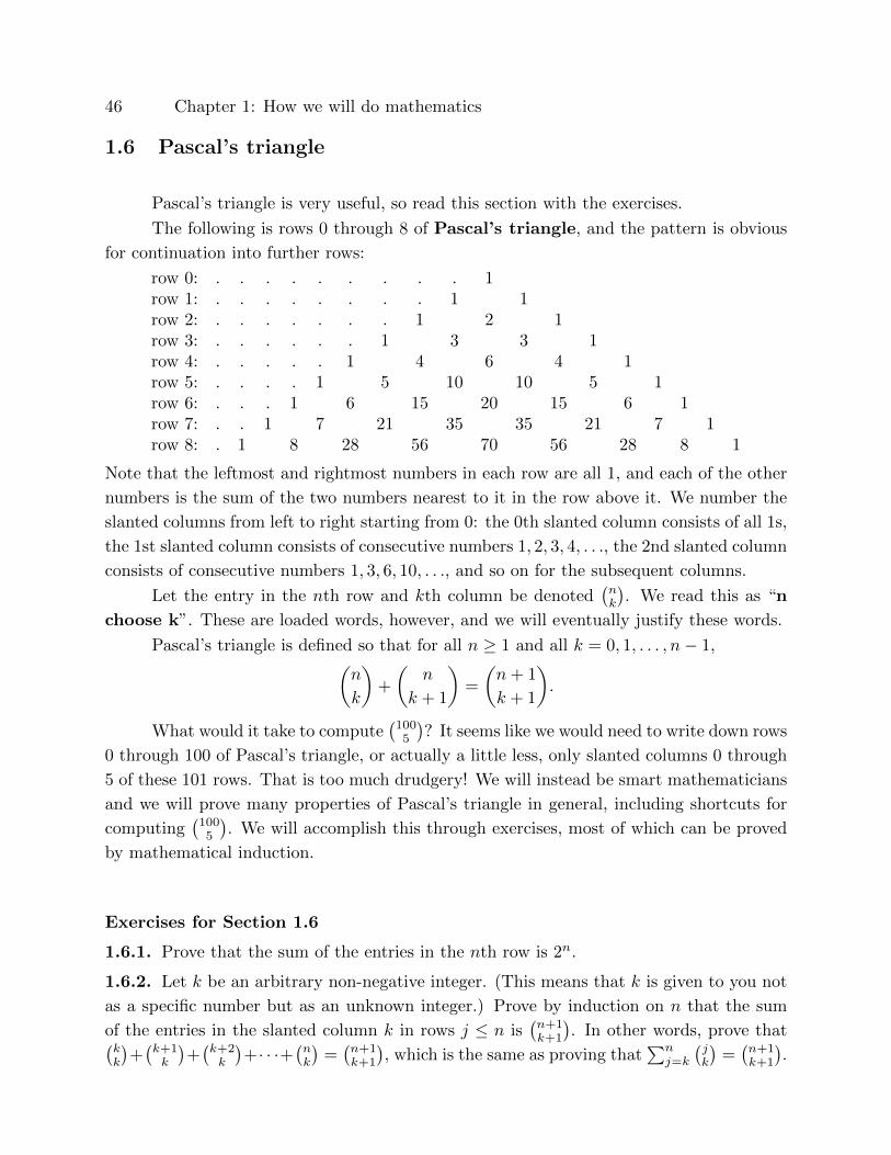
46 Chapter 1: How we will do mathematics
1.6 Pascal’s triangle
Pascal’s triangle is very useful, so read this section with the exercises.
The following is rows 0 through 8 of Pascal’s triangle, and the pattern is obvious
for continuation into further rows:
row 0: . . . . . . . . . 1row 1: . . . . . . . . 1 1row 2: . . . . . . . 1 2 1row 3: . . . . . . 1 3 3 1row 4: . . . . . 1 4 6 4 1row 5: . . . . 1 5 10 10 5 1row 6: . . . 1 6 15 20 15 6 1row 7: . . 1 7 21 35 35 21 7 1row 8: . 1 8 28 56 70 56 28 8 1
Note that the leftmost and rightmost numbers in each row are all 1, and each of the other
numbers is the sum of the two numbers nearest to it in the row above it. We number the
slanted columns from left to right starting from 0: the 0th slanted column consists of all 1s,
the 1st slanted column consists of consecutive numbers 1, 2, 3, 4, . . ., the 2nd slanted column
consists of consecutive numbers 1, 3, 6, 10, . . ., and so on for the subsequent columns.
Let the entry in the nth row and kth column be denoted(nk
). We read this as “n
choose k”. These are loaded words, however, and we will eventually justify these words.
Pascal’s triangle is defined so that for all n ≥ 1 and all k = 0, 1, . . . , n− 1,(n
k
)+
(n
k + 1
)=
(n+ 1
k + 1
).
What would it take to compute(
1005
)? It seems like we would need to write down rows
0 through 100 of Pascal’s triangle, or actually a little less, only slanted columns 0 through
5 of these 101 rows. That is too much drudgery! We will instead be smart mathematicians
and we will prove many properties of Pascal’s triangle in general, including shortcuts for
computing(
1005
). We will accomplish this through exercises, most of which can be proved
by mathematical induction.
Exercises for Section 1.6
1.6.1. Prove that the sum of the entries in the nth row is 2n.
1.6.2. Let k be an arbitrary non-negative integer. (This means that k is given to you not
as a specific number but as an unknown integer.) Prove by induction on n that the sum
of the entries in the slanted column k in rows j ≤ n is(n+1k+1
). In other words, prove that(
kk
)+(k+1k
)+(k+2k
)+· · ·+
(nk
)=(n+1k+1
), which is the same as proving that
∑nj=k
(jk
)=(n+1k+1
).

Section 1.6: Pascal’s triangle 47
1.6.3. Prove that every integer n ≥ 0 has the property that for all k = 0, 1, 2, . . . , n,(nk
)= n!
k!(n−k)! .
1.6.4. Prove that(nk
)= n(n−1)(n−2)···(n−k+1)
k! .
1.6.5. Compute(
42
),(
52
),(
62
),(
72
),(
82
),(
1002
),(
1003
),(
1004
),(
1005
).
1.6.6. Prove that(nk
)is the number of possible k-member teams in a club with exactly n
members. For this reason(nk
)is read n choose k.
†1.6.7. (This is invoked in Theorem 2.9.2, Example 8.2.9, Theorem 6.2.3.) Prove that for
all non-negative integers n,
(a+ b)n =
n∑k=0
(n
k
)akbn−k.
(Since a+ b contains two summands, it is called a binomial, and the expansion of (a+ b)n
is called the binomial expansion, with coefficients(ni
)being called by yet another name
in this context: binomial coefficients.)
1.6.8. Express each of the following as a+ b√
2 for some integers a, b:
i)√
2− 1, (√
2− 1)2, (√
2− 1)3, (√
2− 1)4, (√
2− 1)5.
ii) Write each of the five expressions in the previous part in the form√c −√d for
some positive integers c, d.
(iii)* Do you see a relation between c and d for each expression in the previous part? Is
there a general rule? Can you prove it?
1.6.9. Prove that for all positive integers n,∑nk=0(−1)k
(nk
)= 0. Compute
∑nk=0(−1)k
(nk
)in case n = 0.
1.6.10. Prove that for any non-negative integer k,
n∑j=1
j(j + 1)(j + 2) · · · (j + k) =n(n+ 1)(n+ 2) · · · (n+ k + 1)
k + 1.
(Hint: induction on n or instead use Exercises 1.6.2 and 1.6.4.)
1.6.11. Use Exercise 1.6.10 to get succinct simplifying formulas for
n∑j=1
j,n∑j=1
j(j + 1),n∑j=1
j(j + 1)(j + 2),n∑j=1
j(j + 1)(j + 2)(j + 3).
i) Note that j2 = j(j + 1) − j. Use the simplifications from above to prove that∑nj=1 j
2 = n(n+1)(2n+1)6 .
ii) From j3 = j(j + 1)(j + 2)− 3j2 − 2j = j(j + 1)(j + 2)− 3j(j + 1) + j develop the
formula for∑nj=1 j
3.
iii) Mimic the previous work to develop the formula for∑nj=1 j
4.
48 Chapter 1: How we will do mathematics
1.6.12. Prove that for all non-negative integers n and all k = 0, 1, . . . n,(nk
)≤ nk
k! .
1.6.13. Fix a positive integer k. Prove that there exists a positive number C such that
for all sufficiently large integers n, Cnk ≤(nk
).
1.6.14. Give reasons why we should have(nk
)= 0 for n < k or if either k or n is negative.
1.6.15. Let d be a positive integer. This is about summing entries in Pascal’s triangle
along the dth northwest-southeast slanted column: Prove by induction on n ≥ 0 that∑nk=0
(d+kk
)=(d+n+1n
).
*1.6.16. Prove that for all non-negative integers n,(n∑k=0
(2n
2k
)2k
)2
− 1 = 2
(n−1∑k=0
(2n
2k + 1
)2k
)2
and (n∑k=0
(2n+ 1
2k
)2k
)2
+ 1 = 2
(n−1∑k=0
(2n+ 1
2k + 1
)2k
)2
.
For notation’s sake you may want to label En =∑enk=0
(n2k
)2k and On =
∑onk=0
(n
2k+1
)2k,
where en, on are the largest integers such that 2en ≤ n and 2on + 1 ≤ n. The claim is then
that for all n ≥ 0, E22n − 1 = 2O2
2n and E22n+1 + 1 = 2O2
2n+1. (Hint: use the definition
of(nk
)to rewrite En in terms of En−1, On−1. Proceed with induction.)
Chapter 2: Concepts with which we will do mathematics
2.1 Sets
What is a set? Don’t we already have an idea of what a set is? The following formal
definition is trying to make the intuitive idea precise:
Definition 2.1.1. A set is a collection of objects. These objects are called members or
elements of that set. If m is a member of a set A, we write m ∈ A, and also say that A
contains m. If m is not a member of a set A, we write m 6∈ A.
So, while perhaps the definition does not tell us much new about what we think of
as sets, it does tell us the notation and vocabulary with which we can write and talk about
sets. For example, the set of all polygons contains triangles, squares, rectangles, pentagons,
among other polygons. The set of all polygons does not contain circles or disks. The set of
all functions contains the trigonometric, logarithmic, exponential, constant functions, and
so on.
Examples and notation 2.1.2.
(1) Intervals are sets:
(0, 1) is the interval from 0 to 1 that does not include 0, 1. From the context you
should be able to distinguish between the interval (0, 1) and a point (0, 1) in the
plane.
More generally, below we take real numbers a and b with a < b.
(a, b] is the interval from a to b that does not include a but includes b.
[a, b) is the interval from a to b that does not include b but includes a.
[a, b] is the interval from a to b that includes a and b.
(a,∞) is the interval of all real numbers strictly bigger than a.
[a,∞) is the interval of all real numbers bigger than or equal to a.
(−∞, b) is the interval of all real numbers strictly smaller than b.
(−∞, b] is the interval of all real numbers smaller than or equal to b.
(−∞,∞) is the set of all real numbers.
(0,∞) is the set of all positive real numbers.
[a, a] is the “interval” consisting of precisely one number a.
(a, a), (a, a], [a, a) are the “interval” consisting of no numbers.
(2) Descriptively we can say for example that a set A is the set of all prime numbers.
The description may be more loaded with symbols: A is the set of all real numbers x
with the property that x2 > 4x − 3. (Use the quadratic formula to prove that A
consists of the numbers that are strictly smaller than 1 or strictly larger than 3.)
50 Chapter 2: Concepts with which we will do mathematics
(3) We can list the elements and surround them with curly braces to define a set:
(i) {1, 2, 3} is the set consisting of precisely 1, 2 and 3.
(i) {1, 2, 3, 2} is the set consisting of precisely 1, 2 and 3. Thus {1, 2, 3, 2} =
{1, 2, 3}.(iii) {blue, “hello”, 5} is the set consisting precisely of the color blue, of the word
“hello”, and of number 5.
(iv) {1, 2, {1, 2}} is the set consisting of precisely of numbers 1 and 2 and of the
set {1, 2}. This set has exactly three distinct elements, it is not the same as {1, 2},and it is not the same as {{1, 2}}.
(4) The set with no elements is called the empty set and is denoted ∅ or {}.The set {∅} is not empty because it contains the empty set.
(5) When the list of elements is not small enough for reasonable explicit listing but
the pattern of elements is clear, we can start the list and then add “, . . .” when
the pattern is clear:
(i) {1, 2, 3, . . . , 10000} is the set of all positive integers that are at most 10000.
(ii) {1, 4, 9, . . . , 169} is the set of the first 13 squares of integers.
(iii) {0, 1, 2, 3, . . .} is the set consisting of all non-negative whole numbers. This
set is often denoted by N. WARNING: in some books, N stands for the set of all
positive whole numbers. To be absolutely clear, we will write N0 for {0, 1, 2, 3, . . .}and N+ for {1, 2, 3, . . .}.
(6) Warning: {3, 5, 7, . . .} or {3, 5, 7, . . . , 101} could stand for the set of all odd primes
(up to 101), or possibly for the set of all odd whole numbers strictly greater
than 1 (up to 101). Avoid ambiguities: write more elements, or write an explicit
description of the elements instead.
(7) The set of all whole numbers is written Z, the set of all rational numbers is writ-
ten Q, the set of all real numbers is written R, and the set of all complex numbers
is written C (complex numbers are defined in Section 3.9, and until then do not
worry when “C” appears in the text). The set of all non-negative real numbers
equals [0,∞), and we also write it as R≥0.
(8) We can define sets propositionally: if P is a property, then the set
{x : P (x)} or {x ∈ A : P (x)}
consists of all x (or x ∈ A) for which P holds. Here are some explicit examples:
(i) {x ∈ R : x2 = x}, and this happens to be the set {0, 1}.(ii) {x ∈ R : x > 0 and x < 1}, and this happens to be the interval (0, 1).
(iii) Q = {ab : a, b ∈ Z and b 6= 0}.(iv) {n ∈ N : n > 1 and if n = pq for some integers p, q then |p| = 1 or |q| = 1} is
the same as the set of all positive prime numbers.

Section 2.1: Sets 51
(v) A = {x : x is a positive integer that equals the sum of its proper factors}. It
is easy to verify that 1, 2, 3, 4, 5 are not in A. But 6 has factors 1, 2, 3, 6, and the
sum of the factors other than 6 equals 6. Thus 6 is an element of A. You can
verify that 28, 496, 8128 are also in A (and if you and your computer have a lot of
time, write a program to verify that no other number smaller than 33 million is in
A).
(9) Proving that a property P holds for all integers n ≥ n0 is the same as saying that
the set A = {n ∈ Z : P holds for n} contains {n0, n0 + 1, n0 + 2, . . .}. By the
principle of mathematical induction, P holds for all integers n ≥ n0 is the same as
saying that n0 ∈ A and that n− 1 ∈ A implies that n ∈ A.
Summary of example sets, and their notation
∅ = {}: the set with no elements.
{a, b, c}, {a, b, . . . , z}.{x : x can be written as a sum of three consecutive integers}.N: the set of all Natural numbers. Depending on the book, this could be the
set of all positive integers or it could be the set of all non-negative integers. The
symbols below are unambiguous:
N0: the set of all non-negative integers;
N+: the set of all positive integers.
Z: the set of all integers (“Zahlen” in German).
Q: the set of all rational numbers (Quotients).
R: the set of all Real numbers.
C: the set of all Complex numbers (more about them starting in Section 3.9).
Just like numbers, functions, and logical statements, sets and their elements can also
be related and combined in meaningful ways. The list below introduces quite a few new
concepts that may be overwhelming at first, but in a few weeks you will be very comfortable
with them.
Subsets: A set A is a subset of a set B if every element of A is an element of B. In that
case we write A ⊆ B. For example, N+ ⊆ N0 ⊆ Z ⊆ Q ⊆ R. The non-subset relation
is expressed with the symbol 6⊆: R 6⊆ N.
Every set is a subset of itself, i.e., for every set A, A ⊆ A.
The empty set is a subset of every set, i.e., for every set A, ∅ ⊆ A.
If A is a subset of B and A is not equal to B (so B contains at least one element that
is not in A), then we say that A is a proper subset of B, and we write A( B. For
example, N+ (N0 ( Z(Q(R.

52 Chapter 2: Concepts with which we will do mathematics
Equality: Two sets are equal if they consist of exactly the same elements. In other words,
A = B if and only if A ⊆ B and B ⊆ A.
Intersection: The intersection of sets A and B is the set of all objects that are in A
and in B:
A ∩B = {x : x ∈ A and x ∈ B}.
When A ∩B = ∅, we say that A and B are disjoint.
Union: The union of sets A and B is the set of all objects that are either in A or in B:
A ∪B = {x : x ∈ A or x ∈ B}.
Intersections and unions of arbitrary families of sets: We have seen intersections
and unions of two sets at a time. We can also take intersections and unions of three,
four, five, and even infinitely many sets at a time. Verify the equalities below:
(A ∩B) ∩ C = A ∩ (B ∩ C),
(A ∪B) ∪ C = A ∪ (B ∪ C),
(A ∩B) ∩ (C ∩D) = A ∩ (B ∩ C ∩D), etc
(A ∪B) ∪ (C ∪D) = (A ∪ (B ∪ C)) ∪D, etc
(Verification of the first equality above: Let x ∈ (A ∩ B) ∩ C. This holds if and only
if x ∈ A ∩B and x ∈ C, which holds if and only if x ∈ A, x ∈ B and x ∈ C, which in
turn holds if and only if x ∈ A and x ∈ (B ∩ C), i.e., if and only if x ∈ A ∩ (B ∩ C).)
Thus having established that parentheses above are irrelevant, we simply write the
four sets above as A∩B ∩C, A∪B ∪C, A∩B ∩C ∩D, A∪B ∪C ∪D, respectively.
More generally, given sets A1, A2, . . . , An, we write
n⋂k=1
Ak = A1 ∩A2 ∩ · · · ∩An = {a : a ∈ Ak for all k = 1, . . . , n},
n⋃k=1
Ak = A1 ∪A2 ∪ · · · ∪An = {a : there exists k = 1, . . . , n such that a ∈ Ak}.
The k in the subscripts are referred to as indices of unions or intersections. The indices can
be taken from arbitrary sets, even infinite ones. We call such sets index sets. Notationally,
if I is an index set, we write⋂k∈I
Ak = {a : a ∈ Ak for all k ∈ I},⋃k∈I
Ak = {a : there exists k ∈ I such that a ∈ Ak}.
Section 2.1: Sets 53
When I = {1, 2, . . . , n}, then the intersections and unioins in the two lines above are the
same as those in the previous display.
When I is the empty index set, one can argue as for empty sums in Section 1.4 that⋃k∈∅
Ak = ∅,
i.e., the empty union is that set which when unioned with any other set returns that other
set. The only set which satisfies this property is the empty set. Similarly, the empty
intersection should be that set which when intersected with any other set returns that
other set. However, this empty intersection depends on the context: when the allowed
other sets vary over all subsets of a set X, then the empty intersection equals X. We
return to this theme in Section 2.5.
Complement: The complement of A in B is
B \A = {b ∈ B : b 6∈ A}.
Some authors write B−A, but that has another meaning as well: B−A : {b− a : b ∈B and a ∈ A}. Always try to use precise and unambiguous notation.
We often have an implicit or explicit universal set that contains all elements of our
current interest. Perhaps we are talking only about real numbers, or perhaps we are
talking about all functions defined on the interval [0, 1] with values being real numbers.
In that case, for any subset A of the universal set U , the complement of A is the
complement of A in U , thus U \A, and this is denoted as Ac.
Summary notation and vocabulary
a ∈ A: a is an element of a set A.
A ⊆ B: A is a subset of set B; every element of A is an element of B.
A(B: A ⊆ B and A 6= B; A is a proper subset of B.
A = B: A ⊆ B and B ⊆ A.
A ∩B: the set of all elements that are in A and in B.
A and B are disjoint: A ∩B = ∅.A ∪B: the set of all elements that are either in A or in B.
A \B: the set of all elements of A that are not in B.
Ac: the set of all elements in the universal set that are not in A.
Example 2.1.3. We prove that Z = {3m+ 4n : m,n ∈ Z}. Certainly for any integers m
and n, 3m+ 4n is also an integer, so that {3m+ 4n : m,n ∈ Z} ⊆ Z. Now let x ∈ Z. Then
x = 1 · x = (4− 3) · x = 3(−x) + 4x,
so that x ∈ {3m + 4n : m,n ∈ Z}, whence Z ⊆ {3m + 4n : m,n ∈ Z}. Since we already
54 Chapter 2: Concepts with which we will do mathematics
proved the other inclusion, the proof is done.
Example 2.1.4. We prove that A = {6m + 14n : m,n ∈ Z} equals the set B of all even
integers. Certainly for any integers m and n, 6m+ 14n is an even integer, so that A ⊆ B.
Now let x ∈ B. Then x is even, so x = 2n for some integer n. Write
x = 2n = (14− 2 · 6)n = 6(−2n) + 14n,
so that x ∈ {6m + 14n : m,n ∈ Z} = A. Thus B ⊆ A. Together with the first part this
implies that A = B.
Example 2.1.5. The complement in Z of the set of even integers is the set of odd integers.
The complement in Q of the set of even integers contains many more elements than odd
integers. For example, it contains 12 ,
23 , . . ..
Example 2.1.6. If A ⊆ C, then C \ (C \A) = A. In other words, the complement of the
complement of A is A.
Proof. Let x ∈ A. Then x is not in the complement C ⊆ A of A in C. Since x ∈ C and not
in the subset C ⊆ A of C, it follows that x ∈ C \ (C \A). This proves that A ⊆ C \ (C \A).
Now let x ∈ C \ (C \A). Then x ∈ C and x is not in C \A. Thus necessarily x ∈ A.
This proves that C \ (C \A) ⊆ A.
Example 2.1.7. Let A and B be subsets of C. Then A ⊆ B if and only if C \B ⊆ C \A.
Proof. (⇒) Suppose that A ⊆ B. Let x ∈ C \ B. Then x ∈ C and x is not in B. Since
A ⊆ B, then necessarily x is not in B. This proves that x ∈ C ⊆ B. Since x was arbitrary
in C \B. it follows that C \B ⊆ C \A.
(⇐) Suppose that C \ B ⊆ C \ A. Then by the previous paragraph, C \ (C \ A) ⊆C \ (C \B), and so by Example 2.1.6, A ⊆ B.
Example 2.1.8. For each i ∈ N+, let Ai = [i,∞), Bi = {i, i + 1, i + 2, i + 3, . . .}, and
Ci = (−i, i). Think through the following:⋂k∈N
Ak = ∅,⋂k∈N
Bk = ∅,⋂k∈N
Ck = (−1, 1),⋃k∈N
Ak = [1,∞),⋃k∈N
Bk = N+,⋃k∈N
Ck = R.
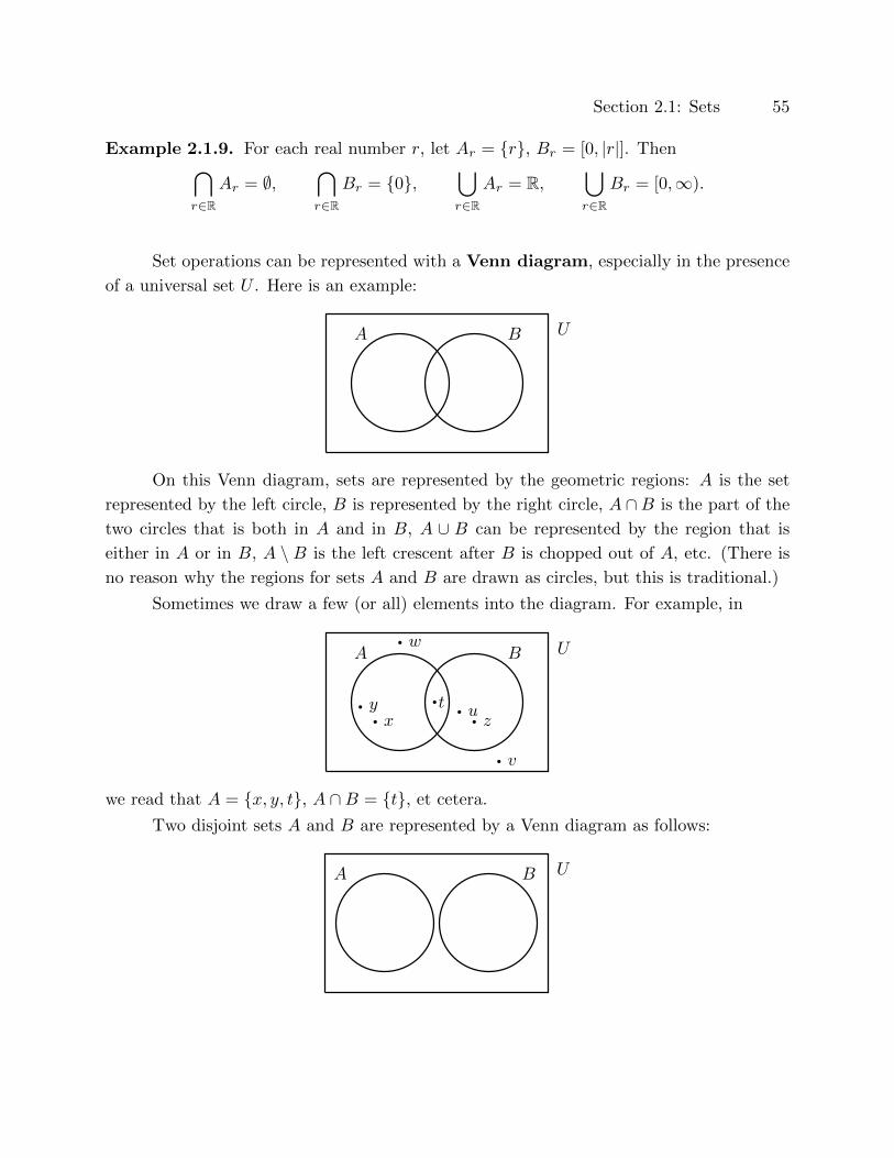
Section 2.1: Sets 55
Example 2.1.9. For each real number r, let Ar = {r}, Br = [0, |r|]. Then⋂r∈R
Ar = ∅,⋂r∈R
Br = {0},⋃r∈R
Ar = R,⋃r∈R
Br = [0,∞).
Set operations can be represented with a Venn diagram, especially in the presence
of a universal set U . Here is an example:
UA B
On this Venn diagram, sets are represented by the geometric regions: A is the set
represented by the left circle, B is represented by the right circle, A ∩B is the part of the
two circles that is both in A and in B, A ∪ B can be represented by the region that is
either in A or in B, A \ B is the left crescent after B is chopped out of A, etc. (There is
no reason why the regions for sets A and B are drawn as circles, but this is traditional.)
Sometimes we draw a few (or all) elements into the diagram. For example, in
UA B
zxy
w
u
v
t��
�
�
�
�
�
we read that A = {x, y, t}, A ∩B = {t}, et cetera.
Two disjoint sets A and B are represented by a Venn diagram as follows:
UA B
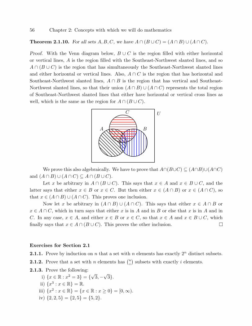
56 Chapter 2: Concepts with which we will do mathematics
Theorem 2.1.10. For all sets A,B,C, we have A ∩ (B ∪ C) = (A ∩B) ∪ (A ∩ C).
Proof. With the Venn diagram below, B ∪ C is the region filled with either horizontal
or vertical lines, A is the region filled with the Southeast-Northwest slanted lines, and so
A ∩ (B ∪ C) is the region that has simultaneously the Southeast-Northwest slanted lines
and either horizontal or vertical lines. Also, A ∩ C is the region that has horizontal and
Southeast-Northwest slanted lines, A ∩ B is the region that has vertical and Southeast-
Northwest slanted lines, so that their union (A ∩ B) ∪ (A ∩ C) represents the total region
of Southeast-Northwest slanted lines that either have horizontal or vertical cross lines as
well, which is the same as the region for A ∩ (B ∪ C).
U
A B
C
We prove this also algebraically. We have to prove that A∩(B∪C) ⊆ (A∩B)∪(A∩C)
and (A ∩B) ∪ (A ∩ C) ⊆ A ∩ (B ∪ C).
Let x be arbitrary in A ∩ (B ∪ C). This says that x ∈ A and x ∈ B ∪ C, and the
latter says that either x ∈ B or x ∈ C. But then either x ∈ (A ∩ B) or x ∈ (A ∩ C), so
that x ∈ (A ∩B) ∪ (A ∩ C). This proves one inclusion.
Now let x be arbitrary in (A ∩ B) ∪ (A ∩ C). This says that either x ∈ A ∩ B or
x ∈ A ∩ C, which in turn says that either x is in A and in B or else that x is in A and in
C. In any case, x ∈ A, and either x ∈ B or x ∈ C, so that x ∈ A and x ∈ B ∪ C, which
finally says that x ∈ A ∩ (B ∪ C). This proves the other inclusion.
Exercises for Section 2.1
2.1.1. Prove by induction on n that a set with n elements has exactly 2n distinct subsets.
2.1.2. Prove that a set with n elements has(ni
)subsets with exactly i elements.
2.1.3. Prove the following:
i) {x ∈ R : x2 = 3} = {√
3,−√
3}.ii) {x3 : x ∈ R} = R.
iii) {x2 : x ∈ R} = {x ∈ R : x ≥ 0} = [0,∞).
iv) {2, 2, 5} = {2, 5} = {5, 2}.

Section 2.1: Sets 57
v) {x ≥ 0 : x is an even prime number} = {2}.vi) ∅ is a subset of every set. Elements of ∅ are green, smart, sticky, hairy, feathery,
prime, whole, negative, positive,...
vii) {x : x can be written as a sum of three consecutive integers} = {3n : n ∈ Z}.viii) If A ⊆ B, then A ∩B = A and A ∪B = B.
2.1.4. Let U = {1, 2, 3, 4, 5, 6}, A = {1, 3, 5}, and B = {4, 5, 6}. Find the following sets:
i) (A \B) ∪ (B \A).
ii) U \ (B \A).
iii) U ∪ (B \A).
iv) U \ (A ∪B).
v) (U ∩A) ∪ (U ∩B).
vi) A \ (A \B).
vii) B \ (B \A).
viii) {A} ∩ {B}.2.1.5. Assume that A and B are disjoint subsets of U . For each part below, draw a Venn
diagram with A and B in U , and shade in the region described by the set: (i) U \ B,
(ii) A ∩ B, (iii) U \ (U \ A), (iv) (U \ A) ∩ (U \ B), (v) (U ∩ B) ∪ (U \ (B ∪ A)), (vi)
(B ∩ U) ∪ (B \ U), (vii) (U \ (U \A)) ∪B, (viii) (A ∪B) ∪ (U \A).
2.1.6. Let A,B ⊆ U .
i) Prove that there exist at most 16 distinct subsets of U obtained from A,B,U by
intersections, unions, and complementation.
ii) If A and B are disjoint, prove that there exist at most 8 such distinct subsets.
iii) If A = B, prove that there exist at most 4 such distinct subsets.
iv) If A = B = U , prove that there exist at most 2 such distinct subsets.
v) If A = B = U = ∅, prove that there exists at most 1 such subset.
2.1.7. Let A,B,C ⊆ U . Prove the following statements:
i) (A ∩ C) \B = (A \B) ∩ (C \B).
ii) (A \B) ∪ (B \A) = (A ∪B) \ (A ∩B).
iii) (A ∩B) ∪ (U \ (A ∪B)) = (U \ (A \B)) \ (B \A).
iv) U \ (A \B) = (U \A) ∪B.
v) If U = A ∩B, then A = B = U .
2.1.8. Let A,B ⊆ U .
i) Prove that (U \A)∩ (U \B) = U \ (A∪B). (The intersection of the complements
is the complement of the union.)
ii) Prove that (U \A)∪ (U \B) = U \ (A∩B). (The union of the complements is the
complement of the intersection.)
58 Chapter 2: Concepts with which we will do mathematics
2.1.9. Compute⋂k∈N+
(−1/k, 1/k),⋂k∈N+
[−1/k, 1/k],⋂k∈N+
{−1/k, 1/k}.
2.1.10. Compute⋃k∈N+
(−1/k, 1/k),⋃k∈N+
[−1/k, 1/k],⋃k∈N+
{−1/k, 1/k}.
2.2 Cartesian product
The set {a, b} is the same as the set {b, a}, as any element of either set is also the
element of the other set. Thus, the order of the listing of elements does not matter. But
sometimes we want the order to matter. We can then simply make another new notation
for ordered pairs, but in general it is not a good idea to be inventing many new notations
and concepts; it is much better if we can reuse and recycle old ones. We do this next:
Definition 2.2.1. An ordered pair (a, b) is defined as the set {{a}, {a, b}}.
So here we defined (a, b) in terms of already known constructions: (a, b) is the set one
of whose elements is the set {a} with exactly one element a, and the remaining element of
(a, b) is the set {a, b} that has exactly two elements a, b if a 6= b and has exactly one element
otherwise. Thus for example the familiar ordered pair (2, 3) really stands for {{2}, {2, 3}},(3, 2) stands for {{3}, {2, 3}}, and (2, 2) stands for {{2}, {2, 2}} = {{2}, {2}} = {{2}}.
Theorem 2.2.2. (a, b) = (c, d) if and only if a = c and b = d.
Proof. [Recall that P ⇔ Q is the same as P ⇒ Q and P ⇐ Q. Thus the proof
will consist of two parts.]
Proof of ⇒: Suppose that (a, b) = (c, d). Then by the definition of ordered pairs,
{{a}, {a, b}} = {{c}, {c, d}}. If a = b, this says that {{a}} = {{c}, {c, d}}, so that
{{c}, {c, d}} has only one element, so that {c} = {c, d}, so that c = d. But then
{{a}, {a, b}} = {{c}, {c, d}} is saying that {{a}} = {{c}}, so that {a} = {c}, so that
a = c. Furthermore, b = a = c = d, which proves the consequent in case a = b. Now
suppose that a 6= b. Then {{a}, {a, b}} = {{c}, {c, d}} has two elements, and so c 6= d.
Note that {a} is an element of {{a}, {a, b}}, hence of {{c}, {c, d}}. Thus necessarily either
{a} = {c} or {a} = {c, d}. But {a} has only one element and {c, d} has two (since c 6= d),
it follows that {a} = {c}, so that a = c. But then {a, b} = {c, d}, and since a = c, it follows
that b = d. This proves the consequent in the remaining cases.
Proof of ⇐: If a = c and b = d, then {a} = {c} and {a, b} = {c, d}, so that
{{a}, {a, b}} = {{c}, {c, d}}.Note that by our definition an ordered pair is a set of one or two sets.

Section 2.3: Relations, equivalence relations 59
Definition 2.2.3. For any sets A and B, the Cartesian product A×B of A and B is
the set {(a, b) : a ∈ A and b ∈ B} of all ordered pairs where the first component varies over
all elements of A and the second component varies over all elements of B.
In general, one can think of A×B as the “rectangle” with A on the horizontal side
and B on the perpendicular side.
Say, if A has 4 elements and B has 3 elements, then A × B can be represented by
the 12 points in the rectangle with base consisting of elements of A and height consisting
of elements of B as follows:
�
�
�
�
�
�
�
�
�
�
�
�
B
A
�
�
� � � �
�
If instead A and B are intervals as above, then A × B is the indicated rectangle.
When A and B extend infinitely far, then A × B is correspondingly a “large” rectangle:
The familiar real plane is the Cartesian product R× R.
(The three-dimensional space can be written as the Cartesian product R × (R ×R) or the Cartesian product (R × R) × R. In the former case we write elements in the
form (a, (b, c)), and in the latter case we write them in the form ((a, b), c). Those extra
parentheses are there only for notation and to slow us down, they serve no better function,
so by convention we write elements simply in the form (a, b, c).)
Exercises for Section 2.2
2.2.1. How many elements are in ∅ × R?
2.2.2. Prove that A× (B ∪ C) = (A×B) ∪ (A× C).
2.2.3. Prove that A× (B ∩ C) = (A×B) ∩ (A× C).
2.2.4. Prove that (A ∩ C)× (B ∩D) = (A×B) ∩ (C ×D).
2.2.5. Give examples of sets A,B,C,D showing that (A∪C)×(B∪D) 6= (A×B)∪(C×D).
2.2.6. Let A have m elements and B have n elements. Prove that A×B has mn elements.
Prove that A×B has 2mn subsets.

60 Chapter 2: Concepts with which we will do mathematics
2.3 Relations, equivalence relations
In this section we introduce relations in a formal way. Most relations that we even-
tually analyze will be of familiar kind, such as ≤, <, is cousin, taller than, has same birth
date, et cetera, but we can get much more structure with a formal approach.
Definition 2.3.1. A relation on A and B is any subset of A×B.
A relation on A is a relation on A and A, i.e., a subset of A×A.
We can give relation a name, such as R, and in place of “(a, b) ∈ R” we alternatively
write “aRb”. (We prefer to write “ 3 ≤ 5” rather than “(3, 5) ∈≤”.)
Examples 2.3.2.
(1) Some relations on R are ≤, <,=,≥, >. We can write (1, 2) ∈ ≤, or more familiarly,
1 ≤ 2. As a subset of R × R, ≤ consists of all points on or above the line y = x.
This relation can be drawn (and read off) easily.
(2) Draw anything in R× R. That defines a relation on R (which most likely cannot
be expressed with a formula). The relation R = {(a, b) : a, b ∈ R and a2 < b+ 1}is drawn as the set of all points (x, y) above the parabola y = x2 − 1.
(3) The following are all the possible relations on A = {1, 2} and B = {a, b}:
{(1, a), (1, b), (2, a), (2, b)},{(1, b), (2, a), (2, b)},{(1, a), (2, a), (2, b)},{(1, a), (1, b), (2, b)},{(1, a), (1, b), (2, a)},{(1, a), (1, b)},{(1, a), (2, a)},{(1, a), (2, b)},{(1, b), (2, a)},{(1, b), (2, b)},{(2, a), (2, b)},{(1, a)},{(1, b)},{(2, a)},{(2, b)},{}.

Section 2.3: Relations, equivalence relations 61
(4) A relation can be known by more than one name. Among the students in a typical
college classroom, the relations cousin and aunt are identical, i.e., no one student
is a cousin or aunt of another, so this relation equals {}, the empty relation.
Definition 2.3.3. Let R be a relation on A.
(1) R is reflexive if for all a ∈ A, aRa.
(2) R is symmetric if for all a, b ∈ A, aRb implies bRa.
(3) R is transitive if for all a, b, c ∈ A, if aRb, bRc, then aRc.
(4) R is an equivalence relation if it is reflexive, symmetric and transitive.
Examples 2.3.4.
(1) ≤ on R is reflexive and transitive but not symmetric.
(2) < on R is transitive but not reflexive or symmetric.
(3) = on any set A is reflexive, symmetric, and transitive.
(4) Being a cousin is symmetric and neither reflexive nor transitive.
(5) Being taller than is ...
(6) Let A = {u, v}. Any equivalence relation on A needs to contain (u, u) and (v, v)
in order to achieve reflexivity. The relation
{(u, u), (v, v)}
is reflexive, symmetric and transitive. The relations
{(u, u), (v, v), (u, v)} and {(u, u), (v, v), (v, u)}
are reflexive and transitive but not symmetric. The relation
{(u, u), (v, v), (u, v), (v, u)}
is an equivalence relation. Thus there are exactly two equivalence relations on A.
Definition 2.3.5. Let R be an equivalence relation on a set A. For each a ∈ A, the set
of all elements b of A such that aRb is called the equivalence class of a. We denote the
equivalence class of a with the shorthand [a].
For example, if R is the equality relation, then the equivalence class of a is {a}. If
R = A × A, then the equivalence class of any a is A. If A is the set of all students in
Math 112 this year, and aRb if students a and b are in the same section of Math 112, then
[a] is the set of all students that are in the same section as student a.
62 Chapter 2: Concepts with which we will do mathematics
Theorem 2.3.6. Let R be an equivalence relation on a set A. Two equivalence classes
are either identical or they have no elements in common.
Proof. Let a, b ∈ A, and suppose that their equivalence classes have an element in common.
Call the element c.
We now prove that the equivalence class of a is a subset of the equivalence class
of b. Let d be any element in the equivalence class of a. Then aRd, aRc and bRc imply by
symmetry that dRa and cRb, so that by transitivity dRc. Then dRc, cRb and transitivity
give dRb, so that by symmetry bRd, which says that d is in the equivalence class of b. Thus
the equivalence class of a is a subset of the equivalence class of b.
A symmetric proof shows that the equivalence class of b is a subset of the equivalence
class of a, so that the two equivalence classes are identical.
Remark 2.3.7. What this says is that whenever R is an equivalence relation on a set A,
then every element of A is in a unique equivalence class. Thus A is the disjoint union of
distinct equivalence classes. Conversely, if A = ∪i∈IAi where the Ai are pairwise disjoint,
define R ⊆ A×A as (a, b) ∈ R precisely if a and b are elements of the same Ai. Then R is
an equivalence relation: reflexivity and symmetry are obvious, and for transitivity, suppose
that a and b are in the same Ai and b and c are in the same Aj . Since Ai and Aj have the
element b in common, by the pairwise disjoint assumption necessarily i = j, so that a and
c are both in Ai. Thus R is an equivalence relation.
Example 2.3.8. Let A = {1, 2, 3, 4, 5}. The writing of A as {1, 2} ∪ {3, 4} ∪ {5} makes
the following equivalence relation on A:
{(1, 1), (1, 2), (2, 1), (2, 2), (3, 3), (3, 4), (4, 3), (4, 4), (5, 5)}.
This means is that counting all the possible equivalence relations on A is the same as
counting all the possible writings of A as unions of pairwise disjoint subsets. (In contrast,
the number of all possible relations on a set A equals the number of subsets of A×A.)
Important example 2.3.9. Let n be a positive integer. Let R be the relation on Z given
by aRb if a − b is a multiple of n. This relation is called congruence modulo n. It is
reflexive because for every a ∈ Z, a − a = 0 is an integer multiple of n. It is symmetric
because for all a, b ∈ Z, if aRb, then a−b = x ·n for some integer x, and so b−a = (−x) ·n,
and since −x is an integer, this proves that bRa. Finally, this relation R is transitive: let
a, b, c ∈ Z, and suppose that aRb and bRc. This means that a−b = x ·n and b−c = y ·n for
some integers x and y. Then a−c = a+(−b+b)−c = (a−b)+(b−c) = x·n+y·n = (x+y)·n,
and since x+y is an integer, this proves that aRc. Thus R is an equivalence relation. If aRb
for this relation R, we say that a is congruent to b modulo n, or that a is congruent
to b mod n. (Normally in the literature this is written as a ≡ bmod n.) We denote the

Section 2.3: Relations, equivalence relations 63
set of all equivalence classes with Z/nZ, and we read this as “Z mod n Z”. This set
consists of [0], [1], [2], . . . , [n − 1], [n] = [0], [n + 1] = [1], et cetera, so that Z/nZ has at
most n equivalence classes. Since any two numbers among 0, 1, . . . , n − 1 have difference
strictly between 0 and n, it follows that this difference is not an integer multiple of n, so
that [0], [1], [2], . . . , [n−1] are distinct. Thus Z/nZ has exactly n equivalence classes. Two
natural lists of representatives of equivalence classes are 0, 1, 2, . . . , n − 1 and 1, 2, . . . , n.
(But there are infinitely many other representatives as well.)
For example, modulo 12, the equivalence class of 1 is the set {1, 13, 25, 37, . . .} ∪{−11,−23,−35, . . .}, and the equivalence class of 12 is the set of all multiples of 12 (in-
cluding 0).
In everyday life we use congruence modulo 12 (or sometimes 24) for hours, modulo
12 for months, modulo 7 for days of the week, modulo 4 for seasons of the year, modulo 3
for meals of the day ...
There are exactly two equivalence classes for the congruences modulo 2: one consists
of all the even integers and the other of all the odd integers. There is exactly one equivalence
class for the congruences modulo 1: all integers are congruent modulo 1 to each other. For
the congruences modulo 0, each equivalence class consists of precisely one element.
Example 2.3.10. (Construction of Z from N0.) Consider the Cartesian product N0×N0.
Elements are pairs of the form (a, b), with a, b ∈ N0. If a, b, c, d ∈ N0, we will write
(a, b)R(c, d) if a+ d = b+ c. Thus R is a relation on N0 × N0. (Certainly you are familiar
with Z, in which case you may want to think of this relation simply saying that (a, b)R(c, d)
if a − b = c − d. The problem is that in N0 we may not be able to subtract b from a and
still get an element from N0.)
(1) R is reflexive: because for all (a, b) ∈ N0 × N0, by commutativity of addition,
a+ b = b+ a, so that by definition of R, (a, b)R(a, b).
(2) R is symmetric: if (a, b)R(c, d), then by definition a + d = b + c, so that by
commutativity of addition, d + a = c + b, and by symmetry of the = relation,
c+ b = d+ a. But by definition this says that (c, d)R(a, b).
(3) R is transitive: if (a, b)R(c, d) and (c, d)R(e, f), then by definition a + d = b + c
and c + f = d + e. It follows that (a + d) + (c + f) = (b + c) + (d + e). By
associativity and commutativity of addition, (a+ f) + (c+ d) = (b+ e) + (c+ d),
and by cancellation then a+ f = b+ e, which says that (a, b)R(e, f).
Now we define a set Z to be the set of equivalence classes for this relation. Every element
(a, b) of N0×N0 is in an equivalence class: if a ≥ b, then (a, b)R(a−b, 0), and if a < b, then
(a, b)R(0, b−a). Thus for each (a, b) ∈ N0×N0, there is an element in the equivalence class
of (a, b) of the form (0, e) or (e, 0) for some e ∈ N0, and it is left for the reader to verify that
this e is unique. In Definition 3.5.2 and beyond we identify the set of equivalence classes
64 Chapter 2: Concepts with which we will do mathematics
with the usual integers in Z as follows: the equivalence class of (e, 0) corresponds to the
non-negative integer e and the equivalence class of (0, e) corresponds to the non-positive
integer −e. In Section 3.5 we develop the arithmetic on these equivalence classes (and
hence on Z) from the arithmetic on N0.
Exercises for Section 2.3
2.3.1. Let A = {a, b} and B = {b, c, d}.i) How many elements are in the set A×A?
ii) How many elements are in the set A×B?
iii) How many elements are in the set B×B?
iv) How many relations are there on B?
v) How many relations are there on A and B? On B and A?
vi) How many relations are there on A ∪B and A ∩B?
2.3.2. Let A have n elements and B have m elements. How many distinct relations on A
and B are there? Prove.
2.3.3. In each part below, find a relation with the given properties. You may contrive a
relation on a contrived set A.
i) Reflexive, but not symmetric and not transitive.
ii) Reflexive and symmetric, but not transitive.
iii) Reflexive and transitive, but not symmetric.
iv) Symmetric, but not reflexive and not transitive.
v) Transitive, but not symmetric and not reflexive.
vi) Transitive and symmetric, but not reflexive.
2.3.4. Let A be a set with 2 elements. How many possible equivalence relations are there
on A? Repeat first for A with 3 elements, then for A with 4 elements.
2.3.5. Let A be a set with n elements. Let R be an equivalence relation on A with fewest
members. How many members are in R?
2.3.6. Let R be the relation on R given by aRb if a− b is a rational number. Prove that
R is an equivalence relation. Find at least three disjoint equivalence classes.
2.3.7. Let R be the relation on R given by aRb if a− b is an integer.
i) Prove that R is an equivalence relation.
ii) Prove that for any a ∈ R there exists b ∈ [0, 1) such that [a] = [b].

Section 2.4: Functions 65
2.3.8. Let R be a relation on R× R given by (a, b)R(c, d) if a− c and b− d are integers.
i) Prove that R is an equivalence relation.
ii) Prove that for any (a, b) ∈ R × R there exists (c, d) ∈ [0, 1) × [0, 1) such that
[(a, b)] = [(c, d)].
iii) Prove that the set of equivalence classes can be identified with [0, 1)× [0, 1).
iv) For fun: check out the video game Asteroids online for a demonstration of this
equivalence relation. Do not get addicted to the game.
2.3.9. Let A be the set of all lines in the plane.
i) Prove that the relation “is parallel to” is an equivalence relation. Note that the
equivalence class of a non-vertical line can be identified by the (same) slope of the
lines in that class. Note that the vertical lines are in their own equivalence class.
ii) Prove that the relation “is perpendicular to” is not an equivalence relation.
†2.3.10. (Invoked in Section 3.6.) For (a, b), (a′, b′) ∈ Z × Z \ {0}, define (a, b) o (a′, b′) if
a · b′ = a′ · b.i) Prove that o is an equivalence relation. (Possibly mimic Example 2.3.10.)
ii) Describe the equivalence classes of (0, 1), (1, 1), (2, 3)?
iii) Find a natural identification between the equivalence classes and elements of Q.
2.4 Functions
Here is the familiar definition of functions:
Definition 2.4.1. Let A and B be sets. A function from A to B is a rule that assigns to
each element of A a unique element of B. We express this with “f : A→ B is a function.”
The set A is the domain of f and B is the codomain of f . The range or image of f is
Image(f) = Range(f) = {b ∈ B : b = f(a) for some a ∈ A}.
But in the spirit of introducing few new notions, let’s instead define functions with
the concepts we already know. Convince yourself that the two definitions are the same:
Definition 2.4.2. Let A and B be sets. A relation f on A and B is a function if for all
a ∈ A there exists b ∈ B such that (a, b) ∈ f and if for all (a, b), (a, c) ∈ f , b = c. In this
case we say that A is the domain of f , B is the codomain of f , and we write f : A→ B.
The range of f is Range(f) = {b ∈ B : there exists a ∈ A such that (a, b) ∈ f}.
Note that this second formulation is also familiar: it gives us all elements of the
graph of the function: b = f(a) if and only if (a, b) is on the graph of f . We will freely
change between notations f(a) = b and (a, b) ∈ f .

66 Chapter 2: Concepts with which we will do mathematics
One should be aware that if f is a function, then f(x) is an element of the range and
is not by itself a function. (But often we speak loosely of f(x) being a function.)
To specify a function one needs to present its domain and its codomain, and to
show what the function does to each element of the domain.
Examples 2.4.3.
(1) A function can be given with a formula. For example, let f : R→ R be given by
f(x) = 11+x2 . The range is (0, 1]: For all x, 1 + x2 ≥ 1 with equality when x = 0.
Thus f(x) ∈ (0, 1]. For any y ∈ (0, 1], 1/y ≥ 1, so 1/y − 1 ≥ 0, so x =√
1y − 1 is
a positive real number and f(x) = y. So indeed the range of f is (0, 1].
(2) Here are formula definitions of two functions with domains [0,∞): f(x) =√x and
g(x) = −√x. Note, however, that h(x) = ±
√x is NOT a function!
(3) There may be more than one formula for a function, each of which is applied to
distinct elements of the domain. For example, define f : N+ → Z by
f(n) =
{n−1
2 , if n is odd;−n2 , if n is even.
(4) Let f : N+ → R be given by the description that f(n) equals the nth prime.
By Euclid’s theorem (proved on page 32) there are infinitely many primes so that
f is indeed defined for all positive integers. We know that f(1) = 2, f(2) = 3,
f(3) = 5, and with computer’s help I get that f(100) = 541, f(500) = 3571. There
is no algebraic formula for the nth prime.
(5) For any set A, the identity function idA : A→ A takes each x to itself.
(6) The function f : R→ R given by f(x) = 1 for all x is not the identity function.
(7) Let b ∈ B. A function f : A→ B given by f(a) = b for all a is called a constant
function.
(8) A function may be presented in a pie chart, histogram, with words, or by a table,
such as this one:
x f(x)1 12 13 2
(9) A function can be given by its graph:
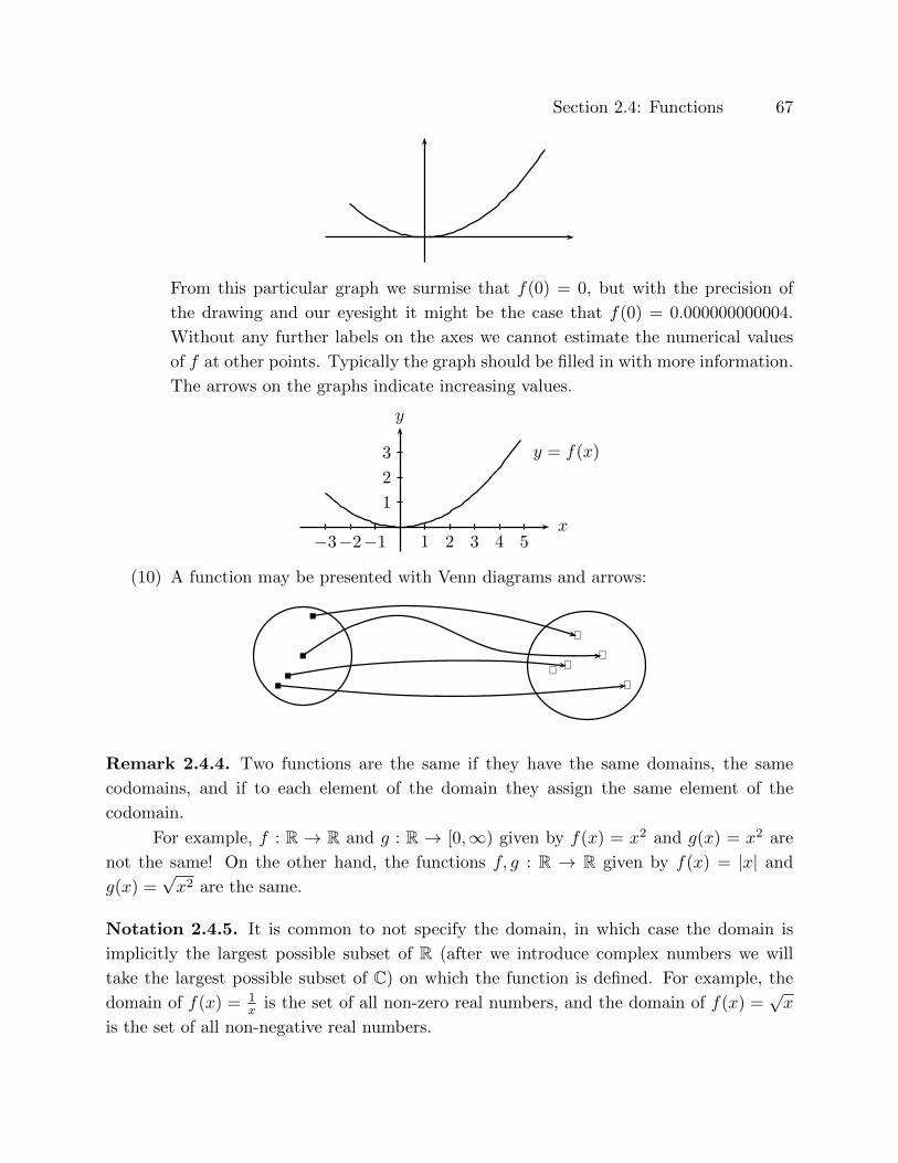
Section 2.4: Functions 67
From this particular graph we surmise that f(0) = 0, but with the precision of
the drawing and our eyesight it might be the case that f(0) = 0.000000000004.
Without any further labels on the axes we cannot estimate the numerical values
of f at other points. Typically the graph should be filled in with more information.
The arrows on the graphs indicate increasing values.
1
2
3
−3−2−1 54321x
y
y = f(x)
(10) A function may be presented with Venn diagrams and arrows:
�
�
�
�
×
××
×
×
Remark 2.4.4. Two functions are the same if they have the same domains, the same
codomains, and if to each element of the domain they assign the same element of the
codomain.
For example, f : R → R and g : R → [0,∞) given by f(x) = x2 and g(x) = x2 are
not the same! On the other hand, the functions f, g : R → R given by f(x) = |x| and
g(x) =√x2 are the same.
Notation 2.4.5. It is common to not specify the domain, in which case the domain is
implicitly the largest possible subset of R (after we introduce complex numbers we will
take the largest possible subset of C) on which the function is defined. For example, the
domain of f(x) = 1x is the set of all non-zero real numbers, and the domain of f(x) =
√x
is the set of all non-negative real numbers.

68 Chapter 2: Concepts with which we will do mathematics
Definition 2.4.6. Let A,B,C,D be sets with B ⊆ C. If f : A → B and g : C → D,
then the composition g composed with f is a function g ◦ f : A→ D such that for all
a ∈ A, (g ◦ f)(a) = g(f(a)).
If f(x) = (x+ 1)2 and g(x) = x3 − 1, then
(g ◦ f)(x) = g(f(x)) = g((x+ 1)2) = ((x+ 1)2)3 − 1 = (x+ 1)6 − 1,
(f ◦ g)(x) = f(g(x)) = f(x3 − 1) = (x3 − 1 + 1)2 = x6,
g(x)f(x) = (x3 − 1)(x+ 1)2,
and these three outcomes are distinct. For example, when plugging in x = 1, we get values
(g ◦ f)(1) = 63, (f ◦ g)(1) = 1, g(1)f(1) = 0.
Remark 2.4.7. It is common to write f2 = f ◦ f , f3 = f2 ◦ f = f ◦ f ◦ f , etc. Some
exceptions to this notation are established in trigonometry for historical reasons: “sin2(x)”
stands for “(sinx)2” and not for “sin(sinx)”. If we discovered trigonometry today, then
sin2 would have the latter meaning.
Example 2.4.8. Let f(x) =√x, and g(x) = x2. The domain of f is R≥0, and the domain
of g is R. It is possible to compose g ◦ f : R≥0 → R to obtain (g ◦ f)(x) = x, but when
composing f and g in the other order, (f ◦ g)(x) is not always equal to x. Namely, for any
negative number x, (f ◦ g)(x) = −x.
We just demonstrated that in composing two functions, the order matters.
Definition 2.4.9. A function f : A→ B is injective (or one-to-one) if for all a, a′ ∈ A,
f(a) = f(a′) implies a = a′. In other words, f is injective if whenever two things map via
f to one object, then those two things are actually the same.
A function f : A → B is surjective (or onto) if for all b ∈ B, there exists a ∈ Asuch that f(a) = b. In other words, f is surjective if every element of the codomain is
mapped onto via f by some element of the domain.
A function f : A→ B is bijective if it is injective and surjective.
For example, the identity function is bijective. The function f : R → R given by
f(x) = x2 is not injective because f(−1) = 1 = f(1). The function f : R≥0 → R given
by f(x) =√x is injective because the square root function is strictly increasing (more
about that in Section 2.9), but it is not surjective because −1 is not the square root of
any non-negative real number. The function f : R≥0 → R≥0 given by f(x) =√x is both
injective and surjective, thus bijective.
The following are all the possible functions f : {1, 2} → {1, 2} in tabular form:

Section 2.4: Functions 69
x f(x)1 12 1
x f(x)1 12 2
x f(x)1 22 1
x f(x)1 22 2
The first and the last are neither injective nor surjective, but the middle two are bijective.
The following are all the eight possible functions f : {1, 2, 3} → {1, 2} in tabular
form:
x f(x)1 12 13 1
x f(x)1 12 13 2
x f(x)1 12 23 1
x f(x)1 12 23 2
x f(x)1 22 13 1
x f(x)1 22 13 2
x f(x)1 22 23 1
x f(x)1 22 23 2
In this case no functions are injective, and all non-constant ones are surjective.
Theorem 2.4.10. The composition of two injective functions is injective.
Proof. Let f : A → B and g : C → D be injective functions, and suppose that B ⊆ C so
that we can compose the two.
If (g ◦f)(a) = (g ◦f)(a′), then g(f(a)) = g(f(a′)). Since g is injective, it follows that
f(a) = f(a′), and since f is injective, it follows that a = a′. Thus g ◦ f is injective.
Theorem 2.4.11. If f : A→ B and g : B → C are surjective functions, so is g◦f : A→ C.
If f and g are both bijective, so is g ◦ f .
Proof. Let c ∈ C. Since g is surjective, there exists b ∈ B such that g(b) = c. Since f is
surjective, there exists a ∈ A such that f(a) = b. Thus (g ◦ f)(a) = g(f(a)) = g(b) = c, so
that g ◦ f is surjective.
The last statement follows from the first part and Theorem 2.4.10.
Definition 2.4.12. We have seen polynomial functions in Section 1.4: recall that for any
subset S ⊆ R, a function f : S → R is a polynomial function if there exist a non-negative
integer n and c0, c1, . . . , cn ∈ R such that for all x ∈ S, f(x) = c0 + c1x+ c2x2 + · · ·+ cnx
n.
A function f : S → R is a rational function if there exist polynomial functions f1, f2 :
S → R such that for all x ∈ S, f2(x) 6= 0 and f(x) = f1(x)/f2(x).
Similarly there are polynomial and rational functions if all occurrences of “R” above
are replaced by “Q” or “C” .
Polynomial and rational functions are very special, and are a workhorse of analysis.
(The reader has of course encountered trigonometric, exponential, and logarithmic func-
tions, which are not polynomial or rational.) Below are some special properties. Further
special properties of polynomial functions in greater generality appear in Exercise 2.6.12.
70 Chapter 2: Concepts with which we will do mathematics
Theorem 2.4.13. If a polynomial function with real coeffiecients for now is not constant
zero, it has only finitely many roots. Specifically, if f(x) = c0 + c1x + c2x2 + · · · + cnx
n,
then the number of roots is at most n.
The domain of a rational function is the complement of a finite subset of R.
(The same statement and proof work if the coefficients are complex numbers; complex
numbers are introduced in ‘chapcomplextop’.)
Proof. At least one of ci is non-zero since f(x) is not constant 0. By possibly renaming
we may assume that cn 6= 0, and by the non-constant assumption, n ≥ 1. If n = 1, then f
has only one root, namely −c0/c1. Suppose that n ≥ 2.* In general, let a be any root of
f . By the Euclidean algorithm (Example 1.5.5), there exist polynomial functions q and r
such that
f(x) = q(x)(x− a) + r(x),
and the degree of r is strictly smaller than 1, i.e., r(x) is a constant. But if we plug x = a
into both sides, since a is a root of f , we get that r is the constant zero function, so that
f(x) = q(x)(x− a).
We write q(x) = b0 + b1x + · · · + bmxm−1. By multiplying q(x)(x − a) out we get that
m = n− 1. By induction, q(x) has at most n− 1 roots. If b is a root of f , then
0 = f(b) = q(b)(b− a),
so that either q(b) = 0 of b− a = 0. Thus b is either a root of q or b = a. Thus the roots of
f are a any any of the at most n− 1 roots of q, so that f has at most n roots. This proves
the first part.
A rational function is a quotient of two polynomial functions, and the rational func-
tion is defined everywhere except where the denominator is 0. By the first part this excludes
only finitely many numbers.
This theorem is useful in that it assures us that the domain of a rational function
contains infinitely many points, or even better, that the domain is all except finitely many
real (or complex) numbers.
* If n = 2, then by the quadratic formula the roots of c0 + c1x + c2x2 are
−c1±qc21−4c0c2
2c2. There
are root formulas for cases n = 3, 4, but executing them is very time-consuming, they require familiarity with
complex numbers, the solutions involve sums of cube roots with a few square roots thrown in for good measure,
and furthermore it can be hard to identify that the ensuing long expression simplifies to a nice root such as 2.
This, and the existence of computer capabilities, are the reasons that we do not teach such formulas. The formula
for solutions of cubic polynomials was discovered by Niccolo Fontana Tartaglia (1500–1557) and for quartic ones
by Lodovico Ferrari (1522–1565). Both formulas were popularized in a book by Gerolamo Cardano (1501–1576).
There are no formulas for general polynomials of degree n ≥ 5: not only do you and I do not know such a
formula, but Niels Henrik Abel (1802–1829) and Evariste Galois (1811–1832) proved that no formulas exist using
only radicals, sums, products, quotients.
Section 2.4: Functions 71
(You are aware that the trigonometric functions sine and cosine have infinitely many
zeroes and that tangent and cotangent are not defined at infinitely many real numbers. This
fact, together with the previous theorem, establishes that these four trigonometric functions
are not polynomial or rational functions. For similar reasons the logarithmic functions are
not polynomial or rational. We have to work harder to prove that the exponential functions
are not polynomial or rational.)
72 Chapter 2: Concepts with which we will do mathematics
Exercises for Section 2.4
2.4.1. Fix a positive integer n. Define f : Z → {0, 1, 2, 3, . . . , n − 1} by f(a) is the
remainder after a is divided by n. In number theory instead of “f(a) = b” one says a
mod n is b. We can also define a similar (but not the same!) function g : Z → Z/nZ by
g(a) = [a]. Graph the function f for n = 2 and n = 3.
2.4.2. Define the floor function b c : R → R to be the function such that for all x ∈ R,
bxc is the largest integer that is less than or equal to x. The range is Z. For example,
bπc = 3, b1c = 1, b−1.5c = −2. Graph this function.
2.4.3. The ceiling function d e : R → R is the function for which dxe is the smallest
integer that is greater than or equal to x. The range is Z. For example, dπe = 4, d1e = 1,
d−1.5e = −1. Graph this function.
2.4.4. Let A = [−a, a] or A = (−a, a), and let B be a subset of R (or of C). A function
f : A → B is an odd function (resp. even function) if for all x ∈ A, f(−x) = −f(x)
(resp. f(−x) = f(x)). Let n be a positive integer, c0, c1, . . . , cn real (or complex) numbers,
and f the polynomial function f(x) = c0 + c1x+ c2x2 + · · ·+ cnx
n.
i) Suppose that for all even k, ck = 0. Prove that f is an odd function.
ii) Suppose that for all odd k, ck = 0. Prove that f is an even function.
2.4.5. Find a set A and functions f, g : A→ A such that f ◦ g 6= g ◦ f .
2.4.6. Let h : A→ B, g : B → C, and f : C → D. Does f ◦ (g ◦h) equal (f ◦ g) ◦h? Prove
or give a counterexample.
2.4.7. Let f : R× R→ R and g : R→ R× R be given by f(x, y) = x and g(x) = (x, 0).
i) Compute f ◦ g and g ◦ f . (This means: for each function find the domain and
codomain, and show what the function evaluates to at each point in the domain.)
ii) Which among f, g, f ◦ g, g ◦ f are injective, surjective, bijective?
2.4.8. Let A = {1, 2}, B = {2, 4}, and C = {3, 6, 9}. Mark each of the following as a
function A→ B, B → C, or C → A.
i) f = {(2, 6), (4, 3)}.ii) g = {(9, 1), (6, 2), (3, 2)}.iii) h = {(1, 4), (2, 2)}.
2.4.9. For each of the following functions, state the domains, codomains, and how they
are compositions of f, g, h from the previous exercise.
i) {(2, 2), (4, 2)}.ii) {(9, 4), (3, 2), (6, 2)}.iii) {(2, 6), (1, 3)}.
Section 2.4: Functions 73
2.4.10. Let A be a set with 3 elements and B be a set with 2 elements.
i) How many possible functions are there from A to B?
ii) How many possible injective functions are there from A to B?
iii) How many possible surjective functions are there from A to B? From B to A?
iv) How many possible bijective functions are there from A to B?
v) How many possible functions from A to B are injective but not surjective?
vi) How many possible functions from A to B are surjective but not injective?
vii) How many functions from A to B are neither surjective nor injective?
2.4.11. In each part below, find f : R→ R with the specified condition.
i) f is a bijective function.
ii) f is neither injective nor surjective.
iii) f is injective, but not surjective.
iv) f is surjective, but not injective.
2.4.12. The pigeonhole principle states that if n items (such as pigeons) are put into
m holes with n > m, then at least one hole has more than one item. Let A and B be sets
with only finitely many elements.
i) Use the pigeonhole principle to demonstrate that if A has more elements than B,
then f : A→ B cannot be injective.
ii) Use the pigeonhole principle to demonstrate that if A has fewer elements than B,
then f : A→ B cannot be surjective.
iii) Use the pigeonhole principle to demonstrate that if A and B do not have the same
number of elements, then f : A→ B cannot be bijective.
2.4.13. Let A be a set with m elements and B a set with n elements.
i) How many possible functions are there from A to B?
ii) For which combinations of m,n are there injective functions from A to B?
iii) For m,n as in (ii), how many possible injective functions are there from A to B?
iv) For which combinations of m,n are there surjective functions from A to B?
v) For m,n as in (iv), how many possible surjective functions are there from A to B?
vi) For which combinations of m,n are there bijective functions from A to B?
vii) For m,n as in (vi), how many possible bijective functions are there from A to B?
2.4.14. Find an injective function f : N+ → N+ that is not surjective. Find a surjective
function g : N+ → N+ that is not injective. Compare with parts (ii) and (iv) of the previous
exercise. Does the pigeonhole principle apply?
74 Chapter 2: Concepts with which we will do mathematics
2.4.15. Let f : A→ B and g : B → C be functions.
i) Suppose that g ◦ f is injective. Prove that f is injective.
ii) Suppose that g ◦ f is surjective. Prove that g is surjective.
iii) Give an example of f, g such that g ◦ f is injective but g is not injective.
iv) Give an example of f, g such that g ◦ f is surjective but f is not surjective.
2.4.16. Find functions f, g : R→ R such that f is surjective but not injective, g is injective
but not surjective, and f ◦ g is bijective.
2.4.17. Prove that if f and g are both injective functions, then f ◦ g is also injective.
2.4.18. Prove that if f and g are both surjective functions, then f ◦ g is also surjective.
2.4.19. Prove that if f and g are both bijective functions, then f ◦ g is also bijective.
2.4.20. Suppose f : A → B. We introduce the notation f(S) = {f(x) : x ∈ S} for any
subset S of A. Let C be an arbitrary subset of A.
i) Prove f(A) \ f(C) ⊆ f(A \ C).
ii) With proof, what condition will make f(A) \ f(C) = f(A \ C)?
2.4.21. For the following polynomial and rational functions, determine the domains
(largest sets on which the function is defined):
i) f(x) = x2 − 1x3−x .
ii) f(x) = x4−2x3−1x6+2 .
(iii)* f(x) = 1x5−17x2+πx−4 . (Gottcha! We do not know the roots of this denominator.)
2.4.22. Prove that f : R→ R given by f(x) = x3 − 1 is surjective and injective.
2.4.23. Prove that the composition of polynomial functions f, g : R→ R is polynomial.
2.4.24. Prove that the composition of rational functions f, g : R→ R is rational.
2.4.25. Let f : A→ B be bijective. Prove that there exists g : B → A such that g◦f = idA
and f ◦ g = idB . Such g is called the inverse of f .
2.4.26. A function f : A → B is called invertible if there exists g : B → A such that
g ◦ f = idA and f ◦ g = idB .
i) Prove that every invertible function is bijective.
ii) Prove that g is unique, i.e., prove that if h : B → A also satisfies such that
h ◦ f = idA and f ◦ h = idB , then h = g.
2.4.27. Let f : R → R be given by f(x) = x3 − 5. Prove that f is invertible and find
its inverse. Observe that the inverse of an invertible polynomial function need not be a
polynomial function.

Section 2.5: Binary operations 75
2.4.28. (Lagrange interpolation) Let c1, . . . , cn be distinct real (or complex) numbers.
Set gj(x) =(x−c1)(x−c2)···(x−cj−1)(x−cj+1)···(x−cn)
(cj−c1)(cj−c2)···(cj−cj−1)(cj−cj+1)···(cj−cn) .
i) Prove that gj is a polynomial function and that gj(ci) =
{1, if j = i;0, otherwise.
ii) Prove that for any real (or complex) numbers d1, . . . , dn, there exists a polynomial g
of degree at most n− 1 such that for all j = 1, . . . , n, g(ci) = di.
2.4.29. When defining a function, one has to pay attention that it is well-defined. Read
through the examples below showing how a definition can go wrong.
i) The codomain is not large enough, say for f : {1, 2} → {1, 2} with f(x) = x2.
ii) The function is not defined for all elements in the specified domain, say for f : R→R that is the inverse of the squaring function or for f : R → R that returns the
multiplicative inverse.
iii) The function does not give the same answer: Let f : Z/12Z → Z be defined by
f([a]) = a. Note that f([0]) is 0, but since [0] = [12], then 0 = f([0]) = f([12]) = 12,
but the integer 0 is not equal to the integer 12.
2.4.30. Let A be the set of all differentiable functions f : R→ R. Define a relation R on
A by fRg if f(0) = g(0).
i) Prove that R is an equivalence relation.
(ii)* Let S be the set of all equivalence classes. Define F : S → R by F ([f ]) = f(0).
Prove that F is a well-defined function, in the sense that if [f ] = [g], then F ([f ]) =
F ([g]). Also prove that F is bijective.
2.4.31. Let f : N+ → Z and g : N+ → Q+ be defined by
f(n) =
{n−1
2 , if n is odd;−n2 , if n is even,
and for any positive integer with prime factorization pe11 · · · pekk let g(pe11 · · · p
ekk ) =
pf(e1)1 · · · pf(ek)
k . Assuming/knowing that prime factorization of positive integers is unique
up to order, prove that g is bijective. (We just showed that N+ and Q+ have “the same
infinite number” of elements. This proof appeared in the article Counting the rationals
by Y. Sagher, in American Mathematical Monthly 96 (1989), page 823. More people are
familiar with the proof that appears on page 266.)
76 Chapter 2: Concepts with which we will do mathematics
2.5 Binary operations
Definition 2.5.1. A binary operation on a set A is a function ◦ : A × A → A. An
arbitrary element of A × A is an ordered pair (a, b) for a, b ∈ A, and when we plug that
element into the function ◦, we should perhaps write ◦((a, b)), but normally one set of
parentheses is removed, so we write ◦(a, b). But depending on the exact form of ◦, we often
traditionally write a ◦ b rather than ◦(a, b) (see examples below).
Binary operations that we have seen are:
+,−, ·, /,×, ◦,∩,∪, or , and , xor,=⇒, ⇐⇒ .
Examples and non-examples 2.5.2.
(1) +, · on N, Z, Q, R (we of course write a + b rather than +(a, b) and a · b or even
ab rather than ·(a, b));(2) Subtraction − on Z, Q, R (but not on N);
(3) Division / on Q \ {0}, R \ {0} (but not on Q, R, N+, Z \ {0});(4) The additive inverse operation − is not a binary operation on R. (It is unary,
i.e., it acts on one number at a time.)
(5) The multiplicative inverse operation −1 is not a binary operation on R \ {0}. (It
is unary.)
(6) Let S be a set, and let A be the set of all functions f : S → S. The composition
(of functions) is a binary operation on A.
(7) ∩,∪, \ are binary operations on the set of subsets of a set S.
(8) and and or are binary operations on the set of logical statements.
Definition 2.5.3. Let ◦ be a binary operation on a set A. An element e ∈ A is an identity
element for ◦ if for all a ∈ A, a ◦ e = a = e ◦ a.
(In this chapter we use “e” for the identity element; this is a symbol that is unrelated
to the base of the exponential function as in Definition 7.6.6.)
Examples 2.5.4. An identity (or is it the identity?) for + on Z,Q,N0,R is 0. An identity
for multiplication on Z,Q,N0,R is the number 1.
An identity for composition of functions is the identity function id (the function with
id(x) = x for all x).
Subtraction on Z does not have an identity element because if e were an identity
element, then 1− e = 1 = e− 1, which says that e = 0 and e = 2, which is nonsense.
If S is a set and A is the collection of all subsets of S, then S is the identity element
for ∩ and ∅ is the identity element for ∪. The binary operation \ on A does not have an
identity unless the only element of A is the empty set.
The theorem below resolves the problem of “an identity” versus “the identity”.
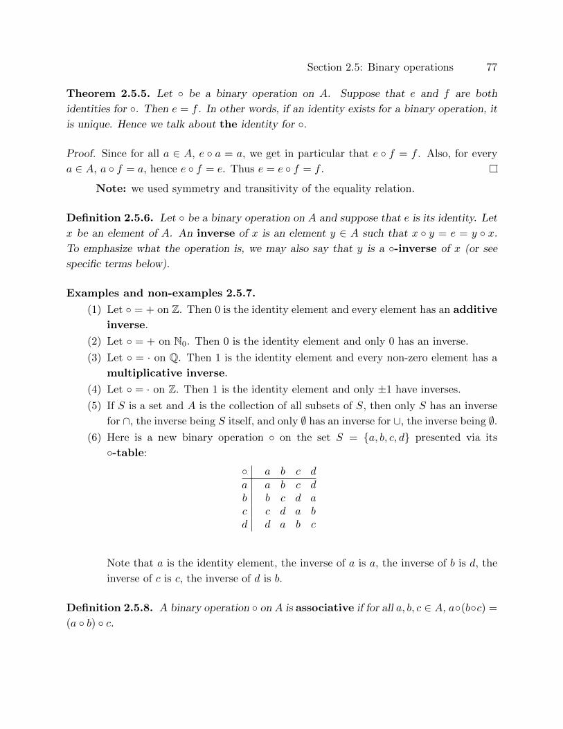
Section 2.5: Binary operations 77
Theorem 2.5.5. Let ◦ be a binary operation on A. Suppose that e and f are both
identities for ◦. Then e = f . In other words, if an identity exists for a binary operation, it
is unique. Hence we talk about the identity for ◦.
Proof. Since for all a ∈ A, e ◦ a = a, we get in particular that e ◦ f = f . Also, for every
a ∈ A, a ◦ f = a, hence e ◦ f = e. Thus e = e ◦ f = f .
Note: we used symmetry and transitivity of the equality relation.
Definition 2.5.6. Let ◦ be a binary operation on A and suppose that e is its identity. Let
x be an element of A. An inverse of x is an element y ∈ A such that x ◦ y = e = y ◦ x.
To emphasize what the operation is, we may also say that y is a ◦-inverse of x (or see
specific terms below).
Examples and non-examples 2.5.7.
(1) Let ◦ = + on Z. Then 0 is the identity element and every element has an additive
inverse.
(2) Let ◦ = + on N0. Then 0 is the identity element and only 0 has an inverse.
(3) Let ◦ = · on Q. Then 1 is the identity element and every non-zero element has a
multiplicative inverse.
(4) Let ◦ = · on Z. Then 1 is the identity element and only ±1 have inverses.
(5) If S is a set and A is the collection of all subsets of S, then only S has an inverse
for ∩, the inverse being S itself, and only ∅ has an inverse for ∪, the inverse being ∅.(6) Here is a new binary operation ◦ on the set S = {a, b, c, d} presented via its
◦-table:
◦ a b c da a b c db b c d ac c d a bd d a b c
Note that a is the identity element, the inverse of a is a, the inverse of b is d, the
inverse of c is c, the inverse of d is b.
Definition 2.5.8. A binary operation ◦ on A is associative if for all a, b, c ∈ A, a◦(b◦c) =
(a ◦ b) ◦ c.
78 Chapter 2: Concepts with which we will do mathematics
Examples and non-examples 2.5.9.
(1) + and · are associative.
(2) −, / are not associative.
(3) Composition of functions is associative. (See Exercise 2.4.6.)
(4) ∩,∪ are associative.
Theorem 2.5.10. Let ◦ be an associative binary operation on A with identity e. If x has
an inverse, that inverse is unique.
Proof. Let y and z be inverses of x. Then
y = y ◦ e (by property of identity)
= y ◦ (x ◦ z) (since z is an inverse of x)
= (y ◦ x) ◦ z (since ◦ is associative)
= e ◦ z (since y is an inverse of x)
= z (by property of identity).
Thus by the transitivity of equality, y = z.
Definition 2.5.11. We say that x is invertible if x has an inverse. The (abstract) inverse
is usually denoted x−1.
Be careful! What is the number 5−1 if ◦ equals +?
If ◦ is associative, we will in the future omit parentheses in a ◦ b ◦ c (or in a ◦ b ◦ c ◦ det cetera), as the order of the computation does not matter.
If ◦ is not associative, we need to keep parentheses! For example, in Z, a−b−c−d can
have parentheses inserted in many different ways, and four different values can be obtained.
You may want to find specific four integers a, b, c, d for which you get four distinct values
with different placements of parentheses.
Notation 2.5.12. More generally, if ◦ is associative, we may and do omit parentheses
in expressions such as a1 ◦ a2 ◦ · · · ◦ an, as the meaning is unambiguous. We abbreviate
a1 ·a2 · · · · ·an (in this order!) to∏nk=1 ak. When ◦ is addition, we abbreviate a1◦a2◦· · ·◦an
to∑nk=1 ak. Examples were already worked out in Section 1.4.
Section 2.5: Binary operations 79
Notation 2.5.13. Just like for functions in Remark 2.4.7, also for arbitrary associative
binary operation ◦ we abbreviate a ◦ a with a2, (a ◦ a) ◦ a with a3, et cetera, and in general
for all positive integers n we write
an = an−1 ◦ a = a ◦ an−1.
This notation is familiar also when ◦ equals multiplication: then 25 stands for 32. When
◦ is addition, then the abstract “25” stands for 10, but of course we prefer to not write 10
this way; instead we write it in the additive notation 2 + 2 + 2 + 2 + 2, or briefly, 5 · 2. The
empty product a0 makes sense if the set has the identity, and in that case a0 = e. (See
Exercise 1.4.6 for the first occurrence of an empty product.)
If a has a multiplicative inverse, then a−1 is that inverse, and in that case if ◦ is also
associative,
a−n = a−(n−1) ◦ a−1.
To prove this by induction on n, we multiply
(a−(n−1) ◦ a−1) ◦ an = (a−(n−1) ◦ a−1) ◦ (a ◦ an−1)
= a−(n−1) ◦ (a−1 ◦ a) ◦ an−1
= a−(n−1) ◦ an−1 = e,
and similarly an ◦ (a−(n−1) ◦ a−1) = e, which proves that a−n = a−(n−1) ◦ a−1.
Theorem 2.5.14. Let ◦ be an associative binary operation on A. Let f, g have inverses.
Then g ◦ f also has an inverse, and the inverse is f−1 ◦ g−1.
Proof. (g ◦ f) ◦ f−1 ◦ g−1 = g ◦ (f ◦ f−1) ◦ g−1 = g ◦ e ◦ g−1 = e, and similarly
f−1 ◦ g−1 ◦ (g ◦ f) = e, so that (g ◦ f)−1 = f−1 ◦ g−1.
In particular, if ◦ equals +, then for all x, y ∈ A,
−(x+ y) = (−x) + (−y),
and if ◦ equals ·, then
(x · y)−1 = y−1 · x−1.
Theorem 2.5.15. If x is invertible, then its inverse is also invertible, and the inverse of
the inverse is x.
Proof. By definition of inverses of x, x−1 ◦x = e = x◦x−1, which also reads as “the inverse
of x−1 is x.”

80 Chapter 2: Concepts with which we will do mathematics
Theorem 2.5.16. Cancellation. Let ◦ be an associative binary operation on a set A,
and z an invertible element in A. Then for all x, y ∈ A,
x ◦ z = y ◦ z ⇒ x = y,
z ◦ x = z ◦ y ⇒ x = y.
Proof. We prove only the first implication. If x◦ z = y ◦ z, then (x◦ z)◦ z−1 = (y ◦ z)◦ z−1,
hence by associativity, x ◦ (z ◦ z−1) = y ◦ (z ◦ z−1). Thus by the definition of inverses and
identities, x = x ◦ e = y ◦ e = y.
Another proof of the same fact is as follows:
x = x ◦ e= x ◦ (z ◦ z−1)
= (x ◦ z) ◦ z−1 (by associativity)
= (y ◦ z) ◦ z−1
= y ◦ (z ◦ z−1) (by associativity)
= y ◦ e= y.
Definition 2.5.17. A binary operation ◦ on A is commutative if for all a, b ∈ A, a ◦ b =
b ◦ a.
Examples and non-examples 2.5.18.
(1) +, · are commutative on all examples we have seen so far. (If you have seen
matrices, you know that matrix multiplication is not commutative.)
(2) ∩,∪ are commutative.
(3) Function composition is not commutative (cf. Example 2.4.8).
We end this section with an important example. The reader is familiar with manip-
ulations below when n = 12 or n = 24 for hours of the day (we do not say “28 o’clock”),
when n = 7 for days of the week, when n = 3 for standard meals of the day, et cetera.
Important example 2.5.19. Let n be a positive integer. Recall the definition of Z/nZfrom Example 2.3.9: elements are equivalence classes [0], [1], [2], . . . , [n − 1]. Define + on
Z/nZ as follows: [a] + [b] = [a + b]. Well, first of all, is this even a function? Namely, we
need to verify that whenever [a] = [a′] and [b] = [b′], then [a + b] = [a′ + b′], which says
that any choice of representatives gives the same final answer. Well, a− a′ and b− b′ are
integer multiples of n, hence (a+ b)− (a′+ b′) = (a−a′)+(b− b′) is a sum of two multiples
of n and hence also a multiple of n. Thus [a+ b] = [a′ + b′], which says that + is indeed a
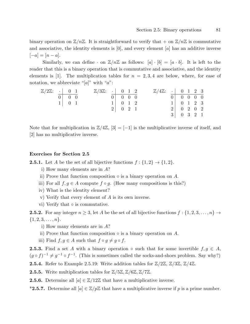
Section 2.5: Binary operations 81
binary operation on Z/nZ. It is straightforward to verify that + on Z/nZ is commutative
and associative, the identity elements is [0], and every element [a] has an additive inverse
[−a] = [n− a].
Similarly, we can define · on Z/nZ as follows: [a] · [b] = [a · b]. It is left to the
reader that this is a binary operation that is commutative and associative, and the identity
elements is [1]. The multiplication tables for n = 2, 3, 4 are below, where, for ease of
notation, we abbreviate “[a]” with “a”:
Z/2Z: · 0 10 0 01 0 1
Z/3Z: · 0 1 20 0 0 01 0 1 22 0 2 1
Z/4Z: · 0 1 2 30 0 0 0 01 0 1 2 32 0 2 0 23 0 3 2 1
Note that for multiplication in Z/4Z, [3] = [−1] is the multiplicative inverse of itself, and
[2] has no multiplicative inverse.
Exercises for Section 2.5
2.5.1. Let A be the set of all bijective functions f : {1, 2} → {1, 2}.i) How many elements are in A?
ii) Prove that function composition ◦ is a binary operation on A.
iii) For all f, g ∈ A compute f ◦ g. (How many compositions is this?)
iv) What is the identity element?
v) Verify that every element of A is its own inverse.
vi) Verify that ◦ is commutative.
2.5.2. For any integer n ≥ 3, let A be the set of all bijective functions f : {1, 2, 3, . . . , n} →{1, 2, 3, . . . , n}.
i) How many elements are in A?
ii) Prove that function composition ◦ is a binary operation on A.
iii) Find f, g ∈ A such that f ◦ g 6= g ◦ f .
2.5.3. Find a set A with a binary operation ◦ such that for some invertible f, g ∈ A,
(g ◦ f)−1 6= g−1 ◦ f−1. (This is sometimes called the socks-and-shoes problem. Say why?)
2.5.4. Refer to Example 2.5.19: Write addition tables for Z/2Z, Z/3Z, Z/4Z.
2.5.5. Write multiplication tables for Z/5Z,Z/6Z,Z/7Z.
2.5.6. Determine all [a] ∈ Z/12Z that have a multiplicative inverse.
*2.5.7. Determine all [a] ∈ Z/pZ that have a multiplicative inverse if p is a prime number.
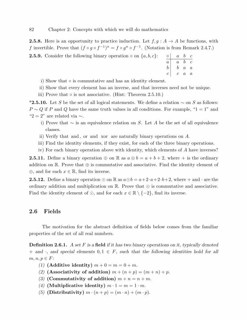
82 Chapter 2: Concepts with which we will do mathematics
2.5.8. Here is an opportunity to practice induction. Let f, g : A → A be functions, with
f invertible. Prove that (f ◦ g ◦ f−1)n = f ◦ gn ◦ f−1. (Notation is from Remark 2.4.7.)
2.5.9. Consider the following binary operation ◦ on {a, b, c}: ◦ a b ca a b cb b a ac c a a
i) Show that ◦ is commutative and has an identity element.
ii) Show that every element has an inverse, and that inverses need not be unique.
iii) Prove that ◦ is not associative. (Hint: Theorem 2.5.10.)
*2.5.10. Let S be the set of all logical statements. We define a relation ∼ on S as follows:
P ∼ Q if P and Q have the same truth values in all conditions. For example, “1 = 1” and
“2 = 2” are related via ∼.
i) Prove that ∼ is an equivalence relation on S. Let A be the set of all equivalence
classes.
ii) Verify that and , or and xor are naturally binary operations on A.
iii) Find the identity elements, if they exist, for each of the three binary operations.
iv) For each binary operation above with identity, which elements of A have inverses?
2.5.11. Define a binary operation ⊕ on R as a ⊕ b = a + b + 2, where + is the ordinary
addition on R. Prove that ⊕ is commutative and associative. Find the identity element of
⊕, and for each x ∈ R, find its inverse.
2.5.12. Define a binary operation � on R as a�b = a+2·a+2·b+2, where + and · are the
ordinary addition and multiplication on R. Prove that � is commutative and associative.
Find the identity element of �, and for each x ∈ R \ {−2}, find its inverse.
2.6 Fields
The motivation for the abstract definition of fields below comes from the familiar
properties of the set of all real numbers.
Definition 2.6.1. A set F is a field if it has two binary operations on it, typically denoted
+ and ·, and special elements 0, 1 ∈ F , such that the following identities hold for all
m,n, p ∈ F :
(1) (Additive identity) m+ 0 = m = 0 +m.
(2) (Associativity of addition) m+ (n+ p) = (m+ n) + p.
(3) (Commutativity of addition) m+ n = n+m.
(4) (Multiplicative identity) m · 1 = m = 1 ·m.
(5) (Distributivity) m · (n+ p) = (m · n) + (m · p).

Section 2.6: Fields 83
(6) (Associativity of multiplication) m · (n · p) = (m · n) · p.(7) (Commutativity of multiplication) m · n = n ·m.
(8) (Existence of additive inverses) There exists r ∈ F such thatm+r = r+m = 0.
(9) (Existence of multiplicative inverses) If m 6= 0, there exists r ∈ F such that
m · r = r ·m = 1.
(10) 1 6= 0.
0 is called the additive identity and 1 is called the multiplicative identity.
It is standard to omit “·” when no confusion arises. Note that 2 · 222 + 4 is different
from 2 222 + 4, but 2 · x+ 4 is the same as 2x+ 4.
The familiar N+, N0, Z, Q, R all have the familiar binary operations + and · on them.
Among these, N+ lacks the additive identity, but all others have the additive identity 0. In
N0, all non-zero elements lack additive inverses, and in Z, all non-zero elements other than
1 and −1 lack a multiplicative inverse. Thus N+,N0 and Z are not fields.
We take it for granted (until Chapter 3) that Q and R are fields. In Section 3.9 we
construct a new field, the field of complex numbers. There are many other fields out there,
such as the set of all real-valued rational functions with real coefficients. A few fields are
developed in the exercises to this section.
Notation 2.6.2. By Section 2.5, we know that the additive and multiplicative identities
and inverses are unique in a field. The additive inverse of m is denoted −m, and the
multiplicative inverse of a non-zero m is denoted m−1, or also 1/m. The sum n+ (−m) of
n and −m is also written as n−m, and the product n ·m−1 of n and m−1 is also written as
n/m. The latter two operations are also called subtraction and division. The functions
− and −1 are unary, with domains F and F \ {0}, respectively. By Theorem 2.5.15,
−(−m) = m, and for any non-zero m, 11m
= (m−1)−1 = m.
Another bit of notation: · takes precedence over addition, so that “(a · b) + c” can
be written simply as “a · b + c”. Note the omitting of the multiplication symbol and
the parentheses on the right but not on the left in the theorem below; if we skipped the
parentheses on the left the meaning would be different and the equality false in the given
generality.
Theorem 2.6.3. (The other distributive property) If F is a field, then for all m,n, p ∈ F ,
(m+ n)p = mp+ np.
Proof. (m+ n)p = p(m+ n) (by commutativity of multiplication)
= pm+ pn (by distributivity (5))
= mp+ np (by commutativity of multiplication).
84 Chapter 2: Concepts with which we will do mathematics
Theorem 2.6.4. If F is a field, then for all m ∈ F , m · 0 = 0 = 0 ·m.
Proof. m · 0 = m · 0 + 0 (since 0 is the additive identity).
= m · 0 + (m · 0 + (−(m · 0))) (by the definition of additive inverses)
= (m · 0 +m · 0) + (−(m · 0)) (by associativity of addition)
= m · (0 + 0) + (−(m · 0)) (by the distributive property)
= m · 0 + (−(m · 0)) (since 0 is the additive identity)
= 0 (by the definition of additive inverses).
Since multiplication is commutative, it also follows that 0 ·m = 0.
We cannot divide by 0. Never divide by 0. For one thing, in an abstract field,
dividing by 0 is simply not on the list of allowed operations, and for another, n/m always
stands for that unique element of the field, which, when multiplied by m, yields n. In other
words, n = (n/m) ·m. If m somehow – horribly – happened to be 0, then we would have
n = (n/0)·0, and by Theorem 2.6.4, this product n would be 0. So, if we were to divide by 0,
the only number that could possibly be divided by it is 0 itself. But – continuing the horrible
detour – what should 0/0 be? How about the muddle in the following usage of other axioms
that seems to require also division of 1 by 0: 0/0 = 1 ·(0/0) = (1 ·0)/0 = (0 ·1)/0 = 0 ·(1/0).
In any case, “division” by 0 is inconsistent, and not allowed. In a mathematics paper, never
write “x0 ” or “x/0”.
At this stage of your mathematical life, you will of course never write something like
“3/0” (my eyes hurt seeing this!), but a common college mistake that is essentially division
by 0 is canceling x when solving an equation such as x2 = 3x to obtain only one solution
x = 3. This cancellation was division by 0 when x was the other possible solution! Avoid
even hidden division by 0, so that you can find all the solutions.
Exercises for Section 2.6
2.6.1. Verify that the set {0} satisfies axioms (1)–(9) of fields, with 0 being the additive
and the multiplicative identity. Obviously {0} fails axiom (10).
2.6.2. Use the set-up in Example 2.3.9. Prove that Z/2Z is a field. Note that in this field
[2] = [0], so [2] does not have a multiplicative inverse. Also note that in this field, every
number has a square and cube root.
2.6.3. Use the set-up in Example 2.3.9. Prove that Z/3Z is a field. Note that in this field
[3] = [0], so [3] does not have a multiplicative inverse. Note that in this field, [2] is not the
square of any number.

Section 2.7: Order on sets, ordered fields 85
2.6.4. Use the set-up in Example 2.3.9, and let n be a positive integer strictly bigger than
1 that is not a prime integer. Prove that Z/nZ is not a field.
*2.6.5. Use the set-up in Example 2.3.9. Prove that Z/pZ is a field for any prime integer p.
Note that in Z/7Z, [2] is the square of [3] and of [4].
2.6.6. Let F be a field. Prove that (−1) · x is the additive inverse of x.
2.6.7. Let F be a field. Prove that for any x ∈ F , −(−x) = x. Prove that for any non-zero
x ∈ F , 1/(1/x) = x.
2.6.8. Let F be a field. Prove that for any x, y ∈ F , (−x) · y = −(x · y) = x · (−y). (Hint:
Use the definition of additive inverses.)
2.6.9. Let F be a field. Prove that for any x, y ∈ F , (−x) · (−y) = x · y.
2.6.10. Let x be a non-zero element of a field F . Then (−x)−1 = −(x−1).
2.6.11. Let A be a set and F a field. For any functions f, g : A → F we define new
functions f + g, f · g : F → G as (f + g)(x) = f(x) + g(x) and (f · g)(x) = f(x) · g(x).
Here, the second + and · are the binary operations on F , and the first + and · are getting
defined. Let S be the set of all functions from A to F .
i) Prove that + and · are binary operations on S.
ii) If A = F , then S includes polynomial functions. Let T be the set of all polynomial
functions from F to F . Prove that +, · and ◦ are binary operations on T .
2.6.12. (Euclidean algorithm over arbitrary fields) Let F be a field. Let f(x) = a0 +a1x+
· · ·+ anxn and g(x) = b0 + b1x+ · · ·+ bmx
m for some a0, a1, . . . , an, b0, b1, . . . , bm ∈ F and
with anbm 6= 0.
i) Suppose that m,n ≥ 1. Prove that there exist polynomials q(x) and r(x) such that
f(x) = q(x) ·g(x)+r(x) and such that the degree of r(x) is strictly smaller than m.
ii) Prove that there are at most n elements c in F such that f(c) = 0.
2.6.13. (Degree of a polynomial function) Let F be an infinite field. Let f : F → F be a
polynomial function given by f(x) = a0 +a1x+ · · ·+anxn for some non-negative integer n
and a1, a2, . . . , an ∈ F .
i) Suppose that f is the zero function. Prove that a0 = a1 = · · · = an = 0. (Hint:
Exercise 2.6.12.)
ii) Prove that the coefficients a0, a1, . . . , an are uniquely determined. In particular,
the degree of a polynomial function is uniquely determined.
2.6.14. (Degree of a polynomial function)
i) Let f, g : Z/2Z→ Z/2Z be defined by f(x) = x2, g(x) = x. Show that f and g are
an identical polynomial function given by polynomials of different degrees.
ii) Find a non-zero polynomial p(x) of degree 3 that equals the zero function on Z/2Z.
86 Chapter 2: Concepts with which we will do mathematics
2.6.15. (An unusual field.) Let ⊕ and � be binary operations on R as defined in Exer-
cises 2.5.11 and 2.5.12. Prove that R is a field with these two binary operations.
2.7 Order on sets, ordered fields
If < is a relation on a set S, we can define relations ≤, >,≥ on S by
a ≤ b means that a < b or a = b.
a > b means that b < a.
a ≥ b means that a 6< b.
Conversely, if ≤ is a relation on S, then we can define < on S by
a < b if and only if a ≤ b and a 6= b,
which by before also defines >,≥. Similarly, each of >,≥ determines all four relations of
this form. Thus one of these relations on a set S implies that we have all four relations
naturally derived from the one. These relations impose the familiar notion of orders on a
set.
We use these relations in the usual sense on R, but we can also use < in other
contexts:
Examples 2.7.1.
(1) < can be the relation “is a proper subset of” on a set S of all subsets of some uni-
versal set U . In this case, ≤ means “is a subset of”, > means “properly contains”,
and ≥ means “contains”.
(2) If < is the relation “has strictly fewer elements” on the set S of all subsets of the
set {1, 2, 3, . . . , 100}, then ≤ means “has fewer elements or is the same set” rather
than “has fewer or the same number of elements”.
Definition 2.7.2. Let ≤ be a relation on a set S.
An element b ∈ S is called an upper bound (resp. lower bound) of T (in S) if for
all t ∈ T , t ≤ b (resp. t ≥ b).*A subset T of S is bounded above (resp. bounded below) (in S) if there exists
an upper bound (resp. lower bound) of T in S.
A set that is bounded above and below is called bounded.
* A sentence of the form “P is Q (resp. Q′) if R (resp. R′)” is shorthand for two sentences: “P is Q if R”
and “P is Q′ if R′”.
Section 2.7: Order on sets, ordered fields 87
An element c ∈ S is called a least upper bound, or supremum, of T , if it is an
upper bound of T , and if for all upper bounds b of T , c ≤ b. If c ∈ T , then c is also called
the maximum of T .
An element c ∈ S is called a greatest lower bound, or infimum, of T , if it is a
lower bound of T , and if for all lower bounds b of T , b ≤ c. If c ∈ T , then c is also called
the minimum of T .
The obvious standard abbreviations are: lub(T ) = sup(T ), glb(T ) = inf(T ), max(T ),
min(T ), possibly without parentheses around T .
Examples 2.7.3.
(1) The set N0 has minimum 0. It is not bounded above, for any upper bound u
would be strictly smaller than the positive integer due + 1 (the ceiling function),
thus contradicting the assumption of upper bounds.
(2) The set T = {1/n : n ∈ N+} has maximum 1, it is bounded below, the infimum
is 0, and there is no minimum.
Proof: In long form, the set equals {1, 1/2, 1/3, 1/4, 1/5, . . .}. From this re-writing
it is clear that 1 is the maximum, that 0 is a lower bound and that 0 is not in the
set, so 0 cannot be the minimum. Why is 0 the largest lower bound, i.e., why is
0 the infimum of T? Suppose that r is a positive real number. Set n = d 1r e + 1.
Then n is a positive integer, and n > 1r . By cross multiplying we get that r > 1
n ,
which proves that r is not a lower bound on T . Since r was arbitrary, this proves
that no positive number is a lower bound on T , so that 0 is the greatest lower
bound on T .
(3) The set {1/p : p is a positive prime number} has maximum 1/2 and infimum 0.
(There are infinitely many prime numbers; see the proof on page 32.)
(4) The sets {(−1)n : n ∈ N+} and {sin(x) : x ∈ R} both have maximum 1 and
minimum −1.
(5) The set of all positive rational numbers that are strictly smaller than π has mini-
mum 0 and supremum π, but it has no maximum.
(6) The set {ex : x ∈ R} has no upper bound, it is bounded below with infimum 0,
but there is no minimum.
(7) The empty subset obviously has no minimum nor maximum. Every element of S
is vacuously an upper and a lower bound of the empty set.
(8) The set {x ∈ R : −3 < x − 5 < 3} has no minimum and maximum, but the
infimum is 2 and the supremum is 8. The set {x ∈ R : −3 ≤ x − 5 < 3} has
minimum 2, supremum 8, and no maximum. The set {x ∈ R : −3 < x − 5 ≤ 3}has maximum 8, infimum 2, and no minimum. The set {x ∈ R : −3 ≤ x− 5 ≤ 3}has minimum 2 and maximum 8.

88 Chapter 2: Concepts with which we will do mathematics
(9) If T = {{}, {1}, {2}}, then the inclusion relation on T has minimum {}, and no
upper bounds in T . If we think of T as a subset of the set S of all subsets of {1, 2}(or of the set S of all subsets of R), then T has supremum {1, 2}.
(10) If S is the set of all subsets of the set {1, 2, 3, . . . , 100} and < is the re-
lation “has strictly fewer elements”, then the empty set is the minimum
and {1, 2, 3, . . . , 100} is the maximum. If T is the subset of S consisting
only of sets with at most 2 elements, then the minimum of T is the empty
set, and there is no maximum or supremum in T . The(
1002
)elements
{1, 2}, {1, 3}, . . . , {1, 100}, {2, 3}, {2, 4}, . . . , {99, 100} are each greater than or
equal to all elements of T and they are not strictly smaller than any other element
of T .
In the sequel we restrict < to relations that satisfy the trichotomy property:
Definition 2.7.4. A relation < on a set S satisfies the trichotomy if for all s, t ∈ S,
exactly one of the following relations holds:
s = t, s < t, t < s.
Examples 2.7.5.
(1) The familiar < on R satisfies the trichotomy.
(2) If S is the set of all subsets of a universal set U , then the inclusion relation on S
satisfies the trichotomy.
(3) If S = {{}, {1}, {2}}, then the inclusion relation on S does not satisfy the tri-
chotomy.
Theorem 2.7.6. Let < on S satisfy the trichotomy. Then a supremum (resp. infimum)
of a non-empty subset T of S, if it exists, is unique.
Proof. Suppose that c, c′ are suprema of T in S. Both c and c′ are upper bounds on T , and
since c is a least upper bound, necessarily c′ ≤ c. Similarly c ≤ c′, so that by trichotomy
c = c′. This proves that suprema are unique, and a similar proof shows that infima are
unique.
Why did we assume that the subset T of S above be non-empty? By definition every
element of S is an upper bound for ∅, so in particular if S has no minimum, then ∅ has no
least upper bound.
Definition 2.7.7. A set S with relation ≤ is well-ordered if inf(T ) = min(T ) for every
non-empty subset T of S. The element min(T ) is called the least element of T .

Section 2.7: Order on sets, ordered fields 89
Examples 2.7.8.
(1) Any finite set with relation ≤ is well-ordered (simply check the finitely many
pairings for which element is smaller).
(2) Z is not well-ordered as there is no smallest whole number.
(3) Similarly, the set of all positive rational numbers is not well-ordered.
(4) N0 is well-ordered because for any non-empty subset T of N0, by the fact that
the set is not empty there exists an element n ∈ T , and after that one has to
check which of the finitely many numbers 0, 1 through n is the smallest one in T .
Similarly, N+ is well-ordered. (Chapter 3 covers this more rigorously.)
Definition 2.7.9. Let F be a set with a binary operation +, with (additive) identity
0 ∈ F , and with a relation < satisfying the trichotomy. Define F+ = {x ∈ F : 0 < x}, and
F− = {x ∈ F : x < 0}. Elements of F+ are called positive, and element of F− are called
negative. Elements of F \ F+ are called non-positive and element of F \ F− are called
non-negative.
We define intervals in F to be sets of the following form, where a, b ∈ F with a < b:
(a, b) = {x ∈ F : a < x < b},(a, b] = {x ∈ F : a < x ≤ b},[a, b) = {x ∈ F : a ≤ x < b},[a, b] = {x ∈ F : a ≤ x ≤ b},(a,∞) = {x ∈ F : a < x},[a,∞) = {x ∈ F : a ≤ x},(−∞, b) = {x ∈ F : x < b},(−∞, b] = {x ∈ F : x ≤ b}.
Definition 2.7.10. We say that a field F is an ordered field if it has a relation < with
the following properties:
(1) < satisfies the trichotomy, i.e., for all x, y ∈ F , exactly one of the following is true:
x < y, x = y, y < x.
(2) (Transitivity of <) For all x, y, z ∈ F , if x < y and y < z then x < z.
(3) (Compatibility of < with addition) For all x, y, z ∈ F , if x < y then x+ z <
y + z.
(4) (Compatibility of < with multiplication by positive elements) For all
x, y, z ∈ F , if x < y and 0 < z then xz < yz.
A subset of an ordered field is called an ordered set.
90 Chapter 2: Concepts with which we will do mathematics
It follows that Q is an ordered field as well: it is a field, and the trichotomy, transitiv-
ity, and compatibilities of < hold on Q as they hold on the larger set R. These properties
of < also hold on the subsets N+,N0 and Z, even if the latter sets are not fields.
Theorem 2.7.11. Let F be an ordered set.
(1) For x ∈ F with the additive inverse −x ∈ F , x ∈ F+ if and only if −x ∈ F−, and
x ∈ F− if and only if −x ∈ F+.
(2) 1 ∈ F+.
(3) For x ∈ F with the multiplicative inverse x−1 ∈ F , x ∈ F+ if and only if x−1 ∈ F+,
and x ∈ F− if and only if x−1 ∈ F−.
Proof. (1) x ∈ F+ if and only if 0 < x, and by compatibility of < with addition this implies
that −x = 0− x < x− x = 0, so that −x ∈ F−. The rest of (1) is equally easy.
(2) By assumption 1 6= 0. If 1 6∈ F+, then by trichotomy 1 < 0, and by (1), 0 < −1.
Thus by compatibility of < with multiplication by positive numbers, since −1 is supposedly
positive, 0 = 0 ·(−1) < (−1) ·(−1). By Exercise 2.6.9, (−1) ·(−1) = 1, which by transitivity
says that 0 < 1. Since we also assumed that 1 < 0, we get a contradiction to the trichotomy.
So necessarily 1 ∈ F+.
(3) Suppose that x ∈ F+. By trichotomy then exactly one of the following three
inequalities holds: x−1 < 0, x = 0, x−1 > 0. Let stand for the correct inequality (or
equality). By compatibility of < with multiplication by the positive number x, we then
have 1 = x · x−1 x · 0 = 0. By (2), the relation must equal >, so that x−1 > 0.
If instead x ∈ F−, then by (1), −x ∈ F+, and by what we have proved of (3),
(−x)−1 ∈ F+. By Exercise 2.6.10 then −x−1 = (−x)−1 ∈ F+, so that x−1 ∈ F− by (1).
Theorem 2.7.12. Let F be an ordered field.
(1) For x, y ∈ F+, x+ y is also in F+.
(2) For x, y ∈ F+, x · y is also in F+.
(3) For x, y ∈ F−, x+ y ∈ F−.
(4) For x, y ∈ F−, x · y ∈ F+.
(5) For x ∈ F+ and y ∈ F−, x · y ∈ F−.
Proof. (1) By assumption, 0 < x and 0 < y. Then by compatibility of < with addition,
y = 0 + y < x+ y, and since 0 < y, by transitivity of <, 0 < x+ y, i.e., x+ y ∈ F+.
(2) By assumption, 0 < x and 0 < y. Then by compatibility of < with multiplication
by positive numbers, 0 = 0 · y < x · y, which proves that x · y ∈ F+.
The proofs of the rest are similar.
Exercises for Section 2.7
Section 2.7: Order on sets, ordered fields 91
2.7.1. Prove that if < is transitive then ≤ is transitive.
2.7.2. Prove that < (resp. ≤) is transitive if and only if > (resp. ≥) is transitive.
2.7.3. (An exercise of this flavor is relevant in computing limits as in Section 4.1.) Under
what conditions is the minimum of {0.2, ε/7} equal to 0.2, and when is the minimum ε/7?
Similarly determine min{0.2, ε/7, ε2/4}.2.7.4. For each of the subsets of R below, determine its minimum, maximum, infimum,
supremum, if applicable. Justify all answers.
i) {−1, 2, π,−7}.ii) {(−1)n/n : n ∈ N+}.iii) The set of all positive prime numbers.
iv) {x ∈ R : −1 < x < 5}.v) {x ∈ R : 2 ≤ x < 5}.
vi) {x ∈ Q : x2 < 2}.vii) {x ∈ R : x2 + x− 1 = 0}.viii) {x ∈ Q : x2 + x− 1 = 0}.ix) {n/(n+ 1) : n ∈ N0}.
2.7.5. Suppose that a subset T of an ordered field has a minimum (resp., maximum,
infimum, supremum) b. Prove that the set −T = {−t : t ∈ T} has a maximum (resp.,
minimum, supremum, infimum) −b.2.7.6. Suppose that a subset T of positive elements of an ordered field has a minimum
(resp., maximum, infimum, supremum) b. What can you say about the maximum (resp.,
minimum, supremum, infimum) of the set {1/t : t ∈ T}?†2.7.7. (Invoked in Theorem 7.3.4.) Let S and T be subsets of an ordered field F . Let
S + T = {s+ t : s ∈ S and t ∈ T}.i) If S and T are bounded above, prove that sup(S + T ) ≤ supS + supT .
ii) If S and T are bounded below, prove that inf(S + T ) ≥ inf S + inf T .
2.7.8. Let F be an ordered field. Prove that 2, 3 are positive (and so not zero).
2.7.9. Let F be a field and x ∈ F . Prove that x2 = 0 if and only if x = 0.
2.7.10. Let F be an ordered field and x ∈ F . Let x, y ∈ F be non-negative (resp. non-
positive) such that x+ y = 0. Prove that x = y = 0.
2.7.11. Let F be an ordered field. Suppose that x ≤ y and p ≤ q. Prove that x+p ≤ y+q.
If in addition x < y or p < q, prove that x+ p < y + q.
2.7.12. Let F be an ordered field and x, y ∈ F . Prove that x < y if and only if 0 < y− x.
Prove that x ≤ y if and only if 0 ≤ y − x.
2.7.13. Let F be an ordered field, and x, y ∈ F+ with x < y. Prove that 1/y < 1/x.
92 Chapter 2: Concepts with which we will do mathematics
2.7.14. Let F be an ordered field. Suppose that x < y and that x, y are non-zero. Does
it follow that 1/y < 1/x? Prove or give a counterexample.
†2.7.15. (In-betweenness in an ordered field) Let F be an ordered field. Let x, y ∈ F with
x < y. Prove that x < (x+ y)/2 < y. (Why are we allowed to divide by 2?)
2.7.16. Find an ordered set without a minimum.
2.7.17. Let F be an ordered set. Prove that any non-empty finite subset S of F has a
maximum and a minimum. Prove that for all s ∈ S, min(S) ≤ s ≤ max(S).
2.7.18. Let n > 1 be an integer and F = Z/nZ. (This was defined in Example 2.3.9.)
Prove that F is not an ordered set. In particular, using Exercise 2.6.5, for any prime
integer p, Z/pZ is a field that is not ordered.
2.8 What are the integers and the rational numbers?
Rational numbers and integers are very special real numbers, and non-negative inte-
gers are more special still. This section contains a formal definition of N0 as a subset of Rwith derivations of a few important properties.
The set Z of all integers is defined as N0 ∪ {n ∈ R : −n ∈ N0}; The set Q of all
rational numbers is defined as {x ·y−1 : x ∈ Z, y ∈ N+}. In this section we derive no special
properties of Z or of Q. (We all have an intuitive notion what these numbers are, and in
order to get to the formal power series at the end of this book in reasonable amount of time
I recommend covering this section very lightly if at all. Construction of N0 independent
of R is done formally in the next chapter, and we also derive there all the properties from
this section. Regardless of whether you read this section or not, you should be able to do
any exercises here.)
We use Theorem 3.8.2 saying that R is an ordered field.
Definition 2.8.1. A subset T of R is called inductive if 0 ∈ T and if for every element
n of T , n+ 1 is also in T .
Examples of inductive sets are R and R+ ∪ {0}.
Theorem 2.8.2. There exists an inductive subset N0 of R that is a subset of every induc-
tive subset of R.
(1) N0 is the smallest inductive subset of R.
(2) If m ∈ N0 is non-zero, then m = n+ 1 for some n ∈ N0.
(3) All elements of N0 \ {0} are positive.

Section 2.8: What are the integers and the rational numbers? 93
Proof. We know that the collection S of inductive subsets of R is a non-empty set. We
define N0 as the intersection of all sets in S. Since 0 is in every inductive set, then 0 is
also in their intersection N0. If n ∈ N0, then n is in every inductive subset of R, and so
by the definition of inductive sets, n + 1 is in every inductive subset of R, and so it is in
their intersection N0. This proves that N0 is an inductive set. By definition it is a subset
of every inductive subset of R. This proves (1).
Suppose that m ∈ N0 is not 0 and is not equal to n + 1 for any n ∈ N0. Let
T = N0 \ {m}. Then 0 ∈ T , and if n ∈ T , then n + 1 ∈ T , so that T is an inductive set.
But N0 is a subset of every inductive set, so that m ∈ N0 would have to be in T , which is a
contradiction. Thus every non-zero m ∈ N0 equals n+ 1 for some n ∈ N0. This proves (2).
Let T = N0 \ R−. Then 0 ∈ T . If n ∈ T , then by trichotomy, n = 0 or n ∈ R+, and
hence n+ 1 ∈ R+ ∩ T . Since T is inductive. This proves (3).
Theorem 2.8.3. Let n ∈ N0. There are no elements of N strictly between n and n+ 1.
Proof. Let T be the subset of N0 consisting of all n that satisfy the property that there
are no elements of N strictly between n and n + 1. Suppose that there exists m ∈ N0
strictly between 0 and 0 + 1 = 1. Then by Theorem 3.1.7, m = p+ 1 for some p ∈ N0. By
compatibility of order with addition, p = m− 1 < 1− 1 = 0, contradicting Theorem 2.8.2
which asserts that elements of N0 are non-negative. This proves that 0 ∈ T .
Now suppose that n ∈ T . We want to prove that n+1 ∈ T . Suppose for contradiction
that there exists m ∈ N0 that is strictly between n+1 and (n+1)+1. Since m > n+1 ≥ 1,
m is not zero, so that by Theorem 3.1.7, m = p+1 for some p ∈ N0. Then by compatibility
of order with addition, p is strictly between n and n+ 1, which contradicts the assumption
that n ∈ T . So necessarily there is no m with the stated property, so that n+ 1 ∈ T .
This proves that T is an inductive subset of N0, and since N0 is contained in every
inductive subset, the theorem is proved.
Theorem 2.8.4. If n,m ∈ N0 and n ≤ m, then m− n ∈ N0.
Proof. Let T = {n ∈ N0 : if m ∈ N0 and n ≤ m, then m− n ∈ N0. We will prove that T
is an inductive set. Certainly 0 ∈ T as m − 0 = m. Now suppose that n ∈ T . We claim
that n + 1 ∈ T . Namely, let m ∈ N0 such that n + 1 ≤ m. Necessarily 1 ≤ m so that by
Theorem 3.1.7, m = p+1 for some p ∈ N0. By compatibility of ≤ with addition then n ≤ p,and since n ∈ T , it follows that p−n ∈ N0. Hence m−(n+1) = p+1−(n+1) = p−n ∈ N0.
This proves that n+1 ∈ T . Since n was arbitrary, this proves that T is an inductive subset
of N0, and since N0 is a subset of every inductive set we have that T = N0. This proves
the theorem.
94 Chapter 2: Concepts with which we will do mathematics
Theorem 2.8.5. (The well-ordering principle) N0 is well-ordered (see Definition 2.7.7).
In other words, every non-empty subset S of N0 has a least element, that is, S contains
an element r such that for all t ∈ S, r ≤ t.
Proof. We will prove that the following set is inductive:
T = {n ∈ N0 : if S ⊆ N0 and n ∈ S, then S has a least element}.
Note that 0 ∈ T because 0 ≤ n for all n ∈ N0 and hence 0 ≤ n for all n ∈ S.
Suppose that n ∈ T . We next prove that n+ 1 ∈ T . Let S ⊆ N0 and n+ 1 ∈ S. By
assumption that n ∈ T , it follows that the set S∪{n} has a least element. Thus there exists
r ∈ S ∪ {n} such that for all t ∈ S, r ≤ t and r ≤ n. If r ∈ S, then we just showed that
for all t ∈ s, r ≤ t, so that S has a least element. Now suppose that r 6∈ S. So necessarily
r = n, and this is not an element of S. Then we claim that n + 1 is the least element of
S. Namely, let t ∈ S. We need to prove that n + 1 ≤ t. Suppose for contradiction that
t < n + 1. Since n is the least element of S ∪ {n}, it follows that n ≤ t. Thus we have
n ≤ t < n + 1, so that by Theorem 3.1.8, necessarily n = t. But then n = t ∈ S, which
contradicts the assumption that n 6∈ S. Thus n + 1 ≤ t, and since t was an arbitrary
element of S, it follows that n+ 1 is the least element of S. Thus in all cases, if n+ 1 ∈ S,
the set S has a least element. So n + 1 ∈ T . Thus T is an inductive set, and hence equal
to N0. This means that every non-empty subset of N0 has a least element.
Exercises for Section 2.8
You should be able to do these problems without reading this section.
2.8.1. Let F be an ordered field and let x ∈ F satisfy x > 1. Prove that for all positive
integers n, xn > 1 and xn+1 > x.
2.8.2. Let F be an ordered field and let x ∈ F satisfy 0 < x < 1. Prove that for all
positive integers n, 0 < xn < 1 and xn+1 < x.
2.8.3. (Bernoulli’s inequality) Prove that for all x ∈ R≥0 and all n ∈ N0, (1 + x)n ≥1 + nx.
2.8.4. Does the set {2n/n : n ∈ N+} have a lower (resp. upper bound)? Is it well-ordered?
Justify. Repeat with {n/2n : n ∈ N+}.2.8.5. Prove that for all n ∈ Z there exist no integer strictly between n and n + 1.
(Hint: if n is negative, then the interval (n, n+ 1) can be mirrored across 0 to the interval
(−n− 1, (−n− 1) + 1).)
2.8.6. Prove that for all x ∈ R, the interval (x, x+ 1) can contain at most one integer.
Section 2.9: Increasing and decreasing functions 95
2.9 Increasing and decreasing functions
Definition 2.9.1. Let F,G be ordered sets (as in the previous section), and let A ⊆ F .
A function f : F → G is increasing (resp. decreasing) on A if for all x, y ∈ A, x < y
implies that f(x) ≤ f(y) (resp. f(x) ≥ f(y)). If furthermore f(x) < f(y) (resp. f(x) > f(y)
for all x < y, then we say that f is strictly increasing (resp. strictly decreasing) on A.
A function is (strictly) monotone if it is (strictly) increasing or (strictly) decreasing.
Theorem 2.9.2. Let n be a positive integer and F an ordered field. Then the function
f : F → F defined by f(x) = xn is strictly increasing on F+ ∪ {0}.
Proof. Let x, y ∈ F+ ∪ {0} with x < y. Then by Exercise 1.6.7,
f(y)− f(x) = yn − xn
= (x+ (y − x))n − xn
=
n∑k=0
(n
k
)xk(y − x)n−k − xn
=
n−1∑k=0
(n
k
)xk(y − x)n−k = (y − x)n +
n−1∑k=1
(n
k
)xk(y − x)n−k.
Since y−x is positive, by Theorem 2.7.12, (y−x)n is also positive. Since in addition x ≥ 0
and(nk
)is a non-negative integer, then by the compatibilities of >,
∑n−1k=1
(nk
)xk(y−x)n−k ≥
0. Thus f(y)− f(x) > 0.
Corollary 2.9.3. Let n be a positive integer and F an ordered field. Suppose that x, y ∈F+ ∪ {0} have the property that xn < yn. Then x < y. (In other words, the nth radical
function is strictly increasing on F+ ∪ {0}.)
Proof. If x = y, then xn = yn, which contradicts the assumption and trichotomy. If x > y,
then by Theorem 2.9.2, xn > yn, which also contradicts the assumption. So by trichotomy
x < y.
Theorem 2.9.4. If F,G are ordered sets and f : F → G is strictly monotone, then f is
injective, and there exists a strictly monotone function g : Range(f)→ F such that for all
x ∈ F , (g ◦ f)(x) = x and for all y ∈ G, (f ◦ g)(y) = y. In other words, g is the inverse of
the function f : F → Range(f).
Proof. Let y ∈ Range(f). Then y = f(x) for some x ∈ F . If also y = f(z) for some z ∈ F ,
since f is strictly monotone, x = z. So f is injective and x is unique. Thus we define
g : Range(f) → F by g(y) = x. Then by definition for all x ∈ F , g(f(x)) = x and for all
y ∈ Range(f), f(g(y)) = y. If f is increasing and y1, y2 ∈ Range(f) such that y1 < y2, then
96 Chapter 2: Concepts with which we will do mathematics
g(y1) < g(y2) for otherwise by the increasing property of f , y1 = f(g(y1)) ≥ f(g(y2)) = y2,
which is a contradiction. Thus if f is increasing, so is g = f−1. Thus if g = f−1 is
increasing, so is f = (f−1)−1. The same reasoning goes for the decreasing property.
Remark 2.9.5. Let F be an ordered set and G an ordered field. Let f, g : F → G
be functions. Below we need the definitions of the sum and product of functions (see
Exercise 2.6.11).
(1) If f, g are both strictly increasing (resp. both decreasing), then f + g is strictly
increasing (resp. decreasing).
(2) If f, g are both strictly increasing (resp. both decreasing) and always take on
positive values, then fg is strictly increasing (resp. decreasing).
(3) If f, g are both strictly increasing (resp. both decreasing) and always take on
negative values, then fg is strictly decreasing (resp. increasing).
Proof of (3): Let x, y ∈ F with x < y. Suppose that f and g are both increas-
ing functions, so that f(x) < f(y) < 0 and g(x) < g(y) < 0. Then −f(y), −g(x)
are positive numbers, so by compatibility of < with multiplication by positive numbers,
f(x)(−g(x)) < f(y)(−g(x)) and (−f(y))g(x) < (−f(y))g(y). By Exercise 2.6.8, this
says that −(f(x)g(x)) < −(f(y)g(x)) and −(f(y)g(x)) < −(f(y))g(y)). By transitiv-
ity of < then −(f(x)g(x)) < −(f(y))g(y)). By compatibility of < with addition, by
adding f(x)g(x) + f(y)g(y) we get that f(y)g(y) < f(x)g(x). With function notation,
(fg)(y) < (fg)(x), and since x and y were arbitrary, this says that fg is strictly decreas-
ing. The proof in the case where both f and g are strictly decreasing is similar.
Exercises for Section 2.9
2.9.1. Let n be an odd positive integer and F an ordered field. Prove that the function
f : F → F defined by f(x) = xn is strictly increasing.
2.9.2. Let n be an even positive integer and F an ordered field. Prove that the function
f : F− ∪ {0} → F defined by f(x) = xn is strictly decreasing.
2.9.3. Let n be an odd positive integer and F an ordered field. Suppose that a, b ∈ F and
that an < bn. Prove that a < b.
2.9.4. Let F be an ordered field, a ∈ F+ and f : F → F defined by f(x) = ax. Prove
that f is a strictly increasing function.
2.9.5. Let F be an ordered field, a ∈ F− and f : F → F defined by f(x) = ax. Prove
that f is a strictly decreasing function.
Section 2.10: Absolute values 97
2.9.6. Prove that the composition of (strictly) increasing functions is (strictly) increasing.
Prove that the composition of (strictly) decreasing functions is (strictly) increasing.
2.9.7. Prove that the composition of a (strictly) increasing function with a (strictly) de-
creasing function, in any order, is (strictly) decreasing.
2.9.8. Suppose that f : F → G is strictly monotone.
i) Let B be a subset of F , and define g : B → G by g(x) = f(x). Prove that g is
strictly monotone.
ii) Define h : B → Range(g) by h(x) = f(x). Prove that h is bijective.
2.9.9. Give an example of a non-decreasing function f : R→ R that is not injective.
2.10 Absolute values
Definition 2.10.1. Let F be an ordered field. The absolute value function | | : F → F
is a function defined as
|x| =
{0; if x = 0;x; if x ∈ F+;−x; if x ∈ F−.
This defines the absolute value function on the ordered fields Q and R.
The following theorem lists the familiar properties of absolute values, and the reader
may wish to prove them without reading the given proof.
Theorem 2.10.2. Let F be an ordered field.
(1) For all x ∈ F , |x| ≥ 0. Furthermore, x ≥ 0 if and only if x = |x|; and x ≤ 0 if and
only if x = −|x|. (In particular, |1| = 1.)
(2) For all x ∈ F , |x| = | − x|.(3) For all x ∈ F , −|x| ≤ x ≤ |x|.(4) For all x, a ∈ F , |x| ≤ a if and only if −a ≤ x ≤ a.
(5) For all x, a ∈ F , |x| < a if and only if −a < x < a.
(6) For all x, y ∈ F , |xy| = |x||y|.
Proof. (1) is from the definition.
(2) Certainly |0| = | − 0| = 0. Suppose that x ∈ F−. Then |x| = −x and −x ∈ F+
so that | − x| = −x. Thus |x| = −x = | − x|. If x ∈ F+, then −x ∈ F−, so that by what
we just proved, | − x| = | − (−x)| = |x|.(3) If x ≥ 0, then |x| = x, and if x < 0, then x < 0 < |x|. Thus by transitivity for
all x, x ≤ |x|. In particular, when applied to −x, this says that −x ≤ | − x| = |x|, and by
adding x− |x| to both sides we get that −|x| ≤ x.
(4) Suppose that |x| ≤ a. Then by (3) and transitivity, x ≤ a, and −x ≤ | − x| =
|x| ≤ a, so that by transitivity and adding x− a to both sides, −a ≤ x.
98 Chapter 2: Concepts with which we will do mathematics
(5) The proof of (5) is similar to that of (4).
(6) We may choose r and s ∈ {1,−1} such that rx ≥ 0 and sy ≥ 0. Then
|xy| = | ± (xy)| (by (2))
= |(rx)(sy)|= (rx)(sy) (by Theorem 2.7.12)
= |rx| · |sy| (by the definition of r, s)
= |x||y| (by (2)).
In the next theorem we use the standard notation “±” when we mean that the result
should hold in place either for + or for −.
Theorem 2.10.3. The following inequalities hold for an ordered field F .
(1) Triangle inequality: For all x, y ∈ F , |x± y| ≤ |x|+ |y|.(2) Reverse triangle inequality: For all x, y ∈ F , |x± y| ≥ ||x| − |y|| = ||y| − |x||.
Proof. (1) By the first part of the previous theorem, −|x| ≤ x ≤ |x| and −|y| ≤ y ≤ |y|.Thus
−(|x|+ |y|) = (−|x|) + (−|y|) (by Theorem 2.5.14)
≤ x+ (−|y|) (by compatibility of ≤ with addition)
≤ x+ y (by compatibility of ≤ with addition)
≤ |x|+ y (by compatibility of ≤ with addition)
≤ |x|+ |y| (by compatibility of ≤ with addition),
so that by transitivity, −(|x| + |y|) ≤ x + y ≤ |x| + |y|. Thus by part (4) of the previous
theorem, |x+ y| ≤ |x|+ |y|. It follows that |x− y| = |x+ (−y)| ≤ |x|+ | − y|, and by the
second part again this is equal to |x|+ |y|.(2) By (1), |x| = |x ± y − ±y| ≤ |x ± y| + |y|, so that |x| − |y| ≤ |x ± y|. Similarly,
|y| − |x| ≤ |y± x|. But by the second part of the previous theorem, |y− x| = | − (y− x)| =|x− y| and |y+x| = |x+ y|, so that |x± y| ≥ |x| − |y| and |x± y| ≥ |y| − |x| = −(|x| − |y|).Since ||x| − |y|| is either |x| − |y| or |y| − |x|, (2) follows.
Theorem 2.10.4. Let F be an ordered field. Let r ∈ F .
(1) If r < ε for all ε ∈ F+, then r ≤ 0.
(2) If r > −ε for all ε ∈ F+, then r ≥ 0.
(3) If |r| < ε for all ε ∈ F+, then r = 0.
Proof. Proof of (1): By Theorem 2.7.11, 1 ∈ F+, so that 0 < 1, and by compatibility of
< with addition, 1 < 2. Thus by transitivity of <, 0 < 2, so that 2 is positive, and by

Section 2.10: Absolute values 99
Theorem 2.7.11 (3), 2−1 ∈ F+. Since r > 0, by compatibility of < with multiplication by
positive numbers, ε = r/2 is a positive number. By assumption, r < ε = r/2. Again by
compatibility of < with multiplication, by multiplying through by 2r−1, we get that 2 < 1,
which contradicts the trichotomy (since we already established that 1 < 2). Thus r 6∈ F+,
so that r ≤ 0.
The proof of (2) is similar.
For (3), if |r| < ε for all ε ∈ F+, then −ε < r < ε. Then by (1) and (2), 0 ≤ r ≤ 0.
Since F+ ∩ F− = ∅ by trichotomy, it follows that r = 0.
Exercises for Section 2.10
2.10.1. Let F be an ordered field. Prove that the absolute value function on F is increasing
on F+ ∪ {0} and decreasing on F− ∪ {0}.2.10.2. Let F be an ordered field.
i) Prove that for all a, b ∈ F ,∣∣∣|a|+ |b|∣∣∣ = |a|+ |b|.
ii) Prove that for all a, b ∈ F+,∣∣∣|a|+ |b|∣∣∣ = a+ b.
iii) Prove that for all a, b ∈ F−,∣∣∣|a|+ |b|∣∣∣ = −a− b.
2.10.3. Let F be an ordered field, a ∈ F and r ∈ F+. Express the sets {x ∈ F : |x−a| < r}and {x ∈ F : |x− a| ≤ r} in interval notation.
2.10.4. (Triangle inequality) Let F be an ordered field and a1, . . . , an ∈ F . Prove that
|a1 + a2 + · · ·+ an| ≤ |a1|+ |a2|+ · · ·+ |an|.
2.10.5. (Reverse triangle inequality) Let F be an ordered field and a1, . . . , an ∈ F . Prove
that
|a1 + a2 + · · ·+ an| ≥ |a1| − |a2| − · · · − |an|.
Give an example of real numbers a1, a2, a3 with |a1 + a2 + a3| 6≥∣∣∣|a1| − |a2| − |a3|
∣∣∣.2.10.6. Give an example of a set S in R that is bounded above but {|s| : s ∈ S} is not
bounded above.
Chapter 3: Construction of the basic number systems
In Chapter 1 we laid the basic groundwork for how we do mathematics: how we
reason logically, how we prove further facts from established truths, and we learned some
notation. In Chapter 2 we introduced sets, and from those derived functions and binary
operations that play a big role in mathematics. In this chapter, we use set theory to
derive numbers and basic arithmetic: we will do so on N0 (non-negative whole numbers),
Z (integers), Q (rational numbers), R (real numbers), C (complex numbers), in this order.
When I teach this course, I go lightly through the first eight sections of this very long
chapter. Dedekind cuts give straightforward proofs, but if one wishes to avoid Dedekind
cuts, then these theorems can (and should) be simply accepted as facts. Complex numbers
play a central role in the rest of the book, so Sections 3.9 through 3.12 should be studied
thoroughly. Sections 3.13 and 3.14 introduce topology, and they contain more information
than strictly necessary for the rest of the book.
3.1 Inductive sets and a construction of natural numbers
We start with the most basic set: ∅. We can make the empty set be the unique
element of a new set, like so: {∅}. The sets ∅ and {∅} are distinct because the latter
contains the empty set and the former contains no elements. With these two distinct sets
we can form a new set with precisely these two elements: {∅, {∅}}. This set certainly differs
from the empty set, and it also differs from {∅} because {∅} is not an element of {∅} (but
it is a subset – think about this). So now we have three distinct sets, and we can form
another set from these: {∅, {∅}, {∅, {∅}}}, giving us distinct sets
∅, {∅}, {∅, {∅}}, {∅, {∅}, {∅, {∅}}}.
We could call these Zeno, Juan, Drew, Tricia, but more familiarly these sets can be called
zero, one, two, three, and written 0, 1, 2, 3 for short. At this point, we are simply giving
them names, with no assumption on any arithmetic properties. We could say “and so on”,
but that is not very rigorous, is it.
Section 3.1: Inductive sets and a construction of natural numbers 101
Definition 3.1.1. For any set S, its successor S+ is defined as S+ = S ∪ {S}.
By our naming convention, 0 is not the successor of any set, 0+ = 1, 1+ = 2, 2+ = 3.
We can also write 0++ = (0+)+ = 1+ = 2 and 0+++ = ((0+)+)+ = (1+)+ = 2+ = 3.
At this point I rely on your basic training for the naming conventions of 3+ = 4,
3++ = 5, . . ..
The definition of successors of successors of successors... is recursive. We can see
informally that the set of all successive successors of 0 will be infinite, in fact we hope that
this set would be the familiar N0, but to get to that we would have to take a union of
infinitely many sets that at this point need not be elements of some universal set. Taking
unions of infinitely many sets is subject to pitfalls, just like infinite sums have pitfalls.
Definition 3.1.2. A set of sets J is called inductive if it satisfies two conditions:
(1) ∅ ∈ J .
(2) For any n ∈ J , the successor n+ of n is also in J .
We accept as a given (we take it as an axiom) that there exists a set that contains
∅ and all its successors:
Axiom 3.1.3. There exists an inductive set.
An inductive set has to contain the familiar 0, 1, 2, 3, . . ., but possibly it can also
contain the familiar numbers −1.3 or π, which are not part of the familiar (inductive set)
N0.
Theorem 3.1.4. Let J be an inductive set. Define N0 as the intersection of all inductive
subsets of J . Then N0 is the smallest inductive subset of J in the sense that if T is any
inductive subset of J , then N0 ⊆ T .
Proof. Each inductive set contains ∅, hence their intersection contains ∅ as well, so that
∅ ∈ N0. If n is in N0, then by definition of N0, this n is in all the inductive sets, hence n+
is also in those same inductive sets, which says that n+ is in the intersection. Thus N0 is
an inductive set. Furthermore, the intersection of some sets is a subset of all of those, so
that N0 is a subset of each inductive subset of J .
Definition 3.1.5. (Definition of N0) With definition of N0 as in Theorem 3.1.4, elements
of N0 are called natural numbers. (Beware: in some books, this set is written as N,
whereas in some other books N stands for all non-zero natural numbers. In these notes, I
always write N0 for clarity.)
102 Chapter 3: Construction of the basic number systems
Remark 3.1.6. It appears that N0 depends on the choice of J . However, Exercise 3.1.4
shows that this is not so.
Some of the elements of N0 are: ∅, {∅}, {∅, {∅}}, {∅, {∅}, {∅, {∅}}}, or written alter-
natively: 0, 1, 2, 3. In fact, we prefer to write elements of N0 numerically, but for proofs we
will often need sets to resort to the notion of successors of sets.
Theorem 3.1.7. 0 is not the successor of any element of N0, and every element of N0
other than 0 is the successor of some element of N0.
Proof. 0 stands for the empty set, which by definition cannot be the successor of any set.
Let n ∈ N0 \ {0}. If n is not the successor of any element in N0, then N0 \ {n} is an
inductive set which is strictly smaller than N0. But this contradicts Theorem 3.1.4. Thus
there is no such n, which proves that every element of N0 \ {0} is the successor of some
element of N0.
As the successor seems to act like “+1”, this says that if π were to be in N0, then
π − 1 would have to be in N0 as well. If we think of inclusions as “less than”s, the next
theorem removes this possibility if we think of π as a number between 3 and 4.
Theorem 3.1.8. Let m,n ∈ N0 be such that n ⊆ m ⊆ n+. Then either m = n or m = n+.
Proof. Suppose that m 6= n+. As m is a subset of n+, this means that some x ∈ n+ =
n ∪ {n} is not in m. But n ⊆ m, so every element of n is in m, which means that x = n,
and necessarily m = n.
Recall mathematical induction from Section 1.5. The notion of inductive sets gives
us a new perspective at induction and it will enable us to eventually rigorously define the
(usual) arithmetic. We will use the following new look at induction over and over:
Theorem 3.1.9. (Induction Theorem) Let P be a property applicable to (some) ele-
ments of N0. Suppose that
(1) P (0) is true;
(2) For all n ∈ N0, (P (n) =⇒ P (n+)) is true.
Then P (n) is true for all n ∈ N0.
Proof. [We are expected to use the new concept of inductive sets, so we
probably need to define a set that turns out to be inductive.] Let T = {n ∈N0 : P (n) is true}. [We will prove that this T is inductive.] By assumption (1) we
have that 0 ∈ T . [So the first property of inductive sets holds for T .] If n ∈ T ,
then P (n) is true, and since (P (n) =⇒ P (n+)) is true, it follows that P (n+) is true. Thus
n+ ∈ T . This means that T is an inductive set. But T is a subset of N0 by definition, and
Section 3.1: Inductive sets and a construction of natural numbers 103
N0 is the smallest inductive set by Theorem 3.1.4, which means that N0 ⊆ T , so that P (n)
is true for all n ∈ N0.
We illustrate below how the inductive theorem can be used. Many more examples
are in the next three sections.
Theorem 3.1.10. For all n ∈ N0, 0 ∈ n+.
Proof. Set T = {n ∈ N0 : 0 ∈ n+}. Since 0+ = {∅} contains 0 = ∅, we have that 0 ∈ T .
Now assume n ∈ T . This means that 0 ∈ n+ ⊆ n+ ∪ {n+} = (n+)+, so that 0 ∈ (n+)+.
Thus n+ ∈ T . Hence the property holds for all n ∈ N0 by Theorem 3.1.9.
In more familiar language, this is saying that 0 is an element of (sets) 1, 2, 3, et
cetera.
I note that the following property is not true for arbitrary sets m and n, but it is
true for sets that are elements of N0.
Theorem 3.1.11. Let m,n ∈ N0. If m ∈ n then m ⊆ n.
Proof. The property in the conditional vacuously holds for n = 0 and all m ∈ N0. Suppose
that n ∈ N0 has the property that for all m ∈ N0, if m ∈ n then m ⊆ n. We want to prove
that n+ has the same property (as n). So let m ∈ N0, and suppose that m ∈ n+. Since
n+ = n ∪ {n}, either m ∈ n or m = n. By the assumed property on n, this means that
m ⊆ n ⊆ n+. Thus by Theorem 3.1.9, the theorem is proved.
Later, in Theorem 3.1.13, we prove more: that m ∈ n if and only if m( n.
Theorem 3.1.12. For all n ∈ N0,
n 6∈ n, n+ 6⊆ n, n+ 6∈ n.
In particular, n 6= n+.
Proof. Let T be the subset of N0 containing all n for which n 6∈ n, n+ 6⊆ n, and n+ 6∈ n.
Since the empty set contains no elements, it follows immediately that 0 6∈ 0 and
0+ 6∈ 0. Furthermore, since 0+ = ∅ ∪ {∅} = {∅}, this set is not a subset of the empty set.
Thus 0 ∈ T .
Now suppose that n ∈ T .
Suppose (for contradiction) that n+ ∈ n+. By the definition of n+, this says that
n+ ∈ n∪{n}, so that either n+ ∈ n or n+ = n. But both of these contradict the assumption
that n ∈ T . Thus we have proved that n+ 6∈ n+.
Suppose (for contradiction) that (n+)+ ⊆ n+. By the definition of (n+)+, this says
that n+∪{n+} ⊆ n+. In particular, n+ ∈ n+∪{n+} ⊆ n+, which contradicts the previous
paragraph, and thus proves that (n+)+ 6⊆ n+.
104 Chapter 3: Construction of the basic number systems
Finally, suppose (for contradiction) that (n+)+ ∈ n+. Since n+ = n ∪ {n}, this
means that either (n+)+ ∈ n or (n+)+ = n. By Theorem 3.1.11 both of these mean that
(n+)+ ⊆ n, so that in particular the subset n+ of (n+)+ is a subset of n, which contradicts
the assumption that n ∈ T .
Theorem 3.1.13. For all m,n ∈ N0, m ∈ n if and only if m( n.
Proof. Suppose that m ∈ n. By Theorem 3.1.11 we know that m ⊆ n, and by Theo-
rem 3.1.12 we know that m 6= n. Thus if m ∈ n then m( n.
Set T = {n ∈ N0 : for all m ∈ N0, if m( n then m ∈ n}. Note that m ∈ ∅ and m(∅are both impossible, so that n = ∅ = 0 ∈ T vacuously. Now let n ∈ T , and let m ∈ N0
with m ( n+. We want to prove that m ∈ n+. If n ∈ m, then by the first paragraph of
this proof, n (m. As we also have m ( n+, we get a contradiction to Theorem 3.1.8. So
necessarily n is not an element of m. But then the assumption m ( n+ = n ∪ {n} means
that m ⊆ n. If m = n, then m ∈ {n} ⊆ n+, and if m ( n, then since n ∈ T , this implies
that m ∈ n. But n is a subset of n+, so that m ∈ n+.
Theorem 3.1.14. For m,n ∈ N0, m( n if and only if m+ ( n+.
Proof. Suppose that m ( n. By Theorem 3.1.13, this means that m ∈ n. Thus m+ =
m ∪ {m} ⊂ n, and by Theorem 3.1.12, this is properly contained in n+. This proves that
m+ ( n+.
Suppose that m+ ( n+. This means that m∪ {m} = m+ ( n+ = n∪ {n}. If n ⊆ m,
then by Theorem 3.1.8, n = m, which contradicts the assumption m+ ( n+. So n is not a
subset of m. Thus the assumption m ∪ {m}( n ∪ {n} means that m ∪ {m} ⊆ n, and thus
m ⊆ n. But m ∈ n by the same assumption but m 6∈ m by Theorem 3.1.12, it follows that
m( n.
Theorem 3.1.15. For all m,n ∈ N0, either m ⊆ n or n ⊆ m.
Proof. Let T = {m ∈ N0 : for all n ∈ N0, either m ⊆ n or n ⊆ m}. Certainly the empty
set is a subset of any set, so that 0 ∈ T .
Suppose that m ∈ T . We want to prove that m+ ∈ T . Let n be arbitrary in N0.
We have to prove that either m+ ⊆ n or n ⊆ m+. This is certainly true if n = 0, so it
suffices to prove this in case n 6= 0. Then by Theorem 3.1.7, n = p+ for some p ∈ N0.
Since m ∈ T , it follows that either m ⊆ p or p ⊆ m, and by Theorem 3.1.14, this says that
either m+ ⊆ p+ or p+ ⊆ m+. In other words, either m+ ⊆ n or n ⊆ m+. Thus m+ ∈ T ,
and Theorem 3.1.9 finishes the proof.

Section 3.2: Arithmetic on N0 105
Exercises for Section 3.1
3.1.1. Prove that for every set S, S ∈ S+ and S ⊆ S+.
3.1.2. Let T = {∅, {∅}, {{∅}}}. Prove that T is not the successor of any set S.
3.1.3. Prove that for all n ∈ N0, if n 6= 0 and n 6= 1, then 1 ∈ n. (Hint: set T = {m ∈N0 : 1 ∈ (m+)+}.)3.1.4. Let J and K be inductive sets. Let N be the intersection of all inductive subsets
of J , and let M be the intersection of all inductive subsets of K.
i) Prove that T = {n ∈ N : n ∈M} is an inductive set.
ii) Prove that T = N = M .
iii) Prove that the definition of N0 is independent of the ambient inductive set J .
3.2 Arithmetic on N0
We can apply the Induction Theorem (Theorem 3.1.9) to define addition and mul-
tiplication on N0. For example, for any m ∈ N0 we define the “adding m” function
Am : N0 → N0 as follows:
Am(0) = m; Am(n+) = Am(n)+ for n ∈ N0.
The induction theorem says that Am(n) is defined for all m and n: Am(0) is in N0, and if
Am(n) ∈ N0, then Am(n)+ is in N0, hence Am(n+) ∈ N0, so that Am is a function from N0
to N0. Similarly, we define “multiplication by m” as a function Mm : N0 → N0 given by
Mm(0) = 0; Mm(n+) = Am(Mm(n)).
With this functions we define binary operations + and · on N0:
m+ n = Am(n), m · n = Mm(n).
Example 3.2.1. We will prove that 2 + 2 = 4, and you can verify that 2 · 2 = 4.
2 + 2 = A2(2)
= A2(1+)
= A2(1)+
= A2(0+)+
= (A2(0)+)+
= (2+)+
= 3+
= 4.

106 Chapter 3: Construction of the basic number systems
Remark 3.2.2. For all m,n ∈ N0,
m+ 1 = m+, m+ (n+) = (m+ n)+ and m · (n+) = m+ (m · n).
The last equality is simply rewriting the meanings of ·, Mm and Am, the second equality
follows by the definitions with m + n+ = Am(n+) = (Am(n))+ = (m + n)+, and when
n = 0, this produces m+ 1 = m+ 0+ = (m+ 0)+ = (Am(0))+ = m+.
Theorem 3.2.3. The following identities hold for all m,n, p ∈ N0:
(1) (Additive identity) m+ 0 = m = 0 +m.
(2) m · 0 = 0 = 0 ·m.
(3) (Associativity of addition) m+ (n+ p) = (m+ n) + p.
(4) (Commutativity of addition) m+ n = n+m.
(5) (Multiplicative identity) m · 1 = m = 1 ·m.
(6) (Distributivity) m · (n+ p) = (m · n) + (m · p).(Distributivity) (n+ p) ·m = (n ·m) + (p ·m).
(7) (Associativity of multiplication) m · (n · p) = (m · n) · p.(8) (Commutativity of multiplication) m · n = n ·m.
Proof. (1) For all m ∈ N0, by definitions of + and Am, m + 0 = Am(0) = m. It remains
to prove that 0 + m = m. Let T = {m ∈ N0 : 0 + m = m}. Since 0 + 0 = A0(0) = 0, it
follows that 0 ∈ T . If m ∈ T , then
0 + (m+) = (0 +m)+ (by Remark 3.2.2)
= m+ (as m ∈ T ),
so that m+ ∈ T . Theorem 3.1.9 then says that for all m ∈ N0, m+ 0 = 0 = 0 +m.
(2) By definition of ·, m · 0 = Mm(0) = 0. Let T = {m ∈ N0 : 0 · m = 0}. By
m · 0 = 0, 0 ∈ T . If m ∈ T , then
0 · (m+) = 0 + (0 ·m) (by Definition of ·)= 0 + 0 (as m ∈ T )
= 0 (by (1)),
so that m+ ∈ T . Thus (2) is proved by Theorem 3.1.9.
(3) Fix m,n ∈ N0, and let T = {p ∈ N0 : m + (n + p) = (m + n) + p}. Since
m+ (n+ 0) = m+ n = (m+ n) + 0, it follows that 0 ∈ T . If p ∈ T , then
m+ (n+ (p+)) = m+ ((n+ p)+) (by Remark 3.2.2)
= (m+ (n+ p))+ (by Remark 3.2.2)
= ((m+ n) + p)+ (as p ∈ T )
= (m+ n) + (p+) (by Remark 3.2.2),
Section 3.2: Arithmetic on N0 107
so that p+ ∈ T , and so (3) holds by Theorem 3.1.9.
(4) You prove this. First prove that n+ 1 = 1 + n for all n ∈ N0.
(5) By definition of ·, m · 1 = m · (0+) = m + m · 0. In (2) we already proved that
m · 0 = 0, and in (1) we proved that m + 0 = m. Thus m · 1 = m · 0 + m = 0 + m = m.
Let T = {m ∈ N0 : 1 ·m = m}. By (2), 0 ∈ T . If m ∈ T , then
1 · (m+) = 1 + (1 ·m) (by Definition of ·)= 1 +m (as m ∈ T ),
= m+ 1 (by (4)),
= m+ (by Remark 3.2.2),
so that m+ ∈ T , and Theorem 3.1.9 finishes the proof of (5).
(6) Fix m,n ∈ N0. Let T = {p ∈ N0 : m · (n + p) = (m · n) + (m · p)}. By (2),
m · 0 = 0, and by (1), (m · n) + 0 = m · n, so that 0 ∈ T . If p ∈ T , then
m · (n+ (p+)) = m · ((n+ p)+) (by Remark 3.2.2)
= m+ (m · (n+ p)) (by Definition of ·)= m+ ((m · n) + (m · p)) (as p ∈ T )
= (m+ (m · n)) + (m · p) (by (3))
= ((m · n) +m) + (m · p) (by (4))
= (m · n) + (m+ (m · p)) (by (3))
= (m · n) + (m · (p+)) (by Remark 3.2.2),
so that p+ ∈ T . Thus the first part of (6) follows by Theorem 3.1.9.
Fix m,n ∈ N0. Let T = {p ∈ N0 : (m + n) · p = (m · p) + (n · p)}. By (2) and (1),
(m+ n) · 0 = 0 + 0 = (m · 0) + (n · 0), so that 0 ∈ T . If p ∈ T , then
(m+ n) · (p+) = Mm+n(p+) (by Definition of ·)= (m+ n) + ((m+ n) · p) (by Definition of Mm+n)
= (m+ n) + ((m · p) + (n · p)) (as p ∈ T )
= ((m+ n) + (m · p)) + (n · p) (by (3))
= ((n+m) + (m · p)) + (n · p) (by (4))
= (n+ (m+ (m · p))) + (n · p) (by (3))
= (n+Mm(p+)) + (n · p) (by Definition of Mm)
= (Mm(p+) + n) + (n · p) (by (4))
= Mm(p+) + (n+ (n · p)) (by (3))
= Mm(p+) + (n+Mn(p+)) (by Definition of Mn)

108 Chapter 3: Construction of the basic number systems
= (m · p+) + (n · p+) (by Definition of ·),
so that p+ ∈ T , and so by Theorem 3.1.9, the second part of (6) holds for all m,n, p ∈ N0.
(7) You prove (7).
(8) Fix m ∈ N0. Let T = {n ∈ N0 : n ·m = m · n for all m ∈ N0}. By (2), 0 ∈ T . If
n ∈ T , then
m · (n+) = m+m · n (by Definition of ·)= m+ n ·m (since n ∈ T )
= 1 ·m+ n ·m (by (5))
= (1 + n) ·m (by (6))
= (n+ 1) ·m (by (4))
= n+ ·m,
so that n+ ∈ T , which proves (8) by Theorem 3.1.9.
This gives us the familiar N0 with the familiar arithmetic properties. In particular,
N0 has a binary operation + with identity 0 and a binary operation · with identity 1. We
already proved abstractly in Theorem 2.5.5 that such identities are unique.
Exercises for Section 3.2
3.2.1. Verify with the new definitions that 3 · 2 = 6 and that 2 · 3 = 6. Was one easier?
3.2.2. Prove (4) and (7) in Theorem 3.2.3.
3.2.3. Prove that for all m,n ∈ N0, m+ + n = n+ +m.
3.2.4. Prove that for all m,n, p ∈ N0, (m+) · (p+ n) = m · (p+ n) + (p+ n).
3.3 Order on N0
Definition 3.3.1. For a, b ∈ N0, we write a ≤ b to mean a ⊆ b. Relations <,≥, > are
defined from ≤ as in Section 2.7. In particular, a < b means that a ⊆ b and a 6= b.
Remark 3.3.2.
(1) Certainly 0 ≤ n for all n ∈ N0 as 0 represents the empty set.
(2) ≤ is reflexive.
(3) ≤ is transitive, as set inclusion is transitive. It follows by Exercise 2.7.2 that
<,≥, > are transitive.
(4) ≤ is not symmetric: 0 ≤ 1 but 1 6≤ 0 (because the empty set has no non-empty
subsets).
Section 3.3: Order on N0 109
(5) For all m,n ∈ N0, by definition of set equality, whenever m ≤ n and n ≤ m, then
m = n.
(6) By Theorem 3.1.13, m ∈ n if and only if m( n, which in the order notation says
that m ∈ n if and only if m < n.
(7) For all n ∈ N0, certainly n ⊆ n+, so that n ≤ n+. Furthermore, by Theorem 3.1.12,
n < n+.
(8) By Theorem 3.1.14, m < n if and only if m+ < n+.
(9) By Theorem 3.1.15, for all m,n ∈ N0, either m ≤ n or n ≤ m.
Theorem 3.3.3. (Trichotomy on N0) For all m,n ∈ N0, exactly one of the following
conditions hold:
(1) m < n,
(2) n < m,
(3) m = n.
Proof. By the last remark above, either m ≤ n or n ≤ m, which means that one of
the listed three conditions holds. If (1) and (2) hold or if (1) and (3) hold, then by
transitivity of <, m < m, which contradicts the definition of <. If (2) and (3) hold, then
by transitivity, n < n, which again gives a contradiction. So no two of the conditions can
hold simultaneously, which proves the theorem.
Theorem 3.3.4. (The well-ordering principle) N0 is well-ordered (see Definition 2.7.7).
In other words, every non-empty subset S of N0 has a least element, that is, an element
r such that for all t ∈ S, r ≤ t.
Proof. We will prove that the following set is inductive:
T = {n ∈ N0 : if S ⊆ N0 and n ∈ S, then S has a least element}.
Note that 0 ∈ T because 0 ≤ n for all n ∈ N0 (and hence 0 ≤ n for all n ∈ S). Suppose
that n ∈ T . We need to prove that n+ ∈ T . Let S ⊆ N0 and n+ ∈ S. By assumption that
n ∈ T , it follows that the set S ∪ {n} has a least element. Thus there exists r ∈ S ∪ {n}such that for all t ∈ S, r ≤ t and r ≤ n. If r ∈ S, then we just showed that for all t ∈ s,r ≤ t, so that S has a least element. Now suppose that r 6∈ S. So necessarily r = n, and
this is not an element of S. Then we claim that n+ is the least element of S. Namely, let
t ∈ S. We need to prove that n+ ≤ t. Suppose for contradiction that t < n+. Since n is
the least element of S ∪ {n}, it follows that n ≤ t. Thus we have n ≤ t < n+, so that by
Theorem 3.1.8, necessarily n = t. But then n = t ∈ S, which contradicts the assumption
that n 6∈ S. Thus n+ ≤ t, and since t was an arbitrary element of S, it follows that n+
is the least element of S. Thus in all cases, if n+ ∈ S, the set S has a least element. So
n+ ∈ T . Thus T is an inductive set, and hence equal to N0.
110 Chapter 3: Construction of the basic number systems
This means that every non-empty subset of N0 has a least element.
Now we relate order to arithmetic more directly:
Theorem 3.3.5. If m,n ∈ N0 and m ≤ n, there exists r ∈ N0 such that m+ r = n.
Proof. Let T = {n ∈ N0 : for all m ∈ N0, if m ≤ n then ∃r ∈ N0 such that m+ r = n}.If m ∈ N0 and m ≤ 0, then since 0 stands for the empty set, necessarily m = 0, and
hence we can set r = 0 to get m+ r = n. This proves that 0 ∈ T .
Suppose that n ∈ T . We want to prove that n+ ∈ T . Let m ∈ N0 such that
m ≤ n+. If m = 0, set r = n+; then m + r = 0 + n+ = n+. If instead m > 0, then by
Theorem 3.1.7, m = p+ for some p ∈ N0. Then by assumption p+ = m ≤ n+, and so
by Exercise 3.3.1, p ≤ n. Since n ∈ T , there exists r ∈ N0 such that p + r = n. Hence
m + r = p+ + r = (p + r)+ = n+. Thus in all cases, whether m = 0 of m > 0, there
exists r ∈ N0 such that m + r = n+, so that n+ ∈ T . Thus T is an inductive set, and
since N0 is the smallest inductive set, it follows that T = N0. (Alternatively, we can invoke
Theorem 3.1.9.)
Exercises for Section 3.3
3.3.1. Let m,n ∈ N0. Prove that m ≤ n if and only if m+ ≤ n+.
3.3.2. Prove that ifm < n and n ≤ p, thenm < p. Verify also other standard combinations
of ≤ and <.
3.3.3. Let m,n ∈ N0 and m < n. Prove that there exists r ∈ N+ such that m+ r = n.
3.3.4. (Compatibility of ≤ and < with addition) Let m,n, p ∈ N0. Prove that m ≥ nif and only if m+ p ≥ n+ p and that m > n if and only if m+ p > n+ p.
3.3.5. (Compatibility of ≤ with multiplication by non-zero numbers) Let
m,n, p ∈ N0. Suppose that m ≤ n. Prove that mp ≤ np for all p.
3.3.6. Suppose that m, p, n ∈ N0 and m ≤ n. Prove that m+ p < n+ p+.
3.3.7. Prove that for all n ∈ N0, n < 2n. (Recall Notation 2.5.13. Use inductive sets.)
3.3.8. Prove that for all a, b ∈ N+, a ≤ ab (and b ≤ ab).
3.3.9. Let a, b, c ∈ N0. Is it true that ab = c implies that a ≤ c?
3.3.10. Let m,n, r ∈ N0 such that m = n+ r. Prove that m ≤ n.
Section 3.4: Cancellation in N0 111
3.4 Cancellation in N0
The familiar subtraction cannot be applied to arbitrary pairs of elements in N0:
recall that elements of N0 are sets, and we have no way of identifying the familiar negative
numbers with sets. However, we can cancel addition of equal terms, as we prove below in
Theorem 3.4.2. We need an intermediate result:
Lemma 3.4.1. Let m,n ∈ N0. Then m = n if and only if m+ = n+.
Proof. By set inclusions and definition of order, m = n is the same as saying m ≤ n and
n ≤ m. By Remark 3.3.2, this is the same as m+ ≤ n+ and n+ ≤ m+, and by set inclusions
again this holds if and only if m+ = n+.
Theorem 3.4.2. (Cancellation theorem) Let m,n, p ∈ N0.
(1) m+ p = n+ p if and only if m = n.
(2) m+ n = 0 if and only if m = 0 and n = 0.
(3) m · n = 0 if and only if m = 0 or n = 0.
(4) If p 6= 0 and p ·m = p · n, then m = n.
Proof. (1) Certainly if m = n, then m + p = Am(p) = An(p) = n + p. Let T = {p ∈ N0 :
whenever m+ p = n+ p for some m,n ∈ N0, then m = n}. By Theorem 3.2.3 (1), 0 ∈ T .
Suppose that p ∈ T . We will prove that p+ is also in T . For this, suppose that for some
m,n ∈ N0, m + (p+) = n + (p+). By Remark 3.2.2 this says that (m + p)+ = (n + p)+.
Lemma above (Lemma 3.4.1) then implies that m + p = n + p. This proves that p+ ∈ T ,
so that T is an inductive set. This proves the additive cancellation.
(2) Certainly 0 + 0 = 0. Now suppose that m + n = 0. This says that Am(n) = 0.
If n 6= 0, then n = q+ for some q ∈ N0. Thus by the definition of addition, Am(n) =
Am(q+) = (Am(q))+, which cannot be the empty set. So necessarily n = 0. But addition
is commutative, so similarly m = 0. This proves (2).
(3) In Theorem 3.2.3 (3) we proved that if m = 0 or n = 0, then m · n = 0. Now
suppose that m · n = 0. If n 6= 0, then n = p+ for some p ∈ N0 (by Theorem 3.1.7), hence
0 = m · (p+) = m · p+m. If m 6= 0, then m is a successor of some element k of N0. Thus
m · p+m = m · p+ k+ = m · p+ (k + 1) = (m · p+ k) + 1 = (m · p+ k)+ is the successor
of some element of N0 as well, which means that m · p+m 6= 0. So necessarily m = 0. We
just proved that n 6= 0 implies m = 0, or in other words, we just proved that either n = 0
or m = 0. This proves (3).
“Lemma” means a “helpful theorem”, possibly not interesting in its own right, but useful later. There
are examples of so-called lemmas that have turned out to be very interesting in their own right.
112 Chapter 3: Construction of the basic number systems
(4) Fix p ∈ N0 \ {0}. Let
T = {m ∈ N0 : whenever p ·m = p · n for some n ∈ N0, then m = n}.
If p · 0 = p · n, then by (3), 0 = p · n and n = 0, so that 0 ∈ T . Suppose that m ∈ T and
that for some n ∈ N0, p · (m+) = p · n. By (3), n 6= 0, so by Theorem 3.1.7, n = r+ for
some r ∈ N0. By Definition of ·, p · (m+) = p ·m + p, and p · n = p · (r+) = p · r + p, so
that p ·m+ p = p · r + p. By (1), p ·m = p · r, so that as m ∈ T , necessarily m = r. Then
m+ = r+ = n, which proves that m+ ∈ T . Thus T = N0 by Theorem 3.1.9.
Exercises for Section 3.4
3.4.1. Suppose that m, p ∈ N0 satisfy m · (p+m) = 0. Prove that m = 0.
3.4.2. Suppose that m, p, n ∈ N0 satisfy m+ p = m · (n+). Prove that p = m · n.
3.4.3. (Compatibility of < with multiplication by non-zero numbers) Let
m,n, p ∈ N0. Suppose that m < n. Prove that mp ≤ np for all p and that mp < np for
all p 6= 0.
3.5 Construction of Z, arithmetic, and order on Z
How are we supposed to think of the familiar −5? It does not seem to be possible
to represent negative numbers with sets as we did for non-negative numbers. We will go
about it by using the rigorous construction of N0 and all the arithmetic on it. The following
is a rehashing of Example 2.3.10.
Definition 3.5.1. Consider the Cartesian product N0 × N0. Elements are pairs of the
form (a, b), with a, b ∈ N0. If a, b, a′, b′ ∈ N0, we will write (a, b) ∼ (a′, b′) if a+ b′ = b+ a′.
In Example 2.3.10 it was proved that the relation ∼ is an equivalence relation on
N0 × N0. Thus we can talk about the equivalence class [(a, b)] of (a, b).
Definition 3.5.2. We define Z to be the set of all equivalence classes of elements of N0×N0
under the equivalence relation ∼. Elements of Z are called whole numbers, or integers.
We have a natural inclusion of N0 into Z by identifying n ∈ N0 with [(n, 0)] in Z.
Note that if n,m ∈ N0 are distinct, then so are [(n, 0)] and [(m, 0)], so that N0 is indeed
identified with a natural subset of Z. But Z is strictly larger: [(0, 1)] is not equal to [(m, 0)]
for all m ∈ N0.
Section 3.5: Construction of Z, arithmetic, and order on Z 113
To define arithmetic on Z, we first define arithmetic on N0×N0. Start with addition:
for a, b, c, d ∈ N0, set
(a, b) + (c, d) = (a+ c, b+ d).
(There are three “+” here: the last two are the already well-studied addition in N0, and
the first one is the one we are defining now on N0 × N0. Yes, we are using the same name
for two different operations; but that’s ok: many families have a child named Pat, and the
many Pats are not all equal.) Since + on N0 is binary, so is + on N0 × N0. We show next
that + is compatible with ∼:
Theorem 3.5.3. Let a, a′, b, b′, c, c′, d, d′ ∈ N0 such that (a, b) ∼ (a′, b′) and (c, d) ∼(c′, d′). Then (a+ c, b+ d) ∼ (a′ + c′, b′ + d′).
Proof. By assumption, a + b′ = a′ + b and c + d′ = c′ + d. Then by associativity and
commutativity of + on N0, (a+ c) + (b′ + d′) = (a+ b′) + (c+ d′) = (a′ + b) + (c′ + d) =
(a+ c) + (b′ + d′), so that (a+ c, b+ d) ∼ (a′ + c′, b′ + d′).
This shows that + is well-defined on the equivalence classes of ∼, hence + makes
sense on Z:
[(a, b)] + [(c, d)] = [(a+ c, b+ d)].
For example, identifying 5, 6 ∈ N0 with [(5, 0)], [(6, 0)] ∈ Z, we get 5 + 6 = 11 and
[(5, 0)] + [(6, 0)] = [(5 + 6, 0)] = [(11, 0)], as expected. Also, [(5, 0)] + [(0, 6)] = [(5, 6)] =
[(0, 1)].
Multiplication on Z is a little more complicated: if (a, b) and (c, d) are in N0 × N0,
then we declare
[(a, b)] · [(c, d)] = [(a · c+ b · d, a · d+ b · c)].
We next prove that · is well defined on equivalence classes. Suppose that [(a, b)] = [(a′, b′)]
and [(c, d)] = [(c′, d′)]. This means that a+b′ = a′+b and c+d′ = c′+d. By the established
associativity, distributivity, and commutativity properties in N0, we then have that
(ac+bd+ a′d′ + b′c′) + (a+ b′)d′ + (a′ + b)c′ + b(c+ d′) + a(c′ + d)
= ac+ bd+ a′d′ + b′c′ + ad′ + b′d′ + a′c′ + bc′ + bc+ bd′ + ac′ + ad
= ad+ bc+ a′c′ + b′d′ + a′d′ + bd′ + ac′ + b′c′ + bc′ + bd+ ac+ ad′ (by inspection)
= (ad+ bc+ a′c′ + b′d′) + (a′ + b)d′ + (a+ b′)c′ + b(c′ + d) + a(c+ d′)
= (ad+ bc+ a′c′ + b′d′) + (a+ b′)d′ + (a′ + b)c′ + b(c+ d′) + a(c′ + d),
so that by cancellation Theorem 3.4.2 in N0, ac+ bd+ a′d′ + b′c′ = ad+ bc+ a′c′ + b′d′. It
follows that [(ac+ bd, ad+ bc)] = [(a′c′ + b′d′, a′d′ + b′c′)], so that multiplication · on Z is
well-defined.
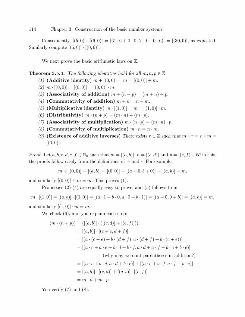
114 Chapter 3: Construction of the basic number systems
Consequently, [(5, 0)] · [(6, 0)] = [(5 · 6 + 0 · 0, 5 · 0 + 0 · 6)] = [(30, 0)], as expected.
Similarly compute [(5, 0)] · [(0, 6)].
We next prove the basic arithmetic laws on Z.
Theorem 3.5.4. The following identities hold for all m,n, p ∈ Z:
(1) (Additive identity) m+ [(0, 0)] = m = [(0, 0)] +m.
(2) m · [(0, 0)] = [(0, 0)] = [(0, 0)] ·m.
(3) (Associativity of addition) m+ (n+ p) = (m+ n) + p.
(4) (Commutativity of addition) m+ n = n+m.
(5) (Multiplicative identity) m · [(1, 0)] = m = [(1, 0)] ·m.
(6) (Distributivity) m · (n+ p) = (m · n) + (m · p).(7) (Associativity of multiplication) m · (n · p) = (m · n) · p.(8) (Commutativity of multiplication) m · n = n ·m.
(9) (Existence of additive inverses) There exists r ∈ Z such that m+r = r+m =
[(0, 0)].
Proof. Let a, b, c, d, e, f ∈ N0 such that m = [(a, b)], n = [(c, d)] and p = [(e, f)]. With this,
the proofs follow easily from the definitions of + and ·. For example,
m+ [(0, 0)] = [(a, b)] + [(0, 0)] = [(a+ 0, b+ 0)] = [(a, b)] = m,
and similarly [(0, 0)] +m = m. This proves (1).
Properties (2)-(4) are equally easy to prove, and (5) follows from
m · [(1, 0)] = [(a, b)] · [(1, 0)] = [(a · 1 + b · 0, a · 0 + b · 1)] = [(a+ 0, 0 + b)] = [(a, b)] = m,
and similarly [(1, 0)] ·m = m.
We check (6), and you explain each step:
(m · (n+ p)) = ([(a, b)] · ([(c, d)] + [(e, f)]))
= [(a, b)] · [(c+ e, d+ f)]
= [(a · (c+ e) + b · (d+ f), a · (d+ f) + b · (c+ e))]
= [(a · c+ a · e+ b · d+ b · f, a · d+ a · f + b · c+ b · e)](why may we omit parentheses in addition?)
= [(a · c+ b · d, a · d+ b · c)] + [(a · e+ b · f, a · f + b · e)]= [(a, b)] · [(c, d)] + [(a, b)] · [(e, f)]
= m · n+m · p.
You verify (7) and (8).

Section 3.5: Construction of Z, arithmetic, and order on Z 115
(9) Set r = [(b, a)]. Then m+r = [(a, b)]+ [(b, a)] = [(a+ b, b+a)] = [(a+ b, a+ b)] =
[(0, 0)], and similarly r +m = [(0, 0)].
Notation 3.5.5. The additive inverse of the equivalence class [(a, b)] of (a, b) is the equiv-
alence class [(b, a)] of (b, a). The additive inverse of an element m is always denoted −m.
Notation 3.5.6. Furthermore, for any a, b ∈ N0, by trichotomy on N0 (Theorem 3.3.3),
exactly one of the following three conditions is satisfied:
a < b, a = b, b < a.
In the first two cases, by Theorem 3.3.5, there exists r ∈ N0 such that a+ r = b, and then
[(a, b)] = [(a, a+ r)] = [(0, r)], and in the last case there exists r ∈ N0 such that b+ r = a,
and then [(a, b)] = [(b+ r, b)] = [(r, 0)]. This proves that every element of Z can be written
as the equivalence class of [(a, b)] where a or b is 0.
Recall the identification of elements of N0 with elements in Z: n ∈ N0 is identified
with [(n, 0)]. Then with the last two paragraphs,
[(a, b)] = [(a, 0)] + [(0, b)] = a+ (−b),
and it is standard shorthand to write this as a−b. Thus in the future we will write elements
[(a, b)] in Z as a− b.
Theorem 3.5.7. Let m,n ∈ Z. Then (−m) · n = m · (−n) = −(m · n).
Proof. Observe that
m · (−n) +m · n = m · ((−n) + n) (by distributivity: Theorem 3.5.4 (6))
= m · 0 (by notation for additive inverses)
= 0 (by Theorem 3.5.4 (2)).
Similarly, m · n + m · (−n) = 0. Thus m · (−n) is an additive inverse of m · n, and by
uniqueness of inverses (Theorem 2.5.10), m · (−n) is the additive inverse of m · n, i.e.,
m · (−n) = −(m · n).
With that,
(−m) · n = n · (−m) (by commutativity of multiplication)
= −(n ·m) (by the previous paragraph).

116 Chapter 3: Construction of the basic number systems
Theorem 3.5.8. Let m,n ∈ Z. Then m · n = 0 if and only if m = 0 or n = 0.
Proof. We already proved that if m = 0 or n = 0, then m · n = 0.
Now suppose that m · n = 0. Write m = [(a, b)] with a, b ∈ N0. By Notation 3.5.6
we may assume that either a = 0 or b = 0. Write n = [(c, d)] for c, d ∈ N0.
If a = 0, then [(0, 0)] = 0 = m · n = [(0, b)] · [(c, d)] = [(b · d, b · c)]. This means (by
definition of ∼) that b · d = b · c. If b = 0, then m = [(0, 0)] = 0, and if b 6= 0, then by
Theorem 3.4.2, d = c, so that n = [(c, d)] = [(0, 0)] = 0.
Similarly, if b = 0, then either m = 0 or n = 0. But a = 0 or b = 0 covers all the
possible cases for elements of Z, so we’ve proved the theorem.
Definition 3.5.9. (Order on Z) Define a relation ≤ on Z as follows: [(a, b)] ≤ [(c, d)] if
a + d ≤ b + c, where the latter ≤ is the already known relation on N0 (see Section 3.3).
Similarly define <,≥, >.
It is left to the reader to verify the following:
Lemma 3.5.10.
(1) ≤ on Z is well-defined (this means that if one picks different representatives of the
equivalence classes, ≤ for one pair holds if and only if it holds for the other pair).
(2) ≤,≥ are reflexive and transitive but not symmetric.
(3) <,> are transitive but not reflexive and not symmetric.
(4) If m ∈ Z and 0 ≤ m, then m ∈ N0.
(5) If m ∈ Z and m ≤ 0, then −m ∈ N0.
Theorem 3.5.11. The following properties hold on Z:
(1) (Trichotomy) For any m,n ∈ Z, exactly one of the following three conditions
holds:
(i) m = n.
(ii) m < n.
(iii) n < m.
(2) (Transitivity) For all m,n, p ∈ Z, m < n and n < p imply m < p.
(3) (Compatibility of < with addition) For all m,n, p ∈ Z, m < n implies m+p <
n+ p.
(4) (Compatibility of < with multiplication by positive numbers) For all
m,n, p ∈ Z, m < n and 0 < p imply mp < np.
Proof. Write m = [(a, b)], n = [(c, d)], and p = [(e, f)] for some a, b, c, d, e, f ∈ N0.
By Theorem 3.3.3, exactly one of the following three conditions holds:
a+ d < b+ c, a+ d = b+ c, b+ c < a+ d.
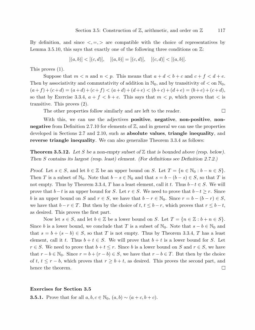
Section 3.5: Construction of Z, arithmetic, and order on Z 117
By definition, and since <,=, > are compatible with the choice of representatives by
Lemma 3.5.10, this says that exactly one of the following three conditions on Z:
[(a, b)] < [(c, d)], [(a, b)] = [(c, d)], [(c, d)] < [(a, b)].
This proves (1).
Suppose that m < n and n < p. This means that a + d < b + c and c + f < d + e.
Then by associativity and commutativity of addition in N0, and by transitivity of < on N0,
(a+f) + (c+d) = (a+d) + (c+f) < (a+d) + (d+ e) < (b+ c) + (d+ e) = (b+ e) + (c+d),
so that by Exercise 3.3.4, a + f < b + e. This says that m < p, which proves that < is
transitive. This proves (2).
The other properties follow similarly and are left to the reader.
With this, we can use the adjectives positive, negative, non-positive, non-
negative from Definition 2.7.10 for elements of Z, and in general we can use the properties
developed in Sections 2.7 and 2.10, such as absolute values, triangle inequality, and
reverse triangle inequality. We can also generalize Theorem 3.3.4 as follows:
Theorem 3.5.12. Let S be a non-empty subset of Z that is bounded above (resp. below).
Then S contains its largest (resp. least) element. (For definitions see Definition 2.7.2.)
Proof. Let s ∈ S, and let b ∈ Z be an upper bound on S. Let T = {n ∈ N0 : b − n ∈ S}.Then T is a subset of N0. Note that b− s ∈ N0 and that s = b− (b− s) ∈ S, so that T is
not empty. Thus by Theorem 3.3.4, T has a least element, call it t. Thus b− t ∈ S. We will
prove that b− t is an upper bound for S. Let r ∈ S. We need to prove that b− t ≥ r. Since
b is an upper bound on S and r ∈ S, we have that b− r ∈ N0. Since r = b− (b− r) ∈ S,
we have that b− r ∈ T . But then by the choice of t, t ≤ b− r, which proves that r ≤ b− t,as desired. This proves the first part.
Now let s ∈ S, and let b ∈ Z be a lower bound on S. Let T = {n ∈ Z : b + n ∈ S}.Since b is a lower bound, we conclude that T is a subset of N0. Note that s− b ∈ N0 and
that s = b + (s − b) ∈ S, so that T is not empty. Thus by Theorem 3.3.4, T has a least
element, call it t. Thus b + t ∈ S. We will prove that b + t is a lower bound for S. Let
r ∈ S. We need to prove that b+ t ≤ r. Since b is a lower bound on S and r ∈ S, we have
that r− b ∈ N0. Since r = b+ (r− b) ∈ S, we have that r− b ∈ T . But then by the choice
of t, t ≤ r − b, which proves that r ≥ b + t, as desired. This proves the second part, and
hence the theorem.
Exercises for Section 3.5
3.5.1. Prove that for all a, b, c ∈ N0, (a, b) ∼ (a+ c, b+ c).

118 Chapter 3: Construction of the basic number systems
3.5.2. Suppose that a, b, c, d ∈ N0 such that (a, b) ∼ (c, d) and a ≥ c. Prove that there
exists e ∈ N0 such that a = c+ e and b = d+ e.
3.5.3. Convince yourself that Z as defined in Definition 3.5.2 is the same as the familiar
set of all integers.
3.5.4. (Cancellation in Z) Let m,n, p ∈ Z.
i) If m+ p = n+ p, prove that m = n. (Hint: Theorem 2.5.16.)
ii) If p 6= 0 and m · p = n · p, prove that m = n. (Note that Theorem 2.5.16 is
inapplicable.)
3.5.5. Prove that if (a, b) ∼ (c, d) then (a, c) ∼ (b, d).
3.5.6. Let a, b, c, d ∈ N0. Suppose that [(b, a)] < [(c, d)]. Prove that [(a, b)] > [(d, c)] and
[(a, b)] + [(c, d)] > [(0, 0)].
3.5.7. Prove (2), (3), (4), (7), (8) in Theorem 3.5.4.
3.5.8. Prove Lemma 3.5.10.
3.5.9. Prove (3) and (4) in Theorem 3.5.11.
3.6 Construction of the ordered field Q of rational numbers
We next define the set Q, arithmetic, and order on it, and we show that Q is a field.
Elements of course correspond to the familiar rational numbers.
The following is a rehashing of the construction of Q from Z first given in Exer-
cise 2.3.10. The relation o on Z× (Z \ {0}), given by
(m,n) o (m′, n′) if m · n′ = m′ · n,
is an equivalence relation. The reader may wish to go through the details of the proof, to
check that only those properties of Z are used that we have proved in the previous section,
and that no “well-known” knowledge creeps into the proof.
Remark 3.6.1. For any a ∈ Z and b, c ∈ Z \ {0}, the equivalence class [(ca, cb)] equals
the equivalence class [(a, b)]. In particular, by possibly taking a negative c, we may always
choose a representative of any equivalence class in Z× N+.

Section 3.6: Construction of the ordered field Q of rational numbers 119
Definition 3.6.2. We define the set of all equivalence classes of this relation to be Q. The
elements of Q are called rational numbers.
We have a natural inclusion of Z into Q (and thus of N0 into Q) by identifying m ∈ Zwith [(m, 1)]. Note that if m,n ∈ Z are distinct, so are [(m, 1)] and [(n, 1)], so that Z is
indeed identified with a natural subset of Q. But Q is strictly larger: [(1, 2)] is not equal
to [(m, 1)] for any m ∈ Z. More about the familiar rational numbers is in Notation 3.6.5.
We declare the following binary operations + and · on elements of Z× (Z \ {0}):
(m,n) + (p, q) = (m · q + p · n, n · q), (m,n) · (p, q) = (m · p, n · q).
(The + and · inside the pair entries are the operations on Z; the other + and · are what
we are defining here.) We show next that the new + and · are compatible with o:
Theorem 3.6.3. Let m,m′, n, n′, p, p′, q, q′ ∈ N0 such that (m,n) o (m′, n′) and (p, q) o(p′, q′). Then
((m,n) + (p, q)) o ((m′, n′) + (p′, q′)) ,
and ((m,n) · (p, q)) o ((m′, n′) · (p′, q′)) .
Proof. By assumption, m · n′ = m′ · n and p · q′ = p′ · q. Then (you explain each step):
(m · q + p · n) · (n′ · q′) = (n′ · q′) · (m · q + p · n)
= (n′ · q′) · (m · q) + (n′ · q′) · (p · n)
= (q′ · n′) · (m · q) + n′ · (q′ · (p · n))
= q′ · (n′ · (m · q)) + n′ · ((q′ · p) · n)
= q′ · ((n′ ·m) · q) + n′ · ((p · q′) · n)
= q′ · ((m · n′) · q) + n′ · ((p′ · q) · n)
= q′ · ((m′ · n) · q) + n′ · (p′ · (q · n))
= q′ · (m′ · (n · q)) + n′ · (p′ · (n · q))= (q′ ·m′) · (n · q) + (n′ · p′) · (n · q)= (n · q) · (q′ ·m′) + (n · q) · (n′ · p′)= (n · q) · (m′ · q′) + (n · q) · (p′ · n′)= (n · q) · (m′ · q′ + p′ · n′)= (m′ · q′ + p′ · n′) · (n · q).
This says that
(m · q + p · n, n · q),= (m′ · q′ + p′ · n′, n′ · q′),
which in turn says that ((m,n) + (p, q)) o ((m′, n′) + (p′, q′)).
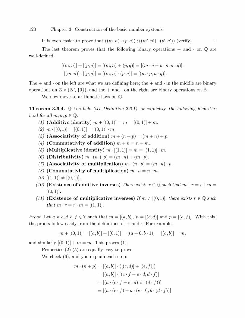
120 Chapter 3: Construction of the basic number systems
It is even easier to prove that ((m,n) · (p, q)) o ((m′, n′) · (p′, q′)) (verify).
The last theorem proves that the following binary operations + and · on Q are
well-defined:
[(m,n)] + [(p, q)] = [(m,n) + (p, q)] = [(m · q + p · n, n · q)],[(m,n)] · [(p, q)] = [(m,n) · (p, q)] = [(m · p, n · q)].
The + and · on the left are what we are defining here; the + and · in the middle are binary
operations on Z× (Z \ {0}), and the + and · on the right are binary operations on Z.
We now move to arithmetic laws on Q.
Theorem 3.6.4. Q is a field (see Definition 2.6.1), or explicitly, the following identities
hold for all m,n, p ∈ Q:
(1) (Additive identity) m+ [(0, 1)] = m = [(0, 1)] +m.
(2) m · [(0, 1)] = [(0, 1)] = [(0, 1)] ·m.
(3) (Associativity of addition) m+ (n+ p) = (m+ n) + p.
(4) (Commutativity of addition) m+ n = n+m.
(5) (Multiplicative identity) m · [(1, 1)] = m = [(1, 1)] ·m.
(6) (Distributivity) m · (n+ p) = (m · n) + (m · p).(7) (Associativity of multiplication) m · (n · p) = (m · n) · p.(8) (Commutativity of multiplication) m · n = n ·m.
(9) [(1, 1)] 6= [(0, 1)].
(10) (Existence of additive inverses) There exists r ∈ Q such that m+r = r+m =
[(0, 1)].
(11) (Existence of multiplicative inverses) If m 6= [(0, 1)], there exists r ∈ Q such
that m · r = r ·m = [(1, 1)].
Proof. Let a, b, c, d, e, f ∈ Z such that m = [(a, b)], n = [(c, d)] and p = [(e, f)]. With this,
the proofs follow easily from the definitions of + and ·. For example,
m+ [(0, 1)] = [(a, b)] + [(0, 1)] = [(a+ 0, b · 1)] = [(a, b)] = m,
and similarly [(0, 1)] +m = m. This proves (1).
Properties (2)-(5) are equally easy to prove.
We check (6), and you explain each step:
m · (n+ p) = [(a, b)] · ([(c, d)] + [(e, f)])
= [(a, b)] · [(c · f + e · d, d · f)]
= [(a · (c · f + e · d), b · (d · f))]
= [(a · (c · f) + a · (e · d), b · (d · f))]

Section 3.6: Construction of the ordered field Q of rational numbers 121
= [(a, b)] · [(c, d)] + [(a, b)] · [(e, f)]
= m · n+m · p.
You verify (7) and (8).
(9) By the properties of Z, 0 · 1 = 0 6= 0+ = 1 = 1 · 1, so that (0, 1) 6 o (1, 1), so that
[(0, 1)] 6= [(1, 1)] in Q.
(10) By definition of m and Q, [(−a, b)] ∈ Q, and m+[(−a, b)] = [(a·b+(−a)·b, b·b)] =
[(b · a + b · (−a), b · b)] = [(b · (a + (−a)), b · b)] = [(b · 0, b · b)] = [(0, b · b)] = [(0, 1)], and
similarly [(−a, b)] +m = [(0, 1)]. Thus additive inverses exist in Q.
(11) By assumption [(a, b)] 6= [(0, 1)], This means that a · 1 6= 0 · b, so that a 6= 0.
Then [(b, a)] ∈ Q, and [(a, b)] · [(b, a)] = [(a · b, b · a)] = [(a · b, a · b)] = [(1, 1)]. Similarly
[(b, a)] · [(a, b)] = [(1, 1)].
Notation 3.6.5. The additive inverse of the equivalence class [(a, b)] of (a, b) is [(−a, b)],and the multiplicative inverse of non-zero [(a, b)] is [(b, a)]. For an element m, its additive
inverse is always denoted −m, and the multiplicative inverse, when it exists, is written
m−1. Thus for any n ∈ Z, by identifying n with [(n, 1)] in Q, the additive inverse is −n =
−[(n, 1)] = [(−n, 1)], and if n 6= 0, the multiplicative inverse is n−1 = [(n, 1)]−1 = [(1, n)].
Thus, under our identifications, any element [(m,n)] in Q is equal to
[(m,n)] = [(m, 1)] · [(1, n)] = m · n−1,
and it is standard shorthand to write this as m/n. Thus in the future we will write elements
[(m,n)] in Q as m/n, and whenever m,n ∈ Z and n 6= 0, then [(m,n)] = m/n ∈ Q. By
Remark 3.6.1 we may even assume that n > 0.
Theorem 3.6.6. (Cancellation laws in Q) Let m,n, p ∈ Q.
(1) If m+ p = n+ p, then m = n.
(2) If m · p = n · p and if p 6= 0, then m = n.
Proof. Since every p ∈ Q has an additive inverse and since every non-zero p ∈ Q has a
multiplicative inverse, both parts are simply special cases of Theorem 2.5.16.
Theorem 3.6.7. Q is an ordered field (see Definition 2.7.10) with the order < given by:
[(a, b)] < [(c, d)] if
{ad < bc; if bd > 0;ad > bc; if bd < 0.
Proof. Theorem 3.6.4 proves that Q is a field. Now we prove that Q is ordered.
First we need to prove that < is well-defined. Let m,n ∈ Q. Write m = [(a, b)] =
[(a′, b′)], n = [(c, d)] = [(c′, d′)]. By definition of Q, a′b = ab′ and c′d = cd′. By associativity
and commutativity of multiplication in Z, (bd)(b′d′)(b′c′ − a′d′) = bb′dd′(b′c′ − a′d′) =
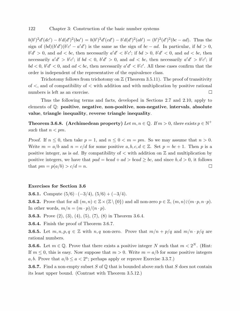
122 Chapter 3: Construction of the basic number systems
b(b′)2d′(dc′) − b′d(d′)2(ba′) = b(b′)2d′(cd′) − b′d(d′)2(ab′) = (b′)2(d′)2(bc − ad). Thus the
sign of (bd)(b′d′)(b′c′ − a′d′) is the same as the sign of bc − ad. In particular, if bd > 0,
b′d′ > 0, and ad < bc, then necessarily a′d′ < b′c′; if bd > 0, b′d′ < 0, and ad < bc, then
necessarily a′d′ > b′c′; if bd < 0, b′d′ > 0, and ad < bc, then necessarily a′d′ > b′c′; if
bd < 0, b′d′ < 0, and ad < bc, then necessarily a′d′ < b′c′. All these cases confirm that the
order is independent of the representative of the equivalence class.
Trichotomy follows from trichotomy on Z (Theorem 3.5.11). The proof of transitivity
of <, and of compatibility of < with addition and with multiplication by positive rational
numbers is left as an exercise.
Thus the following terms and facts, developed in Sections 2.7 and 2.10, apply to
elements of Q: positive, negative, non-positive, non-negative, intervals, absolute
value, triangle inequality, reverse triangle inequality.
Theorem 3.6.8. (Archimedean property) Let m,n ∈ Q. If m > 0, there exists p ∈ N+
such that n < pm.
Proof. If n ≤ 0, then take p = 1, and n ≤ 0 < m = pm. So we may assume that n > 0.
Write m = a/b and n = c/d for some positive a, b, c, d ∈ Z. Set p = bc + 1. Then p is a
positive integer, as is ad. By compatibility of < with addition on Z and multiplication by
positive integers, we have that pad = bcad+ ad > bcad ≥ bc, and since b, d > 0, it follows
that pm = p(a/b) > c/d = n.
Exercises for Section 3.6
3.6.1. Compute (5/6) · (−3/4), (5/6) + (−3/4).
3.6.2. Prove that for all (m,n) ∈ Z× (Z\{0}) and all non-zero p ∈ Z, (m,n) o (m ·p, n ·p).In other words, m/n = (m · p)/(n · p).3.6.3. Prove (2), (3), (4), (5), (7), (8) in Theorem 3.6.4.
3.6.4. Finish the proof of Theorem 3.6.7.
3.6.5. Let m,n, p, q ∈ Z with n, q non-zero. Prove that m/n + p/q and m/n · p/q are
rational numbers.
3.6.6. Let m ∈ Q. Prove that there exists a positive integer N such that m < 2N . (Hint:
If m ≤ 0, this is easy. Now suppose that m > 0. Write m = a/b for some positive integers
a, b. Prove that a/b ≤ a < 2a; perhaps apply or reprove Exercise 3.3.7.)
3.6.7. Find a non-empty subset S of Q that is bounded above such that S does not contain
its least upper bound. (Contrast with Theorem 3.5.12.)
Section 3.7: Construction of the field R of real numbers 123
3.7 Construction of the field R of real numbers
In this section we construct real numbers from Q via Dedekind cuts: a Dedekind cut
stands for a real number and vice versa. We establish the familiar arithmetic on R, and
in the subsequent section we show that R is an ordered field with further good properties.
To go through these two sections carefully would take many hours. I typically spend 1.5
class hours going through them, asking the students not to take notes but instead to nod
vigorously in agreement and awe at all the constructions and claims. I expect the students
to get the gist of the construction, a conviction that any arithmetic and order property
of real numbers can be verified if necessary, but I do not expect the students to have
gone through all the details. Furthermore, I do not use the standard Dedekind cuts, as
arithmetic with them is messier (see Exercise 3.7.16).
Definition 3.7.1. A Dedekind cut is a pair (L,R) with the following properties:
(1) L,R are non-empty subsets of Q.
(2) For all l ∈ L and all r ∈ R, l < r.
(3) For all l ∈ L, there exists l′ ∈ L such that l < l′.
(4) For all r ∈ R, there exists r′ ∈ R such that r′ < r.
(5) L ∪R is either Q or Q \ {m} for some m ∈ Q. In case L ∪R = Q \ {m}, then for
all l ∈ L and all r ∈ R, l < m < r.
By condition (2) and the trichotomy property of < on Q, L ∩R = ∅.We can visualize a Dedekind cut (L,R) as the separation of the rational number
line into the left and right parts, and the separation comes either at a rational number m,
or possibly at something else. The letters “L” and “R” are mnemonics for “left” and
“right”.
An easy consequence of the definition is that if l ∈ L and x ∈ Q with x < l, then
x ∈ L, and similarly that if r ∈ R and x ∈ Q with x > l, then x ∈ R. (See Exercise 3.7.1.)
Examples and non-examples 3.7.2.
(1) (Q \ {0}, {0}) is not a Dedekind cut: it violates conditions (2) and (4).
(2) ({x ∈ Q : x2 < 2}, {x ∈ Q : x2 > 2}) is not a Dedekind cut: it violates condi-
tion (2).
(3) ({x ∈ Q : x < 0}, {x ∈ Q : x > 0}) is a Dedekind cut.
(4) ({x ∈ Q : x ≤ 0}, {x ∈ Q : x > 0}) is not a Dedekind cut: it violates condition (3).
124 Chapter 3: Construction of the basic number systems
Theorem 3.7.3. Let (L,R) be a Dedekind cut. Let x ∈ Q.
(1) Suppose that x < l for some l ∈ L. Then x ∈ L.
(2) Suppose that x > r for some r ∈ R. Then x ∈ R.
Proof. We only prove the first part. By condition (2), x is not in R, and by condition (5),
x ∈ L.
Definition 3.7.4. We define R to be the set of all Dedekind cuts. Elements of R are
therefore Dedekind cuts, but more normally, the elements are called real numbers.
The first goal is to prove that Q is a subset of R, at least under an identification of
elements of Q with Dedekind cuts.
Theorem 3.7.5. For any m ∈ Q, Dm = ({l ∈ Q : l < m}, {r ∈ Q : r > m}) is a Dedekind
cut.
Proof. Let L = {l ∈ Q : l < m}, R = {r ∈ Q : r > m}. By Theorem 2.7.11, 1 > 0, so
that by compatibility of < and + on Q, m+ 1 > m and m− 1 < m. Thus m− 1 ∈ L and
m+ 1 ∈ R. Thus L and R are not empty.
By trichotomy on Q, for every r ∈ Q, exactly one of the following holds: r < m,
r = m, r > m. So L∪R = Q\{m}. By definition, for any l ∈ L and any r ∈ R, l < m < r,
and by transitivity, we conclude that l < r.
If l ∈ L, then l < m, and by Exercise 2.7.15, l′ = (l + m)/2 is a rational number
strictly larger than l and strictly smaller than m. Thus, l < l′ ∈ L, and condition (3) of
Dedekind cuts holds. Similarly, for any r ∈ R, (r+m)/2 is in R and strictly smaller than r,
so that condition (4) of Dedekind cuts is satisfied.
Remark 3.7.6. If m,n are distinct in Q, say m < n, then by Exercise 2.7.15, (m+n)/2 is
in the right side of Dm and the left side of Dn, so that Dm and Dn are also distinct. This
gives a natural inclusion of Q into R (and thus of N0, N+, and Z into R) by identifying
m ∈ Q with the Dedekind cut Dm. Thus we can think of Q as a subset of R.
Many differences between Q and R are in Section 3.8. Here we point out that R is
strictly bigger than Q. Namely, ({x ∈ Q : x2 < 2 or x < 0}, {x ∈ Q : x2 ≥ 2 and x ≥ 0})is a Dedekind cut that is not of the form Dm for any m ∈ Q (Exercise 3.7.5).

Section 3.7: Construction of the field R of real numbers 125
Theorem 3.7.7. Let L be a non-empty proper subset of Q such that for all l ∈ L and all
x ∈ Q, if x < l then x ∈ L. Then there exists a unique subset R of Q such that (L,R) is a
Dedekind cut.
Let R be a non-empty proper subset of Q such that for all r ∈ R and all x ∈ Q, if
x > r then x ∈ R. Then there exists a unique subset L of Q such that (L,R) is a Dedekind
cut.
Proof. We only prove the first part. Set R′ = Q \ L.
If condition (4) of Dedekind cuts holds for (L,R′), let R = R′. Otherwise, there
exists m ∈ R′ such that for all r′ ∈ R′, r′ ≥ m. In this case set R = R′ \ {m}. Now let
r ∈ R. Then r > m. By Exercise 2.7.15, (r + m)/2 is a rational number strictly larger
than m and strictly smaller than r, so that by assumption (r+m)/2 ∈ R. Thus condition
(4) of Dedekind cuts holds for (L,R).
Since L is a proper non-empty subset of Q, so is R′, and even the modified R in
the previous paragraph. If l ∈ L and r ∈ R, by construction l 6= r and even l < r. Thus
conditions (1) and (2) hold, and condition (3) holds by assumption. Furthermore, condition
(5) holds by construction as well.
Now we turn to arithmetic on R.
Definition 3.7.8. Let A and B be subsets of Q. Define
A+B = {a+ b : a ∈ A and b ∈ B},−A = {−a : a ∈ A},A−B = {a− b : a ∈ A and b ∈ B} = A+ (−B),
A ·B = {a · b : a ∈ A and b ∈ B}.
Lemma 3.7.9. Let (L1, R1) and (L2, R2) be Dedekind cuts. Then (L1 + L2, R1 + R2) is
a Dedekind cut.
Proof. Since L1, L2, R1, R2 are non-empty subsets of Q, then L1 + L2, R1 + R2 are non-
empty subsets of Q as well. Let l ∈ L1 + L2 and r ∈ R1 + R2. Then l = l1 + l2 and
r = r1 + r2 for some li ∈ Li and ri ∈ Ri (i = 1, 2). Then l1 < r1 and l2 < r2, so that
l = l1 + l2 < l1 + r2 < r1 + r2 = r, and by transitivity of < on Q, l < r. Thus conditions
(1) and (2) of Dedekind cuts hold.
Conditions (3) and (4) hold similarly. Furthermore, if l ∈ L1 + L2 and x ∈ Qwith x < l, then we claim that x ∈ L1 + L2. Namely, write l = l1 + l2 for some li ∈ Li,i = 1, 2. By assumption we have that x−l+l1 < l1, and since (L1, R1) is a Dedekind cut, by
Exercise 3.7.1, we conclude that x−l+l1 ∈ L1. Thus x = x−l+l = x−l+l1 +l2 ∈ L1 +L2.
Similarly, whenever r ∈ R1 +R2 and x ∈ Q with r < x, then x ∈ R1 +R2.
126 Chapter 3: Construction of the basic number systems
It remains to prove Condition (5) of Dedekind cuts for (L1 +L2, R1 +R2). Let x ∈ Qand suppose that x 6∈ (L1 +L2)∪ (R1 +R2). We will prove that (L1 +L2, R1 +R2) is the
Dedekind cut Dx. For this we need to prove that any y ∈ Q not in (L1 + L2) ∪ (R1 +R2)
equals x. By Remark 3.6.1 and Notation 3.6.5 we may write x = mn , y = p
n for some
m,n, p ∈ Z, with n > 0. By the definition of Dedekind cuts the sets Si = {r ∈ Z : rn ∈ Ri}are bounded below, so that Si has a least element ai ∈ Z by Theorem 3.5.12. Thus c
n ∈ Rifor all integers c ≥ ai, and c
n 6∈ Ri for all integers c < ai. In particular, cn ∈ R1 + R2 for
all integers c ≥ a1 + a2. If (ai − 1)/n ∈ Li for i = 1, 2, then cn ∈ L1 + L2 for all integers
c ≤ a1 +a2−2, so that necessarily x = y = a1+a2−1n . So say that (a1−1)/n 6∈ L1. Then by
the definition of Dedekind cuts we have that L1 = D(a1−1)/n. If also (a2− 1)/n 6∈ L2, then
L2 = D(a2−1)/n, cn ∈ L1 + L2 for all integers c ≤ a1 + a2 − 4, a1+a2−3
n = 2a1−32n + 2a2−3
2n ∈L1 + L2, a1+a2−1
n = 2a1−12n + 2a2−1
2n ∈ R1 + R2, so that x = y = a1+a2−2n . The remaining
case is where L1 = D(a1−1)/n and L2 6= D(a2−1)/n. If L2 = Dr for some rational number
r, then by possibly taking a multiple of n we may assume that r is of the form qn for
some integer q, but then we are in the previous case. So we may suppose that (L2, R2)
is not a rational number. Then 2a2−1n is either in R2 or in L2. If it is in R2, then
a1+a2−1n = 2a1−1
2n + 2a2−12n ∈ R1 + R2, so that necessarily x = y = a1+a2−2
n , and if it is in
L2, then a1+a2−2n = 2a1−3
2n + 2a2−12n ∈ L1 + L2, so that x = y = a1+a2−1
n . Thus Condition
(5) holds.
Thus we can define addition on R by
(L1, R1) + (L2, R2) = (L1 + L2, R1 +R2).
There are two different meanings to “+” above: on the right side, + acts on two sets of
rational numbers, and on the left, + stands for the new sum.
The proof of the following is left as an exercise.
Theorem 3.7.10. Addition on R, as defined above, is commutative and associative. The
additive identity is D0 = (Q−,Q+), and the additive inverse of any (L,R) ∈ R is (−R,−L)
(recall Definition 3.7.8).
Naturally we will write the additive identity D0 of R as 0, and for any x ∈ R, we
write its additive inverse as −x.
Additions on Q and R are compatible, in the following sense:
Theorem 3.7.11. For any m,n ∈ Q, Dm + Dn = Dm+n (the first + is in R, the second
in Q).
Proof. We know that Dm +Dn is a Dedekind cut, and we can write it as (L,R).
We first prove that R = {r ∈ Q : r > m + n}. Let r ∈ R. By definition of addition
on R, r = rm + rn for some rm > m and rn > n. But then by compatibility of addition in

Section 3.7: Construction of the field R of real numbers 127
Q with >,
r = rm + rn > rm + n > m+ n,
and by transitivity, r > m+ n. This proves that R ⊆ {r ∈ Q : r > m+ n}. Now suppose
that r ∈ Q with r > m+n. Set rm = r−m−n2 +m and rn = r−m−n
2 +n. By compatibility of
< with addition on Q, we know that r−m−n > 0. By Theorem 2.7.11 we know that 1 > 0,
so that again by compatibility, 2 = 1 + 1 > 0. Then by Theorem 2.10.4, r−m−n2 > 0, so
that rm > m and rn > n. Finally, rm+rn = r, which proves that {r ∈ Q : r > m+n} ⊆ R.
Thus R = {r ∈ Q : r > m+ n}.Then by uniqueness of Dedekind cuts, Dm +Dn = Dm+n.
Multiplication on R is more complicated, but if one keeps in mind the “expected”
facts about real numbers, the following definition of multiplication on Dedekind cuts is
natural (see Exercise 3.7.12 for an alternate formulation):
(L,R) · (L′, R′) =
( , R ·R′), if R and R′ contain only positive elements of Q;(R · L′, ), if R and −L′ contain only positive elements;(L ·R′, ), if R′ and −L contain only positive elements;( , L · L′), if neither R nor R′ contains only positive elements,
where in each case is the unique subset of Q that makes the result a Dedekind cut. It is
only possible to find such a if the non-blank part on the right side satisfies the conditions
in Theorem 3.7.7. It is left to Exercise 3.7.10 to prove that.
Clearly · is a commutative operation, and it is easy to show that D1 = ({x ∈ Q : x <
1}, {x ∈ Q : x > 1}) is a multiplicative identity (and therefore the unique multiplicative
identity by Theorem 2.5.5). The following are multiplicative inverses for (L,R) 6= D0:
(L,R)−1 =
{( , {1/r : r ∈ R}), if R contains only positive elements of Q;({1/l : l ∈ L}, ), if R does not contain only positive elements.
If all elements of R are positive, we are certainly not dividing by 0 in the first case. In the
second case, by Exercise 3.7.1, L contains only negative elements, and so again we are not
dividing by 0. It is now straightforward to verify that the listed Dedekind cut is indeed
the multiplicative inverse.
I will let the reader verify that for all m,n ∈ Q, Dm ·Dn = Dmn.
Proofs of associativity of multiplication and of distributivity of multiplication over
addition are more involved. With the definition above, we would have to verify eight cases
for associativity, and many cases for distributivity, depending on whether the left parts
of the various Dedekind cuts contain positive elements. Yes, this can be done, but it is
tedious work. We provide a different proof in these notes that is not a brute-force attack
but is more conceptual and gives side results as a bonus. We first need a lemma.

128 Chapter 3: Construction of the basic number systems
Lemma 3.7.12. For any Dedekind cuts x, y, (−x) · y = −(x · y) = x · (−y).
Proof. Write x = (L,R) and y = (L′, R′).
If L,L′ contain positive elements, then −R,−R′ do not contain positive elements,
and by definition of multiplication,
(x · y) + ((−x) · y) = ((L,R) · (L′, R′)) + ((−R,−L) · (L′, R′))= ( , R ·R′) + ((−R) ·R′, )
= ( , R ·R′) + (−(R ·R′), ).
By Theorem 3.7.7, the left side U of ( , R ·R′) is either Q \ (R ·R′) or Q \ ((R ·R′)∪ {m})for some rational number m. Since R · R′ consists of positive numbers strictly greater
than numbers in Q \ (R · R′) it follows that the left side is contained in the set Q− of all
negative rational numbers. Furthermore, let r be any negative rational number. We want
to find x ∈ U and y ∈ R · R′ such that x − y = r. Let x ∈ U and y ∈ R · R′. Write
r = r0/n, x = x0/n and y = y0/n for some integers r0, x0, y0, n, with n positive. By
possibly changing x and y but not n, we may assume that x0 is the largest possible and y0
the smallest possible. If (y0−1)/n ∈ U , then y0 = x0+1, and y−x = y0/n−x0/n = 1/n. If
instead (y0−1)/n 6∈ U , then (y0−1)/n = m, so that (2y0−1)/2n ∈ R·R′, (2y0−3)/2n ∈ U ,
and (2y0− 3)/2n− (2y0− 1)/2n = 1/2n. Thus we have found a representation of r as r0/n
for some positive integer n and some negative integer r0 such that for some integers x0, y0,
x0/n ∈ U , y0/n ∈ R ·R′, and x0/n− y0/n = 1/n. But then (y0 + (r − 1))/n ∈ R ·R′ and
x0/n− (y0 + (r0 − 1))/n = r0/n = r. This proves that the left side of the Dedekind cut in
the display equals Q−. Thus (x · y) + ((−x) · y) = D0. By commutativity of addition this
also gives ((−x) · y) + (x · y) = D0, ((−x) · y) = −(x · y).
If L contains positive elements but L′ does not, then
(x · y) + ((−x) · y) = ((L,R) · (L′, R′)) + ((−R,−L) · (L′, R′))= (R · L′, ) + ( ,−(R · L′)),
and similarly to the previous case, this is D0, so again ((−x) · y) = −(x · y).
The remaining cases of ((−x) · y) = −(x · y) are proved similarly. Then by com-
mutativity of multiplication, x · (−y) = (−y) · x, and by the established case this equals
−(y · x) = −(x · y).
Theorem 3.7.13. R is a field containing Q.
Proof. We have already verified that for elements of Q, arithmetic on R agrees with
arithmetic on Q.
The only parts left to prove are that multiplication is associative and that it dis-
tributes over addition. Let x = (L,R), y = (L′, R′), z = (L′′, R′′) be in R.

Section 3.7: Construction of the field R of real numbers 129
To prove that x · (y · z) = (x · y) · z, it suffices to prove that the additive inverses of
the two products are identical. By Lemma 3.7.12, we may then in each product replace
x = (L,R) by −x = (−R,−L), and similarly for y by −y and z by −z. Note that R does
not contain only positive numbers if and only if −L contains only positive numbers, so via
these replacements we may assume that R,R′, R′′ all contain only positive elements. But
then x · (y · z) = ( , L · (L′ ·L′′)), which is by associativity of multiplication on Q the same
as ( , (L · L′) · L′′) = (x · y) · z. This proves associativity of multiplication.
To prove that x ·(y+z) = (x ·y)+(x ·z), we may similarly assume that R and R′+R′′
contain only positive numbers. Then either R′ or R′′ contains only positive elements, and
by commutativity of addition we may assume that R′ contains only positive elements. From
assumptions we have x · (y + z) = ( , R · (R′ + R′′)). If a ∈ R, b ∈ R′ and c ∈ R′′, then
a ·(b+c) = a ·b+a ·c by distributivity in Q, which proves that R ·(R′+R′′) ⊆ R ·R′+R ·R′′.Suppose that in addition R′′ contains only positive numbers. Let r1, r2 ∈ R, r′ ∈ R′,
r′′ ∈ R′′. Then (r1 ·r′+r2 ·r′′)/(r′+r′′) is a rational number. If (r1 ·r′+r2 ·r′′)/(r′+r′′) < r1,
then by compatibility of multiplication with < on Q, r1 · r′ + r2 · r′′ < r1 · r′ + r1 · r′′,whence 0 < (r1 − r2) · r′′, which forces r1 > r2. By the same reasoning then necessarily
(r1 · r′+ r2 · r′′)/(r′+ r′′) ≥ r2, whence in any case (r1 · r′+ r2 · r′′)/(r′+ r′′) ≥ min{r1, r2}.It follows by Exercise 3.7.1 that (r1 ·r′+r2 ·r′′)/(r′+r′′) ∈ R, so that the arbitrary element
r1 ·r′+r2 ·r′′ of R·R′+R·R′′ is in R·(R′+R′′). This proves that R·(R′+R′′) = R·R′+R·R′′.Thus in this case x · (y + z) = ( , R ·R′ +R ·R′′) = ( , R ·R′) + ( , R ·R′′) x · y + x · z.
Now suppose that R′′ does not contain only positive numbers. Then −L′′ contains
only positive numbers. Thus by the previous case x · (y+z)+x · (−z) = x · ((y+z)+(−z)).By the already established associativity of addition, this is x ·y. But by Lemma 3.7.12 this
says that x · (y + z) = x · y + x · z.Certainly Q is a subset of R, and the addition and multiplication on R restrict to
the familiar addition and multiplication on Q.
The Dedekind cuts as in Theorem 3.7.5 are the familiar rational numbers, and if we
establish some good order on R, we should be able to order the other Dedekind cuts among
the rational ones as expected, to get that R consists of the familiar real numbers.
Exercises for Section 3.7
3.7.1. Let (L,R) be a Dedekind cut, l ∈ L, r ∈ R, and x ∈ Q. Prove the following:
i) If x ≤ l, then x ∈ L.
ii) If x ≥ r, then x ∈ R.
3.7.2. Prove that there exists no R ⊂ Q such that (Q− ∪ {0}, R) is a Dedekind cut.
Similarly, there exists no L ⊂ Q such that (L,Q+ ∪ {0}) is a Dedekind cut.
130 Chapter 3: Construction of the basic number systems
3.7.3. Let (L,R) be a Dedekind cut.
i) If m ∈ Q is the supremum of L, prove that R = Q \ (L ∪ {m}). If L does not have
a supremum in Q, prove that R = Q \ L.
ii) If m ∈ Q is the infimum of R, prove that L = Q \ (R ∪ {m}). If R does not have
an infimum in Q, prove that L = Q \R.
3.7.4. Let (L,R) be a Dedekind cut and let (L′, R′) = (L,R)·(L,R). Prove that R′ ⊆ Q≥0.
3.7.5. Prove that ({x ∈ Q : x2 < 2 or x < 0}, {x ∈ Q : x2 ≥ 2 and x ≥ 0}) is a Dedekind
cut. Prove that it is not of the form Dm = ({x ∈ Q : x < m}, {x ∈ Q : x > m}) for
any rational number m. (Hint: 2 is not the square of a rational number, as was proved
on page 21.)
3.7.6. If m and n are rational numbers, prove that Dm +Dn = Dm+n.
3.7.7. Let a = ({x ∈ Q : x < 0 and x2 > 2}, {x ∈ Q : x2 ≤ 2 or x > 0}), b = ({x ∈ Q :
x < 0 or x2 < 3}, {x ∈ Q : x2 ≥ 3 and x > 0}). Compute a+ b, a · b.
3.7.8. Prove Theorem 3.7.10.
3.7.9. Prove that if (L1, R1), . . . , (Ln, Rn) are finitely many Dedekind cuts, then
(∪nk=1Lk,∩nk=1Rk) is a Dedekind cut. Furthermore, this Dedekind cut equals (Lk, Rk) for
some k ∈ {1, . . . , n}.
3.7.10. Prove that multiplication on Dedekind cuts is well-defined.
3.7.11. Let (L,R) be a Dedekind cut. Prove that there exists z ∈ Q such that z ∈ R and
−z ∈ L. Prove in addition that for any a ∈ Q, there exists such z with z ≥ |a|.
3.7.12. For any set S ⊆ Q, define S+ = S ∩ Q+ and S− = S ∩ Q−. Prove that for any
Dedekind sets (L,R), (L′, R′),
(L,R)·(L′, R′) = (L− ·R′++R+ ·L′−+L+ ·L′++R− ·R′−, L− ·L′−+R− ·L′++L+ ·R′−+R+ ·R′+),
where it is understood that A+ ∅ = A and A · ∅ = ∅.
3.7.13. Prove that every positive real number is the square of some real number. (Use
Dedekind cuts.)
3.7.14. Let x, y ∈ R.
i) Prove that x2 = (−x)2.
ii) Suppose that x2 = y2. Prove that either x = y or x = −y.
*3.7.15. Let x, y ∈ R such that x3 = y3. Prove that x = y.

Section 3.8: Order on R, the least upper/greatest lower bound theorem 131
3.7.16. The standard Dedekind cut in the literature is defined as the pair (L,R) with
the following properties:
(1) L,R are non-empty subsets of Q.
(2) For all l ∈ L and all r ∈ R, l < r.
(3) For all l ∈ L, there exists l′ ∈ L such that l < l′.
(4) L ∪R = Q.
What should be the definition of the sum of two standard Dedekind cuts? With the
definition above, why does (L1, R1) + (L2, R2) = (L1 + L2, R1 +R2) not work? Why does
−(L,R) = (−R,−L) not work?
3.8 Order on R, the least upper/greatest lower bound theorem
Definition 3.8.1. We impose the following order on R: (L,R) ≤ (L′, R′) if L ⊆ L′, and
(L,R) < (L′, R′) if L( L′.
Theorem 3.8.2. R is an ordered field.
Proof. By Theorem 3.7.13, R is a field. Let (L,R), (L′, R′), (L′′, R′′) ∈ R.
If L 6⊆ L′, let l ∈ L \ L′. Let l′ ∈ L′. By Exercise 3.7.1 applied to the Dedekind cut
(L,R), l > l′ and l′ ∈ L. This proves that L′ ⊆ L, and since L′ 6= L, it follows that L′(L.
This proves that at least one of L ( L′, L = L′, and L′ ( L holds. But no two of these
conditions can hold simultaneously, so exactly one of the three conditions holds. Hence by
definition of order on R, exactly one of the following conditions holds: (L,R) < (L′, R′),
(L,R) = (L′, R′), (L,R) > (L′, R′). This proves trichotomy of <.
Suppose that (L,R) < (L′, R′) and (L′, R′) < (L′′, R′′). Then by definition, L(L′(L′′, so that L( L′′, which says that (L,R) < (L′′, R′′). Thus transitivity holds for <.
Suppose that (L,R) < (L′, R′). This means that L ( L′, so certainly L + L′′ ⊆L′ + L′′. If equality holds, then (L,R) + (L′′, R′′) = (L′, R′) + (L′′, R′′). By adding the
additive inverse of (L′′, R′′) whe then conclude that (L,R) = (L′, R′), which contradicts the
assumption (L,R) < (L′, R′). Thus necessarily L+L′′(L′+L′′, so that (L,R)+(L′′, R′′) <
(L′, R′) + (L′′, R′′). This proves that < is compatible with addition.
Finally, suppose that (L,R) < (L′, R′) and that D0 < (L′′, R′′). Then by compati-
bility of < with addition, D0 < (L′, R′)− (L,R) = (L′, R′) + (−R,−L) = (L′−R,R′−L).
Thus {x ∈ Q : x < 0} ( L′ − R, which means that R′ − L contains only positive
elements of Q. Thus by definition of multiplication, ((L′, R′) − (L,R)) · (L′′, R′′) =
( , (R′ − L) · R′′), and so D0 < ((L′, R′) − (L,R)) · (L′′, R′′). But then by associativ-
ity, D0 < ((L′, R′) · (L′′, R′′)) − ((L,R) · (L′′, R′′)), so that by compatibility of < with
addition, (L,R) · (L′′, R′′) = D0 + ((L,R) · (L′′, R′′)) < (L′, R′) · (L′′, R′′), which proves
that < is compatible with multiplication by positive numbers.

132 Chapter 3: Construction of the basic number systems
Thus the following terms and facts, developed in Sections 2.7 and 2.10, apply to
elements of R: positive, negative, non-positive, non-negative, intervals, absolute
value, triangle inequality, reverse triangle inequality.
The following is a rephrasing of Theorem 2.10.4 in this context: Suppose that a, b ∈ Rhave the property that |a− b| < ε for all real numbers ε > 0. Then a = b.
Theorem 3.8.3. (Archimedean property) Let m,n ∈ R. If m > 0, there exists p ∈ N+
such that n < pm.
Proof. Write m = (L,R), n = (L′, R′). Since m > 0, L contains a positive rational
number x. Let y ∈ R′. Then by the Archimedean property for Q, Theorem 3.6.8, there
exists p ∈ N+ such that y < px. Then
n = (L′, R′)
< Dy (since y ∈ R′)< Dpx (since y < px)
= pDx (by multiplication in Q and R)
≤ p · (L,R) (since x ∈ L and compatibility of ≤ with multiplication by positive p)
= pm.
Theorem 3.8.4. For any two distinct real numbers there is a rational number strictly
between them.
Proof. Let a, b ∈ R with a < b. Write a = (L,R) and b = (L′, R′) as Dedekind cuts. Since
a < b, it means that L ( L′. Let r′ ∈ L′ \ L. By definition of Dedekind cuts, there exists
r ∈ L′ such that r > r′. Thus L ( {x ∈ R : x < r} ( L′, so that a < Dr < b, which by
identification r = Dr proves the theorem.
One of the main properties that distinguishes R from Q is the following theorem:
Theorem 3.8.5. (Least upper/greatest lower bound theorem) Let T be a non-
empty subset of R that is bounded above (resp. below). Then sup(T ) (resp. inf(T )) exists
in R.
Proof. First suppose that T is bounded above. Let U = ∪(L,R)∈TL. In other words, U is
the union of all the left parts of all the Dedekind cuts in T . Since T is not empty, neither
is U . Now let (U0, V0) ∈ R be an upper bound on T . Then by definition L ⊆ U0 for all
(L,R) ∈ T . Thus U ⊆ U0. This implies by Theorem 3.7.7 that there exists V ⊆ Q be
such that (U, V ) is a Dedekind cut. By definition, (U, V ) is an upper bound for T , and this
upper bound is less than or equal to an arbitrary upper bound (U0, V0). This proves that
sup(T ) exists in R.
Section 3.9: Complex numbers 133
The proof for the infimum is left to Exercise 3.8.2.
Remark 3.8.6. In contrast, note that the non-empty bounded set {x ∈ Q : x2 < 2}has no infimum nor maximum in Q. But this same set, as a subset of R, has infimum
({x ∈ Q− : x2 > 2}, ) and supremum ( , {x ∈ Q+ : x2 > 2}) in R.
Exercises for Section 3.8
3.8.1. Prove that the following conditions are equivalent on Dedekind cuts (L,R), (L′, R′):
i) (L,R) ≤ (L′, R′).
ii) For all l ∈ L there exists l′ ∈ L′ such that l ≤ l′.iii) For all l ∈ L there exists l′ ∈ L′ such that l < l′. (Hint: condition (3) of Dedekind
cuts.)
3.8.2. Let T be a non-empty subset of R that is bounded below. Let (U, V ) be the
Dedekind cut with U = − ∪(L,R)∈T (−R). Prove that (U, V ) is the infimum of T .
3.8.3. Let m ∈ R be a positive number. Prove that there exists a positive integer N such
that 1/2N < m. (Hint: Exercise 3.6.6.)
3.8.4. Compute the least upper bounds and greatest lower bounds, if they exist, of the
following subsets of R:
i) {1/n : n a positive integer}.ii) {1/n : n a positive real number}.iii) {1/n : n > 4}.iv) {(−1)n : n ∈ Z}.v) {2−n : n ∈ N0}.
vi) {2−n/n : n a positive integer}.vii) {n/(n+ 1) : n ∈ N0}.
3.9 Complex numbers
By Exercise 3.7.4 there is no real number x such that x2 = −1. In this section we
build the smallest possible field containing R with an element whose square is −1.
Definition 3.9.1. Let C = R × R (the Cartesian product). Elements of C are called
complex numbers. Define binary operations + and · on C:
(a, b) + (c, d) = (a+ c, b+ d),
(a, b) · (c, d) = (ac− bd, ad+ bc).
We represent complex numbers in the real plane like so:

134 Chapter 3: Construction of the basic number systems
�
�
�
�
�
�
�
(1, 0)(−1, 0)
(0, 1)
(2, 0.5)
(0,−1)
(−3, 1)(0, 0)
The horizontal axis, on which all complex numbers are of the form (r, 0), is called
the real axis, and the vertical axis, on which all complex numbers are of the form (0, r),
is called the imaginary axis.
The illustration below shows a geometric interpretation of addition: to add (a, b)
and (c, d), draw the parallelogram using these two points and (0, 0) as three of the four
vertices. Think through why the sum is the fourth vertex.
�
�
�
�
(a, b)
(c, d)
(a+ c, b+ d)
(A geometric interpretation of multiplication is in Theorem 3.12.1.)
Theorem 3.9.2. C is a field.
However, C is not an ordered field in the sense of Definition 2.7.10, and a rigorous
proof is left for Exercise 3.9.6.
Rather than giving a formal proof that C is a field, below is a list of the necessary
easy verifications. The reader is encouraged to verify all.
(1) ·, + are associative and commutative.
(2) · distributes over +.
(3) For all x ∈ C, (0, 0)+x = x. In other words, C has the additive identity 0 = (0, 0).
(The additive identity of a field is written as “0” even when it is an ordered pair
of real numbers.)
(4) For all (a, b) ∈ C, (−a,−b)+(a, b) = (0, 0). In other words, every element (a, b) has
an additive inverse −(a, b) = (−a,−b). By Theorem 2.5.10, the additive inverse is
unique.
(5) For all x ∈ C, (1, 0) · x = x. In other words, C has a multiplicative identity
1 = (1, 0). (The multiplicative identity of a field is written as “1” even when it is
an ordered pair of real numbers.)

Section 3.9: Complex numbers 135
(6) (1, 0) 6= (0, 0). i.e., 1 6= 0.
(7) Every non-zero element has a multiplicative inverse: for all (a, b) 6= (0, 0),
(a, b)−1 = ( aa2+b2 ,
−ba2+b2 ) ∈ C and ( a
a2+b2 ,−b
a2+b2 ) · (a, b) = (1, 0). By Theo-
rem 2.5.10, the multiplicative inverse is unique. For example, the multiplicative
inverse of (3, 5) is(
334 ,−
5i34
).
The squares of the complex numbers (0, 1) and (0,−1) are (−1, 0) (check!). Thus we
have found two complex roots of the polynomial function x2 + (1, 0). An identical proof to
that of Theorem 2.4.13 shows that these two complex numbers are the only two roots.
Notation 3.9.3. There is another notation for elements of C that is in some ways better:
(a, b) = a+ bi, with (a, 0) = a and (0, b) = bi. This notational convention does not lose any
information, but it does save a few writing strokes. Addition is easy: (a+ bi) + (c+ di) =
(a+ b) + (c+ d)i, the additive inverse of a+ bi is −a− bi, the additive identity is 0. This
notation justifies the possibly strange earlier definition of multiplication in C:
(a, b) · (c, d) = (a+ bi)(c+ di) = ac+ adi+ bic+ bidi = (ac− bd, ad+ bc).
The multiplicative identity is 1 and the multiplicative inverse of a non-zero a+ bi is a−bia2+b2 .
We next identify R as a subset of C: the operative word here is “identify”,
as R is not a subset of R × R, i.e., real numbers are not equal to ordered pairs of real
numbers. Nevertheless, with the natural identification of any real number r with the
complex number (r, 0) = r + i · 0 = r, we can think of R as a subset of C.
In total we have the following natural inclusions that are compatible with addition
and multiplication:
N0 ⊆ Z ⊆ Q ⊆ R ⊆ C.
These number systems progressively contain more numbers and more solutions of more
equations. For example, the equation 1 + x = 0 does not have any solutions in N0 but it
does have one in Z; the equation 1 + 2x = 0 does not have any solutions in Z, but it does
have one in Q; the equation 2− x2 = 0 does not have any solutions in Q, but it does have
two in R (namely√
2 and −√
2); the equation 2 +x2 = 0 does not have any solutions in R,
but it does have two in C (namely√
2i and −√
2i). Furthermore, the standard quadratic
formula always yields roots of quadratic equations in C.*
* One of the excellent properties of C is the Fundamental Theorem of Algebra: every polynomial with
coefficients in C or R has roots in C. The proof of this fact is proved in a junior-level class on complex analysis or
in a senior-level class on algebra. The theorem does not say how to find those roots, only that they exist. In fact,
there is another theorem in Galois theory that says that in general it is impossible to find roots of a polynomial
by using radicals, sums, differences, products, and quotients.

136 Chapter 3: Construction of the basic number systems
Definition 3.9.4. The real part of (a, b) is Re(a, b) = a, and the imaginary part is
Im(a, b) = b. In alternate notation, Re(a+ bi) = a and Im(a+ bi) = b. Note that both the
real and the imaginary part of a complex number are real numbers.
Exercises for Section 3.9
3.9.1. Write the following elements in the form a+ bi with a, b ∈ R:
i) 11+i .
ii) (4+i)(7−3i)(1−i)(3+2i) .
iii) (2− 3i)5. (Hint: Exercise 1.6.7.)
3.9.2. Let x =√
32 + i
2 . Draw x, x2, x3, x4, x5, x6, x7. What do you observe?
3.9.3. Draw the following sets in C:
i) {x : the real part of x is 3}.ii) {x : the imaginary part of x is 3}.iii) {x : the product of the real and imaginary parts of x is 3}.iv) {x : the product of the real and imaginary parts of x is 0}.
3.9.4. Let x ∈ C such that x2 = −1. Prove that either x = i or x = −i by using definitions
of squares of complex numbers and without invoking Theorem 2.4.13.
3.9.5. Prove that the only x ∈ C with x2 = 0 is x = 0.
3.9.6. Prove that C is not ordered in the sense of Definition 2.7.10. Justify any facts (such
as that 0 < 1).
3.10 Functions related to complex numbers
We have established existence and properties of several functions of complex numbers:
(1) Inclusion of R into C: f(r) = r = r + 0 · i = (r, 0).
(2) Identity function on C: idC(x) = x. (Say why this function is different from the
function in part (1).)
(3) Real part Re : C→ R.
(4) Imaginary part Im : C→ R.
(5) Additive inverse − : C→ C.
(6) Multiplicative inverse 1( ) : (C \ {0})→ C.
(7) Addition + : C× C→ C.
(8) Multiplication · : C× C→ C.
(9) Scalar multiplication functions: for any z ∈ C, multiplication by z is a function
with domain and codomain C: f(x) = zx.

Section 3.10: Functions related to complex numbers 137
There are further obvious functions:
(10) A function f : C → C is called polynomial if there exist a0, a1, . . . , an ∈ C such
that for all x ∈ C, f(x) = a0 + a1x+ a2x2 + · · ·+ anx
n.
(11) A function is called rational if it equals a polynomial function divided by a poly-
nomial function. Examples of rational functions are polynomial functions, as well
as such functions as 1x2+1 and x2+i
x−3i .
From now on, when the domain of a function is not given explicitly, we take the
domain to be the largest possible subset of C on which the function makes sense. (Before
we took the largest possible subset of R; see Notation 2.4.5.) So, the domain of the last
two functions in the previous paragraph are C \ {i,−i} and C \ {3i}.There is one more very important and powerful function on C, which at first may
seem unmotivated:
Definition 3.10.1. The complex conjugate of a+ bi, is a+ bi = a− bi ∈ C.
Geometrically, the complex conjugate of a number is the reflection of the number
across the real axis.
Theorem 3.10.2. Let x, y ∈ C. Then
(1) x 6= 0 if and only if x 6= 0.
(2) x = x if and only if x ∈ R.
(3) The complex conjugate of the complex conjugate of x equals x. In symbols: x = x.
(4) x+ y = x+ y.
(5) x · y = x · y.
(6) If y 6= 0, then (x/y) = x/y.
Proof. Write x = a+ bi and y = c+ di for some a, b, c, d ∈ R. Certainly x = 0 if and only
if a = b = 0, which holds if and only if x = 0. This proves (1).
Certainly x = x if and only if a+ bi = a− bi, i.e., if and only if (a, b) = (a,−b), and
that holds if and only if b = 0. Thus x = x if and only if x = a ∈ R. This proves (2).
The following proves (3): x = a− bi = a+bi = x. Addition in (4) is straightforward.
The following proves (5):
x · y = (a+ bi) · (c+ di)
= ac− bd+ (ad+ bc)i
= ac− bd− (ad+ bc)i
= (a− bi) · (c− di)= x · y.
If y 6= 0, then by (1) and (5), x = (x/y)y = x/y · y, and so (6) follows.

138 Chapter 3: Construction of the basic number systems
Remark 3.10.3. All functions above with domain and codomain equal to C were given
with some sort of algebraic formulation or description. How else can we represent such
a function? We certainly cannot give a tabular function formulation since the domain is
infinite. But we cannot draw such a function either: for the domain we would need to draw
the two-dimensional real plane, and the same for the codomain, so we would have to draw
the four-dimensional picture to see it all, and that is something we cannot do. So we need
to be satisfied with the algebraic or verbal descriptions of functions.
Exercises for Section 3.10
3.10.1. Let x, y ∈ C.
i) Prove that x+ x = 2 Rex.
ii) Prove that x− x = 2i Imx.
iii) Prove that x · y + x · y = 2 Re(xy) = 2 RexRe y + 2 Imx Im y.
3.10.2. Let x be a complex number. Prove that x · x is real.
3.10.3. Let x and y be non-zero complex numbers such that x · y is real. Prove that there
exists a real number r such that y = r · x.
3.10.4. Let x be non-zero complex number such that x2 is real. Prove that Re(x)·Im(x) =
0, i.e., that either Re(x) or Im(x) is zero.
3.11 Absolute value in C
We have seen the absolute value function in ordered fields. The Pythagorean theorem
in the plane R× R motivates the natural definition of distance in C:
� (a, b) = a+ bi
a
bi
Definition 3.11.1. The absolute value of a complex number (a, b) = a+ bi is |a+ bi| =√a2 + b2 ∈ R. The absolute value is also called the norm or the length. The distance
between complex numbers x and y is |x− y|.
Since the absolute value is a real number, this gives a way to partially compare com-
plex numbers, say by their lengths, or by their real components. But recall Exercise 3.9.6:
C is not an ordered field.
Section 3.11: Absolute value in C 139
The absolute value of (a, 0) = a or (0, a) = ia is |a|; the absolute value of (1, 1) = 1+i
is√
2; the absolute value of (1,√
2) = 1+i√
2 is√
3; the absolute value of (1,√
3) = 1+i√
3
is√
4 = 2, et cetera.
Theorem 3.11.2. Let x, y ∈ C. Then
(1) |x| = |x|.(2) x · x = |x|2 is a non-negative real number.
(3) x = 0 if and only if |x| = 0.
(4) | Imx|, |Rex| ≤ |x|.(5) If x 6= 0, then x−1 = x/|x|2.
(6) |xy| = |x| |y|.(7) (Triangle inequality) |x± y| ≤ |x|+ |y|.(8) (Reverse triangle inequality) |x± y| ≥ ||x| − |y||.
Proof. Write x = a + bi for some a, b ∈ R. Then |x| =√a2 + b2 =
√a2 + (−b)2 = |x|,
which proves (1). Also, x · x = (a + bi)(a − bi) = a2 − (bi)2 = a2 + b2 = |x|2, and this
is the sum of two non-negative real numbers, and is thus non-negative. This proves (2).
Furthermore, since R is an ordered field, by Exercise 2.7.9, a2, b2 ≥ 0, so by Exercise 2.7.10,
a2 + b2 = 0 if and only if a = b = 0. This proves (3).
Since b2 ≥ 0, it follows that a2 ≤ a2 + b2, so that by Corollary 2.9.3, |a| =√a2 ≤√
a2 + b2. This proves that |Rex| ≤ |x|. Similarly | Imx| ≤ |x|. This proves (4).
If x 6= 0, then by (3), |x| is a non-zero (real, complex) number, and by (2), x/|x|2 is
the multiplicative inverse of x. This proves (5).
We could prove (6) with straightforward but laborious algebra by using that x = a+bi
and z = c + di for some real numbers a, b, c, d, and expanding the relevant sides, but the
following proof is better:
|xy|2 = (xy)(xy) (by (3))
= xyx y (by Theorem 3.10.2)
= xxyy (by associativity and commutativity of · in C)
= |x|2|y|2 (by (3))
= (|x||y|)2 (by associativity and commutativity of · in R).
Now (6) follows by taking square roots of both sides.
To prove the triangle inequality, we also use the squares of the desired quantities to
avoid having to write the square root:
|x± y|2 = (x± y)(x± y) (by (2))
= (x± y)(x± y) (by Theorem 3.10.2 (2))
140 Chapter 3: Construction of the basic number systems
= xx± xy ± yx+ yy (by algebra)
= |x|2 ± xy ± xy + |y|2 (by Theorem 3.10.2 (2))
= |x|2 ± 2 Re(xy) + |y|2 (by Exercise 3.10.1 iii))
≤ |x|2 + 2|Re(xy)|+ |y|2 (comparison of real numbers)
≤ |x|2 + 2|xy|+ |y|2 (by (4))
= |x|2 + 2|x||y|+ |y|2 (by (6))
= |x|2 + 2|x||y|+ |y|2 (by (1))
= (|x|+ |y|)2,
and since the squaring function is strictly increasing on the set of non-negative real numbers,
it follows that |x± y| ≤ |x|+ |y|. This proves (7), and by Theorem 2.10.3 also (8).
A consequence of part (6) of this theorem is that if x ∈ C has absolute value greater
than 1, then positive integer powers of x have increasingly larger absolute values, if |x| < 1,
then positive integer powers of x have get increasingly smaller than 1, and if |x| = 1, then
all powers of x have absolute value equal to 1.
The absolute value allows the definition of bounded sets in C (despite not having an
order on C):
Definition 3.11.3. A subset A of C is bounded if there exists a positive real number M
such that for all x ∈ A, |x| ≤M .
For example, any set with only finitely many elements is bounded: if A =
{x1, . . . , xn}, set M = max{|x1|, . . . , |xn|}+ 1, and then certainly for all x ∈ A, |x| < M .
The subset Z of C is not bounded. The infinite set {x ∈ C : |x| = 5} is bounded.
The set {in : n ∈ N+} is bounded. The set {1/n : n ∈ N+} is bounded. The set
{x ∈ C : the angle of x counterclockwise from the positive x-axis is π/4} is not bounded.
(Draw these sets.)
Exercises for Section 3.11
3.11.1. Draw the following sets in C:
i) {x : |x| = 3}.ii) {x : |x− 2 + i| = 3}.
3.11.2. Let a ∈ C, let B be a positive real number, and let A = {x ∈ C : |x − a| ≤ B}.Draw such a set in the complex plane assuming a 6= 0, and prove that A is a bounded set.

Section 3.12: Polar coordinates 141
3.11.3. Let A and B be subsets of C. Define A + B = {a + b : a ∈ A and b ∈ B},A · B = {a · b : a ∈ A and b ∈ B}, and for any c ∈ C, let cA = {c · a : a ∈ A}. Compute
A+B,A ·B, and c ·A for the following A,B, c:
i) A = {1, 2, i}, B = {−1, i}, c = 4.
ii) A = R+, B = R+, c = −1.
3.11.4. Let F be either C or an ordered field, so that the absolute value function is defined
on F . Let S be a subset of F . Prove that S is bounded if and only if {|s| : s ∈ S} is
bounded.
3.11.5. Let A be a bounded subset of C.
i) Prove that for any complex number c, {ca : a ∈ A} is bounded.
ii) Prove that for any complex number c, {a+ c : a ∈ A} is bounded.
iii) Prove that {a2 : a ∈ A} is bounded.
iv) Prove that for any positive integer n, {an : a ∈ A} is bounded.
v) Prove that for any polynomial function f , {f(a) : a ∈ A} is bounded.
3.11.6. Let a, b ∈ C. Suppose that for all real numbers ε > 0, |a − b| < ε. Prove that
a = b. (Hint: Theorem 2.10.4.)
*3.11.7. (Keep in mind that the square root function on C is yet to be discussed carefully;
see Exercise 5.4.6.) Discuss correctness/incorrectness issues in the following equalities:
i) −6 = (√
3i)(√
12i) =√−3√−12 =
√(−3)(−12) =
√36 = 6.
ii) (R. Bombelli, 1560, when solving the equation x3 = 15x+ 4.)
4 =3
√2 +√−121 +
3
√2−√−121.
iii) (G. Leibniz, 1675)√
1 +√−3 +
√1−√−3 =
√6.
3.12 Polar coordinates
So far we have expressed complex numbers with pairs of real numbers either in
ordered-pair notation (x, y) or in the form x + yi. But a complex number can also be
uniquely determined from its absolute value and the angle measured counterclockwise from
the positive real axis to the line connecting (0, 0) and (x, y).

142 Chapter 3: Construction of the basic number systems
�
� �
�
�
� radius 2, angle 5π/3,−π/3, . . .
radius 1, angle π/4, 9π/4, . . .
radius 2, angles 0, 2π, . . .
radius 1, angle π/2, 5π/2, . . .
radius 2, angles π, −π, 3π, . . .
radius 1, angles 3π/2, −π/2, . . .
Any choice of θ works for the complex number zero. The angles are measured in
radians. (While you may say degrees out loud, get into the habit of writing down radians;
later we will see how radians work better.) The angle is not unique; addition of any integer
multiple of 2π to it does not change the complex number.
For further examples, 1+i√
32 is on the unit circle centered at the origin and is at angle
π/3 counterclockwise from the positive real axis, 1−i√
32 is on the same unit circle and at
angle −π/3 counterclockwise from the positive real axis, and −1+i√
32 is on the same circle
and at angle 2π/3 counterclockwise from the positive real axis.
We refer to the entries in the ordered pair (x, y) ∈ R × R = C as Cartesian co-
ordinates. The coordinates (r, θ) consisting of the absolute value r of a complex number
and its angle θ (measured counterclockwise from the positive real axis) are referred to as
polar coordinates.
Numerical conversions between the two coordinate systems use trigonometry. If we
know r and θ, then x and y are given by:
x = r cos θ,
y = r sin θ,
and if we know x and y, then r and θ are given by:
r =√x2 + y2,
θ =
anything, if x = 0 = y;π2 , if x = 0 and y > 0;−π2 , if x = 0 and y < 0;
arctan(y/x) ∈ (−π/2, π/2), if x > 0;
arctan(y/x) ∈ (π/2, 3π/2), if x < 0.
Note that the angle is ±π/2 precisely when Rex = 0, that the angle is 0 when x is a
positive real number, that it is π when x is a negative real number, et cetera. Furthermore,
if the angle is not ±π/2, then the tangent of this angle is precisely Imx/Rex.
Section 3.12: Polar coordinates 143
We will see in Chapter 9 that the polar coordinates r, θ determine the complex
number as reiθ, but at this point we cannot yet make sense out of this exponentiation.
Nevertheless, they do hint at complex multiplication of reiθ and seiβ as being rsei(θ+β),
confirming that the absolute value of the product is the product of the absolute values,
and hinting that the angle of the product is the sum of the two angles of the numbers.
We next prove this beautiful fact of how multiplication works geometrically.
Theorem 3.12.1. (Fun fact) Let z be a complex number in polar coordinates r and θ.
Define functions M,S,R : C→ C as follows:
M(x) = zx = Multiply x by z,
S(x) = rx = Stretch x by a factor of r,
R(x) = Rotate x by angle θ counterclockwise around (0, 0).
Then
M = S ◦R = R ◦ S,
or in other words, multiplication by z is the same as stretching by r followed by or preceded
by rotating by the angle θ counterclockwise.
Proof. If z = 0 or x = 0, the conclusion is trivial, so we assume that x and z are non-zero.
By the geometry of rotation, rotation and stretching by a positive real number can be done
in any order, i.e., R ◦ S(x) = R(rx) = rR(x) = S ◦R(x).
So it suffices to prove that R ◦ S(x) = M(x) for all x. We first prove this for the
special cases x = 1 and x = i, after which we prove it for general x.
The angle of M(1) = z is θ and its length is r. But (R ◦ S)(1) = R(r) also has
length r and angle θ, so that M(1) = (R ◦ S)(1).
Write z = (c, d) for some c, d ∈ R. Then M(i) = (−d, c), and we draw a few
examples:

144 Chapter 3: Construction of the basic number systems
�
�
�
�
�
� �
�
(c1, d1)
(c2, d2)
(c3, d3)
(c4, d4)
(−d1, c1)
(−d2, c2) (−d3, c3)
(−d4, c4)�
� �
�
The complex number M(i) = (−d, c) has length equal to |(c, d)| = r. The angle between
(c, d) and (−d, c) is 90◦, or π/2 radians, and more precisely, to get from z = (c, d) to
M(i) = (−d, c) we have to rotate counterclockwise by π/2. Thus the angle formed by M(i)
counterclockwise from the positive real axis is θ+π/2. But (R ◦S)(i) = R(ri) also has the
same angle and length as M(i), so that M(i) = (R ◦ S)(i).
Now let x be general in C. Write x = a + bi for some a, b ∈ R. By the geometry of
rotation, R(a+ bi) = R(a) +R(bi) = aR(1) + bR(i). Then
R ◦ S(x) = S ◦R(x) (as established from geometry)
= rR(x)
= rR(a+ bi)
= r(aR(1) + bR(i))
= arR(1) + brR(i)
= aS(R(1)) + bS(R(i))
= aM(1) + bM(i) (by previously proved cases)
= az1 + bzi
= z(a+ bi)
= M(x).
Theorem 3.12.2. For any non-zero complex number x and any integer n, the angle of xn
counterclockwise away from the positive x-axis is n times the angle of x. Also, |xn| = |x|n.
Proof. If n = 1, this is trivially true. Now suppose that the theorem is true for some
positive integer n. Then the angle of xn−1 counterclockwise away from the positive x-axis
is n− 1 times the angle of x, and by Theorem 3.12.1, the angle of xn = xxn−1 is the sum

Section 3.12: Polar coordinates 145
of the angles of x and xn−1, so that it is n times the angle of x. Similarly, by part (6) of
Theorem 3.11.2, |xn| =∣∣xxn−1
∣∣ = |x|∣∣xn−1
∣∣ = |x||x|n−1 = |x|n.
Thus by induction the theorem is proved for all positive n.
Still keep n positive. Since 1 = x−nxn has angle 0 and xn has angle n times the
angle of x, by Theorem 3.12.1, x−n must have angle −n times the angle of x. Also, by
part (6) of Theorem 3.11.2, 1 = |x−n| |xn| = |x−n| |x|n, so that |x−n| = |x|−n. Thus the
theorem holds for all non-zero n.
Finally, if n = 0, then then angle of xn = 1 is 0, which is 0 times the angle of x, and
|x0| = |1| = 1 = |x|0.
Thus for example, −1+√
3i2 is on the unit circle at angle 2π/3 away from the positive
x-axis, and so the second power of −1+√
3i2 is on the unit circle at angle 4π/3 away from
the positive x-axis, and the cube power is on the unit circle at angle 2π, i.e., at angle 0, so
that (−1+√
3i2 )3 = 1.
Corollary 3.12.3. Let n be a positive integer. Let A be the set of all complex numbers
on the unit circle at angles 0, 2πn , 2
2πn , 3
2πn , . . . , (n− 1) 2π
n . Then A equals the set of all the
complex number solutions to the equation xn = 1.
Proof. Let a ∈ A. By the previous theorem, an has length 1 and angle an integer multiple
of 2π, so that an = 1. If b ∈ C satisfies bn = 1, then |b|n = |bn| = 1, so that the non-
negative real number |b| equals 1. Thus b is on the unit circle. If θ is its angle, then the
angle of bn = 1 is by the previous theorem equal to nθ, so that nθ must be an integer
multiple of 2π. It follows that θ is an integer multiple of 2πn , but all those angles appear for
the elements of A. Thus every element of A is a root, and every root is an element of A,
which proves the corollary.
Thus we can talk about nth roots of complex numbers. For non-negative real numbers
we choose its non-negative square root as the square root, but there is no natural choice
for the square root of a complex number; more on that is in the chapter on continuity in
Exercise 5.4.6.
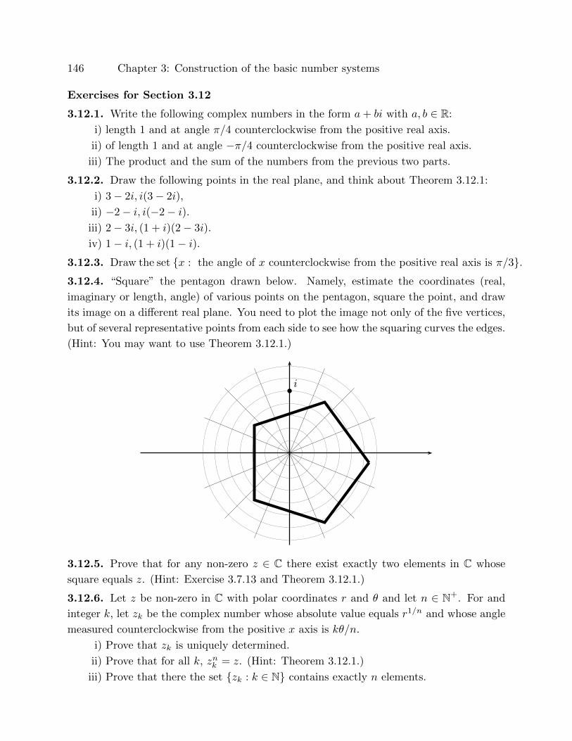
146 Chapter 3: Construction of the basic number systems
Exercises for Section 3.12
3.12.1. Write the following complex numbers in the form a+ bi with a, b ∈ R:
i) length 1 and at angle π/4 counterclockwise from the positive real axis.
ii) of length 1 and at angle −π/4 counterclockwise from the positive real axis.
iii) The product and the sum of the numbers from the previous two parts.
3.12.2. Draw the following points in the real plane, and think about Theorem 3.12.1:
i) 3− 2i, i(3− 2i),
ii) −2− i, i(−2− i).iii) 2− 3i, (1 + i)(2− 3i).
iv) 1− i, (1 + i)(1− i).3.12.3. Draw the set {x : the angle of x counterclockwise from the positive real axis is π/3}.3.12.4. “Square” the pentagon drawn below. Namely, estimate the coordinates (real,
imaginary or length, angle) of various points on the pentagon, square the point, and draw
its image on a different real plane. You need to plot the image not only of the five vertices,
but of several representative points from each side to see how the squaring curves the edges.
(Hint: You may want to use Theorem 3.12.1.)
� i
3.12.5. Prove that for any non-zero z ∈ C there exist exactly two elements in C whose
square equals z. (Hint: Exercise 3.7.13 and Theorem 3.12.1.)
3.12.6. Let z be non-zero in C with polar coordinates r and θ and let n ∈ N+. For and
integer k, let zk be the complex number whose absolute value equals r1/n and whose angle
measured counterclockwise from the positive x axis is kθ/n.
i) Prove that zk is uniquely determined.
ii) Prove that for all k, znk = z. (Hint: Theorem 3.12.1.)
iii) Prove that there the set {zk : k ∈ N} contains exactly n elements.

Section 3.13: Topology on the fields of real and complex numbers 147
3.13 Topology on the fields of real and complex numbers
When reading this section, absorb the following main points of topology: open ball,
open set, limit point, closed set. The main object of this section is to introduce limit points
of sets so that we can in subsequent chapters talk about limits of functions, sequences, and
series.
By a topology on a set we mean that some sets are declared open, subject to the
conditions that the empty set and the whole set have to be open, that arbitrary unions of
open sets be open, and that finite intersections of open sets be open. In any topology, the
complement of an open set is called closed, but a set may be neither open nor closed. A
topology can be imposed on any set, not just R or C, but we focus on these two cases, and
in fact we work only with the “standard”, or “Euclidean” topology.
Definition 3.13.1. Let F be R or C. Let a ∈ F and let r be a positive real number. An
open ball with center a and radius r is a set of the form
B(a, r) = {x ∈ F : |x− a| < r}.
An open set in F is any set that can be written as a union of open balls.
The following are both B(0, 1), but the left one is a ball in R and the right one is a
ball in C. Note that they are different: by definition the left set is an open subset of R,
but if you think of it as a subset of C, it is not open (see Exercise 3.13.1).
−1 10 −1 10
Examples 3.13.2.
(1) B(a, r) is open.
(2) F = ∪a∈FB(a, 1) is an open set.
(3) The empty set is an open set because it is vacuously a union of open sets (see
page 52).
(4) For real numbers a < b, the interval in R of the form (a, b) is an open set in Rbecause it is equal to B((a+ b)/2, (b− a)/2). The interval (a,∞) is open because
it equals ∪∞n=1B(a+ n, 1).
(5) The set A = {x ∈ C : 1 < Rex < 3 and 0.5 < Imx < 2} is open in C. Namely,
this set is the union ∪a∈AB(a,min{Re a− 1, 3− Re a, Im a− 0.5, 2− Im a})).

148 Chapter 3: Construction of the basic number systems
(6) The set A = {x ∈ C : Rex < 1 and Imx < 2} is open in C. Namely, this set is
the union ∪a∈AB(a,min{1− Re a, 2− Im a}).
Theorem 3.13.3. B(a, r) has infinitely many points.
Proof. For each integer n ≥ 2, a + r/n ∈ B(a, r). Since r > 0, these numbers are all
distinct. Since N0 is infinite, so is the set of all integers that are at least 2.
Example 3.13.4. Thus if A is an open subset of F , then either A is empty or A has
infinitely many points. In particular, {a} is not open.
Theorem 3.13.5. Let A be an open set and let a ∈ A. Then there exists r > 0 such that
B(a, r) ⊆ A.
Proof. Since A is open, it is a union of open balls. Thus a is an element of one such ball
B(b, s), with B(b, s) ⊆ A.
�
�
b
a
Since a ∈ B(b, s), we have that |a − b| < s, so that r =
s− |a− b| is a positive real number. (In the illustration, this is the
distance between a and the outside of the circle.) We claim that
B(a, r) ⊆ B(b, s). To prove this, let x ∈ B(a, r). Then |x − b| =
|x − a + a − b| ≤ |x − a| + |a − b| by the triangle inequality, and
since |x − a| < r = s − |a − b|, it means that |x − b| < s, so that
x ∈ B(b, s). This proves the claim, and hence it proves that B(a, r) ⊆ A.
Theorem 3.13.6. (Topology on F )
(1) ∅ and F are open.
(2) An arbitrary union of open sets is open.
(3) A finite intersection of open sets is open.
Proof. The empty set can be written as an empty union of open balls, so it is open
vacuously, and F = ∪a∈FB(a, 1), so that F is open. This proves (1).
Every open set is a union of open balls, and so the union of open sets is a union of
open balls, hence open. This proves (2).
Now let A1, . . . , An be open sets. Let a ∈ A1 ∩ · · · ∩ An. By Theorem 3.13.5, for
each k = 1, . . . , n, there exists rk > 0 such that B(a, rk) ⊆ Ak. Set r = min{r1, . . . , rn}.
Section 3.13: Topology on the fields of real and complex numbers 149
Then B(a, r) ⊆ ∩nk=1B(a, rk) ⊆ ∩nk=1Ak. Thus for each a ∈ ∩nk=1Ak there exists ra > 0
such that B(a, ra) ⊆ ∩nk=1Ak. It follows that
∩nk=1Ak = ∪a∈∩nk=1
AkB(a, ra).
This proves that ∩nk=1Ak is a union of open balls, so it is open.
An arbitrary intersection of open sets need not be open: ∩∞n=1B(a, 1/n) = {a}, which
is not open.
Definition 3.13.7. Let A be an arbitrary subset of F and a ∈ F (not necessarily in A).
We say that a is a limit point of A if for all real numbers s > 0, B(a, s) contains elements
of A different from a.
Examples 3.13.8.
(1) If A = {a}, then the set of limit points of A is the empty set.
(2) If A = Q, then the set of limit points of A is R.
(3) The set of limit points of ∅ is empty, the set of limit points of R is R, and the set
of limit points of C is C.
(4) The set of limit points of B(a, r) equals {x ∈ F : |x− a| ≤ r}.
Definition 3.13.9. A set A is a closed set if it contains all of its limit points.
Theorem 3.13.10. A is open if and only if F \A is closed.
Proof. Suppose that A is open. Let x ∈ A. By Theorem 3.13.5, there exists r > 0 such
that B(x, r) ⊆ A. Thus B(x, r)∩ (F \A) = ∅, so that x is not a limit point of F \A. Thus
no point of A is a limit point of F \ A, which proves that any limit points of F \ A are in
F \A. Thus F \A is closed.
Now suppose that F \ A is closed. Let x ∈ A. Since F \ A contains all of its limit
points, then x is not a limit point of F \ A. Thus by the definition of limit points, there
exists r > 0 such that B(x, r) ∩ (F \ A) is empty. This means that B(x, r) ⊆ A. Thus
A = ∪x∈AB(x, rx) for appropriate rx > 0, so that A is open.
The following is now almost immediate from previous results:
Theorem 3.13.11. (Topology on F )
(1) ∅, F are closed sets.
(2) Arbitrary intersections of closed sets are closed.
(3) Finite unions of closed sets are closed.
Proof. Exercise 2.1.8 proves that the union of the complements of two sets equals the
complement of the intersection and that the it was proved that the intersection of the
150 Chapter 3: Construction of the basic number systems
complements of two sets equals the complement of the union, and an equally easily proved
mathematical truth is the following generalization to possibly many more sets:
F \⋃k∈I
Ak =⋂k∈I
(F \Ak), F \⋂k∈I
Ak =⋃k∈I
(F \Ak).
With this, (2) and (3) follow from the last two theorems, and (1) is trivial.
Both ∅ and F are open and closed, and these turn out to be the only sets that are
both open and closed (see Exercise 3.13.2). Some sets are neither open nor closed (see
Exercise 3.13.1).
Exercises for Section 3.13
3.13.1. Let A be the open ball in R of radius 1 and centered at 0. Since R is a subset of
C, then A is also a subset of C. Prove that A is neither a closed nor an open subset of C.
3.13.2. Let F be either R or C, and let A be a subset of F that is both closed and open.
and let A be a closed and open subset of F . Prove that A = ∅ or A = F .
3.13.3. Prove that Q is neither an open nor a closed subset of R or C.
3.13.4. Sketch the following subsets of C. Determine their sets of limit points, and whether
the sets are open, closed, or neither: {x ∈ C : Imx = 0 and 0 < Rex < 1}, {x ∈ C : Imx =
0 and 0 ≤ Rex ≤ 1}, {x ∈ C : −2 ≤ Imx ≤ 2 and 0 ≤ Rex ≤ 1}, {x ∈ C : 2 ≤ Imx ≤−2 and 0 ≤ Rex ≤ 1}, {1/n : n ∈ N+}.
3.13.5. For each of the following intervals as subsets of R, determine the set of limit points,
and whether the set is open, closed, or neither in R:
(0, 1), [0, 1], [3, 5), [3,∞).
3.13.6. Let a be a limit point of a set A. Suppose that a set B contains A. Prove that a
is a limit point of B.
3.13.7. Give examples of sets A ⊆ B ⊆ C and a ∈ C such that a is a limit point of B but
not of A.
3.13.8. Let A be a subset of C all of whose elements are real numbers. Prove that every
limit point of A is a real number.
Section 3.14: The Heine-Borel theorem 151
3.14 The Heine-Borel theorem
Closed and bounded sets in C and R have many excellent properties – we will for
example see in Section 5.3 that when a good (say continuous) real-valued function has a
closed and bounded domain, then that function achieves a maximum and minimum value,
et cetera. The concept of uniform continuity (introduced in Section 5.5) needs the fairly
technical Heine-Borel theorems proved in this section.
Construction 3.14.1. (Halving closed and bounded subsets of R and quartering closed
and bounded subsets of C) Let A be a bounded subset of of R or of C, and let P be a
property that applies to subsets of A. Boundedness of A guarantees that A fits inside
a closed bounded rectangle R0 in C. If A is a subset of R, we take the “rectangle” R0
to have height zero. This rectangle can be halved lengthwise and crosswise to get four
equal closed subrectangles. In the next iteration we pick, if possible, one of these four
closed quarter subrectangles such that its intersection with A has property P . We call this
subrectangle R1, and note that the side lengths are half the side lengths in R0 (and so the
area of R1 is one quarter of the area of R0). In general, once we have Rn, we pick its closed
quarter subrectangle Rn+1 such that Rn+1 ∩ A has property P and the sides of Rn+1 are
half the lengths of the sides in Rn. Write Rn = [an, bn] × [cn, dn] for some real numbers
an ≤ bn and cn ≤ dn. By construction, for all n, bn − an = (b0 − a0)/2n, and
a0 ≤ a1 ≤ a2 ≤ · · · ≤ an ≤ · · · ≤ bn · · · ≤ b2 ≤ b1 ≤ b0.
This means that {a1, a2, a3, . . .} is a non-empty subset of R that is bounded above, so that
by the Least upper bound property/theorem (Theorem 3.8.5), a = sup{a1, a2, a3, . . .} is
a real number. By definition, a ≤ b1, b2, b3, . . .. Similarly, b = inf{b1, b2, b3, . . .} is a real
number that is greater than or equal to a. Suppose that a < b. Then by Exercise 3.8.3,
there exists a positive integer N such that 1/2N < (b−a)/(b0−a0). But aN ≤ a ≤ b ≤ bN ,
so that 0 ≤ b− a ≤ bN − aN = (b0 − a0)/2N < b− a, which contradicts trichotomy. Thus
a = b, i.e., we just proved that
sup{a1, a2, a3, . . .} = inf{b1, b2, b3, . . .}.
Similarly,
c = sup{c1, c2, c3, . . .} = inf{d1, d2, d3, . . .}.
This means that the intersection of all the Rn equals the set {a+ ci}, consisting of exactly
one complex number. By the shrinking property of the subrectangles, for every δ > 0 there
exists a positive integer N such that RN ∩A ⊆ B(a+ ci, δ).
In particular, “quartering” of the closed and bounded region (interval) A =
[a0, b0] ⊆ R, means halving the rectangle (interval), and the intersection of all the chosen
152 Chapter 3: Construction of the basic number systems
closed half-rectangles is a set with exactly one element. That element is in A, so a real
number.
Theorem 3.14.2. (The Heine-Borel theorem (in R, C)) Let A be a closed and
bounded subset of R or C. For each c ∈ A let δc be a positive number. Then there exists
a finite subset S of A such that A ⊆ ∪c∈SB(c, δc).
Proof. We declare that a subset B of A satisfies (property) P if there exists a finite subset
S of B such that B ⊆ ∪c∈SB(c, δc). We want to prove that A has P .
Suppose for contradiction that A does not have P . Since A is closed and bounded, it
fits inside a closed rectangle R0. With Construction 3.14.1, we construct iteratively nested
subrectangles R0 ⊇ R1 ⊇ R2 ⊇ · · ·. The quarter subrectangles are chosen so that each
Rn ∩ A does not have P . This is true if n = 0 by assumption. Suppose that Rn has been
chosen so that Rn∩A does not have P . If the intersection with A of each of the four quarter
subrectangles of Rn has P , i.e., if each of the four subrectangles (as in Construction 3.14.1)
intersected with A is contained in the union of finitely many balls B(c, δc), then Rn ∩A is
covered by finitely many such balls as well, which contradicts the assumption on Rn. Thus
it is possible to choose Rn+1 so that Rn+1 ∩A does not have P . By construction, ∩∞n=1Rncontains exactly one point. Let that point be x. Since each Rn ∩ A has infinitely many
points, x is a limit point of A, and since A is closed, necessarily x ∈ A.
By the shrinking sizes of the Rn, there exists a positive integer N such that Rn ⊆B(x, δx). But then Rn ∩A has P , which contradicts the construction. Thus A has P .
Theorem 3.14.3. Let A be a closed and bounded subset of R or C, and for each a ∈ Alet δa be a positive number. Then there exist a finite subset S of A and a positive real
number δ such that A ⊆ ∪c∈SB(c, δc) and such that for all x ∈ A there exists c ∈ S such
that B(x, δ) ⊆ B(c, δc).
Proof. By Theorem 3.14.2, there exists a finite subset S of A such that A ⊆ ∪c∈SB(c, δc/2).
Let δ = 12 min{δc : c ∈ S}. Since S is a finite set, δ is a positive real number.
Let x ∈ A. By the choice of S there exists c ∈ S such that x ∈ B(c, δc/2). Let
y ∈ B(x, δ). Then
|y − c| = |y − x+ x− c| ≤ |y − x|+ |x− c| < δ + δc/2 ≤ δc,
so that y ∈ B(c, δc). It follows that B(x, δ) ⊆ B(c, δc).
Exercises for Section 3.14
Section 3.14: The Heine-Borel theorem 153
3.14.1. Let A = {x ∈ R : 2 ≤ x ≤ 3}. Prove that A ⊆ ∪a∈AB(a, 1/a). Does there exist a
finite set S of A such that A ⊆ ∪a∈SB(a, 1/a). If yes, find it, if no, explain why not.
3.14.2. Let A = {1/n : n ∈ N+} ⊆ R. Prove that A ⊆ ∪a∈AB(a, a/3). Does there exist a
finite set S of A such that A ⊆ ∪a∈SB(a, a/3). Repeat with A = N+.
3.14.3. Let A be a closed and bounded subset of R or C. Let I be a set and for each
k ∈ I let Uk be an open subset of F . Suppose that A ⊆⋃k∈I Uk. Prove that there exists a
finite subset K of I such that A ⊆⋃k∈K Uk. (Hint: Prove that for each a ∈ A there exists
δa > 0 such that B(a, δa) is in some Uk. Apply Theorem 3.14.2.)
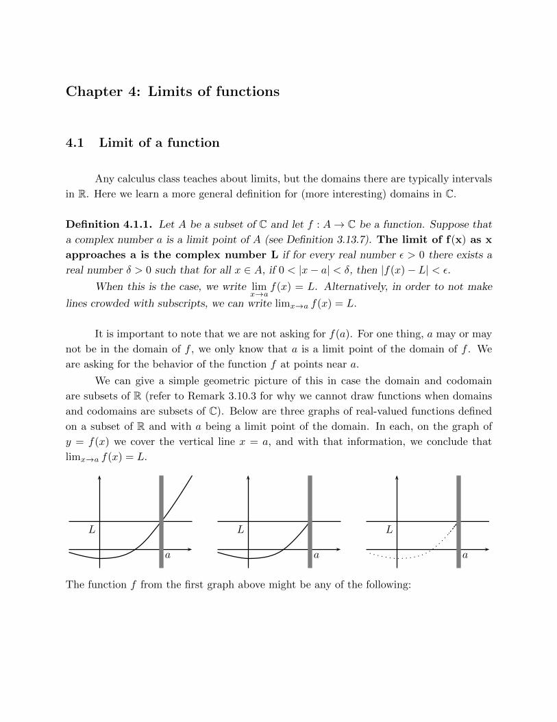
Chapter 4: Limits of functions
4.1 Limit of a function
Any calculus class teaches about limits, but the domains there are typically intervals
in R. Here we learn a more general definition for (more interesting) domains in C.
Definition 4.1.1. Let A be a subset of C and let f : A→ C be a function. Suppose that
a complex number a is a limit point of A (see Definition 3.13.7). The limit of f(x) as x
approaches a is the complex number L if for every real number ε > 0 there exists a
real number δ > 0 such that for all x ∈ A, if 0 < |x− a| < δ, then |f(x)− L| < ε.
When this is the case, we write limx→a
f(x) = L. Alternatively, in order to not make
lines crowded with subscripts, we can write limx→a f(x) = L.
It is important to note that we are not asking for f(a). For one thing, a may or may
not be in the domain of f , we only know that a is a limit point of the domain of f . We
are asking for the behavior of the function f at points near a.
We can give a simple geometric picture of this in case the domain and codomain
are subsets of R (refer to Remark 3.10.3 for why we cannot draw functions when domains
and codomains are subsets of C). Below are three graphs of real-valued functions defined
on a subset of R and with a being a limit point of the domain. In each, on the graph of
y = f(x) we cover the vertical line x = a, and with that information, we conclude that
limx→a f(x) = L.
a
L
a
L
a
L
The function f from the first graph above might be any of the following:

Section 4.1: Limit of a function 155
a
L
a
L
a
L
In an intuitive sense we are hoping that f(x) for x near a can predict a value of f
as we get arbitrarily close to a. For example, we may not be able to bring x to 0 Kelvin,
but if we can take measurements f(x) for x getting colder and colder, perhaps we can
theoretically predict what may happen at 0 Kelvin. But how believable is our prediction?
Perhaps for our theory to be satisfactory, we need to run experiments at temperatures x
that give us f(x) within ε = 10 of the predicted value. Or when instruments get better,
perhaps ε gets smaller, say one thousandth. Or a new material is discovered which allows us
to get ε even smaller. But no matter what ε is determined ahead of time, for the prediction
to be believable, we need to determine a range x within a δ of a but not equal to a, for
which the f -values are within the given ε of the prediction.
A graphical way of representing the epsilon-delta definition of limits for real-valued
functions with domains in R is as follows: For every positive ε there exists a positive δ such
that for all x in the domain with 0 < |x− a| < δ (the x 6= a in the vertical gray band), the
value of f(x) is within ε of L (in the horizontal grey band):
a
L+ εL
L− ε
a+ δa− δ
Clearly if ε gets smaller, δ has to get smaller too; and if ε gets larger, we may keep
the old δ.
While these pictures can help our intuition, they do not constitute a proof: the
definition is an algebraic formulation, and as such it requires algebraic proofs. In the rest
of the section we examine many examples algebraically, with the goal of mastering the
epsilon-delta proofs. But epsilon-delta proofs are time-consuming, so in the future we will
want to replace them with some shortcuts. We will have to prove that those shortcuts
are logically correct, and the proofs will require mastering abstract epsilon-delta proofs.
Naturally, before we can master abstract epsilon-delta proofs, we need to be comfortable
with epsilon-delta proofs on concrete examples. In short, in order to be able to avoid

156 Chapter 4: Limits of functions
epsilon-delta proofs, we have to master them. (Ha!)
Example 4.1.2. limx→3
(4x− 5) = 7.
Proof. The function that takes x to 4x − 5 is a polynomial function, so it is defined for
all complex numbers. Thus the domain of the function is C and 3 is a limit point of the
domain. Let ε > 0. [We are proving that for all real numbers ε > 0 something-
or-other holds. Recall that all proofs of this form start with “Let ε be
an arbitrary positive real number,” or abbreviated as we did. Now we have
to prove that the something-or-other holds. But this something-or-other
claims that there exists a real number δ > 0 with a certain property. Thus
we have to construct such a δ. In this first example I simply present a δ
that works, but in subsequent examples I show how to find a working δ. In
general, the proof should contain a specification of δ and a demonstration
that it works, but how one finds that δ is in general left to scratch work
or to inspiration. ] Set δ = ε/4. [Never mind how this magic ε/4 appears here;
wait until the next example where I present a process of finding δ.] Then
δ is a positive real number. [Sure! — Now we have to prove that for all x, if
0 < |x − 3| < δ, then |f(x) − L| < ε. The proof of “for all x . . .” starts with:]
Let x be an arbitrary complex number. [For this x we now have to prove that if
0 < |x − 3| < δ, then |f(x) − L| < ε. The proof of “If P then Q” starts with
“Assume P .”] Assume that 0 < |x − 3| < δ. [Now we have to prove Q, i.e., we
have to prove that |f(x) − L| = |(4x − 5) − 7| < ε. We do not simply write
“|(4x− 5)− 7| < ε” because we do not know that yet. We write the left side
of this inequality, and manipulate it – algebraically, often with triangle
inequalities and several steps, until we get < ε. ] Then
|(4x− 5)− 7| = |4x− 12|= 4|x− 3|< 4δ
= 4ε
4[Wasn’t ε/4 a clever choice of δ?]
= ε.
The commentary in the proof above is describing the thought process behind the
proof but need not and should not be written out in homework solutions. Below is a
homework-style solution:
Proof of Example 4.1.2 without the commentary: The function that takes x to 4x − 5 is
a polynomial function, so it is defined for all complex numbers. Thus the domain of the
function is C and 3 is a limit point of the domain. Let ε > 0. Set δ = ε/4. Then δ is a

Section 4.1: Limit of a function 157
positive real number. Let x be an arbitrary complex number. Assume that 0 < |x−3| < δ.
Then
|(4x− 5)− 7| = |4x− 12|= 4|x− 3|< 4δ
= 4ε
4= ε.
In the previous example δ appeared magically as ε/4, and it happened to be a positive
number depending on ε that made the limit proof work. Other numbers would have worked
as well, such as ε/5, or ε/(10000 + ε), and so on. For good style choose simple formulations
over complicated ones. If some positive number works as δ, so does any smaller positive
number, so there is no smallest possible δ and there are many different correct choices of δ.
It is not necessary to find the largest possible δ for a given ε, and it is not even necessary
to show how you derived or chose your δ. However, it is necessary to show that your pick
of δ does satisfy the rest of the defining property of limit.
Think through the comments in the previous paragraph on limx→4 5 = 5: any posi-
tive number works for δ.
In further examples we show all the necessary work for proofs of limits including how
to determine the δ. It is standard to use the proof-writing trick of partial filling-in: when
by the definition of limit it is time in the proof to declare what δ is, we typically write “Set
δ = ”, and in subsequent reasoning we fill in the underlined blank
with whatever restrictions seem necessary. Study the proofs below for how this is done,
but let me just say that each restriction puts an upper bound on δ, say bound δ above
by 1 and by ε2/4, and this is accomplished by filling in “Set δ = min{1, ε2/4 }”,
with room for possible further restrictions. (In Example 4.1.2 we only had one restriction,
namely δ ≤ ε/4, so that δ = min{ε/4} = ε/4.)
I find that the following two goals make these proofs more concrete and doable:
• Goal #1: Write |f(x)− L| as less than or equal to (something) times |x− a|,If f is a rational function, then |x− a| better be a factor of |f(x)− L|!• Goal #2: Find a positive constant upper bound B on the (something) found in
Goal #1. Then you make sure that δ ≤ ε/B.
You may want to keep these guidelines in mind as you read the proofs below.
158 Chapter 4: Limits of functions
Example 4.1.3. limx→−2
(4x2 − 5x+ 2) = 28.
Proof. The function that takes x to 4x2 − 5x + 2 is a polynomial function and it is
defined for all complex numbers. Thus −2 is a limit point of the domain. Let ε > 0.
Set δ = [δ to be determined still; the final write-up will
have this filled in, but we do not yet know δ.]. Then δ is a positive real number.
[Hoping, anyway.] Let x be any complex number. Suppose that 0 < |x+ 2| < δ. Then
|(4x2 − 5x+ 2)− 28| = |4x2 − 5x− 26| [Want Goal #1: x− a better be a factor.]
= |(x+ 2)(4x− 13)|= |4x− 13| · |x+ 2| [Goal #1 accomplished]
[Goal #2: we want to bound above the coefficient |4x − 13| of |x − a| by a
constant. But obviously |4x − 13| is not bounded above by a constant for
all x. So we need to make a restriction on δ: let’s make sure that δ is at
most 1 (or 2, or 15, it does not matter what positive number you pick in this
example). So on the δ line write: δ = min{1, }. This guarantees that
δ will be 1 or smaller, depending on what gets filled in after the comma.]
= |4(x+ 2− 2)− 13| · |x+ 2| (adding a clever zero)
= |4(x+ 2)− 21| · |x+ 2|
≤(|4(x+ 2)|+ 21
)· |x+ 2| (by the triangle inequality |a± b| ≤ |a|+ |b|)
< (4 · 1 + 21) · |x+ 2| (since |x+ 2| < δ ≤ 1)
= 25 · |x+ 2| [Goal #2 accomplished.]
[Now go back to specifying δ at the beginning of the proof by filling in
with: δ = min{1, ε/B}. This means that δ is the smaller of 1 and ε/B, and in
particular δ ≤ 1 and δ ≤ ε/B.]
< 25 · δ≤ 25 · ε/25
= ε.
The final version of the proof of limx→−2
(4x2 − 5x+ 2) = 28 then looks like this:
The function that takes x to 4x2 − 5x+ 2 is a polynomial function and it is defined
for all complex numbers. Thus −2 is a limit point of the domain. Let ε > 0. Set δ =
min{1, ε/25}. Then δ is a positive real number. Let x be any complex number. Suppose

Section 4.1: Limit of a function 159
that 0 < |x+ 2| < δ. Then
|(4x2 − 5x+ 2)− 28| = |4x2 − 5x− 26|= |(x+ 2)(4x− 13)|= |4x− 13| · |x+ 2|= |4(x+ 2− 2)− 13| · |x+ 2| (adding a clever zero)
= |4(x+ 2)− 21| · |x+ 2|≤ (|4(x+ 2)|+ 21) · |x+ 2|
(by the triangle inequality |a± b| ≤ |a|+ |b|)< (4 · 1 + 21) · |x+ 2| (since |x+ 2| < δ ≤ 1)
= 25 · |x+ 2|< 25 · δ≤ 25 · ε/25
= ε.
The next example has the same type of discovery work with fewer comments.
Example 4.1.4. limx→−1
(4/x2) = 4.
Proof. The function that takes x to 4/x2 is defined for all non-zero complex numbers, so
−1 is a limit point of the domain. Let ε > 0. Set δ = . Then δ is a positive
real number. Let x be any complex number that satisfies 0 < |x+ 1| < δ. Then
|4/x2 − 4| =∣∣∣∣4− 4x2
x2
∣∣∣∣= 4
∣∣∣∣ (1− x)(1 + x)
x2
∣∣∣∣= 4
∣∣∣∣1− xx2
∣∣∣∣ |1 + x| [Goal #1 accomplished: something times |x− a|.]
[Now we want the something 4(
1−xx2
)to be at most some constant. Certainly
if we allow x to get close to 0, then (1− x)/x2 will have a very large size,
so in order to find an upper bound, we need to make sure that x stays away
from 0. Since x is within δ of −1, in order to avoid 0 we need to make sure
that δ is strictly smaller than 1. For example, make sure that δ ≤ 0.4. Thus,
on the δ line write: δ = min{0.4, }.]
= 4
∣∣∣∣2− (x+ 1)
|x|2
∣∣∣∣ |1 + x| (by rewriting 1− x = 2− (x+ 1))

160 Chapter 4: Limits of functions
≤ 42 + |x+ 1|
x2|1 + x| (by the triangle inequality)
≤ 42.4
|x|2|1 + x| (since δ ≤ 0.4)
=9.6
|x+ 1− 1|2|1 + x| (by rewriting x = x+ 1− 1)
≤ 9.6
0.62|1 + x| (by the reverse triangle inequality because
|x+ 1− 1| ≥ 1− |x+ 1| > 1− δ ≥ 1− 0.4 = 0.6,
so that 1/|x+ 1− 1|2 < 1/0.62)
[On the δ-line now write: δ = min{0.4, 0.62ε/9.6}.]
<9.6
0.62δ
≤ 9.6
0.620.62ε/9.6
= ε.
And here is another example for good measure, with δ already filled in:
Example 4.1.5. limx→2i
4x3+x8x−i = −2.
Proof. The domain of 4x3+x8x−i consists of all complex numbers different from i/8, so 2i is a
limit point of the domain. Let ε > 0. Set δ = min{1, ε/9}. [It is so obvious that this
minimum of two positive numbers is positive that we skip the assertion “Thus
δ is a positive real number.” Do not omit the assertion or the checking of
its veracity for more complicated specifications of δ.] Let x be any complex
number different from i/8 such that 0 < |x−2i| < δ. [Here we merged: “Let x be any
complex number different from i/8. Let x satisfy 0 < |x − 2i| < δ.” into one
shorter and logically equivalent statement “Let x be any complex number
different from i/8 such that 0 < |x− 2i| < δ.”] Then∣∣∣∣4x3 + x
8x− i− (−2)
∣∣∣∣ =
∣∣∣∣4x3 + x
8x− i+ 2
∣∣∣∣=
∣∣∣∣4x3 + x+ 16x− 2i
8x− i
∣∣∣∣=
∣∣∣∣4x3 + 17x− 2i
8x− i
∣∣∣∣=
∣∣∣∣ (4x2 + 8ix+ 1)(x− 2i)
8x− i
∣∣∣∣=
∣∣∣∣ (4x2 + 8ix+ 1)
8x− i
∣∣∣∣ |x− 2i| (Goal #1: x− a is a factor.)

Section 4.1: Limit of a function 161
≤ |4x2|+ |8ix|+ 1
|8x− i||x− 2i| (by the triangle inequality)
≤ 4|(x− 2i+ 2i)|2 + 8|x− 2i+ 2i|+ 1
|8(x− 2i) + 15i||x− 2i|
≤ 4(|x− 2i|+ 2)2 + 8(|x− 2i|+ 2) + 1
−8|x− 2i|+ 15|x− 2i|
(by the triangle and reverse triangle inequalities)
≤ 4(1 + 2)2 + 8(1 + 2) + 1
−8 + 15|x− 2i| (since |x− 2i| < δ ≤ 1)
=61
7|x− 2i|
< 9δ
≤ 9ε/9
= ε.
The next example is of a limit is at a non-specific a.
Example 4.1.6. limx→a
(x2 − 2x) = a2 − 2a.
Proof. Any a is a limit point of the domain of the given polynomial function. Let ε > 0.
Set δ = min{1, ε/(1 + |2a− 2|)}. Let x satisfy 0 < |x− a| < δ. Then
|(x2 − 2x)− (a2 − 2a)| = |(x2 − a2)− (2x− 2a)| (by algebra)
= |(x+ a)(x− a)− 2(x− a)| (by algebra)
= |(x+ a− 2)(x− a)| (by algebra)
= |x+ a− 2| |x− a|= |(x− a) + 2a− 2| |x− a| (by adding a clever 0)
≤ (|x− a|+ |2a− 2|) |x− a| (by the triangle inequality)
≤ (1 + |2a− 2|) |x− a| (since |x− a| < δ ≤ 1)
< (1 + |2a− 2|)δ≤ (1 + |2a− 2|)ε/(1 + |2a− 2|)= ε.
Remark 4.1.7. Note that δ depends on ε and a, which are constants in the problem; δ is
not allowed to depend on x, as the definition goes:
“for all ε > 0 there exists δ > 0 such that for all x, etc”
so that x depends on δ, but δ does not depend on x.
By the definition of limits, δ is supposed to be a positive real number, not a function of x.
(See also Exercise 4.1.1.)
162 Chapter 4: Limits of functions
Remark 4.1.8. In all cases of rational functions, such as in examples above, Goal #1 is
to factor x− a from f(x)− L: if x− a is not a factor, check your limit or algebra for any
mistakes. In the next example, x− a is not a factor, but√x− a is.
Example 4.1.9. limx→3
√2x− 6 = 0.
Proof. The domain here is all x ≥ 3. So 3 is a limit point of the domain. Let ε > 0. Set
δ = ε2/2. Let x > 3 satisfy 0 < |x− 3| < δ. Then√
2x− 6 =√
2 ·√x− 3
<√
2 ·√δ (because
√is an increasing function)
=√
2 ·√ε2/2
= ε.
Often books consider the last example as a case of a one-sided limit (see definition
below) since we can only take the x from one side of 3. Our definition handles both-sided
and one-sided and all sorts of other limits with one simple notation, but we do have a use
for one-sided limits as well, so we define them next.
Definition 4.1.10. Let A ⊆ R, a ∈ R, L ∈ C, and f : A → C a function. Suppose that
a is a limit point of {x ∈ A : x > a} (resp. of {x ∈ A : x < a}). We say that the right-
sided (resp. left-sided) limit of f(x) as x approaches a is L if for every real number
ε > 0 there exists a real number δ > 0 such that for all x ∈ A, if 0 < x − a < δ (resp. if
0 < a − x < δ) then |f(x) − L| < ε. When this is the case, we write limx→a+ f(x) = L
(resp. limx→a− f(x) = L).
With this, Example 4.1.9 can be phrased as limx→3+
√2x− 6 = 0, and the proof goes
as follows: The domain A consists of all x ≥ 3, and 3 is a limit point of A∩{x : x > 3} = A.
Let ε > 0. Set δ = ε2/2. Let x satisfy 0 < x− 3 < δ. Then√
2x− 6 =√
2 ·√x− 3
<√
2 ·√δ
=√
2 ·√ε2/2
= ε.
Thus, the two proofs are almost identical. Note that limx→3−√
2x− 6 does not exist
because 3 is not the limit point of A ∩ {x ∈ R : x < 3} = ∅.One-sided limits can also be used in contexts where limx→a f(x) does not exist.
Below is one example.

Section 4.1: Limit of a function 163
Example 4.1.11. Let f : R → R be given by f(x) =
{x2 + 4, if x > 1;x− 2, if x ≤ 1.
Then
limx→1+ f(x) = 5, limx→1− f(x) = −1.
Proof. Let ε > 0.
Set δ = min{1, ε/3}. Let x satisfy 0 < x− 1 < δ. Then
|f(x)− 5| = |x2 + 4− 5| (since x > 1)
= |x2 − 1|= |(x+ 1)(x− 1)|< |x+ 1|δ (since x > 1, so x+ 1 is positive)
= |x− 1 + 2|δ (by adding a clever 0)
≤ (|x− 1|+ 2)δ (by the triangle inequality)
< (1 + 2)δ (since 0 < x− 1 < δ ≤ 1)
≤ 3ε/3
= ε.
This proves that limx→1+ f(x) = 5.
Set δ = ε. Let x satisfy 0 < 1− x < δ. Then
|f(x)− (−1)| = |x− 2 + 1| (since x < 1)
= |x− 1|< δ
= ε.
This proves that limx→1− f(x) = −3.
Exercises for Section 4.1
4.1.1. Below is an attempt at a “proof” that limx→3 x2 = 9. Explain how the two starred
steps below contain three mistakes.
Let ε > 0. Set δ =∗ ε/|x+ 3|. Then
|x2 − 9| = |x− 3| · |x+ 3|<∗ δ|x+ 3|= ε.
164 Chapter 4: Limits of functions
4.1.2. Fill in the blanks of the following proof that limx→2(x2 − 3x) = −2. Explain why
none of the inequalities can be changed into equalities.
so that 2 is a . Let ε > 0. Set δ = . Let x satisfy
0 < |x− 2| < δ. Then
|(x2 − 3x)− (−2)| =∣∣x2 − 3x+ 2
∣∣= |x− 1| |x− 2| (because )
= |x− 2 + 1| |x− 2| (by )
≤(|x− 2|+ 1
)|x− 2| (by )
< (3 + 1) |x− 2| (because )
< 4δ (because )
≤ 4ε
4(because )
= ε.
i) If the domain of this function is R as opposed to C, then |x− 2| < 4 can be shown
also with the following proof: Since |x− 2| < δ ≤ 3, then −3 < x− 2 < 3, so that
−2 < x − 1 < 4, which means that |x − 1| < 4. Say why this argument does not
work if the domain is C.
4.1.3. Determine the following limits and prove them with the epsilon-delta proofs.
i) limx→1
(x3 − 4).
ii) limx→2
1x .
iii) limx→3
x−4x2+2 .
iv) limx→4
√x+ 5.
v) limx→3
x2−9x−3 .
4.1.4. Rework Example 4.1.3 with choosing δ to be at most 2 rather than at most 1.
4.1.5. Let b ∈ C and f, g : C→ C with
f(x) =
{x3 − 4x2, if x 6= 5;b, if x = 5,
g(x) =
{x3 − 4x2, if x = 5;b, if x 6= 5.
Prove that the limit of f(x) as x approaches 5 is independent of b, but that the limit of
g(x) as x approaches 5 depends on b.
4.1.6. Suppose that a is a limit point of {x ∈ A : x > a} and of {x ∈ A : x < a}. Prove
that limx→a f(x) = L if and only if limx→a+ f(x) = L and limx→a− f(x) = L.
4.1.7. Suppose that a is a limit point of {x ∈ A : x > a} but not of {x ∈ A : x < a}.Prove that limx→a f(x) = L if and only if limx→a+ f(x) = L.
Section 4.2: When a number is not a limit 165
4.1.8. Prove that limx→a(mx+ l) = ma+ l, where m and l are constants.
4.1.9. Let f : R → R be given by f(x) = x|x| . Prove that limx→0+ f(x) = 1 and that
limx→0− f(x) = −1.
4.1.10. Find a function f : R→ R such that limx→0− f(x) = 2 and limx→0+ f(x) = −5.
4.1.11. Find a function f : R → R such that limx→0− f(x) = 2, limx→0+ f(x) = −5,
limx→1− f(x) = 3, and limx→1+ f(x) = 0. (Try to define such a function with fewest
possible words or symbols, but do use full grammatical sentences.)
4.2 When a number is not a limit
Recall that limx→a f(x) = L means that a is a limit point of the domain of f , and
that for all real numbers ε > 0 there exists a real number δ > 0 such that for all x in the
domain of f , if 0 < |x − a| < δ then |f(x) − L| < ε. [Think of limx→a f(x) = L as
statement P , a being a limit point of the domain as statement Q, and the
epsilon-delta part as statement R. By definition, P is logically the same as
the statement Q andR.]
Thus if limx→a f(x) 6= L, then either a is not a limit point of the domain of f or else
it is not true that for all real numbers ε > 0 there exists a real number δ > 0 such that for
all x in the domain of f , if 0 < |x− a| < δ then |f(x)− L| < ε. [This simply says that
notP is the same as ( notQ) or ( notR).]
In particular,
limx→a
f(x) 6= L and a is a limit point of the domain of f
means that it is not true that for all real numbers ε > 0 there exists a real number δ > 0
such that for all x in the domain of f , if 0 < |x− a| < δ then |f(x)− L| < ε. [This says
that ( notP ) andQ is the same as notR. You may want to write truth tables
for yourself.]
Negations of compound sentences, such as in the previous paragraph, are typically
hard to process and to work with in proofs. But by the usual negation rules of compound
statements (see chart on page 32), we successively rewrite this last negation into a form
that is easier to handle:
not(For all real numbers ε > 0 there exists a real number δ > 0
such that for all x in the domain of f , if 0 < |x − a| < δ
then |f(x)− L| < ε.)
[Negation of “For all z of some kind, property P holds” is “There is some z
of that kind for which P is false.” Hence the following rephrasing:]
166 Chapter 4: Limits of functions
= There exists a real number ε > 0 such that not(there exists a
real number δ > 0 such that for all x in the domain of f , if
0 < |x− a| < δ then |f(x)− L| < ε.)
[Negation of “There exists z of some kind such that property P holds” is
“For all z of that kind, P is false.” Hence the following rephrasing:]
= There exists a real number ε > 0 such that for all real numbers
δ > 0, not(for all x in the domain of f , if 0 < |x− a| < δ
then |f(x)− L| < ε.)
[Negation of “For all z of some kind, property P holds” is “There is some z
of that kind for which P is false.” Hence the following rephrasing:]
= There exists a real number ε > 0 such that for all real numbers
δ > 0, there exists x in the domain of f such that not(if
0 < |x− a| < δ then |f(x)− L| < ε.)
[Negation of “If P then Q” is “P and not Q.” Hence the following rephras-
ing:]
= There exists a real number ε > 0 such that for all real numbers
δ > 0, there exists x in the domain of f such that 0 <
|x− a| < δ and not(|f(x)− L| < ε.
)= There exists a real number ε > 0 such that for all real numbers
δ > 0, there exists x in the domain of f such that 0 <
|x− a| < δ and |f(x)− L| ≥ ε.
In summary, we just proved that:
Theorem 4.2.1. If a is a limit point of the domain of f , then limx→a f(x) 6= L means
that there exists a real number ε > 0 such that for all real numbers δ > 0, there exists x
in the domain of f such that 0 < |x− a| < δ and |f(x)− L| ≥ ε.
Example 4.2.2. The limit of x|x| as x approaches 0 does not exist. In other words, for all
complex numbers L, limx→0x|x| 6= L.
The domain of the function that takes x to x|x| is the set of all non-zero complex
numbers. For each non-zero x, x|x| is a complex number of length 1 and with the same
angle as x. Thus the image of this function is the unit circle in C. Note that it is possible
to take two non-zero x very close to 0 but at different angles so that their images on the
unit circle are far apart. This is a geometric reasoning why the limit cannot exist. Next
we give an epsilon-delta proof.
Proof. The domain of the function that takes x to x|x| is the set of all non-zero complex
numbers, so that 0 is a limit point of the domain. [Thus if the limit is not L, then
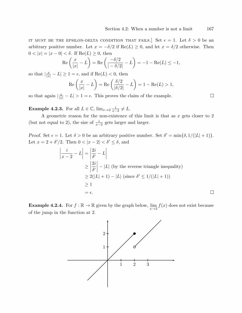
Section 4.2: When a number is not a limit 167
it must be the epsilon-delta condition that fails.] Set ε = 1. Let δ > 0 be an
arbitrary positive number. Let x = −δ/2 if Re(L) ≥ 0, and let x = δ/2 otherwise. Then
0 < |x| = |x− 0| < δ. If Re(L) ≥ 0, then
Re
(x
|x|− L
)= Re
(−δ/2| − δ/2|
− L)
= −1− Re(L) ≤ −1,
so that | x|x| − L| ≥ 1 = ε, and if Re(L) < 0, then
Re
(x
|x|− L
)= Re
(δ/2
|δ/2|− L
)= 1− Re(L) > 1,
so that again | x|x| − L| > 1 = ε. This proves the claim of the example.
Example 4.2.3. For all L ∈ C, limx→2i
x−2 6= L.
A geometric reason for the non-existence of this limit is that as x gets closer to 2
(but not equal to 2), the size of ix−2 gets larger and larger.
Proof. Set ε = 1. Let δ > 0 be an arbitrary positive number. Set δ′ = min{δ, 1/(|L|+ 1)}.Let x = 2 + δ′/2. Then 0 < |x− 2| < δ′ ≤ δ, and∣∣∣∣ i
x− 2− L
∣∣∣∣ =
∣∣∣∣2iδ′ − L∣∣∣∣
≥∣∣∣∣2iδ′∣∣∣∣− |L| (by the reverse triangle inequality)
≥ 2(|L|+ 1)− |L| (since δ′ ≤ 1/(|L|+ 1))
≥ 1
= ε.
Example 4.2.4. For f : R→ R given by the graph below, limx→2
f(x) does not exist because
of the jump in the function at 2.
1 2 3
1
2
168 Chapter 4: Limits of functions
Here is an epsilon-delta proof. Say that the limit exists. Call it L. Set ε = 14 . Let δ
be an arbitrary positive number. If L ≥ 32 , set x = 2 + min
{14 ,
δ2
}, and if L < 3
2 , set
x = 2−min{ 14 ,
δ2}. In either case,
0 < |x− 2| = min
{1
4,δ
2
}≤ δ
2< δ.
If L ≥ 32 , by our choice x = 2 + min{ 1
4 ,δ2}, so that f(x) = 1 + min{ 1
4 ,δ2} ≤ 1 + 1
4 ,
whence |f(x) − L| ≥ 14 = ε. Similarly, if L < 3
2 , by our choice x = 2 −min{ 14 ,
δ2}, so that
f(x) = 2 −min{ 14 ,
δ2} ≥ 2 − 1
4 = 1 + 34 , whence |f(x) − L| ≥ 1
4 = ε. Thus no L works, so
the limit of f(x) as x approaches 2 does not exist.
Exercises for Section 4.2
4.2.1. Prove that limx→3(3x− 4) 6= −3.
4.2.2. Prove that limx→1(x2 + 4) 6= −5.
4.2.3. Prove that limx→−3x−3x2−9 does not exist.
4.2.4. Prove that for all a ∈ R, limx→a f(x) does not exist, where f : R→ R is defined by
f(x) =
{1, if x is rational;0, if x is not rational.
4.2.5. Prove that limx→0(√x−√−x) does not exist. (Hint: The reason is different from
the reasons in other examples in this section.)
4.3 Limit theorems
While epsilon-delta proofs are a reliable method for proving limits, they do not help
in deciding what a limit may be. In this section we prove theorems that will efficiently
establish the limits for many functions. The proofs of these theorems require the epsilon-
delta machinery – as this is the definition of limits, but subsequent applications of these
theorems allow us to omit the time-consuming epsilon-delta proofs.
Theorem 4.3.1. If a limit exists, it is unique.
Proof. Suppose that both L1 and L2 are limits of f(x) as x approaches a.
First I give a FALSE proof: by assumption, L1 = limx→a f(x) = L2, so that by
transitivity of equality, L1 = L2. ×What makes this proof false is that the equal sign in “limx→a f(x) = L” signifies, at this
point, not numerical equality, but that a is a limit point of the domain of f and that for
Section 4.3: Limit theorems 169
every ε > 0 there exists δ > 0 such that for all x in the domain of f , if 0 < |x− a| < δ then
|f(x)− L| < ε. Thus, we need a proof that will use these definitions.
Real proof: Suppose that L1 and L2 are both limits. Let ε be an arbitrary positive
number. Then ε/2 is also positive, and by the definition of limits, for each i = 1, 2, there
exists δi > 0 such that for all x in the domain of f , if 0 < |x−a| < δi, then |f(x)−Li| < ε/2.
Set δ = min{δ1, δ2}. Then δ is a positive real number. Let x in the domain of f satisfy
0 < |x− a| < δ. Since a is a limit point of the domain, such x exists. Then
|L1 − L2| = |L1 − f(x) + f(x)− L2| (by adding a clever 0)
≤ |L1 − f(x)|+ |f(x)− L2| (by the triangle inequality)
< 2ε/2 (since δ ≤ δ1, δ2)
= ε,
which says that |L1 − L2| < ε. Since ε was arbitrary, an application of Theorem 2.10.4
gives that |L1 − L2| = 0, so that L1 − L2 = 0, and hence that L1 = L2.
(If in the definition of limx→a f(x) we did not require that a be a limit point of the
domain of f , then x as in the proof above would not exist for small δ, so any any complex
number L would vacuously satisfy the definition of limits. We would thus not be able
to guarantee that limits are unique. Perhaps the definition of limits is technical, but the
technicalities are there for a good reason.)
Theorem 4.3.2. Let a be a limit point of the domain of a function f with limx→a f(x) =
L. Suppose that L 6= 0. Then there exists δ > 0 such that for all x in the domain of f , if
0 < |x− a| < δ, then |f(x)| > |L|/2.
In particular, there exists δ > 0 such that for all x in the domain of f , if 0 < |x−a| <δ, then f(x) 6= 0.
Proof. Since |L|/2 > 0, there exists δ > 0 such that for all x in the domain of f , if
0 < |x− a| < δ, then |f(x)− L| < |L|/2. Hence by the reverse triangle inequality, for the
same x, |L|/2 > |f(x)−L| ≥ |L| − |f(x)|, so that by adding |f(x) + |L|/2 to both sides we
get that |f(x)| > |L|/2. In particular f(x) 6= 0.
The following theorem is very important, so study it carefully.
Theorem 4.3.3. Let A be the domain of f and g, and let a be a limit point of A, and let
c ∈ C. Suppose that limx→a f(x) and limx→a g(x) both exist. Then
(1) (Constant rule) limx→a
c = c.
(2) (Linear rule) limx→a
x = a.
(3) (Scalar rule) limx→a
cf(x) = c limx→a
f(x).
(4) (Sum/difference rule) limx→a
(f(x)± g(x)) = limx→a
f(x)± limx→a
g(x).
170 Chapter 4: Limits of functions
(5) (Product rule) limx→a
(f(x) · g(x)) = limx→a
f(x) · limx→a
g(x).
(6) (Quotient rule) If limx→a
g(x) 6= 0, then limx→a
f(x)
g(x)=
limx→a
f(x)
limx→a
g(x).
Proof. Both (1) and (2) were proved in Exercise 4.1.8.
Set L = limx→a f(x) and K = limx→a g(x).
(3) Let ε > 0. Then ε/(|c| + 1) is a positive number. (Note that we did not divide
by 0.) Since L = limx→a f(x), there exists δ > 0 such that for all x ∈ A, 0 < |x − a| < δ
implies that |f(x)− L| < ε/(|c|+ 1). Hence for the same x,
|cf(x)− cL| = |c| · |f(x)− L| < |c| · ε/(|c|+ 1) < ε,
which proves that limx→a cf(x) = cL = c limx→a f(x).
(4) Let ε > 0. Since L = limx→a f(x), there exists δ1 > 0 such that for all x ∈ A,
if 0 < |x − a| < δ1, then |f(x) − L| < ε/2. Similarly, since K = limx→a g(x), there exists
δ2 > 0 such that for all x ∈ A, if 0 < |x−a| < δ2, then |g(x)−L| < ε/2. Set δ = min{δ1, δ2}.Then δ is a positive number. Let x ∈ A satisfy 0 < |x− a| < δ. Then (4) follows from:
|(f(x)± g(x))− (L±K)| = |(f(x)− L)± (g(x)−K)| (by algebra)
≤ |f(x)− L|+ |g(x)−K| (by the triangle inequality)
< ε/2 + ε/2 (because 0 < |x− a| < δ ≤ δ1, δ2)
= ε.
(5) Let ε > 0. Then min{ε/(2|L|+ 2), 1}, min{ε/(2|K|+ 1), 1} are positive numbers.
Since L = limx→a f(x), there exists δ1 > 0 such that for all x ∈ A, if 0 < |x − a| < δ1,
then |f(x) − L| < min{ε/(2|K| + 1), 1}. Similarly, since K = limx→a g(x), there exists
δ2 > 0 such that for all x ∈ A, if 0 < |x − a| < δ2, then |g(x) − L| < ε/(2|L| + 2). Set
δ = min{δ1, δ2}. Then δ is a positive number. Let x ∈ A satisfy 0 < |x− a| < δ. Then by
the triangle inequality,
|f(x)| = |f(x)− L+ L| ≤ |f(x)− L|+ |L| < 1 + |L|,
and so
|f(x) · g(x)− L ·K| = |f(x) · g(x)− f(x)K + f(x)K − L ·K| (by adding a clever zero)
≤ |f(x) · g(x)− f(x)K|+ |f(x)K − L ·K| (by the triangle inequality)
= |f(x)| · |g(x)−K|+ |f(x)− L| · |K| (by factoring)
< (1 + |L|) · ε
2|L|+ 2+
ε
2|K|+ 1|K| (since δ ≤ δ1, δ2)
< ε/2 + ε/2
= ε.
Section 4.3: Limit theorems 171
(6) Let ε > 0. Since K 6= 0, by Theorem 4.3.2, there exists δ0 > 0 such that for all
x ∈ A, if 0 < |x− a| < δ0, then |g(x)| > |K|/2.
The numbers |K|ε/4, |K|2ε/(4|L|+ 1) are positive numbers. Since L = limx→a f(x),
there exists δ1 > 0 such that for all x ∈ A, if 0 < |x − a| < δ1, then |f(x) − L| < |K|ε/4.
Similarly, since K = limx→a g(x), there exists δ2 > 0 such that for all x ∈ A, if 0 < |x−a| <δ2, then |g(x)−L| < |K|2ε/(4|L|+1). Set δ = min{δ0, δ1, δ2}. Then δ is a positive number.
Let x ∈ A satisfy 0 < |x− a| < δ. Then∣∣∣∣f(x)
g(x)− L
K
∣∣∣∣ =
∣∣∣∣f(x)K − Lg(x)
Kg(x)
∣∣∣∣ (by algebra)
=
∣∣∣∣f(x)K − LK + LK − Lg(x)
Kg(x)
∣∣∣∣ (by adding a clever zero)
≤∣∣∣∣f(x)K − LK
Kg(x)
∣∣∣∣+
∣∣∣∣LK − Lg(x)
Kg(x)
∣∣∣∣ (by the triangle inequality)
=
∣∣∣∣f(x)− Lg(x)
∣∣∣∣+|L||K|
∣∣∣∣K − g(x)
g(x)
∣∣∣∣ (by factoring)
<|K|ε
4· 2
|K|+|L||K|
|K|2ε4|L|+ 1
· 2
|K|(since δ ≤ δ0, δ1, δ2)
< ε/2 + ε/2
= ε.
This proves (6) and thus the theorem.
Theorem 4.3.4. (Power rule for limits) Let n be a positive integer. If limx→a f(x) = L,
then limx→a f(x)n = Ln.
Proof. The case n = 1 is the assumption. Suppose that we know the result for n−1. Then
limx→a
f(x)n = limx→a
(f(x)n−1 · f(x)
)(by algebra)
= limx→a
(f(x)n−1
)· limx→a
(f(x)) (by the product rule)
= Ln−1 · L (by induction assumption)
= Ln.
So the result holds for n, and we are done by mathematical induction.
Theorem 4.3.5. (Polynomial function rule for limits) Let f be a polynomial func-
tion. Then for all complex (or real) a, limx→a f(x) = f(a).
Proof. Because f is a polynomial function, it can be written as
f(x) = c0 + c1x+ c2x2 + c3x
3 + · · ·+ cnxn

172 Chapter 4: Limits of functions
for some non-negative integer n and some constants c0, c1, . . . , cn. By the linear rule,
limx→a x = a. Hence by the power rule, for all i = 1, . . . , n, limx→a xi = ai. By the
constant rule, limx→a ci = ci, so that by the product rule limx→a cixi = cia
i. Hence by
repeating the sum rule,
limx→a
f(x) = limx→a
(c0 + c1x+ c2x
2 + · · ·+ cnxn)
= c0 +c1a+c2a2 + · · ·+cna
n = f(a).
Theorem 4.3.6. (Rational function rule for limits) Let f be a rational function.
Then for all complex (or real) a in the domain of f , limx→a f(x) = f(a).
Proof. Let a be in the domain of f . Write f(x) = g(x)/h(x) for some polynomial functions
g, h such that h(a) 6= 0. By Theorem 2.4.13, the domain of f is the set of all except finitely
many numbers, so that in particular a is a limit point of the domain. By the polynomial
function rule for limits, limx→a g(x) = g(a) and limx→a h(x) = h(a) 6= 0. Thus by the
quotient rule, limx→a f(x) = g(a)/h(a) = f(a).
Theorem 4.3.7. (Absolute value rule for limits) For all a ∈ C, limx→a |x| = |a|.
Proof. This function is defined for all complex numbers, and so every a ∈ C is a limit point
of the domain. Let ε > 0. Set δ = ε. Then for all x ∈ C, by the reverse triangle inequality,∣∣|x| − |a|∣∣ ≤ |x− a| < δ = ε.
Theorem 4.3.8. (Real and imaginary parts of limits) Let f : A → C be a func-
tion, let a be a limit point of A, and let L ∈ C. Then limx→a f(x) = L if and only if
limx→a Re f(x) = ReL and limx→a Im f(x) = ImL.
Proof. First suppose that limx→a f(x) = L. Let ε > 0. By assumption there exists δ > 0
such that for all x ∈ A, 0 < |x− a| < δ implies that |f(x)− L| < ε. Then for the same x,
|Re f(x)− ReL| = |Re(f(x)− L)| ≤ |f(x)− L| < ε,
and similarly | Im f(x) − ImL| < ε which proves that limx→a Re f(x) = ReL and
limx→a Im f(x) = ImL.
Now suppose that limx→a Re f(x) = ReL and limx→a Im f(x) = ImL. By the scalar
and sum rules in Theorem 4.3.3, and by the definition of real and imaginary parts,
limx→a
f(x) = limx→a
(Re f(x) + i Im f(x)) = limx→a
Re f(x) + i limx→a
Im f(x) = ReL+ i ImL = L.
Section 4.3: Limit theorems 173
Theorem 4.3.9. (The composite function theorem) Let h be the composition of
functions h = g◦f . Suppose that a is a limit point of the domain of g◦f , that limx→a
f(x) = L
and that limx→L
g(x) = g(L). Then limx→a
h(x) = limx→a
(g ◦ f)(x) = g(L).
Proof. Let ε > 0. Since limx→L
g(x) = g(L), there exists δ1 > 0 such that for all x in the
domain of g, if 0 < |x−a| < δ1 then |g(x)−g(L)| < ε. Since limx→a
f(x) = L, there exists δ > 0
such that for all x in the domain of f , if 0 < |x− a| < δ then |f(x)−L| < δ1. Thus for the
same δ, if x is in the domain of h and 0 < |x−a| < δ, then |h(x)−g(L)| = |g(f(x))−g(L)| < ε
because |f(x)− L| < δ1.
Perhaps the hypotheses on g in the theorem above seem overly restrictive, and you
think that the limit of g(x) as x approaches L need not be g(L) but an arbitrary K?
Consider the following example which shows that limx→a g(f(x)) then need not be K. Let
f(x) = 5 and g(x) =
{3, if x 6= 5;7, otherwise.
. Then
limx→a
f(x) = 5, limx→5
g(x) = 3, and limx→a
g(f(x)) = 7.
Theorem 4.3.10. Suppose that f, g : A→ R, that a is a limit point of A, that limx→a f(x)
and limx→a g(x) both exist, and that for all x ∈ A, f(x) ≤ g(x). Then
limx→a
f(x) ≤ limx→a
g(x).
Proof. Let L = limx→a
f(x), K = limx→a
g(x). Let ε > 0. By assumptions there exists δ > 0
such that for all x ∈ A, if 0 < |x− a| < δ, then |f(x)− L|, |g(x)−K| < ε/2. Then for the
same x,
K − L = K − g(x) + g(x)− f(x) + f(x)− L ≥ K − g(x) + f(x)− L≥ −|K − g(x) + f(x)− L|≥ −|K − g(x)| − |f(x)− L| (by the triangle inequality)
> −ε/2− ε/2 = −ε.
Since this is true for all ε > 0, by Theorem 2.10.4, K ≥ L, as desired.
Theorem 4.3.11. (The squeeze theorem) Suppose that f, g, h : A → R, that a is a
limit point of A, and that for all x ∈ A \ {a}, f(x) ≤ g(x) ≤ h(x). If limx→a f(x) and
limx→a h(x) both exist and are equal, then limx→a g(x) exists as well and
limx→a
f(x) = limx→a
g(x) = limx→a
h(x).
Proof. [If we knew that limx→a g(x) existed, then by the previous theorem,
limx→a f(x) ≤ limx→a g(x) ≤ limx→a h(x) = limx→a f(x) would give that the three
limits are equal. But we have yet to prove that limx→a g(x) exists.]

174 Chapter 4: Limits of functions
Let L = limx→a f(x) = limx→a h(x). Let ε > 0. Since limx→a f(x) = L, there
exists δ1 > 0 such that for all x, if 0 < |x − a| < δ1 then |f(x) − L| < ε. Similarly,
since limx→a h(x) = L, there exists δ2 > 0 such that for all x, if 0 < |x − a| < δ2 then
|h(x)− L| < ε. Now set δ = min{δ1, δ2}. Let x satisfy 0 < |x− a| < δ. Then
−ε < f(x)− L ≤ g(x)− L ≤ h(x)− L < ε,
where the first inequality holds because δ ≤ δ1, and the last inequality holds because δ ≤ δ2.
Hence −ε < g(x)− L < ε, which says that |g(x)− L| < ε, so that limx→a g(x) = L.
Exercises for Section 4.3
4.3.1. Determine the following limits by invoking appropriate results:
i) limx→2
(x3 − 4x− 27), limx→2
(x2 + 5).
ii) limx→2
(x3 − 4x− 27)3
(x2 + 5)2.
iii) limx→2
|x3 − 4x− 27|(x2 + 5)3
.
4.3.2. If limx→a
f(x) = L and limx→a
g(x) = K, prove that limx→a
(3f(x)2 − 4g(x)) = 3L2 − 4K.
4.3.3. Prove that limx→a
xn = an for any non-zero complex number a and any integer n.
4.3.4. Prove that for any positive real number a and any whole number n, limx→a
xn = an.
4.3.5. Prove that if limx→a f(x) = L, then limx→a |f(x)| = |L|. Give an example of a
function such that limx→a |f(x)| = |L| and limx→a f(x) does not exist.
4.3.6. Find functions f, g such that limx→a(f(x) + g(x)) exists but limx→a f(x) and
limx→a g(x) do not exist. Does this contradict the sum rule?
4.3.7. Find functions f, g such that limx→a(f(x)g(x)) exists but limx→a f(x) and
limx→a g(x) do not exist. Does this contradict the product rule?
4.3.8. Prove that limx→0
x|x| and lim
x→0
(1 − x
|x|)
do not exist, but that limx→0
(x|x| +
(1 − x
|x|))
does exist. Does this contradict the sum rule for limits? Justify.
4.3.9. Prove that limx→0
x|x| and lim
x→0
|x|x do not exist, but that lim
x→0
(x|x| ·
|x|x
)does exist. Does
this contradict the product rule for limits? Justify.
4.3.10. Let A ⊆ B ⊆ C, let a be a limit point of A, and let f : A→ C, g : B → C. Suppose
that for all x ∈ A\{x}, g(x) = f(x). Prove that if limx→a g(x) = L, then limx→a f(x) = L.
In particular, if a ∈ R is a limit point of A = B ∩ R and if limx→a g(x) = L, then the
restriction of g to A has the same limit point at a.
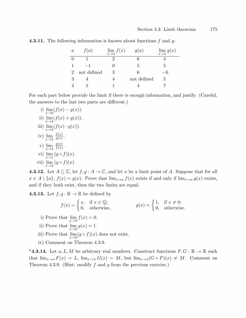
Section 4.3: Limit theorems 175
4.3.11. The following information is known about functions f and g:
a f(a) limx→a
f(x) g(a) limx→a
g(x)
0 1 2 6 4
1 −1 0 5 5
2 not defined 3 6 −6
3 4 4 not defined 5
4 5 1 4 7
For each part below provide the limit if there is enough information, and justify. (Careful,
the answers to the last two parts are different.)
i) limx→0
(f(x)− g(x)).
ii) limx→4
(f(x) + g(x)).
iii) limx→3
(f(x) · g(x)).
iv) limx→2
f(x)g(x) .
v) limx→4
g(x)f(x) .
vi) limx→1
(g ◦ f)(x).
vii) limx→4
(g ◦ f)(x).
4.3.12. Let A ⊆ C, let f, g : A→ C, and let a be a limit point of A. Suppose that for all
x ∈ A \ {a}, f(x) = g(x). Prove that limx→a f(x) exists if and only if limx→a g(x) exists,
and if they both exist, then the two limits are equal.
4.3.13. Let f, g : R→ R be defined by
f(x) =
{x, if x ∈ Q;0, otherwise,
g(x) =
{1, if x 6= 0;0, otherwise.
i) Prove that limx→0
f(x) = 0.
ii) Prove that limx→0
g(x) = 1.
iii) Prove that limx→0
(g ◦ f)(x) does not exist.
iv) Comment on Theorem 4.3.9.
*4.3.14. Let a, L,M be arbitrary real numbers. Construct functions F,G : R → R such
that limx→a F (x) = L, limx→LG(x) = M , but limx→a(G ◦ F )(x) 6= M . Comment on
Theorem 4.3.9. (Hint: modify f and g from the previous exercise.)

176 Chapter 4: Limits of functions
4.3.15. (Due to Jonathan Hoseana, “On zero-over-zero form limits of special type”, The
College Mathematics Journal 49 (2018), page 219.) ) Let f : [a, b] → R be a continuous
function. Let A be a subset of C, let a ∈ C be a limit point of A, and let f1, . . . , fn, g be
complex-valued functions defined on A such that for all k = 1, . . . , n, limx→a fk(x) = 1 and
limx→afk(x)−1g(x) exists. Prove that
limx→a
f1(x)f2(x) · · · fk(x)− 1
g(x)=
n∑k=1
limx→a
fk(x)− 1
g(x).
4.4 Infinite limits (for real-valued functions)
When the codomain of a function is a subset of an ordered field such as R, the values
of a function may grow larger and larger with no upper bound, or more and more negative
with no lower bound. In that case we may want to declare limit to be∞ or −∞. Naturally
both the definition and how we operate with infinite limits requires different handling.
Definition 4.4.1. Let A ⊆ C, f : A→ R a function, and a ∈ C. Suppose that a is a limit
point of A (and not necessarily in A).
We say that the limit of f(x) as x approaches a is ∞ if for every real number
M > 0 there exists a real number δ > 0 such that for all x ∈ A, if 0 < |x − a| < δ then
f(x) > M . We write this as limx→a
f(x) = limx→a f(x) = ∞. Similarly we say that the
limit of f(x) as x approaches a is −∞ if for every real number M < 0 there exists a
real number δ > 0 such that for all x ∈ A, if 0 < |x− a| < δ then f(x) < M . We write this
as limx→a
f(x) = limx→a f(x) = −∞.
The limit of f(x) as x approaches a from the right is −∞ if a is a limit point
of {x ∈ A : x > a}, and if for every real number M < 0 there exists a real number δ > 0
such that for all x ∈ A, if 0 < x − a < δ then f(x) < M . This is written as limx→a+
f(x)
= limx→a+ f(x) = −∞.
It is left to the reader to spell out the definitions of the following:
limx→a+
f(x) =∞, limx→a−
f(x) =∞, limx→a−
f(x) = −∞.
Note that we cannot use epsilon-delta proofs: no real numbers are within ε of infinity.
So instead we approximate infinity with huge numbers. In fact, infinity stands for that thing
which is larger than any real number. Thus for all M we can find x near a with f(x) > M
is simply saying that we can take f(x) arbitrarily large, which is more succinctly expressed
as saying that f(x) goes to ∞. (As far as many applications are concerned, a real number
larger than the number of atoms in the universe is as close to infinity as realistically possible,
but for proofs, the number of atoms in the universe is not large enough.)
Section 4.4: Infinite limits (for real-valued functions) 177
Example 4.4.2. limx→01|x|2 =∞.
Proof. 0 is a limit point of the domain (in the field of real or complex numbers) of the
function that takes x to 1/|x|2. Let M be a positive real number. Set δ = 1/√M . Let x
satisfy 0 < |x− 0| < δ, i.e., let x satisfy 0 < |x| < δ. Then
1
|x|2>
1
δ2(because 0 < |x| < δ)
= M.
Example 4.4.3. limx→5+x+2x2−25 =∞.
Proof. Certainly 5 is the limit point of the domain of the given function. Let M > 0. Set
δ = min{1, 711M }. Let x satisfy 0 < x− 5 < δ. Then
x+ 2
x2 − 25>
5 + 2
x2 − 25(because x > 5 and x2 − 25 > 0)
=7
(x+ 5)· 1
x− 5(by algebra)
>7
11· 1
x− 5(because 0 < x− 5 < δ ≤ 1, so 0 < x+ 5 < 11, and x− 5 > 0)
>7
11· 1
δ(because 0 < x− 5 < δ)
≥ 7
11· 1
711M
(because δ ≤ 711M , so 1/δ ≥ 1/( 7
11M ))
= M.
Example 4.4.4. limx→0+1x =∞.
Proof. Let M > 0. Set δ = 1/M . Then for all x with 0 < x− 0 < δ, 1x > 1/δ = M .
Example 4.4.5. limx→0−1x = −∞.
Proof. Let M < 0. Set δ = −1/M . Then δ is a positive number. Then for all x with
0 < 0− x < δ,1
x< −1/δ = M.
Example 4.4.6. We conclude that limx→01x cannot be a real number, and it cannot be
either ∞ or −∞. Thus limx→01x does not exist.
The following theorem is straightforward to prove, and so it is left for the exercises.
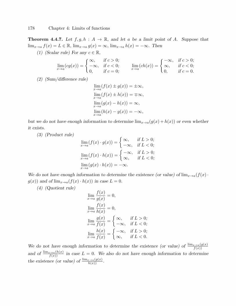
178 Chapter 4: Limits of functions
Theorem 4.4.7. Let f, g, h : A → R, and let a be a limit point of A. Suppose that
limx→a f(x) = L ∈ R, limx→a g(x) =∞, limx→a h(x) = −∞. Then
(1) (Scalar rule) For any c ∈ R,
limx→a
(cg(x)) =
{∞, if c > 0;−∞, if c < 0;0, if c = 0;
limx→a
(ch(x)) =
{−∞, if c > 0;∞, if c < 0;0, if c = 0.
(2) (Sum/difference rule)
limx→a
(f(x)± g(x)) = ±∞,
limx→a
(f(x)± h(x)) = ∓∞,
limx→a
(g(x)− h(x)) =∞,
limx→a
(h(x)− g(x)) = −∞,
but we do not have enough information to determine limx→a(g(x) +h(x)) or even whether
it exists.
(3) (Product rule)
limx→a
(f(x) · g(x)) =
{∞, if L > 0;−∞, if L < 0;
limx→a
(f(x) · h(x)) =
{−∞, if L > 0;∞, if L < 0;
limx→a
(g(x) · h(x)) = −∞.
We do not have enough information to determine the existence (or value) of limx→a(f(x) ·g(x)) and of limx→a(f(x) · h(x)) in case L = 0.
(4) (Quotient rule)
limx→a
f(x)
g(x)= 0,
limx→a
f(x)
h(x)= 0,
limx→a
g(x)
f(x)=
{∞, if L > 0;−∞, if L < 0;
limx→a
h(x)
f(x)=
{−∞, if L > 0;∞, if L < 0.
We do not have enough information to determine the existence (or value) of limx→a(g(x)f(x))
and of limx→a(h(x)f(x)) in case L = 0. We also do not have enough information to determine
the existence (or value) of limx→a(g(x)h(x)) .

Section 4.4: Infinite limits (for real-valued functions) 179
Example 4.4.8. Define g, h1, h2, h3, h4 : R \ {0} → R by g(x) = 1/x2, h1(x) = −1/x2,
h2(x) = 17 − 1/x2, h3(x) = −1/x2 − 1/x4, h4(x) = −1/x2 − 1/x3. We have seen that
limx→0 g(x) = ∞, and similarly that limx→0 h1(x) = limx→0 h2(x) = limx→0 h3(x) =
limx→0 h4(x) = −∞. However,
limx→0
(g(x) + h1(x)) = limx→0
0 = 0,
limx→0
(g(x) + h2(x)) = limx→0
17 = 17,
limx→0
(g(x) + h3(x)) = limx→0
(−1/x4) = −∞,
but limx→0(g(x) + h4(x)) = limx→0(−1/x3) does not exist. This justifies the “not enough
information” line in the sum/difference rule in Theorem 4.4.7.
Other “not enough information” lines are left for the exercises.
Distinguish between the scalar and the product rules: when limx→a f(x) = 0, if f is
a constant function, then limx→a(f(x)g(x)) = 0, but if f is not a constant function, then
we do not have enough information for limx→a(f(x)g(x)) = 0.
Exercises for Section 4.4
4.4.1. Give definitions for the following limits.
i) limx→a+ f(x) =∞.
ii) limx→a− f(x) =∞.
iii) limx→a− f(x) = −∞.
4.4.2. Prove that limx→0+1√x
=∞.
4.4.3. Prove that limx→0−1x3 = −∞.
4.4.4. This is about Theorem 4.4.7. Prove the scalar rule, the sum/difference rule, the
product rule, and the quotient rule.
4.4.5. Let g(x) = 1/x2, f1(x) = x3, f2(x) = x2, f3(x) = 17x2, f4(x) = x. It is easy to see
that limx→0 g(x) =∞, limx→0 f1(x) = limx→0 f2(x) = limx→0 f3(x) = limx→0 f4(x) = 0.
i) Compute the limits limx→0(f1(x)g(x)), limx→0(f2(x)g(x)), limx→0(f3(x)g(x)),
limx→0(f4(x)g(x)).
ii) Justify the first “not enough information” in the product rule in Theorem 4.4.7.
iii) Justify the second “not enough information” in the product rule in Theorem 4.4.7.
4.4.6. Justify the three “not enough information” in the quotient rule in Theorem 4.4.7.
(Hint: Study the previous exercise.)

180 Chapter 4: Limits of functions
4.5 Limits at infinity
Definition 4.5.1. Let a ∈ R and L ∈ C.
For f : (a,∞) → C, we say that limx→∞ = L if for every ε > 0 there exists a real
number N > 0 such that for all x > N , |f(x)− L| < ε.
For f : (−∞, a)→ C, we say that limx→−∞ = L if for every ε > 0 there exists a real
number N < 0 such that for all x < N , |f(x)− L| < ε.
Below we switch to real-valued functions.
For f : (a,∞)→ R, we say that limx→∞ =∞ if for every M > 0 there exists a real
number N > 0 such that for all x > N , f(x) > M . We say that limx→∞ = −∞ if for every
M < 0 there exists a real number N > 0 such that for all x > N , f(x) < M .
For f : (−∞, a) → R, we say that limx→−∞ = ∞ if for every M > 0 there exists a
real number N < 0 such that for all x < N , f(x) > M . We say that limx→−∞ = −∞ if
for every M < 0 there exists a real number N < 0 such that for all x < N , f(x) < M .
Example 4.5.2. limx→∞(x5 − 16x4) =∞.
Proof. Let M > 0. Set N = max{17,M1/4}. Then for all x > N ,
x5 − 16x4 = x4(x− 16)
≥ x4 (because x > N ≥ 17)
> N4 (because x > N)
≥ (M1/4)4 (because N ≥M1/4)
= M.
Example 4.5.3. limx→∞x5−16x4
x5+4x2 = 1.
Proof. Let ε > 0. Set N = max{1, 20/ε}. Then for all x > N ,∣∣∣∣x5 − 16x4
x5 + 4x2− 1
∣∣∣∣ =
∣∣∣∣x5 − 16x4 − x5 − 4x2
x5 + 4x2
∣∣∣∣=
∣∣∣∣−16x4 − 4x2
x5 + 4x2
∣∣∣∣=
∣∣∣∣16x4 + 4x2
x5 + 4x2
∣∣∣∣=
16x4 + 4x2
x5 + 4x2(because x > N ≥ 0)
≤ 16x4 + 4x2
x5(because x5 + 4x2 ≥ x5 > 0)
≤ 16x4 + 4x4
x5(because x > N ≥ 1 so that x2 < x4)

Section 4.5: Limits at infinity 181
=20x4
x5
=20
x
<20
N(because x > N)
≤ 20
20/ε(because N ≥ 20/ε)
= ε.
Exercises for Section 4.5
4.5.1. Prove that limx→∞(x2 − x) =∞ and that limx→−∞(x2 − x) =∞.
4.5.2. Prove that limx→∞(x3 − x) =∞ and that limx→−∞(x3 − x) = −∞.
4.5.3. Is there a limit rule of the following form: If limx→∞ f(x) =∞ and limx→∞ g(x) =
∞, then limx→∞(f(x)− g(x)) can be determined?
4.5.4. Prove the following limits:
i) limx→∞3x2−4x+1
2x2+2 = 3/2.
ii) limx→∞3x3−4x+1
2x2+2 =∞.
iii) limx→∞3x2−4x+1
2x3+2 = 0.
iv) limx→∞√
9x2+4x+2 = 3.
v) limx→−∞√
9x2+4x+2 = −3.
4.5.5. For which rational functions f does limx→∞ f(x) = 0 hold? Justify.
4.5.6. For which rational functions f does limx→∞ f(x) exist and is not ±∞? Justify.
4.5.7. Let f : (a,∞) → C and L ∈ C. Prove that limx→∞ f(x) = L if and only if
limx→∞Re f(x) = ReL and limx→∞ Im f(x) = ImL.
4.5.8. Let f : (−∞, b) → C and L ∈ C. Prove that limx→−∞ f(x) = L if and only if
limx→−∞Re f(x) = ReL and limx→−∞ Im f(x) = ImL.
Chapter 5: Continuity
Continuous functions from an interval in R to R are the ones that we can graph with-
out any holes or jumps, i.e., without lifting the pencil from the paper, so the range of such
functions is an interval in R as well. We make this more formal below, and not just for func-
tions with domains and codomains in R. The formal definition involves limits of functions.
All the hard work for that was already done in Chapter 4, so this chapter, after absorbing
the definition, is really straightforward. The big new results are the Intermediate value
theorem and the Extreme value theorem for real-valued functions (Section 5.3), existence
of radical functions (Section 5.4), and the new notion of uniform continuity (Section 5.5).
5.1 Continuous functions
Definition 5.1.1. A function f : A→ B is continuous at a ∈ A if for all real numbers
ε > 0 there exists a real number δ > 0 such that for all x ∈ A, |x − a| < δ implies that
|f(x) − f(a)| < ε. We say that f is continuous if f is continuous at all points in its
domain.
Much of the time for us A is an interval in R, a rectangle in C, or B(a, r) in R or C,
et cetera. In the more general case, A may contain a point a that is not a limit point of A.
Theorem 5.1.2. Let f : A→ B be a function and a ∈ A.
(1) If a is not a limit point of A, then f is continuous at a.
(2) If a is a limit point of A, then f is continuous at a if and only if limx→a f(x) = f(a).
Proof. In the first case, there exists δ > 0 such that B(a, δ)∩A = {a}. Thus by definition,
the only x ∈ A with |x− a| < δ is x = a, whence |f(x)− f(a)| = 0 is strictly smaller than
an arbitrary positive ε. Thus f : A→ B is continuous at a.
Now assume that a is a limit point of A. Suppose that f is continuous at a. We need
to prove that limx→a f(x) = f(a). Let ε > 0. Since f is continuous at a, there exists δ > 0
such that for all x ∈ A, if |x− a| < δ, then |f(x)− f(a)| < ε. Hence for all 0 < |x− a| < δ,
|f(x)− f(a)| < ε, and since a is a limit point of A, this proves that limx→a f(x) = f(a).
Finally suppose that limx→a f(x) = f(a). We need to prove that f is continuous at
a. Let ε > 0. By assumption there exists δ > 0 such that for all x ∈ A, if 0 < |x− a| < δ
then |f(x) − f(a)| < ε. If x = a, then |f(x) − f(a)| = 0 < ε, so that for all x ∈ A, if
|x− a| < δ, then |f(x)− f(a)| < ε. Thus f is continuous at a.

Section 5.1: Continuous functions 183
The next theorem is an easy application of Theorems 4.3.3, 4.3.4, 4.3.5, 4.3.6, 4.3.7,
4.3.8, and 4.3.9, at least when the points in question are limit points of the domain. When
the points in question are not limit points of the domain, the results below need somewhat
different but still easy proofs.
Theorem 5.1.3. We have:
(1) (Constant rule) Constant functions are continuous (at all real/complex numbers).
(2) (Linear rule) The function f(x) = x is continuous (at all real/complex numbers).
(3) (Absolute value rule) The function f(x) = |x| is continuous (at all real/complex
numbers).
(4) (Polynomial function rule) Polynomial functions are continuous (at all real/complex
numbers).
(5) (Rational function rule) Rational functions are continuous (at all points in the
domain).
(6) (Real and imaginary parts) f is continuous at a if and only if Re f and Im f are
continuous at a.
Suppose that f : A→ C is continuous at a ∈ A. Then
(7) (Scalar rule) For any c ∈ C, cf is continuous at a.
(8) (Power rule) For any positive integer n, the function that takes x to (f(x))n is
continuous at a.
(9) (The composite function rule) If g is continuous at f(a), then g ◦ f is continuous
at a.
(10) (The composite power rule) If f is composable with itself i.e., if the range of f is
a subset of the domain of f , then fn = f ◦ f ◦ · · · ◦ f is continuous at a. (Example
of a function that is not composable with itself: f(x) = lnx.)
(11) (Restriction rule) For any subset B of A that contains a and in which a is a limit
point, the restriction of f to B is continuous at a. In other words, if g : B → C is
defined as g(x) = f(x) for all x ∈ B, then g is continuous at a. (Such g is called
the restriction of f to B. By this rule and by (1), the constant functions with
domain a sub-interval in R are continuous.)
Now suppose that f, g : A→ C, and that f and g are continuous at a ∈ A. Then
(12) (Sum/difference rule) f + g and f − g are continuous at a.
(13) (Product rule) f · g is continuous at a.
(14) (Quotient rule) If g(a) 6= 0, then f/g is continuous at a.
The theorem covers many continuous functions, but the following function for exam-
ple has to be verified differently.
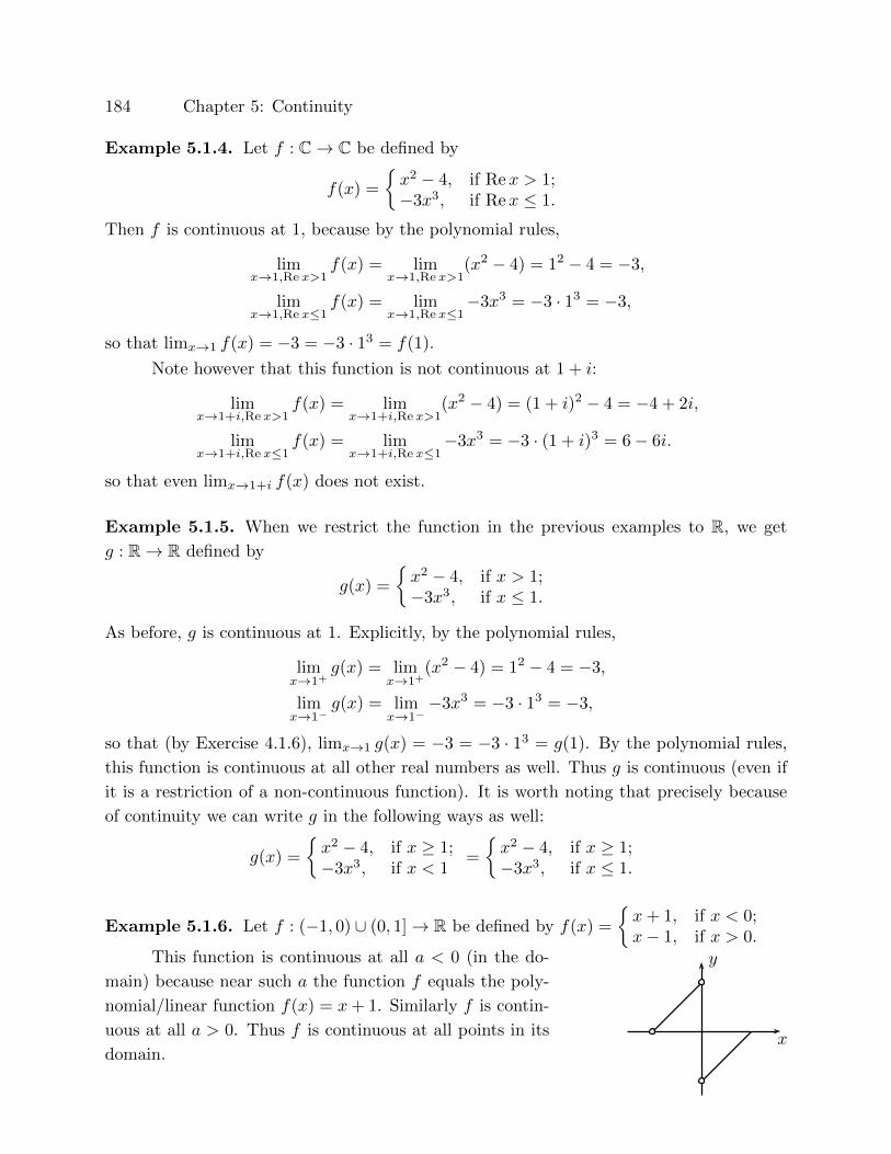
184 Chapter 5: Continuity
Example 5.1.4. Let f : C→ C be defined by
f(x) =
{x2 − 4, if Rex > 1;−3x3, if Rex ≤ 1.
Then f is continuous at 1, because by the polynomial rules,
limx→1,Re x>1
f(x) = limx→1,Re x>1
(x2 − 4) = 12 − 4 = −3,
limx→1,Re x≤1
f(x) = limx→1,Re x≤1
−3x3 = −3 · 13 = −3,
so that limx→1 f(x) = −3 = −3 · 13 = f(1).
Note however that this function is not continuous at 1 + i:
limx→1+i,Re x>1
f(x) = limx→1+i,Re x>1
(x2 − 4) = (1 + i)2 − 4 = −4 + 2i,
limx→1+i,Re x≤1
f(x) = limx→1+i,Re x≤1
−3x3 = −3 · (1 + i)3 = 6− 6i.
so that even limx→1+i f(x) does not exist.
Example 5.1.5. When we restrict the function in the previous examples to R, we get
g : R→ R defined by
g(x) =
{x2 − 4, if x > 1;−3x3, if x ≤ 1.
As before, g is continuous at 1. Explicitly, by the polynomial rules,
limx→1+
g(x) = limx→1+
(x2 − 4) = 12 − 4 = −3,
limx→1−
g(x) = limx→1−
−3x3 = −3 · 13 = −3,
so that (by Exercise 4.1.6), limx→1 g(x) = −3 = −3 · 13 = g(1). By the polynomial rules,
this function is continuous at all other real numbers as well. Thus g is continuous (even if
it is a restriction of a non-continuous function). It is worth noting that precisely because
of continuity we can write g in the following ways as well:
g(x) =
{x2 − 4, if x ≥ 1;−3x3, if x < 1
=
{x2 − 4, if x ≥ 1;−3x3, if x ≤ 1.
Example 5.1.6. Let f : (−1, 0) ∪ (0, 1]→ R be defined by f(x) =
{x+ 1, if x < 0;x− 1, if x > 0.
x
yThis function is continuous at all a < 0 (in the do-
main) because near such a the function f equals the poly-
nomial/linear function f(x) = x+ 1. Similarly f is contin-
uous at all a > 0. Thus f is continuous at all points in its
domain.
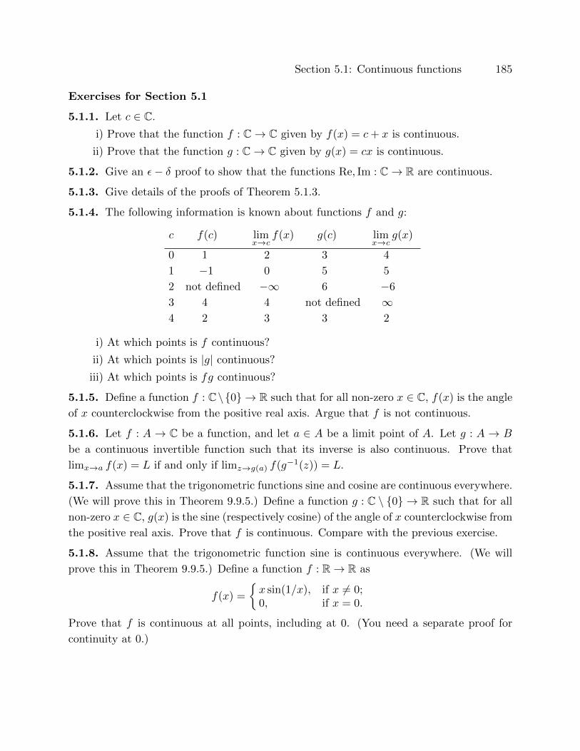
Section 5.1: Continuous functions 185
Exercises for Section 5.1
5.1.1. Let c ∈ C.
i) Prove that the function f : C→ C given by f(x) = c+ x is continuous.
ii) Prove that the function g : C→ C given by g(x) = cx is continuous.
5.1.2. Give an ε− δ proof to show that the functions Re, Im : C→ R are continuous.
5.1.3. Give details of the proofs of Theorem 5.1.3.
5.1.4. The following information is known about functions f and g:
c f(c) limx→c
f(x) g(c) limx→c
g(x)
0 1 2 3 4
1 −1 0 5 5
2 not defined −∞ 6 −6
3 4 4 not defined ∞4 2 3 3 2
i) At which points is f continuous?
ii) At which points is |g| continuous?
iii) At which points is fg continuous?
5.1.5. Define a function f : C\{0} → R such that for all non-zero x ∈ C, f(x) is the angle
of x counterclockwise from the positive real axis. Argue that f is not continuous.
5.1.6. Let f : A → C be a function, and let a ∈ A be a limit point of A. Let g : A → B
be a continuous invertible function such that its inverse is also continuous. Prove that
limx→a f(x) = L if and only if limz→g(a) f(g−1(z)) = L.
5.1.7. Assume that the trigonometric functions sine and cosine are continuous everywhere.
(We will prove this in Theorem 9.9.5.) Define a function g : C \ {0} → R such that for all
non-zero x ∈ C, g(x) is the sine (respectively cosine) of the angle of x counterclockwise from
the positive real axis. Prove that f is continuous. Compare with the previous exercise.
5.1.8. Assume that the trigonometric function sine is continuous everywhere. (We will
prove this in Theorem 9.9.5.) Define a function f : R→ R as
f(x) =
{x sin(1/x), if x 6= 0;0, if x = 0.
Prove that f is continuous at all points, including at 0. (You need a separate proof for
continuity at 0.)
186 Chapter 5: Continuity
5.1.9. Assume that the trigonometric function sine is continuous everywhere. (We will
prove this in Theorem 9.9.5.) Define a function f : R→ R as
f(x) =
{sin(1/x), if x 6= 0;0, if x = 0.
i) Is f continuous at 0? Prove or disprove.
ii) Prove that f is continuous at all other points.
5.1.10. Let f : R→ R be given by f(x) =
{x, if x is rational;0, otherwise.
i) Prove that f is continuous at 0.
ii) Prove that f is not continuous anywhere else.
*5.1.11. (The Thomae function, also called the popcorn function, the raindrop function,
and more) Let f : R→ R be defined as
f(x) =
{1q , if x = p
q , where p ∈ Z and q ∈ N+ have only 1 as a common factor;
0, if x is irrational.
i) Prove that f is not continuous at any rational number.
ii) Prove that f is continuous at all irrational numbers.
The exercises below modify the definition of continuity to get very different types of func-
tions. – The moral is that the order of quantifiers and implications is very important!
5.1.12. (This is from page 1177 of the Edward Nelson’s article “Internal set theory: a new
approach to nonstandard analysis.” Bull. Amer. Math. Soc. 83 (1977), no. 6, 1165–1198.)
A function f : A→ B is suounitnoc at a ∈ A if for all real numbers ε > 0 there exists a
real number δ > 0 such that for all x ∈ A, |x− a| < ε implies that |f(x)− f(a)| < δ.
i) Prove that if f is suounitnoc at some a ∈ A, it is suounitnoc at every b ∈ A.
ii) Let f : R+ → R be given by f(x) = 1/x. Prove that at every a ∈ R+, f is
continuous but not suounitnoc.
iii) Let f : R→ R be given by f(x) = 1 if x is irrational and f(x) = 0 if x is rational.
Prove that at every a ∈ R, f is suounitnoc but not continuous.
5.1.13. A function f : A → B is ticonnuous at a ∈ A if there exists a real number
δ > 0 such that for all real numbers ε > 0 and for all x ∈ A, |x − a| < δ implies that
|f(x)− f(a)| < ε.
i) Suppose that f is ticonnuous at some a ∈ A. Prove that there exist a real number
δ > 0 and b ∈ B such that for all x ∈ A, |x− a| < δ implies that f(x) = b.
ii) Give an example of a continuous function that is not ticonnuous at every a in the
domain.
iii) Prove that every function that is ticonnuous at every point in the domain is con-
tinuous.

Section 5.2: Topology and the Extreme value theorem 187
5.1.14. A function f : A→ B is connuousti at a ∈ A if for all real numbers ε > 0 there
exists a real number δ > 0 such that for all x ∈ A, |f(x)−f(a)| < ε implies that |x−a| < δ.
i) Let f : R→ R be a constant function. Prove that f is not connuousti at any a ∈ R.
ii) Let f : R→ R be given by f(x) = 1 if x is irrational and f(x) = 0 if x is rational.
Prove that f is not connuousti at any a ∈ R.
iii) Let f : R → R be given by f(x) = x if x is irrational and f(x) = x + 1 if x is
rational. Prove that at every a ∈ R, f is connuousti.
5.2 Topology and the Extreme value theorem
Topology and continuity go hand in hand (see Exercise 5.2.5), but not in the obvious
way, as the next two examples show.
(1) If f : A→ B is continuous and A is open, it need not be true that the range of f
is open in B, even if A is bounded. For example, let f : R→ R or f : (−1, 1)→ Rbe the squaring function. Certainly f is continuous and R is an open set, but the
image of f is [0,∞) or [0, 1), which is not open.
(2) If f : A → B is continuous and A is closed, it need not be true that the range of
f is closed in B. For example, let f : R → R be given by f(x) = 11+x2 . This f is
continuous as it is a rational function defined on all of R. The domain A = R is
a closed set (and open), but the image of f is (0, 1], which is not closed (and not
open).
However, if f is continuous and its domain A is closed and in addition bounded, then
it is true that the image of f is closed. This fact is proved next.
Theorem 5.2.1. Let A be a closed and bounded subset of C or R, and let f : A→ C be
continuous. Then the range of f is closed and bounded.
Proof. We first prove that the range is closed. Let b be a limit point of the range. We want
to prove that b is in the range. Since b is a limit point, by definition for every positive real
number r, B(b, r) contains an element of the range (even an element of the range that is
different from b). In particular, for every positive integer m there exists xm ∈ A such that
f(xm) ∈ B(b, 1/m). If for some m we have f(xm) = b, then we are done, so we may assume
that for all m, f(xm) 6= b. Thus there are infinitely many xm. As in Construction 3.14.1,
we can construct nested quarter subrectangles Rn that contain infinitely many xm. There
is a unique complex number c that is contained in all the Rn. By construction, c is the
limit point of the set of the xm, hence of A. As A is closed, c ∈ A. But f is continuous
at c, so that for all ε > 0 there exists δ > 0 such that for all x ∈ A, if |x − c| < δ then
|f(x) − f(c)| < ε/2. In particular, for infinitely many large m, |xm − c| < δ, so that for
188 Chapter 5: Continuity
these same m, |f(xm) − f(c)| < ε/2. But for all large m we also have |f(xm) − b| < ε/2,
so that by the triangle inequality, for |f(c)− b| < ε. Since this is true for all positive ε, it
follows that f(c) = b. Thus any limit point of the range is in the range, so that the range
is closed.
Next we prove that the range is bounded. If not, then for every positive integer
m there exists xm ∈ A such that |f(xm)| > m. Again we use Construction 3.14.1, and
this time we construct nested quarter subrectangles Rn that contain infinitely many of
these xm. As before, there is a unique complex number c that is contained in all the Rnand in A, and as before (with ε = 2), we get that for infinitely many m, |f(xm)−f(c)| < 1.
But |f(xm)| > m, so that by the reverse triangle inequality,
|f(c)| ≥ |f(xm)− (f(xm)− f(c))| ≥ |f(xm)| − |f(xm)− f(c)| > m− 1
for infinitely many positive integers m. Since |f(c)| is a fixed real number, it cannot be
larger than all positive integers. Thus we get a contradiction to the assumption that the
range is not bounded, which means that the range must be bounded.
Theorem 5.2.2. (Extreme value theorem) Let A be a closed and bounded subset of C,
and let f : A → R be a continuous function. Then there exist l, u ∈ A such that for all
x ∈ A,
f(l) ≤ f(x) ≤ f(u).
In other words, f achieves its maximum value at u and its minimum value at l.
Proof. By Theorem 5.2.1, the range {f(x) : x ∈ A} of f is a closed and bounded subset
of R, so that its infimum L and supremum U are real numbers which are by closedness in
the range. Thus there exist u, l ∈ A such that L = f(l) and U = f(u).
Example 5.2.3. The function f : [−2, 2] → R given by f(x) = x2 − 6x + 5 achieves a
minimum and maximum. We can rewrite the function as f(x) = (x− 3)2 − 4, from which
it is obvious that the minimum of the function is achieved at 3 – but wait a minute, this
function is not defined at 3 and hence cannot achieve a minimum at 3. Here is a correction:
the quadratic function (x−3)2−4 achieves its minimum at 3 and is decreasing on (−∞, 3),
so that f achieves its minimum on [−2, 2] at −2 and its maximum at 2.
Exercises 5.2.2 and 5.2.3 below give examples of continuous invertible functions whose
inverses are not continuous. The next theorem contains instead some positive results of
this flavor.
Section 5.2: Topology and the Extreme value theorem 189
Theorem 5.2.4. Let F = R or F = C. Let A,B be subsets of F , let A be closed and
bounded, and let f : A→ B be continuous and invertible. Then f−1 is continuous.
Proof. We need to prove that f−1 is continuous at every b ∈ B. Let ε > 0. Set a = f−1(b).
The set B(a, ε) is open, so its complement is closed. Therefore C = A \ B(a, ε) = A ∩(F \ B(a, ε)) is closed. As C ⊆ A, then C is also bounded. Thus by Theorem 5.2.1,
{f(x) : x ∈ C} is a closed and bounded subset of F . By injectivity of f , this set does not
contain b = f(a). The complement of this set contains b and is open, so that there exists
δ > 0 such that B(b, δ) ⊆ F \ {f(x) : x ∈ C). Now let y ∈ B with |y − b| < δ. Since f
is invertible, there exists x ∈ A such that y = f(x). By the choice of δ, x 6∈ C, so that
f−1(y) = x ∈ B(a, ε) = B(f−1(b), ε). In short, for every ε > 0 there exists δ > 0 such that
for all y ∈ B, if |y− b| < δ, then |f−1(y)− f−1(a)| < ε. This proves that f−1 is continuous
at b.
Exercises for Section 5.2
5.2.1. (Compare with Theorem 5.2.1.)
i) Show that f : (0, 1) → R defined by f(x) = 1x is a continuous function whose
domain is open and bounded but the range is not bounded.
ii) Show that f : (−1, 1) → R defined by f(x) = x2 is a continuous function whose
domain is open and bounded but the range is not open.
5.2.2. Consider the continuous function f in Example 5.1.6.
i) Prove that f has an inverse function f−1 : (−1, 1)→ (−1, 0) ∪ (0, 1].
ii) Graph f−1 and prove that f−1 is not continuous.
iii) Compare with Theorem 5.2.4.
5.2.3. Define f : {x ∈ C : |x| < 1 or |x| ≥ 2} → C by
f(x) =
{x, if |x| < 1;12x, otherwise.
Prove that f is continuous and invertible but that f−1 is not continuous. Compare with
Theorem 5.2.4.
5.2.4. Let A be a closed and bounded subset of C, and let f : A→ C be continuous.
i) Why are we not allowed to talk about f achieving its maximum or minimum?
ii) Can we talk about the maximum and minimum absolute values of f? Justify your
answer.
iii) Can we talk about the maximum and minimum of the real or of the imaginary
components of f? Justify your answer.
190 Chapter 5: Continuity
*5.2.5. Let F be R or C, and let A and B be subsets of F . Prove that f : A → B is
continuous if and only if for every open subset U of F there exists an open subset V of F
such that the set {x ∈ A : f(x) ∈ U} = V ∩A.
5.2.6. Let f : (0, 1) → R be defined by f(x) = 1x . Prove that f is continuous and that f
has neither a minimum nor a maximum. Explain why this does not contradict the Extreme
value theorem (Theorem 5.2.2).
5.2.7. (Outline of another proof of the Extreme value theorem for closed intervals in R, due
to Samuel J. Ferguson, “A one-sentence line-of-sight proof of the Extreme value theorem”,
American Mathematical Monthly 121 (2014), page 331.) Let f : [a, b]→ R be a continuous
function. The goal is to prove that f achieves its maximum at a point u ∈ [a, b]. Set
L = {x ∈ [a, b] : for all y ∈ [a, b], if y < x then f(y) ≤ f(x)}.i) Prove that a ∈ L.
ii) Let c ∈ Bd (L) (boundary of L). Prove that c ∈ [a, b].
iii) Suppose that c 6∈ L.
− Prove that there exists y ∈ [a, c) such that f(y) > f(c).
− Prove that there exists δ > 0 such that for all x ∈ [a, b]∩B(c, δ), |f(x)− f(c)| <(f(y)− f(c))/2. (Hint: use continuity at c.)
− Prove that there exists x ∈ L ∩B(c,min{δ, c− y}).− Prove that f(y)− f(x) > 0.
− Prove that y ≥ x.
− Prove that c− y > |x− c| ≥ c− x ≥ c− y, which is a contradiction.
iv) Conclude that c ∈ L and that L is a closed set.
v) Let u = sup(L). Prove that u exists and is an element of L.
vi) Let k > f(u). Prove that the set Sk = {x ∈ [c, b] : f(y) ≥ k} is closed, and in
particular that Sk, if non-empty, has a minimum.
vii) Suppose that for some x ∈ [a, b], f(x) > f(u).
− Prove that x > u and x 6∈ L.
− Prove that there exists x1 ∈ (u, x) such that f(x1) > f(x).
− Prove that there exist x1 ∈ (u, x), x2 ∈ (u, x1), x3 ∈ (u, x2), . . ., xn ∈ (u, xn−1),
. . ., such that · · · > f(xn) > f(xn−1) > · · · > f(x3) > f(x2) > f(x1) > f(x) >
f(u).
− Prove that the set Sf(u) does not have a minimum.
viii) Conclude that f(u) is the maximum of f on [a, b].
5.2.8. Let A be a subset of R, and let f : A → R be a function with a maximum at
u ∈ A. What can you say about the slope of the line between (a, f(a)) and (u, f(u)) for
a ∈ A \ {u}?

Section 5.3: Intermediate value theorem 191
5.3 Intermediate value theorem
In this section, all functions are real-valued. The reason is that we can only make
comparisons in an ordered field, and R is an ordered field (Theorem 3.8.2), and C is not
(Exercise 3.9.6).
Theorem 5.3.1. (Intermediate value theorem) Let a, b ∈ R with b > a, and let
f : [a, b]→ R be continuous. Let k be a real number strictly between f(a) and f(b). Then
there exists c ∈ (a, b) such that f(c) = k.
Here is a picture that illustrates the Intermediate value theorem: for value k on the y-
axis between f(a) and f(b) there happen to be two c for which f(c) = k. The Intermediate
value theorem guarantees that one such c exists but does not say how many such c exist.
x
y
a b
f(a)
f(b)
�
�
k
c1 c2
Proof of Theorem 5.3.1: Set a0 = a and b0 = b. Apply Construction 3.14.1 of halving
intervals, with the property P of intervals being that k is strictly between the values of f
at the two endpoints. If for any n > 0, f(an−1+bn−1
2 ) = k, then the theorem is proved and
we can immediately stop the proof (and the construction).
When k is not equal to f(an−1+bn−1
2 ), then since k is between f(an−1) and f(bn−1),
necessarily k is between f(an−1) and f(an−1+bn−1
2 ) or else between f(an−1+bn−1
2 ) and
f(bn−1). Choose that half [an, bn] of [an−1, bn−1] which says that k is strictly between
f(an) and f(bn). Thus for all n, k is strictly between f(an) and f(bn). By construction
c = sup{a1, a2, a3, . . .} = inf{b1, b2, b3, . . .} is in [a, b]. So c is in the domain of f .
We will prove that for all ε > 0, |f(c) − k| < ε. Let ε > 0. Since f is continuous,
it is continuous at c, so there exists δ > 0 such that for all x ∈ [a, b], if |x − c| < δ,
then |f(x) − f(c)| < ε/3. By Exercise 3.8.3, there exists a positive integer n such that
1/2n < δ/(b − a). As an ≤ c ≤ bn, we have |an − c| ≤ |an − bn| = (b − a)/2n < δ, so
that |f(an)− f(c)| < ε/3. Similarly, |f(bn)− f(c)| < ε/3. Hence by the triangle inequality,
|f(bn)− f(an)| < 2ε/3. But k is between f(an) and f(bn), and thus both |f(an)− k| and
|f(bn)− k| must be less than 2ε/3. Therefore
|f(c)− k| ≤ |f(c)− f(an)|+ |f(an)− k| < ε,

192 Chapter 5: Continuity
and since this true for all ε > 0, it follows by Theorem 2.10.4 that f(c) = k.
An important application of this theorem is in the next section, introducing the
radical functions. (So far we have sporadically used the square roots only, relying on some
facts from high school that we have not yet proved.)
Example 5.3.2. There exists a real number c such that c5 − 4 = c2−2c2+2 .
Proof. Let f : R → R be defined by f(x) = x5 − 4 − x2−2x2+2 . This function is a rational
function and defined for all real numbers, so that by Theorem 5.1.3, f is continuous. Note
that f(0) = −3 < 0 < f(2), so that by Theorem 5.3.1 there exists c in (0, 2) such that
f(c) = 0. In other words, c5 − 4 = c2−2c2+2 .
Theorem 5.3.3. Let I be an interval in R, and let f : I → R be continuous. Then the
image of f is an interval in R.
Proof. For any c and d in the image of f , by the Intermediate value theorem (The-
orem 5.3.1), any real number between c and d is in the image of f , which proves the
theorem.
However, if f : A → B is continuous and injective and A is open, then the range of
f is open in B. We prove this first for A and B subsets of R, and then for subsets of C.
Compare the next theorem to Example 5.1.6.
Theorem 5.3.4. Let I be an interval in R, B a subset of R, and let f : I → B be
continuous and invertible. Then f−1 is continuous and f, f−1 are either both strictly
increasing or both strictly decreasing. Furthermore, if I is open, so is B.
Proof. Let a < b be in I. Since f has an inverse, f(a) 6= f(b), so that by trichotomy, either
f(a) < f(b) or f(a) > f(b).
For now we assume that f(a) < f(b). With that we prove that f is an increasing
function, i.e., that for any x, y ∈ I, if x < y then f(x) < f(y). First suppose that x < y < z
are in I. By invertibility, f(x), f(y), f(z) are distinct. If f(x) is between f(y) and f(z), then
an application of the Intermediate value theorem gives c ∈ (y, z) such that f(c) = f(x).
But x < y < c, so x and c are distinct, and f(c) = f(x) contradicts invertibility of f . So
f(x) is not between f(y) and f(z), and similarly f(z) is not between f(x) and f(y). Thus
necessarily f(x) < f(y) < f(z) or f(x) > f(y) > f(z). By setting x = a and z = b we
get that f is increasing on [a, b], by setting y = a and z = b we get that f is increasing on
I ∩ (−∞, a], and by setting x = a and y = b we get that f is increasing on I ∩ [b,∞). Thus
f is increasing on I.
By Theorem 5.3.3 we know that B is an interval. By definition of inverses, f−1 is
strictly increasing.
Section 5.3: Intermediate value theorem 193
If I is in addition open, let c ∈ B and a = f−1(c). Since I is open and f is
increasing, there exist b1, b2 ∈ A such that b1 < a < b2. Thus f(b1) < f(a) = c < f(b2),
and by Theorem 5.3.3 we know that (f(b1), f(b2)) is an open subset of B that contains c.
Thus B is open.
Now we prove that f−1 is a continuous function at an arbitrary y be in the domain
of f−1. Let ε > 0. Let c = f−1(y). Let z ∈ (c, c + ε) ∩ I. (Of course, if c is the right
endpoint of I, there is no such z.) Since f is increasing, y = f(c) < f(z) and we set
δ1 = f(z) − y. Then for any x ∈ (y, y + δ1) = (f(c), f(z)), by the Intermediate value
theorem x is in the range of f , i.e., x is in the domain of f−1, and since f−1 is increasing,
c = f−1(y) < f−1(x) < f−1(f(z)) = z < c + ε. Thus |f−1(x) − f−1(y)| < ε. This
proves that for the given ε > 0 there exists δ1 > 0 such that for any x ∈ (y, y + δ1) ∩ I,
|f−1(x) − f−1(y)| < ε. Similarly, there exists δ2 > 0 such that for all x ∈ (y − δ2, y) ∩ I,
|f−1(y)− f−1(x)| < ε. Now set δ = min{δ1, δ2}. By what we just proved, for all x in the
domain of f−1, if |x − y| < δ, then |f−1(x) − f−1(y)| < ε. Thus f−1 is continuous at y,
and since y was arbitrary, f−1 is continuous.
Finally, suppose that f(a) > f(b) for some a < b in I. Set g = −f . Then g is
invertible and continuous, g(a) < g(b), and by the work so far we know that g is a strictly
increasing function with a continuous strictly increasing inverse g−1. Thus f = −g is a
strictly decreasing function, and f−1 = −g−1 is a continuous strictly decreasing function.
In addition, if I is open, so is B.
Exercises for Section 5.3
5.3.1. Let f(x) = x3 + 4, g(x) = x4 + x2. Prove that there exists c ∈ [−4, 4] such that
f(c) = g(c).
5.3.2. Assuming that cos is a continuous function (this is proved in Section 9.9), prove
that there exists a real number x such that cosx = x.
5.3.3. Let f : R→ Q be a continuous function. Prove that f is a constant function.
i) Let g : C→ Q be a continuous function. Prove that g is a constant function.
ii) Does a continuous function f : Q→ R have to be constant?
5.3.4. (Fixed point theorem) Let f : [a, b] → [a, b] be a continuous function. Prove that
there exists c ∈ [a, b] such that f(c) = c.
5.3.5. Find real numbers a < b and a continuous function f : [a, b] → [a, b] such that
f(c) 6= c for all c ∈ (a, b).
5.3.6. Find real numbers a < b and a continuous function f : (a, b) → (a, b) such that
f(c) 6= c for all c ∈ (a, b).
194 Chapter 5: Continuity
5.3.7. The goal of this exercise is to prove that every polynomial of odd degree has a real
root. Write f(X) = a0 +a1X+a2X2 + · · ·+anX
n for some real numbers a0, a1, a2, . . . , ansuch that n is odd and an 6= 0. Set b = n
|an| max{|a0|, |a1|, . . . , |an−1|, |an|}.i) Prove that b is a positive real number. If f(b) = 0 or if f(−b) = 0, we have found
the root. So we may assume that f(b) and f(−b) are not zero.
ii) Justify all steps below:
|a0 + a1(±b) + a2(±b)2 + · · ·+ an−1(±b)n−1|≤ |a0|+ |a1b|+ |a2b
2|+ · · ·+ |an−1bn−1| (by the triangle inequality)
≤ |an|bn
+|an|b2
n+|an|b3
n+ · · ·+ |an|b
n
n(by the choice of b)
≤ |an|bn
(1 + b+ b2 + · · ·+ bn−1
)≤ |an|b
n
(bn−1 + bn−1 + bn−1 + · · ·+ bn−1
)(because b ≥ 1)
0 1 2 n−1 (place markers)
≤ |an|bn
nbn−1
= |an|bn
= |anbn|.
iii) Justify all steps below:
|f(±b)| = |a0 + a1(±b) + a2(±b)2 + · · ·+ an−1(±b)n−1 + an(±b)n|≥ |an(±b)n| − |a0 + a1(±b) + a2(±b)2 + · · ·+ an−1(±b)n−1|≥ 0.
iv) Prove that f(b) has the same sign (positive or negative) as anbn and that f(−b)
has the same sign as an(−b)n.
v) Prove that f(b) and f(−b) have opposite signs.
vi) Prove that f has a real root in (−b, b).
5.4 Radical functions
Let n be a positive integer. Define the function f(x) = xn with domain R if n is odd
and domain R≥0 otherwise.
Section 5.4: Radical functions 195
Theorem 5.4.1. The range of f is R if n is odd and is R≥0 otherwise.
Proof. Certainly 0 = 0n is in the range. If a > 0, then
0n = 0 < a < a+ 1 ≤ (a+ 1)n.
The last inequality is by Exercise 2.8.1. Since exponentiation by n is a polynomial function,
it is continuous, and so by the Intermediate value theorem (Theorem 5.3.1), there exists
r ∈ (0, a+ 1) such that a = rn. Thus every non-negative real number is in the range of f .
If a < 0 and n is odd, then similarly
(a− 1)n ≤ a− 1 < a < 0 = 0n,
and the Intermediate value theorem guarantees that there exists r ∈ (a − 1, 0) such that
a = rn. So for odd n all real numbers are in the range.
By Theorem 2.9.2 and Exercise 2.9.1, f is strictly increasing. Thus by Theorem 2.9.4,
f has an inverse function f−1. By the power rule, f is continuous, so that by Theorem 5.3.4,
f−1 is strictly increasing and continuous.
Definition 5.4.2. The function f (f(x) = xn) is called exponentiation by n, where n
is called the exponent, or power, and x the base. The inverse of exponentiation by n is
the nth radical function, and is written as n√
. For each a in the domain, n√a is called
the nth root of a.
We just established that for any positive integer n, n√
is defined on R≥0, or even
on R if n is odd. We also just established that n√
is a strictly increasing continuous
function. (Compare to Exercise 3.7.13 in which we established with quite a bit of labor
that the square root function 2√
is defined on R+.) By continuity we immediately get the
following:
Theorem 5.4.3. (Radical rule for limits) For any positive integer n and any a in the
domain of n√
,
limx→a
n√x = n
√a.
Raising a non-negative real number to an integer power mth power and then taking
the nth radical of the result yields the same things as first taking the nth radical of the
original non-negative real number and then raising the result to the mth power. We record
this function as n/m√
= ( )m/n, and call it exponentiation by m/n. Exponentiation by
1/n is the same as taking the nth radical.
196 Chapter 5: Continuity
Theorem 5.4.4. (Exponentiation by rational exponents is continuous.) Let r ∈ Q.
If r ≥ 0 let A = R≥0 and if r < 0 let A = R+. Let f : A → A be defined by f(x) = xr.
Then f is continuous.
(1) If r > 0, then f is strictly increasing and has an increasing inverse.
(2) If r < 0, then f is strictly decreasing and has a decreasing inverse.
(3) If r = 0, then f is a constant function.
Proof. Write r = m/n, where n and m are integers and n 6= 0. Since m/n = (−m)/(−n),
by possibly multiplying by −1 we may assume that n > 0. Then f is a composition of
exponentiation by m with exponentiation by 1/n, in either order. Exponentiation by non-
negative m is continuous by the constant or power rule, exponentiation by negative m is
continuous by the quotient rule, and exponentiation by 1/n is continuous by Theorem 5.4.3.
Thus f is continuous by the composite rule.
If r > 0, then m,n > 0, and then f is the composition of two strictly increasing
functions, hence strictly increasing. If r < 0, then m < 0 and n > 0, so f is the compo-
sition of a strictly increasing and strictly decreasing function, hence strictly decreasing by
Exercise 2.9.7. Monotonicity of inverses follows from Theorem 5.3.4.
The last part is obvious but has to be said.
Theorem 7.6.4 shows more generally that exponentiation by arbitrary real numbers
(not just by rational numbers) is continuous.
Exercises for Section 5.4
5.4.1. Let n,m ∈ Q, and suppose that a and b are in the domain of exponentiation by n
and m. Prove:
i) an · bn = (ab)n.
ii) (an)m = amn.
iii) an · am = an+m.
iv) If a 6= 0, then a−n = 1/an.
5.4.2. Determine the following limits, and justify all steps by invoking the relevant theo-
rems/rules:
i) limx→2
√x2 − 3x+ 4.
ii) limx→2
√x−√
2
x2 + 4.
iii) limx→2
x− 2
x2 − 4.
iv) limx→2
√x−√
2
x2 − 4.

Section 5.4: Radical functions 197
5.4.3. Let f(x) =√x−√−x.
i) Prove that for all a in the domain of f , limx→a f(x) is inapplicable.
ii) Prove that f is continuous.
5.4.4. Determine the domain of the function f given by f(x) =√−x2.
5.4.5. Here is an alternate proof of Theorem 5.4.3. Study the proof, and provide any
missing commentary. Let A be the domain of n√
.
i) Prove that an element of A is a limit point of A.
ii) Suppose that a = 0. Set δ = εn. Let x ∈ A satisfy 0 < |x− a| < δ. Since the nth
root function is an increasing function on A, it follows that∣∣ n√x− n√a∣∣ =
∣∣ n√x∣∣ = n√|x| < n
√δ = ε.
iii) Suppose that a > 0. First let ε′ = min{ε, n√a}. So ε′ is a positive number. Set
δ = min{(ε+ n√a)n − a, a− ( n
√an − ε′)n}. Note that
(ε+ n√a)n − a > ( n
√a)n − a = 0,
0 ≤ n√a− ε′ < n
√a,
a− ( n√an − ε′)n > 0,
so that δ is positive. Let x ∈ A satisfy 0 < |x− a| < δ. Then −δ < x− a < δ and
a− δ < x < δ + a. Since δ = min{(ε+ n√a)n − a, a− ( n
√an − ε′)n}, it follows that
a−(a− ( n
√an − ε′)n
)≤ a− δ < x < a+ δ ≤ a+
((ε+ n
√a)n − a
),
or in other words, ( n√a − ε′)n < x < (ε + n
√a)n. Since the nth radical function is
increasing on R+, it follows that
n√a− ε ≤ n
√a− ε′ < n
√x < ε+ n
√a,
whence −ε < n√x− n√a < ε, so that | n
√x− n√a| < ε, as desired.
iv) Assume that a is negative. Then necessarily n is an odd integer. By what we have
proved for positive numbers in the domain, such as for −a, there exists δ > 0 such
that for all x ∈ R, if 0 < |(−x)− (−a)| < δ, then∣∣ n√−x− n
√−a∣∣ < ε. But then for
x ∈ R with 0 < |x− a| < δ, since n is odd,∣∣ n√x− n√a∣∣ =
∣∣(−1)(n√x− n√a)∣∣ =
∣∣ n√−x− n√−a∣∣ < ε.
5.4.6. Recall from Exercise 3.12.5 that for every non-zero complex number a there exist
exactly two complex numbers whose squares are a. Let’s try to create a continuous square
root function f : C→ C. (We will fail.)
i) Say that for all a in the first quadrant we choose f(a) in the first quadrant. Where
are then f(a) for a in the remaining quadrants?
ii) Is it possible to extend this square root function to a function f on all of C
198 Chapter 5: Continuity
(the positive and negative real and imaginary axes) in such a way as to make
limx→a f(x) = f(a) for all a ∈ C?
iii) Explain away the problematic claims√−4 ·
√−9 =
√(−4)(−9) =
√36 = 6,√
−4 ·√−9 = 2i · 3i = −6 from page 9.
iv) Let D be the set of all complex numbers that are not on the negative real axis.
Prove that we can define a continuous square root function f : D → C.
(v)* Let θ be any real number, and let D be the set of all complex numbers whose
counterclockwise angle from the positive real axis is θ. Prove that we can define a
continuous square root function f : D → C.
5.4.7. (The goal of this exercise and the next one is to develop exponential functions
without derivatives and integrals. You will see in Section 7.4 that derivatives and integrals
give a more elegant approach.) Let c ∈ (1,∞) and let f : Q → R+ be the function
f(x) = cx.
i) Why is f a function? (Is it well-defined, i.e., are we allowed to raise positive real
numbers to rational exponents?)
ii) Prove that f is strictly increasing. (Hint: Theorem 5.4.4.)
iii) Let ε > 0. Justify the following:
(ε+ 1)n+1 − 1 =
n+1∑i=1
((ε+ 1)i − (ε+ 1)i−1
)=
n+1∑i=1
ε(ε+ 1)i−1 ≥n+1∑i=1
ε = (n+ 1)ε.
Use the Archimedean property of R (Theorem 3.8.3) to prove that the set {(ε+1)n :
n ∈ N0} is not bounded above.
iv) Prove that there exists a positive integer n such that c1/n < ε+ 1.
v) Prove that there exists δ1 > 0 such that for all x ∈ (0, δ1) ∩Q, |cx − 1| < ε.
vi) Prove that there exists δ2 > 0 such that for all x ∈ (−δ2, 0) ∩Q, |cx − 1| < ε.
vii) Prove that limx→0,x∈Q cx = 1.
viii) Prove that for any r ∈ R, limx→r,x∈Q cx exists and is a real number.
5.4.8. (Related to the previous exercise.) Let c ∈ R+.
i) Prove that for any r ∈ R, limx→r,x∈Q cx exists and is a real number. (Hint: Case
c = 1 is special; case c > 1 done; relate the case c < 1 to the case c > 1 and the
quotient rule for limits.)
ii) We denote the limit in the previous part with cr. Prove that for all real numbers
c, c1, c2, r, r1, r2, with c, c1, c2 > 0,
c−r =1
cr, (c1c2)r = cr1c
r2, c
r1+r2 = cr1cr2 , cr1r2 = (cr1)r2 .
iii) Prove that the function g : R→ R given by g(x) = cx is continuous. (This is easy.)

Section 5.5: Uniform continuity 199
5.5 Uniform continuity
Definition 5.5.1. A function f is uniformly continuous if for all real numbers ε > 0
there exists a real number δ > 0 such that for all x and y in the domain, if |x − y| < δ,
then |f(x)− f(y)| < ε.
For example, constant functions are uniformly continuous.
In uniform continuity, given a real number ε > 0, there exists δ > 0 that depends
only on ε that makes some conclusion true, whereas in the definition of continuity at a,
given a real number ε > 0, there exists δ > 0 that depends on ε and on a for the same
conclusion to be true (with y = a). Thus the following is immediate:
Theorem 5.5.2. Every uniformly continuous function is continuous.
The converse is false in general:
Example 5.5.3. Let f(x) = x2, with domain C. Since f is a polynomial function, it is
continuous. Suppose that f is also uniformly continuous. Then in particular for ε = 1
there exists δ > 0 such that for all x, y ∈ A, if |x−y| < δ then |f(x)−f(y)| < 1. Set x = 1δ
and y = x+ δ2 . Then |x− y| = δ/2 < δ and
|f(x)− f(y)| =∣∣x2 − y2
∣∣ =
∣∣∣∣δx+δ2
4
∣∣∣∣ = 1 +δ2
4> 1 = ε.
This proves the negation of the definition of uniform continuity.
The converse of Theorem 5.5.2 does hold with some extra assumptions.
Theorem 5.5.4. Let A,B be closed and bounded subsets of R or C. Let f : A → B be
continuous. Then f is uniformly continuous.
Proof. Let ε > 0. Since f is continuous, for each a ∈ A there exists δa > 0 such that for
all x ∈ A, |x − a| < δa implies that |f(x) − f(a)| < ε/2. Note that A ⊆ ∪a∈AB(a, δa).
By Theorem 3.14.3 there exists δ > 0 such that for all x ∈ A there exists a ∈ A such that
B(x, δ) ⊆ B(a, δa). Let x, y ∈ A with |x−y| < δ. Since x, y ∈ B(x, δ) ⊆ B(a, δa), it follows
that |x− a|, |y − a| < δa. Thus
|f(x)− f(y)| = |f(x)− f(a) + f(a)− f(y)|≤ |f(x)− f(a)|+ |f(a)− f(y)| (by the triangle inequality)
< ε/2 + ε/2 = ε.

200 Chapter 5: Continuity
Example 5.5.5. The continuous function√
is uniformly continuous.
Proof. We established in Section 5.4 that√
is continuous. Let ε > 0. We divide the
domain into two regions, one closed and bounded so we can invoke the theorem above, and
the other unbounded but where√
has a bounded derivative.
The first region is the closed and bounded interval [0, 2]. By the previous theorem
there exists δ1 > 0 such that for all a, x ∈ [0, 2], if |x− a| < δ1 then |√x−√a| < ε.
The second region is the unbounded interval [1,∞). For a, x ∈ [1,∞) with |x−a| < ε
we have
|√x−√a| =
∣∣∣∣(√x−√a)
√x+√a√
x+√a
∣∣∣∣ =
∣∣∣∣ x− a√x+√a
∣∣∣∣≤ |x− a|
2(because
√x,√a ≥ 1)
< ε.
Finally, set δ = min{δ1, ε, 1}. Let a and x be in the domain of√
such that |x−a| < δ.
Since |x − a| < δ ≤ 1, necessarily either x, a ∈ [0, 2] or x, a ≤ [1,∞). We have analyzed
both cases, and we conclude that |√x−√a| < ε.
Theorem 5.5.6. Let f : A → B be uniformly continuous and C a subset of A. Let
g : C → B be defined as g(x) = f(x). Then g is uniformly continuous.
Proof. Let ε > 0. Since f is uniformly continuous, there exists δ > 0 such that for all
x, y ∈ A, if |x − y| < δ then |f(x) − f(y)| < ε. But then for any x, y ∈ C, if |x − y| < δ,
then |g(x)− g(y)| = |f(x)− f(y)| < ε.
Example 5.5.7. By Example 5.5.3 the squaring function is not uniformly continuous on
C or R, but when the domain is restricted to any bounded subset of C, that domain is a
subset of a closed and bounded subset of C, and so since squaring is continuous, it follows
by the previous theorem that squaring is uniformly continuous on the closed and bounded
set and hence on any subset of that.

Section 5.5: Uniform continuity 201
Exercises for Section 5.5
5.5.1. Let f : C→ C be given by f(x) = mx+ l for some constants m, l. Prove that f is
uniformly continuous.
5.5.2. Which of the following functions are uniformly continuous? Justify your answers.
i) f : B(0, 1)→ C, f(x) = x2.
ii) f : (0, 1]→ R, f(x) = 1/x.
iii) f : R→ R, f(x) = 1x2+1 .
iv) f : R \ {0} → R, f(x) = x|x| .
v) f : R→ R, f(x) =
{x|x| , if x 6= 0;
0, otherwise.
vi) f : R→ R, f(x) =
{1, if x is rational;0, otherwise.
vii) Re, Im : C→ R.
viii) The absolute value function from C to R.
5.5.3. Suppose that f, g : A→ C are uniformly continuous and that c ∈ C.
i) Prove that cf and f ± g are uniformly continuous.
ii) Is f · g uniformly continuous? Prove or give a counterexample.
5.5.4. Let f : (a, b) → C be uniformly continuous. Prove that there exists a continuous
function g : [a, b]→ C such that f(x) = g(x) for all x ∈ (a, b).
5.5.5. Is the composition of two uniformly continuous functions uniformly continuous?
Prove or give a counterexample.
5.5.6. Let f : C→ C be defined by f(x) = x3.
i) Prove that f is continuous but not uniformly continuous.
ii) Find a uniformly continuous function g : C → C such that g ◦ f is uniformly
continuous.
iii) Find a uniformly continuous function g : C → C such that g ◦ f is not uniformly
continuous.
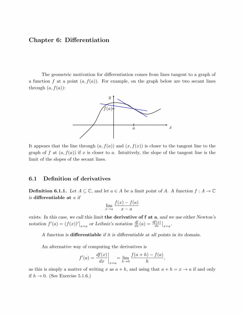
Chapter 6: Differentiation
The geometric motivation for differentiation comes from lines tangent to a graph of
a function f at a point (a, f(a)). For example, on the graph below are two secant lines
through (a, f(a)):
x
y
a
f(a)
It appears that the line through (a, f(a)) and (x, f(x)) is closer to the tangent line to the
graph of f at (a, f(a)) if x is closer to a. Intuitively, the slope of the tangent line is the
limit of the slopes of the secant lines.
6.1 Definition of derivatives
Definition 6.1.1. Let A ⊆ C, and let a ∈ A be a limit point of A. A function f : A→ Cis differentiable at a if
limx→a
f(x)− f(a)
x− a
exists. In this case, we call this limit the derivative of f at a, and we use either Newton’s
notation f ′(a) = (f(x))′∣∣x=a
or Leibniz’s notation dfdx (a) = df(x)
dx
∣∣x=a
.
A function is differentiable if it is differentiable at all points in its domain.
An alternative way of computing the derivatives is
f ′(a) =df(x)
dx
∣∣∣∣x=a
= limh→0
f(a+ h)− f(a)
h,
as this is simply a matter of writing x as a+ h, and using that a+ h = x→ a if and only
if h→ 0. (See Exercise 5.1.6.)
Section 6.1: Definition of derivatives 203
Example 6.1.2. Let f(x) = mx+ l, where m and l are complex numbers. Then for any
a ∈ C, Then
f ′(a) = limx→a
f(x)− f(a)
x− a= limx→a
(mx+ l)− (ma+ l)
x− a= limx→a
m(x− a)
x− a= m.
Alternatively,
f ′(a) = limh→0
f(a+ h)− f(a)
h= limh→0
(m(a+ h) + l)− (ma+ l)
h= limh→0
mh
h= m.
Example 6.1.3. Let f(x) = x2. Then
f ′(a) = limx→a
f(x)− f(a)
x− a
= limx→a
x2 − a2
x− a
= limx→a
(x− a)(x+ a)
x− a= limx→a
(x+ a)
= 2a.
Alternatively,
f ′(a) = limh→0
f(a+ h)− f(a)
h
= limh→0
(a+ h)2 − a2
h
= limh→0
a2 + 2ah+ h2 − a2
h
= limh→0
2ah+ h2
h
= limh→0
(2a+ h)h
h= limh→0
(2a+ h)
= 2a.
From now on, we will mostly use the alternative way of computing derivatives.
Example 6.1.4. Let f(x) = 1/x. Then
f ′(a) = limh→0
f(a+ h)− f(a)
h
= limh→0
1a+h −
1a
h

204 Chapter 6: Differentiation
= limh→0
aa(a+h) −
a+ha(a+h)
h(common denominator in the fractions)
= limh→0
a−a−ha(a+h)
h
= limh→0
−ha(a+ h)h
= limh→0
−1
a(a+ h)
=−1
a2
by the quotient rule for limits.
Example 6.1.5. Let f(x) =√x. The domain of f is R≥0, and for all a > 0,
f ′(a) = limh→0
f(a+ h)− f(a)
h
= limh→0
√a+ h−
√a
h
= limh→0
√a+ h−
√a
h·√a+ h+
√a√
a+ h+√a
= limh→0
(a+ h)− ah(√a+ h+
√a)
(since (x− y)(x+ y) = x2 − y2)
= limh→0
h
h(√a+ h+
√a)
= limh→0
1√a+ h+
√a
=1
2√a
by the linear, radical, composite, and quotient rules for limits. It is left to Exercise 6.1.4
to show that f is not differentiable at 0.
Example 6.1.6. Let f(x) = x3/2. The domain of f is R≥0, and for all a ≥ 0,
f ′(a) = limh→0
f(a+ h)− f(a)
h
= limh→0
(a+ h)3/2 − a3/2
h
= limh→0
(a+ h)3/2 − a3/2
h· (a+ h)3/2 + a3/2
(a+ h)3/2 + a3/2
= limh→0
(a+ h)3 − a3
h((a+ h)3/2 + a3/2)(since (x− y)(x+ y) = x2 − y2)
Section 6.1: Definition of derivatives 205
= limh→0
a3 + 3a2h+ 3ah2 + h3 − a3
h((a+ h)3/2 + a3/2)
= limh→0
(3a2 + 3ah+ h2)h
h((a+ h)3/2 + a3/2)
= limh→0
3a2 + 3ah+ h2
(a+ h)3/2 + a3/2
=
3a2
a3/2+a3/2, if a > 0;
limh→0
h2
h3/2= limh→0
h1/2 = 0, if a = 0;
=3
2a1/2
by the linear, radical, composite, and quotient rules for limits. (Note that this f is differen-
tiable even at 0, whereas the square root function (previous example) is not differentiable
at 0.)
Note that in all these examples, f ′ is a function from some subset of the domain of
f to a subset of C, and we can compute f ′ at a number labeled x rather than a:
f ′(x) =df(x)
dx= limh→0
f(x+ h)− f(x)
h= limz→x
f(z)− f(x)
z − x.
The h-limit is perhaps preferable to the last limit, where it is z that varies and gets closer
and closer to x.
Example 6.1.7. The absolute value function is not differentiable at 0.
Proof. This function is not differentiable whether the domain is C or R. The reason is
that the limit of |h|−|0|h as h goes to 0 does not exist. Namely, if h varies over positive real
numbers, this limit is 1, and if h varies over negative real numbers, the limit is −1, so that
the limit indeed does not exist, and hence the derivative does not exist.
This gives an example of a continuous function that is not differentiable. (Any
continuous function with a jagged graph is not differentiable.)
Exercises for Section 6.1
6.1.1. Prove that f : C→ C given by f(x) = x3 is differentiable everywhere, and compute
the derivative function.
6.1.2. Prove that f : C \ {0} → C given by f(x) = 1/x2 is differentiable everywhere, and
compute the derivative function.
6.1.3. Prove that f : (0,∞)→ R given by f(x) = 1/√x is differentiable everywhere, and
compute the derivative function.

206 Chapter 6: Differentiation
6.1.4. Prove that the square root function is not differentiable at 0.
6.1.5. Prove that the function f : [0,∞) → R given by f(x) = x3/2 is differentiable,
including at 0.
6.1.6. Let f : R→ R be given by
f(x) =
{x2 − 1, if x > 1;x3 − x, if x ≤ 1.
Prove that f is differentiable at 1.
6.1.7. Let f : R→ R be given by
f(x) =
{x2 − 1, if x > 1;x4 − 4x, if x ≤ 1.
Prove that f is continuous but not differentiable at 1.
6.1.8. Let f : R→ R be given by
f(x) =
{x2, if x > 1;x3 − x, if x ≤ 1.
Prove that f is not continuous and not differentiable at 1.
6.1.9. Determine if the following function is differentiable at 1: f(x) =
{x2, if x > 1;2x, if x ≤ 1.
6.1.10. Let f, g : R→ R be f(x) =
{12x
2, if x ≥ 0;− 1
2x2, if x < 0,
and g(x) =
{12x
2 + 3, if x ≥ 0;− 1
2x2, if x < 0.
i) Prove that f is differentiable everywhere and that for all x ∈ R, f ′(x) = |x|.ii) Prove that g is not differentiable at 0.
iii) Prove that g is differentiable at any non-zero real number x with g′(x) = |x|.6.1.11. Let f : (0, 1) → R be the square root function. Verify that f is differentiable,
bounded, even uniformly continuous, and that f ′ is not bounded. (Hint: Example 6.1.5.)
6.2 Basic properties of derivatives
Theorem 6.2.1. If f is differentiable at a, then f is continuous at a.
Proof. By definition of differentiability, a is a limit point of the domain of f and a is in the
domain of f . Furthermore, since limh→0f(a+h)−f(a)
h exists, by the product rule for limits
also limh→0(h f(a+h)−f(a)h ) exists and equals 0 · f ′(a) = 0. In other words, limh→0(f(a +
h) − f(a)) = 0, so that by the sum rule for limits, limh→0 f(a + h) = limh→0(f(a + h) −f(a) + f(a)) = 0 + f(a) = f(a). Thus by Exercise 5.1.6, limx→a f(x) = f(a), so that f is
continuous at a.
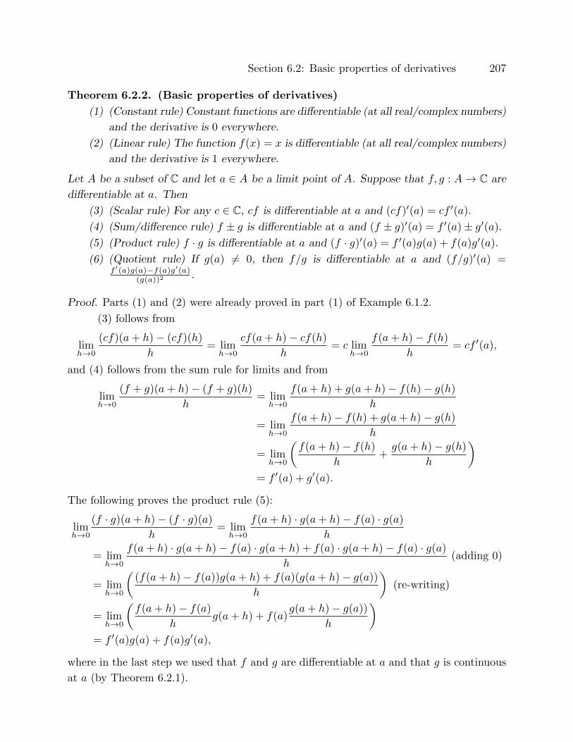
Section 6.2: Basic properties of derivatives 207
Theorem 6.2.2. (Basic properties of derivatives)
(1) (Constant rule) Constant functions are differentiable (at all real/complex numbers)
and the derivative is 0 everywhere.
(2) (Linear rule) The function f(x) = x is differentiable (at all real/complex numbers)
and the derivative is 1 everywhere.
Let A be a subset of C and let a ∈ A be a limit point of A. Suppose that f, g : A→ C are
differentiable at a. Then
(3) (Scalar rule) For any c ∈ C, cf is differentiable at a and (cf)′(a) = cf ′(a).
(4) (Sum/difference rule) f ± g is differentiable at a and (f ± g)′(a) = f ′(a)± g′(a).
(5) (Product rule) f · g is differentiable at a and (f · g)′(a) = f ′(a)g(a) + f(a)g′(a).
(6) (Quotient rule) If g(a) 6= 0, then f/g is differentiable at a and (f/g)′(a) =f ′(a)g(a)−f(a)g′(a)
(g(a))2 .
Proof. Parts (1) and (2) were already proved in part (1) of Example 6.1.2.
(3) follows from
limh→0
(cf)(a+ h)− (cf)(h)
h= limh→0
cf(a+ h)− cf(h)
h= c lim
h→0
f(a+ h)− f(h)
h= cf ′(a),
and (4) follows from the sum rule for limits and from
limh→0
(f + g)(a+ h)− (f + g)(h)
h= limh→0
f(a+ h) + g(a+ h)− f(h)− g(h)
h
= limh→0
f(a+ h)− f(h) + g(a+ h)− g(h)
h
= limh→0
(f(a+ h)− f(h)
h+g(a+ h)− g(h)
h
)= f ′(a) + g′(a).
The following proves the product rule (5):
limh→0
(f · g)(a+ h)− (f · g)(a)
h= limh→0
f(a+ h) · g(a+ h)− f(a) · g(a)
h
= limh→0
f(a+ h) · g(a+ h)− f(a) · g(a+ h) + f(a) · g(a+ h)− f(a) · g(a)
h(adding 0)
= limh→0
((f(a+ h)− f(a))g(a+ h) + f(a)(g(a+ h)− g(a))
h
)(re-writing)
= limh→0
(f(a+ h)− f(a)
hg(a+ h) + f(a)
g(a+ h)− g(a))
h
)= f ′(a)g(a) + f(a)g′(a),
where in the last step we used that f and g are differentiable at a and that g is continuous
at a (by Theorem 6.2.1).

208 Chapter 6: Differentiation
The proof of the quotient rule (6) is similar. It is written out next without a com-
mentary; the reader is encouraged to supply justification for each step:
limh→0
fg (a+ h)− f
g (a)
h= limh→0
f(a+h)g(a+h) −
f(a)g(a)
h
= limh→0
f(a+ h)g(a)− f(a)g(a+ h)
hg(a+ h)g(a)
= limh→0
f(a+ h)g(a)− f(a)g(a) + f(a)g(a)− f(a)g(a+ h)
hg(a+ h)g(a)
= limh→0
f(a+ h) · g(a+ h)− f(a) · g(a+ h) + f(a) · g(a)− f(a) · g(a+ h)
hg(a+ h)g(a)
= limh→0
(f(a+ h) · g(a+ h)− f(a) · g(a+ h)
hg(a+ h)g(a)− f(a) · g(a+ h)− f(a) · g(a)
hg(a+ h)g(a)
)= limh→0
(f(a+ h)− f(a)
h· g(a+ h)
g(a+ h)g(a)− f(a)
g(a+ h)g(a)· g(a+ h)− g(a)
h
)=f ′(a)g(a)− f(a)g′(a)
(g(a))2.
Theorem 6.2.3. (Power rule) If n is a positive integer, then (xn)′ = nxn−1.
Proof #1: Part (1) of Example 6.1.2 with m = 1 and l = 0 proves that (x1)′ = 1, so that
the theorem is true when n = 1. Now suppose that the theorem holds for some positive
integer n. Then
(xn)′ = (xn−1x)′
= (xn−1)′x+ xn−1x′ (by the product rule)
= (n− 1)xn−2x+ xn−1 (by induction assumption)
= (n− 1)xn−1 + xn−1
= nxn−1,
so that the theorem holds also for n, and so by induction also for all positive n.
Proof #2: The second proof uses binomial expansions as in Exercise 1.6.7:
(xn)′ = limh→0
(x+ h)n − xn
h
= limh→0
∑nk=0
(nk
)xkhn−k − xn
h
= limh→0
∑n−1k=0
(nk
)xkhn−k
h
= limh→0
h∑n−1k=0
(nk
)xkhn−k−1
h
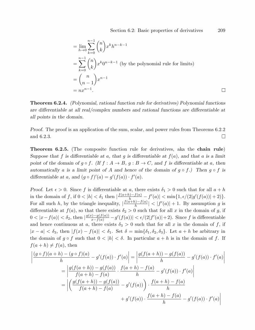
Section 6.2: Basic properties of derivatives 209
= limh→0
n−1∑k=0
(n
k
)xkhn−k−1
=n−1∑k=0
(n
k
)xk0n−k−1 (by the polynomial rule for limits)
=
(n
n− 1
)xn−1
= nxn−1.
Theorem 6.2.4. (Polynomial, rational function rule for derivatives) Polynomial functions
are differentiable at all real/complex numbers and rational functions are differentiable at
all points in the domain.
Proof. The proof is an application of the sum, scalar, and power rules from Theorems 6.2.2
and 6.2.3.
Theorem 6.2.5. (The composite function rule for derivatives, aka the chain rule)
Suppose that f is differentiable at a, that g is differentiable at f(a), and that a is a limit
point of the domain of g ◦ f . (If f : A → B, g : B → C, and f is differentiable at a, then
automatically a is a limit point of A and hence of the domain of g ◦ f .) Then g ◦ f is
differentiable at a, and (g ◦ f)′(a) = g′(f(a)) · f ′(a).
Proof. Let ε > 0. Since f is differentiable at a, there exists δ1 > 0 such that for all a + h
in the domain of f , if 0 < |h| < δ1 then | f(a+h)−f(a)h − f ′(a)| < min{1, ε/(2|g′(f(a))|+ 2)}.
For all such h, by the triangle inequality, | f(a+h)−f(a)h | < |f ′(a)| + 1. By assumption g is
differentiable at f(a), so that there exists δ2 > 0 such that for all x in the domain of g, if
0 < |x−f(a)| < δ2, then | g(x)−g(f(a))x−f(a) −g′(f(a))| < ε/(2|f ′(a)|+2). Since f is differentiable
and hence continuous at a, there exists δ3 > 0 such that for all x in the domain of f , if
|x − a| < δ3, then |f(x) − f(a)| < δ1. Set δ = min{δ1, δ2, δ3}. Let a + h be arbitrary in
the domain of g ◦ f such that 0 < |h| < δ. In particular a + h is in the domain of f . If
f(a+ h) 6= f(a), then∣∣∣∣ (g ◦ f)(a+ h)− (g ◦ f)(a)
h− g′(f(a)) · f ′(a)
∣∣∣∣ =
∣∣∣∣g(f(a+ h))− g(f(a))
h− g′(f(a)) · f ′(a)
∣∣∣∣=
∣∣∣∣g(f(a+ h))− g(f(a))
f(a+ h)− f(a)· f(a+ h)− f(a)
h− g′(f(a)) · f ′(a)
∣∣∣∣=
∣∣∣∣(g(f(a+ h))− g(f(a))
f(a+ h)− f(a)− g′(f(a))
)· f(a+ h)− f(a)
h
+ g′(f(a)) · f(a+ h)− f(a)
h− g′(f(a)) · f ′(a)
∣∣∣∣
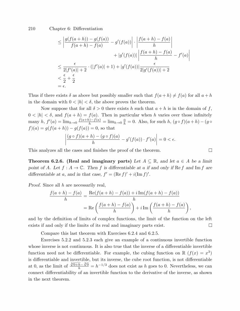
210 Chapter 6: Differentiation
≤∣∣∣∣g(f(a+ h))− g(f(a))
f(a+ h)− f(a)− g′(f(a))
∣∣∣∣ · ∣∣∣∣f(a+ h)− f(a)
h
∣∣∣∣+ |g′(f(a))|
∣∣∣∣f(a+ h)− f(a)
h− f ′(a)
∣∣∣∣≤ ε
2|f ′(a)|+ 2· (|f ′(a)|+ 1) + |g′(f(a))| ε
2|g′(f(a))|+ 2
<ε
2+ε
2= ε.
Thus if there exists δ as above but possibly smaller such that f(a+ h) 6= f(a) for all a+ h
in the domain with 0 < |h| < δ, the above proves the theorem.
Now suppose that for all δ > 0 there exists h such that a+ h is in the domain of f ,
0 < |h| < δ, and f(a + h) = f(a). Then in particular when h varies over those infinitely
many h, f ′(a) = limh→0f(a+h)−f(a)
h = limh→00h = 0. Also, for such h, (g ◦ f)(a+h)− (g ◦
f)(a) = g(f(a+ h))− g(f(a)) = 0, so that∣∣∣∣ (g ◦ f)(a+ h)− (g ◦ f)(a)
h− g′(f(a)) · f ′(a)
∣∣∣∣ = 0 < ε.
This analyzes all the cases and finishes the proof of the theorem.
Theorem 6.2.6. (Real and imaginary parts) Let A ⊆ R, and let a ∈ A be a limit
point of A. Let f : A → C. Then f is differentiable at a if and only if Re f and Im f are
differentiable at a, and in that case, f ′ = (Re f)′ + i(Im f)′.
Proof. Since all h are necessarily real,
f(a+ h)− f(a)
h=
Re(f(a+ h)− f(a)) + i Im(f(a+ h)− f(a))
h
= Re
(f(a+ h)− f(a)
h
)+ i Im
(f(a+ h)− f(a)
h
),
and by the definition of limits of complex functions, the limit of the function on the left
exists if and only if the limits of its real and imaginary parts exist.
Compare this last theorem with Exercises 6.2.4 and 6.2.5.
Exercises 5.2.2 and 5.2.3 each give an example of a continuous invertible function
whose inverse is not continuous. It is also true that the inverse of a differentiable invertible
function need not be differentiable. For example, the cubing function on R (f(x) = x3)
is differentiable and invertible, but its inverse, the cube root function, is not differentiable
at 0, as the limit of3√0+h− 3√0
h = h−1/3 does not exist as h goes to 0. Nevertheless, we can
connect differentiability of an invertible function to the derivative of the inverse, as shown
in the next theorem.
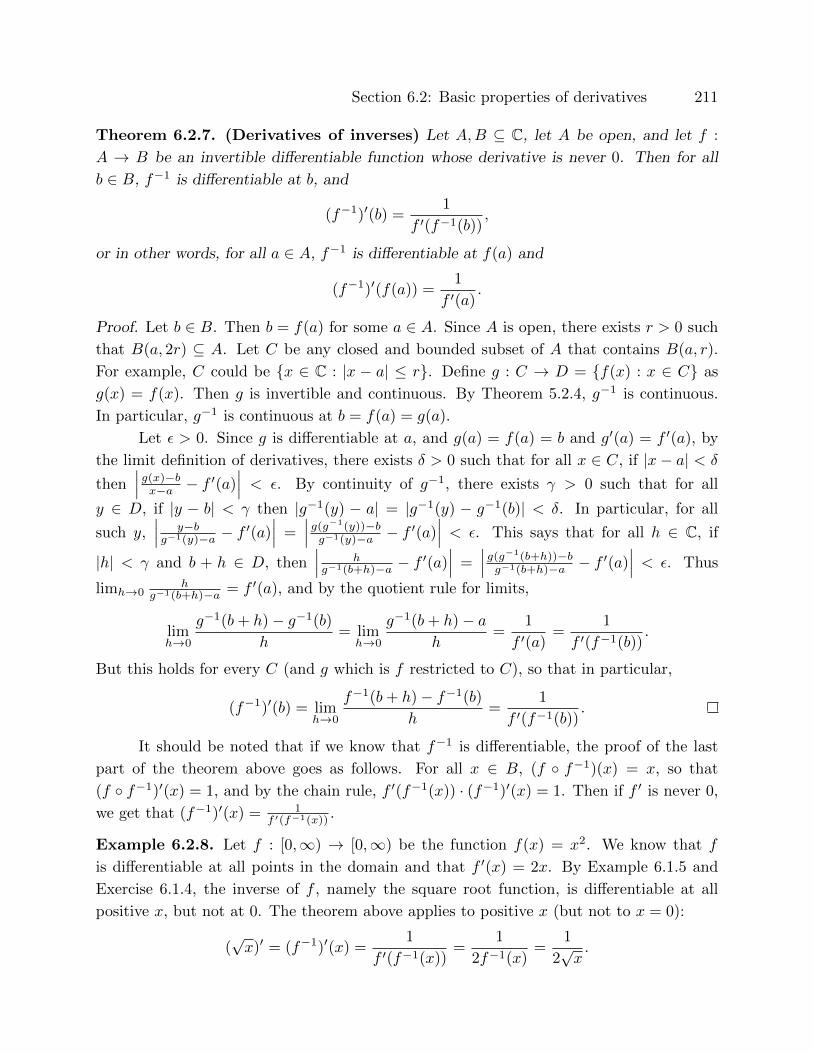
Section 6.2: Basic properties of derivatives 211
Theorem 6.2.7. (Derivatives of inverses) Let A,B ⊆ C, let A be open, and let f :
A → B be an invertible differentiable function whose derivative is never 0. Then for all
b ∈ B, f−1 is differentiable at b, and
(f−1)′(b) =1
f ′(f−1(b)),
or in other words, for all a ∈ A, f−1 is differentiable at f(a) and
(f−1)′(f(a)) =1
f ′(a).
Proof. Let b ∈ B. Then b = f(a) for some a ∈ A. Since A is open, there exists r > 0 such
that B(a, 2r) ⊆ A. Let C be any closed and bounded subset of A that contains B(a, r).
For example, C could be {x ∈ C : |x − a| ≤ r}. Define g : C → D = {f(x) : x ∈ C} as
g(x) = f(x). Then g is invertible and continuous. By Theorem 5.2.4, g−1 is continuous.
In particular, g−1 is continuous at b = f(a) = g(a).
Let ε > 0. Since g is differentiable at a, and g(a) = f(a) = b and g′(a) = f ′(a), by
the limit definition of derivatives, there exists δ > 0 such that for all x ∈ C, if |x− a| < δ
then∣∣∣ g(x)−bx−a − f
′(a)∣∣∣ < ε. By continuity of g−1, there exists γ > 0 such that for all
y ∈ D, if |y − b| < γ then |g−1(y) − a| = |g−1(y) − g−1(b)| < δ. In particular, for all
such y,∣∣∣ y−bg−1(y)−a − f
′(a)∣∣∣ =
∣∣∣ g(g−1(y))−bg−1(y)−a − f
′(a)∣∣∣ < ε. This says that for all h ∈ C, if
|h| < γ and b + h ∈ D, then∣∣∣ hg−1(b+h)−a − f
′(a)∣∣∣ =
∣∣∣ g(g−1(b+h))−bg−1(b+h)−a − f
′(a)∣∣∣ < ε. Thus
limh→0h
g−1(b+h)−a = f ′(a), and by the quotient rule for limits,
limh→0
g−1(b+ h)− g−1(b)
h= limh→0
g−1(b+ h)− ah
=1
f ′(a)=
1
f ′(f−1(b)).
But this holds for every C (and g which is f restricted to C), so that in particular,
(f−1)′(b) = limh→0
f−1(b+ h)− f−1(b)
h=
1
f ′(f−1(b)).
It should be noted that if we know that f−1 is differentiable, the proof of the last
part of the theorem above goes as follows. For all x ∈ B, (f ◦ f−1)(x) = x, so that
(f ◦ f−1)′(x) = 1, and by the chain rule, f ′(f−1(x)) · (f−1)′(x) = 1. Then if f ′ is never 0,
we get that (f−1)′(x) = 1f ′(f−1(x)) .
Example 6.2.8. Let f : [0,∞) → [0,∞) be the function f(x) = x2. We know that f
is differentiable at all points in the domain and that f ′(x) = 2x. By Example 6.1.5 and
Exercise 6.1.4, the inverse of f , namely the square root function, is differentiable at all
positive x, but not at 0. The theorem above applies to positive x (but not to x = 0):
(√x)′ = (f−1)′(x) =
1
f ′(f−1(x))=
1
2f−1(x)=
1
2√x.
212 Chapter 6: Differentiation
Theorem 6.2.9. Let n be a positive integer. Then for all non-zero x in the domain of n√
,
( n√x)′ =
1
nx1/n−1.
Proof. Let A = R+ if n is even and let A = R \ {0} otherwise. Define f : A → A to
be f(x) = xn. We have proved that f is invertible and differentiable. The derivative is
f ′(x) = nxn−1, which is never 0. Thus by the previous theorem, f−1 = n√
is differentiable
with
( n√x)′ =
1
f ′( n√x)
=1
n( n√x)n−1
=1
nx(n−1)/n=
1
nx−(n−1)/n =
1
nx1/n−1.
Theorem 6.2.10. (Generalized power rule) Let r be an arbitrary rational number
and let f : R+ → R+ be given by f(x) = xr. Then for all x, f ′(x) = rxr−1.
Proof. The power rule and quotient rules prove this in case r an integer, and the previous
theorem proves it in case r is one over a positive integer. Now suppose that r = m/n for
some integers m,n with n 6= 0. Since m/n = (−m)/(−n) is also a quotient of two integers,
we may write r = m/n so that m ∈ Z and n is a positive integer. Thus f is the composition
of exponentiation by m and by 1/n. By the chain rule,
f ′(x) = m(x1/n)m−1 · 1
nx1/n−1 =
m
nx(m−1)/n+1/n−1 = rxm/n−1/n+1/n−1 = rxr−1.
This proves the theorem for all rational r.
The theorem also holds for all real r. But to prove it for all real r one first needs to
define exponentiation by non-rational numbers. Such exponentiation was worked through
laboriously in Exercises 5.4.7 and 5.4.8, and if we were to continue that kind of labori-
ous treatment, the proof of the form of the derivative of such exponentiation would also
be laborious. So we postpone the definition of such exponentiation and the proof of its
derivative to Theorem 7.6.4, where with the help of integrals the definition and proofs write
themselves elegantly.
Exercises for Section 6.2
6.2.1. Provide the commentary for the proof of the quotient rule in Theorem 6.2.2.
6.2.2. Let f, g, h be differentiable. Prove that (fgh)′ = f ′gh+fg′h+fgh′. More generally,
prove a product rule formula for the derivative of the product f1 · f2 · · · · · fn.
6.2.3. Prove yet another form of the general power rule for derivatives: If f is
differentiable at a, then for every positive integer n, fn is differentiable at a, and (fn)′(a) =
n(f(a))n−1f ′(a).
6.2.4. Prove that the functions Re, Im : C→ R are not differentiable at any a.
Section 6.3: The Mean value theorem 213
6.2.5. (Compare with Theorem 6.2.6.) Prove that the absolute value function on R is
differentiable at all non-zero a ∈ R. Prove that the absolute value function on C is not
differentiable at any non-zero a ∈ C. (Hint: Let h = (r − 1)a for r near 1.)
6.2.6. The following information is known: c f(c) f ′(c) g(c) g′(c)
0 1 2 6 4
1 −1 0 5 3
2 2 −3 6 −6
3 4 2 3 5
4 0 8 4 7
For each of the following, either provide the derivative or argue that there is not enough
information. In any case, justify every answer.
i) (f − g)′(1) =
ii) (f · g)′(2) =
iii)(fg
)′(3) =
iv) (g ◦ f)′(4) =
6.2.7. A function f is differentiable on (−2, 5) and f(3) = 4, f ′(3) = −1. Let g(x) = 3x.
For each of the statements below determine whether it is true, false, or if there is not
enough information. Explain your reasoning.
i) f is constant.
ii) The slope of the tangent line to the graph of f at 3 is 4.
iii) f is continuous on (−2, 5).
iv) The derivative of (f ◦ g) at 1 is −3.
v) (f + g)′(3) = 2.
6.2.8. Let f(x) = x−1x−2 .
i) Find all a in the domain of f such that the tangent line to the graph of f at a has
slope −1.
ii) Find all a in the domain of f such that the tangent line to the graph of f at a has
slope 2. (Solutions need not be real.)
6.2.9. We assume the following familiar properties of the trigonometric functions: sin is
differentiable on R, sin′ = cos, and when restricted to [−π, π], sin has an inverse. Use
Theorem 6.2.7, the fact that (sin(x))2 + (cos(x))2 = 1, and that on [−π, π] cosine is non-
negative to prove that (sin−1)′(x) = 1√1−x2
.
214 Chapter 6: Differentiation
6.2.10. Make the requisite assumptions about the trigonometric functions to prove the
following:
i) (cos−1)′(x) = −1√1−x2
.
ii) (tan−1)′(x) = 11+x2 .
iii) tan−1(x) + tan−1(
1x
)= π
2 .
6.3 The Mean value theorem
In this section the domains and codomains of all functions are subsets of R.
Theorem 6.3.1. Let f : [a, b] → R, and let c ∈ [a, b] such that f achieves an extreme
value at c (i.e., either for all x ∈ [a, b], f(c) ≤ f(x) or for all x ∈ [a, b], f(c) ≥ f(x)). Then
at least one of the following holds:
(1) c = a;
(2) c = b;
(3) f is not continuous at c;
(4) f is not differentiable at c;
(5) f is differentiable at c and f ′(c) = 0.
Proof. It suffices to prove that if the first four conditions do not hold, then the fifth one
has to hold. So we assume that c 6= a, c 6= b, and that f is differentiable at c.
Suppose that f ′(c) > 0. By the definition of derivative, f ′(c) = limx→cf(x)−f(c)
x−c .
Thus for all x very near c but larger than c, f(x)−f(c)x−c > 0, so that f(x) − f(c) > 0, so
that f does not achieve its maximum at c. Also, for all x very near c but smaller than c,f(x)−f(c)
x−c > 0, so that f(x)− f(c) < 0, so that f does not achieve its minimum at c. This
is a contradiction, so that f ′(c) cannot be positive. Similarly, f ′(c) cannot be negative.
Thus f ′(c) = 0.
Thus to find extreme values of a function, one only has to check if extreme values
occur at the endpoints of the domain, at points where the function is not continuous or
non-differentiable, or where it is differentiable and the derivative is 0. One should be aware
that just because any of the five conditions is satisfied, we need not have an extreme value
of the function. Here are some examples:
(1) The function f : [−1, 1] → R given by f(x) = x3 − x has neither the maximum
nor the minimum at the endpoints.
(2) Let f : [−1, 1]→ R be given by f(x) =
{x, if x > 0;1/2, if x ≤ 0.
Then f is not continuous
at 0 but f does not have a minimum or maximum at 0.
Section 6.3: The Mean value theorem 215
(3) Let f : [−1, 1] → R be given by f(x) =
{x, if x > 0;2x, if x ≤ 0.
Then f is continuous
and not differentiable at 0, yet f does not have a minimum or maximum at 0.
(4) Let f : [−1, 1]→ R be given by f(x) = x3. Then f is differentiable, f ′(0) = 0, but
f does not have a minimum or maximum at 0.
Theorem 6.3.2. (Darboux’s theorem) Let a < b be real numbers, and let f : [a, b]→R be differentiable. Then f ′ has the intermediate value property, i.e., for all k between
f ′(a) and f ′(b) there exists c ∈ [a, b] such that f ′(c) = k.
Proof. If f ′(a) = k, we set c = a, and similarly if f ′(b) = k, we set c = b. So we may
assume that k is strictly between f ′(a) and f ′(b).
The function g : [a, b] → R given by g(x) = f(x) − kx is differentiable, hence
continuous. Note that g′(x) = f ′(x) − k, so that 0 is strictly between g′(a) and g′(b).
If g′(a) > 0, let c ∈ [a, b] such that g achieves a maximum at c, and if g′(a) < 0, let
c ∈ [a, b] such that g achieves a minimum at c. Such c exists by the Extreme value theorem
(Theorem 5.2.2). Note that g′(a) < 0 if and only if f ′(a) < k, which holds if and only
if f ′(b) > k, which in turn holds if and only if g′(b) > 0. Similarly g′(a) > 0 if and
only if g′(b) < 0. Thus for both choices of c, c cannot be a or b, so that c ∈ (a, b). By
Theorem 6.3.1, g′(c) = 0. Hence f ′(c) = k.
Theorem 6.3.3. (Rolle’s theorem) Let a, b ∈ R with a < b, and let f : [a, b]→ R be a
continuous function such that f is differentiable on (a, b). If f(a) = f(b), then there exists
c ∈ (a, b) such that f ′(c) = 0.
Proof. By the Extreme value theorem (Theorem 5.2.2) there exist l, u ∈ [a, b] such that
f achieves its minimum at l and its maximum at u. If f(l) = f(u), then the minimum
value of f is the same as the maximum value of f , so that f is a constant function, and so
f ′(c) = 0 for all c ∈ (a, b).
Thus we may assume that f(l) 6= f(u). It may be that f achieves its minimum at
the two endpoints, in which case u must be strictly between a and b. Similarly, it may be
that f achieves its maximum at the two endpoints, in which case l must be strictly between
a and b. In all cases of f(l) 6= f(u), either l or u is not the endpoint.
Say that l is not the endpoint. Then a < l < b. For all x ∈ [a, b], f(x) ≥ f(l),
so that in particular for all x ∈ (a, l), f(x)−f(l)x−l ≤ 0 and for all x ∈ (l, b), f(x)−f(l)
x−l ≥ 0.
Since f ′(l) = limx→lf(x)−f(l)
x−l exists, it must be both non-negative and non-positive, so
necessarily it has to be 0.
If instead u is not the endpoint, then a < u < b and for all x ∈ [a, b], f(x) ≤ f(u).
Thus in particular for all x ∈ (a, u), f(x)−f(u)x−u ≥ 0 and for all x ∈ (u, b), f(x)−f(u)
x−u ≤ 0.
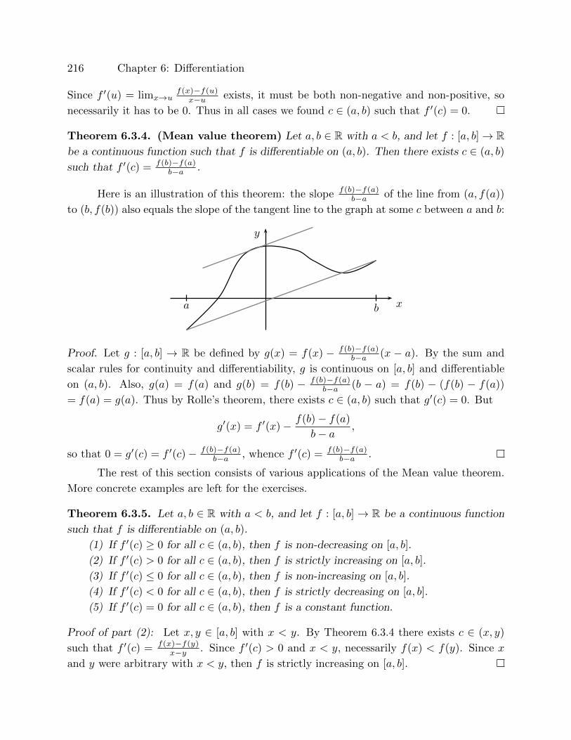
216 Chapter 6: Differentiation
Since f ′(u) = limx→uf(x)−f(u)
x−u exists, it must be both non-negative and non-positive, so
necessarily it has to be 0. Thus in all cases we found c ∈ (a, b) such that f ′(c) = 0.
Theorem 6.3.4. (Mean value theorem) Let a, b ∈ R with a < b, and let f : [a, b]→ Rbe a continuous function such that f is differentiable on (a, b). Then there exists c ∈ (a, b)
such that f ′(c) = f(b)−f(a)b−a .
Here is an illustration of this theorem: the slope f(b)−f(a)b−a of the line from (a, f(a))
to (b, f(b)) also equals the slope of the tangent line to the graph at some c between a and b:
x
y
a b
Proof. Let g : [a, b] → R be defined by g(x) = f(x) − f(b)−f(a)b−a (x − a). By the sum and
scalar rules for continuity and differentiability, g is continuous on [a, b] and differentiable
on (a, b). Also, g(a) = f(a) and g(b) = f(b) − f(b)−f(a)b−a (b − a) = f(b) − (f(b) − f(a))
= f(a) = g(a). Thus by Rolle’s theorem, there exists c ∈ (a, b) such that g′(c) = 0. But
g′(x) = f ′(x)− f(b)− f(a)
b− a,
so that 0 = g′(c) = f ′(c)− f(b)−f(a)b−a , whence f ′(c) = f(b)−f(a)
b−a .
The rest of this section consists of various applications of the Mean value theorem.
More concrete examples are left for the exercises.
Theorem 6.3.5. Let a, b ∈ R with a < b, and let f : [a, b] → R be a continuous function
such that f is differentiable on (a, b).
(1) If f ′(c) ≥ 0 for all c ∈ (a, b), then f is non-decreasing on [a, b].
(2) If f ′(c) > 0 for all c ∈ (a, b), then f is strictly increasing on [a, b].
(3) If f ′(c) ≤ 0 for all c ∈ (a, b), then f is non-increasing on [a, b].
(4) If f ′(c) < 0 for all c ∈ (a, b), then f is strictly decreasing on [a, b].
(5) If f ′(c) = 0 for all c ∈ (a, b), then f is a constant function.
Proof of part (2): Let x, y ∈ [a, b] with x < y. By Theorem 6.3.4 there exists c ∈ (x, y)
such that f ′(c) = f(x)−f(y)x−y . Since f ′(c) > 0 and x < y, necessarily f(x) < f(y). Since x
and y were arbitrary with x < y, then f is strictly increasing on [a, b].
Section 6.3: The Mean value theorem 217
Example 6.3.6. Assuming that sin′(x) ≤ 1 for all x ∈ R (this is proved in Section 9.9),
we have that sin(x) ≤ x for all x ≥ 0.
Proof. Let f(x) = x − sin(x). Then f is differentiable on R, and f ′(x) = 1 − sin′(x) ≥ 0.
By the previous theorem, f is non-decreasing, so that for all x ≥ 0, x − sin(x) = f(x) ≥f(0) = 0, whence x ≥ sin(x).
Theorem 6.3.7. (Convexity of graphs)Let f be a function that is continuous on [a, b]
and twice-differentiable on (a, b).
(1) If f ′′ ≥ 0 on (a, b), then the graph of the function lies below the line connecting
(a, f(a)) and (b, f(b)).
(2) If f ′′ ≤ 0 on (a, b), then the graph of the function lies above the line connecting
(a, f(a)) and (b, f(b)).
Proof. The equation of the line is y = f(b)−f(a)b−a (x− a) + f(a).
(i) Let x ∈ (a, b). We need to prove that f(x) ≤ f(b)−f(a)b−a (x − a) + f(a). By
Theorem 6.3.4 there exists c ∈ (a, x) such that f ′(c) = f(x)−f(a)x−a , and there exists d ∈ (a, x)
such that f ′(d) = f(b)−f(x)b−x . Since f ′′ > 0 and c < x < d, necessarily f(x)−f(a)
x−a ≤ f(b)−f(x)b−x .
By cross-multiplying by positive (x− a)(b− x) we get that
(f(x)− f(a))(b− x) ≤ (f(b)− f(x))(x− a),
or in other words, that f(x)(b − a) ≤ f(a)(b − x) + f(b)(x − a) = f(a)(b − a) + (f(b) −f(a))(x− a), and by dividing by positive b− a yields the desired inequality.
The proof of (ii) is similar.
Theorem 6.3.8. (Cauchy’s mean value theorem) Let a < b be real numbers and let
f, g : [a, b]→ R be continuous functions that are differentiable on (a, b). Then there exists
c ∈ (a, b) such that
f ′(c)(g(b)− g(a)) = g′(c)(f(b)− f(a)).
In particular, if g′(c) 6= 0 and g(b) 6= g(a), this says that f ′(c)g′(c) = f(b)−f(a)
g(b)−g(a) .
Proof. Define h : [a, b]→ R by h(x) = f(x)(g(b)−g(a))−g(x)(f(b)−f(a)). Then h is con-
tinuous on [a, b] and differentiable on (a, b). Note that h(a) = f(a)(g(b)−g(a))−g(a)(f(b)−f(a)) = f(a)g(b) − g(a)f(b) = h(b). Then by the Mean value theorem (Theorem 6.3.4)
there exists c ∈ (a, b) such that h′(c) = 0, i.e., 0 = f ′(c)(g(b)− g(a))− g′(c)(f(b)− f(a)).

218 Chapter 6: Differentiation
Theorem 6.3.9. (Cauchy’s mean value theorem, II) Let a < b be real numbers and
let f, g : [a, b] → R be continuous functions that are differentiable on (a, b) and such that
g′ is non-zero on (a, b). Then g(b) 6= g(a), and there exists c ∈ (a, b) such that
f ′(c)
g′(c)=f(b)− f(a)
g(b)− g(a).
Proof. By the Mean value theorem (Theorem 6.3.4) there exists c ∈ (a, b) such that
g′(c) = g(b)−g(a)b−a . By assumption, g′(c) 6= 0, so that g(b) 6= g(a). The rest follows by
Cauchy’s mean value theorem (Theorem 6.3.8).
Exercises for Section 6.3
6.3.1. Let f : R→ R be a polynomial function of degree n.
i) If f has m distinct roots, prove that f ′ has at least m− 1 distinct roots.
ii) Suppose that f has n distinct roots. Prove that f ′ has exactly n− 1 distinct roots.
(You may need Theorem 2.4.13.)
iii) Give an example of f with n = 2, where f has no roots but f ′ has 1 root. Why
does this not contradict the first part?
6.3.2. Let f : [0, 1]→ C be given by f(x) = x3 + ix2. Prove that there exists no c between
0 and 1 such that f ′(c) = f(1)−f(0)1−0 . Does this contradict the Mean value theorem?
6.3.3. Let f : [a, b] → C be continuous on [a, b] and differentiable on (a, b). Prove that
there exist c, d ∈ (a, b) such that Re(f ′(c)) = Re( f(b)−f(a)
b−a)
and Im(f ′(d)) = Im( f(b)−f(a)
b−a).
Give an example showing that c may not equal to d. Does this contradict the Mean value
theorem?
6.3.4. Prove the remaining parts of Theorem 6.3.5.
6.3.5. This water-filled urn is getting drained at a constant rate through a hole at the
bottom. Plot the function of depth (d) as a function of time.
d

Section 6.4: L’Hopital’s rule 219
6.3.6. Let A be an open interval in R, and let f : A→ R be differentiable with a bounded
derivative function. Prove that f is uniformly continuous.
6.4 L’Hopital’s rule
The domains and codomains of all functions in this section are subsets of R.
Theorem 6.4.1. (L’Hopital’s rule, easiest version) Let A ⊂ C, let a ∈ A be a limit
point of A, and f, g : A→ C such that
(1) f(a) = g(a) = 0.
(2) f and g are differentiable at a.
(3) g′(a) 6= 0.
Then limx→a
f(x)
g(x)=f ′(a)
g′(a).
Proof. limx→a
f(x)
g(x)= limx→a
f(x)− f(a)
g(x)− g(a)(since f(a) = g(a) = 0)
= limx→a
f(x)−f(a)x−a
g(x)−g(a)x−a
=f ′(a)
g′(a)(by the quotient rule for limits since g′(a) 6= 0).
The rest of the versions of L’Hopital’s rule in this section only work for real-valued
functions on domains that are subsets of R.
Theorem 6.4.2. (L’Hopital’s rule) Let a ∈ R and let f, g be real-valued functions
defined on an interval containing a such that
(1) f(a) = g(a) = 0.
(2) f and g are differentiable near a but not necessarily at a.
(3) g′ is non-zero near a. (This is a condition for x near a but not equal to a.)
(4) limx→a
f ′(x)
g′(x)= L.
Then limx→a
f(x)
g(x)= L.
Proof. Let ε > 0. Since limx→a
f ′(x)g′(x) = L, there exists δ > 0 such that for all x in the domain, if
0 < |x−a| < δ then | f′(x)g′(x)−L| < ε. Let x be one such number. By Theorem 6.3.9 there exists
a number c strictly between a and x such that f ′(c)g′(c) = f(x)−f(a)
g(x)−g(a) . Since f(a) = g(a) = 0,
220 Chapter 6: Differentiation
this says that f ′(c)g′(c) = f(x)
g(x) . Since 0 < |x− a| < δ and c is between a and x, it follows that
0 < |c− a| < δ. Hence ∣∣∣∣f(x)
g(x)− L
∣∣∣∣ =
∣∣∣∣f ′(c)g′(c)− L
∣∣∣∣ < ε.
With our definition of derivatives, this last version includes the one-sided cases where
the domains for f and g are of the form [a, b), or of the form (b, a].
I should note that many books omit hypothesis (3). A counterexample if we omit
that hypothesis is given in Exercise 9.11.5.
The versions of L’Hopital’s rule so far deal with limits of the form “zero over zero”.
There are similarly three versions for the form “infinity over infinity”. I write and prove
only the right-sided version:
Theorem 6.4.3. (L’Hopital’s rule) Let a < b be real numbers. Let f, g : (a, b)→ R be
differentiable with the following properties:
(1) limx→b−
f(x) = limx→b−
g(x) =∞.
(2) For all x ∈ (a, b), g′(x) 6= 0.
(3) limx→b−
f ′(x)
g′(x)= L.
Then limx→b−
f(x)
g(x)= L.
Proof. Let ε > 0. By assumption there exists δ1 > 0 such that for all x ∈ (a, b), if
0 < b− x < δ1, then∣∣∣ f ′(x)g′(x) − L
∣∣∣ < ε/4. By possibly replacing δ1 by min{δ1, (b− a)/2} we
may assume that b− δ1 > a.
Set a0 = b − δ1. Fix x such that 0 < b − x < δ1. Then x ∈ (a0, b) ⊆ (a, b). By
Theorem 6.3.9 there exists c ∈ (a0, x) such that f ′(c)g′(c) = f(x)−f(a0)
g(x)−g(a0) , and so∣∣∣∣f(x)− f(a0)
g(x)− g(a0)− L
∣∣∣∣ =
∣∣∣∣f ′(c)g′(c)− L
∣∣∣∣ < ε/4.
Since limx→b−
f(x) = limx→b−
g(x) = ∞, there exists δ2 > 0 such that for all x with
0 < b− x < δ2, f(x) and g(x) are non-zero, and so we can define h : (b− δ2, b)→ R as
h(x) =1− f(a0)
f(x)
1− g(a0)g(x)
.
By Theorem 4.4.7, limx→b− h(x) = 1. Thus there exists δ3 > 0 such that for all x, if
0 < b − x < δ3, then |h(x)− 1| < min{ε/4(|L| + 1), 12}. The ( 1
2 )-restriction in particular
means that h(x) > 12 . Set δ = min{δ1, δ2, δ3}. Then for all x with 0 < b− x < δ,∣∣∣∣f(x)
g(x)− L
∣∣∣∣ =
∣∣∣∣f(x)
g(x)h(x)− Lh(x)
∣∣∣∣ 1
|h(x)|
Section 6.4: L’Hopital’s rule 221
=
∣∣∣∣f(x)− f(a0)
g(x)− g(a0)− Lh(x)
∣∣∣∣ 1
|h(x)|
≤ 2
∣∣∣∣f(x)− f(a0)
g(x)− g(a0)− Lh(x)
∣∣∣∣ (since |h(x)| > 1/2)
≤ 2
(∣∣∣∣f(x)− f(a0)
g(x)− g(a0)− L
∣∣∣∣+ |L− Lh(x)|)
(by the triangle inequality)
= 2
(∣∣∣∣f ′(c)g′(c)− L
∣∣∣∣+ |L| |1− h(x)|)
< 2( ε
4+ε
4
)= ε.
Example 6.4.4. Compute limx→1
x2−1x3−1 .
Proof #1: By Example 1.5.4, x2−1x3−1 = (x−1)(x+1)
(x−1)(x2+x+1) , so that by Exercise 4.3.10 and Theo-
rem 4.3.6, limx→1
x2−1x3−1 = lim
x→1
x+1x2+x+1 = 1+1
12+1+1 = 23 .
Proof #2: By Theorem 4.3.5, limx→1
(x2 − 1) = 0 = limx→1
(x3 − 1), limx→1
(x2 − 1)′ = limx→1
2x = 2,
and limx→1
(x3 − 1)′ = limx→1
3x2 = 3. Thus by L’Hopital’s rule (Theorem 6.4.2), limx→1
x2−1x3−1
equals 23 .
More forms of L’Hopital’s rule are in the exercises below, as well as in Section 9.11
after the exponential and trigonometric functions have been covered.
Exercises for Section 6.4
6.4.1. Compute and justify limx→−8
x2−643√x+2
.
6.4.2. What is wrong with the following: Since limx→22x2 = 2, by L’Hopital’s rule we
have that limx→2x2+32x−3 = 2.
6.4.3. Let n be a positive integer and a ∈ C. Use L’Hopital’s rule to prove that
limx→axn−anx−a = nan−1. (We have proved the case of a = 1 previously, say how.)
6.4.4. Explicitly state the assumptions about properties of trigonometric functions that
are necessary to prove limx→0
sin(x)x = 1 and lim
x→0
1−cos(x)x = 0.
222 Chapter 6: Differentiation
6.4.5. (Here the goal is to prove another version of L’Hopital’s rule) Let f, g : (a,∞)→ Rbe differentiable. Suppose that lim
x→∞f(x) = lim
x→∞g(x) =∞, that g′(x) is non-zero for all x,
and that limx→∞
f ′(x)g′(x) = L.
i) Let ε > 0. Prove that there exists N > a such that for all x > N , | f′(x)g′(x) − L| < ε.
ii) Prove that there exists N ′ > N such that for all x ≥ N ′, f(x), g(x) > 0.
iii) Prove that there exists N ′′ > N ′ such that for all x ≥ N ′′, f(x) > f(N ′) and
g(x) > g(N ′).
iv) Prove that for all x > N ′′ there exists c ∈ (N ′, x) such that f ′(c)g′(c) = f(x)
g(x)1−f(N ′)/f(x)1−g(N ′)/g(x) .
v) Prove that limx→∞
f(x)g(x) = L.
6.4.6. (Yet another version of L’Hopital’s rule) Let f, g : (a,∞) → R be differentiable.
Suppose that limx→∞
f(x) = limx→∞
g(x) = 0, that g′(x) is non-zero for all x, and that limx→∞
f ′(x)g′(x) = L. Prove that lim
x→∞f(x)g(x) = L.
6.5 Higher-order derivatives, Taylor polynomials
Let f be a function from a subset of C to C.
If f is continuous at a, then near a, f is approximately the constant function f(a)
because limx→a f(x) = f(a). Among all constant functions, the function y = f(a) approx-
imates f at a best.
If f is differentiable near a and the derivative is continuous at a, then for all x near a
but not equal to a, f(x) = f(x)−f(a)+f(a) = f(x)−f(a)x−a (x−a)+f(a) ∼= f ′(a)(x−a)+f(a),
so that for x near a (and possibly equal to a), f is approximately the linear function
f ′(a)(x− a) + f(a), i.e., f is approximated by its tangent line.
This game keeps going, but for this we need higher order derivatives:
Definition 6.5.1. Let f be differentiable. If f ′ is differentiable, we write the derivative
of f ′ as f ′′, or as f (2). If f (n−1) is differentiable, we denote its derivative as f (n). We say
that f has the nth derivative, or that it has derivatives up to order n.
Using this notation we also write f (1) = f ′ and f (0) = f .
If f(x) = xm, then for all n ≤ m, f (n)(x) = m(m− 1)(m− 2) · · · (m− n+ 1)xm−n.
Section 6.5: Higher-order derivatives, Taylor polynomials 223
Definition 6.5.2. Let f be a function with derivatives of orders 1, 2, . . . , n existing at a
point a in the domain. The Taylor polynomial of f (centered) at a of order n is
Tn,f,a(x) = f(a) + f ′(a)(x− a) +f ′′(a)
2!(x− a)2 + · · ·+ f (n)(a)
n!(x− a)n
=n∑k=0
f (k)(a)
k!(x− a)k.
Example 6.5.3. If f(x) = x4 − 3x3 + 4x2 + 7x− 10, then with a = 0,
T0,f,0(x) = −10,
T1,f,0(x) = −10 + 7x,
T2,f,0(x) = −10 + 7x+ 4x2,
T3,f,0(x) = −10 + 7x+ 4x2 − 3x3,
Tn,f,0(x) = −10 + 7x+ 4x2 − 3x3 + x4 for all n ≥ 4,
and for a = 1,
T0,f,1(x) = −1,
T1,f,1(x) = −1 + 10(x− 1),
T2,f,1(x) = −1 + 10(x− 1) + (x− 1)2,
T3,f,1(x) = −1 + 10(x− 1) + (x− 1)2 + (x− 1)3,
Tn,f,1(x) = −1 + 10(x− 1) + (x− 1)2 + (x− 1)3 + (x− 1)4 for all n ≥ 4.
Note that for all n ≥ 4, Tn,f,0(x) = Tn,f,1(x) = f(x).
The following is a generalization of this observation:
Theorem 6.5.4. If f is a polynomial of degree at most d, then for any a ∈ C and any
integer n ≥ d, the nth-order Taylor polynomial of f centered at a equals f .
Proof. Write f(x) = c0+c1x+· · ·+cdxd for some c0, c1, . . . , cd ∈ C. By elementary algebra,
it is possible to rewrite f in the form f(x) = e0 + e1(x− a) + e2(x− a)2 + · · ·+ ed(x− a)d
for some e0, e1, . . . , ed ∈ C. Now observe that
f(a) = e0,
f ′(a) = e1,
f ′′(a) = 2e2,
f ′′′(a) = 6e3 = 3!e3,
f (4)(a) = 24e4 = 4!e4,
...
224 Chapter 6: Differentiation
f (k)(a) = k!ek if k ≤ d,f (k)(a) = 0 if k > d.
But then for n ≥ d,
Tn,f,a(x) =n∑k=0
f (k)(a)
k!(x− a)k =
d∑k=0
k!ekk!
(x− a)k =d∑k=0
ek(x− a)k = f(x).
Theorem 6.5.5. (Taylor’s remainder theorem over R) Let I be an interval in R,
and let (a − r, a + r) = B(a, r) ⊆ I. Suppose that f : I → R has derivatives of orders
1, 2, . . . , n + 1 on B(a, r). Then for all x ∈ B(a, r) there exist c, d between a and x such
that
f(x) = Tn,f,a(x) +f (n+1)(c)
n!(x− a)(x− c)n,
f(x) = Tn,f,a(x) +f (n+1)(d)
(n+ 1)!(x− a)n+1.
Proof. Let g : B(a, r)→ R be defined by
g(t) =n∑k=0
f (k)(t)
k!(x− t)k.
Then g is differentiable on B(a, r), and
g′(t) =n∑k=0
f (k+1)(t)
k!(x− t)k −
n∑k=0
kf (k)(t)
k!(x− t)k−1
=f (n+1)(t)
n!(x− t)n +
n−1∑k=0
f (k+1)(t)
k!(x− t)k −
n∑k=1
f (k)(t)
(k − 1)!(x− t)k−1
=f (n+1)(t)
n!(x− t)n.
Note that g(x) = f(x), g(a) = Tn,f,a(x). By the Mean value theorem (Theorem 6.3.4),
there exists c strictly between a and x such that g′(c)(x−a) = g(x)−g(a). In other words,f(n+1)(c)
n! (x− c)n(x− a) = f(x)− Tn,f,a(x), which proves the first formulation.
By Cauchy’s mean value theorem (Theorem 6.3.8) applied to functions g(t) and
h(t) = (x−t)n+1, there exists d between x and a such that h′(d)(g(x)−g(a)) = g′(d)(h(x)−h(a)). In other words,
−(n+ 1)(x− d)n(f(x)− Tn,f,a(x)) =f (n+1)(d)
n!(x− d)n(0− (x− a)n+1).
Since d is not equal to x, we get that −(n+ 1)(f(x)− Tn,f,a(x)) = f(n+1)(d)n! (−(x− a)n+1),
which proves the second formulation.

Section 6.5: Higher-order derivatives, Taylor polynomials 225
Theorem 6.5.6. (Taylor’s remainder theorem over C) Let A be a subset of C or
of R, let a ∈ A, and let r ∈ R+ such that B(a, r) ⊆ A. Let f : A → C have higher order
derivatives of orders 1, 2, . . . , n on B(a, r) with n ≥ 1. Then for every ε > 0 there exists
δ > 0 such that if x ∈ B(a, δ), then
|f(x)− Tn,f,a(x)| < ε.
Proof. Let ε > 0. Let M = 1 + max{|f(a)|, |f ′(a)|, . . . , |f (n)(a)|}. Since f is differentiable
at a, it is continuous at a, so there exists δ1 > 0 such that for all x ∈ B(a, r), if |x−a| < δ1,
then |f(x)−f(a)| < ε/(n+1). Set δ = min{r, δ1, ε/(M(n+1)), 2
√ε
(M(n+1)) , . . .n
√ε
(M(n+1))}.Let x satisfy |x− a| < δ. Then x is in the domain of f and Tn,f,a, and
|f(x)− Tn,f,a(x)| =∣∣∣∣f(x)− f(a)− f ′(a)(x− a)− f ′′(a)
2!(x− a)2 − · · · − f (n)(a)
n!(x− a)n
∣∣∣∣≤ |f(x)− f(a)|+ |f ′(a)| |x− a|+
∣∣∣∣f ′′(a)
2!
∣∣∣∣ |x− a|2 + · · ·+∣∣∣∣f (n)(a)
n!
∣∣∣∣ |x− a|n<
ε
n+ 1+M
ε
M(n+ 1)+M
ε
M(n+ 1)+ · · ·+M
ε
M(n+ 1)
= ε.
More on Taylor polynomials and Taylor series is in the exercises in this section, in
Exercise 7.4.9, and in Section 9.3.
Exercises for Section 6.5
6.5.1. (The second derivative test) Let f : [a, b] → R be differentiable on (a, b) and
suppose that f ′ is differentiable on (a, b) as well. Suppose that f ′(c) = 0 for some c ∈ (a, b).
i) Suppose that f ′′(c) > 0. Prove that f achieves a minimum at c.
ii) Suppose that f ′′(c) < 0. Prove that f achieves a maximum at c.
iii) Suppose that f ′′(c) = 0. By examples show that any of the following are possible:
a) f achieves a minimum at c, b) f achieves a maximum at c, c) f does not have
an extreme point at c.
6.5.2. Prove that if f is a polynomial function, then for every a ∈ R, Tn,f,a = f for all n
greater than or equal to the degree of f .
6.5.3. (Generalized product rule.) Suppose that f and g have derivatives of orders 1, . . . , n
at a. Prove that
(f · g)(n)(a) =
n∑k=0
(n
k
)f (k)(a)g(n−k)(a).
226 Chapter 6: Differentiation
6.5.4. (Generalized quotient rule.) Prove the following generalization of the product rule:
Suppose that f and g have derivatives of orders 1, . . . , n at a and that g(a) 6= 0. Find and
prove a formula for the nth derivative of the function f/g.
6.5.5. Compute the Taylor polynomial of f(x) =√
1 + x of degree 5 centered at a = 0.
Justify your work.
6.5.6. Compute the Taylor polynomial of f(x) =√
1− x of degree 10 centered at a = 0.
Justify your work.
6.5.7. Let n ∈ N0 be given. Justify all work below.
i) Compute the Taylor polynomial of f(x) = 11−x of degree n centered at a = 0.
ii) Compute Tn,f,0(0.5). (Hint: Use Example 1.5.4.)
iii) Compute Tn,f,0(0.5)− f(0.5).
iv) Compute n such that |Tn,f,0(0.5)− f(0.5)| < 0.001.
v) Try to use Theorem 6.5.5 to determine n such that |Tn,f,0(0.5) − f(0.5)| < 0.001.
Note that this usage is not fruitful.
vi) Use Theorem 6.5.5 to determine n such that |Tn,f,0(0.4)− f(0.4)| < 0.001.
6.5.8. Explicitly assume the necessary properties of trigonometric functions to compute
the Taylor polynomials of degree n of sin and cos centered at a = 0.
i) Estimate the error term with Theorem 6.5.5.
ii) In fact, calculators and computers use Taylor polynomials to compute values of
trigonometric and also exponential functions. Compute sin(1) and sin(100) to
within 0.01 of true value. What degree Taylor polynomial suffices for each? Use
Theorem 6.5.5.
6.5.9. Let f : C→ R be the absolute value function.
i) Prove that f has derivatives of all orders at all non-zero numbers.
ii) Compute T2,f,i.
6.5.10. Let f : R→ R be given by f(x) = |x|3.
i) Prove that f is differentiable, and compute f ′.
ii) Prove that f ′ is differentiable, and compute f ′′.
iii) Prove that f ′′ is not differentiable.
6.5.11. Find a differentiable function f : R→ R such that f ′ is not differentiable.
6.5.12. Find a function f : R → R that has derivatives of orders 1, 2, 3, 4, but such that
f (4) is not differentiable.
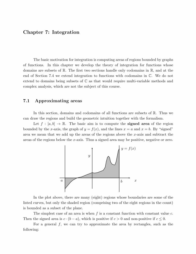
Chapter 7: Integration
The basic motivation for integration is computing areas of regions bounded by graphs
of functions. In this chapter we develop the theory of integration for functions whose
domains are subsets of R. The first two sections handle only codomains in R, and at the
end of Section 7.4 we extend integration to functions with codomains in C. We do not
extend to domains being subsets of C as that would require multi-variable methods and
complex analysis, which are not the subject of this course.
7.1 Approximating areas
In this section, domains and codomains of all functions are subsets of R. Thus we
can draw the regions and build the geometric intuition together with the formalism.
Let f : [a, b] → R. The basic aim is to compute the signed area of the region
bounded by the x-axis, the graph of y = f(x), and the lines x = a and x = b. By “signed”
area we mean that we add up the areas of the regions above the x-axis and subtract the
areas of the regions below the x-axis. Thus a signed area may be positive, negative or zero.
ba x
y
y = f(x)
In the plot above, there are many (eight) regions whose boundaries are some of the
listed curves, but only the shaded region (comprising two of the eight regions in the count)
is bounded as a subset of the plane.
The simplest case of an area is when f is a constant function with constant value c.
Then the signed area is c · (b− a), which is positive if c > 0 and non-positive if c ≤ 0.
For a general f , we can try to approximate the area by rectangles, such as the
following:

228 Chapter 7: Integration
ba x
y
y = f(x)
It may be hard to decide how close the approximation is to the true value. But we
can approximate the region more systematically, by having heights of the rectangles be
either the least possible height or the largest possible height, as below:
ba ba
Then clearly the true area is larger than the sum of the areas of the darker rectangles
on the left and smaller than the sum of the areas of the darker rectangles on the right.
We establish some notation for all this.
Definition 7.1.1. A function f : A → C is bounded if the range {f(x) : x ∈ A} of f is
a bounded subset of C.
Remark 7.1.2. If f is a bounded function with codomain R, then by the Least upper
bound property/theorem (Theorem 3.8.5), for any subset B of the domain, sup{f(x) : x ∈B} and inf{f(x) : x ∈ B} are real numbers.
Definition 7.1.3. A partition of [a, b] is a finite subset of [a, b] that contains a and b.
We typically write a partition in the form P = {x0, x1, . . . , xn}, where x0 = a < x1 < x2 <
· · · < xn−1 < xn = b. (For example, in the figures above, n = 10.)
The sub-intervals of the partition P are [x0, x1], [x1, x2], . . ., [xn−1, xn]. (When
n ≥ 5, the sub-interval [x1, x5] of the interval [a, b] is not a sub-interval of the partition!)
Section 7.1: Approximating areas 229
Definition 7.1.4. Let P = {x0, x1, . . . , xn} be a partition of [a, b] and let f : [a, b] → Rbe a bounded function. The lower sum of f with respect to P is
L(f, P ) =n∑k=1
inf{f(x) : x ∈ [xk−1, xk]}(xk − xk−1).
The upper sum of f with respect to P is
U(f, P ) =
n∑k=1
sup{f(x) : x ∈ [xk−1, xk]}(xk − xk−1).
By Remark 7.1.2, L(f, P ) and U(f, P ) are real numbers.
Clearly if f is a constant function f(x) = c for all x, then all lower and all upper
sums are c(b − a), so that every lower and every upper sum equals c(b − a). If instead f
is a non-constant function, then for every partition P there exists at least one sub-interval
of P on which the supremum of the values of f is strictly bigger than the infimum of such
values, so that L(f, P ) < U(f, P ).
By the geometric set-up for all partitions P of [a, b],
L(f, P ) ≤ the signed area ≤ U(f, P ). (7.1.5)
In particular, if U(f, P )−L(f, P ) < ε, then either U(f, P ) or L(f, P ) serves as an approx-
imation of the true signed area within ε of its true value. For most functions a numerical
approximation is the best we can hope for.
Theorem 7.1.6. If f(x) = c for all x ∈ [a, b], then for any partition P of [a, b], L(f, P ) =
U(f, P ) = c(b− a).
Proof. Let P = {x0, . . . , xn} be a partition of [a, b]. For every k ∈ 1, . . . , n,
inf{f(x) : x ∈ [xk−1, xk]} = sup{f(x) : x ∈ [xk−1, xk]} = c,
so that
L(f, P ) = U(f, P ) =n∑k=1
c(xk − xk−1) = cn∑k=1
(xk − xk−1) = c(xn − x0) = c(b− a).
Example 7.1.7. Approximate the area under the curve y = f(x) = 30x4 + 2x between
x = 1 and x = 4. We first establish a partition Pn = {x0, . . . , xn} of [1, 4] into n equal
sub-intervals. The length of each sub-interval is (4 − 1)/n, and x0 = 1, so that x1 =
x0 + 3/n = 1 + 3/n, x2 = x1 + 3/n = 1 + 2 · 3/n, and in general, xk = 1 + k · 3/n.
Note that xn = 1 + n · 3/n = 4, as needed. Since f ′(x) = 12x3 + 2 is positive on [1, 4],
it follows that f is increasing on [1, 4]. Thus necessarily for each i, the infimum of all
values of f on the ith sub-interval is achieved at the left endpoint, and the supremum at
the right endpoint. In symbols, this says that inf{f(x) : x ∈ [xk−1, xk]} = f(xk−1) and

230 Chapter 7: Integration
sup{f(x) : x ∈ [xk−1, xk]} = f(xk). For example, with n = 1, L(f, P1) = f(1) · 3 = 96 and
U(f, P1) = f(4) ·3 = 3 ·(30 ·44 +2 ·4) = 23064. Thus the true area is some number between
96 and 23064. Admittedly, this is not much information. The problem is that our partition
is too rough. A computer program produced the following better numerical approximations
for lower and upper sums with respect to partitions Pn into n equal sub-intervals:
n L(f, Pn) U(f, Pn)10 5061.2757 7358.0757
100 6038.727 6268.407
1000 6141.5217 6164.48967
10000 6151.8517 6154.148
100000 6152.885 6153.1148
1000000 6152.988 6153.011
Notice how the lower sums get larger and the upper sums get smaller as we take finer
partitions. We would like to conclude that the true area is between 6152.988 and 6153.011.
This is getting closer but may still be insufficient precision. For more precision, partitions
would have to get even finer, but the calculations slow down too.
The observed monotonicity is not a coincidence:
Theorem 7.1.8. Let P,R be partitions of [a, b] such that P ⊆ R. (Then R is called a
refinement of P , and R is said to be a finer partition than P .) Then
L(f, P ) ≤ L(f,R), U(f, P ) ≥ U(f,R).
Proof. Write P = {x0, x1, . . . , xn}. Let i ∈ {1, . . . , n}. Let R ∩ [xk−1, xk] = {y0 =
xk−1, y1, . . . , ym−1, ym = xk}. By set inclusion, inf{f(x) : x ∈ [yj−1, yj ]} ≥ inf{f(x) : x ∈[xk−1, xk]}, so that
L(f, {y0, y1, . . . , ym−1, ym}) =
m∑j=1
inf{f(x) : x ∈ [yj−1, yj ]}(yj − yj−1)
≥m∑j=1
inf{f(x) : x ∈ [xk−1, xk]}(yj − yj−1)
= inf{f(x) : x ∈ [xk−1, xk]}m∑j=1
(yj − yj−1)
= inf{f(x) : x ∈ [xk−1, xk]}(xk − xk−1),
and hence that
L(f,R) =n∑k=1
L(f,R ∩ [xk−1, xk]) ≥n∑k=1
inf{f(x) : x ∈ [xk−1, xk]}(xk − xk−1) = L(f, P ).
Section 7.1: Approximating areas 231
The proof for upper sums is similar.
Example 7.1.9. Let f(x) =
{1, if x is rational;0, if x is irrational.
Then for any partition P =
{x0, . . . , xn} of [−2, 4], for all i, inf{f(x) : x ∈ [xk−1, xk]} = 0 and sup{f(x) : x ∈[xk−1, xk]} = 1, so that L(f, P ) = 0 and U(f, P ) =
∑nk=1 1 · (xk − xk−1) = xn − x0 =
4 − (−2) = 6. Thus in this case, changing the partition does not produce better
approximations.
Theorem 7.1.10. For any partitions P and Q of [a, b], and for any bounded function
f : [a, b]→ R,
L(f, P ) ≤ U(f,Q).
Proof. Let R = P ∪ Q. (Then R is a refinement of both P and Q.) By Theorem 7.1.8,
L(f, P ) ≤ L(f,R) and U(f, P ) ≥ U(f,R). Since always L(f,R) ≤ U(f,R), the conclusion
follows by transitivity of ≤.
It follows that if f is bounded on [a, b], then the set of all lower sums of f as P varies
over all the partitions of [a, b] is bounded above, so that the set of all lower sums has a real
least upper bound. Similarly, the set of all upper sums is bounded below and has a real
greatest lower bound.
Definition 7.1.11. The lower integral of f over [a,b] is
L(f) = sup{L(f, P ) : as P varies over partitions of [a, b]},
and the upper integral of f over [a,b] is
U(f) = inf{U(f, P ) : P varies over partitions of [a, b]}.
We say that f is integrable over [a, b] when L(f) = U(f). We call this common
value the integral of f over [a,b], and we write it as∫ b
a
f =
∫ b
a
f(x) dx =
∫ b
a
f(t) dt.
Theorem 7.1.10 shows that always L(f) ≤ U(f). Example 7.1.9 shows that some-
times strict inequality holds. Note that we have not yet proved that the function in Ex-
ample 7.1.7 is integrable, but in Section 7.3 we prove more generally that every continuous
function is integrable over a closed bounded interval.
By Exercise 7.1.3, for non-constant functions the upper and lower sums with respect
to a partition are never equal. In this case for every partition P , L(f, P ) < U(f, P ), yet
for good, i.e., integrable, functions it can happen that L(f) = U(f).
The simplest examples of integrable functions are constant functions:

232 Chapter 7: Integration
Theorem 7.1.12. (Constant rule for integrals.) If f(x) = c for all x ∈ [a, b], then for
any partition P of [a, b],∫ baf = L(f) = U(f) = c(b− a).
Proof. We apply Theorem 7.1.6 and the definitions.
Theorem 7.1.13. Let f : [a, b] → R be bounded. Then f is integrable over [a, b] if and
only if for all ε > 0 there exists a partition Pε of [a, b] such that U(f, Pε)− L(f, Pε) < ε.
Proof. Suppose that f is integrable over [a, b]. Then L(f) = U(f). Let ε > 0. Since L(f)
is the supremum of all lower sums L(f, P ) as P varies over partitions of [a, b], there exists
a partition P1 of [a, b] such that L(f) − L(f, P1) < ε/2. Similarly, there exists a partition
P2 of [a, b] such that U(f, P2) − U(f) < ε/2. Let P = P1 ∪ P2. Then P is a partition of
[a, b], and by Equation (7.1.5) and by Theorem 7.1.8,
L(f, P1) ≤ L(f, P ) ≤ U(f, P ) ≤ U(f, P2).
Thus since L(f) = U(f), we have that
U(f, P )−L(f, P ) ≤ U(f, P2)−L(f, P1) = U(f, P2)−U(f)+L(f)−L(f, P1) < ε/2+ε/2 = ε.
Now suppose that for every ε > 0 there exists a partition Pε of [a, b] such that
U(f, Pε)−L(f, Pε) < ε. By the supremum/infimum definitions of lower and upper integrals,
0 ≤ U(f)− L(f) ≤ U(f, Pε)− L(f, Pε) < ε.
Since the non-negative constant U(f)−L(f) is strictly smaller than every positive number ε,
it means, by Theorem 2.10.4, that U(f)− L(f) = 0, so that f is integrable.
Example 7.1.14. We prove that the following non-continuous function f is integrable
over [0, 1] and that∫ 1
0f = 0:
f(x) =
{1, if x = 1
n for some n ∈ N+;0, otherwise.
It is straightforward to verify that this function is not continuous at 0 and at every x
of the form 1/n for a positive integer n, and that it is continuous everywhere else. For
any partition P , L(f, P ) = 0. So by Theorem 7.1.13 it suffices to prove that for every
ε > 0 there exists a partition P of [0, 1] such that U(f, P ) < ε. So let ε > 0. We will
partition [0, 1] so that some sub-intervals are very small and the other sub-intervals have
very small (zero) supremum of f . By Theorem 3.8.3, there exists a positive integer p such
that 1 < pε. Thus 1p < ε. Set d = 1
2p(p+2) . Let x0 = 0, x2p+1 = 1 − d, x2p+2 = 1, and
for k = 1, . . . , p, set x2k−1 = 1p−k+2 − d and x2k = 1
p−k+2 + d. Clearly x2k−1 < x2k < 1,
x2p = 12+d < 1 − d = x2p+1 < x2p = 1, and x2k < x2k+1 because 1
p−k+2 −1
p−k+1 =1
(p−k+2)(p−k+1) <1
(p−1)p <1
p(p+2) = 2d. Thus P = {x0, x1, . . . , x2p+1} is a partition of
[0, 1]. For k = 1, . . . , p, the sub-interval [x2k−1, x2k] = [ 1p−k+2 − d,
1p−k+1 + d] is centered

Section 7.1: Approximating areas 233
on 1p−k+2 . Thus these p sub-intervals contain the p numbers 1/2, 1/3, . . . , 1/(p + 1). The
interval [x0, x1] = [0, 1p+1 − d] = [0, 1
p+1 −1
2p(p+1 ] = [0, 2p−1p+1 ] contains all 1
n for n ≥ p + 2
(because 1p+2 < 2p−1
p+1 ), and the subinterval [x2p, x2p+1] contains 1/1. Consequently, the
p−1 sub-intervals [x2k, x2k+1] = [ 1p−k+2 +d, 1
p−k+1−d] for k = 1, . . . , p contain no elements
of the form 1/n for a positive integer n. Thus U(f, P ) equals
=1
p+ 2· (x1 − x0) +
p+1∑k=1
1
p− k + 2· (x2k − x2k−1) +
p−1∑k=1
0 · (x2k+1 − x2k) + (x2p+1 − x2p)
≤ d+
(p+1∑k=1
2d
)+ d
= (p+ 2)(2d)
=1
p
< ε.
Notation 7.1.15. In the definition of integral there is no need to write “dx” when we
are simply integrating a function f , as in “∫ baf”: we seek the signed area determined by
f over the domain from a to b. For this it does not matter if we like to plug x or t or
anything else into f . But when we write “f(x)” rather than “f”, then we need to write
“dx”, and the reason is that f(x) is an element of the codomain and is not a function.
Why do we have to be pedantic? If x and t are non-dependent variables, by the constant
rule (Theorem 7.1.12) we then have∫ b
a
f(x) dt = f(x)(b− a),
and specifically, by geometric reasoning,∫ 4
0
x dx = 8,
∫ 4
0
x dt = 4x.
Thus writing “dx” versus “dt” is important, and omitting it can lead to confusion: is
the answer the constant 8, or is it 4x depending on x? Furthermore, if x and t are not
independent, we can get further values too. Say if x = 3t, then∫ 4
0
x dt =
∫ 4
0
3t dt = 24.
In short, we need to use notation precisely.
The following theorem says that to compute (lower, upper) integrals of integrable
functions, we need not use all the possible partitions. It suffices to use, for example, only
partitions into equal-length sub-intervals. The second part of the theorem below gives a
formulation of integrals that looks very technical but is fundamental for applications (see
234 Chapter 7: Integration
Section 7.7).
Theorem 7.1.16. Let f : [a, b] → R be bounded and integrable. For each real number
r > 0 let Pr = {x(r)0 , x
(r)1 , . . . , x
(r)nr } be a partition of [a, b] such that each sub-interval
[x(r)k−1, x
(r)k ] has length at most r. Then
limr→0+
L(f, Pr) = limr→0+
U(f, Pr) =
∫ b
a
f.
Furthermore, if for each r > 0 and each k = 1, 2, . . . , nr, c(r)k is arbitrary in
[x(r)k−1, x
(r)k ], then
limr→0+
nr∑k=1
f(c(r)k )(x
(r)k − x
(r)k−1) =
∫ b
a
f.
Proof. Let ε > 0. By Theorem 7.1.13, there exists a partition P of [a, b] such that
U(f, P ) − L(f, P ) < ε/2. Let P = {y0, y1, . . . , yn}. Since f is bounded, there exists a
positive real number M such that for all x ∈ [a, b], |f(x)| < M . Let r be any positive real
number such that
r <1
2min
{ ε
4Mn, y1 − y0, y2 − y1, . . . , yn − yn−1
},
and let Pr = {x0, x1, . . . , xmr} (omitting the superscript (r)). By the definition of r,
each sub-interval [xk−1, xk] contains at most one element of P . When it does contain an
element of P , we call such k special and we denote its point of P as yj(k). Thus [xk−1, xk] =
[xk−1, yj(k)] ∪ [yj(k), xk]. The elements y0 and yn are each in exactly one sub-interval of
Pr, whereas the n− 1 points y1, . . . , yn−1 may each be contained in two sub-intervals of Pr(when it is also in Pr), so that there are at most 2 + 2 · (n− 1) = 2n special integers. For
non-special k there exists a unique i(k) ∈ {1, . . . , n} such that [xk−1, xk] ⊆ [yi(k)−1, yi(k)].
Then
L(f, Pr) =
mr∑k=1
inf{f(x) : x ∈ [xk−1, xk]}(xk − xk−1)
=
mr∑special k=1
inf{f(x) : x ∈ [xk−1, xk]}(xk − xk−1)
+
mr∑non-special k=1
inf{f(x) : x ∈ [xk−1, xk]}(xk − xk−1)
The last row is greater than or equal to
mr∑non-special k=1
inf{f(x) : x ∈ [yi(k)−1, yi(k)]}(xk − xk−1),
Section 7.1: Approximating areas 235
which is not quite equal to L(f, P ) because for each i ∈ {1, . . . , n}, the union of the sub-
intervals [xk−1, xk] contained in [yi−1, yi] need not be all of [yi−1, yi]. In fact, L(f, P ) equals
the summand in the last row plus
mr∑special k=1
inf{f(x) : x ∈ [yj(k)−1, yj(k)]}(yj(k) − xk−1)
+
mr∑special k=1
inf{f(x) : x ∈ [yj(k), yj(k)+1]}(xk − yj(k)).
Thus
L(f, Pr) ≥mr∑
special k=1
inf{f(x) : x ∈ [xk−1, xk]}(xk − xk−1) + L(f, P )
−mr∑
special k=1
inf{f(x) : x ∈ [yj(k)−1, yj(k)]}(yj(k) − xk−1)
−mr∑
special k=1
inf{f(x) : x ∈ [yj(k), yj(k)+1]}(xk − yj(k)).
≥ −mr∑
special k=1
M(xk − xk−1) + L(f, P )
−mr∑
special k=1
M(yj(k) − xk−1)−mr∑
special k=1
M(xk − yj(k))
= L(f, P )−mr∑
special k=1
2M(xk − xk−1)
≥ L(f, P )− 2M2nr
> L(f, P )− ε
2.
Since U(f, P ) ≥ U(f) = L(f) ≥ L(f, P ) and U(f, P ) − L(f, P ) < ε2 , it follows that
L(f) − L(f, P ) < ε/2. Thus by the triangle inequality and minding which quantities are
larger to be able to omit absolute value signs,
L(f)− L(f, Pr) < L(f)− L(f, P ) +ε
2< ε.
This then proves that limr→0+ L(f, Pr) = L(f) =∫ baf . Similarly we can prove that
U(f, Pr)− U(f) < ε and so that limr→0+ U(f, Pr) = U(f) =∫ baf .
Furthermore, by compatibility of order with multiplication by positive numbers and
236 Chapter 7: Integration
addition, we have that for each r,
L(f, Pr) ≤nr∑k=1
f(c(r)k )(x
(r)k − x
(r)k−1) ≤ U(f, Pr),
So that for all r sufficiently close to 0,∑nrk=1 f(c
(r)k )(x
(r)k − x
(r)k−1) is within ε of
∫ baf . Thus
by the definition of limits, limr→0+
∑nrk=1 f(c
(r)k )(x
(r)k − x
(r)k−1) =
∫ baf .
Exercises for Section 7.1
7.1.1. Prove that if P = {x0, . . . , xn} is a partition of [a, b] into n equal parts, then
xk = a+ k b−an .
7.1.2. Let f(x) =
{1, if x < 2;0, if x ≥ 2.
Let P be the partition of [0, 3] into two equal intervals
and Q the partition of [0, 3] into three equal intervals.
i) Compute L(f, P ) and U(f, P ).
ii) Compute L(f,Q) and U(f,Q).
iii) Compare L(f, P ) and L(f,Q). Why does this not contradict Theorem 7.1.8?
7.1.3. Let P be a partition of [a, b], and suppose that L(f, P ) = U(f, P ). Prove that f
must be constant on [a, b].
7.1.4. Use geometry to compute the following integrals:
i)
∫ a
a
f =
ii)
∫ r
0
√r2 − x2 dx =
iii)
∫ 5
3
(4x− 10) dx =
iv)
∫ 5
−1
f , where f(x) =
5, if x < −7;2, if −7 ≤ x < 1;3x, if 1 ≤ x < 3;9− x, if 3 ≤ x.
7.1.5. Use geometry to compute the following integrals (t and x do not depend on each
other). Justify all work.
i)
∫ r
0
√r2 − x2 dt =
ii)
∫ 5
3
(4x− 10) dt =
iii)
∫ 5
−1
f , where f(t) =
5, if t < −7;2, if −7 ≤ t < 1;3t, if 1 ≤ t < 3;9− x, if 3 ≤ t.

Section 7.2: Computing integrals from upper and lower sums 237
7.1.6. Let Pn be a partition of [−1, 1] into n equal parts. Let f(x) = 1 if x = 0 and
f(x) = 0 otherwise.
i) Graph f and conclude that f is not continuous at 0.
ii) Compute L(f, Pn) and U(f, Pn).
7.1.7. EasyLanders define Eantegrals as follows: they divide the interval [a, b] into n equal
sub-intervals, so each has length b−an . By Exercise 7.1.1, the kth sub-interval given in this
way is[a+ (k − 1) b−a
n , a+ k b−an
]. Rather than finding the minimum and maximum of
f on this sub-interval, they simply Eapproximate f on the sub-interval by plugging in the
right endpoint a+k b−an , so that the signed area over the kth sub-interval is Eapproximately
f(a+ k b−an
)b−an . Thus the Eapproximate signed area of f over [a, b] via this partition is∑n
k=1 f(a+ k b−an
)b−an . If this sum has a limit as n goes to infinity, then EasyLanders
declare the Eantegral of f over [a, b] to beb
af = lim
n→∞
n∑k=1
f
(a+ k
b− an
)b− an
.
Suppose that f : [a, b]→ R is integrable. Prove that the Eantegralb
af exists and equals
the integral∫ baf .
7.1.8. Use Eantegrability from the previous exercise. Let f(x) =
{1, if x is rational;0, if x is irrational.
By Example 7.1.9 we know that f is not integrable over [0, 2].
i) Prove that f is Eantegrable over [0, 2] and find its Eantegral2
0f .
ii) Compute√2
0f,2
√2f , and prove that
√2
0f +
2
√2f 6=
2
0f .
7.2 Computing integrals from upper and lower sums
The definition of integrals appears daunting: we seem to need to compute all the
possible lower sums to get at the lower integral, all the possible upper sums to get at the
upper integral, and only if the lower and upper integrals are the same do we have the precise
integral. In Example 7.1.7 in the previous section we have already seen that numerically
we can often compute the integral to within desired precision by taking finer and finer
partitions. In this section we compute some precise numerical values of integrals, and
without computing all the possible upper and lower sums. Admittedly, the computations
are time-consuming, but the reader is encouraged to read through them to get an idea of
what calculations are needed to follow the definition of integrals. In Section 7.4 we will see
very efficient shortcuts for computing integrals, but only for easy/good functions.
238 Chapter 7: Integration
Example 7.2.1. Let f(x) = x on [2, 6]. We know that the area under the curve between
x = 2 and x = 6 is 16. Here we compute that indeed
∫ 6
2
f = 16. For any positive integer n
let Pn = {x0, . . . , xn} be the partition of [2, 6] into n equal parts. By Exercise 7.1.1,
xk = 2 + k 4n . Since f is increasing, on each sub-interval [xk−1, xk] the minimum is xk−1
and the maximum is xk. Thus
U(f, Pn) =n∑k=1
xk(xk − xk−1)
=n∑k=1
(2 + k
4
n
)4
n
=
n∑k=1
24
n+
n∑k=1
k
(4
n
)2
= 24
nn+
n(n+ 1)
2
(4
n
)2
= 8 +8(n+ 1)
n.
It follows that for all n,
U(f) = inf{U(f, P ) : P varies over partitions of [2, 6]} ≤ U(f, Pn) = 8 +8(n+ 1)
n,
so that U(f) ≤ 8 + 8 = 16. Similarly,
L(f, Pn) =n∑k=1
xk−1(xk − xk−1)
=
n∑k=1
(2 + (k − 1)
4
n
)4
n
=n∑k=1
24
n+
n∑k=1
(k − 1)
(4
n
)2
= 24
nn+
(n− 1)n
2
(4
n
)2
= 8 +8(n− 1)
n,
and
L(f) = sup{L(f, P ) : P varies over partitions of [2, 6]} ≥ sup{L(f, Pn) : n ∈ N+} = 16.
All together this says that
16 ≤ L(f) ≤ U(f) ≤ 16,

Section 7.2: Computing integrals from upper and lower sums 239
so that L(f) = U(f) = 16, and finally that∫ 6
2f = 16.
Note that we did not compute all the possible lower and upper sums, but we com-
puted enough of them. We knew that we computed enough of them because as n goes
large, sup{L(f, Pn) : n} = inf{U(f, Pn) : n}.
Example 7.2.2. We compute the integral for f(x) = x2 over [1, 7]. For any positive inte-
ger n let Pn = {x0, . . . , xn} be the partition of [1, 7] into n equal parts. By Exercise 7.1.1,
xk = 1 + k 6n . Since f is increasing on [1, 7], on each sub-interval [xk−1, xk] the minimum
is x2k−1 and the maximum is x2
k. Thus, by using Exercise 1.5.1 in one of the steps below:
U(f, Pn) =n∑k=1
x2k(xk − xk−1)
=
n∑k=1
(1 + k
6
n
)26
n
=n∑k=1
(1 + k
12
n+ k2 36
n2
)6
n
=
n∑k=1
6
n+
n∑k=1
k12
n
6
n+
n∑k=1
k2
(6
n
)3
=6
nn+
n(n+ 1)
2
12
n
6
n+n(n+ 1)(2n+ 1)
6
(6
n
)3
= 6 +36(n+ 1)
n+
36(n+ 1)(2n+ 1)
n2,
so that U(f) ≤ inf{U(f, Pn) : n} = 6 + 36 + 72 = 114. Similarly,
L(f) ≥ L(f, Pn) = 114,
whence 114 ≤ L(f) ≤ U(f) ≤ 114 and∫ 7
1f = 114.
Example 7.2.3. The goal of this exercise is to compute∫ 2
0
√x dx. For the first attempt,
let Pn = {x0, . . . , xn} be the partition of [0, 2] into n equal intervals. By Exercise 7.1.1,
xk = 2kn . The square root function is increasing, so that
U(f, Pn) =n∑k=1
√xk(xk − xk−1)
=
n∑k=1
√2k
n
2
n
=
(2
n
)3/2 n∑k=1
√k.
240 Chapter 7: Integration
But now we are stuck: we have no simplification of∑nk=1
√k, and we have no other
immediate tricks to compute inf{(
2n
)3/2∑nk=1
√k : n}.
But it is possible to compute enough upper and lower sums for this function to get
the integral. Namely, for each positive integer n letQn = {0, 2n2 ,
2·4n2 ,
2·9n2 , . . . ,
2·(n−1)2
n2 , 2·n2
n2 =
2}. This is a partition of [0, 2] into n (unequal) parts, with xk = 2k2
n2 . Since√
is an
increasing function, on each sub-interval [xk−1, xk] the minimum is achieved at xk−1 and
the maximum at xk, so that
U(f,Qn) =n∑k=1
√2 k
n
(2k2
n2− 2(k − 1)2
n2
)
=2√
2
n3
n∑k=1
k(k2 − (k − 1)2
)=
2√
2
n3
n∑k=1
k (2k − 1)
=4√
2
n3
n∑k=1
k2 − 2√
2
n3
n∑k=1
k
=4√
2
n3
n(n+ 1)(2n+ 1)
6− 2√
2
n3
n(n+ 1)
2(by Exercise 1.5.1)
=2√
2
6n2(n+ 1)(2(2n+ 1)− 3) (by factoring)
=
√2
3n2(n+ 1)(4n− 1).
Thus U(f) ≤ inf{U(f, Pn) : n} = inf{√
23n2 (n+ 1)(4n− 1) : n} = 4
√2
3 . Similarly, L(f) ≥4√
23 , so that
∫ 2
0
√x dx = 4
√2
3 .
Exercises for Section 7.2
7.2.1. Mimic examples in this section to compute∫ 2
0x3 dx. (You may need Exercise 1.5.2.)
7.2.2. Mimic examples in this section to compute∫ 2
03√x dx.
7.3 What functions are integrable?
Section 7.3: What functions are integrable? 241
Theorem 7.3.1. Every continuous real-valued function on [a, b] is integrable over [a, b],
where a, b ∈ R with a < b.
Proof. Let f : [a, b] → R be continuous. We need to prove that L(f) = U(f). By
Theorem 2.10.4 it suffices to prove that for all ε > 0, U(f)− L(f) ≤ ε.So let ε > 0. By Theorem 5.5.4, f is uniformly continuous, so there exists δ > 0 such
that for all x, c ∈ [a, b], if |x−c| < δ then |f(x)−f(c)| < ε/(b−a). Let P = {x0, x1, . . . , xn}be a partition of [a, b] such that for all k = 1, . . . , n, xk − xk−1 < δ. (For example, this can
be accomplished as follows: by Theorem 3.8.3, there exists n ∈ N+ such that (b− a) < nδ,
and then P can be taken to be the partition of [a, b] into n equal parts.) Then
U(f, P )− L(f, P )
=n∑k=1
(sup{f(x) : x ∈ [xk−1, xk]} − inf{f(x) : x ∈ [xk−1, xk]}) (xk − xk−1)
≤n∑k=1
ε
(b− a)(xk − xk−1) (by uniform continuity since xk − xk−1 < δ)
=ε
(b− a)
n∑k=1
(xk − xk−1)
= ε.
But U(f) ≤ U(f, P ) and L(f) ≥ L(f, P ), so that 0 ≤ U(f)−L(f) ≤ U(f, P )−L(f, P ) ≤ ε.Thus U(f) = L(f) by Theorem 2.10.4, so that f is integrable over [a, b].
Both the proof above as well as Theorem 7.1.16 prove that for a continuous function f
on [a, b], ∫ b
a
f = limr→0+
nr∑k=1
f(c(r)k )(x
(r)k − x
(r)k−1),
where for each r > 0, {x(r)0 , x
(r)1 , . . . , x
(r)nr } is a partition of [a, b] into sub-intervals of length
at most r, and for each k = 1, . . . , nr, ck ∈ [xk−1, xk].
Theorem 7.3.2. Let f : [a, b] → R be bounded. Let S = {s0, s1, . . . , sm} be a finite
subset of [a, b] with s0 = a < s1 < · · · < sm = b. Suppose that for all d > 0 and all k f
is integrable over [sk−1 + d, sk − d]. (By the previous theorem, Theorem 7.3.1, any f that
is continuous at all x ∈ [a, b] \ S satisfies this hypothesis.) Then f is integrable over [a, b],
and ∫ b
a
f =m∑k=1
∫ sk
sk−1
f.
Proof. Let ε > 0. Since f is bounded, there exists a positive real number M such that
for all x ∈ [a, b], |f(x)| < M . Let e = 13 min{s1 − s0, s2 − s1, . . . , sm − sm−1} and d =

242 Chapter 7: Integration
min{e, ε/(4M(m+ 1)(2m+ 1))}. By assumption, for each k = 1, . . . ,m− 1, f is integrable
on the interval [sk−1 + d, sk − d]. Thus by Theorem 7.1.13, there exists a partition Pk of
[sk−1 + d, sk − d] such that U(f, Pk)−L(f, Pk) < ε/(2m+ 1). Now let P = {a}∪P1 ∪P2 ∪· · · ∪ Pm−1 ∪ {b}. Then P is a partition of [a, b], and
U(f, P )− L(f, P ) =
m∑k=1
(U(f, P ∩ [sk−1 + d, sk − d])− L(f, P ∩ [sk−1 + d, sk − d]))
+ (U(f, P ∩ [a, a+ d])− L(f, P ∩ [a, a+ d]))
+
m−1∑k=1
(U(f, P ∩ [sk − d, sk + d])− L(f, P ∩ [sk − d, sk + d]))
+ (U(f, P ∩ [b− d, b])− L(f, P ∩ [b− d, b]))
≤m∑k=1
(U(f, Pk)− L(f, Pk)) + 2M · 2d+m−1∑k=1
2M · 2d+ 2M · 2d
<
m∑k=1
ε
2m+ 1+ 4M(m+ 1)d
< ε.
Thus by Theorem 7.3.1, f is integrable. Furthermore,∫ baf −
∑mk=1
∫ sksk−1
f is bounded
above by U(f, P )−∑mk=1 L(f, Pk) and below by L(f, P )−
∑mk=1 U(f, Pk), and the upper
and lower bounds are within 2ε of 0, so that∫ baf −
∑mk=1
∫ sksk−1
f is within 2ε of 0. Since ε
is arbitrary, it follows by Theorem 2.10.4 that∫ baf =
∑mk=1
∫ sksk−1
f .
Notation 7.3.3. What could possibly be the meaning of∫ abf if a < b? In our definition
of integrals, all partitions started from a smaller a to a larger b to get∫ baf . If we did
reverse b and a, then the widths of the sub-intervals in each partition would be negative
(xk−xk−1 = −(xk−1−xk)), so that all the partial sums and both the lower and the upper
integrals would get the negative value. Thus it seems reasonable to declare∫ a
b
f = −∫ b
a
f.
In fact, this is exactly what makes Theorem 7.3.2 work without any order assumptions
on the sk. For example, if a < c < b, by Theorem 7.3.2,∫ baf =
∫ caf +
∫ bcf , whence∫ c
af =
∫ baf −
∫ bcf =
∫ baf +
∫ cbf .
Theorem 7.3.4. Suppose that f and g are integrable over [a, b], and that c ∈ R. Then
f + cg is integrable over [a, b] and∫ ba
(f + cg) =∫ baf + c
∫ bag.
Proof. We first prove that L(cg) = U(cg) = cL(g) = cU(g). If c ≥ 0, then
L(cg) = sup{L(cg, P ) : P a partition of [a, b]}
Section 7.3: What functions are integrable? 243
= sup{cL(g, P ) : P a partition of [a, b]}= c sup{L(g, P ) : P a partition of [a, b]}= cL(g)
= cU(g)
= c inf{U(g, P ) : P a partition of [a, b]}= inf{cU(g, P ) : P a partition of [a, b]}= inf{U(cg, P ) : P a partition of [a, b]}= U(cg),
and if c < 0, then
L(cg) = sup{L(cg, P ) : P a partition of [a, b]}= sup{cU(g, P ) : P a partition of [a, b]}= c inf{U(g, P ) : P a partition of [a, b]}= cU(g)
= cL(g)
= c inf{L(g, P ) : P a partition of [a, b]}= sup{cL(g, P ) : P a partition of [a, b]}= inf{U(cg, P ) : P a partition of [a, b]}= U(cg).
This proves that cg is integrable with∫ ba
(cg) = c∫ bag.
Let ε > 0. By integrability of f and cg there exist partitions P,Q of [a, b] such that
U(f, P ) − L(f, P ) < ε/2 and U(cg,Q) − L(cg,Q) < ε/2. Let R = P ∪ Q. Then R is a
partition of [a, b], and by Theorem 7.1.8, U(f,R)−L(f,R) < ε/2 and U(cg,R)−L(cg,R) <
ε/2. By Exercise 2.7.7, for every partition of [a, b], and in particular for the partition R,
L(f + cg,R) ≥ L(f,R) + L(cg,R), and U(f + cg,R) ≤ U(f,R) + U(cg,R). Then
0 ≤ U(f + cg)− L(f + cg)
≤ U(f + cg,R)− L(f + cg,R)
≤ U(f,R) + U(cg,R)− L(f,R)− L(cg,R)
< ε.
Thus U(f + cg) − L(f + cg) = 0 by Theorem 2.10.4, and so f + cg is integrable. The
inequalities L(f + cg,R) ≥ L(f,R) + L(cg,R), and U(f + cg,R) ≤ U(f,R) + U(cg,R)
furthermore prove that L(f)+L(cg) ≤ L(f+cg) ≤ U(f+cg) ≤ U(f)+U(cg) = L(f)+L(cg),

244 Chapter 7: Integration
so that finally ∫ b
a
(f + cg) =
∫ b
a
f +
∫ b
a
(cg) =
∫ b
a
f + c
∫ b
a
g.
Theorem 7.3.5. Let a, b ∈ R with a < b. Let f, g : [a, b] → R be integrable functions
such that f(x) ≤ g(x) for all x ∈ [a, b]. Then∫ b
a
f ≤∫ b
a
g.
Here is a picture that illustrates this theorem: the values of g are at each point in
the domain greater than or equal to the values of f , and the area under the graph of g is
larger than the area under the graph of f :
ba x
y = g(x)
y = f(x)
Proof. By assumption on every sub-interval I of [a, b], inf{f(x) : x ∈ I} ≤ inf{g(x) : x ∈ I}.Thus for all partitions P of [a, b], L(f, P ) ≤ L(g, P ). Hence L(f) ≤ L(g), and since f and
g are integrable, this says that∫ baf ≤
∫ bag.
Exercises for Section 7.3
7.3.1. The following is known:∫ 1
0f = 5,
∫ 3
2f = 6,
∫ 3
0f = 15,
∫ 2
1g = −3. Compute and
justify∫ 2
1(3f − 4g),
∫ 3
15f ,
∫ 1
23g.
7.3.2. Let f(x) =
{x, if x is rational;0, if x is irrational.
i) Prove that f is not integrable over [0, 1].
ii) Does this contradict Theorem 7.3.2? Justify.
7.3.3. Let f : [−a, a]→ R be an integrable odd function. Prove that∫ a−a f = 0.
7.3.4. Let f : [−a, a]→ R be an integrable even function. Prove that∫ a−a f = 2
∫ a0f .
7.3.5. Let f : [a, b]→ R be piecewise continuous as in Theorem 7.3.2.
i) Prove that |f | is integrable over [a, b].
ii) Prove that∣∣∣∫ ba f ∣∣∣ ≤ ∫ ba |f |.
Section 7.4: The Fundamental theorem of calculus 245
7.3.6. Find a function f : [0, 1] → R that is not integrable over [0, 1] but such that |f | is
integrable over [0, 1].
7.3.7. So far we have seen that every differentiable function is continuous and that every
continuous function is integrable.
i) Give an example of a continuous function that is not differentiable.
ii) Give an example of an integrable function that is not continuous.
*7.3.8. Let f : [a, b]→ R be monotone. Prove that f is integrable over [a, b].
7.4 The Fundamental theorem of calculus
Despite first appearances, it turns out that integration and differentiation are related.
For this we have two versions of the Fundamental theorem of calculus.
Theorem 7.4.1. (The Fundamental theorem of calculus, I) Let f, g : [a, b] → Rsuch that f is integrable over [a, b] and g is differentiable with g′ = f . Then∫ b
a
f = g(b)− g(a).
Proof. Let P = {x0, x1, . . . , xn} be a partition of [a, b]. Since g is differentiable on [a, b], it
is continuous on each [xk−1, xk] and differentiable on each (xk−1, xk). Thus by the Mean
value theorem (Theorem 6.3.4), there exists ck ∈ (xk−1, xk) such that f(ck) = g′(ck) =g(xk)−g(xk−1)xk−xk−1
. By the definition of lower and upper sums,
L(f, P ) ≤n∑k=1
f(ck)(xk − xk−1) ≤ U(f, P ).
Butn∑k=1
f(ck)(xk − xk−1) =n∑k=1
g(xk)− g(xk−1)
xk − xk−1(xk − xk−1)
=
n∑k=1
(g(xk)− g(xk−1))
= g(xn)− g(x0)
= g(b)− g(a),
so that L(f, P ) ≤ g(b)− g(a) ≤ U(f, P ), whence
L(f) = sup{L(f, P ) : P a partition of [a, b]}≤ g(b)− g(a)
246 Chapter 7: Integration
≤ inf{U(f, P ) : P a partition of [a, b]}= U(f).
Since f is integrable over [a, b], by definition L(f) = U(f), and so all inequalities above
have to be equalities, so that necessarily∫ baf = g(b)− g(a).
The general notation for applying Theorem 7.4.1 is as follows: if g′ = f , then∫ b
a
f = g(x)
∣∣∣∣ba
= g(b)− g(a).
For example, assuming that cos′(x) = − sin(x) (this is proved in Section 9.9), we have that∫ π
0
sinx dx = − cos(x)
∣∣∣∣π0
= − cos(π)− (− cos(0)) = −(−1) + 1 = 2.
If we instead had to compute this integral with upper and lower sums, it would take us a
lot longer and a lot more effort to come up with the answer 2.
In general, upper and lower sums and integrals are time-consuming and we want to
avoid them if possible. The fundamental theorem of calculus that we just proved enables
us to do that for many functions: to integrate f over [a, b] one needs to find g with g′ = f .
Such g is called an antiderivative of f . For example, if r is a rational number different
from −1, then by the power rule (Theorem 6.2.10), an antiderivative of xr is xr+1
r+1 . By the
scalar rule for derivatives, for any constant C, xr+1
r+1 + C is also an antiderivative. It does
not matter which antiderivative we choose to compute the integral:∫ b
a
xr dx =
(br+1
r + 1+ C
)−(ar+1
r + 1+ C
)=
br+1
r + 1− ar+1
r + 1,
so that the choice of the antiderivative is irrelevant.
Definition 7.4.2. (Indefinite integral) If g is an antiderivative of f , we write also∫f(x) dx = g(x) + C,
where C stands for an arbitrary constant.
For example,∫
3x2 dx = x3 +C,∫
3 dx = 3x+C,∫t dx = tx+C,
∫x dx = 1
2x2 +C,
and so on. (Study the differences and similarities of the last three.)
So far we have seen 2x for rational exponents x. Exercise 5.4.7 also allows real
exponents, and proves that this function of x is continuous. Thus by Theorem 7.3.1 this
function is integrable. We do not yet know∫
2x dx, but in Theorem 7.6.5 we will see that∫2x dx = 1
ln 22x + C. For∫
2(x2) dx instead, you and I do not know an antiderivative,
we will not know one by the end of the course, and there actually is no “closed-form”
antiderivative. This fact is due to a theory of Joseph Liouville (1809–1882). What is the
Section 7.4: The Fundamental theorem of calculus 247
meaning of “closed-form”? Here is an oblique answer: Exercise 9.8.5 claims that there exists
an infinite power series (sum of infinitely many terms) that is an antiderivative of 2(x2).
Precisely because of this infinite sum nature, the values of any antiderivative of 2(x2) cannot
be computed precisely, only approximately. Furthermore, according to Liouville’s theory,
that infinite sum cannot be expressed in terms of the more familiar standard functions,
and neither can any other expression for an antiderivative. It is in this sense that we say
that 2(x2) does not have a “closed-form” antiderivative.
(It is a fact that in the ocean of all functions, those for which there is a “closed-form”
antiderivative form only a tiny droplet.)
At this point we know very few methods for computing antiderivatives. We will in
time build up rigorously a bigger stash of functions: see the next section (Section 7.6) and
the chapter on power series (Section 9.4).
The simplest method for finding more antiderivatives is to first find a differentiable
function and compute its derivative, and voila, the original function is an antiderivative of
its derivative. For example, by the chain and power rules, (x2 + 3x)100 is an antiderivative
of 100(x2 + 3x)99(2x+ 3).
Theorem 7.4.3. (The Fundamental theorem of calculus, II) Let f : [a, b] → R be
continuous. Then for all x ∈ [a, b], f is integrable over [a, x], and the function g : [a, b]→ Rgiven by g(x) =
∫ xaf is differentiable on (a, b) with
d
dx
∫ x
a
f = f(x).
Proof. Since f is continuous over [a, b], it is continuous over [a, x], so that by Theorem 7.3.1,
f is integrable over [a, x]. Thus g is a well-defined function. Let c ∈ (a, b). We will prove
that g is differentiable at c.
Let ε > 0. By continuity of f at c, there exists δ > 0 such that for all x ∈ [a, b], if
|x− c| < δ then |f(x)− f(c)| < ε. Thus on [c− δ, c+ δ]∩ [a, b], f(c)− ε < f(x) < f(c) + ε,
so that by Theorem 7.3.5,∫ max{x,c}
min{x,c}(f(c)− ε) ≤
∫ max{x,c}
min{x,c}f ≤
∫ max{x,c}
min{x,c}(f(c) + ε).
But by integrals of constant functions,∫ max{x,c}
min{x,c}(f(c)± ε) = (max{x, c} −min{x, c})(f(c)± ε) = |x− c|(f(c)± ε).
Thus
|x− c|(f(c)− ε) ≤∫ max{x,c}
min{x,c}f ≤ |x− c|(f(c) + ε).
248 Chapter 7: Integration
If x 6= c, dividing by |x− c| and rewriting the middle term says that
f(c)− ε ≤∫ xcf
x− c≤ f(c) + ε,
whence−ε ≤∫ xcf
x−c −f(c) ≤ ε, and
∣∣∣∣∫ xc fx−c − f(c)
∣∣∣∣ < ε. Then for all x ∈ [a, b], if 0 < |x−c| < δ,
then ∣∣∣∣ g(x)− g(c)
x− c− f(c)
∣∣∣∣ =
∣∣∣∣∣∫ xaf −
∫ caf
x− c− f(c)
∣∣∣∣∣=
∣∣∣∣∣∫ xcf
x− c− f(c)
∣∣∣∣∣ (by Theorem 7.3.2 and Notation 7.3.3)
< ε.
Thus limx→c
g(x)− g(c)
x− cexists and equals f(c), i.e., g′(c) = f(c).
It is probably a good idea to review the notation again. The integral∫ xaf can also
be written as ∫ x
a
f =
∫ x
a
f(t) dt =
∫ x
a
f(z) dz.
This is a function of x because x appears in the bound of the domain of integration. Note
similarly that∫ xaf(t) dz are functions of t and x but not of z. Thus by the Fundamental
theorem of calculus, II,
d
dx
∫ x
a
f = f(x), andd
dx
∫ x
a
f(t) dz = f(t).
Do not write “∫ xaf(x) dx”: this is trying to say that x varies from a to x, so
one occurrence of the letter x is constant and the other occurrence varies from a to that
constant, which mixes up the symbols too much!
Corollary 7.4.4. (The Fundamental theorem of calculus, II) Let f : [a, b] → R be
continuous and let k, h be differentiable functions with codomain in [a, b]. Then
d
dx
∫ h(x)
k(x)
f = f(h(x))h′(x)− f(k(x))k′(x).
Proof. Let g(x) =∫ xaf . By Theorem 7.4.3, g is differentiable and g′ = f . Then
d
dx
∫ h(x)
k(x)
f =d
dx
(∫ h(x)
a
f −∫ k(x)
a
f
)
=d
dx(g(h(x))− g(k(x)))
=d
dx(g′(h(x))h′(x)− g(k(x))k′(x)) (by the chain rule)

Section 7.4: The Fundamental theorem of calculus 249
= f(h(x))h′(x)− f(k(x))k′(x).
Exercises for Section 7.4
7.4.1. Compute the integrals below. You may want to use clever guessing and rewriting.
i)
∫ 1
0
√x dx =
ii)
∫ 1
0
16x(x2 + 4)7 dx =
iii)
∫ 1
0
(3√x+ 4)(x3/2 + 2x+ 3)7 dx =
7.4.2. Compute the integrals below, assuming that t and x do not depend on each other.
i)
∫ 1
0
x3 dx =
ii)
∫ 1
0
x3 dt =
iii)
∫ x
0
x3 dt =
7.4.3. Below t and x do not depend on each other. Compute the following derivatives,
possibly using Theorem 7.4.3.
i)d
dx
∫ x
0
t3 dt =
ii)d
dx
∫ x
0
x3 dt =
iii)d
dx
∫ t
0
x3 dx =
iv)d
dx
∫ t
0
t3 dx =
7.4.4. Suppose that f : [a, b] → R+ is continuous and that f(c) > 0 for some c ∈ [a, b].
Prove that∫ baf > 0.
7.4.5. (Integration by substitution) By the chain rule for differentiation, (f ◦ g)′(x) =
f ′(g(x))g′(x).
i) Prove that∫ baf ′(g(x))g′(x) dx = f(g(b))− f(g(a)).
ii) Prove that∫f ′(g(x))g′(x) dx = f(g(x)) + C.
iii) Compute the following integrals applying this rule explicitly stating f, g:∫ 3
2
(2x− 4)10 dx =∫ 3
1
4x+ 3√2x2 + 3x)9
dx =
250 Chapter 7: Integration∫ 3
1
(8x+ 6)3√
2x2 + 3x dx =
7.4.6. (Integration by parts) By the product rule for differentiation, (f · g)′(x) =
f ′(x)g(x) + f(x)g′(x).
i) Prove that∫ baf ′(x)g(x) dx = f(b)g(b)− f(a)g(a)−
∫ baf(x)g′(x) dx.
ii) Prove that∫f ′(x)g(x) dx = f(x)g(x)−
∫f(x)g′(x) dx.
iii) Compute the following integrals applying this rule explicitly stating f, g:∫ 1
−1
(4x+ 3)(5x+ 1)10 dx =∫ 1
−1
4x+ 3√2x+ 4
dx =
7.4.7. Compute the following derivatives. (Hint: the Fundamental theorem of calculus
and the chain rule.)
i)d
dx
∫ 3x
2
√t4 + 5
√t dt.
ii)d
dx
∫ √x−x2
t+ 5√t
t100− 2t50 + t7 − 2dt.
iii)d
dx
∫ −h(x)
h(x)
f(t) dt.
7.4.8. (Mean value theorem for integrals) Let f : [a, b] → R be continuous. Prove
that there exists c ∈ (a, b) such that
f(c) =1
b− a
∫ b
a
f.
7.4.9. Let f have derivatives of order up to n+ 1 on the interval [a, b].
i) Justify how for any x in [a, b],
f(x) = f(a) +
∫ x
a
f ′(t) dt.
ii) Integrate the integral above by parts, and rewrite, to get that
f(x) = f(a) + (x− a)f ′(a) +
∫ x
a
(x− t)f ′′(t) dt.
iii) Use induction, integration by parts, and rewritings, to get that
f(x) = f(a) +f ′(a)
1!(x− a) + · · ·+ f (n)(a)
n!(x− a)n +
∫ x
a
(x− t)n
n!f (n+1)(t) dt.
iv) Say why you cannot apply the Fundamental theorem of calculus II, to computeddx
∫ xa
(x− t)n+1f (n+1)(t) dt.
Section 7.4: The Fundamental theorem of calculus 251
v) (Taylor’ remainder formula in integral form) Consult Section 6.5 for Taylor poly-
nomials to prove that f(x) = Tn,f,a(x) +∫ xa
(x−t)nn! f (n+1)(t) dt.
7.4.10. (Improper integral, unbounded domain) Let f : [a,∞)→ R be continuous.
i) Discuss how our construction/definition of integrals fails when the domain is not
bounded.
ii) Prove that for all N ∈ [a,∞),∫ Naf exists.
iii) If limN→∞∫ Naf exists, we call the limit the (improper) integral of f over [a,∞).
We denote it∫∞af . Observe that this is a limit of limits. Similarly formulate the
definition of∫ b−∞ g for a continuous function g : (−∞, b]→ R.
iv) Let f(x) =
{3x+ 1, if x < 10;0, otherwise.
. Compute and justify∫∞
0f .
7.4.11. Use Exercise 7.4.10.
i) Compute∫∞
11x2 dx.
ii) For any rational number p < −1, compute∫∞
1xp dx. (The same is true for real
p < −1, but we have not developed enough properties for such functions.)
7.4.12. (Improper integral, unbounded domain) Let f : R → R be bounded such
that for some c ∈ R,∫ c−∞ f and
∫∞cf exist in the sense of Exercise 7.4.10.
i) Prove that for all e ∈ R,∫ e−∞ f and
∫∞ef exist and that∫ c
−∞f +
∫ ∞c
f =
∫ e
−∞f +
∫ ∞e
f.
We denote this common value as∫∞−∞ f .
ii) Prove that∫∞−∞ f = limN→∞
∫ N−N f .
7.4.13. Let f : R→ R over R. This exercise is meant to show that integrability of f over
R cannot be simply defined as the existence of the limit limN→∞∫ N−N f . (See also the next
exercise.) Namely, let f(x) =
{1, if bxc (the floor of x) is even;−1, otherwise.
i) Sketch the graph of this function.
ii) Prove that for every positive real number N ,∫ N−N f = 0.
iii) Prove that f is not integrable over [0,∞) or over (−∞, 0) in the sense of Exer-
cise 7.4.10.
7.4.14. Assume the relevant properties of the sin function.
(1) Compute limN→∞∫ N−N sin(x) dx.
(2) Compute limN→∞∫ 2Nπ+π/2
−2Nπsin(x) dx.
(3) Compute limN→∞∫ 2Nπ
−2Nπ+π/2sin(x) dx.
(4) Conclude that sin is not integrable over (−∞,∞) in the sense of Exercise 7.4.10.
252 Chapter 7: Integration
7.4.15. (Improper integral, unbounded function) Let f : (a, b]→ R be continuous.
i) Discuss how our construction/definition of integrals fails when the domain does not
include the boundaries of the domain.
ii) Prove that for all N ∈ (a, b),∫ bNf exists.
iii) If limN→a+∫ bNf exists, we call this limit the (improper) integral of f over [a, b],
and we denote it∫ baf . Similarly formulate
∫ baf if the domain of f is [a, b) or (a, b).
7.4.16. Use Exercise 7.4.15.
i) Compute∫ 1
01√xdx.
ii) For any rational number p > −1, compute∫ 1
0xp dx. (The same is true for real
p > −1, but we have not developed enough properties for such functions.)
iii) Let f : (a, b)→ R be given by f(x) = 1. Prove that∫ baf = b− a.
7.5 Integration of complex-valued functions
So far we have defined integrals of real-valued functions. By Theorem 7.4.1, if g′ = f ,
then∫ baf = g(b) − g(a), i.e.,
∫ bag′ = g(b) − g(a). If g is complex-valued, we know that
g′ = (Re g)′+ i(Im g)′, so that it would make sense to define∫ bag′ as the integral of (Re g)′
plus i times the integral of (Im g)′. Indeed, this is the definition:
Definition 7.5.1. Let f : [a, b]→ C be a function such that Re f and Im f are integrable
over [a, b]. The integral of f over [a,b] is∫ b
a
f =
∫ b
a
Re f + i
∫ b
a
Im f.
The following are then immediate generalizations of the two versions of the funda-
mental theorem of calculus Theorems 7.4.1 and 7.4.3:
Theorem 7.5.2. (The Fundamental theorem of calculus, I, for complex-valued
functions) Let f, g : [a, b] → C such that f is continuous and g is differentiable with
g′ = f . Then ∫ b
a
f = g(b)− g(a).

Section 7.6: Natural logarithm and the exponential functions 253
Theorem 7.5.3. (The Fundamental theorem of calculus, II, for complex-valued
functions) Let f : [a, b] → C be continuous. Then for all x ∈ [a, b], f is integrable over
[a, x], and the function g : [a, b]→ R given by g(x) =∫ xaf is differentiable on (a, x) with
d
dx
∫ x
a
f = f(x).
Exercises for Section 7.5
7.5.1. Work out Exercises 7.3.3 and 7.3.4 for complex-valued functions.
7.5.2. This is a generalization of Exercise 7.3.5. Let f : [a, b] → C be integrable. Prove
that∣∣∣∫ ba f ∣∣∣ ≤ ∫ ba |f |. (Hint: Write
∫ baf = s+ ti for some s, t ∈ R. Integrate (s− ti)f .)
7.6 Natural logarithm and the exponential functions
The function that takes a non-zero x to 1/x is continuous everywhere on its domain
since it is a rational function. Thus by Theorem 7.3.1 and Notation 7.3.3, for all x > 0,∫ x1
1xdx is well-defined. This function has a familiar name:
Definition 7.6.1. The natural logarithm is the function
lnx =
∫ x
1
1
tdt
for all x > 0.
We prove below all the familiar properties of this familiar function.
Remark 7.6.2.
(1) ln 1 =∫ 1
11t dt = 0.
(2) By geometry, for x > 1, lnx =∫ x
11t dt > 0, and for x ∈ (0, 1), lnx =
∫ x1
1t dt =
−∫ 1
x1t dt < 0.
(3) By the Fundamental theorem of calculus (Theorem 7.4.3), for all b ∈ R+, ln is
differentiable on (0, b), so that ln is differentiable on R+. Furthermore, ln′(x) = 1x .
(4) ln is continuous (since it is differentiable) on R+.
(5) The derivative of ln is always positive. Thus by Theorem 6.3.5, ln is everywhere
increasing.
(6) Let c ∈ R+, and set g(x) = ln(cx). By the chain rule, g is differentiable, and
g′(x) = 1cxc = 1
x = ln′(x). Thus the function g − ln has constant derivative 0. It
254 Chapter 7: Integration
follows by Theorem 6.3.5 that g− ln is a constant function. Hence for all x ∈ R+,
ln(cx)− ln(x) = g(x)− ln(x) = g(1)− ln(1) = ln(c)− 0 = ln(c).
This proves that for all c, x ∈ R+,
ln(cx) = ln(c) + ln(x).
(7) By the previous part, for all c, x ∈ R+,
ln( cx
)= ln(c)− ln(x).
(8) For all non-negative integers n and all c ∈ R+, ln(cn) = n ln(c). We prove this
by mathematical induction. If n = 0, then ln(cn) = ln(1) = 0 = 0 ln c = n ln c.
Now suppose that equality holds for some n − 1. Then ln(cn) = ln(cn−1c) =
ln(cn−1) + ln(c) by what we have already established, so that by the induction
assumption ln(cn) = (n− 1) ln(c) + ln(c) = n ln(c).
(9) For all rational numbers r and all c ∈ R+, ln(cr) = r ln(c). Here is a proof. We
have proved this result if r is a non-negative integer. If r is a negative integer,
then −r is a positive integer, so that by the previous case, ln(cr) = ln(1/c−r) =
ln(1) − ln(c−r) = 0 − (−r) ln(c) = r ln(c), which proves the claim for all integers.
Now write r = mn for some integers m,n with n 6= 0. Then n ln(cr) = n ln(cm/n) =
ln(cm) = m ln(c), so that ln(cr) = mn ln(c) = r ln(c).
(10) The range of ln is R = (−∞,∞). Here is a proof. By geometry, ln(0.5) < 0 < ln(2).
Let y ∈ R+. By Theorem 3.8.3, there exists n ∈ N+ such that y < n ln(2). Hence
ln 1 = 0 < y < n ln(2) = ln(2n), so that since ln is continuous, by the Intermediate
value theorem (Theorem 5.3.1), there exists x ∈ (1, 2n) such that ln(x) = y. If
y ∈ R−, then by the just proved we have that −y = ln(x) for some x ∈ R+, so
that y = − ln(x) = ln(x−1). Finally, 0 = ln(1). Thus every real number is in the
range of ln.
(11) Thus ln : R+ → R is a strictly increasing continuous and surjective function. Thus
by Theorem 2.9.4, ln has an inverse ln−1 : R → R+. By Theorem 5.3.4, ln−1 is
increasing and continuous.
(12) By Theorem 6.2.7, the derivative of ln−1 is
(ln−1)′(x) =1
ln′(ln−1(x))= ln−1(x).
(13) For all x, y ∈ R,
ln−1(x)
ln−1(y)= ln−1
(ln
(ln−1(x)
ln−1(y)
))= ln−1
(ln(ln−1(x)
)− ln
(ln−1(y)
))= ln−1(x− y) .
Section 7.6: Natural logarithm and the exponential functions 255
We have proved that for all c ∈ R+ and r ∈ Q, ln−1(r ln(c)) = ln−1(ln(cr)) = cr,
and we have proved that for all r ∈ R, ln−1(r ln(c)) is well-defined. This allows us to define
exponentiation with real (not just rational) exponents:
Definition 7.6.3. Let c ∈ R+ and r ∈ R. Set
cr = ln−1(r ln(c)).
This immediately gives rise to two functions:
(1) The generalized power function with exponent r when c varies and r is con-
stant;
(2) The exponential function with base c when r varies and c is constant.
Theorem 7.6.4. Let r ∈ R. The function f : R+ → R+ given by f(x) = xr is dif-
ferentiable, with f ′(x) = rxr−1. This function is increasing if r > 0 and decreasing if
r < 0.
Proof. By definition, f(x) = ln−1(r ln(x)), which is differentiable by the chain and scalar
rules and the fact that ln and its inverse are differentiable. Furthermore, the derivative is
f ′(x) = ln−1(r ln(x)) · rx = r ln−1(r ln(x))ln−1(ln(x))
= r ln−1(r ln(x) − ln(x)) = r ln−1((r − 1) ln(x)) =
rxr−1. The monotone properties then follow from Theorem 6.3.5.
Theorem 7.6.5. Let c ∈ R+. The function f : R → R+ given by f(x) = cx is dif-
ferentiable, and f ′(x) = (ln(c))cx. This function is increasing if c > 1 and decreasing if
c ∈ (0, 1).
Proof. By definition, f(x) = ln−1(x ln(c)), which is differentiable by the chain and scalar
rules and the fact that ln−1 is differentiable. Furthermore, the derivative is f ′(x) =
ln−1(x ln(c)) · ln(c) = f(x) · ln(c) = (ln(c))cx. The monotone properties then follow from
Theorem 6.3.5.
We next give a more concrete form to ln−1.
Definition 7.6.6. Let e = ln−1(1) (so that ln(e) = 1). The constant e is called Euler’s
constant.
Since ln(e) = 1 > 0 = ln(1), by the increasing property of ln it follows that e > 1.
Now let f(x) = 1/x. This function is non-negative on [1,∞). If P is a partition
of [1, 3] into 5 equal parts, then L(f, P ) ∼= 0.976934, if P is a partition of [1, 3] into 6
equal parts, then L(f, P ) ∼= 0.995635, and if P is a partition of [1, 3] into 7 equal parts,
then L(f, P ) ∼= 1.00937. This proves that L(f) > 1 over the interval [1, 3]. On [1, 3], the
function f is continuous and thus integrable, so that ln 3 =∫ 3
1f > 1 = ln e. Since ln is an
256 Chapter 7: Integration
increasing function, this means that e < 3. By geometry ln(2) < U(f, {1, 2}) = 1 = ln e,
so that similarly e > 2. We conclude that e is a number strictly between 2 and 3.
Note that U(f, {1, 1.25, 1.5, 1.75, 2, 2.25, 2.5}) = 0.25(1+ 11.25 + 1
1.5 + 11.75 + 1
2 + 12.25 ) =
25092520 < 1, so that ln 2.5 =
∫ 2.5
1f is strictly smaller than this upper sum. It follows that
ln 2.5 < 1 = ln e and 2.5 < e. If P is a partition of [1, 2.71828] into a million pieces of equal
length, a computer gives that U(f, P ) is just barely smaller than 1, so that 2.71828 < e.
If P is a partition of [1, 2.718285] into a million pieces of equal length, then L(f, P ) is just
barely bigger than 1, so that e < 2.718285. Thus e ∼= 2.71828.
A reader may want to run further computer calculations for greater precision. A dif-
ferent and perhaps easier computation is in Exercise 7.6.14.
Theorem 7.6.7. For all x ∈ R, ln−1(x) = ex.
Proof. By definitions,
ex = ln−1(x · ln(e)) = ln−1(x · ln(ln−1(1))) = ln−1(x · 1) = ln−1(x).
We have already proved on page 254 that the derivative of ln−1 is ln−1:
Theorem 7.6.8. For all x ∈ R, (ex)′ = ex.
Exercises for Section 7.6
7.6.1. Prove that for all x > 0, 1/(1+x) < ln(1+x)− lnx < 1/x. (Hint: Use the geometry
of the definition of ln.)
7.6.2. Let c ∈ R+.
i) Prove that for all x ∈ R, cx = eln(cx) = ex ln(c).
ii) Prove that if c 6= 1, then∫ bacx dx = 1
ln(c) (cb − ca).
7.6.3. Use integration by substitution (Exercise 7.4.5) to compute∫
xx2+4 dx.
7.6.4. Let c ∈ R+. Use integration by substitution (Exercise 7.4.5) to compute∫xc(x
2) dx.
7.6.5. Let c ∈ R+. Use integration by parts (Exercise 7.4.6) to compute∫xcx dx.
7.6.6. Use integration by parts (Exercise 7.4.6) to compute∫
ln(x) dx.
7.6.7. Prove by integration by parts the following improper integral value for a non-
negative integer n: ∫ 1
0
(−x2n lnx)dx =1
(2n+ 1)2.
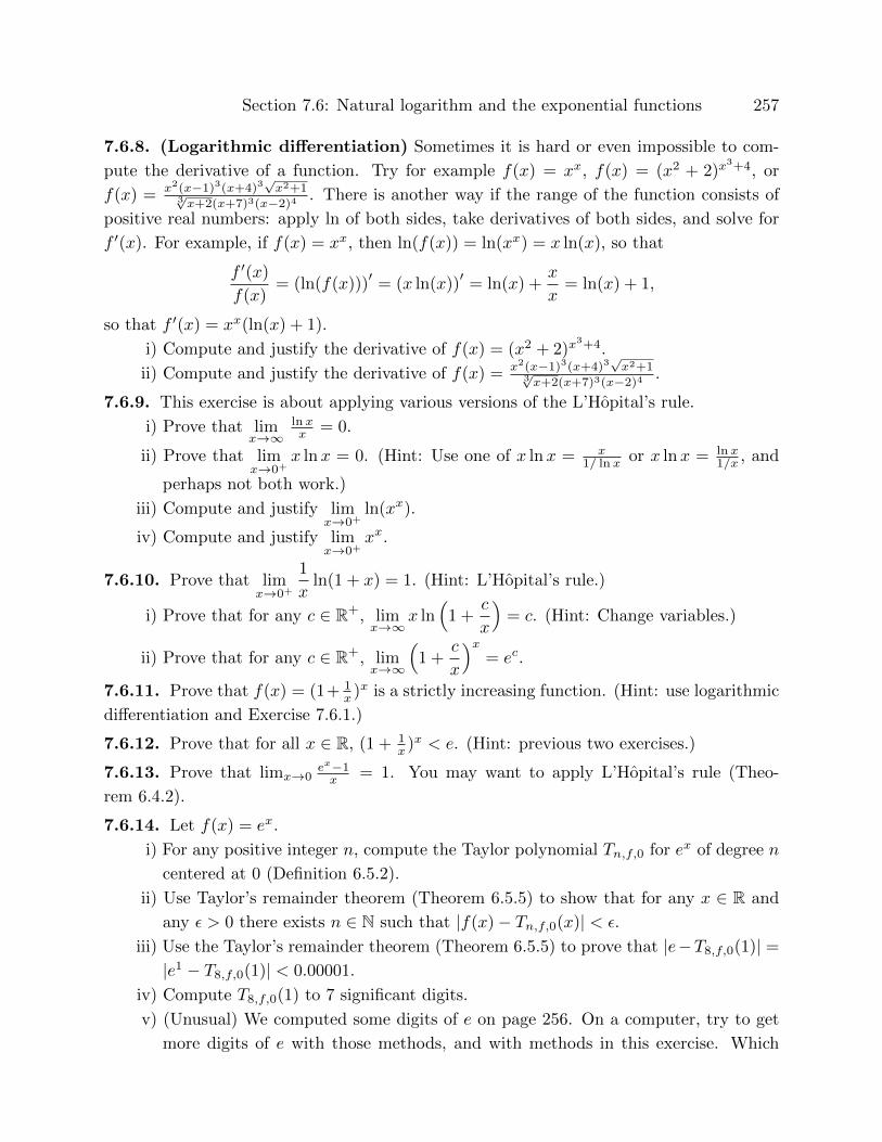
Section 7.6: Natural logarithm and the exponential functions 257
7.6.8. (Logarithmic differentiation) Sometimes it is hard or even impossible to com-
pute the derivative of a function. Try for example f(x) = xx, f(x) = (x2 + 2)x3+4, or
f(x) = x2(x−1)3(x+4)3√x2+1
3√x+2(x+7)3(x−2)4
. There is another way if the range of the function consists of
positive real numbers: apply ln of both sides, take derivatives of both sides, and solve for
f ′(x). For example, if f(x) = xx, then ln(f(x)) = ln(xx) = x ln(x), so that
f ′(x)
f(x)= (ln(f(x)))
′= (x ln(x))
′= ln(x) +
x
x= ln(x) + 1,
so that f ′(x) = xx(ln(x) + 1).
i) Compute and justify the derivative of f(x) = (x2 + 2)x3+4.
ii) Compute and justify the derivative of f(x) = x2(x−1)3(x+4)3√x2+1
3√x+2(x+7)3(x−2)4
.
7.6.9. This exercise is about applying various versions of the L’Hopital’s rule.
i) Prove that limx→∞
ln xx = 0.
ii) Prove that limx→0+
x lnx = 0. (Hint: Use one of x lnx = x1/ ln x or x lnx = ln x
1/x , and
perhaps not both work.)
iii) Compute and justify limx→0+
ln(xx).
iv) Compute and justify limx→0+
xx.
7.6.10. Prove that limx→0+
1
xln(1 + x) = 1. (Hint: L’Hopital’s rule.)
i) Prove that for any c ∈ R+, limx→∞
x ln(
1 +c
x
)= c. (Hint: Change variables.)
ii) Prove that for any c ∈ R+, limx→∞
(1 +
c
x
)x= ec.
7.6.11. Prove that f(x) = (1+ 1x )x is a strictly increasing function. (Hint: use logarithmic
differentiation and Exercise 7.6.1.)
7.6.12. Prove that for all x ∈ R, (1 + 1x )x < e. (Hint: previous two exercises.)
7.6.13. Prove that limx→0ex−1x = 1. You may want to apply L’Hopital’s rule (Theo-
rem 6.4.2).
7.6.14. Let f(x) = ex.
i) For any positive integer n, compute the Taylor polynomial Tn,f,0 for ex of degree n
centered at 0 (Definition 6.5.2).
ii) Use Taylor’s remainder theorem (Theorem 6.5.5) to show that for any x ∈ R and
any ε > 0 there exists n ∈ N such that |f(x)− Tn,f,0(x)| < ε.
iii) Use the Taylor’s remainder theorem (Theorem 6.5.5) to prove that |e−T8,f,0(1)| =|e1 − T8,f,0(1)| < 0.00001.
iv) Compute T8,f,0(1) to 7 significant digits.
v) (Unusual) We computed some digits of e on page 256. On a computer, try to get
more digits of e with those methods, and with methods in this exercise. Which
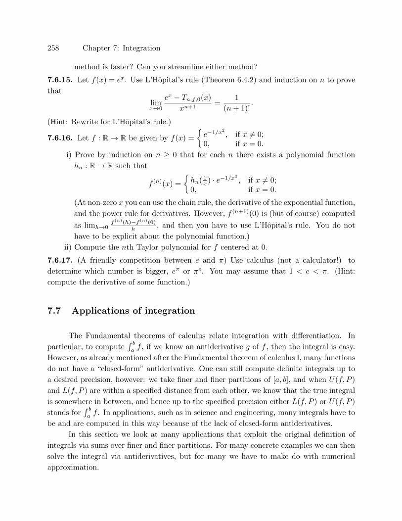
258 Chapter 7: Integration
method is faster? Can you streamline either method?
7.6.15. Let f(x) = ex. Use L’Hopital’s rule (Theorem 6.4.2) and induction on n to prove
that
limx→0
ex − Tn,f,0(x)
xn+1=
1
(n+ 1)!.
(Hint: Rewrite for L’Hopital’s rule.)
7.6.16. Let f : R→ R be given by f(x) =
{e−1/x2
, if x 6= 0;0, if x = 0.
i) Prove by induction on n ≥ 0 that for each n there exists a polynomial function
hn : R→ R such that
f (n)(x) =
{hn( 1
x ) · e−1/x2
, if x 6= 0;0, if x = 0.
(At non-zero x you can use the chain rule, the derivative of the exponential function,
and the power rule for derivatives. However, f (n+1)(0) is (but of course) computed
as limh→0f(n)(h)−f(n)(0)
h , and then you have to use L’Hopital’s rule. You do not
have to be explicit about the polynomial function.)
ii) Compute the nth Taylor polynomial for f centered at 0.
7.6.17. (A friendly competition between e and π) Use calculus (not a calculator!) to
determine which number is bigger, eπ or πe. You may assume that 1 < e < π. (Hint:
compute the derivative of some function.)
7.7 Applications of integration
The Fundamental theorems of calculus relate integration with differentiation. In
particular, to compute∫ baf , if we know an antiderivative g of f , then the integral is easy.
However, as already mentioned after the Fundamental theorem of calculus I, many functions
do not have a “closed-form” antiderivative. One can still compute definite integrals up to
a desired precision, however: we take finer and finer partitions of [a, b], and when U(f, P )
and L(f, P ) are within a specified distance from each other, we know that the true integral
is somewhere in between, and hence up to the specified precision either L(f, P ) or U(f, P )
stands for∫ baf . In applications, such as in science and engineering, many integrals have to
be and are computed in this way because of the lack of closed-form antiderivatives.
In this section we look at many applications that exploit the original definition of
integrals via sums over finer and finer partitions. For many concrete examples we can then
solve the integral via antiderivatives, but for many we have to make do with numerical
approximation.
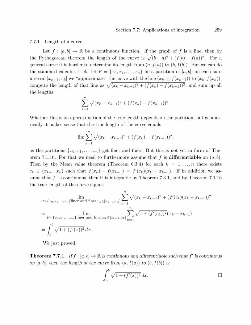
Section 7.7: Applications of integration 259
7.7.1 Length of a curve
Let f : [a, b] → R be a continuous function. If the graph of f is a line, then by
the Pythagorean theorem the length of the curve is√
(b− a)2 + (f(b)− f(a))2. For a
general curve it is harder to determine its length from (a, f(a)) to (b, f(b)). But we can do
the standard calculus trick: let P = {x0, x1, . . . , xn} be a partition of [a, b]; on each sub-
interval [xk−1, xk] we “approximate” the curve with the line (xk−1, f(xk−1)) to (xk, f(xk)),
compute the length of that line as√
(xk − xk−1)2 + (f(xk)− f(xk−1))2, and sum up all
the lengths:n∑k=1
√(xk − xk−1)2 + (f(xk)− f(xk−1))2.
Whether this is an approximation of the true length depends on the partition, but geomet-
rically it makes sense that the true length of the curve equals
limn∑k=1
√(xk − xk−1)2 + (f(xk)− f(xk−1))2,
as the partitions {x0, x1, . . . , xn} get finer and finer. But this is not yet in form of The-
orem 7.1.16. For that we need to furthermore assume that f is differentiable on (a, b).
Then by the Mean value theorem (Theorem 6.3.4) for each k = 1, . . . , n there exists
ck ∈ (xk−1, xk) such that f(xk) − f(xk−1) = f ′(ck)(xk − xk−1). If in addition we as-
sume that f ′ is continuous, then it is integrable by Theorem 7.3.1, and by Theorem 7.1.16
the true length of the curve equals
limP={x0,x1,...,xn}finer and finer,ck∈[xk−1,xk]
n∑k=1
√(xk − xk−1)2 + (f ′(ck)(xk − xk−1))2
= limP={x0,x1,...,xn}finer and finer,ck∈[xk−1,xk]
n∑k=1
√1 + (f ′(ck))2(xk − xk−1)
=
∫ b
a
√1 + (f ′(x))2 dx.
We just proved:
Theorem 7.7.1. If f : [a, b]→ R is continuous and differentiable such that f ′ is continuous
on [a, b], then the length of the curve from (a, f(a)) to (b, f(b)) is∫ b
a
√1 + (f ′(x))2 dx.
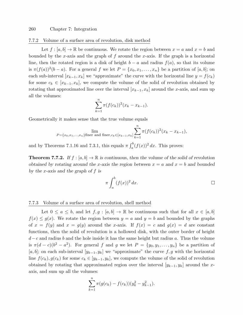
260 Chapter 7: Integration
7.7.2 Volume of a surface area of revolution, disk method
Let f : [a, b]→ R be continuous. We rotate the region between x = a and x = b and
bounded by the x-axis and the graph of f around the x-axis. If the graph is a horizontal
line, then the rotated region is a disk of height b − a and radius f(a), so that its volume
is π(f(a))2(b − a). For a general f we let P = {x0, x1, . . . , xn} be a partition of [a, b]; on
each sub-interval [xk−1, xk] we “approximate” the curve with the horizontal line y = f(ck)
for some ck ∈ [xk−1, xk], we compute the volume of the solid of revolution obtained by
rotating that approximated line over the interval [xk−1, xk] around the x-axis, and sum up
all the volumes:n∑k=1
π(f(ck))2(xk − xk−1).
Geometrically it makes sense that the true volume equals
limP={x0,x1,...,xn}finer and finer,ck∈[xk−1,xk]
n∑k=1
π(f(ck))2(xk − xk−1),
and by Theorems 7.1.16 and 7.3.1, this equals π∫ ba
(f(x))2 dx. This proves:
Theorem 7.7.2. If f : [a, b]→ R is continuous, then the volume of the solid of revolution
obtained by rotating around the x-axis the region between x = a and x = b and bounded
by the x-axis and the graph of f is
π
∫ b
a
(f(x))2 dx.
7.7.3 Volume of a surface area of revolution, shell method
Let 0 ≤ a ≤ b, and let f, g : [a, b] → R be continuous such that for all x ∈ [a, b]
f(x) ≤ g(x). We rotate the region between y = a and y = b and bounded by the graphs
of x = f(y) and x = g(y) around the x-axis. If f(x) = c and g(x) = d are constant
functions, then the solid of revolution is a hollowed disk, with the outer border of height
d−c and radius b and the hole inside it has the same height but radius a. Thus the volume
is π(d − c)(b2 − a2). For general f and g we let P = {y0, y1, . . . , yn} be a partition of
[a, b]; on each sub-interval [yk−1, yk] we “approximate” the curve f, g with the horizontal
line f(ck), g(ck) for some ck ∈ [yk−1, yk], we compute the volume of the solid of revolution
obtained by rotating that approximated region over the interval [yk−1, yk] around the x-
axis, and sum up all the volumes:
n∑k=1
π(g(ck)− f(ck))(y2k − y2
k−1).
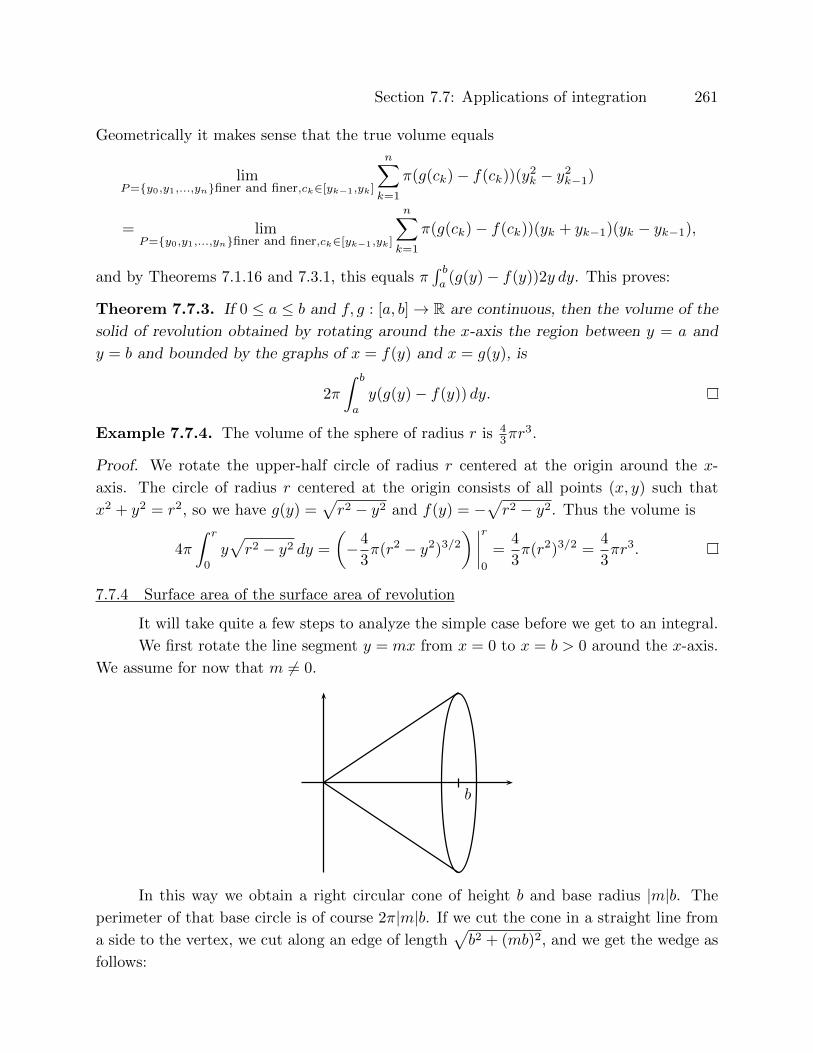
Section 7.7: Applications of integration 261
Geometrically it makes sense that the true volume equals
limP={y0,y1,...,yn}finer and finer,ck∈[yk−1,yk]
n∑k=1
π(g(ck)− f(ck))(y2k − y2
k−1)
= limP={y0,y1,...,yn}finer and finer,ck∈[yk−1,yk]
n∑k=1
π(g(ck)− f(ck))(yk + yk−1)(yk − yk−1),
and by Theorems 7.1.16 and 7.3.1, this equals π∫ ba
(g(y)− f(y))2y dy. This proves:
Theorem 7.7.3. If 0 ≤ a ≤ b and f, g : [a, b]→ R are continuous, then the volume of the
solid of revolution obtained by rotating around the x-axis the region between y = a and
y = b and bounded by the graphs of x = f(y) and x = g(y), is
2π
∫ b
a
y(g(y)− f(y)) dy.
Example 7.7.4. The volume of the sphere of radius r is 43πr
3.
Proof. We rotate the upper-half circle of radius r centered at the origin around the x-
axis. The circle of radius r centered at the origin consists of all points (x, y) such that
x2 + y2 = r2, so we have g(y) =√r2 − y2 and f(y) = −
√r2 − y2. Thus the volume is
4π
∫ r
0
y√r2 − y2 dy =
(−4
3π(r2 − y2)3/2
) ∣∣∣∣r0
=4
3π(r2)3/2 =
4
3πr3.
7.7.4 Surface area of the surface area of revolution
It will take quite a few steps to analyze the simple case before we get to an integral.
We first rotate the line segment y = mx from x = 0 to x = b > 0 around the x-axis.
We assume for now that m 6= 0.
b
In this way we obtain a right circular cone of height b and base radius |m|b. The
perimeter of that base circle is of course 2π|m|b. If we cut the cone in a straight line from
a side to the vertex, we cut along an edge of length√b2 + (mb)2, and we get the wedge as
follows:

262 Chapter 7: Integration
perimeter 2π|m|b
radius√b2 + (mb)2
Without the clip in the disc, the perimeter would be 2π√b2 + (mb)2, but our perime-
ter is only 2π|m|b. Thus the angle subtended by the wedge is by proportionality equal to2π|m|b
2π√b2+(mb)2
2π = 2π|m|√1+m2
. The area of the full circle is radius squared times one half of
the full angle, and so proportionally the area of our wedge is radius squared times one half
of our angle, i.e., the surface area of this surface of revolution is (√b2 + (mb)2)2 2π|m|
2√
1+m2
= π|m|b2√
1 +m2. Note that even if b < 0, the surface area is the absolute value of
πmb2√
1 +m2.
Thus if m is not zero and 0 ≤ a < b or a < b ≤ 0, then the surface area of revolution
obtained by rotating the line y = mx from x = a to x = b equals the absolute value of
πm(b2 − a2)√
1 +m2. Note the geometric requirement that at a and b the line is on the
same side of the x-axis.
Now suppose that we rotate the line y = mx + l around the x-axis, with m 6= 0
and a < b and both on the same side of the intersection of the line with the x-axis. This
intersection is at x = −l/m. By shifting the graph by l/m to the right, this is the same as
rotating the line y = mx from x = a + l/m to x = b + l/m, and by the previous case the
surface area of this is the absolute value of
πm((b+ l/m)2 − (a+ l/m)2)√
1 +m2
= πm(b2 + 2bl/m+ l2/m2 − (a2 + 2al/m+ l2/m2)
)√1 +m2
= πm(b2 − a2 + 2(b− a)l/m
)√1 +m2
= πm(b− a)(b+ a+ 2l/m)√
1 +m2
= π(b− a)(m(b+ a) + 2l)√
1 +m2.
If instead we rotate the line y = l (with m = 0) around the x-axis, we get a ring whose
surface area is (b− a)2π|l|, which is the absolute value of π(b− a)(m(b+ a) + 2l)√
1 +m2.
Thus for all m, the surface area of the surface of revolution obtained by rotating the line
y = mx+ l from x = a to x = b around the x-axis is the absolute value of
π(b− a)(m(b+ a) + 2l)√
1 +m2,

Section 7.7: Applications of integration 263
with the further restriction in case m 6= 0 that a and b are both on the same side of the
x-intercept.
Now let f : [a, b]→ R≥0 be a differentiable (and not necessarily linear) function. Let
P = {x0, x1, . . . , xn} be a partition of [a, b]; on each sub-interval [xk−1, xk] we approximate
the curve with the line from (xk−1, f(xk−1)) to (xk, f(xk)). By the assumption that f
takes on only non-negative values we have that both xk−1, xk are both on the same side of
the x-intercept of that line. The equation of the line is y = f(xk)−f(xk−1)xk−xk−1
(x− xk) + f(xk),
so that m = f(xk)−f(xk−1)xk−xk−1
and l = − f(xk)−f(xk−1)xk−xk−1
xk + f(xk). Since f is differentiable, by
the Mean value theorem (Theorem 6.3.4) there exists ck ∈ (xk−1, xk) such that f ′(ck) =f(xk)−f(xk−1)
xk−xk−1. Thus m = f ′(ck) and l = f(xk)− f ′(ck)xk.
We rotate that line segment around the x-axis, compute its volume of that solid of
revolution, and add up the volumes for all the subparts:
n∑k=1
∣∣∣π(xk − xk−1) (f ′(ck)(xk + xk−1) + 2 (f(xk)− f ′(ck)xk))√
1 + (f ′(ck))2∣∣∣
=
n∑k=1
π |(f ′(ck)(−xk + xk−1) + 2f(xk))|√
1 + (f ′(ck))2(xk − xk−1).
By Theorems 7.1.16 and 7.3.1 we get the following:
Theorem 7.7.5. If f : [a, b] → R≥0 is differentiable with continuous derivative, then the
surface area of the solid of revolution obtained by rotating around the x-axis the curve
y = f(x) between x = a and x = b is
π
∫ b
a
|f ′(x)(−x+ x) + 2f(x)|√
1 + (f ′(x))2 dx = 2π
∫ b
a
f(x)√
1 + (f ′(x))2 dx.
Exercises for Section 7.7
7.7.1. Use the methods from this section to compute the following:
i) The perimeter of the circle.
ii) The volume of the sphere of radius r.
iii) The volume of the ellipsoid whose boundary satisfies x2
a2 + y2
b2 + z2
b2 = 1. (We need
multi-variable calculus to be able to compute the volume of the ellipsoid whose
boundary satisfies x2
a2 + y2
b2 + z2
c2 = 1.)
iv) The volume of a conical pyramid with base radius r and height h.
v) The volume of a doughnut (you specify its dimensions).
vi) The surface area of the sphere of radius r.
264 Chapter 7: Integration
7.7.2. The moment of inertia of a tiny particle of mass m rotating around a circle of radius
r is I = mr2. Likewise, the moment of inertia of a (circular) hoop of radius r and of mass
m rotating around its center is I = mr2. The goal of this exercise is to derive the moment
of inertia of a thin circular plate of radius 5a meters and mass 4 kilograms rotating about
its diameter. (Let b be the thickness of the plate and ρ the mass divided by the volume.)
i) Center the plate at the origin. Let the axis of rotation be the y-axis.
ii) Let P be a partition of [0, 5]. Prove that the moment of inertia of the sliver of
the plate between xk−1 and xk is approximately 452
√x2k − x2
k−1c2k, where ck ∈
[xk−1, xk].
iii) Prove that the moment of inertia of the rotating circular plate is 50 kilogram meters
squared.
7.7.3. If a constant force F moves an object by d units, the work done is W = Fd. Suppose
that F depends on the position as F (x) = kx for some constant k. Find the total work
done between x = a and x = b.
7.7.4. In hydrostatics, (constant) force equals (constant) pressure times (constant) area,
and (constant) pressure equals the weight density of the water w times (constant) depth
h below the surface. But most of the time we do not have tiny particles but large objects
where depth, pressure, and surface areas vary. For example, an object is completely sub-
merged under water from depth a to depth b. At depth h, the cross section area of the
object is A(h). Compute the total force exerted on the object by the water.
Chapter 8: Sequences
In this chapter, Sections 8.5 and 8.4 contain identical results in identical order, but
the proofs are different. You may want to learn both perspectives, or you may choose to
omit one of the two sections.
8.1 Introduction to sequences
Definition 8.1.1. An infinite sequence is a function with domain N+ and codomain C.
If s is such a function, instead of writing s(n), it is common to write sn, and the sequence
s is commonly expressed also in all of the following notations (and obviously many more):
s = {s1, s2, s3, . . .} = {sn}∞n=1 = {sn}n≥1 = {sn}n = {sn+3}∞n=−2 = {sn−4}n>4 = {sn}.
The nth element sn = s(n) in the ordered list is called the nth term of the sequence.
The notation {s1, s2, s3, . . .} usually stands for the set consisting of the elements
s1, s2, s3, . . ., and the order of a listing of elements in a set is irrelevant. Here, however,
{s1, s2, s3, . . .} stands for the sequence, and the order matters. When the usage is not
clear from the context, we add the word “sequence” or “set” as appropriate.
The first term of the sequence {2n− 1}n≥4 is 7, the second term is 9, et cetera. The
point is that even though the notating of a sequence can start with an arbitrary integer,
the counting of the terms always starts with 1.
Note that sn is the nth term of the sequence s, whereas {sn} = {sn}n≥1 is the
sequence in which n plays a dummy variable. Thus
s = {sn} 6= sn.
Examples and notation 8.1.2.
(1) The terms of a sequence need not be distinct. For any complex number c, {c} =
{c, c, c, . . .} is called a constant sequence.
(2) For any complex numbers c and d, the sequence {c, d, c, d, c, d, . . .} can be written
more concisely as {d−c2 (−1)n + c+d2 }n.
(3) The sequence {(−1)n} = {−1, 1,−1, 1, . . .} has an infinite number of terms, and
its range is the finite set {−1, 1}. The range of the sequence {in} is the set
{i,−1,−i, 1}.

266 Chapter 8: Sequences
(4) The sequence s with s(n) = n + 4 for all n ≥ 1 can be written as {n + 4} =
{n+ 4}n≥1 = {5, 6, 7, . . .} = {n}n≥5. This sequence is different from the sequence
{n} = {1, 2, 3, . . .}.(5) The sequence {2n} is an abbreviation for the sequence {2, 4, 6, 8, . . .}. This is not
the same as the sequence {4, 2, 8, 6, 12, 10, . . .}, namely, if we scramble the order
of the terms, we change the sequence.
(6) The sequence of all odd positive integers (in the natural order) can be written as
{2n− 1} = {2n− 1}n≥1 = {2n+ 1}n≥0 (and in many other ways).
(7) Terms of a sequence can be defined recursively. For example, let s1 = 1, and for
each n ≥ 1 let sn+1 = 2sn. Then the sequence of these sn has a non-recursive form
sn = 2n−1. If however, s1 = 1 and for each n ≥ 1, sn+1 = 2s3n+√sn + 2+ln(sn)+1,
then we can certainly compute any one sn by invoking sk for k < n, but we will
not get a closed-form for sn as in the previous example.
(8) (Fibonacci numbers) Let s1 = 1, s2 = 1, and for all n ≥ 2, let sn+1 = sn+sn−1.
This sequence starts with 1, 1, 2, 3, 5, 8, 13, 21, 34, . . ., and obviously keeps growing.
(For more on these numbers, see Exercise 1.5.30, where in particular it is proved
that for all integers n, sn = 1√5
(1+√
52
)n− 1√
5
(1−√
52
)n.)
(9) Some sequences, just like functions, do not have an algebraic expression for terms.
For example, let s be the sequence whose nth term is the nth prime number.
This sequence starts with 2, 3, 5, 7, 11, 13, 17, 19, 23, and we could write many more
terms out explicitly, but we do not have a formula for them. (This s is indeed an
infinite sequence since there are infinitely many primes, as proved on page 32.)
(10) Note that {n}n∈Z is NOT a sequence because the list has no first term.
(11) However, one can scramble the set Z of all integers into a sequence. One way
of doing this as as follows: {0, 1,−1, 2,−2, 3,−3, 4,−4, . . .}, which algebraically
equals
sn =
{n/2, if n is even;−(n− 1)/2, otherwise.
(“Otherwise” applies to odd (positive) integers.)
(12) One can scramble the set Q+ of all positive rational numbers into a sequence via
a diagonal construction as follows. First of all, each positive rational number can
be written in the form a/b for some positive integers a, b. Rather than plotting the
fraction a/b, we will plot the point (a, b) in the plane. Refer to Plot 8.1.2: the bold
points are elements of N+×N+, and each such (a, b) is identified with the fraction
a/b. Every positive rational number appears in this way somewhere as a bold point,
and all appear multiple times because ab = ac
bc . Now we want to systematically
enumerate these bold points/rational numbers. If we first enumerate all of them
in the first row, and then proceed to the second row, well, actually, we never get
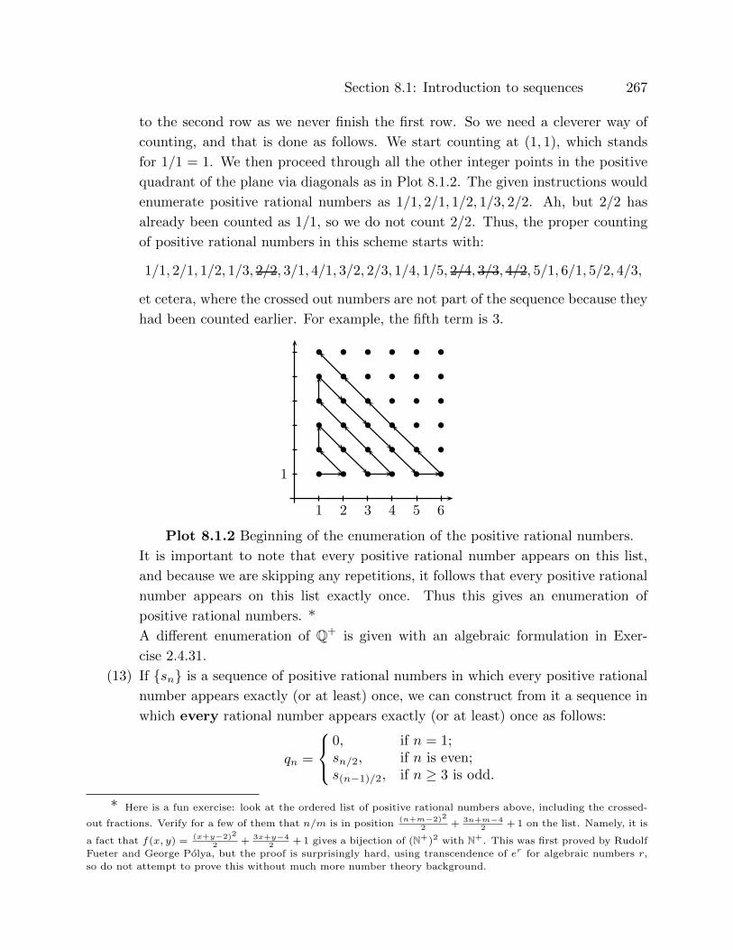
Section 8.1: Introduction to sequences 267
to the second row as we never finish the first row. So we need a cleverer way of
counting, and that is done as follows. We start counting at (1, 1), which stands
for 1/1 = 1. We then proceed through all the other integer points in the positive
quadrant of the plane via diagonals as in Plot 8.1.2. The given instructions would
enumerate positive rational numbers as 1/1, 2/1, 1/2, 1/3, 2/2. Ah, but 2/2 has
already been counted as 1/1, so we do not count 2/2. Thus, the proper counting
of positive rational numbers in this scheme starts with:
1/1, 2/1, 1/2, 1/3, 2/2, 3/1, 4/1, 3/2, 2/3, 1/4, 1/5, 2/4, 3/3, 4/2, 5/1, 6/1, 5/2, 4/3,
et cetera, where the crossed out numbers are not part of the sequence because they
had been counted earlier. For example, the fifth term is 3.
1
1 2 3 4 5 6
�
�
�
�
�
�
�
�
�
�
�
�
�
�
�
�
�
�
�
�
�
�
�
�
�
�
�
�
�
�
�
�
�
�
�
�
Plot 8.1.2 Beginning of the enumeration of the positive rational numbers.
It is important to note that every positive rational number appears on this list,
and because we are skipping any repetitions, it follows that every positive rational
number appears on this list exactly once. Thus this gives an enumeration of
positive rational numbers. *
A different enumeration of Q+ is given with an algebraic formulation in Exer-
cise 2.4.31.
(13) If {sn} is a sequence of positive rational numbers in which every positive rational
number appears exactly (or at least) once, we can construct from it a sequence in
which every rational number appears exactly (or at least) once as follows:
qn =
0, if n = 1;sn/2, if n is even;s(n−1)/2, if n ≥ 3 is odd.
* Here is a fun exercise: look at the ordered list of positive rational numbers above, including the crossed-
out fractions. Verify for a few of them that n/m is in position(n+m−2)2
2 + 3n+m−42 + 1 on the list. Namely, it is
a fact that f(x, y) =(x+y−2)2
2 + 3x+y−42 + 1 gives a bijection of (N+)2 with N+. This was first proved by Rudolf
Fueter and George Polya, but the proof is surprisingly hard, using transcendence of er for algebraic numbers r,
so do not attempt to prove this without much more number theory background.
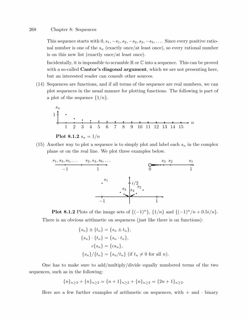
268 Chapter 8: Sequences
This sequence starts with 0, s1,−s1, s2,−s2, s3,−s3, . . .. Since every positive ratio-
nal number is one of the sn (exactly once/at least once), so every rational number
is on this new list (exactly once/at least once).
Incidentally, it is impossible to scramble R or C into a sequence. This can be proved
with a so-called Cantor’s diagonal argument, which we are not presenting here,
but an interested reader can consult other sources.
(14) Sequences are functions, and if all terms of the sequence are real numbers, we can
plot sequences in the usual manner for plotting functions. The following is part of
a plot of the sequence {1/n}.
�
�� � � � � � � � � � � � �
1
1 2 3 4 5 6 7 8 9 10 11 12 13 14 15
sn
n
Plot 8.1.2 sn = 1/n
(15) Another way to plot a sequence is to simply plot and label each sn in the complex
plane or on the real line. We plot three examples below.
1−1
s2, s4, s6, . . .s1, s3, s5, . . . s1s2s3
10
�
��
�� �� �� �� �� �� �� �� �
s1
s2s3 s4
−1 1
i/2
Plot 8.1.2 Plots of the image sets of {(−1)n}, {1/n} and {(−1)n/n+ 0.5i/n}.There is an obvious arithmetic on sequences (just like there is on functions):
{sn} ± {tn} = {sn ± tn},{sn} · {tn} = {sn · tn},
c{sn} = {csn},{sn}/{tn} = {sn/tn} (if tn 6= 0 for all n).
One has to make sure to add/multiply/divide equally numbered terms of the two
sequences, such as in the following:
{n}n≥3 + {n}n≥2 = {n+ 1}n≥2 + {n}n≥2 = {2n+ 1}n≥2.
Here are a few further examples of arithmetic on sequences, with + and · binary
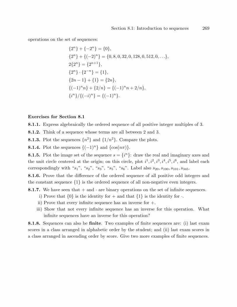
Section 8.1: Introduction to sequences 269
operations on the set of sequences:
{2n}+ {−2n} = {0},{2n}+ {(−2)n} = {0, 8, 0, 32, 0, 128, 0, 512, 0, . . .},2{2n} = {2n+1},{2n} · {2−n} = {1},{2n− 1}+ {1} = {2n},{(−1)nn}+ {2/n} = {(−1)nn+ 2/n},{in}/{(−i)n} = {(−1)n}.
Exercises for Section 8.1
8.1.1. Express algebraically the ordered sequence of all positive integer multiples of 3.
8.1.2. Think of a sequence whose terms are all between 2 and 3.
8.1.3. Plot the sequences {n2} and {1/n2}. Compare the plots.
8.1.4. Plot the sequences {(−1)n} and {cos(nπ)}.8.1.5. Plot the image set of the sequence s = {in}: draw the real and imaginary axes and
the unit circle centered at the origin; on this circle, plot i1, i2, i3, i4, i5, i6, and label each
correspondingly with “s1”, “s2”, “s3”, “s5”, “s6”. Label also s20, s100, s101, s345.
8.1.6. Prove that the difference of the ordered sequence of all positive odd integers and
the constant sequence {1} is the ordered sequence of all non-negative even integers.
8.1.7. We have seen that + and · are binary operations on the set of infinite sequences.
i) Prove that {0} is the identity for + and that {1} is the identity for ·.ii) Prove that every infinite sequence has an inverse for +.
iii) Show that not every infinite sequence has an inverse for this operation. What
infinite sequences have an inverse for this operation?
8.1.8. Sequences can also be finite. Two examples of finite sequences are: (i) last exam
scores in a class arranged in alphabetic order by the student; and (ii) last exam scores in
a class arranged in ascending order by score. Give two more examples of finite sequences.

270 Chapter 8: Sequences
8.2 Convergence of infinite sequences
Definition 8.2.1. A sequence s = {sn} converges to L ∈ C if for every real number
ε > 0 there exists a positive real number N such that for all integers n > N , |sn − L| < ε.
If s converges to L, we also say that L is the limit of {sn}. We use the following
notations for this:
sn → L, {sn} → L,
lim s = L, lim sn = L, lim{sn} = L, lim(sn) = L,
limn→∞
sn = L, limn→∞
{sn} = L, limn{sn} = L, lim
n→∞(sn) = L,
and, to save vertical space, just like for limits of functions, we also use a variation on the
last three: limn→∞ sn = L, limn→∞{sn} = L, limn→∞(sn) = L.
We say that a sequence is convergent it it has a limit.
For example, the constant sequence s = {c} converges to L = c because for all n,
|sn − L| = |c− c| = 0 is strictly smaller than any positive real number ε.
The sequence s = {300,−5, π, 4, 0.5, 106, 2, 2, 2, 2, 2, . . .} converges to L = 2 because
for all n ≥ 7, |sn − L| = |2− 2| = 0 is strictly smaller than any positive real number ε.
In conceptual terms, a sequence {sn} converges if the tail end of the sequence gets
closer and closer to L; you can make all sn with n > N get arbitrarily close to L by simply
increasing N a sufficient amount.
We work out examples of epsilon-N proofs; they are similar to the epsilon-delta
proofs, and we go through them slowly at first. Depending on the point of view of your
class, the reader may wish to skip the rest of this section for an alternative treatment
in Section 8.5 in terms of limits of functions. More epsilon-N proofs are in Section 8.4.
Be aware that this section is more concrete; the next section assumes greater ease with
abstraction.
Example 8.2.2. Consider the sequence s = {1/n}. Example 8.1.2 gives a hunch that
lim sn = 0, and now we prove it. [(Recall that any text between square brackets
in this font and in red color is what should approximately be going through
your thoughts, but it is not something to write down in a final solution.)
By the definition of convergence, we have to show that for all ε > 0 some
property holds. All proofs of this form start with:] Let ε be an arbitrary
positive number. [Now we have to show that there exists an N for which
some other property holds. Thus we have to construct an N . Usually
this is done in retrospect, one cannot simply guess an N , but in the final
write-up, readers see simply that educated guess – more about how to guess
educatedly later:] Set N = 1ε . Then N is a positive real number. [Now we have to

Section 8.2: Convergence of infinite sequences 271
show that for all integers n > N , |sn − 0| < ε. All proofs of statements of
the form “for all integers n > N” start with:] Let n be an (arbitrary) integer
with n > N . [Finally, we have to prove the inequality |sn− 0| < ε. We do that
by algebraically manipulating the left side until we get the desired final
< ε:]
|sn − 0| = |1/n− 0|= |1/n|= 1/n (because n is positive)
< 1/N (because n > N > 0)
=1
(1/ε)(because N = 1/ε) [Ah, what a clever guess that was!]
= ε.
So we conclude that |sn − 0| < ε, which proves that lim sn = 0.
Just as in the epsilon-delta proofs where one has to find a δ, similarly how does one
divine an N? In the following two examples we indicate this step-by-step, not as a book
or your final homework solution would have it recorded.
Example 8.2.3. Let sn = { 1n ((−1)n + i(−1)n+1)}. If we write out the first few terms, we
find that {sn} = {−1+ i, 1/2− i/2,−1/3+ i/3, . . .}, and we may speculate that lim sn = 0.
Here is plot of the image set of this sequence in the complex plane:
�
�
�
�
�
�
�
�
�
�
��
��
��
��
��
s1
s2
s3
s4−1 1
i/2
We prove that lim sn = 0. Let ε > 0. Set N = . [We will eventually
fill in what the positive real number N should be, but at this point of the
proof simply leave some blank space. Assuming that N is in place, we next
need to prove that for every integer n > N , the relevant property as in
the ε−N definition of limits holds. The proof of “for every integer n > N”
always starts with:] Let n be an integer strictly bigger than N . [We want to make
sure eventually that n is positive, which is guaranteed if N is positive, but
with blank N , we will simply assume in the algebra below that N is positive.]
Then
|sn − 0| =∣∣∣∣ 1n ((−1)n + i(−1)n+1)− 0
∣∣∣∣
272 Chapter 8: Sequences
=
∣∣∣∣ 1n∣∣∣∣ · |(−1)n + i(−1)n+1| (because |ab| = |a||b|)
=1
n· |(−1)n + i(−1)n+1| (because n is positive)
=1
n·√
((−1)n)2 + ((−1)n+1)2
=1
n·√
2
<1
N·√
2 (because n > N)
[Aside: we want/need√
2/N ≤ ε, and√
2/N = ε is a possibility, so set N =√
2/ε.
Now go ahead, write that missing information on N in line 1 of this proof!]
=
√2√
2/ε(because N =
√2/ε)
= ε,
which proves that for all n > 1/ε, |sn − 0| < ε. Since ε is arbitrary, this proves that
lim sn = 0.
Thus a polished version of the example just worked out looks like this:
We prove that lim{
1n ((−1)n + i(−1)n+1)− 0
}= 0. Let ε > 0. Set N =
√2/ε. Then
N is a positive real number. Let n be an integer strictly bigger than N . Then
|sn − 0| =∣∣∣∣ 1n ((−1)n + i(−1)n+1)− 0
∣∣∣∣=
∣∣∣∣ 1n∣∣∣∣ · |(−1)n + i(−1)n+1| (because |ab| = |a||b|)
=1
n· |(−1)n + i(−1)n+1| (because n is positive)
=1
n·√
((−1)n)2 + ((−1)n+1)2
=1
n·√
2
<1
N·√
2 (because n > N)
=
√2√
2/ε(because N =
√2/ε)
= ε,
which proves that for all n >√
2/ε, |sn − 0| < ε. Since ε is arbitrary, this proves that
lim sn = 0.

Section 8.2: Convergence of infinite sequences 273
Example 8.2.4. Claim: lim 2n+3n2
3+4n+n2 = 3. Proof: Let ε > 0. Set N = . Let n be
an integer strictly bigger than N . Then∣∣∣∣ 2n+ 3n2
3 + 4n+ n2− 3
∣∣∣∣ =
∣∣∣∣ 2n+ 3n2
3 + 4n+ n2− 3(3 + 4n+ n2)
3 + 4n+ n2
∣∣∣∣=
∣∣∣∣ −9− 10n
3 + 4n+ n2
∣∣∣∣=
9 + 10n
3 + 4n+ n2(because n > 0) [Assuming that N > 0.]
≤ n+ 10n
3 + 4n+ n2(because n ≥ 9) [Assuming that N ≥ 8.]
=11n
3 + 4n+ n2
≤ 11n
n2(because 3 + 4n+ n2 > n2, so 1/(3 + 4n+ n2) < 1/n2)
=11
n
<11
N(because n > N)
≤ 11
11/ε(because N ≥ 11/ε so 1/N ≤ 1/(11/ε)) [Assuming this.]
= ε,
which was desired. Now (on scratch paper) we gather all the information we used about N :
N > 0, N ≥ 8, N ≥ 11/ε, and that is it. Thus on the first line we fill in the blank part:
Set N = max{8, 11/ε}, which says that N is either 8 or 11/ε, whichever is greater, so that
N ≥ 8 and N ≥ 11/ε.
The polished version of this proof would go as follows:
Example 8.2.5. Claim: lim 2n+3n2
3+4n+n2 = 3. Proof: Let ε > 0. Set N = max{8, 11/ε}. Then
N is a positive real number. Let n be an integer strictly bigger than N . Then∣∣∣∣ 2n+ 3n2
3 + 4n+ n2− 3
∣∣∣∣ =
∣∣∣∣ 2n+ 3n2
3 + 4n+ n2− 3(3 + 4n+ n2)
3 + 4n+ n2
∣∣∣∣=
∣∣∣∣ −9− 10n
3 + 4n+ n2
∣∣∣∣=
9 + 10n
3 + 4n+ n2(because n > 0)
≤ n+ 10n
3 + 4n+ n2(because n ≥ 9)
=11n
3 + 4n+ n2
274 Chapter 8: Sequences
≤ 11n
n2(because 3 + 4n+ n2 > n2, so 1/(3 + 4n+ n2) < 1/n2)
=11
n
<11
N(because n > N)
≤ 11
11/ε(because N ≥ 11/ε so 1/N ≤ 1/(11/ε))
= ε,
which proves that for all n > N , |sn−3| < ε. Since ε is arbitrary, this proves that the limit
of this sequence is 3.
Below is a polished proof of a very similar problem.
Example 8.2.6. Claim: lim −2n+3n2
9−4n+n2 = 3. Proof: Let ε > 0. Set N = max{2, 20/ε}. Then
N is a positive real number. Let n be an integer strictly bigger than N . Then∣∣∣∣ −2n+ 3n2
9− 4n+ n2− 3
∣∣∣∣ =
∣∣∣∣ −2n+ 3n2
9− 4n+ n2− 3(9− 4n+ n2)
9− 4n+ n2
∣∣∣∣=
∣∣∣∣ −27 + 10n
9− 4n+ n2
∣∣∣∣=−27 + 10n
9− 4n+ n2(because n > N ≥ 2, so n ≥ 3, so 10n− 27 > 0,
and n2 − 4n+ 9 = (n− 3)2 + 2n > 0)
<10n
9− 4n+ n2(because 10n− 27 < 10n)
=10n
9− 4n+ (1/√
2)n2 + (1− 1/√
2)n2
<10n
(1− 1/√
2)n2(because 0 < (n− 4)2 + 2 = 2(9− 4n+ (1/
√2)n2))
<10
0.5n(because 1− 1/
√2 > 0.5, so 1
1−1/√
2< 1
0.5 )
=20
n
<20
N(because n > N)
≤ 20
20/ε(because N ≥ 20/ε so 1/N ≤ 1/(20/ε))
= ε,
which proves that for all n > N , |sn−3| < ε. Since ε is arbitrary, this proves that the limit
of this sequence is 3.

Section 8.2: Convergence of infinite sequences 275
Example 8.2.7. Let r ∈ C such that |r| < 1. Then limn→∞ rn = 0.
Proof. If r = 0, the sequence {rn} is the constant zero sequence so certainly the limit is 0.
So we may assume without loss of generality that r 6= 0. Let ε > 0. Set N =ln(min{ε,0.5})
ln |r| . Since ln of numbers between 0 and 1 is negative, we have that N is a positive
number. Let n be an integer with n > N . Then
|rn − 0| = |r|n
= |rn−N | |r|N
< 1n−N |r|N (by Theorem 7.6.5)
= min{ε, 0.5}≤ ε.
Example 8.2.8. lim{(
1 + 1n
)n}= e.
Proof. All the hard work for this has been done already in Exercise 7.6.10. Let ε > 0. By
Exercise 7.6.10, limx→∞{(
1 + 1x
)x}= e. Thus there exists N > 0 such that for all x > N ,∣∣{(1 + 1
x
)x}− e∣∣ < ε. In particular, for any integer n > N ,∣∣{(1 + 1
n
)n}− e∣∣ < ε.
Example 8.2.9. limn1/n = 1.
Proof. For all n ≥ 2, by Exercise 1.6.7,
n = (n1/n)n = (n1/n − 1 + 1)n =n∑k=0
(n
k
)(n1/n − 1)k.
Each of the summands is non-negative, and if we only use the summands with k = 0 and
k = 2, we then get that
n ≥ 1 +1
2n(n− 1)(n1/n − 1)2.
By subtracting 1 we get that n−1 ≥ 12n(n−1)(n1/n−1)2, so that for n ≥ 2, 2
n ≥ (n1/n−1)2,
and hence that√
2√n≥ n1/n − 1. Certainly n1/n − 1 ≥ 0 for all n ≥ 1. It follows that for all
n ≥ 2, and even for all n ≥ 1, 0 ≤ n1/n − 1 ≤√
2√n
. Now let ε > 0. Set N = max{2, 2/ε2}.Then N is a positive real number. Let n > N be an integer. Then 0 ≤ n1/n − 1 ≤
√2√n<
√2√N
= ε, which proves that |n1/n − 1| < ε, and hence proves this limit.

276 Chapter 8: Sequences
Example 8.2.10. Let M be a positive real number. Then limM1/n = 1.
Proof. First suppose that M ≥ 1. Then certainly for all integers n ≥ M , we have that
1 ≤ M1/n ≤ n1/n. Let ε > 0. By the previous example, there exists N > 0 such
that for all integers n > N , 0 < n1/n − 1 < ε. Then for all integers n > max{M,N},0 ≤M1/n − 1 ≤ n1/n − 1 < ε, which implies that |M1/n − 1| < ε. This proves the example
in case M ≥ 1.
Now suppose that M < 1. By assumption, 1/M > 1, so by the previous case
(and by using that (1/M)1/n = 1/M1/n), there exists N > 0 such that for all integers
n > N , 0 ≤ 1/M1/n − 1 < ε. By adding 1 to all three parts in this inequality we get that
1 ≤ 1/M1/n < ε+1, so that by compatibility of < with multiplication by positive numbers,1ε+1 < M1/n ≤ 1. Hence by compatibility of < with addition,
0 ≤ 1−M1/n < 1− 1
ε+ 1=
ε
ε+ 1< ε,
since ε+ 1 > 1. Thus |1−M1/n| < ε, which proves that limM1/n = 1.
Exercises for Section 8.2
8.2.1. Let sn = 1/n2. Fill in the blanks of the following proof that lim{sn} = 0.
Let ε > 0. Set N = . Then if n > N ,
|sn − 0| =∣∣∣∣ 1
n2− 0
∣∣∣∣=
1
n2(because )
<1
N2(because )
= (because )
= ε.
8.2.2. Prove that for any real number L, lim{ 1n + L} = L.
8.2.3. Prove that for any positive real number k, lim{1/nk} = 0.
8.2.4. Prove that lim sin(n)n = 0.
8.2.5. Prove that lim 2n+1n2−4 = 0.
8.2.6. Prove that lim 3n+42n = 3
2 .
8.2.7. Prove that lim{√
n+ 1−√n}
= 0.
8.2.8. Prove that for every positive integer k, lim{√
n+ k −√n}
= 0.

Section 8.3: Divergence of infinite sequences and infinite limits 277
8.2.9. Suppose that the terms of a sequence are given by sn =∑nk=1
1k(k+1) .
i) Using induction on n, prove that∑nk=1
1k(k+1) = 1− 1
n+1 .
ii) Use this to find and prove the limit of {sn}.
8.2.10. Prove the following limits:
i) lim ln(n)ln(n+1) = 1. (Hint: epsilon-N proof, continuity of ln.)
ii) lim ln(ln(n))ln(ln(n+1)) = 1.
8.2.11. Let r ∈ R. By ‘thmratlbetween’, for every positive integer n, there exists a
rational number sn ∈ (r − 1n , r + 1
n ). Prove that {sn} converges to r.
8.2.12. Let r be a real number with a known decimal expansion. Let sn be the rational
number whose digits n+ 1, n+ 2, n+ 3, et cetera, beyond the decimal point are all 0, and
all other digits agree with the digits of r. (For example, if r = π, then s1 = 3.1, s2 = 3.14,
s7 = 3.1415926, et cetera.) Prove that lim{sn} = r. (Repeat with binary expansions if you
know what a binary expansion is.)
8.2.13. Prove that limn{ n!√n! } = 1.
8.2.14. What is wrong with the following “proof” that limn→∞n
2n+1 = 12 .
“Proof.” Let ε > 0. Set N =12ε−1
2 . Let n > N . Then∣∣∣∣ n
2n+ 1− 1
2
∣∣∣∣ =
∣∣∣∣2n− (2n+ 1)
2(2n+ 1)
∣∣∣∣=
∣∣∣∣ −1
2(2n+ 1)
∣∣∣∣=
1
2(2n+ 1)
<1
2(2N + 1)(because all terms are positive)
= ε.
8.3 Divergence of infinite sequences and infinite limits
The sequence {(−1)n} alternates in value between −1 and 1, and does not seem to
converge to a single number. The following definition addresses this situation.
278 Chapter 8: Sequences
Definition 8.3.1. A sequence diverges if it does not converge. In other words, {sn}diverges if for all complex numbers L, lim{sn} 6= L.
By the usual negation of statements (see chart on page 32), lim{sn} 6= L means:
not(For all real numbers ε > 0 there exists a positive real number
N such that for all integers n > N , |sn − L| < ε.)
= There exists a real number ε > 0 such that not(
there exists
a positive real number N such that for all integers n > N ,
|sn − L| < ε.)
= There exists a real number ε > 0 such that for all positive real
numbers N , not(
for all integers n > N , |sn − L| < ε.)
= There exists a real number ε > 0 such that for all positive real
numbers N there exists an integer n > N such that not(
|sn − L| < ε.)
= There exists a real number ε > 0 such that for all positive
real numbers N there exists an integer n > N such that
|sn − L| ≥ ε.
Example 8.3.2. {(−1)n} is divergent. Namely, for all complex numbers L, lim sn 6= L.
Proof. Set ε = 1 (half the distance between the two values of the sequence). Let N be
an arbitrary positive number. If Re(L) > 0, let n be an odd integer greater than N ,
and if Re(L) ≤ 0, let n be an even integer greater than N . In either case, |sn − L| ≥|Re(sn)− Re(L)| ≥ 1 = ε.
The sequence in the previous example has no limit, whereas the sequence in the next
example has no finite limit:
Example 8.3.3. For all complex numbers L, lim{n} 6= L.
Proof. Set ε = 53 (any positive number will work). Let N be a positive real number. Let n
be any integer that is strictly bigger than N and strictly bigger than |L|+ 53 (say strictly
bigger than N + |L|+ 53). Such an integer exists. Then by the reverse triangle inequality,
|n− L| ≥ |n| − |L| ≥ 53 = ε.
The last two examples are different: the first one has no limit at all since the terms
oscillate wildly, but for the second example we have a sense that its limit is infinity. We
formalize this:
Section 8.3: Divergence of infinite sequences and infinite limits 279
Definition 8.3.4. A real-valued sequence {sn} diverges to ∞ if for every positive real
number M there exists a positive number N such that for all integers n > N , sn > M . We
write this as lim sn =∞.
A real-valued sequence {sn} diverges to −∞ if for every negative real number M
there exists a positive real number N such that for all integers n > N , sn < M . We write
this as lim sn = −∞.
Example 8.3.5. limn =∞.
Proof. Let M > 0. Set N = M . (As in epsilon-delta or epsilon-N proofs, we must figure
out what to set N to. In this case, N = M works). Let n ∈ N+ with n > N . Since N = M ,
we conclude that n > M , and the proof is complete.
Example 8.3.6. lim n√n! =∞.
Proof. Let M > 0. Let M0 be an integer that is strictly greater than M . By Example 8.2.10
there exists N1 > 0 such that for all integers n > N1,∣∣∣∣∣ n√
M0!
(M0 + 1)M0− 1
∣∣∣∣∣ < M0 + 1−MM0 + 1
.
Since M0! = M0(M0 − 1)(M0 − 2) · · · 3 · 2 · 1 < (M0 + 1)M0 , this means that
0 ≤ 1− n
√M0!
(M0 + 1)M0<M0 + 1−MM0 + 1
= 1− M
M0 + 1,
so that n
√M0!
(M0+1)M0> M
M0+1 . Set N = max{N1,M0}. Then for all integers n > N ,
n! = n(n− 1) · · · (M0 + 1) ·M0! ≥ (M0 + 1)n−M0 ·M0! = (M0 + 1)nM0!
(M0 + 1)M0,
so that
n√n! ≥ (M0 + 1) n
√M0!
(M0 + 1)M0> (M0 + 1)
M
M0 + 1= M.
Theorem 8.3.7. (Comparison theorem (for sequences with infinite limits)) Let
{sn}, {tn} be real-valued sequences such that for all sufficiently large n (say for n ≥ N for
some fixed N), sn ≤ tn.
(1) If lim sn =∞, then lim tn =∞.
(2) If lim tn = −∞, then lim sn = −∞.
Proof. (1) By assumption lim sn =∞ for every positive M there exists a positive N ′ such
that for all integers n > N ′, sn > M . Hence by assumption tn ≥ sn for all n ≥ N we get
280 Chapter 8: Sequences
that for every positive M and for all integers n > max{N,N ′}, tn > M . Thus by definition
lim tn =∞.
Part (2) has an analogous proof.
Example 8.3.8. lim n2+1n =∞.
Proof. Note that for all n ∈ N+, n2+1n = n + 1
n ≥ n, and since we already know that
limn =∞, it follows by the comparison theorem above that lim n2+1n =∞.
Example 8.3.9. lim n2−1n =∞.
Proof. Note that for all integers n > 2, n2−1n = n − 1
n ≥n2 . We already know that
limn = ∞, and it is straightforward to prove that lim n2 = ∞. Hence by the comparison
theorem, lim n2−1n =∞.
Or, we can give an M − N proof. Let M > 0. Set N = max{2, 2M}. Let n be an
integer strictly bigger than N . Then
n2 − 1
n= n− 1
n≥ n
2>N
2≥M.
Theorem 8.3.10. Let {sn} be a sequence of positive numbers. Then lim sn = ∞ if and
only if lim 1sn
= 0.
Proof. Suppose that lim sn = ∞. Let ε > 0. By the definition of infinite limits, there
exists a positive number N such that for all integers n > N , sn > 1/ε. Then for the same
n, 0 < 1sn< ε, so that | 1
sn| < ε. This proves that lim 1
sn= 0.
Now suppose that lim 1sn
= 0. Let M be a positive number. By assumption lim 1sn
=
0 there exists a positive number N such that for all integers n > N , | 1sn− 0| < 1/M . Since
each sn is positive, it follows that for the same n, 1sn< 1/M , so that sn > M . This proves
that lim sn =∞.
Exercises for Section 8.3
8.3.1. Prove that the following sequences diverge:
i) {√n}.
ii) {2√n}.
iii) {(n+ 1)3 − n3}.iv) {(−1)n + 3/n}.
8.3.2. Suppose that {sn} diverges and {tn} converges. Prove that {sn ± tn} diverges.
8.3.3. Suppose that {sn} diverges and {tn} converges to a non-zero number. Prove that
{sn · tn} diverges.
Section 8.4: Convergence theorems via epsilon-N proofs 281
8.3.4. Give an example of two divergent sequences {sn}, {tn} such that {sn+tn} converges.
8.3.5. Let {sn} be a sequence of negative numbers. Prove that lim sn = −∞ if and only
if lim 1sn
= 0.
8.3.6. Given the following sequences, find and prove the limits, finite or infinite, if they
exist. Otherwise, prove divergence:
i) { n+5n3−5}.
ii) { 2n2−n3n2−5 }.
iii) { (−1)n
n−3 }.iv) { (−1)nn
n+1 }.v) {n
3−8nn2+8n}.
vi) { 1−n2
n }.vii) { 2n
n! }.viii) { n!
(n+1)!}.
8.3.7. Prove or give a counterexample:
i) If {sn} and {tn} both diverge, then {sn + tn} diverges.
ii) If {sn} converges and {tn} diverges, then {sn + tn} diverges.
iii) If {sn} and {tn} both diverge, then {sn · tn} diverges.
iv) If {sn} converges and {tn} diverges, then {sn · tn} diverges.
8.3.8. Find examples of the following:
i) A sequence {sn} of non-zero terms such that lim{ snsn+1} = 0.
ii) A sequence {sn} of non-zero terms such that lim{ sn+1
sn} = 1.
iii) A sequence {sn} of non-zero terms such that lim{ sn+1
sn} =∞.
iv) A sequence {sn} such that lim{sn+1 − sn} = 0.
v) A sequence {sn} such that lim{sn+1 − sn} =∞.
8.3.9. Suppose that the sequence {sn}n diverges to ∞ (or to −∞). Prove that {sn}ndiverges. (The point of this exercise is to parse the definitions correctly.)
8.4 Convergence theorems via epsilon-N proofs
All of the theorems in this section are also proved in Section 8.5 with a different
method; here we use the epsilon-N formulation for proofs without explicitly resorting to
functions whose domains have a limit point. I recommend reading this section and omitting
Section 8.5.

282 Chapter 8: Sequences
Theorem 8.4.1. If a sequence converges, then its limit is unique.
Proof. Let {sn} be a convergent sequence. Suppose that {sn} converges to both L and L′.
Then for any ε > 0, there exists an N such that |sn−L| < ε/2 for all n > N . Likewise, for
any ε > 0, there exists an N ′ such that |sn−L′| < ε/2 for all n > N ′. Then by the triangle
inequality, |L− L′| = |L− sn + sn − L′| ≤ |L− sn|+ |sn − L′| < ε/2 + ε/2 = ε. Since ε is
arbitrary, by Theorem 2.10.4 it must be the case that |L− L′| = 0, i.e., that L = L′.
Theorem 8.4.2. Suppose that lim{sn} = L and that L 6= 0. Then there exists a positive
number N such that for all integers n > N , |sn| > |L|/2. In particular, there exists a
positive number N such that for all integers n > N , sn 6= 0.
Proof. Note that p = |L|/2 is a positive real number. Since lim{sn} = L, it follows that
there exists a real number N such that for all integers n > N , |sn − L| < |L|/2. Then by
the reverse triangle inequality (proved in Theorem 2.10.3),
|sn| = |sn − L+ L| = |(sn − L) + L| ≥ |L| − |sn − L| > |L| − |L|/2 = |L|/2.
Theorem 8.4.3. Suppose that lim sn = L and lim tn = K. Then
(1) (Constant rule) For any complex number c, lim{c} = c.
(2) (Linear rule) lim{1/n} = 0.
(3) (Sum/difference rule) lim{sn ± tn} = L±K.
(4) (Scalar rule) For any complex number c, lim{csn} = cL.
(5) (Product rule) lim{sntn} = LK.
(6) (Quotient rule) If tn 6= 0 for all n and K 6= 0, then lim{sn/tn} = L/K.
(7) (Power rule) For all positive integers m, lim{smn } = Lm.
Proof. Part (1) was proved immediately after Definition 8.2.1. Part (2) was Example 8.2.2.
Part (3): Let ε > 0. Since lim sn = L, there exists a positive real number N1 such
that for all integers n > N1, |sn − L| < ε/2. Since lim tn = K, there exists a positive real
number N2 such that for all integers n > N2, |tn−K| < ε/2. Let N = max{N1, N2}. Then
for all integers n > N ,
|(sn ± tn)− (L±K)| = |(sn − L)± (tn −K)|≤ |sn − L|+ |tn −K| (by the triangle inequality)
< ε/2 + ε/2 (since n > N ≥ N1, N2)
= ε.
This proves (3).
Part (4): Let ε > 0. Note that ε/(|c| + 1) is a positive number. Since lim sn = L,
there exists N such that for all integers n > N , |sn − L| < ε/(|c|+ 1). Then for the same

Section 8.4: Convergence theorems via epsilon-N proofs 283
n, |csn − cL| = |c| · |sn − L| ≤ |c|ε/(|c| + 1) = |c||c|+1ε < ε. Since ε is any positive number,
we conclude that csn converges to cL.
Part (5): Let ε > 0. Since lim{sn} = L, there exists N1 such that for all integers
n > N1, |sn−L| < 1. Thus for all such n, |sn| = |sn−L+L| ≤ |sn−L|+|L| < 1+|L|. There
also exists N2 such that for all integers n > N2, |sn − L| < ε/(2|K| + 1). By assumption
lim{tn} = K there exists N3 such that for all integers n > N3, |tn−K| < ε/(2|L|+ 2). Let
N = max{N1, N2, N3}. Then for all integers n > N ,
|sntn − LK| = |sntn − snK + snK − LK| (by adding a clever 0)
= |(sntn − snK) + (snK − LK)|≤ |sntn − snK|+ |snK − LK| (by the triangle inequality)
= |sn(tn −K)|+ |(sn − L)K|= |sn| · |tn −K|+ |sn − L| · |K|< (|L|+ 1) · ε
2|L|+ 2+
ε
2|K|+ 1· |K|
<ε
2+ε
2= ε,
which proves (5).
Part (6): Let ε > 0. Since lim{sn} = L, there exists N1 such that for all integers
n > N1, |sn − L| < 1. Thus for all such n, |sn| = |sn − L+ L| ≤ |sn − L|+ |L| < 1 + |L|.There also exists N2 such that for all integers n > N2, |sn − L| < |K|ε
2 . By assumption
lim{tn} = L there exists N3 such that for all integers n > N3, |tn −K| < |K|2ε4(1+|L|) . Since
K 6= 0, by Theorem 8.4.2 there exists a positive number N4 such that for all integers
n > N4, |tn| > |K|/2. Let N = max{N1, N2, N3, N4}. Then for all integers n > N ,∣∣∣∣sntn − L
K
∣∣∣∣ =
∣∣∣∣K · sn − L · tnK · tn
∣∣∣∣=
∣∣∣∣K · sn − tnsn + tnsn − L · tnK · tn
∣∣∣∣ (by adding a clever 0)
≤∣∣∣∣K · sn − tnsnK · tn
∣∣∣∣+
∣∣∣∣ tnsn − L · tnK · tn
∣∣∣∣ (by the triangle inequality)
= |K − tn||sn|1
|K|1
|tn|+ |L− sn|
1
K
<|K|2ε
4(1 + |L|)(1 + |L|) 1
|K|2
|K|+|K|ε
2
1
|K|
=ε
2+ε
2= ε,
which proves (6).
284 Chapter 8: Sequences
Part (7): The proof is by induction on m, the base case being the assumption. If
limn→∞{1/nm−1} = 0, then by the product rule, limn→∞{1/nm} = limn→∞{1/nm−1 ·1/n} = limn→∞{1/nm−1} · limn→∞{1/n} = 0. This proves (7).
Example 8.4.4. Suppose sn = 5n−23n+4 . To prove that lim sn = 5/3, we note that sn =
5n−23n+4
1/n1/n = 5−2/n
3+4/n . By the linear rule, lim(1/n) = 0, so by the scalar rule, lim(2/n) =
lim(4/n) = 0. Thus by the constant, sum, and difference rules, lim{5 − 2/n} = 5 and
lim{3 + 4/n} = 3, so that by the quotient rule, lim sn = 5/3.
Example 8.4.5. Let sn = 3n+2n2−3 . Note that sn = 3n+2
n2−3 ·1/n2
1/n2 = 3/n+2/n2
1−3/n2 . By the linear
rule, lim 1/n = 0, so that by the scalar rule, lim 3/n = 0, and by the product and scalar
rules, lim 2/n2 = lim 3/n2 = 0. Thus by the sum and difference rules, lim{3/n+ 2/n2} = 0
and lim{1− 3/n2} = 1. Finally, by the quotient rule, lim sn = 0/1 = 0.
Theorem 8.4.6. (Power, polynomial, rational rules for sequences) For any positive
integer m, limn→∞{1/nm} = 0. If f is a polynomial function, then lim{f(1/n)} = f(0). If
f is a rational function that is defined at 0, then lim{f(1/n)} = f(0).
Proof. By the linear rule (in Theorem 8.4.3), limn→∞{1/n} = 0, and by the power rule,
for all positive integers m, limn→∞{1/nm} = 0.
Now write f(x) = a0 + a1x + · · · + akxk for some non-negative integer k and some
complex numbers a0, a1, . . . , ak. By the constant, power and repeated sum rules,
limn→∞
f(1/n) = limn→∞
{a0 + a1(1/n) + a2(1/n)2 + · · ·+ ak(1/n)k
}= a0 + lim
n→∞a1(1/n) + lim
n→∞a2(1/n)2 + · · ·+ lim
n→∞ak(1/n)k
= a0 + a1 · 0 + a2 · 02 + · · ·+ ak · 0k
= a0 = f(0).
This proves the polynomial rule.
Finally, let f be a rational function. Write f(x) = g(x)/h(x), where g, h are polyno-
mial functions with h(0) 6= 0. By the just-proved polynomial rule, limn→∞ g(1/n) = g(0),
limn→∞ h(1/n) = h(0) 6= 0, so that by the quotient rule, limn→∞ f(1/n) = g(0)/h(0) =
f(0).
Theorem 8.4.7. (The composite rule for sequences) Suppose that lim sn = L. Let
g be a function whose domain contains L and all terms sn. Suppose that g is continuous
at L. Then lim g(sn) = g(L).
Proof. Let ε > 0. Since g is continuous at L, there exists a positive number δ > 0 such
that for all x in the domain of g, if |x − L| < δ then |g(x) − g(L)| < ε. Since lim sn = L,

Section 8.4: Convergence theorems via epsilon-N proofs 285
there exists a positive number N such that for all integers n > N , |sn − L| < δ. Hence for
the same n, |g(sn)− g(L)| < ε.
In particular, since the absolute value function, the real part, and the imaginary part
functions are continuous everywhere, we immediately conclude the following:
Theorem 8.4.8. Suppose that lim sn = L. Then
(1) lim |sn| = |L|.(2) lim Re sn = ReL.
(3) lim Im sn = ImL.
Furthermore, since the real and imaginary parts determine a complex number, we
moreover get:
Theorem 8.4.9. A sequence {sn} of complex numbers converges if and only if the se-
quences {Re sn} and {Im sn} of real numbers converge.
Proof. By Theorem 8.4.8 it suffices to prove that if lim{Re sn} = a and lim{Im sn} = b,
then lim{sn} = a+ bi. Let ε > 0. By assumptions there exist positive real numbers N1, N2
such that for all integers n > N1 |Re sn − a| < ε/2 and such that for all integers n > N2
| Im sn − b| < ε/2. Set N = max{N1, N2}. Then for all integers n > N ,
|sn− (a+ bi)| = |Re sn + i Im sn− a− bi| ≤ |Re sn− a||i|| Im sn− b| < ε/2 + ε/2 = ε.
Theorem 8.4.10. (Comparison of sequences) Let s and t be convergent sequences of
complex numbers. Suppose that |sn| ≤ |tn| for all except finitely many n. Then | lim sn| ≤| lim tn|.
If in addition for all except finitely many n, sn, tn are real numbers with sn ≤ tn,
then lim sn ≤ lim tn.
Proof. Let L = lim sn, K = lim tn. By Theorem 8.4.8, lim |sn| = |L|, lim |tn| = |K|.Suppose that |L| > |K|. Set ε = (|L| − |K|)/2|. By the definition of convergence,
there exist N1, N2 > 0 such that if n is an integer, n > N1 implies that −ε < |sn|− |L| < ε,
and n > N2 implies that −ε < |tn|− |K| < ε. Let N3 be a positive number such that for all
integers n > N3, |sn| ≤ |tn|. If we let N = max{N1, N2, N3}, then for integers n > N we
have that |tn| < |K|+ ε = (|L|+ |K|)/2 = |L| − ε < |sn|. This contradicts the assumption
|sn| ≤ |tn|, so that necessarily |L| ≤ |K|.The proof of the second part is very similar and is left to the exercises.
286 Chapter 8: Sequences
Theorem 8.4.11. (The squeeze theorem for sequences) Suppose that s, t, u are se-
quences of real numbers and that for all n ∈ N+, sn ≤ tn ≤ un. If lim s and limu both
exist and are equal, then lim t exists as well and
lim s = lim t = limu.
Proof. Set L = lim s = limu. Let ε > 0. Since lim s = L, there exists a positive N1 such
that for all integers n > N1, |sn − L| < ε. Since limu = L, there exists a positive N2 such
that for all integers n > N2, |un − L| < ε. Set N − max{N1, N2}. Let n be an integer
strictly greater than N . Then −ε < sn − L ≤ tn − L ≤ un − L < ε, so that |tn − L| < ε.
Since ε was arbitrary, this proves that lim t = L.
Example 8.4.12. lim(n+ 1)1/n = 1.
Proof. For n ≥ 2, 1 ≤(n+1n
)1/n ≤ ( 32
)1/n ≤ n1/n. Thus by the previous theorem and
by Example 8.2.9, lim{(n+1n )1/n
}n
= 1. Hence by Theorem 8.4.3 and by Example 8.2.9,
lim{(n+ 1)1/n} = lim
{(n+1n
)1/nn1/n
}= lim
{(n+1n
)1/n}lim{n1/n} = 1.
Exercises for Sections 8.4 and 8.5
8.4.1. Compute the following limits, and justify:
i) lim 1n2−2 .
ii) lim 3n2+202n3−20 .
iii) lim 2n−2
−5n−2−n−1 .
iv) lim n2+4n−24n2+2 .
v) lim −3n3+22n3+n .
vi) lim 2n−4+23n−2+n−1+2 .
8.4.2. Give an example of a sequence {sn} and a number L such that lim |sn| = |L| but
{sn} does not converge. Justify your example.
8.4.3. Prove that lim{
(−1)n
n
}= 0.
†8.4.4. Let {sn} be a convergent sequence of positive real numbers. Prove that lim sn ≥ 0.
8.4.5. Prove that for all integers m, limn→∞(n+1n
)m= 1.
8.4.6. Prove that limn→∞{3− 2n} = 3.
8.4.7. Prove that lim{
3√n+ 1− 3
√n}
= 0.

Section 8.5: Convergence theorems via functions 287
8.4.8. By Example 8.2.8, lim{(
1 + 1n
)n}= e. Determine the following limits:
i){(
n+1n
)n}.
ii){(
1 + 12n
)2n}.
iii){(
1 + 1n
)2n}.
iv){(
1 + 12n
)n}.
v){(
1 + 1n
)n+1}
.
8.4.9. Let s1 be a positive real number. For each n ≥ 1, let sn+1 =√sn. Prove that
lim sn = 1. (Hint: Prove that lim sn = lim s2n.)
8.5 Convergence theorems via functions
The results in this section are the same as those in Section 8.4, but here they are
proved with theorems about limits of functions that were proved in Chapter 4. So, a
connection is made between limits of functions and limits of sequences. The reader may
omit this section (or the previous one). This section is more abstract; one has to keep
in mind connections with functions as well as theorems about limits of functions to get
at theorems about limits of sequences. Exercises for this section appear at the end of
Section 8.4.
For any sequence s we can define a function f : {1/n : n ∈ N+} → C with f(1/n) =
sn. Conversely, for every function f : {1/n : n ∈ N+} → C we can define a sequence s with
sn = f(1/n).
The domain of f has exactly one limit point, namely 0. With this we have the usual
notion of limx→0 f(x) with standard theorems from Section 4.3,
Theorem 8.5.1. Let s, f be as above. Then lim sn = L if and only if limx→0 f(x) = L.
Proof. (⇒) Suppose that lim sn = L. We have to prove that limx→0 f(x) = L. Let ε > 0.
By assumption lim sn = L, there exists a positive real number N such that for all integers
n > N , |sn − L| < ε. Let δ = 1/N . Then δ is a positive real number. Let x be in the
domain of f such that 0 < |x − 0| < δ. Necessarily x = 1/n for some positive integer
n. Thus 0 < |x − 0| < δ simply says that 1/n < δ = 1/N , so that N < n. But then by
assumption |f(1/n)− L| = |sn − L| < ε, which proves that limx→0 f(x) = L.
(⇐) Now suppose that limx→0 f(x) = L. We have to prove that lim sn = L. Let
ε > 0. By assumption limx→0 f(x) = L there exists a positive real number δ such that for
all x in the domain of f , if 0 < |x − 0| < δ then |f(x) − L| < ε. Set N = 1/δ. Then N
is a positive real number. Let n be an integer greater than N . Then 0 < 1/n < 1/N = δ,

288 Chapter 8: Sequences
so that by assumption |f(1/n)− L| < ε. Hence |sn − L| = |f(1/n)− L| < ε, which proves
that lim sn = L.
Example 8.5.2. (Compare the reasoning in this example with the epsilon-N proofs of
Section 8.2.) Let sn = 5n−23n+4 . We note that sn = 5n−2
3n+4 ·1/n1/n = 5−2/n
3+4/n . The corresponding
function f : {1/n : n ∈ N+} is f(x) = 5−2x3+4x , and by the scalar, sum, difference, and
quotient rules for limits of functions, limx→0 f(x) = 5−03+0 = 5/3, so that by Theorem 8.5.1,
lim sn = 5/3.
Example 8.5.3. Suppose sn = 3n+2n2−3 . Note that sn = 3n+2
n2−3 ·1/n2
1/n2 = 3/n+2/n2
1−3/n2 . The
corresponding function f : {1/n : n ∈ N+} is f(x) = 3x+2x2
1−3x2 , and by the scalar, sum,
difference, product, and quotient rules for limits of functions, lim sn = limx→0 f(x) =0+01−0 = 0.
Theorem 8.5.4. The limit of a converging sequence is unique.
Proof. Let {sn} be a convergent sequence. Suppose that {sn} converges to both L
and L′. Let f : {1/n : n ∈ N+} be the function corresponding to s. By Theorem 8.5.1,
limx→0 f(x) = L and limx→0 f(x) = L′. By Theorem 4.3.1, L = L′. This proves uniqueness
of limits for sequences.
Theorem 8.5.5. Suppose that lim{sn} = L and that L 6= 0. Then there exists a positive
number N such that for all integers n > N , |sn| > |L|/2. In particular, there exists a
positive number N such that for all integers n > N , sn 6= 0.
Proof. Let f be the function corresponding to s. Then limx→0 f(x) = L, by Theorem 4.3.2
there exists δ > 0 such that for all x in the domain of f , if x < δ then |f(x)| > |L|/2.
Set N = 1/δ. Let n be an integer strictly greater than N . Then 1/n < 1/N = δ, so
|sn| = |f(1/n)| > |L|/2.
Theorem 8.5.6. Suppose that lim sn = L and lim tn = K. Then
(1) (Constant rule) For any complex number c, lim{c} = c.
(2) (Linear rule) lim{1/n} = 0.
(3) (Sum/difference rule) lim{sn ± tn} = L±K.
(4) (Scalar rule) For any complex number c, lim{csn} = cL.
(5) (Product rule) lim{sntn} = LK.
(6) (Quotient rule) If tn 6= 0 for all n and K 6= 0, then lim{sn/tn} = L/K.
(7) (Power rule) For all positive integers m, lim{smn } = Lm.
Section 8.5: Convergence theorems via functions 289
Proof. Let f, g : {1/n : n ∈ N+} → C be given by f(1/n) = sn, g(1/n) = tn. By
Theorem 8.5.1, limx→0 f(x) = L and limx→0 g(x) = K. Theorem 4.3.3 proves parts (3),
(4), (5), (6) for f, g, hence via Theorem 8.5.1 also for s, t. Theorem 4.3.4 finishes the proof
of (7).
For part (1), declare f(1/n) = c and for part (2), declare f(1/n) = 1/n. Again
Theorems 4.3.3 and 8.5.1 easily finish the proofs of (1), (2).
The following theorem for sequences follows immediately from the corresponding
power, polynomial, and rational rules for functions:
Theorem 8.5.7. (Power, polynomial, rational rules for sequences) Let f be a
polynomial function. Then lim{f(1/n)} = f(0). In particular, for any positive integer m,
limn→∞{1/nm} = 0. If f is a rational function that is defined at 0, then lim{f(1/n)} =
f(0).
Theorem 8.5.8. (The composite rule for sequences) Suppose that lim sn = L. Let
g be a function whose domain contains L and all terms sn. Suppose that g is continuous
at L. Then lim g(sn) = g(L).
Proof. Let f(1/n) = sn. By Theorem 8.5.1, limx→0 f(x) = L, and by assump-
tion limx→L g(x) = g(L). Thus by the composite function theorem (Theorem 4.3.9),
limx→0 g(f(x)) = g(L), so that by Theorem 8.5.1, lim g(sn) = g(L).
In particular, since the absolute value function, the real part, and the imaginary part
functions are continuous everywhere, we immediately conclude the following:
Theorem 8.5.9. Suppose that lim sn = L. Then
(1) lim |sn| = |L|.(2) lim Re sn = ReL.
(3) lim Im sn = ImL.
Since the real and imaginary parts determine a complex number, we also have:
Theorem 8.5.10. A sequence {sn} of complex numbers converges if and only if the se-
quences {Re sn} and {Im sn} of real numbers converge.
Proof. Let f(1/n) = sn. By Theorem 4.3.8, limx→0 f(x) = L if and only if
limx→0 Re f(x) = ReL and limx→0 Im f(x) = ImL, which is simply a restatement of
the theorem.
290 Chapter 8: Sequences
Theorem 8.5.11. (Comparison of sequences) Let s and t be convergent sequences of
complex numbers. Suppose that |sn| ≤ |tn| for all except finitely many n. Then | lim sn| ≤| lim tn|.
If in addition for all except finitely many n, sn, tn are real numbers with sn ≤ tn,
then lim sn ≤ lim tn.
Proof. Let A be the set of those 1/n for which |sn| ≤ |tn| in the first case and for which
sn ≤ tn in the second case. Let f, g : A→ R be the functions f(1/n) = |sn|, g(1/n) = |tn|in the first case, and f(1/n) = sn, g(1/n) = tn in the second case. By assumption
for all x in the domain, f(x) ≤ g(x). Since 0 is a limit point of the domain (despite
omitting finitely many 1/n) and since by Theorem 8.5.1, limx→0 f(x) and limx→0 g(x)
both exist, by Theorem 4.3.10, limx→0 f(x) < limx→0 g(x). In the first case, this translates
to | lim sn| ≤ | lim tn|, and in the second case it translates to lim sn ≤ lim tn.
Theorem 8.5.12. (The squeeze theorem for sequences) Suppose that s, t, u are se-
quences of real numbers and that for all n ∈ N+, sn ≤ tn ≤ un. If lim s and limu both
exist and are equal, then lim t exists as well and
lim s = lim t = limu.
Proof. Let f, g, h : {1/n : n ∈ N+} → C be functions defined by f(1/n) = sn, g(1/n) = tn,
h(1/n) = un. The assumption is that for all x in the domain of f, g, h, f(x) ≤ g(x) ≤ h(x),
and by Theorem 8.5.1 that limx→0 f(x) = limx→0 h(x). Then by the squeeze theorem
for functions (Theorem 4.3.11), limx→0 f(x) = limx→0 g(x) = limx→0 h(x). Hence by
Theorem 8.5.1, lim s = lim t = limu.
Example 8.5.13. lim(n+ 1)1/n = 1.
Proof. For n ≥ 2, 1 ≤(n+1n
)1/n ≤ ( 32
)1/n ≤ n1/n. Thus by the previous theorem and
by Example 8.2.9, lim{(
n+1n
)1/n}= 1. Hence by Theorem 8.5.6 and by Example 8.2.9,
lim{(n+ 1)1/n} = lim
{(n+1n
)1/nn1/n
}= lim
{(n+1n
)1/n}lim{n1/n} = 1.
Exercises for this section appear at the end of Section 8.4.
Section 8.6: Bounded sequences, monotone sequences, ratio test 291
8.6 Bounded sequences, monotone sequences, ratio test
Definition 8.6.1. A sequence {sn} is bounded if there exists a positive real number B
such that for all integers n, |sn| ≤ B.
If all sn are real numbers, we say that {sn} is bounded above (resp. below) if
there exists a real number M such that for all positive integers n, sn ≤M (resp. sn ≥M).
In other words, {sn} is bounded if the set {sn : n ∈ N+} is a subset of B(0,M) for some
real number M .
Sequences {4 + 5i}, {1/n}, {(
4+i5+2i
)n}, {(−1)n}, {3 − 4in}, { 4n
3n2−4}, { n√n} are
bounded (the latter by Example 1.5.7), but {n}, {(−1)nn}, {n2+1n }, {
n√n!}, {2
√n} are not
bounded. The next theorem provides many examples of bounded sequences.
Theorem 8.6.2. Every convergent sequence is bounded.
Proof. Let {sn} be a convergent sequence with limit L. Thus there exists a positive integer
N such that for all integers n > N , |sn−L| < 1. SetB = max{|s1|, |s2|, |s3|, . . . , |sN+1|, |L|+1}. Then for all positive integers n ≤ N , |sn| ≤ B by definition of B, and for n > N ,
|sn| = |sn − L+ L| ≤ |sn − L|+ |L| < 1 + |L| ≤ B.
Another proof of the theorem above is given in the next section via Cauchy sequences.
Definition 8.6.3. A sequence {sn} of real numbers is called non-decreasing (resp. non-
increasing, strictly increasing, strictly decreasing) if for all n, sn ≤ sn+1 (resp.
sn ≥ sn+1, sn < sn+1, sn > sn+1). Any such sequence is called monotone.
Sequences {1/n}, {−n} are strictly decreasing, {n2+1n } is strictly increasing,
{(−1)nn} is neither increasing nor decreasing, {n2+5n }n≥1 is neither increasing nor
decreasing, but {n2+5n }n≥2 is strictly increasing.
Theorem 8.6.4. (Bounded monotone sequences) Let {sn} be a bounded sequence
of real numbers such that for some integer N , {sn}n≥N is non-decreasing (resp. non-
increasing). Then lim sn exists, and equals the least upper bound (resp. greatest lower
bound) of the set {sN , sN+1, sN+2, . . .}.
Proof. Suppose that for all n ≥ N , sn ≤ sn+1. By the Least upper theorem (Theo-
rem 3.8.5), the least upper bound of the set {sN , sN+1, sN+2, . . .} exists. Call it L.
Let ε > 0. Since L is the least upper bound, there exists a positive integer N ′ ≥ N
such that 0 ≤ L− sN ′ < ε. Hence for all integers n > N ′, sN ′ ≤ sn, so that
0 ≤ L− sn ≤ L− sN ′ < ε,
which proves that for all n > N ′, |sn − L| < ε. Thus lim sn = L.
292 Chapter 8: Sequences
The proof of the case of sn ≥ sn+1 for all n ≥ N is similar.
The theorem below was already proved in Example 8.2.7.
Theorem 8.6.5. (Ratio test for sequences) Let r ∈ C with |r| < 1. Then lim rn = 0.
Proof. If r = 0, the sequence is the constant zero sequence, so of course its limit is 0. Now
suppose that r 6= 0. By Exercise 2.8.2, for all positive integers n, 0 < |r|n+1 < |r|n. Thus
the sequence {|r|n} is a non-increasing sequence that is bounded below by 0 and above
by 1. By Theorem 8.6.4, L = lim |r|n = inf{|r|n : n ∈ N+}. Since 0 is a lower bound and
L is the greatest of lower bounds of {|r|n : n ∈ N+}, necessarily 0 ≤ L.
Suppose that L > 0. Then L(1 − |r|)/(2|r|) is a positive number. Since L is the
infimum of the set {|r|, |r|2, |r|3, . . .}, there exists a positive integer N > N1 such that
0 ≤ |r|N − L < L 1−|r|2|r| . By multiplying by |r| we get that
|r|N+1 < |r|L+ L1− |r|
2= L
(|r|+ L(1− |r|)
2
)= L
(1 + |r|)2
< L(1 + 1)
2= L,
and since L is the infimum of all powers of |r|, we get that L ≤ |r|N+1 < L, which is a
contradiction. So necessarily L = 0. Hence for every ε > 0 there exists N ∈ R+ such that
for all integers n > N , ||rn| − 0| < ε. But this says that |rn − 0| < ε, so that lim rn = 0 as
well.
Theorem 8.6.6. (Ratio test for sequences) Let {sn} be a sequence of non-zero complex
numbers and let L be a real number in the interval [0, 1). Assume that lim∣∣∣ sn+1
sn
∣∣∣ = L or
that there exists a positive integer K such that for any integer n ≥ K,∣∣∣ sn+1
sn
∣∣∣ ≤ L.
Then lim sn = 0.
Proof. Let r be a real number strictly between L and 1. Then r and r − L are positive
numbers.
Under the first (limit) condition, there exists a positive number K such that for all
integers n > K,∣∣∣∣∣∣ sn+1
sn
∣∣∣− L∣∣∣ < r − L. Then for all n > K,∣∣∣∣sn+1
sn
∣∣∣∣ =
∣∣∣∣sn+1
sn
∣∣∣∣− L+ L ≤∣∣∣∣∣∣∣∣sn+1
sn
∣∣∣∣− L∣∣∣∣+ L ≤ r − L+ L = r.
Thus both conditions say that there exists a positive K such that for all integers
n > K,∣∣∣ sn+1
sn
∣∣∣ ≤ r. We may replace this K by any larger number, and the conclusion still
holds. So from now on we assume that K is a positive integer.
Let ε > 0. By Theorem 8.6.5, lim rn = 0. Thus there exists M ≥ 0 such that for all
integers n > M , |rn− 0| < εrK
|sK | . Set N = max{M,K}. Let n be an integer strictly greater
Section 8.6: Bounded sequences, monotone sequences, ratio test 293
than N . Then
|sn − 0| =∣∣∣∣ snsn−1
· sn−1
sn−2· sn−2
sn−3· · · · sK+1
sK· sK
∣∣∣∣=
∣∣∣∣ snsn−1
∣∣∣∣ · ∣∣∣∣sn−1
sn−2
∣∣∣∣ · ∣∣∣∣sn−2
sn−3
∣∣∣∣ · · · · ∣∣∣∣sK+1
sK
∣∣∣∣ · |sK |≤ rn−K |sK |= rn|sK |r−K
< ε.
Exercises for Section 8.6
8.6.1. Compute and justify the limits. (Use the comparison test, ratio test, decreasing
property, or other tricks.)
i) limn→∞1
2n .
ii) limn→∞(−1)n
3n .
iii) limn→∞(−4)n
7n .
iv) limn→∞kn
n! for all k ∈ C.
v) limn→∞nkn for all non-zero k ∈ C with |k| > 1.
vi) limn→∞nm
kn for all non-zero k ∈ C with |k| > 1 and all integers m.
8.6.2. Give an example of a sequence {sn} of non-zero complex numbers such that
lim{sn+1/sn} exists and has absolute value strictly smaller than 1.
8.6.3. Give an example of a sequence {sn} of non-zero complex numbers such that
lim{sn+1/sn} = i/2.
8.6.4. Let sn be the nth Fibonacci number. Prove that lim sn+1
sn= 1+
√5
2 . (Hint: Exer-
cise 1.5.30.)
8.6.5. Let r ∈ C satisfy |r| > 1. Prove that the sequence {rn} is not bounded.
8.6.6. (Ratio test again, and compare to Theorem 8.6.6) Let {sn} be a sequence of non-zero
complex numbers such that lim sn+1
sn= L. Suppose that |L| < 1. Prove that lim sn = 0.
8.6.7. Consider sequences {(−1)n} and {1}. For each, determine whether it converges,
and the limit of ratios | sn+1
sn|. Comment why the Ratio Test does not apply.
8.6.8. Let {sn} be a sequence of real numbers such that for all n ≥ 1, sn ≤ sn+1 (resp.
sn ≥ sn+1). Prove that {sn} is convergent if and only if it is bounded.
8.6.9. Prove that the sequence{(
1 + 1n
)n}n
is strictly increasing. (Hint: Exercise 7.6.11.)
8.6.10. Prove that the sequence { n√n! } is strictly increasing.
294 Chapter 8: Sequences
8.6.11. Let {sn} be a non-decreasing sequence. Prove that the set {s1, s2, s3, . . .} is
bounded below.
8.6.12. (Monotone sequences) Let {sn} be a monotone sequence of real numbers.
i) Suppose that {sn} is not bounded above. Prove that {sn} is non-decreasing and
that lim sn =∞.
ii) Suppose that {sn} is not bounded below. Prove that {sn} is non-increasing and
that lim sn = −∞.
iii) Prove that lim sn is a real number if and only if {sn} is bounded.
8.7 Cauchy sequences, completeness of R, C
So far, to determine convergence of a sequence required knowing the limit. In this
section we prove an alternate machinery for deciding that a sequence converges without
knowing what its limit is. This will be used for subsequential limits and in comparison
theorems for convergence of series in the next chapter.
Definition 8.7.1. A sequence {sn} is Cauchy if for all ε > 0 there exists a positive real
number N such that for all integers m,n > N , |sn − sm| < ε.
Theorem 8.7.2. Every Cauchy sequence is bounded.
Proof. Let {sn} be a Cauchy sequence. Thus for ε = 1 there exists a positive integer N
such that for all integers m,n > N , |sn−sm| < 1. Then the set {|s1|, |s2|, . . . , |sN |, |sN+1|}is a finite and hence a bounded subset of R. Let M ′ an upper bound of this set, and let
M = M ′ + 1. It follows that for all n = 1, . . . , N , |sn| < M , and for n > N , |sn| =
|sn− sN+1 + sN+1| ≤ |sn− sN+1|+ |sN+1| < 1 +M ′ = M . Thus {sn} is bounded by M .
Theorem 8.7.3. Every convergent sequence is Cauchy.
Proof. Let {sn} be a convergent sequence. Let L be the limit. Let ε > 0. Since lim sn = L,
there exists a positive real number N such that for all n > N , |sn −L| < ε/2. Thus for all
integers m,n > N ,
|sn − sm| = |sn − L+ L− sm| ≤ |sn − L|+ |L− sm| < ε/2 + ε/2 = ε.

Section 8.7: Cauchy sequences, completeness of R, C 295
Remark 8.7.4. It follows that every convergent sequence is bounded (this was already
proved in Theorem 8.6.2).
The converse of Theorem 8.7.3 is not true if the field in which we are working is Q.
For example, let sn be the decimal approximation of√
2 to n digits after the decimal point.
Then {sn} is a Cauchy sequence of rational numbers: for every ε > 0, let N be a positive
integer such that 1/10N < ε. Then for all integers n,m > N , sn and sm differ at most
in digits N + 1, N + 2, . . . beyond the decimal point, so that |sn − sm| ≤ 1/10N < ε. But
{sn} does not have a limit in Q, so that {sn} is a Cauchy but not a convergent sequence.
Another way of writing this is:
lim
{⌊10n√
2⌋
10n
}=√
2.
But over R and C, all Cauchy sequences are convergent, as we prove next.
Theorem 8.7.5. (Completeness of R, C) Every Cauchy sequence in R or C is conver-
gent.
Proof. First let {sn} be a Cauchy sequence in R (as opposed to in C). By Theorem 8.7.2,
{sn} is bounded. It follows that all subsets {s1, s2, s3, . . .} are bounded too. In particular,
by the Least upper bound property/theorem (Theorem 3.8.5), un = sup{sn, sn+1, sn+2, . . .}is a real number. For all n, un ≥ un+1 because un is the supremum of a larger set. Any lower
bound on {s1, s2, s3, . . .} is also a lower bound on {u1, u2, u3, . . .}. Thus by Theorem 8.6.4,
the monotone sequence {un} has a limit L = inf{u1, u2, u3, . . .}.We claim that L = lim{sn}. Let ε > 0. Since {sn} is Cauchy, there exists N1 > 0
such that for all integers m ≥ n > N1, |sn − sm| < ε/2. Thus if we fix n > N1, then for
all m ≥ n, we have that sm < sn + ε/2. But un is the least upper bound on all sm for
m ≥ n, so that sm ≤ un < sn + ε/2, and in particular, sn ≤ un < sn + ε/2. It follows
that |sn − un| < ε/2 for all integers n > N1. Since L = inf{u1, u2, u3, . . .}, there exists an
integer N2 such that 0 ≤ uN2−L < ε/2. Set N = max{N1, N2}. Let n > N be an integer.
By the definition of the un, L ≤ un ≤ uN ≤ uN2 , so that 0 ≤ un − L ≤ uN2 − L < ε/2.
Hence
|sn − L| = |sn − un + un − L| ≤ |sn − un|+ |un − L| < ε/2 + ε/2 = ε.
This proves that every real Cauchy sequence converges.
Now let {sn} be a Cauchy sequence in C. We leave it to Exercise 8.7.1 to prove
that then {Re sn} and {Im sn} are Cauchy. By what we have proved for real sequences,
there exist a, b ∈ R such that lim Re sn = a and lim Im sn = b. Then by Theorem 8.5.10 or
Theorem 8.4.9, {sn} converges to a+ bi.

296 Chapter 8: Sequences
Example 8.7.6. (Harmonic sequence) The sequence {1+ 12 + 1
3 + · · ·+ 1n}n is not Cauchy,
does not converge, is monotone, and is not bounded.
Proof. Let sn be the nth term of the sequence. If m > n, then
sm − sn =1
m+
1
m− 1+
1
m− 2+ · · ·+ 1
n+ 1≥ m− n
m= 1− n
m.
Thus if m = 1000n, then sm − sn > 1 − 1/1000 = 0.999. In particular, if ε = 1/2, then
|sm − sn| 6< ε. Thus the sequence is not Cauchy. By Theorem 8.7.3 it is not convergent,
and by Theorem 8.7.2 it is not bounded. It is certainly strictly increasing.
So necessarily the terms of {1 + 12 + 1
3 + · · ·+ 1n} get larger and larger beyond bound.
But this sequence gets large notoriously slowly – the 1000th term of the sequence is smaller
than 8, the 10000th term is smaller than 10, the 100000th term is barely larger than 12.
(One could lose patience in trying to see how this sequence grows without bound.)
Here is a thought experiment related to this: we can stack finitely many books to
form a bridge to the Moon and beyond! All books weigh one unit of weight and are one
unit along the longest side. The books are stacked so that each one protrudes out from the
heap below as much as possible and with keeping the center of mass stable. The topmost
book, by the uniform assumption, protrudes out 12 of its length. Actually, for the book
to be stable this should actually be 12 minus a tad, but that tad can be taken to be say
1
googolplex, say, or much much less. We will ignore this tiny tad, but an interested reader
may wish to work through the stacking below with (varied!) corrections being incorporated
in all the centers of mass and all the protrusions.
This diagram shows the top two books.
The center of mass of the top two books is clearly at 34 from the right-hand edge of the
bottom book, so that the third book from the top down should protrude from underneath
the second one 14 .
The center of mass of this system, measured from the rightmost edge, is2·1+1· 12
3 = 56 ,
so that the fourth book has to protrude out 16 .
The center of mass of this system, measured from the rightmost edge, is3·1+1· 12
4 = 78 ,
so that the fifth book has to protrude out 18 units.
Section 8.7: Cauchy sequences, completeness of R, C 297
In general, the center of mass of the top n books is at(n−1)·1+1· 12
n = 2n−12n measured
from the rightmost edge, so that the (n+ 1)st book should protrude out by 12n units.
Thus the total protrusion of the top n books equals
1
2
(1 +
1
2+
1
3+ · · ·+ 1
n− 1
)units. We just proved that this sum grows beyond limit. Thus we can reach the Moon
with enough books (and a platform to stand on).
Exercises for Section 8.7
†8.7.1. (Invoked in Theorems 8.8.4 and 8.7.5.) Prove that {sn} is Cauchy if and only if
{Re sn} and {Im sn} are Cauchy.
8.7.2. Suppose that {sn} and {tn} are Cauchy sequences.
i) Prove that {sn ± tn} is a Cauchy sequence.
ii) Prove that {sn · tn} is a Cauchy sequence.
iii) Suppose that {sn} is Cauchy, and that for some positive number B, |tn| ≥ B for
all n ∈ N+. Prove that {sn/tn} is Cauchy.
iv) Prove that for all c ∈ C, {csn} is a Cauchy sequence.
8.7.3. Give examples of non-Cauchy sequences {sn}, {tn} such that {sn+ tn} is a Cauchy
sequence. Why does this not contradict the previous exercise? Repeat for {sn · tn}.8.7.4. Let r ∈ C satisfy |r| > 1. Prove that lim rn diverges. (Hint: Check the Cauchy
property.)
8.7.5. Review the proof in Example 8.3.2 that {(−1)n} is divergent. Give another proof
using the contrapositive of Theorem 8.7.3.
8.7.6. Give examples of sequences with the listed properties.
i) A Cauchy sequence in Q that is not convergent.
ii) A bounded sequence that is not convergent.
iii) A bounded sequence that is not Cauchy.
iv) A real increasing sequence that is not Cauchy.
v) A real Cauchy sequence that is increasing.
8.7.7. Say why the sequences below do not exist.
i) A convergent sequence that is not Cauchy.
ii) A Cauchy sequence in R that is not convergent.
iii) A bounded real increasing sequence that is not Cauchy.
298 Chapter 8: Sequences
8.8 Subsequences
Definition 8.8.1. A subsequence of an infinite sequence {sn} is an infinite sequence
{sk1 , sk2 , sk3 , . . .} where 1 ≤ k1 < k2 < k3 < · · · are integers. Notations for such a
subsequence are:
{skn}, {skn}n, {skn}∞n≥1, {skn}n≥1, {skn}n∈N+ .
Note that for all n, kn ≥ n.
Examples 8.8.2. Every sequence is a subsequence of itself. Sequences {1/2n}, {1/3n},{1/(2n + 1)} are subsequences of {1/n}, and {1}, {−1}, {(−1)n+1} are subsequences of
{(−1)n}. The constant sequence {1} is not a subsequence of {1/n}, because the lat-
ter sequence does not have infinitely many terms equal to 1. If {sn} is the sequential
enumeration of Q+ on page 267, then {1/n}, {n}, { nn+1}, {
1n2 } are subsequences, but
{ nn+2} = {1/3, 1/2, . . .} is not.
Theorem 8.8.3. A subsequence of a convergent sequence is convergent, with the same
limit. A subsequence of a Cauchy sequence is Cauchy.
Proof. Let {sn} be a convergent sequence, with limit L, and let {skn} be a subsequence.
Let ε > 0. By assumption there exists a positive number N such that for all integers
n > N , |sn − L| < ε. Since n ≤ kn, it follows that |skn − L| < ε. Thus {skn} converges.
The proof of the second part is similar.
Theorem 8.8.4. Every bounded sequence has a Cauchy subsequence.
Proof. This proof uses the halving construction already encountered in Construction 3.14.1,
and here the property P is that the subset contains infinitely many elements of the sequence.
Let {sn} be a bounded sequence (of real or complex numbers). Let M be a positive
real number such that for all n, |sn| ≤ M . Let a0 = c0 = −M and b0 = d0 = M . The
sequence {sn} has infinitely many (all) terms in the rectangle R0 = [a0, b0] × [c0, d0]. Set
l0 = 0. (If all sn are real, we may take c0 = d0 = 0, or perhaps better, ignore the second
coordinates.)
We prove below that for all m ∈ N+ there exists a subsequence {skn} all of whose
terms are in the rectangle Rm = [am, bm] × [cm, dm], where bm − am = 2−m(b0 − a0),
[am, bm] ⊆ [am−1, bm−1]. dm − cm = 2−m(d0 − c0), [cm, dm] ⊆ [cm−1, dm−1]. Furthermore,
we prove that there exists lm > lm−1 such that slm ∈ Rm.
Namely, given the (m− 1)st rectangle Rm−1, integer lm−1 such that slm−1∈ Rm−1,
and a subsequence {skn} all of whose terms are in Rm−1, divide Rm−1 into four equal-sized
subrectangles. Necessarily at least one of these four subrectangles contains infinitely many

Section 8.8: Subsequences 299
elements of {skn}, so pick one such subrectangle, and call it Rm. Therefore there exists
a subsequence of {skn} that is contained in Rm, and that subsequence of {skn} is also a
subsequence of {sn}. We call it {sk′n}. Since we have infinitely many k′n, in particular
there exists k′n > lm−1, and we set lm = k′n. Thus slm ∈ Rm.
By construction, {sln}n is a subsequence of {sn}n. We next prove that {sln}n is
a Cauchy sequence. Let ε > 0. Since the either side length of the mth subrectangle Rmequals the corresponding side length of R0 divided by 2m, by Exercise 3.8.3 there exists
a positive integer N such that any side length of RN is strictly smaller than the constant
ε/2. Let m,n > N be integers. Then slm , sln are in RN , so that
|slm − sln | ≤√
(one side length of Rn)2 + (other side length of Rn)2 < ε.
The following is now an immediate consequence of Theorem 8.7.5:
Theorem 8.8.5. Every bounded sequence in C has a convergent subsequence.
Example 8.8.6. We work out the construction of a subsequence as in the proof on the
bounded sequence {(−1)n− 1}. For example, all terms lie on the interval [a0, b0] = [−4, 4].
Infinitely many terms lie on [a1, b1] = [−4, 0], and on this sub-interval I arbitrarily choose
the second term, which equals 0. Infinitely many terms lie on [a2, b2] = [−4,−2], in
particular, I choose the third term −2. After this all terms of the sequence in [a2, b2] are
−2, so that we have built the Cauchy subsequence {0,−2,−2,−2, . . .} (and subsequent
[an, bn] all have bn = −2). We could have built the Cauchy subsequence {−2,−2, . . .},or, if we started with the interval [−8, 8], we could have built the Cauchy subsequences
{0, 0,−2,−2, . . .} or {−2, 0, 0,−2,−2, . . .}, and so on.
Definition 8.8.7. A subsequential limit of a sequence {sn} is a limit of any subsequence
of {sn}. Thus a subsequential limit can be a complex number, or as in Definition 8.3.4, it
can be ±∞.
Here are a few examples in tabular form:
sequence {sn} the set of subsequential limits of {sn}convergent {sn} {lim sn}{(−1)n} {−1, 1}{(−1)n − 1} {0,−2}{(−1)n + 1/n} {−1, 1}{(−1)nn+ n+ 3} {3,∞}{in} {i,−1,−i, 1}{n} {∞}{(−1)nn} {−∞,∞}
300 Chapter 8: Sequences
Theorem 8.8.8. Every unbounded sequence of real numbers has a subsequence that has
limit −∞ or ∞.
Proof. If {sn} is not bounded, choose k1 ∈ N+ such that |sk1 | ≥ 1, and once kn−1 has been
chosen, choose an integer kn > kn−1 such that |skn | ≥ n. Now {skn}n is a subsequence
of {sn}. Either infinitely many among the skn are positive or else infinitely many among
the skn are negative. Choose a subsequence {sln}n of {skn}n such that all terms in {sln}have the same sign. If they are all positive, then since sln ≥ n for all n, it follows that
limn→∞ sln =∞, and if they are all negative, then since sln ≤ −n for all n, it follows that
limn→∞ sln = −∞.
Exercises for Section 8.8
8.8.1. Determine the subsequential limit sets of the following sequences, and justify:
i) {(1/2 + i√
3/2)n}, {(1/2− i√
3/2)n}.ii) {1/2n}.iii) {(1/2 + i
√3/2)n + 1/2n}.
iv) {(1/2 + i√
3/2)n · 1/2n}.v) {(1/2 + i
√3/2)n + (1/2− i
√3/2)n}.
vi) {(1/2 + i√
3/2)n · (1/2− i√
3/2)n}.8.8.2. Consider the sequence enumerating Q+ as on page 267. Prove that the set of its
subsequential limits equals R≥0.
8.8.3. Prove that the real-valued sequence{n2+(−1)nn(n+1)
n+1
}is unbounded. Find a sub-
sequence that diverges to ∞ and a subsequence that converges to −1.
8.8.4. Let m ∈ N+ and let c be the complex number of absolute value 1 at angle 2π/m
counterclockwise from the positive real axis. Find the set of subsequential limits of {cn}n.
8.8.5. Give examples of sequences with the listed properties, if they exist. If they do not
exist, justify.
i) A sequence with no convergent subsequences.
ii) A sequence whose set of subsequential limits equals {1}.iii) A sequence whose set of subsequential limits equals {1, 3}.iv) A sequence whose set of subsequential limits equals {1, 2, 12}.
8.8.6. Suppose that a Cauchy sequence has a convergent subsequence. Prove that the
original sequence is convergent as well.
8.8.7. Prove that a sequence of real numbers contains a monotone subsequence.
Section 8.9: Liminf, limsup for real-valued sequences 301
8.9 Liminf, limsup for real-valued sequences
Recall that by Theorem 3.8.5 every non-empty subset T of R bounded above has a
least upper bound supT = lubT in R, and that every non-empty subset T bounded below
has a greatest lower bound inf T = inf T in R. We extend this definition by declaring
supT =∞ if T is not bounded above,
inf T = −∞ if T is not bounded below.
The same definitions apply to sequences thought of as sets: sup{1/n}n = 1, inf{1/n}n = 0,
sup{n}n =∞, inf{n}n = 1, sup{(−1)n}n = 1, inf{(−1)n}n = −1, et cetera.
Much analysis of sequences has to do with their long-term behavior rather than with
their first three, first hundred, or first million terms — think convergence or the Cauchy
property of sequences. We will see further usage of such tail-end analysis in the next
chapter (for convergence criteria for series). Partly with this goal in mind, we apply infima
and suprema to sequences of tail ends of sequences:
Definition 8.9.1. Let {sn} be a real-valued sequence. The limit superior lim sup and
limit inferior lim inf of {sn} are:
lim sup sn = inf{sup{sn : n ≥ m} : m ≥ 1},lim inf sn = sup{inf{sn : n ≥ m} : m ≥ 1}.
For any positive integers m1 < m2,
inf{sn : n ≥ m2} ≤ sup{sn : n ≥ m2} ≤ sup{sn : n ≥ m1},inf{sn : n ≥ m1} ≤ inf{sn : n ≥ m2} ≤ sup{sn : n ≥ m2}.
Hence for any positive integers m1,m2, inf{sn : n ≥ m2} ≤ sup{sn : n ≥ m1}, so that
lim inf sn = sup{inf{sn : n ≥ m} : m ≥ 1} ≤ inf{sup{sn : n ≥ m} : m ≥ 1} = lim sup sn.
If {sn} is bounded by A below and B above, then also A ≤ lim inf sn ≤ lim sup sn ≤B, so that in particular by the Least upper bound property/theorem (Theorem 3.8.5),
lim inf sn and lim sup sn are real numbers.
In other words, lim sup sn is the infimum of the set of all the suprema of all the tail-
end subsequences of {sn}, and analogously, lim inf sn is the supremum of the set of all the
infima of all the tail-end subsequences of {sn}. In the plot below, the sequence {sn}, drawn
with dots, oscillates between positive and negative values but with peaks and valleys getting
smaller and smaller. The connected red dots denote the sequence {sup{sm : m ≥ n}}n and
the connected blue dots represent the sequence {inf{sm : m ≥ n}}n:
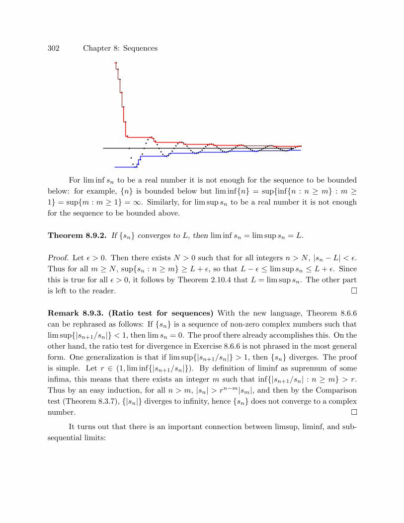
302 Chapter 8: Sequences
�
�
�
�
�
�
�
�
�
�� �
�
�
�
�
�
�� � �
�
�
�
��� � �
����� �
� ������ � � �
����� � � � � �
�� � � � � �
� �� �
� � � � � � � � � � � �� �
� �� � � � � � � � � � � �
� �� � � �
For lim inf sn to be a real number it is not enough for the sequence to be bounded
below: for example, {n} is bounded below but lim inf{n} = sup{inf{n : n ≥ m} : m ≥1} = sup{m : m ≥ 1} = ∞. Similarly, for lim sup sn to be a real number it is not enough
for the sequence to be bounded above.
Theorem 8.9.2. If {sn} converges to L, then lim inf sn = lim sup sn = L.
Proof. Let ε > 0. Then there exists N > 0 such that for all integers n > N , |sn − L| < ε.
Thus for all m ≥ N , sup{sn : n ≥ m} ≥ L + ε, so that L − ε ≤ lim sup sn ≤ L + ε. Since
this is true for all ε > 0, it follows by Theorem 2.10.4 that L = lim sup sn. The other part
is left to the reader.
Remark 8.9.3. (Ratio test for sequences) With the new language, Theorem 8.6.6
can be rephrased as follows: If {sn} is a sequence of non-zero complex numbers such that
lim sup{|sn+1/sn|} < 1, then lim sn = 0. The proof there already accomplishes this. On the
other hand, the ratio test for divergence in Exercise 8.6.6 is not phrased in the most general
form. One generalization is that if lim sup{|sn+1/sn|} > 1, then {sn} diverges. The proof
is simple. Let r ∈ (1, lim inf{|sn+1/sn|}). By definition of liminf as supremum of some
infima, this means that there exists an integer m such that inf{|sn+1/sn| : n ≥ m} > r.
Thus by an easy induction, for all n > m, |sn| > rn−m|sm|, and then by the Comparison
test (Theorem 8.3.7), {|sn|} diverges to infinity, hence {sn} does not converge to a complex
number.
It turns out that there is an important connection between limsup, liminf, and sub-
sequential limits:
Section 8.9: Liminf, limsup for real-valued sequences 303
Theorem 8.9.4. Let {sn} be a bounded sequence of real numbers. Then the supremum
of the set of all subsequential limits equals lim sup sn, and the infimum of the set of all
subsequential limits equals lim inf sn.
Proof. Proof of the limsup part only: Let A = lim sup{sn}, let S be the set of all subse-
quential limits of {sn}, and let U = sup(S). Since the sequence is bounded, A and U are
real numbers.
Let ε > 0. Since A = inf{sup{sn : n ≥ m} : m ≥ 1}, there exists m0 ≥ 1 such that
sup{sn : n ≥ m0} − A < ε. Thus for all n ≥ m0, sn − A < ε. But then any subsequential
limit of {sn} is a subsequential limit of {sn}n≥m0, so that this limit must be at most A+ ε.
Thus A+ ε is an upper bound on all subsequential limits of {sn}, so that U ≤ A+ ε. Since
ε is an arbitrary positive number, by Theorem 2.10.4 this means that U ≤ A.
By definition of U , there exists a convergent subsequence {skn} such that U −lim{skn}n < ε/2. Let L = lim{skn}n. So U − L < ε/2, and there exists a positive
real number N such that for all integers n > N , |skn − L| < ε/2. Thus for all n > N ,
skn > L− ε/2 > (U − ε/2)− ε/2 = U − ε.
Thus for any integer m ≥ N , the supremum of {sn : n > m} must be at least U − ε, so
that A, the limsup of {sn} must be at least U − ε. Hence by Theorem 2.10.4 this means
that A ≤ U .
It follows that A = U .
Theorem 8.9.5. Let {sn}, {tn} be bounded sequences in R. Then lim sup sn+lim sup tn ≥lim sup(sn + tn) and lim inf sn + lim inf tn ≤ lim inf(sn + tn).
Proof. Let a = lim sup sn, b = lim sup tn, c = lim sup(sn+tn). By boundedness, a, b, c ∈ R.
Let ε > 0. Recall that a = inf{sup{sn : n ≥ m} : m ≥ 1}. Then there exists a positive
integer m such that
sup{sn : n ≥ m} − ε < a ≤ sup{sn : n ≥ m}.
In particular for all n > m, sn − ε < a. By possibly increasing m, we similarly get that
for all n > m in addition tn − ε < b. Thus for all n > m, sn + tn − 2ε < a + b. Thus
c = inf{sup{sn + tn : n ≥ m} : m ≥ 1} ≤ a + b + 2ε. Since ε is arbitrary, it follows that
c ≤ a+ b, which proves the first part. The rest is left as an exercise.

304 Chapter 8: Sequences
Theorem 8.9.6. Let {sn} and {tn} be sequences of non-negative real numbers such that
lim sn is a positive real number L. Then lim sup(sntn) = L lim sup tn and lim inf(sntn) =
L lim inf tn.
Proof. Let ε > 0. Set ε′ = min{L/2, ε}. By assumption there exists N > 0 such that for all
integers n > N , |sn − L| < ε′. Then L− ε′ < sn < L+ ε′. Thus each sn is positive, and in
fact |sn| > L/2. It follows that (L− ε′)tn ≤ sntn ≤ (L+ ε′)tn. But then since L± ε′ ≥ 0,
(L−ε′) lim sup tn = lim sup(L−ε′)tn ≤ lim sup sntn ≤ lim sup(L+ε′)tn = (L+ε′) lim sup tn.
The proof of the liminf part is similar.
Exercises for Section 8.9
8.9.1. Let {sn} and {tn} be sequences of real numbers such that lim sn is a positive real
number L. Prove that lim sup(sn+tn) = L+lim sup tn and lim inf(sn+tn) = L+lim inf tn.
8.9.2. Compute lim inf and lim sup for the following sequences. Justify your work.
i) { sinnn }.
ii) {(−1)nn!}.iii) {2−n}.iv) {1, 2, 3, 1, 2, 3, 1, 2, 3, 1, 2, 3, 1, 2, 3, 1, 2, 3, . . .}.v) {(4 + 1
n )(−1)n}.vi) The sequence of all positive prime numbers.
vii) The sequence of all multiplicative inverses of positive prime numbers.
8.9.3. Prove the following for any sequence {sn}:i) inf(−sn) = − sup(sn).
ii) lim inf(−sn) = − lim sup(sn).
8.9.4. Suppose that {sn} converges to L. Finish the proof of Theorem 8.9.2, namely prove
that lim inf sn = L.
8.9.5. For every positive integer n, let s2n−1 = 1 and s2n = 1/2n.
i) Compute lim inf sn, lim inf sn.
ii) Prove that lim sup sn+1
sn> 1.
iii) Does this contradict the ratio test as in Remark 8.9.3.
8.9.6. Find bounded real-valued sequences {sn}, {tn} such that lim sup sn + lim sup tn >
lim sup(sn + tn). (Compare with Theorem 8.9.5.)

Section 8.9: Liminf, limsup for real-valued sequences 305
8.9.7. Let {sn}, {tn} be bounded sequences in R.
i) Finish the proof of Theorem 8.9.5, namely prove that lim inf sn + lim inf tn ≤lim inf(sn + tn).
ii) Find such {sn}, {tn} so that lim inf sn + lim inf tn < lim inf(sn + tn).
8.9.8. Suppose that lim sn = ∞. Prove that the set of subsequential limits of {sn} is
empty.
8.9.9. Finish the proof of Theorem 8.9.4, namely prove that the infimum of the set of all
subsequential limits of a bounded sequence equals the liminf of the sequence.
8.9.10. Let {sn} be a sequence of positive real numbers. Prove that lim sup 1sn
= 1lim inf sn
.

Chapter 9: Infinite series and power series
In this section we will handle (some) infinite sums, and in particular functions that
arise as infinite sums of higher and higher powers of a variable x. The culmination of
the chapter and the course are the exponential and trigonometric function, with their
properties.
Warning: Finite sums are possible by the field axioms, but infinite sums need not
make any sense at all. For example,
1 + (−1) + 1 + (−1) + 1 + (−1) + 1 + (−1) + 1 + (−1) + 1 + (−1) + 1 + (−1) · · ·
may be taken to be 0 or 1 depending on which consecutive pairs are grouped together in
a sum, or it could even be taken to be 3 by taking the first three positive 1s, and then
matching each successive −1 in the sum with the next not-yet-used +1. In this way each
±1 in the expression is used exactly once, so that the sum can indeed be taken to be 3.
Similarly, we can make the limit be 4, −17, et cetera.
This should convince you in addition that in infinite sums, the order of addition
matters! For more on the order of addition, see Theorem 9.2.8 and Exercise 9.2.16.
Infinite sums require special handling, but limits of sequences prepared the ground
for that.
9.1 Infinite series
Definition 9.1.1. For an infinite sequence {an} of complex numbers, define the corre-
sponding sequence of partial sums
{a1, a1 + a2, a1 + a2 + a3, a1 + a2 + a3 + a4, . . .}.
We denote the nth term of this sequence sn =∑nk=1 ak. The (infinite) series corre-
sponding to the sequence {an} is∑∞k=1 ak (whether this “infinite sum” makes sense or
not).
When the range of indices is clear, we write simply∑k ak or
∑ak.
Section 9.1: Infinite series 307
Example 9.1.2. For the sequence {1}, the sequence of partial sums is {n}. If a 6= 1, by
Example 1.5.4 the sequence of partial sums of {an} is {∑nk=1 a
k}n = {an+1−aa−1 }n. In par-
ticular, the sequence of partial sums of {(−1)n} is {{ (−1)n−12 }n = {−1, 0,−1, 0,−1, 0, . . .}.
We have encountered shifted sequences, such as {an}n≥m, and similarly there are
shifted series:∑∞k=m ak stands for the limit of the sequence of partials sums, but in this
case, the nth partial sum is sn = am + am+1 + am+2 + · · ·+ am+n−1.
Definition 9.1.3. (Most of the time and by default we take m = 1.) The series∑∞k=m ak
converges to L ∈ C if the sequence {∑n−m+1k=m ak}n converges to L. We say then that L
is the sum of the series and we write∑∞k=m ak = L.
If the series does not converge, it diverges.
Just like for sequences, when a series diverges, it may diverge to ∞ or to −∞, or it
may simply have no limit.
Since a sequence {sn} converges if and only if {sn + c} converges (where c is any
constant), it follows that∑∞k=1 ak converges if and only if
∑∞k=m ak converges, and then
∞∑k=1
ak = a1 + a2 + · · ·+ am−1 +∞∑k=m
ak.
The following follows immediately from the corresponding results for sequences:
Theorem 9.1.4. Let A =∑∞k=1 ak, B =
∑∞k=1 bk, and c ∈ C.
(1) If A,B ∈ C, then∞∑k=1
(ak + cbk) = A+ cB.
(2) If all ak, bk are real numbers and A,B ∈ R ∪ {∞,−∞}, then
∞∑k=1
(ak + cbk) =
∞, if A =∞, B ∈ R ∪ {∞} and c ≥ 0;∞, if A =∞, B ∈ R ∪ {−∞} and c ≤ 0;−∞, if A = −∞, B ∈ R ∪ {−∞} and c ≥ 0;−∞, if A = −∞, B ∈ R ∪ {∞} and c ≤ 0;∞, if A ∈ R, B =∞ and c > 0;−∞, if A ∈ R, B =∞ and c < 0;∞, if A ∈ R, B = −∞ and c < 0;−∞, if A ∈ R, B = −∞ and c > 0;A, if c = 0.
Proof. (1) By assumption, the sequences {∑nk=1 ak} and {
∑nk=1 bk} converge to A and B
in C, respectively. By the theorem on the convergence of sums of sequences (Theorem 8.4.3)
then∑nk=1(ak + cbk) =
∑nk=1 ak + c
∑nk=1 bk converges to A+ cB.
Other parts are proved similarly.
308 Chapter 9: Infinite series and power series
Remark 9.1.5. This theorem justifies the binary operation of addition on the set of of
convergent infinite series: ( ∞∑k=1
ak
)+
( ∞∑k=1
bk
)=∞∑k=1
(ak + bk).
It is hard to immediately present examples of this because we know so few limits of
infinite series. There are examples in the exercises.
Theorem 9.1.6. If r ∈ C satisfies |r| < 1, then the geometric series∑∞k=1 r
k−1
converges to 11−r , so
∑∞k=1 r
k = r1−r .
Proof. By Example 1.5.4,∑nk=1 r
k−1 = 1−rn1−r . By Theorem 8.6.5, lim rn = 0. Thus by the
scalar and sum rules for limits of sequences (Theorem 8.5.6 or Theorem 8.4.3),
limn→∞
n∑k=1
rk−1 = limn→∞
1− rn
1− r= limn→∞
(1
1− r− rn
1− r
)=
1
1− r.
Thus limn→∞∑nk=1 r
k = r limn→∞∑nk=1 r
k−1 = r1−r .
In particular, the familiar decimal expansion 0.33333 · · · of 1/3 can be thought of as
the infinite sum∑∞k=1
310k
. The sequence of its partial sums is {0.3, 0.33, 0.333, 0.3333, . . .},and by the theorem above,
∞∑k=1
3
10k=
3
10
∞∑k=1
(1
10
)k−1
=3
10· 1
1− 110
=3
10· 10
9=
1
3.
A little more work is expressing 5.523 = 5.523523523523 · · · (repeating 523) as a fraction:
5.523 = 5 +523
1000+
523
10002+
523
10003+ · · · = 5 + 523
∞∑k=1
(1
1000k
)
= 5 + 5231
1000
1− 11000
= 5 + 5231
1000− 1= 5 +
523
999=
4995 + 523
999
=5518
999.
Example 9.1.7. The harmonic series∑∞k=1
1k diverges to ∞ by Example 8.7.6.
Example 9.1.8.∑∞k=1
1k·(k+1) = 1.
Proof. By Exercise 8.2.9,∑nk=1
1k(k+1) = 1− 1
n+1 . Thus
∞∑k=1
1
k(k + 1)= limn→∞
n∑k=1
1
k(k + 1)= limn→∞
(1− 1
n+ 1
)= 1.

Section 9.1: Infinite series 309
Example 9.1.9. The series∑∞k=1
1k2 converges.
Proof #1: By Exercise 1.5.20 and Theorem 9.1.6,
0 ≤2n−1∑k=1
1
k2≤n+1∑k=1
1
2k−1≤∞∑k=1
1
2k−1=
1
1− 1/2= 2,
so that {∑2n−1k=1
1k2 }n and {
∑nk=1
1k2 }n are bounded increasing sequences of real numbers.
By Theorem 8.6.4, the sequence has a limit that is at most 2, so that∑∞k=1
1k2 converges.
Proof #2: Since k2 > k(k − 1), we have that for k > 2, 1k2 <
1k(k−1) . Thus
∑nk=1
1k2 =
1+∑nk=2
1k2 < 1+
∑nk=2
1k(k−1) . By Example 9.1.8, the series
∑∞k=2
1k(k−1) =
∑∞k=1
1k(k+1)
converges, so that the increasing sequence {∑nk=1
1k2 } of partial sums is bounded above, so
that by Theorem 8.6.4,∑∞k=1
1k2 converges.
It turns out that∑∞k=1
1k2 = π2
6 , but this is much harder to prove. (An indication of
the proof is in Exercise 9.12.5.)
Theorem 9.1.10. If∑∞k=1 ak converges, then lim an = 0, and the sequence {an} is
bounded.
Proof. By assumption,∑∞k=1 ak converges, so that by definition, the sequence {sn} of
partial sums converges, and is thus Cauchy. In particular, for every ε > 0 there exists
N > 0 such that for all integers n > N + 1, |an| = |sn − sn−1| < ε. Thus lim an = 0, and
by Theorem 8.6.2, {an} is bounded.
The converse of this theorem is of course false; see Example 9.1.7.
Theorem 9.1.11. Let {an} be a sequence of non-negative real numbers. If the sequence
{a1 + a2 + · · ·+ an} of partial sums is bounded above, then∑an converges.
Proof. The sequence {a1 + a2 + · · ·+ an} of partial sums is monotone and bounded above,
so it converges by Theorem 8.6.4.
Theorem 9.1.12. Let {an} be a sequence of complex numbers, and let m be a positive
integer. Then∑∞k=1 an converges if and only if
∑∞k=m an converges. Furthermore in this
case,∑∞k=1 an = (a1 + a2 + · · ·+ am−1) +
∑∞k=m an.
Proof. Let sn = a1 + a2 + · · · + an, and tn = am + am+1 + · · · + an. By the constant
and sum rules for sequences (Theorem 8.5.6 or Theorem 8.4.3), the sequence {sn}n =
{a1 + a2 + · · · + am−1}n + {tn}n converges if the sequence {tn} converges, and similarly,
{tn}n = {sn}n − {a1 + a2 + · · ·+ am−1}n converges if {sn} converges.
310 Chapter 9: Infinite series and power series
Exercises for Section 9.1
9.1.1. Let r ∈ C satisfy |r| ≥ 1. Prove that∑∞k=1 r
k diverges.
9.1.2. Compute and justify the following sums:∑∞k=1
12k
,∑∞k=6
13k
,∑∞k=8
25k
.
9.1.3. Prove that∑∞k=1
2k+1k2·(k+1)2 converges, and find the sum. (Hint: Do some initial
experimentation with partial sums, find a pattern for partial sums, and prove the pattern
with mathematical induction.)
9.1.4. Let an = (−1)n. Prove that the sequence of partial sums {a1 + a2 + · · · + an} is
bounded but does not converge. How does this not contradict Theorem 9.1.11?
9.1.5. For each k ∈ N+ let xk be an integer between 0 and 9.
i) Prove that∑∞k=1
xk10k
converges.
ii) What does this say about decimals?
iii) Find the sum if xk = 4 for all k. Express the sum with its decimal expansion and
also as a ratio of two positive integers.
iv) Find the sum if {xn} = {1, 2, 3, 1, 2, 3, 1, 2, 3, 1, 2, 3, . . .}. Express the sum with its
decimal expansion and also as a ratio of two positive integers.
(v)* Prove that whenever the sequence {xn} is eventually periodic, then∑∞k=1
xk10k
is a
rational number.
9.1.6. Prove that∑∞k=1 ak converges if and only if
∑∞k=1 Re ak and
∑∞k=1 Im ak converge.
Furthermore,∑∞k=1 ak =
∑∞k=1 Re ak + i
∑∞k=1 Im ak.
9.1.7. Suppose that lim an 6= 0. Prove that∑∞k=1 ak diverges.
9.1.8. Determine with proof which series converge.
i)∑∞k=1
1kk
.
ii)∑∞k=1
(1k3 + ik
).
iii)∑∞k=1
1k! .
9.1.9. Let {an} and {bn} be complex sequences, and let m ∈ N+ such that for all n ≥ 1,
an = bn+m. Prove that∑∞k=1 ak converges if and only if
∑∞k=1 bk converges.
9.2 Convergence and divergence theorems for series
Theorem 9.2.1. (Cauchy’s criterion for series) The infinite series∑ak converges if
and only if for all real numbers ε > 0 there exists a real number N > 0 such that for all
integers n ≥ m > N ,
|am+1 + am+2 + · · ·+ an| < ε.
Proof. Suppose that∑ak converges. This means that the sequence {sn} of partial sums
converges, and by Theorem 8.7.3 this means that {sn} is a Cauchy sequence. Thus for all
Section 9.2: Convergence and divergence theorems for series 311
ε > 0 there exists N > 0 such that for all integers m,n > N , |sn − sm| < ε. In particular
for n ≥ m > N , |am+1 + am+2 + · · ·+ an| = |sn − sm| < ε.
Now suppose that for all real numbers ε > 0 there exists a real number N > 0 such
that for all integers n ≥ m > N , |am+1 + am+2 + · · · + an| < ε. This means that the
sequence {sn} of partial sums is Cauchy. By Theorem 8.7.5, {sn} is convergent. Then by
the definition of series,∑k ak converges.
Theorem 9.2.2. (Comparison test (for series)) Let {an} be a real and {bn} a complex
sequence. such that for all n, an ≥ |bn|.(1) If
∑ak converges then
∑bk converges.
(2) If∑bk diverges then
∑ak diverges.
Proof. Note that all an are non-negative, and for all integers n ≥ m,
|bm+1 + bm+2 + · · ·+ bn| ≤ |bm+1|+ |bm+2|+ · · ·+ |bn|≤ am+1 + am+2 + · · ·+ an
= |am+1 + am+2 + · · ·+ an|.
If∑ak converges, by Theorem 9.2.1, for every ε > 0 there exists N > 0 such that for all
integers n > m > N , |am+1 +am+2 + · · ·+an| < ε, and hence |bm+1 + bm+2 + · · ·+ bn| < ε.
Thus again by Theorem 9.2.1,∑bk converges. This proves the first part.
The second part is the converse of the first.
Theorem 9.2.3. (Ratio test) (Compare to Remark 8.9.3.) Let {an} be a sequence of
non-zero complex numbers.
(1) If lim sup∣∣∣an+1
an
∣∣∣ < 1, then∑|ak| and
∑ak converge.
(2) If lim inf∣∣∣an+1
an
∣∣∣ > 1, then∑|ak| and
∑ak diverge.
Proof. Let L = lim sup |an+1
an|. Suppose that L < 1. Let r be a real number in the
open interval (L, 1). Since L = inf{sup{ |an+1||an| : n ≥ m} : m ≥ 1} and r > L, it fol-
lows that there exists m ≥ 1 such that r > sup{ |an+1||an| : n ≥ m}. Thus for all n ≥ m,
|an+1| < r|an|. Thus by Exercise 1.5.22, |am+n| < rn|am|. The geometric series∑k r
k
converges by Theorem 9.1.6, and by Theorem 9.1.4,∑k amr
k converges. Thus by Theo-
rem 9.2.2,∑∞k=1 |am+k| and
∑∞k=1 am+k converge. Hence by Theorem 9.1.12,
∑|ak| and∑
ak converge. This proves (1).
Now let L = lim inf |an+1
an|, and suppose that L > 1. Let r be a real number in the
open interval (1, L). Since L = sup{inf{ |an+1||an| : n ≥ m} : m ≥ 1} and r < L, it follows that
there exists m ≥ 1 such that r < inf{ |an+1||an| : n ≥ m}. Thus for all n ≥ m, |an+1| > r|an|.
Thus by a straightforward modification of Exercise 1.5.22, |am+n| > rn|am|. The geometric
312 Chapter 9: Infinite series and power series
series∑k r
k diverges by Exercise 9.1.1, and by Theorem 9.1.4,∑k amr
k diverges. Thus by
Theorem 9.2.2,∑∞k=1 |am+k| and
∑∞k=1 am+k diverge. Hence by Theorem 9.1.12,
∑|ak|
and∑ak diverge. This proves (2).
This ratio test for convergence of series does not apply when lim sup |an+1
an| = 1 or
lim inf |an+1
an| = 1. The reason is that under these assumptions the series
∑k |ak| and∑
k ak sometimes converge and sometimes diverge. For example, if an = 1/n for all n,
lim sup |an+1
an| = lim inf |an+1
an| = 1, and
∑nk=1
1k diverges; whereas if an = 1/n2 for all n,
then lim sup |an+1
an| = lim inf |an+1
an| = 1, and
∑nk=1
1k2 converges.
Theorem 9.2.4. (Root test for series) Let {an} be a sequence of complex numbers.
Let L = lim sup |an|1/n.
(1) If L < 1, then∑k |ak|,
∑k ak converge.
(2) If L > 1, then∑k |ak|,
∑k ak diverge.
Proof. If L < 1, choose r ∈ (L, 1). Since L = inf{sup{|an|1/n : n ≥ m} : m ≥ 1} and r > L,
there exists m ≥ 1 such that r > sup{|an|1/n : n ≥ m}. Thus for all n ≥ m, rn ≥ |an|.Thus by the Comparison test (Theorem 9.2.2), since the geometric series
∑rk converges,
we have that∑ak and
∑|ak| converge. The proof of (2) is similar, and is omitted here.
Theorem 9.2.5. (Alternating series test) If {an} is a non-increasing sequence of pos-
itive real numbers such that lim an = 0. Then∑∞k=1(−1)kak converges.
Proof. Let m,n be positive integers. Then
0 ≤ (an − an+1) + (an+2 − an+3) + · · ·+ (an+2m − an+2m+1)
= an − an+1 + an+2 − an+3 + · · ·+ an+2m − an+2m+1
= an − (an+1 − an+2)− (an+3)− an+4)− · · · − (an+2m−1 − an+2m)− an+2m+1
≤ an,
and similarly
0 ≤ an − an+1 + an+2 − an+3 + · · ·+ an+2m ≤ an.
Thus by Cauchy’s criterion Theorem 9.2.1,∑k(−1)kak converges.

Section 9.2: Convergence and divergence theorems for series 313
Example 9.2.6. Recall from Example 9.1.7 that the harmonic series∑k 1/k diverges.
But the alternating series∑k(−1)k/k converges by this theorem. (In fact,
∑k(−1)k/k
converges to − ln 2, but proving the limit is harder – see the proof after Example 9.7.5.
We examine this infinite series more carefully:
−1 +1
2− 1
3+
1
4− 1
5+
1
6− 1
7+
1
8− 1
9+
1
10− · · ·
We cannot rearrange the terms in this series as(
12 + 1
4 + 16 + 1
8 + 110 + · · ·
)minus(
1 + 13 + 1
5 + 17 + 1
9 + · · ·)
because both of these series diverge to infinity. More on
changing the order of summation is in Exercise 9.2.16 and in Theorem 9.2.8.
Definition 9.2.7. A series∑∞k=1 ak is called absolutely convergent if
∑∞k=1 |ak| con-
verges.
Theorem 9.2.8. Let∑∞k=1 ak be absolutely convergent. Let r : N+ → N+ be a bijective
function. Then∑∞k=1 ar(k) converges.
Proof. By comparison test (Theorem 9.2.2),∑∞k=1 ak converges to some number L ∈ C.
We will prove that∑∞k=1 ar(k) converges to L.
Let ε > 0. Since∑∞k=1 ak = L, there exists N0 > 0 such that for all integers
n > N0, |∑nk=1 ak − L| < ε/2. Also, since
∑∞k=1 |ak| converges, by Cauchy’s criterion for
sequences, there exists N1 > 0 such that for all integers n ≥ m > N1,∑nk=m+1 |ak| <
ε/2. Pick an integer N > max{N0, N1}. Since r is invertible, we can define M =
max{r−1(1), r−1(2), . . . , r−1(N)}. Let n be an integer strictly bigger than M . Then
by definition the set {r(1), r(2), . . . , r(n)} contains 1, 2, . . . , N . Let K = {r(k) : k ≤n} \ {1, 2, . . . , N}. Then∣∣∣∣∣
n∑k=1
ar(k) − L
∣∣∣∣∣ =
∣∣∣∣∣N∑k=1
ak +∑k∈K
ak − L
∣∣∣∣∣ ≤∣∣∣∣∣N∑k=1
ak − L
∣∣∣∣∣+∑k∈K
|ak| < ε
since all the finitely many indices in K are strictly bigger than N0.
Theorem 9.2.9. (Integral test for series convergence) Let f : [1,∞) → [0,∞) be a
decreasing function. Suppose that for all n ∈ N+,∫ n
1f exists. Then
∑∞k=1 f(k) converges
if and only if limn→∞∫ n
1f exists and is a real number.
(It is not necessarily the case that∑∞k=1 f(k) equals limn→∞
∫ n1f .)
Proof. Since f is decreasing, for all x ∈ [n, n+ 1], f(n) ≥ f(x) ≥ f(n+ 1). Thus
f(n+ 1) =
∫ n+1
n
f(n+ 1)dx ≤∫ n+1
n
f(x)dx ≤∫ n+1
n
f(n)dx = f(n).
Suppose that∑k f(k) converges. Then by the definition limn→∞(f(1) + f(2) +
· · · + f(n)) exists. By the displayed inequalities,∫ n+1
1f =
∫ 2
1f +
∫ 3
2f + · · · +
∫ n+1
nf ≤
314 Chapter 9: Infinite series and power series
f(1)+f(2)+· · ·+f(n), so that {∫ n+1
1f}n is a bounded increasing sequence of real numbers,
so that limn→∞∫ n+1
1f exists, and hence that limn→∞
∫ n1f exists.
Conversely, suppose that limn→∞∫ n
1f exists. Let L ∈ R be this limit. By the
displayed inequalities, f(2) + f(3) + · · ·+ f(n+ 1) ≤∫ 3
2f + · · ·+
∫ n+1
nf =
∫ n+1
2f . Since
f takes on only non-negative values, this says that f(2) + f(3) + · · ·+ f(n+ 1) ≤ L. Thus
{f(2) + · · · + f(n + 1)}n is a non-decreasing sequence that is bounded above by L. Thus
by Theorem 8.6.4, this sequence converges. By adding the constant f(1), the sequence
{f(1) + · · ·+ f(n+ 1)}n converges, so that by the definition of series,∑k f(k) converges.
Theorem 9.2.10. (The p-series convergence test) Let p be a real number. The series∑k k
p converges if p < −1 and diverges if p ≥ −1.
Proof. If p = −1, then the series is the harmonic series and hence diverges. If p ≥ −1,
then np ≥ n−1 for all n by Theorem 7.6.5. Thus by the comparison test (Theorem 9.2.2),∑k k
p diverges.
Now suppose that p < −1. The function f : [1,∞) → R given by f(x) = xp is
differentiable, continuous, and decreasing. Since f is continuous, for all positive integers n,∫ n1f exists. By the Fundamental theorem of calculus,
∫ n1f =
∫ n1xp dx = np+1−1
p+1 . By the
composite rule for sequences (either Theorem 8.5.8 or Theorem 8.4.7), since the function
that exponentiates by the positive −(p+1) is continuous at all real numbers and lim 1n = 0,
it follows that limnp+1 = lim(
1n
)−(p+1)= 0−(p+1) = 0, so that lim
∫ n1f exists and equals
−1p+1 . Thus by the Integral test (Theorem 9.2.9),
∑k k
p converges.
Exercises for Section 9.2
9.2.1. Prove that∑∞k=0
1(2k+1)2 ,
∑∞k=0
(−1)k
(2k+1)2 ,∑∞k=1
1k2 and
∑∞k=1
(−1)k
k2 all converge.
9.2.2. Prove that the following statements are equivalent. (They are also all true, but we
do not yet have enough methods to prove them.)
(1)∑∞k=0
1(2k+1)2 = π2
8 .
(2)∑∞k=1
1k2 = π2
6 .
(3)∑∞k=0
(−1)k
(2k+1)2 = π2
16 .
(4)∑∞k=1
(−1)k
k2 = π2
12 .
(Hint for a part: Write out the first few summands of∑∞k=1
(−1)k
k2 + 12
∑∞k=1
1k2
=∑∞k=1
(−1)k
k2 + 2∑∞k=1
1(2k)2 .)

Section 9.2: Convergence and divergence theorems for series 315
9.2.3. For each of the following series, determine with proof whether they converge or
diverge. You may need to use Examples 8.2.9 and 8.3.6.
i)
∞∑k=1
3i√k2 + k4
.
ii)
∞∑k=1
1√k
.
iii)
∞∑k=1
1
k3.
iv)∞∑k=1
2k
k!.
v)∞∑k=1
2k
k3.
vi)∞∑k=1
1
k√
2.
9.2.4. Find a convergent series∑k ak and a divergent series
∑k bk with lim sup |an|1/n =
lim sup |bn|1/n = 1.
9.2.5. Make a list of all encountered criteria of convergence for series.
9.2.6. The goal of this exercise is to show that if the ratio test (Theorem 9.2.3) determines
the convergence/divergence of a series, then the root test (Theorem 9.2.4) determines it as
well. Let {an} be a sequence of non-zero complex numbers.
i) Suppose that lim sup |an+1
an| < 1. Prove that lim sup |an|1/n < 1.
ii) Suppose that lim inf |an+1
an| > 1. Prove that lim sup |an|1/n > 1.
9.2.7. Apply the ratio test (Theorem 9.2.3) and the root test (Theorem 9.2.4) to∑∞k=1
5k
k! .
Was one test easier? Repeat for∑∞k=1
1kk
.
9.2.8. Let {an} be a complex sequence, and let c ∈ C. Is it true that∑∞k=1 ak converges
if and only if∑∞k=1 cak converges? If true, prove; if false, give a counterexample.
9.2.9. Let an = (−1)n/n, bn = 2(−1)n. Prove that∑∞k=1 ak converges, that for all n,
|bn| = 2, and that∑∞k=1
akbk
diverges.
9.2.10. (Compare with Exercise 9.2.9.) Suppose that∑∞k=1 |ak| converges. Let {bn} be a
sequence of complex numbers such that for all n, |bn| > 1. Prove that∑∞k=1
akbk
converges.

316 Chapter 9: Infinite series and power series
9.2.11. (Summation by parts) Let {an}, {bn} be complex sequences. Prove that
n∑k=1
akbk = an
n∑k=1
bk −n∑k=1
(ak+1 − ak)k∑j=1
bj .
(Hint: Set a0 = b0 = 0. Let f, g : [1,∞)→ C be defined as follows: for each n ∈ N+, on the
interval [n, n+1), f is the the constant function an−an−1 and g is the constant function bn.
Both f and g are piecewise continuous, F (n) =∫ n+1
1f = an, G(n) =
∫ n+1
1g =
∑nk=1 bk.
The problem should remind you of integration by parts∫
(Fg) = FG−∫
(fG).)
9.2.12. Let x ∈ C with |x| = 1 and x 6= 1. Prove that∑∞k=1
xk
k converges. (Hint:
Exercise 9.2.11, Example 1.5.4.)
9.2.13. Prove that if∑∞k=1 ak converges then
∑∞k=1
akk converges. (Hint: Exercise 9.2.11.)
9.2.14. (The Dirichlet test) Let {an} be a decreasing real sequnce such that lim an = 0,
and let {bn} be a sequence of complex numbers whose sequence of partial sums is bounded.
i) Prove that the series∑∞k=1 akbk converges. (Hint: Exercise 9.2.11.)
ii) Prove the alternating series test using part i).
9.2.15. The following guides through another proof of the p-series convergence test for
p < −1. (Confer Theorem 9.2.10 for the first proof).
i) Prove that for each positive integer n there exists c ∈ (n, n+1) such that (p+1)cp =
(n+ 1)p+1 − np+1. (Hint: Mean value theorem (Theorem 6.3.4).)
ii) Prove that for all positive integers n,
(n+ 1)p <(n+ 1)p+1 − np+1
p+ 1and np <
np+1 − (n− 1)p+1
p+ 1.
iii) Prove by induction on n ≥ 1 that
n∑k=1
kp ≤ 1
p+ 1np+1 +
p
p+ 1.
iv) Prove that the positive sequence {∑nk=1 k
p}n of partial sums is an increasing se-
quence bounded above.
v) Prove that the sequence {∑nk=1 k
p}n converges, and so that∑∞k=1 k
p converges.
9.2.16. (Order of summation in infinite sums is important.)
i) Prove that∑∞k=1
12k and
∑∞k=1
12k+1 diverge. Refer to Example 9.2.6.
ii) Observe that∑nk=1
12k −
∑nk=1
12k+1 =
∑2n+1k=1
(−1)k
k .
iii) Argue that∑∞k=1
(−1)k
k 6=∑∞k=1
12k −
∑∞k=1
12k+1 . Why does this not contradict
the “expected” summation and difference rules?

Section 9.3: Power series 317
9.2.17. (Raabe’s test) Let a1, a2, . . . be positive real numbers such that for some α > 1
and for some N ∈ N, an+1
an≤ 1 − α
n for all n ≥ N . Prove that∑n an converges. (Hint:
Let f(x) = 1− xα. Use the Mean value theorem to get c ∈ (x, 1) such that f ′(c)(1− x) =
f(1)− f(x). Conclude that 1− xα ≤ (1− x)α. Apply this to x = 1− 1n . Use that
∑n−α
converges.)
9.3 Power series
In this section we deal with sums where the index varies through N0, and furthermore,
the terms of the sequence are special functions rather than constants:
Definition 9.3.1. A power series is an infinite series of the form
∞∑k=0
akxk =
∑k≥0
akxk = a0 + a1x+ a2x
2 + a3x3 + · · · ,
where a0, a1, a2, . . . are fixed complex numbers, and x is a variable that can be replaced by
any complex number. (By convention as on page 35, 00 = 1.)
Think through the following table of reading off the coefficients an of xn:
power series an∞∑k=0
xk an = 1
∞∑k=0
x2k+1 = x+ x3 + x5 + x7 + · · · an =
{1, if n is odd;0, if n is even.
∞∑k=0
x2k+12 = x12 + x14 + x16 + x18 + · · · an =
{0, if n is odd;0, if n is even and n < 12;1, if n ≥ 12 is even.
∞∑k=0
kxk an = n
∞∑k=0
xk
k!an = 1
n!
∞∑k=0
(kx)k an = nn
The partial sums of power series are polynomials, so a power series is a limit of
polynomials.

318 Chapter 9: Infinite series and power series
A power series is a function of x, and the domain is to be determined. Clearly, 0
is in the domain of every power series: plugging in x = 0 returns∑∞k=0 ak0k = a0. If all
except finitely many an are 0, then the power series is actually a polynomial, and is thus
defined on all of C. When 1 is in the domain, evaluation of the power series∑k akx
k at
x = 1 is the (ordinary) series∑k ak.
The most important question that we address in this section is: which x are in the
domain of the power series, i.e., for which x does such an infinite series converge. We prove
that for every power series whose domain is not all of C there exists a non-negative real
number R such that the series converges for all x ∈ C with |x| < R and the series diverges
for all x ∈ C with |x| > R. What happens at x with |x| = R depends on the series.
Example 9.3.2. Let f(x) =∑∞k=0 x
k. By Theorem 9.1.6, the domain of f contains all
complex numbers with absolute value strictly smaller than 1, and by Theorem 9.1.10, the
domain of f contains no other numbers, so that the domain equals {x ∈ C : |x| < 1}.Moreover, for all x in the domain of f , by Theorem 9.1.6,
∑∞k=0 x
k = 11−x . Note that the
domain of 11−x is strictly larger than the domain of f .
Whereas for general power series it is impossible to get a true numerical infinite sum,
for geometric series this is easy: f( 12 ) =
∑k≥0
12k
= 11− 1
2
= 2, f( 13 ) =
∑k≥0
13k
= 11− 1
3
= 32 ,
f(0.6) =∑k≥0 0.6k = 1
1−0.6 = 2.5.
Theorem 9.3.3. (Root test for the convergence of power series) Let∑akx
k be a
power series, and let α = lim sup |an|1/n. Define R by
R =
1/α, if 0 < α <∞;0, if α =∞;∞, if α = 0.
Then for all x ∈ C with |x| < R,∑|ak||x|k and
∑akx
k converge in C, and for all x ∈ Cwith |x| > R,
∑|ak||x|k and
∑akx
k diverge.
Proof. By the definition of limits, α is either a non-negative real number or ∞. We apply
the Root test for series (Theorem 9.2.4): lim sup |anxn|1/n = |x| lim sup |an|1/n = |x|α. If
|x|α < 1, then both of the series converge, and if |x|α > 1, then the two series diverge. If
α = 0, then |x|α < 1 is true for all x ∈ C, so R = ∞ has the stated property. If α = ∞,
then |x|α < 1 is true only for x = 0, so R = 0 has the stated property. If 0 < α <∞, then
|x|α < 1 is true only for all x ∈ C with |x| < 1/α = R.

Section 9.3: Power series 319
Definition 9.3.4. The R from Theorem 9.3.3 is called the radius of convergence of
the series∑akx
k.
This is really a radius of convergence because inside the circle B(0, R) the series
converges and outside of the circle the series diverges. Whether the power series converges
at points on the circle depends on the series; see Example 9.3.6.
Theorem 9.3.5. The series∑akx
k,∑|ak|xk,
∑|ak||x|k,
∑kak|x|k,
∑kakx
k−1,∑k2akx
k,∑k(k − 1)akx
k, all have the same radius of convergence.
Proof. By Example 8.2.9, lim n√|n| = 1. For any integer n ≥ 2, 1 ≤ n
√n− 1 ≤ n
√n, so that
by the squeeze theorem, lim n√n− 1 = 1. Thus by Theorem 8.9.6, lim sup n
√|n(n− 1)an| =
lim n√n(n− 1) · lim sup n
√|an| = lim sup n
√|an|. This proves that the α as in Theorem 9.3.3
for∑akx
k is the same as the α for∑k(k − 1)akx
k, which proves that these two power
series have the same radius of convergence. The proofs of the other parts are similar.
Example 9.3.6. We have seen that∑xk has radius of convergence 1. By Theorem 9.1.10,
this series does not converge at any point on the unit circle. By the previous theorem,
the radius of convergence of∑∞k=1
1kx
k and of∑∞k=1
1k2x
k is also 1. By the p-series test
(Theorem 9.2.10) or by the harmonic series fact,∑∞k=1
1kx
k diverges at x = 1, and by the
alternating series test (Theorem 9.2.5),∑∞k=1
1kx
k converges at x = −1. By the p-series
test (Theorem 9.2.10),∑∞k=1
1k2 converges, so that by the comparison test Theorem 9.2.2,∑∞
k=11k2x
k converges on the unit circle.
Theorem 9.3.7. Let the radius of convergence for∑akx
k be R. Then the radius of
convergence for∑akx
2k is ∞ if R =∞ and it is√R otherwise.
Proof. Let α = lim sup n√|an|. In the second power series, the nth coefficient is 0 if n is
odd, and it is an/2xn if n is even. Then applying the root test to this power series gives
lim sup{
1√
0, 2√|a1|, 3
√0, 4√|a2|, 5
√0, 6√|a3|, 7
√0, 8√|a4|, . . .
}= lim sup
{2√|a1|, 4
√|a2|, 6
√|a3|, 8
√|a4|, . . .
}(0s do not contribute to limsup of non-negative numbers)
= lim sup
{√1√|a1|,
√2√|a2|,
√3√|a3|,
√4√|a4|, . . .
}=
√lim sup
{1√|a1|, 2
√|a2|, 3
√|a3|, 4
√|a4|, . . .
}=√α,
and the conclusion follows.
320 Chapter 9: Infinite series and power series
Example 9.3.8. Similarly to the last example and by Theorem 9.3.5,∑xk,
∑kxk,∑
k2xk,∑k(k − 1)xk,
∑x2k+1 all have radius of convergence 1.
Theorem 9.3.9. (Ratio test for the convergence of power series) Suppose that all
an are non-zero complex numbers.
(1) If |x| < lim inf∣∣ anan+1
∣∣, then∑|ak||x|k and
∑akx
k converge.
(2) If |x| > lim sup∣∣ anan+1
∣∣, then∑|ak||x|k and
∑akx
k diverge.
Thus if lim∣∣ anan+1
∣∣ exists, it equals the radius of convergence of∑akx
k.
Warning: Compare with the Ratio test for convergence of series (Theorem 9.2.3)
where fractions are different. Explain to yourself why that is necessarily so, possibly after
going through the proof below.
Proof. The two series converge in case x = 0, so that we may assume that x 6= 0. We may
then apply the Ratio test for convergence of series (Theorem 9.2.3):
lim sup
∣∣∣∣an+1xn+1
anxn
∣∣∣∣ = |x| lim sup
∣∣∣∣an+1
an
∣∣∣∣= |x| inf{sup
{∣∣∣∣an+1
an
∣∣∣∣ : n ≥ m}
: m ≥ 1}
= |x| inf
{1
inf{∣∣ anan+1
∣∣ : n ≥ m}: m ≥ 1
}
=|x|
sup{
inf{∣∣ anan+1
∣∣ : n ≥ m} : m ≥ 1}
=|x|
lim inf∣∣ anan+1
∣∣ .If this is strictly smaller than 1, then the two series converge, which proves (1). Similarly,
lim inf
∣∣∣∣an+1xn+1
anxn
∣∣∣∣ =|x|
lim sup∣∣ anan+1
∣∣ ,and if this is strictly larger than 1, then the two series diverge. The last part is then
immediate by the definition of radius of convergence.
Examples 9.3.10.
(1) In Example 9.3.8 we established via the root test that∑x2k+1 has radius of
convergence 1. The ratio test is inapplicable for this power series. However, note
that∑x2k+1 = x
∑(x2)k, and by the ratio test for series (not power series), this
series converges for non-zero x if lim sup |(x2)k+1/(x2)k| < 1, i.e., if |x2| < 1, i.e.,
if |x| < 1, and it diverges if |x| > 1.
Section 9.3: Power series 321
(2) The radius of convergence of∑∞k=1
(xk
)kis ∞. For this we apply the root test:
α = lim sup∣∣ 1nn
∣∣1/n = lim sup 1n = 0.
(3) By the ratio test, the radius of convergence of∑∞k=1
xk
k! is lim∣∣ 1
n!1
(n+1)!
∣∣ = lim (n+1)!n! =
lim(n+1) =∞. The root test gives α = lim sup |1/n!|1/n| = lim sup(1/n!)1/n, and
by Example 8.3.6 this is 0. Thus the radius of convergence is ∞ also by the root
test.
Exercises for Section 9.3
9.3.1. Let the radius of convergence of∑∞k=0 akx
k be R. Let c ∈ C.
i) Prove that c ·∑∞k=0 akx
k =∑∞k=0(c ·ak)xk is convergent with radius of convergence
equal to R if c 6= 0, and with radius of convergence ∞ otherwise.
ii) Prove that∑∞k=0 ak(cx)k is convergent with radius of convergence equal to ∞ if
c = 0 and radius R/|c| otherwise.
9.3.2. Suppose that∑k ak converges for some ak ∈ C.
i) Prove that the function defined as the power series∑k akx
k has radius of conver-
gence at least 1.
ii) Give an example of ak ∈ C for which the radius of convergence of∑∞k=0 akx
k is
strictly greater than 1. (Bonus points for easiest example.)
iii) Give an example of ak ∈ C for which the radius of convergence of∑∞k=0 akx
k is
equal to 1.
9.3.3. Compare with the previous exercise: find the radii of convergence of the power series∑∞k=0 x
k,∑∞k=0(−1)xk,
∑∞k=0(2x)k,
∑∞k=0 x
k +∑∞k=0(−1)xk,
∑∞k=0 x
k +∑∞k=0(2x)k.
9.3.4. Compute and justify the radius of convergence for the following series:
i)∑
3xk.
ii)∑
(3x)k.
iii)∑
3kxk.
iv)∑k(3x)k.
v)∑
xk
k3 .
vi)∑
3xk
k3 .
vii)∑ (3x)k
k3 .
9.3.5. Compute and justify the radius of convergence for the following series:
i)∑
xk
kk.
ii)∑
xk
k2k.
iii)∑
xk
(2k)k.
322 Chapter 9: Infinite series and power series
9.3.6. Let∑∞k=0 akx
k and∑∞k=0 bkx
k be convergent power series with radii of convergence
R1 and R2, respectively. Let R = min{R1, R2}. Prove that∑∞k=0 akx
k ±∑∞k=0 bkx
k =∑∞k=0(ak±bk)xk is convergent with radius of convergence at leastR. (Hint: Theorem 9.1.4.)
9.3.7. Let R be the radius of convergence of∑∞k=0 akx
k. Let p be a positive integer.
i) Determine the radius of convergence of∑∞k=p akx
k.
ii) Determine the radius of convergence of∑∞k=0 akx
pk.
9.3.8. What would be a sensible definition for generalized power series∑∞k=0 ak(x−a)k?
What would be a sensible definition of the radius of convergence of∑∞k=0 ak(x−a)k? Draw
a relevant picture in C.
9.4 Differentiation of power series
Power series are functions. In this section we prove that they are differentiable at all
x inside the circle of convergence. Since a differentiable function is continuous, it follows
that a power series is continuous inside the circle of convergence.
Recall that for any differentiable function f , f ′(x) = limh→0f(x+h)−f(x)
h , and any
power series∑∞k=0 akx
k is actually the limit of a sequence:∑∞k=0 akx
k = lim{∑nk=0 akx
k}n.
Thus
(∞∑k=0
akxk)′ = lim
h→0
lim{∑nk=0 ak(x+ h)k}n − lim{
∑nk=0 akx
k}nh
.
Certainly by the sum rule for convergent series, lim{∑nk=0 ak(x+h)k}n−lim{
∑nk=0 akx
k}n =
lim{∑nk=0 ak((x+ h)k − xk)}n, and by the constant rule we get that
(∞∑k=0
akxk)′ = lim
h→0limn→∞
n∑k=0
ak(x+ h)k − xk
h.
If we could change the order of limits, then we would get by the polynomial rule for
derivatives that
(∞∑k=0
akxk)′ = lim
n→∞limh→0
n∑k=0
kakxk−1.
In fact, it turns out that this is the correct derivative, but our reasoning above was based
on an unproven (and generally false) switch of the two limits.
We give a correct proof of derivatives in the rest of the section. By Theorem 9.3.5
we already know that the series∑∞k=0 akx
k and∑∞k=0 kakx
k−1 =∑∞k=1 kakx
k−1 have the
same radius of convergence.
The following theorem is not necessarily interesting in its own right, but it is a
stepping stone in the proof of derivatives of power series.
Section 9.4: Differentiation of power series 323
Theorem 9.4.1. Let∑k akx
k have radius convergence R. Let c ∈ C satisfy |c| < R. Then
the function g(x) =∑∞k=1 ak(xk−1 + cxk−2 + c2xk−3 + · · · + ck−1) is defined on B(0, R)
and is continuous at c.
Proof. There is nothing to prove if R = 0, so we may assume that R > 0.
First of all,∑∞k=1 kakx
k−1 converges on B(0, R) by Theorem 9.3.5. In particular,∑∞k=1 kakc
k−1 =∑∞k=1 ak(ck−1 + cck−2 + c2ck−3 + · · · + ck−1) is well-defined, but this is
simply g(c), so that c is in the domain of g.
Let ε > 0 and let d ∈ R satisfy |c| < d < R. Then again by Theorem 9.3.5, d is in the
domain of∑k akx
k,∑k kakx
k−1, and also∑k k(k− 1)akx
k−2 and∑k k(k− 1)|ak||x|k−2.
Set D = 12
∑k k(k − 1)|ak|dk−2, and δ = min{d− |c|, ε
D+1}. Then δ is positive. Let c ∈ Cwith 0 < |x − c| < δ. Then by the triangle inequality, |x| = |x − c + c| ≤ |x − c| + |c| <δ + |c| ≤ d− |c|+ |c| = d < R, so that x is in the domain of the power series
∑k akx
k.
But is x in the domain of g? Since the radius of convergence of∑k akx
k is R, by
Theorem 9.3.5 also the radius of convergence of∑k kakx
k−1 is R, so that∑k kakd
k−1
converges. Then from the Comparison theorem (Theorem 9.2.2) and from
|ak(xk−1 + cxk−2 + c2xk−3 + · · ·+ ck−1)|≤ |ak|(|x|k−1 + |c||x|k−2 + |c|2|x|k−3 + · · ·+ |c|k−1) (by the triangle inequality)
≤ |ak|(dk−1 + ddk−2 + d2dk−3 + · · ·+ dk−1)
= k|ak|dk−1
we deduce that x is in the domain of g. Furthermore,
|g(x)− g(c)| = |∑
ak(xk−1 + cxk−2 + c2xk−3 + · · ·+ ck−1)−∑
kakck−1|
= |∑
ak(xk−1 + cxk−2 + c2xk−3 + · · ·+ ck−1 − kck−1)|
= |∑
ak((xk−1 − ck−1) + (cxk−2 − ck−1) + (c2xk−3 − ck−1) + · · ·+ (ck−1 − ck−1)|
= |∑
ak((xk−1 − ck−1) + c(xk−2 − ck−2) + c2(xk−3 − ck−3) + · · ·+ ck−2(x− c))|
= |∑
ak(x− c)((xk−2 + xk−3c+ xk−4c2 + · · ·+ ck−2)
+ c(xk−3 + xk−4c+ xk−5c2 + · · ·+ ck−3)
+ c2(xk−4 + xk−5c+ xk−6c2 + · · ·+ ck−4) + · · ·+ ck−2)| (by Exercise 1.5.21)
≤∑|ak||x− c|((|x|k−2 + |x|k−3|c|+ |x|k−4|c|2 + · · ·+ |c|k−2)
+ |c|(|x|k−3 + |x|k−4|c|+ |x|k−5|c|2 + · · ·+ |c|k−3)
+ |c|2(|x|k−4 + |x|k−5|c|+ |x|k−6|c|2 + · · ·+ |c|k−4) + · · ·+ |c|k−2)
(by the triangle inequality)
≤ |x− c|∑|ak|((dk−2 + dk−3d+ dk−4d2 + · · ·+ dk−2)

324 Chapter 9: Infinite series and power series
+ d(dk−3 + dk−4d+ dk−5d2 + · · ·+ dk−3)
+ d2(dk−4 + dk−5d+ dk−6d2 + · · ·+ dk−4) + · · ·+ dk−2)
= |x− c|∑|ak|((k − 1)dk−2 + (k − 2)dk−2 + (k − 3)dk−2 + · · ·+ dk−2)
= |x− c|∑|ak|
k(k − 1)
2dk−2 (by Example 1.5.1)
= |x− c|D< δD
< ε.
This proves that g is continuous at c.
Theorem 9.4.2. Let f(x) =∑∞k=0 akx
k have radius of convergence R. Then f is differen-
tiable on B(0, R), and for all c ∈ B(0, R), f ′(c) =∑∞k=1 kakc
k−1. The derivative function
f ′(x) =∑∞k=0 kakx
k−1 =∑∞k=1 kakx
k−1 also has radius of convergence R.
Proof. Let c, x ∈ B(0, R). Then
f(x)− f(c)
x− c=
∑k akx
k −∑k akc
k
x− c
=
∑k ak(xk − ck)
x− c
=
∑k ak(x− c)(xk−1 + xk−2c+ xk−3c2 + · · ·+ ck−1)
x− c(by Exercise 1.5.21)
=∑k
ak(xk−1 + xk−2c+ xk−3c2 + · · ·+ ck−1),
which is the function g from the previous theorem. In that theorem we proved that g is
continuous at c, so that
f ′(c) = limx→c
f(x)− f(c)
x− c= limx→c
g(x) = g(c) =
∞∑k=1
kakck−1.
Then the theorem follows from Theorem 9.3.5.
Theorem 9.4.3. Suppose that the power series∑∞k=0 akx
k has radius of convergence R
and that the power series∑∞k=0 bkx
k has radius of convergence S. Suppose that for some
positive r ≤ R,S the two power series take on the same values at all z ∈ Br(0). Then for
all n ≥ 0, an = bn.
In other words, if for all x ∈ Br(0),∑∞k=0 akx
k =∑∞k=0 bkx
k, then the two series are
identical.
Proof. Let f(x) =∑∞k=0 akx
k and g(x) =∑∞k=0 bkx
k. By assumption a0 = f(0) = g(0) =
b0. Let n ∈ N+. By Theorem 9.4.2, f and g are differentiable on Br(0), and since they
Section 9.5: Numerical evaluations of some series 325
are identical, their nth derivatives agree on Br(0) as well. By an n-fold application of the
derivative,
f (n)(x) =
∞∑k=n
akk(k − 1)(k − 2) · · · (k − n+ 1)xk−n,
and similarly for g(n). But then
ann(n− 1)(n− 2) · · · (n− n+ 1) = f (n)(0) = g(n)(0)bnn(n− 1)(n− 2) · · · (n− n+ 1),
so that an = bn.
Exercises for Section 9.4
9.4.1. Consider the function f(x) = 11−x and its corresponding geometric series on B(0, 1).
i) Compute a derivative of f as a rational function and as a power series.
ii) Compute an antiderivative of f as a rational function and as a power series.
9.4.2. Let f(x) =∑∞k=0
x2k+1
(2k+1)k! .
i) Find the radius of convergence of the series.
ii) Compute the derivative of f .
iii) By Example 9.7.3 we know that for every real x, ex =∑∞k=0
xk
k! . Find the series
for e(x2).
iv) Find a power series whose derivative is e(x2). (Comment: abc
might stand for (ab)c
or for a(bc). But the first form is simply abc, so we would not write abc
to stand for
that. So, it is standard notation to write abc
when we mean a(bc), In particular,
e(x2) can be written more plainly as ex2
.)
v) Address the no-closed-form discussion on page 246.
9.5 Numerical evaluations of some series
Differentiation of power series is a powerful tool. For all complex numbers x ∈ B(0, 1)
the geometric series∑∞k=0 x
k converges to 11−x . Certainly it is much easier to compute 1
1−xthan the infinite sum. We can exploit geometric series and derivatives of power series to
compute many other infinite sums. Below we provide a few illustrations of the method.
326 Chapter 9: Infinite series and power series
Example 9.5.1.∑∞k=1
k2k−1 = 4.
Proof. Let f(x) =∑∞k=0 x
k. This is the geometric series with radius of convergence 1 that
converges to 11−x (Example 9.3.2). By Theorem 9.4.2, f ′(x) =
∑∞k=0 kx
k−1 =∑∞k=1 kx
k−1,
and by Theorem 9.3.5, the radius of convergence of f ′ is also 1. Thus 12 is in the domain
of f ′. Since we have two ways of expressing f (as power series and as a rational function),
there is similarly also a second form for f ′:
f ′(x) =
(1
1− x
)′=
1
(1− x)2.
From the two forms we deduce that∑∞k=0
k2k−1 =
∑∞k=0 k
(12
)k−1= f ′(1/2) = 1
(1−1/2)2 = 4.
Example 9.5.2.∑∞k=0
k2
2k= 6, and
∑∞k=0
k2
2k−1 = 12.
Proof. As in the previous example we start with the geometric series f(x) =∑∞k=0 x
k
that converges on B(0, 1). Its derivative f ′(x) =∑∞k=0 kx
k−1 = 1(1−x)2 also converges
on B(0, 1). Then xf ′(x) =∑∞k=0 kx
k and its derivative (xf ′(x))′ =∑∞k=0 k
2xk−1 also
converge on B(0, 1). From
∞∑k=0
k2xk−1 = (xf ′(x))′ =
(x
(1− x)2
)′=
1 + x
(1− x)3
we deduce that∑∞k=0
k2
2k−1 =(
1+ 12
(1−1/2)3
)= 3/2
1/8 = 12, and∑∞k=0
k2
2k= 6.
Example 9.5.3. From the previous example we know that∑∞k=0 k
2xk−1 = 1+x(1−x)3 . Mul-
tiplying both sides by x gives∑∞k=0 k
2xk = x+x2
(1−x)3 , and differentiation gives
∞∑k=0
k3xk−1 =d
dx
(x+ x2
(1− x)3
)=
1 + 4x+ x2
(1− x)4.
It follows that∑∞k=0
k3
2k−1 = 1+4·0.5+0.52
(1−0.5)4 = 52 and∑∞k=0
k3
2k= 26.
Summary:∑∞k=0
12k−1 = 2,
∑∞k=0
k2k−1 = 4,
∑∞k=0
k2
2k−1 = 12,∑∞k=0
k3
2k−1 = 26. Is it
possible to predict∑∞k=0
k4
2k−1 ?
Example 9.5.4.∑∞k=1
1k2k
= ln 2.
Proof. Let f(x) =∑∞k=1
xk
k . The radius of convergence of f is 1, so 1/2 is in its domain.
Also, f ′(x) =∑∞k=1 x
k−1 = 11−x , so that f(x) = − ln(1− x) + C for some constant C. In
particular, C = −0 +C = − ln(1− 0) +C = f(0) = 0, so that∑∞k=1
1k2k
=∑∞k=1
1k
(12
)k=
f( 12 ) = − ln(1− 1
2 ) = − ln( 12 ) = ln(2).

Section 9.6: Some technical aspects of power series 327
Exercises for Section 9.5
9.5.1. Compute and justify∑∞k=1
1k3k
.
9.5.2. Consider∑∞k=1
kk+2·3k . According to my computer the partial sum of the first 1000
terms is a rational number whose numerator and denominator take several screen pages,
so this sum as a rational number is hard to comprehend. So instead I computed curtailed
decimal expansions for this and for a few other sums: according to my computer, the
partial sum of the first 10 terms is about 0.719474635555091, the partial sum of the first
100 terms is about 0.719487336054311, the partial sum of the first 1000 terms is about
0.719487336054311. What can you suspect? How would you go about proving it?
9.6 Some technical aspects of power series
This section is meant as a reference, and should probably be skipped in a first class
on power series.
The result below seems obvious, but the proof is nevertheless a bit involved.
Theorem 9.6.1. Let∑∞k=0 akx
k and∑∞k=0 bkx
k be convergent power series with radii
of convergence R1 and R2, respectively. Let R = min{R1, R2}. Then on B(0, R)
the product sequence {(∑nk=0 akx
k) · (∑nk=0 bkx
k)}n converges to the power series∑∞k=0(
∑kj=0 ajbk−j)x
k.
We write this as (∑∞k=0 akx
k) · (∑∞k=0 bkx
k) =∑∞k=0(
∑kj=0 ajbk−j)x
k on B(0, R).
Proof. If R = 0, there is nothing to prove. So we may assume that R is a positive real
number or it is ∞. Let x ∈ B(0, R).
Set L =∑∞k=0 akx
k and K =∑∞k=0 bkx
k (these limits exist as |x| < R1, R2), sn =∑nk=0 akx
k, tn =∑nk=0 bkx
k, and cn =∑nj=0 ajbn−j . By the theorem on the convergence
of products of sequences (Theorem 8.4.3), lim(sntn) = LK. Thus we need to prove that∑∞k=0 ckx
k = LK.
Let ε > 0. By convergence of products, there exists N1 > 0 such that for all integers
n > N1, |sntn − LK| < ε/2. By expanding (repeated “foiling”) and by grouping,
sntn =
(n∑k=0
akxk
) n∑j=0
bjxj
=
n∑k=0
k∑m=0
ambk−mxk +
n∑k=1
n∑m=k
ambn+k−mxn+k
=n∑k=0
ckxk +
n∑k=1
n∑m=k
ambn+k−mxn+k.

328 Chapter 9: Infinite series and power series
Since |x| < R ≤ R1, R2, the series∑∞k=0 |akxk| and
∑∞k=0 |bkxk| converge, to L, K, respec-
tively. Thus there exists N2 > 0 such that for all integers n > N2,
∞∑k=n+1
|akxk| =
∣∣∣∣∣∞∑k=0
|akxk| −n∑k=0
|akxk|
∣∣∣∣∣ < ε
4K + 1,
and similarly there exists N3 > 0 such that for all integers n > N3,∑∞k=n+1 |bkxk| <
ε
4L+1.
Now let n > max{2N1, N2, N3}. Then, with possibly adding more non-negative terms in
the third line below,
n∑k=1
n∑m=k
∣∣ambn+k−mxn+k
∣∣=
n∑k=1
bn/2c∑m=k
∣∣amxmbn+k−mxn+k−m∣∣+
n∑k=1
n∑m=max{k,bn/2c+1}
∣∣amxmbn+k−mxn+k−m∣∣
≤
bn/2c∑m=1
|amxm|
n∑k=bn/2c
∣∣bkxk∣∣+
n∑m=bn/2c
|amxm|
bn/2c∑k=1
∣∣bkxk∣∣
≤ L ε
4L+ 1+
ε
4K + 1K
<ε
2.
Thus ∣∣∣∣∣n∑k=0
ckxk − LK
∣∣∣∣∣ =
∣∣∣∣∣n∑k=0
ckxk − sntn + sntn − LK
∣∣∣∣∣≤
∣∣∣∣∣n∑k=0
ckxk − sntn
∣∣∣∣∣+ |sntn − LK|
<
∣∣∣∣∣n∑k=1
n∑m=k
ambn+k−mxn+k
∣∣∣∣∣+ ε/2
< ε/2 + ε/2 = ε.
Theorem 9.6.2. Let f(x) =∑∞k=0 ckx
k have radius of convergence a positive real num-
ber R. Let a ∈ C with |a| = R such that∑∞k=0 cka
k converges. Let B be an open ball
centered at a, and let g : B → C be continuous. If f(x) = g(x) for all x ∈ B(0, R) ∩ B,
then f(a) = g(a).
Proof. Let ε > 0. We want to show that |f(a)− g(a)| < ε, which will via Theorem 2.10.4
then prove that f(a) = g(a). It suffices to prove the inequality |f(a)− g(a)| < ε under the
additional assumption that ε < 1.
Since∑∞k=0 cka
k converges, by Cauchy’s criterion Theorem 9.2.1, there exists a posi-

Section 9.6: Some technical aspects of power series 329
tive integer N such that for all integers n ≥ N , |∑nk=N cka
k| < ε/4. Let sm =∑N+mk=N cka
k.
By assumption, for all m ≥ 1, |sm| < ε/4 < 1. Furthermore, cN = s0/aN , and for n > N ,
cN+n = (sn − sn−1)/aN+n.
Let r be a positive real number strictly smaller than 1. First we do a simple expan-
sion:
rNs0+(s1 − s0)rN+1 + (s2 − s1)rN+2 + · · ·+ (sn − sn−1)rN+n
= rNcNaN + cN+1a
N+1rN+1 + cN+2aN+2rN+2 + · · ·+ cN+na
N+nrN+n
=N+n∑k=N
ck(ra)k.
Thus by more rewriting and by the triangle inequality,∣∣∣∑N+n
k=N ck(ra)k∣∣∣ equals
=∣∣rNs0 + (s1 − s0)rN+1 + (s2 − s1)rN+2 + · · ·+ (sn − sn−1)rN+n
∣∣=∣∣s0(rN − rN+1) + s1(rN+1 − rN+2) + · · ·+ sn−1(rN+n−1 − rN+n) + snr
N+n∣∣
= rN∣∣(1− r) (s0 + s1r + · · ·+ sn−1r
n−1)
+ snrn∣∣
≤ rN((1− r)
(|s0|+ |s1|r + · · ·+ |sn−1|rn−1
)+ |sn|rn
)≤ ε
4rN((1− r)
(1 + r + · · ·+ rn−1
)+ rn
)(since |sm| < ε/4 for sufficiently large m)
=ε
4rN (1− rn + rn) (by Example 1.5.4)
=ε
4rN
<ε
4.
In particular,∣∣∑∞
k=N ck(ra)k∣∣ ≤ ε
4 .
Since polynomial functions are continuous, there exists δ1 > 0 such that for all
x ∈ B(a, δ1),∣∣∣∑N−1
k=0 ckxk −
∑N−1k=0 cka
k∣∣∣ < ε/4.
Since g is continuous at a, there exists δ2 > 0 such that for all x ∈ B(a, δ2), |g(x)−g(a)| < ε/4. Let r ∈ (0, 1) such that 1− r < 1
R min{δ1, δ2}. Then |a− ra| < δ1, δ2, so that
|g(a)− f(a)| =
∣∣∣∣∣g(a)− g(ra) + g(ra)− f(ra) + f(ra)−N−1∑k=0
ckak +
N−1∑k=0
ckak − f(a)
∣∣∣∣∣≤ |g(a)− g(ra)|+ |g(ra)− f(ra)|+
∣∣∣∣∣f(ra)−N−1∑k=0
ckak
∣∣∣∣∣+
∣∣∣∣∣N−1∑k=0
ckak − f(a)
∣∣∣∣∣= |g(a)− g(ra)|+ 0 +
∣∣∣∣∣∞∑k=N
ck(ra)k +N−1∑k=0
ck(ra)k −N−1∑k=0
ckak
∣∣∣∣∣+
∣∣∣∣∣∞∑k=N
ckak
∣∣∣∣∣
330 Chapter 9: Infinite series and power series
<ε
4+
∣∣∣∣∣∞∑k=N
ck(ra)k
∣∣∣∣∣+
∣∣∣∣∣N−1∑k=0
ck(ra)k −N−1∑k=0
ckak
∣∣∣∣∣+
∣∣∣∣∣∞∑k=N
ckak
∣∣∣∣∣<ε
4+ε
4+ε
4+ε
4= ε.
Since ε is arbitrary, by Theorem 2.10.4, f(a) = g(a).
Exercises for Section 9.6
9.6.1. Let∑∞k=0 akx
k,∑∞k=0 bkx
k be power series and R a positive real number such that
for all x ∈ B(0, R),(∑∞
k=0 akxk)·(∑∞
k=0 bkxk)
= 1. In other words, at each x in B(0, R),
the two infinite series are multiplicative inverses of each other.
i) Prove that for all x ∈ B(0, R),∑∞k=0 akx
k 6= 0.
ii) Prove that a0 6= 0.
iii) Prove that b0 = 1a0
, and that for all k > 0, bk = − 1a0
∑kj=1 ajbk−j . (Hint: Theo-
rem 9.6.1.)
iv) Suppose that there exists M ∈ R such that for all non-negative integers n,
|anxn| < M . Prove that for all integers k ≥ 1, |bkxk| ≤ M|a0|2 (M+|a0|
|a0| )k−1. (Hint:
induction.)
9.6.2. (Abel’s lemma) Suppose that a0, a1, a2, . . . are complex numbers and that∑k ak
converges. Let f(x) =∑k akx
k. The goal of this exercise is to prove that f is defined on
B(0, 1) ∪ {1}, that it is continuous on B(0, 1), and that as a function on the real interval
[0, 1], it is continuous.
i) Prove that the domain of f includes B(0, 1) ∪ {1}.ii) Prove that f is continuous on B(0, 1). (Hint: Invoke a theorem.)
Set L =∑k ak, and for n ≥ 0, set sn = a0 + a1 + · · ·+ an − L.
iii) Prove that∑nk=0 sk(1−x)xk = sn(1−xn+1)+
∑nk=0 ak(xk−1). (Hint: Summation
by parts, see Exercise 9.2.11.)
iv) Prove that for every ε > 0 there exists N ∈ N such that for all integers n ≥ N ,
|sn| < ε.
v) Prove that the sequence {∑nk=0 sk(1− x)xk}n converges for all x ∈ B(0, 1) ∪ {1}.
vi) Prove that f(x)− L =∑∞k=0 sk(1− x)xk for all x ∈ B(0, 1) ∪ {1}.
vii) Let ε > 0. Prove that there exists N ∈ R such that for all integers m ≥ N and for
all real x in the interval [0, 1],∣∣∑∞
k=m sk(1− x)xk∣∣ < ε.
viii) Let ε > 0. Prove that for every positive integer n there exists δ > 0 such that for
all complex x ∈ (B(0, 1) ∪ {1}) ∩B(1, δ),∣∣∑n
k=0 sk(1− x)xk∣∣ < ε.
ix) Let ε > 0. Prove that there exists δ > 0 such that for every real x in the interval
[max{0, 1− δ}, 1],∣∣∑∞
k=0 sk(1− x)xk∣∣ < ε.
Section 9.7: Taylor series 331
x) Let g : [0, 1]→ C be defined by g(x) = f(x). Prove that g is continuous.
*9.6.3. Let f(x) =∑∞k=0 akx
k and g(x) =∑∞k=0 bkx
k.
i) Express (f ◦ g)(x) as a power series in terms of the ai and bj .
ii) What is special for the power series of composition if a0 = 0?
iii) Assuming that a0 = 0, and given the radii of convergence for f and g, what would
it take to find the radius of convergence of the composition series?
9.7 Taylor series
A common way of generating power series comes from approximations of functions.
Definition 9.7.1. Let a be in the domain of a function f , and assume that f has derivatives
of all orders at a. The Taylor series of f (centered) at a is the series∑∞k=0
f(k)(a)k! (x−a)k.
If a = 0, a Taylor series is a power series (as defined in this chapter), and for other
a this is also a power series, but of a more general kind.
Remark 9.7.2. Let f : A → C have derivatives of all orders at a. We shift the domain
and the function as follows: Let B = {x − a : x ∈ A}, and let g : B → C be defined by
g(x) = f(x + a). By straightforward calculus,∑k ak(x − a)k is a Taylor series for f at a
if and only if∑k akx
k is a Taylor series for g at 0. Thus any analysis of Taylor series can
by a shift be transformed into a Taylor series that is a power series.
Theorems 6.5.5 and 6.5.6 say that some Taylor series are convergent power series at
each x near 0 and that they converge to the value of the original function. We analyze one
such example below, and a few examples are left for the exercises. One of the Taylor series
in the exercises does not converge to its function at any point other than at a.
Example 9.7.3. Let f(x) = ex, where the domain of f is R. It is easy to compute the
Taylor series for f :∞∑k=0
xk
k!.
By the ratio test or the root test, this series converges for all x ∈ C, not only for x ∈ R.
(More on this series is in Sections 9.8 and 9.9, where we learn more about exponentiation
by complex numbers.) Let x ∈ R. By Theorem 6.5.5, for every positive integer n there
exists dn between 0 and x such that
ex −n∑k=0
xk
k!=
edn
(n+ 1)!xn+1.

332 Chapter 9: Infinite series and power series
Thus ∣∣∣∣∣ex −n∑k=0
xk
k!
∣∣∣∣∣ =
∣∣∣∣ edn
(n+ 1)!xn+1
∣∣∣∣ ≤ ∣∣∣∣ e|x|
(n+ 1)!xn+1
∣∣∣∣ . (9.7.4)
The sequence{
e|x|
(n+1)!xn+1}
converges to 0 by the ratio test for sequences. This proves
that for each x ∈ R, the Taylor polynomials for ex approximate ex arbitrarily closely, and
that the Taylor series at each x equals ex:
ex =∞∑k=0
xk
k!.
In practice, this is precisely how one (a human or a computer) computes values ex to arbi-
trary precision. For example, to compute e0.1 to within 0.0001, we first need to find n such
that the remainder as in Equation (9.7.4) is at most 0.0001. We first do some simplification
to make the finding of n easier:∣∣∣∣ e|0.1|
(n+ 1)!0.1n+1
∣∣∣∣ ≤ 3
(n+ 1)!0.1n+1.
We can check that the smallest integer n for which the last expression is at most 0.0001
is n = 3, so that to within 0.0001, e0.1 is∑3k=0
0.1k
k! = 6631/6000 ∼= 1.10516666666667.
To compute e−0.1, the same n works for the desired precision, giving e−0.1 to be
within 0.0001 equal to∑3k=0
(−0.1)k
k! = 54296000
∼= 0.904833333333333. Incidentally,∑16k=0
0.1k
k! = 2102114446293166958496510765119020718080000000000000000000
∼= 1.10517091807565 and∑16k=0
(−0.1)k
k! =70117493260617791769547208837749181440000000000000000000
∼= 0.90483741803596.
To compute eπ to within 0.0001, then with some simplication we need to find an
integer n such that ∣∣∣∣ eπ
(n+ 1)!πn+1
∣∣∣∣ ≤ 34
(n+ 1)!4n+1 < 0.0001.
With elementary (but tedious) arithmetic we can compute that the inequality holds for
n = 19 and bigger but not for n = 18. Thus we can compute eπ to 0.0001 of precision as∑19k=0
πk
k! = 23.1406926285462± 0.0001.
Example 9.7.5. Let f(x) = ln(x + 1), where the domain of f is (−1,∞). It is straight-
forward to compute the Taylor series for f centered at 0:
∞∑k=1
(−1)k−1xk
k.
By the Ratio test for series, Theorem 9.2.3, the radius of convergence for this series is 1.
It is worth noting that the domain of the function f is all real numbers strictly bigger
than −1, whereas the computed Taylor series converges at all complex numbers in B(0, 1)
and diverges at all complex (including real) numbers whose absolute value is strictly bigger
Section 9.7: Taylor series 333
than 1. By Example 9.1.7, the series diverges at x = −1, and by Theorem 9.2.5, it converges
at x = 1. You should test and invoke Theorem 6.5.5 to show that for all x ∈ (−1, 1),
ln(x+ 1) =∑∞k=1
(−1)k−1xk
k .
Incidentally, since ln(x + 1) is continuous on its domain and since its Taylor series
converges at x = 1 by the Alternating series test (Theorem 9.2.5), it follows from Theo-
rem 9.6.2 that∞∑k=1
(−1)k−1
k= ln 2.
With the help of Taylor series we can similarly get finite-term expressions for other
infinite sums. Below is another, harder example, and the reader may wish to skip it.
Example 9.7.6. Let f(x) =√
1− x. The domain of f is the interval (−∞, 1]. On the
sub-interval (−∞, 1) the function has derivatives of all orders:
f ′(x) = −1
2(1− x)−1/2, f ′′(x) = −1
2· 1
2(1− x)−3/2, f ′′′(x) = −1
2· 1
2· 3
2(1− x)−5/2, . . . ,
f (n)(x) = −1
2· 1
2· 3
2· · · · · 2n− 3
2(1− x)−(2n−1)/2.
Thus the Taylor series for f centered at 0 is
1− 1
2x−
∞∑k=2
1 · 3 · 5 · · · (2k − 3)
k!2kxk.
For large n, the quotient of the (n + 1)st coefficient divided by the nth coefficient equals2n−1
2(n+1) , whose limsup equals 1. Thus by the Ratio test for power series (Theorem 9.3.9),
the Taylor series converges absolutely on B(0, 1), and in particular it converges absolutely
on (−1, 1). Furthermore, the quotient 2n−12(n+1) = 2(n+1)−3
2(n+1) above is at most 1 − 4/3n for all
n ≥ 4. Thus by Raabe’s test (Exercise 9.2.17), this Taylor series converges at x = 1, and
so it converges absolutely on [−1, 1]. But what does it converge to? Consider x ∈ (−1, 1).
We use the integral form of the Taylor’s remainder theorem (Exercise 7.4.9): the difference
between Tn,f,0(x)− f(x) is∫ x
0
(x− t)n
n!· 1
2· 1
2· 3
2· · · 2n− 1
2(1− t)−(2n+1)/2 dt =
∫ x
0
(x− t1− t
)n1 · 3 · 5 · · · (2n− 1)
n!2n+1√
1− tdt.
As the integrand goes to 0 with n, and as |x| < 1, the integral goes to 0 with n, so that
the Taylor series converges to f on (−1, 1). (Incidentally, an application of Exercise 9.6.2
shows that the Taylor series is continuous on [−1, 1], and as f is also continuous there,
necessarily the Taylor series converges to f on [−1, 1].)
334 Chapter 9: Infinite series and power series
Exercises for Section 9.7
9.7.1. Let f(x) = 11−x .
i) Compute f (n)(x) for all integers n ≥ 0.
ii) Compute and justify the Taylor series of f centered at 0.
iii) Determine the radius of convergence.
iv) What is the domain of f and what is the domain of its Taylor series?
v) Compute the Taylor series for f(x) = 11−x centered at 2. Determine its radius of
convergence (for this you have to take coefficients of powers of x− 2 rather than of
powers of x).
vi) Compute the Taylor series for f(x) = 11−x centered at 3. Determine its radius of
convergence. Compare with the previous parts.
9.7.2. Let f(x) = ln(x + 1), where the domain of f is (−1,∞) as in Example 9.7.5.
Compute f(0.001) from one of its Taylor polynomials to four digits of precision. Show all
work, and in particular invoke Theorem 6.5.5.
9.7.3. Let f : R→ R be given by
f(x) =
{e−1/x2
, if x 6= 0;0, if x = 0
as in Exercise 7.6.16.
i) Compute and justify the Taylor series for f centered at 0.
ii) Compute the radius of convergence for the series.
iii) Is it possible to compute f(0.001) from this series? Discuss.
*9.7.4. In introductory analysis courses we typically handle long, even infinite, sums but
not so much long products. In Example 9.7.6 we proved that the Taylor series for f(x) =√1− x centered at 0 converges on [−1, 1]. This in particular means that the sequence
{ 1·3·5···(2n−3)n!2n }n converges to 0. Can you prove this directly without involving Raabe’s
test?
9.8 A special function
Define the power series
E(x) =
∞∑k=0
xk
k!.
By Examples 9.3.10 (3), the domain of E is C. Thus by Section 9.4, E is differentiable
everywhere.
Section 9.8: A special function 335
Remarks 9.8.1.
(1) E′(x) =∑∞k=1
kxk−1
k! =∑∞k=1
xk−1
(k−1)! =∑∞k=0
xk
k! = E(x).
(2) E(0) = 1.
(3) Let a ∈ C. Define g : C→ C by g(x) = E(x+ a) · E(−x). Then g is a product of
two differentiable functions, hence differentiable, and
g′(x) = E′(x+ a) · E(−x) + E(x+ a) · E′(−x) · (−1)
= E(x+ a) · E(−x)− E(x+ a) · E(−x)
= 0,
so that g is a constant function. This constant has to equal E(a) ·E(−0) = E(a).
We conclude that for all a and x in C, E(x+ a)E(−x) = E(a).
(4) Thus for all c, d ∈ C, E(c+ d) = E(c)E(d) (set c = x+ a, d = −x).
(5) By induction on n and by the previous part, it follows that for all positive integers
n and all a ∈ C, E(na) = (E(a))n.
(6) Part (3) applied to a = 0 gives that 1 = E(0) = E(x)E(−x). We conclude that
E(x) is never 0, and that E(−x) = 1E(x) .
(7) By parts (5) and (6), E(na) = (E(a))n for all integers n and all a ∈ C.
(8) Let a, b ∈ R. By part (4), E(a + bi) = E(a) · E(bi). Thus to understand the
function E : C→ C, it suffices to understand E restricted to real numbers and E
restricted to i times real numbers.
Theorem 9.8.2. For all x ∈ R, E(x) = ln−1(x) = ex, the exponential function from Sec-
tion 7.6. In particular, E(1) equals the Euler’s constant e.
Proof. Define f : R→ R by f(x) = E(x)ex . Then f is differentiable and
f ′(x) =E′(x)ex − E(x)(ex)′
(ex)2=E(x)ex − E(x)ex
(ex)2= 0.
Thus f is a constant function, so that for all x ∈ R, f(x) = f(0) = E(0)e0 = 1
1 = 1. Thus
E(x) = ex. By Theorem 7.6.7, this is the same as ln−1(x). In particular, E(1) = e1 = e.
The following is now immediate:
Theorem 9.8.3. The function E restricted to R has the following properties:
(1) The range is all of R+.
(2) E restricted to R is invertible with E−1(x) = ln(x).
The sequence {∑nk=0
1k!}n of partial sums for E(1) = e1 = e is convergent, and
starts with 1, 2, 2.5, 83∼= 2.66667, 65
24∼= 2.70833, 163
60∼= 2.71667, 1957
720∼= 2.71806, 685
252∼=
2.71825, 1−960140320
∼= 2.71828, 9864136288
∼= 2.71828. The last decimal approximation turns out
to be correct to 5 decimal places.

336 Chapter 9: Infinite series and power series
In the next section we analyze the case of E restricted to i times real numbers. By
(8) in Remarks 9.8.1, we will then understand E completely.
Exercises for Section 9.8
9.8.1. Use the definition of ln in this section to prove that for all x, y ∈ R+, ln(xy) =
lnx+ ln y, and that for all integers n, ln(xn) = n lnx.
9.8.2. Use the definition of ln in this section and derivatives of inverse functions (Theo-
rem 6.2.7) to prove that (ln)′(x) = 1x .
9.8.3. Prove that {f : R → R differentiable | f ′ = f} = {cE(restricted to R) : c ∈ R}.Similarly, prove that {f : C→ C differentiable | f ′ = f} = {cE : c ∈ C}.
9.8.4. Find a0, a1, a2, . . . ∈ R such that the power series∑∞k=0 akx
k converges for all x ∈ Rto ex
2
. (Hint: Use the function E to do so easily.) With that, determine a power series
whose derivative is e(x2). (This problem is related to Exercise 9.4.2; it turns out that there
is no simpler, finite-term antiderivative of ex2
.)
9.8.5. Determine a power series whose derivative is 2(x2). (It turns out that there is no
simpler, finite-term antiderivative of this function – see the no-closed-form discussion on
page 246).
9.8.6. Express∑∞k=0
(−1)k
4kk!in terms of e.
9.8.7. Express∑∞k=0
2k
3k(k+1)!in terms of e.
9.8.8. Compute a Taylor polynomial of degree n of the function E centered at 0. (Do as
little work as possible, but do explain your reasoning.)
9.8.9. Numerically evaluate e2 from the power series for ex = E(x) to 5 significant digits.
Prove that you have achieved desired precision. (Hint: Theorem 6.5.5.)
9.8.10. Compute limx→aE(x). (Do as little hard work as possible, but do explain your
reasoning.)
9.8.11. With proof, for which real numbers α does the sequence {E(nα)}n converge?
Section 9.9: A special function, continued 337
9.9 A special function, continued
In this section we restrict E from the previous section to the imaginary axis. Thus
we look at E(ix) for x being real. Note that
E(ix) =∞∑k=0
(ix)k
k!
= 1 +ix
1!+
(ix)2
2!+
(ix)3
3!+
(ix)4
4!+
(ix)5
5!+
(ix)6
6!+
(ix)7
7!+
(ix)8
8!+
(ix)9
9!+ · · ·
= 1 + ix
1!− x2
2!− ix
3
3!+x4
4!+ i
x5
5!− x6
6!− ix
7
7!+x8
8!+ i
x9
9!+ · · · .
We define two new functions (their names may be purely coincidental, but pronounce them
for the time being as “cause” and “sin”):
COS (x) = ReE(ix) = 1− x2
2!+x4
4!− x6
6!+x8
8!+ · · · ,
SIN (x) = ImE(ix) =x
1!− x3
3!+x5
5!− x7
7!+x9
9!+ · · · .
Since E(ix) converges for all x, so do its real and imaginary parts. This means that COS
and SIN are defined for all x (even for complex x; but in this section all x are real!).
We can practice the root test on these functions: the α for the function COS is
lim sup{
1, 0, 2
√∣∣ 12!
∣∣, 0, 4
√∣∣ 14!
∣∣, 0, 6
√∣∣ 16!
∣∣, . . .} = lim sup{
1, 2
√∣∣ 12!
∣∣, 4
√∣∣ 14!
∣∣, 6
√∣∣ 16!
∣∣, . . .}, and by
Example 8.3.6 this limsup α is 0. Thus the radius of convergence of COS is ∞. The proof
for the infinite radius of convergence of SIN is similar.
Remarks 9.9.1.
(1) E(ix) = COS (x) + i SIN (x). This writing is not a random rewriting of the sum-
mands in E(ix), but it is the sum of the real and of the imaginary parts.
(2) COS (0) = ReE(i · 0) = Re 1 = 1, SIN (0) = ImE(i · 0) = Im 1 = 0.
(3) By the powers appearing in the power series for the two functions, for all x ∈ R,
COS (−x) = COS (x), SIN (−x) = −SIN (x).
Thus E(−ix) = COS (x)− iSIN (x), which is the complex conjugate of E(ix).
(4) For all x ∈ R,
(COS (x))2 + (SIN (x))2 = (COS (x) + i SIN (x)) · (COS (x)− iSIN (x))
= E(ix)E(−ix)
= E(ix− ix)
= E(0)
338 Chapter 9: Infinite series and power series
= 1.
Thus |E(ix)| = 1 for all x ∈ R.
(5) We conclude that for all x ∈ R, the real and imaginary parts of E(ix) have absolute
value at most 1. In other words,
−1 ≤ COS (x), SIN (x) ≤ 1.
(6) Since E is differentiable,
(E(ix))′ = E′(ix) i = E(ix) i = (COS (x) + i SIN (x)) i = iCOS (x)− SIN (x).
It follows by Theorem 6.2.6 that
(COS (x))′ = (Re(E(ix)))′ = Re((E(ix))′) = −SIN (x),
and
(SIN (x))′ = (Im(E(ix)))′ = Im((E(ix))′) = COS (x).
Theorem 9.9.2. There exists a unique real number s ∈ (0,√
3) such that E(is) = i, i.e.,
COS (s) = 0 and SIN (s) = 1.
Proof. The function t− SIN (t) is differentiable and its derivative is 1− COS (t), which is
always non-negative. Thus t− SIN (t) is non-decreasing for all real t, so that for all t ≥ 0,
t−SIN (t) ≥ 0−SIN (0) = 0. Hence the function t2
2 +COS (t) has a non-negative derivative
on [0,∞), so that t2
2 + COS (t) is non-decreasing on [0,∞). Thus for all t ≥ 0, t2
2 + COS (t)
≥ 02
2 +COS (0) = 1. It follows that the function t3
6 −t+SIN (t) is non-decreasing on [0,∞).
[How long will we keep going like this???] Thus for all t ≥ 0, t3
6 − t + SIN (t)
≥ 03
6 − 0 + SIN (0) = 0. Thus t4
24 −t2
2 −COS (t) is non-decreasing on [0,∞), so that for all
t ≥ 0, t4
24 −t2
2 − COS (t) ≥ 04
24 −02
2 − COS (0) = −1. We conclude that for all t ≥ 0,
COS (t) ≤ t4
24− t2
2+ 1.
In particular, COS (√
3) ≤√
34
24 −√
32
2 + 1 = − 18 < 0. We also know that COS (0) =
1 > 0. Since COS is differentiable, it is continuous, so by the Intermediate value theorem
(Theorem 5.3.1) there exists s ∈ (0,√
3) such that COS (s) = 0.
Now suppose that there exists a different u ∈ (0,√
3) such that COS (u) = 0. By
possibly switching the names of s and u we may assume that s < u. Note that since s and
u are both positive, s2 < u2. Since t4
24 −t2
2 −COS (t) is non-decreasing on [0,∞), it follows
that u4
24 −u2
2 −COS (u) ≥ s4
24 −s2
2 −COS (s). Since COS (u) = COS (s) = 0, this says thatu4
24 −u2
2 ≥s4
24 −s2
2 . In other words,
1
4=
1
24(√
32
+√
32) ≥ 1
24(u2 + s2) =
1
24(u2 + s2)
u2 − s2
u2 − s2=
1
24
u4 − s4
u2 − s2=
1
2,
Section 9.9: A special function, continued 339
which is a contradiction. Thus s is unique.
Since (COS (s))2 +(SIN (s))2 = 1, we have that SIN (s) = ±1. Since COS is positive
on (0,√
3), this means that SIN is increasing on (0,√
3), and so by continuity of SIN ,
SIN (s) must be positive, and hence SIN (s) = 1. This proves that E(is) = i.
Remark 9.9.3. The proof above establishes the following properties for all t ≥ 0:
COS (t) ≤ 1, COS (t) ≥ 1− t2
2, COS (t) ≤ 1− t2
2+t4
24,
SIN (t) ≤ t, SIN (t) ≥ t− t3
6.
The pattern may be obvious at this point: Taylor polynomials of COS and SIN alternate
between over- and under-estimating. The limits of the Taylor polynomials, namely the
Taylor series, are precisely the given power series of COS and SIN .
Remark 9.9.4. (About the numerical value of s.) What role does√
3 play in Theo-
rem 9.9.2? We deduced that s <√
3 from from knowing that COS t ≤ 1− t2/2 + t4/4! at
all t > 0, that the latter polynomial evaluates to a negative number at√
3, and from an
application of the Intermediate value theorem. You probably suspect that s = π/2. One
can check that π/2 <√
3, and even that π/2 < 0.91 ·√
3. However, 1 − t2/2 + t4/4! at
0.91 ·√
3 is positive, so we cannot conclude that s < 0.91 ·√
3 from this argument. But if
in the proof of Theorem 9.9.2 we computed a few more upper and lower bounds of SIN and
COS , we would have obtained that COS t ≤ 1−t2/2+t4/4!−t6/6!+t8/8! for all t > 0, and
this latter polynomial is negative at 0.91 ·√
3, which would then by the Intermediate value
theorem guarantee that s < 0.91 · sqrt3. By taking higher and higher degree polynomials
as in the proof we could get tighter and tighter upper bounds on s. We can also get lower
bounds on s. From COS t ≥ 1− t2/2 (as in the proof) we deduce that COS t is positive at
0.999999 ·√
2 (with an arbitrary finite number of digits 9). Thus the unique s must be in
[√
2, 0.91 ·√
3). More steps in the proof also show that From COS t ≥ 1−t2/2+t4/4!−t6/6!
for all t > 0, and this polynomial is negative at 0.9 ·√
3. Thus by the Intermediate value
theorem,
0.9 ·√
3 < s < 0.91 ·√
3.
Incidentally, my computer gives me 1.55884572681199 for 0.9 ·√
3 and 1.57616623488768
for 0.91 ·√
3. Thus we know s in between to a few digits of precision. (Incidentally, my
computer gives me 1.5707963267949 for π/2.) By taking higher-degree polynomials in the
more-step version of the proof of Theorem 9.9.2 we can get even more digits of precision
of s. However, this numerical approach does not prove that s is equal to π/2; we need
different reasoning to prove that s = π/2 (see Theorem 9.9.5).
Finally, we connect COS and SIN to trigonometric functions. First we need to
340 Chapter 9: Infinite series and power series
specify the trigonometric functions: For any real number t,
cos(t) + i sin(t)
is the unique complex number on the unit circle centered at the origin that is on the half-
ray from the origin at angle t radians measured counterclockwise from the positive x-axis.
In terms of ratio geometry (see page 21), this says that in a right triangle with one angle t
radians, cos(t) is the ratio of the length of the adjacent edge divided by the length of the
hypotenuse, and sin(t) is the ratio of the length of the opposite edge divided by the length
of the hypotenuse. Geometrically it is clear, and we do assume this fact, that cos and sin
are continuous functions. We will use continuity in proving that the two functions are also
differentiable.
Theorem 9.9.5. The trigonometric functions cos and sin are differentiable. Furthermore,
COS and SIN are the functions cos and sin, s = π/2, and for any real number x, E(ix)
is the point on the unit circle centered at 0 at angle x radians measured counterclockwise
from the positive real axis.
Proof. We know that E(ix) is a point on the unit circle with coordinates (COS (x),SIN (x)).
What we do not yet know is whether the angle of this point counterclockwise from the
positive real axis equals x radians.
Let s be as in Theorem 9.9.2. The angle of E(is) = 0 + i · 1 = i measured in radians
counterclockwise from the positive real axis is π/2. Uniqueness of s guarantees that COS
is positive on [0, s). Thus SIN is increasing on [0, s], and it increases from 0 to 1. Thus for
all t ∈ (0, s), E(it) is in the first quadrant.
Let n be an integer strictly greater than 1. Let α be the angle of E(is/n) measured
counterclockwise from the positive real axis. For every integer j, (E(ijs/n)) = E(is)j ,
so by Theorem 3.12.2, the angle of (E(ijs/n)) is j · α, and in particular the angle nα
coincides with the angle of E(is) = E(ins/n), i.e., with π2 + 2πk for all integers k. Thus
α = (π2 +2πk)/n for some integer k. For all j = 1, . . . , n−1, j/n ∈ (0, 1), and so E(ijs/n))
is in the first quadrant by the previous paragraph. Thus
0 < jα = jπ
2n(1 + 4k) ≤ π
2.
The first inequality says that k is not negative, and the second one says that k is not
positive. Thus k = 0 and α = π2n .
Together with Theorem 3.12.2 we just established that for all positive integers n and
all integers j, the angle of E(isj/n) = (E(is/n))j is jα = π2 ·
jn . In other words, for all
rational numbers r,
COS (sr) + iSIN (sr) = E(isr) = cos(π
2r)
+ i sin(π
2r).
Section 9.9: A special function, continued 341
By continuity of the functions E, cos and sin we conclude that for any real number x,
COS (sx) + i SIN (sx) = E(isx) = cos(π
2x)
+ i sin(π
2x).
By matching the real and the imaginary parts in this equation we get that for all x ∈ R,
cos(x) = COS
(2s
πx
), sin(x) = SIN
(2s
πx
),
and so cos and sin are also differentiable functions. By the chain rule,
cos′(x) = −2s
πSIN
(2s
πx
)= −2s
πsin(x), sin′(x) =
2s
πCOS
(2s
πx
)=
2s
πcos(x).
By geometry (see Exercise 1.1.17), for small positive real x, 0 < cos(x) < xsin x < 1
cos x .
Since cos is differentiable, it is continuous. Since cos(0) = COS (0) = 1, by the Squeeze
theorem (Theorem 4.3.11), limx→0+x
sin x = 1. Hence
2s
π=
2s
πcos(0) = sin′(0) = lim
x→0
sinx− sin 0
x= limx→0+
sinx
x= 1,
whence s = π/2. This proves that cos = COS and sin = SIN .
Theorem 9.9.6. Every complex number x can be written in the form rE(iθ), where
r = |x| is the length and θ the angle of x counterclockwise from the positive real axis.
Proof. Let r = |x|. Then x lies on the circle centered at 0 and of radius x. If r = 0, then
x = 0, and the angle is irrelevant. If instead r is non-zero, it is necessarily positive, and
x/r is a complex number of length |x|/r = 1. By Theorem 3.12.1, x/r and x have the same
angle. Let θ be that angle. Then x/r = E(iθ), so that x = rE(iθ).
Notation 9.9.7. It is common to write E(x) = ex for any non-zero complex number x.
We have seen that equality does hold if x is real, but we adopt this notation also for other
numbers. With this, if x, y ∈ R, then
ex+iy = exeiy,
and ex is the length and y is the angle of ex+iy counterclockwise from the positive x axis.
Exercises for Section 9.9
9.9.1. Let α and r be real numbers with r > 0. Using the findings from this section prove
that for any complex number x, the complex number reiα ·x is obtained from x by rotating
x counterclockwise around the origin by angle α radians and by stretching the result by a
factor of r. (Compare with Theorem 3.12.1.)
342 Chapter 9: Infinite series and power series
9.9.2. Prove that eiπ + 1 = 0. (This has been called one of the most beautiful equalities,
because it connects the fundamental numbers 0, 1, e and π.)
9.9.3. Let x, y ∈ R. Expand both sides of E(i(x + y)) = E(ix)E(iy) in terms of sin and
cos to prove that cos(x+y) = cos(x) cos(y)− sin(x) sin(y), and sin(x+y) = sin(x) cos(y) +
cos(x) sin(y). (Cf. Exercise 1.1.13.)
9.9.4. Prove de Moivre’s formula: for all n ∈ Z and all real numbers x,
(cos(x) + i sin(x))n = cos(nx) + i sin(nx).
9.9.5. Express the following complex numbers in the form ex+iy: i, −i, 1, −1, e, 2 + 2i.
Can 0 be expressed in this way? Justify.
9.9.6. Express (3 + 4i)6 in the form ea+bi for some a, b ∈ R. (Do not give numeric
approximations of a and b.)
9.9.7. Prove that for any integer m, the sequence {E(2πimn)}n converges. Prove that
the sequence {E(√
2πin)}n does not converge. Determine all real numbers α for which the
sequence {E(inα)}n converges. Prove your conclusion.
9.9.8. For which real numbers α and β does the sequence {E(n(α + iβ))}n converge?
Prove your conclusion.
9.9.9. Determine a power series whose derivative is sin(x2). Repeat for cos(x2). (It turns
out that there are no simpler, finite-term antiderivatives of the functions sin(x2), cos(x2).)
9.9.10. (This is from the Reviews section edited by P. J. Campbell, page 159 in Mathe-
matics Magazine 91 (2018).) Let P be a polynomial function and m a non-zero constant.
i) Prove that P + P ′
m + P ′′
m2 + P ′′′
m3 + · · · is a polynomial function.
ii) Compute the derivative with respect to x of
−e−mx
m
(P (x) +
P ′(x)
m+P ′′(x)
m2+P ′′′(x)
m3+ · · ·
).
iii) Integrate
∫e−mxP (x)dx.
*9.9.11. For the moment pretend that we do not know that COS = cos and SIN = sin.
Let f : [0, 1] → R be given by f(x) =√
1− x2. Then the graph of f is a quarter of the
circle of radius 1 in the first quadrant.
i) Justify that
π
2=
∫ 1
0
√1 +
(−2x
2√
1− x2
)2
dx.
(Hint: This is an improper integral; use lengths of curves; π is the perimeter of half
the circle of radius 1.)
Section 9.10: Trigonometry 343
ii) Compute the improper integral via substitution u = COS (x) and further other
steps. The integral should evaluate to s from Theorem 9.9.2.
9.10 Trigonometry
In this section we review the semester’s concepts of limits, continuity, differentiability,
and integrability on the newly derived trigonometric functions from the previous section.
Definition 9.10.1. For any x, eix is the complex number that is on the unit circle at
angle x radians counterclockwise from the positive horizontal axis.
(1) sin(x) is the imaginary part of eix.
(2) cos(x) is the real part of eix.
(3) tan(x) = sin(x)cos(x) , cot(x) = cos(x)
sin(x) , sec(x) = 1cos(x) , csc(x) = 1
sin(x) .
Remarks 9.10.2. The following follow easily from the previous section:
(1) sin and cos are differentiable and hence continuous functions whose domain is R.
(2) For all x ∈ R, sin(x+ 2π) = sin(x) and cos(x+ 2π) = cos(x). This is not obvious
from the power series definition of E(ix), but if follows from Theorem 9.9.6.
(3) The functions sin and cos are continuous, i.e., for all a ∈ R, limx→a
sin(x) = sin(a),
limx→a
cos(x) = cos(a). (In the proof of Theorem 9.9.5 we assumed that cos is
continuous, but we did not assume that sin is continuous.)
(4) For all a ∈ R in the domain of tan (resp. cot, sec, csc), tan (resp. cot, sec, csc) is
continuous and differentiable at a.
(5) sin(x) = eix−e−ix2i .
(6) cos(x) = eix+e−ix
2 .
(7) (sin(x))2 + (cos(x))2 = 1. (Recall from Remark 2.4.7 that for trigonometric func-
tions we also write this as sin2(x) + cos2(x) = 1, but for an arbitrary function f ,
f2(x) refers to f(f(x)) rather than for (f(x))2.)
(8) (tan(x))2 + 1 = (sec(x))2.
(9) (cot(x))2 + 1 = (csc(x))2.
(10) sin′(x) = cos(x).
(11) cos′(x) = − sin(x).
(12) For all x ∈ R, sin(x) = − sin(−x) and cos(x) = cos(−x).
(13) sin and cos take on non-negative values on [0, π/2]. By the previous part, cos takes
on non-negative values on [−π/2, π/2].
(14) sin is increasing on [−π/2, π/2].
(15) sin, when restricted to [−π/2, π/2], has an inverse. The inverse is called arcsin.
The domain of arcsin is [−1, 1].
344 Chapter 9: Infinite series and power series
(16) Geometrically, sin takes on non-negative values on [0, π], so that cos, when re-
stricted to [0, π], has an inverse, called arccos. The domain of arccos is [−1, 1].
(17) Verify the details in the following. The derivative of tan is always non-negative, so
that on (−π/2, π/2), tan is invertible. Its inverse is called arctan, and the domain
of arctan is (−∞,∞).
Theorem 9.10.3. Refer to Theorem 6.2.7.
(1) For x ∈ (−π/2, π/2), arcsin′(x) = 1√1−x2
.
(2) For x ∈ (0, π), arccos′(x) = −1√1−x2
.
(3) arctan′(x) = 11+x2 .
Proof.
arcsin′(x) =1
sin′(arcsin(x))
=1
cos(arcsin(x))
=1√
(cos(arcsin(x)))2(because cos is non-negative on [−π/2, π/2])
=1√
1− (sin(arcsin(x)))2
=1√
1− x2.
The proof of the second part is similar:
arctan′(x) =1
tan′(arctan(x))
=1
(sec(arctan(x)))2
=1
1 + (tan(arctan(x)))2
=1
1 + x2.
Exercises for Section 9.10
9.10.1. Compute the derivatives of the standard trigonometric functions tan(x), cot(x),
sec(x), csc(x).
9.10.2. Use integration by substitution (Exercise 7.4.5) to compute the antiderivatives of
tan(x) and cot(x).
Section 9.10: Trigonometry 345
9.10.3. Use integration by substitution (Exercise 7.4.5) and a rewriting trick to compute
an antiderivative of sec(x) = sec(x)(sec(x)+tan(x))sec(x)+tan(x) . Compute an antiderivative of csc(x).
9.10.4. Prove properly Example 6.3.6 that for all positive x, x > sin(x).
9.10.5. Let f : [0, π/2]→ R be defined by f(x) = (π/2) sin(x)− x.
i) Prove that there is exactly one c ∈ [0, π/2] such that f ′(c) = 0.
ii) Prove that (π/2) sin(x) ≥ x for all x ∈ [0, π/2]. (Compare with Exercise 9.10.4.)
9.10.6. Prove that for all x ∈ R,
(sin(x))2 =1− cos(2x)
2, (cos(x))2 =
1 + cos(2x)
2.
9.10.7. Compute∫
(sin(x))2 dx (or∫
(cos(x))2 dx) twice, with two different methods:
i) Use the previous exercise.
ii) Use integration by parts twice (Exercise 7.4.6).
9.10.8. Let k, j ∈ Z. Show all of the following (possibly by multiple integration by parts
(Exercise 7.4.6)):
i)∫ π−π sin(kt) cos(jt) dt = 0.
ii) ∫ π
−πsin(kt) sin(jt) dt =
{0, if j 6= k,0, if jk = 0,π, otherwise.
iii) ∫ π
−πcos(kt) cos(jt) dt =
{0, if j 6= k or jk 6= 0,π, otherwise.
9.10.9. Prove that for any non-zero integer k,∫x sin(kx) dx = −1
kx cos(kx) +
1
k2sin(kx) + C,
and that ∫x cos(kx) dx =
1
kx sin(kx) +
1
k2cos(kx) + C.
9.10.10. Let t ∈ R and n ∈ N+.
i) Prove that sin((n+ 12 )t) = sin((n− 1
2 )t) + 2 cos(nt) sin( 12 t). (Hint: Exercise 9.9.3,
multiple times.)
ii) Prove that sin((n+ 12 )t) = sin(1
2 t)(1 + 2
∑nk=1 cos(kt)
).
iii) Give a formula or formulas for simplifying∑nk=1 cos(kt).
346 Chapter 9: Infinite series and power series
9.10.11. (Fourier analysis, I) Let f : [−π, π] → C be a differentiable function (or pos-
sibly not quite differentiable, but that would take us too far). For n ∈ N0 define an =∫ π−π f(x) cos(nx) dx, and for n ∈ N+ define bn =
∫ π−π f(x) sin(nx) dx. The Fourier series
of f is
a0
2+∞∑n=1
(an cos(x) + bn sin(x)).
i) Compute the Fourier series for f(x) = sin(3x). (Hint: Exercise 9.10.8.)
ii) Compute the Fourier series for f(x) = (sin(x))2. (Hint: Exercises 9.10.6 and
9.10.8.)
iii) Compute a0, a1, a2, b1, b2 for f(x) = x. (Hint: Exercise 9.10.9.)
9.10.12. (Fourier analysis, II) Let f : [−π, π] → C be a differentiable function (or
possibly not quite differentiable, but that would take us too far). For n ∈ Z define
an =∫ π−π f(x)einx dx. The Fourier series of f is
∞∑n=−∞
ane−inx.
Compute the Fourier series in this sense for the functions in the previous exercise.
9.10.13. Use Exercise 9.9.10 to elaborate on the two types of Fourier series (from the
previous two exercises) for any polynomial function.
9.11 Examples of L’Hopital’s rule
L’Hopital’s rule was proved in many versions in Section 6.4. Now that we have all
the necessary facts about trigonometric functions we can show more interesting examples,
including counterexamples if some hypothesis is omitted. All work in this section is in the
exercises.
Exercises for Section 9.11
The next two exercises are taken from R. J. Bumcrot’s article “Some subtleties in
L’Hopital’s rule” in Century of Calculus. Part II. 1969–1991, edited by T. M. Apostol,
D. H. Mugler, D. R. Scott, A. Sterrett, Jr., and A. E. Watkins. Raymond W. Brink
Selected Mathematical Papers. Mathematical Association of America, Washington, DC,
1992, pages 203–204.
Section 9.12: Further specialized uses of trigonometry 347
9.11.1. Let f(x) = x2 sin(x−1) and g(x) = sinx.
i) Prove that limx→0f(x)g(x) = 0.
ii) Prove that limx→0f ′(x)g′(x) does not exist.
iii) Why does this not contradict L’Hopital’s rule Theorem 6.4.2?
9.11.2. Let f(x) = x sin(x−1) and g(x) = sinx.
i) Compute limx→0 f(x) and limx→0 g(x).
ii) Compute f ′ and g′.
iii) Prove that neither limx→0f(x)g(x) nor limx→0
f ′(x)g′(x) exist.
*9.11.3. (This is from R. P. Boas’s article “Counterexamples to L’Hopital’s rule”, Amer-
ican Mathematical Monthly 93 (1986), 644–645.) Define f(x) =∫ x
0cos2(t) dt, g(x) =
f(x)2+sin(x) .
i) Prove that limx→∞
f(x) =∞ = limx→∞
g(x).
ii) Prove that limx→∞
f(x)
g(x)6= 0.
iii) Compute f ′(x), g′(x).
iv) Write f ′(x) = f1(x) · cosx and g′(x) = g1(x) · cosx for some functions f1, g1. Prove
that limx→∞
f1(x)
g1(x)= 0.
v) Prove that limx→∞
f ′(x)
g′(x)6= 0.
vi) Why does this not contradict L’Hopital’s rule at infinity (proved in Exercise 6.4.5)?
*9.11.4. (This is from R. C. Buck’s “Advanced Calculus”, McGraw-Hill Book Company,
Inc., 1956, page 48.) Let f(x) = 2x + sin(2x), g(x) = (2x + sin(2x))esin(x), and h(x) =
e− sin(x).
i) Prove that limx→∞ h(x) does not exist.
ii) Prove that limx→∞f(x)g(x) does not exist.
iii) Verify that f ′(x) = 4 cos2(x) and that g′(x) = (4 cos(x)+2x+sin(2x)) cos(x)esin(x).
iv) Prove that limx→∞4 cos(x)
(4 cos(x)+2x+sin(2x))esin(x)= 0.
v) Why does L’Hopital’s rule not apply here?
*9.11.5. (Modification of the previous exercise.) Let f(x) = 2x + sin( 2
x ), and g(x) =
( 2x + sin( 2
x ))esin( 1x ). Prove that limx→0+
f(x)g(x) does not exist but that limx→0+
f ′(x)g′(x) = 0.
Why does L’Hopital’s rule not apply here?
348 Chapter 9: Infinite series and power series
9.12 Further specialized uses of trigonometry
All work in this section is in the exercises. As the title suggests, these uses are not
covered in a standard first analysis course.
Exercises for Section 9.12
9.12.1. (This is taken from the Monthly Gem article by D. Velleman in the American
Mathematical Monthly 123 (2016), page 77. The gem is a simplification of the article
by Y. Matsuoka, An elementary proof of the formula∑∞k=1 k
−2 = π2/6, in American
Mathematical Monthly 68 (1961), 485–487.) For every non-negative integer n define In =∫ π/20
(cos(x))2n dx and Jn =∫ π/2
0x2(cos(x))2n dx.
i) Prove that I0 = π/2 and J0 = π3/24.
ii) Prove that for all n ≥ 1, In = (2n − 1)(In−1 − In). (Hint: integration by parts
(Exercise 7.4.6) and dv = cos(x) dx.)
iii) Prove that In = 2n−12n · In−1.
iv) Use integration by parts twice, first with dv = dx and then with dv = 2xdx, to
prove that for all n ≥ 1, In = n(2n− 1)Jn−1 − 2n2In.
v) Prove that for all n ≥ 1, 1n2 = 2
(Jn−1
In−1− Jn
In
).
vi) Prove that for all integers N ,
N∑n=1
1
n2= 2
(J0
I0− JNIN
)=π2
6− 2
JNIN
.
vii) Use the inequality x ≤ (π/2) sin(x) for x ∈ [0, π/2] (see Exercise 9.10.5) to estimate
0 ≤ JN ≤π2
4
∫ π/2
0
(sin(x))2(cos(x))2N dx =π2
4(IN − IN+1) =
π2
4· 1
2N + 2IN .
viii) Prove that
∞∑n=1
1
n2=π2
6.
Section 9.12: Further specialized uses of trigonometry 349
*9.12.2. (This exercise is used in Exercise 9.12.3.) Use de Moivre’s formula (see Exer-
cise 9.9.4) to prove that for all x ∈ R and all positive integers n,
cos(nx) + i sin(nx) = (sin(x))n(cot(x) + i)n = (sin(x))nn∑k=0
(n
k
)ik(cot(x))n−k.
If n = 2m+ 1, this says that
cos((2m+ 1)x) + i sin((2m+ 1)x) = (sin(x))2m+12m+1∑k=0
(2m+ 1
k
)ik(cot(x))2m+1−k.
The imaginary part of this is:
sin((2m+ 1)x) = (sin(x))2m+1m∑k=0
(−1)k(
2m+ 1
2k + 1
)(cot(x))2m−2k.
Let P (x) =∑mk=0(−1)k
(2m+12k+1
)xm−k. Prove that P is a polynomial of degree m with
leading coefficient 2m+ 1. Prove that for k = 1, . . . ,m, (cot(kπ/(2m+ 1)))2 is a root of P .
Prove that P has m distinct roots. Prove that
P (x) = (2m+ 1) ·m∏k=1
(x−
(cot
(kπ
2m+ 1
))2).
By equating the coefficient of xm−1 in the two forms of P prove that∑mk=1(cot(kπ/(2m+
1)))2 = m(2m−1)3 .
*9.12.3. (See also Exercises 9.12.1 and 9.12.5.) (This is from the article I. Papadimitriou,
A simple proof of the formula∑∞k=1 k
−2 = π2/6, American Mathematical Monthly 80
(1973), 424–425.) Let x be an angle measured in radians strictly between 0 and π/2. Draw
the circular wedge with angle x on a circle of radius 1. The largest right triangle in this
wedge whose hypotenuse is one of the wedge sides of length 1 has area 12 sin(x) cos(x), and
the smallest right triangle containing this wedge whose side is one of the wedge sides (of
length 1) has area 12 tan(x).
i) Prove that sin(x) cos(x) < x < tan(x), and that (cot(x))2 < 1x2 .
ii) Use Exercise 9.10.4 to prove that 1x2 < 1 + (cot(x))2.
iii) Prove that for all integers k,m with 1 ≤ k ≤ m,∑mk=1
(cot(
kπ2m+1
))2
<
(2m+1)2
π2
∑mk=1
1k2 < m+
∑mk=1
(cot(
kπ2m+1
))2
.
iv) Use Exercise 9.12.2 to prove that m(2m−1)3 < (2m+1)2
π2
∑mk=1
1k2 < m+ m(2m−1)
3 .
v) Prove that∑∞k=1
1k2 = π2
6 . (Hint: multiply the previous part by π2/4m2.)

350 Chapter 9: Infinite series and power series
9.12.4. Fill in the explanations and any missing steps in the two double improper inte-
grals. (While integrating with respect to x, think of y as a constant, and while integrating
with respect to y, think of x as a constant.)∫ ∞0
(∫ ∞0
1
1 + y· 1
1 + x2ydx
)dy =
∫ ∞0
1
1 + y
(∫ ∞0
1
1 + x2ydx
)dy
=
∫ ∞0
1
1 + y
(limN→∞
∫ N
0
1
1 + x2ydx
)dy
=
∫ ∞0
1
1 + y
(limN→∞
arctan(√yx)
√y
∣∣∣∣Nx=0
)dy
=π
2
∫ ∞0
1√y(1 + y)
dy
=π
2
∫ ∞0
2u
u(1 + u2)du (by substitution y = u2)
=π2
2,
∫ ∞0
(∫ ∞0
1
1 + y· 1
1 + x2ydy
)dx =
∫ ∞0
(∫ ∞0
1
1− x2
(1
1 + y− x2
1 + x2y
)dy
)dx
=
∫ ∞0
1
1− x2ln
(1
x2
)dx
= 2
∫ ∞0
lnx
x2 − 1dx
= 2
(∫ 1
0
lnx
x2 − 1dx+
∫ ∞1
lnx
x2 − 1dx
)= 2
(∫ 1
0
lnx
x2 − 1dx+
∫ 1
0
lnu
u2 − 1du
)= 4
∫ 1
0
lnx
x2 − 1dx. (Stop here.)
*9.12.5. (This is from the article D. Ritelli, Another proof of ζ(2) = π2
6 , American Mathe-
matical Monthly 120 (2013), 642–645.) We proved in Section 9.4 that derivatives and (def-
inite) integrals commute with infinite sums for power series. There are other cases where
integrals commute with infinite sums, but the proofs in greater generality are harder. Ac-
cept that∫ 1
0− ln x1−x2 dx =
∫ 1
0(− lnx)
∑∞k=0 x
2kdx =∑∞k=0
∫ 1
0(− lnx)x2kdx. Also accept that
the two integrals in Exercise 9.12.4 are the same (order of integration matters sometimes).
Use Exercises 7.6.7 and 9.2.1 to prove that∑∞k=1
1k2 = π2
6 .
Appendices


Appendix A. Advice on writing mathematics
Make your arguments succinct and straightforward to read
Write preliminary arguments for yourself on scratch paper: your first attempt may
yield some dead ends which definitely should not be on the final write-up. In the final
write-up, write succinctly and clearly; write what you mean and mean what you write;
write with the goal of not being misunderstood. Use good English grammar, punctuate
properly. And above all, use correct logical reasoning.
Do not allow yourself to turn in work that is half-thought out or that is produced
in a hurry. Use your best writing, in correct logical order, with good spatial organization
on paper, with only occasional crossing out of words or sections, on neat paper. Represent
your reasoning and yourself well. Take pride in your good work.
Process is important
Perhaps the final answer to the question is 42. It is not sufficient to simply write “42”,
“The answer is 42,” or similar, without the process that led to that answer. While it is
extremely beneficial to have the intuition, the smarts, the mental calculating and reason-
ing capacity, the inspiration, or what-not, to conclude “42”, a huge part of learning and
understanding is to be able to explain clearly the reasoning that lead to your answer.
I encourage you to discuss the homework with others before, during or after com-
pleting it: the explanations back-and-forth will make you a better thinker and expositor.
Write your solutions in your own words on your own, and for full disclosure write
the names of all of your collaborators on the work that you turn in for credit. I do not
take points off, but you should practice full honesty.
Sometimes you may want to consult a book or the internet. Again, on the work that
you turn in disclose the help that you got from outside sources.
Keep in mind that the more you have to consult outside sources, the more fragile
your stand-alone knowledge is, the less well you understand the material, and the less likely
you are to be able to do satisfactory work on closed-book or limited-time projects.
Do not divide by 0
Never write “1/0”, “0/0”, “02/0”, “∞/0”. (Erase from your mind that you ever saw
this in print! It cannot exist.)
354 Appendix A: Advice on writing mathematics
Sometimes division by zero creeps in in subtler ways. For example, to find solutions
to x2 = 3x, it is wrong to simply cancel the x on both sides to get only one solution x = 3.
Yes, x = 3 is one of the solutions, but x = 0 is another one. Cancellation of x in x2 = 3x
amounts to dividing by 0 in case the solution is x = 0.
Never plug numbers into a function that are not in the domain of the function
By design, the only numbers you can plug into a function are those that are in the
domain of the function. What else is there to say?
I will say more, by way of examples. Never plug 0 into the function f(x) = 1x (see
previous admonition). Even never plug 0 into the function f(x) = xx : the latter function
is undefined at x = 0 and is constant 1 at all other x.
Never plug −1 into√
or into ln.
Do not plug x = 0 or x = 1.12 into f that is defined by f(x) =
{3x− 4, if x > 3;2x+ 1, if x < −1.
Order of writing is important
The meanings of “Everybody is loved by somebody” and “Somebody loves every-
body” are very different. Another way of phrasing these two statements is as follows: “For
every x there exists y such that y loves x,” and “There exists y such that for every x, y
loves x.” In crisp symbols, without distracting “such that”, “for”, and commas, these are
written as “∀x ∃y, y loves x” and “∃y ∀x, y loves x.”
Conclusion: order of quantifiers matters.
The order also matters in implications; simply consider the truth values of “If x > 2
then x > 0” and “If x > 0 then x > 2.”
The statement “if A then B” can be written also as “B if A”, but in general it is
better to avoid the latter usage. In particular, when writing a long proof, do not write out
a very long B and only at the very end add that you were assuming A throughout; you
could have lost the doubting-your-statements reader before the end came in sight.
Here is a fairly short example where “B if A” form is not as elegant. With the
statement “ 2x is ... if x 6= 0” you might have gone over the abyss of dividing by 0 and no
ifs can make you whole again. It is thus better to first obtain proper assurances, and write
“if x 6= 0 then 2x is ... .”
Write parentheses
·− is not a recognized binary operator. Do not write “5·−2”; instead write “5·(−2)”.
limx→−1
4− 3x = 4− 3x, whereas limx→−1
(4− 3x) = 7.
“∫
4− 3x dx” is terrible grammar; instead write “∫
(4− 3x) dx”.
Appendix A: Advice on writing mathematics 355
π does not equal 3.14159
If the answer to a problem is π√
17/59, leave it at that. This is an exact number from
which one can get an approximation to arbitrary precision, but from 0.21954437870195 one
cannot recover further digits. Never write “π√
17/59 = .21954437870195”, but it is fine to
write “π√
17/59 ∼= .21954437870195”. Usually it is not necessary to write out the numerical
approximation, but sometimes the approximation helps us get a sense of the size of the
answer and to check our derivation with any intuition about the problem. The answer to
how far a person can run in one minute certainly should not exceed a kilometer or a mile.
To prove an (in)equality, manipulate one side in steps to get to the other
If you have to prove that∑nk=1 k
2 = n(n+1)(2n+1)6 for n = 1, do NOT do the
following:
1∑k=1
k2 =1(1 + 1)(2 · 1 + 1)
6
12 =1 · 2 · 3
61 = 1
ON
THE
LEFT!
WRIT
EAS
DO
NOT
The reasoning above is wrong-headed because in the first line you are asserting the
equality that you are expected to prove, and in subsequent lines you are simply repeating
your assumptions more succinctly. If you add question marks over the three equal sums
and a check mark on the last line, then you are at least acknowledging that you are not
yet sure of the equality. However, even writing with question marks over equal signs is
inelegant and long-winded. That kind of writing is what we do on scratch paper to get our
bearings on how to tackle the problem. But a cleaned-up version of the proof would be
better as follows:
1∑k=1
k2 = 12 = 1 =1 · 2 · 3
6=
1(1 + 1)(2 · 1 + 1)
6.
Do you see how this is shorter and proves succinctly the desired equality by transitivity of
equality, with each step on the way sure-footed?
Another reason why the three-line reasoning above is bad is because it can lead to
the following nonsense:
1?= 0
add 1 to both sides: 2?= 1
multiply both sides by 0: 0?= 0
√
But we certainly cannot conclude that the first line “1 = 0” is correct.
356 Appendix A: Advice on writing mathematics
Do not assume what is to be proved
If you have to prove that a is positive, do not assume that a is positive. (For a
proof by contradiction suppose that a ≤ 0, do correct logical reasoning until you get a
contradiction, from which you can conclude that a ≤ 0 is impossible, so that a must have
been positive. See page 21 for proofs by contradiction.)
Limit versus function value
Asking for limx→a f(x) is in general different from asking for f(a). (If the latter is
always meant, would there be a point to developing the theory of limits?)
Do not start a sentence with a mathematical symbol
This admonition is in a sense an arbitrary stylistic point, but it helps avoid certain
confusions, such as in “Let ε > 0. x can be taken to be negative.” Here one could read
or confuse the part “0. x” as “0 · x = 0”, but then ε would have to be both positive and
negative. Do not force a reader to have to do a double-take: write unambiguous and correct
sentences.

Appendix B. What you should never forget
Logic
You should remember the basic truth tables, correct usage of “or” and of implications,
how to justify/prove a statement, and how to negate a statement.
If A implies B and if A is true, we may conclude B.
If A implies B and if B is false, we may conclude that A is false.
If A implies B and if A is false, we may not conclude anything.
If A implies B and if B is true, we may not conclude anything.
Truth table:
P Q notP P andQ P orQ P xor Q P ⇒ Q P ⇔ Q
T T F T T F T T
T F F F T T F F
F T T F T T T F
F F T F F F T T
Statement Negation
notP P
P and Q not (P andQ) = ( notP ) or ( notQ)
P or Q not (P orQ) = ( notP ) and ( notQ)
P ⇒ Q not (P ⇒ Q) = P and ( notQ)
P ⇔ Q not (P ⇔ Q) = P ⇔ ( notQ) = ( notP )⇔ Q
For all x of a specified type, prop-
erty P holds for x.
There exists x of the specified type such that
P is false for x.
There exists x of a specified type
such that property P holds for x.
For all x of the specified type, P is false for x.
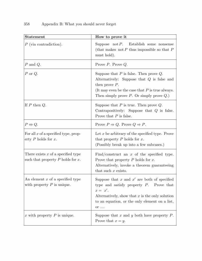
358 Appendix B: What you should never forget
Statement How to prove it
P (via contradiction). Suppose notP . Establish some nonsense
(that makes notP thus impossible so that P
must hold).
P and Q. Prove P . Prove Q.
P or Q. Suppose that P is false. Then prove Q.
Alternatively: Suppose that Q is false and
then prove P .
(It may even be the case that P is true always.
Then simply prove P . Or simply prove Q.)
If P then Q. Suppose that P is true. Then prove Q.
Contrapositively: Suppose that Q is false.
Prove that P is false.
P ⇔ Q. Prove P ⇒ Q. Prove Q⇒ P .
For all x of a specified type, prop-
erty P holds for x.
Let x be arbitrary of the specified type. Prove
that property P holds for x.
(Possibly break up into a few subcases.)
There exists x of a specified type
such that property P holds for x.
Find/construct an x of the specified type.
Prove that property P holds for x.
Alternatively, invoke a theorem guaranteeing
that such x exists.
An element x of a specified type
with property P is unique.
Suppose that x and x′ are both of specified
type and satisfy property P . Prove that
x = x′.
Alternatively, show that x is the only solution
to an equation, or the only element on a list,
or ....
x with property P is unique. Suppose that x and y both have property P .
Prove that x = y.

Appendix B: What you should never forget 359
Mathematical induction
The goal is to prove a property for all integers n ≥ n0. First prove the base case,
namely that the property holds for n0. For the inductive step, assume that for some
n− 1 ≥ n0, the property holds for n− 1 (alternatively, for n0, n0 + 1, . . . , n− 1), and then
prove the property for n.
The limit definition of derivative
f ′(a) = limh→0
f(a+ h)− f(a)
h= limx→a
f(x)− f(a)
x− a.
The limit-partition definition of integrals
A partition of [a, b] is a finite set P = {x0, x1, . . . , xn} such that x0 = a < x1 <
x2 < · · · < xn−1 < xn = b. Let f : [a, b]→ R be a bounded function. For each j = 1, . . . , n,
let
mj = inf{f(x) : x ∈ [xj−1, xj ]}, Mj = sup{f(x) : x ∈ [xj−1, xj ]}.
The lower sum of f with respect to P is
L(f, P ) =n∑j=1
mj(xj − xj−1).
The upper sum of f with respect to P is
U(f, P ) =n∑j=1
Mj(xj − xj−1).
The lower integral of f over [a,b] is
L(f) = sup{L(f, P ) : as P varies over partitions of [a, b]},
and the upper integral of f over [a,b] is
U(f) = inf{U(f, P ) : P varies over partitions of [a, b]}.
We say that f is integrable over [a, b] when L(f) = U(f). We call this common value
the integral of f over [a,b], and we write it as∫ b
a
f =
∫ b
a
f(x) dx =
∫ b
a
f(t) dt.
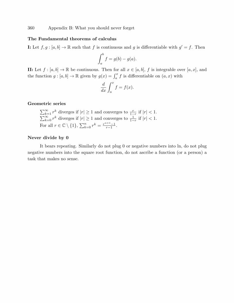
360 Appendix B: What you should never forget
The Fundamental theorems of calculus
I: Let f, g : [a, b]→ R such that f is continuous and g is differentiable with g′ = f . Then∫ b
a
f = g(b)− g(a).
II: Let f : [a, b]→ R be continuous. Then for all x ∈ [a, b], f is integrable over [a, x], and
the function g : [a, b]→ R given by g(x) =∫ xaf is differentiable on (a, x) with
d
dx
∫ x
a
f = f(x).
Geometric series∑∞k=1 r
k diverges if |r| ≥ 1 and converges to r1−r if |r| < 1.∑∞
k=0 rk diverges if |r| ≥ 1 and converges to 1
1−r if |r| < 1.
For all r ∈ C \ {1},∑nk=0 r
k = rn+1−1r−1 .
Never divide by 0
It bears repeating. Similarly do not plug 0 or negative numbers into ln, do not plug
negative numbers into the square root function, do not ascribe a function (or a person) a
task that makes no sense.

Index
SYMBOLS
◦ abstract binary operation 76
C 50, 133(nk
), n choose k 46
Ac complement of A 53
\ complement of sets 53
◦ composition of functions 68
cos 23
e (identity element for binary operation) 76
e: Euler’s constant 255
{} empty set 50
∅ empty set 50
∃ there exists 25
∀ for all 25
fn function composed with itself 68
sinn power of trigonometric function (not
composition) 68
> (strictly) greater than 86
≥ greater than or equal to 86
e (identity element for binary operation) 76
id (identity function) 66
⇔ if and only if 17
⇒ implies 15
∈ in a set 49
inf: infimum 87
∩ intersection 52
< (strictly) smaller than 86, 88, 89, 108
> (strictly) greater than 108
≥ greater than or equal to 108
≤ less than or equal to 86, 108
lim of sequence 270
lim inf 301
lim sup 301
ln: natural logarithm 253
¬ logical not 14
∨ logical or 15
∧ logical and 15
L(f, P ): lower sum 229
N 50
N0 101
± 98∏nk=1,
n∏k=1
product 36, 78
Q 50, 119
// end of proof 18
QED end of proof 18
end of proof 18
end of proof 18
R 50, 124
R≥0 50
Range: range of a function 65n√
195
sin 23, 24
⊆ subset of a set 51∑nk=1,
n∑k=1
34, 78
sup: supremum 87, 301
∪ union 52
U(f, P ): upper sum 229
Z 50, 113
00 35
A
Abel’s lemma 330
absolute value 19, 97
absolutely convergent 313
advice on writing proofs 353
alternating test for series 312
and (logical) 15
antecedent 15
antiderivative 246
arcsin, arccos, arctan 344

362 Index
area (signed or usual) 227
associative 77, 82, 83
axiom 101
B
base (of exponential function) 255
base case (of induction) 37, 41
base of exponentiation 195
Benjamin, A. 44
Bernoulli’s inequality 94
bijective function 68
composition 69
binary operation 76
associative 77
commutative 80
binomial (coefficient) 47
Boas, R. P. 347
Bombelli, R. 141
bounded function 228
bounded set 86
above 86
and open balls 151
below 86
Buck, R. C. 347
Bumcrot, R. J. 346
C
C 50, 133
absolute value 138
arithmetic 133
Cartesian coordinates 142
distance 138
length = norm = absolute value 138
polar coordinates 142
properties 134
reverse triangle inequality 139
triangle inequality 139
Campbell, P. J. 342
cancellation 80, 111, 118, 121
Cartesian coordinates 142
Cartesian product 59
Cauchy’s criterion for series 310
Cauchy’s mean value theorem 217, 218
ceiling function 72
chain rule 209
chart
how to prove 29, 358
negation 32, 357
choose: n choose k,(nk
)46
closed and bounded—contained in open
sets 152, 153
closed set 149
closed-form antiderivative 246
codomain (of a function) 65
commutative 80, 82, 83
comparison
sequences with infinite limits 279
sequences 285, 290
series 311
completeness of R, C 295
complex conjugate 137
complex number 133
with e 341
composition of functions 69
conditional statement 15
antecedent, consequent 15
beware 17
congruent modulo n 62
congruent modulo n 62
conjunction 15
connuousti 187
consequent 15
construction of N0 101
construction of Q from Z 65, 118
construction of R 124
construction of Z from N0 63
Index 363
contain 49
continuous 182
and inverse function 192
and monotonicity 192
connuousti 187
exponential function 198
exponentiation 196
image of interval 192
power series 331
properties 183
suounitnoc 186
ticonnuous 186
uniformly continuous 199, 219
convergent sequence 270
convergent
absolutely 313
convexity 217
cos: trigonometric function 23, 340
COS 337
D
Darboux’s theorem 215
de Moivre’s formula 342, 349
Dedekind cut 123
standard 131
definition: beware 17
degree (of polynomial) 35
derivative 202
and monotonicity 216
complex-valued functions 210
inverse 211
Leibniz’s notation 202
Newton’s notation 202
power rule for rational exponents 212
properties 207, 208, 209, 210, 211, 212
differentiable 202
hence continuous 206
Dirichlet’s test 316
disjunction 15
distributivity 82
division 83
do not divide by zero 84
domain (of a function) 65
implicit 67
E
e vs. π 258
Eantegral 237
element 49
empty product 36, 79
empty set 50
empty sum 35
enumeration of Q+ 267
epsilon-delta definition 154, 162
epsilon-N definition 180
equivalence (logical) 17
equivalence class 61, 112
equivalence relation 61, 112
Euclidean algorithm 39
Euclid 32
Euler’s constant (e) 255, 335
even function, its integral 72
even integer 25
definition 18
exclusive or (xor) 15
existential quantifier ∃ 25
exponential function 255
continuity 198
without derivatives and integrals 198
exponentiation 195
by real exponents 255
continuity 196
exponent 195, 255
Extreme value theorem 188

364 Index
F
Ferguson, S. J. 190
Fibonacci numbers 43, 266
field 82, 120, 128, 134
axioms 82
unusual 86
fixed point theorem 193
floor function 72
Fourier series 346
Fueter, R. 267
function 65
bijective 68
ceiling 72
codomain 65
composition 68
connuousti 187
constant 66
continuous 182
decreasing 95
domain 65
exponential 198, 255
floor 72
graph 65
identity 66
increasing 95
injective 68
monotone 95
inverse 95
one-to-one 68
onto 68
polynomial 35, 69
power 95
product of 85
radical 95, 195
range 65
rational 69
suounitnoc 186
surjective 68
ticonnuous 186
fundamental theorem of arithmetic 31
fundamental theorem of calculus 245, 247,
248
complex-valued 252, 253
G
Gaitanas, K. 42
generalized power function 255
generalized power series 322
geometric series 308
glb, inf: greatest lower bound 87
Goldbach’s conjecture 13
Greatest lower bound theorem 132
H
halving intervals 151
harmonic sequence 296
harmonic series 308
higher order derivatives 222
Hoseana, J. 176
how-to-prove chart 29, 358
I
identity element 76
additive 82, 83
multiplicative 82, 83
identity function 66
if and only if, iff 15
imaginary axis 134
imaginary part of a complex number 136
implication 15
improper integral 251, 252
indefinite integral 246
index (of unions, intersections) 52
induction 37, 102
base case 37, 41
Index 365
inductive step 37, 41
inductive set 101
infimum (inf, glb) 87
−∞ 301
infinite sequence: see sequence
infinite series: see series
injective function 68
composition 69
integer 92, 113
integrable 231, 241
integral test for series 313
integral 231
addition 242
applications 258
complex-valued function 252
double 350
monotonicity 244
notation 231, 233, 246, 248
integration by parts 250
integration by substitution 249
intermediate value theorem 191, 215
interval 49, 89
inverse 77, 95
additive 77, 83
derivative 211
multiplicative 77, 83
of a function 74
of a strictly monotone function 95
of product 79
unique 78
invertible (element) 78
invertible (function) 74
J
joke 28
L
L’Hopital’s rule at infinity 222, 257, 347
L’Hopital’s rule 219, 220, 257, 258, 346
Lagrange interpolation 75
least element 88, 94, 109
Least upper bound theorem 132
least upper bound: lub, supremum, sup 87
Leibniz, G. 141
lemma: helpful theorem 111
length of curve 259
limit inferior, liminf 301
limit point (of set) 149
limit superior, limsup 301
limit
absolute value 172
at infinity 180
composite function theorem 173
epsilon-delta definition 154, 162
epsilon-N definition 180
infinite 176
M-delta definition 176
M-N definition 180
of a function 154, 162, 176, 180
of sequence 270
polynomial rule 171
power rule 171
rational rule 172
real/imaginary part 172
right/left-handed 162, 176
squeeze theorem 173
subsequence 299
theorems for infinite limits 178
theorems 169, 171, 172, 173
uniqueness 168
ln, natural logarithm 253
inverse 335
logarithmic differentiation 257
logic circuits 23
366 Index
logical biconditional 17
logic 13, 25, 28
lower bound of set 86
lower integral 231
lower sum (integrals) 229
lub, sup: see least upper bound
M
Matsuoka, Y. 348
mean value theorem for integrals 250
mean value theorem 216
member (of a set) 49
Mestrovic, R. 33
modulo n 62
modus ponens 19
monotone function 95
and derivative 216
monotone sequence 291, 294
N
N 50
N0 101, 106
natural logarithm, ln 253
natural number (in N0) 101
negation 14, 32
chart 32, 357
negative 89, 117, 122, 132
Nelson, E. 186
non-negative 89, 117, 122, 132
non-positive 89, 117, 122, 132
not: see negation
notation
integral 246, 248
set vs. sequence 265
number of elements in Q+ 75
O
odd function, its integral 72
odd integer 25
definition 18
one-to-one 68
onto 68
open ball 147
open set 147
or (logical) 15
ordered pair 58
ordered set 89
field 89
order 86
N0 108
Q 121
R 131
Z 116
P
p-test for series 314
Papadimitriou, I. 349
partial sum (of a sequence) 306, 307
partition (of an interval) 228
refinement 230
partition
sub-interval 228
Pascal’s triangle 46
π vs. e 258π2
6 348, 350
pigeonhole principle 73
polar coordinates 142
polynomial function 35, 69, 70, 71, 137,
171, 223, 284, 289
degree 35
Taylor polynomial 223
popcorn function 186
positive 89, 117, 122, 132
power function 95, 96, 171, 194, 284, 289
Index 367
generalized 196, 255
power notation 35, 68, 79
00 35
for functions 68, 82
on sets with binary operation 79
special in trigonometry 68
power rule for derivatives 208
power rule
generalized 212
power series—generalized 322
power series 317, 322
continuous 331
derivative 324
inverse 330
numerical evaluation 325
product of two 327
radius of convergence 319
ratio test 320
root test 318
Taylor series 331
uniqueness 324
prime 13, 30, 31, 32
definition 17, 18
principle of mathematical induction 37
principle
do not divide by zero
product∏nk=1 36, 78
product (not composition) of functions 85
product rule for derivatives 207
product rule for higher derivatives 225
proof 18, 28
by contradiction 21
by induction 37
deductive reasoning 18
how-to-prove chart 29, 358
pigeonhole principle 73√2 is not rational 21
proper subset 51
Pythagoras 21
Polya, G. 267
Q
Q 50, 119
Archimedean property 122
cancellation 121
field 120
ordered 121
QED (quod erat demonstrandum) 18
quadratic formula 23, 70
quantifier
existential 25
universal 25
quartering subsets 151
quotient rule for derivatives 207
quotient rule for higher derivatives 226
R
R 50, 124
Archimedean property 132
field 128
ordered 131
properties 128, 132
Raabe’s test 317
radical function 95, 195
radius of convergence (of power series) 319
range (of a function) 65
ratio test
for power series 320
for sequences 292, 302
for series 311
rational function 137
rational number (in Q) 119
rational numbers between real numbers
132
rational number 21, 92
real axis 134
368 Index
real number 124
real part of a complex number 136
recursive 266
refinement (of a partition) 230
relation on sets 60
equivalence 61
reflexive 61
symmetric 61
transitive 61
restriction of a function 183
reverse triangle inequality 98, 132, 139
Ritelli, D. 350
Rolle’s theorem 215
root of a number 195
root test for power series 318
root test for series 312
S
Sagher, Y. 75
second derivative test 225
sequence vs. set notation 265
sequence 265
arithmetic on sequences 268
bounded (below/above) 291
Cauchy 294
comparison for infinite limits 279
comparison 285, 290
completeness of R, C 295
composite rule 284, 289
constant 265
convergence 270, 287
properties 282, 284, 288, 289
divergence to ±∞ 279
divergence 278
Fibonacci 266
finite 269
limit 270
unique 282, 288
monotone 291, 294
of partial sums 306, 307
ratio test 292, 302
squeeze theorem 286, 290
subsequence 298
term 265
series
alternating test 312
arithmetic with 307
comparison 311
converges 307
diverges 307
geometric 308
harmonic 308
integral test 313
numerical evaluation 325
p-series test 314
power 317, 322
ratio test 311, 320
root test 312, 318
set vs. sequence notation 265
set 49
complement 53
disjoint 52
empty set 50
equality 52
intersection 52
member 49
notation 49
propositionally 50
subset 51
sum of 91
union 52
universal 53
signed area 227, 229
sin: trigonometric function 23, 24, 340
SIN 337
socks-and-shoes 81
Index 369
spiral of Theodorus 44
statement 13
conditional statement 15
conjunction 15
disjunction 15
equivalence 17
if and only if 15
implication 15
logical biconditional 17
negation 14
xor 15
sub-interval of a partition 228
subsequence 298
subsequential limit 299
subset 51
subtraction 83
successor 101
sum of sets 91
summation∑nk=1 34, 78
summation by parts 316
suounitnoc 186
supremum (sup, lub) 87
∞ 301
surface area of a surface of revolution 261
surjective function 68
composition 69
T
tautology 18
Taylor polynomial 223, 257
Taylor series 331
not approximating 334
Taylor’s remainder theorem 224, 225, 251
Thomae function 186
ticonnuous 186
topology 147, 148, 149
closed set 149
limit point 149
open ball 147
open set 147
tower of Hanoi 45
triangle inequality 20, 98
over C 139
reverse 98, 132, 139
trichotomy (of <) 88, 109, 116
trigonometry 340
tromino 44
truth table 14, 357
U
uniform continuity 199
uniformly continuity 219
universal quantifier ∀ 25
universal set 53
unusual field 86
upper bound of set 86
upper integral 231
upper sum (integrals) 229
V
vacuously true 26
Velleman, D. 44, 348
Venn diagram 55
volume of a surface of revolution 260
Vorob’ev, N. N. 43
W
well-defined 75
well-ordered 88, 94, 109
whole number 113
X
xor 15
370 Index
Z
Z 50, 113
properties 114, 116
zero: do not divide by it 9, 84, 353
zeroth derivative 222
zeroth power 35