introduction to articial intelligence problem solving and...
TRANSCRIPT
Introduction to Artificial Intelligence
Problem Solving and Search
Bernhard Beckert
UNIVERSITÄT KOBLENZ-LANDAU
Winter Term 2004/2005
B. Beckert: KI für IM – p.1

Outline
Problem solving
Problem types
Problem formulation
Example problems
Basic search algorithms
B. Beckert: KI für IM – p.2

Problem solving
Offline problem solving
Acting only with complete knowledge of problem and solution
Online problem solving
Acting without complete knowledge
Here
Here we are concerned with offline problem solving only
B. Beckert: KI für IM – p.3

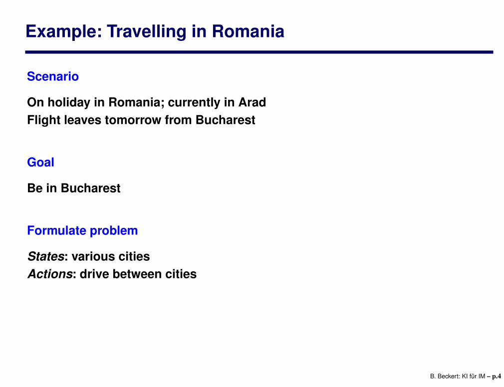
Example: Travelling in Romania
Scenario
On holiday in Romania; currently in AradFlight leaves tomorrow from Bucharest
Goal
Be in Bucharest
Formulate problem
States: various citiesActions: drive between cities
Solution
Appropriate sequence of citiese.g.: Arad, Sibiu, Fagaras, Bucharest
B. Beckert: KI für IM – p.4

Example: Travelling in Romania
Giurgiu
UrziceniHirsova
Eforie
Neamt
Oradea
Zerind
Arad
Timisoara
Lugoj
Mehadia
Dobreta
Craiova
Sibiu Fagaras
Pitesti
Vaslui
Iasi
Rimnicu Vilcea
Bucharest
B. Beckert: KI für IM – p.5

Problem types
Single-state problem
– observable (at least the initial state)– deterministic– static– discrete
Multiple-state problem
– partially observable (initial state not observable)– deterministic– static– discrete
Contingency problem
– partially observable (initial state not observable)– non-deterministic
B. Beckert: KI für IM – p.6

Example: vacuum-cleaner world
Single-state
Start in: 5
Solution:
[right, suck ]
Multiple-state
Start in: {1,2,3,4,5,6,7,8}
Solution: [right, suck, left, suck ]
right → {2,4,6,8}
suck → {4,8}
left → {3,7}
suck → {7}
1 2
3 4
5 6
7 8
B. Beckert: KI für IM – p.7

Example: vacuum-cleaner world
Single-state
Start in: 5
Solution: [right, suck ]
Multiple-state
Start in: {1,2,3,4,5,6,7,8}
Solution: [right, suck, left, suck ]
right → {2,4,6,8}
suck → {4,8}
left → {3,7}
suck → {7}
1 2
3 4
5 6
7 8
B. Beckert: KI für IM – p.7

Example: vacuum-cleaner world
Single-state
Start in: 5
Solution: [right, suck ]
Multiple-state
Start in: {1,2,3,4,5,6,7,8}
Solution:
[right, suck, left, suck ]
right → {2,4,6,8}
suck → {4,8}
left → {3,7}
suck → {7}
1 2
3 4
5 6
7 8
B. Beckert: KI für IM – p.7

Example: vacuum-cleaner world
Single-state
Start in: 5
Solution: [right, suck ]
Multiple-state
Start in: {1,2,3,4,5,6,7,8}
Solution: [right, suck, left, suck ]
right → {2,4,6,8}
suck → {4,8}
left → {3,7}
suck → {7}
1 2
3 4
5 6
7 8
B. Beckert: KI für IM – p.7

Example: vacuum-cleaner world
Contingency
Murphy’s Law:suck can dirty a clean carpet
Local sensing:dirty /not dirty at location only
Start in: {1,3}
Solution:
[suck, right, suck ]
suck → {5,7}
right → {6,8}
suck → {6,8}
Improvement: [suck, right, if dirt then suck ](decide whether in 6 or 8 using local sensing)
1 2
3 4
5 6
7 8
B. Beckert: KI für IM – p.8

Example: vacuum-cleaner world
Contingency
Murphy’s Law:suck can dirty a clean carpet
Local sensing:dirty /not dirty at location only
Start in: {1,3}
Solution: [suck, right, suck ]
suck → {5,7}
right → {6,8}
suck → {6,8}
Improvement: [suck, right, if dirt then suck ](decide whether in 6 or 8 using local sensing)
1 2
3 4
5 6
7 8
B. Beckert: KI für IM – p.8

Single-state problem formulation
Defined by the following four items
1. Initial state
Example: Arad
2. Successor function S
Example: S(Arad) = { 〈goZerind,Zerind〉, 〈goSibiu,Sibiu〉, . . . }
3. Goal test
Example: x = Bucharest (explicit test)
noDirt(x) (implicit test)
4. Path cost (optional)
Example: sum of distances, number of operators executed, etc.
B. Beckert: KI für IM – p.9

Single-state problem formulation
Solution
A sequence of operatorsleading from the initial state to a goal state
B. Beckert: KI für IM – p.10

Selecting a state space
Abstraction
Real world is absurdly complexState space must be abstracted for problem solving
(Abstract) state
Set of real states
(Abstract) operator
Complex combination of real actionsExample: Arad→ Zerind represents complex set of possible routes
(Abstract) solution
Set of real paths that are solutions in the real world
B. Beckert: KI für IM – p.11

Example: The 8-puzzle
2
Start State Goal State
51 3
4 6
7 8
5
1
2
3
4
6
7
8
5
States
integer locations of tiles
Actions
left, right, up, down
Goal test
= goal state?
Path cost
1 per move
B. Beckert: KI für IM – p.12

Example: The 8-puzzle
2
Start State Goal State
51 3
4 6
7 8
5
1
2
3
4
6
7
8
5
States integer locations of tiles
Actions
left, right, up, down
Goal test
= goal state?
Path cost
1 per move
B. Beckert: KI für IM – p.12

Example: The 8-puzzle
2
Start State Goal State
51 3
4 6
7 8
5
1
2
3
4
6
7
8
5
States integer locations of tiles
Actions left, right, up, down
Goal test
= goal state?
Path cost
1 per move
B. Beckert: KI für IM – p.12

Example: The 8-puzzle
2
Start State Goal State
51 3
4 6
7 8
5
1
2
3
4
6
7
8
5
States integer locations of tiles
Actions left, right, up, down
Goal test = goal state?
Path cost
1 per move
B. Beckert: KI für IM – p.12

Example: The 8-puzzle
2
Start State Goal State
51 3
4 6
7 8
5
1
2
3
4
6
7
8
5
States integer locations of tiles
Actions left, right, up, down
Goal test = goal state?
Path cost 1 per move
B. Beckert: KI für IM – p.12

Example: Vacuum-cleaner
R
L
S S
S S
R
L
R
L
R
L
S
SS
S
L
L
LL R
R
R
R
States
integer dirt and robot locations
Actions
left, right, suck, noOp
Goal test
not dirty?
Path cost
1 per operation (0 for noOp)
B. Beckert: KI für IM – p.13

Example: Vacuum-cleaner
R
L
S S
S S
R
L
R
L
R
L
S
SS
S
L
L
LL R
R
R
R
States integer dirt and robot locations
Actions
left, right, suck, noOp
Goal test
not dirty?
Path cost
1 per operation (0 for noOp)
B. Beckert: KI für IM – p.13

Example: Vacuum-cleaner
R
L
S S
S S
R
L
R
L
R
L
S
SS
S
L
L
LL R
R
R
R
States integer dirt and robot locations
Actions left, right, suck, noOp
Goal test
not dirty?
Path cost
1 per operation (0 for noOp)
B. Beckert: KI für IM – p.13

Example: Vacuum-cleaner
R
L
S S
S S
R
L
R
L
R
L
S
SS
S
L
L
LL R
R
R
R
States integer dirt and robot locations
Actions left, right, suck, noOp
Goal test not dirty?
Path cost
1 per operation (0 for noOp)
B. Beckert: KI für IM – p.13

Example: Vacuum-cleaner
R
L
S S
S S
R
L
R
L
R
L
S
SS
S
L
L
LL R
R
R
R
States integer dirt and robot locations
Actions left, right, suck, noOp
Goal test not dirty?
Path cost 1 per operation (0 for noOp)
B. Beckert: KI für IM – p.13

Example: Robotic assembly
R
RRP
R R
States
real-valued coordinates of
robot joint angles and parts of the object to be assembled
Actions
continuous motions of robot joints
Goal test
assembly complete?
Path cost
time to execute
B. Beckert: KI für IM – p.14

Example: Robotic assembly
R
RRP
R R
States real-valued coordinates of
robot joint angles and parts of the object to be assembled
Actions
continuous motions of robot joints
Goal test
assembly complete?
Path cost
time to execute
B. Beckert: KI für IM – p.14

Example: Robotic assembly
R
RRP
R R
States real-valued coordinates of
robot joint angles and parts of the object to be assembled
Actions continuous motions of robot joints
Goal test
assembly complete?
Path cost
time to execute
B. Beckert: KI für IM – p.14

Example: Robotic assembly
R
RRP
R R
States real-valued coordinates of
robot joint angles and parts of the object to be assembled
Actions continuous motions of robot joints
Goal test assembly complete?
Path cost
time to execute
B. Beckert: KI für IM – p.14

Example: Robotic assembly
R
RRP
R R
States real-valued coordinates of
robot joint angles and parts of the object to be assembled
Actions continuous motions of robot joints
Goal test assembly complete?
Path cost time to executeB. Beckert: KI für IM – p.14

Tree search algorithms
Offline
Simulated exploration of state space in a search treeby generating successors of already-explored states
function TREE-SEARCH( problem, strategy) returns a solution or failure
initialize the search tree using the initial state of problem
loop do
if there are no candidates for expansion then return failure
choose a leaf node for expansion according to strategy
if the node contains a goal state thenreturn the corresponding solution
else
expand the node and add the resulting nodes to the search tree
end
B. Beckert: KI für IM – p.15

Tree search: Example
Rimnicu Vilcea Lugoj
ZerindSibiu
Arad Fagaras Oradea
Timisoara
AradArad Oradea
Arad
B. Beckert: KI für IM – p.16

Tree search: Example
Rimnicu Vilcea LugojArad Fagaras Oradea AradArad Oradea
Zerind
Arad
Sibiu Timisoara
B. Beckert: KI für IM – p.16

Tree search: Example
Lugoj AradArad OradeaRimnicu Vilcea
Zerind
Arad
Sibiu
Arad Fagaras Oradea
Timisoara
B. Beckert: KI für IM – p.16

Implementation: States vs. nodes
State
A (representation of) a physical configuration
Node
A data structure constituting part of a search tree(includes parent, children, depth, path cost, etc.)
1
23
45
6
7
81
23
45
6
7
8
State Node
parent
depth = 6
g = 6
childrenstate
B. Beckert: KI für IM – p.17

Implementation of search algorithms
function TREE-SEARCH( problem, fringe) returns a solution or failure
fringe← INSERT(MAKE-NODE(INITIAL-STATE[problem]),fringe)
loop do
if fringe is empty then return failure
node← REMOVE-FIRST(fringe)
if GOAL-TEST[problem] applied to STATE(node) succeeds then
return node
else
fringe← INSERT-ALL(EXPAND(node, problem), fringe)
end
fringe queue of nodes not yet consideredState gives the state that is represented by nodeExpand creates new nodes by applying possible actions to node
B. Beckert: KI für IM – p.18

Search strategies
Strategy
Defines the order of node expansion
Important properties of strategies
completeness does it always find a solution if one exists?
time complexity number of nodes generated/expanded
space complexity maximum number of nodes in memory
optimality does it always find a least-cost solution?
Time and space complexity measured in terms of
b maximum branching factor of the search tree
d depth of a solution with minimal distance to root
m maximum depth of the state space (may be ∞)
B. Beckert: KI für IM – p.19

Uninformed search strategies
Uninformed search
Use only the information available in the problem definition
Frequently used strategies
Breadth-first search
Uniform-cost search
Depth-first search
Depth-limited search
Iterative deepening search
B. Beckert: KI für IM – p.20

Breadth-first search
Idea
Expand shallowest unexpanded node
Implementation
fringe is a FIFO queue, i.e. successors go in at the end of the queue
A
B C
D E F GB. Beckert: KI für IM – p.21

Breadth-first search
Idea
Expand shallowest unexpanded node
Implementation
fringe is a FIFO queue, i.e. successors go in at the end of the queue
A
B C
D E F GB. Beckert: KI für IM – p.21

Breadth-first search
Idea
Expand shallowest unexpanded node
Implementation
fringe is a FIFO queue, i.e. successors go in at the end of the queue
A
B C
D E F GB. Beckert: KI für IM – p.21

Breadth-first search
Idea
Expand shallowest unexpanded node
Implementation
fringe is a FIFO queue, i.e. successors go in at the end of the queue
A
B C
D E F GB. Beckert: KI für IM – p.21

Breadth-first search: Example Romania
Arad
B. Beckert: KI für IM – p.22

Breadth-first search: Example Romania
Zerind Sibiu Timisoara
Arad
B. Beckert: KI für IM – p.22

Breadth-first search: Example Romania
Arad Oradea
Zerind Sibiu Timisoara
Arad
B. Beckert: KI für IM – p.22

Breadth-first search: Example Romania
Arad Oradea Rimnicu VilceaFagaras Arad LugojArad Oradea
Zerind Sibiu Timisoara
Arad
B. Beckert: KI für IM – p.22

Breadth-first search: Properties
Complete
Yes (if b is finite)
Time
1+b+b2 +b3 + . . .+bd +b(bd−1) ∈ O(bd+1)
i.e. exponential in d
Space
O(bd+1)
keeps every node in memory
Optimal
Yes (if cost = 1 per step), not optimal in general
Disadvantage
Space is the big problem(can easily generate nodes at 5MB/sec so 24hrs = 430GB)
B. Beckert: KI für IM – p.23

Breadth-first search: Properties
Complete Yes (if b is finite)
Time 1+b+b2 +b3 + . . .+bd +b(bd−1) ∈ O(bd+1)
i.e. exponential in d
Space O(bd+1)
keeps every node in memory
Optimal Yes (if cost = 1 per step), not optimal in general
Disadvantage
Space is the big problem(can easily generate nodes at 5MB/sec so 24hrs = 430GB)
B. Beckert: KI für IM – p.23

Romania with step costs in km
Bucharest
Giurgiu
Urziceni
Hirsova
Eforie
NeamtOradea
Zerind
Arad
Timisoara
LugojMehadia
DobretaCraiova
Sibiu
Fagaras
PitestiRimnicu Vilcea
Vaslui
Iasi
Straight−line distanceto Bucharest
0160242161
77151
241
366
193
178
253329
80199
244
380
226
234
374
98
Giurgiu
UrziceniHirsova
Eforie
Neamt
Oradea
Zerind
Arad
Timisoara
Lugoj
Mehadia
Dobreta
Craiova
Sibiu Fagaras
Pitesti
Vaslui
Iasi
Rimnicu Vilcea
Bucharest
71
75
118
111
70
75120
151
140
99
80
97
101
211
138
146 85
90
98
142
92
87
86
B. Beckert: KI für IM – p.24

Uniform-cost search
Idea
Expand least-cost unexpanded node(costs added up over paths from root to leafs)
Implementation
fringe is queue ordered by increasing path cost
Note
Equivalent to depth-first search if all step costs are equal
B. Beckert: KI für IM – p.25

Uniform-cost search
Arad
B. Beckert: KI für IM – p.26

Uniform-cost search
Zerind Sibiu Timisoara
75 140 118
Arad
B. Beckert: KI für IM – p.26

Uniform-cost search
Arad Oradea
75 71
Zerind Sibiu Timisoara
75 140 118
Arad
B. Beckert: KI für IM – p.26

Uniform-cost search
Arad Lugoj
118 111
Arad Oradea
75 71
Zerind Sibiu Timisoara
75 140 118
Arad
B. Beckert: KI für IM – p.26

Uniform-cost search: Properties
Complete
Yes (if step costs positive)
Time
# of nodes with past-cost less than that of optimal solution
Space
# of nodes with past-cost less than that of optimal solution
Optimal
Yes
B. Beckert: KI für IM – p.27

Uniform-cost search: Properties
Complete Yes (if step costs positive)
Time
# of nodes with past-cost less than that of optimal solution
Space
# of nodes with past-cost less than that of optimal solution
Optimal
Yes
B. Beckert: KI für IM – p.27

Uniform-cost search: Properties
Complete Yes (if step costs positive)
Time # of nodes with past-cost less than that of optimal solution
Space
# of nodes with past-cost less than that of optimal solution
Optimal
Yes
B. Beckert: KI für IM – p.27

Uniform-cost search: Properties
Complete Yes (if step costs positive)
Time # of nodes with past-cost less than that of optimal solution
Space # of nodes with past-cost less than that of optimal solution
Optimal
Yes
B. Beckert: KI für IM – p.27

Uniform-cost search: Properties
Complete Yes (if step costs positive)
Time # of nodes with past-cost less than that of optimal solution
Space # of nodes with past-cost less than that of optimal solution
Optimal Yes
B. Beckert: KI für IM – p.27

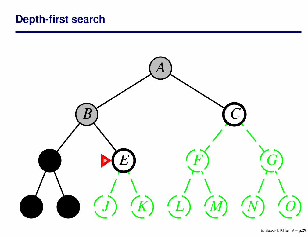
Depth-first search
Idea
Expand deepest unexpanded node
Implementation
fringe is a LIFO queue (a stack), i.e. successors go in at front of queue
Note
Depth-first search can perform infinite cyclic excursions
Need a finite, non-cyclic search space (or repeated-state checking)
B. Beckert: KI für IM – p.28

Depth-first search
A
B C
D E F G
H I J K L M N OB. Beckert: KI für IM – p.29

Depth-first search
A
B C
D E F G
H I J K L M N OB. Beckert: KI für IM – p.29

Depth-first search
A
B C
D E F G
H I J K L M N OB. Beckert: KI für IM – p.29

Depth-first search
A
B C
D E F G
H I J K L M N O
B. Beckert: KI für IM – p.29

Depth-first search
A
B C
D E F G
H I J K L M N OB. Beckert: KI für IM – p.29
Depth-first search
A
B C
D E F G
H I J K L M N OB. Beckert: KI für IM – p.29

Depth-first search
A
B C
D E F G
H I J K L M N OB. Beckert: KI für IM – p.29

Depth-first search
A
B C
D E F G
H I J K L M N OB. Beckert: KI für IM – p.29

Depth-first search
A
B C
D E F G
H I J K L M N OB. Beckert: KI für IM – p.29

Depth-first search
A
B C
D E F G
H I J K L M N OB. Beckert: KI für IM – p.29

Depth-first search
A
B C
D E F G
H I J K L M N OB. Beckert: KI für IM – p.29

Depth-first search
A
B C
D E F G
H I J K L M N OB. Beckert: KI für IM – p.29

Depth-first search: Example Romania
Arad
B. Beckert: KI für IM – p.30

Depth-first search: Example Romania
Zerind Sibiu Timisoara
Arad
B. Beckert: KI für IM – p.30

Depth-first search: Example Romania
Arad Oradea
Zerind Sibiu Timisoara
Arad
B. Beckert: KI für IM – p.30
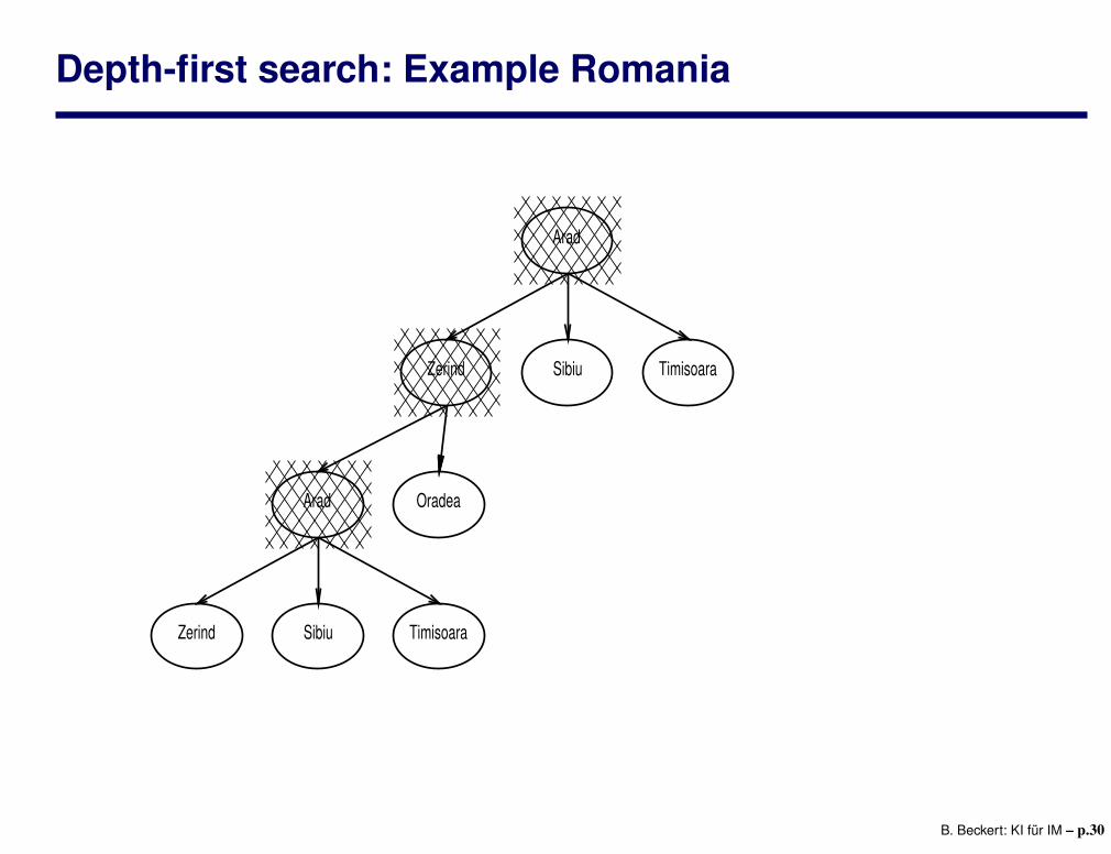
Depth-first search: Example Romania
Zerind Sibiu Timisoara
Arad Oradea
Zerind Sibiu Timisoara
Arad
B. Beckert: KI für IM – p.30

Depth-first search: Properties
Complete
Yes: if state space finite
No: if state contains infinite paths or loops
Time
O(bm)
Space
O(bm) (i.e. linear space)
Optimal
No
Disadvantage
Time terrible if m much larger than d
Advantage
Time may be much less than breadth-first search if solutions are dense
B. Beckert: KI für IM – p.31

Depth-first search: Properties
Complete Yes: if state space finite
No: if state contains infinite paths or loops
Time O(bm)
Space O(bm) (i.e. linear space)
Optimal No
Disadvantage
Time terrible if m much larger than d
Advantage
Time may be much less than breadth-first search if solutions are dense
B. Beckert: KI für IM – p.31

Iterative deepening search
Depth-limited search
Depth-first search with depth limit
Iterative deepening search
Depth-limit search with ever increasing limits
function ITERATIVE-DEEPENING-SEARCH( problem) returns a solution or failure
inputs: problem /* a problem */
for depth← 0 to ∞ do
result← DEPTH-LIMITED-SEARCH( problem, depth)
if result 6= cutoff then return result
end
B. Beckert: KI für IM – p.32

Iterative deepening search
Depth-limited search
Depth-first search with depth limit
Iterative deepening search
Depth-limit search with ever increasing limits
function ITERATIVE-DEEPENING-SEARCH( problem) returns a solution or failure
inputs: problem /* a problem */
for depth← 0 to ∞ do
result← DEPTH-LIMITED-SEARCH( problem, depth)
if result 6= cutoff then return result
end
B. Beckert: KI für IM – p.32

Iterative deepening search with depth limit 0
Limit = 0 A A
B. Beckert: KI für IM – p.33

Iterative deepening search with depth limit 1
Limit = 1 A
B C
A
B C
A
B C
A
B C
B. Beckert: KI für IM – p.34

Iterative deepening search with depth limit 2
Limit = 2 A
B C
D E F G
A
B C
D E F G
A
B C
D E F G
A
B C
D E F G
A
B C
D E F G
A
B C
D E F G
A
B C
D E F G
A
B C
D E F G
B. Beckert: KI für IM – p.35

Iterative deepening search with depth limit 3
Limit = 3
A
B C
D E F G
H I J K L M N O
A
B C
D E F G
H I J K L M N O
A
B C
D E F G
H I J K L M N O
A
B C
D E F G
H I J K L M N O
A
B C
D E F G
H I J K L M N O
A
B C
D E F G
H I J K L M N O
A
B C
D E F G
H I J K L M N O
A
B C
D E F G
H I J K L M N O
A
B C
D E F G
H I J K L M N O
A
B C
D E F G
H I J K L M N O
A
B C
D E F G
H J K L M N OI
A
B C
D E F G
H I J K L M N O
B. Beckert: KI für IM – p.36

Iterative deepening search: Example Romania with l = 0
Arad
B. Beckert: KI für IM – p.37

Iterative deepening search: Example Romania with l = 1
Arad
B. Beckert: KI für IM – p.38

Iterative deepening search: Example Romania with l = 1
Zerind Sibiu Timisoara
Arad
B. Beckert: KI für IM – p.38

Iterative deepening search: Example Romania with l = 2
Arad
B. Beckert: KI für IM – p.39

Iterative deepening search: Example Romania with l = 2
Zerind Sibiu Timisoara
Arad
B. Beckert: KI für IM – p.39

Iterative deepening search: Example Romania with l = 2
Arad Oradea
Zerind Sibiu Timisoara
Arad
B. Beckert: KI für IM – p.39

Iterative deepening search: Example Romania with l = 2
Arad Oradea Rimnicu VilceaFagarasArad Oradea
Zerind Sibiu Timisoara
Arad
B. Beckert: KI für IM – p.39

Iterative deepening search: Example Romania with l = 2
Arad LugojArad Oradea Rimnicu VilceaFagarasArad Oradea
Zerind Sibiu Timisoara
Arad
B. Beckert: KI für IM – p.39

Iterative deepening search: Properties
Complete
Yes
Time
(d +1)b0 +db1 +(d−1)b2 + . . .+bd ∈ O(bd+1)
Space
O(bd)
Optimal
Yes (if step cost = 1)
(Depth-First) Iterative-Deepening Search often used in practice for
search spaces of large, infinite, or unknown depth.
B. Beckert: KI für IM – p.40

Iterative deepening search: Properties
Complete Yes
Time
(d +1)b0 +db1 +(d−1)b2 + . . .+bd ∈ O(bd+1)
Space
O(bd)
Optimal
Yes (if step cost = 1)
(Depth-First) Iterative-Deepening Search often used in practice for
search spaces of large, infinite, or unknown depth.
B. Beckert: KI für IM – p.40
Iterative deepening search: Properties
Complete Yes
Time (d +1)b0 +db1 +(d−1)b2 + . . .+bd ∈ O(bd+1)
Space
O(bd)
Optimal
Yes (if step cost = 1)
(Depth-First) Iterative-Deepening Search often used in practice for
search spaces of large, infinite, or unknown depth.
B. Beckert: KI für IM – p.40

Iterative deepening search: Properties
Complete Yes
Time (d +1)b0 +db1 +(d−1)b2 + . . .+bd ∈ O(bd+1)
Space O(bd)
Optimal
Yes (if step cost = 1)
(Depth-First) Iterative-Deepening Search often used in practice for
search spaces of large, infinite, or unknown depth.
B. Beckert: KI für IM – p.40

Iterative deepening search: Properties
Complete Yes
Time (d +1)b0 +db1 +(d−1)b2 + . . .+bd ∈ O(bd+1)
Space O(bd)
Optimal Yes (if step cost = 1)
(Depth-First) Iterative-Deepening Search often used in practice for
search spaces of large, infinite, or unknown depth.
B. Beckert: KI für IM – p.40

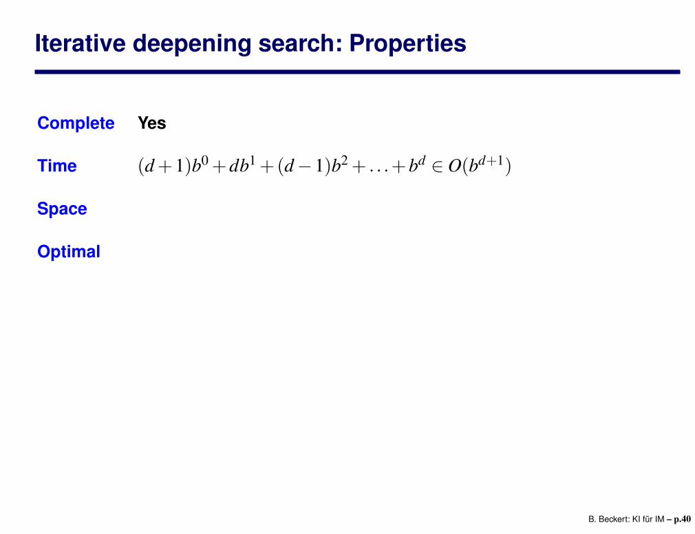
Iterative deepening search: Properties
Complete Yes
Time (d +1)b0 +db1 +(d−1)b2 + . . .+bd ∈ O(bd+1)
Space O(bd)
Optimal Yes (if step cost = 1)
(Depth-First) Iterative-Deepening Search often used in practice for
search spaces of large, infinite, or unknown depth.
B. Beckert: KI für IM – p.40

Comparison
CriterionBreadth-
firstUniform-
costDepth-
firstIterative
deepening
Complete? Yes∗ Yes∗ No Yes
Time bd+1 ≈ bd bm bd
Space bd+1 ≈ bd bm bd
Optimal? Yes∗ Yes No Yes
B. Beckert: KI für IM – p.41

Comparison
Breadth-first search Iterative deepening search
B. Beckert: KI für IM – p.42

Summary
Problem formulation usually requires abstracting away real-world detailsto define a state space that can feasibly be explored
Variety of uninformed search strategies
Iterative deepening search uses only linear spaceand not much more time than other uninformed algorithms
B. Beckert: KI für IM – p.43