rainfall prediction by articial neural networks trained
TRANSCRIPT

Rainfall Prediction by Arti�cial Neural NetworksTrained using Different Climate VariablesMateus Alexandre da Silva ( [email protected] )
Federal University of Lavras https://orcid.org/0000-0002-2849-0668Marina Neves Merlo
Federal University of LavrasMichael Silveira Thebaldi
Federal University of LavrasDanton Diego Ferreira
Federal University of LavrasFelipe Schwerz
Federal University of LavrasFábio Ponciano de Deus
Federal University of Lavras
Research Article
Keywords: Rainfall prediction, arti�cial neural networks, climate variables
Posted Date: June 22nd, 2021
DOI: https://doi.org/10.21203/rs.3.rs-569733/v1
License: This work is licensed under a Creative Commons Attribution 4.0 International License. Read Full License
Rainfall prediction by artificial neural networks trained using different climate variables
Mateus Alexandre da Silva¹, Marina Neves Merlo¹, Michael Silveira Thebaldi¹, Danton Diego Ferreira², Felipe
Schwerz³ and Fábio Ponciano de Deus¹
¹ Department of Water Resources, Federal University of Lavras, University Campus, Mailbox 3037, Lavras,
Minas Gerais, Brazil. ZIP CODE: 37.200-900.
(E-mail: [email protected], [email protected], [email protected],
[email protected]; Orcid: 0000-0002-2849-0668, 0000-0002-9518-6033, 0000-0002-4579-6714, 0000-
0002-9428-0095)
² Automation Department, Federal University of Lavras, University Campus, Mailbox 3037, Lavras, Minas
Gerais, Brazil. ZIP CODE: 37.200-900. (E-mail: [email protected]; Orcid: 0000-0002-4504-7721)
³ Department of Agricultural Engineering, Federal University of Lavras, University Campus, Mailbox 3037,
Lavras, Minas Gerais, Brazil. ZIP CODE: 37.200-900. (E-mail: [email protected]; Orcid: 0000-0001-
5266-4309)
Corresponding author: Mateus Alexandre da Silva (e-mail: [email protected])
Abstract
Predicting rainfall can prevent and mitigate damages caused by its deficit or excess, besides providing
necessary tools for adequate planning for the use of water. This research aimed to predict the monthly rainfall,
one month in advance, in four municipalities in the metropolitan region of Belo Horizonte, using artificial
neural networks (ANN) trained with different climate variables, and to indicate the suitability of such variables
as inputs to these models. The models were developed through the MATLAB® software version R2011a,
using the NNTOOL toolbox. The ANN’s were trained by the multilayer perceptron architecture and the
Feedforward and Back propagation algorithm, using two combinations of input data were used, with 2 and 6
variables, and one combination of input data with 3 of the 6 variables most correlated to observed rainfall from
1970 to 1999, to predict the rainfall from 2000 to 2009. The most correlated variables to the rainfall of the
following month are the sequential number corresponding to the month, total rainfall and average compensated
temperature, and the best performance was obtained with these variables. Furthermore, it was concluded that
the performance of the models was satisfactory; however, they presented limitations for predicting months with
high rainfall.
Declarations
Funding: This study was financed in part by the Coordenação de Aperfeiçoamento de Pessoal de Nível
Superior – Brasil (CAPES) – Finance Code 001.
Acknowledgments: The authors would like to thank the Coordenação de Aperfeiçoamento de Pessoal de Nível
Superior – Brasil (CAPES) for funding this research.
Conflicts of interest/Competing interests: The authors have no relevant financial or non-financial interests
to disclose.
Availability of data and material: The datasets generated or analysed during the current study are available
from the corresponding author on reasonable request.
Code availability: Not applicable.
Authors' contributions: Conceptualization: Mateus Alexandre da Silva and Michael Silveira Thebaldi;
Methodology: Mateus Alexandre da Silva, Michael Silveira Thebaldi and Danton Diego Ferreira; Formal
analysis and investigation: Mateus Alexandre da Silva and Michael Thebaldi; Writing - original draft
preparation: Mateus Alexandre da Silva and Marina Neves Merlo; Writing - review and editing: Michael
Silveira Thebaldi, Danton Diego Ferreira, Felipe Schwerz and Fabio Ponciano de Deus.
Ethics approval: Not applicable.
Consent to participate: Not applicable.
Consent for publication: Not applicable.
1. Introduction
Predicting rainfall on a monthly scale is indispensable for the design of agricultural and rainwater storage
projects, planning of flood protection works, providing necessary information for decision making in socio-economic
sectors, as well as preventing and mitigating damage to property and life (Lee et al. 2018; Papalaskaris et al. 2016).
However, the rainfall is one of the most complex variables of the hydrological cycle to understand and model
due to the complexity of atmospheric processes and its high temporal and spatial variability (Nayak et al. 2013). Still, this
phenomenon is influenced by several factors such as climate variables (air temperature, relative humidity, insolation,
wind speed, among others) and climate anomalies (Mawonike and Mandonga 2017; Silva and Mendes 2012).
According to Aksoy and Dahamsheh (2009), modelling that aims to forecast rainfall using only historical data
of the rainfall itself is only beneficial when climate variables such as air temperature, wind speed, and relative humidity
are not available, or when a simple model is desired in relation to the input data. Therefore, the development of models
that allow the addition of variables that are related to rainfall behaviour is one way to circumvent the lack of forecast
accuracy. According to Abhishek et al. (2012), despite the complexity involved in predicting rainfall, artificial neural
network models have been found to be able to adapt to data standards that vary irregularly, as is the case with precipitation.
Artificial neural networks are based on the functioning of the human brain, possessing the ability to acquire
learning through input data. An artificial neural network is formed by one or more layers, which are composed of one or
more neurons, interconnected between layers, in which the processing of input signals (data) is performed through weights
present in the connections between neurons. Each neuron communicates with the neurons of the next layer until the output
layer is reached, where the error between the output signal and the desired signal is calculated. Finally, the weights are
adjusted and the process is repeated until the error in the output layer is acceptable for the problem addressed (Moustris
et al. 2011).
Aiming to predict rainfall, some researchers have been successful, such as Geetha and Selvaraj (2011) and
Abhishek et al. (2012) in India, who used climate variables to train an artificial neural network model employing the
multilayer perceptron architecture and the feedforward backpropagation algorithm. However, using only a large number
of variables for prediction is not indicated, as explained by May et al. (2011) when citing that the use of variables that
have little or no predictive power affects the complexity of the model and hinders the learning of the artificial neural
network. Thus, according to the aforementioned authors, a careful pre-selection of variables to compose the models' input
is indicated.
Given the need for forecasting and the complexity of rainfall, this study aimed to predict the monthly rainfall for
four municipalities located in the metropolitan region of Belo Horizonte, Minas Gerais, Brazil using artificial neural
networks. For this, different climate variables and information about the occurrence of the ENOS climate anomaly were
used in the training to analyse the influence of adding these variables and to indicate their suitability for such use.
2. Material and methods
2.1. Characterization of the study site
The study comprised four municipalities in the metropolitan mesoregion of Belo Horizonte, in the state of Minas
Gerais, Brazil. The identification of the municipalities, as well as some of their characteristics are indicated in the Table
1.
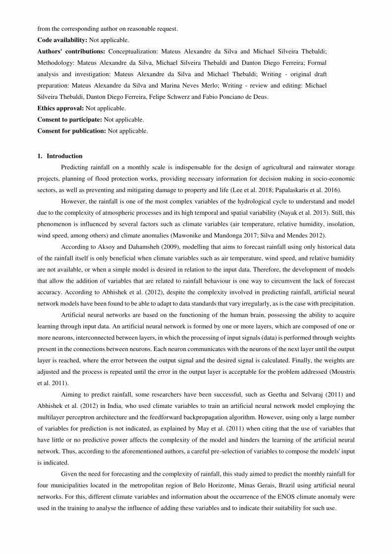
Table 1 Identification and characteristics of the municipalities covered in the study.
Climatological station (city)
Latitude Longitude Köppen climate classification -
(Martins et al. 2018)
Altitude (m)
Average annual rainfall
(mm)*
Belo Horizonte -19.934382 -43.952292 Aw 915.17 1544.64
C. do Mato Dentro -19.020355 -43.433948 Aw 663.02 1283.50
Florestal -19.885422 -44.416889 Cwa 753.51 1399.29 Sete Lagoas -19.48454 -44.173798 Aw 753.68 1325.69
* = Referring to the period of the training data (1970 – 1999). Aw = tropical with winter drought. Cwa = subtropical with dry winter and hot summer.
The Figure 1 shows the geographical location of the municipalities covered in the study.
Fig. 1 Geographic location of the municipalities covered in the study.
The criterion for the choice of the mesoregion was the existence of at least 4 stations with monthly data of total
precipitation, mean compensated temperature, mean relative humidity and mean wind speed in the period between the
years 1970 and 2009. The following criteria were established for the choice of climatological stations: being part of the
same mesoregion, having a maximum altitude difference of 300 m between them and presenting, considering the historical
series of all the variables mentioned above, the maximum percentage of failure of 30%.
2.2. Obtaining the data used in the training and the validation of the artificial neural networks
The sequence number corresponding to the month (1 to 12) was used to compose the database for training and
validation of artificial neural networks, in addition to the historical monthly total of precipitation, average compensated
temperature, average relative humidity and average wind speed for the years 1970 to 2009, obtained from the BDMEP
platform - Database of the National Institute of Meteorology (Instituto Nacional de Meteorologia - INMET 2020).
To provide data on the occurrence of the climate phenomena El Niño and La Niña, was used the Multivariate
ENSO Index (MEI) for the years 1970 to 2009, with bimonthly records, obtained from the National Oceanic and
Atmospheric Administration platform (National Oceanic and Atmospheric Administration - NOAA 2020). In this case,
the lowest value (1) indicates stronger cases of La Niña, while the highest value (69) indicates stronger cases of El Niño.
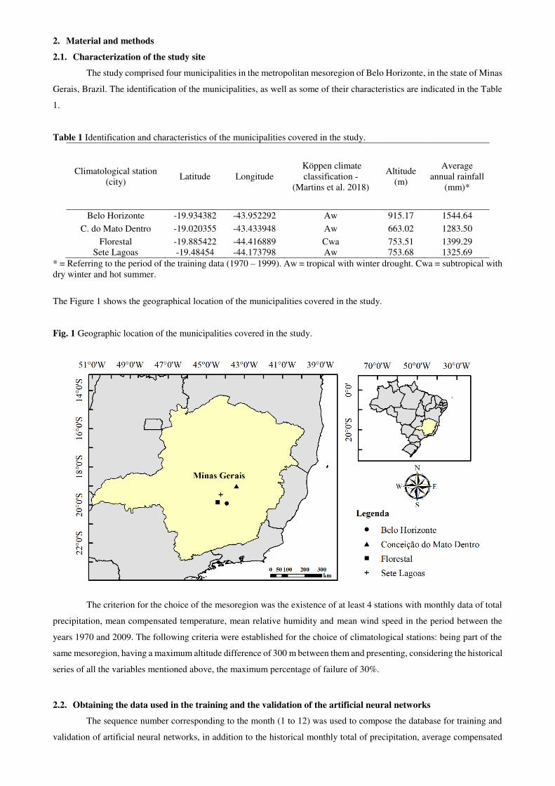
The average monthly precipitation values at the climatological stations covered in this study, calculated using
the months without failures, for the period from 1970 to 2009, are presented in Figure 2.
Fig. 2 Average monthly rainfall, in millimeters (mm), observed at the climatological stations discussed in this study.
Obs
erve
d ra
infa
ll (m
m)
0
200
400
600
800
1970
1980
1990
2000
2010
2.3. Data preprocessing
To achieve a single monthly value for the MEI, a weighted average between the overlapping months (December
- January; January - February; (...); November - December) was conducted using as basis the number of days in each
month.
The database was divided into two intervals: training (1970 - 1999) and validation (2000 - 2009), the latter being
variable due to the availability of data from each climatological station. In order to ensure that the characteristics of the
historical series did not change, no procedure for gap filling was conducted.
In order to verify the hydrological homogeneity of the region where the climatological stations are located, as
well as the consistency of monthly rainfall data for the training period, the double mass curve was used as described in
Agência Nacional das Águas - ANA (2012). This verification was performed so that the monthly rainfall observed at each
of the stations was validated (ordinate axis), while the average of the other stations was considered as the reference
observed monthly rainfall (abscissa axis).
In order to verify the existence of a tendency in the historical series of total monthly rainfall for the training
period (1970 to 1999), the Mann-Kendall test performed was admitting a significance level of 5% (p-value < 0.05).
For the network training, rainfall at time "t+1" and three combinations of input data were set as targets:
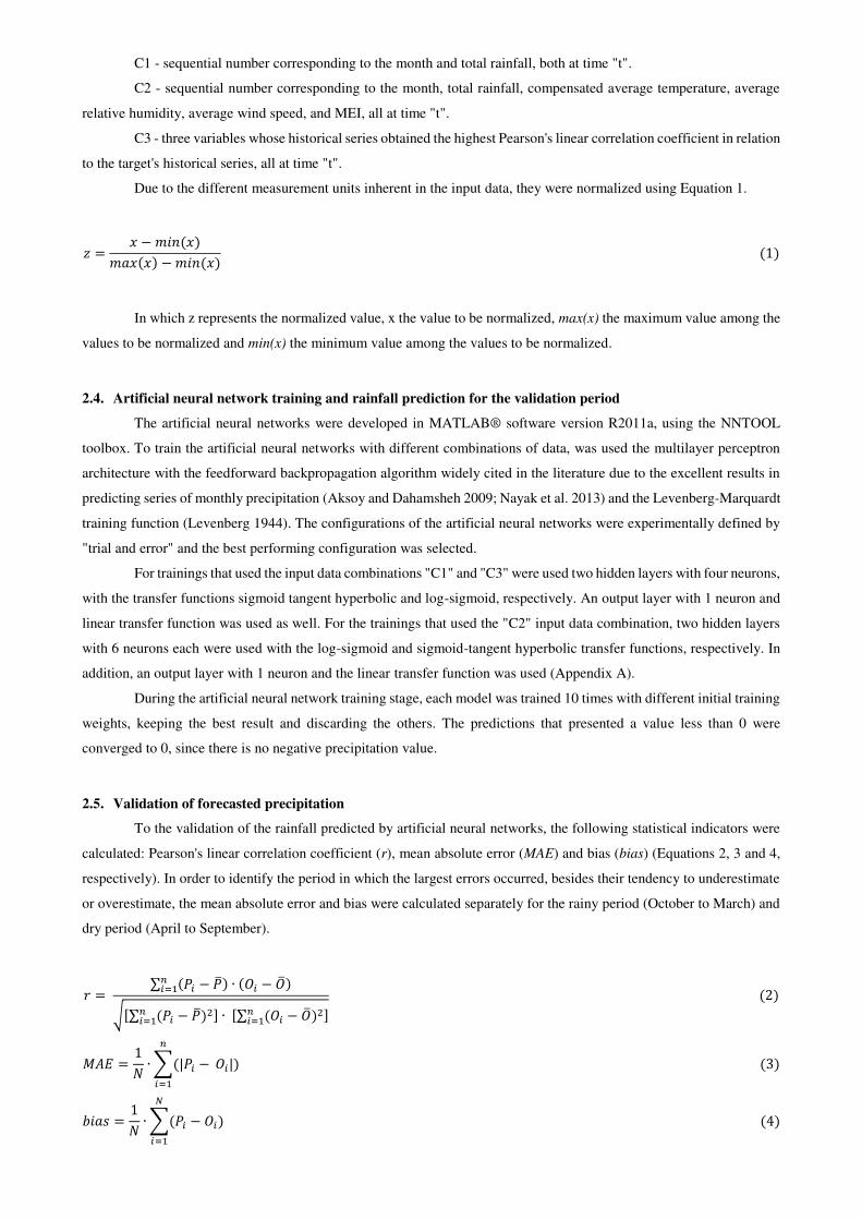
C1 - sequential number corresponding to the month and total rainfall, both at time "t".
C2 - sequential number corresponding to the month, total rainfall, compensated average temperature, average
relative humidity, average wind speed, and MEI, all at time "t".
C3 - three variables whose historical series obtained the highest Pearson's linear correlation coefficient in relation
to the target's historical series, all at time "t".
Due to the different measurement units inherent in the input data, they were normalized using Equation 1.
𝑧 = 𝑥 − 𝑚𝑖𝑛(𝑥)𝑚𝑎𝑥(𝑥) − 𝑚𝑖𝑛(𝑥) (1)
In which z represents the normalized value, x the value to be normalized, max(x) the maximum value among the
values to be normalized and min(x) the minimum value among the values to be normalized.
2.4. Artificial neural network training and rainfall prediction for the validation period
The artificial neural networks were developed in MATLAB® software version R2011a, using the NNTOOL
toolbox. To train the artificial neural networks with different combinations of data, was used the multilayer perceptron
architecture with the feedforward backpropagation algorithm widely cited in the literature due to the excellent results in
predicting series of monthly precipitation (Aksoy and Dahamsheh 2009; Nayak et al. 2013) and the Levenberg-Marquardt
training function (Levenberg 1944). The configurations of the artificial neural networks were experimentally defined by
"trial and error" and the best performing configuration was selected.
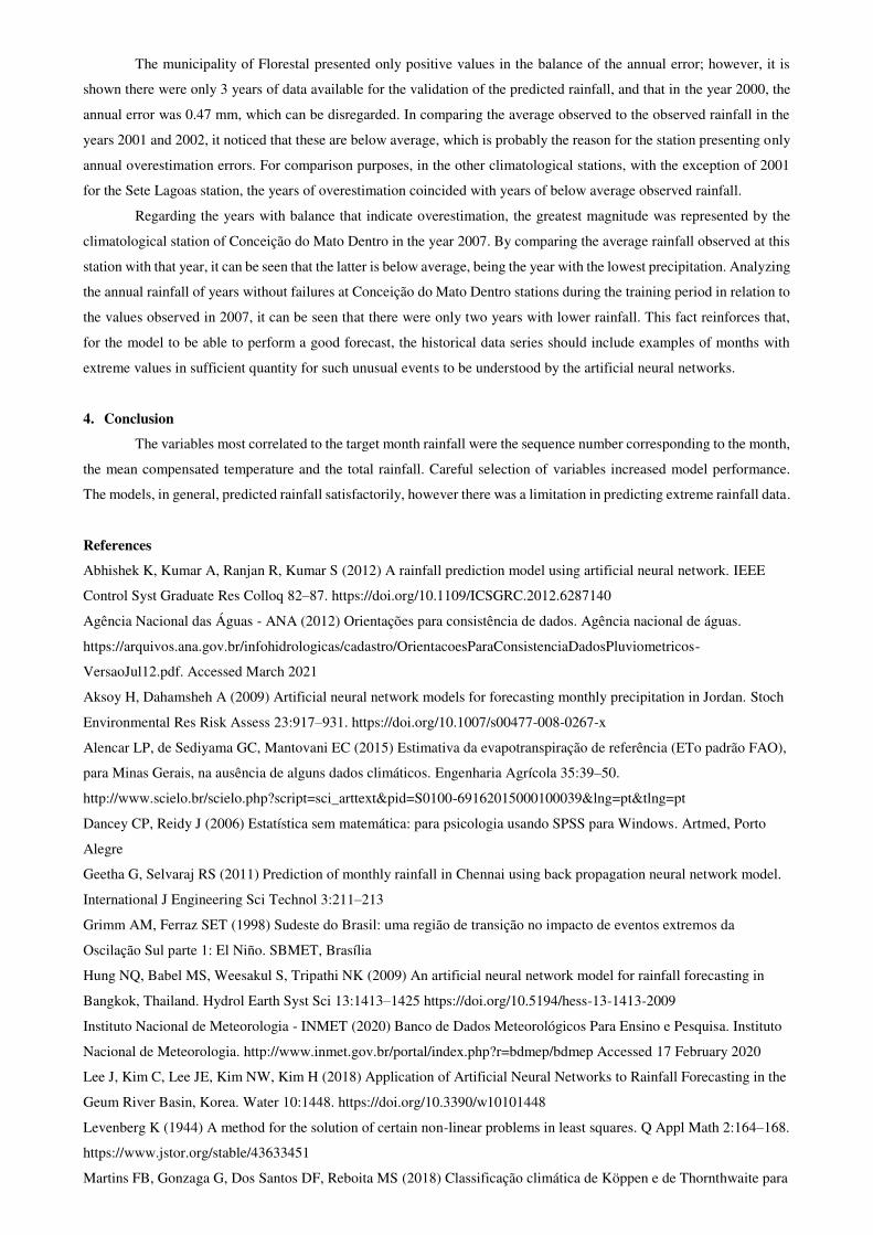
For trainings that used the input data combinations "C1" and "C3" were used two hidden layers with four neurons,
with the transfer functions sigmoid tangent hyperbolic and log-sigmoid, respectively. An output layer with 1 neuron and
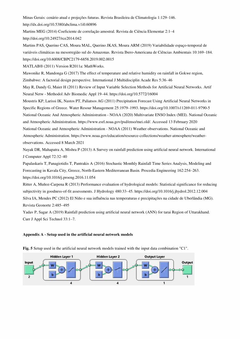
linear transfer function was used as well. For the trainings that used the "C2" input data combination, two hidden layers
with 6 neurons each were used with the log-sigmoid and sigmoid-tangent hyperbolic transfer functions, respectively. In
addition, an output layer with 1 neuron and the linear transfer function was used (Appendix A).
During the artificial neural network training stage, each model was trained 10 times with different initial training
weights, keeping the best result and discarding the others. The predictions that presented a value less than 0 were
converged to 0, since there is no negative precipitation value.
2.5. Validation of forecasted precipitation
To the validation of the rainfall predicted by artificial neural networks, the following statistical indicators were
calculated: Pearson's linear correlation coefficient (r), mean absolute error (MAE) and bias (bias) (Equations 2, 3 and 4,
respectively). In order to identify the period in which the largest errors occurred, besides their tendency to underestimate
or overestimate, the mean absolute error and bias were calculated separately for the rainy period (October to March) and
dry period (April to September).
𝑟 = ∑ (𝑃𝑖 − �̅�) ∙ (𝑂𝑖 − �̅�)𝑛𝑖=1√[∑ (𝑃𝑖 − �̅�)2𝑛𝑖=1 ] ∙ [∑ (𝑂𝑖 − �̅�)2𝑛𝑖=1 ] (2)
𝑀𝐴𝐸 = 1𝑁 ∙ ∑(|𝑃𝑖 −𝑛𝑖=1 𝑂𝑖|) (3)
𝑏𝑖𝑎𝑠 = 1𝑁 ∙ ∑(𝑃𝑖𝑁𝑖=1 − 𝑂𝑖) (4)

In which "O" represents the observed data at the climatological stations, “�̅�” the average of the observed data,
"P" the data predicted by the artificial neural networks, and "N" the amount of data for validation. The values of "N"
varied with the availability of data from each climatological station in the validation period, for the municipalities of Belo
Horizonte, Conceição do Mato Dentro, Florestal, and Sete Lagoas, respectively, for data combination "C1", 120, 199,
109, and 120, for data combination "C2" and "C3", 120, 118, 29, and 120.
When it comes to Pearson's linear correlation coefficient, according to Dancey and Reidy (2006), it is possible
to classify the degree of correlation between two variables into three classes: weak correlation of 0.10 < r < 0.30; moderate
of 0.40 < r < 0.60; and strong of 0.70 < r < 1.00.
To evaluate the model performance, the 𝑛𝑡 index (Equation 5) proposed by Ritter and Muñoz-Carpena (2013)
was used. The 𝑛𝑡 index suggests that model efficiency should be considered satisfactory when the error is "small", taking
into account the width of the data range covered by the calculated values. This index ensures that a model that predicts
precipitation with a small error value within a small data range is not considered better than another model that predicts
with a larger error value, but within a larger data range.
In this way, the efficiency of the model is evaluated depending on the number of times (𝑛𝑡) that the variability
of the observations is greater than the mean error of the model. To this end, the mean error is represented by the square
root of the root mean square error (RMSE) and the variability of the observed data by the population standard deviation
(SD).
𝑛𝑡 = 𝑆𝐷𝑅𝑀𝑆𝐸 − 1 (5)
Ritter and Muñoz-Carpena (2013) also defined four performance classes based on the 𝑛𝑡 index, with 𝑛𝑡 < 0.7
unsatisfactory, 0.7 ≤ 𝑛𝑡 < 1.2 acceptable, 1.2 ≤ 𝑛𝑡 < 2.2 good and 2.2 ≤ 𝑛𝑡 very good.
In order to verify possible significant differences between the observed and predicted historical series for the
best performing combination, the Mann-Whitney test was performed, assuming a significance level of 5% (p-value <
0.05).
In addition, the magnitude of the error on an annual scale was calculated by subtracting the value of the observed
annual rainfall from the value of the predicted rainfall.
3. Results and Discussion
3.1. Characterization of monthly precipitation data
The hydrological homogeneity of the region where the climatological stations are inserted, as well as the
consistency of the data from the historical series of monthly precipitation were proven by the high values of the
determination coefficients (R² = 0.9976 - 0.9995), obtained by fitting the linear trend line to the double mass curve. Thus,
it can be affirmed that the hydrological behavior in the climatological stations is similar, as well as eliminate the
occurrence of errors of transcription of the data observed in the field or alteration of the angular coefficient of the straight
line.
The Table 2 shows the p-values and "τ" obtained by applying the Mann-Kendall test, at 5% significance level,
to the historical series of total monthly precipitation of the climatological stations addressed in this study, during the
training period.
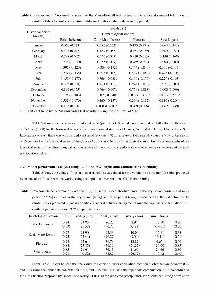
Table 2 p-values and "τ" obtained by means of the Mann-Kendall test applied to the historical series of total monthly
rainfall of the climatological stations addressed in this study, in the training period.
Historical Series (month)
p-value (τ) Climatological stations
Belo Horizonte C. do Mato Dentro Florestal Sete Lagoas
January 0.066 (0.223) 0.196 (0.152) 0.133 (0.174) 0.064 (0.241)
February 0.443 (0.092) 0.657 (0.055) 0.454 (0.089) 0.669 (0.057)
March 0.798 (0.032) 0.766 (0.037) 0.910 (0.015) 0.199 (0.168)
April 0.744 (-0.040) 0.755 (0.039) 0.989 (0.003) 1.000 (0.002)
May 0.306 (-0.123) 0.109 (-0.192) 0.744 (-0.040) 0.301 (-0.136)
June 0.274 (-0.135) 0.926 (0.013) 0.527 (-0.080) 0.427 (-0.108)
July 0.155 (-0.177) 0.766 (-0.038) 0.160 (-0.179) 0.229 (-0.163)
August 0.382 (0.108) 0.431 (0.098) 0.945 (-0.010) 0.971 (0.007)
September 0.196 (0.155) 0.966 (-0.007) 0.754 (-0.038) 1.000 (0.000)
October 0.125 (-0.183) 0.002 (-0.378)* 0.007 (-0.317)* 0.019 (-0.299)*
November 0.532 (-0.076) 0.260 (-0.137) 0.264 (-0.132) 0.110 (-0.204)
December 0.132 (0.180) 0.001 (0.401)* 0.969 (0.006) 0.062 (0.239)
* = significant trend by the Mann-Kendall test admitting a significance level of 5%.
Table 2 shows that there was a significant trend (p-value < 0.05) of decrease in total rainfall values in the month
of October (τ < 0) for the historical series of the climatological stations of Conceição do Mato Dentro, Florestal and Sete
Lagoas. In contrast, there was only a significant trend (p-value > 0) of increase in total rainfall values (τ > 0) for the month
of December for the historical series of the Conceição do Mato Dentro climatological station. For the other months of the
historical series of the climatological stations analyzed, there was no significant trend of increase or decrease of the total
precipitation value.
3.2. Model performance analysis using "C1" and "C2" input data combinations in training
Table 3 shows the values of the statistical indicators calculated for the validation of the rainfall series predicted
by means of artificial neural networks, using the input data combination "C1" in the training.
Table 3 Pearson's linear correlation coefficient (r), 𝑛𝑡 index, mean absolute error in the dry period (MAEd) and rainy
period (MAEr) and bias in the dry period (biasd) and rainy period (biasr), calculated for the validation of the
rainfall series predicted by means of artificial neural networks using for training the input data combination "C1"
(without parentheses) and "C2" (in parentheses).
Climatological station 𝑟 𝑀𝐴𝐸𝑑 (mm) 𝑀𝐴𝐸𝑟 (mm) 𝑏𝑖𝑎𝑠𝑑 (mm) 𝑏𝑖𝑎𝑠𝑟 (mm) 𝑛𝑡
Belo Horizonte 0.84
(0.83) 23.85
(25.57) 86.23
(90.75) 2.94
(-3.28) -23.50
(-14.61) 0.80
(0.80)
C. do Mato Dentro 0.77
(0.75) 25.90
(25.44) 92.33
(96.27) 10.04 (9.34)
-17.81 (-3.11)
0.55 (0.51)
Florestal 0.78
(0.84) 23.64
(23.85) 76.79
(56.10) 13.87
(21.32) 4.65
(-31.00) 0.60
(0.83)
Sete Lagoas 0.85
(0.78) 21.64
(40.52) 76.43
(72.87) 11.66
(26.37) -24.66
(-17.12) 0.80
(0.60)
From Table 3 it can be seen that the values of Pearson's linear correlation coefficient obtained are between 0.77
and 0.85 using the input data combination "C1", and 0.75 and 0.84 using the input data combination "C2". According to
the classification proposed by Dancey and Reidy (2006), all the predicted precipitation series obtained strong correlation
with the observed rainfall series. Such classification indicates linearity between the increase in values of the observed and
predicted series, suggesting that if the observed data are above average, the predicted will also be (Martins 2014). Thus,
it is noted that the models were able to successfully predict the seasonality present in the historical series of data,
identifying the months with higher and lower rainfall rates.
However, it can be seen that, with the exception of the climatological station in the Florestal municipality, the
correlation values obtained using the "C2" input data combination decreased in relation to the values obtained for training
the artificial neural networks using the "C1" input data combination.
The values of the mean absolute error for the dry period were between 21.64 and 25.90 mm using the "C1" data
combination and 23.85 and 40.52 mm using the "C2" data combination, with the highest values obtained using the "C2"
input data combination. Comparing the values of the mean absolute error to the mean of the dry period precipitation, these
can be regarded as high, but there is a sharp reduction in the value of the mean, caused by the months with low or no
precipitation. Thus, the errors of the dry period are less relevant if compared to the rainfall values of each month of the
dry period.
Analyzing also the dry period bias it is noted that the values were between 2.94 and 13.87 mm using the input
data combination "C1" and -3.28 and 26.37 mm using the input data combination "C2". That shows, with the exception
of the model developed for the Belo Horizonte climatological station using the "C2" input data set, that the models
overestimated precipitation, reinforcing the idea that the values obtained for the mean absolute error for the dry period
were influenced by the drier months of the dry period. Furthermore, the highest bias values achieved were using the "C2"
input data combination.
The mean absolute error values for the wet season were in the range of 76.43 to 92.33 mm using the "C1" input
data combination and 56.10 to 96.27 mm using the "C2" input data combination, high values even for the wettest months.
For the bias of this same period, it is observed that, the values comprised between -24.66 and 4.65 mm using the
combination and input data "C1" and -31.00 and -3.11 mm using the combination of input data "C2". Among these values,
there was only one positive value, obtained for the climatological station in the municipality of Florestal when using the
combination of input data "C1" in training the artificial neural networks.
This fact indicates that the models underestimated the rainy season precipitation, and the lack of accuracy of the
artificial neural networks in predicting the wettest months is a possible factor for the increased error and bias. Although
the mean absolute error values for the rainy period obtained using the combination of input data "C2" indicates, in most
stations, a reduction when compared to "C1", except for Florestal, this reduction was not significant.
The values of the index 𝑛𝑡 using the input data combination "C1" were between 0.55 and 0.80. For the
climatological stations in the Conceição do Mato Dentro and Florestal municipalities, the model was classified as
unsatisfactory and for the climatological stations in the Belo Horizonte and Sete Lagoas municipalities, classified as
acceptable (Ritter and Muñoz-Carpena 2013). Using the combination of input data "C2", the values of the index 𝑛𝑡 were
between 0.51 and 0.83. For the climatological stations in the Conceição do Mato Dentro and Sete Lagoas municipalities,
the model was classified as unsatisfactory and for the climatological stations in the Belo Horizonte and Florestal
municipalities, acceptable (Ritter and Muñoz-Carpena 2013).
Similar to the result obtained by Pearson's linear correlation coefficient, the 𝑛𝑡 index indicated a regression in
the model performance of the climatological stations of Conceição do Mato Dentro and Sete Lagoas using the combination
of input data "C2" in relation to the use of the combination of input data "C1" for training the artificial neural networks.
For the climate stations in the municipalities of Florestal and Belo Horizonte there was an increase and constancy of the
index, respectively.
Through the joint analysis of the results, it is noted, in general, that the addition of the climatological variables
impaired the performance of the models. Although the component variables of the "C2" input data combination are used
by meteorologists to feed models that predict the climate and its variability (NOAA 2011), they can present changes in
their behavior in short periods of time, being more useful for forecasting on a smaller temporal scale, such as the hourly
and daily scale.
As an example, Martins et al. (2019) explain in their study that the relative humidity reaches higher percentages
at night. Thus, on scales larger than the hourly, such as the monthly scale, these values are reduced because they are
measured as the average of the period.
Such behavior of the models can also be explained from what is exposed by May et al. (2011). The authors
present that the models of artificial neural networks can go through problems of under-specification due to the choice of
insufficient or uninformative input variables, or even by over-specification due to the use of uninformative, uninformative
or even redundant variables. These problems can affect model complexity, learning difficulty, and artificial neural
network performance. The authors add that to train a neural network, it is necessary to select the input variables and one
of the widely used methods is to classify the variable based on Pearson correlation, performing the selection in descending
order of classification.
3.3. Variable selection for training artificial neural network models
In order to select the variables most correlated to precipitation to compose input data combination "C3", Table
4 shows the Pearson's linear correlation coefficient values obtained between the input variables used in input data
combination "C2" and the target.
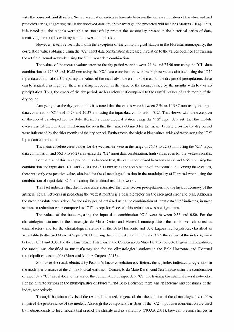
Table 4 Pearson's linear correlation coefficient calculated between the variables sequence number corresponding to the
month (N), total precipitation (P), average compensated temperature (T), average relative humidity (H), average
wind speed (W) and MEI, and the target for the choice of variables for the input data combination "C3".
Climatological station N P T H W MEI Belo Horizonte 0.33 0.47 0.45 0.21 0.12 0.03
C. do Mato Dentro 0.38 0.44 0.49 -0.08 0.37 0.01 Florestal 0.38 0.43 0.51 0.09 0.08 0.04
Sete Lagoas 0.39 0.47 0.48 0.17 0.26 0.01
Average 0.37 0.45 0.48 0.10 0.21 0.02
Through Table 4, it is possible to verify that both for the average and individually the three variables that obtained
higher values for Pearson's linear correlation coefficient were mean compensated temperature, total precipitation and
number corresponding to the month, respectively. In contrast, the average relative humidity, wind speed and the MEI, in
general, had small correlation values.
It is known that wet air favors the formation of rainfall, as in the occurrence of convective precipitation and that
wind speed affects the behavior of evapotranspiration. However, in this study, these variables do not have great predictive
power for the rainfall of the following month.
Regarding relative humidity, the result obtained does not corroborate with the one presented by Hung et al.
(2009) who, with the objective of predicting rainfall one hour ahead in Bangkok, Thailand, using the generalized
feedforward architecture, found that relative humidity was directly linked to good model performance. Mawonike and
Mandonga (2017), who present that variability in relative humidity affects the occurrence of precipitation, but the
maximization of this effect happens when relative humidity is above 80%, can explain the divergence between results.
These values are observed less frequently on a monthly scale, since days with low values of relative humidity reduce the
average values.
As for the wind speed variable, the possible explanation for the low correlation, according to Alencar et al.
(2015), is that the variation of the average wind speed in monthly periods is relatively low, i.e., while there is a large
discrepancy between the monthly precipitation values the monthly wind speed values remain with a small variability.
The lowest Pearson's linear correlation coefficient corresponds to the MEI. This fact can be explained, according
to Grimm and Ferraz (1998), by the Southeast region of Brazil, where the study area is inserted, has a transitional
character. Thus, the anomalies (El Niño and La Niña) can move more to the North or South from one event to another,
making it possible to change the effects in relation to the same event that occurred previously, which does not occur for
the extreme South of Brazil.
Thus, for the input data combination "C3", the three variables that obtained the highest value of Pearson's linear
correlation coefficient with the target were used, i.e., number corresponding to the month, average compensated
temperature, and total precipitation.
3.4. Analysis of model performance using the "C3" input data combination in training
The statistical indicators for the validation of the forecasted rainfall series using in the training of the artificial
neural networks the input data combination "C3" are arranged in Table 5.
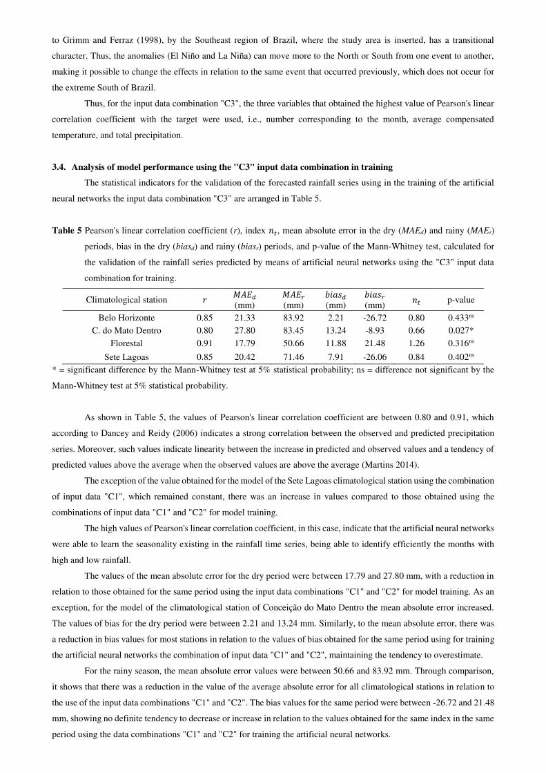
Table 5 Pearson's linear correlation coefficient (r), index 𝑛𝑡, mean absolute error in the dry (MAEd) and rainy (MAEr)
periods, bias in the dry (biasd) and rainy (biasr) periods, and p-value of the Mann-Whitney test, calculated for
the validation of the rainfall series predicted by means of artificial neural networks using the "C3" input data
combination for training.
Climatological station 𝑟 𝑀𝐴𝐸𝑑
(mm) 𝑀𝐴𝐸𝑟 (mm)
𝑏𝑖𝑎𝑠𝑑
(mm) 𝑏𝑖𝑎𝑠𝑟
(mm) 𝑛𝑡 p-value
Belo Horizonte 0.85 21.33 83.92 2.21 -26.72 0.80 0.433ns
C. do Mato Dentro 0.80 27.80 83.45 13.24 -8.93 0.66 0.027*
Florestal 0.91 17.79 50.66 11.88 21.48 1.26 0.316ns
Sete Lagoas 0.85 20.42 71.46 7.91 -26.06 0.84 0.402ns
* = significant difference by the Mann-Whitney test at 5% statistical probability; ns = difference not significant by the
Mann-Whitney test at 5% statistical probability.
As shown in Table 5, the values of Pearson's linear correlation coefficient are between 0.80 and 0.91, which
according to Dancey and Reidy (2006) indicates a strong correlation between the observed and predicted precipitation
series. Moreover, such values indicate linearity between the increase in predicted and observed values and a tendency of
predicted values above the average when the observed values are above the average (Martins 2014).
The exception of the value obtained for the model of the Sete Lagoas climatological station using the combination
of input data "C1", which remained constant, there was an increase in values compared to those obtained using the
combinations of input data "C1" and "C2" for model training.
The high values of Pearson's linear correlation coefficient, in this case, indicate that the artificial neural networks
were able to learn the seasonality existing in the rainfall time series, being able to identify efficiently the months with
high and low rainfall.
The values of the mean absolute error for the dry period were between 17.79 and 27.80 mm, with a reduction in
relation to those obtained for the same period using the input data combinations "C1" and "C2" for model training. As an
exception, for the model of the climatological station of Conceição do Mato Dentro the mean absolute error increased.
The values of bias for the dry period were between 2.21 and 13.24 mm. Similarly, to the mean absolute error, there was
a reduction in bias values for most stations in relation to the values of bias obtained for the same period using for training
the artificial neural networks the combination of input data "C1" and "C2", maintaining the tendency to overestimate.
For the rainy season, the mean absolute error values were between 50.66 and 83.92 mm. Through comparison,
it shows that there was a reduction in the value of the average absolute error for all climatological stations in relation to
the use of the input data combinations "C1" and "C2". The bias values for the same period were between -26.72 and 21.48
mm, showing no definite tendency to decrease or increase in relation to the values obtained for the same index in the same
period using the data combinations "C1" and "C2" for training the artificial neural networks.
Using the combination of input data "C3" in training the artificial neural networks, the index 𝑛𝑡 presented values
between 0.66 and 1.26. Thus, the model was rated as unsatisfactory for the climatological station in the municipality of
Conceição do Mato Dentro, acceptable for the climatological stations in the municipalities of Belo Horizonte and Sete
Lagoas, and good for the climatological station in the municipality of Florestal. It shows that the values of the index 𝑛𝑡
increased for all climatological stations in relation to the values obtained for training the artificial neural networks
performed with the combinations of input data "C1" and "C2". Using the "C3" combination of input data for training,
there were fewer models rated as unsatisfactory compared to the other combinations, and one model rated as good, which
had not occurred before.
Comparing the results obtained using different combinations of input data for training the artificial neural
networks, it can be seen that the model performance using only the three variables that obtained higher correlation
coefficients with the target (input data combination "C3") for training the neural networks improved. Similarly, Lee et al.
(2018) using the multilayer perceptron architecture in addition to the feedfoward backpropagation algorithm, attempted
to predict rainfall in South Korea by initially using data from 10 different climate indices. After an evaluation and selection
of five indices that showed better results, the authors obtained a better model performance.
Furthermore, according to the Mann-Whitney test, only for the climatological station of the Conceição do Mato
Dentro municipality there was a significant difference between the observed and predicted series. This can be explained
by the greater magnitude of the mean absolute error value for the dry period obtained for the model of the climatological
station of Conceição do Mato Dentro municipality, this value being about 40% higher than the average of the values
obtained for the other climatological stations. Such an increase in values causes the median of the predicted precipitation
series to also increase, becoming statistically significant.
For the other climatological stations, there was not enough evidence to conclude that there was a significant
difference between observed and predicted series, that is, no discrepant differences were detected between the median
value of the observed and estimated series. This indicates a satisfactory performance of the models; because the fact that
there is no statistically significant difference between the median values, coupled with the high values of Pearson's linear
correlation coefficient, means that, the predicted series reproduced the seasonality inherent in the observed rainfall series.
Aiming at a visual analysis of the results obtained for training the artificial neural networks using the "C3" input
data combination, the precipitation values observed and predicted by the artificial neural networks on a monthly scale
were plotted in Figure 3.
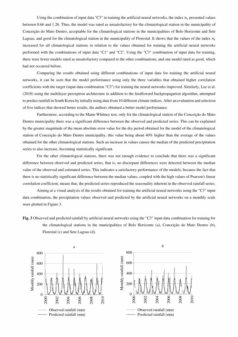
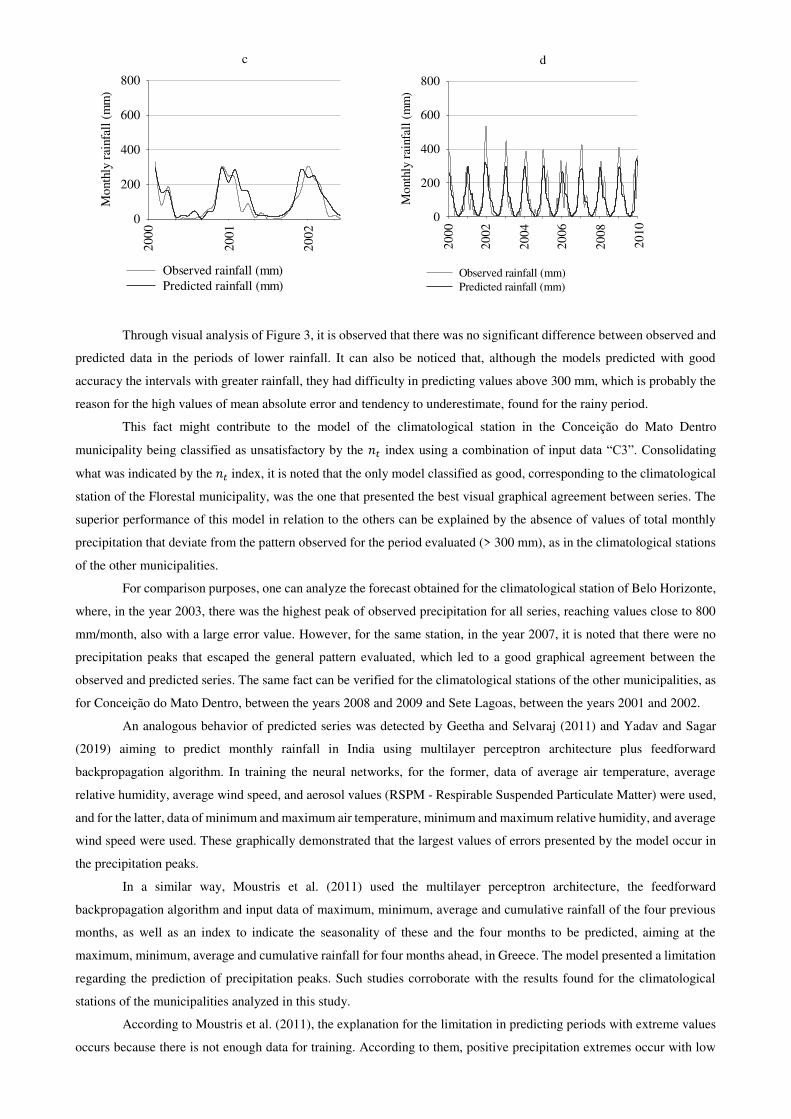
Fig. 3 Observed and predicted rainfall by artificial neural networks using the "C3" input data combination for training for
the climatological stations in the municipalities of Belo Horizonte (a), Conceição do Mato Dentro (b),
Florestal (c) and Sete Lagoas (d).
a
Mon
thly
rai
nfal
l (m
m)
0
200
400
600
800
Observed rainfall (mm) Predicted rainfall (mm)
2000
2002
2004
2006
2008
2010
b
Mon
thly
rai
nfal
l (m
m)
Observed rainfall (mm)Predicted rainfall (mm)
2000
2002
2004
2006
2008
2010
0
200
400
600
800
c
Mon
thly
rai
nfal
l (m
m)
0
200
400
600
800
Observed rainfall (mm)Predicted rainfall (mm)
2000
2001
2002
d
Mon
thly
rai
nfal
l (m
m)
0
200
400
600
800
Observed rainfall (mm)Predicted rainfall (mm)
2000
2002
2004
2006
2008
2010
Through visual analysis of Figure 3, it is observed that there was no significant difference between observed and
predicted data in the periods of lower rainfall. It can also be noticed that, although the models predicted with good
accuracy the intervals with greater rainfall, they had difficulty in predicting values above 300 mm, which is probably the
reason for the high values of mean absolute error and tendency to underestimate, found for the rainy period.
This fact might contribute to the model of the climatological station in the Conceição do Mato Dentro
municipality being classified as unsatisfactory by the 𝑛𝑡 index using a combination of input data “C3”. Consolidating
what was indicated by the 𝑛𝑡 index, it is noted that the only model classified as good, corresponding to the climatological
station of the Florestal municipality, was the one that presented the best visual graphical agreement between series. The
superior performance of this model in relation to the others can be explained by the absence of values of total monthly
precipitation that deviate from the pattern observed for the period evaluated (> 300 mm), as in the climatological stations
of the other municipalities.
For comparison purposes, one can analyze the forecast obtained for the climatological station of Belo Horizonte,
where, in the year 2003, there was the highest peak of observed precipitation for all series, reaching values close to 800
mm/month, also with a large error value. However, for the same station, in the year 2007, it is noted that there were no
precipitation peaks that escaped the general pattern evaluated, which led to a good graphical agreement between the
observed and predicted series. The same fact can be verified for the climatological stations of the other municipalities, as
for Conceição do Mato Dentro, between the years 2008 and 2009 and Sete Lagoas, between the years 2001 and 2002.
An analogous behavior of predicted series was detected by Geetha and Selvaraj (2011) and Yadav and Sagar
(2019) aiming to predict monthly rainfall in India using multilayer perceptron architecture plus feedforward
backpropagation algorithm. In training the neural networks, for the former, data of average air temperature, average
relative humidity, average wind speed, and aerosol values (RSPM - Respirable Suspended Particulate Matter) were used,
and for the latter, data of minimum and maximum air temperature, minimum and maximum relative humidity, and average
wind speed were used. These graphically demonstrated that the largest values of errors presented by the model occur in
the precipitation peaks.
In a similar way, Moustris et al. (2011) used the multilayer perceptron architecture, the feedforward
backpropagation algorithm and input data of maximum, minimum, average and cumulative rainfall of the four previous
months, as well as an index to indicate the seasonality of these and the four months to be predicted, aiming at the
maximum, minimum, average and cumulative rainfall for four months ahead, in Greece. The model presented a limitation
regarding the prediction of precipitation peaks. Such studies corroborate with the results found for the climatological
stations of the municipalities analyzed in this study.
According to Moustris et al. (2011), the explanation for the limitation in predicting periods with extreme values
occurs because there is not enough data for training. According to them, positive precipitation extremes occur with low
frequency and high randomness, and if there are not enough records in the data used for training the artificial neural
networks, they will not acquire the necessary experience for prediction.
It shows that the climatological station in the Conceição do Mato Dentro municipality there was a tendency to
increase the error values for the rainy period over the years used in the validation. This can be explained by the tendency
of increase in precipitation values found for the historical series of December of the climatological station of Conceição
do Mato Dentro using the Mann-Kendall test (Table 2), thus aggravating the precipitation peaks of the rainy season.
The balance of the error on an annual scale between the precipitation predicted by means of artificial neural
networks using the combination of input data "C3" in training and observed for the climatological stations of the
municipalities analyzed in the study is indicated in Figure 4.
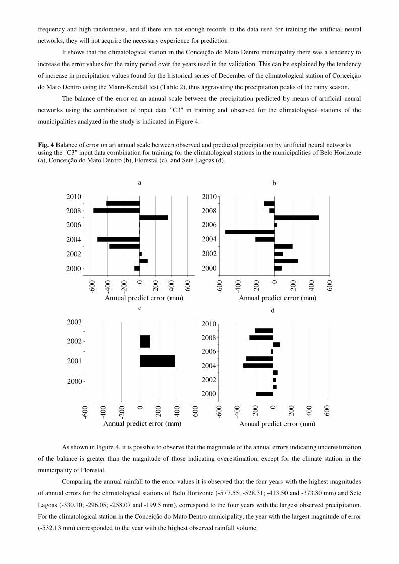
Fig. 4 Balance of error on an annual scale between observed and predicted precipitation by artificial neural networks using the "C3" input data combination for training for the climatological stations in the municipalities of Belo Horizonte (a), Conceição do Mato Dentro (b), Florestal (c), and Sete Lagoas (d).
a
Annual predict error (mm)
-600
-400
-200 0
200
400
600
2000
2002
2004
2006
2008
2010
b
Annual predict error (mm)
-600
-400
-200 0
200
400
600
2000
2002
2004
2006
2008
2010
c
Annual predict error (mm)
-600
-400
-200 0
200
400
600
2000
2001
2002
2003
d
Annual predict error (mm)
2000
2002
2004
2006
2008
2010
0
200
400
600
-200
-400
-600
As shown in Figure 4, it is possible to observe that the magnitude of the annual errors indicating underestimation
of the balance is greater than the magnitude of those indicating overestimation, except for the climate station in the
municipality of Florestal.
Comparing the annual rainfall to the error values it is observed that the four years with the highest magnitudes
of annual errors for the climatological stations of Belo Horizonte (-577.55; -528.31; -413.50 and -373.80 mm) and Sete
Lagoas (-330.10; -296.05; -258.07 and -199.5 mm), correspond to the four years with the largest observed precipitation.
For the climatological station in the Conceição do Mato Dentro municipality, the year with the largest magnitude of error
(-532.13 mm) corresponded to the year with the highest observed rainfall volume.
The municipality of Florestal presented only positive values in the balance of the annual error; however, it is
shown there were only 3 years of data available for the validation of the predicted rainfall, and that in the year 2000, the
annual error was 0.47 mm, which can be disregarded. In comparing the average observed to the observed rainfall in the
years 2001 and 2002, it noticed that these are below average, which is probably the reason for the station presenting only
annual overestimation errors. For comparison purposes, in the other climatological stations, with the exception of 2001
for the Sete Lagoas station, the years of overestimation coincided with years of below average observed rainfall.
Regarding the years with balance that indicate overestimation, the greatest magnitude was represented by the
climatological station of Conceição do Mato Dentro in the year 2007. By comparing the average rainfall observed at this
station with that year, it can be seen that the latter is below average, being the year with the lowest precipitation. Analyzing
the annual rainfall of years without failures at Conceição do Mato Dentro stations during the training period in relation to
the values observed in 2007, it can be seen that there were only two years with lower rainfall. This fact reinforces that,
for the model to be able to perform a good forecast, the historical data series should include examples of months with
extreme values in sufficient quantity for such unusual events to be understood by the artificial neural networks.
4. Conclusion
The variables most correlated to the target month rainfall were the sequence number corresponding to the month,
the mean compensated temperature and the total rainfall. Careful selection of variables increased model performance.
The models, in general, predicted rainfall satisfactorily, however there was a limitation in predicting extreme rainfall data.
References
Abhishek K, Kumar A, Ranjan R, Kumar S (2012) A rainfall prediction model using artificial neural network. IEEE
Control Syst Graduate Res Colloq 82–87. https://doi.org/10.1109/ICSGRC.2012.6287140
Agência Nacional das Águas - ANA (2012) Orientações para consistência de dados. Agência nacional de águas.
https://arquivos.ana.gov.br/infohidrologicas/cadastro/OrientacoesParaConsistenciaDadosPluviometricos-
VersaoJul12.pdf. Accessed March 2021
Aksoy H, Dahamsheh A (2009) Artificial neural network models for forecasting monthly precipitation in Jordan. Stoch
Environmental Res Risk Assess 23:917–931. https://doi.org/10.1007/s00477-008-0267-x
Alencar LP, de Sediyama GC, Mantovani EC (2015) Estimativa da evapotranspiração de referência (ETo padrão FAO),
para Minas Gerais, na ausência de alguns dados climáticos. Engenharia Agrícola 35:39–50.
http://www.scielo.br/scielo.php?script=sci_arttext&pid=S0100-69162015000100039&lng=pt&tlng=pt
Dancey CP, Reidy J (2006) Estatística sem matemática: para psicologia usando SPSS para Windows. Artmed, Porto
Alegre
Geetha G, Selvaraj RS (2011) Prediction of monthly rainfall in Chennai using back propagation neural network model.
International J Engineering Sci Technol 3:211–213
Grimm AM, Ferraz SET (1998) Sudeste do Brasil: uma região de transição no impacto de eventos extremos da
Oscilação Sul parte 1: El Niño. SBMET, Brasília
Hung NQ, Babel MS, Weesakul S, Tripathi NK (2009) An artificial neural network model for rainfall forecasting in
Bangkok, Thailand. Hydrol Earth Syst Sci 13:1413–1425 https://doi.org/10.5194/hess-13-1413-2009
Instituto Nacional de Meteorologia - INMET (2020) Banco de Dados Meteorológicos Para Ensino e Pesquisa. Instituto
Nacional de Meteorologia. http://www.inmet.gov.br/portal/index.php?r=bdmep/bdmep Accessed 17 February 2020
Lee J, Kim C, Lee JE, Kim NW, Kim H (2018) Application of Artificial Neural Networks to Rainfall Forecasting in the
Geum River Basin, Korea. Water 10:1448. https://doi.org/10.3390/w10101448
Levenberg K (1944) A method for the solution of certain non-linear problems in least squares. Q Appl Math 2:164–168.
https://www.jstor.org/stable/43633451
Martins FB, Gonzaga G, Dos Santos DF, Reboita MS (2018) Classificação climática de Köppen e de Thornthwaite para
Minas Gerais: cenário atual e projeções futuras. Revista Brasileira de Climatologia 1:129–146.
http://dx.doi.org/10.5380/abclima.v1i0.60896
Martins MEG (2014) Coeficiente de correlação amostral. Revista de Ciência Elementar 2:1–4
http://doi.org/10.24927/rce2014.042
Martins PAS, Querino CAS, Moura MAL, Querino JKAS, Moura ARM (2019) Variabilidade espaço-temporal de
variáveis climáticas na mesorregião sul do Amazonas. Revista Ibero-Americana de Ciências Ambientais 10:169–184.
https://doi.org/10.6008/CBPC2179-6858.2019.002.0015
MATLAB® (2011) Version R2011a: MathWorks.
Mawonike R, Mandonga G (2017) The effect of temperature and relative humidity on rainfall in Gokwe region,
Zimbabwe: A factorial design perspective. International J Multidisciplin Acade Res 5:36–46
May R, Dandy G, Maier H (2011) Review of Input Variable Selection Methods for Artificial Neural Networks. Artif
Neural Netw - Methodol Adv Biomedic Appl 19–44. https://doi.org/10.5772/16004
Moustris KP, Larissi IK, Nastos PT, Paliatsos AG (2011) Precipitation Forecast Using Artificial Neural Networks in
Specific Regions of Greece. Water Resour Management 25:1979–1993. https://doi.org/10.1007/s11269-011-9790-5
National Oceanic And Atmospheric Administration - NOAA (2020) Multivariate ENSO Index (MEI). National Oceanic
and Atmospheric Administration. https://www.esrl.noaa.gov/psd/enso/mei.old/. Accessed 13 February 2020
National Oceanic and Atmospheric Administration - NOAA (2011) Weather observations. National Oceanic and
Atmospheric Administration. https://www.noaa.gov/education/resource-collections/weather-atmosphere/weather-
observations. Accessed 8 March 2021
Nayak DR, Mahapatra A, Mishra P (2013) A Survey on rainfall prediction using artificial neural network. International
J Computer Appl 72:32–40
Papalaskaris T, Panagiotidis T, Pantrakis A (2016) Stochastic Monthly Rainfall Time Series Analysis, Modeling and
Forecasting in Kavala City, Greece, North-Eastern Mediterranean Basin. Procedia Engineering 162:254–263.
https://doi.org/10.1016/j.proeng.2016.11.054
Ritter A, Muñoz-Carpena R (2013) Performance evaluation of hydrological models: Statistical significance for reducing
subjectivity in goodness-of-fit assessments. J Hydrology 480:33–45. https://doi.org/10.1016/j.jhydrol.2012.12.004
Silva IA, Mendes PC (2012) El Niño e sua influência nas temperaturas e precipitações na cidade de Uberlândia (MG).
Revista Geonorte 2:485–495
Yadav P, Sagar A (2019) Rainfall prediction using artificial neural network (ANN) for tarai Region of Uttarakhand.
Curr J Appl Sci Technol 33:1–7.
Appendix A - Setup used in the artificial neural network models
Fig. 5 Setup used in the artificial neural network models trained with the input data combination "C1".
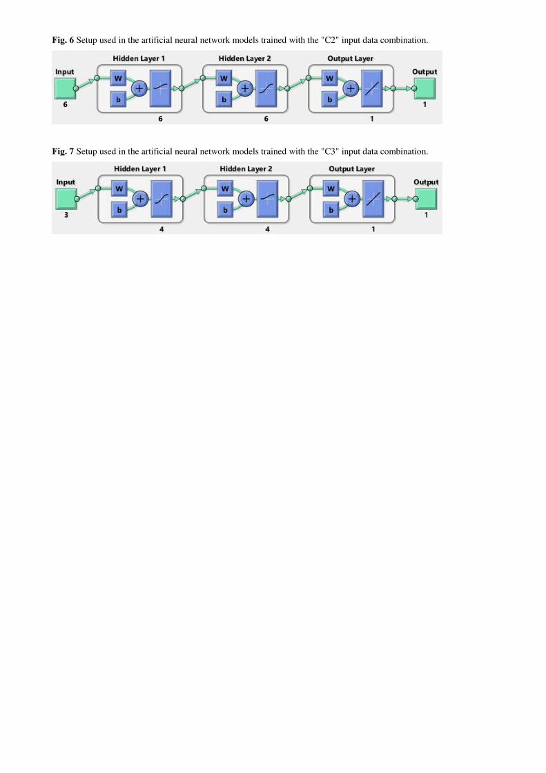
Fig. 6 Setup used in the artificial neural network models trained with the "C2" input data combination.
Fig. 7 Setup used in the artificial neural network models trained with the "C3" input data combination.