rainfall distribution in ethiopia - github...
TRANSCRIPT

Rainfall Distribution in Ethiopia
Mengying Li
Columbia University

1/30
Rainfall Distribution in Ethiopia
Abstract
By utilizing GIS and R, this study addresses some topics related to rainfall distribution in
Ethiopia. This paper is motivated by the payout mechanism of index insurance which aims at
reducing crop losses associated with weather uncertainty in low-income agricultural economies.
On the one hand, when it comes to the efficiency and inability of farmers, it is practically hard
for insurance companies to confirm crop losses door to door. On the other hand, if crop is mainly
affected by weather (e.g. if it suffers regularly from droughts or floods), we can base the payoff
design mainly on the related climate indicators, such as spatial correlation of rainfall, to ensure
that farmers affected by the same disaster get the same payoff. Rainfall is crucial for such an
agriculture-fed economy as Ethiopia where geography and climate are very variable. However,
different types of data, specifically, rain-gauge and satellite rainfall estimates, will yield different
results. My findings suggest that elevation has a positive impact on the rainfall in most areas of
Ethiopia. Rainfall has a strong clustering pattern. Different types of rainfall data will yield
different results when measuring the spatial distribution of rainfall. Space-time clusters could be
potentially used to validate the insurance payout complaints.
I. Introduction
Rainfall is a crucial determinant in agricultural economy as crop yield is vulnerable to
spatially and temporally uneven distribution of rainfall. Index insurance, aimed at protecting
farmers against climate uncertainty and encouraging banks to make loans for farmers, is
developed on the basis of statistics generated from historical records of rainfall distribution.
There are a lot of factors contributing to rainfall distribution patterns. Elevation is one of these

2/30
most important factors. In order to have a good knowledge of rainfall distribution, we need to
figure out its relationship with these geographical features.
The economy of Ethiopia is largely driven by rain-fed agriculture. However, Ethiopia is
located in the tropics and varies significantly in regional altitude (see Figure 1) , ranging from
210 m below sea level at the Denakil Depression in the northeast to over 4500 m above sea level
in the Simien Mountains in the north. As shown in Figure 2, rainfall levels fluctuate significantly
across time and space, which is typical of the progression of the Inter-Tropical Convergence
Zone (ITCZ). The greatest concentration of rainfall happens through July to August with 366
mm as the highest monthly level. The rainfall is very scarce in the southeastern lowlands, the
Ogaden Region, and the northeastern lowlands, the Danakil Desert. We can see that there is a lot
of overlap between the areas with high elevation and those with high levels of rainfall. And also
there seems to be a clear boundary between the rain-adequate areas and rain-scarce areas, which
implies the existence of clustering pattern.
Figure 1. Elevation in Ethiopia

3/30
Figure 2. Monthly Rainfall Distribution
This paper is organized as follows. Following this introduction, the next section describes
existing literature concerning rainfall study. The third section describes the methods used to
assess the statistical properties of rainfall distribution in Ethiopia. The fourth part concludes.
II. Literature Review

4/30
There are three rainfall seasons in Ethiopia, which are known as the Kiremt, Belga,and
Bega. The Kiremt season is the main rainy season and usually lasts from June to September,
covering all of Ethiopia except the southern and southeastern parts (Seleshi and Zanke, 2004).
The Belga season is the light rainy season and usually lasts from March to May and is the main
source of rainfall for the water-scarce southern and southeastern parts of Ethiopia (Seleshi and
Zanke, 2004). The Bega season is the dry season and usually lasts from October to February,
during which the entire country is dry, with the exception of occasional rainfall that is received
in the central sections (Seleshi and Zanke, 2004). Short cycle crops (e.g. wheat, teff, barley) that
are cultivated during the Belga and Kiremt seasons constitute 5 - 10% and 40 - 45% of national
crop production, respectively (Verdin et al., 2005). Long cycle crops, such as maize and sorghum,
are grown during the entire Belga and Kiremt seasons and are responsible for 50% of national
production (Verdin et al., 2005).
The timing, variability, and the quantity of seasonal and annual rainfall are important
factors in deciding the crop yield. If precipitation is unexpectedly low in the early growing
season, farmers may be able to resume production despite the loss of some of their crops (Hulme,
1990). However, if there is a rainfall break in the middle or latter growing season, all of the crops
may suffer from unrecoverable damage, causing direct economic loss for farmers (Hulme, 1990).
Spatial disparity of rainfall is largely caused by elevation. A high elevation usually leads
to low temperatures as the average regional temperature decreases by about 1o F for every 330 ft.
increase in altitude. As wet air rises, expands, and cools, it will reach its dew point (the
temperature at which condensation occurs) and form a cloud. If these condensed water particles
merge and become large enough they will fall as rain. According to Food and Agriculture
Organization (FAO) of the United Nations (1984), rainfall in Ethiopia is generally correlated
5/30
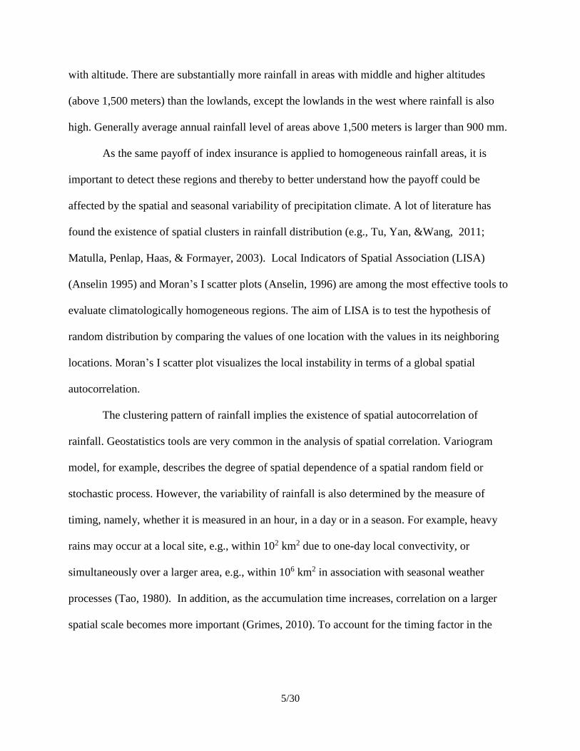
with altitude. There are substantially more rainfall in areas with middle and higher altitudes
(above 1,500 meters) than the lowlands, except the lowlands in the west where rainfall is also
high. Generally average annual rainfall level of areas above 1,500 meters is larger than 900 mm.
As the same payoff of index insurance is applied to homogeneous rainfall areas, it is
important to detect these regions and thereby to better understand how the payoff could be
affected by the spatial and seasonal variability of precipitation climate. A lot of literature has
found the existence of spatial clusters in rainfall distribution (e.g., Tu, Yan, &Wang, 2011;
Matulla, Penlap, Haas, & Formayer, 2003). Local Indicators of Spatial Association (LISA)
(Anselin 1995) and Moran’s I scatter plots (Anselin, 1996) are among the most effective tools to
evaluate climatologically homogeneous regions. The aim of LISA is to test the hypothesis of
random distribution by comparing the values of one location with the values in its neighboring
locations. Moran’s I scatter plot visualizes the local instability in terms of a global spatial
autocorrelation.
The clustering pattern of rainfall implies the existence of spatial autocorrelation of
rainfall. Geostatistics tools are very common in the analysis of spatial correlation. Variogram
model, for example, describes the degree of spatial dependence of a spatial random field or
stochastic process. However, the variability of rainfall is also determined by the measure of
timing, namely, whether it is measured in an hour, in a day or in a season. For example, heavy
rains may occur at a local site, e.g., within 102 km2 due to one-day local convectivity, or
simultaneously over a larger area, e.g., within 106 km2 in association with seasonal weather
processes (Tao, 1980). In addition, as the accumulation time increases, correlation on a larger
spatial scale becomes more important (Grimes, 2010). To account for the timing factor in the

6/30
variogram model, climatological variogram is therefore built up from the variograms in several
time intervals, each scaled by dividing by its variance (Grimes, 2010).
Different types of rainfall data might yield different results using the same variogram
model. Rain gauge data are collected from gauge stations, which give a direct picture of local
rainfall levels. However, these stations are unevenly distributed and located along main roads in
cities and towns, which limits the availability of rainfall data, especially in rural area where
rainfall information is more important to local residents. Gauge data also suffer from the problem
of gaps in the time series. Satellite proxies, particularly satellite rainfall estimate, have been used
as alternatives because of their availability even over remote parts of the world. However,
satellite rainfall estimates also suffer from a number of critical drawbacks, such as heterogeneous
time series, short time period of observation, and poor accuracy particularly at higher temporal
and spatial resolutions (Dinku, Hailemariam, Maidment, Tarnavsky and Connor, 2013). A good
understanding of the difference between these two data types in the estimation of spatial
distribution of rainfall will help us more precisely assess the regional rainfall homogeneity.
A lot of studies (e.g. Goovaerts, 2000) have shown that,when applied appropriately,
kriging is a more accurate interpolator of rainfall than other methods. A crucial element of the
kriging process is the calculation of a variogram which contains information on the variation
with distance of the correlation between two points.
III. Data and Methodology
The March rainfall in Ethiopia is going to be studied in this section as March is the
beginning month of the Belga season during which rains begin in the south and central parts of
the country.
3.1 Data

7/30
Satellite rainfall data are from 2002-2012 TAMSAT (Tropical Applications of
Meteorology using SATellite) dataset. It is a feature dataset. The data is collected using 10.8 μm
infra-red channel on the METEOSAT satellites and further calibrated by using a historical rain-
gauge dataset of > 17,000 stations in Africa. Different types of TAMSAT products, such as
decadal, monthly and seasonal data, are available. In order to compare the results generated from
different types of rainfall data, daily rainfall gauge data in March of 2002 – 2006 are also
introduced in this report. All the rainfall data are in millimeter.
Elevation data is from SRTM (Shuttle Radar Topography Mission) 3. It contains global
coverage from 56 degrees south latitude to 60 degrees north latitude in 1 by 1 degree blocks with
an approximate resolution of 90 by 90 meters. The data are in raster format and its unit is meter.
3.2 Rainfall and Elevation
In order to carry out regression analysis, the mean of elevation and rainfall level in each
polygon have to be calculated first. I used zonal statistics tool in ArcMap to calculate the mean
of elevation for each polygon in Ethiopia based on values from SRTM3 raster. As zonal statistics
tool can be only applied for raster data but the rainfall is a feature dataset, I first used the
conversion tool in ArcMap to convert it into a raster and then calculated the mean of March
rainfall in each polygon and merge these two datasets together into a feature dataset.
The statistical summary of dependent variable, rainfall, and independent variable,
elevation, is shown in Table 1. They are both regional average in each polygon.
Variable Mean Standard
Deviation
Minimum Maximum Number of
Observations
Rainfall (mm) 30.834 26.345 0 98.636 72
Elevation (m) 1600.95 577.557 388.881 2580.28 72
Table 1. Descriptive Statistics of Rainfall and Elevation

8/30
I start with a simple OLS model to quantify their relationship. The regression result is
shown in Table 2. Disappointingly, the coefficient of elevation is not statistically significant and
R-squared is only 0.021, which implies the misspecification of the model.
Moran's I (Moran 1950) statistics measures global spatial autocorrelation. Given a set of
locations and a corresponding variable, it evaluates whether the pattern in terms of that variable
is clustered, dispersed, or random. It is in the form of
2
0
( )( )
( )
ij i j
i j
i
i
w x x x xn
IS x x
,
where �̅� is the mean of the x variable, 𝑤𝑖𝑗 are the elements of the weight matrix, and 𝑆0 is the
sum of the elements of the weight matrix S0 = ∑ ∑ 𝑤𝑖𝑗𝑗𝑖 . In the presence of spatial correlation,
the absolute value of Moran’s I is close to 1.
In Table 3, we can see that the Moran’s I statistic is 0.8032 which is very close to 1 and
highly significant, suggesting the existence of spatial autocorrelation in the model. While
Moran’s I statistic has great power in detecting misspecifications in the model, it is less helpful
when it comes to the selection of a more appropriate model. The statistics generated from
Lagrange Multiplier test can be used to indicate a better model. We can see that the robust
version of Lagrange Multiplier statistics for the error model is more significant than the lag
model. So the spatial error model is used here and the result is shown in Table 4.
Variable Coefficient Std.Error t-Statistic Probability
Elevation 0.0066 0.0054 1.2300 0.22280
Constant 20.212* 9.1802 2.2017 0.03098
R-squared 0.021157

9/30
Note: *p < .05. **p < .01.
Table 2. OLS Regression
Table 3. Spatial Autocorrelation Test
Note: *p < .05. **p < .01.
Table 4. Spatial Error Model
In the spatial error model, a coefficient on the spatially correlated errors (LAMBDA) is
added as an additional indicator and it is highly significant. The independent variable, elevation,
also becomes statistically significant. The coefficient shows that one meter increase in elevation
increases rainfall level by 0.01032mm on average. As a result, the fitness of the model is
improved, as indicated in a higher value of R-squared.
Test MI/DF Value P-Value
Moran's I (error) 0.8032 10.9886 0.0000
Lagrange Multiplier
(lag) 1 101.6046 0.0000
Robust LM (lag) 1 1.036 0.3087
Lagrange Multiplier
(error) 1 104.3964 0.0000
Robust LM (error) 1 3.8278 0.0504
Lagrange Multiplier
(SARMA) 1 105.4324 0.0000
Variable Coefficient Std.Error z-value Probability
Elevation 0.01032** 0.002570 4.01482 0.0000595
Intercept 4.2011 41.8099 0.1005 0.9200
Lambda 0.9768** 0.01474 66.2746 0.0000
R-squared 0.9037

10/30
Geographically Weighted Regression (GWR) is further used to examine how spatially
consistent (stationary) the relationship between the rainfall level and elevation is across the study
area. The GWR result is shown in Table 5. We can see that the number of neighbors used for
local estimation is 17, which is dependent on the spatial density of rainfall and elevation. R-
squared is very high: 94.04% of rainfall variance is accounted for by the regression model.
Figure 3 visualizes the local relationship between elevation and rainfall level. By examining the
coefficient distribution, we can see where and how much variation is present. Though rainfall
increases with elevation in most parts of the country, there are also parts of the country where
rainfall decreases with elevation (blue shades in Figure 3). The negative relationship is mainly
distributed in the center of Ethiopia, where the altitude is also very high. This counterintuitive
result is mainly due to moisture depletion as most of the moisture fall out as rain before reaching
the top of the mountains (Dinku, Chidzambwa, Ceccato &Connor, 2008). However, the
distribution of the relationship between elevation and rainfall is a little bit different from the
finding of Dinku et al. (2008) (See Figure 4). In their paper, the most negative relationship is
shown to be in the northern and southern mountainous regions.
Neighbors 17
ResidualSquares 2978.17
EffectiveNumber 25.2912
Sigma 7.985
AICc 531.546
R2 0.9404
R2Adjusted 0.9094
Table 5 GWR Result

11/30
Figure 3. Distribution of Relationship between Rainfall and Elevation
Figure 4. Variation of Mean Annual Rainfall with Elevation
Source: Dinku, et al. (2008), p.4101.

12/30
3.3 Cluster of Rainfall
The diagnostic of spatial autocorrelation in the elevation analysis has shown that
neighboring rainfall exerts an effect on the rainfall itself through the error correlation. By
visualizing the LISA indicator, this clustering pattern of rainfall is shown in Figure 5. The
locations with significant local Moran statistics are shown in different colors based on the type of
spatial autocorrelation: red is for high-high and blue is for low-low. The high-high cluster is in
the southwest of Ethiopia and the north and east are low-low clusters.
The corresponding global Moran’s I statistic is 0.7862 and is very significant at 99.99%
level, which indicates a very strong spatial autocorrelation. However, it cannot discriminate
between a spatial clustering of high values and a spatial clustering of low values in the case of a
global positive spatial autocorrelation. So the scatter plot is used to specify different kinds of
autocorrelation (see Figure 6). The four different quadrants of the scatterplot correspond to the
four types of local spatial association between a region and its neighbors: HH, a region with a
high value surrounded by regions with high values (Quadrant I in top on the right); LH, a region
with low value surrounded by regions with high values (Quadrant II in top on the left); LL, a
region with a low value surrounded by regions with low values (Quadrant III in bottom on the
left); HL, a region with a high value surrounded by regions with low values (Quadrant IV in
bottom on the right). We can see that most of the points are in the Quadrant I and Quadrant III,
which is consistent with the positive Moran’s I statistics. Notably, there are more observations
with low-low clustering pattern than those with high-high clustering pattern.

13/30
Figure 5. LISA Cluster Map of March Rainfall in Ethiopia
Figure 6. Moran’s I Scatter Plot

14/30
3.4 Variogram and Climatological Variogram
The use of variogram is based on the concept that at a location, x, a dataset Z, can be
modeled as a slowly varying mean background, m, plus a random fluctuation, R
Z x=m x +R x
We now have a set of observations of Z, which in this case is rainfall level. For each pair
of points within this set, the distance between them can be recorded. Now for a given distance, h,
there are n subsets containing the pairs h apart (Goovaerts, 1997). The spatial dependence of the
subset can then be determined by calculating the variance of the difference between each pair.
After weighted by the number of pairs in each subset, the variogram is shown as below,
γ𝐡 =1
𝑛𝒉∑(𝑍𝑥𝑖
𝑛𝒉
𝑖
− 𝑍𝑥𝑖 + 𝒉)
For the statistical purpose, semivariogram is used in the paper, which is
𝛾∗𝐡 =1
2𝑛𝒉∑(𝑍𝑥𝑖
𝑛𝒉
𝑖
− 𝑍𝑥𝑖 + 𝒉)
The effect of rainfall is sensitive to the timing and specific event. The climatological
variogram is then calculated based on the assumption that the spatial correlation of rainfall
remains constant for a given region and time-period. The formula is shown as below, where k
refers to k time period and the previous semivariogram will be weighted by the variance of each
time period 𝜎𝑘2,
𝛾𝑐∗𝐡 =
1
𝐾∑
1
𝜎𝑘2
𝐾
𝑖=1
1
2𝑛𝒉∑(𝑍𝑥𝑖
𝑛𝒉
𝑖
− 𝑍𝑥𝑖 + 𝒉)

15/30
In this case, I am going to calculate the climatological variograms for both rain-gauge
and satellite data and compare the different results in terms of their relationship to the actual
rainfall intensity.
3.4.1 Gauge Data Result
The gauge stations in Oromiya area will be studied in this section. The location of gauge
stations is shown in Figure 7. In order to capture the detailed information as much as possible, a
2km distance lag is chosen for nonzero data. From Figure 8, we can see the number of pairs at
each binsize. For example, the first point is the number of pairs that in the first bin and the
second point is the number of pairs in the second bin. After 200km, the number of pairs in each
bin decreases as the distance increases. Based on Akaike Information Criterion (AIC) statistics,
the double spherical model is chosen over others (see Figure 9). The nugget is about 0.4. The
range is about 80 km, which implies when the distance exceeds 80 km, the spatial correlation
between different locations becomes weak. Notably, though the semivariance increases with the
distances, the change rate is not constant, with a turning point at about 15 km. There is more
noise at the end of the actual line as less data are available in each bin at a large distance.

16/30
Figure 7. Location of Gauge Station in Oromiya
Figure 8. Number of Location Pairs in each Bin (Binsize=2km)

17/30
Figure 9. Different Models of Daily Gauge Non-zero Data (Binsize=2 km)
3.4.2 Satellite Result
TAMSAT satellite estimates for the same locations as the gauges are analyzed in this
section. Using the same binsize as in the gauge case, we can see a large gap between these two
results. According to AIC, double spherical model best describes the variance in the data (see
Figure 11). Similarly, the relationship between the semivariogram and the distance is nonlinear
before it reaches the sill level, however, the turning point is almost 100km and the range is
almost 200 km. The result implies that remote technique seems to magnify the magnitude of
rainfall correlation.

18/30
Figure 10. Number of Location Pairs in each Bin (Binsize=2 km)
Figure 11. Different Models of Daily Satellite Data (Binsize=2)
We can visually compare the range calculated from variogram and the actual
rainfall distribution in Figure 12. We can see most of rainfall patches, the ones with the
same levels of rainfall are within 100 km.

19/30
Figure 12. The Scale of Actual Rainfall Patch
The reasons for the large gap between satellite and gauge estimates are complicated.
Most important one is the different mechanism of the measurement of gauges and satellites.
Gauges measure rainfall directly. However, the measurement always happens at a specific time
and only covers a small area. It also suffers from various problems, such as a poor spatial
sampling over unpopulated areas, temporal inhomogeneity in historical records, and uncertainty
associated with undercatchment1 due to the interaction with wind and evaporation (Chen, Xie,
1 Undercatchment by rain gages has been observed and studied since 1850. For instance, Symons (1866, 1880)
reported that a 6-meter elevated rain gage caught approximately 85% of the rainfall amount received on the ground,
and a rain gage installed on a church roof top of 45 meters above the ground experienced as much as a 50%
undercatch.

20/30
Janowiak, & Arkin, 2002). All these problems might lead to an underestimate of the actual
rainfall level and the variogram range within which rainfall are correlated. Satellite estimates
look at each pixel of the target area and are based on the movement of clouds over time, which
enable them to estimate rainfall levels in a wider area of and capture the dynamic change in the
structure of convective rainstorms. Satellites use the height of cloud top information as indicative
of rainfall; namely, they classify one area as rainy if the height of the cloud top is above a certain
threshold. However, it might give us the wrong information. For example, if one area is not
raining but the cloud top is high enough to reach the threshold, the satellite might mistake the
non-rainy area as rainy (see Figure 13). There are also two other possible explanations related to
the physical properties of the air masses as suggested by McCollum, Arnold and Mamoudou
(1999), which might lead to the overestimation in satellite data. One is that the possible existence
of aerosols in Africa leads to an abundance of cloud condensation nuclei, small drops, and
inefficient rain processes. The other is that “convective clouds forming under dry conditions
generally have cloud bases considerably higher than those of clouds forming in moist
environments. This leads to an increase in the evaporation rate of the falling rain, resulting in less
precipitation reaching the ground.” (McCollum, et al., 1999, p666). This overestimation might
imply a larger continuous surface of rainfall even the spatial autocorrelation is not that strong,
which will yield a large variogram range.

21/30
Figure 13. The Mechanism of TAMSAT Methodology
Note: Left: METEOSAT image of East Africa using the 10.8μm channel. The whiter the
image, the colder the cloud.
Right: Schematic TAMSAT methodology.
Source: H.L. Greatrex; “Satellite rainfall information in Africa”; Statistical Services
Centre, University of Reading, UK; Edition 1; 2012: P. 24
3.5 Kriging
Rainfall data are point data. It might be more in our interest to see the distribution
of rainfall over a surface, which will help us detect the possible pattern of rainfall, such
as cluster or trend.
Kriging, a geostatistical method to interpolate data in unsampled areas based on
the climatological variogram calculated from Section 3.4, will be discussed here.
Compared with traditional interpolation approaches, such as Inverse Distance
Weighted (IDW) interpolation, Kriging uses weights from semi-variogram rather than
applying an arbitrary or less precise weighting scheme. As Kriging associates some
probability with each prediction, hence it provides not just a surface, but some measure
of the accuracy of that surface, which is known as Kriging error. The kriging process
could be written in:
𝑍∗𝒉 − 𝑚𝒉 = ∑ 𝜆𝛼
𝑛
𝛼=1
|𝑍𝒉𝛼 − 𝑚𝒉𝛼|

22/30
Here, 𝒉 and 𝒉𝛼are vectors containing location information for estimation point
and the neighboring data points (indexed by α). Z(h) is treated as a random field, with a
trend m(u), and a residual component, R(h) = Z(h) - m(h). Kriging estimates the residual
at h as a weighted sum of the residuals at n surrounding data points. Kriging weights at
each surrounding point, λα, are derived from the semi-variogram (Bohling, 2005). This
equation can then be used to give a final estimate of Z(h) by minimizing the variance of
the estimator in a process described in detail in Goovaerts (1997). If a climatological
variogram has been used, the final kriging variance must also be re-scaled by
multiplying the result from each event by its variance.
3.5.1 Simple Kriging
Simple kriging assumes that the trend component is a constant over the entire
domain i.e. 𝑚𝒉 = 𝑚. Kriging with external drift, or universal kriging, caters for datasets
which have an underlying trend in the mean.
So far, all of these methods currently. It is computationally expensive to estimate
Z over many unsampled points and take an average if one wishes to know the value of Z
at a pixel. Instead, the process of block kriging can be used. This simply applies the
kriging methodology described above to find the average expected value in an area
around an un-sampled point, rather than the value at the point itself.
Here I used the rainfall data on three dates, specifically, March 15th, 2002, March
30th, 2004 and March 13th, 2005, as demos to show the simple kriging results. Two data
types, i.e. raw data and indicator rain gauge data (1 is for rainfall, 0 is for no rainfall)
were used on each day. The sample kriging results can be seen fromTable 6. The
semivariograms generated from indicator data can be shown in Figure 14. The
interpolation from indicator data gives the rainy probability of each location, ranging
from 0 to 1. We can see that the unsampled points close to the known location have a
similar value associated with them.
However, we can see that the ordinary kriging method suffers from several
problems. As the kriged value is mean-based, which implies that even an unsampled
point is far away from the input data, it will still be assigned a value as the mean. That’s
why some areas seem to be close to the no-rain locations and supposedly to be dry, or
distant from the sampling areas, still have non-zero values.

23/30
PointID Longitude Latitude Estimate1 Error1 Estimate2 Error2 Nearest
(km)
… … … … … … … …
A12911 39.144 7.019 11.35 5.35 2.07 0.67 28.3
A12912 39.181 7.019 11.35 5.35 2.12 0.67 24.1
A12913 39.219 7.019 11.34 5.34 2.17 0.66 20
A12914 39.256 7.019 11.31 5.34 2.22 0.65 15.9
A12915 39.294 7.019 11.26 5.32 2.27 0.63 11.7
A12916 39.331 7.019 11.16 5.26 2.32 0.6 7.6
A12917 39.369 7.019 11 5.11 2.38 0.58 3.5
A12918 39.406 7.019 10.81 4.86 2.42 0.55 0.7
A12919 39.444 7.019 10.92 5.03 2.44 0.56 4.8
A12920 39.481 7.019 11.1 5.23 2.46 0.58 9
A12921 39.519 7.019 11.22 5.31 2.47 0.6 13.1
A12922 39.556 7.019 11.29 5.33 2.48 0.61 17.2
A12923 39.594 7.019 11.32 5.34 2.49 0.62 21.1
A12924 39.631 7.019 11.34 5.35 2.51 0.62 17.5
A12925 39.669 7.019 11.34 5.35 2.52 0.61 14.1
A12926 39.706 7.019 11.35 5.35 2.54 0.59 11.3
A12927 39.744 7.019 11.35 5.35 2.57 0.56 9.4
A12928 39.781 7.019 11.35 5.35 2.59 0.55 9.2
A12929 39.819 7.019 11.35 5.35 2.6 0.55 10.7
A12930 39.856 7.019 11.35 5.35 2.62 0.55 13.4
… … … … … … … …
Table 6. Kriging Result Sample (March 15th, 2002)
Note: Estimate1 and error1 are from the kriging using raw data.
Estimate2 and error2 are from the kriging using indicator data.
Nearest means the nearest point from the kriged one.

24/30
Figure 14. Different Models of Daily Satellite Indicator Rainy Data (Binsize=2)
March 15th, 2002 March 30th, 2004 March 13th, 2005
Figure 15. Kriged Daily Rainfall for Oromiya (Raw Data)
25/30
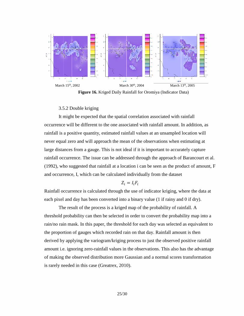
March 15th, 2002 March 30th, 2004 March 13th, 2005
Figure 16. Kriged Daily Rainfall for Oromiya (Indicator Data)
3.5.2 Double kriging
It might be expected that the spatial correlation associated with rainfall
occurrence will be different to the one associated with rainfall amount. In addition, as
rainfall is a positive quantity, estimated rainfall values at an unsampled location will
never equal zero and will approach the mean of the observations when estimating at
large distances from a gauge. This is not ideal if it is important to accurately capture
rainfall occurrence. The issue can be addressed through the approach of Barancourt et al.
(1992), who suggested that rainfall at a location i can be seen as the product of amount, F
and occurrence, I, which can be calculated individually from the dataset
𝑍𝑖 = 𝐼𝑖𝐹𝑖
Rainfall occurrence is calculated through the use of indicator kriging, where the data at
each pixel and day has been converted into a binary value (1 if rainy and 0 if dry).
The result of the process is a kriged map of the probability of rainfall. A
threshold probability can then be selected in order to convert the probability map into a
rain/no rain mask. In this paper, the threshold for each day was selected as equivalent to
the proportion of gauges which recorded rain on that day. Rainfall amount is then
derived by applying the variogram/kriging process to just the observed positive rainfall
amount i.e. ignoring zero-rainfall values in the observations. This also has the advantage
of making the observed distribution more Gaussian and a normal scores transformation
is rarely needed in this case (Greatrex, 2010).

26/30
The double kriged daily rainfall on these three days can be shown in Figure 17.
We can see that different from previous purely raw data and indicator kriging maps,
these double-kriged maps have the zero rainfall areas, which makes more sense.
March 15th, 2002 March 30th, 2004 March 13th, 2005
Figure 17. Double Kriged Daily Rainfall for Oromiya
IV. Further Development: Space-Time Cluster
Now, there are a lot of index insurance projects where stakeholders are asking to focus
on pixels over tens of thousands of sites (e.g Burkina), so it might make sense to start looking at
regional indices. Most complaints are from villages that neighboring villages got a different
payout from them but in fact they had the "same" year. Also, big events normally pay out over
large regions.
In order to specify the boundary of each “similar” area, I used SatScan for monthly
rainfall occurrence data from 1983-2013 in Tigray area in Ethiopia in an attempt to figure out the
possible space-time clusters. Figure 18-20 show the space-time clusters for June, August and
seasonal (June-September) rainfall occurrence. We can see that the “blue” and “red” clusters are
the most stable ones but the yellow and pink ones seem to be more sensitive to different time
dimensions. More interestingly, the north area of Tigray has a “non-clustering” cluster and it
turns out these areas are the ones with the strongest complaint about their payout they got from
the index insurance. It might be because that these areas don’t have a regular pattern in terms of
rainfall and their expectation from the index insurance might be biased.

27/30
Figure 18. Space-time Clusters for Rainfall Occurrence in Tigray (1983-2013)
V. Conclusion
This paper provides a framework of rainfall distribution in Ethiopia. A generally positive
relationship between rainfall and elevation has been found. However, the relationship does not
hold constant if we look at it locally; some parts might exhibit a negative impact of elevation on
rainfall. This inconsistency in rainfall-elevation relationship confirms the finding of Dinku
(2008). The estimates for the range of rainfall correlation using satellite data are more than twice
as large as them generated from gauge data. As index insurance is designed in such a way that
farmers in the areas where rainfall is spatially correlated will get the same payoff, a smaller
number of farmers are expected to get the payoff in face of the losses caused by rainfall if we
calculate the rainfall correlation on the basis of gauge data and a larger number getting the payoff
if the calculation is based on satellite data. Further work should be done in how to combine
these two estimates, i.e., gauge estimates and satellite estimates, to have a better estimate of
rainfall correlation and thereby to generate a more reasonable payoff for farmers.
This paper introduces different kriging methods using different types of data. We can see
that double kriging method yields a more reasonable result than ordinary kriging.
Besides the traditional clustering method, this paper further addresses the potential use of
space-time clusters to detect the areas which are suitable for collective purchase of the same type
of index insurance.
28/30
VI. References:
Bohling, G. (2005), Kriging, in Course notes for Data Analysis in Engineering and Natural
Science, edited, Kansas Geological Survey, Kansas.
Chen, M., Xie, P., Janowiak, J. E., & Arkin, P. A. (2002). Global land precipitation: A 50-yr
monthly analysis based on gauge observations. Journal of Hydrometeorology, 3(3), 249-
266.
Cheung, W. H., Senay, G. B., & Singh, A. (2008). Trends and spatial distribution of annual and
seasonal rainfall in Ethiopia. International journal of climatology, 28(13), 1723-1734.
Dinku, T., Chidzambwa, S., Ceccato, P., Connor, S. J., & Ropelewski, C. F. (2008). Validation
of high‐resolution satellite rainfall products over complex terrain. International Journal
of Remote Sensing, 29(14), 4097-4110.
Dinku, T., Hailemariam, K., Maidment, R., Tarnavsky, E., & Connor, S. (2013). Combined use
of satellite estimates and rain gauge observations to generate high‐quality historical
rainfall time series over Ethiopia. International Journal of Climatology.
Food and Agriculture Organization of the United Nations (1984). Agroclimatic Resource
Inventory for Land use Planning. Ethiopia. Technical Report 2. AG: DP/ETH/78/003,
Rome.
Greatrex, H., 2010. The application of seasonal rainfall forecasts and satellite rainfall
observations to crop yield forecasting for Africa. PhD thesis, University of Reading.

29/30
Grimes, D. I., & Pardo‐Igúzquiza, E. (2010). Geostatistical analysis of rainfall. Geographical
Analysis, 42(2), 136-160.
Goovaerts, P. (1997). Geostatistics for natural resources evaluation. Oxford university press.
Hulme, M. (1992). Rainfall changes in Africa: 1931–1960 to 1961–1990. International Journal
of Climatology, 12(7), 685-699.
Matulla, C., Penlap, E. K., Haas, P., & Formayer, H. (2003). Comparative analysis of spatial and
seasonal variability: Austrian precipitation during the 20th century. International Journal
of Climatology, 23(13), 1577-1588.
McCollum, Jeffrey R., Arnold, Gruber & Mamoudou, B. Ba (1999).Discrepancy between
Gauges and Satellite Estimates of Rainfall in Equatorial Africa. J. Appl. Meteor., 39,
666–679.
Moran, P. A. (1950). Notes on continuous stochastic phenomena. Biometrika, 37(1/2), 17-23.
Seleshi, Y., & Zanke, U. (2004). Recent changes in rainfall and rainy days in Ethiopia.
International Journal of Climatology, 24(8), 973-983.
Tao, S. (1980). Torrential Rain in China, Science Press, Beijing, 31–33.
Tu, K., Yan, Z. W., & Wang, Y. (2011). A spatial cluster analysis of heavy rains in China.
Atmos. Oceanic Sci. Lett, 4, 36-40.
University of Arizona School of Natural Resources and the Environment (2011). Elevation,
elevation, elevation. The Rimrock Report, 4(2) .

30/30
Verdin, J., Funk, C., Senay, G., & Choularton, R. (2005). Climate science and famine early
warning. Philosophical Transactions of the Royal Society B: Biological Sciences,
360(1463), 2155-2168