introduction to biocondcutor tools for second …jrojo/pasi/lectures/hector bio3.pdfintroduction to...
TRANSCRIPT
Introduction to Biocondcutor tools forsecond-generation sequencing analysis
Hector Corrada Bravobased on slides developed by
James Bullard Kasper Hansen and Margaret Taub
PASI Guanajuato MexicoMay 3-4 2010
1 1
Historical background previous sequencing-basedexpression measurements
I Serial analysis of gene expression (SAGE) has been around for awhile (Velculescu et al 1995) along with other methods such asmassively parallel signature sequencing (MPSS) and others
I SAGE data comes from selecting small ldquotagsrdquo one from each mRNAfragment then concatenating them and sequencing this long seriesof sequence fragments using Sanger sequencing Expression of agene is measured by counting how many times the tag from thatgene appears in the sequence
I In general the total number of tags sequenced per experiment isrelatively small (tens of thousands)
I Many statistical methods were developed in order to account forbiases in species detection facilitate combining reads across librariesand measure differential expression from the observed counts - moreon this later
2 1
Next Generation Sequencing NGS
I Illumina (Solexa) ldquoGenome Analyzer I and IIrdquo
I Roche (454) ldquoGenome Sequencerrdquo
I Applied Biosystems ldquoSOLiDrdquo
I Helicos ldquoHeliscoperdquo
There are many articleswebsites comparing the different technologieshowever the most prevalent platform appears to be Illumina at this pointPublications httpwwwilluminacompagesnrnilmnID=93
3 1
Applications of sequencing technology
High throughput sequencing has been used in many applications
I Resequencing
I De novo genome sequencing
I Tag-based expression analysis
I RNA-Seq expression analysis
I ChIP-Seq to detect transcription factor binding sites
I Methyl-Seq to detect DNA methylation sites
I Small RNA sequencing
I Ribosome profiling
I CLIP-Seq to detect protein-RNA interactions
4 1
Steps in analysis of sequencing data
The next lectures will walk through the steps needed to go from theoutput of the sequencing machine to abundance measurements forregions of interest We will focus on tools from Bioconductor althoughothers will be used as well We will cover
I Alignment
I Working with annotations (regions of interest)
I Aggregating counts to get a measure of abundance
5 1
A first quick look at the data
Data from two lanes of D melanogaster one wild-type and one where a splicing factor has been knocked down
(Data courtesy of Brenton Graveley)
6 1
Overview of Bioconductor NGS Packages
I IRanges provides low-level containers used by many of the otherBioconductor packages useful for working with annotation
I Biostrings provides complicated string processing methodsemphasis is placed on speed additionally provides a short readalignment tool matchPDict useful for mapping
I ShortRead provides functionality for processing NGS experimentsnamely reading in various aligned formats as well as lower-levelIllumina experiments useful for file IO mapping
I BSgenome provides tools for the ability to deal with genomes in Rtypically one uses a particular genome package such asBSgenomeScerevisiaeUCSCsacCer1 useful for mapping
I GenomeGraphs provides plotting functionality attached to liveannotation from Ensembl useful for visualization data qualityassessment results analysis
I biomaRt provides programmatic access to Ensembl and otherbiomart databases useful for working with annotation
I chipSeq provides tools for dealing with Chip-seq experiments
7 1
Overview of Bioconductor NGS Packages
I RTrackLayer provides access to various genome browsers useful forexamining results
8 1
Mapping
These slides will discuss mapping of sequence data as well as theBiostrings and ShortRead packages
I Alignment and tools (mostly external to R)
I Biostrings overview
I Alignment tools in Biostrings
I Mapping data and reading it into R
9 1
Alignment input FASTQ files
FASTQ files represent a common ldquoend-pointrdquo from the various sequencingplatforms (ie NCBI short read archivehttpwwwncbinlmnihgovTracessrasracgi) Qualities areencoded in ASCII and depending on the platform have slightly differentmeaningsranges and encoding More details can be found athttpenwikipediaorgwikiFASTQ_format
GA-EAS46_2_209DG61890752TTCTCTTAAGTCTTCTAGTTCTCTTCTTTCTCCACT+GA-EAS46_2_209DG61890752hhhhhhhhhhhhhhhhhhhhhhhhhhhhhhhhhhhhGA-EAS46_2_209DG61905558TCTGGCTTAACTTCTTCTTTTTTTTCTTCTTCTTCT+GA-EAS46_2_209DG61905558hhhfhhhhhhhhhhhhhhhhhhhhhhhhehhGhhJh
10 1
Alignment Tools
The number of short read aligners have exploded but a couple tools haveemerged as the de facto standards
I Eland Illuminarsquos aligner quality aware fast paired end capable
I MAQ Good SNP caller quality aware paired end capable
I Bowtie Super fast offers different alignment strategies paired endcapable
I BWA Fast indel support paired ends qualities
I NovoAlign MAQ like speed many features
A superior overview of the different aligners is available athttpwwwsangeracukUserslh3NGSalignshtml Additionallya comparison of two of the best aligners can be found here httpwwwmassgenomicsorg200907maq-bwa-and-bowtie-comparedhtml
11 1
Common Alignment Strategies
I Use qualities (default for Bowtie and MAQ)
I Perfect match no repeats (Strict Lenient)
I Mismatches no repeats
I Paired end data (PET) (harder for RNA-Seq)
The standard Illumina protocol yields unstranded reads
Most aligners are evaluated in terms of ldquohow many reads are mappedrdquo Isthis the right objective
Watch out for the output of the program there are many differentconventions (0-based what happens to read hitting the reverse strandetc)
12 1
SAMBAM Formats
SAM (BAM) is a new general format for storing mapped reads It isdeveloped as part of the 1000 Genomes project and is quickly becoming akind of standard Some alignment tools output this format directlyotherwise there are scripts in samtools for doing it for most popularaligners Details at httpsamtoolssourceforgenetindexshtml
13 1
A comment
There are no great comprehensive tools for analyzing deep-sequence dataIt will involve a fair amount of coding and gluing together various tools
We will introduce some tools from Bioconductor that can be useful
I use a lot of shell scripting
14 1
Biostrings overview
I A package for working with large (biological) strings
I Two main types of objects A really long single string (thinkchromosome) or a set of shorter strings (think reads or genes)BString vs BStringSet
I These classes are implemented efficiently minimizing copy andmemory loadingunloading
I The BSgenome contains some infrastructure for whole genomes
I Methods for dealing with biological data including basicmanipulation (complementation translation etc) string searching(exactinexact matching Smith-Waterman PWMs)
I Fairly complicated class structure
Irsquom sorry to say that at least for me this has becomehopelessly confusing and I imagine that many other usersfeel the same ndash Simon Anders on bioc-sig-sequencing
Computing on genomes is not trivial The approach to a givencomputation is important
15 1
Strings in Biostrings
I BString (general) DNAString RNAString AAString (Amino Acid)all examples of XString
I complement reverse reverseComplement translate for the classeswhere ldquoit makes senserdquo
I Convert to and from a standard R character string
I Constructor DNAString(ACGGGGG)
I Support for IUPAC alphabet
I Subsetting subseq using the SEW format (two out of the threestartendwidth) Efficient
I StringSets are collections of Strings like DNAStringSet
16 1
BSgenomes
As examples we will use whole genomes Use availablegenomes to getavailable genomes Long package names but always a shorter objectname
gt library(BSgenomeScerevisiaeUCSCsacCer1)
gt Scerevisiae
gt Scerevisiae[[1]]
gt Scerevisiae[[chr1]]
A BSgenome may also have masks We will ignore this for now
17 1
Biostrings more
I alphabetFrequency oligonucleotideFrequency and others
gt alphabetFrequency(Scerevisiae[[chr1]])
gt oligonucleotideFrequency(Scerevisiae[[chr1]]
+ width = 3)
I chartr for character translation (ldquomake all As into Csrdquo)
I Various IO functions (also ShortRead)
18 1
Views
A view is a set of substrings of an XString stored and manipulated veryefficiently Example to store exon sequences one can just store thegenomic location of the exons
gt Views(Scerevisiae[[chr1]] start = c(300
+ 400 500) width = 50)
A view is associated with a subject Internally they are essentiallyIRanges so they are very fast to compute with Views can in many casesbe treated exactly as other strings There are methods such as narrowtrim gaps restrict
19 1
Matching in Biostrings
There are various ways of matching or aligning strings to each other Weuse matching to denote searching for an exact match or possibly a matchwith a certain number of mismatches Alignment denotes a more generalstrategy eg Smith-Waterman
I matchPattern countPattern match 1 sequence to 1 sequence
I vmatchPattern vcountPattern match 1 sequence to manysequences
I pairwiseAlignment align many sequences to 1 sequence
I matchPDict countPDict match many sequences to 1 sequence(ldquodictrdquo indicates that the many sequences are preprocessed into adictionary)
I matchPWM trimLRpattern
The different functions are optimized for different situations They alsouse different algorithms which has a big impact EspeciallypairwiseAlignment is flexible and therefore has a complicated syntax
20 1
Example mapping probes to a genomeGet a list of Scerevisiae probes from the ldquoyeast2rdquo Affymetrix array
gt library(yeast2probe)
gt ids lt- scan(s_pombemsk skip = 2
+ what = list(probeset = character(0)
+ junk = character(0)))$probeset
gt probes lt- yeast2probe$sequence[yeast2probe$ProbeSetName in
+ ids]
gt probes lt- DNAStringSet(probes)
Mapping
gt require(BSgenomeScerevisiaeUCSCsacCer1)
gt dict0 lt- PDict(probes)
gt dict0r lt- PDict(reverseComplement(probes))
gt hits lt- matchPDict(dict0 Scerevisiae[[1]])
gt table(countIndex(hits))
gt table(countPDict(dict0 Scerevisiae[[1]]))
gt allhits lt- countPDict(dict0 Scerevisiae[[1]]) +
+ countPDict(dict0r Scerevisiae[[1]])
gt table(allhits)
21 1
ShortRead
ShortRead contains tools for
I Work with Illumina output
I Generate QA report on Illumina files
I Read a variety of short read data formats
22 1
Data
We will use data from (Lee Hansen Bullard Dudoit and Sherlock(2008) PLoS Genetics)
We are considering a wild-type and a mutant strain of yeast The twostrains were sequenced using an Illumina Genome Analyzer
We are using a subset of the data 100K reads from a single lane for onestrain
23 1
Reading the unaligned data
gt require(ShortRead)
gt fq lt- readFastq( mut_1_ffastqgz$)
gt fq
There are various simple accessor functions for this object especiallysread and quality
24 1
A brief look at the unaligned data
Using alphabetByCycle and as( rdquomatrixrdquo) (which creates a big read timescycle matrix) we can do
gt alp lt- alphabetByCycle(sread(fq))
gt matplot(t(proptable(alp[DNA_BASES
+ ] margin = 2)) type = l)
gt qaMatraw lt- as(quality(fq) matrix)
gt plot(colMeans(qaMatraw))
25 1
Alphabet By Cycle plot
26 1
Mean Quality per Cycle
27 1
Reading in the aligned data
We read data aligned with bowtie into R as a AlignedRead object
gt aligned lt- readAligned( pattern = bowtiegz$
+ type = Bowtie)
gt aligned
28 1
Getting abundance data for regions of interest
I We want to get our data in a form where we can measure abundancefor regions of interest (eg transcript abundance in genes)
I We have already mapped our reads to our reference genome so weknow what position they originated from
I Next we need to work with the genome annotation and produceregion-level summaries
I We start by importing the annotation into R so that we can workwith it there
29 1
Working with annotation
We need to obtain annotation for our organism Using Bioconductor thiscan be done with the biomaRt package This package allows us todirectly download information from Ensembl using the biomaRt interface
gt require(biomaRt)
gt mart lt- useMart(ensembl scerevisiae_gene_ensembl)
gt yeastAnno lt- getBM(c(ensembl_gene_id
+ chromosome_name start_position
+ end_position strand gene_biotype)
+ mart = mart)
gt head(yeastAnno 2)
30 1
Data Representation
Currently we have the data stored where each line in our data filerepresents a unique read Often we want to count the number of readsthat overlap or start at a given position One easy way to do this is touse the pileup function from ShortRead
gt keep lt- chromosome(aligned) ==
+ Scchr01
gt ll lt- seqlengths(Scerevisiae)
gt names(ll) lt- levels(chromosome(aligned))
gt cov lt- coverage(aligned[keep]
+ width = ll)
I What type of object is returned
31 1
Plotting coverage
gt cov lt- asnumeric(cov)
gt keep lt- cov gt 0
gt Indices lt- (1length(cov))[keep]
gt plot(Indices cov[keep] col = blue
+ type = h ylim = c(0 100)
+ xlab = Chromosome Position
+ ylab = Coverage)
32 1
Plotting Coverage
33 1
Associating Annotation to Reads
At an abstract level we want to apply a function that associates thealigned read data to the relevant regions of annotation and then countsthe number of reads that fall into each gene This will be our measure ofgene expression
First we need to determine in which range each read lands At the endof the day we want a data structure that looks more or less like this
mut_1 mut_2 wt_1 wt_2YHR055C 0 0 0 0YPR161C 38 39 35 34YOL138C 31 33 40 26YDR395W 55 52 47 47YGR129W 29 26 5 5YPR165W 189 180 151 180
34 1
IRanges
I An IRange is a set of integer ranges 1minus 4 7minus 10 45minus 89 Theranges can be overlapping or not and are stored as (start endwidth)
I Every range can be specified using 2 out of (start end width)
I This has proved to be a very general class of objects Examplesgene (annotation in general) DNA reads
I A NormalIRanges is a minimal representation (in some sense) notempty non-overlapping non-empty gap ordered They areimportant for computational reasons
I Many methods for IRanges are very fast Some computations can besped up dramatically by converting the underlying objects intoIRanges do the computation and then convert back
35 1
Some examples of IRanges functions
In our case the integer ranges we are interested in are the base positionsbetween the start and end position of the yeast genes But the package ismuch more general and can be used for other kinds of analysis as wellAs a simple example
gt ir1 lt- IRanges(start = 15 end = 610)
gt ir2 lt- IRanges(start = 412 width = 5)
gt union(ir1 ir2)
gt intersect(ir1 ir2)
gt findOverlaps(ir1 ir2)
gt astable(findOverlaps(ir1 ir2))
36 1
Some more details on overlap
The function findOverlaps can be confusing at first The syntax isfindOverlaps(querysubject) and you can think of the result as abinary matrix with length(query) rows and length(subject)columns The return value you see is simply a ldquosparserdquo representation ofthis matrix giving only the coordinates of the non-zero elements
Additionally overlap can be called on two RangesList objects of thesame length The resulting object is a list of objects of classRangesMatching
37 1
Using IRanges to represent our annotation
First we need to match the chromosome names as Ensembl uses romannumerals and the Bowtie index used names
gt cNames lt- levels(chromosome(aligned[[1]]))
gt names(cNames) lt- c(ascharacter(asroman(116))
+ NA)
gt yeastAnno$chr lt- cNames[yeastAnno$chr]
gt yeastAnno lt- yeastAnno[isna(yeastAnno$chr)
+ ]
Now we construct a set of IRanges which represent our genes Since theIRanges class only includes a start a stop and a width we need oneIRanges object for each chromosome In the last step we construct aRangesList object which will be useful for our next steps
38 1
Using IRanges to represent our annotation
gt annoByChr lt- split(yeastAnno yeastAnno$chr)
gt iL lt- lapply(annoByChr function(d)
+ IRanges(start = d$start_position
+ end = d$end_position)
+ )
gt iL lt- docall(RangesList iL)
gt iL
39 1
Representing our reads as IRanges
Next we convert our aligned reads into IRanges as well Again we needa separate IRanges object for each chromosome and they are arrangedinto a RangesList
gt alnAsRanges lt- as(aligned RangesList)
gt alnAsRanges
40 1
Counting reads that fall in our genes
Finally we use the astable and countOverlaps in order to compute thecounts within each gene (removing reads from the mitochondrialgenome) Unfortunately this operation doesnrsquot yet do the right thingwith names so we have to add the names back at the end not elegant
gt alnAsRanges lt- alnAsRanges[-length(alnAsRanges)]
gt oCounts lt- lapply(countOverlaps(alnAsRanges
+ iL) astable)
gt geneNames lt- split(yeastAnno$ensembl_gene_id
+ yeastAnno$chr)[-c(1 7)]
gt o lt- order(asinteger(asroman(names(geneNames))))
gt geneNames lt- geneNames[o]
gt oCounts lt- mapply(FUN = function(cnts
+ nms)
+ names(cnts) lt- nms
+ cnts
+ oCounts geneNames)
gt lapply(oCounts head)
41 1

Overview of Bioconductor NGS Packages
I RTrackLayer provides access to various genome browsers useful forexamining results
8 1
Mapping
These slides will discuss mapping of sequence data as well as theBiostrings and ShortRead packages
I Alignment and tools (mostly external to R)
I Biostrings overview
I Alignment tools in Biostrings
I Mapping data and reading it into R
9 1
Alignment input FASTQ files
FASTQ files represent a common ldquoend-pointrdquo from the various sequencingplatforms (ie NCBI short read archivehttpwwwncbinlmnihgovTracessrasracgi) Qualities areencoded in ASCII and depending on the platform have slightly differentmeaningsranges and encoding More details can be found athttpenwikipediaorgwikiFASTQ_format
GA-EAS46_2_209DG61890752TTCTCTTAAGTCTTCTAGTTCTCTTCTTTCTCCACT+GA-EAS46_2_209DG61890752hhhhhhhhhhhhhhhhhhhhhhhhhhhhhhhhhhhhGA-EAS46_2_209DG61905558TCTGGCTTAACTTCTTCTTTTTTTTCTTCTTCTTCT+GA-EAS46_2_209DG61905558hhhfhhhhhhhhhhhhhhhhhhhhhhhhehhGhhJh
10 1
Alignment Tools
The number of short read aligners have exploded but a couple tools haveemerged as the de facto standards
I Eland Illuminarsquos aligner quality aware fast paired end capable
I MAQ Good SNP caller quality aware paired end capable
I Bowtie Super fast offers different alignment strategies paired endcapable
I BWA Fast indel support paired ends qualities
I NovoAlign MAQ like speed many features
A superior overview of the different aligners is available athttpwwwsangeracukUserslh3NGSalignshtml Additionallya comparison of two of the best aligners can be found here httpwwwmassgenomicsorg200907maq-bwa-and-bowtie-comparedhtml
11 1
Common Alignment Strategies
I Use qualities (default for Bowtie and MAQ)
I Perfect match no repeats (Strict Lenient)
I Mismatches no repeats
I Paired end data (PET) (harder for RNA-Seq)
The standard Illumina protocol yields unstranded reads
Most aligners are evaluated in terms of ldquohow many reads are mappedrdquo Isthis the right objective
Watch out for the output of the program there are many differentconventions (0-based what happens to read hitting the reverse strandetc)
12 1
SAMBAM Formats
SAM (BAM) is a new general format for storing mapped reads It isdeveloped as part of the 1000 Genomes project and is quickly becoming akind of standard Some alignment tools output this format directlyotherwise there are scripts in samtools for doing it for most popularaligners Details at httpsamtoolssourceforgenetindexshtml
13 1
A comment
There are no great comprehensive tools for analyzing deep-sequence dataIt will involve a fair amount of coding and gluing together various tools
We will introduce some tools from Bioconductor that can be useful
I use a lot of shell scripting
14 1
Biostrings overview
I A package for working with large (biological) strings
I Two main types of objects A really long single string (thinkchromosome) or a set of shorter strings (think reads or genes)BString vs BStringSet
I These classes are implemented efficiently minimizing copy andmemory loadingunloading
I The BSgenome contains some infrastructure for whole genomes
I Methods for dealing with biological data including basicmanipulation (complementation translation etc) string searching(exactinexact matching Smith-Waterman PWMs)
I Fairly complicated class structure
Irsquom sorry to say that at least for me this has becomehopelessly confusing and I imagine that many other usersfeel the same ndash Simon Anders on bioc-sig-sequencing
Computing on genomes is not trivial The approach to a givencomputation is important
15 1
Strings in Biostrings
I BString (general) DNAString RNAString AAString (Amino Acid)all examples of XString
I complement reverse reverseComplement translate for the classeswhere ldquoit makes senserdquo
I Convert to and from a standard R character string
I Constructor DNAString(ACGGGGG)
I Support for IUPAC alphabet
I Subsetting subseq using the SEW format (two out of the threestartendwidth) Efficient
I StringSets are collections of Strings like DNAStringSet
16 1
BSgenomes
As examples we will use whole genomes Use availablegenomes to getavailable genomes Long package names but always a shorter objectname
gt library(BSgenomeScerevisiaeUCSCsacCer1)
gt Scerevisiae
gt Scerevisiae[[1]]
gt Scerevisiae[[chr1]]
A BSgenome may also have masks We will ignore this for now
17 1
Biostrings more
I alphabetFrequency oligonucleotideFrequency and others
gt alphabetFrequency(Scerevisiae[[chr1]])
gt oligonucleotideFrequency(Scerevisiae[[chr1]]
+ width = 3)
I chartr for character translation (ldquomake all As into Csrdquo)
I Various IO functions (also ShortRead)
18 1
Views
A view is a set of substrings of an XString stored and manipulated veryefficiently Example to store exon sequences one can just store thegenomic location of the exons
gt Views(Scerevisiae[[chr1]] start = c(300
+ 400 500) width = 50)
A view is associated with a subject Internally they are essentiallyIRanges so they are very fast to compute with Views can in many casesbe treated exactly as other strings There are methods such as narrowtrim gaps restrict
19 1
Matching in Biostrings
There are various ways of matching or aligning strings to each other Weuse matching to denote searching for an exact match or possibly a matchwith a certain number of mismatches Alignment denotes a more generalstrategy eg Smith-Waterman
I matchPattern countPattern match 1 sequence to 1 sequence
I vmatchPattern vcountPattern match 1 sequence to manysequences
I pairwiseAlignment align many sequences to 1 sequence
I matchPDict countPDict match many sequences to 1 sequence(ldquodictrdquo indicates that the many sequences are preprocessed into adictionary)
I matchPWM trimLRpattern
The different functions are optimized for different situations They alsouse different algorithms which has a big impact EspeciallypairwiseAlignment is flexible and therefore has a complicated syntax
20 1
Example mapping probes to a genomeGet a list of Scerevisiae probes from the ldquoyeast2rdquo Affymetrix array
gt library(yeast2probe)
gt ids lt- scan(s_pombemsk skip = 2
+ what = list(probeset = character(0)
+ junk = character(0)))$probeset
gt probes lt- yeast2probe$sequence[yeast2probe$ProbeSetName in
+ ids]
gt probes lt- DNAStringSet(probes)
Mapping
gt require(BSgenomeScerevisiaeUCSCsacCer1)
gt dict0 lt- PDict(probes)
gt dict0r lt- PDict(reverseComplement(probes))
gt hits lt- matchPDict(dict0 Scerevisiae[[1]])
gt table(countIndex(hits))
gt table(countPDict(dict0 Scerevisiae[[1]]))
gt allhits lt- countPDict(dict0 Scerevisiae[[1]]) +
+ countPDict(dict0r Scerevisiae[[1]])
gt table(allhits)
21 1
ShortRead
ShortRead contains tools for
I Work with Illumina output
I Generate QA report on Illumina files
I Read a variety of short read data formats
22 1
Data
We will use data from (Lee Hansen Bullard Dudoit and Sherlock(2008) PLoS Genetics)
We are considering a wild-type and a mutant strain of yeast The twostrains were sequenced using an Illumina Genome Analyzer
We are using a subset of the data 100K reads from a single lane for onestrain
23 1
Reading the unaligned data
gt require(ShortRead)
gt fq lt- readFastq( mut_1_ffastqgz$)
gt fq
There are various simple accessor functions for this object especiallysread and quality
24 1
A brief look at the unaligned data
Using alphabetByCycle and as( rdquomatrixrdquo) (which creates a big read timescycle matrix) we can do
gt alp lt- alphabetByCycle(sread(fq))
gt matplot(t(proptable(alp[DNA_BASES
+ ] margin = 2)) type = l)
gt qaMatraw lt- as(quality(fq) matrix)
gt plot(colMeans(qaMatraw))
25 1
Alphabet By Cycle plot
26 1
Mean Quality per Cycle
27 1
Reading in the aligned data
We read data aligned with bowtie into R as a AlignedRead object
gt aligned lt- readAligned( pattern = bowtiegz$
+ type = Bowtie)
gt aligned
28 1
Getting abundance data for regions of interest
I We want to get our data in a form where we can measure abundancefor regions of interest (eg transcript abundance in genes)
I We have already mapped our reads to our reference genome so weknow what position they originated from
I Next we need to work with the genome annotation and produceregion-level summaries
I We start by importing the annotation into R so that we can workwith it there
29 1
Working with annotation
We need to obtain annotation for our organism Using Bioconductor thiscan be done with the biomaRt package This package allows us todirectly download information from Ensembl using the biomaRt interface
gt require(biomaRt)
gt mart lt- useMart(ensembl scerevisiae_gene_ensembl)
gt yeastAnno lt- getBM(c(ensembl_gene_id
+ chromosome_name start_position
+ end_position strand gene_biotype)
+ mart = mart)
gt head(yeastAnno 2)
30 1
Data Representation
Currently we have the data stored where each line in our data filerepresents a unique read Often we want to count the number of readsthat overlap or start at a given position One easy way to do this is touse the pileup function from ShortRead
gt keep lt- chromosome(aligned) ==
+ Scchr01
gt ll lt- seqlengths(Scerevisiae)
gt names(ll) lt- levels(chromosome(aligned))
gt cov lt- coverage(aligned[keep]
+ width = ll)
I What type of object is returned
31 1
Plotting coverage
gt cov lt- asnumeric(cov)
gt keep lt- cov gt 0
gt Indices lt- (1length(cov))[keep]
gt plot(Indices cov[keep] col = blue
+ type = h ylim = c(0 100)
+ xlab = Chromosome Position
+ ylab = Coverage)
32 1
Plotting Coverage
33 1
Associating Annotation to Reads
At an abstract level we want to apply a function that associates thealigned read data to the relevant regions of annotation and then countsthe number of reads that fall into each gene This will be our measure ofgene expression
First we need to determine in which range each read lands At the endof the day we want a data structure that looks more or less like this
mut_1 mut_2 wt_1 wt_2YHR055C 0 0 0 0YPR161C 38 39 35 34YOL138C 31 33 40 26YDR395W 55 52 47 47YGR129W 29 26 5 5YPR165W 189 180 151 180
34 1
IRanges
I An IRange is a set of integer ranges 1minus 4 7minus 10 45minus 89 Theranges can be overlapping or not and are stored as (start endwidth)
I Every range can be specified using 2 out of (start end width)
I This has proved to be a very general class of objects Examplesgene (annotation in general) DNA reads
I A NormalIRanges is a minimal representation (in some sense) notempty non-overlapping non-empty gap ordered They areimportant for computational reasons
I Many methods for IRanges are very fast Some computations can besped up dramatically by converting the underlying objects intoIRanges do the computation and then convert back
35 1
Some examples of IRanges functions
In our case the integer ranges we are interested in are the base positionsbetween the start and end position of the yeast genes But the package ismuch more general and can be used for other kinds of analysis as wellAs a simple example
gt ir1 lt- IRanges(start = 15 end = 610)
gt ir2 lt- IRanges(start = 412 width = 5)
gt union(ir1 ir2)
gt intersect(ir1 ir2)
gt findOverlaps(ir1 ir2)
gt astable(findOverlaps(ir1 ir2))
36 1
Some more details on overlap
The function findOverlaps can be confusing at first The syntax isfindOverlaps(querysubject) and you can think of the result as abinary matrix with length(query) rows and length(subject)columns The return value you see is simply a ldquosparserdquo representation ofthis matrix giving only the coordinates of the non-zero elements
Additionally overlap can be called on two RangesList objects of thesame length The resulting object is a list of objects of classRangesMatching
37 1
Using IRanges to represent our annotation
First we need to match the chromosome names as Ensembl uses romannumerals and the Bowtie index used names
gt cNames lt- levels(chromosome(aligned[[1]]))
gt names(cNames) lt- c(ascharacter(asroman(116))
+ NA)
gt yeastAnno$chr lt- cNames[yeastAnno$chr]
gt yeastAnno lt- yeastAnno[isna(yeastAnno$chr)
+ ]
Now we construct a set of IRanges which represent our genes Since theIRanges class only includes a start a stop and a width we need oneIRanges object for each chromosome In the last step we construct aRangesList object which will be useful for our next steps
38 1
Using IRanges to represent our annotation
gt annoByChr lt- split(yeastAnno yeastAnno$chr)
gt iL lt- lapply(annoByChr function(d)
+ IRanges(start = d$start_position
+ end = d$end_position)
+ )
gt iL lt- docall(RangesList iL)
gt iL
39 1
Representing our reads as IRanges
Next we convert our aligned reads into IRanges as well Again we needa separate IRanges object for each chromosome and they are arrangedinto a RangesList
gt alnAsRanges lt- as(aligned RangesList)
gt alnAsRanges
40 1
Counting reads that fall in our genes
Finally we use the astable and countOverlaps in order to compute thecounts within each gene (removing reads from the mitochondrialgenome) Unfortunately this operation doesnrsquot yet do the right thingwith names so we have to add the names back at the end not elegant
gt alnAsRanges lt- alnAsRanges[-length(alnAsRanges)]
gt oCounts lt- lapply(countOverlaps(alnAsRanges
+ iL) astable)
gt geneNames lt- split(yeastAnno$ensembl_gene_id
+ yeastAnno$chr)[-c(1 7)]
gt o lt- order(asinteger(asroman(names(geneNames))))
gt geneNames lt- geneNames[o]
gt oCounts lt- mapply(FUN = function(cnts
+ nms)
+ names(cnts) lt- nms
+ cnts
+ oCounts geneNames)
gt lapply(oCounts head)
41 1

Mapping
These slides will discuss mapping of sequence data as well as theBiostrings and ShortRead packages
I Alignment and tools (mostly external to R)
I Biostrings overview
I Alignment tools in Biostrings
I Mapping data and reading it into R
9 1
Alignment input FASTQ files
FASTQ files represent a common ldquoend-pointrdquo from the various sequencingplatforms (ie NCBI short read archivehttpwwwncbinlmnihgovTracessrasracgi) Qualities areencoded in ASCII and depending on the platform have slightly differentmeaningsranges and encoding More details can be found athttpenwikipediaorgwikiFASTQ_format
GA-EAS46_2_209DG61890752TTCTCTTAAGTCTTCTAGTTCTCTTCTTTCTCCACT+GA-EAS46_2_209DG61890752hhhhhhhhhhhhhhhhhhhhhhhhhhhhhhhhhhhhGA-EAS46_2_209DG61905558TCTGGCTTAACTTCTTCTTTTTTTTCTTCTTCTTCT+GA-EAS46_2_209DG61905558hhhfhhhhhhhhhhhhhhhhhhhhhhhhehhGhhJh
10 1
Alignment Tools
The number of short read aligners have exploded but a couple tools haveemerged as the de facto standards
I Eland Illuminarsquos aligner quality aware fast paired end capable
I MAQ Good SNP caller quality aware paired end capable
I Bowtie Super fast offers different alignment strategies paired endcapable
I BWA Fast indel support paired ends qualities
I NovoAlign MAQ like speed many features
A superior overview of the different aligners is available athttpwwwsangeracukUserslh3NGSalignshtml Additionallya comparison of two of the best aligners can be found here httpwwwmassgenomicsorg200907maq-bwa-and-bowtie-comparedhtml
11 1
Common Alignment Strategies
I Use qualities (default for Bowtie and MAQ)
I Perfect match no repeats (Strict Lenient)
I Mismatches no repeats
I Paired end data (PET) (harder for RNA-Seq)
The standard Illumina protocol yields unstranded reads
Most aligners are evaluated in terms of ldquohow many reads are mappedrdquo Isthis the right objective
Watch out for the output of the program there are many differentconventions (0-based what happens to read hitting the reverse strandetc)
12 1
SAMBAM Formats
SAM (BAM) is a new general format for storing mapped reads It isdeveloped as part of the 1000 Genomes project and is quickly becoming akind of standard Some alignment tools output this format directlyotherwise there are scripts in samtools for doing it for most popularaligners Details at httpsamtoolssourceforgenetindexshtml
13 1
A comment
There are no great comprehensive tools for analyzing deep-sequence dataIt will involve a fair amount of coding and gluing together various tools
We will introduce some tools from Bioconductor that can be useful
I use a lot of shell scripting
14 1
Biostrings overview
I A package for working with large (biological) strings
I Two main types of objects A really long single string (thinkchromosome) or a set of shorter strings (think reads or genes)BString vs BStringSet
I These classes are implemented efficiently minimizing copy andmemory loadingunloading
I The BSgenome contains some infrastructure for whole genomes
I Methods for dealing with biological data including basicmanipulation (complementation translation etc) string searching(exactinexact matching Smith-Waterman PWMs)
I Fairly complicated class structure
Irsquom sorry to say that at least for me this has becomehopelessly confusing and I imagine that many other usersfeel the same ndash Simon Anders on bioc-sig-sequencing
Computing on genomes is not trivial The approach to a givencomputation is important
15 1
Strings in Biostrings
I BString (general) DNAString RNAString AAString (Amino Acid)all examples of XString
I complement reverse reverseComplement translate for the classeswhere ldquoit makes senserdquo
I Convert to and from a standard R character string
I Constructor DNAString(ACGGGGG)
I Support for IUPAC alphabet
I Subsetting subseq using the SEW format (two out of the threestartendwidth) Efficient
I StringSets are collections of Strings like DNAStringSet
16 1
BSgenomes
As examples we will use whole genomes Use availablegenomes to getavailable genomes Long package names but always a shorter objectname
gt library(BSgenomeScerevisiaeUCSCsacCer1)
gt Scerevisiae
gt Scerevisiae[[1]]
gt Scerevisiae[[chr1]]
A BSgenome may also have masks We will ignore this for now
17 1
Biostrings more
I alphabetFrequency oligonucleotideFrequency and others
gt alphabetFrequency(Scerevisiae[[chr1]])
gt oligonucleotideFrequency(Scerevisiae[[chr1]]
+ width = 3)
I chartr for character translation (ldquomake all As into Csrdquo)
I Various IO functions (also ShortRead)
18 1
Views
A view is a set of substrings of an XString stored and manipulated veryefficiently Example to store exon sequences one can just store thegenomic location of the exons
gt Views(Scerevisiae[[chr1]] start = c(300
+ 400 500) width = 50)
A view is associated with a subject Internally they are essentiallyIRanges so they are very fast to compute with Views can in many casesbe treated exactly as other strings There are methods such as narrowtrim gaps restrict
19 1
Matching in Biostrings
There are various ways of matching or aligning strings to each other Weuse matching to denote searching for an exact match or possibly a matchwith a certain number of mismatches Alignment denotes a more generalstrategy eg Smith-Waterman
I matchPattern countPattern match 1 sequence to 1 sequence
I vmatchPattern vcountPattern match 1 sequence to manysequences
I pairwiseAlignment align many sequences to 1 sequence
I matchPDict countPDict match many sequences to 1 sequence(ldquodictrdquo indicates that the many sequences are preprocessed into adictionary)
I matchPWM trimLRpattern
The different functions are optimized for different situations They alsouse different algorithms which has a big impact EspeciallypairwiseAlignment is flexible and therefore has a complicated syntax
20 1
Example mapping probes to a genomeGet a list of Scerevisiae probes from the ldquoyeast2rdquo Affymetrix array
gt library(yeast2probe)
gt ids lt- scan(s_pombemsk skip = 2
+ what = list(probeset = character(0)
+ junk = character(0)))$probeset
gt probes lt- yeast2probe$sequence[yeast2probe$ProbeSetName in
+ ids]
gt probes lt- DNAStringSet(probes)
Mapping
gt require(BSgenomeScerevisiaeUCSCsacCer1)
gt dict0 lt- PDict(probes)
gt dict0r lt- PDict(reverseComplement(probes))
gt hits lt- matchPDict(dict0 Scerevisiae[[1]])
gt table(countIndex(hits))
gt table(countPDict(dict0 Scerevisiae[[1]]))
gt allhits lt- countPDict(dict0 Scerevisiae[[1]]) +
+ countPDict(dict0r Scerevisiae[[1]])
gt table(allhits)
21 1
ShortRead
ShortRead contains tools for
I Work with Illumina output
I Generate QA report on Illumina files
I Read a variety of short read data formats
22 1
Data
We will use data from (Lee Hansen Bullard Dudoit and Sherlock(2008) PLoS Genetics)
We are considering a wild-type and a mutant strain of yeast The twostrains were sequenced using an Illumina Genome Analyzer
We are using a subset of the data 100K reads from a single lane for onestrain
23 1
Reading the unaligned data
gt require(ShortRead)
gt fq lt- readFastq( mut_1_ffastqgz$)
gt fq
There are various simple accessor functions for this object especiallysread and quality
24 1
A brief look at the unaligned data
Using alphabetByCycle and as( rdquomatrixrdquo) (which creates a big read timescycle matrix) we can do
gt alp lt- alphabetByCycle(sread(fq))
gt matplot(t(proptable(alp[DNA_BASES
+ ] margin = 2)) type = l)
gt qaMatraw lt- as(quality(fq) matrix)
gt plot(colMeans(qaMatraw))
25 1
Alphabet By Cycle plot
26 1
Mean Quality per Cycle
27 1
Reading in the aligned data
We read data aligned with bowtie into R as a AlignedRead object
gt aligned lt- readAligned( pattern = bowtiegz$
+ type = Bowtie)
gt aligned
28 1
Getting abundance data for regions of interest
I We want to get our data in a form where we can measure abundancefor regions of interest (eg transcript abundance in genes)
I We have already mapped our reads to our reference genome so weknow what position they originated from
I Next we need to work with the genome annotation and produceregion-level summaries
I We start by importing the annotation into R so that we can workwith it there
29 1
Working with annotation
We need to obtain annotation for our organism Using Bioconductor thiscan be done with the biomaRt package This package allows us todirectly download information from Ensembl using the biomaRt interface
gt require(biomaRt)
gt mart lt- useMart(ensembl scerevisiae_gene_ensembl)
gt yeastAnno lt- getBM(c(ensembl_gene_id
+ chromosome_name start_position
+ end_position strand gene_biotype)
+ mart = mart)
gt head(yeastAnno 2)
30 1
Data Representation
Currently we have the data stored where each line in our data filerepresents a unique read Often we want to count the number of readsthat overlap or start at a given position One easy way to do this is touse the pileup function from ShortRead
gt keep lt- chromosome(aligned) ==
+ Scchr01
gt ll lt- seqlengths(Scerevisiae)
gt names(ll) lt- levels(chromosome(aligned))
gt cov lt- coverage(aligned[keep]
+ width = ll)
I What type of object is returned
31 1
Plotting coverage
gt cov lt- asnumeric(cov)
gt keep lt- cov gt 0
gt Indices lt- (1length(cov))[keep]
gt plot(Indices cov[keep] col = blue
+ type = h ylim = c(0 100)
+ xlab = Chromosome Position
+ ylab = Coverage)
32 1
Plotting Coverage
33 1
Associating Annotation to Reads
At an abstract level we want to apply a function that associates thealigned read data to the relevant regions of annotation and then countsthe number of reads that fall into each gene This will be our measure ofgene expression
First we need to determine in which range each read lands At the endof the day we want a data structure that looks more or less like this
mut_1 mut_2 wt_1 wt_2YHR055C 0 0 0 0YPR161C 38 39 35 34YOL138C 31 33 40 26YDR395W 55 52 47 47YGR129W 29 26 5 5YPR165W 189 180 151 180
34 1
IRanges
I An IRange is a set of integer ranges 1minus 4 7minus 10 45minus 89 Theranges can be overlapping or not and are stored as (start endwidth)
I Every range can be specified using 2 out of (start end width)
I This has proved to be a very general class of objects Examplesgene (annotation in general) DNA reads
I A NormalIRanges is a minimal representation (in some sense) notempty non-overlapping non-empty gap ordered They areimportant for computational reasons
I Many methods for IRanges are very fast Some computations can besped up dramatically by converting the underlying objects intoIRanges do the computation and then convert back
35 1
Some examples of IRanges functions
In our case the integer ranges we are interested in are the base positionsbetween the start and end position of the yeast genes But the package ismuch more general and can be used for other kinds of analysis as wellAs a simple example
gt ir1 lt- IRanges(start = 15 end = 610)
gt ir2 lt- IRanges(start = 412 width = 5)
gt union(ir1 ir2)
gt intersect(ir1 ir2)
gt findOverlaps(ir1 ir2)
gt astable(findOverlaps(ir1 ir2))
36 1
Some more details on overlap
The function findOverlaps can be confusing at first The syntax isfindOverlaps(querysubject) and you can think of the result as abinary matrix with length(query) rows and length(subject)columns The return value you see is simply a ldquosparserdquo representation ofthis matrix giving only the coordinates of the non-zero elements
Additionally overlap can be called on two RangesList objects of thesame length The resulting object is a list of objects of classRangesMatching
37 1
Using IRanges to represent our annotation
First we need to match the chromosome names as Ensembl uses romannumerals and the Bowtie index used names
gt cNames lt- levels(chromosome(aligned[[1]]))
gt names(cNames) lt- c(ascharacter(asroman(116))
+ NA)
gt yeastAnno$chr lt- cNames[yeastAnno$chr]
gt yeastAnno lt- yeastAnno[isna(yeastAnno$chr)
+ ]
Now we construct a set of IRanges which represent our genes Since theIRanges class only includes a start a stop and a width we need oneIRanges object for each chromosome In the last step we construct aRangesList object which will be useful for our next steps
38 1
Using IRanges to represent our annotation
gt annoByChr lt- split(yeastAnno yeastAnno$chr)
gt iL lt- lapply(annoByChr function(d)
+ IRanges(start = d$start_position
+ end = d$end_position)
+ )
gt iL lt- docall(RangesList iL)
gt iL
39 1
Representing our reads as IRanges
Next we convert our aligned reads into IRanges as well Again we needa separate IRanges object for each chromosome and they are arrangedinto a RangesList
gt alnAsRanges lt- as(aligned RangesList)
gt alnAsRanges
40 1
Counting reads that fall in our genes
Finally we use the astable and countOverlaps in order to compute thecounts within each gene (removing reads from the mitochondrialgenome) Unfortunately this operation doesnrsquot yet do the right thingwith names so we have to add the names back at the end not elegant
gt alnAsRanges lt- alnAsRanges[-length(alnAsRanges)]
gt oCounts lt- lapply(countOverlaps(alnAsRanges
+ iL) astable)
gt geneNames lt- split(yeastAnno$ensembl_gene_id
+ yeastAnno$chr)[-c(1 7)]
gt o lt- order(asinteger(asroman(names(geneNames))))
gt geneNames lt- geneNames[o]
gt oCounts lt- mapply(FUN = function(cnts
+ nms)
+ names(cnts) lt- nms
+ cnts
+ oCounts geneNames)
gt lapply(oCounts head)
41 1
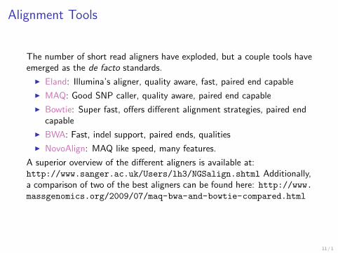
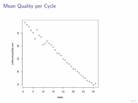
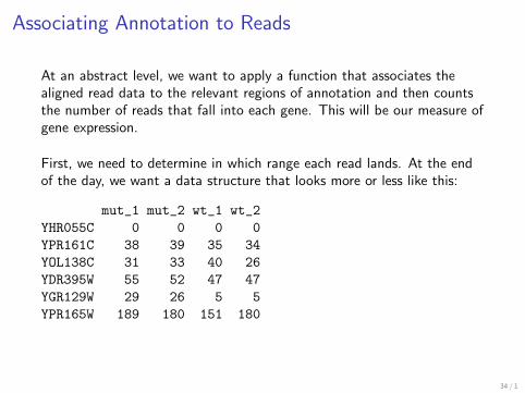

Using IRanges to represent our annotation
gt annoByChr lt- split(yeastAnno yeastAnno$chr)
gt iL lt- lapply(annoByChr function(d)
+ IRanges(start = d$start_position
+ end = d$end_position)
+ )
gt iL lt- docall(RangesList iL)
gt iL
39 1
Representing our reads as IRanges
Next we convert our aligned reads into IRanges as well Again we needa separate IRanges object for each chromosome and they are arrangedinto a RangesList
gt alnAsRanges lt- as(aligned RangesList)
gt alnAsRanges
40 1
Counting reads that fall in our genes
Finally we use the astable and countOverlaps in order to compute thecounts within each gene (removing reads from the mitochondrialgenome) Unfortunately this operation doesnrsquot yet do the right thingwith names so we have to add the names back at the end not elegant
gt alnAsRanges lt- alnAsRanges[-length(alnAsRanges)]
gt oCounts lt- lapply(countOverlaps(alnAsRanges
+ iL) astable)
gt geneNames lt- split(yeastAnno$ensembl_gene_id
+ yeastAnno$chr)[-c(1 7)]
gt o lt- order(asinteger(asroman(names(geneNames))))
gt geneNames lt- geneNames[o]
gt oCounts lt- mapply(FUN = function(cnts
+ nms)
+ names(cnts) lt- nms
+ cnts
+ oCounts geneNames)
gt lapply(oCounts head)
41 1