introduction to di erential geometry -...

Introduction to Differential Geometry

Ivan Izmestiev

University of Fribourg, Spring 2016

Contents

1 Curvature of curves 1

1 Curves, length, and area . . . . . . . . . . . . . . . . . . . . . . . . . . . . 1

1.1 What is a curve? . . . . . . . . . . . . . . . . . . . . . . . . . . . . 1

1.2 Length of a smooth curve . . . . . . . . . . . . . . . . . . . . . . . 3

1.3 Area enclosed by a smooth planar curve . . . . . . . . . . . . . . . 5

2 Curvature . . . . . . . . . . . . . . . . . . . . . . . . . . . . . . . . . . . . 6

2.1 Regular curves . . . . . . . . . . . . . . . . . . . . . . . . . . . . . 6

2.2 Arc-length parametrization . . . . . . . . . . . . . . . . . . . . . . 6

2.3 Curvature and osculating circles . . . . . . . . . . . . . . . . . . . 8

2 Plane curves 10

1 Evolutes and wave fronts . . . . . . . . . . . . . . . . . . . . . . . . . . . . 10

1.1 Signed curvature . . . . . . . . . . . . . . . . . . . . . . . . . . . . 10

1.2 Evolutes and involutes . . . . . . . . . . . . . . . . . . . . . . . . . 11

1.3 Parallel curves and wave fronts . . . . . . . . . . . . . . . . . . . . 13

1.4 Distance functions . . . . . . . . . . . . . . . . . . . . . . . . . . . 14

2 Rotation index and convex curves . . . . . . . . . . . . . . . . . . . . . . . 16

2.1 The total signed curvature . . . . . . . . . . . . . . . . . . . . . . . 16

2.2 Rotation of simple closed curves . . . . . . . . . . . . . . . . . . . 17

2.3 Convex curves . . . . . . . . . . . . . . . . . . . . . . . . . . . . . 17

2.4 Convex curves in polar coordinates . . . . . . . . . . . . . . . . . . 18

3 Global geometry of plane curves . . . . . . . . . . . . . . . . . . . . . . . 18

3.1 Support function . . . . . . . . . . . . . . . . . . . . . . . . . . . . 18

3.2 The average width . . . . . . . . . . . . . . . . . . . . . . . . . . . 19

3.3 Isoperimetric inequality . . . . . . . . . . . . . . . . . . . . . . . . 20

3.4 Steiner formulas . . . . . . . . . . . . . . . . . . . . . . . . . . . . 21

3.5 Gauss map . . . . . . . . . . . . . . . . . . . . . . . . . . . . . . . 22

3.6 Minkowski formulas . . . . . . . . . . . . . . . . . . . . . . . . . . 23

3.7 Four-vertex theorem . . . . . . . . . . . . . . . . . . . . . . . . . . 23

3.8 Steiner point . . . . . . . . . . . . . . . . . . . . . . . . . . . . . . 24

i

ii CONTENTS

3 Space curves 261 Torsion . . . . . . . . . . . . . . . . . . . . . . . . . . . . . . . . . . . . . 26

1.1 Frenet formulas . . . . . . . . . . . . . . . . . . . . . . . . . . . . . 261.2 Osculating plane and osculating sphere . . . . . . . . . . . . . . . 271.3 Existence and uniqueness theorems . . . . . . . . . . . . . . . . . . 28

2 Global geometry of space curves . . . . . . . . . . . . . . . . . . . . . . . 282.1 Curves on the sphere . . . . . . . . . . . . . . . . . . . . . . . . . . 282.2 Fenchel theorem . . . . . . . . . . . . . . . . . . . . . . . . . . . . 302.3 Weyl tube formula . . . . . . . . . . . . . . . . . . . . . . . . . . . 31

4 Surfaces: the first fundamental form 331 Definitions and examples . . . . . . . . . . . . . . . . . . . . . . . . . . . . 33

1.1 What is a surface? . . . . . . . . . . . . . . . . . . . . . . . . . . . 331.2 Examples . . . . . . . . . . . . . . . . . . . . . . . . . . . . . . . . 341.3 Smooth surfaces . . . . . . . . . . . . . . . . . . . . . . . . . . . . 35

2 Measuring lengths and areas . . . . . . . . . . . . . . . . . . . . . . . . . . 352.1 Lengths of curves on surfaces . . . . . . . . . . . . . . . . . . . . . 352.2 Isometries . . . . . . . . . . . . . . . . . . . . . . . . . . . . . . . . 362.3 Conformal maps . . . . . . . . . . . . . . . . . . . . . . . . . . . . 362.4 Surface area . . . . . . . . . . . . . . . . . . . . . . . . . . . . . . . 36

5 Curvature of surfaces 371 The second fundamental form . . . . . . . . . . . . . . . . . . . . . . . . . 37

1.1 Deviation from the tangent plane . . . . . . . . . . . . . . . . . . . 371.2 The curvature of curves on a surface . . . . . . . . . . . . . . . . . 38

2 Principal curvatures . . . . . . . . . . . . . . . . . . . . . . . . . . . . . . 392.1 Definition . . . . . . . . . . . . . . . . . . . . . . . . . . . . . . . . 392.2 Curvature of surfaces of revolution . . . . . . . . . . . . . . . . . . 392.3 Curvature lines and triply orthogonal systems . . . . . . . . . . . . 392.4 The shape operator and the Weingarten matrix . . . . . . . . . . . 39

3 The Gaussian curvature and the mean curvature . . . . . . . . . . . . . . 403.1 Definitions and formulas . . . . . . . . . . . . . . . . . . . . . . . . 403.2 The third fundamental form . . . . . . . . . . . . . . . . . . . . . . 403.3 The Gauss map and the Gauss-Bonnet theorem for convex surfaces 403.4 Covariant differentiation . . . . . . . . . . . . . . . . . . . . . . . . 403.5 Hessian and Laplacian . . . . . . . . . . . . . . . . . . . . . . . . . 41

4 Parallel surfaces . . . . . . . . . . . . . . . . . . . . . . . . . . . . . . . . . 424.1 Curvature of parallel surfaces . . . . . . . . . . . . . . . . . . . . . 424.2 Delaunay surfaces . . . . . . . . . . . . . . . . . . . . . . . . . . . 434.3 Weyl tube formula . . . . . . . . . . . . . . . . . . . . . . . . . . . 434.4 Steiner formula . . . . . . . . . . . . . . . . . . . . . . . . . . . . . 44

5 Differential geometry of convex bodies . . . . . . . . . . . . . . . . . . . . 445.1 The support function . . . . . . . . . . . . . . . . . . . . . . . . . 445.2 Volume in terms of the support function . . . . . . . . . . . . . . . 45

CONTENTS iii

5.3 Minkowski formulas . . . . . . . . . . . . . . . . . . . . . . . . . . 465.4 Spherical harmonics . . . . . . . . . . . . . . . . . . . . . . . . . . 475.5 Spherical Laplacian and the Poincare-Wirtinger inequality . . . . . 475.6 Support function and curvature . . . . . . . . . . . . . . . . . . . . 475.7 On the isoperimetric inequality . . . . . . . . . . . . . . . . . . . . 47

6 Minimal surfaces . . . . . . . . . . . . . . . . . . . . . . . . . . . . . . . . 476.1 Divergence, rate of the volume change, and the mean curvature . . 476.2 Definition and examples of minimal surfaces . . . . . . . . . . . . . 496.3 Conformal harmonic parametrizations . . . . . . . . . . . . . . . . 496.4 Laplacian and conformal maps . . . . . . . . . . . . . . . . . . . . 506.5 Adjoint minimal surface . . . . . . . . . . . . . . . . . . . . . . . . 516.6 Associate family of minimal surfaces . . . . . . . . . . . . . . . . . 526.7 Minimal surfaces and isotropic holomorphic curves in C3 . . . . . . 526.8 Enneper-Weierstrass representation . . . . . . . . . . . . . . . . . . 53

6 Geodesics 551 Definition and variational properties . . . . . . . . . . . . . . . . . . . . . 55

1.1 Curves of vanishing geodesic curvature . . . . . . . . . . . . . . . . 551.2 Geodesic equations and their consequences . . . . . . . . . . . . . 561.3 The energy and the length functionals . . . . . . . . . . . . . . . . 58

2 Geodesic coordinates . . . . . . . . . . . . . . . . . . . . . . . . . . . . . . 602.1 Geodesic polar coordinates . . . . . . . . . . . . . . . . . . . . . . 602.2 Local length minimization . . . . . . . . . . . . . . . . . . . . . . . 602.3 Geodesic normal coordinates . . . . . . . . . . . . . . . . . . . . . 61

3 Geodesics on special surfaces . . . . . . . . . . . . . . . . . . . . . . . . . 623.1 Surfaces of revolution . . . . . . . . . . . . . . . . . . . . . . . . . 623.2 Distance functions . . . . . . . . . . . . . . . . . . . . . . . . . . . 633.3 Geodesics on Liouville surfaces . . . . . . . . . . . . . . . . . . . . 653.4 Some theorems on ellipses and ellipsoids . . . . . . . . . . . . . . . 66

7 Fundamental equations of the surface theory 671 Theorema Egregium . . . . . . . . . . . . . . . . . . . . . . . . . . . . . . 67

1.1 Extrinsic and intrinsic objects . . . . . . . . . . . . . . . . . . . . . 671.2 The intrinsic nature of the covariant derivative . . . . . . . . . . . 671.3 Linear and differential operators . . . . . . . . . . . . . . . . . . . 681.4 The curvature tensor . . . . . . . . . . . . . . . . . . . . . . . . . . 701.5 Proof of the Theorema Egregium . . . . . . . . . . . . . . . . . . . 70

2 Applications of Theorema Egregium . . . . . . . . . . . . . . . . . . . . . 71

iv CONTENTS

Chapter 1

Curvature of curves

1 Curves, length, and area

1.1 What is a curve?

We will study curves in the plane or in the space. There are different ways to describea curve.

• Graph of a function:

y = f(x) (plane curve)

{y = f(x)z = g(x)

(space curve)

Problem: not every curve is a graph of a function (think of a circle or of a spiral).

• Level set of a function:

F (x, y) = c (plane curve)

In R3 the level set of a function is (usually) a surface. A curve can be representedas an intersection of two surfaces:{

F1(x, y) = c1

F2(x, y) = c2

This is good enough, but not convenient for computations (we will see this later).

• Parametrized curve: trajectory of a point. This is the most convenient represen-tation, and we will use it most of the time.

Definition 1.1. A parametrized curve is a map from an interval to Rn:

γ : I → Rn,

where I ⊂ R is (a, b) or (−∞, b) or (−∞,+∞) or [a, b] etc.

1

2 CHAPTER 1. CURVATURE OF CURVES

Example 1.2. • A graph of a function can easily be parametrized:

y = f(x)⇔{

x = ty = f(t)

That is, we put γ(t) = (t, f(t)).

• The circle x2 + y2 = 1 can be parametrized as

x = cos t, y = sin t

As the range of t we can take [0, 2π) or (−∞,+∞). The latter traces the circleinfinitely many times.

Exercise 1.3. Find a parametrization of the curve x2 − y2 = 1 (this set consists of twocomponents; parametrize one of them).

Note that the parametrization of a curve is not unique: different maps can have thesame images. For example, the upper semicircle can be parametrized as

γ(t) = (t,√

1− t2), t ∈ [−1, 1]

The parabola y = x2 can be parametrized as (t, t2) or, for example, as (t3, t6).Having decided for parametrized curves, let us think how good the map γ should be

so that it image could be called a “curve”. Of course, we want γ to be continuous (thepoint is moving, not jumping). But there are continuous maps that look rather strange...

• Space-filling curves, e. g. Peano curve and Hilbert curve. They map an intervalonto a square (surjectively, but not injectively).

• The Koch snowflake. The boundary of the Koch snowflake is an injective image ofa circle. However it has an infinite length.

Exercise 1.4. Compute the perimeter of the n-th iteration of the Koch snowflake.Compute the area of the Koch snowflake.

Remark 1.5. The boundary of the Koch snowflake has Hausdorff dimension log 4log 3 > 1,

so this is not quite a curve. Objects of non-integer dimension are called fractals. Somebeautiful pictures of fractals can be found in the book [MSW02].

Since we are doing differential geometry, we will require the map γ to be differen-tiable.

Definition 1.6. A parametrized curve γ : I → Rn is called smooth if it is a C∞-map.

By this we mean that each component of γ can be differentiated any number of times:

if γ(t) = (γ1(t), . . . , γn(t)), then all of the derivatives dγidt , d2γi

dt2, d3γidt3

, . . . do exist.The derivative of γ

γ =dγ

dt=

(dγ1

dt, . . . ,

dγndt

)is called the velocity vector of γ.

https://en.wikipedia.org/wiki/Peano_curve

https://en.wikipedia.org/wiki/Hilbert_curve

https://en.wikipedia.org/wiki/Koch_snowflake

Curves, length, and area 3

1.2 Length of a smooth curve

The velocity vector shows the direction and the speed of the motion. The distancetraveled is the speed multiplied by the time. If the speed is variable, then the distanceis the integral of the speed as a function of the time. Thus the common sense suggestsus the following

Definition 1.7. The integral

L(γ) =

b∫a

‖γ‖ dt =

b∫a

√(dγ1

dt

)2

+ · · ·+(dγndt

)2

dt

is called the length of a smooth curve γ : [a, b]→ Rn.

There is a theorem behind this definition, because a standard way to define the lengthof a curve is as the supremum of lengths of inscribed polygons (think of how the lengthof a circle is defined):

L(γ) := supT

n∑i=1

‖γ(ti)− γ(ti−1)‖, (1.1)

where T denotes a subdivision a = t0 < t1 < · · · < tn = b.

Theorem 1.8. For every smooth curve γ : [a, b]→ Rn the supremum (1.1) exists and isequal to the integral in Definition 1.7:

L(γ) = L(γ).

We need a lemma.

Lemma 1.9. For every smooth curve γ : [a, b] → Rn its length is bigger or equal thanthe distance between the endpoints:∫ b

a‖γ‖ dt ≥ ‖γ(b)− γ(a)‖

Proof. Use the Cauchy-Schwarz inequality:

‖γ(b)− γ(a)‖‖γ‖ ≥ 〈γ(b)− γ(a), γ〉

Integration yields

‖γ(b)−γ(a)‖∫ b

a‖γ‖ dt ≥

⟨γ(b)− γ(a),

∫ b

aγ dt

⟩= 〈γ(b)−γ(a), γ(b)−γ(a) = ‖γ(b)−γ(a)‖2

and the lemma follows.


Proof of Theorem 1.8. For any subdivision T denote by LT the length of the correspond-ing polygon and by γtiti−1

the arc of γ between ti−1 and ti. By Lemma 1.9 we have

L(γ) =n∑i=1

L(γtiti−1) ≥

n∑i=1

‖γ(ti)− γ(ti−1)‖ = LT

As a consequence, L(γ) = supT LT exists, and L(γ) ≤ L(γ).

Denote S(t) = L(γta) and compute the derivative of S(t). It is easily seen that thegeneralized length is additive: S(t+ ε)− S(t) = L(γt+εt ) for ε ≥ 0. Hence we have∥∥∥∥γ(t+ ε)− γ(t)

ε

∥∥∥∥ ≤ S(t+ ε)− S(t)

ε≤ 1

ε

∫ t+ε

t‖γ‖ dt

(Check that this is also valid for ε < 0.) As ε tends to 0, both the left hand side andthe right hand side tend to γ(t), and we conclude that the function S(t) is differentiablewith dS

dt = ‖γ‖. Since S(a) = 0, it follows that

L(γ) = S(b) =

∫ b

a‖γ‖ dt = L(γ).

Remark 1.10. Curves for which the supremum of lengths of inscribed polygons existare called rectifiable. The Peano curve, the Hilbert curve, and the Koch curve are notrectifiable. It can be shown that every Lipschitz curve is rectifiable.

Definition 1.11. Roll a circle along a line. The curve traced by a point on the circle iscalled a cycloid.

Let the line be the x-axis, the circle have radius 1, at t = 0 the circle be tangent to thex-axis at the origin, and the point which we follow lie at the origin at this moment. If thecircle rolls with a constant speed, then the corresponding cycloid has the parametrization

γ(t) = (t− sin t, 1− cos t)

Exercise 1.12. Check the above equation. Compute the velocity vectors at t = 0 andnear t = 0. Sketch the cycloid.

Exercise 1.13. Compute the length of the cycloid arc t ∈ [0, 2π]. When you ride abicycle, what is the ratio between the distance traveled by you and the distance traveledby a point on a tire?

Curves, length, and area 5

1.3 Area enclosed by a smooth planar curve

In this section we speak only about plane curves.A curve γ : [a, b]→ R2 is called closed, if γ(a) = γ(b). A closed curve is called simple,

if it is not self-intersecting: γ(t) = γ(t′)⇒ t = t′ or {t, t′} = {a, b}.Denote by A(int(γ)) the area of the region bounded by a simple closed plane curve

γ. Let us derive a formula for A(int(γ)) heuristically. Consider a subdivision a < t1 <t2 < · · · < tn = b. The area of the polygon PT with the vertices γ(t1), . . . , γ(tn) equals

n∑i=1

area(Oγ(ti)γ(ti+1)) =1

2

n∑i=1

Oγ(ti)×Oγ(ti+1) =1

2

n∑i=1

(x(ti)y(ti+1)− x(ti+1)y(ti)

Here v × w denotes the planar cross-product, which is half the (signed) area of thetriangle spanned by the vectors v and w. A different way to write the area of PT is

1

2

n∑i=1

γ(ti)× (γ(ti+1)− γ(ti))

Intuitively, as the subdivision becomes finer, the above sum should tend to the integralof γ × γ. Also the areas of inscribed polygons should tend to the area of the regioninside γ. We don’t prove either of these statements. Instead, we use a different methodto prove the formula that we have just conjectured.

Theorem 1.14. Let γ : [a, b] → R2 be a simple closed curve. If γ is oriented counter-clockwise, then the area of the region bounded by γ equals

area(int(γ)) =1

2

∫ b

a(γ × γ) dt =

1

2

∫ b

a(xy − xy) dt (1.2)

If γ is oriented clockwise, then the above integral equals minus the area bounded by γ.

Proof. Recall the Green theorem:∫int(γ)

(∂g

∂x− ∂f

∂y

)dxdy =

∫γf dx+ g dy

Put f(x, y) = −y and g(x, y) = x. Then the left hand side equals twice the area, andthe right hand side equals∫

γ(−y) dx+ x dy =

∫ b

a(−yx+ xy) dt

Exercise 1.15. Show that if the curve γ is not closed, then formula (1.2) gives the(signed) area of the region bounded by γ and the segments Oγ(a) and Oγ(b).

What is the geometric meaning of formula (1.2) in the case when γ has self-intersections?

Exercise 1.16. Compute the area under an arc of the cycloid.


2 Curvature

2.1 Regular curves

Even a smooth curve doesn’t always “look smooth”. We see it on the example of acycloid that has sharp points at t = 2kπ (a cusp). Another typical example is thesemicubical parabola y = x2/3 which has a smooth parametrization γ(t) = (t3, t2) butexhibits a cusp at the point (0, 0).

Exercise 2.1. Find a smooth parametrization of the curve y = |x|.

The problem with these points is that γ vanishes.

Definition 2.2. A point γ(t) on a parametrized curve γ is called a regular point ifγ(t) 6= 0; otherwise γ(t) is called a singular point. A curve is called regular if all of itspoints are regular.

There is a whole branch of mathematics that studies singularities of smooth maps; foran introduction see [Bro75]. We will focus on regular curves (or regular arcs of curves).

Exercise 2.3. The curveγ(t) = (cos3 t, sin3 t)

is called astroid. Find singular and regular points of the astroid. Sketch the curve.

Exercise 2.4. Compute the length of the astroid and the area enclosed by it.

A parametrized curve possesses an oriented tangent at each of its regular points. Theequation of the tangent at γ(t0) is

`(t) = γ(t0) + tγ(t0)

(Note that at a cusp point there is also a tangent, but it has no orientation compatiblewith the time parameter on the curve.)

2.2 Arc-length parametrization

Definition 2.5. Let γ : I → Rn be a smooth curve. A reparametrization of γ is a curve

γ : J → Rn, where γ = γ ◦ ϕ

and ϕ : J → I is a diffeomorphism (that is, a differentiable bijective map with differen-tiable inverse).

Clearly, if γ is a reparametrization of γ, then γ is a reparametrization of γ.

Example 2.6. Take γ(t) = (cos t, sin t) and apply the reparametrization map

t = ϕ(s) =π

2− s

We obtain γ(s) = γ(ϕ(s)) = (sin s, cos s).

Curvature 7

Example 2.7. The curves γ(t) = (t, t2) and γ(s) = (s3, s6) have the same image:the parabola y = x2. However, they are not reparametrizations of each other, as thesubstitution t = ϕ(s) = s3 is not a diffeomorphism. Indeed, the inverse map ϕ−1(t) = 3

√s

has no derivative at 0.

By the inverse function theorem

dϕ−1

dt

∣∣∣∣t=ϕ(s)

=1dϕds

the derivative of a diffeomorphism ϕ : J → I does not vanish. Conversely, every C1-bijection J → I with non-zero derivative is a C1-diffeomorphism. (With some effort,one can also derive an analog of the inverse function theorem for C∞-functions.)

Lemma 2.8. A reparametrization of a regular curve is a regular curve.

Proof. Let γ(s) = γ(ϕ(s)) be a reparametrized curve. We have

dγ

ds=dγ

dt

∣∣∣∣t=ϕ(s)

dϕ

ds= γ(ϕ(s))

dϕ

ds

Since ϕ is a diffeomorphism, dϕds 6= 0, so that γ 6= 0⇒ dγ

ds 6= 0.

Definition 2.9. A curve γ : I → Rn is called a unit-speed curve, if ‖γ(t)‖ = 1 for allt ∈ I.

Theorem 2.10. Every regular curve has a unit-speed reparametrization.

Proof. Let γ : I → Rn be a regular curve. Fix a point a ∈ I and consider the function

ψ : I → R, ψ(t) =

∫ t

a‖γ‖ dt

Then ψ is continuously differentiable: dψdt = ‖γ(t)‖ and strictly monotone, because

γ(t) 6= 0 by the regularity assumption. It follows that ψ is injective, so that if we putJ = ψ(I) then there is an inverse function ϕ : J → I. The map ϕ is a diffeomorphismby the inverse function theorem. Besides, dϕ

ds = 1γ(ϕ(s)) .

It remains to check that γ = γ ◦ ϕ is a unit-speed curve:

dγ

ds= γ(ϕ(s))

dϕ

ds= 1

Unit-speed curves are also called arc-length parametrized or naturally parametrized.


2.3 Curvature and osculating circles

Definition 2.11. Let γ be a unit-speed curve. Then the norm of its acceleration vectoris called the curvature of γ:

κ(t) := ‖γ(t)‖

The curvature is defined for any regular curve: just reparametrize the curve to theunit speed and take the norm of the second derivative with respect to the arc-lengthparameter. (Unit-speed parametrization is unique up to parameter changes of the sort±t + a, which don’t change the norm of the second derivative; therefore the curvatureof an arbitrary regular curve is well-defined.) With some effort, one can even derive thefollowing formula for the curvature of a regular (non-constant speed) curve in R2 or R3.

Theorem 2.12. The curvature of a regular curve in R2 or R3 equals

κ(t) =‖γ × γ‖‖γ‖3

For a proof, see [Pre10].

Theorem 2.13. The acceleration vector of a unit-speed curve is orthogonal to the curve:

〈γ, γ〉 = 0

Proof. Differentiate with respect to t the equation ‖γ‖2 = 1:

0 =d

dt〈γ, γ〉 = 2〈γ, γ〉

Definition 2.14. Let γ be a unit-speed curve, and let κ(t) 6= 0 for some t. The unitvector in the direction of the acceleration vector γ(t) is called the principal normal to γat t. We denote it by ν(t).

Thus for the unit-speed curves the following equation holds:

γ(t) = κ(t) ν(t) (1.3)

It encodes Definition 2.11 and Theorem 2.13 at the same time.

Example 2.15. The curvature of a circle of radius R equals 1R . Indeed, a unit-speed

parametrization is γ(t) = (R cos tR , R sin t

R), so that we have

γ(t) = (− sint

R, cos

t

R), γ(t) = (− 1

Rcos

t

R,− 1

Rsin

t

R)

Hence κ(t) = ‖γ(t)‖ = 1R .

Curvature 9

Definition 2.16. Let γ(t) be a point of non-zero curvature. The number 1κ(t) is called

the radius of curvature. The point lying on the line through γ(t) perpendicular to γat the distance 1

κ(t) from it in the direction of the principal normal is called the center

of curvature. The circle of radius 1κ(t) centered at the center of curvature is called the

osculating circle of γ at γ(t).

By definition, the osculating circle is tangent to the curve and has the same curvatureas γ at the point of tangency. Similarly as the tangent line is the best approximating line,the osculating circle is the best approximating circle, as the following exercise shows.

Exercise 2.17. Let α : I → Rn and β : I → Rn be two unit-speed curves. Assume thatat some t ∈ I the curves go through the same point, have their the same tangent, thesame curvature, and the same principal normal (if the curvature is non-zero). Show that

‖α(t+ ε)− β(t+ ε)‖ = o(ε2)

(Hint: use the Taylor expansion.)

Osculating circles in the plane have the following nice geometric property.

Theorem 2.18. Let γ : [a, b]→ R2 be a regular curve with a monotone increasing cur-vature, and let Ot be its osculating circle for some t ∈ (a, b). Then the arc γta lies outsideOt, and the arc γbt lies inside Ot.

Even stronger, the osculating circles are nested: Ot ⊂ Ot′ for t > t′.

See [GTT13].

Chapter 2

Plane curves

1 Evolutes and wave fronts

1.1 Signed curvature

For plane curves, the curvature can be equipped with a sign: curves “turning left” havea positive curvature, those “turning right” a negative curvature.

Let τ = γ‖γ‖ denote the unit tangent vector.

Definition 1.1. Let γ be a plane curve. The signed unit normal νs is obtained from τby rotating it by the angle π

2 in the positive direction.

Note that the signed unit normal is defined at every point of a regular curve, whilethe principal normal only at the points of non-vanishing curvature.

Definition 1.2. The signed curvature of a plane curve γ is defined by

γ = κsνs

Thus we have

κs =

{κ, if the curve turns left

−κ, if the curve turns right

The signed curvature can be computed for any (not necessarily unit-speed) parametriza-tion by the formula

κs =γ × γ‖γ‖3

,

where v × w is simply the determinant of the matrix with columns v and w.

Exercise 1.3. Derive a formula for the signed curvature of the graph of a function.

The curvature of a plane curve can be given a simple geometric meaning. Let ϕ(t) ∈[0, 2π) be the angle from the first standard basis vector e1 to the tangent vector τ(t).

10

Evolutes and wave fronts 11

Theorem 1.4. The signed curvature of a unit-speed plane curve is the rotation speed ofits tangent vector:

κs =d

dtϕ

Proof. By definition of ϕ, and since (τ, νs) is a positive othonormal basis, we have

τ = e1 cosϕ+ e2 sinϕ, νs = −e1 sinϕ+ e2 cosϕ

By definition of the signed curvature,

κsνs = τ = (−e1 sinϕ+ e2 cosϕ)dϕ

dt,

and the theorem follows.

Strictly speaking, the above theorem may fail at the points where ϕ(t) = 0, since ϕmay jump from 0 to 2π there. Later we will modify the definition of ϕ to avoid this.

Theorem 1.5. Let k : I → R be any smooth function. Then there is a unit-speed curveγ : I → R whose signed curvature is k. Besides, the curve γ is uniquely determined byinitial conditions γ(t0), γ(t0) at any point t0 ∈ I.

Proof. Put

ϕ(t) = ϕ0 +

∫ t

t0

k(t) dt (modulo 2π),

where ϕ0 is the angle from e1 to γ(t0). Then put τ(t) = e1 cosϕ(t) + e2 sinϕ(t) and

γ(t) = γ(t0) +

∫ t

t0

τ(t) dt

Clearly, γ is a unit-speed curve with γ = τ ; by Theorem 1.4 it has the signed curvaturek.

On the other hand, any curve with the curvature k(t) must have the velocity vectorτ(t) as above. Hence its position vector is as above.

1.2 Evolutes and involutes

We will need the following statement. The method of proof will also be important later.

Theorem 1.6. Let γ be a regular plane curve. Then the derivative of its signed unitnormal is

νs(t) = −κs(t)γ(t)

Proof. Since the vectors γ(t) and νs(t) form an orthonormal basis, we have

νs(t) = aγ(t) + bνs(t), a = 〈νs(t), γ(t)〉, b = 〈νs(t), νs(t)〉

12 CHAPTER 2. PLANE CURVES

Exactly as in the proof of Theorem 2.13, by differentiating ‖νs(t)‖2 = 1 we obtain b = 0.To compute a, differentiate 〈νs(t), γ(t)〉 = 0 to obtain

a = 〈νs(t), γ(t)〉 = −〈νs(t), γ(t)〉 = −κs(t)

By the same argument (or by using that κs = κ ⇔ νs = −ν), we have ν = −κγ atthe points with non-vanishing curvature (at the points with κ = 0 the function κ has adiscontinuity).

Theorem 1.6 also has a simple geometric proof. As (γ(t), νs(t)) form an orthonormalbasis, ν(t) rotates with the same angular velocity as γ, and this velocity is by definitionκ(t). The instantaneous change of ν(t) is orthogonal to ν(t), thus parallel to γ(t)...

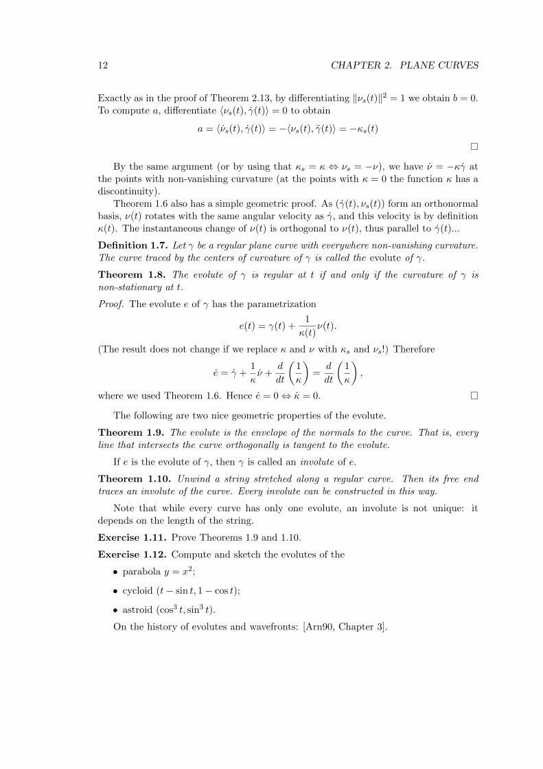
Definition 1.7. Let γ be a regular plane curve with everywhere non-vanishing curvature.The curve traced by the centers of curvature of γ is called the evolute of γ.

Theorem 1.8. The evolute of γ is regular at t if and only if the curvature of γ isnon-stationary at t.

Proof. The evolute e of γ has the parametrization

e(t) = γ(t) +1

κ(t)ν(t).

(The result does not change if we replace κ and ν with κs and νs!) Therefore

e = γ +1

κν +

d

dt

(1

κ

)=

d

dt

(1

κ

),

where we used Theorem 1.6. Hence e = 0⇔ κ = 0.

The following are two nice geometric properties of the evolute.

Theorem 1.9. The evolute is the envelope of the normals to the curve. That is, everyline that intersects the curve orthogonally is tangent to the evolute.

If e is the evolute of γ, then γ is called an involute of e.

Theorem 1.10. Unwind a string stretched along a regular curve. Then its free endtraces an involute of the curve. Every involute can be constructed in this way.

Note that while every curve has only one evolute, an involute is not unique: itdepends on the length of the string.

Exercise 1.11. Prove Theorems 1.9 and 1.10.

Exercise 1.12. Compute and sketch the evolutes of the

• parabola y = x2;

• cycloid (t− sin t, 1− cos t);

• astroid (cos3 t, sin3 t).

On the history of evolutes and wavefronts: [Arn90, Chapter 3].


Figure 2.1: The evolute of an ellipse.

1.3 Parallel curves and wave fronts

Definition 1.13. Let γ : I → R2 be a regular curve, and νs : I → R2 be its signed unitnormal. Choose δ ∈ R The curve

γδ = γ + δνs

is called a parallel curve to γ at distance δ.

Theorem 1.14. Singular points of a curve parallel to γ are centers of curvature of γ.

Proof. We have

γδ = γ + δνs = (1− δκs)γ

(In particular, the velocity vector of γδ at t is parallel to the velocity vector of γ at t.This also implies that being parallel is a symmetric and transitive relation.) Thus γδ issingular at t if and only if δ = 1

κs(t). The corresponding point of γδ is

γδ(t) = γ(t) +1

κs(t)· νs(t),

which is the center of curvature of γ at t.

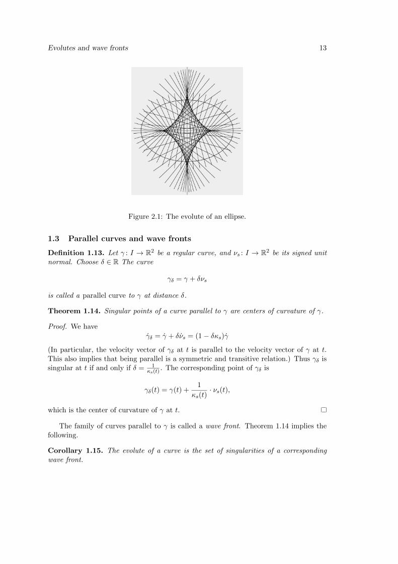
The family of curves parallel to γ is called a wave front. Theorem 1.14 implies thefollowing.

Corollary 1.15. The evolute of a curve is the set of singularities of a correspondingwave front.


Figure 2.2: The wave front of an ellipse.

See Figure 2.2.

Corollary 1.16. Parallel curves have the same evolutes.

Exercise 1.17. Show that the signed curvature of a parallel curve at non-singular pointsis equal to

κs1− δκs

1.4 Distance functions

Let γ : [a, b]→ R2 be a simple regular curve. For ε > 0 small enough, all parallel curvesγδ with |δ| < ε are also simple and pairwise disjoint:

γδ1(t1) = γδ2(t2)⇔ δ1 = δ2, t1 = t2

(we leave this fact without proof). The union of the images of all these curves is a tubularneighborhood of γ(I). Notation: Nε(γ).

A necessary (but not sufficient) condition for the images of γδ to be disjoint is ε < 1κ(t)

for all t.

Definition 1.18. Let p = γδ(t) ∈ Nε(γ). Then (t, δ) are called the normal coordinatesof p.

The coordinate lines t = const are straight line intervals intersecting γ orthogonally;the coordinate lines δ = const are curves parallel to γ.

Theorem 1.19. If ε > 0 is small enough, then the normal coordinate map δ : Nε(γ)→ Rassociates to every point its distance to γ(I):

p = γδ(t) ∈ Nε(γ)⇔ δ = minx∈γ(I)

‖p− x‖


The gradient of the map δ has norm 1 everywhere:

‖∇δ‖ = 1

Proof. If p = γδ(t) = γ(t) + δνs(t), then ‖p − γ(t)‖ = δ, thus δ(p) ≥ dist(p, γ). Onthe other hand, the circle of radius δ centered at p has with γ(I) only the point γ(t)in common. (Locally this follows from the fact that κ < 1

|δ| everywhere, and is relatedto the behaviour of osculating circles. Globally this can be ensured by an appropriatechoice of ε.) Hence δ(p) = dist(p, γ).

For every differentiable function F : R2 → R we have

‖∇F‖ = max‖v‖=1

∣∣∣∣∂F∂v∣∣∣∣

The derivative of δ in the direction of the oriented normal equals 1:

∂δ

∂ν(t)= 1.

Hence, ‖∇δ‖ ≥ 1. Assume there is a unit vector v such that∣∣ ∂δ∂v

∣∣ > 1. Then for asufficiently small α > 0 we have

δ(p+ αv) > δ(p) + α

On the other hand, by the triangle inequality we have dist(p + αv, γ) ≤ dist(p, γ) + α.This contradiction shows that all directional derivatives of δ are smaller than 1 in theabsolute value. Hence ‖∇δ‖ = 1.

The condition ‖∇F (p)‖ = 1 for all p is very strong.

Theorem 1.20. Let F : U → R be a function on a planar domain with ‖∇F (p)‖ = 1for all p ∈ U . Then locally the level sets of F are parallel curves.

This statement is only local because the domain U may not have the shape of atubular neighborhood.

First we need two lemmas about functions with gradient norm 1.

Lemma 1.21. Assume that ‖∇F‖ = 1 everywhere in a convex domain W . Then forany p, q ∈W we have

|F (p)− F (q)| ≤ ‖p− q‖

Proof. Let v = p−q‖p−q‖ be the unit vector pointing from q to p. Connect p to q by a

straight line segment l(t) = q + tv, t ∈ [0, ‖p− q‖]. Then we have

F (p)− F (q) =

∫ ‖p−q‖0

∂F

∂v(l(t)) dt

Since∣∣∂F∂v

∣∣ ≤ 1, the statement follows.


Lemma 1.22. Every gradient curve of a function F : U → R with ‖∇F‖ = 1 is astraight line.

A gradient curve of F is a curve λ such that λ(t) = ∇F (λ(t)) for all t. This is acurve that always follows the direction of the steepest ascent.

Proof. Let λ : [a, b]→ U be a gradient curve of F . By the chain rule we have

d

dtF (λ(t)) = 〈∇F, λ〉 = ‖∇F‖2 = 1.

Together with Lemma 1.21 this implies

‖λ(b)− λ(a)‖ ≥ |F (λ(b))− F (λ(a)) = b− a

On the other hand, the length of λ equals∫ b

a‖λ‖ dt = b− a

But the length of a curve does not exceed the distance between its endpoints, and if thelength is equal to distance, then this curve is a straight line.

Proof of Theorem 1.19. Since ∇F 6= 0, the level sets are regular curves. The linesperpendicular to the level curves are the gradient curves of F , by the lemma above.Since the restriction of F to each gradient curve measures the length of the curve (as‖∇F‖ = 1), moving along each normal by distance δ brings us to another level set of F .Hence the level sets are parallel curves.

Functions satisfying ‖∇F (p)‖ = 1 for all p are called distance functions.

2 Rotation index and convex curves

2.1 The total signed curvature

Smooth closed curve γ : [a, b]→ R2:

dkγ

dtk(a) =

dkγ

dtk(b) for all k ≥ 0

(if we only assume γ(a) = γ(b), then the curve may have a “knick”).Recall the definition of the function ϕ : [a, b]→ [0, 2π). Note that ϕ may be discon-

tinuous at the points where it takes value 0.

Lemma 2.1. There is a continuous map ϕ : I/ ∼→ R such that ϕ(t) ≡ ϕ(t)( mod 2π).

For this new function we have

κs =dϕ

dt

Rotation index and convex curves 17

Theorem 2.2. For every smooth closed curve its total signed curvature is an integermultiple of 2π: ∫

γκs dt = 2πι(γ), ι(γ) ∈ Z,

where t is the arc-length parameter on the curve.

The number ι(γ) is called the rotation index of γ.

Proof. We have ∫γκs dt =

∫ b

a

dϕ

dtdt = ϕ(b)− ϕ(a) = 2πk,

since ϕ(a) = ϕ(b) and ϕ differs from ϕ by an integer multiple of 2π.

2.2 Rotation of simple closed curves

Theorem 2.3. The rotation index of every simple smooth closed curve is equal to ±1.

Proof. Proof by H. Hopf [Hop35], see [Hsi97].

2.3 Convex curves

Definition 2.4. A curve is called convex, if it lies on one side of each of its tangentlines.

Lemma 2.5. The signed curvature of a convex curve does not change its sign.

Proof. Assume that κs is negative on (t0 − ε, t0) and positive on (t0, t0 + ε). Then thearc γt0t0−ε lies on the right of the oriented tangent at t0, and the arc γt0+ε

t0on the left of

this tangent. (Compare this with the behavior of the osculating circles.)

In general, the sign does not change at a point, but there is an interval (t0, t1) whereκ vanishes, and the signs before t0 and after t1 differ. In this case γt1t0 is a straight linesegment and short arcs before t0 and after t1 lie on different sides from this line.

In the following we assume that the curve does not “repeat itself” (like the doublecircle γ : [0, 4π)→ R2, γ(t) = (cos t, sin t)).

Theorem 2.6. Every convex curve is simple.

Proof. If the tangents at an intersection point differ, then each of them cuts the curve.If the tangents coincide, a tricky argument shows that the curve arcs must coincide in aneighborhood of the point. It follows that if a convex curve is not simple, it must repeatitself.

Theorem 2.7. The rotation index of a convex curve equals ±1.

Proof. Follows from Theorems 2.6 and 2.2.


2.4 Convex curves in polar coordinates

Radial graph r = r(t). Parametrization (r(t) cos t, r(t) sin t).Formulas for the arclength and the area.Among all curves of a given diameter the circle encloses the largest area (proof

mentioned in the Littlewood book).

3 Global geometry of plane curves

3.1 Support function

Definition 3.1. Let X ⊂ R2 be a compact set. A support line of X is an oriented linethat has at least one point in common with X and such that X lies on the left from thisline.

The support function of X associates to every unit vector v ∈ R2 the signed distancefrom the origin to the support line of X with the exterior normal v:

hX(v) = maxx∈X〈v, x〉

If X is a convex positively oriented curve, then all its support lines are its tangents,compatibly oriented.

We will consider only positively oriented convex curves. (Note that this is equivalentto the requirement κs ≥ 0.)

Definition 3.2. A smooth convex curve is called strictly convex, if it has only one pointin common with each of its tangents.

Exercise 3.3. Show that κs > 0 implies strict convexity, but is not vice versa.

Strictly convex curves have a special parametrization: to every unit vector we canassociate the point that has this vector as the exterior unit normal.

Definition 3.4. The Gauss parametrization of a smooth strictly convex curve is a map

γ : [0, 2π)→ R2

such that the exterior unit normal at t has direction t.

Note that the exterior unit normal is always opposite to the signed unit normal.We now modify our definition of the support function and denote by h(t) the value

at the vector (cos t, sin t).

Theorem 3.5. The Gauss parametrization of a smooth strictly convex curve is relatedto the support function by the formula

γ(t) = h

(cos tsin t

)+ h

(− sin tcos t

)

Global geometry of plane curves 19

Proof. Denote v(t) = (cos t, sin t) and w(t) = (− sin t, cos t). This is an orthonormalbasis, and v = w. Let γ(t) = a(t)v(t) + b(t)w(t). Use 〈γ(t), v(t)〉 = h(t). First, thisimplies a(t) = h(t). Second, its differentiation yields

〈γ, v〉+ 〈γ, v〉 = h

The first term vanishes, since the normal is orthogonal to the tangent. Hence b(t) =〈γ, v〉 = h.

3.2 The average width

Define the width of a compact set X in the direction of a unit vector v as the distancebetween the support lines with normals v and −v. In terms of the support function:

WX(v) = h(v) + h(−v)

Equivalently, the width in direction v is the length of the projection to the line parallelto v.

Again, we will use t as the argument of the width function.

Theorem 3.6 (Cauchy-Crofton formula). The length of a convex closed curve is pro-portional to the integral of its projection lengths:

L(γ) =1

2

∫ 2π

0Wγ(t) dt

Corollary 3.7. All figures of constant width W have perimeter πW .

Corollary 3.8. The average width of a convex closed curve is proportional to its length:

1

2π

∫ 2π

0Wγ(t) dt =

1

πL(γ)

The formula holds for non-smooth convex curves as well, because they can be ap-proximated by smooth convex ones.

Exercise 3.9. Find the average width of the unit square.

Proof of Theorem 3.6. Compute the length using the Gauss parametrization. First weneed to compute the norm of the velocity vector. We have

γ = h · v + h · v + h · w + h · w = (h+ h)w

because w = v. Since v looks left both from γ and from w, we have h + h > 0, so that‖γ‖ = h+ h.

L(γ) =

∫ 2π

0(h+ h) dt =

∫ 2π

0h dt =

1

2

∫ 2π

0(h(t) + h(−t)) dt


For convex polygons the Cauchy-Crofton formula can be proved by a different elegantargument.

Exercise 3.10. Prove directly that the length of a segment is quarter of its averagewidth. Derive the Cauchy-Crofton formula for convex polygons.

3.3 Isoperimetric inequality

Theorem 3.11. Among all simple closed curves of given length the circle bounds thelargest area. In other words, if A is the area bounded by a simple closed curve γ of lengthL, then

L2 − 4πA ≥ 0,

and the equality holds only if γ is a circle.

We will prove the isoperimetric inequality under assumption that γ is a smoothconvex curve.

Lemma 3.12. The area of a smooth convex curve with support function h is given by

A =1

2

∫ 2π

0(h2 − (h)2) dt

Proof. In the Gauss parametrization we have

γ = hv + hw, γ = (h+ h)w

Hence

γ × γ = h(h+ h)

It follows that

A =1

2

∫ 2π

0(h2 + hh) dt =

1

2

∫ 2π

0(h2 − (h)2) dt,

where integration by parts was used.

Lemma 3.13 (Wirtinger). Let f : [0, 2π)→ R be a smooth function with zero average:∫ 2π

0f dt = 0

Then ∫ 2π

0f2 dt ≤

∫ 2π

0(f)2 dt,

where the equality holds if and only if f(t) = a cos t+ b sin t for some a, b ∈ R.


Proof. Wirtinger’s inequality can be reformulated as a statement about the eigenvaluesof the Laplace operator. We have∫ 2π

0(f)2 dt = −

∫ 2π

0f · f dt = −〈∆f, f〉L2

The assumption∫ 2π

0 f dt = 0 means that f is L2-orthogonal to the space of constantfunctions, the kernel of the Laplace operator. Since the non-zero eigenvalues of ∆ are−n2, n ∈ Z (Fourier expansion of f), we have

−〈∆f, f〉L2 ≥ ‖f‖2L2 ,

which proves the inequality. The equality takes place if and only if f belongs to the(−1)-eigenspace, that is f(t) = a cos t+ b sin t.

Proof of Theorem 3.11. Let h be the support function of the curve γ. By scaling we canachieve L = 2π, that is

∫ 2π0 h dt = 2π. Put f(t) = h(t)−1. Then L = 2π ⇒

∫ 2π0 f dt = 0.

Hence Wirtinger’s lemma implies

A =1

2

∫ 2π

0(h2 − h2) dt =

1

2

∫ 2π

0(f2 − f2) dt+

∫ 2π

0f dt+ π ≤ π

Equality holds if and only if h(t) = 1 + a cos t+ b sin t, which is the support function ofthe unit circle centered at (a, b).

3.4 Steiner formulas

Let γ be a smooth closed convex curve, and δ > 0. The parallel curve γ−δ lies in theexterior of γ, and we will call it the exterior parallel curve.

Lemma 3.14. If h is the support function of γ, then the support function of the exteriorparallel curve at distance δ equals h+ δ.

Proof. If the maximum of 〈x, v〉 is attained at x = γ(t), then v is the exterior unitnormal of γ at t. Then γ(t)+δv is a point on the parallel curve, and it can easily be seenthat it realizes the maximum of the scalar product with v over the parallel curve.

Theorem 3.15. Let L and A be the length and the area of a smooth closed convex curveγ. Then the length and the area enclosed by the exterior parallel curve at distance δ areequal

Lδ = L+ 2πδ, Aδ = A+ Lδ + πδ2

Proof. Using the lemma above and the formulas for the length and area in terms of thesupport function we compute

Lδ =

∫ 2π

0(h+ δ) dt = L+ 2πδ

Aδ =1

2

∫ 2π

0

((h+ δ)2 − (h)2

)dt = A+ δ

∫ 2π

0h dt+

δ2

2

∫ 2π

0dt = A+ Lδ + πδ2


Exercise 3.16. Prove Steiner formulas for convex polygons.

3.5 Gauss map

The Gauss parametrization of a smooth convex closed curve can be viewed as a mapS1 → C ⊂ R2. Its inverse is called the Gauss map.

In fact, while the Gauss parametrization is defined only for strictly convex curves,the Gauss map makes sense for non-strictly convex curves as well.

Definition 3.17. Let C ⊂ R2 be a smooth convex closed curve. The Gauss map

Γ: C → S1

associates to every point p ∈ C the exterior unit normal to C at p.

Theorem 3.18. The Jacobian of the Gauss map is equal to the absolute curvature ofthe curve.

Here by the Jacobian we mean the length scaling factor. Both C and S1 are equippedwith a measure (the angular measure on S1 and the ‖γ‖dt measure on C, which isindependent of the parametrization γ). The measure of the Gauss image of an arcdivided by the measure of the arc tends to a limit as the arc length tends to zero.

Proof. This is a reformulation of Theorem 1.4:

dϕ

d`= κs ⇒

∣∣∣∣dϕd`∣∣∣∣ = κ

Here we denote by ` an arc-length parameter on C.

As a consequence, the integral of any function over curve C can be rewritten as theintegral over S1: ∫

Cf d` =

∫ 2π

0fκ−1 dt

For example, the total curvature of a convex curve can now be computed as∫Cκ d` =

∫ 2π

0dt = 2π

Theorem 3.19. The radius of curvature of a smooth convex closed curve can be com-puted from its support function by the formula

R = h+ h

Proof. Indeed, as we found out in the proof of Theorem 3.6, the Jacobian of the Gaussparametrization equals h + h. Since the Jacobian of the inverse is the inverse of theJacobian, and the radius of curvature is the inverse of the curvature, Theorem 3.18implies R = h+ h.


3.6 Minkowski formulas

Theorem 3.20. For every smooth convex closed curve C ⊂ R2 the following identitieshold: ∫

Cκν d` = 0,

∫Cν d` = 0

Proof. Use the Gauss parametrization of C. Then the identities become∫ 2π

0v(t) dt = 0,

∫ 2π

0κ−1(t)v(t) dt = 0

The first one is obvious. For the second one remember that κ−1 = h + h and applyintegration by parts: ∫ 2π

0hv dt = −

∫ 2π

0hv dt =

∫ 2π

0hv dt

Since v = −v, the result follows.

Remark 3.21. The second Minkowski formula has a physical interpretation. It saysthat the vector of the total pressure exerted on the perimeter of a planar balloon is azero vector.

3.7 Four-vertex theorem

Definition 3.22. A vertex of a smooth curve is a point of a local extremum of thecurvature.

An ellipse has four vertices. A circle has infinitely many.

Theorem 3.23 (Four-vertex theorem). Every simple closed smooth curve has at leastfour vertices.

Note that the simplicity assumption is essential. There are non-simple closed curveswith only two vertices (one is the global minimum, the other is the global maximum ofcurvature).

We will prove the four-vertex theorem for convex curves only.

Lemma 3.24. For every smooth convex closed curve parametrized with the unit speedthe following identity holds: ∫

Iκγ dt = 0,

Proof. Apply integration by parts:∫Iκγ dt = −

∫Iκγ dt = 0

The last integral is equal to zero since∫I κν dt = 0 by the first Minkowski formula,

and because the unit tangent vector γ is obtained by 90◦-rotation from the unit normalν.


Proof of the four vertex theorem. The above lemma implies that for every vector c ∈ R2

we have ∫Iκ〈γ, c〉 dt = 0 (2.1)

Assume the contrary: there is a curve that has only two vertices P (the globalmaximum of the curvature) and Q (the global minimum of the curvature). The line PQcuts the curve in two arcs ~PQ and ~QP . Choose the coordinate origin on the line PQand a vector c orthogonal to PQ and looking towards the arc ~QP . Then on the arc ~QPwe have κ ≥ 0 and 〈γ, c〉 > 0, and on the arc ~PQ we have κ ≤ 0 and 〈γ, c〉 < 0. It followsthat the integrand in (2.1) is everywhere non-negative (and somewhere positive), whichis a contradiction.

An alternative proof of the four-vertex theorem is based on the following.

Theorem 3.25 (Sturm). A periodic function free of the harmonics of order < k changesthe sign at least 2k times.

Indeed, the radius of curvature in terms of the support function h + h contains noharmonics of order 1; hence its derivative contains no harmonics of order < 2. Sturmtheorem implies that the derivative of the curvature changes the sign at least four times,hence the curvature has at least four extrema.

The proof of the Sturm theorem is based on the same idea as the above proof ofthe four-vertex theorem. If a function changes its sign at most 2k − 2 times, then thereis a trigonometric polynomial of degree < k that changes its sign at the same points.Then the L2-product of the function and the polynomial is positive; on the other hand afunction without harmonics of order < k is L2-orthogonal to trigonometric polynomialsof degree < k.

3.8 Steiner point

Definition 3.26. The Steiner point of a smooth convex closed curve is defined by meansof the Gauss parametrization as

St(γ) =1

π

∫ 2π

0h(t)v(t) dt

where, as usual, v(t) = (cos t, sin t).

Don’t confuse it with other points (associated to triangles) also carrying the nameof Steiner!

Exercise 3.27. Show that the Steiner point is the center of mass for a mass distributedalong the curve with the density proportional to the curvature. Because of this theSteiner point is sometimes called the curvature centroid.

In particular, the Steiner point is equivariant with respect to rigid motions: if a curveis translated or rotated, its Steiner point is subject to the same transformation.


Exercise 3.28. Show that the Steiner point possesses the following extremal property.Roll the curve along a straight line. For every point inside the curve consider its (pe-riodic) trajectory and the area under (a period of) this trajectory. The Steiner pointminimizes this area.

This is the original definition given by Steiner [Ste40].

Chapter 3

Space curves

1 Torsion

1.1 Frenet formulas

Suppose we have a space curve γ : I → R3 with nowhere vanishing curvature. Thismeans that, if γ is of unit-speed (which we assume in this section), then

γ = κν 6= 0

The vectors γ and ν can be completed to a positively oriented orthonormal basis

e1(t) = γ, e2(t) = ν, e3(t) = e1(t)× e2(t)

Definition 1.1. The vectors e1(t), e2(t), e3(t) (the unit tangent, the normal, and thebinormal) applied to the point γ(t) form a moving frame, called the Frenet frame of thecurve γ.

Let us compute the change of the vectors ei(t) as the point moves along the curve.We already know

e1 = κe2

Determine now the coefficients in

e2 = ae1 + be3, e3 = ce1 + de2

(recall that 〈e2, e2〉 = 0 because of ‖e2(t)‖ = 1). We have

a = 〈e2, e1〉 = −〈e2, e1〉 = −κ

Definition 1.2. The coefficient at e3 in the decomposition of e2 with respect to theFrenet frame is called the torsion of the curve γ:

e2 = −κe1 + τe3

26

Torsion 27

Further, we computec = 〈e3, e1〉 = −〈e3, e1〉 = 0

d = 〈e3, e2〉 = −〈e3, e2〉 = −τ

Altogether, the formulase1 = κe2

e2 = −κe1 + τe3

e3 = −τe2

are called the Frenet formulas.

Remark 1.3. The Frenet formulas can be written ase1

e2

e3

=

0 κ 0−κ 0 τ0 −τ 0

e1

e2

e3

The 3 × 3-matrix in this formula is skew-symmetric. This holds for any moving frameand is due to the fact that the skew-symmetric matrices form the tangent space to theorthogonal group at the point id.

Example 1.4. The curvature and the torsion of the circular helix

γ(t) = (a cos t, a sin t, bt)

1.2 Osculating plane and osculating sphere

The plane spanned by the tangent and the normal of a curve γ at the point t0 is calledthe osculating plane at t0. This is the plane that is the closest to γ in a neighborhoodof t0. To find how close it is, let us consider the Taylor expansion of γ near t0.

Theorem 1.5. Assume that γ(0) = 0 and put κ0 = κ(0), τ0 = τ(0). Then the coordi-nates of γ(t) in the Frenet frame of the point γ(0) have the form

x1(t) = t− κ20

6t3 + o(t3)

x2(t) =κ0

2t2 +

κ′(0)

6t3 + o(t3)

x3(t) =κ0τ0

6t3 + o(t3)

Projections of the curve to the planes spanned by the Frenet basis vectors (in thecase κ0 6= 0, τ0 6= 0).

If κ0 6= 0 and τ0 6= 0, then the osculating plane cuts the curve locally in two parts.The tangent line approximates the curve up to terms of order 2 (the t2 term vanishes

if κ = 0). The osculating circle approximates the curve up to terms of order 3 (whendoes the t3 term vanish?). The osculating plane approximates the curve up to terms oforder 3 (the t3 vanishes if κτ = 0).

28 CHAPTER 3. SPACE CURVES

Definition 1.6. The osculating sphere of the curve γ at the point γ(t) is the sphere thatapproximates γ near t up to terms of order 4 at least.

Theorem 1.7. The center of the osculating sphere at the point γ(t) is the point γ(t) +1κ(t)e2(t) + 1

τ(t)

(1κ(t)

)·e3(t).

Proof. Substitute the formulas of Theorem 1.5 into the equation of the sphere withcenter (a1, a2, a3) passing through the origin:

x21 + x2

2 + x23 − 2a1x1 − 2a2x2 − 2a3x3 = 0

The requirement that the coefficients at t, t2, and t3 vanish yields a system of linearequations on a1, a2, a3. By solving it we obtain the coordinates of the center of theosculating sphere with respect to the Frenet frame

(0, 1

τ ,1κ

(1τ

)·).

Exercise 1.8. Let c(t) be the curve formed by the centers of the osculating spheres.

1. Show that the tangent to c at t is parallel to the binormal of γ at t. (Comparethis with the situation in the plane, where the tangents to the evolute are parallelto the normals of the curve.)

2. Show that the singular points of c correspond to the points of γ where

τ

κ+

(1

τ

(1

κ

)·)·= 0 (3.1)

3. Show that the curve γ lies on a sphere if and only if the above equation holdseverywhere on γ.

1.3 Existence and uniqueness theorems

The initial position of the Frenet frame, the curvature (non-vanishing), and the torsion,both given as functions of the arclength, determine the curve uniquely.

2 Global geometry of space curves

2.1 Curves on the sphere

The result of the last exercise immediately implies that for every closed space curvecontained in a sphere we have ∫

γ

τ

κd` = 0

There is a more elegant vanishing theorem.

Theorem 2.1 (Geppert). The total torsion of every closed spherical curve equals zero:∫γτ d` = 0

Global geometry of space curves 29

In order to prove this, let us look at the spherical curves more closely. It suffices tostudy the curves on the unit sphere centered at the origin: ‖γ(t)‖ = 1 for all t. Introducethe notation e0(t) = γ(t). In addition to the Frenet formulas we then have e0 = e1.

Lemma 2.2. The curvature of a curve on the unit sphere is at least 1.

Proof. We have κ = ‖e1‖ = ‖e0‖. On the other hand,

0 = 〈e0, e0〉· = 1 + 〈e0, e0〉

Therefore

κ = ‖e0‖ ≥ |〈e0, e0〉| = 1

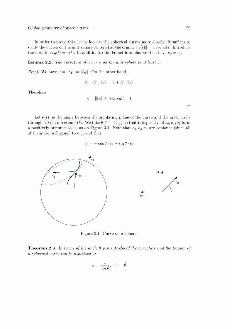
Let θ(t) be the angle between the osculating plane of the curve and the great circlethrough γ(t) in direction γ(t). We take θ ∈ (−π

2 ,π2 ) so that it is positive if e0, e1, e2 form

a positively oriented basis, as on Figure 3.1. Note that e0, e2, e3 are coplanar (since allof them are orthogonal to e1), and that

e0 = − cos θ · e2 + sin θ · e3

e0

e1

e2

e2

e0

e3

θ

Figure 3.1: Curve on a sphere.

Theorem 2.3. In terms of the angle θ just introduced the curvature and the torsion ofa spherical curve can be expressed as

κ =1

cos θ, τ = θ


Proof. From the argument in the previous lemma and from e1 = κe2 we have

−1 = 〈e0, e1〉 = κ〈e0, e2〉 = −κ cos θ

Further, by differentiating the equation − cos θ = 〈e0, e2〉 we obtain

θ sin θ = 〈e0, e2〉+ 〈e0, e2〉 = 〈e0,−κe1 + τe3〉 = τ sin θ

Now we can reprove the first theorem of this section and prove Geppert’s theorem:∫C

τ

κd` =

∫ L

0θ cos θ dt =

∫ L

0(sin θ)· dt = 0

∫Cτ d` =

∫ L

0θ dt = 0

Also, it follows that κ = 1cosθ, τ = θ provides a general solution of the differential equation

(3.1).Interestingly enough, the torsion is the speed of the binormal indicatrix, which is

itself a spherical curve. The binormal indicatrix is the spherical analog of the evolute.Thus, Geppert’s theorem is a spherical analog of the fact that the signed length of theevolute vanishes.

The dual curves (?).For more about curves on the sphere see [Arn95].

2.2 Fenchel theorem

Theorem 2.4 (Fenchel). The total curvature of a space curve does not exceed 2π. Itequals 2π only for convex plane curves.

As a preparation for the proof, we will need a definition, two lemmas, and a theorem.

Definition 2.5. Let γ be a unit-speed space curve. Then the curve on the unit spheretraced by the vector γ is called the tangent indicatrix of γ.

For example, if γ lies in a plane, its tangent indicatrix is contained in the great circleparallel to this plane. In this case the indicatrix will backtrack at the places where thesigned curvature changes its sign; it will be a simple curve if and only if γ is convex.

Lemma 2.6. The total curvature is the length of the tangent indicatrix.

Proof. Indeed, ∫Cκ dt =

∫ L

0‖γ‖ dt =

∫ L

0‖e1‖ dt = L(e1)

and the curve e1 : [0, L]→ S2 is the tangent indicatrix.

Global geometry of space curves 31

Lemma 2.7. The tangent indicatrix intersects each great circle at least twice.

Proof. Every great circle can be represented as

v◦ = v⊥ ∩ S2

for some non-zero vector v ∈ R3. Now

e1(t) ∈ v◦ ⇔ 〈e1(t), v〉 = 0⇔ 〈γ(t), v〉· = 0

But the function t 7→ 〈γ(t), v〉 has at least two critical points: the global maximum andthe global minimum. Therefore the curve e1 intersects v◦ at least twice.

Theorem 2.8 (Crofton). Let C be a smooth curve of length L on the unit sphere.Let M be the measure of the oriented great circles intersecting C, each counted with amultiplicity which is the number of its points of intersection with C. Then

M = 4L

The measure on the set of oriented great circles is induced from the standard measureon the sphere through the bijection between oriented great circles and points on thesphere: to every equator there correspond two poles, and if the equator is oriented,there is a consistent way to choose one of these poles.

Proof. For a formal proof, see [Hsi97]. We explain here why the theorem holds for arcsof great circles.

An oriented great circle S intersects an arc pq if and only if its pole S◦ lies betweenthe polars p◦ and q◦ of p and q. The space between p◦ and q◦ consists of two “lunes”,each of the angle L, where L is the distance between p and q. The area of each lune is2L.

Compare this with the Cauchy-Crofton formula in the plane, which can be interpretedin terms of the measure of the set of lines intersecting a convex curve.

Proof of the Fenchel theorem. Since the tangent indicatrix intersects every oriented greatcircle at least twice, its length is at least 2π. Hence the total curvature is at least 2π.The equality takes place only if the tangent indicatrix is a great circles, traced withoutbacktracking. This means that γ is a convex plane curve.

2.3 Weyl tube formula

Theorem 2.9. Let γ be a simple curve of length L in R2 or R3. Then the volume ofthe tubular ε-neighborhood of γ equals{

2εL in the plane

πε2L in the space


An analog holds for curves in Rn with n > 3. The length is multiplied with thevolume of the ball of radius ε in Rn.

Proof. Parametrize the tubular neighborhood by the rectangle/cylinder and integratethe Jacobian.

In the 3-dimensional case the normal-binormal parametrization is well-defined andcontinuous only if the curvature does not vanish. In the general situation, however, onecan take a parametrization defined by any moving orthonormal frame (e1, e2, e3).

For convex curves in the plane, the Weyl tube formula also follows from the Steinerformula. Just subtract A−δ from Aδ.

Chapter 4

Surfaces: the first fundamentalform

1 Definitions and examples

1.1 What is a surface?

Similar to curves, there are three convenient ways to represent a surface in R3:

• as the graph of a function f : U → R with U ⊂ R2;

• as a level set F (x, y, z) = 0;

• as the image of a map σ : U → R3 with U ⊂ R2.

Again, the third way is the most flexible one. But we encounter difficulties whentrying to represent some topologically non-trivial surfaces. In the case of curves we couldrepresent a closed curve as the image of a, say, periodic map; in the case of surfaces itis hard to parametrize the sphere by a “good” map. This leads us to use a collection oflocal parametrizations in order to represent a surface.

For simplicity, we will avoid dealing with self-intersecting surfaces (although can laterallow self-intersections). The following definition explains, what an embedded surfacewithout boundary is.

Definition 1.1. A subset S ⊂ R3 is a surface if, for every point p ∈ S there is an openset W ⊂ R3 containing p and a homeomorphism Φ: W →W ′ onto an open subset of R3

such that W ′ ∩ R2 = Φ(W ∩ S).

Informally speaking, the map Φ “flattens out” the surface in a neighborhood of p.Note that we don’t require the set W ′ ∩ R2 to be connected.

Definition 1.2. Let U ⊂ R2 be an open subset, and σ : U → R3 be a continuous mapwhose image is contained in the surface S. The pair (U, σ) is called a local parametriza-tion of S or a surface patch.

33

34 CHAPTER 4. SURFACES: THE FIRST FUNDAMENTAL FORM

The definition of a surface implies that for every point on a surface there is a surfacepatch covering its neighborhood. One may suggest this as a “simplified” definition ofa surface: a subset S ⊂ R3 such that for every p ∈ S there is a neighborhood of p inS homeomorphic to an open subset of R2. But this is not equivalent to the definitiongiven above. Counterexample: Alexander’s horned sphere.

For smooth surfaces there is no such a problem, so we may use the weak definitionas well.

1.2 Examples

A collection of local parametrizations is called an atlas.

Example 1.3. Three atlases for the sphere.

• The spherical coordinates

(θ, ϕ) 7→ (cos θ cosϕ, cos θ sinϕ, sin θ)

allow to cover the unit sphere by the rectangle [−π/2, π/2] × [0, 2π]. However,this is not a homeomorphism (examine θ = ±π/2), and the rectangle is closed.We get a surface patch if we restrict the map to the open rectangle. This gives aparametrization of the sphere minus half of a great circle (a meridian). We cancomplete the atlas by appropriately rotating the mapped region so as to cover thecomplement of a great half-circle disjoint from the unmapped meridian.

• The stereographic projection

R2 → S2, (x, y) 7→(

2x

1 + x2 + y2,

2y

1 + x2 + y2,−1 + x2 + y2

1 + x2 + y2

)is a homeomorphism onto the complement of the northern pole (0, 0, 1). It can becompleted to an atlas by a projection onto the complement of the southern pole.

• The map

{(x, y) | x2 + y2 < 1} → S2, (x, y) 7→ (x, y,√

1− x2 − y2)

is a part of an atlas that consists of 6 local parametrizations.

Example 1.4. A surface of revolution is the surface obtained by rotating a plane curvearound a line lying in the same plane. If the curve and the line are disjoint, then we obtainan embedded surface. Local parametrizations can be computed from a parametrizationof the curve. If γ(t) = (f(t), 0, g(t)), then the surface consists of the points

σ(t, ϕ) = (f(t) cosϕ, f(t) sinϕ, g(t)),

and can be covered by two patches (0, 2π) × I and (−π, π) × I (assuming I is an openinterval and γ is a simple curve).

Measuring lengths and areas 35

Torus.

Exercise 1.5. It is easy to find an atlas of four maps on the torus. Does there exist anatlas of three maps?

Example 1.6. Quadric surfaces. Ellipsoid, hyperboloids of one and of two sheets,hyperbolic paraboloid.

Exercise 1.7. Show that the hyperboloid of one sheet x2+y2−z2 = 1 and the hyperbolicparaboloid x2 − y2 = z are doubly ruled, that is every point lies on two different linescontained in the surface.

1.3 Smooth surfaces

Up to now, we spoke about topological surfaces. For example, the boundary of a convexpolyhedron is a surface in the sense of our definition (find an atlas of 4 maps on thesurface of the tetrahedron).

Definition 1.8. A surface patch σ : U → R3 is called regular if it is smooth and thevectors σu and σv are linearly independent at all points (u, v) ∈ U .

A smooth surface is a surface that can be parametrized by regular surface patches.Reparametrizations and transition maps.Tangent space and normals.Confocal quadrics.

2 Measuring lengths and areas

This section closely follows Pressley [Pre10].

2.1 Lengths of curves on surfaces

Let σ : U → R3 be a regular surface patch. Any space curve within σ(U) is the image ofa curve within U :

γ(t) = σ(u(t), v(t)), t ∈ [a, b]

Using the known formula for the length of a space curve and the chain rule, we compute

‖γ‖2 = 〈σuu+ σvv, σuu+ σvv〉 = ‖σu‖2u2 + 2〈σu, σv〉uv + ‖σv‖2v2

L(γ) =

∫ b

a‖γ‖ dt =

∫ b

a

√Eu2 + 2Fuv +Gv2 dt,

whereE = ‖σu‖2, F = 〈σu, σv〉, G = ‖σv‖2

The expressionds2 = Edu2 + 2Fdudv +Gdv2

36 CHAPTER 4. SURFACES: THE FIRST FUNDAMENTAL FORM

is called the first fundamental form of the surface S with respect to the local parametriza-tion σ. This is a symmetric (0, 2)-tensor field (a modern notation would be Edu⊗ du+F (du⊗ dv + dv ⊗ du) +Gdv ⊗ du) on U . We will use the notation

Iσ(X,Y ) = Ex1x2 + F (x1y2 + x2y1) +Gy1y2 = X>(E FF G

)Y,

where X = (x1, x2), Y = (y1, y2) ∈ R2 = TU . To every point of U this associates apositive definite symmetric bilinear form, which is the scalar product in R3 composedwith the linear map dσ:

Iσ(X,Y ) = 〈dσ(X), dσ(Y )〉

Example 2.1. • The first fundamental form of the sphere in the spherical coordi-nates:

dθ2 + cos2 θdϕ2

• More generally, the surface of revolution (f(t) cosϕ, f(t) sinϕ, g(t)) generated by aunit-speed parametrized curve (f(t), g(t)) has (with respect to the usual parametriza-tion) the first fundamental form

dt2 + f(t)dϕ2

The first fundamental form changes under reparametrization σ = σ ◦ ϕ as follows:

Iσ(X,Y ) = 〈dσ(X), dσ(Y )〉 = I(dϕ(X), dϕ(Y ))

In other words, (E F

F G

)= J>

(E FF G

)J,

where J is the Jacobi matrix of the map ϕ.

2.2 Isometries

2.3 Conformal maps

2.4 Surface area

Chapter 5

Curvature of surfaces

1 The second fundamental form

1.1 Deviation from the tangent plane

Compute the distance of the surface from one of its tangent planes. Given a surfacepatch σ, take a point σ(u, v), denote by ν the unit normal at this point. Then

dist = 〈σ(u+ δu, v + δv)− σ(u, v), ν〉

From the Taylor expansion,

dist =1

2

(L(δu)2 + 2Mδuδv +N(δv)2

)+ o((δu)2 + (δv)2),

where

L = 〈σuu, ν〉, M = 〈σuv, ν〉, N = 〈σvv, ν〉

The expression

IIσ = Ldu2 + 2Mdudv +Ndv2

is called the second fundamental form of the surface with respect to a local parametriza-tion σ.

Lemma 1.1. We have

IIσ(X,Y ) = −〈dσ(X), dν(Y )〉 = −〈dσ(Y ), dν(X)〉

Proof. We have to show that

L = −〈σu, νu〉, M = −〈σu, νv〉 = −〈σv, νu〉, N = −〈σv, νv〉

But this follows from differentiating the identities 〈σu, ν〉 = 0 = 〈σv, ν〉.

37

38 CHAPTER 5. CURVATURE OF SURFACES

Lemma 1.2. Let σ = σ ◦ ϕ be a reparametrization of the surface, and let Jϕ be theJacobi matrix of ϕ. Then (

L M

M N

)= ±J>

(L MM N

)J,

where we take the plus sign if det Jϕ > 0, and the minus sign if det Jϕ < 0.

Example 1.3. Compute the first fundamental form of a surface of revolution

σ(t, ϕ) = (f(t) cosϕ, f(t) sinϕ, g(t))

under assumption that the profile curve is unit-speed parametrized: (f)2 + (g)2 = 1.We obtain

IIσ = (f g − f g)dt2 + fgdϕ2

In particular, if (f(t), g(t)) = (1, t) (the surface is a cylinder), then IIσ = dϕ2. If(f(t), g(t)) = (cos t, sin t) (the surface is a unit sphere), then IIσ = dt2 + cos2 tdϕ2 = Iσ.

1.2 The curvature of curves on a surface

Let γ(t) = σ(u(t), v(t)) be a unit-speed curve on the surface. The velocity vector γ liesin the tangent plane. The acceleration vector γ is orthogonal to γ but not necessarilyorthogonal to the tangent plane. Let us decompose it into a normal and a tangentialcomponent. It is convenient to use the orthonormal frame (ν, γ, ν× γ). The accelerationvector will lie in the plane spanned by ν and ν × γ.

Definition 1.4. Let

γ = κnν + κg(ν × γ).

Then κn is called the normal curvature, and κg is called the geodesic curvature of γ.

Note that the absolute curvature of γ is given by

κ = ‖γ‖ =√κ2n + κ2

g

Lemma 1.5. The normal curvature of a unit-speed curve on a surface is given by

κn = Lu2 + 2Muv +Nv2 = IIσ(γ, γ)

Proof. From the definition of κn, we have

κn = 〈γ, ν〉 =

⟨ν,d

dt(σuu+ σvv)

⟩= 〈ν, σuu+ σvv + (σuuu+ σuvv)u+ (σvuu+ σvvv)v〉 = Lu2 + 2Muv +Nv2

Principal curvatures 39

Thus, the normal curvature of a curve on a surface depends only on the tangentvector of the curve, that is on the first-order data.

Theorem 1.6 (Meusnier). The curvature of a curve on a surface depends only on theosculating plane of the curve. Namely, if θ is the angle between the osculating plane ofthe curve and the tangent plane of the surface, then

κ sin θ = κn.

In other words, the osculating circles of all curves with the same tangent form a sphere(whose radius is the inverse of the normal curvature in the direction of the tangent).

Proof. The angle between the normal to the surface and the acceleration vector equalsπ2 − θ. Hence

κn = 〈γ, ν〉 = ‖γ‖‖ν‖ cos(π

2− θ) = κ sin θ.

Compare this with a particular case of curves on the unit sphere.Investigate what happens on a surface of revolution, if the tangent line is orthogonal

to the rotation axis.

2 Principal curvatures

2.1 Definition

Definition 2.1. The principal curvatures of a surface patch σ are the roots of theequation

det(IIσ − κIσ) = 0

Reparametrization does not change the principal curvatures.The roots are real (principal axes theorem).

2.2 Curvature of surfaces of revolution

The principal directions and principal curvatures of a surface of revolution.

2.3 Curvature lines and triply orthogonal systems

2.4 The shape operator and the Weingarten matrix

Definition 2.2. The shape operator

S : TpM → TpM, S(X) = −∇Xν

The eigenvectors and the eigenvalues of the shape operator are the principal curvaturedirections and the principal curvatures.


3 The Gaussian curvature and the mean curvature

3.1 Definitions and formulas

3.2 The third fundamental form

3.3 The Gauss map and the Gauss-Bonnet theorem for convex surfaces

3.4 Covariant differentiation

Definition 3.1. Let f : M → R. The gradient of f at p ∈M is a vector ∇Mf(p) ∈ TpMsuch that

∂f

∂X(p) = 〈∇Mf(p), X〉 for all X ∈ TpM

Lemma 3.2. For any smooth extension f : R3 → R of the function f we have

∇Mf(p) = >(∇f).

Here > : R3 → TpM is the orthogonal projection; it produces the tangential componentof a vector:

>(Y ) = Y − 〈Y, ν〉ν

Definition 3.3. Let Y : M → R3 be a vector field along the surface M , and let X ∈ TpM .The covariant derivative of Y in the direction X is

∇MX Y = >(∇X Y ).

On the right hand side we are taking the componentwise directional derivative of anarbitrary smooth extension Y of Y to R3.

Lemma 3.4. The following Leibniz-type formulas hold:

∇MX (fY ) = (∇MX f)Y + f · ∇MX Y∇MX 〈Y,Z〉 = 〈∇MX Y,Z〉+ 〈Y,∇MX Z〉

Theorem 3.5. The covariant differentiation and the second fundamental form are re-lated through the following formula:

∇MX Y = ∇XY − II(X,Y ) · ν

Proof. By definition,

∇MX Y = ∇XY − 〈∇XY, ν〉ν

On the other hand,

〈∇XY, ν〉 = −〈∇Xν, Y 〉 = II(X,Y )

because of 〈Y, ν〉 = 0. The theorem follows.

The Gaussian curvature and the mean curvature 41

3.5 Hessian and Laplacian

Definition 3.6. The Hessian operator of a function f : M → R is defined as

HessM f(X) = ∇MX (∇f)

The Hessian quadratic form is defined as

HessM f(X,Y ) = 〈∇MX (∇f), Y 〉

Lemma 3.7. The Hessian quadratic form is symmetric: HessM f(X,Y ) = HessM f(Y,X).

The definition is motivated by the matrix of second derivatives of a function f : R3 →R. There we have

Hess f(X,Y ) = 〈∇X(∇f), Y 〉 = X>(D2f)Y,

where D2f =(

∂f2

∂xi∂xj

).

Theorem 3.8. The Hessian and the Laplacian on the surface are related to the shapeoperator and the mean curvature through the following formulas:

HessM f(X) = >(Hess f(X)) + fν · S(X)

∆Mf = ∆f − fνν + fν · 2H

Proof.

∇MX (∇Mf) = ∇X(∇Mf)− 〈∇X(∇Mf), ν〉ν= ∇X(∇f − 〈∇f, ν〉ν)− c1ν = ∇X∇f − 〈∇f, ν〉∇Xν − c2ν

Since the left hand side belongs to TpM , the c2ν summand on the right hand side is thenormal component of ∇X∇f . Thus we get

HessM f(X) = >(Hess f(X))− 〈∇f, ν〉∇Xν = >(Hess f(X)) +∇νf · S(X)

Taking the trace of both sides, we obtain

∆Mf = tr(> ◦Hess f) +∇νf · 2H

By computing the matrix of Hess f in an orthonormal basis (e1, e2, ν), one sees that

tr(> ◦Hess f) = fe1e1 + fe2e2 = tr(Hess f)− fνν

There are two special choices of a function f where the formulas of the above Theoremyield interesting results.


Corollary 3.9. Let f be the distance function from M . Then ∆f = 2H.

Proof. Indeed, since fM = 0, we have ∇Mf = 0, and hence ∆M = 0. Also we havefν = 1 and fνν = 0.

Corollary 3.10. Consider the vector-valued function i : M → R3, i(p) = p. The com-ponentwise Laplacian of i equals the unit normal scaled by twice the mean curvature:

∆M i = 2H · ν

Proof. Each component of i is the restriction to M of a linear function on R3. If f(x) =〈a, x〉, then we have

∇f = a, ∆f = 0, fν = 〈a, ν〉, fνν = 0

Hence ∆Mf = 〈a, 2Hν〉. It follows that the Laplacian of the components of i consists ofthe components of 2Hν.

4 Parallel surfaces

4.1 Curvature of parallel surfaces

Let M ⊂ R3 be an orientable smooth surface, and ν be a field of unit normals along M .By a parallel surface at distance δ ∈ R we mean

M δ = {p+ δν | p ∈M}

We will show that for δ small enough M δ is smooth and will compute its curvatures.Note that a parallel surface M δ comes together with a natural map M →M δ.

Theorem 4.1. 1. Let C = maxp{|κ1(p)|, |κ2(p)|} and assume that |δ| < 1C . Then

the surface M δ is smooth.

2. The vector ν(p) is a unit normal to M δ at the point p + δν. That is, the tangentplanes to M and M δ at corresponding points are parallel.

3. The principal curvature directions of M δ are parallel to the principal curvaturedirections of M at the corresponding point, and are given by

κδi =κi

1− δκi

Proof. Choose a surface patch σ : U →M compatibly oriented with ν (that is, the basis(σu, σv, ν) is positively oriented). This gives rise to a surface patch σδ = σ + δν of M δ,and we have

σδu = σu + δνu, σδv = σv + δνv

Since νu, νv ∈ TpM , this shows already that νδ = ν, provided that M δ is smooth.

Parallel surfaces 43

Now let σ be chosen so that σu(p) and σv(p) are principal directions at p (this canbe achieved by a linear change of variables). This means

νu = −κ1σu, νv = −κ2σv

at the point p. Therefore

σδu = (1− δκ1)σu, σδv = (1− δκ2)σv

Hence, if |δ| is smaller than the maximum curvature radius, then the map σδ is regular,and the smooth surface M δ has the same normals as M . This proves the first and thesecond part of the theorem.

For the third part, since νδu = νu, we have from the above

νδu = − κ1

1− δκ1σδu, νδv = − κ2

1− δκ2σδv

It follows that σu and σv are principal curvature directions, and the principal curvaturesare as stated in the theorem.

4.2 Delaunay surfaces

4.3 Weyl tube formula

Lemma 4.2. The area of a parallel surface at distance δ is given by

area(M δ) = area(M)− 2δ

∫MH darea +δ2

∫MK darea .

Here we assume that δ is small enough, so that M δ is a smooth surface.

Proof. By Theorem 4.1 we have

σδu × σδv = (1− δκ1)(1− δκ2)σu × σv = (1− 2δH + δ2K)σu × σv

Integrating over the parametrization domain U yields the stated formula.

The domain between the parallel surfaces M ε and M−ε is called a tubular neighbor-hood of M and denoted by Nε(M).

Theorem 4.3 (Weyl’s tube formula). The volume of the tubular ε-neighborhood of asmooth surface M equals

vol(Nε(M)) = 2ε area(M) +2

3ε3

∫MK darea


Proof. Consider the map

Φ: U × [−ε, ε]→ R3, Φ(u, v, δ) = σδ(u, v) = σ(u, v) + δν(u, v),

whose image is Nε(M). The Jacobi matrix of Φ is

(σu + δνu, σv + δνv, ν),

so that

det Φ = ‖(σu + tνu)× (σv + tνv)‖

It follows that

vol(Nε(M)) =

∫U×[−ε,ε]

‖σδu × σδv‖ dudvdδ =

∫ ε

−εarea(M δ) dδ

Integration of the formula from Lemma 4.2 yields the formula of this theorem.

4.4 Steiner formula

Let M ⊂ R3 be a smooth convex surface. Let ν be the interior unit normal field, so thatthe principal curvatures of M (and hence the mean curvature) are positive. Let ε > 0,and denote by M and M ε the bodies bounded by M , and the exterior parallel surfaceM−ε.

Theorem 4.4 (Steiner). The volume enclosed by a parallel surface is given by

vol(M ε) = vol(M) + ε area(M) + ε2

∫MH darea +

4π

3ε3

Proof. Similar to the proof of the Weyl tube formula we have

vol(M ε) = vol(M) +

∫ ε

0area(M−δ) dδ

Integrating the formula from Lemma 4.2 yields the result.

5 Differential geometry of convex bodies

5.1 The support function

Similarly to the case of curves in the plane, we define the support function of a setM ⊂ R3 as

h : R3 → R, h(v) = maxx∈M〈x, v〉

Clearly, h is positively homogeneous: h(λv) = λh(v) for λ ≥ 0. Therefore, the restrictionof h to the unit sphere S2 ⊂ R3 gives the full information about it. Also, if M is a strictly

Differential geometry of convex bodies 45

smooth convex body, then maxx∈M 〈x, v〉 is attained at the point with the unit normalpositively proportional to v. It follows that we can write

h(v) = 〈Γ−1(v/‖v‖), v〉, (5.1)

where Γ−1 : S2 →M is the inverse of the Gauss map.

However, it is often convenient to view h as a function on R3. Then it is subadditive:

h(v + w) ≤ h(v) + h(w),

which together with the positive homogeneity implies that h is convex.

Lemma 5.1. A strictly convex surface is determined by its support function. Moreover,the Gauss parametrization of the surface can be written in terms of the support functionas

Γ−1(v) = gradh(v), ‖v‖ = 1

Proof. Differentiate equation (5.1) in the direction of a vector X ∈ R3 using the short-hand notation Γ−1(v/‖v‖) = p(v):

∂h(v)

∂X= 〈∂p(v)

∂X, v〉+ 〈p(v), X〉 = 〈p(v), X〉,

because ∂p(v)∂X ∈ Tp(v)M and hence is orthogonal to v. It follows that gradh(v) = p(v) =

Γ−1(v) for ‖v‖ = 1.

Note that one can define the support function on any surface whose Gauss map isinjective. This holds, for example, for a sufficiently small neighborhood of any pointwith non-vanishing Gaussian curvature.

5.2 Volume in terms of the support function

Lemma 5.2. The volume of a body with smooth boundary is given by

vol(M) =1

3

∫Mh darea

Proof. Consider the function f : R3 → R, f(x) = ‖x‖22 . We have grad f(x) = x, and

∆f = 3. Therefore by the Stokes theorem we have

3 vol(M) =

∫M

∆f(x) darea =

∫M〈grad f(p), ν(p)〉 darea =

∫Mh(p) darea .

A similar method can be used to prove one of the Minkowski formulas.


Theorem 5.3. For every body with smooth boundary M we have∫Mν(p) darea = 0

Proof. Consider this time a linear function f(x) = 〈a, x〉 on R3. We have grad f(x) = afor all x, and ∆f = 0. Therefore

0 =

∫M

∆f(x) darea =

∫M〈grad f(p), ν(p)〉 darea =

⟨a,

∫Mν(p) darea

⟩Since this holds for any a ∈ R3, it follows that the integral vanishes.

A physical interpretation: the total pressure on the surface of a balloon is a zerovector.

5.3 Minkowski formulas

Theorem 5.4. For every smooth convex surface M the following holds:

area(M) =

∫MhH darea,

∫MH darea =

∫MhK darea

Proof.

vol(M ε) =1

3

∫Mε

hε darea =1

3

∫M

(h+ ε)(1 + εκ1)(1 + εκ2) darea

=1

3

∫M

(h+ ε+ εh(κ1 + κ2) + ε2(κ1 + κ2) + ε2hκ1κ2 + ε3κ1κ2

)darea

= vol(M)+ε

3area(M)+

2ε

3

∫MhH darea +

2ε2

3

∫MH darea +

ε2

3

∫MhK darea +

ε3

34π

Comparing this with the Steiner formula for vol(M ε) we obtain the formulas of thetheorem.

Corollary 5.5. The average width of a convex body with smooth boundary is 12π of the

total mean curvature of its boundary:

1

4π

∫S2wv(M) darea =

1

2π

∫MH darea,

where wv(M) = hv(M) + h−v(M) is the width of M in the direction v.

Proof. Rewrite the first integral using the Gauss parametrization of M :

1

2π

∫S2h(v) darea =

1

2π

∫MhK darea

and apply the second Minkowski formula.

Minimal surfaces 47

5.4 Spherical harmonics

5.5 Spherical Laplacian and the Poincare-Wirtinger inequality

5.6 Support function and curvature

5.7 On the isoperimetric inequality

6 Minimal surfaces

6.1 Divergence, rate of the volume change, and the mean curvature

Let X : R3 → R3 be a vector field in R3. The divergence of X is defined as

divX = tr∇X =

3∑i=1

∂Xi

∂xi

For every vector field there is an associated flow ϕt : R3 → R3, ϕ0 = id, dϕt(p)dt =

X(ϕt(p)).

Lemma 6.1. The divergence of a vector field is equal to the rate of volume change underthe flow associated to the vector field:

divX(p) =d

dt

∣∣∣∣t=0

det dϕt(p)

Proof. We have

ϕt(p) = p+ tX(p) + o(t)

Therefore

dϕt(p) = id +t∇X(p) + o(t),

which implies

det dϕt = 1 + t tr(∇X) + o(t),

and the lemma is proved.

Remark 6.2. Instead of the flow ϕt in the above lemma one can take any smooth family

of diffeomorphisms ϕt such that dϕt(p)dt

∣∣∣t=0

(p) = X(p).

Now let M ⊂ R3 be a smooth surface, and ϕt : M → R3 a smooth family of smoothmaps such that ϕ0(p) = p for all p ∈M . Our goal is to determine how the area of ϕt(M)changes with t. The differential dϕt maps the plane TpM to the plane Tϕt(p)ϕt(M), andthe infinitesimal area change is equal to the determinant of this map (with respect tosome orthogonal bases in both planes). At the same time, this determinant is the squareroot of the Gram determinant √

det(dϕ>t dϕt).


It turns out that the infinitesimal rate of area change (that is the derivative of the abovedeterminant) can be expressed in terms of the divergence of the velocity vector field,this time the divergence with respect to the surface M .

The initial velocity of ϕt defines a vector field

X : M → R3, X(p) =dϕt(p)

dt

∣∣∣∣t=0

(p)

(which is not necessarily tangent to M). Define the divergence of X with respect to Mas

divM X = tr(∇MX) = 〈e1,∇Me1X〉+ 〈e2,∇Me2X〉where (e1, e2) is any orthonormal basis of TpM .

Lemma 6.3. For any smooth deformation of a surface the rate of the infinitesimal areachange is equal to the divergence of the initial velocity vector field along the surface:

d

dt

∣∣∣∣t=0

√det(dϕ>t dϕt) = divM X

Proof. As in the proof of the previous lemma, we have

dϕt(p) = id +t∇X(p) + o(t),

which implies that

dϕt(p)>dϕt(p) =

(δij + t(〈ei,∇ejX〉+ 〈ej ,∇eiX〉) + o(t)

)2i,j=1

Hence √det(dϕ>t dϕt) =

√1 + 2tdivM X + o(t) = 1 + tdivM X + o(t)

Theorem 6.4. The first variation of the area under a smooth deformation of a surfaceis given by

d

dt

∣∣∣∣t=0

area(ϕt(M)) = −2

∫MH〈X, ν〉 darea +

∫∂M〈X, ν∂M 〉 d`

Here ν∂M is the exterior unit normal to ∂M , tangent to M .

Proof. By Lemma 6.3 we have

d

dt

∣∣∣∣t=0

area(ϕt(M)) =

∫M

divM X darea =

∫M

divM (X>) darea +

∫M

divM (X⊥) darea,

whereX> andX⊥ are the tangential and the normal components ofX. For the tangentialcomponent we have∫

MdivM (X>) darea =

∫∂M〈X>, ν∂M 〉 darea =

∫∂M〈X, ν∂M 〉 darea,

and for the normal component X⊥ = fν we have

divM (fν) = 〈e1,∇e1(fν)〉+〈e2,∇e2(fν)〉 = f〈e1,∇e1ν〉+f〈e2,∇e2ν〉 = −f tr II = −2H〈X, ν〉

Minimal surfaces 49

6.2 Definition and examples of minimal surfaces

If we consider only deformations vanishing on ∂M , then

d

dt

∣∣∣∣t=0

area(ϕt(M)) = −2

∫MH〈X, ν〉 darea

It follows that H = 0 is a necessary and sufficient condition for the area of M to havezero derivative under all deformations vanishing on the boundary.

Definition 6.5. A surface M ⊂ R3 is called minimal, if its mean curvature vanisheseverywhere, that is, if M is a critical point of the area functional.

Example 6.6. The catenoid σ(t, θ) = (cosh t cos θ, cosh t sin θ, t). The Scherk surfacez = log cos y

cosx .

6.3 Conformal harmonic parametrizations

The following theorem gives an important characterization of minimal surfaces. In par-ticular, it will be used in finding the Weierstrass representation of minimal surfaces.

Theorem 6.7. If σ : U → R3 is conformal and (componentwise) harmonic, then σ(U)is a minimal surface. Conversely, every minimal surface can be locally parametrized byconformal harmonic surface patches.

Example 6.8. The Enneper minimal surface is

σ(u, v) =

(u− u3

3+ uv2, v − v3

3+ u2v, u2 − v2

)The components of σ are harmonic polynomials. Also we have

‖σu‖ = ‖σv‖ =√

1 + u2 + v2, 〈σu, σv〉 = 0

Thus σ is conformal and harmonic, and its image is a minimal surface.

A first approximation to Theorem 6.7 is the following

Lemma 6.9. A surface M ⊂ R3 is minimal if and only if the inclusion map i : M → R3

is harmonic: ∆M i = 0.

Proof. Follows directly from Corollary 3.10.

Two more lemmas are needed.

Lemma 6.10. Let σ : U →M be a conformal surface patch, and let f : M → R. Then

∆Mf = 0⇔ ∆(f ◦ σ) = 0.

This lemma will be proved in the next subsection.


Lemma 6.11. Every surface has an atlas consisting of conformal surface patches.

The proof is omitted.

Proof of Theorem 6.7. Assume that σ : U → R3 is conformal and componentwise har-monic: ∆(prα ◦σ) = 0 for α = 1, 2, 3. Put M = σ(U). By Lemma 6.10 we have∆M prα = 0. Hence by Lemma 6.9 the surface M has zero mean curvature.

In the opposite direction, assume M ⊂ R3 is minimal. Then, reversing the aboveargument, we see that every conformal surface patch of M is harmonic. By Lemma6.11 there is a conformal surface patch σ : U → M around every point. Thus M has aconformal harmonic atlas.

6.4 Laplacian and conformal maps

Our goal is to prove Lemma 6.10. Let ∆σ be an operator on C∞(U) corresponding tothe surface Laplacian:

∆σf = ∆M (f ◦ σ−1) ◦ f for every f : U → R

We want to show that for a conformal parametrization σ we have ∆f = 0⇔ ∆σf = 0.

Lemma 6.12. Let Iσ = λ(du2 + dv2). Then we have

∇σf = λ−1∇f

divσX = divX + λ−1 ∂λ

∂X

Proof. The first identity follows from

〈∇f,X〉 = Iσ(∇σf,X) = λ〈∇σf,X〉

for all X ∈ TpU = R2.

For the second one, note that the area element of Iσ is λ times the area element ofthe euclidean metric. Therefore the infinitesimal area change under ϕt with respect toIσ is

λ(ϕt(p))

λ(p)det dϕt

Theorem 6.13. If Iσ = λ(du2 + dv2), then

∆σf = λ−1∆f

Proof.

Minimal surfaces 51

6.5 Adjoint minimal surface

From Theorem 6.7 we know that every minimal surface has a conformal harmonicparametrization σ : U → R3. From now on we will assume that U is simply connected.

The harmonicity means that every component of

σ(u, v) = (x(u, v), y(u, v), z(u, v))

has zero Laplacian. Therefore the differential form xudv−xvdu is closed; by integratingit (here we use that U is simply-connected) we obtain a function x∗ : U → R such that

x∗u = −xv, x∗v = xu

It follows that x∗ is also harmonic; it is called the harmonic function conjugate to x.Note that x + ix∗ : U → C is a holomorphic function, with respect to the complex

coordinate u+ iv. We will return to the tools from the complex analysis later.

Definition 6.14. Let σ = (x, y, z) be a conformal harmonic parametrization of a min-imal surface. The map σ∗ : U → R3, σ∗ = (x∗, y∗, z∗), whose components are the har-monic functions conjugate to the components of σ, is called the adjoint of σ.

Theorem 6.15. Let σ∗ be the adjoint of a minimal surface σ. Then it has the followingproperties.

1. It is also a minimal surface.

2. The map σ(u, v) 7→ σ∗(u, v) is an isometry between the surface and its adjoint.

3. The tangent planes to σ(U) and σ∗(U) at the corresponding points are parallel.

Proof. The components of σ∗ are harmonic functions by construction. The first funda-mental form of σ∗ has the coefficients

‖σ∗u‖2 = ‖σv‖2 = ‖σu‖2 = ‖σ∗v‖2, 〈σ∗u, σ∗v〉 = −〈σv, σu〉 = 0,

hence σ∗ is conformal, hence σ∗(U) is a minimal surface.The above calculation of the coefficients of the first fundamental form shows that

σ(u, v) 7→ σ∗(u, v) is an isometry. Also obviously span{σ∗u, σ∗v} = span{σu, σv}.

Example 6.16. The adjoint of the catenoid

σ(u, v) = (coshu cos v, coshu sin v, u)

is the helicoidσ∗(u, v) = (sinhu sin v,− sinhu cos v, v)

Exercise 6.17. Find the adjoint of the Enneper surface

σ(u, v) =

(u− u3

3+ uv2, v − v3

3+ u2v, u2 − v2

)Show that the adjoint is actually congruent to the Enneper surface.


6.6 Associate family of minimal surfaces

Definition 6.18. Let σ : U → R3 be a conformal harmonic parametrization of a minimalsurface, and let σ∗ : U → R be its adjoint. The associate family of σ is the family ofmaps

σθ : U → R3, σθ = σ cos θ + σ∗ sin θ, θ ∈ [0, 2π)

In particular, σπ2

= σ∗.

Lemma 6.19. All surfaces of the associate family are minimal surfaces isometric to σ.Their tangent planes are parallel to the tangent planes to σ at the corresponding points.

Proof. It can be checked by a direct computation, using the already known propertiesof σ∗, that σθ is conformal and harmonic, and has the same first fundamental form asσ.

Alternatively, note thatσθ = Re(e−iθF ),

where F = σ + iσ∗. The components of e−iθF are holomorphic functions, therefore σθis harmonic. Conformality and isometry can be proved in a similar way, see the nextsection.

The tangent planes are parallel, because (σθ)u and (σθ)v are linear combinations ofσu, σv, σ

∗u = −σv, and σ∗v = σu.

6.7 Minimal surfaces and isotropic holomorphic curves in C3

The harmonicity of σ is equivalent to σ = Re(F ) for a holomorphic curve F : U → C3.How to express the conformality of σ in terms of F?

Extend the scalar product on R3 to a scalar product on C3:

〈z, w〉 = z1w1 + z2w2 + z3w3

(note: this is not the hermitian inner product!). If z = x + iy with x, y ∈ R3, then wehave

‖z‖2 = ‖x‖2 − ‖y‖2 + 2i〈x, y〉A vector z ∈ C3 is called isotropic, if ‖z‖2 = 0.

Lemma 6.20. A harmonic map σ : U → R3 is conformal if and only if the correspondingholomorphic curve

F = σ + iσ∗

has isotropic derivative:‖F ′‖2 = 0

Proof. We haveF ′ = σu − iσv

Hence‖F ′‖2 = 0⇔ ‖σu‖2 − ‖σv‖2 = 0 and 〈σu, σv〉 = 0

Minimal surfaces 53

Since U is simply connected, every holomorphic map F : U → C3 is a componentwiseintegral of a holomorphic map f : U → C3. Thus we arrive to the following conclusion.

Lemma 6.21. Let f = (f1, f2, f3) : U → C3 be an isotropic holomorphic curve: f21 +

f22 + f2

3 = 0. Then the map

σ(w) = σ0 + Re

∫ w

w0

f(w) dw, w = u+ iv, σ0 ∈ R3

determines a minimal surface, and

σ(w∗) = σ∗0 + Im

∫ w

w0

f(w) dw, σ∗0 ∈ R3

its adjoint. Conversely, every simply connected minimal surface has a parametrizationσ that arises from some isotropic holomorphic curve in this way.

6.8 Enneper-Weierstrass representation

There are different ways to solve the equation f21 +f2

2 +f23 = 0. For example, we can take

f1 and f2 to be arbitrary holomorphic functions and define f3 =√f2

1 + f22 (choosing

some branch of the square root). The following parametrization of the set of solutionshas a nice geometric meaning, as will be shown later.

Lemma 6.22. Let ϕ : U → C be a holomorphic function, and ψ : U → C ∪ {∞} be ameromorphic function such that ϕ 6≡ 0 and every point which is a pole of order n for ψis a zero of order ≥ 2n for ϕ. Then the functions

f1 =1

2ϕ(1− ψ2), f2 =

i

2ϕ(1 + ψ2), f3 = ϕψ

are holomorphic in U and satisfy f21 + f2

2 + f23 = 0. Conversely, every f = (f1, f2, f3)

such that f21 + f2

2 + f23 = 0, f 6≡ 0, f1 − if2 6≡ 0 can be written in this form.

Proof. The first part is obvious. For the second part, put

ϕ = f1 − if2, ψ =f3

f1 − if2.

Note that f1 = if2 would imply f3 = 0, so that the surface would lie in a plane.This yields the Enneper-Weierstrass representation of non-planar minimal surfaces.

Take any ϕ and ψ satisfying the above conditions and put

x(w) = x0 + Re

∫ w

w0

1

2ϕ(1− ψ2) dw

y(w) = y0 + Re

∫ w

w0

i

2ϕ(1 + ψ2) dw

z(w) = z0 + Re

∫ w

w0

ϕψ dw


Theorem 6.23. In the Enneper-Weierstrass representation the map ψ : U → C∪{0} isthe composition of the Gauss map with the stereographic projection:

ψ = π ◦ Γ ◦ σ, Uσ−→M

Γ−→ S2 π−→ C ∪ {0}

Proof. We have

σu − iσv = F =

(1

2ϕ(1− ψ2),

i

2ϕ(1 + ψ2), ϕψ

)From this we compute

Γ(σ(w)) =1

1 + |ψ|2(2 Reψ, 2 Imψ, |ψ|2 − 1)

Now the theorem follows from the formula for the inverse of the stereographic projection:

π−1(x, y) =1

1 + x2 + y2(2x, 2y, x2 + y2 − 1)

Chapter 6

Geodesics

1 Definition and variational properties

1.1 Curves of vanishing geodesic curvature

Let γ : I → M ⊂ R3 be a smooth curve on a smooth surface M . Decompose itsacceleration vector into the tangential and normal components:

γ = γ> + γ⊥.

By definition of the geodesic and normal curvatures (see Section 1.2, the geodesic cur-vature equals the norm of the tangential component of the acceleration vector:

κg = ‖γ>‖

Definition 1.1. A curve on a surface is called a (parametrized) geodesic, if its geodesiccurvature vanishes, that is, if its acceleration vector is orthogonal to the surface.

Also recall (although we will not need this) that if γ = cν, then c = II(γ, γ).

Lemma 1.2. Geodesics have constant speed.

Proof.d

dt‖γ‖2 = 2〈γ, γ〉 = 2〈γ, γ>〉 = 0

Let t = ϕ(s) be a parameter change along the geodesic. The curve γ = γ ◦ ϕ will becalled a reparametrized geodesic.

Lemma 1.3. A curve is a reparametrized geodesic if and only if the tangential componentof its acceleration vector is parallel to the velocity vector.

55

56 CHAPTER 6. GEODESICS

Proof. For a reparametrization ϕ of a curve γ we have

d2γ

ds2=d2ϕ

ds2γ +

(dϕ

ds

)2

γ.

Therefore, if γ is a geodesic, then the tangential component of γ vanishes, and the

tangential component of d2γds2

is parallel to dγds . Conversely, if the tangential component of

d2γds2

is parallel to dγds , then the function ψ = ϕ−1 can be found by solving the differential

equation of the formd2ψ

dt2· f +

(dψ

dt

)2

· g = 0.

Thus, you are moving along a geodesic if and only if your acceleration has only anormal component and a component collinear with the direction of your motion.

Note that the only reparametrizations of a geodesic that leave the acceleration vectororthogonal to the surface are the linear ones: s = ct, c = const.

In general, it is a difficult problem to describe geodesics on a surface explicitely (andwe will see in the next section, why). Below are some special cases, where we can assertthat a given curve is a geodesic.

Lemma 1.4. Any straight line segment on a surface is a geodesic.

Proof. Indeed, for a parametrization of the form γ(t) = a+bt we have γ = 0, in particularthe tangential component of γ is zero.

Lemma 1.5. Any normal section of a surface is a geodesic.

Proof. Let L ⊂ R3 be a plane orthogonal to M at every intersection point. Then L is theosculating plane of the intersection curve. It follows that for every parametrization γ ofthe intersection curve the acceleration vector γ is contained in L. Hence the tangentialcomponent of γ is parallel to γ, and γ is a reparametrized geodesic.

Example 1.6. The straight lines on the hyperboloid of one sheet and on the hyperbolicparaboloid are geodesics.

The meridians of surfaces of revolution are geodesics. The parallels at the criticalvalues of the radius are geodesics.

The big circles on the sphere are geodesics.

1.2 Geodesic equations and their consequences

Theorem 1.7. Let σ : U → M be a regular surface patch. A curve γ(t) = σ(u(t), v(t))is a geodesic if and only if the functions u(t) and v(t) satisfy a system of differentialequations

u+ P (u, v) = 0, v +Q(u, v) = 0,

where P and Q are symmetric bilinear forms whose coefficients depend on the coefficientsof the first fundamental form and their first derivatives.

Definition and variational properties 57

Lemma 1.8. A curve γ = σ(u(t), v(t)) is a geodesic if and only if

d

dt(Eu+ F v) =

1

2(Euu

2 + 2Fuuv +Guv2)

d

dt(Fu+Gv) =

1

2(Evu

2 + 2Fvuv +Gvv2)

Proof. By definition, γ is a geodesic if and only if the vector γ is orthogonal to M , thatis

〈γ, σu〉 = 0 = 〈γ, σv〉

We have

〈γ, σu〉 =d

dt〈γ, σu〉 −

⟨γ,

d

dtσu

⟩=

d

dt(uσu + vσv, σu)− 〈uσu + vσv, uσuu + vσuv〉

=d

dt(Eu+ F v)− (〈σu, σuu〉u2 + 〈σu, σuv〉uv + 〈σv, σuu〉uv + 〈σv, σuv〉v2)

On the other hand,

Eu =∂

∂u〈σu, σu〉 = 2〈σu, σuu〉

Fu =∂

∂u〈σu, σv〉 = 〈σuu, σv〉+ 〈σu, σuv〉

Gu =∂

∂u〈σv, σv〉 = 2〈σv, σuv〉

Substituting this into the above formula proves the first equation of the lemma. Thesecond equation is proved in a similar way.

Proof of the theorem. Transform the equations of the lemma. We have

d

dt(Eu+ F v) = Eu+ (Euu+ Evv)u+ F v + (Fuu+ Fvv)v = Eu+ F v + Euu

2 + (Ev + Fu)uv + Fvv2

d

dt(Fu+Gv) = Fu+ (Fuu+ Fvv)u+Gv + (Guu+Gvv)v = Fu+Gv + Fuu

2 + (Fv +Gu)uv +Gvv2

This yields the equations

Eu+ F v =1

2

(−Euu2 − 2Evuv + (Gu − 2Fv)v

2)

Fu+Gv =1

2

((Ev − 2Fu)u2 − 2Guuv −Gvv2

)Solving this as a linear system with respect to u and v, we express u and v as functionsof u, v, namely as quadratic forms with coefficients depending on E,F,G,Eu, . . ..

The equations in Theorem 1.7 are non-linear and there is no universal method tosolve them. However, the existence and uniqueness theorem from the theory of ordinarydifferential equations implies the following.


Corollary 1.9. Let p ∈M be a point on a smooth surface, and X ∈ TpM be a tangentvector at p. Then there is a unique geodesic starting at p with the initial velocity X.

Interestingly enough, equations of Theorem 1.7 involve only the coefficients of thefirst fundamental form, although the definition of a geodesic uses the way the surface issituated in the space. This implies the following.

Corollary 1.10. An isometry between two surfaces takes the geodesics on one surfaceto the geodesics on the other.

Example 1.11. Geodesics on a developable surface become straight lines, when thesurface is developed onto the plane. In particular, every geodesic on a circular cylinderis either a meridian, or a parallel, or a helix.

The meridians and the shortest parallel on the catenoid are geodesics by Lemma 1.5.The isometry between the catenoid and the helicoid maps these curves to the straightlines (the axis and the generatrices perpendicular to the axis), which are geodesics byLemma 1.4. Less trivially, the images of these curve on every surface from the associatefamily are also geodesics.

1.3 The energy and the length functionals

Let γ : [a, b] → M be a curve on the surface M . A smooth deformation of γ within Mis a family of curves γs : [a, b] → M , s ∈ (−ε, ε), such that γ0(t) = γ(t), and such that[a, b]× (−ε, ε)→M ⊂ R3 is a smooth map.

An infinitesimal deformation of γ is a vector field X : [a, b]→ TM such that X(t) ∈Tγ(t)M . This is also called a vector field along γ. The derivative (with respect to s)of a smooth deformation is an infinitesimal deformation. Conversely, every infinitesimaldeformation is the derivative of some (actually of infinitely many) smooth deformation.

Definition 1.12. Let γ : [a, b]→ Rn be a smooth curve. The energy of γ is the integral

E(γ) =1

2

∫ b

a‖γ‖2 dt

Theorem 1.13. Let γs be a smooth deformation of a curve γ : [a, b]→M , and let X bea vector field along γ, which is the derivative of γs. Then we have

d

ds

∣∣∣∣s=0

E(γs) = 〈γ(b), X(b)〉 − 〈γ(a), X(a)〉 −∫ b

a〈γ, X〉 dt

Proof. We have γs(t) = γ(t) + sX(t) + o(s). Therefore the velocity vector of γs satisfies

γs = γ + sX + o(s)⇒ ‖γs‖2 = ‖γ‖2 + 2s〈γ, X〉+ o(s).

Differentiating under the integral sign and using integration by parts we obtain

d

ds

∣∣∣∣s=0

E(γs) =

∫ b

a〈γ, X〉 dt = 〈γ, X〉|ba −

∫ b

a〈γ, X〉 dt

and the theorem is proved.

Definition and variational properties 59

Corollary 1.14. A curve γ : [a, b]→M ⊂ R3 is a (constant speed parametrized) geodesicif and only if it is a critical point of the energy functional with respect to deformationswith fixed endpoints.

Proof. If γs(a) = γ(a) and γs(b) = γ(b), then the formula from Theorem 1.13 becomes

d

ds

∣∣∣∣s=0

E(γs) = −∫ b

a〈γ, X〉 dt

If γ is a geodesic, then γ is orthogonal to M , and the integrand on the right hand sidevanishes. Hence, geodesics are critical points. Conversely, if a curve is a critical pointof the energy functional, then the integrand on the right hand side must vanish for allvector fields X. This implies that γ is orthogonal to M .

As usual, by L(γ) we denote the length of γ.

Theorem 1.15. Let γs be a smooth deformation of a curve γ : [a, b]→M , and let X bea vector field along γ, which is the derivative of γs. Then we have

d

ds

∣∣∣∣s=0

L(γs) = 〈τ(b), X(b)〉 − 〈τ(a), X(a)〉 −∫ b

aκ‖γ‖〈νγ , X〉 dt,

where τ(t) = γ(t)‖γ(t)‖ is the unit tangent vector to γ, κ is the curvature of γ, and νγ is the

unit normal to γ.

Proof. We computed

ds

∣∣∣∣s=0

‖γs‖ = 〈τ, X〉

Integration by parts yields

d

ds

∣∣∣∣s=0

L(γs) = 〈τ, X〉∣∣∣ba−∫ b

a〈τ , X〉.

By definition of the curvature of curves, τ‖γ‖ = κνγ , and the theorem follows.

Corollary 1.16. A curve γ : [a, b] → M ⊂ R3 is a reparametrized geodesic if and onlyif it is a critical point of the length functional with respect to deformations with fixedendpoints.

Proof. If γ is a reparametrized geodesic, then the osculating plane of γ is perpendicularto M at every point. This implies that νγ is orthogonal to M , and therefore the integrandin the first variation formula vanishes.

Conversely, if the integrand vanishes for all X tangent to M , then the osculatingplanes are perpendicular to M . Since γ lies in the osculating plane, its tangentialcomponent is parallel to γ. Hence γ is a reparametrized geodesic.


2 Geodesic coordinates

2.1 Geodesic polar coordinates

Choose a point p0 ∈M and a unit vector e0 ∈ Tp0M . For every θ ∈ [0, 2π) denote by eθthe unit vector that forms the angle θ with e0 (we need to orient M in order to choosethe direction in which θ increases). Let γθ : [0, R]→M be the unit speed geodesic withthe initial conditions

γθ(0) = p0, γθ(0) = eθ.

This defines the map

σ : [0, 2π)× [0, R]→M, σ(r, θ) = γθ(r)

Theorem 2.1. For every (r0, θ0) with r0 > 0 sufficiently small there is an open setU 3 (r0, θ0) such that σ : U →M is a regular surface patch.

The first fundamental form of σ has the form

dr2 +G(r, θ)dθ2

for some positive smooth function G(r, θ).

Proof. The first part follows from the inverse function theorem provided that the vectorsσr(r0, θ0) and σθ(r0, θ0) are linearly independent. For small r0 these vectors are close tothe coordinate vectors of the polar coordinate system in the plane Tp0M .

For the second part note first that σr is the velocity vector of a unit speed geodesicγθ, hence ‖σr‖2 = 1. Further, since all curves γθ : [0, r0]→M have the same energy r0

2 ,the first variation formula for the energy yields

0 = 〈 ddrγθ,

d

dθγθ〉 = 〈σr, σθ〉

(we consider the deformation γθ+s of the curve γθ). Thus the coefficients of the firstfundamental form satisfy E = 1, F = 0, and the theorem is proved.

The coordinates (r, θ) are called the geodesic polar coordinates on M . Sending apoint with polar coordinates (r, θ) on Tp0M to the point with the same geodesic polarcoordinates on M defines a map

Tp0M →M,

called the exponential map.

2.2 Local length minimization

Let γ : [a, b]→M be a geodesic. In general, γ is not the shortest curve between γ(a) andγ(b). Example: two points on the cylinder not lying on the same meridian can be joinedby infinitely many geodesics, so most of them are not the shortest paths. However, weprove in this section that geodesics are locally the shortest.

Geodesic coordinates 61

Theorem 2.2. Let p0 ∈M , and let R > 0 be such that the map σ : (0, R]× [0, 2π)→Mdefined in the previous section is injective. Then for every (r0, θ0) ∈ (0, R]× [0, 2π) thegeodesic

γ : [0, r0]→M, γ(t) = σ(t, θ0)

is the shortest among all curves joining p0 with σ(r0, θ0).

Proof. The geodesic γ has length r0. Let us show that every other curve δ from p0

to p has length greater than r0. Assume first that δ does not leave the set W =σ ((0, R)× [0, 2π)). Then

δ(t) = σ(r(t), θ(t)), r(a) = 0, r(b) = r0

We have

δ = rσr + θσθ ⇒ ‖δ‖2 = r2 +G(r, θ)θ2 ≥ r2.

Therefore

L(δ) =

∫ b

a‖δ‖ dt ≥

∫ b

a‖r‖ dt = r0

The equality takes place only if θ = 0, that is only if δ is a geodesic. Now, if δ leavesthe set W , then it has already length R at the moment when its r-coordinate attainsthe value R, in particular its total length is bigger than r0.

Corollary 2.3. Let γ : [a, b] → M be a geodesic. Then for all t0 < t1 sufficiently closeto each other, the arc of γ between t0 and t1 is the shortest among all curves joiningγ(t0) with γ(t1).

Proof. Put p0 = γ(t0) and use the theorem.

2.3 Geodesic normal coordinates

Let δ : [−S, S] → M be an arbitrary smooth curve on the surface M . Choose a fieldof unit normals νδ to δ tangent to M . For every s ∈ [−S, S] construct a geodesicγs : [−T, T ]→M with the initial conditions

γs(0) = δ(s), γs(0) = νδ.

Then the map

σ : [−S, S]× [−T, T ]→M, σ(s, t) = γs(t)

has a non-degenerate Jacobi matrix at the point (0, 0) (indeed, the vectors σs(0, 0) =dds

∣∣s=0

δ and σt(0, 0) = γ0(0) = νδ(0) are non-zero and orthogonal to each other). Hencefor S and T sufficiently small it is a diffeomorphism onto the image, that is a regularsurface patch for M .

Definition 2.4. The coordinates (s, t) on M defined above are called geodesic normalcoordinates with respect to the curve δ.


Theorem 2.5. The first fundamental form with respect to geodesic normal coordinateshas the form

dt2 +G(s, t)ds2

for some positive smooth function G(s, t).

Proof. Similar to the proof of Theorem 2.1.

This theorem implies that every coordinate curve s = const is perpendicular to thegeodesics t = const. Hence, the geodesic normal coordinates with respect to the curves = const are the same, differing only by a constant shift in s.

Example 2.6. For the surface of revolution (f(t) cos θ, f(t) sin θ, g(t)) with the profilecurve (f(t), g(t)) of unit speed, the first fundamental form is

dt2 + f2(t)dθ2

The coordinates (θ, t) are geodesic normal coordinates with respect to the parallel θ = 0.

Exercise 2.7. Prove a converse of the above theorem: if the first fundamental formof a surface patch σ(s, t) has the form dt2 + G(s, t)ds2, then (s, t) are geodesic polarcoordinates with respect to the curve s = 0.

Exercise 2.8. Assume that a surface patch σ(s, t) has the first fundamental form dt2 +f2(t)dθ2. Does the image of σ necessarily lie on a surface of revolution? Is the image ofσ necessarily isometric to a surface of revolution?

3 Geodesics on special surfaces

3.1 Surfaces of revolution

Theorem 3.1 (Clairaut). Let γ be a geodesic on a surface of revolution, let f denotethe distance from a point on the surface to the axis of rotation, and let ψ be the anglebetween γ and the meridians of the surface. Then f sinψ is constant along the geodesic.

Conversely, if f sinψ is constant along some curve γ, and no arc of this curve iscontained in a parallel, then γ is a geodesic.

Proof. The surface can be parametrized as σ(u, v) = (f(u) cos v, f(u) sin v, g(u)) withf2 + g2 = 1.

If γ has unit speed and forms the angle ψ with the meridians, then its velocity vectorhas the form

γ = cosψσu + f−1 sinψσv,

that is, we have u = cosψ, v = f−1 sinψ.Take the second of the geodesic equations:

d

dt(Fu+Gv) =

1

2(Evu

2 + 2Fvuv +Gvv2)

Geodesics on special surfaces 63

Since E = 1, F = 0, G = f(u), we obtain

d

dt(f2v) = 0.

Substituting the formula for v from the previous paragraph, we get

d

dt(f sinψ) = 0,

which proves the first part of the theorem.The second part follows from the existence and uniqueness of geodesics with given

initial conditions.

Physical interpretation: angular momentum.Qualitative behavior of geodesics.

3.2 Distance functions

Definition 3.2. A function t : M → R on a smooth surface M is called a distancefunction if its gradient has norm 1 everywhere: ‖∇M t‖ = 1.

Theorem 3.3. The gradient curves of a distance functions together with its level curvesform a geodesic system of coordinates. Namely, extend a diffeomorphism s : C → Ibetween a level curve and an interval to a function s : U → R by the flow of t. Then inthe (s, t)-coordinates the metric has the form

dt2 +G(s, t)ds2

In particular, the gradient curves of t are geodesics.

Proof. In the new coordinates (s, t), the first fundamental form is

‖σt‖2dt2 + 2〈σt, σs〉dtds+ ‖σs‖2ds2

A single distance function produces a one-parameter family of geodesics, which arepairwise disjoint. The set of all (unparametrized or unit-speed parametrized) geodesicsdepends on two parameters. Therefore, in order to describe all geodesics, we would needa one-parameter family of distance functions. It turns out that this even allows to writedown an equation of unparametrized geodesics.

Theorem 3.4. Let W : U × J → R be a one-parameter family of distance functions,that is for every β0 ∈ J we have ‖∇W |β=β0‖2 = 1 or, equivalently

‖dW |β=β0‖2 = E∗(∂W

∂u

)2

+ 2F ∗∂W

∂u

∂W

∂u+G∗

(∂W

∂v

)2

= 1.

Then the equation∂W

∂β= b (6.1)

describes a two-parameter family (with parameters b and β) of geodesics.


Proof. Let us show that the level curves of the partial derivative ∂W∂β

∣∣∣β=β0

are the gra-

dient lines of the distance function W |β=β0 . For this it suffices to prove⟨∇∂W∂β

,∇W⟩

= 0.

This follows from the permutability of partial derivatives:

∇∂W∂β

=∂

∂β∇W

and from

‖∇W |β=β0‖ = 1⇒ ∂

∂β‖∇W‖2 = 0.

Under certain non-degeneracy assumptions on the function W , equation 6.1 describesall geodesic arcs in a neighborhood of a point. However, it describes geodesic implicitely,without a constant speed parametrization.

Theorem 3.5. Let W : U × I × J → R be a two-parameter family of functions on Usuch that ‖∇W |(α0,β0)‖ = 2α0 for all α0 ∈ I, β0 ∈ J . Then the system of equations

∂W∂β

∣∣∣α= 1

2

= b

∂W∂α

∣∣α= 1

2= t

(6.2)

describes a two-parameter family of geodesics (depending on parameters b and β) togetherwith a unit-speed parametrization of each geodesic by a parameter t.

Proof. By the inverse function theorem, equations (6.2) can be resolved with respect tou and v, which yields

u = u(t, b, β), v = v(t, b, β)

This gives a two-parameter family of curves γ(t). Since γ(t) satisfies the first equationof the system, from Theorem 3.4 we know that γ(t) parametrizes a geodesic, that is

γ = λ · ∇W |( 12,β0)

with λ depending on t. Since ‖∇W |( 12,β0)‖ = 1, we have to show that λ = 1. We have

2 =∂

∂α‖∇W‖2 = 2

⟨∇W,∇∂W

∂α

⟩= 2〈∇W,∇t〉 ⇒ 〈∇W,∇t〉 = 1.

Now observe that γ is the projection to γ of ∇t. Hence we have

1 = 〈∇W,∇t〉 = 〈∇W, γ〉 = λ‖∇W‖2 = λ,

and the theorem is proved.

Geodesics on special surfaces 65

3.3 Geodesics on Liouville surfaces

Definition 3.6. A surface patch σ : U → R3 is called a Liouville parametrization, if itsfirst fundamental form is of the kind

Iσ = (U − V )(du2 + dv2), (6.3)

where U = U(u) and V = V (v) are functions of one variable.

Not every surface allows a Liouville parametrization. It seems to be an open problemto describe in some explicit way the metrics that can be reparametrized to a Liouvilleform.

We are more interested not in the coordinates u, v on a Liouville surface, but ratherin the coordinate lines (therefore it is more appropriate to speak of Liouville nets). Thecoordinate lines don’t change if we perform a change of variables u = ϕ(u′), v = ψ(v′).The metric then takes the form

Iσ = (U − V )(U2

1du′2 + V 2

1 dv′2) ,

where U and U1 = ∂ϕ∂u′ are now functions of u′, while V and V1 = ∂ψ

∂v′ are functions ofv′. Conversely, every metric of this more general form can be transformed to the morespecial form (6.3) by means of an independent change in each variable, that is withoutchanging the coordinate lines.

Note that the coordinate lines in a Liouville net intersect at the right angle. Besides,the special Liouville parametrization is conformal.

Theorem 3.7. The unit-speed geodesics of the metric (6.3) are given (up to time shiftand time reversal) by ∫

du√U − 2β

±∫

dv√2β − V

= b∫U du√U − 2β

±∫

V dv√2β − V

= t,

where β and b are independent parameters, and the ± sign in the second equation coin-cides with the ± sign in the second equation.

Proof. For a parameter α > 0 we find a one-parameter family of functions W (u, v) suchthat

‖∇W‖2 = 2α,

and then apply Theorem 3.5. In terms of the norm of the differential we have theequation

1

U − V

((∂W

∂u

)2

+

(∂W

∂v

)2)

= 2α

Rewrite this as

−(∂W

∂u

)2

+ 2αU =

(∂W

∂v

)2

+ 2αV.


We will find a one-parameter family of solutions if we make the assumption that bothsides are equal to a constant, which we denote by 2β. This yields a system of twoequations (

∂W

∂u

)2

= 2(αU − β)(∂W

∂v

)2

= 2(β − αV ).

Its general solution is given by

W = ±∫ √

2(αU − β) du±∫ √

2(β − αV ) dv + C,

but since we are interested only in partial derivatives of W and mod out the time reversal,the constant C does not matter, and the sign before the first integral can be set to theplus.

Now the theorem follows by a direct application of Theorem 3.5.

Theorem 3.8 (Blaschke). In every coordinate quadrilateral of a Liouville net the twodiagonals have the same length. Conversely, if all coordinate quadrilaterals of a sur-face parametrization possess this property, then the metric in these coordinates has the(general) Liouville form.

Proof. We prove only the first part of this theorem, but not the converse.

3.4 Some theorems on ellipses and ellipsoids

Chapter 7

Fundamental equations of thesurface theory

1 Theorema Egregium

1.1 Extrinsic and intrinsic objects

Let M ⊂ R3 be a smooth surface. Objects that are completely determined by the lengthsof curves lying on M are called intrinsic; those that depend on the relative situation ofpoints of M inside R3 are called extrinsic. In other words, extrinsic are those objectsthat change when the surface is bent without stretching or shrinking.

Lengths of curves on M are determined by the first fundamental form; conversely, thefirst fundamental form at every point is determined by lengths of short curves issued fromthis point. The second fundamental form can change under bending (example: bendinga plane to a cylinder), therefore the quantities defined via the second fundamental formare a priori extrinsic.

Example 1.1. Angles between curves, areas of domains are intrinsic. Geodesic curva-ture is intrinsic as well. ∇f , Hess f , ∆f , divX

Normal curvature is extrinsic. Therefore also extrinsic are the principal curvaturesand principal curvature directions. The mean curvature is extrinsic, as the example ofthe plane and the cylinder shows.

The Gauss curvature K = det IIdet I is a priori extrinsic. The following theorem comes

as a surprise.

Theorem 1.2 (Gauss). The Gauss curvature is extrinsic, that is completely determinedby the first fundamental form of the surface.

1.2 The intrinsic nature of the covariant derivative

Lemma 1.3. ∇XY is intrinsic.

67

68 CHAPTER 7. FUNDAMENTAL EQUATIONS OF THE SURFACE THEORY

Proof. It suffices to prove this for some basis vector fields, for example for the coordinatevector fields σu, σv of some surface patch σ. Use the short-hand notation ∇σu = ∇u.Then we have

∇uσu = T (∇u(σu)) = T (σuu)

∇uσv = T (σuv) = ∇vσu∇vσv = T (σvv)

The Leibniz rule for covariant derivatives yields

〈∇uσu, σu〉 =1

2∇u〈σu, σu〉 =

1

2Eu

〈∇vσu, σu〉 =1

2Ev

〈∇vσv, σv〉 =1

2Gv

〈∇uσv, σv〉 =1

2Gu

〈∇uσu, σv〉 = ∇u〈σu, σv〉 − 〈σu,∇uσv〉 = Fu −1

2Ev

〈∇vσv, σu〉 = Fv −1

2Gu

If X = aσu + bσv, then(〈X,σu〉〈X,σv〉

)=

(E FF G

)(ab

)⇒(ab

)=

1

EG− F 2

(G −F−F E

)(〈X,σu〉〈X,σv〉

)This allows to obtain the coordinates of the vectors ∇uσu,∇uσv,∇vσv in the (σu, σv)-basis as (complicated) expressions involving only the components of the first fundamentalform and their first derivatives.

We will write the explicit expressions in the special case F = 0.

∇uσu =1

2

(EuEσu −

EvGσv

)∇uσv = ∇vσu =

1

2

(EvEσu +

GuGσv

)∇vσv =

1

2

(−GuEσu +

GvGσv

)

1.3 Linear and differential operators

Let C∞(M) denote the space of C∞-functions M → R, and X (M) denote the space ofC∞ vector fields on M .

Theorema Egregium 69

Let p ∈ M . We say that a map Ap : C∞(M) → V or Ap : X (M) → V to some realvector space V is C∞(M)-linear, if

Ap(x+ y) = Ap(x) +Ap(y), Ap(fx) = f(p)Ap(x) for all x, y

A C∞-linear map depends only on the value of the function or vector field at the pointp. That is, we have Ap(f) = cf(p) and Ap(X) = 〈C,X(p)〉.

Linear differential operators of the first (second) order depend linearly on the valueat a point and on the first (and second) order derivatives at this point.

Example 1.4. ∇XY depends linearly on X and is a differential operator of first orderin Y . This follows for example from its definition

∇XY = ∇XY − II(X,Y ) · ν

or from its properties

∇fXY = f∇XY, ∇X(fY ) = ∇XfY + f∇XY

f 7→ ∇Xf is a first-order differential operator on functions. Conversely, every first-order differential operator on functions has the form f 7→ cf(p) +∇Xf |p.

Sometimes a differential operator has a smaller order than it seems it should have.

Lemma 1.5. For every two vector fields the operator

f 7→ ∇X∇Y f −∇Y∇Xf

is a differential operator of the first order. Namely, it associates to f its derivative inthe direction of the vector ∇XY −∇YX.

The vector field

[X,Y ] := ∇XY −∇YX

is called the commutator of the vector fields X and Y .

Proof. Need to show

∇X∇Y f −∇Y∇Xf = ∇∇XY−∇YXf

This follows from

Hess f(X,Y ) = 〈∇X∇f, Y 〉 = ∇X〈∇f, Y 〉 − 〈∇f,∇XY 〉 = ∇X(∇Y f)−∇∇XY f

and the symmetry of the Hessian, Lemma 3.7.

70 CHAPTER 7. FUNDAMENTAL EQUATIONS OF THE SURFACE THEORY

1.4 The curvature tensor

Introduce the notation

∇2X,Y = ∇X∇Y −∇∇XY

We have seen that ∇2f = Hess f , and that this second covariant derivative of functionsis symmetric with respect to the directions of derivation. Let us now look at the secondcovariant derivative of a vector field:

∇2X,Y Z = ∇X∇Y Z −∇∇XY Z

It is linear both in X and in Y , by the same argument as in the case of functions. It willbe no more symmetric in X and Y , but its antisymmetrization produces an interestingobject.

Lemma 1.6. The map

(X,Y, Z) 7→ ∇2X,Y Z −∇2

Y,XZ

is C∞(M)-linear in each argument.

Proof. Only linearity with respect to Z needs to be checked. This can be done by adirect computation.

Definition 1.7. The tensor

R(X,Y )Z := ∇2X,Y Z −∇2

Y,XZ = ∇X∇Y Z −∇Y∇XZ −∇[X,Y ]Z

is called the curvature tensor.

1.5 Proof of the Theorema Egregium

Lemma 1.8. Let X and Y be vector fields tangent to M . Then for every their extensionto R3 their R3-commutator coincides with their M -commutator:

∇XY − ∇YX = ∇XY −∇YX

Proof. Follows from ∇XY = ∇XY − II(X,Y ) · ν and from the symmetry of the secondfundamental form.

Lemma 1.9.

〈R(X,Y )Y,X〉 = II(X,X)II(Y, Y )− II(X,Y )2

Proof. We have

∇X∇Y Z = ∇X(∇Y Z − II(Y,Z) · ν)

= ∇X(∇Y Z)−∇X(II(Y,Z)) · ν − II(Y,Z)∇Xν

= ∇X∇Y Z − II(Y,Z)∇Xν + c · ν

Applications of Theorema Egregium 71

It follows that

∇X∇Y Z −∇Y∇XZ = (∇X∇Y Z − ∇Y ∇XZ) + II(X,Z)∇Y ν − II(Y,Z)∇Xν + c · ν

Because of the previous lemma,

R(X,Y )Z = (∇X∇Y Z − ∇Y ∇XZ − ∇[X,Y ]Z) + II(X,Z)∇Y ν − II(Y, Z)∇Xν + c · ν= II(X,Z)∇Y ν − II(Y,Z)∇Xν

Hence

〈R(X,Y )Y,X〉 = 〈II(X,Y )∇Y ν − II(Y, Y )∇Xν,X〉= −II(X,Y )II(X,Y ) + II(Y, Y )II(X,X)

Proof of Theorem 1.2. We have, for any two linearly independent vectors X,Y

K =det II

det I=II(X,X)II(Y, Y )− II(X,Y )2

I(X,X)I(Y, Y )− I(X,Y )2=

〈R(X,Y )Y,X〉I(X,X)I(Y, Y )− I(X,Y )2

The right hand side is intrinsic, because the covariant derivation is intrinsic.

2 Applications of Theorema Egregium

Bibliography

[Arn90] V. I. Arnol′d. Huygens and Barrow, Newton and Hooke. Birkhauser Verlag,Basel, 1990. Pioneers in mathematical analysis and catastrophe theory fromevolvents to quasicrystals, Translated from the Russian by Eric J. F. Primrose.

[Arn95] V. I. Arnol′d. The geometry of spherical curves and quaternion algebra. UspekhiMat. Nauk, 50(1(301)):3–68, 1995.

[Bro75] Th. Brocker. Differentiable germs and catastrophes. Cambridge UniversityPress, Cambridge-New York-Melbourne, 1975. Translated from the German,last chapter and bibliography by L. Lander, London Mathematical Society Lec-ture Note Series, No. 17.

[GTT13] Etienne Ghys, Sergei Tabachnikov, and Vladlen Timorin. Osculating curves:around the Tait-Kneser theorem. Math. Intelligencer, 35(1):61–66, 2013.

[Hop35] Heinz Hopf. Uber die Drehung der Tangenten und Sehnen ebener Kurven.Compos. Math., 2:50–62, 1935.

[Hsi97] Chuan-Chih Hsiung. A first course in differential geometry. International Press,Cambridge, MA, 1997.

[MSW02] David Mumford, Caroline Series, and David Wright. Indra’s pearls. CambridgeUniversity Press, New York, 2002. The vision of Felix Klein.

[Pre10] Andrew Pressley. Elementary differential geometry. Springer UndergraduateMathematics Series. Springer-Verlag London, Ltd., London, second edition,2010.

[Ste40] J. Steiner. Von dem Krummungs-Schwerpuncte ebener Curven. J. Reine Angew.Math., 21:33–63, 101–133, 1840.

72

introduction to di erential geometry -...

Documents