introduction to differential geometry - …biquard/idg2008.pdf · introduction...

Olivier Biquard

INTRODUCTIONTODIFFERENTIAL GEOMETRY

Olivier BiquardUPMC Université Paris 06,UMR 7586, Institut de Mathématiques de Jussieu.

October 24, 2008

INTRODUCTIONTO

DIFFERENTIAL GEOMETRY

Olivier Biquard

CONTENTS

Introduction . . . . . . . . . . . . . . . . . . . . . . . . . . . . . . . . . . . . . . . . . . . . . . . . . . . . . . . . . . 1

1. Submanifolds, manifolds . . . . . . . . . . . . . . . . . . . . . . . . . . . . . . . . . . . . . . . . . . 31.1. Submanifolds of RN . . . . . . . . . . . . . . . . . . . . . . . . . . . . . . . . . . . . . . . . . . . . . . 31.2. Manifolds . . . . . . . . . . . . . . . . . . . . . . . . . . . . . . . . . . . . . . . . . . . . . . . . . . . . . . . . 61.3. Tangent vectors . . . . . . . . . . . . . . . . . . . . . . . . . . . . . . . . . . . . . . . . . . . . . . . . . . 101.4. Vector fields and bracket . . . . . . . . . . . . . . . . . . . . . . . . . . . . . . . . . . . . . . . . 151.5. Frobenius theorem . . . . . . . . . . . . . . . . . . . . . . . . . . . . . . . . . . . . . . . . . . . . . . 201.6. Differential forms . . . . . . . . . . . . . . . . . . . . . . . . . . . . . . . . . . . . . . . . . . . . . . . . 22

2. Riemannian metric, connection, geodesics . . . . . . . . . . . . . . . . . . . . 312.1. Riemannian metrics . . . . . . . . . . . . . . . . . . . . . . . . . . . . . . . . . . . . . . . . . . . . . . 312.2. Connections . . . . . . . . . . . . . . . . . . . . . . . . . . . . . . . . . . . . . . . . . . . . . . . . . . . . . . 342.3. Riemannian connection, geodesics . . . . . . . . . . . . . . . . . . . . . . . . . . . . . . . . 392.4. Exponential map . . . . . . . . . . . . . . . . . . . . . . . . . . . . . . . . . . . . . . . . . . . . . . . . 442.5. Hopf-Rinow theorem . . . . . . . . . . . . . . . . . . . . . . . . . . . . . . . . . . . . . . . . . . . . 46

3. Curvature . . . . . . . . . . . . . . . . . . . . . . . . . . . . . . . . . . . . . . . . . . . . . . . . . . . . . . . . . . 493.1. Curvature and integrability . . . . . . . . . . . . . . . . . . . . . . . . . . . . . . . . . . . . . . 493.2. Riemannian curvature . . . . . . . . . . . . . . . . . . . . . . . . . . . . . . . . . . . . . . . . . . 533.3. Second fundamental form . . . . . . . . . . . . . . . . . . . . . . . . . . . . . . . . . . . . . . . . 553.4. Constant curvature metrics . . . . . . . . . . . . . . . . . . . . . . . . . . . . . . . . . . . . . . 603.5. Riemannian curvature and topology . . . . . . . . . . . . . . . . . . . . . . . . . . . . 613.6. Chern-Weil construction . . . . . . . . . . . . . . . . . . . . . . . . . . . . . . . . . . . . . . . . 64

4. Einstein equation . . . . . . . . . . . . . . . . . . . . . . . . . . . . . . . . . . . . . . . . . . . . . . . . . . 714.1. Ricci tensor, scalar curvature . . . . . . . . . . . . . . . . . . . . . . . . . . . . . . . . . . . . 71

vi CONTENTS

4.2. Schwarzschild metric . . . . . . . . . . . . . . . . . . . . . . . . . . . . . . . . . . . . . . . . . . . . 734.3. Null geodesics . . . . . . . . . . . . . . . . . . . . . . . . . . . . . . . . . . . . . . . . . . . . . . . . . . . . 77

5. Some exercises . . . . . . . . . . . . . . . . . . . . . . . . . . . . . . . . . . . . . . . . . . . . . . . . . . . . 79Gauss map . . . . . . . . . . . . . . . . . . . . . . . . . . . . . . . . . . . . . . . . . . . . . . . . . . . . . . . . . . 79Umbilic submanifolds . . . . . . . . . . . . . . . . . . . . . . . . . . . . . . . . . . . . . . . . . . . . . . . . 79Submanifolds of the hyperbolic space . . . . . . . . . . . . . . . . . . . . . . . . . . . . . . . . 80Toral black hole Einstein metrics . . . . . . . . . . . . . . . . . . . . . . . . . . . . . . . . . . . . 81

Bibliography . . . . . . . . . . . . . . . . . . . . . . . . . . . . . . . . . . . . . . . . . . . . . . . . . . . . . . . . . . 83

INTRODUCTION

These are notes for an introductory course in differential geometry. The aimis to give some basis on several topics: manifolds, vector fields, connections,curvature, Riemannian geometry, Einstein equation. As an illustration wefinish by the calculation of the Schwarzschild metric—the simplest model ingeneral relativity for the gravitational field of a star like our sun or our earth—,and as first application, we explain the deviation of light rays by the sun.

The notes are not intended as a self-contained reference: sometimes theproofs are omitted, short or left to the reader as exercises. The reader shouldcomplete these notes by referring to an excellent textbook like [GHL04]. OnEinstein metrics at the end of the notes, a standard reference is [Bes87]. Afew exercises are proposed in the text, some other ones at the end of the notes.

CHAPTER 1

SUBMANIFOLDS, MANIFOLDS

1.1. Submanifolds of RN

A submanifold of RN of dimension n is a subset of RN which is locallydiffeomorphic to Rn × 0 ⊂ RN . More formally:

1.1.1 Definition. — A submanifold of RN of dimension n is a subset M ⊂RN such that, for each x ∈ M , there exists an open neighborhood U of x inRN , an open set V ⊂ RN , and a diffeomorphism φ : U → V such that

φ(U ∩M) = V ∩ (Rn × 0).

We call such a map φ a chart of M .

Very often, we shall abbreviate “a n-dimensional submanifold M of RN” in“a submanifold Mn of RN”.

One simple example is the 2-sphere

S2 = x2 + y2 + z2 = 1

which is a 2-dimensional submanifold of R3. Indeed, consider the open setU = z > 0, x2 + y2 < 1 of R3, then the map φ : U → R3 defined by

φ(x, y, z) = (x, y, z −√

1− x2 − y2)

is a diffeomorphism onto an open set of R3, and takes the sphere into R2×0.By permuting the variables ±x, ±y and ±z, one can cover the sphere withsimilar open sets and charts.

Similarly, the n-dimensional sphere

Sn = (x0)2 + · · ·+ (xn)2 = 1

is a submanifold of Rn+1.

4 CHAPTER 1. SUBMANIFOLDS, MANIFOLDS

Exercise. — If f : U ⊂ Rn → RN−n is a smooth map defined on an open set Uin Rn, then the graph M = (x, f(x)), x ∈ U is a n-dimensional submanifoldof RN .

For example, the n-dimensional hyperbolic space

(1.1) Hn = (x0, . . . , xn) ∈ Rn+1, x0 > 0, (x0)2 − (x1)2 − · · · (xn)2 = 1

is submanifold of Rn+1.

1.1.2. Tangent vectors. — We now define what it means for a vector ofRN to be tangent at x to a submanifold passing through x.

1.1.3 Definition. — If M is a submanifold of RN and x ∈M , then a vectorX ∈ RN is a tangent vector to M at x if there exists a C1 curve c :] − ε, ε[→M ⊂ RN , such that c(0) = x and c′(0) = X.

The space of all tangent vectors to M at x is called the tangent space of Mat x and is noted TxM .

1.1.4 Example. — 1 If Mn is an affine subspace of RN , so M = x0 + V

where V is a vector subspace of RN , then for all x ∈M , one has TxM = V .2 Suppose f : U ⊂ RN → V ⊂ RN is a diffeomorphism between two open

sets U and V . If c(t) ∈ M ∩ U with c(0) = x, then f(c(t)) ∈ f(M) ∩ V andddtf(c(t))|t=0 = dxf(c′(0)). It follows that X ∈ TxM if and only if dxf(X) ∈Tf(x)(f(M)). So we obtain an isomorphism

TxMdxf−→ Tf(x)(f(M)).

Let us now use these two examples together: near a point x ∈ M take achart φ : U 3 x→ V ⊂ RN , with φ(M ∩ U) = (Rn × 0) ∩ V , then it followsthat

TxM = (dxφ)−1(Rn × 0).This proves that TxM is always a n-dimensional vector subspace of RN .

1.1.5. Submersions. — Recall that a map from an open set of RN to RN−n

is called a submersion if its differential is surjective at any point.

1.1.6 Theorem. — If a map f : U ⊂ RN → RN−n is a submersion, then forany b ∈ RN−n, the set f−1(b) (if non empty) is a n-dimensional submanifoldof RN , and its tangent space at a point x ∈ f−1(b) is

Txf−1(b) = ker(dxf).

1.1. SUBMANIFOLDS OF RN 5

Proof. — Let x ∈ f−1(b). Choose a supplementary subspace F ' RN−n ofker(dxf) in RN , such that RN = ker(dxf)⊕F . Then the map dxf : F → RN−n

is an isomorphism. Consider the map φ : U → Rn × RN−n:

φ(x+ (u, v)) = (u, f(x+ (u, v))− b), u⊕ v ∈ ker(dxf)⊕ F = RN .

Its differential,dxφ(u, v) = (u, dxf(v)),

is an isomorphism, so by the inverse function theorem, the map φ is a diffeo-morphism on a small neighborhood V of x. Clearly, f−1(b) ∩ V = φ−1(Rn ×0 ∩ φ(V )), so φ is a chart for f−1(b) near x, and

Tx(f−1(b)) = (dxφ)−1(Rn × 0) = ker(dxf).

1.1.7 Remark. — Since φ is a local diffeomorphism, one can write near xthe map f as f = g φ+ b, where g : RN → RN−n is given by

(1.2) g(x1, . . . , xN ) = (xp+1, . . . , xN ).

So the meaning of the theorem is that, up to a diffeomorphism, any submersionhas the local form (1.2).

1.1.8 Example. — 1 The curve y2 = x3 − x is a smooth curve (that isa 1-dimensional submanifold of R2. Indeed, consider f(x, y) = y2 − x3 + x,then d(x,y)f = (−3x2+1, 2y) which vanishes only at the points (± 1√

3 , 0). Sincethese two points are not in f−1(0), the result follows from the theorem appliedto the map f on the open set U = R2 − (± 1√

3 , 0).2 The sphere Sn = (x0)2 + · · · + (xn)2 = 1 and the hyperbolic space

Hn = x0 > 0, (x0)2 − (x1)2 − · · · (xn)2 = 1 are submanifolds of Rn+1.3 (Exercise) The group O(n) is a submanifold of Rn2 (the space of n × n

matrices). Apply the theorem to the map f(A) = AAt − 1 from matrices tosymmetric matrices. To prove that f is a submersion at each point x ∈ O(n),use the invariance f(Ax) = f(A) to reduce to the case x = 1.

1.1.9. Immersions. — We now pass to immersions: recall that a map f

from an open set U ⊂ Rn to RN is called an immersion if dxf is injective ateach x ∈ U .

1.1.10 Example. — 1 The map Rn → Rn+1 given by (x1, . . . , xn) 7→ (1 +(x1)2 + · · ·+ (xn)2, x1, . . . , xn) is an immersion and a bijection from Rn to itsimage Hn ⊂ Rn+1, the hyperbolic space.


2 The two figures below represent immersions R→ R2 whose image is nota submanifold: the first is not injective, it has a double point; the second oneis injective but not proper.

1.1.11 Definition. — We say that a map f : U ⊂ Rn → RN is an embedding,if f is an immersion and f is an homeomorphism from U to f(U).

1.1.12 Lemma. — 1 A proper injective immersion is an embedding.2 If f : U ⊂ Rn → RN is an embedding, then f(U) is a n-dimensionalsubmanifold of RN .

Proof. — Omitted.

1.2. Manifolds

1.2.1 Definition. — Let M be a Hausdorff topological space. A C∞ atlason M is the data of

1. an open covering (Ui)i∈I of M ,2. homeomorphisms φi : Ui → Vi ⊂ Rn onto open sets of Rn,

such that for any i and j, the composite

φi φ−1j : φj(Ui ∩ Uj)→ φi(Ui ∩ Uj)

is a C∞ diffeomorphism.

The maps φi φ−1j are called the transition functions of the atlas.

1.2.2 Example. — IfMn is a submanifold of RN , then for any point x ∈M ,we have a chart φx : U ⊂ RN → Rn × RN−n sending U ∩M to Rn × 0.Denote by π the projection Rn×RN−n → Rn, then the collection (π φx)x∈Mis an atlas for M .

Two atlas are equivalent if their union is an atlas. Concretely this meansthat if φi and ψj are the charts of the first and second atlas, then the compo-sitions φi ψ−1

j are C∞ on the open sets where they are defined.

1.2. MANIFOLDS 7

1.2.3 Definition. — A C∞ manifold structure onM is the data of an equiv-alence class of C∞ atlas on M .

The above example shows that a submanifold of RN is a manifold.The integer n appearing in the definition of an atlas is the dimension of

M . It is constant on each connected component of M . (One usually considersmanifolds with all the connected components sharing the same dimension).

1.2.4 Remark. — One can define also the notion of a Ck atlas and a Ckmanifold by asking that the transition functions φi φ−1

j be only in Ck. Thefact that the dimension is locally constant remains obvious for k > 0, but is amore difficult topological result for k = 0 (“topological manifolds”).

1.2.5 Remark. — If the dimension is even, n = 2m, then the charts takevalues in Cm = R2m. If the transition functions φiφ−1

j are holomorphic maps,then the manifold is a complex manifold.

1.2.6. The sphere. — It is a good point to stop after this rather abstractdefinition, and to consider what it means on the concrete example of thesphere Sn. In coordinates (x0, . . . , xn), the north pole N and the south poleS are the points (±1, 0, . . . , 0). We now define two charts with values in Rn,considered as the hyperplane x0 = 0 in Rn+1. For x ∈ Sn − N definethe stereographic projection φN (x) from the north pole to be the point of Rn

where the line passing through N and xmeets Rn; the stereographic projectionφS from the south pole is defined similarly:

N

xφN (x) φS(x)

S

x

In formulas:

φN (x0, x1, . . . , xn) = (x1, . . . , xn)1− x0 , φS(x0, x1, . . . , xn) = (x1, . . . , xn)

1 + x0 .

The transition function is the inversion

φNφ−1S (x1, . . . , xn) = (x1, . . . , xn)

(x1)2 + · · ·+ (xn)2 .


This is now an “abstract” description of the sphere, meaning that it does notrely on seeing it as a submanifold of Rn+1.

1.2.7. The projective space. — Our next example will be defined directlyas an abstract manifold. It is the space RPn of all real lines in Rn+1. This canbe identified by the quotient Sn/(Z/2) of the sphere by the antipodal map.

A nonzero vector (x0, . . . , xn) ∈ Rn generates a line in Rn, that is a pointof RPn which is denoted [x0 : · · · : xn]. Therefore, if λ is any non vanishingnumber, one has

[x0 : · · · : xn] = [λx0 : · · · : λxn].

The [x0 : · · · : xn] are the homogeneous coordinates on RPn. We turn RPninto a manifold by giving an explicit atlas, and by checking that the transitionfunctions are smooth: let Ui ⊂ RPn the open set given by Ui = xi 6= 0. OnUi we have the chart φi : Ui → Rn given by

φi([x0 : · · · : xn]) =(x0

xi, . . . ,

xi

xi, . . . ,

xn

xi),

where the hat means that this term is omitted. The transition function φiφ−1j :

φj(Ui ∩ Uj)→ φi(Ui ∩ Uj) is given by

φiφ−1j (x1, . . . , xn) =

(x1

xi, . . . ,

xj−1

xi,

1xi,xj+1

xj, . . . ,

xi

xi, . . . ,

xn

xj).

The RPn for different n’s are related in the following way. The chart openset Un = xn = 1 is diffeomorphic to Rn by φn. The complement

RPn − Un = [x0 : · · · : xn−1 : 0]

identifies naturally with RPn−1. In this way one obtains the RPn inductively:starting from RP 0 which is reduced to a point,

– RP 1 = R ∪ pt. is a circle;– RP 2 = R2 ∪ RP 1 is the union of the plane and the line at infinity;– more generally, RPn = Rn ∪ RPn−1.Finally, observe that all we have done has a meaning if we decide that the xi

are complex coordinates rather than real coordinates. In this way, one obtainsthe structure of a complex manifold on the space CPm of complex lines inCm+1. In particular, one obtains that

CP 1 = C ∪ pt.

is diffeomorphic to a 2-sphere.

1.2. MANIFOLDS 9

1.2.8. Submanifolds. — The notion of submanifold of RN studied in sec-tion 1.1 extends to a notion of submanifold of a manifold. Quick definition:Xn ⊂MN is a submanifold if for each chart φ defined on an open set U ⊂M ,then φ(X ∩ U) is a submanifold of φ(U) ⊂ RN . This means that up to adiffeomorphism of RN , one has φ(X ∩ U) = φ(U) ∩ (Rn × 0). So a moreformal definition is:

1.2.9 Definition. — A set Xn ⊂ MN is a submanifold of MN if near eachpoint of M , there is a chart φ : U ⊂ M → V ⊂ RN such that φ(X ∩ U) =(Rn × 0) ∩ V ⊂ Rn × RN−n.

A submanifold X inherits a manifold structure, for which the charts are therestriction of the submanifold charts to X. In particular the submanifolds ofRN are manifolds.

1.2.10. Smooth maps. — A chart on a manifold Mn is a local map φ =(x1, . . . , xn) to Rn. The (x1, . . . , xn) are local functions on M called localcoordinates. A map f : Mn → Rp is locally an application of n variables

f(x1, . . . , xn) = (f1(x1, . . . , xn), . . . , fp(x1, . . . , xn)),

and we declare it to be smooth if each fi is a smooth function of the variables(x1, . . . , xn). If the target is a manifold Np, we have also coordinates on Np,and we have to replace the (fi) by local coordinates on N as well. This leadsto the following definition.

1.2.11 Definition. — A continuous map f : Mn → Np is C∞ (or smooth)if for any charts φ : U ⊂M → Rn and ψ : V ⊂ N → Rp, the map

ψfφ−1 : φ(U ∩ f−1(V )) ⊂ Rn → ψ(V ) ⊂ Rp

is C∞.

As we have just seen, this definition means that in the charts, the coor-dinates of f(x) are smooth functions of the coordinates of x. Of course thedefinition does not depend on the choice of charts, because the transitionbetween two charts is always a C∞ diffeomorphism.

If f : Mn → Np is smooth and a bijection such that f−1 is also smooth, wesay that f is a C∞ diffeomorphism. Of course this implies n = p. In that casewe say that M and N are diffeomorphic.

1.2.12 Example. — 1 A map f :]a, b[→ Mn is smooth if for any chartφ : U ⊂ M → Rn the composite φ f is smooth. Write φ = (x1, . . . , xn)


(the (xi) are called local coordinates on M), the map f can be locally writtenf = (f1, . . . , fn) where f i = xi f . Then f is smooth means that each f i isC∞ as a real function of one real variable.

2 A function f : Mn → R is smooth if for any chart φ = (x1, . . . , xn) asabove, the function f φ−1 on Rn is smooth, that is f is smooth as a functionof (x1, . . . , xn). One often identifies U with its image in Rn and then one canwrite directly f(x1, . . . , xn).

Exercise. — 1 Prove that the following maps are smooth:– the quotient by the antipodal map Sn → RPn;– the map S3 → CP 1 taking a vector x ∈ S3 to the complex line that itgenerates in C2.

2 Prove that S2 and CP 1 are diffeomorphic.

1.2.13. Submersions and immersions. — From the definition, a smoothmap f : Mn → Np between two manifolds is just locally a smooth map fromRn to Rp. It is easy to see that the notions of submersion and immersiondo not depend on the choice of the charts, so it makes sense to speak aboutf being a submersion or an immersion. Then the results of section 1.1 onsubmanifolds of RN extend to abstract manifolds, in particular theorem 1.1.6and lemma 1.1.12.

1.3. Tangent vectors

We now turn to the notion of a tangent vector at a point x in a manifoldM .Remind the case of submanifolds of RN (definition 1.1.3): a tangent vector atx to a submanifold M ⊂ RN is the derivative c′(0) of a path c :] − ε, ε[→ M

such that c(0) = x. Of course two paths c1 and c2 define the same tangentvector if c′1(0) = c′2(0). It turns out that this point of view leads to a gooddefinition for an abstract manifold:

1.3.1 Definition. — Let M be a manifold and x a point of M .1 Two paths c1, c2 :] − ε, ε[→ M such that c1(0) = c2(0) = x are calledequivalent if for any local chart φ at x, one has

(φ c1)′(0) = (φ c2)′(0).

2 A tangent vector at x toM is an equivalence class of paths for this relation.3 The set of all tangent vectors at x to M is called the tangent space of M atx and noted TxM .

1.3. TANGENT VECTORS 11

Observe that in the first part of the definition, it is equivalent to ask theequality of the derivatives for one chart or for all charts.

If we have a smooth map between two manifolds, f : Mn → Np, then to apath c at x ∈ M we can associate the path f(c) at f(x). It is easy to checkthat if c1 and c2 are equivalent, then so are f(c1) and f(c2). It follows thatwe obtain a well defined map

(1.3) dxf : TxM → Tf(x)N.

If f is a diffeomorphism, then it is easy to check that (dxf)−1 = dx(f−1).Apply this to a local chart φ at x: the map φ is a diffeomorphism U ⊂

M → V ⊂ Rn, so we obtain an isomorphism

dxφ : TxM−→Rn, c 7−→ (φ c)′(0).

We would like to deduce that TxM is a vector space, since it is identified toRn. Again, this will be true if it does not depend on the chart φ. This isa good place to check this kind of statement, that we are using repeatedly:if we have another chart ψ, so we have a transition function ψφ−1, then thefollowing diagram is commutative (we can assume that the chart is centered:φ(x) = 0):

TxMdxφ dxψ

Rn d0(ψφ−1)−−−−−−→ Rn

So the two different identifications of TxM with Rn differ by the linear iso-morphism d0(ψφ−1), which preserves the vector space structure. So the vectorspace structures induced on TxM from Txφ and Txψ coincide.

1.3.2. Tangent bundle. — We now turn to the problem of constructing themanifold of all tangent vectors at all points of a manifold M . First considerthe case of a submanifold Mn ⊂ RN . Then we can consider

TM = (x,X) ∈M × RN , X ∈ TxM ⊂ RN × RN .

Then (exercise):1. TM is a submanifold of RN × RN : if φ : U ⊂ RN → RN is a local

submanifold chart for M , then

U × RN −→ RN × RN , (x,X) 7→ (φ(x), dxφ(X))

is a submanifold chart for TM ;2. the projection (x,X)→ x gives a map π : TM →M , such that π−1(x) =TxM , that is the fibers are the tangents spaces of M .


Observe that in particular, for an open set U ⊂ Rn, we simply have TU =U × Rn: the tangent vectors to U at a point identify to Rn.

Now pass to an abstract manifold M : there is a way to do the same con-struction, but the result TM will be a manifold instead of a submanifold ofRN × RN . Let us describe it now:

– as a set, TM = qx∈MTxM = (x,X), x ∈ M,X ∈ TxM; there is aprojection π : TM →M given by π(x,X) = x;

– the manifold structure is described by the following charts: if φ : U ⊂M → Rn is a chart for M , then a chart dφ : π−1(U) ⊂ TM → R2n forTM is given by

dφ(x,X) = (φ(x), dxφ(X)).

We now write the transition functions for this atlas. In particular this willprove that TM has indeed a manifold structure. Suppose we have two chartsφ1 and φ2 of M defined on open sets Ui, then we have the charts dφi of TMdefined on π−1(Ui). On the intersection U12 = U1 ∩ U2, the two charts arerelated by the following commutative diagram:(1.4)

π−1(U12)dφ1 dφ2

φ1(U12)× Rn ⊂ Rn × Rn d(φ2φ−11 )

−−−−−−→ φ2(U12)× Rn ⊂ Rn × Rn

where of course d(φ2φ−11 ) is the differential of the transition function φ2φ

−11 ,

that is d(φ2φ−11 )(x,X) = (φ2φ

−11 (x), dx(φ2φ

−11 )(X)).

From this charts it is easy to check that the vector space structure on TM iscompatible with the manifold structure of TM , that is the operations of vectorspace (addition and multiplication by a constant) are smooth TM × TM →TM and TM × R→ TM .

Now come back to a smooth map f : Mn → Np, then the collection of themaps dxf : TxM → TxN gives a smooth tangent map df : TM → TN pre-serving the vector bundle structure, that is one has the commutative diagram

TMdf−→ TN

↓ ↓M

f−→ N

where for each x the induced map dxf : TxM → Tf(x)N is a linear map. Let usgive concrete formulas: in local coordinates (xi) on M and (yj) on N (remindthat this means that the local map M → Rn given by the (xi) is a chart), we

1.3. TANGENT VECTORS 13

can writef = (f1(x1, . . . , xn), . . . , fp(x1, . . . , xn)),

and then df is calculated as

(1.5) df(x1, . . . , xn, X1, . . . , Xn) = (f1, . . . , fp, Xi∂f1

∂xi, . . . , Xi∂f

p

∂xi).

In this formula we used the implicit summation convention: if we find in aformula the same i as an index and as an exponent, then one must understandthat the result is just the sum on all possible i’s, so in the above formula Xi ∂fj

∂xi

means∑ni=1X

i ∂fj

∂xi.

So we see that df is nothing but the abstract version (for manifolds) of thedifferential of a map Rn → Rp. In particular one has the composition formula

d(g f) = dg df.

1.3.3. Vector bundles. — The transition functions (1.4) of TM are of aspecial kind: for each x ∈ φ1(U12), the restriction of d(φ2φ

−11 ) to x × Rn is

a linear isomorphism (actually this is a way to see that each fiber π−1(x) hasa vector space structure). This a special example of the more general notionof a vector bundle over M : a Rp vector bundle E over M is a manifold E

with a smooth map π : E → M , and charts of the type (1.4), called localtrivializations:

ψi : π−1(Ui) −→ Ui × Rp

π Ui

where the diagram is commutative, such that the transition functions

ψiψ−1j : π−1(Uij)× Rp −→ π−1(Uij)× Rp

have the form

ψiψ−1j (x, ξ) = (x, uij(x)(ξ)), uij(x) linear isomorphism of Rp.

(Note that here we have not exactly charts as in equation (1.4) because wehave not applied a local chart φi to the x part of (x, ξ); to have true manifoldcharts for E we should compose ψi with (φi, 1Rp).)

From the local trivializations of a vector bundle π : E →M and the transi-tions functions, we see immediately that the fibers Ex := π−1(x) have a vectorspace structure, again compatible with the manifold structure.


The vector bundle structure is completely characterized by the set of GLpRvalued transition functions (uij) on Uij . They satisfy uji = u−1

ij and the cocycleidentity

uijujkukj = 1 on Ui ∩ Uj ∩ Uk.

Conversely, such a set of transition functions relative to some covering (Ui) ofM defines a vector bundle on M .

Also remark that one can define similarly Cp vector bundles, where thetransition functions take their values in complex linear isomorphisms.

Finally, a smooth section of a vector bundle E is a C∞ map s : M → E suchthat πs = 1M . This just means s(x) ∈ Ex for each x. In a local trivializationE|Ui ' Ui×Rp, such a section is given by p coordinates s1(x), . . . , sp(x) whichare smooth functions. The set of smooth sections (resp. compactly supportedsmooth sections) of E over M will be denoted Γ(M,E) (resp. C∞c (M,E)). Ifthere is no ambiguity we may abbreviate into Γ(E) and C∞c (E).

1.3.4. Example: the cotangent bundle. — An important example ofvector bundle is the cotangent bundle of a manifold Mn. This is a vectorbundle, denoted T ∗M or Ω1M , whose fiber at x ∈M is the dual T ∗xM of thetangent space TxM . If we want to define T ∗M by transition functions, we usea covering of M by open sets (Ui) on which TM is trivialized, with transitionfunctions (uij); then it is easy to see that the transition functions for T ∗Mare (tu−1

ij ).If f : M → R is a smooth function, its differential dxf is a linear form on

TxM , so dxf ∈ T ∗xM . It follows that df can be interpreted as a section ofΩ1M . Sections of Ω1M are called 1-forms. If (xi) are local coordinates, thena local basis of Ω1M is given by the differential dxi of the coordinates. Then,for any function f the formula (1.5) can be written

df = ∂f

∂xidxi.

This construction of the cotangent bundle is just a special case of the fol-lowing easy general fact. If we have one or several bundles, any algebraicoperation on the underlying vector spaces can be done fiberwise to give riseto a new vector bundle. For example, if E and F are vector bundles, thenE ⊕ F , E ⊗ F and Hom(E,F ) are vector bundles, whose fibers at x ∈M areEx ⊕ Fx, Ex ⊗ Fx and Hom(Ex, Fx).

1.4. VECTOR FIELDS AND BRACKET 15

1.4. Vector fields and bracket

If f : M → R is a smooth function, then at each point x ∈ M we have adifferential dxf : TxM → R. If X ∈ TxM is a tangent vector at x, then wecan consider the map

(1.6) DX : f −→ dxf(X).

It satisfies the Leibniz rule

DX(fg) = (DXf)g(x) + f(x)(DXg).

Now suppose that we have a tangent vector X(x) ∈ TxM for each x ∈ M ,depending smoothly on X, that is X is a section of TM (sections of TMare called vector fields). Denoting by C∞c the space of smooth functions withcompact support on M , the map (1.6) considered for all x together gives amap, called Lie derivative

(1.7) LX : C∞c −→ C∞c , f 7−→ df(X),

satisfying the Leibniz rule

LX(fg) = (LXf)g + fLXg.

So the Lie derivative is a derivation of C∞c .Let us see what this means in local coordinates (xi) onM . Then the tangent

bundle is locally identified with Rn, and we consider the basis vector fields

e1 = (1, 0, . . . , 0), en = (0, . . . , 0, 1).

Any local vector field X can be written as X = Xiei (remind the implicitsummation convention). If f is a function on M , we can consider locally f asa function of the local coordinates, f(x1, . . . , xn). Then we check easily that

(1.8) Leif = ∂f

∂xi.

This is why the vector field ei is usually identified with the correspondingderivation, ei = ∂

∂xi. In the sequel we will use the notation ∂

∂xiinstead of ei.

We now generalize this identification. CallD(M) the space of all derivationsof C∞c . Now the main result in this section says that a vector field is the samething as a derivation:

1.4.1 Theorem. — The map X 7→ LX is an isomorphism Γ(TM)→ D(M).


Proof. — Let D be a derivation of C∞c . We want to find a vector field X suchthat D = LX .

First step: D is local, that is if U is open, then

(1.9) f |U = 0⇒ (Df)|U = 0.

This implies that if f and g coincide on U , then D(f − g)|U = 0 so Df andDg coincide on U : in particular Df(x) depends only on the values of f on anarbitrary small neighborhood of x. Now prove (1.9): choose a function χ withcompact support in U , then

D(χf) = χDf + (Dχ)f.

If f |U = 0, then χf = 0 so χDf = −(Dχ)f vanishes on U .Note that we can now define Df for f defined on any open set U ⊂ M .

Indeed suppose x ∈ V ⊂⊂ U , we can choose χ with compact support in U

such that χ|V = 1, then χf ∈ C∞c and we can define (Df)(x) := D(χf)(x).This does not depend on the choices.

Second step: D(1) = 0. This is clear, sinceD(12) = 1D(1)+D(1)1 = 2D(1).Third step: local. Take local coordinates (xi) and write

f(x1, . . . , xn) = f(0) +n∑1xigi(x1, . . . , xn)

for smooth functions gi. Because of the first step, we can apply D to theselocal functions: using Leibniz identity we get

(Df)(0, . . . , 0) =n∑1

(Dxi)(0, . . . , 0)gi(0, . . . , 0)

=n∑1

(Dxi)(0, . . . , 0) ∂f∂xi

(0, . . . , 0)

Define X(0) = (Dxi)(0, . . . , 0) ∂∂xi

, then from (1.8) we see that (Df)(0) =d0f(X). Of course we can do that at any point of M and we obtain theexpected vector field.

The theorem enables to define easily the bracket of two vector fields:

1.4.2 Definition. — If X and Y are two vector fields on M , then theirbracket [X,Y ] is the vector field corresponding to the derivation [LX ,LY ] =LXLY −LY LX .


This rather abstract definition corresponds to a simple calculation: takinglocal coordinates (xi), we write X = Xi ∂

∂xiand Y = Y i ∂

∂xi, then

LXLY f −LY LXf = Xj ∂

∂xj(Y i ∂f

∂xi)− Y j ∂

∂xj(Xi ∂f

∂xi)

=(Xj ∂Y

i

∂xj− Y j ∂X

i

∂xj) ∂f∂xi

Therefore

(1.10) [X,Y ] =(Xj ∂Y

i

∂xj− Y j ∂X

i

∂xj) ∂∂xi

.

1.4.3 Lemma. — 1 [X, fY ] = f [X,Y ] + (LXf)Y .2 Jacobi identity: [X, [Y, Z]] + [Y, [Z,X]] + [Z, [X,Y ]] = 0.3 If N is a submanifold of M and the restrictions of X and Y to N lie

inside TN ⊂ TM |N , then [X,Y ]|N is tangent to N and equals [X|N , Y |N ].

Proof. — The proof is easy given the explicit formula (1.10) for the bracket,and is left to the reader. The Jacobi identity is best seen as the consequenceof the obvious corresponding algebraic identity [LX , [LY ,LZ ]] + · · · = 0.

1.4.4. First order ordinary differential equations. — LetX be a vectorfield on the manifold Mn. We look for solutions c : I → M , defined on aninterval I ⊂ R, of the equation

(1.11) c = X(c).

Here c means the derivative c′. We will use often this convention in thesenotes.

For example, if M = R2, then a vector field is X = f(x, y) ∂∂x + g(x, y) ∂∂y ,

the curve is c(t) = (x(t), y(t)) and the equation (1.11) is the systemx = f(x, y)y = g(x, y).

More generally, in local coordinates (xi), the equation (1.11) becomes

xi = Xi(x1, . . . , xn).

So if we give c(t0) ∈ M , near t0 the path c(t) will remain in the open setof coordinates and the equation (1.11) translates into a first order system ofordinary differential equations. Usual results then say that the equation hasa unique solution in a small interval containing t0.


It follows that if we give the initial condition c(0) = x ∈ M , there is aunique solution defined on a maximal interval I 3 x. We shall denote thissolution cx(t).

1.4.5 Definition. — The vector field X on M is complete if for any initialcondition x, the solution cx is defined on R.

1.4.6 Lemma. — If a vector field X has compact support, then X is com-plete.

Proof. — The only way a solution can exist only on a bounded interval isthat c(t) gets out of any compact of M . But this is impossible since X = 0outside a large compact set K so the solutions starting from outside K areconstant.

Now change the perspective: we consider t as fixed and we vary the initialcondition x, and define φt(x) = cx(t). So φt consists in following the solutionof c′ = X(c) from the initial condition x during a time t. The following resultis then obvious:

1.4.7 Lemma. — Where it is defined, we have φt φt′ = φt+t′. In particularφt φ−t = 1M , so φt is a local diffeomorphism where it is defined.

In particular:

1.4.8 Corollary. — If X is complete on M , then (φt)t∈R is a 1-parametergroup of diffeomorphisms of M .

1.4.9 Example. — 1 Check that the radial vector field X = xi ∂∂xi

generatesan homothety φt of ratio et.

2 Check that the vector field X = x ∂∂y − y

∂∂x is a vector field on S2 ⊂ R3

which generates a rotation of angle t around the z axis.

1.4.10. Geometric interpretation of the bracket. — If φ : M → N isa diffeomorphism and X a vector field on N , then we can define the inverseimage φ∗X which is a vector field on M defined by

(φ∗X)x = (dxφ)−1Xφ(x).

1.4.11 Lemma. — 1 One has φ∗[X,Y ] = [φ∗X,φ∗Y ].2 If φ and ψ are diffeomorphisms, then (ψφ)∗X = φ∗ψ∗X.


3 If (φt) is the flow of diffeomorphisms generated by the vector field X onM , and Y is another vector field, then

d

dtφ∗tY

∣∣t=0 = [X,Y ].

Proof. — The proof of 1 and 2 is left to the reader. For 3 we use localcoordinates (xi), then we can write X = (Xi), Y = (Y i) and φt(x) = (φit(x)).We denote the Jacobian matrix

J(φt) = (∂φjt

∂xi)ij

to write(φ∗tY )x = J(φt)−1

x Y i(φt(x)) ∂

∂xi.

Differentiating at t = 0 and using φ′t = X(φt), so dφjtdt (x) = Xj(φt(x)):

d

dt(φ∗tY )x

∣∣t=0 =

[dxY

i(X)− d

dtJ(φt)

∣∣t=0Y

i] ∂∂xi

=[∂Y i

∂xjXj − ∂Xj

∂xiY i] ∂

∂xi

which is exactly [X,Y ].

We are now ready for the geometric interpretation of the bracket:

1.4.12 Theorem. — The flows generated by two vector fields X and Y com-mute if and only if [X,Y ] = 0.

The typical example of two vector fields with [X,Y ] = 0 is X = ∂∂xi

andY = ∂

∂xj. The generated flows are translating by t along the xi variable (or

the xj variable), so they clearly commute. Somehow this is a very generalexample, see section 1.5 on Frobenius theorem.

Proof. — Denote by (φt) and (ψu) the flows generated by X and Y . Then Iclaim that

1. ddu(φ−1

t ψuφt) = φ∗tY ; in particular for X = Y one obtains φ∗tX = X;2. d

dtφ∗tY = φ∗t [X,Y ].

The lemma follows immediately from the two formulas, whose proof is leftto the reader. Indeed, if the flows commute then the first formula impliesY = φ∗tY , and then from the second [X,Y ] = 0. Conversely, if [X,Y ] = 0,then from the second formula φ∗tY is constant, φ∗tY ≡ Y and then the firstequation says that for any t the flow generated by Y is (φtψuφ−1

t ). But thisflow is (ψu) whence φtψuφ−1

t = ψu.


1.5. Frobenius theorem

1.5.1 Definition. — A p-dimensional distribution in a manifold Mn is thedata at each point x ∈ M of a p-dimensional subspace Dp ⊂ TxM dependingsmoothly on x.

For example, a non vanishing vector field defines a 1-dimensional distribu-tion on a manifold (the direction generated by the vector).

The smooth dependence means that near each point x, one can find p

smooth vector fields which generate the distribution at all nearby points.

1.5.2 Definition. — 1 An integral submanifold of D (or leaf of D) is animmersion i : Xp →M such that at each x ∈ X one has Ti(x)i(M) = Di(x).

2 A distribution D is involutive if for any vector fields X and Y lying inD, one has [X,Y ] ∈ D.

For example, for the 1-dimensional distribution generated by a vector field,the integral submanifolds are the trajectories of the vector field (the solutionsof c′ = X(c)).

An involutive distribution has always the following local form:

1.5.3 Lemma. — If D is a p-dimensional involutive distribution, then aroundany point x there are local coordinates (xi) such that D is generated by the vec-tor fields ∂

∂x1 , . . . ,∂∂xp .

This means that locally the leaves of the distribution are exactly the sub-manifolds Rp × y ⊂ Rp × Rn−p.

Proof. — The first step consists in producing vector fields X1, . . . , Xp ∈ D

near x such that [Xi, Xj ] = 0. Choose local coordinates (x1, . . . , xn) near x.Up to composing by a (linear) diffeomorphism of Rn, we can suppose that justat the point 0:

D0 = 〈 ∂∂x1 , . . . ,

∂

∂xp〉.

Then there is a unique basis of D consisting of vectors

Xi = ∂

∂xi+

n∑j=p+1

f ji∂

∂xj, f ji (0) = 0.

Then we can calculate

[Xi, Xj ] =n∑

k=p+1(Xif

kj −Xjf

ki ) ∂

∂xk.

1.5. FROBENIUS THEOREM 21

But since D is involutive [Xi, Xj ] ∈ D. From the form of the basis (Xi) of Dwe wee that this implies [Xi, Xj ] = 0.

The second step in the proof then consists in considering the flows φ1, . . . , φp

generated by the vector fields X1, . . . , Xp. Let us choose a local submanifoldY n−p ⊂ X which is transverse to D at x (that is TxM = Dx ⊕ TxY ), forexample Y = 0 × Rn−p is the local coordinates above. Consider the map

f : Rp × Y −→M

(x1, . . . , xp, y) 7−→ φ1x1 · · ·φpxp(y) .

The differential at (0, x) of this map is

(x1, . . . , xp, Y ) 7−→ x1X1 + · · ·+ xpXp + Y

which is an isomorphism Rp × TxY → TxM , so f is a local diffeomorphism.Since the Xi commute, the φixi commute and it follows easily that

f∗Xi = ∂

∂xi.

The wished coordinates on M are therefore obtained by applying f−1 andtaking coordinates on Y .

A distribution which has an integral submanifold through each point iscalled integrable. From the lemma we deduce the following corollary.

1.5.4 Theorem (Frobenius). — A distribution on a manifold is integrableif and only if it is involutive.

Proof. — The first statement implies the second one by 1.4.3 (third property).The converse is a corollary of the previous lemma.

Several problems can be expressed in terms of the integrability of a distri-bution, and are solved by Frobenius theorem. Here is an example: we explainhow the problem of finding a function with given differential can be expressedin these terms. Of course the result is a well-known basic fact, but it will servefor us as a very simple illustration of the use of the theorem.

So suppose we have a 1-form α on a manifold Mn, and we want to under-stand conditions on α in order to find a function f such that df = α. Weconsider the manifold Xn+1 = M × R, with the distribution

D(x,t) = (ξ, αx(ξ)), ξ ∈ TxM.

What is an integral submanifold of D ? a submanifold Y n ⊂Mn×R tangentto D at each point; as D never intersects the R part of TxX = TxM ⊕ R,


such Y is locally the graph of a function f : M → R. Then T(x,f(x))Y =(ξ, dxf(ξ)), ξ ∈ TxM so Y is a leaf of D if and only if df = α.

So we see that the problem of finding locally f such that df = α is equivalentto finding an integral submanifold of D. Now by Frobenius theorem, this ispossible if and only if D is involutive. Let us write down the condition in localcoordinates (xi) on M : then α = αidx

i, the distribution D is generated bythe vector fields Xi = ∂

∂xi+ αi

∂∂t , and

[Xi, Xj ] =(∂αj∂xi− ∂αi∂xj

) ∂∂t.

This belongs to D only if it vanishes, and we recover in this way the fact thatα is locally a df if and only if one has the symmetry of the first derivatives ofα.

1.6. Differential forms

Here we give only a brief summary, since we will not use much differentialforms in this course (except 1 and 2-forms). The details should be studied ina book.

1.6.1. Linear algebra. — If E is a n dimensional vector space, then wedefine ΩkE as the space of alternate k-linear forms on E. if α ∈ ΩkE, theinteger k is the degree of the form α, and is often denoted by |α|. Sometimesone considers all k-forms together: Ω•E = ⊕ΩkE.

Concretely, if (ei)i=1,...,n is a basis of E, and (ei) denotes the dual basis ofE∗, then a basis of ΩkE consists of (ei1 ∧ · · · ∧ eik)i1<···<ik , where the exteriorproduct α1 ∧ · · · ∧ αk of k one forms is defined by

α1 ∧ · · · ∧ αk(x1, . . . , xk) =∑σ∈Sk

ε(σ)α1(xσ(1)) · · ·αk(xσ(k)).

In particular, the dimension of ΩkE is(np

).

The exterior product extends to all forms to define an associative productsending Ωk ⊗ Ωl → Ωk+l, and satisfying the commutation

β ∧ α = (−1)|α‖β|α ∧ β.

Finally, if u : E → F is a linear map, then it induces Ωku : ΩkF → ΩkE by((Ωku)ω

)(x1, . . . , xk) = ω(u(x1), . . . , u(xp)).

It is easy to check that Ωku preserves the algebra structure:

Ωku(α ∧ β) = Ωku(α) ∧ Ωku(β).

1.6. DIFFERENTIAL FORMS 23

1.6.2. Differential forms on a manifold. — In local coordinates, we havea basis (dxi) of 1-forms, and a k-differential form ω is a linear combination∑

i1<···<ikωi1···ik(x)dxi1 ∧ · · · ∧ dxik .

More intrinsically, there is a vector bundle ΩkM over M , whose fiber ΩkxM at

a point x is the space of k-forms on the tangent space TxM (see section 1.3.4for 1-forms). Then a k-differential form is a section of this vector bundle.

Exercise. — Check that the form 4 dx∧dy(1+x2+y2)2 defined on S2 − N in the

coordinates (x, y) given by stereographic projection extends to a global 2-formon S2. (As we will see later, this is the volume form of the sphere, and itsintegral gives the volume of the sphere, that is 4π).

If f : M → N is a smooth map, and α is a k-form on N , then one can definethe pull-back of α by f on M , defined at the point x ∈M by

(f∗α)x = (Ωkdxf)α.

The pull-back satisfies f∗(α ∧ β) = f∗α ∧ f∗β.Finally, a k-form ω on M defines an alternate C∞(M)-linear form on the

space Γ(TM) of vector fields on M , by

(X1, . . . , Xp) −→ ω(X1, . . . , Xp).

Conversely:

1.6.3 Lemma. — Any C∞(M)-linear alternate k-form α on Γ(TM) is in-duced by some smooth k-differential form.

One says that the form α is tensorial, that is it comes from a section of atensor bundle (a bundle of the type ⊗aTM ⊗⊗bTm).

Proof. — One first prove that such a C∞(M)-linear form L is local, as inthe proof of theorem 1.4.1. Then one is reduced to consider only local vectorfields, and one can use local coordinates (xi): if Xj = Xi

j∂∂xi

, then by C∞(M)-linearity

L(X1, . . . , Xk) =∑

(i1,...,ik)Xi1

1 · · ·Xikk L( ∂

∂xi1, . . . ,

∂

∂xik)

which is induced by the k-differential form

ω =∑

i1<···<ikL( ∂

∂xi1, . . . ,

∂

∂xik)dxi1 ∧ · · · ∧ dxik .


1.6.4. Exterior differential. — An odd derivation of the exterior algebraΩ•M is a map D : Ω•M → Ω•M satisfying the modified Leibniz identity:

D(α ∧ β) = (Dα) ∧ β + (−1)|α|α ∧ (Dβ).

It has degree d if it sends Ωk(M) to Ωk+d(M).

1.6.5 Lemma and definition. — The differential of functions, d : C∞(M)→Γ(Ω1) extends uniquely into an odd derivation of Ω•M which satisfies d(df) =0 for any function f . This extension is called the exterior derivative, and itsatisfies:

1. d d = 0;2. for any smooth map f : M → N and differential form ω on N one hasf∗dω = d(f∗ω).

We let the precise proof to the reader, but it is easy from the the localformulas that we shall now derive. Begin by a 1-form ω = ωidx

i, then applyingthe Leibniz formula and d(dxi) = 0, we obtain

dω = dωi ∧ dxi = ∂ωi∂xj

dxj ∧ dxi =∑i<j

(∂ωj∂xi− ∂ωi∂xj

)dxi ∧ dxj

Similarly, for a k-form ω = ωi1···ikdxi1 ∧ · · · ∧ dxik , we obtain

dω = dωi1···ik ∧ dxi1 ∧ · · · ∧ dxik = ∂ωi1···ik

∂xjdxj ∧ dxi1 ∧ · · · ∧ dxik .

It is important to be able to calculate dω from the point of view of linearforms on vector fields:

1.6.6 Lemma. — For a differential k-form, one has the formula

dα(X0, . . . , Xk) =k∑i=0

(−1)iLXi

(α(X0, . . . , Xi, . . . , Xk)

)+

∑06i<j6k

(−1)i+jα([Xi, Xj ], X0, . . . , Xi, . . . , Xj , . . . , Xk).

In particular, for a 1-form one has

dα(X,Y ) = LX

(α(Y )

)−LY

(α(X)

)− α([X,Y ]).

Proof. — One checks that the RHS of the formula is C∞(M)-linear in X0,X1,. . . , Xk, and is alternate, so it actually defines a (k + 1)-differential form.To determine it, it suffices to take the Xj among a local basis of vector fields( ∂∂xi

). Then the calculation becomes very simple because all the bracketsvanish.


1.6.7. Lie derivative. — A vector field X on a manifold M generates aflow (φt) of diffeomorphisms of M . If ω is a k-differential form on M (or moregenerally any tensorial object), then the Lie derivative of ω with respect to Xis

(1.12) LXω = d

dtφ∗tω

∣∣t=0.

For example, for a vector field Y we have seen in lemma 1.4.11 that LXY =[X,Y ]. For differential forms we have:

1.6.8 Lemma. — 1 LX(α ∧ β) = (LXα) ∧ β + α ∧ (LXβ) ;2 LXdα = dLXα;3 LX = d iX + iX d, where iX : Ωk+1 → Ωk is the interior product by

X, defined by (iXα)(X1, . . . , Xk) = α(X,X1, . . . , Xk).

Proof. — Only the third statement deserves a proof: one checks that d iX +iX d and LX are derivations of the algebra Ω•M , therefore they coincide ifthey coincide on functions and 1-forms. On functions they are both equal tof → df(X). If α is a 1-form and Y is a vector field then one calculates LXα

viaLX(α(Y )) = (LXα)(Y ) + α(LXY ) = (LXα)(Y ) + α([X,Y ]).

Then it is clear from the formula for dα in lemma 1.6.6 that LXα = d(iXα) +iXdα.

1.6.9. De Rham cohomology. — We just mention the definition and afew facts without proof about this important invariant: the k-th group of DeRham cohomology is defined by

Hk(M) = α ∈ Γ(ΩkM), dα = 0/dβ, β ∈ Γ(Ωk−1M).

One can also define a compactly supported version Hkc (M), by requiring that

α and β have compact support.Of course, it is clear that H0(M) consists of locally constant functions on

M , soH0(M) = R]connected components of M .

Locally, if dα = 0 then there exists β such that dβ = α, so the cohomologydoes not depend on local properties of M . It turns out that Hk(M) is a topo-logical invariant ofM (it depends on the class ofM modulo homeomorphisms,and even modulo homotopy equivalences). If M is compact, then Hk(M) isfinite dimensional and its dimension bk(M) = dimHk(M) is called the k-thBetti number of M .


For example, for the sphere Sn, the cohomology vanishes in every degree,except in degrees 0 and n, and H0(Sn) = Hn(Sn) = R. For the complexprojective space CPn, the cohomology vanishes in odd degrees, and in evendegree 2k for k = 0, . . . , n one has H2k(CPn) = R.

1.6.10. Orientation, integration of forms. — Remark that ΩnRn = R:every alternate n-form is proportional to dx1 ∧ · · · ∧ dxn.

On a manifold, dx1 ∧ · · · ∧ dxn is well defined in local coordinates, butof course does not extend in general to the whole manifold. If we changecoordinates, (xi) = φ(yj), then

dx1 ∧ · · · ∧ dxn =(∂x1

∂yi)∧ · · · ∧

(∂xn∂yi

dyi)

= det(∂xi∂yj

)dy1 ∧ · · · ∧ dyn

= J(φ)dy1 ∧ · · · ∧ dyn,

where J(φ) is the determinant of the Jacobian matrix of φ. More generally, ifω = fdx1 ∧ · · · ∧ dxn then

(1.13) φ∗ω = (φ∗f)J(φ)dy1 ∧ · · · ∧ dyn.

1.6.11 Definition. — A manifold Mn is orientable if there exists an atlassuch that all the transitions φ have J(φ) > 0. An orientation is the choice ofa maximal such atlas.

1.6.12 Lemma. — Suppose Mn is connected. Then Mn is orientable if andonly if ΩnM − zero section has two connected components. An orientationof M is the same as the choice of one component.

Proof. — Elements of ΩnM are locally represented by fdx1∧· · ·∧dxn. Locallywe have the two components f > 0 and f < 0 of ΩnM − 0. From equation(1.13) it is clear that these two components do not depend on the chart if wetake an atlas with positive J(φ). So we have proved that if M is orientablethen ΩnM − 0 has two components, and the orientation of M selects onecomponent. The converse is left to the reader.

The component of ΩnM −0 selected by the orientation is called positive.

1.6.13 Definition. — IfMn is oriented, a volume form onM is a differentialn-form which is positive at every point. The manifold always carries suchvolume form.


To construct the volume form, one defines ωi = dx1 ∧ · · · ∧ dxn in localcoordinates, for a covering ofM by coordinate charts (Ui). If (χi) is a partitionof unity subordinate to the (Ui), that is χi has support in Ui, χi > 0 and∑χi = 1, then

ω =∑

χiωi

is the wished volume form. At each point all the terms are nonnegative, andat least one is positive since

∑χi = 1, so ω is a positive form.

Conversely, note that the existence of a non vanishing n-form proves imme-diately that M is orientable.

1.6.14 Example. — 1 The sphere Sn is oriented, with volume form i~n(dx1∧· · · ∧ dxn+1), where ~n = xi ∂

∂xiis the outward normal vector to Sn. This

means that at each point, a direct basis of Sn is given by (e1, . . . , en) so that(~n, e1, . . . , en) is a direct basis of Rn+1.

2 The projective space is orientable if n is odd. Indeed consider the mapπ : Sn → RPn. This is a 2:1 local diffeomorphism, given by quotient bythe antipodal map a. If ω is a volume form on RPn, then π∗ω is a nowherevanishing n-form on Sn (since π is a local diffeomorphism), satisfying a∗π∗ω =π∗ω since π a = π. This implies that a preserves the orientation of Sn. Nowremark that a∗~n = ~n, so

a∗(i~n(dx1 ∧ · · · ∧ dxn+1)) = (−1)n+1i~n(dx1 ∧ · · · ∧ dxn+1),

so a preserves the orientation of Sn if and only n is odd. So if RPn is orientablethen n is odd. Conversely if n is odd, then the standard volume form of Sn isinvariant under a, so descends to a well-defined volume form on RPn.

Suppose that Mn is an oriented manifold. We are now going to define∫M ω

for any compactly supported n-form ω on M . First suppose that ω has hissupport contained in coordinate chart. Then ω = fdx1 ∧ · · · ∧ dxn where fhas compact support, and we can define∫

Mω =

∫f(x)dx1 · · · dxn.

Suppose we have other coordinates (yj) such that (xi) = φ(yj), then one hasthe well-known formula for the change of variables:∫

f(x)dx1 · · · dxn =∫f(y)|J(φ)|dy1 · · · dyn.

In view of formula (1.13), if we have J(φ) > 0 (which is the case we havechosen coordinates compatible with the orientation), then our definition of∫M ω does not depend on the choice of coordinates.


The definition of∫M ω is then extended to any ω by a partition of unity

(χi) subordinate to a covering of M by coordinate charts: ω =∑χiωi and∫

M ω =∑∫

M (χiωi).

1.6.15 Theorem (Stokes). — If Mn is an oriented manifold with bound-ary, and ω is a compactly supported n-form, then∫

Mdω =

∫∂M

ω.

We have not encountered before the notion of manifold with boundary, so afew words are needed here. The model example is R−×Rn−1, with boundary0 × Rn−1. The general definition is modeled on this example: a manifoldwith boundaryMn has the same definition as a closed manifold (closed meanswithout boundary), except that some coordinate charts have values in R− ×Rn−1, and the corresponding transition functions preserve globally 0×Rn−1.Then the set x1 = 0 in the corresponding charts define a submanifold ∂M ofM which is the boundary of M . A basic example is the ball of Rn, whoseboundary is the unit sphere Sn−1.

If M is oriented, then ∂M inherits an orientation. In the model R−×Rn−1,we decide that 0 × Rn−1 is oriented by the basis (e2, . . . , en), if (e1, . . . , en)is an oriented basis of Rn. More intrinsically maybe, at a point x ∈ ∂M , wedecide that a basis (e2, . . . , en) of Tx∂M is direct if (~n, e2, . . . , en) is a directbasis of TxM , where ~n is a vector pointing outward M . See example 1.6.14.

Now the statement of the theorem is well-defined. This is the hardest part,since the proof is very simple:

Proof. — Using a partition of unity, it is sufficient to check the case wherethe support of ω is contained in a coordinate chart (xi), where M = x1 6 0.Then ω = ωidx

1 ∧ · · · ∧ dxi ∧ · · · ∧ dxn, so

dω = (−1)i−1∂ωi∂xi

dx1 ∧ · · · ∧ dxn,

and ∫Mdω =

∫x160

(−1)i−1∂ωi∂xi

dx1 · · · dxn.

Because ω has compact support, by integration by parts all the terms for i > 1give 0, and for i = 1 we get∫

Mdω =

∫x1=0

ω1dx2 · · · dxn =

∫∂M

ω.


If Mn has no boundary, an important consequence of the theorem is that∫M dω = 0 for any compactly supported (n− 1)-form, so ω 7→

∫M ω is actually

well defined on Hnc (M). This completely determines Hn

c (M), as stated in thefollowing theorem, that we will not prove.

1.6.16 Theorem. — If Mn is a connected oriented closed manifold then themap ω 7→

∫M ω induces an isomorphism Hn

c (M) ≈ R.

CHAPTER 2

RIEMANNIAN METRIC, CONNECTION,GEODESICS

2.1. Riemannian metrics

2.1.1 Definition. — Let M be a manifold. A Riemannian metric on M isthe data for each point x ∈M of a positive definite quadratic form gx on TxM ,depending smoothly on the point x.

In another words, a Riemannian metric is a measure of the length of tangentvectors. In local coordinates (xi), it is given by a positive definite matrix(gij(x)) =

(g( ∂∂xi, ∂∂xj

)), with the gij(x) being smooth functions, and one writes

simplyg = gijdx

idxj .

If we have other coordinates (yj), then it is easy to see that

g = gij∂xi

∂yk∂xj

∂yldykdyl.

2.1.2 Example. — 1 The flat metric g = (dx1)2 + · · · + (dxn)2 on Rn. Ateach point the tangent space identifies to Rn and the metric is the standardmetric of Rn.

2 The metric g = (dx1)2− (dx2)2−· · ·− (dxn)2 on R1,n−1. This is the sameas the previous example, except that it is not a Riemannian metric since it isnot positive definite. This metric is Lorentzian (only one positive direction). Ingeneral indefinite (but non degenerate) metrics are called pseudo-Riemannianmetrics.

3 The flat metric of R2 in polar coordinates (r, θ) writes g = dr2 + r2dθ2.This is clear because the basis ( ∂∂r ,

1r∂dθ ) is orthonormal.

More generally, the flat metric of Rn − 0 =]0,+∞[×Sn−1 can be written

g = dr2 + r2gSn−1 .

32 CHAPTER 2. RIEMANNIAN METRIC, CONNECTION, GEODESICS

4 The sphere Sn ⊂ Rn+1 inherits a metric g from Rn+1. In the coordinatesgiven by the stereographic projection (section 1.2.6) one calculates

(2.1) g = 4∑

(dxi)2

(1 + r2)2 .

The proof is by writing from the coordinates (xi) of the stereographic projec-tion the coordinates of the corresponding point in Rn+1: this is the point

11 + r2 (r2 − 1, 2x1, . . . , 2xn),

and therefore

g = d(r2 − 11 + r2

)2 + d( 2x1

1 + r2)2 + · · ·+ d

( 2xn

1 + r2)2.

Developing this expression simplifies to the formula above.5 Any submanifold of a Riemannian manifold inherits a Riemannian met-

ric by restricting the metric of the manifold to the tangent bundle of thesubmanifold.

6 For the hyperbolic space Hn ⊂ R1,n (see (1.1)), there is also a stereo-graphic projection Hn → Rn from the point (−1, 0, . . . , 0). This projection isa global diffeomorphism on the unit ball r < 1, and one obtains (exercise)

(2.2) g = 4∑

(dxi)2

(1− r2)2 .

7 A torus T = Rn/Λ, where Λ is a lattice of Rn. The projection mapRn → T is a local diffeomorphism, and the action of Λ is by translations(which preserve the metric), so the metric of Rn induces a metric on T .

8 A surface of revolution in R3, say around the z axis. We take polarcoordinates (r, θ) in the xy plane. The surface is given by an equation of thetype r = f(z), but it is more convenient to parameterize it in a different way:the intersection with the xz plane is a curve, which we parameterize by thelength u. Then the metric of the surface is

g = du2 + r(u)2dθ2.

2.1.3. Volume form. — Suppose (Mn, g) is an oriented Riemannian man-ifold. Then at each point x there is a privileged n-form, namely a positiveform of norm 1 (if (ei) is an orthonormal basis of E, the (ei1 ∧ · · · ∧ eik givethe orthonormal basis of a canonical metric on Ω•E). This form is called thevolume form of g, and is given in local coordinates by the formula

volg =√

det(gij)dx1 ∧ · · · ∧ dxn.

2.1. RIEMANNIAN METRICS 33

The volume of M (which can be infinite if M is non compact) is then

V =∫M

volg .

This is the most basic Riemannian invariant. For example, one can calculate

V (S2n) = (4π)n (n− 1)!(2n− 1)! , V (S2n+1) = 2π

n+1

n! .

2.1.4 Definition. — A diffeomorphism φ : (M, g) → (N,h) is an isometryif φ∗h = g.

The definition means hφ(x)(dxφ(X), dxφ(Y )) = gx(X,Y ) for all X,Y ∈TxM , or equivalently dxφ is a linear isometry between TxM and Tφ(x)N .

2.1.5 Theorem. — The group of isometries of a Riemannian manifold is aLie group.

We do not prove this theorem, see [Kob95].

2.1.6 Example. — 1 The antipodal map x→ −x on Sn is an isometry. Asa consequence, since RPn is the quotient of Sn by this isometry, the metric ofSn induces a metric on RPn.

2 The isometries of Rn consists of orthogonal transformations and transla-tions: Isom(Rn) = Rn nO(n).

3 Isom(Sn) = O(n+ 1), and Isom(Hn) = Oo(1, n), where the index meansthat we take the subgroup preserving the nap x0 > 0 of (x0)2 − (x1)2 −· · · (xn)2 = 1. If we write SO instead of O in these examples, we obtain theorientation-preserving isometries. These two spaces are homogeneous spaces,that is the isometry group acts transitively. Therefore they are quotient of theisometry group by the isotropy group of a point:

Sn = O(n+ 1)/O(n), Hn = O0(1, n)/O(n).

For M = Rn, Sn or Hn, we have written a group which is clearly a groupof isometries, but we have not proved that there is no other isometry. Nev-ertheless it is easy to see that these groups have a stronger property thanbeing just homogeneous: actually, for any points x et y and any isometryu : TxM → TyM , there exists an element φ of the group such that φ(x) = y

and Txφ = u. (This is because the stabilizer of a point is each time O(n)).We will see later from the study of the exponential map that for a completeconnected Riemannian manifold, there is at most one isometry with given(x, y, φ), so this proves that there is no possible other isometry.


2.2. Connections

Here we address the following problem: find a way to take derivatives ofsections of bundles. Indeed, if we consider the section of a bundle in a localtrivialization, we can calculate a derivative, but taking another trivializationwill result in another derivative. What we need is a covariant derivative.

More precisely, what do we need ? suppose E is a vector bundle over M ,and s is a section of E. Choose a tangent vector X ∈ TxM , we wish to definea derivative of s along X at x, denoted ∇Xs. This should depend only on thevalue of X at x and be linear in X ∈ TxM , so at the point x the object (∇s)xshould belong to

Hom(TxM,Ex) = Ω1xM ⊗ Ex.

If we now take a vector field X ∈ Γ(M,TM), then this means that the covari-ant derivative ∇s should be a section of the bundle Ω1⊗E, that is the bundleof 1-forms with values in E.

2.2.1 Definition. — A connection, or covariant derivative, on a real (resp.complex) vector bundle E over M is a R (resp. C)-linear operator

∇ : Γ(M,E) −→ Γ(M,Ω1 ⊗ E),

satisfying the following Leibniz rule: if f ∈ C∞(M) and s ∈ Γ(M,E), then

∇(fs) = df ⊗ s+ f∇s.

As we have already seen in other contexts, the Leibniz rule implies imme-diately that ∇ is a local operator: if U is an open set, (∇s)|U depends onlyon s|U . Another way to say the same thing is to say that ∇ induces as well anoperator Γ(U,E)→ Γ(U,Ω1⊗E). Therefore we can take U to be a coordinatechart on which we have a trivialization of E and write down explicit formulas.Suppose (xi) are local coordinates and (e1, . . . , er) is a local basis of sectionsof E. Define the Christoffel symbols Γbia by

∇ea = Γbiadxi ⊗ eb.

A general section of E writes s = saea and applying Leibniz rule:

∇s = dsa ⊗ ea + sa∇ea

=(∂sa∂xi

+ Γaibsb)dxi ⊗ ea

or, equivalently,

∇ ∂

∂xis =

(∂sa∂xi

+ Γaibsb)ea.

2.2. CONNECTIONS 35

Therefore we shall write (in this trivialization)

∇ = d+ Γidxi,

where Γi = (Γbia) is a matrix (an endomorphism of E). This tells us that theconnection ∇ is locally given by a 1-form with values in EndE. In a moresynthetic way, considering s as a column vector, the formula above means

∇s = ds+ dxi ⊗ Γis.

The 1-form Γ = dxi⊗Γi (with values in EndE) is called the connection 1-form.Let us see what is happening by a change of trivialization. If we have a new

basis (fb) of E, such that ea = ubafb, then a section s = sbfb has coordinatesu−1s in the basis (ea) and therefore in this basis∇s writes d(u−1s)+dxiΓiu−1s.Coming back to the basis (fb), we obtain

∇s = u(d(u−1s) + dxiΓiu−1s

)= ds+

(− duu−1 + dxiuΓiu−1)s.

In particular, we see that the matrices (Γ′i) in the basis (fb) can be expressedas

(2.3) Γ′i = − ∂u∂xi

u−1 + uΓiu−1.

This formula is important, it shows that the Γ’s are not tensorial objects (theydo not give a section of Ω1 ⊗ EndE), since the law when we change the basisinvolves derivatives of the transition u. Still, we see from the formula that thedifference between two connections is tensorial: if we have two connections 1∇and 2∇, then by a change of trivialization the equality (2.3) gives

1Γ′i − 2Γ′i = u(1Γi − 2Γi)u−1,

which means now that 1∇− 2∇ is tensorial: 1∇− 2∇ ∈ Γ(M,Ω1 ⊗ EndE).This can also be seen directly: using the Leibniz formula for both connec-

tions, we obtain immediately that

(1∇− 2∇)(fs) = f(1∇− 2∇)s,

that is the difference is C∞(M)-linear, implying that it is tensorial. Con-versely, if ∇ is a connection and a ∈ Γ(M,Ω1M ⊗ EndE), it is easy to checkthat ∇+ a is again a connection, so we have proved:

2.2.2 Lemma. — The space of connections on a given bundle E is an affinespace with direction Γ(M,Ω1M ⊗ EndE).


2.2.3 Example. — 1 The tangent bundle TRn of Rn with the trivial con-nection ∇ = d. This means ∇ ∂

∂xiXj ∂

∂xj= ∂Xj

∂xi∂∂xj

.2 Here we introduce the bundle O(−1) over CP 1. This is the “tautological”

bundle whose fiber over a point x ∈ CP 1 is the complex line x ⊂ C2. Inhomogeneous coordinates [z1 : z2] on CP 1 we can write two sections: s1 =(1, z2

z1 ) and s2 = ( z1

z2 , 1) , defined on the open sets U1 = z1 6= 0 and U2 =z2 6= 0. One has s1 = z2

z1 s2 on U12 so the transition function for the bundleO(−1) is u = z2

z1 .Now we define a connection on O(−1) in the following way: locally we can

consider a section as a map s : CP 1 → C2 such that s(x) ∈ x, and we define

(2.4) ∇Xs = πx(dxs(X)),

where πx is the orthogonal projection on x. If we take a coordinate z on U1by considering the point [1 : z], then we can write s1(z) = (1, z) and therefore

∇Xs1 = π(1,z)(0, X) = Xz

1 + |z|2 s1.

Similarly, with the same coordinate z,

∇Xs2 = − X

z(1 + |z|2)s2.

So in the two charts we have the Christoffel symbols Γ = zdz1+|z|2 and Γ′ =

− dzz(1+|z|2) . The difference Γ′ − Γ = −dz

z indeed coincides with −duu−1 sinceu = z. (The connection is well defined on the whole CP 1 by the formula (2.4);nevertheless, to define it completely in trivializations, it remains to check thatthe formula for ∇s2 in U12 extends to the whole U2 by taking the coordinatez′ = 1

z ).3 IfM → RN is an immersed submanifold, then much as in the previous ex-

ample one can define a connection on TM : consider at each point the tangentspace TxM as a subspace of Rn and denote πTxM the orthogonal projectionRn → TxM , then one defines

(2.5) ∇MX s = πTxM (∇RnX s), X ∈ TxM.

It is easy to check that it is indeed a connection on TM .4 Induced connections: a connection on a vector bundle E induces a con-

nection on E∗, by the rule, for s ∈ Γ(E), t ∈ Γ(F ) and X ∈ Γ(TM):

(2.6) LX〈t, s〉 = 〈∇E∗X t, s〉+ 〈t,∇EXs〉.

2.2. CONNECTIONS 37

If (ea) is a local basis of sections of E, then the dual basis (ea) is a local basisfor E∗, and the duality bracket writes, for s = saea and t = tbe

b,

〈t, s〉 = tasa.

The equation (2.6) then gives immediately

∇ ∂

∂xit =

(∂ta∂xi− Γbia

)ea = ∂t

dxi− tΓit.

Therefore the connection 1-form for E∗ is −tΓ.5 Suppose we have connections ∇E and ∇F on the vector bundles E and F .

Then there is a naturally induced connection on G = Hom(E,F ) = E∗ ⊗ F ,defined similarly: one request that if s ∈ Γ(E) and u ∈ Hom(E,F ), then

(2.7) ∇F (u(s)) = (∇Gu)(s) + u(∇Es).

From this it follows quickly that

∇G∂∂xiu = ∂u

∂xi+ ΓFi u− u ΓEi .

(Remark that for F = R we recover the previous case G = E∗).More generally, by asking that the Leibniz rule like in (2.7) is true for

algebraic operations, one easily extends a connection on E to all associatedbundles (tensor products, exterior products).

2.2.4. Metric connections. — A metric on a vector bundle E is thesmooth data of a definite positive quadratic form gx in each fiber Ex (Hermi-tian form is E is complex). An example we have already seen is a Riemannianmetric on the tangent bundle. Another example is the bundle O(−1) of ex-ample 2.2.3: each fiber is naturally a complex line of C2 and so inherits aHermitian metric from that of C2.

If the bundle E has a metric g, we say that a connection ∇ on E is a metricconnection (or unitary connection) if for any sections s, t of E and any vectorfield X:

LX

(g(s, t)

)= g(∇Xs, t) + g(s,∇Xt).

What does it mean on the Christoffel symbols ? suppose that (ea) is alocal orthonormal basis of E, then for all a, b we must have g(∇Xea, eb) +g(ea,∇Xeb) = 0, whenceΓbia = −Γaib if E is real,

Γbia = −Γaib if E is complex.


This condition characterizes the metric connections. It means that the matri-ces Γi take values in antisymmetric or anti-Hermitian endomorphisms of E.So for example it is obvious that the flat connection on TRn is a metric con-nection. We shall denote the bundle of antisymmetric endomorphisms so(E),and the bundle of anti-Hermitian endomorphisms u(E). So we have provedthe following version of lemma 2.2.2:

2.2.5 Lemma. — The space of metric connections of (E, g) is an affine spacewith direction Γ(Ω1⊗so(E)) in the real case, Γ(Ω1⊗u(E)) in the complex case.

Exercises. — 1 Check the connection we defined on O(−1) is a metric con-nection.

2 The connection induced on TM by an immersionM → RN (see example2.2.3, 3 ) is a metric connection for the metric induced from the embedding.

3 If we have a metric on E, we can identify E∗ with E using the metric.Therefore we have two connections on E∗: the connection of E ' E∗ and theconnection as the dual of E. Prove that these two connections coincide.

2.2.6. Parallel transport. — If we have a trivial vector bundle E = M×Rk

orM×Ck, then all fibers of the bundle are identified with a fixed vector spaceRk or Ck. But for a general vector bundle E over M , there is no canonicalway to identify the fibers of Ex, say with Ex0 for x close to x0. We will seethat a connection provides exactly the tool for such an identification.

2.2.7 Lemma. — Suppose that (E,∇) is a vector bundle with connectionover M . If we have a path c(t) ∈ M , and a section s(t) ∈ Ec(t) of E over c,then ∇c(t)s(t) depends only on s(t).

Proof. — In a local trivialization over a coordinate chart, let c(t) = (xi(t))and s has values in Rk, then we have the formula

(2.8) ∇cs = xi( ∂s∂xi

+ Γis) = s+ Γcs.

The same formula shows that the equation

(2.9) ∇cs = 0

is a first order linear ordinary differential equation on s. Therefore given someinitial condition s(0) one can construct a unique solution of (2.9) along c(t).This leads to the following definition:

2.3. RIEMANNIAN CONNECTION, GEODESICS 39

2.2.8 Definition. — Let (E,∇) be a bundle with connection over M . If(c(t))t∈[a,b] is a path inM , then the parallel transport along c is the applicationEc(a) → Ec(b), s(a) 7→ s(b) obtained by solving the equation (2.9) along c.

The parallel transport Ec(a) → Ec(b) is always a linear isomorphism, sincethe inverse is obtained by parallel transport along c in the reverse direction.If ∇ is a metric connection, then the parallel transport is an isometry (thiscan be seen abstractly using the definition of a metric connection, or directlyfrom equation (2.8) written in an orthonormal trivialization).

2.3. Riemannian connection, geodesics

If we have a connection defined on the tangent bundle TM ofM , then thereis an interesting invariant:

2.3.1 Lemma and definition. — If ∇ is a connection defined on the tan-gent bundle TM of M , then

TX,Y := ∇XY −∇YX − [X,Y ]

is tensorial. Therefore it defines a 2-form on M with values in TM , calledthe torsion of M .

The proof of the lemma is left to the reader, who will also check the followinglocal formula for the torsion:

(2.10) T = (Γkij − Γkji).

In particular, a torsion-free connection (that is, a connection with zero tor-sion), satisfies the symmetry Γkij = Γkji of its Christoffel symbols.

2.3.2 Theorem and definition. — If (M, g) is a Riemannian or pseudo-Riemannian manifold, there TM admits a unique torsion-free metric connec-tion, called the Levi-Civita connection of M .

Proof. — First the uniqueness: if we have two such connections, then bylemma 2.2.5 the difference between these connections is a 1-form a = (akij)with values into antisymmetric endomorphisms of TM . The torsion free con-dition gives the symmetry condition akij = akji. Now instead of choosing a localcoordinate trivialization ( ∂

∂xi) of TM , let us choose an orthonormal trivializa-

tion (ei) of TM , and write a in this trivialization. Then the two conditionswrite:

akij = −ajik, akij = akji.


This immediately implies a = 0, so the two connections are equal.Now let us consider the existence. For a submanifold of RN with the induced

metric, it is easy to check that the connection defined in example 2.2.3, 3 ,has vanishing torsion, so this is the connection we want to construct. For anabstract manifold, one has the formula

(2.11) 2〈∇XY,Z〉 = LX〈Y, Z〉+ LY 〈Z,X〉 −LZ〈X,Y 〉+ 〈[X,Y ], Z〉 − 〈[X,Z], Y 〉 − 〈[Y, Z], X〉.

The reader will check that this indeed defines a metric torsion-free connection.

The formula (2.11) gives immediately an expression in local coordinates.We have

2gklΓlij = 2⟨∇ ∂

∂xi

∂

dxj,∂

∂xk⟩

= ∂gjk∂xi

+ ∂gik∂xj

− ∂gij∂xk

so that

(2.12) Γlij = 12g

kl(∂gjk∂xi

+ ∂gik∂xj

− ∂gij∂xk

).

2.3.3. Geodesics. — We will now see how the Levi-Civita connection givesus the correct tool to find the equation satisfied by the curves which minimizethe distance between two points x and y. Suppose that c : [a, b] → M is apath, then its length is

L(c) =∫ b

a

√g(c(t), c(t))dt.

When there is no ambiguity, we will write more simply L(c) =∫ ba |c|dt. This

is independent of the parameterization of c, that is L(c φ) = L(c) for anydiffeomorphism φ from an interval of R to [a, b]. In particular it is easy tochange the parameterization so that c is parameterized by arc length: |c| = cst.We want to analyze the paths realizing the minimum distance from x to y(which we call minimizing paths), and for this we will find the critical pointsof L. We consider a family of paths cs : [a, b]→M depending on s ∈]−ε, ε[, andwe wish to calculate d

dsL(cs) at s = 0. We turn c into a map [0, 1]×]−ε, ε[→M .We note X = Tc( ∂∂t) the tangent vectors to the curves, and N = Tc( ∂∂s) the

vector tangent to the deformation. Hence X and N are vector fields definedalong c, in the same sense used in lemma 2.2.7. In particular, the covariantderivatives of X and N are well defined along X and N . The reader will check


that [X,N ] still makes sense along c, and that we have the relations

[X,N ] = Tc([ ∂∂t,∂

∂s

])= 0(2.13)

∇XN −∇NX − [X,N ] = TX,N .(2.14)

Then one can do the following calculation:

d

dsL(cs) = d

ds

∫ b

a|X|dt

=∫ b

a

g(X,∇NX)|X|

dt

because ∇ is torsion-free and using (2.13) and (2.14):

=∫ b

a

g(X,∇XN)|X|

dt

=∫ b

a

1|X|

( ddtg(X,N)− g(∇XX,N).

Now up to re-parameterizing c0 by arc length, that is |X|s=0 = cst, we obtainthe formula for the variation of length:

(2.15) d

ds

∣∣s=0L(cs) = 1

|X|(−∫ b

ag(∇XX,N)dt+ g(X,N)|t=1− g(X,N)|t=0

).

Now c0 being a critical point of L among paths from x to y means that for anydeformation cs of c with the same endpoints, the derivative of L(cs) at s = 0vanishes. This implies that (2.15) must vanish for any normal vector field Nsuch that N(a) = 0 and N(b) = 0. It follows that if c is parametrized by arclength, then c is a critical point of L if and only if ∇XX = 0, that is ∇cc = 0.

2.3.4 Definition. — A path c : [a, b]→M is called a geodesic if ∇cc = 0.

Remark that the definition implies ddt |c|

2 = 2〈c,∇cc〉 = 0, so a geodesic isalways parametrized by arc length. We then summarize the above calculationin the following:

2.3.5 Lemma. — A path c : [a, b] → M parametrized by arc length is acritical point of the length among paths from c(a) to c(b) if and only if it is ageodesic.


Exercise. — Prove that the critical points of the energy

(2.16) E(c) =∫ b

a|c|2dt

among paths from c(a) to c(b) are exactly the geodesics.

2.3.6. The equation. — Let us write now the geodesic equation in localcoordinates (xi): if c(t) = (xi(t)), then c = xi ∂

∂xiand

∇cc = xj(∂xi∂xj

+ Γijkxk) ∂∂xi

=(xi + Γijkxj xk

) ∂∂xi

(2.17)

This is a nonlinear second order differential equation on (xi(t)). It has a uniquesolution on some maximal interval as soon as c(0) and c(0) are given, that isthe initial position and the initial speed.

2.3.7 Example. — 1 On Rn, the equation reads xi = 0, so the solutions arelines in Rn.

2 On Sn ⊂ Rn+1 the Levi-Civita connection is the projection of the Levi-Civita connection of Rn+1 (see the proof of theorem 2.3.2). Then check thatthe solutions are the great circles (draw a picture).

3 On Hn ⊂ R1,n, this is similar, the geodesics are the intersections of Hn

with the hyperplanes of R1,n.4 On a torusMn = Rn/Zn, the projection π : Rn →Mn is a local isometry,

so it sends a geodesic of Rn to a geodesic of Mn. Therefore the geodesics arethe projections of straight lines in Rn.

2.3.8. Killing fields and geodesics. — We will now see that symmetriesof a Riemannian manifold enable to calculate more easily the geodesics. Letus begin by introducing the infinitesimal version of an isometry.

2.3.9 Lemma and definition. — A vector field X on a Riemannian man-ifold generates a flow of isometries if and only if for any vector fields Y andZ one has

〈∇YX,Z〉+ 〈∇ZX,Y 〉 = 0.

Such a vector field is called a Killing field.


Proof. — The vector X generates a flow (φt) of diffeomorphisms, and ddtφ∗t g =

φ∗tLXg (see section 1.6.7), so φt is a flow of isometries (φ∗t g = g) if and onlyif LXg = 0. Now using the properties of the Levi-Civita connection:

(LXg)(Y, Z) = LX(g(Y, Z))− g(LXY,Z)− g(Y,LXZ)= g(∇XY − [X,Y ], Z) + g(Y,∇XZ − [X,Z])= g(∇YX,Z) + g(Y,∇ZX).

2.3.10 Remark. — It follows from the definition, or from a direct calcula-tion, that the bracket of two Killing vector fields is again a Killing vector field,so the space of Killing vector fields is an algebra for the bracket. This algebraturns out to be the Lie algebra of the isometry group.

2.3.11 Lemma. — If X is a Killing vector field and c a geodesic, then 〈c, X〉is constant along c.

Proof. — One has Lc〈c, X〉 = 〈c,∇cX〉 = 0 (the first equality by the geodesicequation, the second by the Killing condition).

The quantity 〈c, X〉 is preserved along a geodesic, it is a first integral of thegeodesic equation. This is useful for finding the solutions of the geodesicequation when the metric has symmetries, and we shall now give an example.

2.3.12 Example. — Suppose we have a surface of revolution, with metricg = du2 +r(u)2dθ2 (see example 2.1.2). The rotation vector X = ∂

∂θ generatesthe flow of rotations of the surface, and is therefore a Killing field. Then ourfirst integral says immediately that along a geodesic c, the quantity r2θ is aconstant, say C. On the other hand, if we suppose c parametrized by arclength, then u2 + r2θ2 = 1. Therefore we obtain the system

(2.18) θ = C

r2 , u =

√1− C2

r2 .

The geodesic equation is now reduced to a system of first order differentialequations, which is completely integrable (one can solve it). Two special kindsof solutions are interesting:

– C = 0, then u(t) = t and θ = cst: these are the meridians;– u(t) = cst = u0, then C = u0 and θ = 1

r(u0) : there are horizontal circles,but they are geodesics if and only if dr

du |u=u0 = 0. Question: why ? andwhy do we find solutions which are not geodesics ?


2.3.13. Exercise. — On the 2-sphere S2 we consider the metric of revolu-tion

g = (1 + f(z))2

1− z2 dz2 + (1− z2)dθ2.

Show that if f is an odd function (f(−z) = −f(z)), then all geodesics of g arecircles (Zoll, 1903).

2.4. Exponential map

Let (Mn, g) be a Riemannian manifold. Let x ∈ M , X ∈ TxM , and γ bethe geodesic such that γ(0) = x and γ(0) = X. Then we define

(2.19) expx(X) = γ(1).

So expx is a map from some subset of TxM toM . Remark that if X is tangentto the geodesic γ(t) and λ ∈ R, then λX is tangent to the geodesic γ(λt), andit follows that

(2.20) expx(λX) = γ(λ).

Since the geodesic γ(t) exists at least for small t, we see that expx(λX) is welldefined for small enough λ. Varying X, it follows that expx is defined on someopen neighborhood of the origin in TxM .

Taking the derivative of (2.20) with respect to λ at λ = 0, we see thatd0 expx(X) = X, and therefore

(2.21) d0 expx = 1TxM .

It follows that expx : TxM →M is a local diffeomorphism on a neighborhoodof the origin. Now restrict expx on an open set U ⊂ TxM on which it is adiffeomorphism onto an open set V ⊂M , and consider

(2.22) exp−1x : V −→ U ⊂ TxM ' Rn.

This gives a canonical local coordinate chart for M (given the Riemannianmetric g), and the coordinates obtained in this way are called normal coordi-nates.

An important notion in Riemannian geometry is the injectivity radius: theinjectivity radius at x is the supremum of all r > 0 such that expx is adiffeomorphism on a ball of radius r, and the injectivity radius of M is theinfimum for all x ∈M of the injectivity radius at the point x.

2.4. EXPONENTIAL MAP 45

Let us write the metric in normal coordinates: g = gijdxidxj . Since d0 expx

is the identity, it follows that

(2.23) gij(0) = δij .

In these coordinates, the straight rays from the origin are geodesics:

(2.24) ∇ ∂∂r

∂

∂r= 0.

From this equation used at the origin, it follows that ∇ ∂

∂xi

∂∂xj

(0) = 0 andtherefore all the Christoffel symbols vanish at the origin:

(2.25) Γkij(0) = 0.

Finally,∂gij∂xk

=⟨∇ ∂

∂xk

∂

∂xi,∂

∂xj⟩

+⟨ ∂∂xi

,∇ ∂

∂xk

∂

∂xj⟩

which vanishes at the origin, so it follows that

(2.26) gij = δij +O(r2).

This means that in normal coordinates, the metric is approximated up tosecond order by the Euclidean metric

∑(dxi)2. As we shall see later, it is

not possible in general to obtain a better approximation, because the secondderivatives of the coefficients gij can be interpreted as curvatures of the metric.

2.4.1 Example. — 1 In Rn, one has expx(X) = x + X since the geodesicsare the straight lines. The injectivity radius is +∞.

2 In Sn, in the stereographic projection from the north pole, the geodesicsissued from the south pole become straight lines, but the velocity in the coor-dinates is not constant, see formula (2.1). To obtain the normal coordinates,it is therefore sufficient to re-parameterize each ray by arc length: this givesthe change of coordinates ρ = 2 arctan r (so ρ < π), and the formula

(2.27) g = dρ2 + sin2(ρ)gsn−1 .

The injectivity radius is π.3 Similarly prove that the hyperbolic metric can be written in normal

coordinates as

(2.28) g = dρ2 + sinh2(ρ)gSn−1 .

The injectivity radius is +∞.

2.4.2 Gauss lemma. — If γ(t) is a ray issued from γ(0) = x, and Y ∈ TxMis orthogonal to γ(0), then dtγ(0) expx(Y ) ⊥ γ(t) = dtγ(0) expx(γ(0)).


This means that despite the fact that the exponential map is not an isom-etry, the orthogonality with the rays is preserved.

Proof. — We use the formula (2.15) for the variation of the length. NoteX = γ(0), and consider a family of geodesics (γs(t))t∈[0,T ] issued from x, on afixed interval [0, T ], such that γ0 = γ, |γs(0)| = |X| and d

ds γs|s=0 = Y (this ispossible since Y ⊥ X). Then L(γs) = T |X| is constant, so the formula for thevariation of the length gives us

0 = 〈X,N〉|X|

, with N = dγs(T )ds

∣∣s=0.

But N is exactly dT γ(0) expx(Y ) and we get the lemma.

This lemma has several important consequences. First it tells us that innormal coordinates, the rays from the origin are orthogonal to the concentricspheres, which imply that

(2.29) g = dr2 + gr, gr = r2gSn−1 +O(r4),

with gr a family of metrics on the sphere Sn−1. For the Euclidean metricgr = r2gSn−1 , for the sphere and the hyperbolic space see the formulas (2.27)and (2.28).

The second consequence, which follows immediately from (2.29), is that ona ball B ⊂ M on which exp is a diffeomorphism, then for any x ∈ B theshortest path from 0 to x is the geodesic from 0 to x, and it is unique. Thisexpresses the fact that the geodesics are locally minimizing.

The third consequence is that small balls are convex: for any x, for r smallenough, any two points of the ball B(x, r) are joined by a geodesic which isthe unique shortest path between these two points. The proof is left as anexercise.

Fourth and final consequence is that any minimizing path between two pointsis a smooth geodesic. This follows immediately from the fact geodesics arelocally minimizing.

2.5. Hopf-Rinow theorem

On a Riemannian manifold (M, g) we have a natural distance

d(p, q) = inf L(path from p to q).

2.5. HOPF-RINOW THEOREM 47

We say that (M, g) is complete if the metric space (M,d) is complete. Ingeneral a Riemannian manifold is not complete: for example Rn − 0 is notcomplete, since a ray going towards the origin must stop after finite time.

2.5.1 Hopf-Rinow theorem. — Let (M, g) be a connected Riemannian man-ifold. Then the following are equivalent:

1. (M, g) is complete;

2. for any x ∈M , expx is defined on TxM ;

3. there exists x ∈M , such that expx is defined on TxM .

If (M, g) is complete, then any two points of M can be joined by a minimizinggeodesic.

Proof. — 1. ⇒ 2. If one has a geodesic c defined on a maximal interval[0, T [ and T is finite, then because it is parametrized by arc length and M

is complete, it follows that c(t) has a limit at t = T . The derivative c alsoconverges because |c| = 1 and the sphere is compact (this is not true in pseudo-Riemannian geometry). Since the geodesic equation is a second order ODE,it follows that one can extend a bit c beyond T . So T = +∞.

3. ⇒ (every point of M can be joined to x by a minimizing geodesic). Sofix y ∈ M , we shall construct a geodesic from x to y of length d(x, y). LetSδ(x) ⊂ M the sphere of (small) radius δ > 0 around x, then there existsz1 ∈ Sδ(x) such that d(x, y) = d(x, z1) + d(z1, y). Let c be the geodesic rayfrom x passing through z1, we shall prove that c(d(x, y)) = y. Let

I = t > 0, d(x, c(t)) + d(c(t), y) = d(x, y).

It is clear that δ ∈ I and I is closed. Let T ∈ I, and suppose that T < d(x, y).Again for small ε > 0 there exists z2 ∈ Sε(c(T )) such that

d(c(T ), y) = d(c(T ), z2) + d(z2, y).

Then it follows that

d(x, z2) > d(x, y)− d(z2, y) = d(x, c(T )) + d(c(T ), y)− d(z2, y)> d(x, c(T )) + d(c(T ), z2)

therefore d(x, z2) = d(x, c(T )) +d(c(T ), z2). This implies that the path c fromx to c(T ) followed by the geodesic from c(T ) to z2 is a minimizing path, andtherefore is a smooth geodesic: so z2 is on the geodesic c, meaning z2 = c(T+ε)so I is open in [0, d(x, y)]. This finally proves that d(x, y) ∈ I.


3. ⇒ 1. If (xi) is a Cauchy sequence, then by the previous statement one hasxi = expx(Xi) with |Xi| = d(x, xi). Since (xi) is bounded, the sequence (Xi)is bounded so some subsequence converges: Xi′ → X and xi → expx(X).

CHAPTER 3

CURVATURE

3.1. Curvature and integrability

Let π : E →M be a vector bundle overM with a connection ∇, and x ∈M .We have seen in section 2.2.6 that if we have a path (c(t))t∈[0,1] in M and aninitial value s0 ∈ Ex, then c can be lifted to a path s in E such that ∇cs = 0.

Actually there is an infinitesimal version of this process: ifX = c(0) ∈ TxM ,then we define the horizontal lift of X at s0 ∈ Ex to be

(3.1) X = ds

dt

∣∣t=0.

We claim that X ∈ Ts0E does not depend of the choice of c, so it dependsonly of X. One way to see that is by calculating X in a local trivialization(e1, . . . , er) of E, over a coordinate open set U of M , with coordinates (xi).Therefore locally

E|U ' U × Rr

with coordinates (xi, sa)i=1,...,n, a=1,...,r, and the corresponding vector fields∂∂xi

and ∂∂sa . Observe that the later ones are tangent to the fibers of E. The

connection is written ∇ = d + Γ, where Γ is a 1-form with values in EndE.From equation (2.8) we obtain s(0) = −ΓXs0 and therefore

(3.2) X = (X,−ΓXs0).

For example for X = ∂∂xi

, noting s0 = saea, we obtain

X =( ∂∂xi

,−Γis0)

= ∂

∂xi− Γaibsb

∂

∂sa.

.

50 CHAPTER 3. CURVATURE

3.1.1 Definition. — The horizontal distribution of (E,∇) at each s0 ∈ E isthe vector space of horizontal lifts X,X ∈ Tπ(s0)M ⊂ Ts0E.

At each point s ∈ E over x ∈ M we have the tangent space to the fiber:Ex ⊂ TsE (the vertical space), and the horizontal distribution (which will bedenoted Hs), so that

(3.3) TsE = Ex ⊕Hs.

We see that the connection ∇ enables to choose a canonical supplementarysubspace to Ex in each tangent space TsE. (This choice actually characterizes∇). From formula (3.2) it follows that at 0 the horizontal distribution coincideswith the tangent space to the zero section (y, 0), y ∈M. From this point ofview, the parallel transport is interpreted as transporting s over a path c inM by following the horizontal distribution.

3.1.2. Integrability. — We shall now study the integrability of the hori-zontal distribution of a connection ∇. Suppose it is integrable, therefore for asmall enough open set V ⊂ E containing a given point (x, 0) we can supposethat V = L × W with L ⊂ Rn and W ⊂ Rr, and the leaves of H are theL× s. Now consider the application f : V →M ×W defined by

f(l, w) = (π(l, w), w).

Since the leaf L×0 is just (an open set of) M itself, the differential at (x, 0)is an isomorphism. By the inverse function theorem, f is a diffeomorphismfrom a smaller open set V ′ to an open set of M ×W that we choose of theform U×W , where U ⊂M is a small open set containing x. So we now obtainvia f a diffeomorphism

V ′ ' U ×W

such that– the leaves of H are still of the form y ×W ;– furthermore in these new coordinates p(y, w) = y.

HereW parametrizes the leaves, it can be identified to the open subset x×Wof the fiber Ex.

Because the horizontal distribution is preserved by the homotheties s 7→ λs

(see equation (3.2)), this decomposition extends to the whole inverse imageπ−1(U):

(3.4) E|U = U × Ex = U × Rr

3.1. CURVATURE AND INTEGRABILITY 51

and the horizontal leaves are obtained by fixing a point on the factor Rr,therefore the parallel transport in E is given by the identity of Rr.

Here one must be careful that the identification E|U = U × Rr is a priorionly a diffeomorphism, with an identification of Rr with the fiber at x. Butsince the parallel transport between two points of U is given by the identityon the factor Rr, and the parallel transport acts by linear isomorphisms, wesee that over any y the resulting diffeomorphism Ey = y × Rr is actually alinear isomorphism. This means that (3.4) is a local trivialization of E as avector bundle. Then the equation (3.2) gives immediately Γ = 0 everywherein this trivialization, so ∇ is the trivial connection ∇ = d. We have proved:

3.1.3 Lemma. — The horizontal distribution of ∇ is integrable if and onlyif E admits local trivializations in which ∇ is trivial.

Remark that if∇ is a metric connection, then the local trivializations can besupposed to be orthonormal, since the parallel transport preserves the metric.

In view of Frobenius theorem 1.5.4, the condition of integrability of the hor-izontal distribution is equivalent to its involutivity. Let us study the conditionin a local trivialization as above. Suppose X and Y are two local vector fieldson M , then

[X, Y ] =[X − ΓaXbsb

∂

∂sa, Y − ΓaY bsb

∂

∂sa]

= [X,Y ] +(−LXΓaY b + LY ΓaXb + ΓaXcΓcY b − ΓcXbΓaY c

)sb

∂

∂sa

using the differential of the 1-form Γab : X 7→ ΓaXb:

= [X,Y ]−(dΓab (X,Y ) + ΓaXcΓcY b − ΓcXbΓaY c

)sb

∂

∂sa.

We can rewrite this formula in a more concise way:

(3.5) [X, Y ](s) = [X,Y ](s)−((dΓ)X,Y s+ [ΓX ,ΓY ]s

).

We define

(3.6) FX,Y = (dΓ)X,Y + [ΓX ,ΓY ].

This is a 2-form with values in EndE, which a priori depends on the trivial-ization. If we choose a different trivialization (ea) = φ(fb), then by (2.3) wehave the transformation Γ→ φ Γ φ−1− dφ φ−1, and the reader can checkthat F → φ F φ−1. This means that F , seen as a 2-form with values inEndE, does not depend on the trivialization.


3.1.4 Definition. — The curvature of the connection ∇ is the 2-form withvalues in EndE defined locally by the formula (3.6).

Remind that if the connection is metric, then Γ is a 1-form with values inso(E) or u(E) in an orthonormal trivialization, and one can read from formula(3.6) that F is a 2-form with values in the same bundle.

3.1.5 Example. — If we take the line bundle O(−1) over CP 1, with theconnection Γ = zdz

1+|z|2 constructed in example 2.2.3, then the brackets in (3.6)vanish since we have only a line bundle, and we get

FO(−1) = − dz ∧ dz(1 + |z|2)2 = 2idx ∧ dy

(1 + x2 + y2)2 ,

which is a 2-form with values in iR = u1. (As we shall see later, the first Chernnumber of O(−1) is i

2π∫CP 1 F = −1).

3.1.6 Definition. — A connection is flat if its curvature vanishes.

Since the vanishing of the curvature is equivalent to the involutivity of thehorizontal distribution, lemma 3.1.3 implies that ∇ is flat if and only if E haslocal trivializations in which ∇ is the trivial connection: ∇ = d.

In the special case of the Levi-Civita connection, we obtain:

3.1.7 Lemma. — If (Mn, g) is a Riemannian manifold, then its Levi-Civitaconnection is flat if and only if near any point there exist local coordinates (xi)such that g =

∑(dxi)2.

Proof. — If the Levi-Civita connection on TM is flat, then near each pointwe have an orthonormal basis (X1, . . . , Xn) of parallel vector fields: ∇Xi = 0.In particular, since ∇ is torsion-free, one has [Xi, Xj ] = ∇XiXj −∇XjXi = 0.From the proof of lemma 1.5.3, it follows that there exists local coordinatessuch that Xi = ∂

∂xi.

3.1.8. Another interpretation of the curvature. — Here we presentanother definition of the curvature, less geometric but of equal importance.Suppose (E,∇) is a fiber bundle.

3.1.9 Lemma and definition. — If X and Y are vector fields and s is asection of E, then

FX,Y s = ∇X∇Y s−∇Y∇Xs−∇[X,Y ]s

is tensorial in X, Y and s, and defines a 2-form F with values in EndE calledthe curvature of E.

3.2. RIEMANNIAN CURVATURE 53

The proof is left to the reader. In a trivialization, ∇ = d+ Γidxi, and onecan calculate directly

(3.7) Fij = ∂Γj∂xi− ∂Γi∂xj

+ [Γi,Γj ]

which is the same result as in equation (3.6), so we defined the same object.This point of view will be used later in various calculations, in particular

to establish the differential Bianchi identity 3.6.3.

3.2. Riemannian curvature

The Levi-Civita connection satisfies additional properties, which make senseonly for connections on the tangent bundle. In general we will denote thecurvature of the Levi-Civita connection by R.

3.2.1 Algebraic Bianchi identity. — The Levi-Civita connection R of aRiemannian manifold satisfies

RX,Y Z +RY,ZX +RZ,XY = 0.

Proof. — This quantity is

∇X∇Y Z −∇Y∇XZ −∇[X,Y ]Z +∇Y∇ZX −∇Z∇YX−∇[Y,Z]X

+∇Z∇XY−∇X∇ZY −∇[Z,X]Y

The three underlined terms give [X, [Y, Z]], and gathering the other termssimilarly, we get

[X, [Y,Z]] + [Y, [Z,X]] + [Z, [X,Y ]]which vanishes by the Jacobi identity. (Note that this proof extends to anytorsion-free connection).

3.2.2 Corollary. — The Riemannian curvature satisfies

〈RX,Y Z, T 〉 = 〈RZ,TX,Y 〉.

Therefore R defines a symmetric endomorphism of Λ2TM called the curvatureoperator.

The proof is left to the reader, who should play with the Bianchi identityand the fact that RX,Y is an anti-symmetric endomorphism.

This gives symmetries satisfied by the Riemannian curvature. If we takean orthonormal basis of vector fields (X1, . . . , Xn), we can write down the


curvature as R = (R dabc ), with ab the indices of the 2-form, and cd that of the

anti-symmetric endomorphism. Then we have the following symmetries:

R dabc = −R d

bac , R cabd = −R d

abc , R bcda = R d

abc .

From these symmetries we see for example that in dimension 2, the curva-ture has only one coefficient K = R 1

122 which is the Gauss curvature of thesurface. In higher dimension, one defines analogous 2-dimensional curvaturesin the following way:

3.2.3 Definition. — Let (M, g) be a Riemannian manifold, and P ⊂ TxM

a 2-plane. One defines the sectional curvature of the plane P by

K(P ) = g(RX,Y Y,X)g(X,X)g(Y, Y )− g(X,Y )2

for any basis (X,Y ) of P .

It is easy to check that the definition does not depend on the basis (X,Y ).Also the definition still makes sense in pseudo-Riemannian manifolds, providedthat the denominator does not vanish.

One can prove that the data of the sectional curvatures of all 2-planes inTxM completely determines the curvature tensor at the point x.

3.2.4 Example. — 1 The curvature of the flat Rn vanishes and therefore allthe sectional curvatures vanish.

2 For the sphere Sn, we first observe that the isometry group SO(n + 1)is transitive on 2-planes: indeed it is transitive on the points of Sn, and theisotropy group of a point is SO(n) which acts transitively on 2-planes of Rn.Since the curvature and the sectional curvatures are canonically defined fromthe metric, they are preserved by isometries and it follows that all the sectionalcurvatures of Sn equal a fixed constant (+1, as we shall see later).

3 Similarly the hyperbolic space Hn has constant sectional curvature.4 The sectional curvatures of λ2g, where λ is a positive number, are related

to that of g by the relation

(3.8) Kλ2g = 1λ2K

g.

This comes immediately from the fact that g and λ2g have the same Levi-Civita connection, and therefore the same curvature tensor R. The formulacorresponds to the idea that if we make a sphere very big (λ big), then itscurvature becomes small, that is it becomes almost flat. Indeed the earthlooks locally very flat !

3.3. SECOND FUNDAMENTAL FORM 55

3.3. Second fundamental form

Suppose that (Mn, g) is an oriented Riemannian manifold, and Nn−1 ⊂Mis a submanifold oriented by the normal vector ~n. Similarly to the case ofsubmanifolds of Rn, it is easy to check that the Levi-Civita connection of Nis

(3.9) ∇N = π ∇M ,

where π : TxM → TxN is the orthogonal projection. Therefore, for two vectorfields X, Y on N , the covariant derivative ∇MX Y decomposes as

(3.10) ∇MX Y = ∇NXY + I(X,Y )~n.

Actually, in the pseudo-Riemannian case, it will be useful to use the followingnormalization:

(3.11) ∇MX Y = ∇NXY + I(X,Y ) ~n

〈~n, ~n〉.

Developing the torsion-free condition ∇MX Y −∇MY X = [X,Y ] with (3.10), weobtain the symmetry condition

(3.12) I(X,Y ) = I(Y,X).

A priori the formula (3.10) defines I(X,Y ) as a tensorial object only withrespect to X. Then the symmetry (3.12) proves that it is tensorial also withrespect to Y (this can also be checked directly). We can now state:

3.3.1 Definition. — The formula I(X,Y ) = 〈∇MX Y, ~n〉 defines a symmetric2-tensor on N , called the second fundamental form of N .

Directly from the definition, using the properties of ∇M , one also gets:

(3.13) I(X,Y ) = −〈∇MX ~n, Y 〉.

This gives another formula for the second fundamental form: I = −∇M~n.

3.3.2. Geometric interpretation. — There is an application φ : R×N →M , defined by

φ(r, x) = expx(r~n).(IfM is not complete, then φ may be defined only on an open subset of R×N).This means that from each point x ∈ N we draw the geodesic from x whichis orthogonal to N , and we parameterize it by its arc length r.

The differential of φ at a point (0, x) is d(0,x)φ(r,X) = r~n + X, so it is anisomorphism R × TxN → TxM . It follows that φ is a diffeomorphism from a


neighborhood of 0 ×N ⊂ R×N onto a neighborhood of N ⊂M (say, if Nis compact, or at least locally near any point of N).

3.3.3 Lemma. — The geodesics normal to N are orthogonal to the hyper-surfaces φ(r ×N).

Proof. — This is a version of Gauss lemma 2.4.2, the proof is similar.

It follows that on the open set where φ is a diffeomorphism, one has

(3.14) φ∗g = dr2 + gr, gr metric on N.

The normal vector ~n can then be extended to a neighborhood of N as φ∗ ∂∂r .If X is a vector field on N , one can extend it to a neighborhood of N as beingindependent of the R variable in the product R ×N ; equivalently, this is theunique extension so that [~n,X] = 0. Choose two vector fields X, Y on N andextend them in this way: then from (3.13) one deduces

I(X,Y ) = −〈∇~nX,Y 〉+ 〈[~n,X], Y 〉 = −〈∇~nX,Y 〉;

by symmetry we get

I(X,Y ) = −12(〈∇~nX,Y 〉+ 〈∇~nY,X〉

)= −1

2L~n〈X,Y 〉.

This proves the formula:

(3.15) I = −12∂gr∂r

∣∣r=0,

which gives a concrete formula to calculate I.Often we will need to consider I as a symmetric endomorphism of N rather

than a quadratic form: therefore we define the Weingarten endomorphism A

by the formula

(3.16) I(X,Y ) = g(A(X), Y ), A(X) = −∇X~n,

so that we have the formula

(3.17) A = g−1I = −12g−1∂g

∂r.

3.3.4 Lemma. — If X and Y are two vectors of N , one has the formulas

KM (X ∧ Y ) = KN (X ∧ Y )− 〈~n, ~n〉I(X,X)I(Y, Y )− I(X,Y )2

〈X,X〉〈Y, Y 〉 − 〈X,Y 〉2;(3.18)

KM (X ∧ ~n) = L~nI(X,X) + |AX|2

〈X,X〉〈~n, ~n〉.(3.19)

In the second formula, A is the Weingarten endomorphism of the hypersurfacesr ×N .


It is important to note that this lemma is written for a pseudo-Riemannianmanifold: that is why we kept 〈~n, ~n〉 which may equal −1.

Proof. — We only deal with the Riemannian case, and let the reader checkthe signs in the pseudo-Riemannian case.

Let X and Y be tangent vectors to N at the point x. We can extend X

and Y so that [X,Y ] = 0. Let Z, T be vector fields on N , and denote ∇ theconnection of M and ∇N that of N . Then

〈∇X∇Y Z, T 〉 = 〈∇X(∇NY Z + I(Y,Z)~n), T 〉

= 〈∇NX∇NY Z + I(Y, Z)∇X~n, T 〉

= 〈∇NX∇NY Z, T 〉 − I(Y, Z)I(X,T ).

Therefore

(3.20) 〈RX,Y Z, T 〉 = 〈RNX,Y Z, T 〉 − I(Y, Z)I(X,T ) + I(X,Z)I(Y, T ).

The first formula follows, applying to Z = Y and T = X.Now let us prove the second formula. We write the metric as in (3.14), so

we get an extension of the normal vector ~n outside N as the velocity vectorof the geodesics normal to N , in particular

∇~n~n = 0.

We now start with vector fields X and Y on N , which we extend in M bydeciding that

[~n,X] = [~n, Y ] = 0.It follows that

(3.21) ∇~nY = ∇Y ~n = −A(Y ).

Now:

〈R~n,XY,~n〉 = 〈(∇~n∇X −∇X∇~n)Y,~n〉= L~n〈∇XY,~n〉+ 〈∇X(A(Y )), ~n〉= L~n

(I(X,Y )

)+ 〈A(Y ), A(X)〉.

Because L~nX = L~nY = 0, one has (L~nI)(X,Y ) = L~n(I(X,Y )), and weobtain

(3.22) 〈R~n,XY,~n〉 = (L~nI)(X,Y ) + 〈A(X), A(Y )〉.

Applying to Y = X we get the formula.


3.3.5 Remark. — Because of Gauss lemma 3.3.3, the covariant derivative∇~n preserves 0 × TN ⊂ TM = R × TN , and the equation (3.21) gives thefollowing expression of ∇~n acting on TN :

(3.23) ∇~n = L~n −A.

It follows that, since I is a section of S2T ∗N ,

∇~nI(·, ·) = L~nI(·, ·) + I(A·, ·) + I(·, A·).

But I(A·, ·) = I(·, A·) = 〈A2·, ·〉, so the second formula of the lemma can alsobe written as

(3.24) KM (X ∧ ~n) = ∇~nI(X,X)− |AX|2

〈X,X〉〈~n, ~n〉.

Because of equation (3.23), this is the same as

(3.25) KM (X ∧ ~n) = 〈(L~nA−A2)X,X〉〈X,X〉〈~n, ~n〉

.

3.3.6 Example. — 1 gRn+1 = dr2 + r2gSn and I = −rgSn so A = −1r ; by

the first formula 0 = KSn − 1, which gives us the the curvature KSn = 1.2 Similarly, gR1,n = dr2 − r2gHn ; this is the same formula as before, so

again K(−gHn) = 1; observing that the sectional curvatures of −g and g areopposite, we obtain KHn = −1.

3 If we have a surface S ⊂ R3, then the two eigenvalues λ1 and λ2 of I arecalled the principal curvatures of S. The first equation gives us the well-knownformula for the Gauss curvature:

KS = λ1λ2.

(The principal curvatures depend on the embedding S ⊂ R3 but the productdepends only on the intrinsic geometry of S). Also

H = λ1 + λ2

is called the mean curvature. Surfaces with H = 0 are called minimal surfaces:this is the equation satisfied by the soap bubbles.

Finally, if the surface S is given by an equation z = f(x, y), then the readerwill check the following explicit formulas: the metric on S is given by

g11 = 1 + (∂xf)2, g12 = ∂xf∂yf, g22 = 1 + (∂yf)2

the normal vector is~n = (−∂xf,−∂yf, 1)√

1 + (∂xf)2 + (∂yf)2,


from which one deduces the second fundamental form:

I11 = ∂2xxf√

1+(∂xf)2+(∂yf)2 , I12 = ∂2xyf√

1+(∂xf)2+(∂yf)2 , I22 = ∂2yyf√

1+(∂xf)2+(∂yf)2 .

It follows that the curvature of S is given by

K = det(Iij)det(gij)

=∂2xxf∂

2yyf − (∂2

xyf)2

1 + (∂xf)2 + (∂yf)2 .

The geometric meaning is then clear: in particular for K > 0 we get a convexsurface.

3.3.7. A geometric interpretation of the curvature. — The sectionalcurvatures of a Riemannian metric g can be seen as coefficients is the Taylordevelopment of the metric in normal coordinates. Remind that in normalcoordinates,

exp∗x g = dr2 + r2(gSn−1 + r2γ + · · · ).

Note γ = g−1Sn−1γ the corresponding endomorphism on TSn−1, then

I ∼ −12∂g

∂r∼ −rgSn−1 − 2r3γ, A ∼ −1

r(1 + r2γ).

Fix a vector X ∈ Sn−1 ⊂ TxM , which we can suppose to be an eigenvector ofγ for the eigenvalue γ, then

K( ∂∂r∧X) =

L ∂∂r

I(X,X) + g(A2X,X)g(X,X)

∼ (−1− 6r2γ) + (1 + 3r2γ)1 + r2γ

∼ −3γ.

We deduce:

(3.26) g(X,X) ∼ r2 − 13K( ∂

∂r∧X)r4 + · · ·

For the flat Rn, one has K = 0 and the geodesics are straight lines. Theequation (3.26) means that, at least near the point x, comparing with thestraight lines:

– whenK > 0 the geodesics get closer (think of the sphere: two great circlesstarting from the same point finally meet again);

– when K < 0 the geodesics get far away from each other.


K > 0 K < 0

3.4. Constant curvature metrics

3.4.1 Lemma. — If (Mn, g) has constant sectional curvature, then in nor-mal coordinates exp∗ g coincides with the metric of Rn, Sn or Hn (up to amultiplicative constant).

Proof. — We use normal coordinates around a point x: then g = dr2 + gr,with gr a metric on Sn−1. The second formula of lemma 3.3.4, under the form(3.24), gives us

(3.27) ∇ ∂∂rA−A2 = k,

where k is the (constant) sectional curvature. When r → 0 we have theasymptotic behavior A ∼ −1

r . Using lemma 3.4.2 below, we see that equation(3.27) with this asymptotic behavior implies that A equals the Weingartenendomorphism for the model space, that is:

– if k = 0, then A = −1r and gr = r2;

– if k > 0, then A = − cot(√kr)√k

and gr = sin2(√kr)

k ;

– if k < 0, then A = − coth(√−kr)√−k and gr = sinh2(

√−kr)√−k .

In the proof we used:

3.4.2 Lemma. — If a symmetric endomorphism A satisfies a 6 ∇ ∂∂rA′ −

A2 6 b, then its eigenvalues also satisfy a 6 λ′ − λ2 6 b. The same statementremains true with only one of the two differential inequalities.

Proof. — Left to the reader.

3.4.3 Corollary. — A Riemannian manifold with constant curvature is lo-cally isometric to Rn, Sn or Hn (up to a constant). If moreover the manifoldis connected and simply connected, then it is exactly Rn, Sn or Hn.

The first part of the corollary is an immediate consequence of the lemma.The second part is more global and will be proved in the next section.

3.5. RIEMANNIAN CURVATURE AND TOPOLOGY 61

3.5. Riemannian curvature and topology

Here we will see how the curvature—more precisely its sign—has influenceon the topology of the manifold. This is an important area of research ingeometry, and we give only two basic results, the Cartan-Hadamard theoremand the Bonnet-Myers theorem.

In section 2.4 we have seen the notion of injectivity radius—the supremumof the r > 0 such that expx is a diffeomorphism on the ball of radius r. Herewe will use another notion, the conjugacy radius, that is the supremum of ther > 0 such that expx is a local diffeomorphism on the ball of radius r. Thisis equivalent to exp∗x g being a metric on the ball of radius r, so we can definealternatively the conjugacy radius at x by

(3.28) ρconj(x) = infr > 0,det(exp∗x g) vanishes at some point of S(r).

As in the proof of lemma 3.4.1, by Gauss lemma we have exp∗x g = dr2 + grand on the ball of radius ρconj(x), one has, for |X |= 1,

(3.29) 〈(∇ ∂∂rA−A2)X,X〉 = K( ∂

∂r∧X).

So for example if K 6 0, then ∇ ∂∂rA−A2 6 0, and by lemma 3.4.2 we obtain

A 6 −1r and gr > r2gSn−1 . It follows that det(exp∗x g) can never vanish and

we obtain the first part of:

3.5.1 Corollary. — If K 6 0, then ρconj = +∞. If K 6 k with k > 0, thenρconj > π√

k.

Proof. — It remains to deal withK 6 k: the same proof gives us gr > sin2(√kr)

k

and therefore det(exp∗x g) cannot vanish for r < π√k.

3.5.2 Cartan-Hadamard theorem. — If (Mn, g) is a complete connectedRiemannian manifold with K 6 0, then expx : TxM → M is a covering. Inparticular, if M is simply connected, then M is diffeomorphic to Rn.

Proof. — We have just seen that expx is a local diffeomorphism. It followsthat expx : (TxM, exp∗x g)→ (M, g) is an isometry. But an isometry is alwaysa covering, because if r > 0 is small (smaller than the injectivity radius at x),then exp−1

x (B(x, r)) is the union of balls of radius r.

For constant curvature metrics, we deduce:


Proof of corollary 3.4.3. — In the case of negative or zero curvature, this isjust the Cartan-Hadamard theorem, and the fact that we have an explicitformula for a constant curvature metric in normal coordinates.

In the case of positive curvature, we can suppose that K = 1. Then bycorollary 3.5.1, the map expx is a local diffeomorphism on the ball B(0, π) ⊂TxM , and since K = 1,

exp∗x g = dr2 + sin2(r)ds2Sn−1 on B(0, π).

Since this is exactly the expression of the metric of Sn in normal coordinates,we deduce an isometric map fN : Sn − S →M by the composition

Sn − Sexp∗N−−−→ (B(0, π), dr2 + sin2(r)ds2

Sn−1) expx−−−→M.

We can do the same thing from another point y = f(p) where p ∈ Sn − S,and we obtain another isometry fp : Sn − q →M , where q is the antipodalpoint to p, such that

fp(p) = y = fN (p), dpfp = dpfN .

Since a local isometry sends a geodesic to a geodesic, it then follows that fp andfN coincide, except maybe on the segment joining q and S. As fp is definedon Sn−q and fS on Sn−N, it follows that they coincide everywhere, andtherefore define together an isometric map f : Sn → M , which is therefore acovering. If M is simply connected, f must be a global diffeomorphism.

3.5.3 Bonnet-Myers Theorem. — If (Mn, g) is a complete connected Rie-mannian manifold, satisfying (Bonnet)

K > k > 0,

or the weaker hypothesis (Myers)

Ric > (n− 1)k,

then the diameter of M is not bigger than π√k. In particular M is compact.

Moreover π1(M) is finite.

Here Ric denotes the Ricci tensor, which will be studied in chapter 4. Forthis theorem, we just need to know the definition:

(3.30) Ric(X,Y ) = Tr(Z 7→ RZ,XY ).

3.5. RIEMANNIAN CURVATURE AND TOPOLOGY 63

It is a symmetric 2-tensor. In particular, if |X| = 1, we complete X into anorthonormal basis (X = e1, . . . , en), and

(3.31) Ric(X,X) =n∑1〈Rei,XX, ei〉 =

n∑2K(X ∧ ei).

Then it is clear that the first hypothesis of the theorem is stronger than thesecond one.

Before giving a proof of the theorem, we outline another approach, morein the spirit of what we have just done. Remind that at a point x we haveexp∗x g = dr2 + gr, with A = −1

2g−1r

∂gr∂r satisfying equation (3.29) where expx

is non degenerate. Taking the trace of the equation, we obtain

∂ Tr(A)∂r

− Tr(A)2

n− 1 > Ric( ∂∂r,∂

∂r) > (n− 1)k > 0,

which implies Tr(A) > −(n− 1)√k cot(

√kr) and det(gr) 6

( sin(√kr)√k

)n−1. Oneach ray from the origin, we see that det(gr) must vanish at a radius r 6 R

with R = π√k, that is d expx has a kernel on each ray at most at distance R.

One says that x has a conjugate point on every geodesic from x at distanceat most R. But it is known that a geodesic cannot be minimizing after aconjugate point, and it follows that all points of M are at most at distanceR from x. The proof of this last fact requires the theory of Jacobi fields thatwill not be developed in these notes, see for example [GHL04].

Proof. — So we now turn to the proof of the theorem. It relies on the secondvariation of arc length: if (cs(t)) is a family of paths defined on [a, b], withfixed endpoints, and c0 is a geodesic, then

(3.32) d2L(cs)ds

∣∣s=0 =

∫ b

a

(|∇c0N |2 − 〈Rc0,N

N , c0〉)dt

where N = ∂c∂s and N is the projection of N orthogonally to c0. The proof of

this formula is similar to that of the first variation of arc length (2.15) and isleft to the reader.

Suppose we have two points x, y ∈ M . By the Hopf-Rinow theorem 2.5.1,there exists a minimizing geodesic c from x to y, of length L = d(x, y). Nowchoose vectors E1,. . . ,En−1 along c0 such that (c, E1, . . . , En−1) is a parallelbasis of orthonormal vectors along c. For i = 1, . . . , n− 1 choose

Ni = sin(π tL

)Ei.


These vectors vanish at the endpoints of [0, L]. Fix i and choose a variation(cs) of c with fixed endpoints, such that ∂c

∂s |s=0 = Ni. Since c is a minimizinggeodesic, we have d2L(cs)

ds2 |s=0 > 0, and therefore∫ L

0|∇cNi|2 − 〈Rc,NiNi, c〉 > 0.

But ∇cNi = πL cos(πtL )Ei so after summation over i we obtain

(n− 1) π2

L2

∫ L

0cos(πtL )2 >

∫ L

0sin(πtL )2

n−1∑1K(c, Ei) =

∫ L

0sin(πtL )2 Ric(c, c).

The hypothesis gives (n− 1) π2

L2 > (n− 1)k so L2 6 π2

k .The diameter begin finite implies immediately that M is compact. Also

remark that one can pullback the metric of M on its universal covering M ,so M also satisfies the hypothesis: it is therefore compact, which implies thatπ1(M) is finite.

Remark that the formula (3.32) can be rewritten as

(3.33) d2L(cs)ds

∣∣s=0 = −

∫ b

a〈∇c∇cN +Rc,N N , c〉dt

so the vector fields satisfying the second order linear ODE∇c∇cN+Rc,N N = 0are exactly the kernel of the Hessian of L. These are the Jacobi fields alludedto above.

3.6. Chern-Weil construction

We now pass to a different topic: the construction of topological invariantsof a vector bundle from the curvature of a connection on the bundle. Thisfirst requires to study more properties of the connection and the curvature.

3.6.1. Extension of a connection. — Let E → M be a vector bundlewith a connection ∇ : Γ(E) → Γ(Ω1 ⊗ E). In section 1.6.4 we extended thederivative of functions to the exterior differential on forms. In the same way,we extend ∇ uniquely to an exterior differential on E-valued differential forms:

(3.34) d∇ : Γ(Ωk ⊗ E) −→ Γ(Ωk+1 ⊗ E)

satisfying the Leibniz identity, for α a differential form and σ an E-valueddifferential form:

(3.35) d∇(α ∧ σ) = dα ∧ σ + (−1)|α|α ∧ d∇σ.

3.6. CHERN-WEIL CONSTRUCTION 65

This extension can be defined by the local formula d∇σ = dσ + a ∧ σ in atrivialization of E in which ∇ = d+ a for an End(E)-valued 1-form a. Thereis also a formula analogous to lemma 1.6.6:

(3.36) (d∇σ)X0,...,Xk =k∑0

(−1)k∇Xi(σX0,...,Xi,...,Xk)

+∑

06i<j6k

(−1)i+jσ([Xi, Xj ], X0, . . . , Xi, . . . , Xj , . . . , Xk).

This extension leads to a nice interpretation of the curvature: remind thatthe exterior differential satisfies dd = 0. The curvature is precisely the defectfor d∇ d∇ to vanish:

3.6.2 Lemma. — 1 The curvature F∇, seen as an operator Γ(E)→ Γ(Ω2⊗E), is F∇ = d∇ d∇.

2 As an operator Γ(Ωk ⊗ E)→ Γ(Ωk+2 ⊗ E), one has F∇ = d∇ d∇.

Proof. — Let us choose a local trivialization of E, and write the connection∇ = d+ a = d+ aidx

i, where each ai is End(E)-valued. Then, for a section sof E, we have d∇s = ds+ as and

d∇(d∇s) = (d+ a)(d+ a)s= d(as) + a ∧ ds+ a ∧ as= (da+ a ∧ a)s.

This proves the first statement. The proof of the second one is similar.

We deduce the following important identity:

3.6.3 Differential Bianchi identity. — The curvature of a connection sat-isfies the identity

d∇F∇ = 0.

Remark that F∇ ∈ Γ(Ω2 ⊗ End(E)) so d∇ is the exterior derivative associ-ated to the connection ∇ on EndE, and d∇F∇ ∈ Γ(Ω3 ⊗ End(E)).

Proof. — In this proof let us distinguish ∇ on E and ∇ on EndE. Remindthat, as a linear operator on E, for u ∈ Γ(EndE) one has ∇u = ∇u−u ∇.Then the reader will check that, as operators Γ(E) → Γ(Ω3 ⊗ E), one hasd∇F∇ = d∇ F∇ − F∇ d∇. But since F∇ = d∇ d∇, we obtain

d∇F∇ = d∇ d∇ d∇ − d∇ d∇ d∇ = 0.


3.6.4. Chern-Weil homomorphism. — We fix a Cr vector bundle E overM . Let P : glrC⊗· · ·⊗glrC→ C a symmetric k-linear form on glrC. As is well-known this is equivalent to giving the homogeneous polynomial P (A, . . . , A)of degree k on glrC. We suppose that P is GLrC invariant, that is

P (gA1g−1, . . . , gAkg

−1) = P (A1, . . . , Ak)

for all g ∈ GLrC. Differentiating at the identity, this is equivalent to

P ([X,A1], A2, . . . , Ak) + · · ·+ P (A1, . . . , Ak−1, [X,Ak]) = 0

for all X ∈ glrC. A basis of such polynomials is (Tr(Ak))k=0,...,r.If α1, . . . , αk are differential forms with values in EndE, then P (α1, . . . , αk)

can be defined in any local trivialization (ei) of E by taking the exteriorproduct on the form part and P on the End(E) part. The result does notdepend on the trivialization because in another trivialization (ei) = g(fi), theαi are transformed into gαig−1, but by invariance P (gα1g

−1, . . . , gαkg−1) =

P (α1, . . . , αk). So we get a well-defined form P (α1, . . . , αk) of degree |α1| +· · ·+ |αk|. Note also that the symmetry implies

P (α2, α1, . . . ) = (−1)|α1|+|α2|P (α1, α2, . . . ).

3.6.5 Lemma. — Let ∇ be a connection on E and αi be End(E) valueddifferential forms, then

d(P (α1, . . . , αk)

)= P (d∇α1, α2, . . . , αk) + (−1)|α1|P (α1, d

∇α2, . . . , αk)

+ · · ·+ (−1)|α1|+···+|αk−1|P (α1, . . . , αk−1, d∇αk).

Proof. — In a local trivialization, we obtain immediately

d(P (α1, . . . , αk)

)= P (dα1, α2, . . . , αk) + (−1)|α1|P (α1, dα2, . . . , αk)

+ · · ·+ (−1)|α1|+···+|αk−1|P (α1, . . . , αk−1, dαk).

If ∇ = d + a, the difference between the quantity in the statement of thelemma and the RHS of this equality is

P ([a ∧ α1], α2, . . . , αk) + (−1)|α1|P (α1, [a ∧ α2], . . . , αk)

+ · · ·+ (−1)|α1|+···+|αk−1|P (α1, . . . , αk−1, [a ∧ αk]),

but this vanishes by invariance of P (the notation [a ∧ α] means that we aredoing exterior product on the form part and bracket on the endomorphismpart).


3.6.6 Lemma. — If we have a family of connections (∇t)t∈[0,1] then ddtF (∇t) =

d∇t d∇tdt .

Proof. — In a local trivialization one has∇t = d+at and F (∇t) = dat+at∧at.Therefore

d

dtF (∇t) = dat + at ∧ at + at ∧ at.

But for an End(E)-valued 1-form a one has

d∇ta = da+ [at ∧ a] = da+ at ∧ a+ a ∧ at.

3.6.7 Chern-Weil construction. — Let E be a Cr vector bundle over M ,and P an invariant k-form on glrC. Then for any connection ∇ on E theexpression P (F∇, . . . , F∇) defines a closed (2k)-differential form, whose co-homology class does not depend on ∇.

Proof. — By Bianchi differential identity d∇F∇ = 0 so lemma 3.6.5 impliesd(P (F∇, . . . , F∇)

)= 0. So there remains to prove that the cohomology class

does not depend on ∇, that is if we have two connections ∇0 and ∇1, thenP (F∇1 , . . . , F∇1) − P (F∇0 , . . . , F∇0) = dβ for some 1-form β. Using thefact that the space of connections is an affine space (lemma 2.2.2), we caninterpolate between ∇0 and ∇1 by considering for t ∈ [0, 1]:

∇t = ∇0 + ta, a = ∇1 −∇0.

Then by lemma 3.6.6 one has ddtFt = d∇ta and therefore, again using Bianchi

identity,d

dtP (Ft, . . . , Ft) = P (d∇ta, Ft, . . . , Ft) + · · ·+ P (Ft, · · · , Ft, d∇ta)

= k d(P (a, Ft, . . . , Ft)

).

Therefore

(3.37) P (F1, . . . , F1)− P (F0, . . . , F0) = k d( ∫ 1

0P (a, Ft, . . . , Ft)

).

3.6.8 Remark. — The RHS of (3.37) can be made explicit, since Ft = F0 +td∇0a+t2a∧a. This leads to the so-called transgression formulas. For exampleif P (A) = Tr(A2), then

(3.38)∫ 1

0P (a, Ft, . . . , Ft) = Tr(a ∧ d∇0a+ 2

3a ∧ a ∧ a).


This is the beginning of the famous Chern-Simons theory, which, roughlyspeaking, enables to define invariants of 3-manifolds by integration of this3-form.

3.6.9 Remark. — The theory is actually much more general: there is a no-tion of G-connection for any Lie group G, and then one can define P (F, . . . , F )for any G-invariant polynomial on the Lie algebra of G. We will apply laterthis remark to the group SOn ⊂ GLn. As SO(n)-connections are representedas GL(n)-connections on a vector bundle, preserving a metric, our treatment3.6.7 is still valid in this case.

3.6.10. Chern classes. — Let E → M be still a Cr bundle with a con-nection ∇. We define Chern classes ci ∈ H2i(M,C) using the Chern-Weilhomomorphism:

det(Id + iF

2π ) = 1 + Tr( iF2π ) + · · ·

= c0 + c1 + c2 + · · ·

Actually one can prove that ci ∈ H2i(M,R). In topology one refines thedefinition to obtain classes ci ∈ H2i(M,Z).

3.6.11 Example. — 1 The first Chern class c1 is associated to the polyno-mial Tr( iF2π ). As we have seen in example 3.1.5, for the bundle O(−1) on S2,one obtains

∫ iF2π = −1, so the first Chern class is −1.

2 The second Chern class c2 is associated to the polynomial

(3.39) 18π2 Tr(F ∧ F ) + 1

2Tr(F )2

4π2 = 18π2

(Tr(F ∧ F )− Tr(F )2).

3 One proves easily the identity

(3.40) c(E ⊕ F ) = c(E)c(F ).

4 One can define invariants of real vector bundles by taking Chern classesof their complexification. For example, for an R3-bundle V , one defines thefirst Pontryagin class by

(3.41) p1(V ) = −c2(V ⊗ C) ∈ H4(M).


3.6.12. Euler form. — Before defining the Euler form, we need some alge-braic preliminaries.

First, if we have an Euclidean vector space (Rn, g), then there is an identi-fication

Φ : o(Rn) ∼−→ Λ2Rn

u 7−→ Φ(u)X,Y = 〈u(X), Y 〉(3.42)

For example the antisymmetric endomorphism( 0 −1

1 0)corresponds to the form

e1 ∧ e2.Now the second algebraic preliminary. Suppose that our Euclidean space

is even dimensional, n = 2m. Then to an antisymmetric endomorphism A ∈Λ2Rn we can associate its Pfaffian Pf(A) such that

(3.43) Pf(A)2 = det(A).

This is defined by the scalar product

(3.44) Pf(A) :=⟨Amm! , e

1 ∧ · · · ∧ en⟩.

For example suppose m = 1, then A = θe1 ∧ e2 = θ( 0 −1

1 0)and we obtain

Pf(A) = θ and det(A) = θ2.More generally, every antisymmetric endomorphism A can be put in an

orthonormal basis such that

A = θ1e1 ∧ e2 + θ2e

3 ∧ e4 + · · ·+ θmen−1 ∧ en.

Then Pf(A) = θ1θ2 · · · θm.After these algebraic preliminaries, we can now state the main result of this

section.

3.6.13 Theorem and Definition. — Let n be even and E be a rank n realoriented vector bundle over M . Then the n-form Pf(F∇) defined for anymetric connection on E is closed, and its cohomology class does not dependon the choice of metric and connection on E.

The form −F∇2π is called the Euler form of ∇.

An orientation of E is defined in the same way as the orientation of amanifold, by the choice of a non vanishing section of ΛnE. If E = TM anorientation of TM is the same as an orientation of M .

Proof. — First fix a metric. Then the form Pf(F∇) is obtained from theChern-Weil construction applied to the group SO(n), as Pf is an invariant


polynomial on so(n). Therefore it is closed and its cohomology class does notdepend on the connection.

Now we have to prove that the form does not depend on the choice of metric.If we have two metric g0 and g1 on E, they are related by an automorphism ϕ ofE, by g1(e, f) = g0(ϕe, ϕf). We can suppose that ϕ preserves the orientationof E. Then remark that if ∇0 is a g0-metric connection, then ∇1 = ϕ−1 ∇0 ϕ is a g1-metric connection, and F (∇1) = ϕ−1F (∇0)ϕ. So Pf(F (∇1)) =Pf((∇0)).

3.6.14 Fact. — Let (Mn, g) be an even dimensional compact Riemannianmanifold. Then the Euler form of TM satisfies∫

MPf(−F

2π)

= χ(M),

where χ(M) :=∑ni=0(−1)ibi(M) is the Euler characteristic of M .

We shall not prove this statement, see [BGV04].Let us calculate the formula if n = 2. We know that on a Riemann surface

Σ, the Riemannian curvature of a metric is Fe1,e2 = −Ke1 ∧ e2, and thereforePf(−F2π ) = K

2πe1 ∧ e2. Then we obtain the Gauss-Bonnet formula:

(3.45)∫

Σ

K

2π vol = χ(Σ) = 2− 2g(Σ).

In general, if we have a rank n real vector bundle E over an oriented n-dimensional manifoldM , then the Euler number

∫M Pf(−F2π ) of E is a topolog-

ical invariant which equals the number of zeros (with multiplicities and signs)of a section of E. Again see [BGV04] for details.

CHAPTER 4

EINSTEIN EQUATION

4.1. Ricci tensor, scalar curvature

We defined the Ricci tensor Ric of a pseudo-Riemannian metric in section3.5 from the curvature tensor by the formula

Ric(X,Y ) = Tr(Z → RZ,XY ).

In an orthonormal basis (ei) of the tangent bundle, one has

(4.1) Ric(X,Y ) =∑

εi〈Rei,XY, ei〉.

where εi = 〈ei, ei〉 (this is to cover the pseudo-Riemannian case as well). Thesymmetries of the curvature tensor (corollary 3.2.2) imply immediately

(4.2) Ric(X,Y ) = Ric(Y,X),

so the Ricci tensor is a symmetric 2-tensor.

4.1.1 Definition. — The scalar curvature of the metric is the function de-fined by

Scal = Tr(g−1 Ric) =n∑1εi Ric(ei, ei).

For example, in dimension 2, in an orthonormal basis (e1, e2), if K = R 1122

is the (Gauss) curvature, then one obtains immediately

Ric = Kg, Scal = 2K.

For the sphere Sn one has Ric = (n− 1)g and Scal = n(n− 1).For the hyperbolic space Hn one has Ric = −(n− 1) and Scal = −n(n− 1).

72 CHAPTER 4. EINSTEIN EQUATION

4.1.2 Differential Bianchi identity. — The Riemannian curvature satis-fies the identity

(∇XR)Y,Z + (∇YR)Z,X + (∇ZR)X,Y = 0.

Proof. — This is just a way of writing the Bianchi identity 3.6.3, using formula(3.36) with the help of the connection induced on Ω2 ⊗ o(TM).

4.1.3 Bianchi identity. — One has

δRic = −12dScal,

where the divergence δφ of a 2-tensor φ is the 1-form defined by (δφ)X =−∑n

1 εi(∇eiφ)(ei, X).

Proof. — We treat only the Riemannian case. We choose an orthonormalbasis (ei) of TM such that just at the point x one has ∇ei(x) = 0, and wecalculate only at the point x. We can also suppose that ∇X(x) = 0, then wehave

(d Scal)X(x) = LX

n∑i,j=1〈Rei,ejej , ei〉 =

n∑i,j=1〈∇XRei,ejej , ei〉.

Then, using the differential Bianchi identity,

(δRic)X(x) = −n∑1∇ei Ric(ei, X) = −

n∑i,j=1∇ei〈Rej ,Xei, ej〉

=n∑

i,j=1〈∇ejRX,eiei +∇XRei,ejei, ej〉

= −(δRic)X + (ds)X .

From the definition, if f is a function then δ(fg) = −df , so the Bianchi identitycan also be written

(4.3) δ(

Ric−Scal2)

= 0.

4.1.4. Einstein equation. — The Einstein equation in the vacuum is

(4.4) Ric−Scal2 g = 0.

4.2. SCHWARZSCHILD METRIC 73

The unknown is the metric g. Of course, in general relativity the metricis a Lorentzian metric on a 4-dimensional manifold. Sometimes one adds a“cosmological constant” λ and the equation becomes

(4.5) Ric−Scal2 g = λg.

It is still discussed among physicists whether the cosmological constant shouldvanish. In general, the Einstein equation takes the form

(4.6) Ric−Scal2 g = λg + T,

where T is the energy-impulsion tensor, which for physical reasons satisfiesδT = 0.

The tensor Ric−Scal2 g appearing in Einstein equation is the only divergence-

free combination of Ric and Scal, and this is why it must be the left-hand sideof equation (4.6). Nevertheless, the Einstein equation (4.5) can be simplified:taking the trace of the equation, we obtain (1− n

2 ) Scal = nλ, and therefore ifn 6= 2,

Ric = 2λ2− ng.

So in general we will call an Einstein metric a metric g satisfying the equation

(4.7) Ric(g) = λg

for some real constant λ. Remark that since Ric(µg) = 1µ Ric(g) for any µ > 0,

up to scaling the metric by a constant, one can have the Einstein constant λto be +1, 0 or −1.

The most basic examples of Einstein metrics are of course Rn, Sn and Hn

with Einstein constants 0, n(n− 1) and −n(n− 1).Remark that in dimension 2, since Ric = Kg, an Einstein metric is just

a constant curvature metric. The same holds in dimension 3 (actually indimension 3 the Ricci tensor determines the whole Riemannian curvature).Things become very different in higher dimension.

4.2. Schwarzschild metric

This is the first nontrivial example of a solution of the equations of generalrelativity. We are looking for a Lorentzian manifold (M4, g), with a globaldecomposition M = R × R3 (the R is the time direction and the R3 is thespace direction), such that g is independent of the time variable t, and has a


spherical symmetry. Concretely, if ρ is the radius on R3, we are looking for ametric

(4.8) g = F 2(ρ)dt2 − dρ2 −G2(ρ)ds2S2

satisfying the equationRicg = 0.

One can write down directly the equation, but some qualitative considerationssimplify greatly the calculations, so we will first shortly digress on totallygeodesic submanifolds.

4.2.1 Definition. — A totally geodesic submanifold of (M, g) is a submani-fold N ⊂M if any geodesic of N is also a geodesic of M .

For example a subspace Rk ⊂ Rn is totally geodesic, as is a sub-sphereSk ⊂ Sn or a sub-hyperbolic space Hk ⊂ Hn.

4.2.2 Lemma. — 1 A submanifold N ⊂M is totally geodesic if and only ifits second fundamental form vanishes.

2 If N is the set of fixed points of an isometry, then N is totally geodesic.3 If Nn−1 ⊂ Mn is a totally geodesic hypersurface, then for any X, Y

tangent to N one has RX,Y ~n = 0 and Ric(X,~n) = 0.

Proof. — 1 First one has to define the second fundamental form in the caseof an arbitrary submanifold (rather than a codimension 1 submanifold). It isdefined for X,Y ∈ TN by ∇MX Y = ∇NXY + I(X,Y ). This is now a symmetric2-tensor with values in (TN)⊥.

Now it is clear that a geodesic c of N is also a geodesic of M if and only ifI(c, c) = 0. Since for any tangent vector X we can find a geodesic c such thatc = X it follows that N is totally geodesic if and only if I(X,X) = 0 for allX.

2 If N = Fix(τ) where τ is an isometry, and x ∈ N , then TxM = TxN ⊕(TxN)⊥ and dxτ = (+1) ⊕ u in this decomposition, where u is an isometryof (TxN)⊥ without eigenvalue +1. Since τ is an isometry, one has τ∗I = I soI(X,Y ) is τ -invariant. But there is no τ -invariant in (TxN)⊥, so I = 0.

3 One has(4.9)RX,Y ~n = (∇X∇Y−∇Y∇X−∇[X,Y ])~n = −∇XA(Y )+∇YA(X)+A([X,Y ]) = 0.

Therefore Ric(X,~n) =∑〈Rei,X~n, ei〉 = 0.

4.2. SCHWARZSCHILD METRIC 75

4.2.3 Remark. — In the course of the proof, we proved the Gauss-Codazziequation: considering A as a 1-form with values in TN , then equation (4.9)tells us that

(d∇A)X,Y,Z = 〈RX,Y Z,~n〉.

Now we come back to the Lorentzian metric g given by (4.8) and the Einsteinequation. We use the variables (t, ρ, x) ∈ R× I ×S2, where I is some interval.Then:

1. each slice t × R3 is totally geodesic, as e.g. 0 × R3 is a fixed pointof the isometry t→ −t; therefore by lemma 4.2.2, 3 , the vector ∂

∂t is aneigenvector of Ric;

2. in the same way, R × I × equatorial circle is totally geodesic, thereforeevery direction of S2 is an eigenvector for Ric;

3. finally, since Ric is diagonalizable in an orthonormal basis, the last vector∂∂ρ is also an eigenvector of Ric.

So without any calculation, we have found a diagonal basis for Ric. Thereremains to compute the various sectional curvatures involved. We write g =−dρ2 + gρ with gρ = F 2(ρ)dt2 − G2(ρ)ds2

S2 . Then I = −12∂gρ∂ρ = −FF ′dt2 +

GG′ds2. Therefore, in a basis ( ∂∂t , e1, e2) with (e1, e2) an orthonormal basis ofTS2:

A = g−1I =

−F′/F

−G′/G−G′/G

.Applying the first formula of lemma 3.3.4, one obtains

K(e1 ∧ e2) = − 1G2 +

(G′G2)2, K( ∂

∂t∧ ei) = F ′G′

FG,

while using the second formula:

K( ∂∂ρ∧ ∂

∂t) = −

⟨(∂A∂ρ−A2) 1

F

∂

∂t,

1F

∂

∂t

⟩= F ′′

F,

K( ∂∂ρ∧ ei) =

⟨(∂A∂ρ−A2)ei

G,eiG

⟩= G′′

G.


Finally, using formula (3.31) with signs, that is in an orthonormal basisRic(ei, ei) = 〈ei, ei〉

∑jK(ei ∧ ej), we obtain the equalities

Ric( 1F

∂

∂t,

1F

∂

∂t) = F ′′

F+ 2F

′G′

FG= (F ′G2)′

FG2(4.10)

Ric( ∂∂ρ,∂

∂ρ) = −

(F ′′F

+ 2G′′

G

)(4.11)

Ric(eiG,eiG

) = −(F ′G′FG

+ G′′

G− 1G2 + (G

′

G)2).(4.12)

This finishes the calculation of Ric since this is a basis of eigenvectors.Now the system Ric = 0 is easily solved: the first equation implies that

F ′G2 is a constant, say

F ′G2 = m.

The two first equations together are F ′G′

FG −G′′G = 0, that is (F ′G )′ = 0 so F ′

G

is a constant, which we can take to be equal to +1, up to multiplying F andthe variable ρ by a constant:

G′

F= 1

and therefore G′′ = F ′ = mG2 , and from the third equation follows 2m

G −1+F 2 =0, that is F =

√1− 2m

G . Finally the metric can be written

g = (1− 2mG

)dt2 − dρ2 −G2ds2S2 .

It can seem here that we have a lot of different solutions, corresponding to thedifferent functions G. Actually this is not the case: we can change coordinateby taking r = G(ρ) and we obtain the metric

(4.13) g = (1− 2mr )dt2 − dr2

1− 2mr

− r2ds2

which depends only on one parameterm > 0. This is the Schwarzschild metric.Remark that when r →∞ then g ∼ dt2 − dr2 − r2ds2, so at large distance

the Schwarzschild metric is asymptotic to the flat Minkowski metric on R1,3.The Schwarzschild is a model for the gravitation field of one central star, anda = 2m is called Schwarzschild gravitation radius. For example, a = 3 km forthe sun and a = 0, 44 cm for the earth.

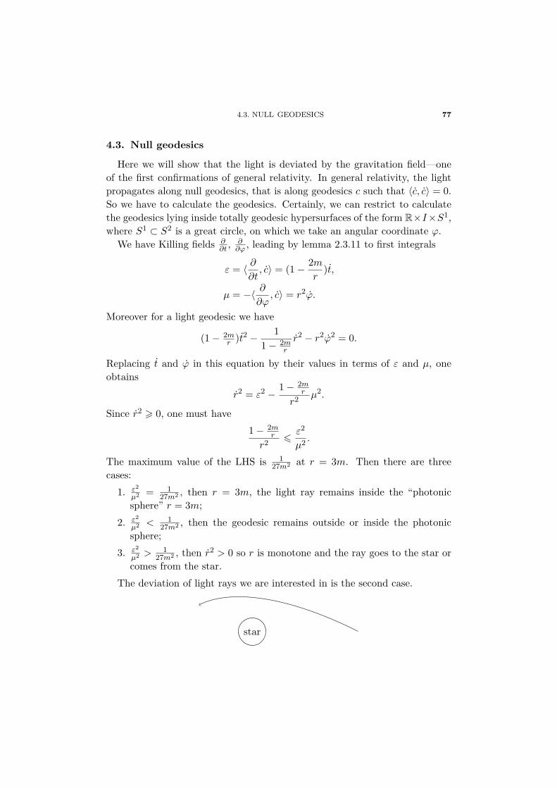
4.3. NULL GEODESICS 77

4.3. Null geodesics

Here we will show that the light is deviated by the gravitation field—oneof the first confirmations of general relativity. In general relativity, the lightpropagates along null geodesics, that is along geodesics c such that 〈c, c〉 = 0.So we have to calculate the geodesics. Certainly, we can restrict to calculatethe geodesics lying inside totally geodesic hypersurfaces of the form R×I×S1,where S1 ⊂ S2 is a great circle, on which we take an angular coordinate ϕ.

We have Killing fields ∂∂t ,

∂∂ϕ , leading by lemma 2.3.11 to first integrals

ε = 〈 ∂∂t, c〉 = (1− 2m

r)t,

µ = −〈 ∂∂ϕ

, c〉 = r2ϕ.

Moreover for a light geodesic we have

(1− 2mr )t2 − 1

1− 2mr

r2 − r2ϕ2 = 0.

Replacing t and ϕ in this equation by their values in terms of ε and µ, oneobtains

r2 = ε2 −1− 2m

r

r2 µ2.

Since r2 > 0, one must have1− 2m

r

r2 6ε2

µ2 .

The maximum value of the LHS is 127m2 at r = 3m. Then there are three

cases:1. ε2

µ2 = 127m2 , then r = 3m, the light ray remains inside the “photonic

sphere” r = 3m;2. ε2

µ2 < 127m2 , then the geodesic remains outside or inside the photonic

sphere;3. ε2

µ2 >1

27m2 , then r2 > 0 so r is monotone and the ray goes to the star orcomes from the star.

The deviation of light rays we are interested in is the second case.

star


We define ϕc = ϕ(+∞)− ϕ(−∞). For a straight line, ϕc = π. We want toprove that there is a deviation, that is ϕc > π. One has dr

dϕ = rϕ = rr2

µ , and

( drdϕ

)2 = r4

µ2(ε2 −

1− 2mr

r2 µ2)= m2

v2µ2(ε2m

2

v2 − (1− 2v)µ2) with v = m

r.

It follows that ( dvdϕ

)2 = m2ε2

µ2 − v2 + 2v3.

The variable v goes from 0 to a maximum value at, say, v0, such that v0−2v30 =

m2ε2

µ2 , and then decreases back to 0; we can rewrite( dvdϕ

)2 = v20 − 2v3

0 − v2 + 2v3,

and

ϕc = 2∫ v0

0

dϕ

dvdv = 2

∫ v0

0

dv√v2

0 − v2√

1− 2v30−v3

v20−v2

> 2∫ v0

0

dv√v2

0 − v2

(1 + v3

0 − v3

v20 − v2

)= π + 4v0.

This indeed proves that ϕc > π, so there is a deviation.For other applications of the Schwarzschild metric to general relativity, see

for example the book [Bes87].

CHAPTER 5

SOME EXERCISES

Gauss map

Let Σ be a connected compact surface embedded in R3, with sectional cur-vature K > 0. We do not suppose Σ orientable.

1 Prove that the second fundamental form of Σ is definite positive or definitenegative at every point.

2 For every x ∈ Σ we denote π the orthogonal projection R3 → (TxΣ)⊥.Prove that the vector νx = − π(∇XX)

|π(∇XX)| does not depend on the non zero vectorX ∈ TxΣ. Prove that Σ is orientable.

3 The application Γ : Σ→ S2, given by Γ(x) = νx ∈ R3, is called the Gaussmap. Prove that Γ is a diffeomorphism. Calculate Γ in case Σ = S2.

4 Prove that Γ∗ volS2 = K volΣ (how general is this formula ?) Deduce inthat case a proof of the Gauss-Bonnet formula,

12π

∫ΣK volΣ = 2.

Umbilic submanifolds

1 Let Nn−1 be a submanifold of (Mn, g), oriented by the normal ~n, withsecond fundamental form I. Prove that, for all vectors X, Y and Z of N onehas

(5.1) 〈RMX,Y Z,~n〉 = ∇XI(Y, Z)−∇Y I(X,Z).

(The RHS is (d∇I)(X,Y, Z) if one considers I as a TN -valued 1-form on N ,and this formula is the Gauss-Codazzi equation, see also remark 4.2.3.)

2 The submanifold N is said totally umbilic if for every x ∈ N the secondfundamental form is a multiple of the metric: I = λ(x)g. If N is a totally

80 CHAPTER 5. SOME EXERCISES

umbilic submanifold of the flat Rn, show that λ is a constant function. Deducethat the application φ : N → Sn−1 given by φ(x) = ~nx

λ is an isometry, andthat N is a sphere (or an open set of a sphere).

3 Find all submanifolds N ⊂ Rn with constant positive sectional curvature.

Submanifolds of the hyperbolic space

We choose coordinates in R1,n such that the quadratic form is

h(x, x) = 2x0x1 − (x2)2 − · · · − (xn)2.

The hyperbolic space is the submanifold Hn = h(x, x) = 1, x0 > 0 with theinduced metric g = −h.

1 Choose on Hn coordinates (y1, . . . , yn) ∈ R∗+ × Rn−1 by taking (x1 =1/y1, x2 = y2/y1, . . . , xn = yn/y1). Prove that

g = (dy1)2 + (dy2)2 + · · ·+ (dyn)2

(y1)2

(half-space model).2 Prove that for λ > 0 the homothety

(y1, . . . , yn)→ (λy1, . . . , λyn)

and the inversion

(y1, . . . , yn)→ (y1, . . . , yn)(y1)2 + · · ·+ (yn)2

are isometries of Hn.Prove that the intersection with Hn = y1 > 0 of a sphere of Rn centered

on the hyperplace y1 = 0 is totally geodesic.3 If g2 and g1 are Riemannian metrics on a manifold Mn such that g2 =

e2fg1, where f is a function, prove that their Levi-Civita connections satisfy

g1(∇g2XY,Z) = g1(∇g1

XY,Z) +df(X)g1(Y, Z) +df(Y )g1(X,Z)−g1(X,Y )df(Z).

Using the previous exercise, deduce that a submanifold Nn−1 ⊂ M is totallyumbilic for g1 if and only if it is totally umbilic for g2. Deduce all totallyumbilic submanifolds of Hn in the half-space model.

TORAL BLACK HOLE EINSTEIN METRICS 81

Toral black hole Einstein metrics

Let M = I × S1 × Tn−2 the product of an interval I of R, a circle S1 anda (n− 2)-dimensional torus Tn−2.

1 Find all metrics g on M , satisfying the Einstein equation

Ric(g) = −(n− 1)g,

of the form g = φ(r)dr2 + ψ(r)dθ2 + r2gT , where r and θ are coordinates onI and S1, gT is a flat metric on the torus T , and φ and ψ are functions of ronly.

Indication: first, look for a metric of the form dρ2 + F 2(ρ)dθ2 +G2(ρ)gT .2 These metrics are defined for an interval of the form I = (r+,+∞).

Which metric do we get when r+ = 0 ? prove that it is complete, withconstant sectional curvature equal to −1 (real hyperbolic cusp).

3 Prove that in some cases, one can add in r = r+ a torus Tn−2, so thatthe metric extends to a complete smooth Einstein metric on M = M ∪ Tn−2.

BIBLIOGRAPHY

[Bes87] A. L. Besse – Einstein manifolds, Springer-Verlag, Berlin, 1987.

[BGV04] N. Berline, E. Getzler & M. Vergne – Heat kernels and Diracoperators, Grundlehren Text Editions, Springer-Verlag, Berlin, 2004,Corrected reprint of the 1992 original.

[GHL04] S. Gallot, D. Hulin & J. Lafontaine – Riemannian geometry,third ed., Universitext, Springer-Verlag, Berlin, 2004.

[Kob95] S. Kobayashi – Transformation groups in differential geometry,Classics in Mathematics, Springer-Verlag, Berlin, 1995, Reprint ofthe 1972 edition.

introduction to differential geometry - …biquard/idg2008.pdf · introduction...

Documents