olivier biquard - webusers.imj-prg.fr
TRANSCRIPT

Di�erential and Riemannian Geometry
Olivier Biquard

2
Sorbonne Université, Institut de Mathématiques de Jussieu-Paris Rive Gauche
21st October 2020

Contents
I Submanifolds, manifolds 91 Submanifolds of ℝN . . . . . . . . . . . . . . . . . . . . . . . . . . . . 9
1.a Submanifold charts . . . . . . . . . . . . . . . . . . . . . . . . 91.b Tangent vectors . . . . . . . . . . . . . . . . . . . . . . . . . . 101.c Submersions . . . . . . . . . . . . . . . . . . . . . . . . . . . . 101.d Immersions . . . . . . . . . . . . . . . . . . . . . . . . . . . . 11
2 Manifolds . . . . . . . . . . . . . . . . . . . . . . . . . . . . . . . . . . 122.a Atlas and manifold . . . . . . . . . . . . . . . . . . . . . . . . 122.b The sphere . . . . . . . . . . . . . . . . . . . . . . . . . . . . 132.c The projective space . . . . . . . . . . . . . . . . . . . . . . . 142.d Submanifolds . . . . . . . . . . . . . . . . . . . . . . . . . . . 152.e Smooth maps . . . . . . . . . . . . . . . . . . . . . . . . . . . 152.f Submersions and immersions . . . . . . . . . . . . . . . . . . 16
3 Tangent vectors . . . . . . . . . . . . . . . . . . . . . . . . . . . . . . 163.a Paths and tangent vectors . . . . . . . . . . . . . . . . . . . . 163.b The tangent bundle . . . . . . . . . . . . . . . . . . . . . . . . 173.c Vector bundles . . . . . . . . . . . . . . . . . . . . . . . . . . 183.d The cotangent bundle . . . . . . . . . . . . . . . . . . . . . . 19
4 Vector �elds and bracket . . . . . . . . . . . . . . . . . . . . . . . . . 204.a Vector �elds and derivations . . . . . . . . . . . . . . . . . . . 204.b First order ordinary di�erential equations . . . . . . . . . . . 224.c Geometric interpretation of the bracket . . . . . . . . . . . . 23
5 Frobenius theorem . . . . . . . . . . . . . . . . . . . . . . . . . . . . . 246 Di�erential forms . . . . . . . . . . . . . . . . . . . . . . . . . . . . . 27
6.a Linear algebra . . . . . . . . . . . . . . . . . . . . . . . . . . . 276.b Di�erential forms on a manifold . . . . . . . . . . . . . . . . 276.c Exterior di�erential . . . . . . . . . . . . . . . . . . . . . . . . 286.d De Rham cohomology . . . . . . . . . . . . . . . . . . . . . . 306.e Orientation . . . . . . . . . . . . . . . . . . . . . . . . . . . . 306.f Integration of forms . . . . . . . . . . . . . . . . . . . . . . . 32
3

4 CONTENTS
II Riemannian metric, connection, geodesics 35
7 Riemannian metrics . . . . . . . . . . . . . . . . . . . . . . . . . . . . 357.a De�nition and examples . . . . . . . . . . . . . . . . . . . . . 357.b Volume form . . . . . . . . . . . . . . . . . . . . . . . . . . . 367.c Isometries . . . . . . . . . . . . . . . . . . . . . . . . . . . . . 37
8 Connections . . . . . . . . . . . . . . . . . . . . . . . . . . . . . . . . 378.a Connections and Christo�el symbols . . . . . . . . . . . . . . 378.b Examples of connections . . . . . . . . . . . . . . . . . . . . . 398.c Metric connections . . . . . . . . . . . . . . . . . . . . . . . . 408.d Parallel transport . . . . . . . . . . . . . . . . . . . . . . . . . 41
9 Riemannian connection, geodesics . . . . . . . . . . . . . . . . . . . . 429.a The Levi-Civita connection . . . . . . . . . . . . . . . . . . . 429.b Geodesics . . . . . . . . . . . . . . . . . . . . . . . . . . . . . 439.c Killing �elds . . . . . . . . . . . . . . . . . . . . . . . . . . . . 45
10 Exponential map . . . . . . . . . . . . . . . . . . . . . . . . . . . . . . 4610.a Exponential map and injectivity radius . . . . . . . . . . . . . 4610.b Normal coordinates . . . . . . . . . . . . . . . . . . . . . . . . 4710.c Hopf-Rinow theorem . . . . . . . . . . . . . . . . . . . . . . . 48
III Curvature 51
11 Curvature and integrability . . . . . . . . . . . . . . . . . . . . . . . . 5111.a Horizontal distribution . . . . . . . . . . . . . . . . . . . . . . 5111.b Integrability and curvature . . . . . . . . . . . . . . . . . . . 5211.c Second derivatives and curvature . . . . . . . . . . . . . . . . 54
12 Riemannian curvature . . . . . . . . . . . . . . . . . . . . . . . . . . . 5412.a Symmetries of the Riemannian curvature . . . . . . . . . . . 5412.b Sectional curvature . . . . . . . . . . . . . . . . . . . . . . . . 55
13 Second fundamental form . . . . . . . . . . . . . . . . . . . . . . . . . 5613.a Covariant derivative and second fundamental form . . . . . . 5613.b Curvature and second fundamental form . . . . . . . . . . . . 5613.c Surfaces in ℝ
3 . . . . . . . . . . . . . . . . . . . . . . . . . . . 5913.d A geometric interpretation of the curvature . . . . . . . . . . 59
14 Constant curvature metrics . . . . . . . . . . . . . . . . . . . . . . . . 6015 Riemannian curvature and topology . . . . . . . . . . . . . . . . . . . 61
15.a The conjugacy radius . . . . . . . . . . . . . . . . . . . . . . . 6115.b The Cartan-Hadamard theorem . . . . . . . . . . . . . . . . . 6115.c The Bonnet-Myers theorem . . . . . . . . . . . . . . . . . . . 62
16 Chern-Weil construction . . . . . . . . . . . . . . . . . . . . . . . . . 6416.a Extension of a connection . . . . . . . . . . . . . . . . . . . . 64

CONTENTS 5
16.b Chern-Weil homomorphism . . . . . . . . . . . . . . . . . . . 6516.c Chern classes . . . . . . . . . . . . . . . . . . . . . . . . . . . 6716.d Euler form . . . . . . . . . . . . . . . . . . . . . . . . . . . . . 67
IV Einstein equation 69
17 Ricci tensor . . . . . . . . . . . . . . . . . . . . . . . . . . . . . . . . . 6917.a Ricci and scalar curvature . . . . . . . . . . . . . . . . . . . . 6917.b The Bianchi identity . . . . . . . . . . . . . . . . . . . . . . . 7017.c Einstein equation . . . . . . . . . . . . . . . . . . . . . . . . . 70
18 Schwarzschild metric . . . . . . . . . . . . . . . . . . . . . . . . . . . 7118.a Totally geodesic submanifolds . . . . . . . . . . . . . . . . . . 7118.b The equations and the Schwarzschild metric . . . . . . . . . . 7218.c Null geodesics . . . . . . . . . . . . . . . . . . . . . . . . . . . 74
V Some exercises 77
Bibliography 80
Index 82

6 CONTENTS

Introduction
These are notes for an introductory course in di�erential geometry. The aim is togive some basis on several topics: manifolds, vector �elds, connections, curvature,Riemannian geometry, Einstein equation. As an illustration we �nish by the calcu-lation of the Schwarzschild metric—the simplest model in general relativity for thegravitational �eld of a star like our sun or our earth—, and as �rst application, weexplain the deviation of light rays by the sun.The notes are not intended as a self-contained reference: sometimes the proofs areomitted, short or left to the reader as exercises. The reader should complete thesenotes by referring to an excellent textbook like [GHL04]. On Einstein metrics at theend of the notes, a standard reference is [Bes87]. A few exercises are proposed in thetext, some other ones at the end of the notes.
7

8 CONTENTS

Chapter I
Submanifolds, manifolds
This chapter is a concise introduction to smooth manifolds, an excellent referencewith all the required details is [Lee13].
1 Submanifolds of ℝN
1.a Submanifold charts
A submanifold of ℝN of dimension n is a subset of ℝN which is locally di�eomorphicto ℝ
n× {0} ⊂ ℝ
N. More formally:
De�nition 1.1. A submanifold of ℝN of dimension n is a subset M ⊂ ℝN such that,
for each x ∈ M, there exists an open neighborhood U of x in ℝN, an open set V ⊂ ℝ
N,and a di�eomorphism ϕ ∶ U→ V such that
ϕ(U ∩ M) = V ∩ (ℝn× {0}).
We call such a map ϕ a chart of M.
Very often, we shall abbreviate ‘a n-dimensional submanifold M of ℝN’ in ‘a subman-ifold Mn of ℝN’.One simple example is the 2-sphere
S2= {x
2+ y
2+ z
2= 1}
which is a 2-dimensional submanifold of ℝ3. Indeed, consider the open set U = {z >
0, x2+ y
2< 1} of ℝ3, then the map ϕ ∶ U→ ℝ
3 de�ned by
ϕ(x, y, z) = (x, y, z −
√
1 − x2− y
2)
is a di�eomorphism onto an open set of ℝ3, and takes the sphere into ℝ2× {0}. By
permuting the variables ±x , ±y and ±z, one can cover the sphere with similar opensets and charts.Similarly, the n-dimensional sphere
Sn= {(x
0)2+⋯ + (x
n)2= 1}
is a submanifold of ℝn+1.
9

10 CHAPTER I. SUBMANIFOLDS, MANIFOLDS
Exercise. If f ∶ U ⊂ ℝn→ ℝ
N−n is a smooth map de�ned on an open set U in ℝn ,
then the graph M = {(x, f (x)), x ∈ U} is a n-dimensional submanifold of ℝN.For example, the n-dimensional hyperbolic space
Hn= {(x
0,… , x
n) ∈ ℝ
n+1, x0> 0, (x
0)2− (x
1)2−⋯ (x
n)2= 1} (I.1)
is a submanifold of ℝn+1.
1.b Tangent vectors
We now de�ne what it means for a vector of ℝN to be tangent at x to a submanifoldpassing through x .
De�nition 1.2. If M is a submanifold of ℝN and x ∈ M, then a vector X ∈ ℝN is a
tangent vector to M at x if there exists a C1 curve c ∶] − ϵ, ϵ[→ M ⊂ ℝN, such that
c(0) = x and c′(0) = X.
The space of all tangent vectors to M at x is called the tangent space of M at x andis noted TxM.
Example 1.3. 1° If Mn is an a�ne subspace of ℝN, so M = x0 + V where V is a vectorsubspace of ℝN, then for all x ∈ M, one has TxM = V.2° Suppose f ∶ U ⊂ ℝ
N→ V ⊂ ℝ
N is a di�eomorphism between two open sets Uand V. If c(t) ∈ M ∩ U with c(0) = x , then f (c(t)) ∈ f (M) ∩ V and d
dtf (c(t))|t=0 =
dx f (c′(0)). It follows that X ∈ TxM if and only if dx f (X) ∈ Tf (x)(f (M)). So we obtain
an isomorphism
TxM
dx f
⟶ Tf (x)
(f (M)).
Let us now use these two examples together: near a point x ∈ M take a chart ϕ ∶ U ∋x → V ⊂ ℝ
N, with ϕ(M ∩ U) = (ℝn× {0}) ∩ V, then it follows that
TxM = (dxϕ)−1(ℝ
n× {0}).
This proves that TxM is always a n-dimensional vector subspace of ℝN.
1.c Submersions
Recall that a map from an open set of ℝN to ℝN−n is called a submersion if its di�er-
ential is surjective at any point.
Theorem 1.4. If a map f ∶ U ⊂ ℝN→ ℝ
N−n is a submersion, then for any b ∈ ℝN−n ,
the set f −1(b) (if non empty) is a n-dimensional submanifold of ℝN, and its tangent spaceat a point x ∈ f
−1(b) is
Tx f−1(b) = ker(dx f ).
Proof. Let x ∈ f−1(b). Choose a supplementary subspace F ≃ ℝ
N−n of ker(dx f ) in ℝN,
such that ℝN = ker(dx f ) ⊕ F. Then the map dx f ∶ F → ℝN−n is an isomorphism.
Consider the map ϕ ∶ U→ ℝn× ℝ
N−n:
ϕ(x + (u, v)) = (u, f (x + (u, v)) − b), u ⊕ v ∈ ker(dx f ) ⊕ F = ℝN.

1. SUBMANIFOLDS OF ℝN 11
Its di�erential,dxϕ(u, v) = (u, dx f (v)),
is an isomorphism, so by the inverse function theorem, the map ϕ is a di�eomorphismon a small neighborhood V of x . Clearly, f −1(b) ∩ V = ϕ−1(ℝn
× {0} ∩ ϕ(V)), so ϕ is achart for f −1(b) near x , and
Tx (f−1(b)) = (dxϕ)
−1(ℝ
n× {0}) = ker(dx f ).
Remark 1.5. Since ϕ is a local di�eomorphism, one can write near x the map f asf = g◦ϕ + b, where g ∶ ℝ
N→ ℝ
N−n is given by
g(x1,… , x
N) = (x
n+1,… , x
N). (I.2)
So the meaning of the theorem is that, up to a di�eomorphism, any submersion hasthe local form (I.2).Example 1.6. 1° The curve y
2= x
3− x is a smooth curve (that is a 1-dimensional
submanifold of ℝ2. Indeed, consider f (x, y) = y2− x
3+ x , then d
(x,y)f = (−3x
2+ 1, 2y)
which vanishes only at the points (± 1√
3, 0). Since these two points are not in f
−1(0),
the result follows from the theorem applied to the map f on the open set U = ℝ2⧵
{(±1√
3, 0)}.
2° The sphere Sn = {(x0)2+ ⋯ + (x
n)2= 1} and the hyperbolic space Hn
= {x0>
0, (x0)2− (x
1)2−⋯ (x
n)2= 1} are submanifolds of ℝn+1.
3° (Exercise) The group O(n) is a submanifold of ℝn2 (the space of n × n matrices).
Apply the theorem to the map f (A) = AAt− 1 from matrices to symmetric matrices.
To prove that f is a submersion at each point x ∈ O(n), use the invariance f (Ax) = f (A)
to reduce to the case x = 1.
1.d Immersions
We now pass to immersions: recall that a map f from an open set U ⊂ ℝn to ℝ
N iscalled an immersion if dx f is injective at each x ∈ U.Example 1.7. 1° The map ℝ
n→ ℝ
n+1 given by (x1,… , x
n) ↦ (1 + (x
1)2+ ⋯ +
(xn)2, x1,… , x
n) is an immersion and a bijection from ℝ
n to its image Hn⊂ ℝ
n+1,the hyperbolic space.2° The two �gures below represent immersions ℝ → ℝ
2 whose image is not a sub-manifold: the �rst is not injective, it has a double point; the second one is injectivebut not proper.

12 CHAPTER I. SUBMANIFOLDS, MANIFOLDS
De�nition 1.8. We say that a map f ∶ U ⊂ ℝn→ ℝ
N is an embedding, if f is animmersion and f is an homeomorphism from U to f (U).
Lemma 1.9. 1° A proper injective immersion is an embedding.2° If f ∶ U ⊂ ℝ
n→ ℝ
N is an embedding, then f (U) is a n-dimensional submanifold ofℝN.
Proof. See for example the book [Lee13].
2 Manifolds
2.a Atlas and manifold
De�nition 2.1. Let M be a topological space. A C∞ atlas on M is the data of
1. an open covering (Ui)i∈I of M,
2. homeomorphisms ϕi ∶ Ui → Vi ⊂ ℝn onto open sets of ℝn ,
such that for any i and j, the composite
ϕi◦ϕ−1
j∶ ϕj (Ui ∩ Uj )→ ϕi(Ui ∩ Uj )
is a C∞ di�eomorphism.
The maps ϕi◦ϕ−1j are called the transition functions of the atlas.
Example 2.2. If Mn is a submanifold of ℝN, then for any point x ∈ M, we have a chartϕx ∶ U ⊂ ℝ
N→ ℝ
n× ℝ
N−n sending U ∩ M to ℝn× {0}. Denote by π the projection
ℝn× ℝ
N−n→ ℝ
n , then the collection (π◦ϕx )x∈M is an atlas for M.
Two atlas are equivalent atlases if their union is an atlas. Concretely this means thatif ϕi and ψj are the charts of the �rst and second atlas, then the compositions ϕi◦ψ−1jare C∞ on the open sets where they are de�ned.
De�nition 2.3. A manifold M is the data of:
1. a topological space M which is Hausdor� and countable at in�nity (that is acountable union of compact sets);
2. an equivalence class of C∞ atlas on M.
The integer n appearing in the de�nition of an atlas is the dimension of M. It isconstant on each connected component of M. (One usually considers manifolds withall the connected components sharing the same dimension).Example 2.2 shows that a submanifold ofℝN is a manifold, there is only the topologicalassumption of being countable at in�nity to prove (exercise): prove that a submanifoldM ⊂ ℝ
N is locally closed, that is the intersection of a closed set (M) and of an open setof ℝN (the union of the images of the submanifold charts); prove that an open set ofℝN is countable at in�nity, and conclude.

2. MANIFOLDS 13
Remark 2.4. One can de�ne also the notion of a Ck atlas and a Ck manifold by askingthat the transition functions ϕi◦ϕ−1j be only in C
k . The fact that the dimension islocally constant remains obvious for k > 0, but is a more di�cult topological resultfor k = 0 (in that case, one says that M is a topological manifold).Remark 2.5. If the dimension is even, n = 2m, then the charts take values in ℂ
m=
ℝ2m . If the transition functions ϕiϕ−1j are holomorphic maps, then the manifold is a
complex manifold.Remark 2.6. One can de�ne an abstract atlas on a set M in the same way we de�nedan atlas, but we drop the assumption that the transitions are homeomorphisms, sincewe have no topology. Actually an abstract atlas on M induces a unique topology onM: it is de�ned by saying that U ⊂ M is open if the image ϕi(U ∩ Ui) by each chart ϕiis an open set of ℝn . The uniqueness implies that the topology de�ned by an atlas ona topological space M coincides with the given topology of M.The topological assumptions onM in the de�nition 2.3 can be checked directly on theatlas:
• M is Hausdor� if for each charts ϕi , ϕj the set {(x,ϕi◦ϕ−1j (x), x ∈ ϕj (Ui ∩ Uj )}
(the graph of the transition) is closed in ϕj (Uj ) × ϕi(Ui);
• M is countable at in�nity if the atlas contains a countable sub-atlas.
Therefore we can de�ne a manifold structure on a set M just by giving an abstractatlas, and checking the two above conditions to get a good topology on M.
2.b The sphere
It is a good point to stop after this rather abstract de�nition, and to consider what itmeans on the concrete example of the sphere Sn . In coordinates (x0,… , x
n), the north
poleN and the south pole S are the points (±1, 0,… , 0). We now de�ne two charts withvalues in ℝ
n , considered as the hyperplane {x0 = 0} in ℝn+1. For x ∈ Sn ⧵ {N} de�ne
the stereographic projection ϕN(x) from the north pole to be the point of ℝn wherethe line passing through N and x meets ℝn; the stereographic projection ϕS from thesouth pole is de�ned similarly:
N
x
ϕN(x) ϕS(x)
S
x
In formulas:
ϕN(x0, x1,… , x
n) =
(x1,… , x
n)
1 − x0
, ϕS(x0, x1,… , x
n) =
(x1,… , x
n)
1 + x0
.

14 CHAPTER I. SUBMANIFOLDS, MANIFOLDS
The transition function is the inversion
ϕNϕ−1
S(x1,… , x
n) =
(x1,… , x
n)
(x1)2+⋯ + (x
n)2.
This is now an ‘abstract’ description of the sphere, meaning that it does not rely onseeing it as a submanifold of ℝn+1.
2.c The projective space
Our next example will be de�ned directly as an abstract manifold. It is the real pro-jective space ℝP
n of all real lines in ℝn+1. This can be identi�ed with the quotient
Sn/(ℤ/2) of the sphere by the antipodal map.
A nonzero vector (x0,… , xn) ∈ ℝ
n generates a line in ℝn , that is a point of ℝPn which
is denoted [x0 ∶ ⋯ ∶ xn]. Therefore, if λ is any non vanishing number, one has
[x0∶ ⋯ ∶ x
n] = [λx
0∶ ⋯ ∶ λx
n].
The [x0 ∶ ⋯ ∶ xn] are the homogeneous coordinates on ℝP
n . We turn ℝPn into a
manifold by giving an explicit atlas, and by checking that the transition functions aresmooth: let Ui ⊂ ℝP
n the open set given by Ui = {xi ≠ 0}. On Ui we have the chartϕi ∶ Ui → ℝ
n given by
ϕi([x0∶ ⋯ ∶ x
n]) = (
x0
xi,… ,
xi
xi,… ,
xn
xi),
where the hat means that this term is omitted. The transition function ϕiϕ−1j ∶ ϕj (Ui ∩
Uj )→ ϕi(Ui ∩ Uj ) is given by
ϕiϕ−1
j(x1,… , x
n) = (
x1
xi,… ,
xj−1
xi,
1
xi,
xj+1
xj,… ,
xi
xi,… ,
xn
xj).
The reader can check that the topological conditions listed in remark 2.6 are satis�ed.The ℝP
n for di�erent n’s are related in the following way. The chart open set Un =
{xn= 1} is di�eomorphic to ℝ
n by ϕn . The complement
ℝPn⧵ Un = {[x
0∶ ⋯ ∶ x
n−1∶ 0]}
identi�es naturally with ℝPn−1. In this way one obtains the ℝPn inductively: starting
from ℝP0 which is reduced to a point,
• ℝP1= ℝ ∪ {pt.} is a circle;
• ℝP2= ℝ
2∪ ℝP
1 is the union of the plane and the line at in�nity;
• more generally, ℝPn = ℝn∪ ℝP
n−1.
Finally, observe that all we have done has a meaning if we decide that the x i are com-plex coordinates rather than real coordinates. In this way, one obtains the structure ofa complex manifold on the complex projective space ℂP
m of complex lines in ℂm+1.
In particular, one obtains thatℂP
1= ℂ ∪ {pt.}
which will turn to be di�eomorphic to a 2-sphere.

2. MANIFOLDS 15
2.d Submanifolds
The notion of submanifold of ℝN studied in section 1 extends to a notion of subman-ifold of a manifold. Quick de�nition: Xn
⊂ MN is a submanifold if for each chart ϕ
de�ned on an open set U ⊂ M, then ϕ(X ∩ U) is a submanifold of ϕ(U) ⊂ ℝN. This
means that up to a di�eomorphism of ℝN, one has ϕ(X ∩ U) = ϕ(U) ∩ (ℝn× {0}). So a
more formal de�nition is:
De�nition 2.7. A set Xn⊂ M
N is a submanifold of MN if near each point of M, thereis a chart ϕ ∶ U ⊂ M→ V ⊂ ℝ
N such that ϕ(X ∩ U) = (ℝn× {0}) ∩ V ⊂ ℝ
n× ℝ
N−n .
A submanifold X inherits a manifold structure, for which the charts are the restrictionof the submanifold charts to X. In particular the submanifolds of ℝN are manifolds.
2.e Smooth maps
A chart on a manifold Mn is a local map ϕ = (x1,… , x
n) to ℝ
n . The (x1,… , xn) are
local functions on M called local coordinates. A map f ∶ Mn→ ℝ
p is locally anapplication of n variables
f (x1,… , x
n) = (f1(x
1,… , x
n),… , fp(x
1,… , x
n)),
and we declare it to be smooth if each fi is a smooth function of the variables (x1,… , xn).
If the target is a manifold Np , we have also coordinates on Np , and we have to replacethe (fi) by local coordinates on N as well. This leads to the following de�nition.
De�nition 2.8. A smooth map between two manifolds Mn and Np (or C∞ map) isa continuous map f ∶ M
n→ N
p such that for any charts ϕ ∶ U ⊂ M → ℝn and
ψ ∶ V ⊂ N→ ℝp , the map
ψfϕ−1∶ ϕ(U ∩ f
−1(V)) ⊂ ℝ
n→ ψ(V) ⊂ ℝ
p
is C∞.
As we have just seen, this de�nition means that in the charts, the coordinates of f (x)are smooth functions of the coordinates of x . Of course the de�nition does not dependon the choice of charts, because the transition between two charts is always a C∞di�eomorphism.If f ∶ Mn
→ Np is smooth and a bijection such that f −1 is also smooth, we say that
f is a C∞ di�eomorphism. Of course this implies n = p. In that case we say that Mand N are di�eomorphic.Example 2.9. 1° A map f ∶]a, b[→ M
n is smooth if for any chart ϕ ∶ U ⊂ M→ ℝn the
composite ϕ◦f is smooth. Write ϕ = (x1,… , xn) (the (x i) are called local coordinates
on M), the map f can be locally written f = (f1,… , f
n) where f
i= x
i◦f . Then f is
smooth means that each fi is C∞ as a real function of one real variable.
2° A function f ∶ Mn→ ℝ is smooth if for any chart ϕ = (x
1,… , x
n) as above, the
function f ◦ϕ−1 on ℝ
n is smooth, that is f is smooth as a function of (x1,… , xn). One
often identi�es U with its image in ℝn and then one can write directly f (x
1,… , x
n).
Exercise. 1° Prove that the following maps are smooth:

16 CHAPTER I. SUBMANIFOLDS, MANIFOLDS
• the quotient by the antipodal map Sn → ℝPn;
• the map S3 → ℂP1 taking a vector x ∈ S3 to the complex line that it generates
in ℂ2.
2° Prove that S2 and ℂP1 are di�eomorphic.
2.f Submersions and immersions
From the de�nition, a smooth map f ∶ Mn→ N
p between two manifolds is just loc-ally a smooth map from ℝ
n to ℝp . It is easy to see that the notions of submersion and
immersion do not depend on the choice of the charts, so it makes sense to speak aboutf being a submersion or an immersion. Then the results of section 1 on submanifoldsof ℝN extend to abstract manifolds, in particular we have the notion of embedding ofa manifold into another manifold from de�nition 1.8, and theorem 1.4 and lemma 1.9can be applied in this more general setting.Remark 2.10. Any manifold M
n can be embedded in ℝN for N large enough, so is
di�eomorphic to a submanifold of ℝN. A theorem of Whitney gives a bound on N interms of n: the ‘easy’ version is N = 2n + 1 (see [Lee13]), but Whitney actually provedthat it is possible to take N = 2n.
3 Tangent vectors
3.a Paths and tangent vectors
We now turn to the notion of a tangent vector at a point x in a manifold M. Recallthe case of submanifolds of ℝN (de�nition 1.2): a tangent vector at x to a submanifoldM ⊂ ℝ
N is the derivative c′(0) of a path c ∶] − ϵ, ϵ[→ M such that c(0) = x . Of course
two paths c1 and c2 de�ne the same tangent vector if c′1(0) = c
′
2(0). It turns out that
this point of view leads to a good de�nition for an abstract manifold:
De�nition 3.1. Let M be a manifold and x a point of M.1°We say that two paths c1, c2 ∶]−ϵ, ϵ[→ M such that c1(0) = c2(0) = x are equivalentpaths if for any local chart ϕ at x , one has
(ϕ◦c1)′(0) = (ϕ◦c2)
′(0).
2° A tangent vector at x to M is an equivalence class of paths for this relation.3° The set of all tangent vectors at x to M is called the tangent space of M at x andnoted TxM.
Observe that in the �rst part of the de�nition, it is equivalent to ask the equality ofthe derivatives for one chart or for all charts.If we have a smooth map between two manifolds, f ∶ Mn
→ Np , then to a path c at
x ∈ M we can associate the path f (c) at f (x). It is easy to check that if c1 and c2 areequivalent, then so are f (c1) and f (c2). It follows that we obtain a well de�ned map
dx f ∶ TxM→ Tf (x)
N. (I.3)

3. TANGENT VECTORS 17
If f is a di�eomorphism, then it is easy to check that (dx f )−1 = dx (f−1).
Apply this to a local chart ϕ at x : the map ϕ is a di�eomorphism U ⊂ M → V ⊂ ℝn ,
so we obtain an isomorphism
dxϕ ∶ TxM⟶ℝn, c ⟼ (ϕ◦c)
′(0).
We would like to deduce that TxM is a vector space, since it is identi�ed to ℝn . Again,
this will be true if it does not depend on the chart ϕ. This is a good place to checkthis kind of statement, that we are using repeatedly: if we have another chart ψ, sowe have a transition function ψϕ−1, then the following diagram is commutative (wecan assume that the chart is centered: ϕ(x) = 0):
TxM
dxϕ ↙ ↘dxψ
ℝn
d0(ψϕ−1)
−−−−−−−−−→ ℝn
So the two di�erent identi�cations of TxM with ℝn di�er by the linear isomorphism
d0(ψϕ−1), which preserves the vector space structure. So the vector space structures
induced on TxM from dxϕ and dxψ coincide.
3.b The tangent bundle
We now turn to the problem of constructing the manifold of all tangent vectors at allpoints of a manifold M. First consider the case of a submanifold Mn
⊂ ℝN. Then we
can considerTM = {(x,X) ∈ M × ℝ
N,X ∈ TxM} ⊂ ℝ
N× ℝ
N.
Then (exercise):
1. TM is a submanifold of ℝN × ℝN: if ϕ ∶ U ⊂ ℝN→ ℝ
N is a local submanifoldchart for M, then
U × ℝN⟶ ℝ
N× ℝ
N, (x,X)↦ (ϕ(x), dxϕ(X))
is a submanifold chart for TM;
2. the projection (x,X) → x gives a map π ∶ TM → M, such that π−1(x) = TxM,that is the �bers are the tangent spaces of M.
Observe that in particular, for an open set U ⊂ ℝn , we simply have TU = U × ℝ
n: thetangent vectors to U at a point identify to ℝ
n .Now pass to an abstract manifold M: there is a way to do the same construction, butthe result TM will be a manifold instead of a submanifold of ℝN ×ℝN. Let us describeit now:
• as a set, TM = ∐x∈M
TxM = {(x,X), x ∈ M,X ∈ TxM}; there is a projectionπ ∶ TM→ M given by π(x,X) = x ;
• the manifold structure is described by the following charts: if ϕ ∶ U ⊂ M→ ℝn
is a chart for M, then a chart dϕ ∶ π−1(U) ⊂ TM→ ℝ2n for TM is given by
dϕ(x,X) = (ϕ(x), dxϕ(X)).

18 CHAPTER I. SUBMANIFOLDS, MANIFOLDS
We now write the transition functions for this atlas. In particular this will prove thatTM has indeed a manifold structure. Suppose we have two charts ϕ1 and ϕ2 of Mde�ned on open sets Ui , then we have the charts dϕi of TM de�ned on π−1(Ui). Onthe intersectionU12 = U1∩U2, the two charts are related by the following commutativediagram:
π−1(U12)
dϕ1 ↙ ↘dϕ2
ϕ1(U12) × ℝn⊂ ℝ
n× ℝ
nd(ϕ2ϕ
−1
1)
−−−−−−−−−→ ϕ2(U12) × ℝn⊂ ℝ
n× ℝ
n
(I.4)
where of course d(ϕ2ϕ−1
1) is the di�erential of the transition function ϕ2ϕ−11 , that is
d(ϕ2ϕ−1
1)(x,X) = (ϕ2ϕ
−1
1(x), dx (ϕ2ϕ
−1
1)(X)).
Therefore we have an atlas on TM, and using remark 2.6 one can check that it de�nesa Hausdor�, countable at in�nity, topology on TM. Therefore TM is a manifold ofdimension 2n.Now come back to a smooth map f ∶ M
n→ N
p , then the collection of the mapsdx f ∶ TxM → TxN gives a smooth tangent map df ∶ TM → TN preserving thevector bundle structure, that is one has the commutative diagram
TM
df
⟶ TN
↓ ↓
M
f
⟶ N
where for each x the induced map dx f ∶ TxM → Tf (x)
N is a linear map. Let usgive concrete formulas (and this will prove that df is indeed a smooth map betweenmanifolds): in local coordinates (x i) on M and (y j ) on N (recall that this means thatthe local map M→ ℝ
n given by the (x i) is a chart), we can write
f = (f1(x1,… , x
n),… , f
p(x1,… , x
n)),
and then df is calculated as
df (x1,… , x
n,X
1,… ,X
n) = (f
1,… , f
p,X
i)f
1
)xi,… ,X
i)f
p
)xi). (I.5)
In this formula we used the implicit summation convention: if we �nd in a formulathe same i as an index and as an exponent, then one must understand that the resultis just the sum on all possible i’s, so in the above formula Xi )f
j
)xi
means ∑n
i=1Xi )f
j
)xi.
So we see that df is nothing but the abstract version (for manifolds) of the di�erentialof a map ℝ
n→ ℝ
p . In particular one has the composition formula
d(g◦f ) = dg◦df .
3.c Vector bundles
The transition functions (I.4) of TM are of a special kind: for each x ∈ ϕ1(U12), therestriction of d(ϕ2ϕ−11 ) to {x} × ℝn is a linear isomorphism (actually this is a way tosee that each �ber π−1(x) has a vector space structure). This a special example of the

3. TANGENT VECTORS 19
more general notion of a vector bundle over M: a rank p vector bundle E over M is amanifold E with a smooth map π ∶ E → M, and charts of the type (I.4), called localtrivializations:
ψi ∶ π−1(Ui) ⟶ Ui × ℝ
p
π ↘ ↙
Ui
where the diagram is commutative, such that the transition functions
ψiψ−1
j∶ π
−1(Uij ) × ℝ
p⟶ π
−1(Uij ) × ℝ
p
have the form
ψiψ−1
j(x, ξ) = (x, uij (x)(ξ)), uij ∶ Uij → GLpℝ smooth.
(Note that here we have not exactly charts as in equation (I.4) because we have notapplied a local chart ϕi to the x part of (x, ξ); to have true manifold charts for E weshould compose ψi with (ϕi , 1ℝp ).)From the local trivializations of a vector bundle π ∶ E→ M and the transitions func-tions, we see immediately that the �bers Ex ∶= π−1(x) have a vector space structure.The vector bundle structure is completely characterized by the set of GLpℝ valuedtransition functions (uij ) on Uij . They satisfy uji = u
−1
ijand the cocycle identity
uijujkukj = 1 on Ui ∩ Uj ∩ Uk.
Conversely, such a set of transition functions relative to some covering (Ui) of Mde�nes a vector bundle on M, de�ned by (exercise)
E = (∐
i
Ui × ℝp)/(j, x, ξ) ∼ (i, x, uij (x)ξ) if x ∈ Uij .
Also remark that one can de�ne similarly complex rank p vector bundles, where thetransition functions take their values in the group GLpℂ of complex linear isomorph-isms.Finally, a smooth section of a vector bundle E is a C∞ map s ∶ M → E such thatπ◦s = 1M. This just means s(x) ∈ Ex for each x . In a local trivialization E|Ui ≃ Ui ×ℝ
p ,such a section is given by p coordinates s1(x),… , sp(x) which are smooth functions.The set of smooth sections (resp. compactly supported smooth sections) of E over Mwill be denoted Γ(M,E) (resp. C∞
c(M,E)). If there is no ambiguity we may abbreviate
into Γ(E) and C∞c(E).
If E is the trivial vector bundle M×ℝ, then sections of E are just smooth functions onM. The algebra of smooth functions on M is noted C∞(M).If s, t ∈ Γ(M,E) and f ∈ C
∞(M), then s + t (de�ned by (s + t)(x) = s(x) + t(x)) and f s
(de�ned by (f s)(x) = f (x)s(x)) are still smooth sections of E (exercise), that is s + t andf s ∈ Γ(M,E). Therefore Γ(M,E) is a C∞(M)-module.
3.d The cotangent bundle
An important example of vector bundle is the cotangent bundle of a manifold Mn .This is a vector bundle, denoted T∗M, whose �ber at x ∈ M is the dual T∗
xM of the

20 CHAPTER I. SUBMANIFOLDS, MANIFOLDS
tangent space TxM. If we want to de�ne T∗M by transition functions, we use a cover-ing of M by open sets (Ui) on which TM is trivialized, with transition functions (uij );then it is easy to see that the transition functions for T∗M are (tu−1
ij).
If f ∶ M → ℝ is a smooth function, its di�erential dx f is a linear form on TxM, sodx f ∈ T
∗
xM. It follows that df can be interpreted as a section of T∗M. Sections of T∗M
are called 1-forms. If (x i) are local coordinates, then a local basis of T∗M is given bythe di�erential dx i of the coordinates. Then, for any function f the formula (I.5) canbe written
df =
)f
)xidx
i,
which actually proves that df is a smooth section of T∗M.This construction of the cotangent bundle is just a special case of the following generalfact. If we have one or several bundles, any algebraic operation on the underlyingvector spaces can be done �berwise to give rise to a new vector bundle. For example,if E and F are vector bundles, then E⊕F, E⊗F andHom(E, F) are vector bundles, whose�bers at x ∈ M are Ex ⊕ Fx , Ex ⊗ Fx and Hom(Ex , Fx ). The proof is left as an exercise.
4 Vector �elds and bracket
4.a Vector �elds and derivations
If f ∶ M → ℝ is a smooth function, then at each point x ∈ M we have a di�erentialdx f ∶ TxM→ ℝ. If X ∈ TxM is a tangent vector at x , then we can consider the map
DX ∶ f ⟶ dx f (X). (I.6)
It satis�es the Leibniz rule
DX(f g) = (DXf )g(x) + f (x)(DXg).
Now suppose that we have a tangent vector X(x) ∈ TxM for each x ∈ M, dependingsmoothly on x , that is X is a section of TM (smooth sections of TM are called vector�elds). The map (I.6) considered for all x together gives a map, called Lie derivative
LX ∶ C∞(M)⟶ C
∞(M), f ⟼ df (X), (I.7)
satisfying the Leibniz rule
LX(f g) = (LXf )g + fLXg.
So the Lie derivative is a derivation of the algebra C∞(M).Let us see what this means in local coordinates (x i) on M. Then the tangent bundle islocally identi�ed with ℝ
n , and we consider the basis vector �elds
e1 = (1, 0,… , 0),… , en = (0,… , 0, 1).
Any local vector �eld X can be written as X = Xiei (recall the implicit summation
convention). If f is a function on M, we can consider locally f as a function of thelocal coordinates, f (x1,… , x
n). Then we check easily that
Leif =
)f
)xi. (I.8)

4. VECTOR FIELDS AND BRACKET 21
This is why the vector �eld ei is usually identi�ed with the corresponding derivation,ei =
)
)xi. In the sequel we will use the notation )
)xi
instead of ei .We now generalize this identi�cation. If we have a commutative ℝ-algebra A, thena derivation of A is a ℝ-linear map D ∶ A → A satisfying the Leibniz formulaD(ab) = (Da)b + a(Db). The set of all derivations of A is noted D(A).The main result in this section says that a vector �eld is the same thing as a derivationof the algebra C∞(M):
Theorem 4.1. The map X↦ LX is an isomorphism Γ(TM)→ D(C∞(M)).
Proof. Let D be a derivation of C∞(M). We want to �nd a vector �eld X such thatD = LX.First step: D is a local operator, that is if U is open, then
f |U = 0⇒ (Df )|U = 0. (I.9)
This implies that if f and g coincide on U, then D(f − g)|U = 0 so Df and Dg coin-cide on U: in particular Df (x) depends only on the values of f on an arbitrary smallneighborhood of x . Now prove (I.9): choose a function χ with compact support in U,then
D(χf ) = χDf + (Dχ)f .
If f |U = 0, then χf = 0 so χDf = −(Dχ)f vanishes on U.Note that we can now de�ne Df for f de�ned on any open set U ⊂ M. Indeed supposex ∈ V ⊂⊂ U, we can choose χ with compact support in U such that χ|V = 1, thenχf ∈ C
∞(M) and we can de�ne (Df )(x) ∶= D(χf )(x). This does not depend on the
choices.Second step: D(1) = 0. This is clear, since D(12) = 1D(1) + D(1)1 = 2D(1).Third step: local. Take local coordinates (x i) and write
f (x1,… , x
n) = f (0) + x
igi(x
1,… , x
n)
for smooth functions gi . Because of the �rst step, we can apply D to these local func-tions: using Leibniz identity we get
(Df )(0,… , 0) =
n
∑
1
(Dxi)(0,… , 0)gi(0,… , 0)
=
n
∑
1
(Dxi)(0,… , 0)
)f
)xi(0,… , 0)
So we must haveX(0) = (Dx i)(0,… , 0))
)xi. Doing this at each point x of the chart gives
X(x) = (Dxi)(x)
)
)xi. (I.10)
This proves the uniqueness of X, and the local existence of X.For the existence, we de�ne X on each coordinate open set by (I.10), then by theuniqueness statement the various vector �elds de�ned on the open sets must coincideon the intersections, so they glue together to de�ne the expected vector �eld.

22 CHAPTER I. SUBMANIFOLDS, MANIFOLDS
The theorem enables to de�ne easily the bracket of two vector �elds:
De�nition 4.2. If X and Y are two vector �elds on M, then their bracket [X,Y] is thevector �eld corresponding to the derivation [LX,LY] = LXLY −LYLX.
This rather abstract de�nition corresponds to a simple calculation: taking local co-ordinates (x i), we write X = Xi )
)xi
and Y = Yi )
)xi, then
LXLYf −LYLXf = Xj)
)xj(Y
i)f
)xi) − Y
j)
)xj(X
i)f
)xi)
= (Xj)Y
i
)xj− Y
j)X
i
)xj)
)f
)xi
Therefore[X,Y] = (X
j)Y
i
)xj− Y
j)X
i
)xj)
)
)xi. (I.11)
Lemma 4.3. 1° [X, fY] = f [X,Y] + (LXf )Y.
2° Jacobi identity: [X, [Y,Z]] + [Y, [Z,X]] + [Z, [X,Y]] = 0.
3° If N is a submanifold ofM and the restrictions of X and Y to N lie inside TN ⊂ TM|N,then [X,Y]|N is tangent to N and equals [X|N,Y|N].
Proof. The proof is easy given the explicit formula (I.11) for the bracket, and is left tothe reader. The Jacobi identity is best seen as the consequence of the obvious corres-ponding algebraic identity
[LX, [LY,LZ]] +⋯ = 0.
4.b First order ordinary di�erential equations
If we have a smooth curve c ∶ I → M in M, de�ned on an interval I ⊂ ℝ, then foreach t we can consider the derivative c(t) = dtc(
)
)t) ∈ T
c(t)M. Let X be a vector �eld
on the manifold Mn , we look for solutions c ∶ I→ M of the equation
c = X(c). (I.12)
Note that for each t ∈ I, both c(t) and X(c(t)) belong to Tc(t)M, so the equation makes
sense.For example, if M = ℝ
2, then a vector �eld is X = f (x, y))
)x+ g(x, y)
)
)y, the curve is
c(t) = (x(t), y(t)) and the equation (I.12) is the system{
x = f (x, y)
y = g(x, y).
More generally, in local coordinates (x i), the equation (I.12) becomes
xi= X
i(x1,… , x
n).

4. VECTOR FIELDS AND BRACKET 23
So if we give the initial condition c(t0) ∈ M, near t0 the path c(t) will remain in theopen set of coordinates and the equation (I.12) translates into a �rst order system ofordinary di�erential equations. Usual results then say that the equation has a uniquesolution in a small interval containing t0.It follows that if we give the initial condition c(0) = x ∈ M, there is a unique solutionde�ned on a maximal interval I ∋ x . We shall denote this solution cx (t).
De�nition 4.4. The vector �eld X on M is a complete vector �eld if for any initialcondition x , the solution cx is de�ned on ℝ.
Lemma 4.5. If a vector �eld X has compact support, then X is complete.
Proof. The only way a solution can exist only on a bounded interval is that c(t) getsout of any compact of M. But this is impossible since X = 0 outside a large compactset K so the solutions starting from outside K are constant.
Now change the perspective: we consider t as �xed and we vary the initial conditionx , and de�ne ϕt (x) = cx (t). So ϕt consists in following the solution of c = X(c) fromthe initial condition x during a time t . It is the �ow of X at time t . The following resultis then a direct consequence of the uniqueness of solutions of the equation:
Lemma 4.6. Where it is de�ned, we have ϕt ◦ϕt′ = ϕt+t′ . In particular ϕt ◦ϕ−t = 1M, soϕt is a local di�eomorphism where it is de�ned.
In particular:
Corollary 4.7. If X is complete on M, then (ϕt )t∈ℝ is a 1-parameter group of di�eo-morphisms ofM.
Example 4.8. 1° Check that the radial vector �eld X = xi )
)xi
generates an homothetyϕt of ratio e
t .2° Check that the vector �eld X = x
)
)y− y
)
)xis a vector �eld on S
2⊂ ℝ
3 whichgenerates a rotation of angle t around the z axis.
4.c Geometric interpretation of the bracket
If ϕ ∶ M → N is a di�eomorphism and X a vector �eld on N, then we can de�ne thepull-back of X by ϕ, denoted by ϕ∗X, as the vector �eld on M given at each pointx ∈ M by
(ϕ∗X)x = (dxϕ)
−1Xϕ(x)
.
Lemma 4.9. 1° One has ϕ∗[X,Y] = [ϕ∗X,ϕ∗Y].2° If ϕ and ψ are di�eomorphisms, then (ψϕ)∗X = ϕ∗ψ∗X.
3° If (ϕt ) is the �ow of di�eomorphisms generated by the vector �eld X on M, and Y isanother vector �eld, then
d
dt
||||t=0
ϕ∗
tY = [X,Y].
Any di�erential geometric object ξ onM can be pulled-back by the �ow (ϕt ) generatedby a vector �eld X, and it is a general de�nition that the Lie derivative of ξ withrespect to X is LXξ =
d
dt|t=0ϕ
∗
tξ. Up to now we have seen two examples:

24 CHAPTER I. SUBMANIFOLDS, MANIFOLDS
• for a function f , one has (ϕ∗tf )(x) = f (ϕt (x)) then (LXf )(x) =
d
dt|t=0f (ϕt (x)) =
dx f (X(x)) which coincides with de�nition (I.7);
• for a vector �eld Y, the above lemma means that LXY = [X,Y].
Proof. The proof of 1° and 2° is left to the reader. For 3° we use local coordinates (x i),then we can write X = X
i )
)xi, Y = Yi )
)xi
and ϕt (x) = (ϕit (x)). We denote the Jacobianmatrix
J(ϕt ) = (
)ϕj
t
)xi)ij
to write(ϕ∗
tY)x = J(ϕt )
−1
xYi(ϕt (x))
)
)xi.
Di�erentiating at t = 0 and using ϕ′t= X(ϕt ), so dϕ
j
t
dt(x) = X
j(ϕt (x)):
d
dt
||||t=0
(ϕ∗
tY)x = (dxY
i(Xx ) −
d
dt
||||t=0
J(ϕt )xYi(x))
)
)xi
= (
)Yi
)xj(x)X
j(x) −
)Xj
)xi(x)Y
i(x))
)
)xi
which is exactly [X,Y]x .
We are now ready for the geometric interpretation of the bracket:
Theorem 4.10. The �ows generated by two vector �elds X and Y commute if and onlyif [X,Y] = 0.
The typical example of two vector �elds with [X,Y] = 0 is X =)
)xi
and Y = )
)xj. The
generated �ows are translating by t along the xi variable (or the x
j variable), so theyclearly commute. Somehow this is a very general example, see section 5 on Frobeniustheorem.
Proof. Denote by (ϕt ) and (ψu) the �ows generated by X and Y. Then I claim that
1. d
du(ϕ−1
tψuϕt ) = ϕ
∗
tY; in particular for X = Y one obtains ϕ∗
tX = X;
2. d
dtϕ∗
tY = ϕ
∗
t[X,Y].
The lemma follows immediately from the two formulas, whose proof is left to thereader. Indeed, if the �ows commute then the �rst formula implies Y = ϕ∗
tY, and then
from the second [X,Y] = 0. Conversely, if [X,Y] = 0, then from the second formula ϕ∗tY
is constant, ϕ∗tY ≡ Y and then the �rst equation says that for any t the �ow generated
by Y is (ϕtψuϕ−1t ). But this �ow is (ψu) whence ϕtψuϕ−1t = ψu .
5 Frobenius theorem
De�nition 5.1. A p-dimensional distribution in a manifold Mn is the data at eachpoint x ∈ M of a p-dimensional subspace Dp ⊂ TxM depending smoothly on x .

5. FROBENIUS THEOREM 25
The smooth dependence means that near each point x , one can �nd p smooth vector�elds which generate the distribution at all nearby points.For example, a non vanishing vector �eld de�nes a 1-dimensional distribution on amanifold (the direction generated by the vector). In this example, the distribution ap-pears as the tangent bundle to the trajectories of the vector �eld, that is the solutionsof c = X(c); one says that these trajectories are integral curves for the distribution.It is natural to ask for a higher dimensional analogue of this phenomenon : for in-stance, does a 2-dimensional distribution induce some surfaces ? In general, for ap-dimensional distribution, the convenient replacement for the curves c will be im-mersions from a p-dimensional manifold to M.
De�nition 5.2. 1° An integral submanifold of D (or leaf of D) is an immersioni ∶ X
p→ M such that at each x ∈ X one has T
i(x)i(M) = D
i(x).
2°A distributionD is integrable if every point ofM belongs to an integral submanifoldof D.3° A distribution D is involutive if for any vector �elds X and Y lying in D, one has[X,Y] ∈ D.
From the 3° in lemma 4.3, it follows that an integrable distribution must be involutive.The aim of this section is to prove Frobenius theorem, which states the converse.An involutive distribution has always the following local form:
Lemma 5.3. If D is a p-dimensional involutive distribution, then around any point xthere are local coordinates (x i) such that D is generated by the vector �elds )
)x1,… ,
)
)xp .
This means that locally the leaves of the distribution are exactly the submanifoldsℝp× {y} ⊂ ℝ
p× ℝ
n−p .
Proof. The �rst step consists in producing vector �elds X1,… ,Xp ∈ D near x suchthat [Xi ,Xj] = 0. Choose local coordinates (x1,… , x
n) near x . Up to composing by a
(linear) di�eomorphism of ℝn , we can suppose that just at the point 0:
D0 = ⟨
)
)x1,… ,
)
)xp⟩.
Then there is a unique basis of D consisting of vectors
Xi =
)
)xi+
n
∑
j=p+1
fj
i
)
)xj, f
j
i(0) = 0.
Then we can calculate
[Xi ,Xj] =
n
∑
k=p+1
(LXifk
j−LXj
fk
i)
)
)xk.
But since D is involutive [Xi ,Xj] ∈ D. From the form of the basis (Xi) of D we weethat this implies [Xi ,Xj] = 0.The second step in the proof then consists in considering the �owsϕ1,… ,ϕ
p generatedby the vector �elds X1,… ,Xp . Let us choose a local submanifold Yn−p ⊂ X which is

26 CHAPTER I. SUBMANIFOLDS, MANIFOLDS
transverse to D at x (that is TxM = Dx ⊕TxY), for example Y = {0} ×ℝn−p in the localcoordinates above. Consider the map
f ∶ ℝp× Y ⟶ M
(x1,… , x
p, y) ⟼ ϕ
1
x1⋯ϕ
p
xp (y)
.
The di�erential at (0, y) of this map is
(x1,… , x
p, ξ)⟼ x
1X1 +⋯ + x
pXp + ξ
which is an isomorphism ℝp× TxY→ TxM, so f is a local di�eomorphism. Since the
Xi commute, the ϕixi
commute and it follows easily that
f∗Xi =
)
)xi.
The wished coordinates on M are therefore obtained by applying f−1 and taking co-
ordinates on Y.
Frobenius theorem is now an immediate corollary:
Theorem 5.4 (Frobenius). A distribution on a manifold is integrable if and only if it isinvolutive.
Several problems can be expressed in terms of the integrability of a distribution, andare solved by Frobenius theorem. Here is an example: we explain how the problem of�nding a function with given di�erential can be expressed in these terms. Of coursethe result is a well-known basic fact, but it will serve for us as a very simple illustrationof the use of the theorem.So suppose we have a 1-form α on a manifold Mn (that is, a section of the cotangentbundle T∗M), and we want to understand conditions on α in order to �nd a functionf such that df = α. We consider the manifold Xn+1
= M × ℝ, with the distribution
D(x,t)
= {(ξ,αx (ξ)), ξ ∈ TxM}.
What is an integral submanifold of D ? a submanifold Yn ⊂ Mn× ℝ tangent to D at
each point; as D never intersects the ℝ part of TxX = TxM ⊕ ℝ, such Y is locally thegraph of a function f ∶ M→ ℝ. Then T
(x,f (x))Y = {(ξ, dx f (ξ)), ξ ∈ TxM} so Y is a leaf
of D if and only if df = α.So we see that the problem of �nding locally f such that df = α is equivalent to �ndingan integral submanifold of D. Now by Frobenius theorem, this is possible if and onlyifD is involutive. Let us write down the condition in local coordinates (x i) onM: thenα = αidx
i , the distribution D is generated by the vector �elds Xi =)
)xi+ αi
)
)t, and
[Xi ,Xj] = (
)αj
)xi−
)αi
)xj)
)
)t
.
This belongs to D only if it vanishes, and we recover in this way the fact that α islocally a df if and only if its �rst derivatives are symmetric.

6. DIFFERENTIAL FORMS 27
Exercise. Let x , y , z denote the standard coordinates on ℝ3. We consider the distribu-
tionD = ker(dz−ydx) = ⟨)
)y,)
)x+y
)
)z⟩. 1° Check thatD is not integrable. 2° Compute
the �ows ϕt (resp. ψu) of )
)y(resp. )
)x+y
)
)z) and then the commutator ψ−uϕ−tψuϕt . 3°
Deduce that any two points in ℝ3 can be connected by a (piecewise smooth) path that
remains tangent to D. Compare this phenomenon with what happens on a foliation(namely, an integrable distribution).
6 Di�erential forms
Here we give only a brief summary, since we will not use much di�erential forms inthis course (except 1 and 2-forms). The details should be studied in a book.
6.a Linear algebra
If E is a n dimensional vector space, then we de�ne ΛkE∗ as the space of alternate
k-linear forms on E. if α ∈ ΛkE∗, the integer k is the degree of the form α, and is often
denoted by |α|. Sometimes one considers all k-forms together: Λ∙E∗ = ⊕ΛkE∗, where
Λ0E∗= ℝ. Also observe that Λ1E∗ = E∗.
Concretely, if (ei)i=1,…,n is a basis of E, and (ei) denotes the dual basis of E∗, then abasis of Λk
E∗ consists of (ei1 ∧⋯ ∧ e
ik )i1<⋯<ik
, where the exterior product α1 ∧⋯ ∧ αk
of k one forms is de�ned by
α1 ∧⋯ ∧ αk(x1,… , x
k) = ∑
σ∈Sk
ε(σ)α1(xσ(1))⋯αk(xσ(k)
).
In particular, the dimension of ΛkE∗ is (
n
k), and Λk
E∗= 0 for k > n.
The exterior product extends to all forms to de�ne an associative product sendingΛk⊗ Λ
l→ Λ
k+l , and satisfying the commutation
β ∧ α = (−1)|α‖β|
α ∧ β.
Finally, if u ∶ E→ F is a linear map, then it induces Λkut∶ Λ
kF∗→ Λ
kE∗ by
((Λkut)ω)(x1,… , x
k) = ω(u(x1),… , u(xp)).
It is easy to check that Λkut preserves the algebra structure:
Λkut(α ∧ β) = Λ
kut(α) ∧ Λ
kut(β).
6.b Di�erential forms on a manifold
In local coordinates, we have a basis (dx i) of 1-forms, and a k-di�erential form ω isa linear combination
∑
i1<⋯<ik
ωi1⋯ik(x)dx
i1∧⋯ ∧ dx
ik .
More intrinsically, there is a vector bundle ΛkT∗M over M, whose �ber Λk
T∗
xM at a
point x is the space of k-forms on the tangent space TxM (see section 3.d for 1-forms).

28 CHAPTER I. SUBMANIFOLDS, MANIFOLDS
Then a k-di�erential form is a section of this vector bundle, and the space of k-formson M is denoted Ωk
M ∶= Γ(M,ΛkT∗M). In particular 0-forms are just functions on M,
Ω0M = C
∞(M). We also consider all forms together, Ω∙M = ⊕
kΩkM.
Exercise. Check that the form 4dx∧dy
(1+x2+y
2)2
de�ned on S2 ⧵ {N} in the coordinates (x, y)given by stereographic projection extends to a global 2-form on S2. (As we will seelater, this is the volume form of the sphere, and its integral gives the volume of thesphere, that is 4π).
If f ∶ M → N is a smooth map, and α is a k-form on N, then one can de�ne thepull-back of α by f on M, de�ned at the point x ∈ M by
(f∗α)x = Λ
k(dx f )
tα.
The pull-back satis�es f ∗(α ∧ β) = f∗α ∧ f
∗β.
Finally, a k-form ω on M de�nes an alternate C∞(M)-linear form on the space Γ(TM)of vector �elds on M, by
(X1,… ,Xp)⟶ ω(X1,… ,Xp).
Conversely:
Lemma 6.1. Any C∞(M)-linear alternate k-form α on Γ(TM) is induced by some smoothk-di�erential form.
One says that the form α is tensorial, that is it comes from a section of a tensor bundle(a bundle of the type ⊗
aTM ⊗ ⊗
bT∗M).
Proof. One �rst prove that such a C∞(M)-linear form L is local, as in the proof oftheorem 4.1. Then one is reduced to consider only local vector �elds, and one can uselocal coordinates (x i): if Xj = X
i
j
)
)xi, then by C∞(M)-linearity
L(X1,… ,Xk) = ∑
(i1,…,ik )
Xi1
1⋯X
ik
kL(
)
)xi1
,… ,
)
)xik
)
which is induced by the k-di�erential form
ω = ∑
i1<⋯<ik
L(
)
)xi1
,… ,
)
)xik
)dxi1∧⋯ ∧ dx
ik .
6.c Exterior di�erential
An odd derivation of the exterior algebra Ω∙M is a map D ∶ Ω∙M→ Ω
∙M satisfying
the modi�ed Leibniz identity:
D(α ∧ β) = (Dα) ∧ β + (−1)|α|α ∧ (Dβ).
It has degree d if it sends Ωk(M) to Ωk+d
(M).

6. DIFFERENTIAL FORMS 29
Lemma and De�nition 6.2. The di�erential of functions, d ∶ C∞(M) → Ω1M extends
uniquely into an odd derivation of Ω∙M which satis�es d(df ) = 0 for any function f .This extension is called the exterior derivative, and it satis�es:
1. d◦d = 0;
2. for any smooth map f ∶ M → N and di�erential form ω on N one has f ∗dω =
d(f∗ω).
We let the precise proof to the reader, but it can be deduced from the explicit localformulas that we shall now derive, by following the ideas in the proof of theorem 4.1.Begin by a 1-form ω = ωidx
i , then applying the Leibniz formula and d(dxi) = 0, we
obtaindω = dωi ∧ dx
i=
)ωi
)xjdx
j∧ dx
i= ∑
i<j
(
)ωj
)xi−
)ωi
)xj)dx
i∧ dx
j.
Similarly, for a k-form ω = ωi1⋯ikdx
i1 ∧⋯ ∧ dxik , we obtain
dω = dωi1⋯ik∧ dx
i1∧⋯ ∧ dx
ik =
)ωi1⋯ik
)xj
dxj∧ dx
i1∧⋯ ∧ dx
ik .
It is important to be able to calculate dω from the point of view of linear forms onvector �elds:
Lemma 6.3 (Maurer-Cartan formula). For a di�erential k-form, one has the formula
dα(X0,… ,Xk) =
k
∑
i=0
(−1)iLXi(
α(X0,… , Xi ,… ,Xk))
+ ∑
06i<j6k
(−1)i+jα([Xi ,Xj],X0,… , Xi ,… , Xj ,… ,X
k).
In particular, for a 1-form one has
dα(X,Y) = LX(α(Y)) −LY(α(X)) − α([X,Y]). (I.13)
Proof. One checks that the RHS of the formula is C∞(M)-linear in X0, X1,. . . , Xk, and
is alternate, so it actually de�nes a (k +1)-di�erential form. To determine it, it su�cesto take the Xj among a local basis of vector �elds ( )
)xi). Then the calculation becomes
very simple because all the brackets vanish.
Exercise. Prove the following reformulation of the involutivity condition in Frobeniustheorem. Suppose a rank k distribution D on Mn is given locally as D = ker α1 ∩ ⋯ ∩
ker αn−k
, where the αi are 1-forms which are linearly independent at each point. LetI ⊂ Ω
∙M be the ideal generated by the αi ’s. Then D is involutive if and only if I is
stable by the exterior derivative, d(I) ⊂ I. In particular, deduce that if D = ker α is arank 2 distribution on M3, then D is integrable if and only if α ∧ dα = 0.
A vector �eld X on a manifold M generates a �ow (ϕt ) of di�eomorphisms of M. If ωis a k-di�erential form on M, then the Lie derivative of ω with respect to X is
LXω =
d
dt
ϕ∗
tω||t=0
, (I.14)
according to the general principle explained in section 4.c. From the de�nitions, oneobtains immediately the following properties:

30 CHAPTER I. SUBMANIFOLDS, MANIFOLDS
• LX(α ∧ β) = (LXα) ∧ β + α ∧ (LXβ) ;
• LXdα = dLXα.
De�ne the interior product by X, denoted ιX, as the map ιX ∶ Ωk+1
M → ΩkM,
de�ned by (ιXα)(X1,… ,Xk) = α(X,X1,… ,X
k). It is an odd derivation of the algebra
Ω∙M.
Lemma 6.4 (Cartan’s formula). One has LX = d◦ιX + ιX◦d.
Proof. One checks that d◦ιX + ιX◦d and LX are derivations of the algebra Ω∙M, there-fore they coincide if they coincide on functions and 1-forms. On functions they areboth equal to f → df (X). If α is a 1-form and Y is a vector �eld then one calculatesLXα via
LX(α(Y)) = (LXα)(Y) + α(LXY) = (LXα)(Y) + α([X,Y]).
Then from formula (I.13) one obtains LXα = d(ιXα) + ιXdα.
6.d De Rham cohomology
We just mention the de�nition and a few facts without proof about this importantinvariant: the k-th group of De Rham cohomology is de�ned by
Hk(M) = {α ∈ Ω
kM, dα = 0}/
{dβ, β ∈ Ωk−1
M}.
One can also de�ne a compactly supported version Hk
c(M), by requiring that α and β
have compact support.Of course, it is clear that H0(M) consists of locally constant functions on M, so
H0(M) = ℝ
♯connected components of M.
Locally, if dα = 0 then there exists β such that dβ = α, so the cohomology does notdepend on local properties ofM. It turns out thatHk
(M) is a topological invariant ofM(it depends on the class of M modulo homeomorphisms, and even modulo homotopyequivalences). If M is compact, then H
k(M) is �nite dimensional and its dimension
bk(M) = dimH
k(M) is called the k-th Betti number of M.
For example, for the sphere Sn , the cohomology vanishes in every degree, except indegrees 0 and n, and H0(Sn) = Hn
(Sn) = ℝ. For the complex projective space ℂPn , the
cohomology vanishes in odd degrees, and in even degree 2k for k = 0,… , n one hasH2k(ℂP
n) = ℝ.
6.e Orientation
Remark that Λn(ℝ
n)∗= ℝ: every alternate n-form is proportional to dx
1∧⋯ ∧ dx
n .On a manifold, dx1 ∧ ⋯ ∧ dx
n is well de�ned in local coordinates, but of course doesnot extend in general to the whole manifold. If we change coordinates, (x i) = ϕ(y j ),

6. DIFFERENTIAL FORMS 31
then
dx1∧⋯ ∧ dx
n= (
)x1
)yi) ∧⋯ ∧ (
)xn
)yidy
i
)
= det (
)xi
)yj)dy
1∧⋯ ∧ dy
n
= J(ϕ)dy1∧⋯ ∧ dy
n,
where J(ϕ) is the determinant of the Jacobian matrix of ϕ. More generally, if ω =
f dx1∧⋯ ∧ dx
n thenϕ∗ω = (ϕ
∗f )J(ϕ)dy
1∧⋯ ∧ dy
n. (I.15)
De�nition 6.5. A manifold Mn is orientable if there exists an atlas such that all thetransitions ϕ have J(ϕ) > 0. An orientation is the choice of a maximal such atlas.
Lemma 6.6. Suppose Mn is connected. Then Mn is orientable if and only if ΛnT∗M ⧵
{zero section} has two connected components. An orientation of M is the same as thechoice of one component.
Proof. Elements of ΛnT∗M are locally represented by f dx
1∧ ⋯ ∧ dx
n . Locally wehave the two components f > 0 and f < 0 of Λn
T∗M ⧵ {0}. From equation (I.15) it is
clear that these two components do not depend on the chart if we take an atlas withpositive J(ϕ). So we have proved that if M is orientable then Λ
nT∗M ⧵ {0} has two
components, and the orientation of M selects one component. The converse is left tothe reader.
The component of ΛnT∗M ⧵ {0} selected by the orientation is called positive.
De�nition 6.7. If Mn is oriented, a volume form on M is a di�erential n-form whichis positive at every point. The manifold always carries such volume form.
To construct the volume form, one de�nes ωi = dx1∧⋯∧dx
n in local coordinates, fora covering of M by coordinate charts (Ui). To pass from these local forms to a globalform, we use an important tool (see [Lee13]), a partition of unity subordinate to the(Ui), that is a collection of functions χi ∶ M→ ℝ such that:
1. χi > 0,
2. the support of χi is included in Ui ,
3. the supports of the χi are locally �nite (each point has a neighborhood inter-secting only a �nite number of supports),
4. ∑ χi = 1 (by the previous item, each point has a neighborhood where this sumis �nite).
We can now de�ne the desired volume form by
ω = ∑ χiωi .
At each point all the terms are nonnegative, and at least one is positive since ∑ χi = 1,so ω is a positive form.Conversely, note that the existence of a non vanishing n-form proves immediatelythat M is orientable.

32 CHAPTER I. SUBMANIFOLDS, MANIFOLDS
Example 6.8. 1° The sphere Sn is oriented, with volume form ιn(dx
1∧ ⋯ ∧ dx
n+1),
where n = xi )
)xi
is the outward normal vector to Sn . This means that at each point, adirect basis of Sn is given by (e1,… , en) so that (n, e1,… , en) is a direct basis of ℝn+1.2° The projective space is orientable if n is odd. Indeed consider the map π ∶ Sn →
ℝPn . This is a 2:1 local di�eomorphism, given by quotient by the antipodal map a. If
ω is a volume form on ℝPn , then π∗ω is a nowhere vanishing n-form on Sn (since π
is a local di�eomorphism), satisfying a∗π∗ω = π
∗ω since π◦a = π. This implies that a
preserves the orientation of Sn . Now remark that a∗n = n, so
a∗(ιn(dx
1∧⋯ ∧ dx
n+1)) = (−1)
n+1ιn(dx
1∧⋯ ∧ dx
n+1),
so a preserves the orientation of Sn if and only n is odd. So if ℝPn is orientable then n
is odd. Conversely if n is odd, then the standard volume form of Sn is invariant undera, so descends to a well-de�ned volume form on ℝP
n .3° (Exercise) Let X2n = T
∗M
n denote the cotangent bundle of a manifold Mn . We
denote by p ∶ X → M the natural projection. For any point a = (x,α) ∈ X (namelyx ∈ M and α ∈ T∗
xM) and ξ ∈ TaX, we set λa(ξ) = α(dap(ξ)). Check that this de�nes a
(canonical !) one-form λ on X, known as the Liouville form. The choice of some localcoordinates x i onM gives rise to local coordinates (x i , pi) onX, whereα = pidx
i . Whatis λ in these coordinates ? Prove that the closed two-form ω = dλ is non-degenerate,that is ξ ↦ ι
ξω is a linear isomorphism between TaX and T∗
aX for every a ∈ X (such
2-form is called a symplectic form). As a consequence, prove that ωn= ω ∧⋯ ∧ ω (n
times) is a canonical volume form on the cotangent bundle.
6.f Integration of forms
Suppose that Mn is an oriented manifold. We are now going to de�ne ∫Mω for any
compactly supported n-form ω on M. First suppose that ω has his support containedin coordinate chart. Then ω = f dx
1∧ ⋯ ∧ dx
n where f has compact support, and wecan de�ne
∫M
ω =∫
f (x)dx1⋯ dx
n.
Suppose we have other coordinates (y j ) such that (x i) = ϕ(y j ), then one has the well-known formula for the change of variables:
∫f (x)dx
1⋯ dx
n=∫
f (y)|J(ϕ)|dy1⋯ dy
n.
In view of formula (I.15), if we have J(ϕ) > 0 (which is the case we have chosencoordinates compatible with the orientation), then our de�nition of ∫
Mω does not
depend on the choice of coordinates.The de�nition of ∫
Mω is then extended to anyω by a partition of unity (χi) subordinate
to a covering of M by coordinate charts: ω = ∑ χiωi and ∫Mω = ∑∫
M(χiωi).
Theorem 6.9 (Stokes). If Mn is an oriented manifold with boundary, and ω is a com-pactly supported n-form, and i ∶ )M↪ M the inclusion of its boundary. Then
∫M
dω =∫)M
i∗ω.

6. DIFFERENTIAL FORMS 33
We have not encountered before the notion of manifold with boundary, so a fewwords are needed here. The model example is ℝ− × ℝn−1, with boundary {0} × ℝn−1.The general de�nition is modeled on this example: a manifold with boundary Mn hasthe same de�nition as a closed manifold (closed means without boundary), exceptthat some coordinate charts have values inℝ−×ℝ
n−1, and the corresponding transitionfunctions preserve globally {0}×ℝn−1. Then the set x1 = 0 in the corresponding chartsde�ne a submanifold )M of M which is the boundary of M. A basic example is theball of ℝn , whose boundary is the unit sphere Sn−1.If M is oriented, then )M inherits an orientation. In the model ℝ− × ℝn−1, we decidethat {0} × ℝn−1 is oriented by the basis (e2,… , en), if (e1,… , en) is an oriented basis ofℝn . More intrinsically maybe, at a point x ∈ )M, we decide that a basis (e2,… , en) of
Tx)M is direct if (n, e2,… , en) is a direct basis of TxM, where n is a vector pointingoutward M. See example 6.8.Now the statement of the theorem is well-de�ned. This is the hardest part, since theproof is very simple:
Proof. Using a partition of unity, it is su�cient to check the case where the supportof ω is contained in a coordinate chart (x i), where M = {x
1 6 0}. Then ω = ωidx1∧
⋯ ∧dx
i∧⋯ ∧ dx
n , sodω = (−1)
i−1)ωi
)xidx
1∧⋯ ∧ dx
n,
and
∫M
dω =∫x160
(−1)i−1
)ωi
)xidx
1⋯ dx
n.
Because ω has compact support, by integration by parts all the terms for i > 1 give 0,and for i = 1 we get
∫M
dω =∫x1=0
ω1dx2⋯ dx
n=∫)M
i∗ω
since i∗ω = ω1(0, x
2,… , x
n)dx
2∧⋯ ∧ dx
n .
The Stokes theorem contains all special cases of integration by parts known in smalldimension, as the Green-Riemann formula in dimension 2 or the Ostrogradsky for-mula in dimension 3.If Mn has no boundary, an important consequence of the theorem is that ∫
Mdω = 0
for any compactly supported (n − 1)-form, so ω ↦ ∫Mω is actually well de�ned on
Hn
c(M). This completely determines Hn
c(M), as stated in the following theorem, that
we will not prove.
Theorem 6.10. If Mn is a connected oriented closed manifold then the map ω ↦ ∫Mω
induces an isomorphism Hn
c(M) ≈ ℝ.
If M is compact then Hn
c(M) = H
n(M) so the theorem gives the calculation of Hn
(M).

34 CHAPTER I. SUBMANIFOLDS, MANIFOLDS

Chapter II
Riemannian metric, connection,geodesics
7 Riemannian metrics
7.a De�nition and examples
De�nition 7.1. LetM be a manifold. A Riemannian metric onM is the data for eachpoint x ∈ M of a positive de�nite quadratic form gx on TxM, depending smoothly onthe point x .
In another words, a Riemannian metric is a measure of the length of tangent vec-tors. In local coordinates (x i), it is given by a positive de�nite matrix (gij (x)) =
(g()
)xi,
)
)xj)), with the gij (x) being smooth functions, and one writes simply
g = gijdxidx
j.
If we have other coordinates (y j ), then it is easy to see that
g = gij
)xi
)yk
)xj
)yldy
kdy
l.
Example 7.2. 1° The �at metric g = (dx1)2+ ⋯ + (dx
n)2 on ℝ
n . At each point thetangent space identi�es to ℝ
n and the metric is the standard metric of ℝn .2° The metric g = (dx
1)2− (dx
2)2− ⋯ − (dx
n)2 on ℝ
1,n−1. This is the same as theprevious example, except that it is not a Riemannian metric since it is not positivede�nite. This metric is Lorentzian (only one positive direction). In general inde�nite(but non degenerate) metrics are called pseudo-Riemannian metrics.3° The �at metric of ℝ2 in polar coordinates (r , θ) writes g = dr
2+ r
2dθ
2. This is clearbecause the basis ( )
)r,1
r
)
dθ) is orthonormal.
More generally, the �at metric of ℝn⧵ {0} =]0, +∞[×S
n−1 can be written
g = dr2+ r
2gSn−1 .
35
36 CHAPTER II. RIEMANNIAN METRIC, CONNECTION, GEODESICS
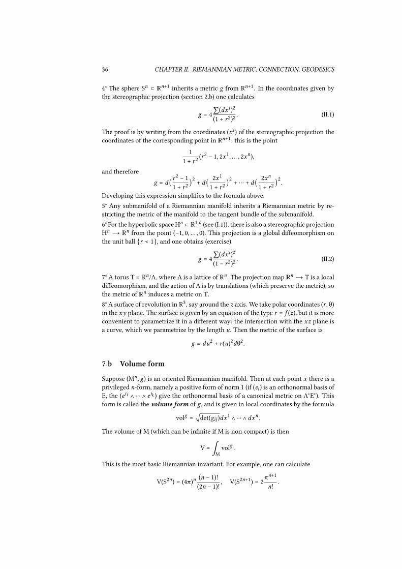
4° The sphere Sn ⊂ ℝn+1 inherits a metric g from ℝ
n+1. In the coordinates given bythe stereographic projection (section 2.b) one calculates
g = 4
∑(dxi)2
(1 + r2)2. (II.1)
The proof is by writing from the coordinates (x i) of the stereographic projection thecoordinates of the corresponding point in ℝ
n+1: this is the point1
1 + r2(r2− 1, 2x
1,… , 2x
n),
and thereforeg = d(
r2− 1
1 + r2)
2
+ d(
2x1
1 + r2)
2
+⋯ + d(
2xn
1 + r2)
2
.
Developing this expression simpli�es to the formula above.5° Any submanifold of a Riemannian manifold inherits a Riemannian metric by re-stricting the metric of the manifold to the tangent bundle of the submanifold.6° For the hyperbolic spaceHn
⊂ ℝ1,n (see (I.1)), there is also a stereographic projection
Hn→ ℝ
n from the point (−1, 0,… , 0). This projection is a global di�eomorphism onthe unit ball {r < 1}, and one obtains (exercise)
g = 4
∑(dxi)2
(1 − r2)2. (II.2)
7° A torus T = ℝn/Λ, where Λ is a lattice of ℝn . The projection map ℝ
n→ T is a local
di�eomorphism, and the action of Λ is by translations (which preserve the metric), sothe metric of ℝn induces a metric on T.8° A surface of revolution in ℝ
3, say around the z axis. We take polar coordinates (r , θ)in the xy plane. The surface is given by an equation of the type r = f (z), but it is moreconvenient to parametrize it in a di�erent way: the intersection with the xz plane isa curve, which we parametrize by the length u. Then the metric of the surface is
g = du2+ r(u)
2dθ
2.
7.b Volume form
Suppose (Mn, g) is an oriented Riemannian manifold. Then at each point x there is a
privileged n-form, namely a positive form of norm 1 (if (ei) is an orthonormal basis ofE, the (ei1 ∧ ⋯ ∧ e
ik ) give the orthonormal basis of a canonical metric on Λ∙E∗). This
form is called the volume form of g, and is given in local coordinates by the formula
volg=
√
det(gij )dx1∧⋯ ∧ dx
n.
The volume of M (which can be in�nite if M is non compact) is then
V =∫M
volg.
This is the most basic Riemannian invariant. For example, one can calculate
V(S2n) = (4π)
n(n − 1)!
(2n − 1)!
, V(S2n+1
) = 2
πn+1
n!
.

8. CONNECTIONS 37
7.c Isometries
De�nition 7.3. A di�eomorphism ϕ ∶ (M, g)→ (N, ℎ) is an isometry if ϕ∗ℎ = g.
The de�nition means ℎϕ(x)
(dxϕ(X), dxϕ(Y)) = gx (X,Y) for all X,Y ∈ TxM, or equival-ently dxϕ is a linear isometry between TxM and T
ϕ(x)N.
Theorem 7.4. The group of isometries of a Riemannian manifold is a Lie group.
We do not prove this theorem, see [Kob95].Example 7.5. 1° The antipodal map x → −x on Sn is an isometry. As a consequence,since ℝP
n is the quotient of Sn by this isometry, the metric of Sn induces a metric onℝP
n .2°The isometries ofℝn consists of orthogonal transformations and translations: Isom(ℝn
) =
ℝn⋉ O(n).
3° Isom(Sn) = O(n + 1), and Isom(Hn) = Oo(1, n), where the index means that we
take the subgroup preserving the nap {x0 > 0} of {(x0)2 − (x1)2 − ⋯ (xn)2= 1}. If
we write SO instead of O in these examples, we obtain the orientation-preservingisometries. These two spaces are homogeneous spaces, that is the isometry groupacts transitively. Therefore they are quotient of the isometry group by the isotropygroup of a point:
Sn= O(n + 1)/
O(n), H
n= O0(1, n)/O(n)
.
ForM = ℝn , Sn or Hn , we have written a group which is clearly a group of isometries,
but we have not proved that there is no other isometry. Nevertheless it is easy to seethat these groups have a stronger property than being just homogeneous: actually,for any points x and y and any isometry u ∶ TxM→ TyM, there exists an element ϕof the group such that ϕ(x) = y and Txϕ = u. (This is because the stabilizer of a pointis each time O(n)). We will see later in corollary 10.4 that for a complete connectedRiemannian manifold, there is at most one isometry with given (x, y,ϕ), so this provesthat there is no possible other isometry.
8 Connections
8.a Connections and Christo�el symbols
Here we address the following problem: �nd a way to take derivatives of sectionsof bundles. Indeed, if we consider the section of a bundle in a local trivialization,we can calculate a derivative, but taking another trivialization will result in anotherderivative. What we need is a covariant derivative.More precisely, what do we need ? suppose E is a vector bundle over M, and s is asection of E. Choose a tangent vector X ∈ TxM, we wish to de�ne a derivative of salong X at x , denoted ∇Xs. This should depend only on the value of X at x and belinear in X ∈ TxM, so at the point x the object (∇s)x should belong to
Hom(TxM,Ex ) = T∗
xM ⊗ Ex .

38 CHAPTER II. RIEMANNIAN METRIC, CONNECTION, GEODESICS
If we now take a vector �eld X ∈ Γ(M,TM), then this means that the covariant de-rivative ∇s should be a section of the bundle T∗M ⊗ E, that is the bundle of 1-formswith values in E. We denote by Ω1(M,E) the space of sections of T∗M ⊗ E, and moregenerally Ωk
(M,E) = Γ(M,ΛkT∗M ⊗ E).
De�nition 8.1. A connection, or covariant derivative, on a real (resp. complex)vector bundle E over M is a ℝ (resp. ℂ)-linear operator
∇ ∶ Γ(M,E)⟶ Ω1(M,E),
satisfying the following Leibniz rule: if f ∈ C∞(M) and s ∈ Γ(M,E), then
∇(f s) = df ⊗ s + f∇s.
As we have already seen in other contexts, the Leibniz rule implies immediately that∇ is a local operator: if U is an open set, (∇s)|U depends only on s|U. Another way tosay the same thing is to say that ∇ induces as well an operator Γ(U,E) → Ω
1(U,E).
Therefore we can take U to be a coordinate chart on which we have a trivialization ofE and write down explicit formulas. Suppose (x i) are local coordinates and (e1,… , er )
is a local basis of sections of E. De�ne the Christo�el symbols Γbia
by
∇ea = Γb
iadx
i⊗ e
b.
A general section of E writes s = saea and applying Leibniz rule:
∇s = dsa⊗ ea + s
a∇ea
= (
)sa
)xi+ Γ
a
ibsb
)dxi⊗ ea
or, equivalently,
∇ )
)xi
s = (
)sa
)xi+ Γ
a
ibsb
)ea .
Therefore we shall write (in this trivialization)
∇ = d + Γidxi,
where Γi = (Γbia) is a matrix (an endomorphism of E). This tells us that the connection∇is locally given by a 1-form with values in End E. In a more synthetic way, considerings as a column vector, the formula above means
∇s = ds + dxi⊗ Γis.
The 1-form Γ = dxi⊗ Γi (with values in End E) is called the connection 1-form.
Let us see what is happening by a change of trivialization. If we have a new basis (fb)
of E, such that ea = ub
afb, then a section s = s
bfb
has coordinates u−1s in the basis (ea)and therefore in this basis ∇s writes d(u
−1s) + dx
iΓiu
−1s. Coming back to the basis
(fb), we obtain
∇s = u(d(u−1s) + dx
iΓiu
−1s) = ds + ( − duu
−1+ dx
iuΓiu
−1
)s.

8. CONNECTIONS 39
In particular, we see that the matrices (Γ′i) in the basis (f
b) can be expressed as
Γ′
i= −
)u
)xiu−1+ uΓiu
−1. (II.3)
This formula is important, it shows that the Γ’s are not tensorial objects (they do notgive a section of Ω1 ⊗ End E), since the law when we change the basis involves deriv-atives of the transition u. Still, we see from the formula that the di�erence betweentwo connections is tensorial: if we have two connections 1∇ and 2
∇, then by a changeof trivialization the equality (II.3) gives
1Γ′
i−2Γ′
i= u(
1Γi −
2Γi)u
−1,
which means now that 1∇ − 2∇ is tensorial: 1∇ − 2∇ ∈ Ω1(M,End E).This can also be seen directly: using the Leibniz formula for both connections, weobtain immediately that
(1∇ −
2∇)(f s) = f (
1∇ −
2∇)s,
that is the di�erence is C∞(M)-linear, implying that it is tensorial. Conversely, if ∇ isa connection and a ∈ Ω
1(M,End E), it is easy to check that ∇+a is again a connection,
so we have proved:
Lemma 8.2. The space of connections on a given bundle E is an a�ne space with directionΩ1(M,End E).
8.b Examples of connections
1° The tangent bundle Tℝn of ℝn with the trivial connection ∇ = d . This means∇ )
)xi
Xj )
)xj=
)Xj
)xi
)
)xj.
2° Here we introduce the bundle O(−1) over ℂP1. This is the ‘tautological’ bundle
whose �ber over a point x ∈ ℂP1 is the complex line x ⊂ ℂ
2. In homogeneous co-ordinates [z1 ∶ z
2] on ℂP
1 we can write two sections: s1 = (1, z2
z1) and s2 = (
z1
z2, 1) ,
de�ned on the open sets U1 = {z1 ≠ 0} and U2 = {z2 ≠ 0}. One has s1 = z2
z1s2 on U12
so the transition function for the bundle O(−1) is u = z2
z1.
Now we de�ne a connection on O(−1) in the following way: locally we can considera section as a map s ∶ ℂP
1→ ℂ
2 such that s(x) ∈ x , and we de�ne
∇Xs = πx (dx s(X)), (II.4)
where πx is the orthogonal projection on x . If we take a coordinate z on U1 by con-sidering the point [1 ∶ z], then we can write s1(z) = (1, z) and therefore
∇Xs1 = π(1,z)(0,X) =
Xz
1 + |z|2s1.
Similarly, with the same coordinate z,
∇Xs2 = −
X
z(1 + |z|2)
s2.

40 CHAPTER II. RIEMANNIAN METRIC, CONNECTION, GEODESICS
So in the two charts we have the Christo�el symbols Γ = zdz
1+|z|2
and Γ′ = − dz
z(1+|z|2). The
di�erence Γ′ − Γ = − dz
zindeed coincides with −duu−1 since u = z. (The connection
is well de�ned on the whole ℂP1 by the formula (II.4); nevertheless, to de�ne it com-
pletely in trivializations, it remains to check that the formula for ∇s2 in U12 extendsto the whole U2 by taking the coordinate z
′=1
z).
3° If M ↪ ℝN is an immersed submanifold, then much as in the previous example
one can de�ne a connection on TM: consider at each point the tangent space TxM asa subspace of ℝn and denote πTxM the orthogonal projection ℝ
n→ TxM, then one
de�nes∇M
Xs = πTxM
(∇ℝn
Xs), X ∈ TxM. (II.5)
It is easy to check that it is indeed a connection on TM.4° Induced connections: a connection on a vector bundle E induces a connection on E∗,by the rule, for s ∈ Γ(E), σ ∈ Γ(E∗) and X ∈ Γ(TM):
LX⟨σ, s⟩ = ⟨∇E∗
Xσ, s⟩ + ⟨σ,∇
E
Xs⟩. (II.6)
If (ea) is a local basis of sections of E, then the dual basis (ea) is a local basis for E∗,and the duality bracket writes, for s = s
aea and σ = σ
beb ,
⟨σ, s⟩ = σasa.
The equation (II.6) then gives immediately
∇ )
)xi
σ = (
)σa
)xi− Γ
b
ia)ea=
)σ
dxi− Γ
t
iσ.
Therefore the connection 1-form for E∗ is −Γt .5° Suppose we have connections ∇E and ∇F on the vector bundles E and F. Then thereis a naturally induced connection on G = Hom(E, F) = E
∗⊗ F, de�ned similarly: one
requests that if s ∈ Γ(E) and u ∈ Hom(E, F), then
∇F(u(s)) = (∇
Gu)(s) + u(∇
Es). (II.7)
From this it follows quickly that
∇G
)
)xi
u =
)u
)xi+ Γ
F
i◦u − u◦Γ
E
i.
(Remark that for F = ℝ we recover the previous case G = E∗).
More generally, by asking that the Leibniz rule like in (II.7) is true for algebraic opera-tions, one easily extends a connection on E to all associated bundles (tensor products,exterior products).
8.c Metric connections
A metric on a vector bundle E is the smooth data of a de�nite positive quadratic formgx in each �ber Ex (Hermitian form if E is complex). An example we have already seenis a Riemannian metric on the tangent bundle. Another example is the bundle O(−1)

8. CONNECTIONS 41
in section 8.b: each �ber is naturally a complex line of ℂ2 and so inherits a Hermitianmetric from that of ℂ2.If the bundle E has a metric g, we say that a connection ∇ on E is a metric connection(or unitary connection) if for any sections s, t of E and any vector �eld X:
LX(g(s, t)) = g(∇Xs, t) + g(s,∇Xt).
What does it mean on the Christo�el symbols ? suppose that (ea) is a local orthonormalbasis of E, then for all a, b we must have g(∇Xea , eb) + g(ea ,∇Xeb) = 0, whence
{
Γb
ia= −Γ
a
ibif E is real,
Γb
ia= −Γ
a
ibif E is complex.
This condition characterizes the metric connections. It means that the matrices Γitake values in antisymmetric or anti-Hermitian endomorphisms of E. So for exampleit is obvious that the �at connection on Tℝn is a metric connection. We shall denotethe bundle of antisymmetric endomorphisms so(E), and the bundle of anti-Hermitianendomorphisms u(E). So we have proved the following version of lemma 8.2:
Lemma 8.3. The space of metric connections of (E, g) is an a�ne space with directionΓ(Ω
1⊗ so(E)) in the real case, Γ(Ω1 ⊗ u(E)) in the complex case.
Exercises. 1° Check the connection we de�ned on O(−1) is a metric connection.2° The connection induced on TM by an immersion M ↪ ℝ
N (see example 3° in 8.b)is a metric connection for the metric induced from the embedding.3° If we have a metric on E, we can identify E∗ with E using the metric. Therefore wehave two connections on E∗: the connection of E ≃ E∗ and the connection as the dualof E. Prove that these two connections coincide.
8.d Parallel transport
If we have a trivial vector bundle E = M×ℝk orM×ℂk , then all �bers of the bundle areidenti�ed with a �xed vector space ℝ
k or ℂk . But for a general vector bundle E overM, there is no canonical way to identify the �bers of Ex , say with Ex0 for x close tox0. We will see that a connection provides exactly the tool for such an identi�cation.
Lemma 8.4. Suppose that (E,∇) is a vector bundle with connection overM. If we have apath c(t) ∈ M, and a section s(t) ∈ E
c(t)of E over c, then ∇
c(t)s(t) depends only on s(t).
Proof. In a local trivialization over a coordinate chart, let c(t) = (x i(t)) and s has valuesin ℝ
k , then we have the formula
∇cs = xi(
)s
)xi+ Γis) = s + Γcs. (II.8)
The same formula shows that the equation
∇cs = 0 (II.9)

42 CHAPTER II. RIEMANNIAN METRIC, CONNECTION, GEODESICS
is a �rst order linear ordinary di�erential equation on s. Therefore given some initialcondition s(0) one can construct a unique solution of (II.9) along c(t). This leads tothe following de�nition:
De�nition 8.5. Let (E,∇) be a bundle with connection overM. If (c(t))t∈[a,b]
is a path inM, then the parallel transport along c is the application E
c(a)→ E
c(b), s(a)↦ s(b)
obtained by solving the equation (II.9) along c.
The parallel transport Ec(a)
→ Ec(b)
is always a linear isomorphism, since the inverseis obtained by parallel transport along c in the reverse direction. If ∇ is a metricconnection, then the parallel transport is an isometry (this can be seen abstractlyusing the de�nition of a metric connection, or directly from equation (II.8) written inan orthonormal trivialization).
9 Riemannian connection, geodesics
9.a The Levi-Civita connection
If we have a connection de�ned on the tangent bundle TM of M, then there is aninteresting invariant:
Lemma and De�nition 9.1. If ∇ is a connection de�ned on the tangent bundle TM ofM, then
TX,Y ∶= ∇XY − ∇YX − [X,Y]
is tensorial. Therefore it de�nes a 2-form on M with values in TM, called the torsion ofM.
The proof of the lemma is left to the reader, who will also check the following localformula for the torsion:
T = (Γk
ij− Γ
k
ji). (II.10)
In particular, a torsion-free connection (that is, a connection with zero torsion),satis�es the symmetry Γk
ij= Γ
k
jiof its Christo�el symbols.
Theorem and De�nition 9.2. If (M, g) is a Riemannian or pseudo-Riemannian man-ifold, then TM admits a unique torsion-free metric connection, called the Levi-Civitaconnection ofM.
Proof. First the uniqueness: if we have two such connections, then by lemma 8.3 thedi�erence between these connections is a 1-form a = (a
k
ij) with values into antisym-
metric endomorphisms of TM. The torsion free condition gives the symmetry condi-tion a
k
ij= a
k
ji. Now instead of choosing a local coordinate trivialization ( )
)xi) of TM, let
us choose an orthonormal trivialization (ei) of TM, and write a in this trivialization.Then the two conditions write:
ak
ij= −a
j
ik, a
k
ij= a
k
ji.
This immediately implies a = 0, so the two connections are equal.

9. RIEMANNIAN CONNECTION, GEODESICS 43
Now let us consider the existence. For a submanifold of ℝN with the induced metric, itis easy to check that the connection de�ned in example 3° of section 8.b, has vanishingtorsion, so this is the connection we want to construct. For an abstract manifold, onehas the formula
2⟨∇XY,Z⟩ = LX⟨Y,Z⟩ +LY⟨Z,X⟩ −LZ⟨X,Y⟩
+ ⟨[X,Y],Z⟩ − ⟨[X,Z],Y⟩ − ⟨[Y,Z],X⟩. (II.11)
The reader will check that this indeed de�nes a metric torsion-free connection.
The formula (II.11) gives immediately an expression in local coordinates. We have
2gklΓl
ij= 2⟨∇ )
)xi
)
dxj,
)
)xk⟩ =
)gjk
)xi+
)gik
)xj−
)gij
)xk
so thatΓl
ij=
1
2
gkl
(
)gjk
)xi+
)gik
)xj−
)gij
)xk). (II.12)
9.b Geodesics
We will now see how the Levi-Civita connection gives us the correct tool to �nd theequation satis�ed by the curves which minimize the distance between two points xand y . Suppose that c ∶ [a, b]→ M is a path, then its length is
L(c) =∫
b
a
√
g(c(t), c(t))dt.
When there is no ambiguity, we will write more simply L(c) = ∫b
a|c|dt . This is inde-
pendent of the parametrization of c, that is L(c◦ϕ) = L(c) for any di�eomorphism ϕ
from an interval of ℝ to [a, b]. In particular it is easy to change the parametrization sothat c is parametrized by arc length: |c| = cst. We want to analyze the paths realizingthe minimum distance from x to y (which we call minimizing paths), and for thiswe will �nd the critical points of L. We consider a family of paths cs ∶ [a, b] → M
depending on s ∈] − ϵ, ϵ[, and we wish to calculate d
dsL(cs) at s = 0. We turn c into a
map [0, 1]×] − ϵ, ϵ[→ M.We note X = Tc(
)
)t) the tangent vectors to the curves, and N = Tc(
)
)s) the vector
tangent to the deformation. Hence X and N are vector �elds de�ned along c, in thesame sense used in lemma 8.4. In particular, the covariant derivatives of X and N arewell de�ned along X and N. The reader will check that [X,N] still makes sense alongc, and that we have the relations
[X,N] = Tc([
)
)t
,
)
)s]) = 0 (II.13)
∇XN − ∇NX − [X,N] = TX,N. (II.14)
Then one can do the following calculation:
d
ds
L(cs) =
d
ds∫
b
a
|X|dt
=∫
b
a
g(X,∇NX)
|X|
dt

44 CHAPTER II. RIEMANNIAN METRIC, CONNECTION, GEODESICS
because ∇ is torsion-free and using (II.13) and (II.14):
=∫
b
a
g(X,∇XN)
|X|
dt
=∫
b
a
1
|X|(
d
dt
g(X,N) − g(∇XX,N)).
Now up to re-parametrizing c0 by arc length, that is |X|s=0 = cst, we obtain the formulafor the variation of length:
d
ds
||||s=0
L(cs) =
1
|X|( − ∫
b
a
g(∇XX,N)dt + g(X,N)|t=1 − g(X,N)|t=0). (II.15)
Now c0 being a critical point of L among paths from x to y means that for any de-formation cs of c with the same endpoints, the derivative of L(cs) at s = 0 vanishes.This implies that (II.15) must vanish for any normal vector �eld N such that N(a) = 0andN(b) = 0. It follows that if c is parametrized by arc length, then c is a critical pointof L if and only if ∇XX = 0, that is ∇c c = 0.
De�nition 9.3. A path c ∶ [a, b]→ M is called a geodesic if ∇c c = 0.
Remark that the de�nition implies d
dt|c|2= 2⟨c,∇c c⟩ = 0, so a geodesic is always para-
metrized by arc length. We then summarize the above calculation in the following:
Lemma 9.4. A path c ∶ [a, b]→ M parametrized by arc length is a critical point of thelength among paths from c(a) to c(b) if and only if it is a geodesic.
Exercise. Prove that the critical points of the energy
E(c) =∫
b
a
|c|2dt (II.16)
among paths from c(a) to c(b) are exactly the geodesics.
Let us write now the geodesic equation in local coordinates (x i): if c(t) = (x i(t)), thenc = x
i )
)xi
and
∇c c = xj
(
)xi
)xj+ Γ
i
jkxk
)
)
)xi
= (xi+ Γ
i
jkxjxk
)
)
)xi
(II.17)
This is a nonlinear second order di�erential equation on (x i(t)). It has a unique solu-tion on some maximal interval as soon as c(0) and c(0) are given, that is the initialposition and the initial speed.Example 9.5. 1° On ℝ
n , the equation reads x i = 0, so the solutions are lines in ℝn .
2° On Sn ⊂ ℝn+1 the Levi-Civita connection is the projection of the Levi-Civita con-
nection of ℝn+1 (see the proof of theorem 9.2). Then check that the solutions are thegreat circles (draw a picture).3° On H
n⊂ ℝ
1,n , this is similar, the geodesics are the intersections of Hn with thehyperplanes of ℝ1,n .4° On a torusMn
= ℝn/ℤ
n , the projection π ∶ ℝn→ M
n is a local isometry, so it sendsa geodesic of ℝn to a geodesic of Mn . Therefore the geodesics are the projections ofstraight lines in ℝ
n .

9. RIEMANNIAN CONNECTION, GEODESICS 45
9.c Killing �elds
We will now see that symmetries of a Riemannian manifold enable to calculate moreeasily the geodesics. Let us begin by introducing the in�nitesimal version of an iso-metry.
Lemma and De�nition 9.6. A vector �eldX on a Riemannian manifold generates a �owof isometries if and only if for any vector �elds Y and Z one has
⟨∇YX,Z⟩ + ⟨∇ZX,Y⟩ = 0.
Such a vector �eld is called a Killing �eld.
Proof. The vectorX generates a �ow (ϕt ) of di�eomorphisms, and d
dtϕ∗
tg =
d
dϵ|ϵ=0ϕ
∗
t+ϵg =
d
dϵ|ϵ=0ϕ
∗
tϕ∗
ϵg = ϕ
∗
tLXg, so ϕt is a �ow of isometries (ϕ∗
tg = g) if and only if LXg = 0.
Now using the properties of the Levi-Civita connection:
(LXg)(Y,Z) = LX(g(Y,Z)) − g(LXY,Z) − g(Y,LXZ)
= g(∇XY − [X,Y],Z) + g(Y,∇XZ − [X,Z])
= g(∇YX,Z) + g(Y,∇ZX).
Remark 9.7. It follows from the de�nition, or from a direct calculation, that the bracketof two Killing vector �elds is again a Killing vector �eld, so the space of Killing vector�elds is an algebra for the bracket. This algebra turns out to be the Lie algebra of theisometry group.
Lemma 9.8. If X is a Killing vector �eld and c a geodesic, then ⟨c,X⟩ is constant alongc.
Proof. One has Lc⟨c,X⟩ = ⟨c,∇cX⟩ = 0 (the �rst equality by the geodesic equation,the second by the Killing condition).
The quantity ⟨c,X⟩ is preserved along a geodesic, it is a �rst integral of the geodesicequation. This is useful for �nding the solutions of the geodesic equation when themetric has symmetries, and we shall now give an example.Example 9.9. Suppose we have a surface of revolution, with metric g = du
2+ r(u)
2dθ
2
(see example 7.2). The rotation vector X =)
)θgenerates the �ow of rotations of the
surface, and is therefore a Killing �eld. Then our �rst integral says immediately thatalong a geodesic c, the quantity r
2 θ is a constant, say C. On the other hand, if we
suppose c parametrized by arc length, then u2+ r
2 θ2= 1. Therefore we obtain the
system
θ =
C
r2, u =
√
1 −
C2
r2. (II.18)
The geodesic equation is now reduced to a system of �rst order di�erential equations,which is completely integrable (one can solve it). Two special kinds of solutions areinteresting:

46 CHAPTER II. RIEMANNIAN METRIC, CONNECTION, GEODESICS
• C = 0, then u(t) = t and θ = cst: these are the meridians;
• u(t) = cst = u0, then C = u0 and θ =
1
r(u0): there are horizontal circles, but they
are geodesics if and only if dr
du|u=u0
= 0. Question: why ? and why do we �ndsolutions which are not geodesics ?
Exercise. On the 2-sphere S2 we consider the metric of revolution
g =
(1 + f (z))2
1 − z2
dz2+ (1 − z
2)dθ
2.
Show that if f is an odd function (f (−z) = −f (z)), then all geodesics of g are circles(Zoll, 1903).
10 Exponential map
10.a Exponential map and injectivity radius
Let (Mn, g) be a Riemannian manifold. Let x ∈ M, X ∈ TxM, and γ be the geodesic
such that γ(0) = x and γ(0) = X. Then we de�ne
expx(X) = γ(1). (II.19)
So expx
is a map from some subset of TxM to M. Remark that if X is tangent to thegeodesic γ(t) and λ ∈ ℝ, then λX is tangent to the geodesic γ(λt), and it follows that
expx(λX) = γ(λ). (II.20)
Since the geodesic γ(t) exists at least for small t , we see that expx(λX) is well de�ned
for small enough λ. Varying X, it follows that expx
is de�ned on some open neigh-borhood of the origin in TxM.Taking the derivative of (II.20) with respect to λ at λ = 0, we see that d0 expx (X) = X,and therefore
d0 expx= 1TxM
. (II.21)
It follows that expx∶ TxM→ M is a local di�eomorphism on a neighborhood of the
origin. Now restrict expx
on an open set U ⊂ TxM on which it is a di�eomorphismonto an open set V ⊂ M, and consider
exp−1
x∶ V⟶ U ⊂ TxM ≃ ℝ
n. (II.22)
This gives a canonical local coordinate chart for M (given the Riemannian metric g),and the coordinates obtained in this way are called normal coordinates.An important notion in Riemannian geometry is the injectivity radius: the injectiv-ity radius at x is the supremum of all r > 0 such that exp
xis a di�eomorphism on
a ball of radius r , and the injectivity radius of M is the in�mum for all x ∈ M of theinjectivity radius at the point x .

10. EXPONENTIAL MAP 47
10.b Normal coordinates
Let us write the metric in normal coordinates: g = gijdxidx
j . Since d0 expxis the
identity, it follows thatgij (0) = δij . (II.23)
In these coordinates, the straight rays from the origin are geodesics:
∇ )
)r
)
)r
= 0. (II.24)
From this equation used at the origin, it follows that ∇ )
)xi
)
)xj(0) = 0 and therefore all
the Christo�el symbols vanish at the origin:
Γk
ij(0) = 0. (II.25)
Finally,)gij
)xk= ⟨∇ )
)xk
)
)xi,
)
)xj⟩ + ⟨
)
)xi,∇ )
)xk
)
)xj⟩
which vanishes at the origin, so it follows that
gij = δij + O(r2). (II.26)
This means that in normal coordinates, the metric is approximated up to second orderby the Euclidean metric ∑(dx
i)2. As we shall see later, it is not possible in general to
obtain a better approximation, because the second derivatives of the coe�cients gijcan be interpreted as curvatures of the metric.Example 10.1. 1° In ℝ
n , one has expx(X) = x + X since the geodesics are the straight
lines. The injectivity radius is +∞.2° In S
n , in the stereographic projection from the north pole, the geodesics issuedfrom the south pole become straight lines, but the velocity in the coordinates is notconstant, see formula (II.1). To obtain the normal coordinates, it is therefore su�cientto re-parametrize each ray by arc length: this gives the change of coordinates ρ =
2 arctan r (so ρ < π), and the formula
g = dρ2+ sin
2(ρ)g
sn−1 . (II.27)
The injectivity radius is π.3° Similarly prove that the hyperbolic metric can be written in normal coordinates as
g = dρ2+ sinh
2(ρ)g
Sn−1 . (II.28)
The injectivity radius is +∞.
Lemma 10.2 (Gauss). If γ(t) is a ray issued from γ(0) = x , and Y ∈ TxM is orthogonalto γ(0), then d
t γ(0)exp
x(Y) ⟂ γ(t) = d
t γ(0)exp
x(γ(0)).
This means that despite the fact that the exponential map is not an isometry, theorthogonality with the rays is preserved.

48 CHAPTER II. RIEMANNIAN METRIC, CONNECTION, GEODESICS
Proof. We use the formula (II.15) for the variation of the length. Note X = γ(0), andconsider a family of geodesics (γs(t))t∈[0,T] issued from x , on a �xed interval [0,T],such that γ0 = γ, |γs(0)| = |X| and d
dsγs |s=0 = Y (this is possible since Y ⟂ X). Then
L(γs) = T|X| is constant, so the formula for the variation of the length gives us
0 =
⟨X,N⟩
|X|
, with N =
dγs(T)
ds
||s=0
.
But N is exactly dTγ(0)
expx(Y) and we get the lemma.
This lemma has several important consequences. First it tells us that in normal co-ordinates, the rays from the origin are orthogonal to the concentric spheres, whichimply that
g = dr2+ gr , gr = r
2gSn−1 + O(r
4), (II.29)
with gr a family of metrics on the sphere Sn−1. For the Euclidean metric gr = r2gSn−1 ,
for the sphere and the hyperbolic space see the formulas (II.27) and (II.28).The second consequence, which follows immediately from (II.29), is that on a ballB ⊂ M on which exp is a di�eomorphism, then for any x ∈ B the shortest path from0 to x is the geodesic from 0 to x , and it is unique. This expresses the fact that thegeodesics are locally minimizing.The third consequence is that small balls are convex: for any x , for r small enough,any two points of the ball B(x, r) are joined by a geodesic which is the unique shortestpath between these two points. The proof is left as an exercise.Fourth and �nal consequence is that any minimizing path between two points is asmooth geodesic. This follows immediately from the fact geodesics are locally minim-izing.
10.c Hopf-Rinow theorem
On a Riemannian manifold (M, g) we have a natural distance
d(p, q) = inf L(path from p to q).
We say that (M, g) is a complete Riemannian manifold if the metric space (M, d) iscomplete. In general a Riemannian manifold is not complete: for example ℝ
n⧵ {0} is
not complete, since a ray going towards the origin must stop after �nite time.
Theorem 10.3 (Hopf-Rinow). Let (M, g) be a connected Riemannian manifold. Thenthe following are equivalent:
1. (M, g) is complete;
2. for any x ∈ M, expxis de�ned on TxM;
3. there exists x ∈ M, such that expxis de�ned on TxM.
If (M, g) is complete, then any two points ofM can be joined by a minimizing geodesic.

10. EXPONENTIAL MAP 49
Proof. 1. ⇒ 2. If one has a geodesic c de�ned on a maximal interval [0,T[ and T
is �nite, then because it is parametrized by arc length and M is complete, it followsthat c(t) has a limit at t = T. The derivative c also converges because |c| = 1 andthe sphere is compact (this is not true in pseudo-Riemannian geometry). Since thegeodesic equation is a second order ODE, it follows that one can extend a bit c beyondT. So T = +∞.3. ⇒ (every point of M can be joined to x by a minimizing geodesic). So �x y ∈ M,we shall construct a geodesic from x to y of length d(x, y). Let S
δ(x) ⊂ M the sphere
of (small) radius δ > 0 around x , then there exists z1 ∈ Sδ(x) such that d(x, y) =
d(x, z1) + d(z1, y). Let c be the geodesic ray from x passing through z1, we shall provethat c(d(x, y)) = y . Let
I = {t > 0, d(x, c(t)) + d(c(t), y) = d(x, y)}.
It is clear that δ ∈ I and I is closed. Let T ∈ I, and suppose that T < d(x, y). Again forsmall ϵ > 0 there exists z2 ∈ Sϵ(c(T)) such that
d(c(T), y) = d(c(T), z2) + d(z2, y).
Then it follows that
d(x, z2) > d(x, y) − d(z2, y) = d(x, c(T)) + d(c(T), y) − d(z2, y)
> d(x, c(T)) + d(c(T), z2)
therefore d(x, z2) = d(x, c(T)) + d(c(T), z2). This implies that the path c from x toc(T) followed by the geodesic from c(T) to z2 is a minimizing path, and therefore isa smooth geodesic: so z2 is on the geodesic c, meaning z2 = c(T + ϵ) so I is open in[0, d(x, y)]. This �nally proves that d(x, y) ∈ I.3. ⇒ 1. If (xi) is a Cauchy sequence, then by the previous statement one has xi =
expx(Xi) with |Xi | = d(x, xi). Since (xi) is bounded, the sequence (Xi) is bounded so
some subsequence converges: Xi′ → X and xi → exp
x(X).
An isometry between Riemannian manifolds M and N sends the metric of M to themetric ofN, and therefore preserves all associated objects, in particular the Levi-Civitaconnection. The image of a geodesic by an isometry is therefore a geodesic: if f ∶
M→ N is an isometry, then
f (expM
xX) = exp
N
f (x)dx f (X)
where expM exists. In particular, if M is complete, by the Hopf-Rinow theorem expM
x
is well de�ned on TxM and therefore the LHS with x �xed and X ∈ TxM determinesf . We deduce:
Corollary 10.4. Suppose f1, f2 ∶ M → N are isometries between connected completeRiemannian manifolds. If for some x ∈ M one has f1(x) = f2(x) and dx f1 = dx f2, thenf1 = f2.

50 CHAPTER II. RIEMANNIAN METRIC, CONNECTION, GEODESICS

Chapter III
Curvature
11 Curvature and integrability
11.a Horizontal distribution
Let π ∶ E→ M be a vector bundle over M with a connection ∇, and x ∈ M. We haveseen in section 8.d that if we have a path (c(t))
t∈[0,1]in M and an initial value s0 ∈ Ex ,
then c can be lifted to a path s in E such that ∇cs = 0.Actually there is an in�nitesimal version of this process: if X = c(0) ∈ TxM, then wede�ne the horizontal lift of X at s0 ∈ Ex to be
X =
ds
dt
||t=0
. (III.1)
We claim that X ∈ Ts0E does not depend of the choice of c, so it depends only of X.
One way to see that is by calculating X in a local trivialization (e1,… , er ) of E, over acoordinate open set U of M, with coordinates (x i). Therefore locally
E|U ≃ U × ℝr
with coordinates (x i , sa)i=1,…,n, a=1,…,r , and the corresponding vector �elds )
)xi
and )
)sa .
Observe that the later ones are tangent to the �bers of E. The connection is written∇ = d + Γ, where Γ is a 1-form with values in End E. From equation (II.8) we obtains(0) = −ΓXs0 and therefore
X = (X, −ΓXs0). (III.2)
For example for X = )
)xi, noting s0 = s
aea , we obtain
X = (
)
)xi, −Γis0) =
)
)xi− Γ
a
ibsb
)
)sa.
.
De�nition 11.1. The horizontal distribution of (E,∇) at each s0 ∈ E is the vectorspace of horizontal lifts {X,X ∈ T
π(s0)M} ⊂ Ts0
E.
51

52 CHAPTER III. CURVATURE
At each point s ∈ E over x ∈ M we have the tangent space to the �ber: Ex ⊂ TsE (thevertical space), and the horizontal distribution (which will be denoted Hs), so that
TsE = Ex ⊕ Hs . (III.3)
We see that the connection ∇ enables to choose a canonical supplementary subspaceto Ex in each tangent space TsE. (This choice actually characterizes ∇). From for-mula (III.2) it follows that at 0 the horizontal distribution coincides with the tangentspace to the zero section {(y, 0), y ∈ M}. From this point of view, the parallel trans-port is interpreted as transporting s over a path c in M by following the horizontaldistribution.
11.b Integrability and curvature
We shall now study the integrability of the horizontal distribution of a connection ∇.Suppose it is integrable, therefore for a small enough open set V ⊂ E containing agiven point (x, 0) we can suppose that V = L × W with L ⊂ ℝ
n and W ⊂ ℝr , and the
leaves of H are the L × {s}. Now consider the application f ∶ V→ M ×W de�ned by
f (l, w) = (π(l, w), w).
Since the leaf L × {0} is just (an open set of) M itself, the di�erential at (x, 0) is anisomorphism. By the inverse function theorem, f is a di�eomorphism from a smalleropen set V′ to an open set of M ×W that we choose of the form U ×W, where U ⊂ M
is a small open set containing x . So we now obtain via f a di�eomorphism
V′≃ U ×W
such that
• the leaves of H are still of the form {y} × W ;
• furthermore in these new coordinates p(y, w) = y .
Here W parametrizes the leaves, it can be identi�ed to the open subset {x} ×W of the�ber Ex .Because the horizontal distribution is preserved by the homotheties s ↦ λs (seeequation (III.2)), this decomposition extends to the whole inverse image π−1(U):
E|U = U × Ex = U × ℝr (III.4)
and the horizontal leaves are obtained by �xing a point on the factor ℝr , therefore theparallel transport in E is given by the identity of ℝr .Here one must be careful that the identi�cation E|U = U × ℝ
r is a priori only a dif-feomorphism, with an identi�cation of ℝr with the �ber at x . But since the paralleltransport between two points of U is given by the identity on the factor ℝr , and theparallel transport acts by linear isomorphisms, we see that over any y the resultingdi�eomorphism Ey = {y}×ℝ
r is actually a linear isomorphism. This means that (III.4)is a local trivialization of E as a vector bundle. Then the equation (III.2) gives immedi-ately Γ = 0 everywhere in this trivialization, so ∇ is the trivial connection ∇ = d . Wehave proved:

11. CURVATURE AND INTEGRABILITY 53
Lemma 11.2. The horizontal distribution of ∇ is integrable if and only if E admits localtrivializations in which ∇ is trivial.
Remark that if ∇ is a metric connection, then the local trivializations can be supposedto be orthonormal, since the parallel transport preserves the metric.In view of Frobenius theorem 5.4, the condition of integrability of the horizontal dis-tribution is equivalent to its involutivity. Let us study the condition in a local trivial-ization as above. Suppose X and Y are two local vector �elds on M, then
[X, Y] = [X − Γa
Xbsb
)
)sa,Y − Γ
a
Ybsb
)
)sa]
= [X,Y] + ( −LXΓa
Yb+LYΓ
a
Xb+ Γ
a
XcΓc
Yb− Γ
c
XbΓa
Yc)sb
)
)sa
using the di�erential of the 1-form Γa
b∶ X↦ Γ
a
Xb:
=[X,Y] − (dΓ
a
b(X,Y) + Γ
a
XcΓc
Yb− Γ
c
XbΓa
Yc)sb
)
)sa.
We can rewrite this formula in a more concise way:
[X, Y](s) =[X,Y](s) − ((dΓ)X,Ys + [ΓX, ΓY]s)
=[X,Y](s) − FX,Ys, (III.5)
where we de�neFX,Y = (dΓ)X,Y + [ΓX, ΓY]. (III.6)
This is a 2-form with values in End E, so an element ofΩ2(End E). From equation (III.5)it is clear that it does not depend on the trivialization, but this can also be checkeddirectly: if we choose a di�erent trivialization (ea) = ϕ(fb), then by (II.3) we have thetransformation Γ→ ϕ◦Γ◦ϕ
−1− dϕ◦ϕ
−1, and the reader can check that F→ ϕ◦F◦ϕ−1.
De�nition 11.3. The curvature of the connection ∇ is the 2-form with values in End Ede�ned locally by the formula (III.6).
Recall that if the connection is metric, then Γ is a 1-form with values in so(E) or u(E) inan orthonormal trivialization, and one can read from formula (III.6) that F is a 2-formwith values in the same bundle.Example 11.4. If we take the line bundle O(−1) over ℂP
1, with the connection Γ =
zdz
1+|z|2
constructed in section 8.b, then the brackets in (III.6) vanish since we have onlya line bundle, and we get
FO(−1)
= −
dz ∧ dz
(1 + |z|2)2=
2idx ∧ dy
(1 + x2+ y
2)2,
which is a 2-form with values in iℝ = u1. (As we shall see later, the �rst Chern numberof O(−1) is i
2π∫ℂP
1 F = −1).
De�nition 11.5. A connection is �at if its curvature vanishes.
Since the vanishing of the curvature is equivalent to the involutivity of the horizontaldistribution, lemma 11.2 implies that ∇ is �at if and only if E has local trivializationsin which ∇ is the trivial connection: ∇ = d .In the special case of the Levi-Civita connection, we obtain:

54 CHAPTER III. CURVATURE
Lemma 11.6. If (Mn, g) is a Riemannian manifold, then its Levi-Civita connection is �at
if and only if near any point there exist local coordinates (x i) such that g = ∑(dxi)2.
Proof. If the Levi-Civita connection on TM is �at, then near each point we have anorthonormal basis (X1,… ,Xn) of parallel vector �elds: ∇Xi = 0. In particular, since ∇is torsion-free, one has [Xi ,Xj] = ∇Xi
Xj − ∇XjXi = 0. From the proof of lemma 5.3, it
follows that there exists local coordinates such that Xi =)
)xi.
11.c Second derivatives and curvature
Here we present another de�nition of the curvature, less geometric but of equal im-portance. Suppose (E,∇) is a �ber bundle.
Lemma and De�nition 11.7. If X and Y are vector �elds and s is a section of E, then
FX,Ys = ∇X∇Ys − ∇Y∇Xs − ∇[X,Y]s
is tensorial inX, Y and s, and de�nes a 2-form Fwith values in End E called the curvatureof E.
The proof is left to the reader. In a trivialization, ∇ = d + Γidxi , and one can calculate
directlyFij =
)Γj
)xi−
)Γi
)xj+ [Γi , Γj] (III.7)
which is the same result as in equation (III.6), so we de�ned the same object.This point of view will be used later in various calculations, in particular to establishthe di�erential Bianchi identity 16.2.
12 Riemannian curvature
12.a Symmetries of the Riemannian curvature
The Levi-Civita connection satis�es additional properties, which make sense only forconnections on the tangent bundle. In general we will denote the curvature of theLevi-Civita connection by R, so R is an element of Ω2(M, o(TM)).
Lemma 12.1 (Bianchi identity). The Levi-Civita connection R of a Riemannian man-ifold satis�es
RX,YZ + RY,ZX + RZ,XY = 0.
Proof. This quantity is
∇X∇YZ − ∇Y∇XZ − ∇[X,Y]Z + ∇Y∇ZX − ∇Z∇YX−∇[Y,Z]X
+ ∇Z∇XY−∇X∇ZY − ∇[Z,X]Y
The three underlined terms give [X, [Y,Z]], and gathering the other terms similarly,we get
[X, [Y,Z]] + [Y, [Z,X]] + [Z, [X,Y]]
which vanishes by the Jacobi identity. (This proof extends to any torsion-free con-nection).

12. RIEMANNIAN CURVATURE 55
Corollary 12.2. The Riemannian curvature satis�es
⟨RX,YZ,T⟩ = ⟨RZ,TX,Y⟩.
Therefore R de�nes a symmetric endomorphism ofΛ2TM called the curvature operator.
The proof is left to the reader, who should play with the Bianchi identity and the factthat RX,Y is an anti-symmetric endomorphism.This gives symmetries satis�ed by the Riemannian curvature. If we take an orthonor-mal basis of vector �elds (X1,… ,Xn), we can write down the curvature as R = (R d
abc),
with ab the indices of the 2-form, and cd that of the anti-symmetric endomorphism.Then we have the following symmetries:
Rd
abc= −R
d
bac, R
c
abd= −R
d
abc, R
b
cda= R
d
abc.
12.b Sectional curvature
From these symmetries we see for example that in dimension 2, the curvature hasonly one coe�cient K = R 1
122which is the Gauss curvature of the surface. In higher
dimension, one de�nes analogous 2-dimensional curvatures in the following way:
De�nition 12.3. Let (M, g) be a Riemannian manifold, and P ⊂ TxM a 2-plane. Onede�nes the sectional curvature of the plane P as the number
K(P) =
g(RX,YY,X)
g(X,X)g(Y,Y) − g(X,Y)2
for any basis (X,Y) of P.
It is easy to check that the de�nition does not depend on the basis (X,Y). Also thede�nition still makes sense in pseudo-Riemannian manifolds, provided that the de-nominator does not vanish.One can prove that the data of the sectional curvatures of all 2-planes in TxM com-pletely determines the curvature tensor at the point x .Example 12.4. 1° The curvature of the �at ℝn vanishes and therefore all the sectionalcurvatures vanish.2° For the sphere Sn , we �rst observe that the isometry group SO(n + 1) is transitiveon 2-planes: indeed it is transitive on the points of Sn , and the isotropy group of apoint is SO(n) which acts transitively on 2-planes of ℝn . Since the curvature and thesectional curvatures are canonically de�ned from the metric, they are preserved byisometries and it follows that all the sectional curvatures of Sn equal a �xed constant(+1, as we shall see later).3° Similarly the hyperbolic space Hn has constant sectional curvature.4° The sectional curvatures of λ2g, where λ is a positive number, are related to that ofg by the relation
Kλ2g=
1
λ2Kg. (III.8)
This comes immediately from the fact that g and λ2g have the same Levi-Civita con-nection, and therefore the same curvature tensor R. The formula corresponds to theidea that if we make a sphere very big (λ big), then its curvature becomes small, thatis it becomes almost �at. Indeed the earth looks locally very �at !

56 CHAPTER III. CURVATURE
13 Second fundamental form
13.a Covariant derivative and second fundamental form
Suppose that (Mn, g) is an oriented Riemannian manifold, and Nn−1
⊂ M is a subman-ifold oriented by the normal vector n. Similarly to the case of submanifolds of ℝn , itis easy to check that the Levi-Civita connection of N is
∇N= π◦∇
M, (III.9)
where π ∶ TxM→ TxN is the orthogonal projection. Therefore, for two vector �eldsX, Y on N, the covariant derivative ∇M
XY decomposes as
∇M
XY = ∇
N
XY + I(X,Y)n. (III.10)
Actually, in the pseudo-Riemannian case, it will be useful to use the following nor-malization:
∇M
XY = ∇
N
XY + I(X,Y)
n
⟨n, n⟩
. (III.11)
Developing the torsion-free condition ∇MXY−∇
M
YX = [X,Y]with (III.10), we obtain the
symmetry conditionI(X,Y) = I(Y,X). (III.12)
A priori the formula (III.10) de�nes I(X,Y) as a tensorial object only with respect toX. Then the symmetry (III.12) proves that it is tensorial also with respect to Y (thiscan also be checked directly). We can now state:
De�nition 13.1. The formula I(X,Y) = ⟨∇M
XY, n⟩ de�nes a symmetric 2-tensor on N,
called the second fundamental form of N.
Directly from the de�nition, using the properties of ∇M, one also gets:
I(X,Y) = −⟨∇M
Xn,Y⟩. (III.13)
This gives another formula for the second fundamental form: I = −∇Mn.
13.b Curvature and second fundamental form
There is an application ϕ ∶ ℝ × N→ M, de�ned by
ϕ(r , x) = expx(rn).
(If M is not complete, then ϕ may be de�ned only on an open subset of ℝ × N). Thismeans that from each point x ∈ N we draw the geodesic from x which is orthogonalto N, and we parametrize it by its arc length r .The di�erential of ϕ at a point (0, x) is d
(0,x)ϕ(r ,X) = rn + X, so it is an isomorphism
ℝ × TxN → TxM. It follows that ϕ is a di�eomorphism from a neighborhood of{0} ×N ⊂ ℝ ×N onto a neighborhood of N ⊂ M (say, if N is compact, or at least locallynear any point of N).
Lemma 13.2. The geodesics normal to N are orthogonal to the hypersurfaces ϕ({r} ×N).

13. SECOND FUNDAMENTAL FORM 57
Proof. This is a version of Gauss lemma 10.2, the proof is similar.
It follows that on the open set where ϕ is a di�eomorphism, one has
ϕ∗g = dr
2+ gr , gr metric on N. (III.14)
The normal vector n can then be extended to a neighborhood of N as ϕ∗ ))r . If X is avector �eld on N, one can extend it to a neighborhood of N as being independent ofthe ℝ variable in the product ℝ × N; equivalently, this is the unique extension so that[n,X] = 0. Choose two vector �elds X, Y on N and extend them in this way: then from(III.13) one deduces
I(X,Y) = −⟨∇nX,Y⟩ + ⟨[n,X],Y⟩ = −⟨∇
nX,Y⟩;
by symmetry we get
I(X,Y) = −
1
2(⟨∇n
X,Y⟩ + ⟨∇nY,X⟩) = −
1
2
Ln⟨X,Y⟩.
This proves the formula:I = −
1
2
)gr
)r
||r=0
, (III.15)
which gives a concrete formula to calculate I.Often we will need to consider I as a symmetric endomorphism of N rather than aquadratic form: therefore we de�ne the Weingarten endomorphism A by the for-mula
I(X,Y) = g(A(X),Y), A(X) = −∇Xn, (III.16)so that we have the formula
A = g−1I = −
1
2
g−1)g
)r
. (III.17)
Lemma 13.3. If X and Y are two vectors of N, one has the formulas
KM(X ∧ Y) = K
N(X ∧ Y) − ⟨n, n⟩
I(X,X)I(Y,Y) − I(X,Y)2
⟨X,X⟩⟨Y,Y⟩ − ⟨X,Y⟩2; (III.18)
KM(X ∧ n) =
LnI(X,X) + |AX|
2
⟨X,X⟩⟨n, n⟩
. (III.19)
In the second formula, A is the Weingarten endomorphism of the hypersurfaces {r} × N.
It is important to note that this lemma is written for a pseudo-Riemannian manifold:that is why we kept ⟨n, n⟩ which may equal −1.
Proof. We only deal with the Riemannian case, and let the reader check the signs inthe pseudo-Riemannian case.Let X and Y be tangent vectors to N at the point x . We can extend X and Y so that[X,Y] = 0. Let Z, T be vector �elds on N, and denote ∇ the connection of M and ∇Nthat of N. Then
⟨∇X∇YZ,T⟩ = ⟨∇X(∇N
YZ + I(Y,Z)n),T⟩
= ⟨∇N
X∇N
YZ + I(Y,Z)∇Xn,T⟩
= ⟨∇N
X∇N
YZ,T⟩ − I(Y,Z)I(X,T).
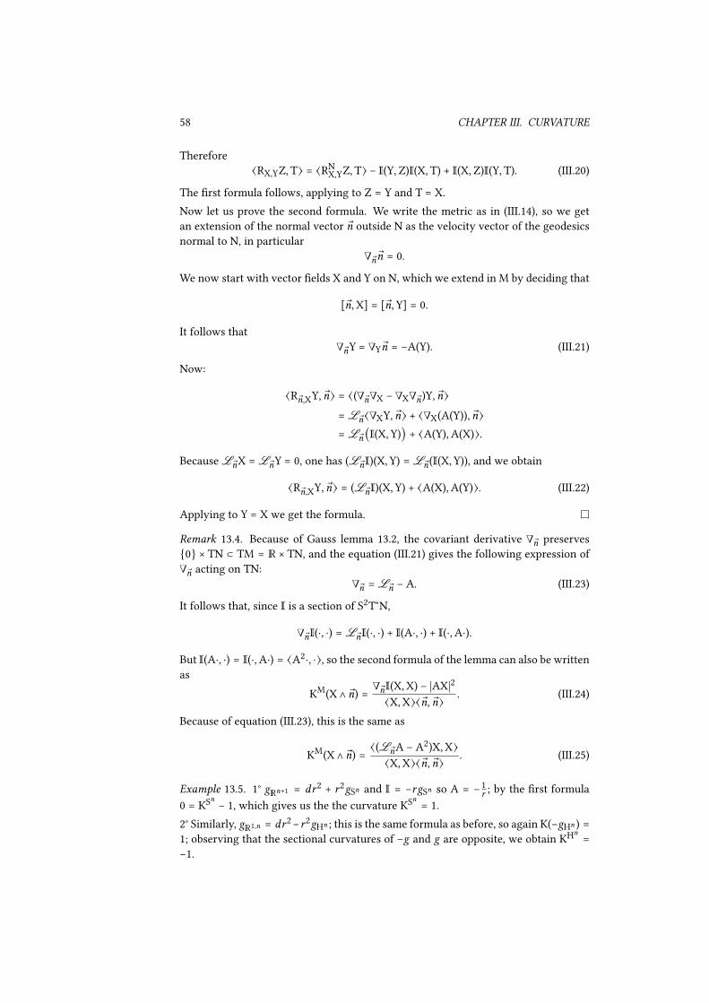
58 CHAPTER III. CURVATURE
Therefore⟨RX,YZ,T⟩ = ⟨R
N
X,YZ,T⟩ − I(Y,Z)I(X,T) + I(X,Z)I(Y,T). (III.20)
The �rst formula follows, applying to Z = Y and T = X.Now let us prove the second formula. We write the metric as in (III.14), so we getan extension of the normal vector n outside N as the velocity vector of the geodesicsnormal to N, in particular
∇nn = 0.
We now start with vector �elds X and Y on N, which we extend in M by deciding that
[n,X] = [n,Y] = 0.
It follows that∇nY = ∇Yn = −A(Y). (III.21)
Now:
⟨Rn,XY, n⟩ = ⟨(∇
n∇X − ∇X∇n
)Y, n⟩
= Ln⟨∇XY, n⟩ + ⟨∇X(A(Y)), n⟩
= Ln(I(X,Y)) + ⟨A(Y),A(X)⟩.
Because LnX = L
nY = 0, one has (L
nI)(X,Y) = L
n(I(X,Y)), and we obtain
⟨Rn,XY, n⟩ = (L
nI)(X,Y) + ⟨A(X),A(Y)⟩. (III.22)
Applying to Y = X we get the formula.
Remark 13.4. Because of Gauss lemma 13.2, the covariant derivative ∇n
preserves{0} × TN ⊂ TM = ℝ × TN, and the equation (III.21) gives the following expression of∇n
acting on TN:∇n= L
n− A. (III.23)
It follows that, since I is a section of S2T∗N,
∇nI(⋅, ⋅) = L
nI(⋅, ⋅) + I(A⋅, ⋅) + I(⋅,A⋅).
But I(A⋅, ⋅) = I(⋅,A⋅) = ⟨A2⋅, ⋅⟩, so the second formula of the lemma can also be written
asKM(X ∧ n) =
∇nI(X,X) − |AX|
2
⟨X,X⟩⟨n, n⟩
. (III.24)
Because of equation (III.23), this is the same as
KM(X ∧ n) =
⟨(LnA − A
2)X,X⟩
⟨X,X⟩⟨n, n⟩
. (III.25)
Example 13.5. 1° gℝn+1 = dr
2+ r
2gSn and I = −rgSn so A = −
1
r; by the �rst formula
0 = KSn
− 1, which gives us the the curvature KSn = 1.2° Similarly, g
ℝ1,n = dr
2−r
2gHn ; this is the same formula as before, so again K(−gHn ) =
1; observing that the sectional curvatures of −g and g are opposite, we obtain KHn
=
−1.

13. SECOND FUNDAMENTAL FORM 59
13.c Surfaces in ℝ3
If we have a surface S ⊂ ℝ3, then the two eigenvalues λ1 and λ2 of I are called the
principal curvatures of S. The �rst equation gives us the well-known formula forthe Gauss curvature:
KS= λ1λ2.
The principal curvatures depend on the embedding S ⊂ ℝ3 but the product depends
only on the intrinsic geometry of S: this is the content of the theorem Egregium ofGauss. Also
H = λ1 + λ2
is called the mean curvature. Surfaces withH = 0 are called minimal surfaces: thisis the equation satis�ed by the soap bubbles.Finally, if the surface S is given by an equation z = f (x, y), then the reader will checkthe following explicit formulas: the metric on S is given by
g11 = 1 + ()x f )2, g12 = )x f )y f , g22 = 1 + ()y f )
2
the normal vector isn =
(−)x f , −)y f , 1)
√
1 + ()x f )2+ ()y f )
2
,
from which one deduces the second fundamental form:
I11 =)2
xxf
√
1+()x f )2+()y f )
2, I12 =
)2
xyf
√
1+()x f )2+()y f )
2, I22 =
)2
yyf
√
1+()x f )2+()y f )
2.
It follows that the curvature of S is given by
K =
det(Iij )
det(gij )
=
)2
xxf )
2
yyf − ()
2
xyf )2
1 + ()x f )2+ ()y f )
2.
The geometric meaning is then clear: in particular for K > 0 we get a convex surface.
13.d A geometric interpretation of the curvature
The sectional curvatures of a Riemannian metric g can be seen as coe�cients is theTaylor development of the metric in normal coordinates. Recall that in normal co-ordinates,
exp∗
xg = dr
2+ r
2(gSn−1 + r
2γ +⋯).
Note γ = g−1
Sn−1γ the corresponding endomorphism on TSn−1, then
I ∼ −
1
2
)g
)r
∼ −rgSn−1 − 2r
3γ, A ∼ −
1
r
(1 + r2γ).
Fix a vector X ∈ Sn−1 ⊂ TxM, which we can suppose to be an eigenvector of γ for theeigenvalue γ, then
K(
)
)r
∧ X) =
L )
)r
I(X,X) + g(A2X,X)
g(X,X)
∼
(−1 − 6r2γ) + (1 + 3r
2γ)
1 + r2γ
∼ −3γ.

60 CHAPTER III. CURVATURE
We deduce:g(X,X) ∼ r
2−
1
3
K(
)
)r
∧ X)r4+⋯ (III.26)
For the �at ℝn , one has K = 0 and the geodesics are straight lines. The equation (III.26)means that, at least near the point x , comparing with the straight lines:
• when K > 0 the geodesics get closer (think of the sphere: two great circlesstarting from the same point �nally meet again);
• when K < 0 the geodesics get far away from each other.
K > 0 K < 0
14 Constant curvature metrics
Lemma 14.1. If (Mn, g) has constant sectional curvature, then in normal coordinates
exp∗g coincides with the metric of ℝn , Sn or Hn (up to a multiplicative constant).
Proof. We use normal coordinates around a point x : then g = dr2+ gr , with gr a
metric on Sn−1. The second formula of lemma 13.3, under the form (III.24), gives us
)A
)r
− A2= k, (III.27)
where k is the (constant) sectional curvature. When r → 0 we have the asymptoticbehavior A ∼ −
1
r, and in particular A is invertible near 0. Consider B = A−1, then B
extends at 0 with B(0) = 0 and satis�es)B
)r
= −1 − kB2.
One can solve this ODE and deduce gr :
• if k = 0, then B = −r , A = − 1r
and gr = r2;
• if k > 0, then A = − cot(√
kr)√
k
and gr =sin
2(
√
kr)
k;
• if k < 0, then A = − coth(√
−kr)√
−k
and gr =sinh
2(
√
−kr)√
−k
.
Corollary 14.2. A Riemannian manifold with constant curvature is locally isometricto ℝ
n , Sn or Hn (up to a constant). If moreover the manifold is connected and simplyconnected, then it is exactly ℝ
n , Sn or Hn .
The �rst part of the corollary is an immediate consequence of the lemma. The secondpart is more global and will be proved in the next section.

15. RIEMANNIAN CURVATURE AND TOPOLOGY 61
15 Riemannian curvature and topology
Here we will see how the curvature—more precisely its sign—has in�uence on thetopology of the manifold. This is an important area of research in geometry, andwe give only two basic results, the Cartan-Hadamard theorem and the Bonnet-Myerstheorem.
15.a The conjugacy radius
In section 10 we have seen the notion of injectivity radius—the supremum of the r > 0such that exp
xis a di�eomorphism on the ball of radius r . Here we will use another
notion, the conjugacy radius, that is the supremum of the r > 0 such that expx
isa local di�eomorphism on the ball of radius r . This is equivalent to exp∗
xg being a
metric on the ball of radius r , so we can de�ne alternatively the conjugacy radius atx by
ρconj (x) = inf{r > 0, det(exp∗
xg) vanishes at some point of S(r)}. (III.28)
As in the proof of lemma 14.1, by Gauss lemma we have exp∗xg = dr
2+ gr and on the
ball of radius ρconj (x), one has, for |X| = 1,
⟨(∇ )
)r
A − A2)X,X⟩ = K(
)
)r
∧ X). (III.29)
So for example if K 6 0, then ∇ )
)r
A−A2 6 0 which implies A 6 −
1
rand gr > r
2gSn−1 .
It follows that det(exp∗xg) can never vanish and we obtain the �rst part of:
Corollary 15.1. If K 6 0, then ρconj = +∞. If K 6 k with k > 0, then ρconj > π√
k
.
Proof. It remains to deal with K 6 k: the same proof gives us gr > sin2(
√
kr)
kand
therefore det(exp∗xg) cannot vanish for r < π
√
k
.
15.b The Cartan-Hadamard theorem
Theorem15.2 (Cartan-Hadamard). If (Mn, g) is a complete connected Riemannianman-
ifold with K 6 0, then expx∶ TxM → M is a covering. In particular, if M is simply
connected, thenM is di�eomorphic to ℝn .
Proof. We have just seen that expx
is a local di�eomorphism. It follows that expx∶
(TxM, exp∗
xg) → (M, g) is an isometry. But it is a general fact that any isometry
from a complete space is a covering: denote by f the isometry, then if if r > 0 issmaller than the injectivity radius at y , the inverse image f
−1(B(y, r)) is the disjoint
union of balls of radius r . Indeed, if x ∈ f−1(y) then using the exponential map one
can see immediately that f |B(x,r)
∶ B(x, r) → B(y, r) is a di�eomorphism; and if x ∈f−1(B(y, r)), then there is a geodesic ray in B(y, r) from f (x) to y , say y = exp
f (x)(X),
then f (expx((dx f )
−1(X))) = y therefore x ∈ B(z, r) with z = (dx f )
−1(X).
For constant curvature metrics, we deduce:

62 CHAPTER III. CURVATURE
Proof of corollary 14.2. In the case of negative or zero curvature, this is just the Cartan-Hadamard theorem, and the fact that we have an explicit formula for a constantcurvature metric in normal coordinates.In the case of positive curvature, we can suppose that K = 1. Then by corollary 15.1,the map exp
xis a local di�eomorphism on the ball B(0,π) ⊂ TxM, and since K = 1,
exp∗
xg = dr
2+ sin
2(r)ds
2
Sn−1 on B(0,π).
Since this is exactly the expression of the metric of Sn in normal coordinates, wededuce an isometric map fN ∶ S
n⧵ {S}→ M by the composition
Sn⧵ {S}
exp∗
N
−−−−−→ (B(0,π), dr2+ sin
2(r)ds
2
Sn−1 )
expx
−−−−→ M.
We can do the same thing from another point y = f (p) where p ∈ Sn⧵ {S}, and we
obtain another isometry fp ∶ Sn⧵ {q}→ M, where q is the antipodal point to p, such
thatfp(p) = y = fN(p), dpfp = dpfN.
Since a local isometry sends a geodesic to a geodesic, it then follows that fp and fN
coincide, except maybe on the segment joining q and S. As fp is de�ned on Sn ⧵ {q}and fS on S
n⧵ {N}, it follows that they coincide everywhere, and therefore de�ne
together an isometric map f ∶ Sn→ M, which is therefore a covering. If M is simply
connected, f must be a global di�eomorphism.
15.c The Bonnet-Myers theorem
Theorem 15.3 (Bonnet-Myers). If (Mn, g) is a complete connected Riemannian mani-
fold, satisfying (Bonnet)K > k > 0,
or the weaker hypothesis (Myers)
Ric > (n − 1)k,
then the diameter of M is not bigger than π√
k
. In particular M is compact. Moreoverπ1(M) is �nite.
Here Ric denotes the Ricci tensor, which will be studied in chapter IV. For this the-orem, we just need to know the de�nition:
Ric(X,Y) = Tr(Z↦ RZ,XY). (III.30)
It is a symmetric 2-tensor. In particular, if |X| = 1, we complete X into an orthonormalbasis (X = e1,… , en), and
Ric(X,X) =
n
∑
1
⟨Rei ,XX, ei⟩ =
n
∑
2
K(X ∧ ei). (III.31)
Then it is clear that the �rst hypothesis of the theorem is stronger than the secondone.

15. RIEMANNIAN CURVATURE AND TOPOLOGY 63
Before giving a proof of the theorem, we outline another approach, more in the spiritof what we have just done. Recall that at a point x we have exp∗
xg = dr
2+ gr , with
A = −1
2g−1
r
)gr
)rsatisfying equation (III.29) where exp
xis non degenerate. Taking the
trace of the equation, we obtain
) Tr(A)
)r
−
Tr(A)2
n − 1
> Ric(
)
)r
,
)
)r
) > (n − 1)k > 0,
which implies Tr(A) > −(n − 1)
√
k cot(
√
kr) and det(gr ) 6 (
sin(
√
kr)√
k)
n−1. On eachray from the origin, we see that det(gr ) must vanish at a radius r 6 R with R = π
√
k
,that is d exp
xhas a kernel on each ray at most at distance R. One says that x has a
conjugate point on every geodesic from x at distance at most R. But it is known thata geodesic cannot be minimizing after a conjugate point, and it follows that all pointsof M are at most at distance R from x . The proof of this last fact requires the theoryof Jacobi �elds that will not be developed in these notes, see for example [GHL04].
Proof. So we now turn to the proof of the theorem. It relies on the second variationof arc length: if (cs(t)) is a family of paths de�ned on [a, b], with �xed endpoints, andc0 is a geodesic, then
d2L(cs)
ds
||s=0
=∫
b
a
(|∇c0N|2− ⟨R
c0,NN, c0⟩)dt (III.32)
where N =)c
)sand N is the projection of N orthogonally to c0. The proof of this
formula is similar to that of the �rst variation of arc length (II.15) and is left to thereader.Suppose we have two points x, y ∈ M. By the Hopf-Rinow theorem 10.3, there existsa minimizing geodesic c from x to y , of length L = d(x, y). Now choose vectorsE1,. . . ,En−1 along c0 such that (c,E1,… ,En−1) is a parallel basis of orthonormal vectorsalong c. For i = 1,… , n − 1 choose
Ni = sin(π
t
L
)Ei .
These vectors vanish at the endpoints of [0, L]. Fix i and choose a variation (cs) of cwith �xed endpoints, such that )c
)s|s=0 = Ni . Since c is a minimizing geodesic, we have
d2L(cs )
ds2
|s=0 > 0, and therefore
∫
L
0
|∇cNi |2− ⟨Rc,Ni
Ni , c⟩ > 0.
But ∇cNi =π
Lcos(
πt
L)Ei so after summation over i we obtain
(n − 1)π2
L2 ∫
L
0
cos(πt
L)2 >
∫
L
0
sin(πt
L)2
n−1
∑
1
K(c,Ei) = ∫
L
0
sin(πt
L)2Ric(c, c).
The hypothesis gives (n − 1)π2L2> (n − 1)k so L2 6 π
2
k.
The diameter being �nite implies immediately that M is compact. Also remark thatone can pullback the metric of M on its universal covering M, so M also satis�es thehypothesis: it is therefore compact, which implies that π1(M) is �nite.

64 CHAPTER III. CURVATURE
Remark that the formula (III.32) can be rewritten as
d2L(cs)
ds
||s=0
= −∫
b
a
⟨∇c∇cN + Rc,NN, c⟩dt (III.33)
so the vector �elds satisfying the second order linear ODE ∇c∇cN + Rc,NN = 0 are
exactly the kernel of the Hessian of L. These are the Jacobi �elds alluded to above.
16 Chern-Weil construction
We now pass to a di�erent topic: the construction of topological invariants of a vectorbundle from the curvature of a connection on the bundle. This �rst requires to studymore properties of the connection and the curvature.
16.a Extension of a connection
Let E→ M be a vector bundle with a connection ∇ ∶ Γ(E)→ Ω1(E). In section 6.c we
extended the derivative of functions to the exterior di�erential on forms. In the sameway, we extend ∇ uniquely to an exterior di�erential on E-valued di�erential forms:
d∇∶ Ω
k(E)⟶ Ω
k+1(E) (III.34)
satisfying the Leibniz identity, for α a di�erential form and σ an E-valued di�erentialform:
d∇(α ∧ σ) = dα ∧ σ + (−1)
|α|α ∧ d
∇σ. (III.35)
This extension can be de�ned by the local formula d∇σ = dσ+a∧σ in a trivialization ofE in which ∇ = d +a for an End(E)-valued 1-form a. There is also a formula analogousto lemma 6.3:
(d∇σ)X0,…,Xk
=
k
∑
0
(−1)k∇Xi
(σX0,…,Xi ,…,Xk
)
+ ∑
06i<j6k
(−1)i+jσ([Xi ,Xj],X0,… , Xi ,… , Xj ,… ,X
k). (III.36)
This extension leads to a nice interpretation of the curvature: recall that the exteriordi�erential satis�es d◦d = 0. The curvature is precisely the defect for d∇◦d∇ to vanish:
Lemma 16.1. 1° The curvature F∇, seen as an operator Γ(E)→ Ω2(E), is F∇ = d
∇◦d∇.
2° As an operator Ωk(E)→ Ω
k+2(E), one has F∇ = d
∇◦d∇.
Proof. Let us choose a local trivialization of E, and write the connection ∇ = d+a = d+
aidxi , where each ai is End(E)-valued. Then, for a section s of E, we have d∇s = ds+as
and
d∇(d∇s) = (d + a)(d + a)s
= d(as) + a ∧ ds + a ∧ as
= (da + a ∧ a)s.
This proves the �rst statement. The proof of the second one is similar.

16. CHERN-WEIL CONSTRUCTION 65
We deduce the following important identity:
Proposition 16.2 (di�erential Bianchi identity). The curvature of a connection sat-is�es the identity
d∇F∇= 0.
Remark that F∇ ∈ Ω2(End(E)) so d∇ is the exterior derivative associated to the con-
nection ∇ on End E, and d∇F∇∈ Ω
3(End(E)).
Proof. In this proof let us distinguish ∇ on E and ∇ on End E. Recall that, as a linearoperator on E, for u ∈ Γ(End E) one has ∇u = ∇◦u − u◦∇. Then the reader will checkthat, as operators Γ(E)→ Ω
3(E), one has d ∇F∇ = d
∇◦F∇−F
∇◦d∇. But since F∇ = d
∇◦d∇,
we obtaind∇F∇= d
∇◦d∇◦d∇− d
∇◦d∇◦d∇= 0.
16.b Chern-Weil homomorphism
We �x a ℂr vector bundle E over M. Let P ∶ gl
rℂ ⊗ ⋯ ⊗ gl
rℂ → ℂ a symmetric k-
linear form on glrℂ. As is well-known this is equivalent to giving the homogeneous
polynomial P(A,… ,A) of degree k on glrℂ. We suppose that P is GLrℂ invariant, that
isP(gA1g
−1,… , gA
kg−1) = P(A1,… ,A
k)
for all g ∈ GLrℂ. Di�erentiating at the identity, this is equivalent to
P([X,A1],A2,… ,Ak) +⋯ + P(A1,… ,A
k−1, [X,A
k]) = 0
for all X ∈ glrℂ. A basis of such polynomials is (Tr(Ak
))k=0,…,r
.If α1, . . . , α
kare di�erential forms with values in End E, then P(α1,… ,α
k) can be
de�ned in any local trivialization (ei) of E by taking the exterior product on the formpart and P on the End(E) part. The result does not depend on the trivialization be-cause in another trivialization (ei) = g(fi), the αi are transformed into gαig
−1, but byinvariance
P(gα1g−1,… , gα
kg−1) = P(α1,… ,α
k).
So we get a well-de�ned form P(α1,… ,αk) of degree |α1| +⋯ + |α
k|. Note also that the
symmetry impliesP(α2,α1,… ) = (−1)
|α1 |+|α2 |P(α1,α2,… ).
Lemma 16.3. Let ∇ be a connection on E and αi be End(E) valued di�erential forms,then
d(P(α1,… ,αk)) = P(d
∇α1,α2,… ,α
k) + (−1)
|α1 |P(α1, d
∇α2,… ,α
k)
+⋯ + (−1)|α1 |+⋯+|αk−1 |P(α1,… ,α
k−1, d∇αk).
Proof. In a local trivialization, we obtain immediately
d(P(α1,… ,αk)) = P(dα1,α2,… ,α
k) + (−1)
|α1 |P(α1, dα2,… ,α
k)
+⋯ + (−1)|α1 |+⋯+|αk−1 |P(α1,… ,α
k−1, dα
k).

66 CHAPTER III. CURVATURE
If ∇ = d + a, the di�erence between the quantity in the statement of the lemma andthe RHS of this equality is
P([a ∧ α1],α2,… ,αk) + (−1)
|α1 |P(α1, [a ∧ α2],… ,α
k)
+⋯ + (−1)|α1 |+⋯+|αk−1 |P(α1,… ,α
k−1, [a ∧ α
k]),
but this vanishes by invariance of P (the notation [a ∧ α] means that we are doingexterior product on the form part and bracket on the endomorphism part).
Lemma 16.4. If we have a family of connections (∇t )t∈[0,1] thend
dtF(∇t ) = d
∇t d∇t
dt.
Proof. In a local trivialization one has ∇t = d + at and F(∇t ) = dat + at ∧ at . Therefore
d
dt
F(∇t ) = dat + at ∧ at + at ∧ at .
But for an End(E)-valued 1-form a one has
d∇ta = da + [at ∧ a] = da + at ∧ a + a ∧ at .
Proposition 16.5 (Chern-Weil construction). Let E be a ℂr vector bundle overM, and Pan invariant k-form on gl
rℂ. Then for any connection ∇ on E the expression P(F∇,… , F
∇)
de�nes a closed (2k)-di�erential form, whose cohomology class does not depend on ∇.
Proof. By Bianchi di�erential identity d∇F∇ = 0 so lemma 16.3 implies d(P(F∇,… , F∇)) =
0. So there remains to prove that the cohomology class does not depend on ∇, that isif we have two connections ∇0 and ∇1, then P(F∇1 ,… , F
∇1 ) − P(F∇0 ,… , F
∇0 ) = dβ forsome 1-form β. Using the fact that the space of connections is an a�ne space (lemma8.2), we can interpolate between ∇0 and ∇1 by considering for t ∈ [0, 1]:
∇t = ∇0 + ta, a = ∇1 − ∇0.
Then by lemma 16.4 one has d
dtFt = d
∇t a and therefore, again using Bianchi identity,
d
dt
P(Ft ,… , Ft ) = P(d∇ta, Ft ,… , Ft ) +⋯ + P(Ft ,⋯ , Ft , d
∇ta)
= k d(P(a, Ft ,… , Ft )).
ThereforeP(F1,… , F1) − P(F0,… , F0) = k d( ∫
1
0
P(a, Ft ,… , Ft )). (III.37)
Remark 16.6. The RHS of (III.37) can be made explicit, since Ft = F0 + td∇0a + t2a ∧ a.This leads to the so-called transgression formulas. For example if P(A) = Tr(A
2),
then
∫
1
0
P(a, Ft ,… , Ft ) = Tr(a ∧ d∇0a +
2
3
a ∧ a ∧ a). (III.38)
This is the beginning of the famous Chern-Simons theory, which, roughly speaking,enables to de�ne invariants of 3-manifolds by integration of this 3-form.

16. CHERN-WEIL CONSTRUCTION 67
Remark 16.7. The theory is actually much more general: there is a notion of G-connection for any Lie groupG, and then one can de�ne P(F,… , F) for anyG-invariantpolynomial on the Lie algebra of G. We will apply later this remark to the groupSOn ⊂ GLn . As SO(n)-connections are represented as GL(n)-connections on a vectorbundle, preserving a metric, our treatment 16.5 is still valid in this case.
16.c Chern classes
Let E → M be still a ℂr bundle with a connection ∇. We de�ne Chern classes
ci ∈ H2i(M,ℂ) using the Chern-Weil homomorphism:
det(Id +
iF
2π
) = 1 + Tr(
iF
2π
) +⋯
= c0 + c1 + c2 +⋯
Actually one can prove that ci ∈ H2i(M,ℝ). In topology one re�nes the de�nition toobtain classes ci ∈ H2i(M,ℤ).Example 16.8. 1° The �rst Chern class c1 is associated to the polynomial Tr( iF
2π). As
we have seen in example 11.4, for the bundle O(−1) on S2, one obtains ∫iF
2π= −1, so
the �rst Chern class is −1.2° The second Chern class c2 is associated to the polynomial
1
8π2Tr(F ∧ F) +
1
2
Tr(F)2
4π2
=
1
8π2(Tr(F ∧ F) − Tr(F)
2
). (III.39)
3° One proves easily the identity
c(E ⊕ F) = c(E)c(F). (III.40)
4° One can de�ne invariants of real vector bundles by taking Chern classes of theircomplexi�cation. For example, for an ℝ
3-bundle V, one de�nes the �rst Pontryaginclass by
p1(V) = −c2(V ⊗ ℂ) ∈ H4(M). (III.41)
16.d Euler form
Before de�ning the Euler form, we need some algebraic preliminaries.First, if we have an Euclidean vector space (ℝn
, g), then there is an identi�cation
Φ ∶ o(ℝn)
∼
⟶ Λ2ℝn
u ⟼ Φ(u)X,Y = ⟨u(X),Y⟩
(III.42)
For example the antisymmetric endomorphism (0 −1
1 0 ) corresponds to the form e1∧e2.
Now the second algebraic preliminary. Suppose that our Euclidean space is even di-mensional, n = 2m. Then to an antisymmetric endomorphism A ∈ Λ
2ℝn we can
associate its Pfa�an Pf(A) such that
Pf(A)2= det(A). (III.43)

68 CHAPTER III. CURVATURE
This is de�ned by the scalar product
Pf(A) ∶= ⟨
Am
m!
, e1∧⋯ ∧ e
n
⟩. (III.44)
For example suppose m = 1, then A = θe1 ∧ e2 = θ( 0 −11 0 ) and we obtain Pf(A) = θ anddet(A) = θ
2.More generally, every antisymmetric endomorphism A can be put in an orthonormalbasis such that
A = θ1e1∧ e
2+ θ2e
3∧ e
4+⋯ + θme
n−1∧ e
n.
Then Pf(A) = θ1θ2⋯ θm .After these algebraic preliminaries, we can now state the main result of this section.
Theorem and De�nition 16.9. Let n be even and E be a rank n real oriented vectorbundle overM. Then the n-form Pf(F
∇) de�ned for any metric connection on E is closed,
and its cohomology class does not depend on the choice of metric and connection on E.
The form −F∇
2πis called the Euler form of ∇.
An orientation of E is de�ned in the same way as the orientation of a manifold, by thechoice of a non vanishing section of Λn
E. If E = TM an orientation of TM is the sameas an orientation of M.
Proof. First �x a metric. Then the form Pf(F∇) is obtained from the Chern-Weil con-
struction applied to the group SO(n), as Pf is an invariant polynomial on so(n). There-fore it is closed and its cohomology class does not depend on the connection.Now we have to prove that the form does not depend on the choice of metric. If wehave two metrics g0 and g1 on E, they are related by an automorphism φ of E, byg1(e, f ) = g0(φe,φf ). We can suppose that φ preserves the orientation of E. Thenremark that if ∇0 is a g0-metric connection, then ∇1 = φ−1◦∇0◦φ is a g1-metric con-nection, and F(∇1) = φ−1F(∇0)φ. So Pf(F(∇1)) = Pf((∇0)).
Fact 16.10. Let (Mn, g) be an even dimensional compact Riemannian manifold. Then
the Euler form of TM satis�es
∫M
Pf (
−F
2π) = χ(M),
where χ(M) ∶= ∑n
i=0(−1)
ibi(M) is the Euler characteristic ofM.
We shall not prove this statement, see [BGV04].Let us calculate the formula if n = 2. We know that on a Riemann surface Σ, theRiemannian curvature of a metric is Fe1,e2 = −Ke1∧e2, and therefore Pf(−F
2π) =
K
2πe1∧e2.
Then we obtain the Gauss-Bonnet formula:
∫Σ
K
2π
vol = χ(Σ) = 2 − 2g(Σ). (III.45)
In general, if we have a rank n real vector bundle E over an oriented n-dimensionalmanifold M, then the Euler number ∫
MPf(
−F
2π) of E is a topological invariant which
equals the number of zeros (with multiplicities and signs) of a section of E. Again see[BGV04] for details.

Chapter IV
Einstein equation
17 Ricci tensor
17.a Ricci and scalar curvature
We de�ned the Ricci tensor Ric of a pseudo-Riemannian metric in section 15 from thecurvature tensor by the formula
Ric(X,Y) = Tr(Z→ RZ,XY).
In an orthonormal basis (ei) of the tangent bundle, one has
Ric(X,Y) = ∑ ϵi⟨Rei ,XY, ei⟩. (IV.1)
where ϵi = ⟨ei , ei⟩ (this is to cover the pseudo-Riemannian case as well). The sym-metries of the curvature tensor (corollary 12.2) imply immediately
Ric(X,Y) = Ric(Y,X), (IV.2)
so the Ricci tensor is a symmetric 2-tensor.
De�nition 17.1. The scalar curvature of the metric is the function de�ned by
Scal = Tr(g−1Ric) =
n
∑
1
ϵi Ric(ei , ei).
For example, in dimension 2, in an orthonormal basis (e1, e2), ifK = R 1
122is the (Gauss)
curvature, then one obtains immediately
Ric = Kg, Scal = 2K.
For the sphere Sn one has Ric = (n − 1)g and Scal = n(n − 1).For the hyperbolic space Hn one has Ric = −(n − 1) and Scal = −n(n − 1).
69

70 CHAPTER IV. EINSTEIN EQUATION
17.b The Bianchi identity
Proposition 17.2 (di�erential Bianchi identity). The Riemannian curvature satis�esthe identity
(∇XR)Y,Z + (∇YR)Z,X + (∇ZR)X,Y = 0.
Proof. This is just a way of writing the Bianchi identity 16.2, using formula (III.36)with the help of the connection induced on Ω2 ⊗ o(TM).
Proposition 17.3 (Bianchi identity). One has
δ Ric = −
1
2
d Scal,
where the divergence δϕ of a 2-tensorϕ is the 1-form de�ned by (δϕ)X = −∑n
1ϵi(∇ei
ϕ)(ei ,X).
Proof. We treat only the Riemannian case. We choose an orthonormal basis (ei) of TMsuch that just at the point x one has ∇ei(x) = 0, and we calculate only at the point x .We can also suppose that ∇X(x) = 0, then we have
(d Scal)X(x) = LX
n
∑
i,j=1
⟨Rei ,ejej , ei⟩ =
n
∑
i,j=1
⟨∇XRei ,ejej , ei⟩.
Then, using the di�erential Bianchi identity,
(δ Ric)X(x) = −
n
∑
1
∇eiRic(ei ,X) = −
n
∑
i,j=1
∇ei⟨Rej ,X
ei , ej⟩
=
n
∑
i,j=1
⟨∇ejRX,ei
ei + ∇XRei ,ejei , ej⟩
= −(δ Ric)X + (ds)X.
From the de�nition, if f is a function then δ(f g) = −df , so the Bianchi identity canalso be written
δ(Ric −
Scal
2) = 0. (IV.3)
17.c Einstein equation
The Einstein equation in the vacuum is
Ric −
Scal
2
g = 0. (IV.4)
The unknown is the metric g. Of course, in general relativity the metric is a Lorentzianmetric on a 4-dimensional manifold. Sometimes one adds a ‘cosmological constant’ λand the equation becomes
Ric −
Scal
2
g = λg. (IV.5)

18. SCHWARZSCHILD METRIC 71
It is still discussed among physicists whether the cosmological constant should vanish.In general, the Einstein equation takes the form
Ric −
Scal
2
g = λg + T, (IV.6)
where T is the energy-impulsion tensor, which for physical reasons satis�es δT = 0.The tensor Ric − Scal
2g appearing in the Einstein equation is the only divergence-free
combination of Ric and Scal, and this is why it must be the left-hand side of equation(IV.6). Nevertheless, the Einstein equation (IV.5) can be simpli�ed: taking the trace ofthe equation, we obtain (1 − n
2) Scal = nλ, and therefore if n ≠ 2,
Ric =
2λ
2 − n
g.
So in general we will call an Einstein metric a metric g satisfying the equation
Ric(g) = λg (IV.7)
for some real constant λ. Remark that since Ric(μg) = 1
μRic(g) for any μ > 0, up to
scaling the metric by a constant, one can have the Einstein constant λ to be +1, 0 or−1.The most basic examples of Einstein metrics are of course ℝn , Sn andHn with Einsteinconstants 0, n(n − 1) and −n(n − 1).Remark that in dimension 2, since Ric = Kg, an Einstein metric is just a constantcurvature metric. The same holds in dimension 3 (actually in dimension 3 the Riccitensor determines the whole Riemannian curvature). Things become very di�erentin higher dimension.
18 Schwarzschild metric
This is the �rst nontrivial example of a solution of the equations of general relativity.We are looking for a Lorentzian manifold (M4
, g), with a global decomposition M =
ℝ × ℝ3 (the ℝ is the time direction and the ℝ
3 is the space direction), such that g isindependent of the time variable t , and has a spherical symmetry. Concretely, if ρ isthe radius on ℝ
3, we are looking for a metric
g = F2(ρ)dt
2− dρ
2− G
2(ρ)ds
2
S2 (IV.8)
satisfying the equationRic
g= 0.
One can write down directly the equation, but some qualitative considerations sim-plify greatly the calculations, so we will �rst shortly digress on totally geodesic sub-manifolds.
18.a Totally geodesic submanifolds
De�nition 18.1. A totally geodesic submanifold of (M, g) is a submanifold N ⊂ M
if any geodesic of N is also a geodesic of M.

72 CHAPTER IV. EINSTEIN EQUATION
For example a subspace ℝk⊂ ℝ
n is totally geodesic, as is a sub-sphere Sk ⊂ Sn or a
sub-hyperbolic space Hk⊂ H
n .
Lemma 18.2. 1° A submanifold N ⊂ M is totally geodesic if and only if its second fun-damental form vanishes.
2° If N is the set of �xed points of an isometry, then N is totally geodesic.
3° If Nn−1⊂ M
n is a totally geodesic hypersurface, then for any X, Y tangent to N onehas RX,Yn = 0 and Ric(X, n) = 0.
Proof. 1° First one has to de�ne the second fundamental form in the case of an ar-bitrary submanifold (rather than a codimension 1 submanifold). It is de�ned forX,Y ∈ TN by ∇M
XY = ∇
N
XY + I(X,Y). This is now a symmetric 2-tensor with values
in (TN)⟂.Now it is clear that a geodesic c of N is also a geodesic of M if and only if I(c, c) = 0.Since for any tangent vector X we can �nd a geodesic c such that c = X it follows thatN is totally geodesic if and only if I(X,X) = 0 for all X.2° If N = Fix(τ) where τ is an isometry, and x ∈ N, then TxM = TxN ⊕ (TxN)
⟂ anddxτ = (+1) ⊕ u in this decomposition, where u is an isometry of (TxN)⟂ withouteigenvalue +1. Since τ is an isometry, one has τ∗I = I so I(X,Y) is τ-invariant. Butthere is no τ-invariant in (TxN)⟂, so I = 0.3° One has
RX,Yn = (∇X∇Y − ∇Y∇X − ∇[X,Y])n = −∇XA(Y) + ∇YA(X) + A([X,Y]) = 0. (IV.9)
Therefore Ric(X, n) = ∑⟨Rei ,Xn, ei⟩ = 0.
Remark 18.3. In the course of the proof, we proved the Gauss-Codazzi equation: con-sidering A as a 1-form with values in TN, then equation (IV.9) tells us that
(d∇A)X,Y,Z = ⟨RX,YZ, n⟩.
18.b The equations and the Schwarzschild metric
Now we come back to the Lorentzian metric g given by (IV.8) and the Einstein equa-tion. We use the variables (t, ρ, x) ∈ ℝ × I × S
2, where I is some interval. Then:
1. each slice {t} × ℝ3 is totally geodesic, as e.g. {0} × ℝ3 is a �xed point of theisometry t → −t ; therefore by lemma 18.2, 3°, the vector )
)tis an eigenvector
of Ric;
2. in the same way, ℝ × I × equatorial circle is totally geodesic, therefore everydirection of S2 is an eigenvector for Ric;
3. �nally, since Ric is diagonalizable in an orthonormal basis, the last vector )
)ρis
also an eigenvector of Ric.
So without any calculation, we have found a diagonal basis for Ric. There remainsto compute the various sectional curvatures involved. We write g = −dρ
2+ gρ with
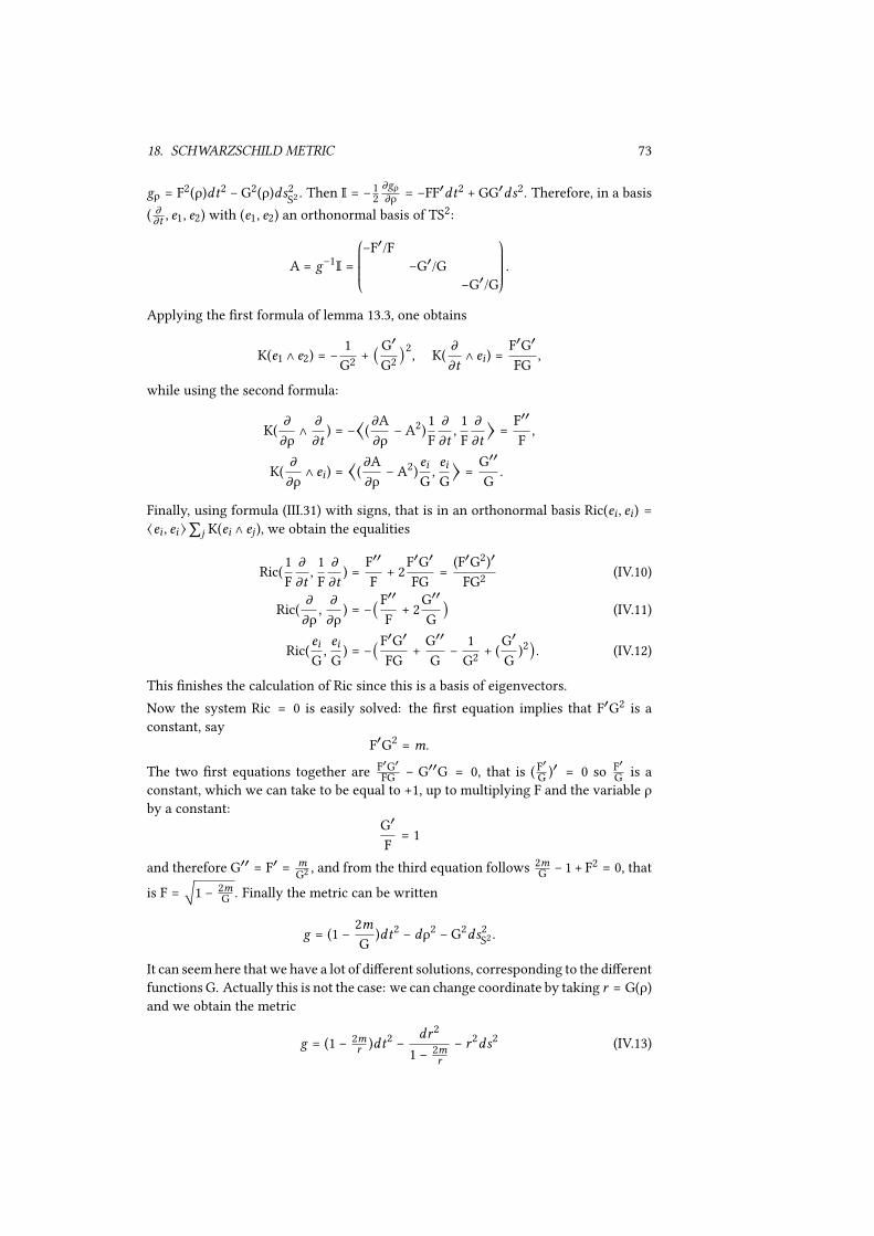
18. SCHWARZSCHILD METRIC 73
gρ = F2(ρ)dt
2− G
2(ρ)ds
2
S2. Then I = −
1
2
)gρ
)ρ= −FF
′dt2+ GG
′ds2. Therefore, in a basis
()
)t, e1, e2) with (e1, e2) an orthonormal basis of TS2:
A = g−1I =
⎛
⎜
⎜
⎝
−F′/F
−G′/G
−G′/G
⎞
⎟
⎟
⎠
.
Applying the �rst formula of lemma 13.3, one obtains
K(e1 ∧ e2) = −
1
G2+ (
G′
G2)
2
, K(
)
)t
∧ ei) =
F′G′
FG
,
while using the second formula:
K(
)
)ρ
∧
)
)t
) = −⟨(
)A
)ρ
− A2)
1
F
)
)t
,
1
F
)
)t⟩ =
F′′
F
,
K(
)
)ρ
∧ ei) = ⟨(
)A
)ρ
− A2)
ei
G
,
ei
G⟩ =
G′′
G
.
Finally, using formula (III.31) with signs, that is in an orthonormal basis Ric(ei , ei) =⟨ei , ei⟩∑j
K(ei ∧ ej ), we obtain the equalities
Ric(
1
F
)
)t
,
1
F
)
)t
) =
F′′
F
+ 2
F′G′
FG
=
(F′G2)′
FG2
(IV.10)
Ric(
)
)ρ
,
)
)ρ
) = −(
F′′
F
+ 2
G′′
G) (IV.11)
Ric(
ei
G
,
ei
G
) = −(
F′G′
FG
+
G′′
G
−
1
G2+ (
G′
G
)2
). (IV.12)
This �nishes the calculation of Ric since this is a basis of eigenvectors.Now the system Ric = 0 is easily solved: the �rst equation implies that F′G2 is aconstant, say
F′G2= m.
The two �rst equations together are F′G′
FG− G
′′G = 0, that is ( F′
G)′= 0 so F
′
Gis a
constant, which we can take to be equal to +1, up to multiplying F and the variable ρby a constant:
G′
F
= 1
and therefore G′′ = F′ = m
G2, and from the third equation follows 2m
G− 1 + F
2= 0, that
is F =√
1 −2m
G. Finally the metric can be written
g = (1 −
2m
G
)dt2− dρ
2− G
2ds2
S2 .
It can seem here that we have a lot of di�erent solutions, corresponding to the di�erentfunctionsG. Actually this is not the case: we can change coordinate by taking r = G(ρ)and we obtain the metric
g = (1 −2m
r)dt
2−
dr2
1 −2m
r
− r2ds2 (IV.13)

74 CHAPTER IV. EINSTEIN EQUATION
which depends only on one parameter m > 0. This is the Schwarzschild metric.Remark that when r → ∞ then g ∼ dt
2−dr
2− r
2ds2, so at large distance the Schwar-
zschild metric is asymptotic to the �at Minkowski metric on ℝ1,3. The Schwarzschild
is a model for the gravitation �eld of one central star, and a = 2m is called Schwarz-schild gravitation radius. For example, a = 3 km for the sun and a = 0, 44 cm for theearth.
18.c Null geodesics
Here we will show that the light is deviated by the gravitation �eld—one of the �rstcon�rmations of general relativity. In general relativity, the light propagates alongnull geodesics, that is along geodesics c such that ⟨c, c⟩ = 0. So we have to calculatethe geodesics. Certainly, we can restrict to calculate the geodesics lying inside totallygeodesic hypersurfaces of the form ℝ × I × S
1, where S1 ⊂ S2 is a great circle, on whichwe take an angular coordinate φ.We have Killing �elds )
)t, )
)φ, leading by lemma 9.8 to �rst integrals
ε = ⟨
)
)t
, c⟩ = (1 −
2m
r
)t ,
μ = −⟨
)
)φ
, c⟩ = r2φ.
Moreover for a light geodesic we have
(1 −2m
r)t2−
1
1 −2m
r
r2− r
2φ2= 0.
Replacing t and φ in this equation by their values in terms of ε and μ, one obtains
r2= ε
2−
1 −2m
r
r2
μ2.
Since r2 > 0, one must have
1 −2m
r
r2
6ε2
μ2.
The maximum value of the LHS is 1
27m2
at r = 3m. Then there are three cases:
1. ε2
μ2=
1
27m2, then r = 3m, the light ray remains inside the ‘photonic sphere’
r = 3m;
2. ε2
μ2<
1
27m2, then the geodesic remains outside or inside the photonic sphere;
3. ε2
μ2>
1
27m2, then r
2> 0 so r is monotone and the ray goes to the star or comes
from the star.
The deviation of light rays we are interested in is the second case.
star

18. SCHWARZSCHILD METRIC 75
We de�ne φc = φ(+∞) − φ(−∞). For a straight line, φc = π. We want to prove thatthere is a deviation, that is φc > π. One has dr
dφ=
r
φ=
r r2
μ, and
(
dr
dφ)
2
=
r4
μ2(ε2−
1 −2m
r
r2
μ2
)
=
m2
v2μ2(ε2m2
v2− (1 − 2v)μ
2
) with v =
m
r
.
It follows that
(
dv
dφ)
2
=
m2ε2
μ2
− v2+ 2v
3.
The variable v goes from 0 to a maximum value at, say, v0, such that v0 − 2v30 = m2ε2
μ2
,and then decreases back to 0; we can rewrite
(
dv
dφ)
2
= v2
0− 2v
3
0− v
2+ 2v
3,
and
φc = 2 ∫
v0
0
dφ
dv
dv = 2∫
v0
0
dv
√
v2
0− v
2
√
1 − 2v3
0−v
3
v2
0−v
2
> 2∫
v0
0
dv
√
v2
0− v
2(1 +
v3
0− v
3
v2
0− v
2) = π + 4v0.
This indeed proves that φc > π, so there is a deviation.For other applications of the Schwarzschild metric to general relativity, see for ex-ample the book [Bes87].

76 CHAPTER IV. EINSTEIN EQUATION

Chapter V
Some exercises
Complex projective space
Let us see the unit sphere S2n+1 ⊂ ℂn+1 equipped with the standard Hermitian product
⟨z, t⟩ = ∑ ziti . We de�ne a vector �eld T and a 1-form η on S2n+1 by: for any point
z ∈ S2n+1, one takes Tz = iz ∈ TzS
2n+1 and ηz(V) = ⟨T,V⟩ for any V ∈ TzS2n+1 (why
is this real ?).1° What is the �ow of the vector �eld T ? Prove that LTη = ιTdη = 0.2° Let p ∶ S2n+1 → ℂP
n be the natural projection. Prove that there is a unique 2-formΩ on ℂP
n such that dη = p∗Ω. Prove that Ω is symplectic, that is Ω is closed and
nondegenerate, cf. example 6.8, 3°. The form Ω is known as the Fubiny-Study form.3°Deduce thatΩk de�nes a nonzero cohomology class inH2k (ℂPn) for k 6 n. Actuallyone can show that this gives the whole cohomology, b
2k(ℂP
n) = 1 for k 6 n and
b2k+1
(ℂPn) = 0.
Isotopies
1° Let M be a manifold and (ψt )06t61 denote a smooth one-parameter family of dif-feomorphisms ((t, x)↦ ψt (x) is smooth). Prove that for any form α, one has d
dtψ∗
tα =
ψ∗
tLXt
α, where Xt is the time dependent vector �eld de�ned by Xt =dψt
dt◦ψ−1
t. Prove
that if α is closed, then
ψ∗
1α − ψ
∗
0α = d
(∫
1
0
ψ∗
t(ιXt
α)dt).
2° Prove the Poincaré lemma: any closed form of positive degree is locally exact. Hint:use 1° on a small ball of ℝn , with ψt (x) = tx and check that the apparent problem att = 0 is irrelevant.3° Prove the Hairy Ball theorem: there is no nonvanishing vector �eld on the sphereS2n . Hint: if such a vector �eld X existed, you could associate to any point x ∈ S2n the
point ψt (x) obtained by rotating x of an angle πt in the plane containing x and X(x);deduce that the standard volume form of S2n would be preserved by the antipodal
77

78 CHAPTER V. SOME EXERCISES
map. (Observe the previous exercise yields a nonvanishing vector �eld on the sphereS2n+1).
4° Prove the symplectic Darboux theorem: any symplectic form is locally isomorphicto the standard symplectic form
Ω0 =
n
∑
1
dxi∧ dx
i+n
on ℝ2n , namely Ω = ψ
∗Ω0 for some local di�eomorphism ψ. To prove this, you may
work in coordinates, on a small ball around 0 in ℝ2n , assume Ω and Ω0 coincide at
the origin and consider Ωt = tΩ + (1 − t)Ω0. The trick (known as Moser’s trick)consists in �nding a family of di�eomorphisms ψt such that ψ0 is the identity andψ∗
tΩt is constant in time, so that ψ1 will do the job. In order to build this family of
di�eomorphisms, you will �rst �nd the vector �elds Xt by computing the derivativeof ψ∗
tΩt and then integrate the time-dependent ordinary di�erential equation dψt
dt=
Xt ◦ψt .5° A distribution D of rank 2n on a manifold M2n+1 is called a contact distributionif it can be written locally as D = ker α some one-form α such that α ∧ (dα)n does notvanish; it is equivalent to require that the restriction of dα on D is non-degenerate.Prove the contact Darboux theorem: any contact distribution D on M2n+1 is locallyisomorphic to the standard contact structure on ℝ
2n+1, given by the kernel of
α0 = dx2n+1
−
n
∑
1
xidx
i+n.
Hint: Moser’s trick.
Gauss map
Let Σ be a connected compact surface embedded in ℝ3, with sectional curvature K > 0.
We do not suppose Σ orientable.1° Prove that the second fundamental form of Σ is de�nite positive or de�nite negativeat every point.2° For every x ∈ Σ we denote π the orthogonal projection ℝ
3→ (TxΣ)
⟂. Prove thatthe vector νx = − π(∇XX)
|π(∇XX)|does not depend on the non zero vector X ∈ TxΣ. Prove that
Σ is orientable.3° The application Γ ∶ Σ → S
2, given by Γ(x) = νx ∈ ℝ3, is called the Gauss map.
Prove that Γ is a di�eomorphism. Calculate Γ in case Σ = S2.4° Prove that Γ∗ volS2 = K volΣ (how general is this formula ?) Deduce in that case aproof of the Gauss-Bonnet formula,
1
2π∫Σ
KvolΣ= 2.
Umbilic submanifolds
1° Let Nn−1 be a submanifold of (Mn, g), oriented by the normal n, with second fun-
damental form I. Prove that, for all vectors X, Y and Z of N one has
⟨RM
X,YZ, n⟩ = ∇XI(Y,Z) − ∇YI(X,Z). (V.1)

79
(The RHS is (d∇I)(X,Y,Z) if one considers I as a TN-valued 1-form on N, and thisformula is the Gauss-Codazzi equation, see also remark 18.3.)2° The submanifold N is said totally umbilic if for every x ∈ N the second funda-mental form is a multiple of the metric: I = λ(x)g. If N is a totally umbilic subman-ifold of the �at ℝn , show that λ is a constant function. Deduce that the applicationϕ ∶ N → S
n−1 given by ϕ(x) = nx
λis a local isometry, and that N is a sphere (or an
open set of a sphere).3° Find all submanifolds N ⊂ ℝ
n with constant positive sectional curvature.
Submanifolds of the hyperbolic space
We choose coordinates in ℝ1,n such that the quadratic form is
ℎ(x, x) = 2x0x1− (x
2)2−⋯ − (x
n)2.
The hyperbolic space is the submanifold Hn= {ℎ(x, x) = 1, x
0> 0} with the induced
metric g = −ℎ.1° Choose on H
n coordinates (y1,… , yn) ∈ ℝ
∗
+× ℝ
n−1 by taking (x1= 1/y
1, x2=
y2/y1,… , x
n= y
n/y1). Prove that
g =
(dy1)2+ (dy
2)2+⋯ + (dy
n)2
(y1)2
(half-space model).2° Prove that for λ > 0 the homothety
(y1,… , y
n)→ (λy
1,… , λy
n)
and the inversion(y1,… , y
n)→
(y1,… , y
n)
(y1)2+⋯ + (y
n)2
are isometries of Hn .Prove that the intersection with H
n= {y
1> 0} of a sphere of ℝn centered on the
hyperplace {y1 = 0} is totally geodesic.3° If g2 and g1 are Riemannian metrics on a manifold Mn such that g2 = e
2fg1, where
f is a function, prove that their Levi-Civita connections satisfy
g1(∇g2
XY,Z) = g1(∇
g1
XY,Z) + df (X)g1(Y,Z) + df (Y)g1(X,Z) − g1(X,Y)df (Z).
Using the previous exercise, deduce that a submanifold Nn−1⊂ M is totally umbilic
for g1 if and only if it is totally umbilic for g2. Deduce all totally umbilic submanifoldsof Hn in the half-space model.
Toral black hole Einstein metrics
LetM = I×S1×T
n−2 the product of an interval I ofℝ, a circle S1 and a (n−2)-dimensionaltorus Tn−2.

80 CHAPTER V. SOME EXERCISES
1° Find all metrics g on M, satisfying the Einstein equation
Ric(g) = −(n − 1)g,
of the form g = ϕ(r)dr2+ ψ(r)dθ
2+ r
2gT, where r and θ are coordinates on I and S1,
gT is a �at metric on the torus T, and ϕ and ψ are functions of r only.Hint: �rst, look for a metric of the form dρ
2+ F
2(ρ)dθ
2+ G
2(ρ)gT.
2° These metrics are de�ned for an interval of the form I = (r+, +∞). Which metricdo we get when r+ = 0 ? prove that it is complete, with constant sectional curvatureequal to −1 (real hyperbolic cusp).3° Prove that in some cases, one can add in r = r+ a torus Tn−2, so that the metricextends to a complete smooth Einstein metric on M = M ∪ T
n−2.

Bibliography
[Bes87] Arthur L. Besse. Einstein manifolds. Springer-Verlag, Berlin, 1987.
[BGV04] Nicole Berline, Ezra Getzler, and Michèle Vergne. Heat kernels and Dirac op-erators. Grundlehren Text Editions. Springer-Verlag, Berlin, 2004. Correctedreprint of the 1992 original.
[GHL04] Sylvestre Gallot, Dominique Hulin, and Jacques Lafontaine. Riemanniangeometry. Universitext. Springer-Verlag, Berlin, third edition, 2004.
[Kob95] Shoshichi Kobayashi. Transformation groups in di�erential geometry. Clas-sics in Mathematics. Springer-Verlag, Berlin, 1995. Reprint of the 1972 edi-tion.
[Lee13] John M. Lee. Introduction to smooth manifolds, volume 218 of Graduate Textsin Mathematics. New York, NY: Springer, 2nd revised edition, 2013.
81

Index
atlas, 12
Bianchi identity, 54, 70boundary, 33bracket, 22
chart, 9Chern classes, 67Christo�el symbols, 38closed manifold, 33complete Riemannian manifold, 48complete vector �eld, 23complex manifold, 13complex projective space, 14conjugacy radius, 61conjugate point, 63connection, 38connection 1-form, 38contact distribution, 78cotangent bundle, 19covariant derivative, 38curvature, 53, 54curvature operator, 55
derivation, 21di�eomorphism, 15di�erential Bianchi identity, 65, 70di�erential form, 27dimension, 12distribution, 24
Einstein metric, 71embedding, 12energy, 44equivalent atlases, 12equivalent paths, 16Euler form, 68Euler number, 68exterior derivative, 29
�rst integral, 45�at, 53�ow, 23Fubiny-Study form, 77
Gauss map, 78geodesic, 44
homogeneous coordinates, 14horizontal distribution, 51horizontal lift, 51
immersion, 11injectivity radius, 46integrable, 25integral curves, 25integral submanifold, 25interior product, 30involutive, 25isometry, 37
Killing �eld, 45
leaf, 25length, 43Levi-Civita connection, 42Lie derivative, 20, 23, 29local coordinates, 15local trivializations, 19
manifold, 12manifold with boundary, 33mean curvature, 59metric, 40metric connection, 41minimal surfaces, 59minimizing paths, 43Moser’s trick, 78
normal coordinates, 46
82

INDEX 83
odd derivation, 28orientable, 31orientation, 31
parallel transport, 42partition of unity, 31Pfa�an, 67principal curvatures, 59pseudo-Riemannian metrics, 35pull-back, 23, 28
real projective space, 14Ricci tensor, 62Riemannian metric, 35
scalar curvature, 69second fundamental form, 56sectional curvature, 55smooth map between two manifolds, 15smooth section, 19submanifold, 9, 15submersion, 10symplectic form, 32
tangent map, 18tangent space, 10, 16tangent vector, 10, 16tensorial, 28topological manifold, 13torsion, 42torsion-free connection, 42totally geodesic submanifold, 71totally umbilic, 79transgression formulas, 66transition functions, 12
unitary connection, 41
vector bundle, 19vector �elds, 20vertical space, 52volume form, 31, 36
Weingarten endomorphism, 57