introduction to dsp - technical · web viewintroduction to dsp a signal is any variable that...
TRANSCRIPT
Rajalakshmi Engineering College Thandalam
Prepared by JVijayaraghavan Asst ProfECE
DIGITAL SIGNAL PROCESSING III YEAR ECE B
Introduction to DSP
A signal is any variable that carries information Examples of the types of signals of interest are Speech (telephony radio everyday communication) Biomedical signals (EEG brain signals) Sound and music Video and image_ Radar signals (range and bearing)
Digital signal processing (DSP) is concerned with the digital representation of signals and the use of digital processors to analyse modify or extract information from signals Many signals in DSP are derived from analogue signals which have been sampled at regular intervals and converted into digital form The key advantages of DSP over analogue processing are Guaranteed accuracy (determined by the number of bits used) Perfect reproducibility No drift in performance due to temperature or age Takes advantage of advances in semiconductor technology Greater exibility (can be reprogrammed without modifying hardware) Superior performance (linear phase response possible and_ltering algorithms can be made adaptive) Sometimes information may already be in digital form There are however (still) some disadvantages Speed and cost (DSP design and hardware may be expensive especially with high bandwidth signals) Finite word length problems (limited number of bits may cause degradation)
Application areas of DSP are considerable _ Image processing (pattern recognition robotic vision image enhancement facsimile satellite weather map animation) Instrumentation and control (spectrum analysis position and rate control noise reduction data compression) _ Speech and audio (speech recognition speech synthesis text to Speech digital audio equalisation) Military (secure communication radar processing sonar processing missile guidance) Telecommunications (echo cancellation adaptive equalisation spread spectrum video conferencing data communication) Biomedical (patient monitoring scanners EEG brain mappers ECG analysis X-ray storage and enhancement)
UNIT I
Discrete-time signals
A discrete-time signal is represented as a sequence of numbers
Here n is an integer and x[n] is the nth sample in the sequence Discrete-time signals are often obtained by sampling continuous-time signals In this case the nth sample of the sequence is equal to the value of the analogue signal xa(t) at time t = nT
The sampling period is then equal to T and the sampling frequency is fs = 1=T x[1]
For this reason although x[n] is strictly the nth number in the sequence we often refer to it as the nth sample We also often refer to the sequence x[n] when we mean the entire sequence Discrete-time signals are often depicted graphically as follows
(This can be plotted using the MATLAB function stem) The value x[n] is unde_ned for no integer values of n Sequences can be manipulated in several ways The sum and product of two sequences x[n] and y[n] are de_ned as the sample-by-sample sum and product respectively Multiplication of x[n] by a is de_ned as the multiplication of each sample value by a A sequence y[n] is a delayed or shifted version of x[n] if
with n0 an integerThe unit sample sequence
is defined as
This sequence is often referred to as a discrete-time impulse or just impulse It plays the same role for discrete-time signals as the Dirac delta function does for continuous-time signals However there are no mathematical complications in its definitionAn important aspect of the impulse sequence is that an arbitrary sequence can be represented as a sum of scaled delayed impulses Forexample the
Sequence can be represented as
In general any sequence can be expressed as
The unit step sequence is defined as
The unit step is related to the impulse by Alternatively this can be expressed as
Conversely the unit sample sequence can be expressed as the _rst backward difference of the unit step sequence
Exponential sequences are important for analyzing and representing discrete-time systems The general form is
If A and _ are real numbers then the sequence is real If 0 lt _ lt 1 and A is positive then the sequence values are positive and decrease with increasing n
For 10485761 lt _ lt 0 the sequence alternates in sign but decreases in magnitude For j_j gt 1 the sequence grows in magnitude as n increases A sinusoidal sequence
has the form
The frequency of this complex sinusoid is0 and is measured in radians per sample The phase of the signal is The index n is always an integer This leads to some importantDifferences between the properties of discrete-time and continuous-time complex exponentials Consider the complex exponential with frequency
Thus the sequence for the complex exponential with frequency is exactly the same as that for the complex exponential with frequency more generally complex exponential sequences with frequencies where r is an integer are indistinguishableFrom one another Similarly for sinusoidal sequences
In the continuous-time case sinusoidal and complex exponential sequences are always periodic Discrete-time sequences are periodic (with period N) if x[n] = x[n + N] for all n
Thus the discrete-time sinusoid is only periodic if
which requires that
The same condition is required for the complex exponential
Sequence to be periodic The two factors just described can be combined to reach the conclusion that there are only N distinguishable frequencies for which theCorresponding sequences are periodic with period N One such set is
Discrete-time systemsA discrete-time system is de_ned as a transformation or mapping operator that maps an input signal x[n] to an output signal y[n] This can be denoted as
Example Ideal delay
Memoryless systemsA system is memory less if the output y[n] depends only on x[n] at the
Same n For example y[n] = (x[n]) 2 is memory less but the ideal delay
Linear systemsA system is linear if the principle of superposition applies Thus if y1[n]is the response of the system to the input x1[n] and y2[n] the responseto x2[n] then linearity implies
Additivity
Scaling
These properties combine to form the general principle of superposition
In all cases a and b are arbitrary constants This property generalises to many inputs so the response of a linearsystem toTime-invariant systems
A system is time invariant if times shift or delay of the input sequenceCauses a corresponding shift in the output sequence That is if y[n] is the response to x[n] then y[n -n0] is the response to x[n -n0]For example the accumulator system
is time invariant but the compressor system
for M a positive integer (which selects every Mth sample from a sequence) is notCausalityA system is causal if the output at n depends only on the input at nand earlier inputs For example the backward difference system
is causal but the forward difference system
is notStability
A system is stable if every bounded input sequence produces a boundedoutput sequence
x[n]is an example of an unbounded system since its response to the unit
This has no _nite upper bound Linear time-invariant systemsIf the linearity property is combined with the representation of a general sequence as a linear combination of delayed impulses then it follows that a linear time-invariant (LTI) system can be completely characterized by its impulse response Suppose hk[n] is the response of a linear system to the impulse h[n -k]at n = k Since
If the system is additionally time invariant then the response to _[n -k] is h[n -k] The previous equation then becomes
This expression is called the convolution sum Therefore a LTI system has the property that given h[n] we can _nd y[n] for any input x[n] Alternatively y[n] is the convolution
of x[n] with h[n] denoted as follows The previous derivation suggests the interpretation that the input sample at n = k
represented by is transformed by the system into an output sequence
For each k these sequences are superimposed to yield the overall output sequence A slightly different interpretation however leads to a convenient computational form the nth value of the output namely y[n] is obtained by multiplying the input sequence (expressed as a function of k) by the sequence with values h[n-k] and then summing all the values of the products x[k]h[n-k] The key to this method is in understanding how to form the sequence h[n -k] for all values of n of interest To this end note that h[n -k] = h[- (k -n)] The sequence h[-k] is seen to be equivalent to the sequence h[k] rejected around the origin
Since the sequences are non-overlapping for all negative n the output must be zero y[n] = 0 n lt 0
The Discrete Fourier TransformThe discrete-time Fourier transform (DTFT) of a sequence is a continuous function of and repeats with period 2_ In practice we usually want to obtain the Fourier components using digital computation and can only evaluate them for a discrete set of frequencies The discrete Fourier transform (DFT) provides a means for achieving this The DFT is itself a sequence and it corresponds roughly to samples equally spaced in frequency of the Fourier transform of the signal The discrete Fourier transform of a length N signal x[n] n = 0 1 N -1 is given by
An important property of the DFT is that it is cyclic with period N both in the discrete-time and discrete-frequency domains For example for any integer r
since Similarly it is easy to show that x[n + rN] = x[n] implying periodicity of the synthesis equation This is important | even though the DFT only depends on samples in the interval 0 to N -1 it is implicitly assumed that the signals repeat with period N in both the time and frequency domains To this end it is sometimes useful to de_ne the periodic extension of the signal x[n] to be To this end it is sometimes useful to de_ne the periodic extension of the signal x[n] to be x[n] = x[n mod N] = x[((n))N] Here n mod N and ((n))N are taken to mean n modulo N which has the value of the remainder after n is divided by N Alternatively if n is written in the form n = kN + l for 0 lt l lt N then n mod N = ((n))N = l
It is sometimes better to reason in terms of these periodic extensions when dealing with the DFT Specifically if X[k] is the DFT of x[n] then the inverse DFT of X[k] is ~x[n] The signals x[n] and ~x[n] are identical over the interval 0 to N 1048576 1 but may differ outside of this range Similar statements can be made regarding the transform Xf[k] Properties of the DFTMany of the properties of the DFT are analogous to those of the discrete-time Fourier transform with the notable exception that all shifts involved must be considered to be circular or modulo N Defining the DFT pairs and
Linear convolution of two finite-length sequences Consider a sequence x1[n] with length L points and x2[n] with length P points The linear convolution of the sequences
Therefore L + P 1048576 1 is the maximum length of x3[n] resulting from theLinear convolution The N-point circular convolution of x1[n] and x2[n] is
It is easy to see that the circular convolution product will be equal to the linear convolution product on the interval 0 to N 1048576 1 as long as we choose N - L + P +1 The process of augmenting a sequence with zeros to make it of a required length is called zero paddingFast Fourier transformsThe widespread application of the DFT to convolution and spectrum analysis is due to the existence of fast algorithms for its implementation The class of methods is referred to as fast Fourier transforms (FFTs) Consider a direct implementation of an 8-point DFT
If the factors have been calculated in advance (and perhaps stored in a lookup table) then the calculation of X[k] for each value of k requires 8 complex multiplications
and 7 complex additions The 8-point DFT therefore requires 8 8 multiplications and 8 7 additions For an N-point DFT these become N2 and N (N - 1) respectively If N = 1024 then approximately one million complex multiplications and one million complex additions are required The key to reducing the computational complexity lies in theObservation that the same values of x[n] are effectively calculated many times as the computation proceeds | particularly if the transform is long The conventional decomposition involves decimation-in-time where at each stage a N-point transform is decomposed into two N=2-point transforms That is X[k] can be written as X[k] =N
The original N-point DFT can therefore be expressed in terms of two N=2-point DFTsThe N=2-point transforms can again be decomposed and the process repeated until only 2-point transforms remain In general this requires log2N stages of decomposition Since each stage requires approximately N complex multiplications the complexity of the resulting algorithm is of the order of N log2 N The difference between N2 and N log2 N complex multiplications can become considerable for large values of N For example if N = 2048 then N2=(N log2 N) _ 200 There are numerous variations of FFT algorithms and all exploit the basic redundancy in the computation of the DFT In almost all cases anOf the shelf implementation of the FFT will be sufficient | there is seldom any reason to implement a FFT yourself
Some forms of digital filters are more appropriate than others when real-world effects are considered This article looks at the effects of finite word length and suggests that some implementation forms are less susceptible to the errors that finite word length effects introduce In articles about digital signal processing (DSP) and digital filter design one thing Ive noticed is that after an in-depth development of the filter design the implementation is often just given a passing nod References abound concerning digital filter design but surprisingly few deal with implementation The implementation of a digital filter can take many forms Some forms are more appropriate than others when various real-world effects are considered This article examines the effects of finite word length It suggests that certain implementation forms are less susceptible than others to the errors introduced by finite word length effects
UNIT III
Finite word length Most digital filter design techniques are really discrete time filter design
techniques Whats the difference Discrete time signal processing theory assumes discretization of the time axis only Digital signal processing is discretization on the time and amplitude axis The theory for discrete time signal processing is well developed and can be handled with deterministic linear models Digital signal processing on the other hand requires the use of stochastic and nonlinear models In discrete time signal processing the amplitude of the signal is assumed to be a continuous value-that is the amplitude can be any number accurate to infinite precision When a digital filter design is moved from theory to implementation it is typically implemented on a digital computer Implementation on a computer means quantization in time and amplitude-which is true digital signal processing Computers implement real values in a finite number of bits Even floating-point numbers in a computer are implemented with finite precision-a finite number of bits and a finite word length Floating-point numbers have finite precision but dynamic scaling afforded by the floating point reduces the effects of finite precision Digital filters often need to have real-time performance-that usually requires fixed-point integer arithmetic With fixed-point implementations there is one word size typically dictated by the machine architecture Most modern computers store numbers in twos complement form Any real number can be represented in twos complement form to infinite precision as in Equation 1
where bi is zero or one and Xm is scale factor If the series is truncated to B+1 bits where b0 is a sign bit there is an error between the desired number and the truncated number The series is truncated by replacing the infinity sign in the summation with B the number of bits in the fixed-point word The truncated series is no longer able to represent an arbitrary number-the series will have an error equal to the part of the series discarded The statistics of the error depend on how the last bit value is determined either by truncation or rounding Coefficient Quantization The design of a digital filter by whatever method will eventually lead to an equation that can be expressed in the form of Equation 2
with a set of numerator polynomial coefficients bi and denominator polynomial coefficients ai When the coefficients are stored in the computer they must be truncated to some finite precision The coefficients must be quantized to the bit length of the word size used in the digital implementation This truncation or quantization can lead to problems in the filter implementation The roots of the numerator polynomial are the zeroes of the system and the roots of the denominator polynomial are the poles of the system When the coefficients are quantized the effect is to constrain the allowable pole zero locations in the complex plane If the coefficients are quantized they will be forced to lie on a grid of points similar to those in Figure 1 If the grid points do not lie exactly
on the desired infinite precision pole and zero locations then there is an error in the implementation The greater the number of bits used in the implementation the finer the grid and the smaller the error So what are the implications of forcing the pole zero locations to quantized positions If the quantization is coarse enough the poles can be moved such that the performance of the filter is seriously degraded possibly even to the point of causing the filter to become unstable This condition will be demonstrated later Rounding Noise
When a signal is sampled or a calculation in the computer is performed the results must be placed in a register or memory location of fixed bit length Rounding the value to the required size introduces an error in the sampling or calculation equal to the value of the lost bits creating a nonlinear effect Typically rounding error is modeled as a normally distributed noise injected at the point of rounding This model is linear and allows the noise effects to be analyzed with linear theory something we can handle The noise due to rounding is assumed to have a mean value equal to zero and a variance given in Equation 3
For a derivation of this result see Discrete Time Signal Processing1 Truncating the value (rounding down) produces slightly different statistics Multiplying two B-bit variables results in a 2B-bit result This 2B-bit result must be rounded and stored into a B-bit length storage location This rounding occurs at every multiplication point
Scaling We dont often think about scaling when using floating-point calculations because the computer scales the values dynamically Scaling becomes an issue when using fixed-point arithmetic where calculations would cause over- or under flow In a filter with multiple stages or more than a few coefficients calculations can easily overflow the word length Scaling is required to prevent over- and under flow and if placed strategically can also help offset some of the effects of quantization
Signal Flow Graphs Signal flow graphs a variation on block diagrams give a slightly more compact notation A signal flow graph has nodes and branches The examples shown here will use a node as a summing junction and a branch as a gain All inputs into a node are summed while any signal through a branch is scaled by the gain along the branch If a branch contains a delay element its noted by a z yacute 1 branch gain Figure 2 is an example of the basic elements of a signal flow graph Equation 4 results from the signal flow graph in Figure 2
Finite Precision Effects in Digital Filters
Causal linear shift-invariant discrete time system difference equation
Z-Transform
where is the Z-Transform Transfer Function
and is the unit sample response
Where
Is the sinusoidal steady state magnitude frequency response
Is the sinusoidal steady state phase frequency response
is the Normalized frequency in radians
if
then
If the input is a sinusoidal signal of frequency then the output is a
sinusoidal signal of frequency (LINEAR SYSTEM)
If the input sinusoidal frequency has an amplitude of one and a phase of zero then the output is a sinusoidal (of the same frequency) with a magnitude
and phase
So by selecting and
can be determine in terms of the filter order and coefficients
(Filter Synthesis) If the linear constant coefficient difference equation is implemented directly
Magnitude Frequency Response
Magnitude Frequency Response (Pass band only)
However to implement this discrete time filter finite precision arithmetic (even if it is floating point) is used
This implementation is a DIGITAL FILTER There are two main effects which occur when finite precision arithmetic is used to implement a DIGITAL FILTER Multiplier coefficient quantization Signal quantization
1 Multiplier coefficient quantizationThe multiplier coefficient must be represented using a finite number of bits To do this the coefficient value is quantized For example a multiplier coefficient
might be implemented as
The multiplier coefficient value has been quantized to a six bit (finite precision) value The value of the filter coefficient which is actually implemented is 5264 or 08125 AS A RESULT THE TRANSFER FUNCTION CHANGES
The magnitude frequency response of the third order direct form filter (with the gain or scaling coefficient removed) is
2 Signal quantizationThe signals in a DIGITAL FILTER must also be represented by finite quantized binary values There are two main consequences of this A finite RANGE for signals (IE a maximum value) Limited RESOLUTION (the smallest value is the least significant bit) For n-bit twos complement fixed point numbers
If two numbers are added (or multiplied by and integer value) then the result can be larger than the most positive number or smaller than the most negative number When this happens an overflow has occurred If twos complement arithmetic is used then the
effect of overflow is to CHANGE the sign of the result and severe large amplitude nonlinearity is introduced For useful filters OVERFLOW cannot be allowed To prevent overflow the digital hardware must be capable of representing the largest number which can occur It may be necessary to make the filter internal word length larger than the inputoutput signal word length or reduce the input signal amplitude in order to accommodate signals inside the DIGITAL FILTER Due to the limited resolution of the digital signals used to implement the DIGITAL FILTER it is not possible to represent the result of all DIVISION operations exactly and thus the signals in the filter must be quantized
The nonlinear effects due to signal quantization can result in limit cycles - the filter output may oscillate when the input is zero or a constant In addition the filter may exhibit dead bands - where it does not respond to small changes in the input signal amplitude The effects of this signal quantization can be modeled by
where the error due to quantization (truncation of a twos complement number) is
By superposition the can determine the effect on the filter output due to each quantization source To determine the internal word length required to prevent overflow and the error at the output of the DIGITAL FILTER due to quantization find the GAIN from the input to every internal node Either increases the internal wordlengh so that overflow does not occur or reduce the amplitude of the input signal Find the GAIN from each quantization point to the output Since the maximum value of e(k) is known a bound on the largest error at the output due to signal quantization can be determined using Convolution Summation Convolution Summation (similar to Bounded-Input Bounded-Output stability requirements)
If
then
is known as the norm of the unit sample response It is a necessary and sufficient condition that this value be bounded (less than infinity) for the linear system to be Bounded-Input Bounded-Output Stable
The norm is one measure of the GAIN
Computing the norm for the third order direct form filter input node 3 output node 8L1 norm between (3 8) ( 17 points) 1267824L1 norm between (3 4) ( 15 points ) 3687712L1 norm between (3 5) ( 15 points ) 3685358L1 norm between (3 6) ( 15 points ) 3682329L1 norm between (3 7) ( 13 points ) 3663403
MAXIMUM = 3687712L1 norm between (4 8) ( 13 points ) 1265776L1 norm between (4 8) ( 13 points ) 1265776L1 norm between (4 8) ( 13 points ) 1265776L1 norm between (8 8) ( 2 points ) 1000000
SUM = 4797328
An alternate filter structure can be used to implement the same ideal transfer function
Third Order LDI Magnitude Response
Third Order LDI Magnitude Response (Pass band Detail)
Note that the effects of the same coefficient quantization as for the Direct Form filter (six bits) does not have the same effect on the transfer function This is because of the reduced sensitivity of this structure to the coefficients (A general property of integrator based ladder structures or wave digital filters which have a maximum power transfer characteristic)
LDI3 Multipliers s1 = 0394040030717361 s2 = 0659572897901019 s3 = 0650345952330870
Note that all coefficient values are less than unity and that only three multiplications are required There is no gain or scaling coefficient More adders are required than for the direct form structure
The norm values for the LDI filter are input node 1 output node 9L1 norm between (1 9) ( 13 points ) 1258256L1 norm between (1 3) ( 14 points ) 2323518L1 norm between (1 7) ( 14 points ) 0766841L1 norm between (1 6) ( 14 points ) 0994289
MAXIMUM = 2323518L1 norm between (10021 9) ( 16 points ) 3286393L1 norm between (10031 9) ( 17 points ) 3822733L1 norm between (10011 9) ( 17 points ) 3233201
SUM = 10342327Note that even though the ideal transfer functions are the same the effects of finite precision arithmetic are different To implement the direct form filter three additions and four multiplications are required Note that the placement of the gain or scaling coefficient will have a significant effect on the wordlenght or the error at the output due to quantization
Of course a finite-duration impulse response (FIR) filter could be used It will still have an error at the output due to signal quantization but this error is bounded by the number of multiplications A FIR filter cannot be unstable for bounded inputs and coefficients and piecewise linear phase is possible by using symmetric or anti-symmetric coefficients But as a rough rule an FIR filter order of 100 would be required to build a filter with the same selectivity as a fifth order recursive (Infinite Duration Impulse Response - IIR) filter Effects of finite word lengthQuantization and multiplication errorsMultiplication of 2 M-bit words will yield a 2M bit product which is or to an M bit word Truncated roundedSuppose that the 2M bit number represents an exact value then
Exact value x (2M bits) digitized value x (M bits) error e = x - xTruncationx is represented by (M -1) bits the remaining least significant bits of x being discarded
Quantization errorsQuantization is a nonlinearity which when introduced into a control loop can lead to orSteady state errorLimit cyclesStable limit cycles generally occur in control systems with lightly damped poles detailed nonlinear analysis or simulation may be required to quantify their effect methods of reducing the effects are- Larger word sizes- Cascade or parallel implementations- Slower sample ratesIntegrator OffsetConsider the approximate integral term
Practical features for digital controllersScalingAll microprocessors work with finite length words 8 16 32 or 64 bitsThe values of all input output and intermediate variables must lie within theRange of the chosen word length This is done by appropriate scaling of the variablesThe goal of scaling is to ensure that neither underflows nor overflows occur during arithmetic processingRange-checkingCheck that the output to the actuator is within its capability and saturatethe output value if it is not It is often the case that the physical causes of saturation are variable with temperature aging and operating conditionsRoll-overOverflow into the sign bit in output data may cause a DAC to switch from a high positiveValue to a high negative value this can have very serious consequences for the actuator and Plant Scaling for fixed point arithmeticScaling can be implemented by shiftingbinary values left or right to preserve satisfactory dynamic range and signal to quantization noise ratio Scale so that m is the smallest positive integer that satisfies the condition
UNIT IIFilter design1 Design considerations a framework
The design of a digital filter involves five steps_ Specification The characteristics of the filter often have to be specified in the frequency domain For example for frequency selective filters (low pass high pass band pass etc) the specification usually involves tolerance limits as shown above Coefficient calculation Approximation methods have to be used to calculate the values h[k] for a FIR implementation or ak bk for an IIR implementation Equivalently this involves finding a filter which has H (z) satisfying the requirements Realization This involves converting H(z) into a suitable filter structure Block or few diagrams are often used to depict filter structures and show the computational procedure for implementingthe digital filter Analysis of finite word length effects In practice one should check that the quantization used in the implementation does not degrade the performance of the filter to a point where it is unusable Implementation The filter is implemented in software or hardware The criteria for selecting the implementation method involve issues such as real-time performance complexity processing requirements and availability of equipment Finite impulse response (FIR) filters design A FIR _lter is characterized by the equations
The following are useful properties of FIR filters They are always stable | the system function contains no poles This is
particularly useful for adaptive filters They can have an exactly linear phase response The result is no frequency dispersion which is good for pulse and data transmission _ Finite length register effects are simpler to analyse and of less consequence than for IIR filters They are very simple to implement and all DSP processors have architectures that are suited to FIR filtering
The center of symmetry is indicated by the dotted line The process of linear-phase filter design involves choosing the a[n] values to obtain a filter with a desired frequency response This is not always possible however | the frequency response for a type II filter for example has the property that it is always zero for = _ and is therefore not appropriate for a high pass filter Similarly filters of type 3 and 4 introduce a 90_ phase shift and have a frequency response that is always zero at = 0 which makes them unsuitable for as lowpass filters Additionally the type 3 response is always zero at = _
making it unsuitable as a high pass filter The type I filter is the most versatile of the four Linear phase filters can be thought of in a different way Recall that a linear phase characteristic simply corresponds to a time shift or delay Consider now a real FIR _lter with an impulse response that satisfies the even symmetry condition h[n] = h[1048576n] H(ej) Increasing the length N of h[n] reduces the main lobe width and hence the transition width of the overall response The side lobes of W (ej) affect the pass band and stop band tolerance of H (ej) This can be controlled by changing the shape of the window Changing N does not affect the side lobe behavior Some commonly used windows for filter design are
All windows trade of a reduction in side lobe level against an increase in main lobe width This is demonstrated below in a plot of the frequency response of each of the window
Some important window characteristics are compared in the following
The Kaiser window has a number of parameters that can be used to explicitly tune the characteristics In practice the window shape is chosen first based on pass band and stop band tolerance requirements The window size is then determined based on transition width requirements To determine hd[n] from Hd(ej) one can sample Hd(ej) closely and use a large inverse DFT
Frequency sampling method for FIR filter designIn this design method the desired frequency response Hd(ej) is sampled at equally-spaced points and the result is inverse discrete Fourier transformed Specifically letting
The resulting filter will have a frequency response that is exactly the same as the original response at the sampling instants Note that it is also necessary to specify the phase of the
desired response Hd(ej) and it is usually chosen to be a linear function of frequency to ensure a linear phase filter Additionally if a filter with real-valued coefficients is required then additional constraints have to be enforced The actual frequency response H(ej) of the _lter h[n] still has to be determined The z-transform of the impulse response is
This expression can be used to _nd the actual frequency response of the _lter obtained which can be compared with the desired response The method described only guarantees correct frequency response values at the points that were sampled This sometimes leads to excessive ripple at intermediate points
Infinite impulse response (IIR) filter designAn IIR _lter has nonzero values of the impulse response for all values of n even as n 1 To implement such a _lter using a FIR structure therefore requires an infinite number of calculations However in many cases IIR filters can be realized using LCCDEs and computed recursivelyExampleA _lter with the infinite impulse response h[n] = (1=2)nu[n] has z-transform
Therefore y[n] = 1=2y [n +1] + x[n] and y[n] is easy to calculate IIR filter structures can therefore be far more computationally efficient than FIR filters particularly for long impulse responses FIR filters are stable for h[n] bounded and can be made to have a linear phase response IIR filters on the other hand are stable if the poles are inside the unit circle and have a phase response that is difficult to specify The general approach taken is to specify the magnitude response and regard the phase as acceptable This is aDisadvantage of IIR filters IIR filter design is discussed in most DSP texts
UNIT VDSP Processor- Introduction
DSP processors are microprocessors designed to perform digital signal processingmdashthe mathematical manipulation of digitally represented signals Digital signal processing is one of the core technologies in rapidly growing application areas such as wireless communications audio and video processing and industrial control Along with the rising popularity of DSP applications the variety of DSP-capable processors has expanded greatly since the introduction of the first commercially successful DSP chips in the early 1980s Market research firm Forward Concepts projects that sales of DSP processors will total US $62 billion in 2000 a growth of 40 percent over 1999 With semiconductor manufacturers vying for bigger shares of this booming market designersrsquo choices will broaden even further in the next few years Todayrsquos DSP processors (or ldquoDSPsrdquo) are sophisticated devices with impressive capabilities In this paper we introduce the features common to modern commercial DSP processors explain some of the important differences among these devices and focus on features that a system designer should examine to find the processor that best fits his or her application
What is a DSP ProcessorMost DSP processors share some common basic features designed to support
high-performance repetitive numerically intensive tasks The most often cited of these features are the ability to perform one or more multiply-accumulate operations (often called ldquoMACsrdquo) in a single instruction cycle The multiply-accumulate operation is useful in DSP algorithms that involve computing a vector dot product such as digital filters correlation and Fourier transforms To achieve a single-cycle MAC DSP processors integrate multiply-accumulate hardware into the main data path of the processor as shown in Figure 1 Some recent DSP processors provide two or more multiply-accumulate units allowing multiply-accumulate operations to be performed in parallel In addition to allow a series of multiply-accumulate operations to proceed without the possibility of arithmetic overflow (the generation of numbers greater than the maximum value the processorrsquos accumulator can hold) DSP processors generally provide extra ldquoguardrdquo bits in the accumulator For example the Motorola DSP processor family examined in Figure 1 offers eight guard bits A second feature shared by DSP processors is the ability to complete several accesses to memory in a single instruction cycle This allows the processor to fetch an instruction while simultaneously fetching operands andor storing the result of a previous instruction to memory For example in calculating the vector dot product for an FIR filter most DSP processors are able to perform a MAC while simultaneously loading the data sample and coefficient for the next MAC Such single cycle multiple memory accesses are often subject to many restrictions Typically all but one of the memory locations accessed must reside on-chip and multiple memory accesses can only take place with certain instructions
To support simultaneous access of multiple memory locations DSP processors provide multiple onchip buses multi-ported on-chip memories and in some case multiple independent memory banks A third feature often used to speed arithmetic processing on DSP processors is one or more dedicated address generation units Once the appropriate addressing registers have been configured the address generation unit Operates in the
background (ie without using the main data path of the processor) forming the address
Required for operand accesses in parallel with the execution of arithmetic instructions In contrast general-purpose processors often require extra cycles to generate the addresses needed to load operands DSP processor address generation units typically support a selection of addressing modes tailored to DSP applications The most common of these is register-indirect addressing with post-increment which is used in situations where a repetitive computation is performed on data stored sequentially in memory Modulo addressing is often supported to simplify the use of circular buffers Some processors also support bit-reversed addressing which increases the speed of certain fast Fourier transform (FFT) algorithms Because many DSP algorithms involve performing repetitive computations most DSP processors provide special support for efficient looping Often a special loop or repeat instruction is provided which allows the programmer to implement a for-next loop without expending any instruction cycles for updating and testing the loop counter or branching back to the top of the loop Finally to allow low-cost high-performance input and output most DSP processors incorporate one or more serial or parallel IO interfaces and specialized IO handling mechanisms such as low-overhead interrupts and direct memory access (DMA) to allow data transfers to proceed with little
or no intervention from the rest of the processor The rising popularity of DSP functions such as speech coding and audio processing has led designers to consider implementing DSP on general-purpose processors such as desktop CPUs and microcontrollers Nearly all general-purpose processor manufacturers have responded by adding signal processing capabilities to their chips Examples include the MMX and SSE instruction set extensions to the Intel Pentium line and the extensive DSP-oriented retrofit of Hitachirsquos SH-2 microcontroller to form the SH-DSP In some cases system designers may prefer to use a general-purpose processor rather than a DSP processor Although general-purpose processor architectures often require several instructions to perform operations that can be performed with just one DSP processor instruction some general-purpose processors run at extremely fast clock speeds If the designer needs to perform non- DSP processing and then using a general-purpose processor for both DSP and non-DSP processing could reduce the system parts count and lower costs versus using a separate DSP processor and general-purpose microprocessor Furthermore some popular general-purpose processors feature a tremendous selection of application development tools On the other hand because general-purpose processor architectures generally lack features that simplify DSP programming software development is sometimes more tedious than on DSP processors and can result in awkward code thatrsquos difficult to maintain Moreover if general-purpose processors are used only for signal processing they are rarely cost-effective compared to DSP chips designed specifically for the task Thus at least in the short run we believe that system designers will continue to use traditional DSP processors for the majority of DSP intensive applications We focus on DSP processors in this paper
ApplicationsDSP processors find use in an extremely diverse array of applications from radar
systems to consumer electronics Naturally no one processor can meet the needs of all or even most applications Therefore the first task for the designer selecting a DSP processor is to weigh the relative importance of performance cost integration ease of development power consumption and other factors for the application at hand Here wersquoll briefly touch on the needs of just a few classes of DSP applications In terms of dollar volume the biggest applications for digital signal processors are inexpensive high-volume embedded systems such as cellular telephones disk drives (where DSPs are used for servo control) and portable digital audio players In these applications cost and integration are paramount For portable battery-powered products power consumption is also critical Ease of development is usually less important even though these applications typically involve the development of custom software to run on the DSP and custom hardware surrounding the DSP the huge manufacturing volumes justify expending extra development effort
A second important class of applications involves processing large volumes of data with complex algorithms for specialized needs Examples include sonar and seismic exploration where production volumes are lower algorithms more demanding and product designs larger and more complex As a result designers favor processors with maximum performance good ease of use and support for multiprocessor configurations In some cases rather than designing their own hardware and software from scratch designers assemble such systems using off-the-shelf development boards and ease their
software development tasks by using existing function libraries as the basis of their application software
Choosing the Right DSP ProcessorAs illustrated in the preceding section the right DSP processor for a job depends heavily on the application One processor may perform well for some applications but be a poor choice for others With this in mind one can consider a number of features that vary from one DSP to another in selecting a processor These features are discussed belowArithmetic Format
One of the most fundamental characteristics of a programmable digital signal processor is the type of native arithmetic used in the processor Most DSPs use fixed-point arithmetic where numbers are represented as integers or as fractions in a fixed range (usually -10 to +10) Other processors use floating-point arithmetic where values are represented by a mantissa and an exponent as mantissa x 2 exponent The mantissa is generally a fraction in the range -10 to +10 while the exponent is an integer that represents the number of places that the binary point (analogous to the decimal point in a base 10 number) must be shifted left or right in order to obtain the value represented Floating-point arithmetic is a more flexible and general mechanism than fixed-point With floating-point system designers have access to wider dynamic range (the ratio between the largest and smallest numbers that can be represented) As a result floating-point DSP processors are generally easier to program than their fixed-point cousins but usually are also more expensive and have higher power consumption The increased cost and power consumption result from the more complex circuitry required within the floating-point processor which implies a larger silicon die The ease-of-use advantage of floating-point processors is due to the fact that in many cases the programmer doesnrsquot have to be concerned about dynamic range and precision
In contrast on a fixed-point processor programmers often must carefully scale signals at various stages of their programs to ensure adequate numeric precision with the limited dynamic range of the fixed-point processor Most high-volume embedded applications use fixed-point processors because the priority is on low cost and often low power Programmers and algorithm designers determine the dynamic range and precision needs of their application either analytically or through simulation and then add scaling operations into the code if necessary For applications that have extremely demanding dynamic range and precision requirements or where ease of development is more important than unit cost floating-point processors have the advantage Itrsquos possible to perform general-purpose floating-point arithmetic on a fixed-point processor by using software routines that emulate the behavior of a floating-point device However such software routines are usually very expensive in terms of processor cycles Consequently general-purpose floating-point emulation is seldom used A more efficient technique to boost the numeric Range of fixed-point processors is block floating-point wherein a group of numbers with different mantissas but a single common exponent are processed as a block of data Block floating-point is usually handled in software although some processors have hardware features to assist in its implementationData Width
All common floating-point DSPs use a 32-bit data word For fixed-point DSPs the most common data word size is 16 bits Motorolarsquos DSP563xx family uses a 24-bit
data word however while Zoranrsquos ZR3800x family uses a 20-bit data word The size of the data word has a major impact on cost because it strongly influences the size of the chip and the number of package pins required as well as the size of external memory devices connected to the DSP Therefore designers try to use the chip with the smallest word size that their application can tolerate As with the choice between fixed- and floating-point chips there is often a trade-off between word size and development complexity For example with a 16-bit Fixed-point processor a programmer can perform double- precision 32-bit arithmetic operations by stringing together an appropriate combination of instructions (Of course double-precision arithmetic is much slower than single-precision arithmetic) If the bulk of an application can be handled with single-precision arithmetic but the application needs more precision for a small section of the code the selective use of double-precision arithmetic may make sense If most of the application requires more precision a processor with a larger data word size is likely to be a better choice Note that while most DSP processors use an instruction word size equal to their data word sizes not all do The Analog Devices ADSP-21xx family for example uses a 16-bit data word and a 24-bit instruction wordSpeedA key measure of the suitability of a processor for a particular application is its execution speed There are a number of ways to measure a processorrsquos speed Perhaps the most fundamental is the processorrsquos instruction cycle time the amount of time required to execute the fastest instruction on the processor The reciprocal of the instruction cycle time divided by one million and multi plied by the number of instructions executed per cycle is the processorrsquos peak instruction execution rate in millions of instructions per second or MIPS A problem with comparing instruction execution times is that the amount of work accomplished by a single instruction varies widely from one processor to another Some of the newest DSP processors use VLIW (very long instruction word) architectures in which multiple instructions are issued and executed per cycle These processors typically use very simple instructions that perform much less work than the instructions typical of conventional DSP processors Hence comparisons of MIPS ratings between VLIW processors and conventional DSP processors can be particularly misleading because of fundamental differences in their instruction set styles For an example contrasting work per instruction between Texas Instrumentrsquos VLIW TMS320C62xx and Motorolarsquos conventional DSP563xx see BDTIrsquos white paper entitled The BDTImark trade a Measure of DSP Execution Speed available at wwwBDTIcom Even when comparing conventional DSP processors however MIPS ratings can be deceptive Although the differences in instruction sets are less dramatic than those seen between conventional DSP processors and VLIW processors they are still sufficient to make MIPS comparisons inaccurate measures of processor performance For example some DSPs feature barrel shifters that allow multi-bit data shifting (used to scale data) in just one instruction while other DSPs require the data to be shifted with repeated one-bit shift instructions Similarly some DSPs allow parallel data moves (the simultaneous loading of operands while executing an instruction) that are unrelated to the ALU instruction being executed but other DSPs only support parallel moves that are related to the operands of an ALU instruction Some newer DSPs allow two MACs to be specified in a single instruction which makes MIPS-based comparisons even more misleading One solution to these problems is to decide on a basic operation (instead of an
instruction) and use it as a yardstick when comparing processors A common operation is the MAC operation Unfortunately MAC execution times provide little information to differentiate between processors on many DSPs a MAC operation executes in a single instruction cycle and on these DSPs the MAC time is equal to the processorrsquos instruction cycle time And as mentioned above some DSPs may be able to do considerably more in a single MAC instruction than others Additionally MAC times donrsquot reflect performance on other important types of operations such as looping that are present in virtually all applications A more general approach is to define a set of standard benchmarks and compare their execution speeds on different DSPs These benchmarks may be simple algorithm ldquokernelrdquo functions (such as FIR or IIR filters) or they might be entire applications or portions of applications (such as speech coders) Implementing these benchmarks in a consistent fashion across various DSPs and analyzing the results can be difficult Our company Berkeley Design Technology Inc pioneered the use of algorithm kernels to measure DSP processor performance with the BDTI Benchmarkstrade included in our industry report Buyerrsquos Guide to DSP Processors Several processorsrsquo execution time results on BDTIrsquos FFT benchmark are shown in Figure 2 Two final notes of caution on processor speed First be careful when comparing processor speeds quoted in terms of ldquomillions of operations per secondrdquo (MOPS) or ldquomillions of floating-point operations per secondrdquo (MFLOPS) figures because different processor vendors have different ideas of what constitutes an ldquooperationrdquo For example many floating-point processors are claimed to have a MFLOPS rating of twice their MIPS rating because they are able to execute a floating-point multiply operation in parallel with a floating-point addition operation Second use caution when comparing processor clock rates A DSPrsquos input clock may be the same frequency as the processorrsquos instruction rate or it may be two to four times higher than the instruction rate depending on the processor Additionally many DSP chips now feature clock doublers or phase-locked loops
(PLLs) that allow the use of a lower-frequency external clock to generate the needed high-frequency clock on chip
Memory Organization The organization of a processorrsquos memory subsystem can have a large impact on its performance As mentioned earlier the MAC and other DSP
operations are fundamental to many signal processing algorithms Fast MAC execution requires fetching an instruction word and two data words from memory at an effective rate of once every instruction cycle There are a variety of ways to achieve this including multiported memories (to permit multiple memory accesses per instruction cycle) separate instruction and data memories (the ldquoHarvardrdquo architecture and its derivatives) and instruction caches (to allow instructions to be fetched from cache instead of from memory thus freeing a memory access to be used to fetch data) Figures 3 and 4 show how the Harvard memory architecture differs from the ldquoVon Neumannrdquo Architecture used by many microcontrollers Another concern is the size of the supported memoryboth on- and off-chip Most fixed-point DSPs are aimed at the embedded systems market where memory needs tend to be small As a result these processors typically have small-to-medium on-chip memories (between 4K and 64K words) and small external data buses In addition most fixed-point DSPs feature address buses of 16 bits or less limiting the amount of easily-accessible external memory
Some floating-point chips provide relatively little (or no) on-chip memory but feature large external data buses For example the Texas Instruments TMS320C30 provides 6K words of on-chip memory one 24-bit external address bus and one 13-bit external address bus In contrast the Analog Devices ADSP-21060 provides 4 Mbits of memory on-chip that can be divided between program and data memory in a variety of ways As with most DSP features the best combination of memory organization size and number of external buses is heavily application-dependent
Ease of DevelopmentThe degree to which ease of system development is a concern depends on the application Engineers performing research or prototyping will probably require tools that make system development as simple as possible On the other hand a company developing a next-generation digital cellular telephone may be willing to suffer with poor development tools and an arduous development environment if the DSP chip selected shaves $5 off the cost of the end product (Of course this same company might reach a different
conclusion if the poor development environment results in a three-month delay in getting their product to market) That said items to consider when choosing a DSP are software tools (assemblers linkers simulators debuggers compilers code libraries and real-time operating systems) hardware tools (development boards and emu- lators) and higher-level tools (such as block-diagram based code-generation environments) A design flow using some of these tools is illustrated in Figure 5 A fundamental question to ask when choosing a DSP is how the chip will be programmed Typically developers choose either assembly language a high-level languagemdash such as C or Adamdashor a combination of both Surprisingly a large portion of DSP programming is still done in assembly language Because DSP applications have voracious number-crunching requirements programmers are often unable to use compilers which often generate assembly code that executes slowly Rather programmers can be forced to hand-optimize assembly code to lower execution time and code size to acceptable levels This is especially true in consumer applications where cost constraints may prohibit upgrading to a higher- performance DSP processor or adding a second processor Users of high-level language compilers often find that the compilers work better for floating-point DSPs than for fixed-point DSPs for several reasons First most high-level languages do not have native support for fractional arithmetic Second floating-point processors tend to feature more regular less restrictive instruction sets than smaller fixed-point processors and are thus better compiler targets Third as mentioned floatingpoint
Floating point processors typically support larger memory spaces than fixed-point processors and are thus better able to accommodate compiler-generated code which tends to be larger than hand crafted assembly code VLIW-based DSP processors which typically use simple orthogonal RISC-based instruction sets and have large register files are somewhat better compiler targets than traditional DSP processors However even compilers for VLIW processors tend to generate code that is inefficient in comparison to hand-optimized assembly code Hence these processors too are often programmed in
assembly languagemdashat least to some degree Whether the processor is programmed in a high-level language or in assembly language debugging and hardware emulation tools deserve close attention since sadly a great deal of time may be spent with them Almost all manufacturers provide instruction set simulators which can be a tremendous help in debugging programs before hardware is ready If a high-level language is used it is important to evaluate the capabilities of the high-level language debugger will it run with the simulator andor the hardware emulator Is it a separate program from the assembly-level debugger that requires the user to learn another user interface Most DSP vendors provide hardware emulation tools for use with their processors Modern processors usually feature on-chip debuggingemulation capabilities often accessed through a serial interface that conforms to the IEEE 11491 JTAG standard for test access ports This serial interface allows scan-based emulationmdashprogrammers can load breakpoints through the interface and then scan the processorrsquos internal registers to view and change the contents after the processor reaches a breakpointScan-based emulation is especially useful because debugging may be accomplished without removing the processor from the target system Other debugging methods such as pod-based emulation require replacing the processor with a special processor emulator pod Off-the-shelf DSP system development boards are available from a variety of manufacturers and can be an important resource Development boards can allow software to run in real-time before the final hardware is ready and can thus provide an important productivity boost Additionally some low-production-volume systems may use development boards in the final product
Multiprocessor SupportCertain computationally intensive applications with high data rates (eg radar and sonar) often demand multiple DSP processors In such cases ease of processor interconnection (in terms of time to design interprocessor communications circuitry and the cost of linking processors) and interconnection performance (in terms of communications throughput overhead and latency) may be important factors Some DSP familiesmdashnotably the Analog Devices ADSP-2106xmdashprovide special-purpose hardware to ease multiprocessor system design ADSP-2106x processors feature bidirectional data and address buses coupled with six bidirectional bus request lines These allow up to six processors to be connected together via a common external bus with elegant bus arbitration Moreover a unique feature of the ADSP- 2106x processor connected in this way is that each processor can access the internal memory of any other ADSP-2106x on the shared bus Six four-bit parallel communication ports round out the ADSP-2106xrsquos parallel processing features Interestingly Texas Instrumentrsquos newest floating-point processor the VLIW-based TMS320C67xx does not currently provide similar hardware support for multiprocessor designs though it is possible that future family members will address this issue
- Finite Precision Effects in Digital Filters
-
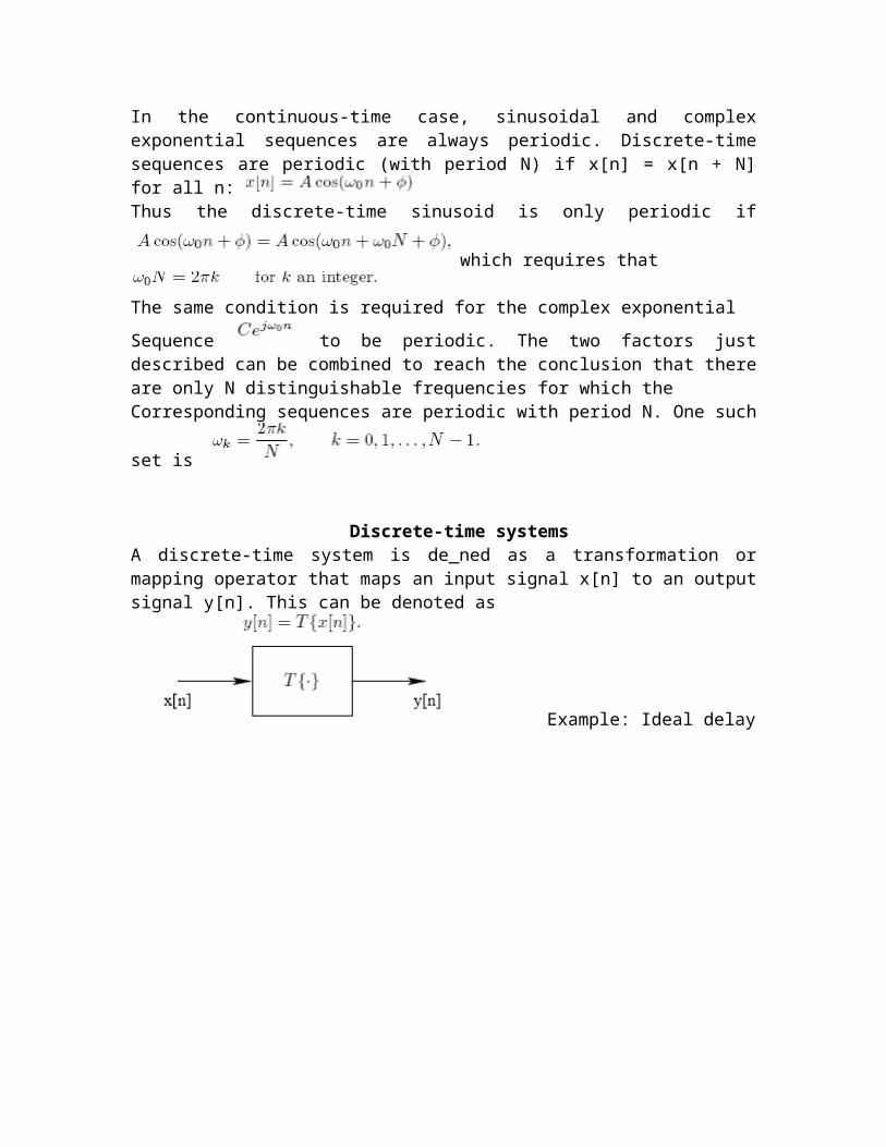
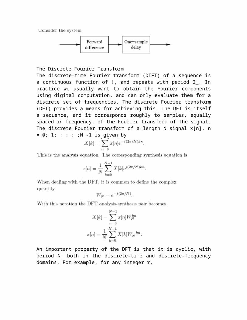
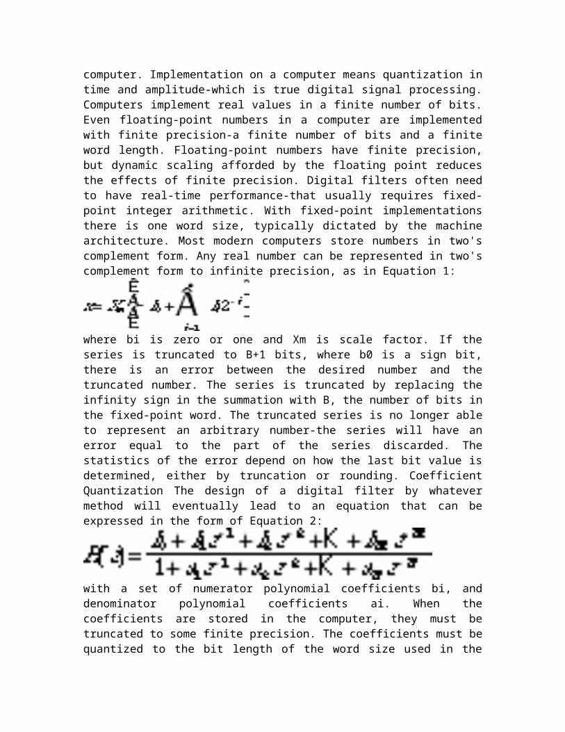
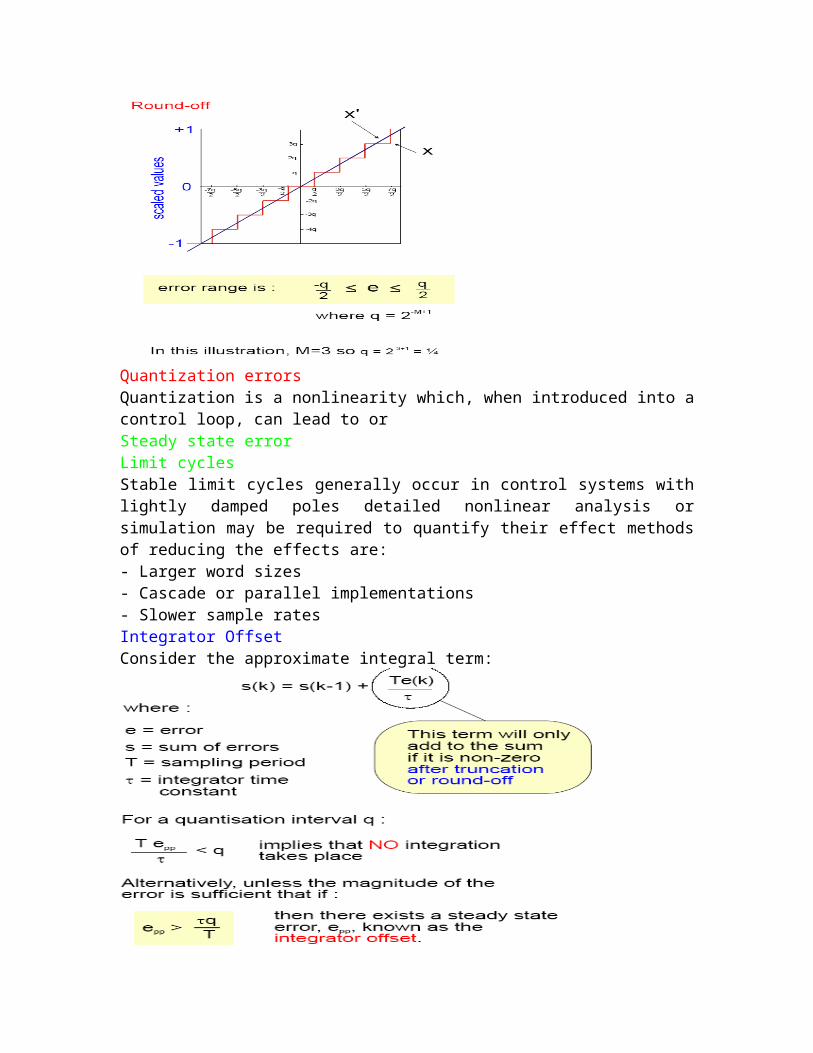
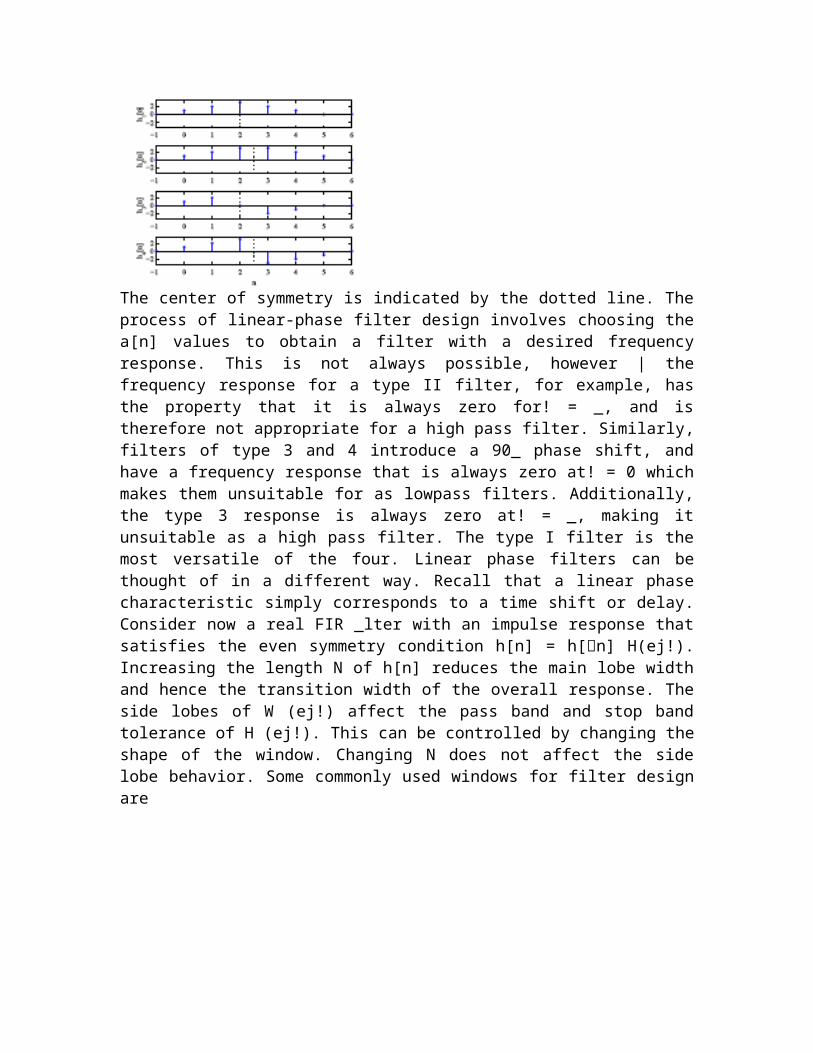