introduction to machine...
TRANSCRIPT
Introduction
to
Machine
Learning
Second
E d i t i o n
Ethem Alpaydın
The MIT PressCambridge, Massachusetts
London, England

© 2010 Massachusetts Institute of Technology
All rights reserved. No part of this book may be reproduced in any form by any
electronic or mechanical means (including photocopying, recording, or informa-
tion storage and retrieval) without permission in writing from the publisher.
For information about special quantity discounts, please email
Typeset in 10/13 Lucida Bright by the author using LATEX2ε .
Printed and bound in the United States of America.
Library of Congress Cataloging-in-Publication Information
Alpaydin, Ethem.
Introduction to machine learning / Ethem Alpaydin. — 2nd ed.p. cm.
Includes bibliographical references and index.ISBN 978-0-262-01243-0 (hardcover : alk. paper)1. Machine learning. I. Title
Q325.5.A46 2010006.3’1—dc22 2009013169
CIP
10 9 8 7 6 5 4 3 2 1
Brief Contents
1 Introduction 1
2 Supervised Learning 21
3 Bayesian Decision Theory 47
4 Parametric Methods 61
5 Multivariate Methods 87
6 Dimensionality Reduction 109
7 Clustering 143
8 Nonparametric Methods 163
9 Decision Trees 185
10 Linear Discrimination 209
11 Multilayer Perceptrons 233
12 Local Models 279
13 Kernel Machines 309
14 Bayesian Estimation 341
15 Hidden Markov Models 363
16 Graphical Models 387
17 Combining Multiple Learners 419
18 Reinforcement Learning 447
19 Design and Analysis of Machine Learning Experiments 475
A Probability 517

x Contents
8.2.1 Histogram Estimator 1658.2.2 Kernel Estimator 1678.2.3 k-Nearest Neighbor Estimator 168
8.3 Generalization to Multivariate Data 1708.4 Nonparametric Classification 1718.5 Condensed Nearest Neighbor 1728.6 Nonparametric Regression: Smoothing Models 174
8.6.1 Running Mean Smoother 1758.6.2 Kernel Smoother 1768.6.3 Running Line Smoother 177
8.7 How to Choose the Smoothing Parameter 1788.8 Notes 1808.9 Exercises 1818.10 References 182
9 Decision Trees 185
9.1 Introduction 1859.2 Univariate Trees 187
9.2.1 Classification Trees 1889.2.2 Regression Trees 192
9.3 Pruning 1949.4 Rule Extraction from Trees 1979.5 Learning Rules from Data 1989.6 Multivariate Trees 2029.7 Notes 2049.8 Exercises 2079.9 References 207
10 Linear Discrimination 209
10.1 Introduction 20910.2 Generalizing the Linear Model 21110.3 Geometry of the Linear Discriminant 212
10.3.1 Two Classes 21210.3.2 Multiple Classes 214
10.4 Pairwise Separation 21610.5 Parametric Discrimination Revisited 21710.6 Gradient Descent 21810.7 Logistic Discrimination 220
10.7.1 Two Classes 220

Contents xi
10.7.2 Multiple Classes 22410.8 Discrimination by Regression 22810.9 Notes 23010.10 Exercises 23010.11 References 231
11 Multilayer Perceptrons 233
11.1 Introduction 23311.1.1 Understanding the Brain 23411.1.2 Neural Networks as a Paradigm for Parallel
Processing 23511.2 The Perceptron 23711.3 Training a Perceptron 24011.4 Learning Boolean Functions 24311.5 Multilayer Perceptrons 24511.6 MLP as a Universal Approximator 24811.7 Backpropagation Algorithm 249
11.7.1 Nonlinear Regression 25011.7.2 Two-Class Discrimination 25211.7.3 Multiclass Discrimination 25411.7.4 Multiple Hidden Layers 256
11.8 Training Procedures 25611.8.1 Improving Convergence 25611.8.2 Overtraining 25711.8.3 Structuring the Network 25811.8.4 Hints 261
11.9 Tuning the Network Size 26311.10 Bayesian View of Learning 26611.11 Dimensionality Reduction 26711.12 Learning Time 270
11.12.1 Time Delay Neural Networks 27011.12.2 Recurrent Networks 271
11.13 Notes 27211.14 Exercises 27411.15 References 275
12 Local Models 279
12.1 Introduction 27912.2 Competitive Learning 280

Preface
Machine learning is programming computers to optimize a performancecriterion using example data or past experience. We need learning incases where we cannot directly write a computer program to solve a givenproblem, but need example data or experience. One case where learningis necessary is when human expertise does not exist, or when humansare unable to explain their expertise. Consider the recognition of spokenspeech—that is, converting the acoustic speech signal to an ASCII text;we can do this task seemingly without any difficulty, but we are unableto explain how we do it. Different people utter the same word differentlydue to differences in age, gender, or accent. In machine learning, the ap-proach is to collect a large collection of sample utterances from differentpeople and learn to map these to words.
Another case is when the problem to be solved changes in time, ordepends on the particular environment. We would like to have general-purpose systems that can adapt to their circumstances, rather than ex-plicitly writing a different program for each special circumstance. Con-sider routing packets over a computer network. The path maximizingthe quality of service from a source to destination changes continuouslyas the network traffic changes. A learning routing program is able toadapt to the best path by monitoring the network traffic. Another ex-ample is an intelligent user interface that can adapt to the biometrics ofits user—namely, his or her accent, handwriting, working habits, and soforth.
Already, there are many successful applications of machine learningin various domains: There are commercially available systems for rec-ognizing speech and handwriting. Retail companies analyze their pastsales data to learn their customers’ behavior to improve customer rela-

xxxii Preface
tionship management. Financial institutions analyze past transactionsto predict customers’ credit risks. Robots learn to optimize their behav-ior to complete a task using minimum resources. In bioinformatics, thehuge amount of data can only be analyzed and knowledge extracted us-ing computers. These are only some of the applications that we—thatis, you and I—will discuss throughout this book. We can only imaginewhat future applications can be realized using machine learning: Carsthat can drive themselves under different road and weather conditions,phones that can translate in real time to and from a foreign language,autonomous robots that can navigate in a new environment, for example,on the surface of another planet. Machine learning is certainly an excitingfield to be working in!
The book discusses many methods that have their bases in differentfields: statistics, pattern recognition, neural networks, artificial intelli-gence, signal processing, control, and data mining. In the past, researchin these different communities followed different paths with differentemphases. In this book, the aim is to incorporate them together to give aunified treatment of the problems and the proposed solutions to them.
This is an introductory textbook, intended for senior undergraduateand graduate-level courses on machine learning, as well as engineersworking in the industry who are interested in the application of thesemethods. The prerequisites are courses on computer programming, prob-ability, calculus, and linear algebra. The aim is to have all learning algo-rithms sufficiently explained so it will be a small step from the equationsgiven in the book to a computer program. For some cases, pseudocodeof algorithms are also included to make this task easier.
The book can be used for a one-semester course by sampling from thechapters, or it can be used for a two-semester course, possibly by dis-cussing extra research papers; in such a case, I hope that the referencesat the end of each chapter are useful.
The Web page is http://www.cmpe.boun.edu.tr/∼ethem/i2ml/ where Iwill post information related to the book that becomes available after thebook goes to press, for example, errata. I welcome your feedback viaemail to [email protected].
I very much enjoyed writing this book; I hope you will enjoy reading it.

Notes for the Second Edition
Machine learning has seen important developments since the first editionappeared in 2004. First, application areas have grown rapidly. Internet-related technologies, such as search engines, recommendation systems,spam fiters, and intrusion detection systems are now routinely using ma-chine learning. In the field of bioinformatics and computational biology,methods that learn from data are being used more and more widely. Innatural language processing applications—for example, machine transla-tion—we are seeing a faster and faster move from programmed expertsystems to methods that learn automatically from very large corpus ofexample text. In robotics, medical diagnosis, speech and image recogni-tion, biometrics, finance, sometimes under the name pattern recognition,sometimes disguised as data mining, or under one of its many cloaks,we see more and more applications of the machine learning methods wediscuss in this textbook.
Second, there have been supporting advances in theory. Especially, theidea of kernel functions and the kernel machines that use them allowa better representation of the problem and the associated convex opti-mization framework is one step further than multilayer perceptrons withsigmoid hidden units trained using gradient-descent. Bayesian meth-ods through appropriately chosen prior distributions add expert know-ledge to what the data tells us. Graphical models allow a representa-tion as a network of interrelated nodes and efficient inference algorithmsallow querying the network. It has thus become necessary that thesethree topics—namely, kernel methods, Bayesian estimation, and graphi-cal models—which were sections in the first edition, be treated in morelength, as three new chapters.
Another revelation hugely significant for the field has been in the real-
xxxvi Notes for the Second Edition
ization that machine learning experiments need to be designed better. Wehave gone a long way from using a single test set to methods for cross-validation to paired t tests. That is why, in this second edition, I haverewritten the chapter on statistical tests as one that includes the designand analysis of machine learning experiments. The point is that testingshould not be a separate step done after all runs are completed (despitethe fact that this new chapter is at the very end of the book); the wholeprocess of experimentation should be designed beforehand, relevant fac-tors defined, proper experimentation procedure decided upon, and then,and only then, the runs should be done and the results analyzed.
It has long been believed, especially by older members of the scientificcommunity, that for machines to be as intelligent as us, that is, for ar-tificial intelligence to be a reality, our current knowledge in general, orcomputer science in particular, is not sufficient. People largely are ofthe opinion that we need a new technology, a new type of material, anew type of computational mechanism or a new programming methodol-ogy, and that, until then, we can only “simulate” some aspects of humanintelligence and only in a limited way but can never fully attain it.
I believe that we will soon prove them wrong. First we saw this inchess, and now we are seeing it in a whole variety of domains. Givenenough memory and computation power, we can realize tasks with rela-tively simple algorithms; the trick here is learning, either learning fromexample data or learning from trial and error using reinforcement learn-ing. It seems as if using supervised and mostly unsupervised learn-ing algorithms—for example, machine translation—will soon be possible.The same holds for many other domains, for example, unmanned navi-gation in robotics using reinforcement learning. I believe that this willcontinue for many domains in artificial intelligence, and the key is learn-ing. We do not need to come up with new algorithms if machines canlearn themselves, assuming that we can provide them with enough data(not necessarily supervised) and computing power.
I would like to thank all the instructors and students of the first edition,from all over the world, including the reprint in India and the Germantranslation. I am grateful to those who sent me words of appreciationand errata or who provided feedback in any other way. Please keep thoseemails coming. My email address is [email protected].
The second edition also provides more support on the Web. The book’s

Notes for the Second Edition xxxvii
Web site is http://www.cmpe.boun.edu.tr/∼ethem/i2ml.
I would like to thank my past and present thesis students, Mehmet Gönen,Esma Kılıç, Murat Semerci, M. Aydın Ulas, and Olcay Taner Yıldız, and alsothose who have taken CmpE 544, CmpE 545, CmpE 591, and CmpE 58Eduring these past few years. The best way to test your knowledge of atopic is by teaching it.
It has been a pleasure working with the MIT Press again on this secondedition, and I thank Bob Prior, Ada Brunstein, Erin K. Shoudy, KathleenCaruso, and Marcy Ross for all their help and support.
Notations
x Scalar value
x Vector
X Matrix
xT Transpose
X−1 Inverse
X Random variable
P(X) Probability mass function when X is discrete
p(X) Probability density function when X is continuous
P(X|Y) Conditional probability of X given Y
E[X] Expected value of the random variable X
Var(X) Variance of X
Cov(X, Y) Covariance of X and Y
Corr(X, Y) Correlation of X and Y
µ Mean
σ 2 Variance
Σ Covariance matrix
m Estimator to the mean
s2 Estimator to the variance
S Estimator to the covariance matrix

xl Notations
N (µ,σ 2) Univariate normal distribution with mean µ and vari-ance σ 2
Z Unit normal distribution: N (0,1)
Nd(µ,Σ) d-variate normal distribution with mean vector µ andcovariance matrix Σ
x Input
d Number of inputs (input dimensionality)
y Output
r Required output
K Number of outputs (classes)
N Number of training instances
z Hidden value, intrinsic dimension, latent factor
k Number of hidden dimensions, latent factors
Ci Class i
X Training sample
{xt}Nt=1 Set of x with index t ranging from 1 to N
{xt, r t}t Set of ordered pairs of input and desired output withindex t
g(x|θ) Function of x defined up to a set of parameters θ
arg maxθ g(x|θ) The argument θ for which g has its maximum value
arg minθ g(x|θ) The argument θ for which g has its minimum value
E(θ|X) Error function with parameters θ on the sample Xl(θ|X) Likelihood of parameters θ on the sample XL(θ|X) Log likelihood of parameters θ on the sample X
1(c) 1 if c is true, 0 otherwise
#{c} Number of elements for which c is true
δij Kronecker delta: 1 if i = j , 0 otherwise

11 Multilayer Perceptrons
The multilayer perceptron is an artificial neural network structure
and is a nonparametric estimator that can be used for classification
and regression. We discuss the backpropagation algorithm to train
a multilayer perceptron for a variety of applications.
11.1 Introduction
Artificial neural network models, one of which is the perceptron
we discuss in this chapter, take their inspiration from the brain. Thereare cognitive scientists and neuroscientists whose aim is to understandthe functioning of the brain (Posner 1989; Thagard 2005), and towardthis aim, build models of the natural neural networks in the brain andmake simulation studies.
However, in engineering, our aim is not to understand the brain perse, but to build useful machines. We are interested in artificial neuralartificial neural
networks networks because we believe that they may help us build better computersystems. The brain is an information processing device that has someincredible abilities and surpasses current engineering products in manydomains—for example, vision, speech recognition, and learning, to namethree. These applications have evident economic utility if implementedon machines. If we can understand how the brain performs these func-tions, we can define solutions to these tasks as formal algorithms andimplement them on computers.
The human brain is quite different from a computer. Whereas a com-puter generally has one processor, the brain is composed of a very large(1011) number of processing units, namely, neurons, operating in parallel.neurons
Though the details are not known, the processing units are believed to be

234 11 Multilayer Perceptrons
much simpler and slower than a processor in a computer. What alsomakes the brain different, and is believed to provide its computationalpower, is the large connectivity. Neurons in the brain have connections,called synapses, to around 104 other neurons, all operating in parallel.synapses
In a computer, the processor is active and the memory is separate andpassive, but it is believed that in the brain, both the processing and mem-ory are distributed together over the network; processing is done by theneurons, and the memory is in the synapses between the neurons.
11.1.1 Understanding the Brain
According to Marr (1982), understanding an information processing sys-tem has three levels, called the levels of analysis:levels of analysis
1. Computational theory corresponds to the goal of computation and anabstract definition of the task.
2. Representation and algorithm is about how the input and the outputare represented and about the specification of the algorithm for thetransformation from the input to the output.
3. Hardware implementation is the actual physical realization of the sys-tem.
One example is sorting: The computational theory is to order a givenset of elements. The representation may use integers, and the algorithmmay be Quicksort. After compilation, the executable code for a particularprocessor sorting integers represented in binary is one hardware imple-mentation.
The idea is that for the same computational theory, there may be mul-tiple representations and algorithms manipulating symbols in that repre-sentation. Similarly, for any given representation and algorithm, theremay be multiple hardware implementations. We can use one of vari-ous sorting algorithms, and even the same algorithm can be compiledon computers with different processors and lead to different hardwareimplementations.
To take another example, ‘6’, ‘VI’, and ‘110’ are three different repre-sentations of the number six. There is a different algorithm for additiondepending on the representation used. Digital computers use binary rep-resentation and have circuitry to add in this representation, which is one

11.1 Introduction 235
particular hardware implementation. Numbers are represented differ-ently, and addition corresponds to a different set of instructions on anabacus, which is another hardware implementation. When we add twonumbers in our head, we use another representation and an algorithmsuitable to that representation, which is implemented by the neurons. Butall these different hardware implementations—for example, us, abacus,digital computer—implement the same computational theory, addition.
The classic example is the difference between natural and artificial fly-ing machines. A sparrow flaps its wings; a commercial airplane does notflap its wings but uses jet engines. The sparrow and the airplane aretwo hardware implementations built for different purposes, satisfyingdifferent constraints. But they both implement the same theory, which isaerodynamics.
The brain is one hardware implementation for learning or pattern recog-nition. If from this particular implementation, we can do reverse engi-neering and extract the representation and the algorithm used, and iffrom that in turn, we can get the computational theory, we can then useanother representation and algorithm, and in turn a hardware implemen-tation more suited to the means and constraints we have. One hopes ourimplementation will be cheaper, faster, and more accurate.
Just as the initial attempts to build flying machines looked very muchlike birds until we discovered aerodynamics, it is also expected that thefirst attempts to build structures possessing brain’s abilities will looklike the brain with networks of large numbers of processing units, untilwe discover the computational theory of intelligence. So it can be saidthat in understanding the brain, when we are working on artificial neuralnetworks, we are at the representation and algorithm level.
Just as the feathers are irrelevant to flying, in time we may discoverthat neurons and synapses are irrelevant to intelligence. But until thattime there is one other reason why we are interested in understandingthe functioning of the brain, and that is related to parallel processing.
11.1.2 Neural Networks as a Paradigm for Parallel Processing
Since the 1980s, computer systems with thousands of processors havebeen commercially available. The software for such parallel architectures,however, has not advanced as quickly as hardware. The reason for thisis that almost all our theory of computation up to that point was based

236 11 Multilayer Perceptrons
on serial, one-processor machines. We are not able to use the parallelmachines we have efficiently because we cannot program them efficiently.
There are mainly two paradigms for parallel processing: In Single In-parallel processing
struction Multiple Data (SIMD) machines, all processors execute the sameinstruction but on different pieces of data. In Multiple Instruction Mul-tiple Data (MIMD) machines, different processors may execute differentinstructions on different data. SIMD machines are easier to program be-cause there is only one program to write. However, problems rarely havesuch a regular structure that they can be parallelized over a SIMD ma-chine. MIMD machines are more general, but it is not an easy task to writeseparate programs for all the individual processors; additional problemsare related to synchronization, data transfer between processors, and soforth. SIMD machines are also easier to build, and machines with moreprocessors can be constructed if they are SIMD. In MIMD machines, pro-cessors are more complex, and a more complex communication networkshould be constructed for the processors to exchange data arbitrarily.
Assume now that we can have machines where processors are a lit-tle bit more complex than SIMD processors but not as complex as MIMDprocessors. Assume we have simple processors with a small amount oflocal memory where some parameters can be stored. Each processor im-plements a fixed function and executes the same instructions as SIMDprocessors; but by loading different values into the local memory, theycan be doing different things and the whole operation can be distributedover such processors. We will then have what we can call Neural Instruc-tion Multiple Data (NIMD) machines, where each processor correspondsto a neuron, local parameters correspond to its synaptic weights, and thewhole structure is a neural network. If the function implemented in eachprocessor is simple and if the local memory is small, then many suchprocessors can be fit on a single chip.
The problem now is to distribute a task over a network of such proces-sors and to determine the local parameter values. This is where learningcomes into play: We do not need to program such machines and deter-mine the parameter values ourselves if such machines can learn fromexamples.
Thus, artificial neural networks are a way to make use of the parallelhardware we can build with current technology and—thanks to learning—they need not be programmed. Therefore, we also save ourselves theeffort of programming them.
In this chapter, we discuss such structures and how they are trained.

11.2 The Perceptron 237
Figure 11.1 Simple perceptron. xj , j = 1, . . . , d are the input units. x0 is thebias unit that always has the value 1. y is the output unit. wj is the weight ofthe directed connection from input xj to the output.
Keep in mind that the operation of an artificial neural network is a math-ematical function that can be implemented on a serial computer—as itgenerally is—and training the network is not much different from statisti-cal techniques that we have discussed in the previous chapters. Thinkingof this operation as being carried out on a network of simple processingunits is meaningful only if we have the parallel hardware, and only if thenetwork is so large that it cannot be simulated fast enough on a serialcomputer.
11.2 The Perceptron
The perceptron is the basic processing element. It has inputs that mayperceptron
come from the environment or may be the outputs of other perceptrons.Associated with each input, xj ∈ ℜ, j = 1, . . . , d, is a connection weight,connection weight
or synaptic weight wj ∈ ℜ, and the output, y , in the simplest case is asynaptic weight
weighted sum of the inputs (see figure 11.1):
y =d∑
j=1
wjxj +w0(11.1)
w0 is the intercept value to make the model more general; it is generallymodeled as the weight coming from an extra bias unit, x0, which is alwaysbias unit

238 11 Multilayer Perceptrons
+1. We can write the output of the perceptron as a dot product
y = wTx(11.2)
where w = [w0, w1, . . . , wd]T and x = [1, x1, . . . , xd]T are augmented vec-tors to include also the bias weight and input.
During testing, with given weights, w, for input x, we compute theoutput y . To implement a given task, we need to learn the weights w, theparameters of the system, such that correct outputs are generated giventhe inputs.
When d = 1 and x is fed from the environment through an input unit,we have
y = wx+w0
which is the equation of a line with w as the slope and w0 as the inter-cept. Thus this perceptron with one input and one output can be usedto implement a linear fit. With more than one input, the line becomes a(hyper)plane, and the perceptron with more than one input can be usedto implement multivariate linear fit. Given a sample, the parameters wjcan be found by regression (see section 5.8).
The perceptron as defined in equation 11.1 defines a hyperplane and assuch can be used to divide the input space into two: the half-space whereit is positive and the half-space where it is negative (see chapter 10). Byusing it to implement a linear discriminant function, the perceptron canseparate two classes by checking the sign of the output. If we define s(·)as the threshold functionthreshold function
s(a) ={
1 if a > 00 otherwise
(11.3)
then we can
choose
{
C1 if s(wTx) > 0C2 otherwise
Remember that using a linear discriminant assumes that classes arelinearly separable. That is to say, it is assumed that a hyperplanewTx = 0can be found that separates xt ∈ C1 and xt ∈ C2. If at a later stage weneed the posterior probability—for example, to calculate risk—we needto use the sigmoid function at the output as
o = wTx
y = sigmoid(o) = 1
1+ exp[−wTx](11.4)

11.2 The Perceptron 239
Figure 11.2 K parallel perceptrons. xj , j = 0, . . . , d are the inputs and yi, i =1, . . . , K are the outputs. wij is the weight of the connection from input xj tooutput yi . Each output is a weighted sum of the inputs. When used for K-classclassification problem, there is a postprocessing to choose the maximum, orsoftmax if we need the posterior probabilities.
When there are K > 2 outputs, there are K perceptrons, each of whichhas a weight vector wi (see figure 11.2)
yi =d∑
j=1
wijxj +wi0 = wTi x
y = Wx(11.5)
where wij is the weight from input xj to output yi . W is the K × (d + 1)weight matrix of wij whose rows are the weight vectors of the K percep-trons. When used for classification, during testing, we
choose Ci if yi = maxkyk
In the case of a neural network, the value of each perceptron is a local
function of its inputs and its synaptic weights. However, in classification,if we need the posterior probabilities (instead of just the code of thewinner class) and use the softmax, we also need the values of the otheroutputs. So, to implement this as a neural network, we can see this asa two-stage process, where the first stage calculates the weighted sums,and the second stage calculates the softmax values; but we still denote

240 11 Multilayer Perceptrons
this as a single layer of output units:
oi = wTi x
yi = expoi∑
k expok(11.6)
Remember that by defining auxiliary inputs, the linear model can alsobe used for polynomial approximation; for example, define x3 = x2
1, x4 =x2
2, x5 = x1x2 (section 10.2). The same can also be used with perceptrons(Durbin and Rumelhart 1989). In section 11.5, we see multilayer percep-trons where such nonlinear functions are learned from data in a “hidden”layer instead of being assumed a priori.
Any of the methods discussed in chapter 10 on linear discriminationcan be used to calculate wi , i = 1, . . . , K offline and then plugged into thenetwork. These include parametric approach with a common covariancematrix, logistic discrimination, discrimination by regression, and supportvector machines. In some cases, we do not have the whole sample at handwhen training starts, and we need to iteratively update parameters as newexamples arrive; we discuss this case of online learning in section 11.3.
Equation 11.5 defines a linear transformation from a d-dimensionalspace to a K-dimensional space and can also be used for dimensional-ity reduction if K < d. One can use any of the methods of chapter 6 tocalculate W offline and then use the perceptrons to implement the trans-formation, for example, PCA. In such a case, we have a two-layer networkwhere the first layer of perceptrons implements the linear transformationand the second layer implements the linear regression or classification inthe new space. We note that because both are linear transformations,they can be combined and written down as a single layer. We will see themore interesting case where the first layer implements nonlinear dimen-sionality reduction in section 11.5.
11.3 Training a Perceptron
The perceptron defines a hyperplane, and the neural network perceptronis just a way of implementing the hyperplane. Given a data sample, theweight values can be calculated offline and then when they are pluggedin, the perceptron can be used to calculate the output values.
In training neural networks, we generally use online learning where weare not given the whole sample, but we are given instances one by oneand would like the network to update its parameters after each instance,

11.3 Training a Perceptron 241
adapting itself slowly in time. Such an approach is interesting for a num-ber of reasons:
1. It saves us the cost of storing the training sample in an external mem-ory and storing the intermediate results during optimization. An ap-proach like support vector machines (chapter 13) may be quite costlywith large samples, and in some applications, we may prefer a simplerapproach where we do not need to store the whole sample and solve acomplex optimization problem on it.
2. The problem may be changing in time, which means that the sampledistribution is not fixed, and a training set cannot be chosen a priori.For example, we may be implementing a speech recognition systemthat adapts itself to its user.
3. There may be physical changes in the system. For example, in a roboticsystem, the components of the system may wear out, or sensors maydegrade.
In online learning, we do not write the error function over the wholeonline learning
sample but on individual instances. Starting from random initial weights,at each iteration we adjust the parameters a little bit to minimize theerror, without forgetting what we have previously learned. If this errorfunction is differentiable, we can use gradient descent.
For example, in regression the error on the single instance pair withindex t , (xt , r t ), is
Et(w|xt , r t ) = 1
2(r t − yt)2 = 1
2[r t − (wTxt)]2
and for j = 0, . . . , d, the online update is
∆wtj = η(r t − yt)xtj(11.7)
where η is the learning factor, which is gradually decreased in time forconvergence. This is known as stochastic gradient descent.stochastic
gradient descent Similarly, update rules can be derived for classification problems usinglogistic discrimination where updates are done after each pattern, insteadof summing them and doing the update after a complete pass over thetraining set. With two classes, for the single instance (xt , r t) where r ti = 1if xt ∈ C1 and r ti = 0 if xt ∈ C2, the single output is
yt = sigmoid(wTxt )

242 11 Multilayer Perceptrons
and the cross-entropy is
Et(w|xt , r t ) = −r t logyt − (1− r t ) log(1− yt)
Using gradient descent, we get the following online update rule forj = 0, . . . , d:
∆wtj = η(r t − yt)xtj(11.8)
When there are K > 2 classes, for the single instance (xt , r t ) wherer ti = 1 if xt ∈ Ci and 0 otherwise, the outputs are
yti =expwT
i xt
∑
k expwTkx
t
and the cross-entropy is
Et({wi}i|xt , r t) = −∑
i
r ti logyti
Using gradient descent, we get the following online update rule, fori = 1, . . . , K, j = 0, . . . , d:
∆wtij = η(r ti − yti )xtj(11.9)
which is the same as the equations we saw in section 10.7 except that wedo not sum over all of the instances but update after a single instance.The pseudocode of the algorithm is given in figure 11.3, which is theonline version of figure 10.8.
Both equations 11.7 and 11.9 have the form
Update = LearningFactor· (DesiredOutput − ActualOutput) · Input(11.10)
Let us try to get some insight into what this does. First, if the actualoutput is equal to the desired output, no update is done. When it isdone, the magnitude of the update increases as the difference betweenthe desired output and the actual output increases. We also see that ifthe actual output is less than the desired output, update is positive ifthe input is positive and negative if the input is negative. This has theeffect of increasing the actual output and decreasing the difference. Ifthe actual output is greater than the desired output, update is negative ifthe input is positive and positive if the input is negative; this decreasesthe actual output and makes it closer to the desired output.

11.4 Learning Boolean Functions 243
For i = 1, . . . , KFor j = 0, . . . , d
wij ← rand(−0.01,0.01)
Repeat
For all (xt , r t ) ∈ X in random order
For i = 1, . . . , Koi ← 0For j = 0, . . . , d
oi ← oi +wijxtjFor i = 1, . . . , K
yi ← exp(oi)/∑
k exp(ok)For i = 1, . . . , K
For j = 0, . . . , dwij ← wij + η(r ti − yi)xtj
Until convergence
Figure 11.3 Perceptron training algorithm implementing stochastic online gra-dient descent for the case with K > 2 classes. This is the online version of thealgorithm given in figure 10.8.
When an update is done, its magnitude depends also on the input. Ifthe input is close to 0, its effect on the actual output is small and there-fore its weight is also updated by a small amount. The greater an input,the greater the update of its weight.
Finally, the magnitude of the update depends on the learning factor, η.If it is too large, updates depend too much on recent instances; it is as ifthe system has a very short memory. If this factor is small, many updatesmay be needed for convergence. In section 11.8.1, we discuss methods tospeed up convergence.
11.4 Learning Boolean Functions
In a Boolean function, the inputs are binary and the output is 1 if thecorresponding function value is true and 0 otherwise. Therefore, it canbe seen as a two-class classification problem. As an example, for learningto AND two inputs, the table of inputs and required outputs is given intable 11.1. An example of a perceptron that implements AND and its

244 11 Multilayer Perceptrons
Table 11.1 Input and output for the AND function.
x1 x2 r
0 0 00 1 01 0 01 1 1
x0=+1 x1 x2
y
-1.5+1+1
x1
x2
+
(0,0)
(1,1)
(1,0)
(0,1)
1.5
1.5
Figure 11.4 The perceptron that implements AND and its geometric interpre-tation.
geometric interpretation in two dimensions is given in figure 11.4. Thediscriminant is
y = s(x1 + x2 − 1.5)
that is, x = [1, x1, x2]T andw = [−1.5,1,1]T . Note that y = s(x1+x2−1.5)satisfies the four constraints given by the definition of AND function intable 11.1, for example, for x1 = 1, x2 = 0, y = s(−0.5) = 0. Similarly itcan be shown that y = s(x1 + x2 − 0.5) implements OR.
Though Boolean functions like AND and OR are linearly separable andare solvable using the perceptron, certain functions like XOR are not. Thetable of inputs and required outputs for XOR is given in table 11.2. Ascan be seen in figure 11.5, the problem is not linearly separable. Thiscan also be proved by noting that there are no w0, w1, and w2 values that
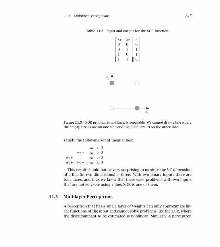
11.5 Multilayer Perceptrons 245
Table 11.2 Input and output for the XOR function.
x1 x2 r
0 0 00 1 11 0 11 1 0
x1
x2
Figure 11.5 XOR problem is not linearly separable. We cannot draw a line wherethe empty circles are on one side and the filled circles on the other side.
satisfy the following set of inequalities:
w0 ≤ 0w2+ w0 > 0
w1+ w0 > 0w1+ w2+ w0 ≤ 0
This result should not be very surprising to us since the VC dimensionof a line (in two dimensions) is three. With two binary inputs there arefour cases, and thus we know that there exist problems with two inputsthat are not solvable using a line; XOR is one of them.
11.5 Multilayer Perceptrons
A perceptron that has a single layer of weights can only approximate lin-ear functions of the input and cannot solve problems like the XOR, wherethe discrimininant to be estimated is nonlinear. Similarly, a perceptron

246 11 Multilayer Perceptrons
cannot be used for nonlinear regression. This limitation does not applyto feedforward networks with intermediate or hidden layers between thehidden layers
input and the output layers. If used for classification, such multilayermultilayer
perceptrons perceptrons (MLP) can implement nonlinear discriminants and, if usedfor regression, can approximate nonlinear functions of the input.
Input x is fed to the input layer (including the bias), the “activation”propagates in the forward direction, and the values of the hidden unitszh are calculated (see figure 11.6). Each hidden unit is a perceptron byitself and applies the nonlinear sigmoid function to its weighted sum:
zh = sigmoid(wThx) =
1
1+ exp[
−(∑dj=1whjxj +wh0
)] , h = 1, . . . ,H(11.11)
The output yi are perceptrons in the second layer taking the hiddenunits as their inputs
yi = vTi z =H∑
h=1
vihzh + vi0(11.12)
where there is also a bias unit in the hidden layer, which we denote by z0,and vi0 are the bias weights. The input layer of xj is not counted sinceno computation is done there and when there is a hidden layer, this is atwo-layer network.
As usual, in a regression problem, there is no nonlinearity in the outputlayer in calculating y . In a two-class discrimination task, there is one sig-moid output unit and when there are K > 2 classes, there are K outputswith softmax as the output nonlinearity.
If the hidden units’ outputs were linear, the hidden layer would be of nouse: linear combination of linear combinations is another linear combi-nation. Sigmoid is the continuous, differentiable version of thresholding.We need differentiability because the learning equations we will see aregradient-based. Another sigmoid (S-shaped) nonlinear basis function thatcan be used is the hyperbolic tangent function, tanh, which ranges from−1 to +1, instead of 0 to +1. In practice, there is no difference betweenusing the sigmoid and the tanh. Still another possibility is the Gaussian,which uses Euclidean distance instead of the dot product for similarity;we discuss such radial basis function networks in chapter 12.
The output is a linear combination of the nonlinear basis function val-ues computed by the hidden units. It can be said that the hidden unitsmake a nonlinear transformation from the d-dimensional input space to
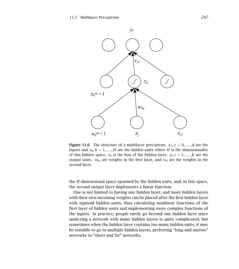
11.5 Multilayer Perceptrons 247
Figure 11.6 The structure of a multilayer perceptron. xj , j = 0, . . . , d are theinputs and zh, h = 1, . . . , H are the hidden units where H is the dimensionalityof this hidden space. z0 is the bias of the hidden layer. yi, i = 1, . . . , K are theoutput units. whj are weights in the first layer, and vih are the weights in thesecond layer.
the H-dimensional space spanned by the hidden units, and, in this space,the second output layer implements a linear function.
One is not limited to having one hidden layer, and more hidden layerswith their own incoming weights can be placed after the first hidden layerwith sigmoid hidden units, thus calculating nonlinear functions of thefirst layer of hidden units and implementing more complex functions ofthe inputs. In practice, people rarely go beyond one hidden layer sinceanalyzing a network with many hidden layers is quite complicated; butsometimes when the hidden layer contains too many hidden units, it maybe sensible to go to multiple hidden layers, preferring “long and narrow”networks to “short and fat” networks.
248 11 Multilayer Perceptrons
11.6 MLP as a Universal Approximator
We can represent any Boolean function as a disjunction of conjunctions,and such a Boolean expression can be implemented by a multilayer per-ceptron with one hidden layer. Each conjunction is implemented by onehidden unit and the disjunction by the output unit. For example,
x1 XOR x2 = (x1 AND ∼ x2) OR (∼ x1 AND x2)
We have seen previously how to implement AND and OR using percep-trons. So two perceptrons can in parallel implement the two AND, andanother perceptron on top can OR them together (see figure 11.7). We seethat the first layer maps inputs from the (x1, x2) to the (z1, z2) space de-fined by the first-layer perceptrons. Note that both inputs, (0,0) and (1,1),are mapped to (0,0) in the (z1, z2) space, allowing linear separability inthis second space.
Thus in the binary case, for every input combination where the outputis 1, we define a hidden unit that checks for that particular conjunction ofthe input. The output layer then implements the disjunction. Note thatthis is just an existence proof, and such networks may not be practicalas up to 2d hidden units may be necessary when there are d inputs. Suchan architecture implements table lookup and does not generalize.
We can extend this to the case where inputs are continuous to showthat similarly, any arbitrary function with continuous input and outputscan be approximated with a multilayer perceptron. The proof of universaluniversal
approximation approximation is easy with two hidden layers. For every input case orregion, that region can be delimited by hyperplanes on all sides usinghidden units on the first hidden layer. A hidden unit in the second layerthen ANDs them together to bound the region. We then set the weightof the connection from that hidden unit to the output unit equal to thedesired function value. This gives a piecewise constant approximationpiecewise constant
approximation of the function; it corresponds to ignoring all the terms in the Taylorexpansion except the constant term. Its accuracy may be increased tothe desired value by increasing the number of hidden units and placinga finer grid on the input. Note that no formal bounds are given on thenumber of hidden units required. This property just reassures us thatthere is a solution; it does not help us in any other way. It has been proventhat an MLP with one hidden layer (with an arbitrary number of hiddenunits) can learn any nonlinear function of the input (Hornik, Stinchcombe,and White 1989).

11.7 Backpropagation Algorithm 249
x0=+1 x1 x2
y
z1
z0=+1
z2
-0.5 -1 +1-1+1-0.5
+1 +1 -0.5
z1
z2
+
+
+
x1
x2
z1
z2y
Figure 11.7 The multilayer perceptron that solves the XOR problem. The hid-den units and the output have the threshold activation function with thresholdat 0.
11.7 Backpropagation Algorithm
Training a multilayer perceptron is the same as training a perceptron;the only difference is that now the output is a nonlinear function of theinput thanks to the nonlinear basis function in the hidden units. Con-sidering the hidden units as inputs, the second layer is a perceptron andwe already know how to update the parameters, vij , in this case, giventhe inputs zh. For the first-layer weights, whj , we use the chain rule tocalculate the gradient:
∂E
∂whj= ∂E
∂yi
∂yi∂zh
∂zh∂whj

250 11 Multilayer Perceptrons
It is as if the error propagates from the output y back to the inputsand hence the name backpropagation was coined (Rumelhart, Hinton, andbackpropagation
Williams 1986a).
11.7.1 Nonlinear Regression
Let us first take the case of nonlinear regression (with a single output)calculated as
yt =H∑
h=1
vhzth + v0(11.13)
with zh computed by equation 11.11. The error function over the wholesample in regression is
E(W,v|X) = 1
2
∑
t
(r t − yt)2(11.14)
The second layer is a perceptron with hidden units as the inputs, andwe use the least-squares rule to update the second-layer weights:
∆vh = η∑
t
(r t − yt)zth(11.15)
The first layer are also perceptrons with the hidden units as the outputunits but in updating the first-layer weights, we cannot use the least-squares rule directly as we do not have a desired output specified for thehidden units. This is where the chain rule comes into play. We write
∆whj = −η ∂E
∂whj
= −η∑
t
∂Et
∂yt∂yt
∂zth
∂zth∂whj
= −η∑
t
−(r t − yt)︸ ︷︷ ︸
∂Et/∂yt
vh︸︷︷︸
∂yt /∂zth
zth(1− zth)xtj︸ ︷︷ ︸
∂zth/∂whj
= η∑
t
(r t − yt)vhzth(1− zth)xtj(11.16)
The product of the first two terms (rt−yt)vh acts like the error term forhidden unit h. This error is backpropagated from the error to the hiddenunit. (r t − yt) is the error in the output, weighted by the “responsibility”of the hidden unit as given by its weight vh. In the third term, zh(1− zh)

11.7 Backpropagation Algorithm 251
is the derivative of the sigmoid and xtj is the derivative of the weightedsum with respect to the weight whj . Note that the change in the first-layer weight, ∆whj , makes use of the second-layer weight, vh. Therefore,we should calculate the changes in both layers and update the first-layerweights, making use of the old value of the second-layer weights, thenupdate the second-layer weights.
Weights, whj , vh are started from small random values initially, for ex-ample, in the range [−0.01,0.01], so as not to saturate the sigmoids. It isalso a good idea to normalize the inputs so that they all have 0 mean andunit variance and have the same scale, since we use a single η parameter.
With the learning equations given here, for each pattern, we computethe direction in which each parameter needs be changed and the magni-tude of this change. In batch learning, we accumulate these changes overbatch learning
all patterns and make the change once after a complete pass over thewhole training set is made, as shown in the previous update equations.
It is also possible to have online learning, by updating the weights af-ter each pattern, thereby implementing stochastic gradient descent. Acomplete pass over all the patterns in the training set is called an epoch.epoch
The learning factor, η, should be chosen smaller in this case and patternsshould be scanned in a random order. Online learning converges fasterbecause there may be similar patterns in the dataset, and the stochastic-ity has an effect like adding noise and may help escape local minima.
An example of training a multilayer perceptron for regression is shownin figure 11.8. As training continues, the MLP fit gets closer to the under-lying function and error decreases (see figure 11.9). Figure 11.10 showshow the MLP fit is formed as a sum of the outputs of the hidden units.
It is also possible to have multiple output units, in which case a numberof regression problems are learned at the same time. We have
yti =H∑
h=1
vihzth + vi0(11.17)
and the error is
E(W,V|X) = 1
2
∑
t
∑
i
(r ti − yti )2(11.18)
The batch update rules are then
∆vih = η∑
t
(r ti − yti )zth(11.19)
252 11 Multilayer Perceptrons
−0.5 −0.4 −0.3 −0.2 −0.1 0 0.1 0.2 0.3 0.4 0.5−2
−1.5
−1
−0.5
0
0.5
1
1.5
2
100
200300
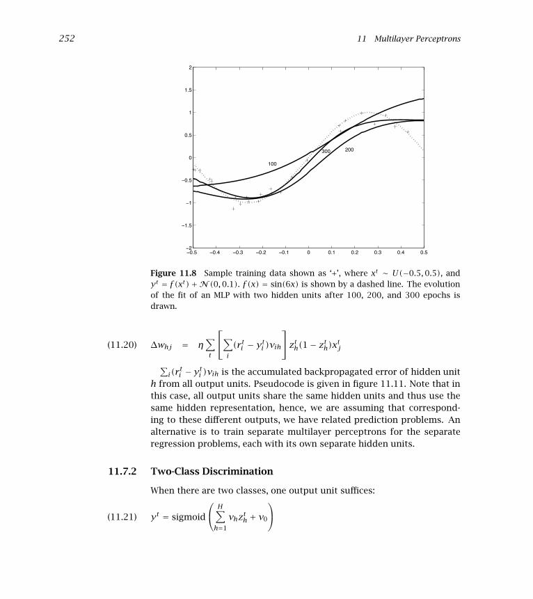
Figure 11.8 Sample training data shown as ‘+’, where xt ∼ U(−0.5,0.5), andyt = f (xt)+N (0,0.1). f (x) = sin(6x) is shown by a dashed line. The evolutionof the fit of an MLP with two hidden units after 100, 200, and 300 epochs isdrawn.
∆whj = η∑
t
⎡
⎣
∑
i
(r ti − yti )vih
⎤
⎦ zth(1− zth)xtj(11.20)
∑
i(rti − yti )vih is the accumulated backpropagated error of hidden unit
h from all output units. Pseudocode is given in figure 11.11. Note that inthis case, all output units share the same hidden units and thus use thesame hidden representation, hence, we are assuming that correspond-ing to these different outputs, we have related prediction problems. Analternative is to train separate multilayer perceptrons for the separateregression problems, each with its own separate hidden units.
11.7.2 Two-Class Discrimination
When there are two classes, one output unit suffices:
yt = sigmoid
⎛
⎝
H∑
h=1
vhzth + v0
⎞
⎠(11.21)

11.7 Backpropagation Algorithm 253
0 50 100 150 200 250 3000
0.2
0.4
0.6
0.8
1
1.2
1.4
Training Epochs
Mean
Squ
are E
rror
TrainingValidation
Figure 11.9 The mean square error on training and validation sets as a functionof training epochs.
which approximates P(C1|xt ) and P(C2|xt ) ≡ 1− yt . We remember fromsection 10.7 that the error function in this case is
E(W,v|X) = −∑
t
r t logyt + (1− r t ) log(1− yt)(11.22)
The update equations implementing gradient descent are
∆vh = η∑
t
(r t − yt)zth(11.23)
∆whj = η∑
t
(r t − yt)vhzth(1− zth)xtj(11.24)
As in the simple perceptron, the update equations for regression andclassification are identical (which does not mean that the values are).

254 11 Multilayer Perceptrons
−0.5 0 0.5−4
−3
−2
−1
0
1
2
3
4
−0.5 0 0.5−4
−3
−2
−1
0
1
2
3
4
−0.5 0 0.5−4
−3
−2
−1
0
1
2
3
4
Figure 11.10 (a) The hyperplanes of the hidden unit weights on the first layer,(b) hidden unit outputs, and (c) hidden unit outputs multiplied by the weights onthe second layer. Two sigmoid hidden units slightly displaced, one multipliedby a negative weight, when added, implement a bump. With more hidden units,a better approximation is attained (see figure 11.12).
11.7.3 Multiclass Discrimination
In a (K > 2)-class classification problem, there are K outputs
oti =H∑
h=1
vihzth + vi0(11.25)
and we use softmax to indicate the dependency between classes; namely,they are mutually exclusive and exhaustive:
yti =expoti
∑
k expotk(11.26)

11.7 Backpropagation Algorithm 255
Initialize all vih and whj to rand(−0.01,0.01)
Repeat
For all (xt , r t ) ∈ X in random order
For h = 1, . . . ,Hzh ← sigmoid(wT
hxt )
For i = 1, . . . , Kyi = vTi z
For i = 1, . . . , K∆vi = η(r ti − yti )z
For h = 1, . . . ,H∆wh = η(
∑
i(rti − yti )vih)zh(1− zh)xt
For i = 1, . . . , Kvi ← vi +∆vi
For h = 1, . . . ,Hwh ← wh +∆wh
Until convergence
Figure 11.11 Backpropagation algorithm for training a multilayer perceptronfor regression with K outputs. This code can easily be adapted for two-classclassification (by setting a single sigmoid output) and to K > 2 classification (byusing softmax outputs).
where yi approximates P(Ci|xt). The error function is
E(W,V|X) = −∑
t
∑
i
r ti logyti(11.27)
and we get the update equations using gradient descent:
∆vih = η∑
t
(r ti − yti )zth(11.28)
∆whj = η∑
t
⎡
⎣
∑
i
(r ti − yti )vih
⎤
⎦ zth(1− zth)xtj(11.29)
Richard and Lippmann (1991) have shown that given a network ofenough complexity and sufficient training data, a suitably trained mul-tilayer perceptron estimates posterior probabilities.
256 11 Multilayer Perceptrons
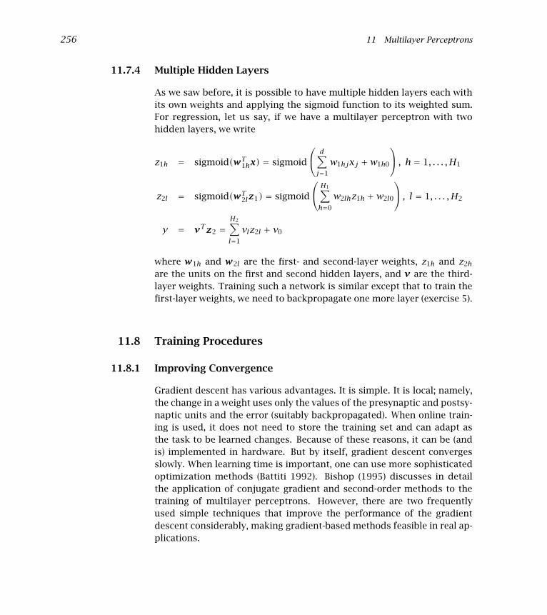
11.7.4 Multiple Hidden Layers
As we saw before, it is possible to have multiple hidden layers each withits own weights and applying the sigmoid function to its weighted sum.For regression, let us say, if we have a multilayer perceptron with twohidden layers, we write
z1h = sigmoid(wT1hx) = sigmoid
⎛
⎝
d∑
j=1
w1hjxj +w1h0
⎞
⎠ , h = 1, . . . ,H1
z2l = sigmoid(wT2lz1) = sigmoid
⎛
⎝
H1∑
h=0
w2lhz1h +w2l0
⎞
⎠ , l = 1, . . . ,H2
y = vTz2 =H2∑
l=1
vlz2l + v0
where w1h and w2l are the first- and second-layer weights, z1h and z2h
are the units on the first and second hidden layers, and v are the third-layer weights. Training such a network is similar except that to train thefirst-layer weights, we need to backpropagate one more layer (exercise 5).
11.8 Training Procedures
11.8.1 Improving Convergence
Gradient descent has various advantages. It is simple. It is local; namely,the change in a weight uses only the values of the presynaptic and postsy-naptic units and the error (suitably backpropagated). When online train-ing is used, it does not need to store the training set and can adapt asthe task to be learned changes. Because of these reasons, it can be (andis) implemented in hardware. But by itself, gradient descent convergesslowly. When learning time is important, one can use more sophisticatedoptimization methods (Battiti 1992). Bishop (1995) discusses in detailthe application of conjugate gradient and second-order methods to thetraining of multilayer perceptrons. However, there are two frequentlyused simple techniques that improve the performance of the gradientdescent considerably, making gradient-based methods feasible in real ap-plications.

11.8 Training Procedures 257
Momentum
Let us say wi is any weight in a multilayer perceptron in any layer, includ-ing the biases. At each parameter update, successive ∆wti values may beso different that large oscillations may occur and slow convergence. t isthe time index that is the epoch number in batch learning and the itera-tion number in online learning. The idea is to take a running average byincorporating the previous update in the current change as if there is amomentum due to previous updates:momentum
∆wti = −η∂Et
∂wi+α∆wt−1
i(11.30)
α is generally taken between 0.5 and 1.0. This approach is especiallyuseful when online learning is used, where as a result we get an effect ofaveraging and smooth the trajectory during convergence. The disadvan-tage is that the past ∆wt−1
i values should be stored in extra memory.
Adaptive Learning Rate
In gradient descent, the learning factor η determines the magnitude ofchange to be made in the parameter. It is generally taken between 0.0and 1.0, mostly less than or equal to 0.2. It can be made adaptive forfaster convergence, where it is kept large when learning takes place andis decreased when learning slows down:
∆η ={
+a if Et+τ < Et
−bη otherwise(11.31)
Thus we increase η by a constant amount if the error on the training setdecreases and decrease it geometrically if it increases. Because E mayoscillate from one epoch to another, it is a better idea to take the averageof the past few epochs as Et .
11.8.2 Overtraining
A multilayer perceptron with d inputs, H hidden units, and K outputshas H(d+1) weights in the first layer and K(H+1) weights in the secondlayer. Both the space and time complexity of an MLP is O(H · (K + d)).When e denotes the number of training epochs, training time complexityis O(e ·H · (K + d)).

258 11 Multilayer Perceptrons
In an application, d and K are predefined and H is the parameter thatwe play with to tune the complexity of the model. We know from pre-vious chapters that an overcomplex model memorizes the noise in thetraining set and does not generalize to the validation set. For example,we have previously seen this phenomenon in the case of polynomial re-gression where we noticed that in the presence of noise or small samples,increasing the polynomial order leads to worse generalization. Similarlyin an MLP, when the number of hidden units is large, the generalizationaccuracy deteriorates (see figure 11.12), and the bias/variance dilemmaalso holds for the MLP, as it does for any statistical estimator (Geman,Bienenstock, and Doursat 1992).
A similar behavior happens when training is continued too long: asmore training epochs are made, the error on the training set decreases,but the error on the validation set starts to increase beyond a certainpoint (see figure 11.13). Remember that initially all the weights are closeto 0 and thus have little effect. As training continues, the most impor-tant weights start moving away from 0 and are utilized. But if training iscontinued further on to get less and less error on the training set, almostall weights are updated away from 0 and effectively become parameters.Thus as training continues, it is as if new parameters are added to the sys-tem, increasing the complexity and leading to poor generalization. Learn-ing should be stopped early to alleviate this problem of overtraining. Theearly stopping
overtraining optimal point to stop training, and the optimal number of hidden units,is determined through cross-validation, which involves testing the net-work’s performance on validation data unseen during training.
Because of the nonlinearity, the error function has many minima andgradient descent converges to the nearest minimum. To be able to assessexpected error, the same network is trained a number of times start-ing from different initial weight values, and the average of the validationerror is computed.
11.8.3 Structuring the Network
In some applications, we may believe that the input has a local structure.For example, in vision we know that nearby pixels are correlated andthere are local features like edges and corners; any object, for example,a handwritten digit, may be defined as a combination of such primitives.Similarly, in speech, locality is in time and inputs close in time can begrouped as speech primitives. By combining these primitives, longer ut-

11.8 Training Procedures 259
0 5 10 15 20 25 300
0.02
0.04
0.06
0.08
0.1
0.12
Number of Hidden Units
Mean
Squ
are E
rror
TrainingValidation
Figure 11.12 As complexity increases, training error is fixed but the validationerror starts to increase and the network starts to overfit.
0 100 200 300 400 500 600 700 800 900 10000
0.5
1
1.5
2
2.5
3
3.5
Training Epochs
Mean
Squ
are E
rror
TrainingValidation
Figure 11.13 As training continues, the validation error starts to increase andthe network starts to overfit.

260 11 Multilayer Perceptrons
Figure 11.14 A structured MLP. Each unit is connected to a local group of unitsbelow it and checks for a particular feature—for example, edge, corner, and soforth—in vision. Only one hidden unit is shown for each region; typically thereare many to check for different local features.
terances, for example, speech phonemes, may be defined. In such a casewhen designing the MLP, hidden units are not connected to all input unitsbecause not all inputs are correlated. Instead, we define hidden units thatdefine a window over the input space and are connected to only a smalllocal subset of the inputs. This decreases the number of connections andtherefore the number of free parameters (Le Cun et al. 1989).
We can repeat this in successive layers where each layer is connectedto a small number of local units below and checks for a more compli-cated feature by combining the features below in a larger part of theinput space until we get to the output layer (see figure 11.14). For ex-ample, the input may be pixels. By looking at pixels, the first hiddenlayer units may learn to check for edges of various orientations. Thenby combining edges, the second hidden layer units can learn to check forcombinations of edges—for example, arcs, corners, line ends—and thencombining them in upper layers, the units can look for semi-circles, rec-tangles, or in the case of a face recognition application, eyes, mouth, andso forth. This is the example of a hierarchical cone where features gethierarchical cone
more complex, abstract, and fewer in number as we go up the networkuntil we get to classes.
In such a case, we can further reduce the number of parameters byweight sharing. Taking the example of visual recognition again, we canweight sharing
see that when we look for features like oriented edges, they may be
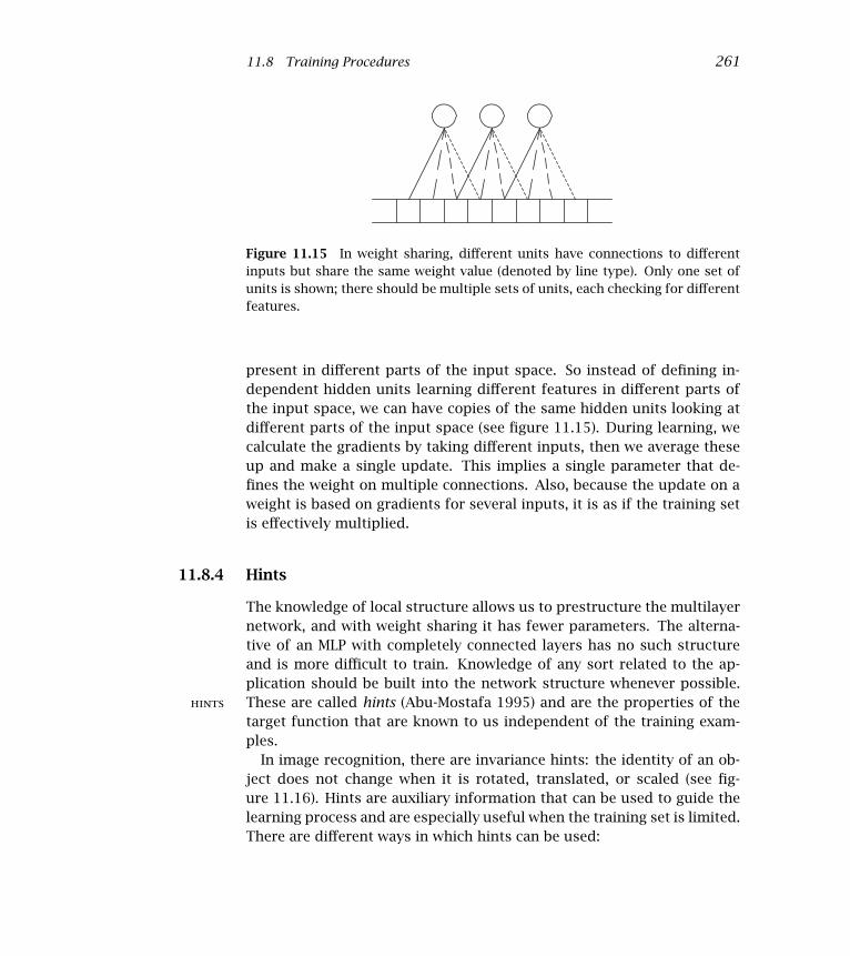
11.8 Training Procedures 261
Figure 11.15 In weight sharing, different units have connections to differentinputs but share the same weight value (denoted by line type). Only one set ofunits is shown; there should be multiple sets of units, each checking for differentfeatures.
present in different parts of the input space. So instead of defining in-dependent hidden units learning different features in different parts ofthe input space, we can have copies of the same hidden units looking atdifferent parts of the input space (see figure 11.15). During learning, wecalculate the gradients by taking different inputs, then we average theseup and make a single update. This implies a single parameter that de-fines the weight on multiple connections. Also, because the update on aweight is based on gradients for several inputs, it is as if the training setis effectively multiplied.
11.8.4 Hints
The knowledge of local structure allows us to prestructure the multilayernetwork, and with weight sharing it has fewer parameters. The alterna-tive of an MLP with completely connected layers has no such structureand is more difficult to train. Knowledge of any sort related to the ap-plication should be built into the network structure whenever possible.These are called hints (Abu-Mostafa 1995) and are the properties of thehints
target function that are known to us independent of the training exam-ples.
In image recognition, there are invariance hints: the identity of an ob-ject does not change when it is rotated, translated, or scaled (see fig-ure 11.16). Hints are auxiliary information that can be used to guide thelearning process and are especially useful when the training set is limited.There are different ways in which hints can be used:

262 11 Multilayer Perceptrons
A A AAFigure 11.16 The identity of the object does not change when it is translated,rotated, or scaled. Note that this may not always be true, or may be true up to apoint: ‘b’ and ‘q’ are rotated versions of each other. These are hints that can beincorporated into the learning process to make learning easier.
1. Hints can be used to create virtual examples. For example, knowingvirtual examples
that the object is invariant to scale, from a given training example,we can generate multiple copies at different scales and add them tothe training set with the same label. This has the advantage that weincrease the training set and do not need to modify the learner in anyway. The problem may be that too many examples may be needed forthe learner to learn the invariance.
2. The invariance may be implemented as a preprocessing stage. Forexample, optical character readers have a preprocessing stage wherethe input character image is centered and normalized for size andslant. This is the easiest solution, when it is possible.
3. The hint may be incorporated into the network structure. Local struc-ture and weight sharing, which we saw in section 11.8.3, is one exam-ple where we get invariance to small translations and rotations.
4. The hint may also be incorporated by modifying the error function. Letus say we know that x and x′ are the same from the application’s pointof view, where x′ may be a “virtual example” of x. That is, f (x) = f (x′),when f (x) is the function we would like to approximate. Let us denoteby g(x|θ), our approximation function, for example, an MLP where θare its weights. Then, for all such pairs (x,x′), we define the penaltyfunction
Eh =[
g(x|θ)− g(x′|θ)]2
and add it as an extra term to the usual error function:
E′ = E + λh · Eh

11.9 Tuning the Network Size 263
This is a penalty term penalizing the cases where our predictions donot obey the hint, and λh is the weight of such a penalty (Abu-Mostafa1995).
Another example is the approximation hint: Let us say that for x, wedo not know the exact value, f (x), but we know that it is in the interval,[ax, bx]. Then our added penalty term is
Eh =
⎧
⎪⎨
⎪⎩
0 if g(x|θ) ∈ [ax, bx](g(x)− ax)2 if g(x|θ) < ax(g(x)− bx)2 if g(x|θ) > bx
This is similar to the error function used in support vector regression(section 13.10), which tolerates small approximation errors.
Still another example is the tangent prop (Simard et al. 1992) wheretangent prop
the transformation against which we are defining the hint—for exam-ple, rotation by an angle—is modeled by a function. The usual errorfunction is modified (by adding another term) so as to allow param-eters to move along this line of transformation without changing theerror.
11.9 Tuning the Network Size
Previously we saw that when the network is too large and has too manyfree parameters, generalization may not be well. To find the optimalnetwork size, the most common approach is to try many different ar-chitectures, train them all on the training set, and choose the one thatgeneralizes best to the validation set. Another approach is to incorporatethis structural adaptation into the learning algorithm. There are two waysstructural
adaptation this can be done:
1. In the destructive approach, we start with a large network and gradu-ally remove units and/or connections that are not necessary.
2. In the constructive approach, we start with a small network and grad-ually add units and/or connections to improve performance.
One destructive method is weight decay where the idea is to remove un-weight decay
necessary connections. Ideally to be able to determine whether a unit orconnection is necessary, we need to train once with and once without and
264 11 Multilayer Perceptrons
check the difference in error on a separate validation set. This is costlysince it should be done for all combinations of such units/connections.
Given that a connection is not used if its weight is 0, we give eachconnection a tendency to decay to 0 so that it disappears unless it isreinforced explicitly to decrease error. For any weight wi in the network,we use the update rule:
∆wi = −η∂E
∂wi− λwi(11.32)
This is equivalent to doing gradient descent on the error function withan added penalty term, penalizing networks with many nonzero weights:
E′ = E + λ
2
∑
i
w2i(11.33)
Simpler networks are better generalizers is a hint that we implement byadding a penalty term. Note that we are not saying that simple networksare always better than large networks; we are saying that if we have twonetworks that have the same training error, the simpler one—namely, theone with fewer weights—has a higher probability of better generalizingto the validation set.
The effect of the second term in equation 11.32 is like that of a springthat pulls each weight to 0. Starting from a value close to 0, unless theactual error gradient is large and causes an update, due to the secondterm, the weight will gradually decay to 0. λ is the parameter that deter-mines the relative importances of the error on the training set and thecomplexity due to nonzero parameters and thus determines the speed ofdecay: With large λ, weights will be pulled to 0 no matter what the train-ing error is; with small λ, there is not much penalty for nonzero weights.λ is fine-tuned using cross-validation.
Instead of starting from a large network and pruning unnecessary con-nections or units, one can start from a small network and add units andassociated connections should the need arise (figure 11.17). In dynamicdynamic node
creation node creation (Ash 1989), an MLP with one hidden layer with one hiddenunit is trained and after convergence, if the error is still high, anotherhidden unit is added. The incoming weights of the newly added unit andits outgoing weight are initialized randomly and trained with the previ-ously existing weights that are not reinitialized and continue from theirprevious values.
In cascade correlation (Fahlman and Lebiere 1990), each added unitcascade
correlation

11.9 Tuning the Network Size 265
Dynamic Node Creation Cascade Correlation
Figure 11.17 Two examples of constructive algorithms. Dynamic node creationadds a unit to an existing layer. Cascade correlation adds each unit as a newhidden layer connected to all the previous layers. Dashed lines denote the newlyadded unit/connections. Bias units/weights are omitted for clarity.
is a new hidden unit in another hidden layer. Every hidden layer hasonly one unit that is connected to all of the hidden units preceding itand the inputs. The previously existing weights are frozen and are nottrained; only the incoming and outgoing weights of the newly added unitare trained.
Dynamic node creation adds a new hidden unit to an existing hiddenlayer and never adds another hidden layer. Cascade correlation alwaysadds a new hidden layer with a single unit. The ideal constructive methodshould be able to decide when to introduce a new hidden layer and whento add a unit to an existing layer. This is an open research problem.
Incremental algorithms are interesting because they correspond to mod-ifying not only the parameters but also the model structure during learn-ing. We can think of a space defined by the structure of the multilayerperceptron and operators corresponding to adding/removing unit(s) orlayer(s) to move in this space (Aran et al. 2009). Incremental algorithmsthen do a search in this state space where operators are tried (accordingto some order) and accepted or rejected depending on some goodnessmeasure, for example, some combination of complexity and validation er-ror. Another example would be a setting in polynomial regression where

266 11 Multilayer Perceptrons
high-order terms are added/removed during training automatically, fit-ting model complexity to data complexity. As the cost of computationgets lower, such automatic model selection should be a part of the learn-ing process done automatically without any user interference.
11.10 Bayesian View of Learning
The Bayesian approach in training neural networks considers the param-eters, namely, connection weights, wi , as random variables drawn froma prior distribution p(wi) and computes the posterior probability giventhe data
p(w|X) = p(X|w)p(w)p(X)(11.34)
where w is the vector of all weights of the network. The MAP estimate wis the mode of the posterior
wMAP = arg maxw
logp(w|X)(11.35)
Taking the log of equation 11.34, we get
logp(w|X) = logp(X|w)+ logp(w)+ C
The first term on the right is the log likelihood, and the second is thelog of the prior. If the weights are independent and the prior is taken asGaussian, N (0,1/2λ)
p(w) =∏
i
p(wi) where p(wi) = c · exp
[
− w2i
2(1/2λ)
]
(11.36)
the MAP estimate minimizes the augmented error function
E′ = E + λ∥w∥2(11.37)
where E is the usual classification or regression error (negative log like-lihood). This augmented error is exactly the error function we used inweight decay (equation 11.33). Using a large λ assumes small variabilityin parameters, puts a larger force on them to be close to 0, and takesthe prior more into account than the data; if λ is small, then the allowedvariability of the parameters is larger. This approach of removing unnec-essary parameters is known as ridge regression in statistics.ridge regression
This is another example of regularization with a cost function, combin-regularization

11.11 Dimensionality Reduction 267
ing the fit to data and model complexity
cost = data-misfit+ λ · complexity(11.38)
The use of Bayesian estimation in training multilayer perceptrons istreated in MacKay 1992a, b. We are going to talk about Bayesian estima-tion in more detail in chapter 14.
Empirically, it has been seen that after training, most of the weightsof a multilayer perceptron are distributed normally around 0, justifyingthe use of weight decay. But this may not always be the case. Nowlanand Hinton (1992) proposed soft weight sharing where weights are drawnsoft weight sharing
from a mixture of Gaussians, allowing them to form multiple clusters, notone. Also, these clusters may be centered anywhere and not necessarilyat 0, and have variances that are modifiable. This changes the prior ofequation 11.36 to a mixture of M ≥ 2 Gaussians
p(wi) =M∑
j=1
αjpj(wi)(11.39)
whereαj are the priors and pj(wi) ∼N (mj, s2j ) are the component Gaus-
sians. M is set by the user and αj ,mj, sj are learned from the data.Using such a prior and augmenting the error function with its log dur-ing training, the weights converge to decrease error and also are groupedautomatically to increase the log prior.
11.11 Dimensionality Reduction
In a multilayer perceptron, if the number of hidden units is less than thenumber of inputs, the first layer performs a dimensionality reduction.The form of this reduction and the new space spanned by the hiddenunits depend on what the MLP is trained for. If the MLP is for classifica-tion with output units following the hidden layer, then the new space isdefined and the mapping is learned to minimize classification error (seefigure 11.18).
We can get an idea of what the MLP is doing by analyzing the weights.We know that the dot product is maximum when the two vectors areidentical. So we can think of each hidden unit as defining a template inits incoming weights, and by analyzing these templates, we can extractknowledge from a trained MLP. If the inputs are normalized, weights tellus of their relative importance. Such analysis is not easy but gives us

268 11 Multilayer Perceptrons
0 0.1 0.2 0.3 0.4 0.5 0.6 0.7 0.8 0.9 10
0.1
0.2
0.3
0.4
0.5
0.6
0.7
0.8
0.9
1
Hidden 1
Hidd
en 2
Hidden Representation
00
7
4
62
5
5
0
8
7
19
5
3
0
4
7
8
47
8
5
9
1
2
0
6
1
8
7
0
7
6
9 1
9
3
9 4
9
2
1
99
6
4
3
2
8
2
71 4
62 0
4
6
3
7
1
022
5
2
4
8
1
7
3
0
33
77
9
1
3
3
4
3
4
2
88
9
8
4
7
1
6
94
0
1
3
6
2
Figure 11.18 Optdigits data plotted in the space of the two hidden units ofan MLP trained for classification. Only the labels of one hundred data points areshown. This MLP with sixty-four inputs, two hidden units, and ten outputs has 80percent accuracy. Because of the sigmoid, hidden unit values are between 0 and1 and classes are clustered around the corners. This plot can be compared withthe plots in chapter 6, which are drawn using other dimensionality reductionmethods on the same dataset.
some insight as to what the MLP is doing and allows us to peek into theblack box.
An interesting architecture is the autoassociator (Cottrell, Munro, andautoassociator
Zipser 1987), which is an MLP architecture where there are as many out-puts as there are inputs, and the required outputs are defined to be equalto the inputs (see figure 11.19). To be able to reproduce the inputs againat the output layer, the MLP is forced to find the best representation ofthe inputs in the hidden layer. When the number of hidden units is lessthan the number of inputs, this implies dimensionality reduction. Once

11.11 Dimensionality Reduction 269
x0=+1 x1 xd
zH
Encoder
y1 yd
Decoder
y1 yd
x0=+1 x1 xd
zH
Linear Nonlinear
Figure 11.19 In the autoassociator, there are as many outputs as there areinputs and the desired outputs are the inputs. When the number of hidden unitsis less than the number of inputs, the MLP is trained to find the best coding ofthe inputs on the hidden units, performing dimensionality reduction. On theleft, the first layer acts as an encoder and the second layer acts as the decoder.On the right, if the encoder and decoder are multilayer perceptrons with sigmoidhidden units, the network performs nonlinear dimensionality reduction.
the training is done, the first layer from the input to the hidden layeracts as an encoder, and the values of the hidden units make up the en-coded representation. The second layer from the hidden units to theoutput units acts as a decoder, reconstructing the original signal from itsencoded representation.
It has been shown (Bourlard and Kamp 1988) that an MLP with onehidden layer of units implements principal components analysis (sec-tion 6.3), except that the hidden unit weights are not the eigenvectorssorted in importance using the eigenvalues but span the same space astheH principal eigenvectors. If the encoder and decoder are not one layerbut multilayer perceptrons with sigmoid nonlinearity in the hidden units,the encoder implements nonlinear dimensionality reduction (Hinton andSalakhutdinov 2006).
Another way to use an MLP for dimensionality reduction is throughmultidimensional scaling (section 6.5). Mao and Jain (1995) show how anMLP can be used to learn the Sammon mapping. Recalling equation 6.29,Sammon mapping
270 11 Multilayer Perceptrons
Sammon stress is defined as
E(θ|X) =∑
r ,s
[∥g(xr |θ)− g(xs|θ)∥ − ∥xr − xs∥∥xr − xs∥
]2
(11.40)
An MLP with d inputs,H hidden units, and k < d output units is used toimplement g(x|θ), mapping the d-dimensional input to a k-dimensionalvector, where θ corresponds to the weights of the MLP. Given a dataset ofX = {xt}t , we can use gradient descent to minimize the Sammon stressdirectly to learn the MLP, namely, g(x|θ), such that the distances be-tween the k-dimensional representations are as close as possible to thedistances in the original space.
11.12 Learning Time
Until now, we have been concerned with cases where the input is fedonce, all together. In some applications, the input is temporal where weneed to learn a temporal sequence. In others, the output may also changein time. Examples are as follows:
! Sequence recognition. This is the assignment of a given sequence toone of several classes. Speech recognition is one example where theinput signal sequence is the spoken speech and the output is the codeof the word spoken. That is, the input changes in time but the outputdoes not.
! Sequence reproduction. Here, after seeing part of a given sequence, thesystem should predict the rest. Time-series prediction is one examplewhere the input is given but the output changes.
! Temporal association. This is the most general case where a particularoutput sequence is given as output after a specific input sequence. Theinput and output sequences may be different. Here both the input andthe output change in time.
11.12.1 Time Delay Neural Networks
The easiest way to recognize a temporal sequence is by converting it to aspatial sequence. Then any method discussed up to this point can be uti-lized for classification. In a time delay neural network (Waibel et al. 1989),time delay neural
network

11.12 Learning Time 271
Figure 11.20 A time delay neural network. Inputs in a time window of length Tare delayed in time until we can feed all T inputs as the input vector to the MLP.
previous inputs are delayed in time so as to synchronize with the final in-put, and all are fed together as input to the system (see figure 11.20).Backpropagation can then be used to train the weights. To extract fea-tures local in time, one can have layers of structured connections andweight sharing to get translation invariance in time. The main restrictionof this architecture is that the size of the time window we slide over thesequence should be fixed a priori.
11.12.2 Recurrent Networks
In a recurrent network, additional to the feedforward connections, unitsrecurrent network
have self-connections or connections to units in the previous layers. Thisrecurrency acts as a short-term memory and lets the network rememberwhat happened in the past.
Most frequently, one uses a partially recurrent network where a lim-ited number of recurrent connections are added to a multilayer percep-tron (see figure 11.21). This combines the advantage of the nonlinearapproximation ability of a multilayer perceptron with the temporal rep-resentation ability of the recurrency, and such a network can be used toimplement any of the three temporal association tasks. It is also possibleto have hidden units in the recurrent backward connections, these being

272 11 Multilayer Perceptrons
(a) (c)(b)
Figure 11.21 Examples of MLP with partial recurrency. Recurrent connectionsare shown with dashed lines: (a) self-connections in the hidden layer, (b) self-connections in the output layer, and (c) connections from the output to thehidden layer. Combinations of these are also possible.
known as context units. No formal results are known to determine howto choose the best architecture given a particular application.
If the sequences have a small maximum length, then unfolding in timeunfolding in time
can be used to convert an arbitrary recurrent network to an equivalentfeedforward network (see figure 11.22). A separate unit and connectionis created for copies at different times. The resulting network can betrained with backpropagation with the additional requirement that allcopies of each connection should remain identical. The solution, as inweight sharing, is to sum up the different weight changes in time andchange the weight by the average. This is called backpropagation throughbackpropagation
through time time (Rumelhart, Hinton, and Willams 1986b). The problem with this ap-proach is the memory requirement if the length of the sequence is large.Real time recurrent learning (Williams and Zipser 1989) is an algorithmreal time recurrent
learning for training recurrent networks without unfolding and has the advantagethat it can use sequences of arbitrary length.
11.13 Notes
Research on artificial neural networks is as old as the digital computer.McCulloch and Pitts (1943) proposed the first mathematical model for theartificial neuron. Rosenblatt (1962) proposed the perceptron model and alearning algorithm in 1962. Minsky and Papert (1969) showed the limita-

11.13 Notes 273
(a) (b)x
x3
x0
x1
x2
W
y
h
VR
W
W
W
W R
R
R
V
h0
h3
h1
h2
y
Figure 11.22 Backpropagation through time: (a) recurrent network, and (b) itsequivalent unfolded network that behaves identically in four steps.
tion of single-layer perceptrons, for example, the XOR problem, and sincethere was no algorithm to train a multilayer perceptron with a hiddenlayer at that time, the work on artificial neural networks almost stoppedexcept at a few places. The renaissance of neural networks came withthe paper by Hopfield (1982). This was followed by the two-volume Paral-lel Distributed Processing (PDP) book written by the PDP Research Group(Rumelhart, McClelland, and the PDP Research Group 1986). It seems asthough backpropagation was invented independently in several places al-most at the same time and the limitation of a single-layer perceptron nolonger held.
Starting in the mid-1980s, there has been a huge explosion of work onartificial neural network models from various disciplines: physics, statis-tics, psychology, cognitive science, neuroscience, and lingustics, not tomention computer science, electrical engineering, and adaptive control.

274 11 Multilayer Perceptrons
Perhaps the most important contribution of research on artificial neu-ral networks is this synergy that bridged various disciplines, especiallystatistics and engineering. It is thanks to this that the field of machinelearning is now well established.
The field is much more mature now; aims are more modest and betterdefined. One of the criticisms of backpropagation was that it was notbiologically plausible! Though the term “neural network” is still widelyused, it is generally understood that neural network models, for example,multilayer perceptrons, are nonparametric estimators and that the bestway to analyze them is by using statistical methods.
For example, a statistical method similar to the multilayer perceptronis projection pursuit (Friedman and Stuetzle 1981), which is written asprojection pursuit
y =H∑
h=1
φh(wThx)
the difference being that each “hidden unit” has its own separate func-tion, φh(·), though in an MLP, all are fixed to be sigmoid. In chapter 12,we will see another neural network structure, named radial basis func-tions, which uses the Gaussian function at the hidden units.
There are various textbooks on artificial neural networks: Hertz, Krogh,and Palmer 1991, the earliest, is still readable. Bishop 1995 has a patternrecognition emphasis and discusses in detail various optimization algo-rithms that can be used for training, as well as the Bayesian approach,generalizing weight decay. Ripley 1996 analyzes neural networks from astatistical perspective.
Artificial neural networks, for example, multilayer perceptrons, havevarious successful applications. In addition to their various successfulapplications in adaptive control, speech recognition, and vision, two arenoteworthy: Tesauro’s TD-Gammon program (Tesauro 1994) uses rein-forcement learning (chapter 18) to train a multilayer perceptron and playsbackgammon at a master level. Pomerleau’s ALVINN is a neural networkthat autonomously drives a van up to 20 miles per hour after learning byobserving a driver for five minutes (Pomerleau 1991).
11.14 Exercises
1. Show the perceptron that calculates NOT of its input.
2. Show the perceptron that calculates NAND of its two inputs.

11.15 References 275
3. Show the perceptron that calculates the parity of its three inputs.
4. Derive the update equations when the hidden units use tanh, instead of thesigmoid. Use the fact that tanh′ = (1− tanh2).
5. Derive the update equations for an MLP with two hidden layers.
6. Consider a MLP architecture with one hidden layer where there are also directweights from the inputs directly to the output units. Explain when such astructure would be helpful and how it can be trained.
7. Parity is cyclic shift invariant; for example, “0101” and “1010” have the sameparity. Propose a multilayer perceptron to learn the parity function using thishint.
8. In cascade correlation, what are the advantages of freezing the previouslyexisting weights?
9. Derive the update equations for an MLP implementing Sammon mapping thatminimizes Sammon stress (equation 11.40).
10. In section 11.6, we discuss how a MLP with two hidden layers can implementpiecewise constant approximation. Show that if the weight in the last layer isnot a constant but a linear function of the input, we can implement piecewiselinear approximation.
11. Derive the update equations for soft weight sharing.
12. In the autoassociator network, how can we decide on the number of hiddenunits?
13. Incremental learning of the structure of a MLP can be viewed as a state spacesearch. What are the operators? What is the goodness function? What type ofsearch strategies are appropriate? Define these in such a way that dynamicnode creation and cascade-correlation are special instantiations.
14. For the MLP given in figure 11.22, derive the update equations for the un-folded network.
11.15 References
Abu-Mostafa, Y. 1995. “Hints.” Neural Computation 7: 639–671.
Aran, O., O. T. Yıldız, and E. Alpaydın. 2009. “An Incremental Framework Basedon Cross-Validation for Estimating the Architecture of a Multilayer Percep-tron.” International Journal of Pattern Recognition and Artificial Intelligence
23: 159–190.
Ash, T. 1989. “Dynamic Node Creation in Backpropagation Networks.” Connec-
tion Science 1: 365–375.

276 11 Multilayer Perceptrons
Battiti, R. 1992. “First- and Second-Order Methods for Learning: Between Steep-est Descent and Newton’s Method.” Neural Computation 4: 141–166.
Bishop, C. M. 1995. Neural Networks for Pattern Recognition. Oxford: OxfordUniversity Press.
Bourlard, H., and Y. Kamp. 1988. “Auto-Association by Multilayer Perceptronsand Singular Value Decomposition.” Biological Cybernetics 59: 291–294.
Cottrell, G. W., P. Munro, and D. Zipser. 1987. “Learning Internal Representa-tions from Gray-Scale Images: An Example of Extensional Programming.” InNinth Annual Conference of the Cognitive Science Society, 462–473. Hillsdale,NJ: Erlbaum.
Durbin, R., and D. E. Rumelhart. 1989. “Product Units: A ComputationallyPowerful and Biologically Plausible Extension to Backpropagation Networks.”Neural Computation 1: 133–142.
Fahlman, S. E., and C. Lebiere. 1990. “The Cascade Correlation Architecture.”In Advances in Neural Information Processing Systems 2, ed. D. S. Touretzky,524–532. San Francisco: Morgan Kaufmann.
Friedman, J. H., and W. Stuetzle. 1981. “Projection Pursuit Regression.” Journal
of the American Statistical Association 76: 817–823.
Geman, S., E. Bienenstock, and R. Doursat. 1992. “Neural Networks and theBias/Variance Dilemma.” Neural Computation 4: 1–58.
Hertz, J., A. Krogh, and R. G. Palmer. 1991. Introduction to the Theory of Neural
Computation. Reading, MA: Addison Wesley.
Hinton, G. E., and R. R. Salakhutdinov. 2006. “Reducing the dimensionality ofdata with neural networks.” Science 313: 504–507.
Hopfield, J. J. 1982. “Neural Networks and Physical Systems with EmergentCollective Computational Abilities.” Proceedings of the National Academy of
Sciences USA 79: 2554–2558.
Hornik, K., M. Stinchcombe, and H. White. 1989. “Multilayer Feedforward Net-works Are Universal Approximators.” Neural Networks 2: 359–366.
Le Cun, Y., B. Boser, J. S. Denker, D. Henderson, R. E. Howard, W. Hubbard,and L. D. Jackel. 1989. “Backpropagation Applied to Handwritten ZipcodeRecognition.” Neural Computation 1: 541–551.
MacKay, D. J. C. 1992a. “Bayesian Interpolation.” Neural Computation 4: 415–447.
MacKay, D. J. C. 1992b. “A Practical Bayesian Framework for BackpropagationNetworks” Neural Computation 4: 448–472.
Mao, J., and A. K. Jain. 1995. “Artificial Neural Networks for Feature Extractionand Multivariate Data Projection.” IEEE Transactions on Neural Networks 6:296–317.

11.15 References 277
Marr, D. 1982. Vision. New York: Freeman.
McCulloch, W. S., and W. Pitts. 1943. “A Logical Calculus of the Ideas Immenentin Nervous Activity.” Bulletin of Mathematical Biophysics 5: 115–133.
Minsky, M. L., and S. A. Papert. 1969. Perceptrons. Cambridge, MA: MIT Press.(Expanded ed. 1990.)
Nowlan, S. J., and G. E. Hinton. 1992. “Simplifying Neural Networks by SoftWeight Sharing.” Neural Computation 4: 473–493.
Pomerleau, D. A. 1991. “Efficient Training of Artificial Neural Networks forAutonomous Navigation.” Neural Computation 3: 88–97.
Posner, M. I., ed. 1989. Foundations of Cognitive Science. Cambridge, MA: MITPress.
Richard, M. D., and R. P. Lippmann. 1991. “Neural Network Classifiers EstimateBayesian a Posteriori Probabilities.” Neural Computation 3: 461–483.
Ripley, B. D. 1996. Pattern Recognition and Neural Networks. Cambridge, UK:Cambridge University Press.
Rosenblatt, F. 1962. Principles of Neurodynamics: Perceptrons and the Theory
of Brain Mechanisms. New York: Spartan.
Rumelhart, D. E., G. E. Hinton, and R. J. Williams. 1986a. “Learning Representa-tions by Backpropagating Errors.” Nature 323: 533–536.
Rumelhart, D. E., G. E. Hinton, and R. J. Williams. 1986b. “Learning InternalRepresentations by Error Propagation.” In Parallel Distributed Processing, ed.D. E. Rumelhart, J. L. McClelland, and the PDP Research Group, 318–362. Cam-bridge, MA: MIT Press.
Rumelhart, D. E., J. L. McClelland, and the PDP Research Group, eds. 1986.Parallel Distributed Processing. Cambridge, MA: MIT Press.
Simard, P., B. Victorri, Y, Le Cun, and J. Denker. 1992. “Tangent Prop: A Formal-ism for Specifying Selected Invariances in an Adaptive Network.” In Advances
in Neural Information Processing Systems 4, ed. J. E. Moody, S. J. Hanson, andR. P. Lippman, 895–903. San Francisco: Morgan Kaufmann.
Tesauro, G. 1994. “TD-Gammon, A Self-Teaching Backgammon Program, AchievesMaster-Level Play.” Neural Computation 6: 215–219.
Thagard, P. 2005. Mind: Introduction to Cognitive Science. 2nd ed. Cambridge,MA: MIT Press.
Waibel, A., T. Hanazawa, G. Hinton, K. Shikano, and K. Lang. 1989. “PhonemeRecognition Using Time-Delay Neural Networks.” IEEE Transactions on Acous-
tics, Speech, and Signal Processing 37: 328–339.
Williams, R. J., and D. Zipser. 1989. “A Learning Algorithm for ContinuallyRunning Fully Recurrent Neural Networks.” Neural Computation 1: 270–280.