Introduction to MathematicaME305 & AM501 1993 Winter

Noboru Kikuchi

Matrix and Vector Algebra

define a 3-by-4 matrix A

After defining a 3-by-4 matrix A, we output it in the form of a matrix. In Mathematica, 1,2,3,... are recognized as symbols rather than numerical values. We shall recognize this feature in the following operation.

A={{1,2,3,4},{5,4,7,8},{-4,-3,-2,-1}};MatrixForm[A]

1 2 3 45 4 7 8-4 -3 -2 -1

find the eigenvalues of a square matrix AAT

We shall compute the eigenvalues of a square matrix obtained by AAT. To this end, there are

two ways to do it. The first is computation of the eigenvalues numerically by defining the matrix numericall using the operation N[ ]. If we do not operate N[ ] on the square matrix, its components are recognized as symbols, and then it takes considerably large amount of algebra to find the eigenvalues without introducing any of "round off or approximation" errors. It is noted that we can compute the eigenvalues for symbols after large compution, but it is not realistic at all.

Eigenvalues[N[A.Transpose[A]]]Eigenvalues[A.Transpose[A]]

{201.805, 0.598203, 11.5971}

5/3 214 4799 2{--- + ---------------------------------- + -- --------------------------------- 3 1/3 3 (465160 + I Sqrt[4671963198]) 4/3 1/3 2 (465160 + I Sqrt[4671963198]) -------------------------------------, ------------------------------------ 3 5/3 214 I -4799 2 --- + - Sqrt[3] (---------------------------------- + -- --------------------------------- 3 2 1/3 3 (465160 + I Sqrt[4671963198]) 4/3 1/3 2 (465160 + I Sqrt[4671963198]) -------------------------------------) - ------------------------------------ 3 5/3 4799 2 (---------------------------------- + --------------------------------- 1/3 3 (465160 + I Sqrt[4671963198]) 4/3 1/3 2 (465160 + I Sqrt[4671963198]) -------------------------------------) / 2, ------------------------------------ 3 5/3 214 I -4799 2 --- - - Sqrt[3] (---------------------------------- + -- --------------------------------- 3 2 1/3 3 (465160 + I Sqrt[4671963198]) 4/3 1/3 2 (465160 + I Sqrt[4671963198]) -------------------------------------) - ------------------------------------ 3 5/3 4799 2 (---------------------------------- + --------------------------------- 1/3 3 (465160 + I Sqrt[4671963198]) 4/3 1/3 2 (465160 + I Sqrt[4671963198]) -------------------------------------) / 2} ------------------------------------ 3

It is certain that not only the eigenvalues but also the eigenvectors of a square matrix can be obtained numerically in Mathematica. Further, if we wish to compute both the eigenvalues and eigenvectors, it can be done by using command Eigensystem[ ] rather than Eigenvalues[ ] and Eigenvectors[ ].

Eigenvectors[N[A.Transpose[A]]]Eigensystem[N[A.Transpose[A]]]

{{0.372034, 0.872243, -0.317464}, {-0.848767, 0.458123, 0.264041}, {-0.375745, -0.17122, -0.910768}}

{{201.805, 0.598203, 11.5971}, {{0.372034, 0.872243, -0.317464}, {-0.848767, 0.458123, 0.264041}, {-0.375745, -0.17122, -0.910768}}}

IntroMATH 2

A Complex Matrix

Using two 3-by-3 matrices A and B, we shall describe a complex matrix AB. "I" in Mathematica means Sqrt[-1] for expression of complex numbers. We can extract the real and imaginary portions from general complex numbers/matrices using Re[ ] and Im[ ], respectively. Furthermore, the absolute value and argument of each complex component of a matrix can also be computed in Mathematica using Abs[ ] and Arg[ ] operations, respectively. "%" is identified with the variable obtained ( or defined ) in the last operation in Mathematica,and g//N means that g will be regarded as numbers rather than symbols.

A={{1,2,3},{3,2,1},{-1,1,-1}}B={{1,0,1},{-1,-1,1},{4,1,2}}AB=A + I B;MatrixForm[AB]MatrixForm[Re[AB]]MatrixForm[Im[AB]]Abs[AB]MatrixForm[%//N]Arg[AB]MatrixForm[%//N]

{{1, 2, 3}, {3, 2, 1}, {-1, 1, -1}}

{{1, 0, 1}, {-1, -1, 1}, {4, 1, 2}}

1 + I 2 3 + I3 - I 2 - I 1 + I-1 + 4 I 1 + I -1 + 2 I

1 2 33 2 1-1 1 -1

1 0 1-1 -1 14 1 2

{{Sqrt[2], 2, Sqrt[10]}, {Sqrt[10], Sqrt[5], Sqrt[2]}, {Sqrt[17], Sqrt[2], Sqrt[5]}}

1.41421 2. 3.162283.16228 2.23607 1.414214.12311 1.41421 2.23607

Pi Pi{{--, 0, ArcTan[3, 1]}, {ArcTan[3, -1], ArcTan[2, -1], --}, - - 4 4 Pi {ArcTan[-1, 4], --, ArcTan[-1, 2]}} - 4

0.785398 0 0.321751-0.321751 -0.463648 0.7853981.81577 0.785398 2.03444

IntroMATH 3

Vector Algebra

Two three components vectors u and v are defined, then we operate "*", "/", ".", and Outer[Times,u,v]. "*" and "/" are operated to each component, while "." means the inner (

scalar ) product uTv of two vectors. Outer[Times, u, v] means that uvT.

u={u1,u2,u3}v={v1,v2,v3}u*vu/vu.vOuter[Times,u,v]

{u1, u2, u3}

{v1, v2, v3}

{u1 v1, u2 v2, u3 v3}

u1 u2 u3{--, --, --} - - - v1 v2 v3

u1 v1 + u2 v2 + u3 v3

{{u1 v1, u1 v2, u1 v3}, {u2 v1, u2 v2, u2 v3}, {u3 v1, u3 v2, u3 v3}}

Matrix Albegra

After defining two 3-by-3 matrices A and B symbolically, we make algebra "+", "*", "/", "^" and "." in Mathematica. It follows from the output that these operations are applied on each component except "." that assumes matrix multiplication instead of componentwise multiplication.

Transpose[A] means AT. Det[A] is the determinant of a square matrix A, while Inverse[A] is A-

1. In this example, we define the inverse of A by a new matrix AI.

A={{a11,a12,a13},{a21,a22,a23},{a31,a32,a33}};MatrixForm[A]B={{b11,b12,b13},{b21,b22,b23},{b31,b32,b33}};MatrixForm[B]A+BA*BA/BA.BTranspose[A]A^2A^(-1)Det[A]AI=Inverse[A]

IntroMATH 4

a11 a12 a13a21 a22 a23a31 a32 a33

b11 b12 b13b21 b22 b23b31 b32 b33

{{a11 + b11, a12 + b12, a13 + b13}, {a21 + b21, a22 + b22, a23 + b23}, {a31 + b31, a32 + b32, a33 + b33}}

{{a11 b11, a12 b12, a13 b13}, {a21 b21, a22 b22, a23 b23}, {a31 b31, a32 b32, a33 b33}}

a11 a12 a13 a21 a22 a23 a31 a32 a33{{---, ---, ---}, {---, ---, ---}, {---, ---, ---}} -- -- -- -- -- -- -- -- -- b11 b12 b13 b21 b22 b23 b31 b32 b33

{{a11 b11 + a12 b21 + a13 b31, a11 b12 + a12 b22 + a13 b32, a11 b13 + a12 b23 + a13 b33}, {a21 b11 + a22 b21 + a23 b31, a21 b12 + a22 b22 + a23 b32, a21 b13 + a22 b23 + a23 b33} , {a31 b11 + a32 b21 + a33 b31, a31 b12 + a32 b22 + a33 b32, a31 b13 + a32 b23 + a33 b33} }

{{a11, a21, a31}, {a12, a22, a32}, {a13, a23, a33}}

2 2 2 2 2 2 2 2 2{{a11 , a12 , a13 }, {a21 , a22 , a23 }, {a31 , a32 , a33 }}

1 1 1 1 1 1 1 1 1{{---, ---, ---}, {---, ---, ---}, {---, ---, ---}} -- -- -- -- -- -- -- -- -- a11 a12 a13 a21 a22 a23 a31 a32 a33

-(a13 a22 a31) + a12 a23 a31 + a13 a21 a32 - a11 a23 a32 - a12 a21 a33 + a11 a22 a33

IntroMATH 5

{{(-(a23 a32) + a22 a33) / (-(a13 a22 a31) + a12 a23 a31 + a13 a21 a32 - a11 a23 a32 - a12 a21 a33 + a11 a22 a33), (a13 a32 - a12 a33) / (-(a13 a22 a31) + a12 a23 a31 + a13 a21 a32 - a11 a23 a32 - a12 a21 a33 + a11 a22 a33), (-(a13 a22) + a12 a23) / (-(a13 a22 a31) + a12 a23 a31 + a13 a21 a32 - a11 a23 a32 - a12 a21 a33 + a11 a22 a33)}, {(a23 a31 - a21 a33) / (-(a13 a22 a31) + a12 a23 a31 + a13 a21 a32 - a11 a23 a32 - a12 a21 a33 + a11 a22 a33), (-(a13 a31) + a11 a33) / (-(a13 a22 a31) + a12 a23 a31 + a13 a21 a32 - a11 a23 a32 - a12 a21 a33 + a11 a22 a33), (a13 a21 - a11 a23) / (-(a13 a22 a31) + a12 a23 a31 + a13 a21 a32 - a11 a23 a32 - a12 a21 a33 + a11 a22 a33)}, {(-(a22 a31) + a21 a32) / (-(a13 a22 a31) + a12 a23 a31 + a13 a21 a32 - a11 a23 a32 - a12 a21 a33 + a11 a22 a33), (a12 a31 - a11 a32) / (-(a13 a22 a31) + a12 a23 a31 + a13 a21 a32 - a11 a23 a32 - a12 a21 a33 + a11 a22 a33), (-(a12 a21) + a11 a22) / (-(a13 a22 a31) + a12 a23 a31 + a13 a21 a32 - a11 a23 a32 - a12 a21 a33 + a11 a22 a33)}}

If components of a matrix are rational functions, then we can pick up only their denominator or/and numerator. Indeed, in Mathematica

IntroMATH 6

Denominator[AI]Numerator[AI]

{{-(a13 a22 a31) + a12 a23 a31 + a13 a21 a32 - a11 a23 a32 - a12 a21 a33 + a11 a22 a33, -(a13 a22 a31) + a12 a23 a31 + a13 a21 a32 - a11 a23 a32 - a12 a21 a33 + a11 a22 a33, -(a13 a22 a31) + a12 a23 a31 + a13 a21 a32 - a11 a23 a32 - a12 a21 a33 + a11 a22 a33}, {-(a13 a22 a31) + a12 a23 a31 + a13 a21 a32 - a11 a23 a32 - a12 a21 a33 + a11 a22 a33, -(a13 a22 a31) + a12 a23 a31 + a13 a21 a32 - a11 a23 a32 - a12 a21 a33 + a11 a22 a33, -(a13 a22 a31) + a12 a23 a31 + a13 a21 a32 - a11 a23 a32 - a12 a21 a33 + a11 a22 a33}, {-(a13 a22 a31) + a12 a23 a31 + a13 a21 a32 - a11 a23 a32 - a12 a21 a33 + a11 a22 a33, -(a13 a22 a31) + a12 a23 a31 + a13 a21 a32 - a11 a23 a32 - a12 a21 a33 + a11 a22 a33, -(a13 a22 a31) + a12 a23 a31 + a13 a21 a32 - a11 a23 a32 - a12 a21 a33 + a11 a22 a33}}

{{-(a23 a32) + a22 a33, a13 a32 - a12 a33, -(a13 a22) + a12 a23}, {a23 a31 - a21 a33, -(a13 a31) + a11 a33, a13 a21 - a11 a23}, {-(a22 a31) + a21 a32, a12 a31 - a11 a32, -(a12 a21) + a11 a22}}

Solution of Algebraic Equations

We can solve a system of linear ( or even nonlinear ) equations symbolically in Mathematica y using Solve command. If a single equation is considered, we can express it as a single equation. If several equations must be considered, then these should be expressed in a form of list ( i.e. vector ) in Mathematica. After setting up equations, we must specify the variables we would like to find. In the following examples, we have two equations, and they are solved for x1 and x2.

Solve[{a11*x1+a12*x2==b1, a21*x1+a22*x2==b2}, {x1,x2}]

{{x1 -> -( -((-(a12 a21) + a11 a22) b1) - a12 (a21 b1 - a11 b2) ----------------------------------------------------)\ --------------------------------------------------- a11 (-(a12 a21) + a11 a22) a21 b1 - a11 b2 , x2 -> -(--------------------)}} ------------------- -(a12 a21) + a11 a22

IntroMATH 7

Functions and Their Graphical Representation

Definition of a Function

We shall look at capability of Mathematica for function operations and graphic capability. First two functions f and g are defined so that we can substitute any expression to the argument.

f[x_]:=x-2 x+x^2 + x Cos[Exp[-x]]g[y_]:=y+y^2 Sin[1/(1+y^2)]

Operation of a Function

Using these two functions, we shall define a new function f(xy)+g(x+y) that is a function of x and y. Then we shall express this function as a polynomial of x whose coefficients are functions of y by using Collect[h,x] command in Mathematica. The same function is also collected in y instead of x.

Collect[f[x y] + g[x+y],x]Collect[f[x y] + g[x+y],y]Coefficient[f[x y] + g[x+y],x^2]

2 1 2 2 1y + y Sin[------------] + x (y + Sin[------------]) + ----------- ----------- 2 2 1 + (x + y) 1 + (x + y) -(x y) 1 x (1 - y + y Cos[E ] + 2 y Sin[------------]) ----------- 2 1 + (x + y)

2 1 2 2 1x + x Sin[------------] + y (x + Sin[------------]) + ----------- ----------- 2 2 1 + (x + y) 1 + (x + y) -(x y) 1 y (1 - x + x Cos[E ] + 2 x Sin[------------]) ----------- 2 1 + (x + y)

2y

IntroMATH 8

Graphics

The functions f and g are defined in arbitrary arguments x and y by adding _ after x and y, we can define functions in other variable, say z. We shall plot the functions f(z) and g(z) in the interval (-4,4) using Plot command. The third command ParametricPlot draws a curve defined on the two dimensional plane with a parameter x in (-4,4). A new function fg is then defined by f(pq)g(1+p-q) that is a function of p and q. The profile of this function is plotted on the domain (-2,2)x(-2,2). "PlotRange -> All" in Plot command means that the whole profile of the function is plotted without trancation of the function. "PlotPoints -> 20" in Plot command means that 20 subintervals are assumed in each direction to define the profile. If this number is increased, we can expect smooth profile. For most of functions, it can be utilized the default value for PlotPoints. The last ContourPlot is for drawing contour lines with density that shows the value of the function.

Plot[f[z],{z,-4,4}]Plot[g[z],{z,-4,4}]ParametricPlot[{f[x],g[x]},{x,-4,4}]fg=f[p q] g[1+p-q]Plot3D[fg,{p,-2,2},{q,-2,2}, PlotRange -> All, PlotPoints -> 20]ContourPlot[fg,{p,-2,2},{q,-2,2}, PlotPoints -> 30]

-4 -2 2 4

5

10

15

20

-Graphics-

IntroMATH 9

-4 -2 2 4

-2

2

4

-Graphics-

5 10 15 20

-2

2

4

-Graphics-

2 2 -(p q)(-(p q) + p q + p q Cos[E ]) 2 1 (1 + p - q + (1 + p - q) Sin[----------------]) --------------- 2 1 + (1 + p - q)

IntroMATH 10

-2

-1

0

1

2 -2

-1

0

1

2

0

50

100

-2

-1

0

1

2 -2

-1

0

1

2

0

50

0

-SurfaceGraphics-

-2 -1 0 1 2-2

-1

0

1

2

-ContourGraphics-

It is possible to find a root, i.e. a solution of a nonlinear equation defined by a function. Indeed, FindRoot command, see the first line, finds a root of f(x)=5 in the visinity of x=1. The second line computes a root in the visinity of x=-2. Mathematica also tries to find the minimum value and a minimizer in the visinity of a specified point, say ( p, q ) = ( -1, 0 ) using Newton's method. It often fails to find the minimum and its associated minimizer.

IntroMATH 11

Root and Minimum of a Function

FindRoot[f[x]==5,{x,1}]FindRoot[f[x]==5,{x,-2}]FindMinimum[fg,{p,-1},{q,0}]FindMinimum[f[x],{x,-4}]

{x -> 2.23891}

{x -> -1.99411}

FindMinimum::fmgz: Warning: FindMinimum encountered a vanishing gradient. The result returned may not be a minimum; it may be a maximum or a saddle point.

{0., {p -> -1., q -> 0.}}

{16.2795, {x -> -4.03448}}

IntroMATH 12

Calculus and Flow Commands

After refefining the function f, we output this new function in the three forms :

1. input form in MATHEMATICA 2. FORTRAN form 3. TeX form Depending on a specific purpose, we can output variables in these three forms. For example, it might be possible to write a FORTRAN program using Mathematica as shown in below. If complex equations must be written in a paper using TeX, Mathematica may help to write the equation in TeX format. The fifth statement f[x]>>output.m means that the variable ( or function ) f(x) is output into a file output.m. We can integrate a given function on a specified interval ( or domain ) numerically using NIntegrate command. Next we define a list ( array ) "difference" with all zero entries using Table command in Mathematica . Three component array is generated here. Now we wish to develop a small program using Mathematica commands. To do this, we must declare Block[ ....... ] to specify the range of program. To control flow of execution, a local index variable "i" is defined by {i}. If there are two local indecies to control flow, then we must declare, e.g., {i,j}. Do[ ...... ] in Mathematica is the same to DO loop in FORTRAN. In this example, we make the loop equivalent to

DO 100 i=1,3 ................. 100 CONTINUE in FORTRAN. Taylor's series of a given function can be taken by specifying the evaluation point and the number of terms using Serires[ ] command in Mathematica. In the following example, we expand the function f(x) in 2*i terms, i = 1, 2, and 3. Serires[ ] expresses Taylor's exansion with the order of "error", thus in order to use this result as a new function or variable, we must drop the O[ ] term. To do this, we use Normal[ ] command. After computing the integral of the Taylor series by using NIntegrate command, we compute the difference of these from the integration of the original function. Then ListPlot[ ] draws the graph of the list ( or array ) of "difference," while we append this result in the existing output file "output.m" using <<< command. The last statement defined by !!file means show the content of file "output.m."

IntroMATH 13

f[x_]:=x-2 x+x^2 + Cos[Exp[-x]];InputForm[f[x]]FortranForm[f[x]]TeXForm[f[x]]f[x]>>output.mIexact=NIntegrate[f[x],{x,-2,2}]difference=Table[0,{i,1,3}]Block[{i}, Do[fi=Series[f[x],{x,0,2*i}]; Print["Taylor's Series (",2*i,") = ",fi]; Iseries=Integrate[Normal[fi],{x,-2,2}]; Print["Iseries = ",Iseries]; difference[[i]]=Iexact-Iseries; Print["difference = ",N[difference[[i]],2*i]], {i,1,3}] ]ListPlot[difference]N[difference,10]>>>output.m!!output.m

-x + x^2 + Cos[E^(-x)]

-x + x**2 + Cos(E**(-x))

-x + {x^2} + \cos ({e^{-x}})

6.87039

{0, 0, 0}

IntroMATH 14

Taylor's Series (2) = Cos[1] + (-1 + Sin[1]) x + Cos[1] Sin[1] 2 3 (1 - ------ - ------) x + O[x] 2 2 8 (2 - Cos[1] - Sin[1])Iseries = 4 Cos[1] + ----------------------- 3difference = 3.1Taylor's Series (4) = Cos[1] + (-1 + Sin[1]) x + 3 Cos[1] Sin[1] 2 Cos[1] x (1 - ------ - ------) x + --------- + 2 2 2 -Cos[1] 5 Sin[1] 4 5 (------- + --------) x + O[x] 4 24 8 (6 Cos[1] - 5 Sin[1])Iseries = 4 Cos[1] - ----------------------- + 15 8 (2 - Cos[1] - Sin[1]) ----------------------- 3difference = 2.546Taylor's Series (6) = Cos[1] + (-1 + Sin[1]) x + 3 Cos[1] Sin[1] 2 Cos[1] x (1 - ------ - ------) x + --------- + 2 2 2 -Cos[1] 5 Sin[1] 4 Cos[1] 23 Sin[1] 5 (------- + --------) x + (------ - ---------) x + 4 24 24 120 11 Cos[1] 37 Sin[1] 6 7 (--------- + ---------) x + O[x] 240 360 8 (6 Cos[1] - 5 Sin[1])Iseries = 4 Cos[1] - ----------------------- + 15 8 (2 - Cos[1] - Sin[1]) 16 (33 Cos[1] + 74 Sin[1]) ----------------------- + -------------------------- 3 315difference = -1.52289-x + x^2 + Cos[E^(-x)]{3.060580652256568187, 2.545625404880224605, -1.522886542773512646}

IntroMATH 15

1.5 2 2.5 3

-1

1

2

3

-Graphics-

Differentiation, Integration, and Fourier Series

We can differenciate and integrate a function in Mathematica.

D[f[x],x]

-x Sin[E ]-1 + 2 x + -------- ------- x E

Integrate[f[x],{x,0,1}]

General::intinit: Loading integration packages.

1 1-(-) + CosIntegral[1] - CosIntegral[-] 6 E

fiexact=%

1 1-(-) + CosIntegral[1] - CosIntegral[-] 6 E

For most of functions, analytic integration takes considerably a lot of time and memory to evaluate in Mathematica, and may not be so practical. If the exact form of integration is not required, numerical integration could be a good replacement. To this end NIntegrate command can be used. As shown in the following example, NIntegrate implies really small error.

fiquadrature=NIntegrate[f[x],{x,0,1}]N[fiexact]-fiquadrature

0.627165

-18-1.13841 10

It is certain that we can define some special functions such as the step function using IF[ ..... ] command in Mathematica. In the following example, we define a step function, then derive its Fourier series using NIntegrate[ ... ] and Sum[...] commands. Summation is taken in odd

IntroMATH 16

number i whose range is (1, ..... , n) by specifying {i,1,n,2}. The last 2 indicates summation is taken for ever other terms.

stepfunction[x_,a_]:=If[x<a,0,1]

f=stepfunction[x,0]n=10;fsn=NIntegrate[f,{x,-Pi,Pi}]/(2 Pi)+Sum[NIntegrate[f*Sin[i*x],{x,-Pi,Pi}]*Sin[i*x]/Pi, {i,1,n,2}]Plot[fsn,{x,-Pi,Pi}]

If[x < 0, 0, 1]

1.5708 2. Sin[x] 0.666667 Sin[3 x] 0.4 Sin[5 x]------ + --------- + ----------------- + ------------ + ----- -------- ---------------- ----------- Pi Pi Pi Pi 0.285714 Sin[7 x] 0.222222 Sin[9 x] ----------------- + ----------------- ---------------- ---------------- Pi Pi

-3 -2 -1 1 2 3

0.2

0.4

0.6

0.8

1

-Graphics-

Curve Fitting

Using Mathematica we can make curve fitting of a set of discrete data. For the function

f x e xx( ) = ( )sin 2π

we shall define a data set by

xi

nf x i ni i= − + −( ) ( )

= +12 1

1 2 3 1, , , ,......, ,

for a large n, say 100. Then this data set is fitted using the following 5 basis functions

exp sinx x x x x( ) ( ){ }2 3

That is, the data is fitted by a linear combination of these basis functions :

IntroMATH 17

f x c x c x c x c x c x( ) ≈ ( ) + ( ) + + +1 2 3 42

53exp sin

by the least squares method : the coefficient c1, ....., c5 are determined so as to minimize the residual

R f x c x c x c x c x c xi i i i i i

i

n

= ( ) − ( ) + ( ) + + +{ }=

+

∑12 1 2 3 4

25

3 2

1

1

exp sin

In Mathematica we use Fit[ ..... ] command to make the best curve fitting as follows :

f[i_,n_]:=Exp[-1+2*(i-1)/n]*Sin[2*Pi*(-1+2*(i-1)/n)]n=100;data=Table[{-1+2*(i-1)/n,f[i,n]},{i,1,n+1}];g=ListPlot[data]fi=Fit[data,{Exp[x],Sin[x],x,x^2,x^3},x]h=Plot[fi,{x,-1,1}]Show[g,h]

-1 -0.5 0.5 1

-2

-1.5

-1

-0.5

0.5

1

-Graphics-

x 2 30.143574 E - 2019.33 x - 1.02653 x + 316.868 x + 2023.6 Sin[x]

-1 -0.5 0.5 1

-2

-1.5

-1

-0.5

0.5

1

IntroMATH 18

-Graphics-

-1 -0.5 0.5 1

-2

-1.5

-1

-0.5

0.5

1

-Graphics-

Since the above choice of the basis functions is not quite effective, we shall make curve fitting using the basis functions of a m-th degree complete polynomial :

f x c xjj

j

m

( ) ≈=∑

0

For m=10, we have very accurate curve fitting as follows :

IntroMATH 19

fi=Fit[data,Table[x^j,{j,0,10}],x]h=Plot[fi,{x,-1,1}]Show[g,h]

2 30.00173229 + 6.2778 x + 6.14739 x - 38.1008 x - 4 5 6 7 38.5752 x + 60.7599 x + 66.7642 x - 37.2472 x - 8 9 10 46.2662 x + 8.31181 x + 11.9312 x

-1 -0.5 0.5 1

-2

-1.5

-1

-0.5

0.5

1

-Graphics-

-1 -0.5 0.5 1

-2

-1.5

-1

-0.5

0.5

1

-Graphics-

IntroMATH 20

Examples in ME210

Bending Moment and Shear Force Diagrams

We shall apply Mathematica to solve problems in ME210. As the first example, let us draw the bending moment and shear force diagrams of the cantilever subject to a given set of loading and support conditions as shown in the following figure. A distributed load of 3 kips/ft extends over 8 ft of the beam and the 10 kip load is applied at the attached short beam.

Pd=3kips/ft

Pp=10kips

a=8ft

b=3ft

c=2ft

d=3ft

In this case, the bending moment distribution M and shear force diagram V becomes

M x

p xx

x a

p a x aa

a x b

p a x aa

P c P x a b b x

d

d

d p p

( ) =

−( ) ≤

−( ) − +

≤ ≤

−( ) − +

+ − − −( ) ≤

2

2

2

and

V x

p x x a

p a a x b

p a P b x

d

d

d

( ) =− ≤− ≤ ≤− − ≤

respectively. Noting that

−( ) − +

= −( ) + ( ) − ( ) + ( ){ } = −( ) + −( )p a x a

ap x

xp x x p a x p a a p x

xp x ad d d d d d d2 2

12

22

12

2

we can set up the following Mathematica program to draw the bending moment and shear force diagrams :

IntroMATH 21

a=8;b=3;c=2;d=3;Pd=3;Pp=10;M=-(Pd*x)*(x/2)+ ((Pd*(x-a))*(x-a)/2)*If[x<a,0,1]+ Pp*c*If[x<a+b,0,1]- Pp*(x-a-b)*If[x<a+b,0,1]V=-Pd*x+ Pd*(x-a)*If[x<a,0,1]- Pp*If[x<a+b,0,1]Plot[M,{x,0,a+b+c+d}]Plot[V,{x,0,a+b+c+d}]L=a+b+c+dM/.{x->L}V/.{x->L}

2 2-3 x 3 (-8 + x) If[x < a, 0, 1]----- + --------------------------- + ---- -------------------------- 2 2 20 If[x < a + b, 0, 1] - 10 (-11 + x) If[x < a + b, 0, 1]

-3 x + 3 (-8 + x) If[x < a, 0, 1] - 10 If[x < a + b, 0, 1]

2.5 5 7.5 10 12.5 15

-300

-250

-200

-150

-100

-50

-Graphics-

IntroMATH 22

2.5 5 7.5 10 12.5 15

-30

-25

-20

-15

-10

-5

-Graphics-

16

-318

-34

Reaction Force and Deflection of a BeamSubject to a Distributed Force

We shall compute reaction and deflection of the statically indeterminate beam subject to a linearly distributed load as shown in the following figure. The beam is fixed at the right end, while it is supported by a hinge at the left end. Let the length of the beam is L, and the x coordinate is taken from the left end point along the beam axis. Young's modulus and the moment of inertia of the beam cross section are assumed to be constant over the beam. Here w0 represents the magnitude of the distributed load at the right end point.

w0

L

A B

E = Young's modulusI = Moment of inertia

Noting that the bending moment distribution is given by

M x R xw

Lx x

xa( ) = −

12 3

0

where Ra is the unknown reaction at the hinge support, the beam deflection y is defined by the follwoing beam equation

IntroMATH 23

EId y

dxM x R x

w

Lx x

xa

2

201

2 3= ( ) = −

Integrating this twice and applying the support condition

y y Ldy

dxL0 0( ) = ( ) = ( ) =

we can obtain the deflection as follows :

dy

dx EIM x dx c

ydy

dxdx

EIc

= ( ) +

= +

∫

∫

1

1

1

2

Then apply the three support conditions, Solve[ .... ] in Mathematica yields c1, c2 and Ra.

Clear[L]M=(Ra*x-((1/2)*w0*(x/L)*x)*(x/3))/EIdydx=Simplify[Integrate[M,x]+C1/EI]y=Simplify[Integrate[dydx,x]+C2/EI]y0=y/.{x->0}yL=y/.{x->L}dydxL=dydx/.{x->L}Solve[{y0==0,yL==0,dydxL==0},{C1,C2,Ra}]

3 w0 xRa x - ----- ---- 6 L----------------------- EI

2 424 C1 L + 12 L Ra x - w0 x------------------------------------------------------- 24 EI L

3 5120 C2 L + 120 C1 L x + 20 L Ra x - w0 x----------------------------------------------------------------------------------- 120 EI L

C2--- EI

2 4 5120 C2 L + 120 C1 L + 20 L Ra - L w0----------------------------------------------------------------------------- 120 EI L

3 424 C1 L + 12 L Ra - L w0--------------------------------------------------- 24 EI L

3 -(L w0) L w0{{C1 -> --------, C2 -> 0, Ra -> ----}} ------- --- 120 10

IntroMATH 24

Reaction Force and Deflection of a BeamSubject to a Point Force

We shall obtain reaction and deflection of a statically inderminate beam that is subject to a point force P at the distance a from the left end point where the beam is supported by a hinge, and is fixed at the right end. If the x coordinate is taken from the left end, the support condition of the beam is given by

y y Ldy

dxL0 0 0( ) = ( ) = ( ) = and

where y is the deflection of the beam.

P

Young's Modulus EMoment of Inertia I

x

L

a

If the reaction at the hinge support is denoted by Ra, the bending moment distribution becomes

M xR x x a

R x P x a a xa

a

( ) =<

− −( ) ≤

for

for

Thus, we can obtain the deflection of the beam by integrating the beam equation twice :

EId y

dxM x

R x x a

R x P x a a xa

a

2

2 = ( ) =<

− −( ) ≤

for

for

Noting that we have two different description of the bending moment distribution in the beam equation, we must integrate the second order differential equation separately in two different intervals ( 0, a ) and ( a, L ), and then we must apply the continuity condition on the deflection as well as the slope of the deflection at the interface x = a :

lim lim

lim lim

ε ε

ε ε

ε ε

ε ε

→ − + →

→ − + →

−( ) = ( ) = ( ) = +( )

−( ) = ( ) = ( ) = +( )

0 0

0 0

y a y a y a y a

dy

dxa

dy

dxa

dy

dxa

dy

dxa

IntroMATH 25

We shall integrate the beam equation separately in the two different interval using Mathematica. We first integrate the beam equation twice :

dy

dx EIR xdx c

ydy

dxdx

EIc

dy

dx EIR x P x a dx c

ydy

dxdx

EIc

a

a

11

11

2

23

22

4

1

1

1

1

= +{ }= +

= − −( )( ) +{ }= +

∫

∫

∫

∫where c1, c2, c3, and c4 are constants generated by integration which must be determined by the

continuity and support conditions. Using Solve[ ..... ] command for five conditions with

respect to five unknowns, we can find c1, c2, c3, c4, and Ra as follows :

M1=Ra*x/EIdy1dx=Integrate[M1,x]+C1/EIy1=Integrate[dy1dx,x]+C2/EIM2=(Ra*x-P*(x-a))/EIdy2dx=Integrate[M2,x]+C3/EIy2=Integrate[dy2dx,x]+C4/EIy0=y1/.{x->0}yL=y2/.{x->L}dydxL=dy2dx/.{x->L}jdydxa=(dy2dx-dy1dx)/.{x->a}jya=(y2-y1)/.{x->a}Solve[{y0==0,yL==0,dydxL==0,jdydxa==0,jya==0}, {C1,C2,C3,C4,Ra}]{C1,C2,C3,C4,Ra}=Simplify[{C1,C2,C3,C4,Ra}/.%//First]

Ra x------- EI

2C1 Ra x-- + ------ ---- EI 2 EI

3C2 C1 x Ra x-- + ---- + ------ --- ---- EI EI 6 EI

Ra x - P (-a + x)--------------------------------- EI

2C3 a P x (-P + Ra) x-- + ----- + ------------- ---- ----------- EI EI 2 EI

2 3C4 C3 x a P x (-P + Ra) x-- + ---- + ------ + ------------- --- ----- ----------- EI EI 2 EI 6 EI

IntroMATH 26

C2--- EI

2 3C4 C3 L a L P L (-P + Ra)-- + ---- + ------ + ------------- --- ----- ----------- EI EI 2 EI 6 EI

2C3 a L P L (-P + Ra)-- + ----- + ------------- ---- ----------- EI EI 2 EI

2 2 2 C1 C3 a P a Ra a (-P + Ra)-(--) + -- + ---- - ----- + ------------ - - --- ---- ----------- EI EI EI 2 EI 2 EI

3 3 3 a C1 C2 a C3 C4 a P a Ra a (-P + Ra)-(----) - -- + ---- + -- + ---- - ----- + ------------ --- - --- - --- ---- ----------- EI EI EI EI 2 EI 6 EI 6 EI

2 a P{{C1 -> ---- + --- 2 3 2 2 3 2 3 6 L (2 a L P - L P) + L (-6 a P - 6 (3 a L P - L P)) ----------------------------------------------------------\ --------------------------------------------------------- 3 24 L 3 a P , C2 -> 0, C4 -> ----, --- 6 2 2 a L P - L P Ra -> -(--------------) - ------------- 2 L 3 2 2 3 2 3 6 L (2 a L P - L P) + L (-6 a P - 6 (3 a L P - L P)) ----------------------------------------------------------, --------------------------------------------------------- 5 12 L C3 -> 3 2 2 3 2 3 6 L (2 a L P - L P) + L (-6 a P - 6 (3 a L P - L P)) ----------------------------------------------------------}} --------------------------------------------------------- 3 24 L

2 2 2 3 3 -(a (-a + L) P) -(a (a + L ) P) a P a P 3 a P{----------------, 0, ----------------, ----, P + ---- - -----} --------------- --------------- --- --- ---- 4 L 4 L 6 3 2 L 2 L

Thus we have

IntroMATH 27

CPa L a

LC

CPa L a

L

CPa

RP L a L a

La

1

2

2

3

2 2

4

3

3 3 2

3

40

4

6

2

2

= − −( )

=

= −+( )

=

=+ −( )

Now assuming a=L/2, we shall plot the profile of the deflection of the beam by setting P=1, L=1, and EI=1.

a=L/2;y1/.{P->1,L->1,EI->1}g1=Plot[y1/.{P->1,L->1,EI->1},{x,0,a/.{L->1}}]y2/.{P->1,L->1,EI->1}g2=Plot[y2/.{P->1,L->1,EI->1},{x,a/.{L->1},L/.{L->1}}]Show[g1,g2]

3-x 5 x-- + ----- --- 32 96

0.1 0.2 0.3 0.4 0.5

-0.008

-0.006

-0.004

-0.002

-Graphics-

2 31 5 x x 11 x-- - --- + -- - ------ -- - ---- 48 32 4 96

IntroMATH 28

0.5 0.6 0.7 0.8 0.9

-0.008

-0.006

-0.004

-0.002

-Graphics-

0.2 0.4 0.6 0.8 1

-0.008

-0.006

-0.004

-0.002

-Graphics-

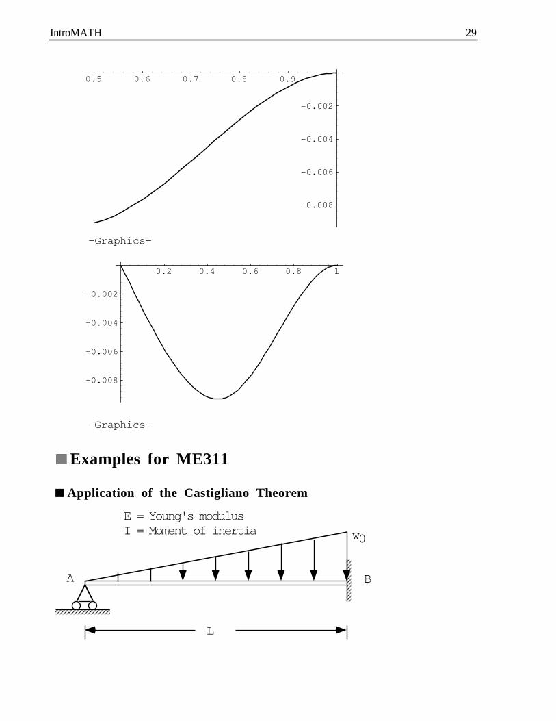
Examples for ME311

Application of the Castigliano Theorem

w0

L

A B

E = Young's modulusI = Moment of inertia

IntroMATH 29

We shall consider the same example for the statically inderminate beam bending with the linaerly distributed load with the hinge support at the left end ( x=0 ) and the fixed support at the right end ( x=L ), see the figure in above. Using this example, the reaction and the amount of the rotation of the beam are obtained at x=0. Noting the second Castigliano theorem yields the deflection of

the beam at the left end support ( x=0 ), the reaction Ra at this hinge support can be obtained by

solving the relation of the zero deflection at x=0 :

y yU

R R EIM x dx

EIM

M

Rdx

M x R x wx

Lx

x

aa a

L

a

L

a

= ( ) = = ( )

= =

( ) = −

∫ ∫01

21

0

12 3

2

0 0

0

∂∂

∂∂

∂∂

where

Translating these into Mathematica, we can solve the reaction Ra by using Solve command.

M=Ra*x-((1/2)*w0*(x/L)*x)*(x/3)ya=Integrate[M*D[M,Ra]/EI,{x,0,L}]Solve[ya==0,Ra]

3 w0 xRa x - ----- ---- 6 L

General::intinit: Loading integration packages.

3 4L Ra L w0----- - --------- ---- 3 EI 30 EI

L w0{{Ra -> ----}} --- 10

The slope of the deflection ( i.e. rotation of the beam ) at the left end hinge support x=0, can be obtained by applying the second Castigliano theorem after introducing a ficticious applied moment at the point where we wish to know the rotation. Indeed, if we translate this

θ ∂∂

∂∂x M M

L

a

U

M M EIM x dx

M x M R x wx

Lx

x

= → →= = ( )

( ) = − + −

∫0 0 0 0 0

2

0

0 0

0 0

12

12 3

lim lim

where

into Mathematica commnads, we can obtained the slope of the delection at x=0 as follows :

IntroMATH 30

M=-M0+Ra*x-((1/2)*w0*(x/L)*x)*(x/3)theta0=Integrate[M*D[M,M0]/EI,{x,0,L}]/.{M0->0}theta0=theta0/.{Ra->L*w0/10}

3 w0 x-M0 + Ra x - ----- ---- 6 L

2 3-(L Ra) L w0-------- + ------------ ---- 2 EI 24 EI

3-(L w0)--------------- 120 EI

Application of the Rayleigh-Ritz Method (1)

P

L/2 L/2

Young's Modulus EMoment of Inertia I

x

We shall obtain the deflection of the beam supported by a hinge at the left end and also fixed at the other end subject to a point load P at the center. The deflection of this beam was already obtained by integrating the second order differential equation written in terms of the bending moment M and the second derivative of the deflection as we have studied in ME210. We shall solve this problem by using the energy method that is one of the most important subjects covered in ME311. More precisely, we shall compute an approximated deflection, that should be very close to the exact solution, by the Rayleigh-Ritz method based on the principle of the minimum potential energy : the deflection in equilibrium minimizes the total potential energy, i.e., the total potential energy attains its minimum at the deflection that yields equilibrium of a structure. The total potential energy consists of the total strain energy and work potential :

F U W EId w

dxdx P w

LL= + =

− −( )

∫1

2 2

2

2

2

0

Note that the positive direction of the deflection is up-ward vertical direction, and the applied point force P is down-ward vertical. Thus, when we form the work potential, we must consider the applied force with the negative sign. The principle of the minimum potential energy says the deflection in equilibrium minimizes the total potential energy :

IntroMATH 31

min minw w

LF EI

d w

dxdx P w

L=

− −( )

∫1

2 2

2

2

2

0

Since the support condition must be satisfied with all of possible deflections for equilibrium, minimization of the total potential energy should be considered among deflections satisying the support condition. In this particular example, zero deflection at the left end, zero deflection and slope at the right end point must be satisfied :

w w Ldw

dxL0 0( ) = ( ) = ( ) =

If we parameterize possible deflections for equilibrium, e.g., by

w x x x L C C x C x( ) = −( ) + + +( )21 2 3

2 ..........

using "arbtirary" parameters C1, C2, C3, ......., we may determine these parameters so that the total potential energy is minimized. Then we can define the deflection that yields equilibrium of the structure. If possible deflections are parameterized, the total potential energy becomes a function of these parameters. If a finite number of parameters is used for approximation of a deflection, it becomes a function on a finite number of variables ( i.e. parameters ). Then the necessary condition of the minimum is vanishing the first derivatives of the function with respect to these variables :

∂∂

F

CC C C i

i1 2 3 0 1 2 3, , ,.......... , , ,.........( ) = =

This means that we can derive the same number of equations with the number of parameters introduced. Solving the set of equations with respect to the parameters yields the deflection that

minimizes the total potential energy, i.e., in equilibrium. Assuming only three parameters C1,

C2, and C3, we shall obtain the deflection using Mathematica.

IntroMATH 32

w2=x*(x-L)^2(C1+C2*x+C3*x^2)F=(EI/2)*Integrate[D[D[w2,x],x]^2,{x,0,L}]- (-P)*w2/.{x->L/2}F=Expand[F];Solve[{D[F,C1]==0,D[F,C2]==0,D[F,C3]==0}, {C1,C2,C3}]w2r=w2/.%//First

2 2x (-L + x) (C1 + C2 x + C3 x )

2 7 400 C3 L 3 2(EI (---------- + 4 L (-2 C1 + C2 L) + --------- 7 6 80 C3 L (C2 - 2 C3 L) + 3 2 12 L (-2 C1 + C2 L) (C1 - 2 C2 L + C3 L ) + 5 2 2 2 48 L (3 C2 + 5 C1 C3 - 22 C2 C3 L + 17 C3 L ) ------------------------------------------------ + ----------------------------------------------- 5 4 2 2 4 L (9 C1 C2 - 18 C2 L - 28 C1 C3 L + 50 C2 C3 L - 2 3 3 18 C3 L ) + 4 L 2 2 2 2 (3 C1 - 20 C1 C2 L + 16 C2 L + 22 C1 C3 L - 3 2 4 20 C2 C3 L + 3 C3 L ))) / 2 + 2 3 C2 L C3 L L (C1 + ---- + -----) P --- ---- 2 4 ------------------------ ----------------------- 8

-P -5 P{{C1 -> -----, C2 -> -------, C3 -> 0}} ---- ------ 32 EI 64 EI L

2 -P 5 P xx (-L + x) (----- - -------) ---- ------ 32 EI 64 EI L

IntroMATH 33

Plot[w2r/.{P->1,EI->1,L->1},{x,0,1}]

0.2 0.4 0.6 0.8 1

-0.008

-0.006

-0.004

-0.002

-Graphics-

Application of the Rayleigh-Ritz Method (2)

Deflection of the beam fixed at the both ends shown in the following figure, will be obtained by the Rayleigh-Ritz method based on the principle of minimum potential energy of a linearly elastic structure. A uniformly distributed load is applied on the right half portion of the beam with

intensity pd. For simplicity, let Young's modulus E be constant, and let the moment of inertia

of the cross section be also constant. The length of the beam is described by L. In the Rayleigh-Ritz method, approximated deflection of the beam must satisfy the support condition written in the deflection and its slope. Since the both ends are fixed, the deflection and slope must be zero at these points, i.e.,

w w Ldw

dx

dw

dxL0 0 0( ) = ( ) = ( ) = ( ) =

where w is the deflection, approximations wi of the deflection may be written by

w x x x L C C x C x C xi ii( ) = −( ) + + + +( )+

2 21 2 3

21...........

Substitution of this into the form of the total potential energy

F EId w

dxx dx p x w x dx

L

U

dL

L

W

= ( )

− ( ) ( )∫ ∫12

2

20

2

2

total strain energy work potential -1 2444 3444 1 244 344

yields a function F of a finite number of parameters C1, C2, ....., Ci+1 :

F C C C EId w

dxx dx p x w x dxi

iL

dL

L

i1 2 1

2

20

2

2

12

, ,......., +( ) = ( )

− ( ) ( )∫ ∫

IntroMATH 34

The necessary condition for the minimum of the total potential energy, that is approximated by

wi, is vanishing the gradient of F with respect to the parameters C1, C2,...., Ci+1 :

∂∂∂∂

∂∂

F

CC C C

F

CC C C

F

CC C C

i

i

ii

11 2 1

21 2 1

11 2 1

0

0

0

, ,....,

, ,....,

........................................

, ,....,

+

+

++

( ) =

( ) =

( ) =

Solving these i+1 number of equations in the i+1 parameters C1, C2, ....,Ci+1, we can

determine the deflection wi. We shall obtain the three approximated deflections for i = 0, 1, and

3 using Mathematica.

L/2 L/2

pdYoung's Modulus = EMoment of Inertia = I

Lowest Order Approximation

w0=x^2*(x-L)^2*(C1)F=(EI/2)*Integrate[D[D[w0,x],x]^2,{x,0,L}]- Integrate[pd*w0,{x,L/2,L}];F=Expand[F];Solve[D[F,C1]==0,C1]w0r=w0/.%//First

2 2C1 x (-L + x)

pd{{C1 -> -----}} ---- 48 EI

2 2pd x (-L + x)----------------------------- 48 EI

IntroMATH 35

Second Lowest Order Approximation

w1=x^2*(x-L)^2*(C1+C2*x)F=(EI/2)*Integrate[D[D[w1,x],x]^2,{x,0,L}]- Integrate[pd*w1,{x,L/2,L}];F=Expand[F];Solve[{D[F,C1]==0,D[F,C2]==0},{C1,C2}]w1r=w1/.%//First

2 2x (-L + x) (C1 + C2 x)

3 pd 7 pd{{C1 -> ------, C2 -> --------}} ----- ------- 256 EI 384 EI L

2 2 3 pd 7 pd xx (-L + x) (------ + --------) ----- ------- 256 EI 384 EI L

Third Order Ritz Approximation

w3=x^2*(x-L)^2*(C1+C2*x+C3*x^2+C4*x^3)F=(EI/2)*Integrate[D[D[w3,x],x]^2,{x,0,L}]- Integrate[pd*w3,{x,L/2,L}];F=Expand[F];Solve[{D[F,C1]==0,D[F,C2]==0,D[F,C3]==0,D[F,C4]==0}, {C1,C2,C3,C4}]w3r=w3/.%//First

2 2 2 3x (-L + x) (C1 + C2 x + C3 x + C4 x )

83 pd pd 33 pd{{C1 -> -------, C2 -> --------, C3 -> ----------, ------ ------- --------- 6144 EI 256 EI L 2 1024 EI L -11 pd C4 -> ---------}} -------- 3 512 EI L

2 3 2 2 83 pd pd x 33 pd x 11 pd xx (-L + x) (------- + -------- + ---------- - ---------) ------ ------- --------- -------- 6144 EI 256 EI L 2 3 1024 EI L 512 EI L

Graphs of the three approximations

Since the 1st order and the 3rd order Ritz approximations are almost identical, we can say that the deflection of a beam can be obtained using rather few terms of a polynomial with sufficient accuracy.

IntroMATH 36

Plot[{w0r/.{pd->1,EI->1,L->1}, w1r/.{pd->1,EI->1,L->1}, w3r/.{pd->1,EI->1,L->1}},{x,0,1}]

0.2 0.4 0.6 0.8 1

0.0002

0.0004

0.0006

0.0008

0.001

0.0012

-Graphics-

Example of a Plane Frame Structure

In above, we present examples of a beam that can be analyzied by the method studied in ME210. Here we shall provide an example of the plane frame structure, shown in the following figure, that might not be solved by the method studied in ME210.

p0

L L

L

A

B C

D

Rx

Ry

The frame structure consists of three beams, the length of which is the same, say L. At point A, it is fixed, i.e., the deflection and rotation ( the slope of the deflection ) are constrained to be zero,

while it is supported by a hinge at D. A uniformly distributed load, p0, is applied along the

IntroMATH 37

member AB. Since this is a plane frame, we must consider at least bending and axial deformation. Shear effect can be neglected, and torsion is not involved. We shall obtain the

reaction forces Rx and Ry at the hinge support D using the energy method, more precisely, by

applying the second Castigliano theorem. Noting that point D is supported by a hinge, both x and y components of the displacement are zero, the Castigliano therem implies that

δ ∂∂

δ ∂∂x

xy

y

U

R

U

R= = = =

* *

0 0 and

where U* is the total complementary strain energy that must be the same with the total strain energy for any linearly elastic structure :

UM

EIds

N

EAdsi

i

i

i

LL

i

nii* = +

∫∫∑

=

12

2 2

001

Here n is the total number of members consisting of a given frame structure, Li is the length, Mi

is the bending moment, Ni is the axial force, EIi is the bending rigidity, EAi is the rigidity of

member i in the axial deformation, and s is the coordinate defined in each member along the beam axis. Noting that the axial force and bending moment are given by

N

R

R

R

y

x

y

=

−

in member CD

in member BC

in member AB

and

M

R s

R L R s

R L RLyL RLxs pL ss

x

x y

x

=−− −

− − + + ( )

in member CD

in member BC

in member AB02

we can set up the following Mathematica program to find the reactions at D :

IntroMATH 38

N1=-Ry;M1=-Rx*s;N2=Rx;M2=-Rx*L-Ry*s;N3=Ry;M3=-Rx*L-Ry*L+Rx*s+(p0*s)*s/2;UN=(Integrate[N1^2,{s,0,L}]+ Integrate[N2^2,{s,0,L}]+ Integrate[N3^2,{s,0,L}])/(2*EA);UM=(Integrate[M1^2,{s,0,L}]+ Integrate[M2^2,{s,0,L}]+ Integrate[M3^2,{s,0,L}])/(2*EI);deltax=Simplify[D[UN+UM,Rx]]deltay=Simplify[D[UN+UM,Ry]]Solve[{deltax==0,deltay==0},{Rx,Ry}]{Rx,Ry}=Simplify[{Rx,Ry}/.%//First]

3L Rx L (-(L p0) + 40 Rx + 24 Ry)---- + ------------------------------- --------------------------- EA 24 EI

General::spell1: Possible spelling error: new symbol name "deltay" is similar to existing symbol "deltax".

32 L Ry L (-(L p0) + 6 Rx + 8 Ry)------ + ------------------------------- ------------------------- EA 6 EI

L p0 2{{Rx -> ---- + (2 (3 EI + 2 EA L ) --- 6 2 5 3 2 (-6 EA L p0 + 8 EA L (3 EI + 5 EA L ) p0)) / 2 2 2 2 4 (3 EA L (-288 EI - 672 EA EI L - 176 EA L )), 2 5 3 2 Ry -> -((-6 EA L p0 + 8 EA L (3 EI + 5 EA L ) p0) / 2 2 2 4 (-288 EI - 672 EA EI L - 176 EA L ))}}

3 2 EA L (3 EI - 4 EA L ) p0{------------------------------------, ----------------------------------- 2 2 2 4 4 (18 EI + 42 EA EI L + 11 EA L ) 3 2 EA L (12 EI + 17 EA L ) p0 ------------------------------------} ----------------------------------- 2 2 2 4 8 (18 EI + 42 EA EI L + 11 EA L )

IntroMATH 39

Examples in ME305

1 2

34

ξ

η

2

2

We shall make an analysis of finite element interpolation error of the 4 node quadrilateral element for plane problems using Taylor's exansion of an arbitrary function g in Mathematica :

g s t s s t ti j

g

s ts t O s s t t

i ji j

i jji

g s t

0 0 0 0

0

2

0

2

03

031

2 0 0

,! !

, ,

,

( ) = −( ) −( ) ( ) + −( ) −( )( )+

==

= ( )

∑∑ ∂∂ ∂

1 24444444 34444444

The shape functions of the 4 node quadrilateral element are

N s t s t N s t s t

N s t s t N s t s t

1 2

3 4

14

1 114

1 1

14

1 114

1 1

, ,

, ,

( ) = −( ) −( ) ( ) = +( ) −( )

( ) = +( ) +( ) ( ) = −( ) +( )

,

,

Then the first derivatives of the interpolation error may be represented by

∂∂

∂∂

∂∂

∂∂

∂∂

∂∂

e

sg s t

N

ss t

g

s

e

tg s t

N

ts t

g

sI

i

i ii I

i

i ii= ( ) ( ) − = ( ) ( ) −

= =∑ ∑2

1

4

2

1

4

, , , , ,

IntroMATH 40

gT2=Normal[Series[g[s0,t0],{s0,s,2},{t0,t,2}]]g1=gT2/.{s0->-1,t0->-1};g2=gT2/.{s0-> 1,t0->-1};g3=gT2/.{s0-> 1,t0-> 1};g4=gT2/.{s0->-1,t0-> 1};gv={g1,g2,g3,g4};SF={(1-s)*(1-t)/4, (1+s)*(1-t)/4, (1+s)*(1+t)/4, (1-s)*(1+t)/4}deds=Simplify[gv.D[SF,s]-Derivative[1,0][g][s,t]]dedt=Simplify[gv.D[SF,t]-Derivative[0,1][g][s,t]]

(1,0)g[s, t] + (-s + s0) g [s, t] + 2 (2,0) (-s + s0) g [s, t] ----------------------- + ---------------------- 2 (0,1) (1,1) (-t + t0) (g [s, t] + (-s + s0) g [s, t] + 2 (2,1) (-s + s0) g [s, t] -----------------------) + ---------------------- 2 (0,2) (1,2) 2 g [s, t] (-s + s0) g [s, t] (-t + t0) (------------ + ---------------------- + ----------- --------------------- 2 2 2 (2,2) (-s + s0) g [s, t] -----------------------) ---------------------- 4

(1,2) 2 (1,2) (2,0)(g [s, t] - t g [s, t] - 2 s g [s, t] - (2,2) 2 (2,2) s g [s, t] + s t g [s, t]) / 2

General::spell1: Possible spelling error: new symbol name "dedt" is similar to existing symbol "deds".

(0,2) (2,1) 2 (2,1)(-2 t g [s, t] + g [s, t] - s g [s, t] - (2,2) 2 (2,2) t g [s, t] + s t g [s, t]) / 2

For the geometry described in the following figure, we shall consider the case of pure bending chracterized by the deformed configuration shown in the figure using the bold face. We shall

compute the normal strains, ex and ey, and shear strain, gxy, of this deformation, and the

normalized strain energies, Ix,Iy, and Ixy, due to these three strains with respect to E/(1-v^2),

where E is Young's modulus and v is Poisson's ratio. After obtaining these strain energies, we

shall plot the ratio Ixy/Ix with respect to the element geometry aspect ratio hy/hx.

IntroMATH 41

1 2

34

hx

x

hy

xv={0,hx,hx,0}yv={0,0,hy,hy}jac={{xv.D[SF,s],yv.D[SF,s]}, {xv.D[SF,t],yv.D[SF,t]}};MatrixForm[jac]jacobian=jac[[1,1]]*jac[[2,2]]-jac[[2,1]]*jac[[1,2]];jacinv=Simplify[Inverse[jac]];MatrixForm[jacinv]uv={-a,a,-a,a}duds=Simplify[uv.D[SF,s]];dudt=Simplify[uv.D[SF,t]];vv={0,0,0,0}dvds=Simplify[vv.D[SF,s]];dvdt=Simplify[vv.D[SF,t]];ex=jacinv[[1,1]]*duds+jacinv[[1,2]]*dudt;ey=jacinv[[2,1]]*dvds+jacinv[[2,2]]*dvdt;gxy=jacinv[[1,1]]*dvds+jacinv[[1,2]]*dvdt+ jacinv[[2,1]]*duds+jacinv[[2,2]]*dudt;ex=Simplify[ex]ey=Simplify[ey]gxy=Simplify[gxy]Ix=Integrate[(ex^2)*jacobian,{s,-1,1},{t,-1,1}];Iy=Integrate[(ey^2)*jacobian,{s,-1,1},{t,-1,1}];Ixy=Integrate[(gxy^2)*jacobian,{s,-1,1},{t,-1,1}];Ix=Simplify[Ix]Iy=Simplify[Iy]Ixy=Simplify[Ixy]pr=0.3;d33=(1-pr)/2;Plot[(d33*Ixy/.{hy->x*hx,a->1})/(Ix/.{hy->x*hx,a->1}), {x,0.5,4}]

{0, hx, hx, 0}

{0, 0, hy, hy}

IntroMATH 42

hx (1 - t) hx (1 + t)---------- + ------------------- --------- 4 4 0 hy (1 - s) hy (1 + s) ---------- + ---------- --------- --------- 0 4 4

2--- hx 0 2 -- - 0 hy

{-a, a, -a, a}

{0, 0, 0, 0}

-2 a t----------- hx

0

-2 a s----------- hy

24 a hy------------- 3 hx

0

24 a hx------------- 3 hy

1 2 3 4

0.2

0.4

0.6

0.8

1

1.2

1.4

-Graphics-

IntroMATH 43