introduction to probability - wordpress.com
TRANSCRIPT

Introduction to Probability
Charles M. Grinstead
Swarthmore College
J. Laurie Snell
Dartmouth College

To our wives
and in memory of
Reese T. Prosser

Contents
1 Discrete Probability Distributions 11.1 Simulation of Discrete Probabilities . . . . . . . . . . . . . . . . . . . 11.2 Discrete Probability Distributions . . . . . . . . . . . . . . . . . . . . 18
2 Continuous Probability Densities 412.1 Simulation of Continuous Probabilities . . . . . . . . . . . . . . . . . 412.2 Continuous Density Functions . . . . . . . . . . . . . . . . . . . . . . 55
3 Combinatorics 753.1 Permutations . . . . . . . . . . . . . . . . . . . . . . . . . . . . . . . 753.2 Combinations . . . . . . . . . . . . . . . . . . . . . . . . . . . . . . . 923.3 Card Shuffling . . . . . . . . . . . . . . . . . . . . . . . . . . . . . . . 120
4 Conditional Probability 1334.1 Discrete Conditional Probability . . . . . . . . . . . . . . . . . . . . 1334.2 Continuous Conditional Probability . . . . . . . . . . . . . . . . . . . 1624.3 Paradoxes . . . . . . . . . . . . . . . . . . . . . . . . . . . . . . . . . 175
5 Distributions and Densities 1835.1 Important Distributions . . . . . . . . . . . . . . . . . . . . . . . . . 1835.2 Important Densities . . . . . . . . . . . . . . . . . . . . . . . . . . . 205
6 Expected Value and Variance 2256.1 Expected Value . . . . . . . . . . . . . . . . . . . . . . . . . . . . . . 2256.2 Variance of Discrete Random Variables . . . . . . . . . . . . . . . . . 2576.3 Continuous Random Variables . . . . . . . . . . . . . . . . . . . . . . 268
7 Sums of Random Variables 2857.1 Sums of Discrete Random Variables . . . . . . . . . . . . . . . . . . 2857.2 Sums of Continuous Random Variables . . . . . . . . . . . . . . . . . 291
8 Law of Large Numbers 3058.1 Discrete Random Variables . . . . . . . . . . . . . . . . . . . . . . . 3058.2 Continuous Random Variables . . . . . . . . . . . . . . . . . . . . . . 316
v

vi CONTENTS
9 Central Limit Theorem 3259.1 Bernoulli Trials . . . . . . . . . . . . . . . . . . . . . . . . . . . . . . 3259.2 Discrete Independent Trials . . . . . . . . . . . . . . . . . . . . . . . 3409.3 Continuous Independent Trials . . . . . . . . . . . . . . . . . . . . . 355
10 Generating Functions 36510.1 Discrete Distributions . . . . . . . . . . . . . . . . . . . . . . . . . . 36510.2 Branching Processes . . . . . . . . . . . . . . . . . . . . . . . . . . . 37710.3 Continuous Densities . . . . . . . . . . . . . . . . . . . . . . . . . . . 394
11 Markov Chains 40511.1 Introduction . . . . . . . . . . . . . . . . . . . . . . . . . . . . . . . . 40511.2 Absorbing Markov Chains . . . . . . . . . . . . . . . . . . . . . . . . 41511.3 Ergodic Markov Chains . . . . . . . . . . . . . . . . . . . . . . . . . 43311.4 Fundamental Limit Theorem . . . . . . . . . . . . . . . . . . . . . . 44711.5 Mean First Passage Time . . . . . . . . . . . . . . . . . . . . . . . . 452
12 Random Walks 47112.1 Random Walks in Euclidean Space . . . . . . . . . . . . . . . . . . . 47112.2 Gambler’s Ruin . . . . . . . . . . . . . . . . . . . . . . . . . . . . . . 48612.3 Arc Sine Laws . . . . . . . . . . . . . . . . . . . . . . . . . . . . . . . 493
Appendices 499A Normal Distribution Table . . . . . . . . . . . . . . . . . . . . . . . . 499B Galton’s Data . . . . . . . . . . . . . . . . . . . . . . . . . . . . . . . 500C Life Table . . . . . . . . . . . . . . . . . . . . . . . . . . . . . . . . . 501
Index 503

Preface
Probability theory began in seventeenth century France when the two great Frenchmathematicians, Blaise Pascal and Pierre de Fermat, corresponded over two prob-lems from games of chance. Problems like those Pascal and Fermat solved continuedto influence such early researchers as Huygens, Bernoulli, and DeMoivre in estab-lishing a mathematical theory of probability. Today, probability theory is a well-established branch of mathematics that finds applications in every area of scholarlyactivity from music to physics, and in daily experience from weather prediction topredicting the risks of new medical treatments.
This text is designed for an introductory probability course taken by sophomores,juniors, and seniors in mathematics, the physical and social sciences, engineering,and computer science. It presents a thorough treatment of probability ideas andtechniques necessary for a firm understanding of the subject. The text can be usedin a variety of course lengths, levels, and areas of emphasis.
For use in a standard one-term course, in which both discrete and continuousprobability is covered, students should have taken as a prerequisite two terms ofcalculus, including an introduction to multiple integrals. In order to cover Chap-ter 11, which contains material on Markov chains, some knowledge of matrix theoryis necessary.
The text can also be used in a discrete probability course. The material has beenorganized in such a way that the discrete and continuous probability discussions arepresented in a separate, but parallel, manner. This organization dispels an overlyrigorous or formal view of probability and offers some strong pedagogical valuein that the discrete discussions can sometimes serve to motivate the more abstractcontinuous probability discussions. For use in a discrete probability course, studentsshould have taken one term of calculus as a prerequisite.
Very little computing background is assumed or necessary in order to obtain fullbenefits from the use of the computing material and examples in the text. All ofthe programs that are used in the text have been written in each of the languagesTrueBASIC, Maple, and Mathematica.
This book is on the Web at http://www.dartmouth.edu/ chance, and is part ofthe Chance project, which is devoted to providing materials for beginning courses inprobability and statistics. The computer programs, solutions to the odd-numberedexercises, and current errata are also available at this site. Instructors may obtainall of the solutions by writing to either of the authors, at [email protected] [email protected]. It is our intention to place items related to this book at
vii

viii PREFACE
this site, and we invite our readers to submit their contributions.
FEATURES
Level of rigor and emphasis: Probability is a wonderfully intuitive and applicablefield of mathematics. We have tried not to spoil its beauty by presenting too muchformal mathematics. Rather, we have tried to develop the key ideas in a somewhatleisurely style, to provide a variety of interesting applications to probability, and toshow some of the nonintuitive examples that make probability such a lively subject.
Exercises: There are over 600 exercises in the text providing plenty of oppor-tunity for practicing skills and developing a sound understanding of the ideas. Inthe exercise sets are routine exercises to be done with and without the use of acomputer and more theoretical exercises to improve the understanding of basic con-cepts. More difficult exercises are indicated by an asterisk. A solution manual forall of the exercises is available to instructors.
Historical remarks: Introductory probability is a subject in which the funda-mental ideas are still closely tied to those of the founders of the subject. For thisreason, there are numerous historical comments in the text, especially as they dealwith the development of discrete probability.
Pedagogical use of computer programs: Probability theory makes predictionsabout experiments whose outcomes depend upon chance. Consequently, it lendsitself beautifully to the use of computers as a mathematical tool to simulate andanalyze chance experiments.
In the text the computer is utilized in several ways. First, it provides a labora-tory where chance experiments can be simulated and the students can get a feelingfor the variety of such experiments. This use of the computer in probability hasbeen already beautifully illustrated by William Feller in the second edition of hisfamous text An Introduction to Probability Theory and Its Applications (New York:Wiley, 1950). In the preface, Feller wrote about his treatment of fluctuation in cointossing: “The results are so amazing and so at variance with common intuitionthat even sophisticated colleagues doubted that coins actually misbehave as theorypredicts. The record of a simulated experiment is therefore included.”
In addition to providing a laboratory for the student, the computer is a powerfulaid in understanding basic results of probability theory. For example, the graphicalillustration of the approximation of the standardized binomial distributions to thenormal curve is a more convincing demonstration of the Central Limit Theoremthan many of the formal proofs of this fundamental result.
Finally, the computer allows the student to solve problems that do not lendthemselves to closed-form formulas such as waiting times in queues. Indeed, theintroduction of the computer changes the way in which we look at many problemsin probability. For example, being able to calculate exact binomial probabilitiesfor experiments up to 1000 trials changes the way we view the normal and Poissonapproximations.

PREFACE ix
ACKNOWLEDGMENTS FOR FIRST EDITION
Anyone writing a probability text today owes a great debt to William Feller,who taught us all how to make probability come alive as a subject matter. If youfind an example, an application, or an exercise that you really like, it probably hadits origin in Feller’s classic text, An Introduction to Probability Theory and Its
Applications.
This book had its start with a course given jointly at Dartmouth College withProfessor John Kemeny. I am indebted to Professor Kemeny for convincing me thatit is both useful and fun to use the computer in the study of probability. He hascontinuously and generously shared his ideas on probability and computing withme. No less impressive has been the help of John Finn in making the computingan integral part of the text and in writing the programs so that they not onlycan be easily used, but they also can be understood and modified by the student toexplore further problems. Some of the programs in the text were developed throughcollaborative efforts with John Kemeny and Thomas Kurtz on a Sloan Foundationproject and with John Finn on a Keck Foundation project. I am grateful to bothfoundations for their support.
I am indebted to many other colleagues, students, and friends for valuable com-ments and suggestions. A few whose names stand out are: Eric and Jim Baum-gartner, Tom Bickel, Bob Beck, Ed Brown, Christine Burnley, Richard Crowell,David Griffeath, John Lamperti, Beverly Nickerson, Reese Prosser, Cathy Smith,and Chris Thron.
The following individuals were kind enough to review various drafts of themanuscript. Their encouragement, criticisms, and suggestions were very helpful.
Ron Barnes University of Houston, Downtown CollegeThomas Fischer Texas A & M UniversityRichard Groeneveld Iowa State UniversityJames Kuelbs University of Wisconsin, MadisonGreg Lawler Duke UniversitySidney Resnick Colorado State UniversityMalcom Sherman SUNY AlbanyOlaf Stackelberg Kent State UniversityMurad Taqqu Boston UniversityAbraham Wender University of North Carolina
In addition, I would especially like to thank James Kuelbs, Sidney Resnick, andtheir students for using the manuscript in their courses and sharing their experienceand invaluable suggestions with me.
The versatility of Dartmouth’s mathematical word processor PREPPY, writtenby Professor James Baumgartner, has made it much easier to make revisions, but hasmade the job of typist extraordinaire Marie Slack correspondingly more challenging.Her high standards and willingness always to try the next more difficult task havemade it all possible.
Finally, I must thank all the people at Random House who helped during the de-

x PREFACE
velopment and production of this project. First, among these was my editor WayneYuhasz, whose continued encouragement and commitment were very helpful duringthe development of the manuscript. The entire production team provided efficientand professional support: Margaret Pinette, project manager; Michael Weinstein,production manager; and Kate Bradfor of Editing, Design, and Production, Inc.
ACKNOWLEDGMENTS FOR SECOND EDITION
The debt to William Feller has not diminished in the years between the twoeditions of this book. His book on probability is likely to remain the classic bookin this field for many years.
The process of revising the first edition of this book began with some high-leveldiscussions involving the two present co-authors together with Reese Prosser andJohn Finn. It was during these discussions that, among other things, the first co-author was made aware of the concept of “negative royalties” by Professor Prosser.
We are indebted to many people for their help in this undertaking. First andforemost, we thank Mark Kernighan for his almost 40 pages of single-spaced com-ments on the first edition. Many of these comments were very thought-provoking;in addition, they provided a student’s perspective on the book. Most of the majorchanges in the second edition have their genesis in these notes.
We would also like to thank Fuxing Hou, who provided extensive help with thetypesetting and the figures. Her incessant good humor in the face of many trials,both big (“we need to change the entire book from Lamstex to Latex”) and small(“could you please move this subscript down just a bit?”), was truly remarkable.
We would also like to thank Lee Nave, who typed the entire first edition of thebook into the computer. Lee corrected most of the typographical errors in the firstedition during this process, making our job easier.
Karl Knaub and Jessica Sklar are responsible for the implementations of thecomputer programs in Mathematica and Maple, and we thank them for their efforts.We also thank Jessica for her work on the solution manual for the exercises, buildingon the work done by Gang Wang for the first edition.
Tom Shemanske and Dana Williams provided much TeX-nical assistance. Theirpatience and willingness to help, even to the extent of writing intricate TeX macros,are very much appreciated.
The following people used various versions of the second edition in their proba-bility courses, and provided valuable comments and criticisms.
Marty Arkowitz Dartmouth CollegeAimee Johnson Swarthmore CollegeBill Peterson Middlebury CollegeDan Rockmore Dartmouth CollegeShunhui Zhu Dartmouth College
Reese Prosser and John Finn provided much in the way of moral support andcamaraderie throughout this project. Certainly, one of the high points of this entire

PREFACE xi
endeavour was Professor Prosser’s telephone call to a casino in Monte Carlo, in anattempt to find out the rules involving the “prison” in roulette.
Peter Doyle motivated us to make this book part of a larger project on the Web,to which others can contribute. He also spent many hours actually carrying out theoperation of putting the book on the Web.
Finally, we thank Sergei Gelfand and the American Mathematical Society fortheir interest in our book, their help in its production, and their willingness to letus put the book on the Web.


Chapter 1
Discrete ProbabilityDistributions
1.1 Simulation of Discrete Probabilities
Probability
In this chapter, we shall first consider chance experiments with a finite number ofpossible outcomes ω1, ω2, . . . , ωn. For example, we roll a die and the possibleoutcomes are 1, 2, 3, 4, 5, 6 corresponding to the side that turns up. We toss a coinwith possible outcomes H (heads) and T (tails).
It is frequently useful to be able to refer to an outcome of an experiment. Forexample, we might want to write the mathematical expression which gives the sumof four rolls of a die. To do this, we could let Xi, i = 1, 2, 3, 4, represent the valuesof the outcomes of the four rolls, and then we could write the expression
X1 +X2 +X3 +X4
for the sum of the four rolls. The Xi’s are called random variables. A random vari-able is simply an expression whose value is the outcome of a particular experiment.Just as in the case of other types of variables in mathematics, random variables cantake on different values.
Let X be the random variable which represents the roll of one die. We shallassign probabilities to the possible outcomes of this experiment. We do this byassigning to each outcome ωj a nonnegative number m(ωj) in such a way that
m(ω1) +m(ω2) + · · ·+m(ω6) = 1 .
The function m(ωj) is called the distribution function of the random variable X.For the case of the roll of the die we would assign equal probabilities or probabilities1/6 to each of the outcomes. With this assignment of probabilities, one could write
P (X ≤ 4) =23
1

2 CHAPTER 1. DISCRETE PROBABILITY DISTRIBUTIONS
to mean that the probability is 2/3 that a roll of a die will have a value which doesnot exceed 4.
Let Y be the random variable which represents the toss of a coin. In this case,there are two possible outcomes, which we can label as H and T. Unless we havereason to suspect that the coin comes up one way more often than the other way,it is natural to assign the probability of 1/2 to each of the two outcomes.
In both of the above experiments, each outcome is assigned an equal probability.This would certainly not be the case in general. For example, if a drug is found tobe effective 30 percent of the time it is used, we might assign a probability .3 thatthe drug is effective the next time it is used and .7 that it is not effective. This lastexample illustrates the intuitive frequency concept of probability. That is, if we havea probability p that an experiment will result in outcome A, then if we repeat thisexperiment a large number of times we should expect that the fraction of times thatA will occur is about p. To check intuitive ideas like this, we shall find it helpful tolook at some of these problems experimentally. We could, for example, toss a coina large number of times and see if the fraction of times heads turns up is about 1/2.We could also simulate this experiment on a computer.
Simulation
We want to be able to perform an experiment that corresponds to a given set ofprobabilities; for example, m(ω1) = 1/2, m(ω2) = 1/3, and m(ω3) = 1/6. In thiscase, one could mark three faces of a six-sided die with an ω1, two faces with an ω2,and one face with an ω3.
In the general case we assume that m(ω1), m(ω2), . . . , m(ωn) are all rationalnumbers, with least common denominator n. If n > 2, we can imagine a longcylindrical die with a cross-section that is a regular n-gon. If m(ωj) = nj/n, thenwe can label nj of the long faces of the cylinder with an ωj , and if one of the endfaces comes up, we can just roll the die again. If n = 2, a coin could be used toperform the experiment.
We will be particularly interested in repeating a chance experiment a large num-ber of times. Although the cylindrical die would be a convenient way to carry outa few repetitions, it would be difficult to carry out a large number of experiments.Since the modern computer can do a large number of operations in a very shorttime, it is natural to turn to the computer for this task.
Random Numbers
We must first find a computer analog of rolling a die. This is done on the computerby means of a random number generator. Depending upon the particular softwarepackage, the computer can be asked for a real number between 0 and 1, or an integerin a given set of consecutive integers. In the first case, the real numbers are chosenin such a way that the probability that the number lies in any particular subintervalof this unit interval is equal to the length of the subinterval. In the second case,each integer has the same probability of being chosen.

1.1. SIMULATION OF DISCRETE PROBABILITIES 3
.203309 .762057 .151121 .623868
.932052 .415178 .716719 .967412
.069664 .670982 .352320 .049723
.750216 .784810 .089734 .966730
.946708 .380365 .027381 .900794
Table 1.1: Sample output of the program RandomNumbers.
Let X be a random variable with distribution function m(ω), where ω is in theset ω1, ω2, ω3, and m(ω1) = 1/2, m(ω2) = 1/3, and m(ω3) = 1/6. If our computerpackage can return a random integer in the set 1, 2, ..., 6, then we simply ask itto do so, and make 1, 2, and 3 correspond to ω1, 4 and 5 correspond to ω2, and 6correspond to ω3. If our computer package returns a random real number r in theinterval (0, 1), then the expression
b6rc+ 1
will be a random integer between 1 and 6. (The notation bxc means the greatestinteger not exceeding x, and is read “floor of x.”)
The method by which random real numbers are generated on a computer isdescribed in the historical discussion at the end of this section. The followingexample gives sample output of the program RandomNumbers.
Example 1.1 (Random Number Generation) The program RandomNumbersgenerates n random real numbers in the interval [0, 1], where n is chosen by theuser. When we ran the program with n = 20, we obtained the data shown inTable 1.1. 2
Example 1.2 (Coin Tossing) As we have noted, our intuition suggests that theprobability of obtaining a head on a single toss of a coin is 1/2. To have thecomputer toss a coin, we can ask it to pick a random real number in the interval[0, 1] and test to see if this number is less than 1/2. If so, we shall call the outcomeheads; if not we call it tails. Another way to proceed would be to ask the computerto pick a random integer from the set 0, 1. The program CoinTosses carriesout the experiment of tossing a coin n times. Running this program, with n = 20,resulted in:
THTTTHTTTTHTTTTTHHTT.
Note that in 20 tosses, we obtained 5 heads and 15 tails. Let us toss a coin n
times, where n is much larger than 20, and see if we obtain a proportion of headscloser to our intuitive guess of 1/2. The program CoinTosses keeps track of thenumber of heads. When we ran this program with n = 1000, we obtained 494 heads.When we ran it with n = 10000, we obtained 5039 heads.

4 CHAPTER 1. DISCRETE PROBABILITY DISTRIBUTIONS
We notice that when we tossed the coin 10,000 times, the proportion of headswas close to the “true value” .5 for obtaining a head when a coin is tossed. A math-ematical model for this experiment is called Bernoulli Trials (see Chapter 3). TheLaw of Large Numbers, which we shall study later (see Chapter 8), will show thatin the Bernoulli Trials model, the proportion of heads should be near .5, consistentwith our intuitive idea of the frequency interpretation of probability.
Of course, our program could be easily modified to simulate coins for which theprobability of a head is p, where p is a real number between 0 and 1. 2
In the case of coin tossing, we already knew the probability of the event occurringon each experiment. The real power of simulation comes from the ability to estimateprobabilities when they are not known ahead of time. This method has been used inthe recent discoveries of strategies that make the casino game of blackjack favorableto the player. We illustrate this idea in a simple situation in which we can computethe true probability and see how effective the simulation is.
Example 1.3 (Dice Rolling) We consider a dice game that played an importantrole in the historical development of probability. The famous letters between Pas-cal and Fermat, which many believe started a serious study of probability, wereinstigated by a request for help from a French nobleman and gambler, Chevalierde Mere. It is said that de Mere had been betting that, in four rolls of a die, atleast one six would turn up. He was winning consistently and, to get more peopleto play, he changed the game to bet that, in 24 rolls of two dice, a pair of sixeswould turn up. It is claimed that de Mere lost with 24 and felt that 25 rolls werenecessary to make the game favorable. It was un grand scandale that mathematicswas wrong.
We shall try to see if de Mere is correct by simulating his various bets. Theprogram DeMere1 simulates a large number of experiments, seeing, in each one,if a six turns up in four rolls of a die. When we ran this program for 1000 plays,a six came up in the first four rolls 48.6 percent of the time. When we ran it for10,000 plays this happened 51.98 percent of the time.
We note that the result of the second run suggests that de Mere was correctin believing that his bet with one die was favorable; however, if we had based ourconclusion on the first run, we would have decided that he was wrong. Accurateresults by simulation require a large number of experiments. 2
The program DeMere2 simulates de Mere’s second bet that a pair of sixeswill occur in n rolls of a pair of dice. The previous simulation shows that it isimportant to know how many trials we should simulate in order to expect a certaindegree of accuracy in our approximation. We shall see later that in these types ofexperiments, a rough rule of thumb is that, at least 95% of the time, the error doesnot exceed the reciprocal of the square root of the number of trials. Fortunately,for this dice game, it will be easy to compute the exact probabilities. We shallshow in the next section that for the first bet the probability that de Mere wins is1− (5/6)4 = .518.

1.1. SIMULATION OF DISCRETE PROBABILITIES 5
5 10 15 20 25 30 35 40
-10
-8
-6
-4
-2
2
4
6
8
10
Figure 1.1: Peter’s winnings in 40 plays of heads or tails.
One can understand this calculation as follows: The probability that no 6 turnsup on the first toss is (5/6). The probability that no 6 turns up on either of thefirst two tosses is (5/6)2. Reasoning in the same way, the probability that no 6turns up on any of the first four tosses is (5/6)4. Thus, the probability of at leastone 6 in the first four tosses is 1 − (5/6)4. Similarly, for the second bet, with 24rolls, the probability that de Mere wins is 1 − (35/36)24 = .491, and for 25 rolls itis 1− (35/36)25 = .506.
Using the rule of thumb mentioned above, it would require 27,000 rolls to have areasonable chance to determine these probabilities with sufficient accuracy to assertthat they lie on opposite sides of .5. It is interesting to ponder whether a gamblercan detect such probabilities with the required accuracy from gambling experience.Some writers on the history of probability suggest that de Mere was, in fact, justinterested in these problems as intriguing probability problems.
Example 1.4 (Heads or Tails) For our next example, we consider a problem wherethe exact answer is difficult to obtain but for which simulation easily gives thequalitative results. Peter and Paul play a game called heads or tails. In this game,a fair coin is tossed a sequence of times—we choose 40. Each time a head comes upPeter wins 1 penny from Paul, and each time a tail comes up Peter loses 1 pennyto Paul. For example, if the results of the 40 tosses are
THTHHHHTTHTHHTTHHTTTTHHHTHHTHHHTHHHTTTHH.
Peter’s winnings may be graphed as in Figure 1.1.Peter has won 6 pennies in this particular game. It is natural to ask for the
probability that he will win j pennies; here j could be any even number from −40to 40. It is reasonable to guess that the value of j with the highest probabilityis j = 0, since this occurs when the number of heads equals the number of tails.Similarly, we would guess that the values of j with the lowest probabilities arej = ±40.

6 CHAPTER 1. DISCRETE PROBABILITY DISTRIBUTIONS
A second interesting question about this game is the following: How many timesin the 40 tosses will Peter be in the lead? Looking at the graph of his winnings(Figure 1.1), we see that Peter is in the lead when his winnings are positive, butwe have to make some convention when his winnings are 0 if we want all tosses tocontribute to the number of times in the lead. We adopt the convention that, whenPeter’s winnings are 0, he is in the lead if he was ahead at the previous toss andnot if he was behind at the previous toss. With this convention, Peter is in the lead34 times in our example. Again, our intuition might suggest that the most likelynumber of times to be in the lead is 1/2 of 40, or 20, and the least likely numbersare the extreme cases of 40 or 0.
It is easy to settle this by simulating the game a large number of times andkeeping track of the number of times that Peter’s final winnings are j, and thenumber of times that Peter ends up being in the lead by k. The proportions overall games then give estimates for the corresponding probabilities. The programHTSimulation carries out this simulation. Note that when there are an evennumber of tosses in the game, it is possible to be in the lead only an even numberof times. We have simulated this game 10,000 times. The results are shown inFigures 1.2 and 1.3. These graphs, which we call spike graphs, were generatedusing the program Spikegraph. The vertical line, or spike, at position x on thehorizontal axis, has a height equal to the proportion of outcomes which equal x.Our intuition about Peter’s final winnings was quite correct, but our intuition aboutthe number of times Peter was in the lead was completely wrong. The simulationsuggests that the least likely number of times in the lead is 20 and the most likelyis 0 or 40. This is indeed correct, and the explanation for it is suggested by playingthe game of heads or tails with a large number of tosses and looking at a graph ofPeter’s winnings. In Figure 1.4 we show the results of a simulation of the game, for1000 tosses and in Figure 1.5 for 10,000 tosses.
In the second example Peter was ahead most of the time. It is a remarkablefact, however, that, if play is continued long enough, Peter’s winnings will continueto come back to 0, but there will be very long times between the times that thishappens. These and related results will be discussed in Chapter 12. 2
In all of our examples so far, we have simulated equiprobable outcomes. Weillustrate next an example where the outcomes are not equiprobable.
Example 1.5 (Horse Races) Four horses (Acorn, Balky, Chestnut, and Dolby)have raced many times. It is estimated that Acorn wins 30 percent of the time,Balky 40 percent of the time, Chestnut 20 percent of the time, and Dolby 10 percentof the time.
We can have our computer carry out one race as follows: Choose a randomnumber x. If x < .3 then we say that Acorn won. If .3 ≤ x < .7 then Balky wins.If .7 ≤ x < .9 then Chestnut wins. Finally, if .9 ≤ x then Dolby wins.
The program HorseRace uses this method to simulate the outcomes of n races.Running this program for n = 10 we found that Acorn won 40 percent of the time,Balky 20 percent of the time, Chestnut 10 percent of the time, and Dolby 30 percent

1.1. SIMULATION OF DISCRETE PROBABILITIES 7
Figure 1.2: Distribution of winnings.
Figure 1.3: Distribution of number of times in the lead.

8 CHAPTER 1. DISCRETE PROBABILITY DISTRIBUTIONS
200 400 600 800 1000
1000 plays
-50
-40
-30
-20
-10
0
10
20
Figure 1.4: Peter’s winnings in 1000 plays of heads or tails.
2000 4000 6000 8000 10000
10000 plays
0
50
100
150
200
Figure 1.5: Peter’s winnings in 10,000 plays of heads or tails.

1.1. SIMULATION OF DISCRETE PROBABILITIES 9
of the time. A larger number of races would be necessary to have better agreementwith the past experience. Therefore we ran the program to simulate 1000 raceswith our four horses. Although very tired after all these races, they performed ina manner quite consistent with our estimates of their abilities. Acorn won 29.8percent of the time, Balky 39.4 percent, Chestnut 19.5 percent, and Dolby 11.3percent of the time.
The program GeneralSimulation uses this method to simulate repetitions ofan arbitrary experiment with a finite number of outcomes occurring with knownprobabilities. 2
Historical Remarks
Anyone who plays the same chance game over and over is really carrying out a sim-ulation, and in this sense the process of simulation has been going on for centuries.As we have remarked, many of the early problems of probability might well havebeen suggested by gamblers’ experiences.
It is natural for anyone trying to understand probability theory to try simpleexperiments by tossing coins, rolling dice, and so forth. The naturalist Buffon tosseda coin 4040 times, resulting in 2048 heads and 1992 tails. He also estimated thenumber π by throwing needles on a ruled surface and recording how many timesthe needles crossed a line (see Section 2.1). The English biologist W. F. R. Weldon1
recorded 26,306 throws of 12 dice, and the Swiss scientist Rudolf Wolf2 recorded100,000 throws of a single die without a computer. Such experiments are very time-consuming and may not accurately represent the chance phenomena being studied.For example, for the dice experiments of Weldon and Wolf, further analysis of therecorded data showed a suspected bias in the dice. The statistician Karl Pearsonanalyzed a large number of outcomes at certain roulette tables and suggested thatthe wheels were biased. He wrote in 1894:
Clearly, since the Casino does not serve the valuable end of huge lab-oratory for the preparation of probability statistics, it has no scientificraison d’etre. Men of science cannot have their most refined theoriesdisregarded in this shameless manner! The French Government must beurged by the hierarchy of science to close the gaming-saloons; it wouldbe, of course, a graceful act to hand over the remaining resources of theCasino to the Academie des Sciences for the endowment of a laboratoryof orthodox probability; in particular, of the new branch of that study,the application of the theory of chance to the biological problems ofevolution, which is likely to occupy so much of men’s thoughts in thenear future.3
However, these early experiments were suggestive and led to important discov-eries in probability and statistics. They led Pearson to the chi-squared test, which
1T. C. Fry, Probability and Its Engineering Uses, 2nd ed. (Princeton: Van Nostrand, 1965).2E. Czuber, Wahrscheinlichkeitsrechnung, 3rd ed. (Berlin: Teubner, 1914).3K. Pearson, “Science and Monte Carlo,” Fortnightly Review , vol. 55 (1894), p. 193; cited in
S. M. Stigler, The History of Statistics (Cambridge: Harvard University Press, 1986).

10 CHAPTER 1. DISCRETE PROBABILITY DISTRIBUTIONS
is of great importance in testing whether observed data fit a given probability dis-tribution.
By the early 1900s it was clear that a better way to generate random numberswas needed. In 1927, L. H. C. Tippett published a list of 41,600 digits obtained byselecting numbers haphazardly from census reports. In 1955, RAND Corporationprinted a table of 1,000,000 random numbers generated from electronic noise. Theadvent of the high-speed computer raised the possibility of generating random num-bers directly on the computer, and in the late 1940s John von Neumann suggestedthat this be done as follows: Suppose that you want a random sequence of four-digitnumbers. Choose any four-digit number, say 6235, to start. Square this numberto obtain 38,875,225. For the second number choose the middle four digits of thissquare (i.e., 8752). Do the same process starting with 8752 to get the third number,and so forth.
More modern methods involve the concept of modular arithmetic. If a is aninteger and m is a positive integer, then by a (mod m) we mean the remainderwhen a is divided by m. For example, 10 (mod 4) = 2, 8 (mod 2) = 0, and soforth. To generate a random sequence X0, X1, X2, . . . of numbers choose a startingnumber X0 and then obtain the numbers Xn+1 from Xn by the formula
Xn+1 = (aXn + c) (mod m) ,
where a, c, and m are carefully chosen constants. The sequence X0, X1, X2, . . .
is then a sequence of integers between 0 and m − 1. To obtain a sequence of realnumbers in [0, 1), we divide each Xj by m. The resulting sequence consists ofrational numbers of the form j/m, where 0 ≤ j ≤ m − 1. Since m is usually avery large integer, we think of the numbers in the sequence as being random realnumbers in [0, 1).
For both von Neumann’s squaring method and the modular arithmetic techniquethe sequence of numbers is actually completely determined by the first number.Thus, there is nothing really random about these sequences. However, they producenumbers that behave very much as theory would predict for random experiments.To obtain different sequences for different experiments the initial number X0 ischosen by some other procedure that might involve, for example, the time of day.4
During the Second World War, physicists at the Los Alamos Scientific Labo-ratory needed to know, for purposes of shielding, how far neutrons travel throughvarious materials. This question was beyond the reach of theoretical calculations.Daniel McCracken, writing in the Scientific American, states:
The physicists had most of the necessary data: they knew the averagedistance a neutron of a given speed would travel in a given substancebefore it collided with an atomic nucleus, what the probabilities werethat the neutron would bounce off instead of being absorbed by thenucleus, how much energy the neutron was likely to lose after a given
4For a detailed discussion of random numbers, see D. E. Knuth, The Art of Computer Pro-gramming, vol. II (Reading: Addison-Wesley, 1969).

1.1. SIMULATION OF DISCRETE PROBABILITIES 11
collision and so on.5
John von Neumann and Stanislas Ulam suggested that the problem be solvedby modeling the experiment by chance devices on a computer. Their work beingsecret, it was necessary to give it a code name. Von Neumann chose the name“Monte Carlo.” Since that time, this method of simulation has been called theMonte Carlo Method.
William Feller indicated the possibilities of using computer simulations to illus-trate basic concepts in probability in his book An Introduction to Probability Theoryand Its Applications. In discussing the problem about the number of times in thelead in the game of “heads or tails” Feller writes:
The results concerning fluctuations in coin tossing show that widelyheld beliefs about the law of large numbers are fallacious. These resultsare so amazing and so at variance with common intuition that evensophisticated colleagues doubted that coins actually misbehave as theorypredicts. The record of a simulated experiment is therefore included.6
Feller provides a plot showing the result of 10,000 plays of heads or tails similar tothat in Figure 1.5.
The martingale betting system described in Exercise 10 has a long and interest-ing history. Russell Barnhart pointed out to the authors that its use can be tracedback at least to 1754, when Casanova, writing in his memoirs, History of My Life,writes
She [Casanova’s mistress] made me promise to go to the casino [theRidotto in Venice] for money to play in partnership with her. I wentthere and took all the gold I found, and, determinedly doubling mystakes according to the system known as the martingale, I won three orfour times a day during the rest of the Carnival. I never lost the sixthcard. If I had lost it, I should have been out of funds, which amountedto two thousand zecchini.7
Even if there were no zeros on the roulette wheel so the game was perfectly fair,the martingale system, or any other system for that matter, cannot make the gameinto a favorable game. The idea that a fair game remains fair and unfair gamesremain unfair under gambling systems has been exploited by mathematicians toobtain important results in the study of probability. We will introduce the generalconcept of a martingale in Chapter 6.
The word martingale itself also has an interesting history. The origin of theword is obscure. The Oxford English Dictionary gives examples of its use in the
5D. D. McCracken, “The Monte Carlo Method,” Scientific American, vol. 192 (May 1955),p. 90.
6W. Feller, Introduction to Probability Theory and its Applications, vol. 1, 3rd ed. (New York:John Wiley & Sons, 1968), p. xi.
7G. Casanova, History of My Life, vol. IV, Chap. 7, trans. W. R. Trask (New York: Harcourt-Brace, 1968), p. 124.

12 CHAPTER 1. DISCRETE PROBABILITY DISTRIBUTIONS
early 1600s and says that its probable origin is the reference in Rabelais’s BookOne, Chapter 19:
Everything was done as planned, the only thing being that Gargantuadoubted if they would be able to find, right away, breeches suitable tothe old fellow’s legs; he was doubtful, also, as to what cut would be mostbecoming to the orator—the martingale, which has a draw-bridge effectin the seat, to permit doing one’s business more easily; the sailor-style,which affords more comfort for the kidneys; the Swiss, which is warmeron the belly; or the codfish-tail, which is cooler on the loins.8
In modern uses martingale has several different meanings, all related to holdingdown, in addition to the gambling use. For example, it is a strap on a horse’sharness used to hold down the horse’s head, and also part of a sailing rig used tohold down the bowsprit.
The Labouchere system described in Exercise 9 is named after Henry du PreLabouchere (1831–1912), an English journalist and member of Parliament. Labou-chere attributed the system to Condorcet. Condorcet (1743–1794) was a politicalleader during the time of the French revolution who was interested in applying prob-ability theory to economics and politics. For example, he calculated the probabilitythat a jury using majority vote will give a correct decision if each juror has thesame probability of deciding correctly. His writings provided a wealth of ideas onhow probability might be applied to human affairs.9
Exercises
1 Modify the program CoinTosses to toss a coin n times and print out afterevery 100 tosses the proportion of heads minus 1/2. Do these numbers appearto approach 0 as n increases? Modify the program again to print out, every100 times, both of the following quantities: the proportion of heads minus 1/2,and the number of heads minus half the number of tosses. Do these numbersappear to approach 0 as n increases?
2 Modify the program CoinTosses so that it tosses a coin n times and recordswhether or not the proportion of heads is within .1 of .5 (i.e., between .4and .6). Have your program repeat this experiment 100 times. About howlarge must n be so that approximately 95 out of 100 times the proportion ofheads is between .4 and .6?
3 In the early 1600s, Galileo was asked to explain the fact that, although thenumber of triples of integers from 1 to 6 with sum 9 is the same as the numberof such triples with sum 10, when three dice are rolled, a 9 seemed to comeup less often than a 10—supposedly in the experience of gamblers.
8Quoted in the Portable Rabelais, ed. S. Putnam (New York: Viking, 1946), p. 113.9Le Marquise de Condorcet, Essai sur l’Application de l’Analyse a la Probabilite des Decisions
Rendues a la Pluralite des Voix (Paris: Imprimerie Royale, 1785).

1.1. SIMULATION OF DISCRETE PROBABILITIES 13
(a) Write a program to simulate the roll of three dice a large number oftimes and keep track of the proportion of times that the sum is 9 andthe proportion of times it is 10.
(b) Can you conclude from your simulations that the gamblers were correct?
4 In raquetball, a player continues to serve as long as she is winning; a pointis scored only when a player is serving and wins the volley. The first playerto win 21 points wins the game. Assume that you serve first and have aprobability .6 of winning a volley when you serve and probability .5 whenyour opponent serves. Estimate, by simulation, the probability that you willwin a game.
5 Consider the bet that all three dice will turn up sixes at least once in n rollsof three dice. Calculate f(n), the probability of at least one triple-six whenthree dice are rolled n times. Determine the smallest value of n necessary fora favorable bet that a triple-six will occur when three dice are rolled n times.(DeMoivre would say it should be about 216 log 2 = 149.7 and so would answer150—see Exercise 1.2.17. Do you agree with him?)
6 In Las Vegas, a roulette wheel has 38 slots numbered 0, 00, 1, 2, . . . , 36. The0 and 00 slots are green and half of the remaining 36 slots are red and halfare black. A croupier spins the wheel and throws in an ivory ball. If you bet1 dollar on red, you win 1 dollar if the ball stops in a red slot and otherwiseyou lose 1 dollar. Write a program to find the total winnings for a player whomakes 1000 bets on red.
7 Another form of bet for roulette is to bet that a specific number (say 17) willturn up. If the ball stops on your number, you get your dollar back plus 35dollars. If not, you lose your dollar. Write a program that will plot yourwinnings when you make 500 plays of roulette at Las Vegas, first when youbet each time on red (see Exercise 6), and then for a second visit to LasVegas when you make 500 plays betting each time on the number 17. Whatdifferences do you see in the graphs of your winnings on these two occasions?
8 An astute student noticed that, in our simulation of the game of heads or tails(see Example 1.4), the proportion of times the player is always in the lead isvery close to the proportion of times that the player’s total winnings end up 0.Work out these probabilities by enumeration of all cases for two tosses andfor four tosses, and see if you think that these probabilities are, in fact, thesame.
9 The Labouchere system for roulette is played as follows. Write down a list ofnumbers, usually 1, 2, 3, 4. Bet the sum of the first and last, 1 + 4 = 5, onred. If you win, delete the first and last numbers from your list. If you lose,add the amount that you last bet to the end of your list. Then use the newlist and bet the sum of the first and last numbers (if there is only one number,bet that amount). Continue until your list becomes empty. Show that, if this

14 CHAPTER 1. DISCRETE PROBABILITY DISTRIBUTIONS
happens, you win the sum, 1 + 2 + 3 + 4 = 10, of your original list. Simulatethis system and see if you do always stop and, hence, always win. If so, whyis this not a foolproof gambling system?
10 Another well-known gambling system is the martingale doubling system. Sup-pose that you are betting on red to turn up in roulette. Every time you win,bet 1 dollar next time. Every time you lose, double your previous bet. Con-tinue to play until you have won at least 5 dollars or you have lost more than100 dollars. Write a program to simulate this system and play it a numberof times and see how you do. In his book The Newcomes, W. M. Thack-eray remarks “You have not played as yet? Do not do so; above all avoid amartingale if you do.”10 Was this good advice?
11 Modify the program HTSimulation so that it keeps track of the maximum ofPeter’s winnings in each game of 40 tosses. Have your program print out theproportion of times that your total winnings take on values 0, 2, 4, . . . , 40.Calculate the corresponding exact probabilities for games of two tosses andfour tosses.
12 In an upcoming national election for the President of the United States, apollster plans to predict the winner of the popular vote by taking a randomsample of 1000 voters and declaring that the winner will be the one obtainingthe most votes in his sample. Suppose that 48 percent of the voters planto vote for the Republican candidate and 52 percent plan to vote for theDemocratic candidate. To get some idea of how reasonable the pollster’splan is, write a program to make this prediction by simulation. Repeat thesimulation 100 times and see how many times the pollster’s prediction wouldcome true. Repeat your experiment, assuming now that 49 percent of thepopulation plan to vote for the Republican candidate; first with a sample of1000 and then with a sample of 3000. (The Gallup Poll uses about 3000.)(This idea is discussed further in Chapter 9, Section 9.1.)
13 The psychologist Tversky and his colleagues11 say that about four out of fivepeople will answer (a) to the following question:
A certain town is served by two hospitals. In the larger hospital about 45babies are born each day, and in the smaller hospital 15 babies are born eachday. Although the overall proportion of boys is about 50 percent, the actualproportion at either hospital may be more or less than 50 percent on any day.At the end of a year, which hospital will have the greater number of days onwhich more than 60 percent of the babies born were boys?
(a) the large hospital
10W. M. Thackerey, The Newcomes (London: Bradbury and Evans, 1854–55).11See K. McKean, “Decisions, Decisions,” Discover, June 1985, pp. 22–31. Kevin McKean,
Discover Magazine, c©1987 Family Media, Inc. Reprinted with permission. This popular articlereports on the work of Tverksy et. al. in Judgement Under Uncertainty: Heuristics and Biases(Cambridge: Cambridge University Press, 1982).

1.1. SIMULATION OF DISCRETE PROBABILITIES 15
(b) the small hospital
(c) neither—the number of days will be about the same.
Assume that the probability that a baby is a boy is .5 (actual estimates makethis more like .513). Decide, by simulation, what the right answer is to thequestion. Can you suggest why so many people go wrong?
14 You are offered the following game. A fair coin will be tossed until the firsttime it comes up heads. If this occurs on the jth toss you are paid 2j dollars.You are sure to win at least 2 dollars so you should be willing to pay to playthis game—but how much? Few people would pay as much as 10 dollars toplay this game. See if you can decide, by simulation, a reasonable amountthat you would be willing to pay, per game, if you will be allowed to makea large number of plays of the game. Does the amount that you would bewilling to pay per game depend upon the number of plays that you will beallowed?
15 Tversky and his colleagues12 studied the records of 48 of the Philadelphia76ers basketball games in the 1980–81 season to see if a player had timeswhen he was hot and every shot went in, and other times when he was coldand barely able to hit the backboard. The players estimated that they wereabout 25 percent more likely to make a shot after a hit than after a miss.In fact, the opposite was true—the 76ers were 6 percent more likely to scoreafter a miss than after a hit. Tversky reports that the number of hot and coldstreaks was about what one would expect by purely random effects. Assumingthat a player has a fifty-fifty chance of making a shot and makes 20 shots agame, estimate by simulation the proportion of the games in which the playerwill have a streak of 5 or more hits.
16 Estimate, by simulation, the average number of children there would be ina family if all people had children until they had a boy. Do the same if allpeople had children until they had at least one boy and at least one girl. Howmany more children would you expect to find under the second scheme thanunder the first in 100,000 families? (Assume that boys and girls are equallylikely.)
17 Mathematicians have been known to get some of the best ideas while sitting ina cafe, riding on a bus, or strolling in the park. In the early 1900s the famousmathematician George Polya lived in a hotel near the woods in Zurich. Heliked to walk in the woods and think about mathematics. Polya describes thefollowing incident:
At the hotel there lived also some students with whom I usuallytook my meals and had friendly relations. On a certain day oneof them expected the visit of his fiancee, what (sic) I knew, butI did not foresee that he and his fiancee would also set out for a
12ibid.

16 CHAPTER 1. DISCRETE PROBABILITY DISTRIBUTIONS
0 1 2 3-1-2-3
c. Random walk in three dimensions.b. Random walk in two dimensions.
a. Random walk in one dimension.
Figure 1.6: Random walk.

1.1. SIMULATION OF DISCRETE PROBABILITIES 17
stroll in the woods, and then suddenly I met them there. And thenI met them the same morning repeatedly, I don’t remember howmany times, but certainly much too often and I felt embarrassed:It looked as if I was snooping around which was, I assure you, notthe case.13
This set him to thinking about whether random walkers were destined tomeet.
Polya considered random walkers in one, two, and three dimensions. In onedimension, he envisioned the walker on a very long street. At each intersec-tion the walker flips a fair coin to decide which direction to walk next (seeFigure 1.6a). In two dimensions, the walker is walking on a grid of streets, andat each intersection he chooses one of the four possible directions with equalprobability (see Figure 1.6b). In three dimensions (we might better speak ofa random climber), the walker moves on a three-dimensional grid, and at eachintersection there are now six different directions that the walker may choose,each with equal probability (see Figure 1.6c).
The reader is referred to Section 12.1, where this and related problems arediscussed.
(a) Write a program to simulate a random walk in one dimension startingat 0. Have your program print out the lengths of the times betweenreturns to the starting point (returns to 0). See if you can guess fromthis simulation the answer to the following question: Will the walkeralways return to his starting point eventually or might he drift awayforever?
(b) The paths of two walkers in two dimensions who meet after n steps canbe considered to be a single path that starts at (0, 0) and returns to (0, 0)after 2n steps. This means that the probability that two random walkersin two dimensions meet is the same as the probability that a single walkerin two dimensions ever returns to the starting point. Thus the questionof whether two walkers are sure to meet is the same as the question ofwhether a single walker is sure to return to the starting point.
Write a program to simulate a random walk in two dimensions and seeif you think that the walker is sure to return to (0, 0). If so, Polya wouldbe sure to keep meeting his friends in the park. Perhaps by now youhave conjectured the answer to the question: Is a random walker in oneor two dimensions sure to return to the starting point? Polya answeredthis question for dimensions one, two, and three. He established theremarkable result that the answer is yes in one and two dimensions andno in three dimensions.
13G. Polya, “Two Incidents,” Scientists at Work: Festschrift in Honour of Herman Wold, ed.T. Dalenius, G. Karlsson, and S. Malmquist (Uppsala: Almquist & Wiksells Boktryckeri AB,1970).

18 CHAPTER 1. DISCRETE PROBABILITY DISTRIBUTIONS
(c) Write a program to simulate a random walk in three dimensions and seewhether, from this simulation and the results of (a) and (b), you couldhave guessed Polya’s result.
1.2 Discrete Probability Distributions
In this book we shall study many different experiments from a probabilistic point ofview. What is involved in this study will become evident as the theory is developedand examples are analyzed. However, the overall idea can be described and illus-trated as follows: to each experiment that we consider there will be associated arandom variable, which represents the outcome of any particular experiment. Theset of possible outcomes is called the sample space. In the first part of this section,we will consider the case where the experiment has only finitely many possible out-comes, i.e., the sample space is finite. We will then generalize to the case that thesample space is either finite or countably infinite. This leads us to the followingdefinition.
Random Variables and Sample Spaces
Definition 1.1 Suppose we have an experiment whose outcome depends on chance.We represent the outcome of the experiment by a capital Roman letter, such as X,called a random variable. The sample space of the experiment is the set of allpossible outcomes. If the sample space is either finite or countably infinite, therandom variable is said to be discrete. 2
We generally denote a sample space by the capital Greek letter Ω. As stated above,in the correspondence between an experiment and the mathematical theory by whichit is studied, the sample space Ω corresponds to the set of possible outcomes of theexperiment.
We now make two additional definitions. These are subsidiary to the definitionof sample space and serve to make precise some of the common terminology usedin conjunction with sample spaces. First of all, we define the elements of a samplespace to be outcomes. Second, each subset of a sample space is defined to be anevent . Normally, we shall denote outcomes by lower case letters and events bycapital letters.
Example 1.6 A die is rolled once. We letX denote the outcome of this experiment.Then the sample space for this experiment is the 6-element set
Ω = 1, 2, 3, 4, 5, 6 ,
where each outcome i, for i = 1, . . . , 6, corresponds to the number of dots on theface which turns up. The event
E = 2, 4, 6

1.2. DISCRETE PROBABILITY DISTRIBUTIONS 19
corresponds to the statement that the result of the roll is an even number. Theevent E can also be described by saying that X is even. Unless there is reason tobelieve the die is loaded, the natural assumption is that every outcome is equallylikely. Adopting this convention means that we assign a probability of 1/6 to eachof the six outcomes, i.e., m(i) = 1/6, for 1 ≤ i ≤ 6. 2
Distribution Functions
We next describe the assignment of probabilities. The definitions are motivated bythe example above, in which we assigned to each outcome of the sample space anonnegative number such that the sum of the numbers assigned is equal to 1.
Definition 1.2 Let X be a random variable which denotes the value of the out-come of a certain experiment, and assume that this experiment has only finitelymany possible outcomes. Let Ω be the sample space of the experiment (i.e., theset of all possible values of X, or equivalently, the set of all possible outcomes ofthe experiment.) A distribution function for X is a real-valued function m whosedomain is Ω and which satisfies:
1. m(ω) ≥ 0 , for all ω ∈ Ω , and
2.∑ω∈Ω
m(ω) = 1 .
For any subset E of Ω, we define the probability of E to be the number P (E) givenby
P (E) =∑ω∈E
m(ω) .
2
Example 1.7 Consider an experiment in which a coin is tossed twice. Let X bethe random variable which corresponds to this experiment. We note that there areseveral ways to record the outcomes of this experiment. We could, for example,record the two tosses, in the order in which they occurred. In this case, we haveΩ =HH,HT,TH,TT. We could also record the outcomes by simply noting thenumber of heads that appeared. In this case, we have Ω =0,1,2. Finally, we couldrecord the two outcomes, without regard to the order in which they occurred. Inthis case, we have Ω =HH,HT,TT.
We will use, for the moment, the first of the sample spaces given above. Wewill assume that all four outcomes are equally likely, and define the distributionfunction m(ω) by
m(HH) = m(HT) = m(TH) = m(TT) =14.

20 CHAPTER 1. DISCRETE PROBABILITY DISTRIBUTIONS
Let E =HH,HT,TH be the event that at least one head comes up. Then, theprobability of E can be calculated as follows:
P (E) = m(HH) +m(HT) +m(TH)
=14
+14
+14
=34.
Similarly, if F =HH,HT is the event that heads comes up on the first toss,then we have
P (F ) = m(HH) +m(HT)
=14
+14
=12.
2
Example 1.8 (Example 1.6 continued) The sample space for the experiment inwhich the die is rolled is the 6-element set Ω = 1, 2, 3, 4, 5, 6. We assumed thatthe die was fair, and we chose the distribution function defined by
m(i) =16, for i = 1, . . . , 6 .
If E is the event that the result of the roll is an even number, then E = 2, 4, 6and
P (E) = m(2) +m(4) +m(6)
=16
+16
+16
=12.
2
Notice that it is an immediate consequence of the above definitions that, forevery ω ∈ Ω,
P (ω) = m(ω) .
That is, the probability of the elementary event ω, consisting of a single outcomeω, is equal to the value m(ω) assigned to the outcome ω by the distribution function.
Example 1.9 Three people, A, B, and C, are running for the same office, and weassume that one and only one of them wins. The sample space may be taken as the3-element set Ω =A,B,C where each element corresponds to the outcome of thatcandidate’s winning. Suppose that A and B have the same chance of winning, butthat C has only 1/2 the chance of A or B. Then we assign
m(A) = m(B) = 2m(C) .
Sincem(A) +m(B) +m(C) = 1 ,

1.2. DISCRETE PROBABILITY DISTRIBUTIONS 21
we see that2m(C) + 2m(C) +m(C) = 1 ,
which implies that 5m(C) = 1. Hence,
m(A) =25, m(B) =
25, m(C) =
15.
Let E be the event that either A or C wins. Then E =A,C, and
P (E) = m(A) +m(C) =25
+15
=35.
2
In many cases, events can be described in terms of other events through the useof the standard constructions of set theory. We will briefly review the definitions ofthese constructions. The reader is referred to Figure 1.7 for Venn diagrams whichillustrate these constructions.
Let A and B be two sets. Then the union of A and B is the set
A ∪B = x |x ∈ A or x ∈ B .
The intersection of A and B is the set
A ∩B = x |x ∈ A and x ∈ B .
The difference of A and B is the set
A−B = x |x ∈ A and x 6∈ B .
The set A is a subset of B, written A ⊂ B, if every element of A is also an elementof B. Finally, the complement of A is the set
A = x |x ∈ Ω and x 6∈ A .
The reason that these constructions are important is that it is typically thecase that complicated events described in English can be broken down into simplerevents using these constructions. For example, if A is the event that “it will snowtomorrow and it will rain the next day,” B is the event that “it will snow tomorrow,”and C is the event that “it will rain two days from now,” then A is the intersectionof the events B and C. Similarly, if D is the event that “it will snow tomorrow orit will rain the next day,” then D = B ∪ C. (Note that care must be taken here,because sometimes the word “or” in English means that exactly one of the twoalternatives will occur. The meaning is usually clear from context. In this book,we will always use the word “or” in the inclusive sense, i.e., A or B means that atleast one of the two events A, B is true.) The event B is the event that “it will notsnow tomorrow.” Finally, if E is the event that “it will snow tomorrow but it willnot rain the next day,” then E = B − C.

22 CHAPTER 1. DISCRETE PROBABILITY DISTRIBUTIONS
A B A B A
BA A AB
∼⊃ ⊃
A B
A B
Figure 1.7: Basic set operations.
Properties
Theorem 1.1 The probabilities assigned to events by a distribution function on asample space Ω satisfy the following properties:
1. P (E) ≥ 0 for every E ⊂ Ω .
2. P (Ω) = 1 .
3. If E ⊂ F ⊂ Ω, then P (E) ≤ P (F ) .
4. If A and B are disjoint subsets of Ω, then P (A ∪B) = P (A) + P (B) .
5. P (A) = 1− P (A) for every A ⊂ Ω .
Proof. For any event E the probability P (E) is determined from the distributionm by
P (E) =∑ω∈E
m(ω) ,
for every E ⊂ Ω. Since the function m is nonnegative, it follows that P (E) is alsononnegative. Thus, Property 1 is true.
Property 2 is proved by the equations
P (Ω) =∑ω∈Ω
m(ω) = 1 .
Suppose that E ⊂ F ⊂ Ω. Then every element ω that belongs to E also belongsto F . Therefore, ∑
ω∈Em(ω) ≤
∑ω∈F
m(ω) ,
since each term in the left-hand sum is in the right-hand sum, and all the terms inboth sums are non-negative. This implies that
P (E) ≤ P (F ) ,
and Property 3 is proved.

1.2. DISCRETE PROBABILITY DISTRIBUTIONS 23
Suppose next that A and B are disjoint subsets of Ω. Then every element ω ofA ∪B lies either in A and not in B or in B and not in A. It follows that
P (A ∪B) =∑ω∈A∪Bm(ω) =
∑ω∈Am(ω) +
∑ω∈Bm(ω)
= P (A) + P (B) ,
and Property 4 is proved.Finally, to prove Property 5, consider the disjoint union
Ω = A ∪ A .
Since P (Ω) = 1, the property of disjoint additivity (Property 4) implies that
1 = P (A) + P (A) ,
whence P (A) = 1− P (A). 2
It is important to realize that Property 4 in Theorem 1.1 can be extended tomore than two sets. The general finite additivity property is given by the followingtheorem.
Theorem 1.2 If A1, . . . , An are pairwise disjoint subsets of Ω (i.e., no two of theAi’s have an element in common), then
P (A1 ∪ · · · ∪An) =n∑i=1
P (Ai) .
Proof. Let ω be any element in the union
A1 ∪ · · · ∪An .
Then m(ω) occurs exactly once on each side of the equality in the statement of thetheorem. 2
We shall often use the following consequence of the above theorem.
Theorem 1.3 Let A1, . . . , An be pairwise disjoint events with Ω = A1 ∪ · · · ∪An,and let E be any event. Then
P (E) =n∑i=1
P (E ∩Ai) .
Proof. The sets E ∩ A1, . . . , E ∩ An are pairwise disjoint, and their union is theset E. The result now follows from Theorem 1.2. 2

24 CHAPTER 1. DISCRETE PROBABILITY DISTRIBUTIONS
Corollary 1.1 For any two events A and B,
P (A) = P (A ∩B) + P (A ∩ B) .
2
Property 4 can be generalized in another way. Suppose that A and B are subsetsof Ω which are not necessarily disjoint. Then:
Theorem 1.4 If A and B are subsets of Ω, then
P (A ∪B) = P (A) + P (B)− P (A ∩B) . (1.1)
Proof. The left side of Equation 1.1 is the sum of m(ω) for ω in either A or B. Wemust show that the right side of Equation 1.1 also adds m(ω) for ω in A or B. If ωis in exactly one of the two sets, then it is counted in only one of the three termson the right side of Equation 1.1. If it is in both A and B, it is added twice fromthe calculations of P (A) and P (B) and subtracted once for P (A ∩ B). Thus it iscounted exactly once by the right side. Of course, if A ∩B = ∅, then Equation 1.1reduces to Property 4. (Equation 1.1 can also be generalized; see Theorem 3.8.) 2
Tree Diagrams
Example 1.10 Let us illustrate the properties of probabilities of events in termsof three tosses of a coin. When we have an experiment which takes place in stagessuch as this, we often find it convenient to represent the outcomes by a tree diagramas shown in Figure 1.8.
A path through the tree corresponds to a possible outcome of the experiment.For the case of three tosses of a coin, we have eight paths ω1, ω2, . . . , ω8 and,assuming each outcome to be equally likely, we assign equal weight, 1/8, to eachpath. Let E be the event “at least one head turns up.” Then E is the event “noheads turn up.” This event occurs for only one outcome, namely, ω8 = TTT. Thus,E = TTT and we have
P (E) = P (TTT) = m(TTT) =18.
By Property 5 of Theorem 1.1,
P (E) = 1− P (E) = 1− 18
=78.
Note that we shall often find it is easier to compute the probability that an eventdoes not happen rather than the probability that it does. We then use Property 5to obtain the desired probability.

1.2. DISCRETE PROBABILITY DISTRIBUTIONS 25
First toss Second toss Third toss Outcome
H
H
H
H
H
H
T
T
T
T
T
T
(Start)
ω
ω
ω
ω
ω
ω
ω
ω
1
2
3
4
5
6
7
8
H
T
Figure 1.8: Tree diagram for three tosses of a coin.
Let A be the event “the first outcome is a head,” and B the event “the secondoutcome is a tail.” By looking at the paths in Figure 1.8, we see that
P (A) = P (B) =12.
Moreover, A∩B = ω3, ω4, and so P (A∩B) = 1/4. Using Theorem 1.4, we obtain
P (A ∪B) = P (A) + P (B)− P (A ∩B)
=12
+12− 1
4=
34.
Since A ∪B is the 6-element set,
A ∪B = HHH,HHT,HTH,HTT,TTH,TTT ,
we see that we obtain the same result by direct enumeration. 2
In our coin tossing examples and in the die rolling example, we have assignedan equal probability to each possible outcome of the experiment. Corresponding tothis method of assigning probabilities, we have the following definitions.
Uniform Distribution
Definition 1.3 The uniform distribution on a sample space Ω containing n ele-ments is the function m defined by
m(ω) =1n,
for every ω ∈ Ω. 2

26 CHAPTER 1. DISCRETE PROBABILITY DISTRIBUTIONS
It is important to realize that when an experiment is analyzed to describe itspossible outcomes, there is no single correct choice of sample space. For the ex-periment of tossing a coin twice in Example 1.2, we selected the 4-element setΩ =HH,HT,TH,TT as a sample space and assigned the uniform distribution func-tion. These choices are certainly intuitively natural. On the other hand, for somepurposes it may be more useful to consider the 3-element sample space Ω = 0, 1, 2in which 0 is the outcome “no heads turn up,” 1 is the outcome “exactly one headturns up,” and 2 is the outcome “two heads turn up.” The distribution function mon Ω defined by the equations
m(0) =14, m(1) =
12, m(2) =
14
is the one corresponding to the uniform probability density on the original samplespace Ω. Notice that it is perfectly possible to choose a different distribution func-tion. For example, we may consider the uniform distribution function on Ω, whichis the function q defined by
q(0) = q(1) = q(2) =13.
Although q is a perfectly good distribution function, it is not consistent with ob-served data on coin tossing.
Example 1.11 Consider the experiment that consists of rolling a pair of dice. Wetake as the sample space Ω the set of all ordered pairs (i, j) of integers with 1 ≤ i ≤ 6and 1 ≤ j ≤ 6. Thus,
Ω = (i, j) : 1 ≤ i, j ≤ 6 .(There is at least one other “reasonable” choice for a sample space, namely the setof all unordered pairs of integers, each between 1 and 6. For a discussion of whywe do not use this set, see Example 3.14.) To determine the size of Ω, we notethat there are six choices for i, and for each choice of i there are six choices for j,leading to 36 different outcomes. Let us assume that the dice are not loaded. Inmathematical terms, this means that we assume that each of the 36 outcomes isequally likely, or equivalently, that we adopt the uniform distribution function onΩ by setting
m((i, j)) =136, 1 ≤ i, j ≤ 6 .
What is the probability of getting a sum of 7 on the roll of two dice—or getting asum of 11? The first event, denoted by E, is the subset
E = (1, 6), (6, 1), (2, 5), (5, 2), (3, 4), (4, 3) .
A sum of 11 is the subset F given by
F = (5, 6), (6, 5) .
Consequently,P (E) =
∑ω∈Em(ω) = 6 · 1
36 = 16 ,
P (F ) =∑ω∈F m(ω) = 2 · 1
36 = 118 .

1.2. DISCRETE PROBABILITY DISTRIBUTIONS 27
What is the probability of getting neither snakeeyes (double ones) nor boxcars(double sixes)? The event of getting either one of these two outcomes is the set
E = (1, 1), (6, 6) .
Hence, the probability of obtaining neither is given by
P (E) = 1− P (E) = 1− 236
=1718
.
2
In the above coin tossing and the dice rolling experiments, we have assigned anequal probability to each outcome. That is, in each example, we have chosen theuniform distribution function. These are the natural choices provided the coin is afair one and the dice are not loaded. However, the decision as to which distributionfunction to select to describe an experiment is not a part of the basic mathemat-ical theory of probability. The latter begins only when the sample space and thedistribution function have already been defined.
Determination of Probabilities
It is important to consider ways in which probability distributions are determinedin practice. One way is by symmetry. For the case of the toss of a coin, we do notsee any physical difference between the two sides of a coin that should affect thechance of one side or the other turning up. Similarly, with an ordinary die thereis no essential difference between any two sides of the die, and so by symmetry weassign the same probability for any possible outcome. In general, considerationsof symmetry often suggest the uniform distribution function. Care must be usedhere. We should not always assume that, just because we do not know any reasonto suggest that one outcome is more likely than another, it is appropriate to assignequal probabilities. For example, consider the experiment of guessing the sex ofa newborn child. It has been observed that the proportion of newborn childrenwho are boys is about .513. Thus, it is more appropriate to assign a distributionfunction which assigns probability .513 to the outcome boy and probability .487 tothe outcome girl than to assign probability 1/2 to each outcome. This is an examplewhere we use statistical observations to determine probabilities. Note that theseprobabilities may change with new studies and may vary from country to country.Genetic engineering might even allow an individual to influence this probability fora particular case.
Odds
Statistical estimates for probabilities are fine if the experiment under considerationcan be repeated a number of times under similar circumstances. However, assumethat, at the beginning of a football season, you want to assign a probability to theevent that Dartmouth will beat Harvard. You really do not have data that relates tothis year’s football team. However, you can determine your own personal probability

28 CHAPTER 1. DISCRETE PROBABILITY DISTRIBUTIONS
by seeing what kind of a bet you would be willing to make. For example, supposethat you are willing to make a 1 dollar bet giving 2 to 1 odds that Dartmouth willwin. Then you are willing to pay 2 dollars if Dartmouth loses in return for receiving1 dollar if Dartmouth wins. This means that you think the appropriate probabilityfor Dartmouth winning is 2/3.
Let us look more carefully at the relation between odds and probabilities. Sup-pose that we make a bet at r to 1 odds that an event E occurs. This means thatwe think that it is r times as likely that E will occur as that E will not occur. Ingeneral, r to s odds will be taken to mean the same thing as r/s to 1, i.e., the ratiobetween the two numbers is the only quantity of importance when stating odds.
Now if it is r times as likely that E will occur as that E will not occur, then theprobability that E occurs must be r/(r + 1), since we have
P (E) = r P (E)
andP (E) + P (E) = 1 .
In general, the statement that the odds are r to s in favor of an event E occurringis equivalent to the statement that
P (E) =r/s
(r/s) + 1
=r
r + s.
If we let P (E) = p, then the above equation can easily be solved for r/s in terms ofp; we obtain r/s = p/(1− p). We summarize the above discussion in the followingdefinition.
Definition 1.4 If P (E) = p, the odds in favor of the event E occurring are r : s (rto s) where r/s = p/(1− p). If r and s are given, then p can be found by using theequation p = r/(r + s). 2
Example 1.12 (Example 1.9 continued) In Example 1.9 we assigned probability1/5 to the event that candidate C wins the race. Thus the odds in favor of Cwinning are 1/5 : 4/5. These odds could equally well have been written as 1 : 4,2 : 8, and so forth. A bet that C wins is fair if we receive 4 dollars if C wins andpay 1 dollar if C loses. 2
Infinite Sample Spaces
If a sample space has an infinite number of points, then the way that a distributionfunction is defined depends upon whether or not the sample space is countable. Asample space is countably infinite if the elements can be counted, i.e., can be putin one-to-one correspondence with the positive integers, and uncountably infinite

1.2. DISCRETE PROBABILITY DISTRIBUTIONS 29
otherwise. Infinite sample spaces require new concepts in general (see Chapter 2),but countably infinite spaces do not. If
Ω = ω1, ω2, ω3, . . .is a countably infinite sample space, then a distribution function is defined exactlyas in Definition 1.2, except that the sum must now be a convergent infinite sum.Theorem 1.1 is still true, as are its extensions Theorems 1.2 and 1.4. One thing wecannot do on a countably infinite sample space that we could do on a finite samplespace is to define a uniform distribution function as in Definition 1.3. You are askedin Exercise 20 to explain why this is not possible.
Example 1.13 A coin is tossed until the first time that a head turns up. Let theoutcome of the experiment, ω, be the first time that a head turns up. Then thepossible outcomes of our experiment are
Ω = 1, 2, 3, . . . .Note that even though the coin could come up tails every time we have not allowedfor this possibility. We will explain why in a moment. The probability that headscomes up on the first toss is 1/2. The probability that tails comes up on the firsttoss and heads on the second is 1/4. The probability that we have two tails followedby a head is 1/8, and so forth. This suggests assigning the distribution functionm(n) = 1/2n for n = 1, 2, 3, . . . . To see that this is a distribution function wemust show that ∑
ω
m(ω) =12
+14
+18
+ · · · = 1 .
That this is true follows from the formula for the sum of a geometric series,
1 + r + r2 + r3 + · · · = 11− r ,
orr + r2 + r3 + r4 + · · · = r
1− r , (1.2)
for −1 < r < 1.Putting r = 1/2, we see that we have a probability of 1 that the coin eventu-
ally turns up heads. The possible outcome of tails every time has to be assignedprobability 0, so we omit it from our sample space of possible outcomes.
Let E be the event that the first time a head turns up is after an even numberof tosses. Then
E = 2, 4, 6, 8, . . . ,and
P (E) =14
+116
+164
+ · · · .Putting r = 1/4 in Equation 1.2 see that
P (E) =1/4
1− 1/4=
13.
Thus the probability that a head turns up for the first time after an even numberof tosses is 1/3 and after an odd number of tosses is 2/3. 2

30 CHAPTER 1. DISCRETE PROBABILITY DISTRIBUTIONS
Historical Remarks
An interesting question in the history of science is: Why was probability not devel-oped until the sixteenth century? We know that in the sixteenth century problemsin gambling and games of chance made people start to think about probability. Butgambling and games of chance are almost as old as civilization itself. In ancientEgypt (at the time of the First Dynasty, ca. 3500 B.C.) a game now called “Houndsand Jackals” was played. In this game the movement of the hounds and jackals wasbased on the outcome of the roll of four-sided dice made out of animal bones calledastragali. Six-sided dice made of a variety of materials date back to the sixteenthcentury B.C. Gambling was widespread in ancient Greece and Rome. Indeed, in theRoman Empire it was sometimes found necessary to invoke laws against gambling.Why, then, were probabilities not calculated until the sixteenth century?
Several explanations have been advanced for this late development. One is thatthe relevant mathematics was not developed and was not easy to develop. Theancient mathematical notation made numerical calculation complicated, and ourfamiliar algebraic notation was not developed until the sixteenth century. However,as we shall see, many of the combinatorial ideas needed to calculate probabilitieswere discussed long before the sixteenth century. Since many of the chance eventsof those times had to do with lotteries relating to religious affairs, it has beensuggested that there may have been religious barriers to the study of chance andgambling. Another suggestion is that a stronger incentive, such as the developmentof commerce, was necessary. However, none of these explanations seems completelysatisfactory, and people still wonder why it took so long for probability to be studiedseriously. An interesting discussion of this problem can be found in Hacking.14
The first person to calculate probabilities systematically was Gerolamo Cardano(1501–1576) in his book Liber de Ludo Aleae. This was translated from the Latinby Gould and appears in the book Cardano: The Gambling Scholar by Ore.15 Oreprovides a fascinating discussion of the life of this colorful scholar with accountsof his interests in many different fields, including medicine, astrology, and mathe-matics. You will also find there a detailed account of Cardano’s famous battle withTartaglia over the solution to the cubic equation.
In his book on probability Cardano dealt only with the special case that we havecalled the uniform distribution function. This restriction to equiprobable outcomeswas to continue for a long time. In this case Cardano realized that the probabilitythat an event occurs is the ratio of the number of favorable outcomes to the totalnumber of outcomes.
Many of Cardano’s examples dealt with rolling dice. Here he realized that theoutcomes for two rolls should be taken to be the 36 ordered pairs (i, j) rather thanthe 21 unordered pairs. This is a subtle point that was still causing problems muchlater for other writers on probability. For example, in the eighteenth century thefamous French mathematician d’Alembert, author of several works on probability,claimed that when a coin is tossed twice the number of heads that turn up would
14I. Hacking, The Emergence of Probability (Cambridge: Cambridge University Press, 1975).15O. Ore, Cardano: The Gambling Scholar (Princeton: Princeton University Press, 1953).

1.2. DISCRETE PROBABILITY DISTRIBUTIONS 31
be 0, 1, or 2, and hence we should assign equal probabilities for these three possibleoutcomes.16 Cardano chose the correct sample space for his dice problems andcalculated the correct probabilities for a variety of events.
Cardano’s mathematical work is interspersed with a lot of advice to the potentialgambler in short paragraphs, entitled, for example: “Who Should Play and When,”“Why Gambling Was Condemned by Aristotle,” “Do Those Who Teach Also PlayWell?” and so forth. In a paragraph entitled “The Fundamental Principle of Gam-bling,” Cardano writes:
The most fundamental principle of all in gambling is simply equal con-ditions, e.g., of opponents, of bystanders, of money, of situation, of thedice box, and of the die itself. To the extent to which you depart fromthat equality, if it is in your opponent’s favor, you are a fool, and if inyour own, you are unjust.17
Cardano did make mistakes, and if he realized it later he did not go back andchange his error. For example, for an event that is favorable in three out of fourcases, Cardano assigned the correct odds 3 : 1 that the event will occur. But then heassigned odds by squaring these numbers (i.e., 9 : 1) for the event to happen twice ina row. Later, by considering the case where the odds are 1 : 1, he realized that thiscannot be correct and was led to the correct result that when f out of n outcomesare favorable, the odds for a favorable outcome twice in a row are f2 : n2− f2. Orepoints out that this is equivalent to the realization that if the probability that anevent happens in one experiment is p, the probability that it happens twice is p2.Cardano proceeded to establish that for three successes the formula should be p3
and for four successes p4, making it clear that he understood that the probabilityis pn for n successes in n independent repetitions of such an experiment. This willfollow from the concept of independence that we introduce in Section 4.1.
Cardano’s work was a remarkable first attempt at writing down the laws ofprobability, but it was not the spark that started a systematic study of the subject.This came from a famous series of letters between Pascal and Fermat. This corre-spondence was initiated by Pascal to consult Fermat about problems he had beengiven by Chevalier de Mere, a well-known writer, a prominent figure at the court ofLouis XIV, and an ardent gambler.
The first problem de Mere posed was a dice problem. The story goes that he hadbeen betting that at least one six would turn up in four rolls of a die and winningtoo often, so he then bet that a pair of sixes would turn up in 24 rolls of a pairof dice. The probability of a six with one die is 1/6 and, by the product law forindependent experiments, the probability of two sixes when a pair of dice is thrownis (1/6)(1/6) = 1/36. Ore18 claims that a gambling rule of the time suggested that,since four repetitions was favorable for the occurrence of an event with probability1/6, for an event six times as unlikely, 6 · 4 = 24 repetitions would be sufficient for
16J. d’Alembert, “Croix ou Pile,” in L’Encyclopedie, ed. Diderot, vol. 4 (Paris, 1754).17O. Ore, op. cit., p. 189.18O. Ore, “Pascal and the Invention of Probability Theory,” American Mathematics Monthly,
vol. 67 (1960), pp. 409–419.

32 CHAPTER 1. DISCRETE PROBABILITY DISTRIBUTIONS
a favorable bet. Pascal showed, by exact calculation, that 25 rolls are required fora favorable bet for a pair of sixes.
The second problem was a much harder one: it was an old problem and con-cerned the determination of a fair division of the stakes in a tournament when theseries, for some reason, is interrupted before it is completed. This problem is nowreferred to as the problem of points. The problem had been a standard problem inmathematical texts; it appeared in Fra Luca Paccioli’s book summa de Arithmetica,Geometria, Proportioni et Proportionalita, printed in Venice in 1494,19 in the form:
A team plays ball such that a total of 60 points are required to win thegame, and each inning counts 10 points. The stakes are 10 ducats. Bysome incident they cannot finish the game and one side has 50 pointsand the other 20. One wants to know what share of the prize moneybelongs to each side. In this case I have found that opinions differ fromone to another but all seem to me insufficient in their arguments, but Ishall state the truth and give the correct way.
Reasonable solutions, such as dividing the stakes according to the ratio of gameswon by each player, had been proposed, but no correct solution had been found atthe time of the Pascal-Fermat correspondence. The letters deal mainly with theattempts of Pascal and Fermat to solve this problem. Blaise Pascal (1623–1662)was a child prodigy, having published his treatise on conic sections at age sixteen,and having invented a calculating machine at age eighteen. At the time of theletters, his demonstration of the weight of the atmosphere had already establishedhis position at the forefront of contemporary physicists. Pierre de Fermat (1601–1665) was a learned jurist in Toulouse, who studied mathematics in his spare time.He has been called by some the prince of amateurs and one of the greatest puremathematicians of all times.
The letters, translated by Maxine Merrington, appear in Florence David’s fasci-nating historical account of probability, Games, Gods and Gambling .20 In a letterdated Wednesday, 29th July, 1654, Pascal writes to Fermat:
Sir,
Like you, I am equally impatient, and although I am again ill in bed,I cannot help telling you that yesterday evening I received from M. deCarcavi your letter on the problem of points, which I admire more thanI can possibly say. I have not the leisure to write at length, but, in aword, you have solved the two problems of points, one with dice and theother with sets of games with perfect justness; I am entirely satisfiedwith it for I do not doubt that I was in the wrong, seeing the admirableagreement in which I find myself with you now. . .
Your method is very sound and is the one which first came to my mindin this research; but because the labour of the combination is excessive,I have found a short cut and indeed another method which is much
19ibid., p. 414.20F. N. David, Games, Gods and Gambling (London: G. Griffin, 1962), p. 230 ff.

1.2. DISCRETE PROBABILITY DISTRIBUTIONS 33
0
1
2
3
0 1 2 3
0 0 0
8 16 32 64
20 32 48 64
6432 44 56
Number of games A has won
Number of games B has won
Figure 1.9: Pascal’s table.
quicker and neater, which I would like to tell you here in a few words:for henceforth I would like to open my heart to you, if I may, as I am sooverjoyed with our agreement. I see that truth is the same in Toulouseas in Paris.
Here, more or less, is what I do to show the fair value of each game,when two opponents play, for example, in three games and each personhas staked 32 pistoles.
Let us say that the first man had won twice and the other once; nowthey play another game, in which the conditions are that, if the firstwins, he takes all the stakes; that is 64 pistoles; if the other wins it,then they have each won two games, and therefore, if they wish to stopplaying, they must each take back their own stake, that is, 32 pistoleseach.
Then consider, Sir, if the first man wins, he gets 64 pistoles; if he loseshe gets 32. Thus if they do not wish to risk this last game but wish toseparate without playing it, the first man must say: ‘I am certain to get32 pistoles, even if I lost I still get them; but as for the other 32, perhapsI will get them, perhaps you will get them, the chances are equal. Letus then divide these 32 pistoles in half and give one half to me as wellas my 32 which are mine for sure.’ He will then have 48 pistoles and theother 16. . .
Pascal’s argument produces the table illustrated in Figure 1.9 for the amountdue player A at any quitting point.
Each entry in the table is the average of the numbers just above and to the rightof the number. This fact, together with the known values when the tournament iscompleted, determines all the values in this table. If player A wins the first game,
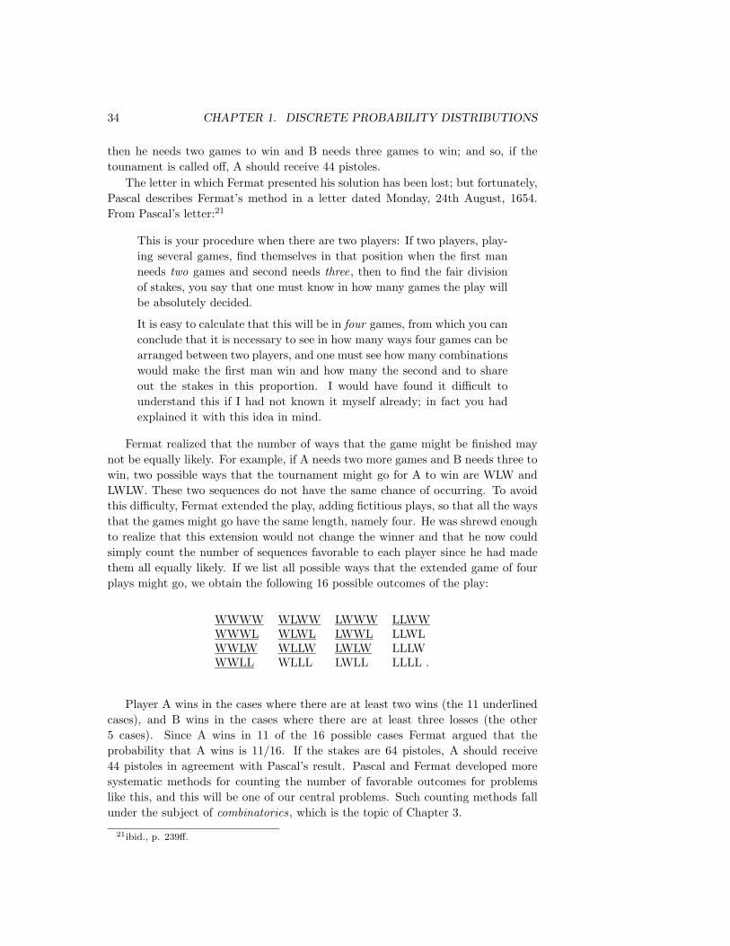
34 CHAPTER 1. DISCRETE PROBABILITY DISTRIBUTIONS
then he needs two games to win and B needs three games to win; and so, if thetounament is called off, A should receive 44 pistoles.
The letter in which Fermat presented his solution has been lost; but fortunately,Pascal describes Fermat’s method in a letter dated Monday, 24th August, 1654.From Pascal’s letter:21
This is your procedure when there are two players: If two players, play-ing several games, find themselves in that position when the first manneeds two games and second needs three, then to find the fair divisionof stakes, you say that one must know in how many games the play willbe absolutely decided.
It is easy to calculate that this will be in four games, from which you canconclude that it is necessary to see in how many ways four games can bearranged between two players, and one must see how many combinationswould make the first man win and how many the second and to shareout the stakes in this proportion. I would have found it difficult tounderstand this if I had not known it myself already; in fact you hadexplained it with this idea in mind.
Fermat realized that the number of ways that the game might be finished maynot be equally likely. For example, if A needs two more games and B needs three towin, two possible ways that the tournament might go for A to win are WLW andLWLW. These two sequences do not have the same chance of occurring. To avoidthis difficulty, Fermat extended the play, adding fictitious plays, so that all the waysthat the games might go have the same length, namely four. He was shrewd enoughto realize that this extension would not change the winner and that he now couldsimply count the number of sequences favorable to each player since he had madethem all equally likely. If we list all possible ways that the extended game of fourplays might go, we obtain the following 16 possible outcomes of the play:
WWWW WLWW LWWW LLWWWWWL WLWL LWWL LLWLWWLW WLLW LWLW LLLWWWLL WLLL LWLL LLLL .
Player A wins in the cases where there are at least two wins (the 11 underlinedcases), and B wins in the cases where there are at least three losses (the other5 cases). Since A wins in 11 of the 16 possible cases Fermat argued that theprobability that A wins is 11/16. If the stakes are 64 pistoles, A should receive44 pistoles in agreement with Pascal’s result. Pascal and Fermat developed moresystematic methods for counting the number of favorable outcomes for problemslike this, and this will be one of our central problems. Such counting methods fallunder the subject of combinatorics, which is the topic of Chapter 3.
21ibid., p. 239ff.

1.2. DISCRETE PROBABILITY DISTRIBUTIONS 35
We see that these two mathematicians arrived at two very different ways to solvethe problem of points. Pascal’s method was to develop an algorithm and use it tocalculate the fair division. This method is easy to implement on a computer and easyto generalize. Fermat’s method, on the other hand, was to change the problem intoan equivalent problem for which he could use counting or combinatorial methods.We will see in Chapter 3 that, in fact, Fermat used what has become known asPascal’s triangle! In our study of probability today we shall find that both thealgorithmic approach and the combinatorial approach share equal billing, just asthey did 300 years ago when probability got its start.
Exercises
1 Let Ω = a, b, c be a sample space. Let m(a) = 1/2, m(b) = 1/3, andm(c) = 1/6. Find the probabilities for all eight subsets of Ω.
2 Give a possible sample space Ω for each of the following experiments:
(a) An election decides between two candidates A and B.
(b) A two-sided coin is tossed.
(c) A student is asked for the month of the year and the day of the week onwhich her birthday falls.
(d) A student is chosen at random from a class of ten students.
(e) You receive a grade in this course.
3 For which of the cases in Exercise 2 would it be reasonable to assign theuniform distribution function?
4 Describe in words the events specified by the following subsets of
Ω = HHH, HHT, HTH, HTT, THH, THT, TTH, TTT
(see Example 1.6).
(a) E = HHH,HHT,HTH,HTT.(b) E = HHH,TTT.(c) E = HHT,HTH,THH.(d) E = HHT,HTH,HTT,THH,THT,TTH,TTT.
5 What are the probabilities of the events described in Exercise 4?
6 A die is loaded in such a way that the probability of each face turning upis proportional to the number of dots on that face. (For example, a six isthree times as probable as a two.) What is the probability of getting an evennumber in one throw?
7 Let A and B be events such that P (A ∩B) = 1/4, P (A) = 1/3, and P (B) =1/2. What is P (A ∪B)?

36 CHAPTER 1. DISCRETE PROBABILITY DISTRIBUTIONS
8 A student must choose one of the subjects, art, geology, or psychology, as anelective. She is equally likely to choose art or psychology and twice as likelyto choose geology. What are the respective probabilities that she chooses art,geology, and psychology?
9 A student must choose exactly two out of three electives: art, French, andmathematics. He chooses art with probability 5/8, French with probability5/8, and art and French together with probability 1/4. What is the probabilitythat he chooses mathematics? What is the probability that he chooses eitherart or French?
10 For a bill to come before the president of the United States, it must be passedby both the House of Representatives and the Senate. Assume that, of thebills presented to these two bodies, 60 percent pass the House, 80 percentpass the Senate, and 90 percent pass at least one of the two. Calculate theprobability that the next bill presented to the two groups will come before thepresident.
11 What odds should a person give in favor of the following events?
(a) A card chosen at random from a 52-card deck is an ace.
(b) Two heads will turn up when a coin is tossed twice.
(c) Boxcars (two sixes) will turn up when two dice are rolled.
12 You offer 3 : 1 odds that your friend Smith will be elected mayor of your city.What probability are you assigning to the event that Smith wins?
13 In a horse race, the odds that Romance will win are listed as 2 : 3 and thatDownhill will win are 1 : 2. What odds should be given for the event thateither Romance or Downhill wins?
14 Let X be a random variable with distribution function mX(x) defined by
mX(−1) = 1/5, mX(0) = 1/5, mX(1) = 2/5, mX(2) = 1/5 .
(a) Let Y be the random variable defined by the equation Y = X + 3. Findthe distribution function mY (y) of Y .
(b) Let Z be the random variable defined by the equation Z = X2. Find thedistribution function mZ(z) of Z.
*15 John and Mary are taking a mathematics course. The course has only threegrades: A, B, and C. The probability that John gets a B is .3. The probabilitythat Mary gets a B is .4. The probability that neither gets an A but at leastone gets a B is .1. What is the probability that at least one gets a B butneither gets a C?
16 In a fierce battle, not less than 70 percent of the soldiers lost one eye, not lessthan 75 percent lost one ear, not less than 80 percent lost one hand, and not

1.2. DISCRETE PROBABILITY DISTRIBUTIONS 37
less than 85 percent lost one leg. What is the minimal possible percentage ofthose who simultaneously lost one ear, one eye, one hand, and one leg?22
*17 Assume that the probability of a “success” on a single experiment with n
outcomes is 1/n. Let m be the number of experiments necessary to make it afavorable bet that at least one success will occur (see Exercise 1.1.5).
(a) Show that the probability that, in m trials, there are no successes is(1− 1/n)m.
(b) (de Moivre) Show that if m = n log 2 then
limn→∞
(1− 1
n
)m=
12.
Hint :
limn→∞
(1− 1
n
)n= e−1 .
Hence for large n we should choose m to be about n log 2.
(c) Would DeMoivre have been led to the correct answer for de Mere’s twobets if he had used his approximation?
18 (a) For events A1, . . . , An, prove that
P (A1 ∪ · · · ∪An) ≤ P (A1) + · · ·+ P (An) .
(b) For events A and B, prove that
P (A ∩B) ≥ P (A) + P (B)− 1.
19 If A, B, and C are any three events, show that
P (A ∪B ∪ C) = P (A) + P (B) + P (C)−P (A ∩B)− P (B ∩ C)− P (C ∩A)+P (A ∩B ∩ C) .
20 Explain why it is not possible to define a uniform distribution function (seeDefinition 1.3) on a countably infinite sample space. Hint : Assume m(ω) = a
for all ω, where 0 ≤ a ≤ 1. Does m(ω) have all the properties of a distributionfunction?
21 In Example 1.13 find the probability that the coin turns up heads for the firsttime on the tenth, eleventh, or twelfth toss.
22 A die is rolled until the first time that a six turns up. We shall see that theprobability that this occurs on the nth roll is (5/6)n−1 · (1/6). Using this fact,describe the appropriate infinite sample space and distribution function forthe experiment of rolling a die until a six turns up for the first time. Verifythat for your distribution function
∑ωm(ω) = 1.
22See Knot X, in Lewis Carroll, Mathematical Recreations, vol. 2 (Dover, 1958).

38 CHAPTER 1. DISCRETE PROBABILITY DISTRIBUTIONS
23 Let Ω be the sample space
Ω = 0, 1, 2, . . . ,
and define a distribution function by
m(j) = (1− r)jr ,
for some fixed r, 0 < r < 1, and for j = 0, 1, 2, . . .. Show that this is adistribution function for Ω.
24 Our calendar has a 400-year cycle. B. H. Brown noticed that the number oftimes the thirteenth of the month falls on each of the days of the week in the4800 months of a cycle is as follows:
Sunday 687
Monday 685
Tuesday 685
Wednesday 687
Thursday 684
Friday 688
Saturday 684
From this he deduced that the thirteenth was more likely to fall on Fridaythan on any other day. Explain what he meant by this.
25 Tversky and Kahneman23 asked a group of subjects to carry out the followingtask. They are told that:
Linda is 31, single, outspoken, and very bright. She majored inphilosophy in college. As a student, she was deeply concerned withracial discrimination and other social issues, and participated inanti-nuclear demonstrations.
The subjects are then asked to rank the likelihood of various alternatives, suchas:(1) Linda is active in the feminist movement.(2) Linda is a bank teller.(3) Linda is a bank teller and active in the feminist movement.
Tversky and Kahneman found that between 85 and 90 percent of the subjectsrated alternative (1) most likely, but alternative (3) more likely than alterna-tive (2). Is it? They call this phenomenon the conjunction fallacy, and notethat it appears to be unaffected by prior training in probability or statistics.Explain why this is a fallacy. Can you give a possible explanation for thesubjects’ choices?
23K. McKean, “Decisions, Decisions,” pp. 22–31.

1.2. DISCRETE PROBABILITY DISTRIBUTIONS 39
26 Two cards are drawn successively from a deck of 52 cards. Find the probabilitythat the second card is higher in rank than the first card. Hint : Show that 1 =P (higher) +P (lower) +P (same) and use the fact that P (higher) = P (lower).
27 A life table is a table that lists for a given number of births the estimatednumber of people who will live to a given age. In Appendix C we give a lifetable based upon 100,000 births for ages from 0 to 85, both for women and formen. Show how from this table you can estimate the probability m(x) that aperson born in 1981 would live to age x. Write a program to plot m(x) bothfor men and for women, and comment on the differences that you see in thetwo cases.
*28 Here is an attempt to get around the fact that we cannot choose a “randominteger.”
(a) What, intuitively, is the probability that a “randomly chosen” positiveinteger is a multiple of 3?
(b) Let P3(N) be the probability that an integer, chosen at random between1 and N , is a multiple of 3 (since the sample space is finite, this is alegitimate probability). Show that the limit
P3 = limN→∞
P3(N)
exists and equals 1/3. This formalizes the intuition in (a), and gives usa way to assign “probabilities” to certain events that are infinite subsetsof the positive integers.
(c) If A is any set of positive integers, let A(N) mean the number of elementsof A which are less than or equal to N . Then define the “probability” ofA as
P (A) = limN→∞
A(N)/N ,
provided this limit exists. Show that this definition would assign prob-ability 0 to any finite set and probability 1 to the set of all positiveintegers. Thus, the probability of the set of all integers is not the sum ofthe probabilities of the individual integers in this set. This means thatthe definition of probability given here is not a completely satisfactorydefinition.
(d) Let A be the set of all positive integers with an odd number of dig-its. Show that P (A) does not exist. This shows that under the abovedefinition of probability, not all sets have probabilities.
29 (from Sholander24) In a standard clover-leaf interchange, there are four rampsfor making right-hand turns, and inside these four ramps, there are four moreramps for making left-hand turns. Your car approaches the interchange fromthe south. A mechanism has been installed so that at each point where thereexists a choice of directions, the car turns to the right with fixed probability r.
24M. Sholander, Problem #1034, Mathematics Magazine, vol. 52, no. 3 (May 1979), p. 183.

40 CHAPTER 1. DISCRETE PROBABILITY DISTRIBUTIONS
(a) If r = 1/2, what is your chance of emerging from the interchange goingwest?
(b) Find the value of r that maximizes your chance of a westward departurefrom the interchange.
30 (from Benkoski25) Consider a “pure” cloverleaf interchange in which thereare no ramps for right-hand turns, but only the two intersecting straighthighways with cloverleaves for left-hand turns. (Thus, to turn right in suchan interchange, one must make three left-hand turns.) As in the precedingproblem, your car approaches the interchange from the south. What is thevalue of r that maximizes your chances of an eastward departure from theinterchange?
31 (from vos Savant26) A reader of Marilyn vos Savant’s column wrote in withthe following question:
My dad heard this story on the radio. At Duke University, twostudents had received A’s in chemistry all semester. But on thenight before the final exam, they were partying in another stateand didn’t get back to Duke until it was over. Their excuse to theprofessor was that they had a flat tire, and they asked if they couldtake a make-up test. The professor agreed, wrote out a test and sentthe two to separate rooms to take it. The first question (on one sideof the paper) was worth 5 points, and they answered it easily. Thenthey flipped the paper over and found the second question, worth95 points: ‘Which tire was it?’ What was the probability that bothstudents would say the same thing? My dad and I think it’s 1 in16. Is that right?”
(a) Is the answer 1/16?
(b) The following question was asked of a class of students. “I was drivingto school today, and one of my tires went flat. Which tire do you thinkit was?” The responses were as follows: right front, 58%, left front, 11%,right rear, 18%, left rear, 13%. Suppose that this distribution holds inthe general population, and assume that the two test-takers are randomlychosen from the general population. What is the probability that theywill give the same answer to the second question?
25S. Benkoski, Comment on Problem #1034, Mathematics Magazine, vol. 52, no. 3 (May 1979),pp. 183-184.
26M. vos Savant, Parade Magazine, 3 March 1996, p. 14.

Chapter 2
Continuous ProbabilityDensities
2.1 Simulation of Continuous Probabilities
In this section we shall show how we can use computer simulations for experimentsthat have a whole continuum of possible outcomes.
Probabilities
Example 2.1 We begin by constructing a spinner, which consists of a circle of unitcircumference and a pointer as shown in Figure 2.1. We pick a point on the circleand label it 0, and then label every other point on the circle with the distance, sayx, from 0 to that point, measured counterclockwise. The experiment consists ofspinning the pointer and recording the label of the point at the tip of the pointer.We let the random variable X denote the value of this outcome. The sample spaceis clearly the interval [0, 1). We would like to construct a probability model in whicheach outcome is equally likely to occur.
If we proceed as we did in Chapter 1 for experiments with a finite number ofpossible outcomes, then we must assign the probability 0 to each outcome, sinceotherwise, the sum of the probabilities, over all of the possible outcomes, wouldnot equal 1. (In fact, summing an uncountable number of real numbers is a trickybusiness; in particular, in order for such a sum to have any meaning, at mostcountably many of the summands can be different than 0.) However, if all of theassigned probabilities are 0, then the sum is 0, not 1, as it should be.
In the next section, we will show how to construct a probability model in thissituation. At present, we will assume that such a model can be constructed. Wewill also assume that in this model, if E is an arc of the circle, and E is of lengthp, then the model will assign the probability p to E. This means that if the pointeris spun, the probability that it ends up pointing to a point in E equals p, which iscertainly a reasonable thing to expect.
41

42 CHAPTER 2. CONTINUOUS PROBABILITY DENSITIES
0
x
Figure 2.1: A spinner.
To simulate this experiment on a computer is an easy matter. Many computersoftware packages have a function which returns a random real number in the in-terval [0, 1]. Actually, the returned value is always a rational number, and thevalues are determined by an algorithm, so a sequence of such values is not trulyrandom. Nevertheless, the sequences produced by such algorithms behave muchlike theoretically random sequences, so we can use such sequences in the simulationof experiments. On occasion, we will need to refer to such a function. We will callthis function rnd. 2
Monte Carlo Procedure and Areas
It is sometimes desirable to estimate quantities whose exact values are difficult orimpossible to calculate exactly. In some of these cases, a procedure involving chance,called a Monte Carlo procedure, can be used to provide such an estimate.
Example 2.2 In this example we show how simulation can be used to estimateareas of plane figures. Suppose that we program our computer to provide a pair(x, y) or numbers, each chosen independently at random from the interval [0, 1].Then we can interpret this pair (x, y) as the coordinates of a point chosen at randomfrom the unit square. Events are subsets of the unit square. Our experience withExample 2.1 suggests that the point is equally likely to fall in subsets of equal area.Since the total area of the square is 1, the probability of the point falling in a specificsubset E of the unit square should be equal to its area. Thus, we can estimate thearea of any subset of the unit square by estimating the probability that a pointchosen at random from this square falls in the subset.
We can use this method to estimate the area of the region E under the curvey = x2 in the unit square (see Figure 2.2). We choose a large number of points (x, y)at random and record what fraction of them fall in the region E = (x, y) : y ≤ x2 .
The program MonteCarlo will carry out this experiment for us. Running thisprogram for 10,000 experiments gives an estimate of .325 (see Figure 2.3).
From these experiments we would estimate the area to be about 1/3. Of course,

2.1. SIMULATION OF CONTINUOUS PROBABILITIES 43
1x
1
y
y = x2
E
Figure 2.2: Area under y = x2.
for this simple region we can find the exact area by calculus. In fact,
Area of E =∫ 1
0
x2 dx =13.
We have remarked in Chapter 1 that, when we simulate an experiment of this typen times to estimate a probability, we can expect the answer to be in error by atmost 1/
√n at least 95 percent of the time. For 10,000 experiments we can expect
an accuracy of 0.01, and our simulation did achieve this accuracy.This same argument works for any region E of the unit square. For example,
suppose E is the circle with center (1/2, 1/2) and radius 1/2. Then the probabilitythat our random point (x, y) lies inside the circle is equal to the area of the circle,that is,
P (E) = π(1
2
)2
=π
4.
If we did not know the value of π, we could estimate the value by performing thisexperiment a large number of times! 2
The above example is not the only way of estimating the value of π by a chanceexperiment. Here is another way, discovered by Buffon.1
1G. L. Buffon, in “Essai d’Arithmetique Morale,” Oeuvres Completes de Buffon avec Supple-ments, tome iv, ed. Dumenil (Paris, 1836).

44 CHAPTER 2. CONTINUOUS PROBABILITY DENSITIES
1
11000 trials
Estimate of area is .325
y = x2
E
Figure 2.3: Computing the area by simulation.
Buffon’s Needle
Example 2.3 Suppose that we take a card table and draw across the top surfacea set of parallel lines a unit distance apart. We then drop a common needle ofunit length at random on this surface and observe whether or not the needle liesacross one of the lines. We can describe the possible outcomes of this experimentby coordinates as follows: Let d be the distance from the center of the needle to thenearest line. Next, let L be the line determined by the needle, and define θ as theacute angle that the line L makes with the set of parallel lines. (The reader shouldcertainly be wary of this description of the sample space. We are attempting tocoordinatize a set of line segments. To see why one must be careful in the choiceof coordinates, see Example 2.6.) Using this description, we have 0 ≤ d ≤ 1/2, and0 ≤ θ ≤ π/2. Moreover, we see that the needle lies across the nearest line if andonly if the hypotenuse of the triangle (see Figure 2.4) is less than half the length ofthe needle, that is,
d
sin θ<
12.
Now we assume that when the needle drops, the pair (θ, d) is chosen at randomfrom the rectangle 0 ≤ θ ≤ π/2, 0 ≤ d ≤ 1/2. We observe whether the needle liesacross the nearest line (i.e., whether d ≤ (1/2) sin θ). The probability of this eventE is the fraction of the area of the rectangle which lies inside E (see Figure 2.5).

2.1. SIMULATION OF CONTINUOUS PROBABILITIES 45
d1/2
θ
Figure 2.4: Buffon’s experiment.
θ0
1/2
0
d
π/2
E
Figure 2.5: Set E of pairs (θ, d) with d < 12 sin θ.
Now the area of the rectangle is π/4, while the area of E is
Area =∫ π/2
0
12
sin θ dθ =12.
Hence, we get
P (E) =1/2π/4
=2π.
The program BuffonsNeedle simulates this experiment. In Figure 2.6, we showthe position of every 100th needle in a run of the program in which 10,000 needleswere “dropped.” Our final estimate for π is 3.139. While this was within 0.003 ofthe true value for π we had no right to expect such accuracy. The reason for thisis that our simulation estimates P (E). While we can expect this estimate to be inerror by at most 0.001, a small error in P (E) gets magnified when we use this tocompute π = 2/P (E). Perlman and Wichura, in their article “Sharpening Buffon’s

46 CHAPTER 2. CONTINUOUS PROBABILITY DENSITIES
0.00
5.00
0.50
1.00
1.50
2.00
2.50
3.00
3.50
4.00
4.50
5.0010000
3.139
Figure 2.6: Simulation of Buffon’s needle experiment.
Needle,”2 show that we can expect to have an error of not more than 5/√n about
95 percent of the time. Here n is the number of needles dropped. Thus for 10,000needles we should expect an error of no more than 0.05, and that was the case here.We see that a large number of experiments is necessary to get a decent estimate forπ. 2
In each of our examples so far, events of the same size are equally likely. Hereis an example where they are not. We will see many other such examples later.
Example 2.4 Suppose that we choose two random real numbers in [0, 1] and addthem together. Let X be the sum. How is X distributed?
To help understand the answer to this question, we can use the program Are-abargraph. This program produces a bar graph with the property that on eachinterval, the area, rather than the height, of the bar is equal to the fraction of out-comes that fell in the corresponding interval. We have carried out this experiment1000 times; the data is shown in Figure 2.7. It appears that the function definedby
f(x) =x, if 0 ≤ x ≤ 1,2− x, if 1 < x ≤ 2
fits the data very well. (It is shown in the figure.) In the next section, we willsee that this function is the “right” function. By this we mean that if a and b areany two real numbers between 0 and 2, with a ≤ b, then we can use this functionto calculate the probability that a ≤ X ≤ b. To understand how this calculationmight be performed, we again consider Figure 2.7. Because of the way the barswere constructed, the sum of the areas of the bars corresponding to the interval
2M. D. Perlman and M. J. Wichura, “Sharpening Buffon’s Needle,” The American Statistician,vol. 29, no. 4 (1975), pp. 157–163.

2.1. SIMULATION OF CONTINUOUS PROBABILITIES 47
0 0.5 1 1.5 20
0.2
0.4
0.6
0.8
1
Figure 2.7: Sum of two random numbers.
[a, b] approximates the probability that a ≤ X ≤ b. But the sum of the areas ofthese bars also approximates the integral∫ b
a
f(x) dx .
This suggests that for an experiment with a continuum of possible outcomes, if wefind a function with the above property, then we will be able to use it to calculateprobabilities. In the next section, we will show how to determine the functionf(x). 2
Example 2.5 Suppose that we choose 100 random numbers in [0, 1], and let Xrepresent their sum. How is X distributed? We have carried out this experiment10000 times; the results are shown in Figure 2.8. It is not so clear what functionfits the bars in this case. It turns out that the type of function which does the jobis called a normal density function. This type of function is sometimes referred toas a “bell-shaped” curve. It is among the most important functions in the subjectof probability, and will be formally defined in Section 5.2 of Chapter 4.3. 2
Our last example explores the fundamental question of how probabilities areassigned.
Bertrand’s Paradox
Example 2.6 A chord of a circle is a line segment both of whose endpoints lie onthe circle. Suppose that a chord is drawn at random in a unit circle. What is theprobability that its length exceeds
√3?
Our answer will depend on what we mean by random, which will depend, in turn,on what we choose for coordinates. The sample space Ω is the set of all possiblechords in the circle. To find coordinates for these chords, we first introduce a

48 CHAPTER 2. CONTINUOUS PROBABILITY DENSITIES
40 45 50 55 600
0.02
0.04
0.06
0.08
0.1
0.12
0.14
Figure 2.8: Sum of 100 random numbers.
x
y
A
B
M
θβ
α
Figure 2.9: Random chord.
rectangular coordinate system with origin at the center of the circle (see Figure 2.9).We note that a chord of a circle is perpendicular to the radial line containing themidpoint of the chord. We can describe each chord by giving:
1. The rectangular coordinates (x, y) of the midpoint M , or
2. The polar coordinates (r, θ) of the midpoint M , or
3. The polar coordinates (1, α) and (1, β) of the endpoints A and B.
In each case we shall interpret at random to mean: choose these coordinates atrandom.
We can easily estimate this probability by computer simulation. In programmingthis simulation, it is convenient to include certain simplifications, which we describein turn:

2.1. SIMULATION OF CONTINUOUS PROBABILITIES 49
1. To simulate this case, we choose values for x and y from [−1, 1] at random.Then we check whether x2 + y2 ≤ 1. If not, the point M = (x, y) lies outsidethe circle and cannot be the midpoint of any chord, and we ignore it. Oth-erwise, M lies inside the circle and is the midpoint of a unique chord, whoselength L is given by the formula:
L = 2√
1− (x2 + y2) .
2. To simulate this case, we take account of the fact that any rotation of thecircle does not change the length of the chord, so we might as well assume inadvance that the chord is horizontal. Then we choose r from [−1, 1] at random,and compute the length of the resulting chord with midpoint (r, π/2) by theformula:
L = 2√
1− r2 .
3. To simulate this case, we assume that one endpoint, say B, lies at (1, 0) (i.e.,that β = 0). Then we choose a value for α from [0, 2π] at random and computethe length of the resulting chord, using the Law of Cosines, by the formula:
L =√
2− 2 cosα .
The program BertrandsParadox carries out this simulation. Running thisprogram produces the results shown in Figure 2.10. In the first circle in this figure,a smaller circle has been drawn. Those chords which intersect this smaller circlehave length at least
√3. In the second circle in the figure, the vertical line intersects
all chords of length at least√
3. In the third circle, again the vertical line intersectsall chords of length at least
√3.
In each case we run the experiment a large number of times and record thefraction of these lengths that exceed
√3. We have printed the results of every
100th trial up to 10,000 trials.It is interesting to observe that these fractions are not the same in the three cases;
they depend on our choice of coordinates. This phenomenon was first observed byBertrand, and is now known as Bertrand’s paradox.3 It is actually not a paradox atall; it is merely a reflection of the fact that different choices of coordinates will leadto different assignments of probabilities. Which assignment is “correct” depends onwhat application or interpretation of the model one has in mind.
One can imagine a real experiment involving throwing long straws at a circledrawn on a card table. A “correct” assignment of coordinates should not dependon where the circle lies on the card table, or where the card table sits in the room.Jaynes4 has shown that the only assignment which meets this requirement is (2).In this sense, the assignment (2) is the natural, or “correct” one (see Exercise 11).
We can easily see in each case what the true probabilities are if we note that√3 is the length of the side of an inscribed equilateral triangle. Hence, a chord has3J. Bertrand, Calcul des Probabilites (Paris: Gauthier-Villars, 1889).4E. T. Jaynes, “The Well-Posed Problem,” in Papers on Probability, Statistics and Statistical
Physics, R. D. Rosencrantz, ed. (Dordrecht: D. Reidel, 1983), pp. 133–148.

50 CHAPTER 2. CONTINUOUS PROBABILITY DENSITIES
.0
1.0
.2
.4
.6
.8
1.0
.488
.227
.0
1.0
.2
.4
.6
.8
1.0
.0
1.0
.2
.4
.6
.8
1.0
.332
10000 10000 10000
Figure 2.10: Bertrand’s paradox.
length L >√
3 if its midpoint has distance d < 1/2 from the origin (see Figure 2.9).The following calculations determine the probability that L >
√3 in each of the
three cases.
1. L >√
3 if(x, y) lies inside a circle of radius 1/2, which occurs with probability
p =π(1/2)2
π(1)2=
14.
2. L >√
3 if |r| < 1/2, which occurs with probability
1/2− (−1/2)1− (−1)
=12.
3. L >√
3 if 2π/3 < α < 4π/3, which occurs with probability
4π/3− 2π/32π − 0
=13.
We see that our simulations agree quite well with these theoretical values. 2
Historical Remarks
G. L. Buffon (1707–1788) was a natural scientist in the eighteenth century whoapplied probability to a number of his investigations. His work is found in hismonumental 44-volume Histoire Naturelle and its supplements.5 For example, he
5G. L. Buffon, Histoire Naturelle, Generali et Particular avec le Description du Cabinet duRoy, 44 vols. (Paris: L‘Imprimerie Royale, 1749–1803).

2.1. SIMULATION OF CONTINUOUS PROBABILITIES 51
Length of Number of Number of EstimateExperimenter needle casts crossings for πWolf, 1850 .8 5000 2532 3.1596Smith, 1855 .6 3204 1218.5 3.1553De Morgan, c.1860 1.0 600 382.5 3.137Fox, 1864 .75 1030 489 3.1595Lazzerini, 1901 .83 3408 1808 3.1415929Reina, 1925 .5419 2520 869 3.1795
Table 2.1: Buffon needle experiments to estimate π.
presented a number of mortality tables and used them to compute, for each agegroup, the expected remaining lifetime. From his table he observed: the expectedremaining lifetime of an infant of one year is 33 years, while that of a man of 21years is also approximately 33 years. Thus, a father who is not yet 21 can hope tolive longer than his one year old son, but if the father is 40, the odds are already 3to 2 that his son will outlive him.6
Buffon wanted to show that not all probability calculations rely only on algebra,but that some rely on geometrical calculations. One such problem was his famous“needle problem” as discussed in this chapter.7 In his original formulation, Buffondescribes a game in which two gamblers drop a loaf of French bread on a wide-boardfloor and bet on whether or not the loaf falls across a crack in the floor. Buffonasked: what length L should the bread loaf be, relative to the width W of thefloorboards, so that the game is fair. He found the correct answer (L = (π/4)W )using essentially the methods described in this chapter. He also considered the caseof a checkerboard floor, but gave the wrong answer in this case. The correct answerwas given later by Laplace.
The literature contains descriptions of a number of experiments that were actu-ally carried out to estimate π by this method of dropping needles. N. T. Gridgeman8
discusses the experiments shown in Table 2.1. (The halves for the number of cross-ing comes from a compromise when it could not be decided if a crossing had actuallyoccurred.) He observes, as we have, that 10,000 casts could do no more than estab-lish the first decimal place of π with reasonable confidence. Gridgeman points outthat, although none of the experiments used even 10,000 casts, they are surprisinglygood, and in some cases, too good. The fact that the number of casts is not alwaysa round number would suggest that the authors might have resorted to clever stop-ping to get a good answer. Gridgeman comments that Lazzerini’s estimate turnedout to agree with a well-known approximation to π, 355/113 = 3.1415929, discov-ered by the fifth-century Chinese mathematician, Tsu Ch’ungchih. Gridgeman saysthat he did not have Lazzerini’s original report, and while waiting for it (knowing
6G. L. Buffon, “Essai d’Arithmetique Morale,” p. 301.7ibid., pp. 277–278.8N. T. Gridgeman, “Geometric Probability and the Number π” Scripta Mathematika, vol. 25,
no. 3, (1960), pp. 183–195.

52 CHAPTER 2. CONTINUOUS PROBABILITY DENSITIES
only the needle crossed a line 1808 times in 3408 casts) deduced that the length ofthe needle must have been 5/6. He calculated this from Buffon’s formula, assumingπ = 355/113:
L =πP (E)
2=
12
(355113
)(18083408
)=
56
= .8333 .
Even with careful planning one would have to be extremely lucky to be able to stopso cleverly.
The second author likes to trace his interest in probability theory to the ChicagoWorld’s Fair of 1933 where he observed a mechanical device dropping needles anddisplaying the ever-changing estimates for the value of π. (The first author likes totrace his interest in probability theory to the second author.)
Exercises
*1 In the spinner problem (see Example 2.1) divide the unit circumference intothree arcs of length 1/2, 1/3, and 1/6. Write a program to simulate thespinner experiment 1000 times and print out what fraction of the outcomesfall in each of the three arcs. Now plot a bar graph whose bars have width 1/2,1/3, and 1/6, and areas equal to the corresponding fractions as determinedby your simulation. Show that the heights of the bars are all nearly the same.
2 Do the same as in Exercise 1, but divide the unit circumference into five arcsof length 1/3, 1/4, 1/5, 1/6, and 1/20.
3 Alter the program MonteCarlo to estimate the area of the circle of radius1/2 with center at (1/2, 1/2) inside the unit square by choosing 1000 pointsat random. Compare your results with the true value of π/4. Use your resultsto estimate the value of π. How accurate is your estimate?
4 Alter the program MonteCarlo to estimate the area under the graph ofy = sinπx inside the unit square by choosing 10,000 points at random. Nowcalculate the true value of this area and use your results to estimate the valueof π. How accurate is your estimate?
5 Alter the program MonteCarlo to estimate the area under the graph ofy = 1/(x+ 1) in the unit square in the same way as in Exercise 4. Calculatethe true value of this area and use your simulation results to estimate thevalue of log 2. How accurate is your estimate?
6 To simulate the Buffon’s needle problem we choose independently the dis-tance d and the angle θ at random, with 0 ≤ d ≤ 1/2 and 0 ≤ θ ≤ π/2,and check whether d ≤ (1/2) sin θ. Doing this a large number of times, weestimate π as 2/a, where a is the fraction of the times that d ≤ (1/2) sin θ.Write a program to estimate π by this method. Run your program severaltimes for each of 100, 1000, and 10,000 experiments. Does the accuracy ofthe experimental approximation for π improve as the number of experimentsincreases?

2.1. SIMULATION OF CONTINUOUS PROBABILITIES 53
7 For Buffon’s needle problem, Laplace9 considered a grid with horizontal andvertical lines one unit apart. He showed that the probability that a needle oflength L ≤ 1 crosses at least one line is
p =4L− L2
π.
To simulate this experiment we choose at random an angle θ between 0 andπ/2 and independently two numbers d1 and d2 between 0 and L/2. (The twonumbers represent the distance from the center of the needle to the nearesthorizontal and vertical line.) The needle crosses a line if either d1 ≤ (L/2) sin θor d2 ≤ (L/2) cos θ. We do this a large number of times and estimate π as
π =4L− L2
a,
where a is the proportion of times that the needle crosses at least one line.Write a program to estimate π by this method, run your program for 100,1000, and 10,000 experiments, and compare your results with Buffon’s methoddescribed in Exercise 6. (Take L = 1.)
8 A long needle of length L much bigger than 1 is dropped on a grid withhorizontal and vertical lines one unit apart. We will see (in Exercise 6.3.28)that the average number a of lines crossed is approximately
a =4Lπ
.
To estimate π by simulation, pick an angle θ at random between 0 and π/2 andcompute L sin θ + L cos θ. This may be used for the number of lines crossed.Repeat this many times and estimate π by
π =4La
,
where a is the average number of lines crossed per experiment. Write a pro-gram to simulate this experiment and run your program for the number ofexperiments equal to 100, 1000, and 10,000. Compare your results with themethods of Laplace or Buffon for the same number of experiments. (UseL = 100.)
The following exercises involve experiments in which not all outcomes areequally likely. We shall consider such experiments in detail in the next section,but we invite you to explore a few simple cases here.
9 A large number of waiting time problems have an exponential distribution ofoutcomes. We shall see (in Section 5.2) that such outcomes are simulated bycomputing (−1/λ) log(rnd), where λ > 0. For waiting times produced in thisway, the average waiting time is 1/λ. For example, the times spent waiting for
9P. S. Laplace, Theorie Analytique des Probabilites (Paris: Courcier, 1812).

54 CHAPTER 2. CONTINUOUS PROBABILITY DENSITIES
a car to pass on a highway, or the times between emissions of particles from aradioactive source, are simulated by a sequence of random numbers, each ofwhich is chosen by computing (−1/λ) log(rnd), where 1/λ is the average timebetween cars or emissions. Write a program to simulate the times betweencars when the average time between cars is 30 seconds. Have your programcompute an area bar graph for these times by breaking the time interval from0 to 120 into 24 subintervals. On the same pair of axes, plot the functionf(x) = (1/30)e−(1/30)x. Does the function fit the bar graph well?
10 In Exercise 9, the distribution came “out of a hat.” In this problem, we willagain consider an experiment whose outcomes are not equally likely. We willdetermine a function f(x) which can be used to determine the probability ofcertain events. Let T be the right triangle in the plane with vertices at thepoints (0, 0), (1, 0), and (0, 1). The experiment consists of picking a pointat random in the interior of T , and recording only the x-coordinate of thepoint. Thus, the sample space is the set [0, 1], but the outcomes do not seemto be equally likely. We can simulate this experiment by asking a computer toreturn two random real numbers in [0, 1], and recording the first of these twonumbers if their sum is less than 1. Write this program and run it for 10,000trials. Then make a bar graph of the result, breaking the interval [0, 1] into10 intervals. Compare the bar graph with the function f(x) = 2 − 2x. Nowshow that there is a constant c such that the height of T at the x-coordinatevalue x is c times f(x) for every x in [0, 1]. Finally, show that∫ 1
0
f(x) dx = 1 .
How might one use the function f(x) to determine the probability that theoutcome is between .2 and .5?
11 Here is another way to pick a chord at random on the circle of unit radius.Imagine that we have a card table whose sides are of length 100. We placecoordinate axes on the table in such a way that each side of the table is parallelto one of the axes, and so that the center of the table is the origin. We nowplace a circle of unit radius on the table so that the center of the circle is theorigin. Now pick out a point (x0, y0) at random in the square, and an angle θat random in the interval (−π/2, π/2). Let m = tan θ. Then the equation ofthe line passing through (x0, y0) with slope m is
y = y0 +m(x− x0) ,
and the distance of this line from the center of the circle (i.e., the origin) is
d =∣∣∣∣y0 −mx0√
m2 + 1
∣∣∣∣ .We can use this distance formula to check whether the line intersects the circle(i.e., whether d < 1). If so, we consider the resulting chord a random chord.

2.2. CONTINUOUS DENSITY FUNCTIONS 55
This describes an experiment of dropping a long straw at random on a tableon which a circle is drawn.
Write a program to simulate this experiment 10000 times and estimate theprobability that the length of the chord is greater than
√3. How does your
estimate compare with the results of Example 2.6?
2.2 Continuous Density Functions
In the previous section we have seen how to simulate experiments with a wholecontinuum of possible outcomes and have gained some experience in thinking aboutsuch experiments. Now we turn to the general problem of assigning probabilities tothe outcomes and events in such experiments. We shall restrict our attention hereto those experiments whose sample space can be taken as a suitably chosen subsetof the line, the plane, or some other Euclidean space. We begin with some simpleexamples.
Spinners
Example 2.7 The spinner experiment described in Example 2.1 has the interval[0, 1) as the set of possible outcomes. We would like to construct a probabilitymodel in which each outcome is equally likely to occur. We saw that in such amodel, it is necessary to assign the probability 0 to each outcome. This does not atall mean that the probability of every event must be zero. On the contrary, if welet the random variable X denote the outcome, then the probability
P ( 0 ≤ X ≤ 1)
that the head of the spinner comes to rest somewhere in the circle, should be equalto 1. Also, the probability that it comes to rest in the upper half of the circle shouldbe the same as for the lower half, so that
P
(0 ≤ X <
12
)= P
(12≤ X < 1
)=
12.
More generally, in our model, we would like the equation
P (c ≤ X < d) = d− c
to be true for every choice of c and d.If we let E = [c, d], then we can write the above formula in the form
P (E) =∫E
f(x) dx ,
where f(x) is the constant function with value 1. This should remind the reader ofthe corresponding formula in the discrete case for the probability of an event:
P (E) =∑ω∈E
m(ω) .

56 CHAPTER 2. CONTINUOUS PROBABILITY DENSITIES
0 0.2 0.4 0.6 0.8 1
0
0.2
0.4
0.6
0.8
1
Figure 2.11: Spinner experiment.
The difference is that in the continuous case, the quantity being integrated, f(x),is not the probability of the outcome x. (However, if one uses infinitesimals, onecan consider f(x) dx as the probability of the outcome x.)
In the continuous case, we will use the following convention. If the set of out-comes is a set of real numbers, then the individual outcomes will be referred toby small Roman letters such as x. If the set of outcomes is a subset of R2, thenthe individual outcomes will be denoted by (x, y). In either case, it may be moreconvenient to refer to an individual outcome by using ω, as in Chapter 1.
Figure 2.11 shows the results of 1000 spins of the spinner. The function f(x)is also shown in the figure. The reader will note that the area under f(x) andabove a given interval is approximately equal to the fraction of outcomes that fellin that interval. The function f(x) is called the density function of the randomvariable X. The fact that the area under f(x) and above an interval correspondsto a probability is the defining property of density functions. A precise definitionof density functions will be given shortly. 2
Darts
Example 2.8 A game of darts involves throwing a dart at a circular target of unitradius. Suppose we throw a dart once so that it hits the target, and we observewhere it lands.
To describe the possible outcomes of this experiment, it is natural to take as oursample space the set Ω of all the points in the target. It is convenient to describethese points by their rectangular coordinates, relative to a coordinate system withorigin at the center of the target, so that each pair (x, y) of coordinates with x2+y2 ≤1 describes a possible outcome of the experiment. Then Ω = (x, y) : x2 + y2 ≤ 1 is a subset of the Euclidean plane, and the event E = (x, y) : y > 0 , for example,corresponds to the statement that the dart lands in the upper half of the target,and so forth. Unless there is reason to believe otherwise (and with experts at the

2.2. CONTINUOUS DENSITY FUNCTIONS 57
game there may well be!), it is natural to assume that the coordinates are chosenat random. (When doing this with a computer, each coordinate is chosen uniformlyfrom the interval [−1, 1]. If the resulting point does not lie inside the unit circle,the point is not counted.) Then the arguments used in the preceding example showthat the probability of any elementary event, consisting of a single outcome, mustbe zero, and suggest that the probability of the event that the dart lands in anysubset E of the target should be determined by what fraction of the target area liesin E. Thus,
P (E) =area of E
area of target=
area of Eπ
.
This can be written in the form
P (E) =∫E
f(x) dx ,
where f(x) is the constant function with value 1/π. In particular, if E = (x, y) :x2 + y2 ≤ a2 is the event that the dart lands within distance a < 1 of the centerof the target, then
P (E) =πa2
π= a2 .
For example, the probability that the dart lies within a distance 1/2 of the centeris 1/4. 2
Example 2.9 In the dart game considered above, suppose that, instead of observ-ing where the dart lands, we observe how far it lands from the center of the target.
In this case, we take as our sample space the set Ω of all circles with centers atthe center of the target. It is convenient to describe these circles by their radii, sothat each circle is identified by its radius r, 0 ≤ r ≤ 1. In this way, we may regardΩ as the subset [0, 1] of the real line.
What probabilities should we assign to the events E of Ω? If
E = r : 0 ≤ r ≤ a ,
then E occurs if the dart lands within a distance a of the center, that is, within thecircle of radius a, and we saw in the previous example that under our assumptionsthe probability of this event is given by
P ([0, a]) = a2 .
More generally, ifE = r : a ≤ r ≤ b ,
then by our basic assumptions,
P (E) = P ([a, b]) = P ([0, b])− P ([0, a])
= b2 − a2
= (b− a)(b+ a)
= 2(b− a)(b+ a)
2.
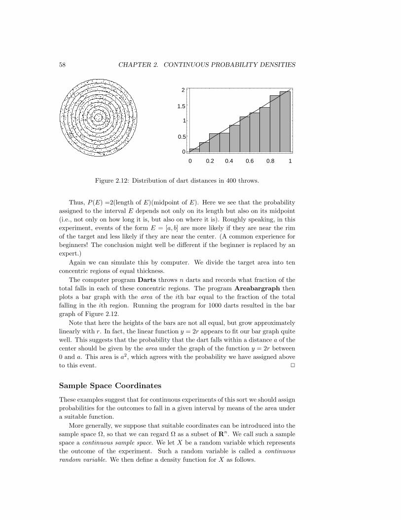
58 CHAPTER 2. CONTINUOUS PROBABILITY DENSITIES
0 0.2 0.4 0.6 0.8 1
0
0.5
1
1.5
2
0 0.2 0.4 0.6 0.8 1
2
1.5
1
0.5
0
Figure 2.12: Distribution of dart distances in 400 throws.
Thus, P (E) =2(length of E)(midpoint of E). Here we see that the probabilityassigned to the interval E depends not only on its length but also on its midpoint(i.e., not only on how long it is, but also on where it is). Roughly speaking, in thisexperiment, events of the form E = [a, b] are more likely if they are near the rimof the target and less likely if they are near the center. (A common experience forbeginners! The conclusion might well be different if the beginner is replaced by anexpert.)
Again we can simulate this by computer. We divide the target area into tenconcentric regions of equal thickness.
The computer program Darts throws n darts and records what fraction of thetotal falls in each of these concentric regions. The program Areabargraph thenplots a bar graph with the area of the ith bar equal to the fraction of the totalfalling in the ith region. Running the program for 1000 darts resulted in the bargraph of Figure 2.12.
Note that here the heights of the bars are not all equal, but grow approximatelylinearly with r. In fact, the linear function y = 2r appears to fit our bar graph quitewell. This suggests that the probability that the dart falls within a distance a of thecenter should be given by the area under the graph of the function y = 2r between0 and a. This area is a2, which agrees with the probability we have assigned aboveto this event. 2
Sample Space Coordinates
These examples suggest that for continuous experiments of this sort we should assignprobabilities for the outcomes to fall in a given interval by means of the area undera suitable function.
More generally, we suppose that suitable coordinates can be introduced into thesample space Ω, so that we can regard Ω as a subset of Rn. We call such a samplespace a continuous sample space. We let X be a random variable which representsthe outcome of the experiment. Such a random variable is called a continuousrandom variable. We then define a density function for X as follows.

2.2. CONTINUOUS DENSITY FUNCTIONS 59
Density Functions of Continuous Random Variables
Definition 2.1 Let X be a continuous real-valued random variable. A densityfunction for X is a real-valued function f which satisfies
P (a ≤ X ≤ b) =∫ b
a
f(x) dx
for all a, b ∈ R. 2
We note that it is not the case that all continuous real-valued random variablespossess density functions. However, in this book, we will only consider continuousrandom variables for which density functions exist.
In terms of the density f(x), if E is a subset of R, then
P (X ∈ E) =∫E
f(x) dx .
The notation here assumes that E is a subset of R for which∫Ef(x) dx makes
sense.
Example 2.10 (Example 2.7 continued) In the spinner experiment, we choose forour set of outcomes the interval 0 ≤ x < 1, and for our density function
f(x) =
1, if 0 ≤ x < 1,0, otherwise.
If E is the event that the head of the spinner falls in the upper half of the circle,then E = x : 0 ≤ x ≤ 1/2 , and so
P (E) =∫ 1/2
0
1 dx =12.
More generally, if E is the event that the head falls in the interval [a, b], then
P (E) =∫ b
a
1 dx = b− a .
2
Example 2.11 (Example 2.8 continued) In the first dart game experiment, wechoose for our sample space a disc of unit radius in the plane and for our densityfunction the function
f(x, y) =
1/π, if x2 + y2 ≤ 1,0, otherwise.
The probability that the dart lands inside the subset E is then given by
P (E) =∫ ∫
E
1πdx dy
=1π· (area of E) .
2
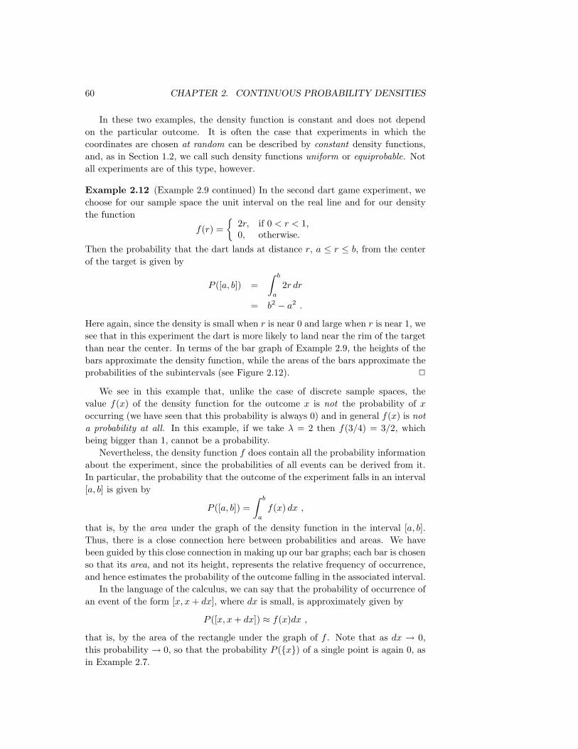
60 CHAPTER 2. CONTINUOUS PROBABILITY DENSITIES
In these two examples, the density function is constant and does not dependon the particular outcome. It is often the case that experiments in which thecoordinates are chosen at random can be described by constant density functions,and, as in Section 1.2, we call such density functions uniform or equiprobable. Notall experiments are of this type, however.
Example 2.12 (Example 2.9 continued) In the second dart game experiment, wechoose for our sample space the unit interval on the real line and for our densitythe function
f(r) =
2r, if 0 < r < 1,0, otherwise.
Then the probability that the dart lands at distance r, a ≤ r ≤ b, from the centerof the target is given by
P ([a, b]) =∫ b
a
2r dr
= b2 − a2 .
Here again, since the density is small when r is near 0 and large when r is near 1, wesee that in this experiment the dart is more likely to land near the rim of the targetthan near the center. In terms of the bar graph of Example 2.9, the heights of thebars approximate the density function, while the areas of the bars approximate theprobabilities of the subintervals (see Figure 2.12). 2
We see in this example that, unlike the case of discrete sample spaces, thevalue f(x) of the density function for the outcome x is not the probability of xoccurring (we have seen that this probability is always 0) and in general f(x) is nota probability at all. In this example, if we take λ = 2 then f(3/4) = 3/2, whichbeing bigger than 1, cannot be a probability.
Nevertheless, the density function f does contain all the probability informationabout the experiment, since the probabilities of all events can be derived from it.In particular, the probability that the outcome of the experiment falls in an interval[a, b] is given by
P ([a, b]) =∫ b
a
f(x) dx ,
that is, by the area under the graph of the density function in the interval [a, b].Thus, there is a close connection here between probabilities and areas. We havebeen guided by this close connection in making up our bar graphs; each bar is chosenso that its area, and not its height, represents the relative frequency of occurrence,and hence estimates the probability of the outcome falling in the associated interval.
In the language of the calculus, we can say that the probability of occurrence ofan event of the form [x, x+ dx], where dx is small, is approximately given by
P ([x, x+ dx]) ≈ f(x)dx ,
that is, by the area of the rectangle under the graph of f . Note that as dx → 0,this probability → 0, so that the probability P (x) of a single point is again 0, asin Example 2.7.

2.2. CONTINUOUS DENSITY FUNCTIONS 61
A glance at the graph of a density function tells us immediately which events ofan experiment are more likely. Roughly speaking, we can say that where the densityis large the events are more likely, and where it is small the events are less likely.In Example 2.4 the density function is largest at 1. Thus, given the two intervals[0, a] and [1, 1 + a], where a is a small positive real number, we see that X is morelikely to take on a value in the second interval than in the first.
Cumulative Distribution Functions of Continuous RandomVariables
We have seen that density functions are useful when considering continuous ran-dom variables. There is another kind of function, closely related to these densityfunctions, which is also of great importance. These functions are called cumulativedistribution functions.
Definition 2.2 Let X be a continuous real-valued random variable. Then thecumulative distribution function of X is defined by the equation
FX(x) = P (X ≤ x) .
2
If X is a continuous real-valued random variable which possesses a density function,then it also has a cumulative distribution function, and the following theorem showsthat the two functions are related in a very nice way.
Theorem 2.1 Let X be a continuous real-valued random variable with densityfunction f(x). Then the function defined by
F (x) =∫ x
−∞f(t) dt
is the cumulative distribution function of X. Furthermore, we have
d
dxF (x) = f(x) .
Proof. By definition,F (x) = P (X ≤ x) .
Let E = (−∞, x]. ThenP (X ≤ x) = P (X ∈ E) ,
which equals ∫ x
−∞f(t) dt .
Applying the Fundamental Theorem of Calculus to the first equation in thestatement of the theorem yields the second statement. 2

62 CHAPTER 2. CONTINUOUS PROBABILITY DENSITIES
-1 -0.5 0 0.5 1 1.5 2
0.25
0.5
0.75
1
1.25
1.5
1.75
2
f (x)
F (x)
X
X
Figure 2.13: Distribution and density for X = U2.
In many experiments, the density function of the relevant random variable is easyto write down. However, it is quite often the case that the cumulative distributionfunction is easier to obtain than the density function. (Of course, once we havethe cumulative distribution function, the density function can easily be obtained bydifferentiation, as the above theorem shows.) We now give some examples whichexhibit this phenomenon.
Example 2.13 A real number is chosen at random from [0, 1] with uniform prob-ability, and then this number is squared. Let X represent the result. What is thecumulative distribution function of X? What is the density of X?
We begin by letting U represent the chosen real number. Then X = U2. If0 ≤ x ≤ 1, then we have
FX(x) = P (X ≤ x)
= P (U2 ≤ x)
= P (U ≤√x)
=√x .
It is clear that X always takes on a value between 0 and 1, so the cumulativedistribution function of X is given by
FX(x) =
0, if x ≤ 0,√x, if 0 ≤ x ≤ 1,
1, if x ≥ 1.
From this we easily calculate that the density function of X is
fX(x) =
0, if x ≤ 0,1/(2√x), if 0 ≤ x ≤ 1,
0, if x > 1.
Note that FX(x) is continuous, but fX(x) is not. (See Figure 2.13.) 2

2.2. CONTINUOUS DENSITY FUNCTIONS 63
0.2 0.4 0.6 0.8 1
0.2
0.4
0.6
0.8
1
E.8
Figure 2.14: Calculation of distribution function for Example 2.14.
When referring to a continuous random variable X (say with a uniform densityfunction), it is customary to say that “X is uniformly distributed on the interval[a, b].” It is also customary to refer to the cumulative distribution function of X asthe distribution function of X. Thus, the word “distribution” is being used in sev-eral different ways in the subject of probability. (Recall that it also has a meaningwhen discussing discrete random variables.) When referring to the cumulative dis-tribution function of a continuous random variable X, we will always use the word“cumulative” as a modifier, unless the use of another modifier, such as “normal” or“exponential,” makes it clear. Since the phrase “uniformly densitied on the interval[a, b]” is not acceptable English, we will have to say “uniformly distributed” instead.
Example 2.14 In Example 2.4, we considered a random variable, defined to bethe sum of two random real numbers chosen uniformly from [0, 1]. Let the randomvariables X and Y denote the two chosen real numbers. Define Z = X + Y . Wewill now derive expressions for the cumulative distribution function and the densityfunction of Z.
Here we take for our sample space Ω the unit square in R2 with uniform density.A point ω ∈ Ω then consists of a pair (x, y) of numbers chosen at random. Then0 ≤ Z ≤ 2. Let Ez denote the event that Z ≤ z. In Figure 2.14, we show the setE.8. The event Ez, for any z between 0 and 1, looks very similar to the shaded setin the figure. For 1 < z ≤ 2, the set Ez looks like the unit square with a triangleremoved from the upper right-hand corner. We can now calculate the probabilitydistribution FZ of Z; it is given by
FZ(z) = P (Z ≤ z)= Area of Ez

64 CHAPTER 2. CONTINUOUS PROBABILITY DENSITIES
-1 1 2 3
0.2
0.4
0.6
0.8
1
-1 1 2 3
0.2
0.4
0.6
0.8
1
FZ (z)
f (z)Z
Figure 2.15: Distribution and density functions for Example 2.14.
1
E
Z
Figure 2.16: Calculation of Fz for Example 2.15.
=
0, if z < 0,(1/2)z2, if 0 ≤ z ≤ 1,1− (1/2)(2− z)2, if 1 ≤ z ≤ 2,1, if 2 < z.
The density function is obtained by differentiating this function:
fZ(z) =
0, if z < 0,z, if 0 ≤ z ≤ 1,2− z, if 1 ≤ z ≤ 2,0, if 2 < z.
The reader is referred to Figure 2.15 for the graphs of these functions. 2
Example 2.15 In the dart game described in Example 2.8, what is the distributionof the distance of the dart from the center of the target? What is its density?
Here, as before, our sample space Ω is the unit disk in R2, with coordinates(X,Y ). Let Z =
√X2 + Y 2 represent the distance from the center of the target. Let

2.2. CONTINUOUS DENSITY FUNCTIONS 65
-1 -0.5 0.5 1 1.5 2
0.2
0.4
0.6
0.8
1
-1 -0.5 0 0.5 1 1.5 2
0.25
0.5
0.75
1
1.25
1.5
1.75
2
F (z)Z
f (z)Z
Figure 2.17: Distribution and density for Z =√X2 + Y 2.
E be the event Z ≤ z. Then the distribution function FZ of Z (see Figure 2.16)is given by
FZ(z) = P (Z ≤ z)
=Area of E
Area of target.
Thus, we easily compute that
FZ(z) =
0, if z ≤ 0,z2, if 0 ≤ z ≤ 1,1, if z > 1.
The density fZ(z) is given again by the derivative of FZ(z):
fZ(z) =
0, if z ≤ 0,2z, if 0 ≤ z ≤ 1,0, if z > 1.
The reader is referred to Figure 2.17 for the graphs of these functions.We can verify this result by simulation, as follows: We choose values for X and
Y at random from [0, 1] with uniform distribution, calculate Z =√X2 + Y 2, check
whether 0 ≤ Z ≤ 1, and present the results in a bar graph (see Figure 2.18). 2
Example 2.16 Suppose Mr. and Mrs. Lockhorn agree to meet at the Hanover Innbetween 5:00 and 6:00 P.M. on Tuesday. Suppose each arrives at a time between5:00 and 6:00 chosen at random with uniform probability. What is the distributionfunction for the length of time that the first to arrive has to wait for the other?What is the density function?
Here again we can take the unit square to represent the sample space, and (X,Y )as the arrival times (after 5:00 P.M.) for the Lockhorns. Let Z = |X − Y |. Then wehave FX(x) = x and FY (y) = y. Moreover (see Figure 2.19),
FZ(z) = P (Z ≤ z)= P (|X − Y | ≤ z)= Area of E .
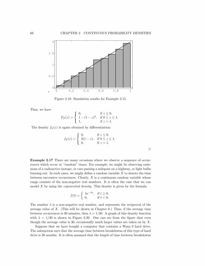
66 CHAPTER 2. CONTINUOUS PROBABILITY DENSITIES
0 0.2 0.4 0.6 0.8 10
0.5
1
1.5
2
Figure 2.18: Simulation results for Example 2.15.
Thus, we have
FZ(z) =
0, if z ≤ 0,1− (1− z)2, if 0 ≤ z ≤ 1,1, if z > 1.
The density fZ(z) is again obtained by differentiation:
fZ(z) =
0, if z ≤ 0,2(1− z), if 0 ≤ z ≤ 1,0, if z > 1.
2
Example 2.17 There are many occasions where we observe a sequence of occur-rences which occur at “random” times. For example, we might be observing emis-sions of a radioactive isotope, or cars passing a milepost on a highway, or light bulbsburning out. In such cases, we might define a random variable X to denote the timebetween successive occurrences. Clearly, X is a continuous random variable whoserange consists of the non-negative real numbers. It is often the case that we canmodel X by using the exponential density . This density is given by the formula
f(t) =λe−λt, if t ≥ 0,0, if t < 0.
The number λ is a non-negative real number, and represents the reciprocal of theaverage value of X. (This will be shown in Chapter 6.) Thus, if the average timebetween occurrences is 30 minutes, then λ = 1/30. A graph of this density functionwith λ = 1/30 is shown in Figure 2.20. One can see from the figure that eventhough the average value is 30, occasionally much larger values are taken on by X.
Suppose that we have bought a computer that contains a Warp 9 hard drive.The salesperson says that the average time between breakdowns of this type of harddrive is 30 months. It is often assumed that the length of time between breakdowns

2.2. CONTINUOUS DENSITY FUNCTIONS 67
E
1 - z
1 - z
1 - z
1 - z
E
Figure 2.19: Calculation of FZ .
20 40 60 80 100 120
0.005
0.01
0.015
0.02
0.025
0.03
f (t) = (1/30) e - (1/30) t
Figure 2.20: Exponential density with λ = 1/30.

68 CHAPTER 2. CONTINUOUS PROBABILITY DENSITIES
0 20 40 60 80 100
0
0.005
0.01
0.015
0.02
0.025
0.03
Figure 2.21: Residual lifespan of a hard drive.
is distributed according to the exponential density. We will assume that this modelapplies here, with λ = 1/30.
Now suppose that we have been operating our computer for 15 months. Weassume that the original hard drive is still running. We ask how long we shouldexpect the hard drive to continue to run. One could reasonably expect that thehard drive will run, on the average, another 15 months. (One might also guessthat it will run more than 15 months, since the fact that it has already run for 15months implies that we don’t have a lemon.) The time which we have to wait isa new random variable, which we will call Y . Obviously, Y = X − 15. We canwrite a computer program to produce a sequence of simulated Y -values. To do this,we first produce a sequence of X’s, and discard those values which are less thanor equal to 15 (these values correspond to the cases where the hard drive has quitrunning before 15 months). To simulate a value of X, we compute the value of theexpression
(− 1λ
)log(rnd) ,
where rnd represents a random real number between 0 and 1. (That this expressionhas the exponential density will be shown in Chapter 4.3.) Figure 2.21 shows anarea bar graph of 10,000 simulated Y -values.
The average value of Y in this simulation is 29.74, which is closer to the originalaverage life span of 30 months than to the value of 15 months which was guessedabove. Also, the distribution of Y is seen to be close to the distribution of X.It is in fact the case that X and Y have the same distribution. This property iscalled the memoryless property , because the amount of time that we have to waitfor an occurrence does not depend on how long we have already waited. The onlycontinuous density function with this property is the exponential density. 2

2.2. CONTINUOUS DENSITY FUNCTIONS 69
Assignment of Probabilities
A fundamental question in practice is: How shall we choose the probability densityfunction in describing any given experiment? The answer depends to a great extenton the amount and kind of information available to us about the experiment. Insome cases, we can see that the outcomes are equally likely. In some cases, we cansee that the experiment resembles another already described by a known density.In some cases, we can run the experiment a large number of times and make areasonable guess at the density on the basis of the observed distribution of outcomes,as we did in Chapter 1. In general, the problem of choosing the right density functionfor a given experiment is a central problem for the experimenter and is not alwayseasy to solve (see Example 2.6). We shall not examine this question in detail herebut instead shall assume that the right density is already known for each of theexperiments under study.
The introduction of suitable coordinates to describe a continuous sample space,and a suitable density to describe its probabilities, is not always so obvious, as ourfinal example shows.
Infinite Tree
Example 2.18 Consider an experiment in which a fair coin is tossed repeatedly,without stopping. We have seen in Example 1.6 that, for a coin tossed n times, thenatural sample space is a binary tree with n stages. On this evidence we expectthat for a coin tossed repeatedly, the natural sample space is a binary tree with aninfinite number of stages, as indicated in Figure 2.22.
It is surprising to learn that, although the n-stage tree is obviously a finite samplespace, the unlimited tree can be described as a continuous sample space. To see howthis comes about, let us agree that a typical outcome of the unlimited coin tossingexperiment can be described by a sequence of the form ω = H H T H T T H . . ..If we write 1 for H and 0 for T, then ω = 1 1 0 1 0 0 1 . . .. In this way, eachoutcome is described by a sequence of 0’s and 1’s.
Now suppose we think of this sequence of 0’s and 1’s as the binary expansionof some real number x = .1101001 · · · lying between 0 and 1. (A binary expansionis like a decimal expansion but based on 2 instead of 10.) Then each outcome isdescribed by a value of x, and in this way x becomes a coordinate for the samplespace, taking on all real values between 0 and 1. (We note that it is possible fortwo different sequences to correspond to the same real number; for example, thesequences T H H H H H . . . and H T T T T T . . . both correspond to the realnumber 1/2. We will not concern ourselves with this apparent problem here.)
What probabilities should be assigned to the events of this sample space? Con-sider, for example, the event E consisting of all outcomes for which the first tosscomes up heads and the second tails. Every such outcome has the form .10∗∗∗∗ · · ·,where ∗ can be either 0 or 1. Now if x is our real-valued coordinate, then the valueof x for every such outcome must lie between 1/2 = .10000 · · · and 3/4 = .11000 · · ·,and moreover, every value of x between 1/2 and 3/4 has a binary expansion of the

70 CHAPTER 2. CONTINUOUS PROBABILITY DENSITIES
0
1
1
1
1
1
1
1
1
1
0
0
0
0
0
0
0
0(start)
1
1
1
1
1
1
1
0
0
0
0 0
0
0
Figure 2.22: Tree for infinite number of tosses of a coin.
form .10 ∗ ∗ ∗ ∗ · · ·. This means that ω ∈ E if and only if 1/2 ≤ x < 3/4, and in thisway we see that we can describe E by the interval [1/2, 3/4). More generally, everyevent consisting of outcomes for which the results of the first n tosses are prescribedis described by a binary interval of the form [k/2n, (k + 1)/2n).
We have already seen in Section 1.2 that in the experiment involving n tosses,the probability of any one outcome must be exactly 1/2n. It follows that in theunlimited toss experiment, the probability of any event consisting of outcomes forwhich the results of the first n tosses are prescribed must also be 1/2n. But 1/2n isexactly the length of the interval of x-values describing E! Thus we see that, just aswith the spinner experiment, the probability of an event E is determined by whatfraction of the unit interval lies in E.
Consider again the statement: The probability is 1/2 that a fair coin will turn upheads when tossed. We have suggested that one interpretation of this statement isthat if we toss the coin indefinitely the proportion of heads will approach 1/2. Thatis, in our correspondence with binary sequences we expect to get a binary sequencewith the proportion of 1’s tending to 1/2. The event E of binary sequences for whichthis is true is a proper subset of the set of all possible binary sequences. It doesnot contain, for example, the sequence 011011011 . . . (i.e., (011) repeated again andagain). The event E is actually a very complicated subset of the binary sequences,but its probability can be determined as a limit of probabilities for events with afinite number of outcomes whose probabilities are given by finite tree measures.When the probability of E is computed in this way, its value is found to be 1.This remarkable result is known as the Strong Law of Large Numbers (or Law ofAverages) and is one justification for our frequency concept of probability. We shallprove a weak form of this theorem in Chapter 8. 2

2.2. CONTINUOUS DENSITY FUNCTIONS 71
Exercises
1 Suppose you choose at random a real number X from the interval [2, 10].
(a) Find the density function f(x) and the probability of an event E for thisexperiment, where E is a subinterval [a, b] of [2, 10].
(b) From (a), find the probability that X > 5, that 5 < X < 7, and thatX2 − 12X + 35 > 0.
2 Suppose you choose a real number X from the interval [2, 10] with a densityfunction of the form
f(x) = Cx ,
where C is a constant.
(a) Find C.
(b) Find P (E), where E = [a, b] is a subinterval of [2, 10].
(c) Find P (X > 5), P (X < 7), and P (X2 − 12X + 35 > 0).
3 Same as Exercise 2, but suppose
f(x) =C
x.
4 Suppose you throw a dart at a circular target of radius 10 inches. Assumingthat you hit the target and that the coordinates of the outcomes are chosenat random, find the probability that the dart falls
(a) within 2 inches of the center.
(b) within 2 inches of the rim.
(c) within the first quadrant of the target.
(d) within the first quadrant and within 2 inches of the rim.
5 Suppose you are watching a radioactive source that emits particles at a ratedescribed by the exponential density
f(t) = λe−λt ,
where λ = 1, so that the probability P (0, T ) that a particle will appear inthe next T seconds is P ([0, T ]) =
∫ T0λe−λt dt. Find the probability that a
particle (not necessarily the first) will appear
(a) within the next second.
(b) within the next 3 seconds.
(c) between 3 and 4 seconds from now.
(d) after 4 seconds from now.

72 CHAPTER 2. CONTINUOUS PROBABILITY DENSITIES
6 Assume that a new light bulb will burn out after t hours, where t is chosenfrom [0,∞) with an exponential density
f(t) = λe−λt .
In this context, λ is often called the failure rate of the bulb.
(a) Assume that λ = 0.01, and find the probability that the bulb will notburn out before T hours. This probability is often called the reliabilityof the bulb.
(b) For what T is the reliability of the bulb = 1/2?
7 Choose a number B at random from the interval [0, 1] with uniform density.Find the probability that
(a) 1/3 < B < 2/3.
(b) |B − 1/2| ≤ 1/4.
(c) B < 1/4 or 1−B < 1/4.
(d) 3B2 < B.
8 Choose independently two numbers B and C at random from the interval [0, 1]with uniform density. Note that the point (B,C) is then chosen at random inthe unit square. Find the probability that
(a) B + C < 1/2.
(b) BC < 1/2.
(c) |B − C| < 1/2.
(d) maxB,C < 1/2.
(e) minB,C < 1/2.
(f) B < 1/2 and 1− C < 1/2.
(g) conditions (c) and (f) both hold.
(h) B2 + C2 ≤ 1/2.
(i) (B − 1/2)2 + (C − 1/2)2 < 1/4.
9 Suppose that we have a sequence of occurrences. We assume that the timeX between occurrences is exponentially distributed with λ = 1/10, so on theaverage, there is one occurrence every 10 minutes (see Example 2.17). Youcome upon this system at time 100, and wait until the next occurrence. Makea conjecture concerning how long, on the average, you will have to wait. Writea program to see if your conjecture is right.
10 As in Exercise 9, assume that we have a sequence of occurrences, but nowassume that the time X between occurrences is uniformly distributed between5 and 15. As before, you come upon this system at time 100, and wait untilthe next occurrence. Make a conjecture concerning how long, on the average,you will have to wait. Write a program to see if your conjecture is right.

2.2. CONTINUOUS DENSITY FUNCTIONS 73
11 For examples such as those in Exercises 9 and 10, it might seem that at leastyou should not have to wait on average more than 10 minutes if the averagetime between occurrences is 10 minutes. Alas, even this is not true. To seewhy, consider the following assumption about the times between occurrences.Assume that the time between occurrences is 3 minutes with probability .9and 73 minutes with probability .1. Show by simulation that the average timebetween occurrences is 10 minutes, but that if you come upon this system attime 100, your average waiting time is more than 10 minutes.
12 Take a stick of unit length and break it into three pieces, choosing the breakpoints at random. (The break points are assumed to be chosen simultane-ously.) What is the probability that the three pieces can be used to form atriangle? Hint : The sum of the lengths of any two pieces must exceed thelength of the third, so each piece must have length < 1/2. Now use Exer-cise 8(g).
13 Take a stick of unit length and break it into two pieces, choosing the breakpoint at random. Now break the longer of the two pieces at a random point.What is the probability that the three pieces can be used to form a triangle?
14 Choose independently two numbers B and C at random from the interval[−1, 1] with uniform distribution, and consider the quadratic equation
x2 +Bx+ C = 0 .
Find the probability that the roots of this equation
(a) are both real.
(b) are both positive.
Hints: (a) requires 0 ≤ B2 − 4C, (b) requires 0 ≤ B2 − 4C, B ≤ 0, 0 ≤ C.
15 At the Tunbridge World’s Fair, a coin toss game works as follows. Quartersare tossed onto a checkerboard. The management keeps all the quarters, butfor each quarter landing entirely within one square of the checkerboard themanagement pays a dollar. Assume that the edge of each square is twice thediameter of a quarter, and that the outcomes are described by coordinateschosen at random. Is this a fair game?
16 Three points are chosen at random on a circle of unit circumference. What isthe probability that the triangle defined by these points as vertices has threeacute angles? Hint : One of the angles is obtuse if and only if all three pointslie in the same semicircle. Take the circumference as the interval [0, 1]. Takeone point at 0 and the others at B and C.
17 Write a program to choose a random number X in the interval [2, 10] 1000times and record what fraction of the outcomes satisfy X > 5, what fractionsatisfy 5 < X < 7, and what fraction satisfy x2− 12x+ 35 > 0. How do theseresults compare with Exercise 1?

74 CHAPTER 2. CONTINUOUS PROBABILITY DENSITIES
18 Write a program to choose a point (X,Y ) at random in a square of side 20inches, doing this 10,000 times, and recording what fraction of the outcomesfall within 19 inches of the center; of these, what fraction fall between 8 and 10inches of the center; and, of these, what fraction fall within the first quadrantof the square. How do these results compare with those of Exercise 4?
19 Write a program to simulate the problem describe in Exercise 7 (see Exer-cise 17). How do the simulation results compare with the results of Exercise 7?
20 Write a program to simulate the problem described in Exercise 12.
21 Write a program to simulate the problem described in Exercise 16.
22 Write a program to carry out the following experiment. A coin is tossed 100times and the number of heads that turn up is recorded. This experimentis then repeated 1000 times. Have your program plot a bar graph for theproportion of the 1000 experiments in which the number of heads is n, foreach n in the interval [35, 65]. Does the bar graph look as though it can be fitwith a normal curve?
23 Write a program that picks a random number between 0 and 1 and computesthe negative of its logarithm. Repeat this process a large number of times andplot a bar graph to give the number of times that the outcome falls in eachinterval of length 0.1 in [0, 10]. On this bar graph plot a graph of the densityf(x) = e−x. How well does this density fit your graph?

Chapter 3
Combinatorics
3.1 Permutations
Many problems in probability theory require that we count the number of waysthat a particular event can occur. For this, we study the topics of permutations andcombinations. We consider permutations in this section and combinations in thenext section.
Before discussing permutations, it is useful to introduce a general counting tech-nique that will enable us to solve a variety of counting problems, including theproblem of counting the number of possible permutations of n objects.
Counting Problems
Consider an experiment that takes place in several stages and is such that thenumber of outcomes m at the nth stage is independent of the outcomes of theprevious stages. The number m may be different for different stages. We want tocount the number of ways that the entire experiment can be carried out.
Example 3.1 You are eating at Emile’s restaurant and the waiter informs youthat you have (a) two choices for appetizers: soup or juice; (b) three for the maincourse: a meat, fish, or vegetable dish; and (c) two for dessert: ice cream or cake.How many possible choices do you have for your complete meal? We illustrate thepossible meals by a tree diagram shown in Figure 3.1. Your menu is decided in threestages—at each stage the number of possible choices does not depend on what ischosen in the previous stages: two choices at the first stage, three at the second,and two at the third. From the tree diagram we see that the total number of choicesis the product of the number of choices at each stage. In this examples we have2 · 3 · 2 = 12 possible menus. Our menu example is an example of the followinggeneral counting technique. 2
75
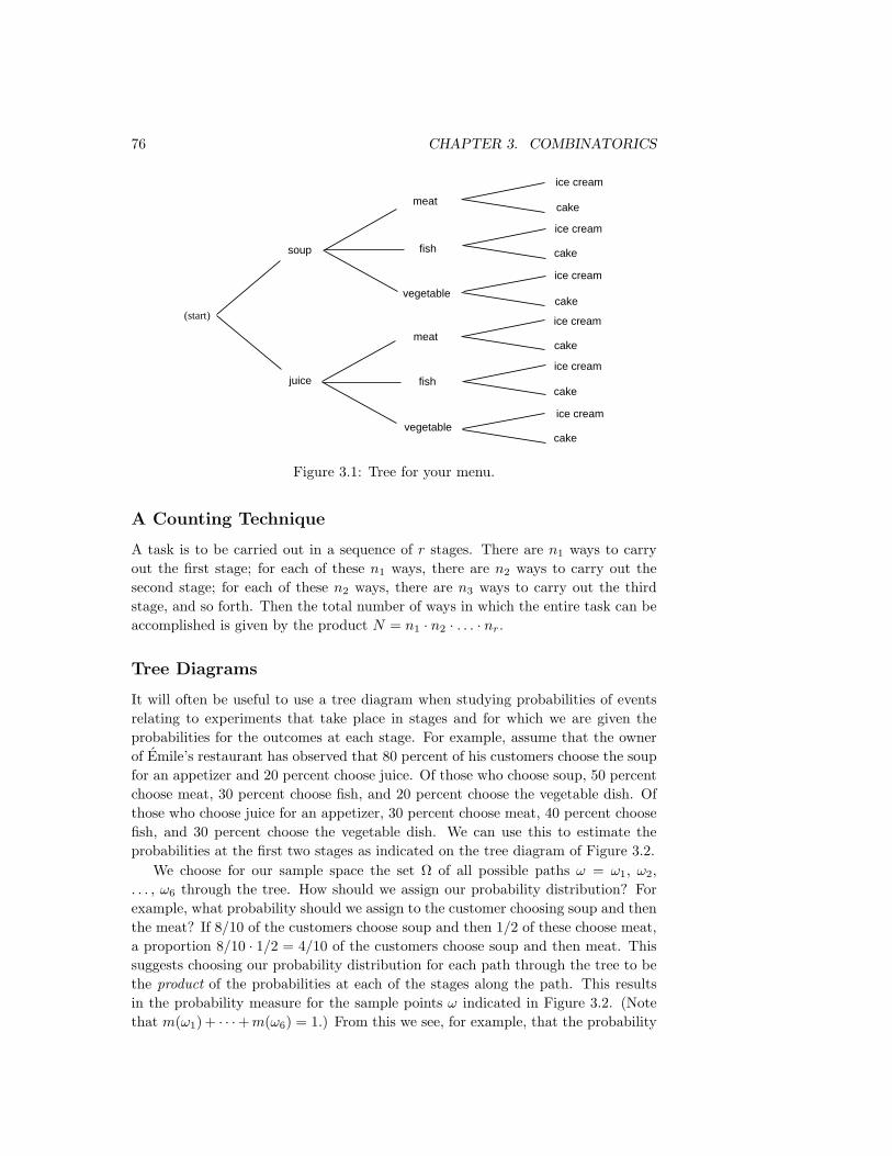
76 CHAPTER 3. COMBINATORICS
ice cream
cake
ice cream
cake
ice cream
cake
ice cream
cake
ice cream
cake
ice cream
cake
(start)
soup
meat
fish
vegetable
juice
meat
fish
vegetable
Figure 3.1: Tree for your menu.
A Counting Technique
A task is to be carried out in a sequence of r stages. There are n1 ways to carryout the first stage; for each of these n1 ways, there are n2 ways to carry out thesecond stage; for each of these n2 ways, there are n3 ways to carry out the thirdstage, and so forth. Then the total number of ways in which the entire task can beaccomplished is given by the product N = n1 · n2 · . . . · nr.
Tree Diagrams
It will often be useful to use a tree diagram when studying probabilities of eventsrelating to experiments that take place in stages and for which we are given theprobabilities for the outcomes at each stage. For example, assume that the ownerof Emile’s restaurant has observed that 80 percent of his customers choose the soupfor an appetizer and 20 percent choose juice. Of those who choose soup, 50 percentchoose meat, 30 percent choose fish, and 20 percent choose the vegetable dish. Ofthose who choose juice for an appetizer, 30 percent choose meat, 40 percent choosefish, and 30 percent choose the vegetable dish. We can use this to estimate theprobabilities at the first two stages as indicated on the tree diagram of Figure 3.2.
We choose for our sample space the set Ω of all possible paths ω = ω1, ω2,. . . , ω6 through the tree. How should we assign our probability distribution? Forexample, what probability should we assign to the customer choosing soup and thenthe meat? If 8/10 of the customers choose soup and then 1/2 of these choose meat,a proportion 8/10 · 1/2 = 4/10 of the customers choose soup and then meat. Thissuggests choosing our probability distribution for each path through the tree to bethe product of the probabilities at each of the stages along the path. This resultsin the probability measure for the sample points ω indicated in Figure 3.2. (Notethat m(ω1) + · · ·+m(ω6) = 1.) From this we see, for example, that the probability

3.1. PERMUTATIONS 77
(start)
soup
meat
fish
vegetable
juice
.8
.2
.2
.3
.3
.4
.5
.3
meat
fish
vegetable
ω (ω)
ω
ω
ω
ω
ω
ω
.4
.24
.16
.06
.08
.06
m
1
2
3
4
5
6
Figure 3.2: Two-stage probability assignment.
that a customer chooses meat is m(ω1) +m(ω4) = .46.We shall say more about these tree measures when we discuss the concept of
conditional probability in Chapter 4. We return now to more counting problems.
Example 3.2 We can show that there are at least two people in Columbus, Ohio,who have the same three initials. Assuming that each person has three initials,there are 26 possibilities for a person’s first initial, 26 for the second, and 26 for thethird. Therefore, there are 263 = 17,576 possible sets of initials. This number issmaller than the number of people living in Columbus, Ohio; hence, there must beat least two people with the same three initials. 2
We consider next the celebrated birthday problem—often used to show thatnaive intuition cannot always be trusted in probability.
Birthday Problem
Example 3.3 How many people do we need to have in a room to make it a favorablebet (probability of success greater than 1/2) that two people in the room will havethe same birthday?
Since there are 365 possible birthdays, it is tempting to guess that we wouldneed about 1/2 this number, or 183. You would surely win this bet. In fact, thenumber required for a favorable bet is only 23. To show this, we find the probabilitypr that, in a room with r people, there is no duplication of birthdays; we will havea favorable bet if this probability is less than one half.

78 CHAPTER 3. COMBINATORICS
Number of people Probability that all birthdays are different
20 .588561621 .556311722 .524304723 .492702824 .461655725 .4313003
Table 3.1: Birthday problem.
Assume that there are 365 possible birthdays for each person (we ignore leapyears). Order the people from 1 to r. For a sample point ω, we choose a possiblesequence of length r of birthdays each chosen as one of the 365 possible dates.There are 365 possibilities for the first element of the sequence, and for each ofthese choices there are 365 for the second, and so forth, making 365r possiblesequences of birthdays. We must find the number of these sequences that have noduplication of birthdays. For such a sequence, we can choose any of the 365 daysfor the first element, then any of the remaining 364 for the second, 363 for the third,and so forth, until we make r choices. For the rth choice, there will be 365− r + 1possibilities. Hence, the total number of sequences with no duplications is
365 · 364 · 363 · . . . · (365− r + 1) .
Thus, assuming that each sequence is equally likely,
pr =365 · 364 · . . . · (365− r + 1)
365r.
We denote the product(n)(n− 1) · · · (n− r + 1)
by (n)r (read “n down r,” or “n lower r”). Thus,
pr =(365)r(365)r
.
The program Birthday carries out this computation and prints the probabilitiesfor r = 20 to 25. Running this program, we get the results shown in Table 3.1. Aswe asserted above, the probability for no duplication changes from greater than onehalf to less than one half as we move from 22 to 23 people. To see how unlikely it isthat we would lose our bet for larger numbers of people, we have run the programagain, printing out values from r = 10 to r = 100 in steps of 10. We see that ina room of 40 people the odds already heavily favor a duplication, and in a roomof 100 the odds are overwhelmingly in favor of a duplication. We have assumedthat birthdays are equally likely to fall on any particular day. Statistical evidencesuggests that this is not true. However, it is intuitively clear (but not easy to prove)that this makes it even more likely to have a duplication with a group of 23 people.(See Exercise 19 to find out what happens on planets with more or fewer than 365days per year.) 2

3.1. PERMUTATIONS 79
Number of people Probability that all birthdays are different
10 .883051820 .588561630 .293683840 .108768250 .029626460 .005877370 .000840480 .000085790 .0000062100 .0000003
Table 3.2: Birthday problem.
We now turn to the topic of permutations.
Permutations
Definition 3.1 Let A be any finite set. A permutation of A is a one-to-one mappingof A onto itself. 2
To specify a particular permutation we list the elements of A and, under them,show where each element is sent by the one-to-one mapping. For example, if A =a, b, c a possible permutation σ would be
σ =(a b c
b c a
).
By the permutation σ, a is sent to b, b is sent to c, and c is sent to a. Thecondition that the mapping be one-to-one means that no two elements of A aresent, by the mapping, into the same element of A.
We can put the elements of our set in some order and rename them 1, 2, . . . , n.Then, a typical permutation of the set A = a1, a2, a3, a4 can be written in theform
σ =(
1 2 3 42 1 4 3
),
indicating that a1 went to a2, a2 to a1, a3 to a4, and a4 to a3.If we always choose the top row to be 1 2 3 4 then, to prescribe the permutation,
we need only give the bottom row, with the understanding that this tells us where 1goes, 2 goes, and so forth, under the mapping. When this is done, the permutationis often called a rearrangement of the n objects 1, 2, 3, . . . , n. For example, allpossible permutations, or rearrangements, of the numbers A = 1, 2, 3 are:
123, 132, 213, 231, 312, 321 .
It is an easy matter to count the number of possible permutations of n objects.By our general counting principle, there are n ways to assign the first element, for

80 CHAPTER 3. COMBINATORICS
n n!
0 11 12 23 64 245 1206 7207 50408 403209 362880
10 3628800
Table 3.3: Values of the factorial function.
each of these we have n − 1 ways to assign the second object, n − 2 for the third,and so forth. This proves the following theorem.
Theorem 3.1 The total number of permutations of a set A of n elements is givenby n · (n − 1) · (n− 2) · . . . · 1. 2
It is sometimes helpful to consider orderings of subsets of a given set. Thisprompts the following definition.
Definition 3.2 Let A be an n-element set, and let k be an integer between 0 andn. Then a k-permutation of A is an ordered listing of a subset of A of size k. 2
Using the same techniques as in the last theorem, the following result is easilyproved.
Theorem 3.2 The total number of k-permutations of a set A of n elements is givenby n · (n− 1) · (n− 2) · . . . · (n− k + 1). 2
Factorials
The number given in Theorem 3.1 is called n factorial, and is denoted by n!. Theexpression 0! is defined to be 1 to make certain formulas come out simpler. Thefirst few values of this function are shown in Table 3.3. The reader will note thatthis function grows very rapidly.
The expression n! will enter into many of our calculations, and we shall need tohave some estimate of its magnitude when n is large. It is clearly not practical tomake exact calculations in this case. We shall instead use a result called Stirling’sformula. Before stating this formula we need a definition.

3.1. PERMUTATIONS 81
n n! Approximation Ratio
1 1 .922 1.0842 2 1.919 1.0423 6 5.836 1.0284 24 23.506 1.0215 120 118.019 1.0166 720 710.078 1.0137 5040 4980.396 1.0118 40320 39902.395 1.0109 362880 359536.873 1.009
10 3628800 3598696.619 1.008
Table 3.4: Stirling approximations to the factorial function.
Definition 3.3 Let an and bn be two sequences of numbers. We say that an isasymptotically equal to bn, and write an ∼ bn, if
limn→∞
anbn
= 1 .
2
Example 3.4 If an = n+√n and bn = n then, since an/bn = 1 + 1/
√n and this
ratio tends to 1 as n tends to infinity, we have an ∼ bn. 2
Theorem 3.3 (Stirling’s Formula) The sequence n! is asymptotically equal to
nne−n√
2πn .
2
The proof of Stirling’s formula may be found in most analysis texts. Let usverify this approximation by using the computer. The program StirlingApprox-imations prints n!, the Stirling approximation, and, finally, the ratio of these twonumbers. Sample output of this program is shown in Table 3.4. Note that, whilethe ratio of the numbers is getting closer to 1, the difference between the exactvalue and the approximation is increasing, and indeed, this difference will tend toinfinity as n tends to infinity, even though the ratio tends to 1. (This was also truein our Example 3.4 where n+
√n ∼ n, but the difference is
√n.)
Generating Random Permutations
We now consider the question of generating a random permutation of the integersbetween 1 and n. Consider the following experiment. We start with a deck of ncards, labelled 1 through n. We choose a random card out of the deck, note its label,and put the card aside. We repeat this process until all n cards have been chosen.It is clear that each permutation of the integers from 1 to n can occur as a sequence

82 CHAPTER 3. COMBINATORICS
Number of fixed points Fraction of permutationsn = 10 n = 20 n = 30
0 .362 .370 .3581 .368 .396 .3582 .202 .164 .1923 .052 .060 .0704 .012 .008 .0205 .004 .002 .002
Average number of fixed points .996 .948 1.042
Table 3.5: Fixed point distributions.
of labels in this experiment, and that each sequence of labels is equally likely tooccur. In our implementations of the computer algorithms, the above procedure iscalled RandomPermutation.
Fixed Points
There are many interesting problems that relate to properties of a permutationchosen at random from the set of all permutations of a given finite set. For example,since a permutation is a one-to-one mapping of the set onto itself, it is interesting toask how many points are mapped onto themselves. We call such points fixed pointsof the mapping.
Let pk(n) be the probability that a random permutation of the set 1, 2, . . . , nhas exactly k fixed points. We will attempt to learn something about these prob-abilities using simulation. The program FixedPoints uses the procedure Ran-domPermutation to generate random permutations and count fixed points. Theprogram prints the proportion of times that there are k fixed points as well as theaverage number of fixed points. The results of this program for 500 simulations forthe cases n = 10, 20, and 30 are shown in Table 3.5. Notice the rather surprisingfact that our estimates for the probabilities do not seem to depend very heavily onthe number of elements in the permutation. For example, the probability that thereare no fixed points, when n = 10, 20, or 30 is estimated to be between .35 and .37.We shall see later (see Example 3.12) that for n ≥ 10 the exact probabilities pn(0)are, to six decimal place accuracy, equal to 1/e ≈ .367879. Thus, for all practi-cal purposes, after n = 10 the probability that a random permutation of the set1, 2, . . . , n has no fixed points does not depend upon n. These simulations alsosuggest that the average number of fixed points is close to 1. It can be shown (seeExample 6.8) that the average is exactly equal to 1 for all n.
More picturesque versions of the fixed-point problem are: You have arrangedthe books on your book shelf in alphabetical order by author and they get returnedto your shelf at random; what is the probability that exactly k of the books end upin their correct position? (The library problem.) In a restaurant n hats are checkedand they are hopelessly scrambled; what is the probability that no one gets his ownhat back? (The hat check problem.) In the Historical Remarks at the end of thissection, we give one method for solving the hat check problem exactly. Another
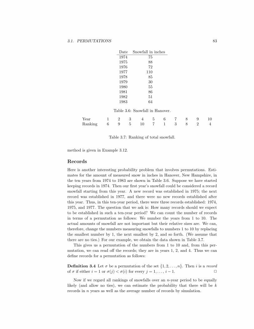
3.1. PERMUTATIONS 83
Date Snowfall in inches1974 751975 881976 721977 1101978 851979 301980 551981 861982 511983 64
Table 3.6: Snowfall in Hanover.
Year 1 2 3 4 5 6 7 8 9 10Ranking 6 9 5 10 7 1 3 8 2 4
Table 3.7: Ranking of total snowfall.
method is given in Example 3.12.
Records
Here is another interesting probability problem that involves permutations. Esti-mates for the amount of measured snow in inches in Hanover, New Hampshire, inthe ten years from 1974 to 1983 are shown in Table 3.6. Suppose we have startedkeeping records in 1974. Then our first year’s snowfall could be considered a recordsnowfall starting from this year. A new record was established in 1975; the nextrecord was established in 1977, and there were no new records established afterthis year. Thus, in this ten-year period, there were three records established: 1974,1975, and 1977. The question that we ask is: How many records should we expectto be established in such a ten-year period? We can count the number of recordsin terms of a permutation as follows: We number the years from 1 to 10. Theactual amounts of snowfall are not important but their relative sizes are. We can,therefore, change the numbers measuring snowfalls to numbers 1 to 10 by replacingthe smallest number by 1, the next smallest by 2, and so forth. (We assume thatthere are no ties.) For our example, we obtain the data shown in Table 3.7.
This gives us a permutation of the numbers from 1 to 10 and, from this per-mutation, we can read off the records; they are in years 1, 2, and 4. Thus we candefine records for a permutation as follows:
Definition 3.4 Let σ be a permutation of the set 1, 2, . . . , n. Then i is a recordof σ if either i = 1 or σ(j) < σ(i) for every j = 1, . . . , i− 1. 2
Now if we regard all rankings of snowfalls over an n-year period to be equallylikely (and allow no ties), we can estimate the probability that there will be k
records in n years as well as the average number of records by simulation.

84 CHAPTER 3. COMBINATORICS
We have written a program Records that counts the number of records in ran-domly chosen permutations. We have run this program for the cases n = 10, 20, 30.For n = 10 the average number of records is 2.968, for 20 it is 3.656, and for 30it is 3.960. We see now that the averages increase, but very slowly. We shall seelater (see Example 6.11) that the average number is approximately logn. Sincelog 10 = 2.3, log 20 = 3, and log 30 = 3.4, this is consistent with the results of oursimulations.
As remarked earlier, we shall be able to obtain formulas for exact results ofcertain problems of the above type. However, only minor changes in the problemmake this impossible. The power of simulation is that minor changes in a problemdo not make the simulation much more difficult. (See Exercise 20 for an interestingvariation of the hat check problem.)
List of Permutations
Another method to solve problems that is not sensitive to small changes in theproblem is to have the computer simply list all possible permutations and count thefraction that have the desired property. The program AllPermutations producesa list of all of the permutations of n. When we try running this program, we runinto a limitation on the use of the computer. The number of permutations of nincreases so rapidly that even to list all permutations of 20 objects is impractical.
Historical Remarks
Our basic counting principle stated that if you can do one thing in r ways and foreach of these another thing in s ways, then you can do the pair in rs ways. Thisis such a self-evident result that you might expect that it occurred very early inmathematics. N. L. Biggs suggests that we might trace an example of this principleas follows: First, he relates a popular nursery rhyme dating back to at least 1730:
As I was going to St. Ives,I met a man with seven wives,Each wife had seven sacks,Each sack had seven cats,Each cat had seven kits.Kits, cats, sacks and wives,How many were going to St. Ives?
(You need our principle only if you are not clever enough to realize that you aresupposed to answer one, since only the narrator is going to St. Ives; the others aregoing in the other direction!)
He also gives a problem appearing on one of the oldest surviving mathematicalmanuscripts of about 1650 B.C., roughly translated as:

3.1. PERMUTATIONS 85
Houses 7Cats 49Mice 343Wheat 2401Hekat 16807
19607
The following interpretation has been suggested: there are seven houses, eachwith seven cats; each cat kills seven mice; each mouse would have eaten seven headsof wheat, each of which would have produced seven hekat measures of grain. Withthis interpretation, the table answers the question of how many hekat measureswere saved by the cats’ actions. It is not clear why the writer of the table wantedto add the numbers together.1
One of the earliest uses of factorials occurred in Euclid’s proof that there areinfinitely many prime numbers. Euclid argued that there must be a prime numberbetween n and n! + 1 as follows: n! and n! + 1 cannot have common factors. Eithern! + 1 is prime or it has a proper factor. In the latter case, this factor cannot dividen! and hence must be between n and n! + 1. If this factor is not prime, then ithas a factor that, by the same argument, must be bigger than n. In this way, weeventually reach a prime bigger than n, and this holds for all n.
The “n!” rule for the number of permutations seems to have occurred first inIndia. Examples have been found as early as 300 B.C., and by the eleventh centurythe general formula seems to have been well known in India and then in the Arabcountries.
The hat check problem is found in an early probability book written by de Mont-mort and first printed in 1708.2 It appears in the form of a game called Treize. Ina simplified version of this game considered by de Montmort one turns over cardsnumbered 1 to 13, calling out 1, 2, . . . , 13 as the cards are examined. De Montmortasked for the probability that no card that is turned up agrees with the numbercalled out.
This probability is the same as the probability that a random permutation of13 elements has no fixed point. De Montmort solved this problem by the use of arecursion relation as follows: let wn be the number of permutations of n elementswith no fixed point (such permutations are called derangements). Then w1 = 0 andw2 = 1.
Now assume that n ≥ 3 and choose a derangement of the integers between 1 andn. Let k be the integer in the first position in this derangement. By the definition ofderangement, we have k 6= 1. There are two possibilities of interest concerning theposition of 1 in the derangement: either 1 is in the kth position or it is elsewhere. Inthe first case, the n− 2 remaining integers can be positioned in wn−2 ways withoutresulting in any fixed points. In the second case, we consider the set of integers1, 2, . . . , k − 1, k + 1, . . . , n. The numbers in this set must occupy the positions2, 3, . . . , n so that none of the numbers other than 1 in this set are fixed, and
1N. L. Biggs, “The Roots of Combinatorics,” Historia Mathematica, vol. 6 (1979), pp. 109–136.2P. R. de Montmort, Essay d’Analyse sur des Jeux de Hazard, 2d ed. (Paris: Quillau, 1713).

86 CHAPTER 3. COMBINATORICS
also so that 1 is not in position k. The number of ways of achieving this kind ofarrangement is just wn−1. Since there are n− 1 possible values of k, we see that
wn = (n− 1)wn−1 + (n− 1)wn−2
for n ≥ 3. One might conjecture from this last equation that the sequence wngrows like the sequence n!.
In fact, it is easy to prove by induction that
wn = nwn−1 + (−1)n .
Then pi = wi/i! satisfies
pi − pi−1 =(−1)i
i!.
If we sum from i = 2 to n, and use the fact that p1 = 0, we obtain
pn =12!− 1
3!+ · · ·+ (−1)n
n!.
This agrees with the first n+ 1 terms of the expansion for ex for x = −1 and hencefor large n is approximately e−1 ≈ .368. David remarks that this was possiblythe first use of the exponential function in probability.3 We shall see another wayto derive de Montmort’s result in the next section, using a method known as theInclusion-Exclusion method.
Recently, a related problem appeared in a column of Marilyn vos Savant.4
Charles Price wrote to ask about his experience playing a certain form of solitaire,sometimes called “frustration solitaire.” In this particular game, a deck of cardsis shuffled, and then dealt out, one card at a time. As the cards are being dealt,the player counts from 1 to 13, and then starts again at 1. (Thus, each number iscounted four times.) If a number that is being counted coincides with the rank ofthe card that is being turned up, then the player loses the game. Price found thathe rarely won and wondered how often he should win. Vos Savant remarked thatthe expected number of matches is 4 so it should be difficult to win the game.
Finding the chance of winning is a harder problem than the one that de Mont-mort solved because, when one goes through the entire deck, there are differentpatterns for the matches that might occur. For example matches may occur for twocards of the same rank, say two aces, or for two different ranks, say a two and athree.
A discussion of this problem can be found in Riordan.5 In this book, it is shownthat as n→∞, the probability of no matches tends to 1/e4.
The original game of Treize is more difficult to analyze than frustration solitaire.The game of Treize is played as follows. One person is chosen as dealer and theothers are players. Each player, other than the dealer, puts up a stake. The dealershuffles the cards and turns them up one at a time calling out, “Ace, two, three,...,
3F. N. David, Games, Gods and Gambling (London: Griffin, 1962), p. 146.4M. vos Savant, Ask Marilyn, Parade Magazine, Boston Globe, 21 August 1994.5J. Riordan, An Introduction to Combinatorial Analysis, (New York: John Wiley & Sons,
1958).

3.1. PERMUTATIONS 87
king,” just as in frustration solitaire. If the dealer goes through the 13 cards withouta match he pays the players an amount equal to their stake, and the deal passes tosomeone else. If there is a match the dealer collects the players’ stakes; the playersput up new stakes, and the dealer continues through the deck, calling out, “Ace,two, three, ....” If the dealer runs out of cards he reshuffles and continues the countwhere he left off. He continues until there is a run of 13 without a match and thena new dealer is chosen.
The question at this point is how much money can the dealer expect to win fromeach player. De Montmort found that if each player puts up a stake of 1, say, thenthe dealer will win approximately .801 from each player.
Peter Doyle calculated the exact amount that the dealer can expect to win. Theanswer is:
26516072156010218582227607912734182784642120482136091446715371962089931523113435417245543349128705414402992392516076941135000807759178185120138217687665356317385287455585936725463200947740372739557280745938434274787664965076063990538261189388143513547366316017004945507201764278828306601171079536331427343824779227098352817532990359885814136883676558331132447615331072062747416971930180664915269870408438391421790790695497603628528211590140316202120601549126920880824913325553882692055427830810368578188612087582488006809786404381185828348775425609555506628789271230482699760170011623359279330829753364219350507454026892568319388782130144270519791882/33036929133582592220117220713156071114975101149831063364072138969878007996472047088253033875258922365813230156280056211434272906256589744339716571945412290800708628984130608756130281899116735786362375606718498649135353553622197448890223267101158801016285931351979294387223277033396967797970699334758024236769498736616051840314775615603933802570709707119596964126824245501331987974705469351780938375059348885869867236484695053988868628582609905586271001318150621134407056983214740221851567706672080945865893784594327998687063341618129886304963272872548184588793530244980032242558644674104814772093410806135061350385697304897121306393704051559533731591.
This is .803 to 3 decimal places. A description of the algorithm used to find thisanswer can be found on his Web page.6 A discussion of this problem and otherproblems can be found in Doyle et al.7
The birthday problem does not seem to have a very old history. Problems ofthis type were first discussed by von Mises.8 It was made popular in the 1950s byFeller’s book.9
6P. Doyle, “Solution to Montmort’s Probleme du Treize,” http://math.ucsd.edu/ doyle/.7P. Doyle, C. Grinstead, and J. Snell, “Frustration Solitaire,” UMAP Journal , vol. 16, no. 2
(1995), pp. 137-145.8R. von Mises, “Uber Aufteilungs- und Besetzungs-Wahrscheinlichkeiten,” Revue de la Faculte
des Sciences de l’Universite d’Istanbul, N. S. vol. 4 (1938-39), pp. 145-163.9W. Feller, Introduction to Probability Theory and Its Applications, vol. 1, 3rd ed. (New York:

88 CHAPTER 3. COMBINATORICS
Stirling presented his formula
n! ∼√
2πn(ne
)nin his work Methodus Differentialis published in 1730.10 This approximation wasused by de Moivre in establishing his celebrated central limit theorem that wewill study in Chapter 9. De Moivre himself had independently established thisapproximation, but without identifying the constant π. Having established theapproximation
2B√n
for the central term of the binomial distribution, where the constant B was deter-mined by an infinite series, de Moivre writes:
. . . my worthy and learned Friend, Mr. James Stirling, who had appliedhimself after me to that inquiry, found that the Quantity B did denotethe Square-root of the Circumference of a Circle whose Radius is Unity,so that if that Circumference be called c the Ratio of the middle Termto the Sum of all Terms will be expressed by 2/
√nc . . . .11
Exercises
1 Four people are to be arranged in a row to have their picture taken. In howmany ways can this be done?
2 An automobile manufacturer has four colors available for automobile exteri-ors and three for interiors. How many different color combinations can heproduce?
3 In a digital computer, a bit is one of the integers 0,1, and a word is anystring of 32 bits. How many different words are possible?
4 What is the probability that at least 2 of the presidents of the United Stateshave died on the same day of the year? If you bet this has happened, wouldyou win your bet?
5 There are three different routes connecting city A to city B. How many wayscan a round trip be made from A to B and back? How many ways if it isdesired to take a different route on the way back?
6 In arranging people around a circular table, we take into account their seatsrelative to each other, not the actual position of any one person. Show thatn people can be arranged around a circular table in (n− 1)! ways.
John Wiley & Sons, 1968).10J. Stirling, Methodus Differentialis, (London: Bowyer, 1730).11A. de Moivre, The Doctrine of Chances, 3rd ed. (London: Millar, 1756).

3.1. PERMUTATIONS 89
7 Five people get on an elevator that stops at five floors. Assuming that eachhas an equal probability of going to any one floor, find the probability thatthey all get off at different floors.
8 A finite set Ω has n elements. Show that if we count the empty set and Ω assubsets, there are 2n subsets of Ω.
9 A more refined inequality for approximating n! is given by
√2πn
(ne
)ne1/(12n+1) < n! <
√2πn
(ne
)ne1/(12n) .
Write a computer program to illustrate this inequality for n = 1 to 9.
10 A deck of ordinary cards is shuffled and 13 cards are dealt. What is theprobability that the last card dealt is an ace?
11 There are n applicants for the director of computing. The applicants are inter-viewed independently by each member of the three-person search committeeand ranked from 1 to n. A candidate will be hired if he or she is ranked firstby at least two of the three interviewers. Find the probability that a candidatewill be accepted if the members of the committee really have no ability at allto judge the candidates and just rank the candidates randomly. In particular,compare this probability for the case of three candidates and the case of tencandidates.
12 A symphony orchestra has in its repertoire 30 Haydn symphonies, 15 modernworks, and 9 Beethoven symphonies. Its program always consists of a Haydnsymphony followed by a modern work, and then a Beethoven symphony.
(a) How many different programs can it play?
(b) How many different programs are there if the three pieces can be playedin any order?
(c) How many different three-piece programs are there if more than onepiece from the same category can be played and they can be played inany order?
13 A certain state has license plates showing three numbers and three letters.How many different license plates are possible
(a) if the numbers must come before the letters?
(b) if there is no restriction on where the letters and numbers appear?
14 The door on the computer center has a lock which has five buttons numberedfrom 1 to 5. The combination of numbers that opens the lock is a sequenceof five numbers and is reset every week.
(a) How many combinations are possible if every button must be used once?

90 CHAPTER 3. COMBINATORICS
(b) Assume that the lock can also have combinations that require you topush two buttons simultaneously and then the other three one at a time.How many more combinations does this permit?
15 A computing center has 3 processors that receive n jobs, with the jobs assignedto the processors purely at random so that all of the 3n possible assignmentsare equally likely. Find the probability that exactly one processor has no jobs.
16 Prove that at least two people in Atlanta, Georgia, have the same initials,assuming no one has more than four initials.
17 Find a formula for the probability that among a set of n people, at least twohave their birthdays in the same month of the year (assuming the months areequally likely for birthdays).
18 Consider the problem of finding the probability of more than one coincidenceof birthdays in a group of n people. These include, for example, three peoplewith the same birthday, or two pairs of people with the same birthday, orlarger coincidences. Show how you could compute this probability, and writea computer program to carry out this computation. Use your program to findthe smallest number of people for which it would be a favorable bet that therewould be more than one coincidence of birthdays.
*19 Suppose that on planet Zorg a year has n days, and that the lifeforms thereare equally likely to have hatched on any day of the year. We would liketo estimate d, which is the minimum number of lifeforms needed so that theprobability of at least two sharing a birthday exceeds 1/2.
(a) In Example 3.3, it was shown that in a set of d lifeforms, the probabilitythat no two life forms share a birthday is
(n)dnd
,
where (n)d = (n)(n − 1) · · · (n − d + 1). Thus, we would like to set thisequal to 1/2 and solve for d.
(b) Using Stirling’s Formula, show that
(n)dnd∼(
1 +d
n− d
)n−d+1/2
e−d .
(c) Now take the logarithm of the right-hand expression, and use the factthat for small values of x, we have
log(1 + x) ∼ x− x2
2.
(We are implicitly using the fact that d is of smaller order of magnitudethan n. We will also use this fact in part (d).)

3.1. PERMUTATIONS 91
(d) Set the expression found in part (c) equal to − log(2), and solve for d asa function of n, thereby showing that
d ∼√
2(log 2)n .
Hint : If all three summands in the expression found in part (b) are used,one obtains a cubic equation in d. If the smallest of the three terms isthrown away, one obtains a quadratic equation in d.
(e) Use a computer to calculate the exact values of d for various values ofn. Compare these values with the approximate values obtained by usingthe answer to part d).
20 At a mathematical conference, ten participants are randomly seated arounda circular table for meals. Using simulation, estimate the probability that notwo people sit next to each other at both lunch and dinner. Can you make anintelligent conjecture for the case of n participants when n is large?
21 Modify the program AllPermutations to count the number of permutationsof n objects that have exactly j fixed points for j = 0, 1, 2, . . . , n. Runyour program for n = 2 to 6. Make a conjecture for the relation between thenumber that have 0 fixed points and the number that have exactly 1 fixedpoint. A proof of the correct conjecture can be found in Wilf.12
22 Mr. Wimply Dimple, one of London’s most prestigious watch makers, hascome to Sherlock Holmes in a panic, having discovered that someone hasbeen producing and selling crude counterfeits of his best selling watch. The 16counterfeits so far discovered bear stamped numbers, all of which fall between1 and 56, and Dimple is anxious to know the extent of the forger’s work. Allpresent agree that it seems reasonable to assume that the counterfeits thusfar produced bear consecutive numbers from 1 to whatever the total numberis.
“Chin up, Dimple,” opines Dr. Watson. “I shouldn’t worry overly much ifI were you; the Maximum Likelihood Principle, which estimates the totalnumber as precisely that which gives the highest probability for the seriesof numbers found, suggests that we guess 56 itself as the total. Thus, yourforgers are not a big operation, and we shall have them safely behind barsbefore your business suffers significantly.”
“Stuff, nonsense, and bother your fancy principles, Watson,” counters Holmes.“Anyone can see that, of course, there must be quite a few more than 56watches—why the odds of our having discovered precisely the highest num-bered watch made are laughably negligible. A much better guess would betwice 56.”
(a) Show that Watson is correct that the Maximum Likelihood Principlegives 56.
12H. S. Wilf, “A Bijection in the Theory of Derangements,” Mathematics Magazine, vol. 57,no. 1 (1984), pp. 37–40.

92 CHAPTER 3. COMBINATORICS
(b) Write a computer program to compare Holmes’s and Watson’s guessingstrategies as follows: fix a total N and choose 16 integers randomlybetween 1 and N . Let m denote the largest of these. Then Watson’sguess for N is m, while Holmes’s is 2m. See which of these is closer toN . Repeat this experiment (with N still fixed) a hundred or more times,and determine the proportion of times that each comes closer. Whoseseems to be the better strategy?
23 Barbara Smith is interviewing candidates to be her secretary. As she inter-views the candidates, she can determine the relative rank of the candidatesbut not the true rank. Thus, if there are six candidates and their true rank is6, 1, 4, 2, 3, 5, (where 1 is best) then after she had interviewed the first threecandidates she would rank them 3, 1, 2. As she interviews each candidate,she must either accept or reject the candidate. If she does not accept thecandidate after the interview, the candidate is lost to her. She wants to de-cide on a strategy for deciding when to stop and accept a candidate that willmaximize the probability of getting the best candidate. Assume that thereare n candidates and they arrive in a random rank order.
(a) What is the probability that Barbara gets the best candidate if she inter-views all of the candidates? What is it if she chooses the first candidate?
(b) Assume that Barbara decides to interview the first half of the candidatesand then continue interviewing until getting a candidate better than anycandidate seen so far. Show that she has a better than 25 percent chanceof ending up with the best candidate.
24 For the task described in Exercise 23, it can be shown13 that the best strategyis to pass over the first k − 1 candidates where k is the smallest integer forwhich
1k
+1
k + 1+ · · ·+ 1
n− 1≤ 1 .
Using this strategy the probability of getting the best candidate is approxi-mately 1/e = .368. Write a program to simulate Barbara Smith’s interviewingif she uses this optimal strategy, using n = 10, and see if you can verify thatthe probability of success is approximately 1/e.
3.2 Combinations
Having mastered permutations, we now consider combinations. Let U be a set withn elements; we want to count the number of distinct subsets of the set U that haveexactly j elements. The empty set and the set U are considered to be subsets of U .The empty set is usually denoted by φ.
13E. B. Dynkin and A. A. Yushkevich, Markov Processes: Theorems and Problems, trans. J. S.Wood (New York: Plenum, 1969).

3.2. COMBINATIONS 93
Example 3.5 Let U = a, b, c. The subsets of U are
φ, a, b, c, a, b, a, c, b, c, a, b, c .
2
Binomial Coefficients
The number of distinct subsets with j elements that can be chosen from a set withn elements is denoted by
(nj
), and is pronounced “n choose j.” The number
(nj
)is
called a binomial coefficient. This terminology comes from an application to algebrawhich will be discussed later in this section.
In the above example, there is one subset with no elements, three subsets withexactly 1 element, three subsets with exactly 2 elements, and one subset with exactly3 elements. Thus,
(30
)= 1,
(31
)= 3,
(32
)= 3, and
(33
)= 1. Note that there are
23 = 8 subsets in all. (We have already seen that a set with n elements has 2n
subsets; see Exercise 3.1.8.) It follows that
(30
)+(
31
)+(
32
)+(
33
)= 23 = 8 ,
(n
0
)=(n
n
)= 1 .
Assume that n > 0. Then, since there is only one way to choose a set with noelements and only one way to choose a set with n elements, the remaining valuesof(nj
)are determined by the following recurrence relation:
Theorem 3.4 For integers n and j, with 0 < j < n, the binomial coefficientssatisfy: (
n
j
)=(n− 1j
)+(n− 1j − 1
). (3.1)
Proof. We wish to choose a subset of j elements. Choose an element u of U .Assume first that we do not want u in the subset. Then we must choose the j
elements from a set of n−1 elements; this can be done in(n−1j
)ways. On the other
hand, assume that we do want u in the subset. Then we must choose the otherj − 1 elements from the remaining n − 1 elements of U ; this can be done in
(n−1j−1
)ways. Since u is either in our subset or not, the number of ways that we can choosea subset of j elements is the sum of the number of subsets of j elements which haveu as a member and the number which do not—this is what Equation 3.1 states. 2
The binomial coefficient(nj
)is defined to be 0, if j < 0 or if j > n. With this
definition, the restrictions on j in Theorem 3.4 are unnecessary.

94 CHAPTER 3. COMBINATORICS
n = 0 1
10 1 10 45 120 210 252 210 120 45 10 1
9 1 9 36 84 126 126 84 36 9 1
8 1 8 28 56 70 56 28 8 1
7 1 7 21 35 35 21 7 1
6 1 6 15 20 15 6 1
5 1 5 10 10 5 1
4 1 4 6 4 1
3 1 3 3 1
2 1 2 1
1 1 1
j = 0 1 2 3 4 5 6 7 8 9 10
Figure 3.3: Pascal’s triangle.
Pascal’s Triangle
The relation 3.1, together with the knowledge that(n
0
)=(n
n
)= 1 ,
determines completely the numbers(nj
). We can use these relations to determine
the famous triangle of Pascal, which exhibits all these numbers in matrix form (seeFigure 3.3).
The nth row of this triangle has the entries(n0
),(n1
),. . . ,
(nn
). We know that the
first and last of these numbers are 1. The remaining numbers are determined bythe recurrence relation Equation 3.1; that is, the entry
(nj
)for 0 < j < n in the
nth row of Pascal’s triangle is the sum of the entry immediately above and the oneimmediately to its left in the (n− 1)st row. For example,
(52
)= 6 + 4 = 10.
This algorithm for constructing Pascal’s triangle can be used to write a computerprogram to compute the binomial coefficients. You are asked to do this in Exercise 4.
While Pascal’s triangle provides a way to construct recursively the binomialcoefficients, it is also possible to give a formula for
(nj
).
Theorem 3.5 The binomial coefficients are given by the formula(n
j
)=
(n)jj!
. (3.2)
Proof. Each subset of size j of a set of size n can be ordered in j! ways. Each ofthese orderings is a j-permutation of the set of size n. The number of j-permutationsis (n)j , so the number of subsets of size j is
(n)jj!
.
This completes the proof. 2

3.2. COMBINATIONS 95
The above formula can be rewritten in the form(n
j
)=
n!j!(n− j)! .
This immediately shows that (n
j
)=(
n
n− j
).
When using Equation 3.2 in the calculation of(nj
), if one alternates the multi-
plications and divisions, then all of the intermediate values in the calculation areintegers. Furthermore, none of these intermediate values exceed the final value.(See Exercise 40.)
Another point that should be made concerning Equation 3.2 is that if it is usedto define the binomial coefficients, then it is no longer necessary to require n to bea positive integer. The variable j must still be a non-negative integer under thisdefinition. This idea is useful when extending the Binomial Theorem to generalexponents. (The Binomial Theorem for non-negative integer exponents is givenbelow as Theorem 3.7.)
Poker Hands
Example 3.6 Poker players sometimes wonder why a four of a kind beats a fullhouse. A poker hand is a random subset of 5 elements from a deck of 52 cards.A hand has four of a kind if it has four cards with the same value—for example,four sixes or four kings. It is a full house if it has three of one value and two of asecond—for example, three twos and two queens. Let us see which hand is morelikely. How many hands have four of a kind? There are 13 ways that we can specifythe value for the four cards. For each of these, there are 48 possibilities for the fifthcard. Thus, the number of four-of-a-kind hands is 13 · 48 = 624. Since the totalnumber of possible hands is
(525
)= 2598960, the probability of a hand with four of
a kind is 624/2598960 = .00024.Now consider the case of a full house; how many such hands are there? There
are 13 choices for the value which occurs three times; for each of these there are(43
)= 4 choices for the particular three cards of this value that are in the hand.
Having picked these three cards, there are 12 possibilities for the value which occurstwice; for each of these there are
(42
)= 6 possibilities for the particular pair of this
value. Thus, the number of full houses is 13 · 4 · 12 · 6 = 3744, and the probabilityof obtaining a hand with a full house is 3744/2598960 = .0014. Thus, while bothtypes of hands are unlikely, you are six times more likely to obtain a full house thanfour of a kind. 2

96 CHAPTER 3. COMBINATORICS
(start)
S
F
F
F
F
S
S
S
S
S
S
F
F
F
p
q
p
p q
p q
q p
q p
q
q
q
q
q
q
p
p
p
p
p
p
q
q p
p q
m (ω)ω
ω
ω
ω
ω
ω
ω
ω
ω
2
3
3
2
2
2
2
2
1
2
3
4
5
6
7
8
Figure 3.4: Tree diagram of three Bernoulli trials.
Bernoulli Trials
Our principal use of the binomial coefficients will occur in the study of one of theimportant chance processes called Bernoulli trials.
Definition 3.5 A Bernoulli trials process is a sequence of n chance experimentssuch that
1. Each experiment has two possible outcomes, which we may call success andfailure.
2. The probability p of success on each experiment is the same for each ex-periment, and this probability is not affected by any knowledge of previousoutcomes. The probability q of failure is given by q = 1− p.
2
Example 3.7 The following are Bernoulli trials processes:
1. A coin is tossed ten times. The two possible outcomes are heads and tails.The probability of heads on any one toss is 1/2.
2. An opinion poll is carried out by asking 1000 people, randomly chosen fromthe population, if they favor the Equal Rights Amendment—the two outcomesbeing yes and no. The probability p of a yes answer (i.e., a success) indicatesthe proportion of people in the entire population that favor this amendment.
3. A gambler makes a sequence of 1-dollar bets, betting each time on black atroulette at Las Vegas. Here a success is winning 1 dollar and a failure is losing

3.2. COMBINATIONS 97
1 dollar. Since in American roulette the gambler wins if the ball stops on oneof 18 out of 38 positions and loses otherwise, the probability of winning isp = 18/38 = .474.
2
To analyze a Bernoulli trials process, we choose as our sample space a binary treeand assign a probability measure to the paths in this tree. Suppose, for example,that we have three Bernoulli trials. The possible outcomes are indicated in thetree diagram shown in Figure 3.4. We define X to be the random variable whichrepresents the outcome of the process, i.e., an ordered triple of S’s and F’s. Theprobabilities assigned to the branches of the tree represent the probability for eachindividual trial. Let the outcome of the ith trial be denoted by the random variableXi, with distribution function mi. Since we have assumed that outcomes on anyone trial do not affect those on another, we assign the same probabilities at eachlevel of the tree. An outcome ω for the entire experiment will be a path through thetree. For example, ω3 represents the outcomes SFS. Our frequency interpretation ofprobability would lead us to expect a fraction p of successes on the first experiment;of these, a fraction q of failures on the second; and, of these, a fraction p of successeson the third experiment. This suggests assigning probability pqp to the outcome ω3.More generally, we assign a distribution function m(ω) for paths ω by defining m(ω)to be the product of the branch probabilities along the path ω. Thus, the probabilitythat the three events S on the first trial, F on the second trial, and S on the thirdtrial occur is the product of the probabilities for the individual events. We shallsee in the next chapter that this means that the events involved are independentin the sense that the knowledge of one event does not affect our prediction for theoccurrences of the other events.
Binomial Probabilities
We shall be particularly interested in the probability that in n Bernoulli trials thereare exactly j successes. We denote this probability by b(n, p, j). Let us calculate theparticular value b(3, p, 2) from our tree measure. We see that there are three pathswhich have exactly two successes and one failure, namely ω2, ω3, and ω5. Each ofthese paths has the same probability p2q. Thus b(3, p, 2) = 3p2q. Considering allpossible numbers of successes we have
b(3, p, 0) = q3 ,
b(3, p, 1) = 3pq2 ,
b(3, p, 2) = 3p2q ,
b(3, p, 3) = p3 .
We can, in the same manner, carry out a tree measure for n experiments anddetermine b(n, p, j) for the general case of n Bernoulli trials.

98 CHAPTER 3. COMBINATORICS
Theorem 3.6 Given n Bernoulli trials with probability p of success on each exper-iment, the probability of exactly j successes is
b(n, p, j) =(n
j
)pjqn−j
where q = 1− p.
Proof. We construct a tree measure as described above. We want to find the sumof the probabilities for all paths which have exactly j successes and n − j failures.Each such path is assigned a probability pjqn−j . How many such paths are there?To specify a path, we have to pick, from the n possible trials, a subset of j to besuccesses, with the remaining n− j outcomes being failures. We can do this in
(nj
)ways. Thus the sum of the probabilities is
b(n, p, j) =(n
j
)pjqn−j .
2
Example 3.8 A fair coin is tossed six times. What is the probability that exactlythree heads turn up? The answer is
b(6, .5, 3) =(
63
)(12
)3(12
)3
= 20 · 164
= .3125 .
2
Example 3.9 A die is rolled four times. What is the probability that we obtainexactly one 6? We treat this as Bernoulli trials with success = “rolling a 6” andfailure = “rolling some number other than a 6.” Then p = 1/6, and the probabilityof exactly one success in four trials is
b(4, 1/6, 1) =(
41
)(16
)1(56
)3
= .386 .
2
To compute binomial probabilities using the computer, multiply the functionchoose(n, k) by pkqn−k. The program BinomialProbabilities prints out the bi-nomial probabilities b(n, p, k) for k between kmin and kmax, and the sum of theseprobabilities. We have run this program for n = 100, p = 1/2, kmin = 45, andkmax = 55; the output is shown in Table 3.8. Note that the individual probabilitiesare quite small. The probability of exactly 50 heads in 100 tosses of a coin is about.08. Our intuition tells us that this is the most likely outcome, which is correct;but, all the same, it is not a very likely outcome.
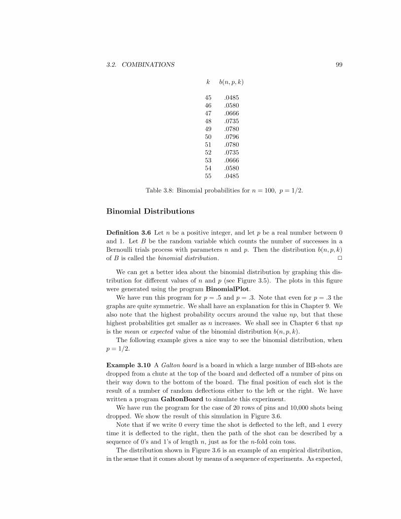
3.2. COMBINATIONS 99
k b(n, p, k)
45 .048546 .058047 .066648 .073549 .078050 .079651 .078052 .073553 .066654 .058055 .0485
Table 3.8: Binomial probabilities for n = 100, p = 1/2.
Binomial Distributions
Definition 3.6 Let n be a positive integer, and let p be a real number between 0and 1. Let B be the random variable which counts the number of successes in aBernoulli trials process with parameters n and p. Then the distribution b(n, p, k)of B is called the binomial distribution. 2
We can get a better idea about the binomial distribution by graphing this dis-tribution for different values of n and p (see Figure 3.5). The plots in this figurewere generated using the program BinomialPlot.
We have run this program for p = .5 and p = .3. Note that even for p = .3 thegraphs are quite symmetric. We shall have an explanation for this in Chapter 9. Wealso note that the highest probability occurs around the value np, but that thesehighest probabilities get smaller as n increases. We shall see in Chapter 6 that npis the mean or expected value of the binomial distribution b(n, p, k).
The following example gives a nice way to see the binomial distribution, whenp = 1/2.
Example 3.10 A Galton board is a board in which a large number of BB-shots aredropped from a chute at the top of the board and deflected off a number of pins ontheir way down to the bottom of the board. The final position of each slot is theresult of a number of random deflections either to the left or the right. We havewritten a program GaltonBoard to simulate this experiment.
We have run the program for the case of 20 rows of pins and 10,000 shots beingdropped. We show the result of this simulation in Figure 3.6.
Note that if we write 0 every time the shot is deflected to the left, and 1 everytime it is deflected to the right, then the path of the shot can be described by asequence of 0’s and 1’s of length n, just as for the n-fold coin toss.
The distribution shown in Figure 3.6 is an example of an empirical distribution,in the sense that it comes about by means of a sequence of experiments. As expected,

100 CHAPTER 3. COMBINATORICS
0 20 40 60 80 100 120
0
0.025
0.05
0.075
0.1
0.125
0.15
0 20 40 60 80 100
0.02
0.04
0.06
0.08
0.1
0.12 p = .5
n = 40
n = 80
n = 160
n = 30
n = 120
n = 270
p = .3
0
Figure 3.5: Binomial distributions.
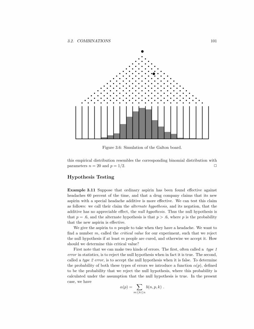
3.2. COMBINATIONS 101
Figure 3.6: Simulation of the Galton board.
this empirical distribution resembles the corresponding binomial distribution withparameters n = 20 and p = 1/2. 2
Hypothesis Testing
Example 3.11 Suppose that ordinary aspirin has been found effective againstheadaches 60 percent of the time, and that a drug company claims that its newaspirin with a special headache additive is more effective. We can test this claimas follows: we call their claim the alternate hypothesis, and its negation, that theadditive has no appreciable effect, the null hypothesis. Thus the null hypothesis isthat p = .6, and the alternate hypothesis is that p > .6, where p is the probabilitythat the new aspirin is effective.
We give the aspirin to n people to take when they have a headache. We want tofind a number m, called the critical value for our experiment, such that we rejectthe null hypothesis if at least m people are cured, and otherwise we accept it. Howshould we determine this critical value?
First note that we can make two kinds of errors. The first, often called a type 1error in statistics, is to reject the null hypothesis when in fact it is true. The second,called a type 2 error, is to accept the null hypothesis when it is false. To determinethe probability of both these types of errors we introduce a function α(p), definedto be the probability that we reject the null hypothesis, where this probability iscalculated under the assumption that the null hypothesis is true. In the presentcase, we have
α(p) =∑
m≤k≤nb(n, p, k) .

102 CHAPTER 3. COMBINATORICS
Note that α(.6) is the probability of a type 1 error, since this is the probabilityof a high number of successes for an ineffective additive. So for a given n we wantto choose m so as to make α(.6) quite small, to reduce the likelihood of a type 1error. But as m increases above the most probable value np = .6n, α(.6), beingthe upper tail of a binomial distribution, approaches 0. Thus increasing m makesa type 1 error less likely.
Now suppose that the additive really is effective, so that p is appreciably greaterthan .6; say p = .8. (This alternative value of p is chosen arbitrarily; the followingcalculations depend on this choice.) Then choosing m well below np = .8n willincrease α(.8), since now α(.8) is all but the lower tail of a binomial distribution.Indeed, if we put β(.8) = 1− α(.8), then β(.8) gives us the probability of a type 2error, and so decreasing m makes a type 2 error less likely.
The manufacturer would like to guard against a type 2 error, since if such anerror is made, then the test does not show that the new drug is better, when infact it is. If the alternative value of p is chosen closer to the value of p given inthe null hypothesis (in this case p = .6), then for a given test population, thevalue of β will increase. So, if the manufacturer’s statistician chooses an alternativevalue for p which is close to the value in the null hypothesis, then it will be anexpensive proposition (i.e., the test population will have to be large) to reject thenull hypothesis with a small value of β.
What we hope to do then, for a given test population n, is to choose a valueof m, if possible, which makes both these probabilities small. If we make a type 1error we end up buying a lot of essentially ordinary aspirin at an inflated price; atype 2 error means we miss a bargain on a superior medication. Let us say thatwe want our critical number m to make each of these undesirable cases less than 5percent probable.
We write a program PowerCurve to plot, for n = 100 and selected values of m,the function α(p), for p ranging from .4 to 1. The result is shown in Figure 3.7. Weinclude in our graph a box (in dotted lines) from .6 to .8, with bottom and top atheights .05 and .95. Then a value for m satisfies our requirements if and only if thegraph of α enters the box from the bottom, and leaves from the top (why?—whichis the type 1 and which is the type 2 criterion?). As m increases, the graph of αmoves to the right. A few experiments have shown us that m = 69 is the smallestvalue for m that thwarts a type 1 error, while m = 73 is the largest which thwarts atype 2. So we may choose our critical value between 69 and 73. If we’re more intenton avoiding a type 1 error we favor 73, and similarly we favor 69 if we regard atype 2 error as worse. Of course, the drug company may not be happy with havingas much as a 5 percent chance of an error. They might insist on having a 1 percentchance of an error. For this we would have to increase the number n of trials (seeExercise 28). 2
Binomial Expansion
We next remind the reader of an application of the binomial coefficients to algebra.This is the binomial expansion, from which we get the term binomial coefficient.

3.2. COMBINATIONS 103
.4 1.5 .6 .7 .8 .9 1 .0
1.0
.1
.2
.3
.4
.5
.6
.7
.8
.9
1.0
.4 1.5 .6 .7 .8 .9 1 .0
1.0
.1
.2
.3
.4
.5
.6
.7
.8
.9
1.0
Figure 3.7: The power curve.
Theorem 3.7 (Binomial Theorem) The quantity (a + b)n can be expressed inthe form
(a+ b)n =n∑j=0
(n
j
)ajbn−j .
Proof. To see that this expansion is correct, write
(a+ b)n = (a+ b)(a+ b) · · · (a+ b) .
When we multiply this out we will have a sum of terms each of which results froma choice of an a or b for each of n factors. When we choose j a’s and (n − j) b’s,we obtain a term of the form ajbn−j . To determine such a term, we have to specifyj of the n terms in the product from which we choose the a. This can be done in(nj
)ways. Thus, collecting these terms in the sum contributes a term
(nj
)ajbn−j . 2
For example, we have
(a+ b)0 = 1
(a+ b)1 = a+ b
(a+ b)2 = a2 + 2ab+ b2
(a+ b)3 = a3 + 3a2b+ 3ab2 + b3 .
We see here that the coefficients of successive powers do indeed yield Pascal’s tri-angle.
Corollary 3.1 The sum of the elements in the nth row of Pascal’s triangle is 2n.If the elements in the nth row of Pascal’s triangle are added with alternating signs,the sum is 0.

104 CHAPTER 3. COMBINATORICS
Proof. The first statement in the corollary follows from the fact that
2n = (1 + 1)n =(n
0
)+(n
1
)+(n
2
)+ · · ·+
(n
n
),
and the second from the fact that
0 = (1− 1)n =(n
0
)−(n
1
)+(n
2
)− · · ·+ (−1)n
(n
n
).
2
The first statement of the corollary tells us that the number of subsets of a setof n elements is 2n. We shall use the second statement in our next application ofthe binomial theorem.
We have seen that, when A and B are any two events (cf. Section 1.2),
P (A ∪B) = P (A) + P (B)− P (A ∩B).
We now extend this theorem to a more general version, which will enable us to findthe probability that at least one of a number of events occurs.
Inclusion-Exclusion Principle
Theorem 3.8 Let P be a probability measure on a sample space Ω, and letA1, A2, . . . , An be a finite set of events. Then
P (A1 ∪A2 ∪ · · · ∪An) =n∑i=1
P (Ai) −∑
1≤i<j≤nP (Ai ∩Aj)
+∑
1≤i<j<k≤nP (Ai ∩Aj ∩Ak)− · · · . (3.3)
That is, to find the probability that at least one of n events Ai occurs, first addthe probability of each event, then subtract the probabilities of all possible two-wayintersections, add the probability of all three-way intersections, and so forth.
Proof. If the outcome ω occurs in at least one of the events Ai, its probability isadded exactly once by the left side of Equation 3.3. We must show that it is addedexactly once by the right side of Equation 3.3. Assume that ω is in exactly k of thesets. Then its probability is added k times in the first term, subtracted
(k2
)times in
the second, added(k3
)times in the third term, and so forth. Thus, the total number
of times that it is added is(k
1
)−(k
2
)+(k
3
)− · · · (−1)k−1
(k
k
).
But
0 = (1− 1)k =k∑j=0
(k
j
)(−1)j =
(k
0
)−
k∑j=1
(k
j
)(−1)j−1 .

3.2. COMBINATIONS 105
Hence,
1 =(k
0
)=
k∑j=1
(k
j
)(−1)j−1 .
If the outcome ω is not in any of the events Ai, then it is not counted on either sideof the equation. 2
Hat Check Problem
Example 3.12 We return to the hat check problem discussed in Section 3.1, thatis, the problem of finding the probability that a random permutation contains atleast one fixed point. Recall that a permutation is a one-to-one map of a setA = a1, a2, . . . , an onto itself. Let Ai be the event that the ith element ai remainsfixed under this map. If we require that ai is fixed, then the map of the remainingn−1 elements provides an arbitrary permutation of (n−1) objects. Since there are(n − 1)! such permutations, P (Ai) = (n − 1)!/n! = 1/n. Since there are n choicesfor ai, the first term of Equation 3.3 is 1. In the same way, to have a particularpair (ai, aj) fixed, we can choose any permutation of the remaining n− 2 elements;there are (n− 2)! such choices and thus
P (Ai ∩Aj) =(n− 2)!n!
=1
n(n− 1).
The number of terms of this form in the right side of Equation 3.3 is(n
2
)=n(n− 1)
2!.
Hence, the second term of Equation 3.3 is
−n(n− 1)2!
· 1n(n− 1)
= − 12!.
Similarly, for any specific three events Ai, Aj , Ak,
P (Ai ∩Aj ∩Ak) =(n− 3)!n!
=1
n(n− 1)(n− 2),
and the number of such terms is(n
3
)=n(n− 1)(n− 2)
3!,
making the third term of Equation 3.3 equal to 1/3!. Continuing in this way, weobtain
P (at least one fixed point) = 1− 12!
+13!− · · · (−1)n−1 1
n!and
P (no fixed point) =12!− 1
3!+ · · · (−1)n
1n!
.

106 CHAPTER 3. COMBINATORICS
Probability that no onen gets his own hat back3 .3333334 .3755 .3666676 .3680567 .3678578 .3678829 .367879
10 .367879
Table 3.9: Hat check problem.
From calculus we learn that
ex = 1 + x+12!x2 +
13!x3 + · · ·+ 1
n!xn + · · · .
Thus, if x = −1, we have
e−1 =12!− 1
3!+ · · ·+ (−1)n
n!+ · · ·
= .3678794 .
Therefore, the probability that there is no fixed point, i.e., that none of the n peoplegets his own hat back, is equal to the sum of the first n terms in the expression fore−1. This series converges very fast. Calculating the partial sums for n = 3 to 10gives the data in Table 3.9.
After n = 9 the probabilities are essentially the same to six significant figures.Interestingly, the probability of no fixed point alternately increases and decreasesas n increases. Finally, we note that our exact results are in good agreement withour simulations reported in the previous section. 2
Choosing a Sample Space
We now have some of the tools needed to accurately describe sample spaces andto assign probability functions to those sample spaces. Nevertheless, in some cases,the description and assignment process is somewhat arbitrary. Of course, it is tobe hoped that the description of the sample space and the subsequent assignmentof a probability function will yield a model which accurately predicts what wouldhappen if the experiment were actually carried out. As the following examples show,there are situations in which “reasonable” descriptions of the sample space do notproduce a model which fits the data.
In Feller’s book,14 a pair of models is given which describe arrangements ofcertain kinds of elementary particles, such as photons and protons. It turns out thatexperiments have shown that certain types of elementary particles exhibit behavior
14W. Feller, Introduction to Probability Theory and Its Applications vol. 1, 3rd ed. (New York:John Wiley and Sons, 1968), p. 41
3.2. COMBINATIONS 107
which is accurately described by one model, called “Bose-Einstein statistics,” whileother types of elementary particles can be modelled using “Fermi-Dirac statistics.”Feller says:
We have here an instructive example of the impossibility of selecting orjustifying probability models by a priori arguments. In fact, no purereasoning could tell that photons and protons would not obey the sameprobability laws.
We now give some examples of this description and assignment process.
Example 3.13 In the quantum mechanical model of the helium atom, variousparameters can be used to classify the energy states of the atom. In the tripletspin state (S = 1) with orbital angular momentum 1 (L = 1), there are threepossibilities, 0, 1, or 2, for the total angular momentum (J). (It is not assumed thatthe reader knows what any of this means; in fact, the example is more illustrativeif the reader does not know anything about quantum mechanics.) We would liketo assign probabilities to the three possibilities for J . The reader is undoubtedlyresisting the idea of assigning the probability of 1/3 to each of these outcomes. Sheshould now ask herself why she is resisting this assignment. The answer is probablybecause she does not have any “intuition” (i.e., experience) about the way in whichhelium atoms behave. In fact, in this example, the probabilities 1/9, 3/9, and5/9 are assigned by the theory. The theory gives these assignments because thesefrequencies were observed in experiments and further parameters were developed inthe theory to allow these frequencies to be predicted. 2
Example 3.14 Suppose two pennies are flipped once each. There are several “rea-sonable” ways to describe the sample space. One way is to count the number ofheads in the outcome; in this case, the sample space can be written 0, 1, 2. An-other description of the sample space is the set of all ordered pairs of H’s and T ’s,i.e.,
(H,H), (H,T ), (T,H), (T, T ).Both of these descriptions are accurate ones, but it is easy to see that (at most) oneof these, if assigned a constant probability function, can claim to accurately modelreality. In this case, as opposed to the preceding example, the reader will probablysay that the second description, with each outcome being assigned a probability of1/4, is the “right” description. This conviction is due to experience; there is noproof that this is the way reality works. 2
The reader is also referred to Exercise 26 for another example of this process.
Historical Remarks
The binomial coefficients have a long and colorful history leading up to Pascal’sTreatise on the Arithmetical Triangle,15 where Pascal developed many important
15B. Pascal, Traite du Triangle Arithmetique (Paris: Desprez, 1665).

108 CHAPTER 3. COMBINATORICS
1 1 1 1 1 1 1 1 1 11 2 3 4 5 6 7 8 91 3 6 10 15 21 28 361 4 10 20 35 56 841 5 15 35 70 1261 6 21 56 1261 7 28 841 8 361 91
Table 3.10: Pascal’s triangle.
natural numbers 1 2 3 4 5 6 7 8 9triangular numbers 1 3 6 10 15 21 28 36 45tetrahedral numbers 1 4 10 20 35 56 84 120 165
Table 3.11: Figurate numbers.
properties of these numbers. This history is set forth in the book Pascal’s Arith-metical Triangle by A. W. F. Edwards.16 Pascal wrote his triangle in the formshown in Table 3.10.
Edwards traces three different ways that the binomial coefficients arose. Herefers to these as the figurate numbers, the combinatorial numbers, and the binomialnumbers. They are all names for the same thing (which we have called binomialcoefficients) but that they are all the same was not appreciated until the sixteenthcentury.
The figurate numbers date back to the Pythagorean interest in number pat-terns around 540 BC. The Pythagoreans considered, for example, triangular patternsshown in Figure 3.8. The sequence of numbers
1, 3, 6, 10, . . .
obtained as the number of points in each triangle are called triangular numbers.From the triangles it is clear that the nth triangular number is simply the sum ofthe first n integers. The tetrahedral numbers are the sums of the triangular numbersand were obtained by the Greek mathematicians Theon and Nicomachus at thebeginning of the second century BC. The tetrahedral number 10, for example, hasthe geometric representation shown in Figure 3.9. The first three types of figuratenumbers can be represented in tabular form as shown in Table 3.11.
These numbers provide the first four rows of Pascal’s triangle, but the table wasnot to be completed in the West until the sixteenth century.
In the East, Hindu mathematicians began to encounter the binomial coefficientsin combinatorial problems. Bhaskara in his Lilavati of 1150 gave a rule to find the
16A. W. F. Edwards, Pascal’s Arithmetical Triangle (London: Griffin, 1987).

3.2. COMBINATIONS 109
1 3 6 10
Figure 3.8: Pythagorean triangular patterns.
Figure 3.9: Geometric representation of the tetrahedral number 10.

110 CHAPTER 3. COMBINATORICS
1112 2213 23 3314 24 34 4415 25 35 45 5516 26 36 46 56 66
Table 3.12: Outcomes for the roll of two dice.
number of medicinal preparations using 1, 2, 3, 4, 5, or 6 possible ingredients.17 Hisrule is equivalent to our formula (
n
r
)=
(n)rr!
.
The binomial numbers as coefficients of (a+ b)n appeared in the works of math-ematicians in China around 1100. There are references about this time to “thetabulation system for unlocking binomial coefficients.” The triangle to provide thecoefficients up to the eighth power is given by Chu Shih-chieh in a book writtenaround 1303 (see Figure 3.10).18 The original manuscript of Chu’s book has beenlost, but copies have survived. Edwards notes that there is an error in this copy ofChu’s triangle. Can you find it? (Hint : Two numbers which should be equal arenot.) Other copies do not show this error.
The first appearance of Pascal’s triangle in the West seems to have come fromcalculations of Tartaglia in calculating the number of possible ways that n dicemight turn up.19 For one die the answer is clearly 6. For two dice the possibilitiesmay be displayed as shown in Table 3.12.
Displaying them this way suggests the sixth triangular number 1 + 2 + 3 + 4 +5 + 6 = 21 for the throw of 2 dice. Tartaglia “on the first day of Lent, 1523, inVerona, having thought about the problem all night,”20 realized that the extensionof the figurate table gave the answers for n dice. The problem had suggested itselfto Tartaglia from watching people casting their own horoscopes by means of a Bookof Fortune, selecting verses by a process which included noting the numbers on thefaces of three dice. The 56 ways that three dice can fall were set out on each page.The way the numbers were written in the book did not suggest the connection withfigurate numbers, but a method of enumeration similar to the one we used for 2dice does. Tartaglia’s table was not published until 1556.
A table for the binomial coefficients was published in 1554 by the German mathe-matician Stifel.21 Pascal’s triangle appears also in Cardano’s Opus novum of 1570.22
17ibid., p. 27.18J. Needham, Science and Civilization in China, vol. 3 (New York: Cambridge University
Press, 1959), p. 135.19N. Tartaglia, General Trattato di Numeri et Misure (Vinegia, 1556).20Quoted in Edwards, op. cit., p. 37.21M. Stifel, Arithmetica Integra (Norimburgae, 1544).22G. Cardano, Opus Novum de Proportionibus Numerorum (Basilea, 1570).

3.2. COMBINATIONS 111
Figure 3.10: Chu Shih-chieh’s triangle. [From J. Needham, Science and Civilizationin China, vol. 3 (New York: Cambridge University Press, 1959), p. 135. Reprintedwith permission.]
112 CHAPTER 3. COMBINATORICS
Cardano was interested in the problem of finding the number of ways to choose robjects out of n. Thus by the time of Pascal’s work, his triangle had appeared asa result of looking at the figurate numbers, the combinatorial numbers, and thebinomial numbers, and the fact that all three were the same was presumably prettywell understood.
Pascal’s interest in the binomial numbers came from his letters with Fermatconcerning a problem known as the problem of points. This problem, and thecorrespondence between Pascal and Fermat, were discussed in Chapter 1. Thereader will recall that this problem can be described as follows: Two players A andB are playing a sequence of games and the first player to win n games wins thematch. It is desired to find the probability that A wins the match at a time whenA has won a games and B has won b games. (See Exercises 4.1.40-4.1.42.)
Pascal solved the problem by backward induction, much the way we would dotoday in writing a computer program for its solution. He referred to the combina-torial method of Fermat which proceeds as follows: If A needs c games and B needsd games to win, we require that the players continue to play until they have playedc+ d− 1 games. The winner in this extended series will be the same as the winnerin the original series. The probability that A wins in the extended series and hencein the original series is
c+d−1∑r=c
12c+d−1
(c+ d− 1
r
).
Even at the time of the letters Pascal seemed to understand this formula.Suppose that the first player to win n games wins the match, and suppose that
each player has put up a stake of x. Pascal studied the value of winning a particulargame. By this he meant the increase in the expected winnings of the winner of theparticular game under consideration. He showed that the value of the first game is
1 · 3 · 5 · . . . · (2n− 1)2 · 4 · 6 · . . . · (2n)
x .
His proof of this seems to use Fermat’s formula and the fact that the above ratio ofproducts of odd to products of even numbers is equal to the probability of exactlyn heads in 2n tosses of a coin. (See Exercise 39.)
Pascal presented Fermat with the table shown in Table 3.13. He states:
You will see as always, that the value of the first game is equal to thatof the second which is easily shown by combinations. You will see, inthe same way, that the numbers in the first line are always increasing;so also are those in the second; and those in the third. But those in thefourth line are decreasing, and those in the fifth, etc. This seems odd.23
The student can pursue this question further using the computer and Pascal’sbackward iteration method for computing the expected payoff at any point in theseries.
23F. N. David, op. cit., p. 235.

3.2. COMBINATIONS 113
if each one staken 256 inFrom my opponent’s 256 6 5 4 3 2 1positions I get, for the games games games games games games
1st game 63 70 80 96 128 2562nd game 63 70 80 96 1283rd game 56 60 64 644th game 42 40 325th game 24 166th game 8
Table 3.13: Pascal’s solution for the problem of points.
In his treatise, Pascal gave a formal proof of Fermat’s combinatorial formula aswell as proofs of many other basic properties of binomial numbers. Many of hisproofs involved induction and represent some of the first proofs by this method.His book brought together all the different aspects of the numbers in the Pascaltriangle as known in 1654, and, as Edwards states, “That the Arithmetical Triangleshould bear Pascal’s name cannot be disputed.”24
The first serious study of the binomial distribution was undertaken by JamesBernoulli in his Ars Conjectandi published in 1713.25 We shall return to this workin the historical remarks in Chapter 8.
Exercises
1 Compute the following:
(a)(
63
)(b) b(5, .2, 4)
(c)(
72
)(d)
(2626
)(e) b(4, .2, 3)
(f)(
62
)(g)
(109
)(h) b(8, .3, 5)
2 In how many ways can we choose five people from a group of ten to form acommittee?
3 How many seven-element subsets are there in a set of nine elements?
4 Using the relation Equation 3.1 write a program to compute Pascal’s triangle,putting the results in a matrix. Have your program print the triangle forn = 10.
24A. W. F. Edwards, op. cit., p. ix.25J. Bernoulli, Ars Conjectandi (Basil: Thurnisiorum, 1713).

114 CHAPTER 3. COMBINATORICS
5 Use the program BinomialProbabilities to find the probability that, in 100tosses of a fair coin, the number of heads that turns up lies between 35 and65, between 40 and 60, and between 45 and 55.
6 Charles claims that he can distinguish between beer and ale 75 percent of thetime. Ruth bets that he cannot and, in fact, just guesses. To settle this, a betis made: Charles is to be given ten small glasses, each having been filled withbeer or ale, chosen by tossing a fair coin. He wins the bet if he gets seven ormore correct. Find the probability that Charles wins if he has the ability thathe claims. Find the probability that Ruth wins if Charles is guessing.
7 Show that
b(n, p, j) =p
q
(n− j + 1
j
)b(n, p, j − 1) ,
for j ≥ 1. Use this fact to determine the value or values of j which giveb(n, p, j) its greatest value. Hint : Consider the successive ratios as j increases.
8 A die is rolled 30 times. What is the probability that a 6 turns up exactly 5times? What is the most probable number of times that a 6 will turn up?
9 Find integers n and r such that the following equation is true:(135
)+ 2(
136
)+(
137
)=(n
r
).
10 In a ten-question true-false exam, find the probability that a student gets agrade of 70 percent or better by guessing. Answer the same question if thetest has 30 questions, and if the test has 50 questions.
11 A restaurant offers apple and blueberry pies and stocks an equal number ofeach kind of pie. Each day ten customers request pie. They choose, withequal probabilities, one of the two kinds of pie. How many pieces of each kindof pie should the owner provide so that the probability is about .95 that eachcustomer gets the pie of his or her own choice?
12 A poker hand is a set of 5 cards randomly chosen from a deck of 52 cards.Find the probability of a
(a) royal flush (ten, jack, queen, king, ace in a single suit).
(b) straight flush (five in a sequence in a single suit, but not a royal flush).
(c) four of a kind (four cards of the same face value).
(d) full house (one pair and one triple, each of the same face value).
(e) flush (five cards in a single suit but not a straight or royal flush).
(f) straight (five cards in a sequence, not all the same suit). (Note that instraights, an ace counts high or low.)
13 If a set has 2n elements, show that it has more subsets with n elements thanwith any other number of elements.
3.2. COMBINATIONS 115
14 Let b(2n, .5, n) be the probability that in 2n tosses of a fair coin exactly n headsturn up. Using Stirling’s formula (Theorem 3.3), show that b(2n, .5, n) ∼1/√πn. Use the program BinomialProbabilities to compare this with the
exact value for n = 10 to 25.
15 A baseball player, Smith, has a batting average of .300 and in a typical gamecomes to bat three times. Assume that Smith’s hits in a game can be consid-ered to be a Bernoulli trials process with probability .3 for success. Find theprobability that Smith gets 0, 1, 2, and 3 hits.
16 The Siwash University football team plays eight games in a season, winningthree, losing three, and ending two in a tie. Show that the number of waysthat this can happen is (
83
)(53
)=
8!3! 3! 2!
.
17 Using the technique of Exercise 16, show that the number of ways that onecan put n different objects into three boxes with a in the first, b in the second,and c in the third is n!/(a! b! c!).
18 Baumgartner, Prosser, and Crowell are grading a calculus exam. There is atrue-false question with ten parts. Baumgartner notices that one student hasonly two out of the ten correct and remarks, “The student was not even brightenough to have flipped a coin to determine his answers.” “Not so clear,” saysProsser. “With 340 students I bet that if they all flipped coins to determinetheir answers there would be at least one exam with two or fewer answerscorrect.” Crowell says, “I’m with Prosser. In fact, I bet that we should expectat least one exam in which no answer is correct if everyone is just guessing.”Who is right in all of this?
19 A gin hand consists of 10 cards from a deck of 52 cards. Find the probabilitythat a gin hand has
(a) all 10 cards of the same suit.
(b) exactly 4 cards in one suit and 3 in two other suits.
(c) a 4, 3, 2, 1, distribution of suits.
20 A six-card hand is dealt from an ordinary deck of cards. Find the probabilitythat:
(a) All six cards are hearts.
(b) There are three aces, two kings, and one queen.
(c) There are three cards of one suit and three of another suit.
21 A lady wishes to color her fingernails on one hand using at most two of thecolors red, yellow, and blue. How many ways can she do this?
116 CHAPTER 3. COMBINATORICS
22 How many ways can six indistinguishable letters be put in three mail boxes?Hint : One representation of this is given by a sequence |LL|L|LLL| where the|’s represent the partitions for the boxes and the L’s the letters. Any possibleway can be so described. Note that we need two bars at the ends and theremaining two bars and the six L’s can be put in any order.
23 Using the method for the hint in Exercise 22, show that r indistinguishableobjects can be put in n boxes in(
n+ r − 1n− 1
)=(n+ r − 1
r
)different ways.
24 A travel bureau estimates that when 20 tourists go to a resort with ten hotelsthey distribute themselves as if the bureau were putting 20 indistinguishableobjects into ten distinguishable boxes. Assuming this model is correct, findthe probability that no hotel is left vacant when the first group of 20 touristsarrives.
25 An elevator takes on six passengers and stops at ten floors. We can assigntwo different equiprobable measures for the ways that the passengers are dis-charged: (a) we consider the passengers to be distinguishable or (b) we con-sider them to be indistinguishable (see Exercise 23 for this case). For eachcase, calculate the probability that all the passengers get off at different floors.
26 You are playing heads or tails with Prosser but you suspect that his coin isunfair. Von Neumann suggested that you proceed as follows: Toss Prosser’scoin twice. If the outcome is HT call the result win. if it is TH call the resultlose. If it is TT or HH ignore the outcome and toss Prosser’s coin twice again.Keep going until you get either an HT or a TH and call the result win or losein a single play. Repeat this procedure for each play. Assume that Prosser’scoin turns up heads with probability p.
(a) Find the probability of HT, TH, HH, TT with two tosses of Prosser’scoin.
(b) Using part (a), show that the probability of a win on any one play is 1/2,no matter what p is.
27 John claims that he has extrasensory powers and can tell which of two symbolsis on a card turned face down (see Example 3.11). To test his ability he isasked to do this for a sequence of trials. Let the null hypothesis be that he isjust guessing, so that the probability is 1/2 of his getting it right each time,and let the alternative hypothesis be that he can name the symbol correctlymore than half the time. Devise a test with the property that the probabilityof a type 1 error is less than .05 and the probability of a type 2 error is lessthan .05 if John can name the symbol correctly 75 percent of the time.

3.2. COMBINATIONS 117
28 In Example 3.11 assume the alternative hypothesis is that p = .8 and that itis desired to have the probability of each type of error less than .01. Use theprogram PowerCurve to determine values of n and m that will achieve this.Choose n as small as possible.
29 A drug is assumed to be effective with an unknown probability p. To estimatep the drug is given to n patients. It is found to be effective for m patients.The method of maximum likelihood for estimating p states that we shouldchoose the value for p that gives the highest probability of getting what wegot on the experiment. Assuming that the experiment can be considered as aBernoulli trials process with probability p for success, show that the maximumlikelihood estimate for p is the proportion m/n of successes.
30 Recall that in the World Series the first team to win four games wins theseries. The series can go at most seven games. Assume that the Red Soxand the Mets are playing the series. Assume that the Mets win each gamewith probability p. Fermat observed that even though the series might not goseven games, the probability that the Mets win the series is the same as theprobability that they win four or more game in a series that was forced to goseven games no matter who wins the individual games.
(a) Using the program PowerCurve of Example 3.11 find the probabilitythat the Mets win the series for the cases p = .5, p = .6, p = .7.
(b) Assume that the Mets have probability .6 of winning each game. Usethe program PowerCurve to find a value of n so that, if the series goesto the first team to win more than half the games, the Mets will have a95 percent chance of winning the series. Choose n as small as possible.
31 Each of the four engines on an airplane functions correctly on a given flightwith probability .99, and the engines function independently of each other.Assume that the plane can make a safe landing if at least two of its enginesare functioning correctly. What is the probability that the engines will allowfor a safe landing?
32 A small boy is lost coming down Mount Washington. The leader of the searchteam estimates that there is a probability p that he came down on the eastside and a probability 1 − p that he came down on the west side. He has npeople in his search team who will search independently and, if the boy ison the side being searched, each member will find the boy with probabilityu. Determine how he should divide the n people into two groups to searchthe two sides of the mountain so that he will have the highest probability offinding the boy. How does this depend on u?
*33 2n balls are chosen at random from a total of 2n red balls and 2n blue balls.Find a combinatorial expression for the probability that the chosen balls areequally divided in color. Use Stirling’s formula to estimate this probability.

118 CHAPTER 3. COMBINATORICS
Using BinomialProbabilities, compare the exact value with Stirling’s ap-proximation for n = 20.
34 Assume that every time you buy a box of Wheaties, you receive one of thepictures of the n players on the New York Yankees. Over a period of time,you buy m ≥ n boxes of Wheaties.
(a) Use Theorem 3.8 to show that the probability that you get all n picturesis
1 −(n
1
)(n− 1n
)m+(n
2
)(n− 2n
)m− · · ·
+ (−1)n−1
(n
n− 1
)(1n
)m.
Hint : Let Ek be the event that you do not get the kth player’s picture.
(b) Write a computer program to compute this probability. Use this programto find, for given n, the smallest value of m which will give probability≥ .5 of getting all n pictures. Consider n = 50, 100, and 150 and showthat m = n logn + n log 2 is a good estimate for the number of boxesneeded. (For a derivation of this estimate, see Feller.26)
*35 Prove the following binomial identity(2nn
)=
n∑j=0
(n
j
)2
.
Hint : Consider an urn with n red balls and n blue balls inside. Show thateach side of the equation equals the number of ways to choose n balls fromthe urn.
36 Let j and n be positive integers, with j ≤ n. An experiment consists ofchoosing, at random, a j-tuple of positive integers whose sum is at most n.
(a) Find the size of the sample space. Hint : Consider n indistinguishableballs placed in a row. Place j markers between consecutive pairs of balls,with no two markers between the same pair of balls. (We also allow oneof the n markers to be placed at the end of the row of balls.) Show thatthere is a 1-1 correspondence between the set of possible positions forthe markers and the set of j-tuples whose size we are trying to count.
(b) Find the probability that the j-tuple selected contains at least one 1.
37 Let n (mod m) denote the remainder when the integer n is divided by theinteger m. Write a computer program to compute the numbers
(nj
)(mod m)
where(nj
)is a binomial coefficient and m is an integer. You can do this by
using the recursion relations for generating binomial coefficients, doing all the26W. Feller, Introduction to Probability Theory and its Applications, vol. I, 3rd ed. (New York:
John Wiley & Sons, 1968), p. 106.

3.2. COMBINATIONS 119
arithmetic using the basic function mod(n,m). Try to write your program tomake as large a table as possible. Run your program for the cases m = 2 to 7.Do you see any patterns? In particular, for the case m = 2 and n a powerof 2, verify that all the entries in the (n− 1)st row are 1. (The correspondingbinomial numbers are odd.) Use your pictures to explain why this is true.
38 Lucas27 proved the following general result relating to Exercise 37. If p isany prime number, then
(nj
)(mod p) can be found as follows: Expand n
and j in base p as n = s0 + s1p + s2p2 + · · · + skp
k and j = r0 + r1p +r2p
2 + · · ·+ rkpk, respectively. (Here k is chosen large enough to represent all
numbers from 0 to n in base p using k digits.) Let s = (s0, s1, s2, . . . , sk) andr = (r0, r1, r2, . . . , rk). Then(
n
j
)(mod p) =
k∏i=0
(siri
)(mod p) .
For example, if p = 7, n = 12, and j = 9, then
12 = 5 · 70 + 1 · 71 ,
9 = 2 · 70 + 1 · 71 ,
so that
s = (5, 1) ,
r = (2, 1) ,
and this result states that(129
)(mod p) =
(52
)(11
)(mod 7) .
Since(
129
)= 220 = 3 (mod 7), and
(52
)= 10 = 3 (mod 7), we see that the
result is correct for this example.
Show that this result implies that, for p = 2, the (pk−1)st row of your trianglein Exercise 37 has no zeros.
39 Prove that the probability of exactly n heads in 2n tosses of a fair coin isgiven by the product of the odd numbers up to 2n− 1 divided by the productof the even numbers up to 2n.
40 Let n be a positive integer, and assume that j is a positive integer not exceed-ing n/2. Show that in Theorem 3.5, if one alternates the multiplications anddivisions, then all of the intermediate values in the calculation are integers.Show also that none of these intermediate values exceed the final value.
27E. Lucas, “Theorie des Functions Numeriques Simplement Periodiques,” American J. Math.,vol. 1 (1878), pp. 184-240, 289-321.

120 CHAPTER 3. COMBINATORICS
3.3 Card Shuffling
Much of this section is based upon an article by Brad Mann,28 which is an expositionof an article by David Bayer and Persi Diaconis.29
Riffle Shuffles
Given a deck of n cards, how many times must we shuffle it to make it “random”?Of course, the answer depends upon the method of shuffling which is used and whatwe mean by “random.” We shall begin the study of this question by considering astandard model for the riffle shuffle.
We begin with a deck of n cards, which we will assume are labelled in increasingorder with the integers from 1 to n. A riffle shuffle consists of a cut of the deck intotwo stacks and an interleaving of the two stacks. For example, if n = 6, the initialordering is (1, 2, 3, 4, 5, 6), and a cut might occur between cards 2 and 3. This givesrise to two stacks, namely (1, 2) and (3, 4, 5, 6). These are interleaved to form anew ordering of the deck. For example, these two stacks might form the ordering(1, 3, 4, 2, 5, 6). In order to discuss such shuffles, we need to assign a probabilitymeasure to the set of all possible shuffles. There are several reasonable ways inwhich this can be done. We will give several different assignment strategies, andshow that they are equivalent. (This does not mean that this assignment is theonly reasonable one.) First, we assign the binomial probability b(n, 1/2, k) to theevent that the cut occurs after the kth card. Next, we assume that all possibleinterleavings, given a cut, are equally likely. Thus, to complete the assignmentof probabilities, we need to determine the number of possible interleavings of twostacks of cards, with k and n− k cards, respectively.
We begin by writing the second stack in a line, with spaces in between eachpair of consecutive cards, and with spaces at the beginning and end (so there aren − k + 1 spaces). We choose, with replacement, k of these spaces, and place thecards from the first stack in the chosen spaces. This can be done in(
n
k
)ways. Thus, the probability of a given interleaving should be
1(nk
) .Next, we note that if the new ordering is not the identity ordering, it is the
result of a unique cut-interleaving pair. If the new ordering is the identity, it is theresult of any one of n+ 1 cut-interleaving pairs.
We define a rising sequence in an ordering to be a maximal subsequence ofconsecutive integers in increasing order. For example, in the ordering
(2, 3, 5, 1, 4, 7, 6) ,28B. Mann, “How Many Times Should You Shuffle a Deck of Cards?”, UMAP Journal , vol. 15,
no. 4 (1994), pp. 303–331.29D. Bayer and P. Diaconis, “Trailing the Dovetail Shuffle to its Lair,” Annals of Applied Prob-
ability, vol. 2, no. 2 (1992), pp. 294–313.

3.3. CARD SHUFFLING 121
there are 4 rising sequences; they are (1), (2, 3, 4), (5, 6), and (7). It is easy to seethat an ordering is the result of a riffle shuffle applied to the identity ordering ifand only if it has no more than two rising sequences. (If the ordering has two risingsequences, then these rising sequences correspond to the two stacks induced by thecut, and if the ordering has one rising sequence, then it is the identity ordering.)Thus, the sample space of orderings obtained by applying a riffle shuffle to theidentity ordering is naturally described as the set of all orderings with at most tworising sequences.
It is now easy to assign a probability measure to this sample space. Each orderingwith two rising sequences is assigned the value
b(n, 1/2, k)(nk
) =12n
,
and the identity ordering is assigned the value
n+ 12n
.
There is another way to view a riffle shuffle. We can imagine starting with adeck cut into two stacks as before, with the same probabilities assignment as beforei.e., the binomial distribution. Once we have the two stacks, we take cards, one byone, off of the bottom of the two stacks, and place them onto one stack. If thereare k1 and k2 cards, respectively, in the two stacks at some point in this process,then we make the assumption that the probabilities that the next card to be takencomes from a given stack is proportional to the current stack size. This implies thatthe probability that we take the next card from the first stack equals
k1
k1 + k2,
and the corresponding probability for the second stack is
k2
k1 + k2.
We shall now show that this process assigns the uniform probability to each of thepossible interleavings of the two stacks.
Suppose, for example, that an interleaving came about as the result of choosingcards from the two stacks in some order. The probability that this result occurredis the product of the probabilities at each point in the process, since the choiceof card at each point is assumed to be independent of the previous choices. Eachfactor of this product is of the form
kik1 + k2
,
where i = 1 or 2, and the denominator of each factor equals the number of cards leftto be chosen. Thus, the denominator of the probability is just n!. At the momentwhen a card is chosen from a stack that has i cards in it, the numerator of the

122 CHAPTER 3. COMBINATORICS
corresponding factor in the probability is i, and the number of cards in this stackdecreases by 1. Thus, the numerator is seen to be k!(n− k)!, since all cards in bothstacks are eventually chosen. Therefore, this process assigns the probability
1(nk
)to each possible interleaving.
We now turn to the question of what happens when we riffle shuffle s times. Itshould be clear that if we start with the identity ordering, we obtain an orderingwith at most 2s rising sequences, since a riffle shuffle creates at most two risingsequences from every rising sequence in the starting ordering. In fact, it is not hardto see that each such ordering is the result of s riffle shuffles. The question becomes,then, in how many ways can an ordering with r rising sequences come about byapplying s riffle shuffles to the identity ordering? In order to answer this question,we turn to the idea of an a-shuffle.
a-Shuffles
There are several ways to visualize an a-shuffle. One way is to imagine a creaturewith a hands who is given a deck of cards to riffle shuffle. The creature naturallycuts the deck into a stacks, and then riffles them together. (Imagine that!) Thus,the ordinary riffle shuffle is a 2-shuffle. As in the case of the ordinary 2-shuffle, weallow some of the stacks to have 0 cards. Another way to visualize an a-shuffle isto think about its inverse, called an a-unshuffle. This idea is described in the proofof the next theorem.
We will now show that an a-shuffle followed by a b-shuffle is equivalent to an ab-shuffle. This means, in particular, that s riffle shuffles in succession are equivalentto one 2s-shuffle. This equivalence is made precise by the following theorem.
Theorem 3.9 Let a and b be two positive integers. Let Sa,b be the set of all orderedpairs in which the first entry is an a-shuffle and the second entry is a b-shuffle. LetSab be the set of all ab-shuffles. Then there is a 1-1 correspondence between Sa,band Sab with the following property. Suppose that (T1, T2) corresponds to T3. IfT1 is applied to the identity ordering, and T2 is applied to the resulting ordering,then the final ordering is the same as the ordering that is obtained by applying T3
to the identity ordering.
Proof. The easiest way to describe the required correspondence is through the ideaof an unshuffle. An a-unshuffle begins with a deck of n cards. One by one, cards aretaken from the top of the deck and placed, with equal probability, on the bottomof any one of a stacks, where the stacks are labelled from 0 to a−1. After all of thecards have been distributed, we combine the stacks to form one stack by placingstack i on top of stack i+1, for 0 ≤ i ≤ a−1. It is easy to see that if one starts witha deck, there is exactly one way to cut the deck to obtain the a stacks generated bythe a-unshuffle, and with these a stacks, there is exactly one way to interleave them

3.3. CARD SHUFFLING 123
to obtain the deck in the order that it was in before the unshuffle was performed.Thus, this a-unshuffle corresponds to a unique a-shuffle, and this a-shuffle is theinverse of the original a-unshuffle.
If we apply an ab-unshuffle U3 to a deck, we obtain a set of ab stacks, whichare then combined, in order, to form one stack. We label these stacks with orderedpairs of integers, where the first coordinate is between 0 and a− 1, and the secondcoordinate is between 0 and b − 1. Then we label each card with the label of itsstack. The number of possible labels is ab, as required. Using this labelling, wecan describe how to find a b-unshuffle and an a-unshuffle, such that if these twounshuffles are applied in this order to the deck, we obtain the same set of ab stacksas were obtained by the ab-unshuffle.
To obtain the b-unshuffle U2, we sort the deck into b stacks, with the ith stackcontaining all of the cards with second coordinate i, for 0 ≤ i ≤ b− 1. Then thesestacks are combined to form one stack. The a-unshuffle U1 proceeds in the samemanner, except that the first coordinates of the labels are used. The resulting a
stacks are then combined to form one stack.The above description shows that the cards ending up on top are all those
labelled (0, 0). These are followed by those labelled (0, 1), (0, 2), . . . , (0, b −1), (1, 0), (1, 1), . . . , (a − 1, b − 1). Furthermore, the relative order of any pairof cards with the same labels is never altered. But this is exactly the same as anab-unshuffle, if, at the beginning of such an unshuffle, we label each of the cardswith one of the labels (0, 0), (0, 1), . . . , (0, b− 1), (1, 0), (1, 1), . . . , (a− 1, b− 1).This completes the proof. 2
In Figure 3.11, we show the labels for a 2-unshuffle of a deck with 10 cards.There are 4 cards with the label 0 and 6 cards with the label 1, so if the 2-unshuffleis performed, the first stack will have 4 cards and the second stack will have 6 cards.When this unshuffle is performed, the deck ends up in the identity ordering.
In Figure 3.12, we show the labels for a 4-unshuffle of the same deck (becausethere are four labels being used). This figure can also be regarded as an example ofa pair of 2-unshuffles, as described in the proof above. The first 2-unshuffle will usethe second coordinate of the labels to determine the stacks. In this case, the twostacks contain the cards whose values are
5, 1, 6, 2, 7 and 8, 9, 3, 4, 10 .
After this 2-unshuffle has been performed, the deck is in the order shown in Fig-ure 3.11, as the reader should check. If we wish to perform a 4-unshuffle on thedeck, using the labels shown, we sort the cards lexicographically, obtaining the fourstacks
1, 2, 3, 4, 5, 6, 7, and 8, 9, 10 .
When these stacks are combined, we once again obtain the identity ordering of thedeck. The point of the above theorem is that both sorting procedures always leadto the same initial ordering.

124 CHAPTER 3. COMBINATORICS
Figure 3.11: Before a 2-unshuffle.
Figure 3.12: Before a 4-unshuffle.

3.3. CARD SHUFFLING 125
Theorem 3.10 If D is any ordering that is the result of applying an a-shuffle andthen a b-shuffle to the identity ordering, then the probability assigned to D by thispair of operations is the same as the probability assigned to D by the process ofapplying an ab-shuffle to the identity ordering.
Proof. Call the sample space of a-shuffles Sa. If we label the stacks by the integersfrom 0 to a− 1, then each cut-interleaving pair, i.e., shuffle, corresponds to exactlyone n-digit base a integer, where the ith digit in the integer is the stack of whichthe ith card is a member. Thus, the number of cut-interleaving pairs is equal tothe number of n-digit base a integers, which is an. Of course, not all of thesepairs leads to different orderings. The number of pairs leading to a given orderingwill be discussed later. For our purposes it is enough to point out that it is thecut-interleaving pairs that determine the probability assignment.
The previous theorem shows that there is a 1-1 correspondence between Sa,b andSab. Furthermore, corresponding elements give the same ordering when applied tothe identity ordering. Given any ordering D, let m1 be the number of elementsof Sa,b which, when applied to the identity ordering, result in D. Let m2 be thenumber of elements of Sab which, when applied to the identity ordering, result in D.The previous theorem implies that m1 = m2. Thus, both sets assign the probability
m1
(ab)n
to D. This completes the proof. 2
Connection with the Birthday Problem
There is another point that can be made concerning the labels given to the cardsby the successive unshuffles. Suppose that we 2-unshuffle an n-card deck until thelabels on the cards are all different. It is easy to see that this process produceseach permutation with the same probability, i.e., this is a random process. To seethis, note that if the labels become distinct on the sth 2-unshuffle, then one canthink of this sequence of 2-unshuffles as one 2s-unshuffle, in which all of the stacksdetermined by the unshuffle have at most one card in them (remember, the stackscorrespond to the labels). If each stack has at most one card in it, then given anytwo cards in the deck, it is equally likely that the first card has a lower or a higherlabel than the second card. Thus, each possible ordering is equally likely to resultfrom this 2s-unshuffle.
Let T be the random variable that counts the number of 2-unshuffles until alllabels are distinct. One can think of T as giving a measure of how long it takes inthe unshuffling process until randomness is reached. Since shuffling and unshufflingare inverse processes, T also measures the number of shuffles necessary to achieverandomness. Suppose that we have an n-card deck, and we ask for P (T ≤ s). Thisequals 1 − P (T > s). But T > s if and only if it is the case that not all of thelabels after s 2-unshuffles are distinct. This is just the birthday problem; we areasking for the probability that at least two people have the same birthday, given

126 CHAPTER 3. COMBINATORICS
that we have n people and there are 2s possible birthdays. Using our formula fromExample 3.3, we find that
P (T > s) = 1−(
2s
n
)n!2sn
. (3.4)
In Chapter 6, we will define the average value of a random variable. Using thisidea, and the above equation, one can calculate the average value of the randomvariable T (see Exercise 6.1.41). For example, if n = 52, then the average value ofT is about 11.7. This means that, on the average, about 12 riffle shuffles are neededfor the process to be considered random.
Cut-Interleaving Pairs and Orderings
As was noted in the proof of Theorem 3.10, not all of the cut-interleaving pairs leadto different orderings. However, there is an easy formula which gives the number ofsuch pairs that lead to a given ordering.
Theorem 3.11 If an ordering of length n has r rising sequences, then the numberof cut-interleaving pairs under an a-shuffle of the identity ordering which lead tothe ordering is (
n+ a− rn
).
Proof. To see why this is true, we need to count the number of ways in which thecut in an a-shuffle can be performed which will lead to a given ordering with r risingsequences. We can disregard the interleavings, since once a cut has been made, atmost one interleaving will lead to a given ordering. Since the given ordering hasr rising sequences, r − 1 of the division points in the cut are determined. Theremaining a − 1 − (r − 1) = a − r division points can be placed anywhere. Thenumber of places to put these remaining division points is n + 1 (which is thenumber of spaces between the consecutive pairs of cards, including the positions atthe beginning and the end of the deck). These places are chosen with repetitionallowed, so the number of ways to make these choices is(
n+ a− ra− r
)=(n+ a− r
n
).
In particular, this means that if D is an ordering that is the result of applyingan a-shuffle to the identity ordering, and if D has r rising sequences, then theprobability assigned to D by this process is(
n+a−rn
)an
.
This completes the proof. 2

3.3. CARD SHUFFLING 127
The above theorem shows that the essential information about the probabilityassigned to an ordering under an a-shuffle is just the number of rising sequences inthe ordering. Thus, if we determine the number of orderings which contain exactlyr rising sequences, for each r between 1 and n, then we will have determined thedistribution function of the random variable which consists of applying a randoma-shuffle to the identity ordering.
The number of orderings of 1, 2, . . . , n with r rising sequences is denoted byA(n, r), and is called an Eulerian number. There are many ways to calculate thevalues of these numbers; the following theorem gives one recursive method whichfollows immediately from what we already know about a-shuffles.
Theorem 3.12 Let a and n be positive integers. Then
an =a∑r=1
(n+ a− r
n
)A(n, r) . (3.5)
Thus,
A(n, a) = an −a−1∑r=1
(n+ a− r
n
)A(n, r) .
In addition,A(n, 1) = 1 .
Proof. The second equation can be used to calculate the values of the Euleriannumbers, and follows immediately from the Equation 3.5. The last equation isa consequence of the fact that the only ordering of 1, 2, . . . , n with one risingsequence is the identity ordering. Thus, it remains to prove Equation 3.5. We willcount the set of a-shuffles of a deck with n cards in two ways. First, we know thatthere are an such shuffles (this was noted in the proof of Theorem 3.10). But thereare A(n, r) orderings of 1, 2, . . . , n with r rising sequences, and Theorem 3.11states that for each such ordering, there are exactly(
n+ a− rn
)cut-interleaving pairs that lead to the ordering. Therefore, the right-hand side ofEquation 3.5 counts the set of a-shuffles of an n-card deck. This completes theproof. 2
Random Orderings and Random Processes
We now turn to the second question that was asked at the beginning of this section:What do we mean by a “random” ordering? It is somewhat misleading to thinkabout a given ordering as being random or not random. If we want to choose arandom ordering from the set of all orderings of 1, 2, . . . , n, we mean that wewant every ordering to be chosen with the same probability, i.e., any ordering is as“random” as any other.

128 CHAPTER 3. COMBINATORICS
The word “random” should really be used to describe a process. We will say thata process that produces an object from a (finite) set of objects is a random processif each object in the set is produced with the same probability by the process. Inthe present situation, the objects are the orderings, and the process which producesthese objects is the shuffling process. It is easy to see that no a-shuffle is really arandom process, since if T1 and T2 are two orderings with a different number ofrising sequences, then they are produced by an a-shuffle, applied to the identityordering, with different probabilities.
Variation Distance
Instead of requiring that a sequence of shuffles yield a process which is random, wewill define a measure that describes how far away a given process is from a randomprocess. Let X be any process which produces an ordering of 1, 2, . . . , n. DefinefX(π) be the probability that X produces the ordering π. (Thus, X can be thoughtof as a random variable with distribution function f .) Let Ωn be the set of allorderings of 1, 2, . . . , n. Finally, let u(π) = 1/|Ωn| for all π ∈ Ωn. The functionu is the distribution function of a process which produces orderings and which israndom. For each ordering π ∈ Ωn, the quantity
|fX(π)− u(π)|
is the difference between the actual and desired probabilities that X produces π. Ifwe sum this over all orderings π and call this sum S, we see that S = 0 if and onlyif X is random, and otherwise S is positive. It is easy to show that the maximumvalue of S is 2, so we will multiply the sum by 1/2 so that the value falls in theinterval [0, 1]. Thus, we obtain the following sum as the formula for the variationdistance between the two processes:
‖ fX − u ‖=12
∑π∈Ωn
|fX(π)− u(π)| .
Now we apply this idea to the case of shuffling. We let X be the process of ssuccessive riffle shuffles applied to the identity ordering. We know that it is alsopossible to think of X as one 2s-shuffle. We also know that fX is constant on theset of all orderings with r rising sequences, where r is any positive integer. Finally,we know the value of fX on an ordering with r rising sequences, and we know howmany such orderings there are. Thus, in this specific case, we have
‖ fX − u ‖=12
n∑r=1
A(n, r)∣∣∣∣(2s + n− r
n
)/2ns − 1
n!
∣∣∣∣ .Since this sum has only n summands, it is easy to compute this for moderate sizedvalues of n. For n = 52, we obtain the list of values given in Table 3.14.
To help in understanding these data, they are shown in graphical form in Fig-ure 3.13. The program VariationList produces the data shown in both Table 3.14and Figure 3.13. One sees that until 5 shuffles have occurred, the output of X is

3.3. CARD SHUFFLING 129
Number of Riffle Shuffles Variation Distance1 12 13 14 0.99999953345 0.92373292946 0.61354959667 0.33406099958 0.16715864199 0.0854201934
10 0.042945548911 0.021502376012 0.010754893513 0.005377910114 0.0026890130
Table 3.14: Distance to the random process.
5 10 15 20
0.2
0.4
0.6
0.8
1
Figure 3.13: Distance to the random process.

130 CHAPTER 3. COMBINATORICS
very far from random. After 5 shuffles, the distance from the random process isessentially halved each time a shuffle occurs.
Given the distribution functions fX(π) and u(π) as above, there is anotherway to view the variation distance ‖ fX − u ‖. Given any event T (which is asubset of Sn), we can calculate its probability under the process X and under theuniform process. For example, we can imagine that T represents the set of allpermutations in which the first player in a 7-player poker game is dealt a straightflush (five consecutive cards in the same suit). It is interesting to consider howmuch the probability of this event after a certain number of shuffles differs from theprobability of this event if all permutations are equally likely. This difference canbe thought of as describing how close the process X is to the random process withrespect to the event T .
Now consider the event T such that the absolute value of the difference betweenthese two probabilities is as large as possible. It can be shown that this absolutevalue is the variation distance between the process X and the uniform process. (Thereader is asked to prove this fact in Exercise 4.)
We have just seen that, for a deck of 52 cards, the variation distance betweenthe 7-riffle shuffle process and the random process is about .334. It is of interestto find an event T such that the difference between the probabilities that the twoprocesses produce T is close to .334. An event with this property can be describedin terms of the game called New-Age Solitaire.
New-Age Solitaire
This game was invented by Peter Doyle. It is played with a standard 52-card deck.We deal the cards face up, one at a time, onto a discard pile. If an ace is encountered,say the ace of Hearts, we use it to start a Heart pile. Each suit pile must be builtup in order, from ace to king, using only subsequently dealt cards. Once we havedealt all of the cards, we pick up the discard pile and continue. We define the Yinsuits to be Hearts and Clubs, and the Yang suits to be Diamonds and Spades. Thegame ends when either both Yin suit piles have been completed, or both Yang suitpiles have been completed. It is clear that if the ordering of the deck is producedby the random process, then the probability that the Yin suit piles are completedfirst is exactly 1/2.
Now suppose that we buy a new deck of cards, break the seal on the package,and riffle shuffle the deck 7 times. If one tries this, one finds that the Yin suits winabout 75% of the time. This is 25% more than we would get if the deck were intruly random order. This deviation is reasonably close to the theoretical maximumof 33.4% obtained above.
Why do the Yin suits win so often? In a brand new deck of cards, the suits arein the following order, from top to bottom: ace through king of Hearts, ace throughking of Clubs, king through ace of Diamonds, and king through ace of Spades. Notethat if the cards were not shuffled at all, then the Yin suit piles would be completedon the first pass, before any Yang suit cards are even seen. If we were to continueplaying the game until the Yang suit piles are completed, it would take 13 passes

3.3. CARD SHUFFLING 131
through the deck to do this. Thus, one can see that in a new deck, the Yin suits arein the most advantageous order and the Yang suits are in the least advantageousorder. Under 7 riffle shuffles, the relative advantage of the Yin suits over the Yangsuits is preserved to a certain extent.
Exercises
1 Given any ordering σ of 1, 2, . . . , n, we can define σ−1, the inverse orderingof σ, to be the ordering in which the ith element is the position occupied byi in σ. For example, if σ = (1, 3, 5, 2, 4, 7, 6), then σ−1 = (1, 4, 2, 5, 3, 7, 6). (Ifone thinks of these orderings as permutations, then σ−1 is the inverse of σ.)
A fall occurs between two positions in an ordering if the left position is occu-pied by a larger number than the right position. It will be convenient to saythat every ordering has a fall after the last position. In the above example,σ−1 has four falls. They occur after the second, fourth, sixth, and seventhpositions. Prove that the number of rising sequences in an ordering σ equalsthe number of falls in σ−1.
2 Show that if we start with the identity ordering of 1, 2, . . . , n, then the prob-ability that an a-shuffle leads to an ordering with exactly r rising sequencesequals (
n+a−rn
)an
A(n, r) ,
for 1 ≤ r ≤ a.
3 Let D be a deck of n cards. We have seen that there are an a-shuffles of D.A coding of the set of a-unshuffles was given in the proof of Theorem 3.9. Wewill now give a coding of the a-shuffles which corresponds to the coding ofthe a-unshuffles. Let S be the set of all n-tuples of integers, each between 0and a − 1. Let M = (m1,m2, . . . ,mn) be any element of S. Let ni be thenumber of i’s in M , for 0 ≤ i ≤ a − 1. Suppose that we start with the deckin increasing order (i.e., the cards are numbered from 1 to n). We label thefirst n0 cards with a 0, the next n1 cards with a 1, etc. Then the a-shufflecorresponding to M is the shuffle which results in the ordering in which thecards labelled i are placed in the positions in M containing the label i. Thecards with the same label are placed in these positions in increasing order oftheir numbers. For example, if n = 6 and a = 3, let M = (1, 0, 2, 2, 0, 2).Then n0 = 2, n1 = 1, and n2 = 3. So we label cards 1 and 2 with a 0, card3 with a 1, and cards 4, 5, and 6 with a 2. Then cards 1 and 2 are placedin positions 2 and 5, card 3 is placed in position 1, and cards 4, 5, and 6 areplaced in positions 3, 4, and 6, resulting in the ordering (3, 1, 4, 5, 2, 6).
(a) Using this coding, show that the probability that in an a-shuffle, thefirst card (i.e., card number 1) moves to the ith position, is given by thefollowing expression:
(a− 1)i−1an−i + (a− 2)i−1(a− 1)n−i + · · ·+ 1i−12n−i
an.

132 CHAPTER 3. COMBINATORICS
(b) Give an accurate estimate for the probability that in three riffle shufflesof a 52-card deck, the first card ends up in one of the first 26 positions.Using a computer, accurately estimate the probability of the same eventafter seven riffle shuffles.
4 Let X denote a particular process that produces elements of Sn, and let Udenote the uniform process. Let the distribution functions of these processesbe denoted by fX and u, respectively. Show that the variation distance‖ fX − u ‖ is equal to
maxT⊂Sn
∑π∈T
(fX(π)− u(π)
).
Hint : Write the permutations in Sn in decreasing order of the differencefX(π)− u(π).
5 Consider the process described in the text in which an n-card deck is re-peatedly labelled and 2-unshuffled, in the manner described in the proof ofTheorem 3.9. (See Figures 3.10 and 3.13.) The process continues until thelabels are all different. Show that the process never terminates until at leastdlog2(n)e unshuffles have been done.

Chapter 4
Conditional Probability
4.1 Discrete Conditional Probability
Conditional Probability
In this section we ask and answer the following question. Suppose we assign adistribution function to a sample space and then learn that an event E has occurred.How should we change the probabilities of the remaining events? We shall call thenew probability for an event F the conditional probability of F given E and denoteit by P (F |E).
Example 4.1 An experiment consists of rolling a die once. Let X be the outcome.Let F be the event X = 6, and let E be the event X > 4. We assign thedistribution function m(ω) = 1/6 for ω = 1, 2, . . . , 6. Thus, P (F ) = 1/6. Nowsuppose that the die is rolled and we are told that the event E has occurred. Thisleaves only two possible outcomes: 5 and 6. In the absence of any other information,we would still regard these outcomes to be equally likely, so the probability of Fbecomes 1/2, making P (F |E) = 1/2. 2
Example 4.2 In the Life Table (see Appendix C), one finds that in a populationof 100,000 females, 89.835% can expect to live to age 60, while 57.062% can expectto live to age 80. Given that a woman is 60, what is the probability that she livesto age 80?
This is an example of a conditional probability. In this case, the original samplespace can be thought of as a set of 100,000 females. The events E and F are thesubsets of the sample space consisting of all women who live at least 60 years, andat least 80 years, respectively. We consider E to be the new sample space, and notethat F is a subset of E. Thus, the size of E is 89,835, and the size of F is 57,062.So, the probability in question equals 57,062/89,835 = .6352. Thus, a woman whois 60 has a 63.52% chance of living to age 80. 2
133

134 CHAPTER 4. CONDITIONAL PROBABILITY
Example 4.3 Consider our voting example from Section 1.2: three candidates A,B, and C are running for office. We decided that A and B have an equal chance ofwinning and C is only 1/2 as likely to win as A. Let A be the event “A wins,” Bthat “B wins,” and C that “C wins.” Hence, we assigned probabilities P (A) = 2/5,P (B) = 2/5, and P (C) = 1/5.
Suppose that before the election is held, A drops out of the race. As in Exam-ple 4.1, it would be natural to assign new probabilities to the events B and C whichare proportional to the original probabilities. Thus, we would have P (B| A) = 2/3,and P (C| A) = 1/3. It is important to note that any time we assign probabilitiesto real-life events, the resulting distribution is only useful if we take into accountall relevant information. In this example, we may have knowledge that most voterswho favor A will vote for C if A is no longer in the race. This will clearly make theprobability that C wins greater than the value of 1/3 that was assigned above. 2
In these examples we assigned a distribution function and then were given newinformation that determined a new sample space, consisting of the outcomes thatare still possible, and caused us to assign a new distribution function to this space.
We want to make formal the procedure carried out in these examples. LetΩ = ω1, ω2, . . . , ωr be the original sample space with distribution function m(ωj)assigned. Suppose we learn that the event E has occurred. We want to assign a newdistribution function m(ωj |E) to Ω to reflect this fact. Clearly, if a sample point ωjis not in E, we want m(ωj |E) = 0. Moreover, in the absence of information to thecontrary, it is reasonable to assume that the probabilities for ωk in E should havethe same relative magnitudes that they had before we learned that E had occurred.For this we require that
m(ωk|E) = cm(ωk)
for all ωk in E, with c some positive constant. But we must also have∑E
m(ωk|E) = c∑E
m(ωk) = 1 .
Thus,
c =1∑
Em(ωk)=
1P (E)
.
(Note that this requires us to assume that P (E) > 0.) Thus, we will define
m(ωk|E) =m(ωk)P (E)
for ωk in E. We will call this new distribution the conditional distribution given E.For a general event F , this gives
P (F |E) =∑F∩E
m(ωk|E) =∑F∩E
m(ωk)P (E)
=P (F ∩ E)P (E)
.
We call P (F |E) the conditional probability of F occurring given that E occurs,and compute it using the formula
P (F |E) =P (F ∩ E)P (E)
.

4.1. DISCRETE CONDITIONAL PROBABILITY 135
(start)
p (ω)ω
ω
ω
ω
ω
1/2
1/2
l
ll
2/5
3/5
1/2
1/2b
w
w
b 1/5
3/10
1/4
1/4
Urn Color of ball
1
2
3
4
Figure 4.1: Tree diagram.
Example 4.4 (Example 4.1 continued) Let us return to the example of rolling adie. Recall that F is the event X = 6, and E is the event X > 4. Note that E ∩ Fis the event F . So, the above formula gives
P (F |E) =P (F ∩ E)P (E)
=1/61/3
=12,
in agreement with the calculations performed earlier. 2
Example 4.5 We have two urns, I and II. Urn I contains 2 black balls and 3 whiteballs. Urn II contains 1 black ball and 1 white ball. An urn is drawn at randomand a ball is chosen at random from it. We can represent the sample space of thisexperiment as the paths through a tree as shown in Figure 4.1. The probabilitiesassigned to the paths are also shown.
Let B be the event “a black ball is drawn,” and I the event “urn I is chosen.”Then the branch weight 2/5, which is shown on one branch in the figure, can nowbe interpreted as the conditional probability P (B|I).
Suppose we wish to calculate P (I|B). Using the formula, we obtain
P (I|B) =P (I ∩B)P (B)
=P (I ∩B)
P (B ∩ I) + P (B ∩ II)
=1/5
1/5 + 1/4=
49.
2

136 CHAPTER 4. CONDITIONAL PROBABILITY
(start)
p (ω)ω
ω
ω
ω
ω
9/20
11/20
b
w
4/9
5/9
5/11
6/11I
II
II
I 1/5
3/10
1/4
1/4
UrnColor of ball
1
3
2
4
Figure 4.2: Reverse tree diagram.
Bayes Probabilities
Our original tree measure gave us the probabilities for drawing a ball of a givencolor, given the urn chosen. We have just calculated the inverse probability that aparticular urn was chosen, given the color of the ball. Such an inverse probability iscalled a Bayes probability and may be obtained by a formula that we shall developlater. Bayes probabilities can also be obtained by simply constructing the treemeasure for the two-stage experiment carried out in reverse order. We show thistree in Figure 4.2.
The paths through the reverse tree are in one-to-one correspondence with thosein the forward tree, since they correspond to individual outcomes of the experiment,and so they are assigned the same probabilities. From the forward tree, we find thatthe probability of a black ball is
12· 2
5+
12· 1
2=
920
.
The probabilities for the branches at the second level are found by simple divi-sion. For example, if x is the probability to be assigned to the top branch at thesecond level, we must have
920· x =
15
or x = 4/9. Thus, P (I|B) = 4/9, in agreement with our previous calculations. Thereverse tree then displays all of the inverse, or Bayes, probabilities.
Example 4.6 We consider now a problem called the Monty Hall problem. Thishas long been a favorite problem but was revived by a letter from Craig Whitakerto Marilyn vos Savant for consideration in her column in Parade Magazine.1 Craigwrote:
1Marilyn vos Savant, Ask Marilyn, Parade Magazine, 9 September; 2 December; 17 February1990, reprinted in Marilyn vos Savant, Ask Marilyn, St. Martins, New York, 1992.

4.1. DISCRETE CONDITIONAL PROBABILITY 137
Suppose you’re on Monty Hall’s Let’s Make a Deal! You are given thechoice of three doors, behind one door is a car, the others, goats. Youpick a door, say 1, Monty opens another door, say 3, which has a goat.Monty says to you “Do you want to pick door 2?” Is it to your advantageto switch your choice of doors?
Marilyn gave a solution concluding that you should switch, and if you do, yourprobability of winning is 2/3. Several irate readers, some of whom identified them-selves as having a PhD in mathematics, said that this is absurd since after Montyhas ruled out one door there are only two possible doors and they should still eachhave the same probability 1/2 so there is no advantage to switching. Marilyn stuckto her solution and encouraged her readers to simulate the game and draw their ownconclusions from this. We also encourage the reader to do this (see Exercise 11).
Other readers complained that Marilyn had not described the problem com-pletely. In particular, the way in which certain decisions were made during a playof the game were not specified. This aspect of the problem will be discussed in Sec-tion 4.3. We will assume that the car was put behind a door by rolling a three-sideddie which made all three choices equally likely. Monty knows where the car is, andalways opens a door with a goat behind it. Finally, we assume that if Monty hasa choice of doors (i.e., the contestant has picked the door with the car behind it),he chooses each door with probability 1/2. Marilyn clearly expected her readers toassume that the game was played in this manner.
As is the case with most apparent paradoxes, this one can be resolved throughcareful analysis. We begin by describing a simpler, related question. We say thata contestant is using the “stay” strategy if he picks a door, and, if offered a chanceto switch to another door, declines to do so (i.e., he stays with his original choice).Similarly, we say that the contestant is using the “switch” strategy if he picks a door,and, if offered a chance to switch to another door, takes the offer. Now supposethat a contestant decides in advance to play the “stay” strategy. His only actionin this case is to pick a door (and decline an invitation to switch, if one is offered).What is the probability that he wins a car? The same question can be asked aboutthe “switch” strategy.
Using the “stay” strategy, a contestant will win the car with probability 1/3,since 1/3 of the time the door he picks will have the car behind it. On the otherhand, if a contestant plays the “switch” strategy, then he will win whenever thedoor he originally picked does not have the car behind it, which happens 2/3 of thetime.
This very simple analysis, though correct, does not quite solve the problemthat Craig posed. Craig asked for the conditional probability that you win if youswitch, given that you have chosen door 1 and that Monty has chosen door 3. Tosolve this problem, we set up the problem before getting this information and thencompute the conditional probability given this information. This is a process thattakes place in several stages; the car is put behind a door, the contestant picks adoor, and finally Monty opens a door. Thus it is natural to analyze this using atree measure. Here we make an additional assumption that if Monty has a choice

138 CHAPTER 4. CONDITIONAL PROBABILITY
1/3
1/3
1/3
1/3
1/3
1/3
1/3
1/3
1/3
1/3
1
1/2
1/2
1/2
1/2
1/2
1
1/2
1
1
1
1
Door opened by Monty
Door chosen by contestant
Path probabilities
Placement of car
1
2
3
1
2
3
1
1
2
2
3
3
2
3
3
2
3
3
1
1
2
1
1
2
1/18
1/18
1/18
1/18
1/18
1/9
1/9
1/9
1/18
1/9
1/9
1/9
1/3
1/3
Figure 4.3: The Monty Hall problem.
of doors (i.e., the contestant has picked the door with the car behind it) then hepicks each door with probability 1/2. The assumptions we have made determine thebranch probabilities and these in turn determine the tree measure. The resultingtree and tree measure are shown in Figure 4.3. It is tempting to reduce the tree’ssize by making certain assumptions such as: “Without loss of generality, we willassume that the contestant always picks door 1.” We have chosen not to make anysuch assumptions, in the interest of clarity.
Now the given information, namely that the contestant chose door 1 and Montychose door 3, means only two paths through the tree are possible (see Figure 4.4).For one of these paths, the car is behind door 1 and for the other it is behind door2. The path with the car behind door 2 is twice as likely as the one with the carbehind door 1. Thus the conditional probability is 2/3 that the car is behind door 2and 1/3 that it is behind door 1, so if you switch you have a 2/3 chance of winningthe car, as Marilyn claimed.
At this point, the reader may think that the two problems above are the same,since they have the same answers. Recall that we assumed in the original problem

4.1. DISCRETE CONDITIONAL PROBABILITY 139
1/3
1/3
1/3 1/2
1
Door opened by Monty
Door chosen by contestant
Unconditional probability
Placement of car
1
2
1
13
3 1/18
1/9
1/3
Conditional probability
1/3
2/3
Figure 4.4: Conditional probabilities for the Monty Hall problem.
if the contestant chooses the door with the car, so that Monty has a choice of twodoors, he chooses each of them with probability 1/2. Now suppose instead thatin the case that he has a choice, he chooses the door with the larger number withprobability 3/4. In the “switch” vs. “stay” problem, the probability of winningwith the “switch” strategy is still 2/3. However, in the original problem, if thecontestant switches, he wins with probability 4/7. The reader can check this bynoting that the same two paths as before are the only two possible paths in thetree. The path leading to a win, if the contestant switches, has probability 1/3,while the path which leads to a loss, if the contestant switches, has probability 1/4.2
Independent Events
It often happens that the knowledge that a certain event E has occurred has no effecton the probability that some other event F has occurred, that is, that P (F |E) =P (F ). One would expect that in this case, the equation P (E|F ) = P (E) wouldalso be true. In fact (see Exercise 1), each equation implies the other. If theseequations are true, we might say the F is independent of E. For example, youwould not expect the knowledge of the outcome of the first toss of a coin to changethe probability that you would assign to the possible outcomes of the second toss,that is, you would not expect that the second toss depends on the first. This ideais formalized in the following definition of independent events.
Definition 4.1 Two events E and F are independent if both E and F have positiveprobability and if
P (E|F ) = P (E) ,
andP (F |E) = P (F ) .
2

140 CHAPTER 4. CONDITIONAL PROBABILITY
As noted above, if both P (E) and P (F ) are positive, then each of the aboveequations imply the other, so that to see whether two events are independent, onlyone of these equations must be checked (see Exercise 1).
The following theorem provides another way to check for independence.
Theorem 4.1 If P (E) > 0 and P (F ) > 0, then E and F are independent if andonly if
P (E ∩ F ) = P (E)P (F ) .
Proof. Assume first that E and F are independent. Then P (E|F ) = P (E), and so
P (E ∩ F ) = P (E|F )P (F )
= P (E)P (F ) .
Assume next that P (E ∩ F ) = P (E)P (F ). Then
P (E|F ) =P (E ∩ F )P (F )
= P (E) .
Also,
P (F |E) =P (F ∩ E)P (E)
= P (F ) .
Therefore, E and F are independent. 2
Example 4.7 Suppose that we have a coin which comes up heads with probabilityp, and tails with probability q. Now suppose that this coin is tossed twice. Usinga frequency interpretation of probability, it is reasonable to assign to the outcome(H,H) the probability p2, to the outcome (H,T ) the probability pq, and so on. LetE be the event that heads turns up on the first toss and F the event that tailsturns up on the second toss. We will now check that with the above probabilityassignments, these two events are independent, as expected. We have P (E) =p2 + pq = p, P (F ) = pq + q2 = q. Finally P (E ∩ F ) = pq, so P (E ∩ F ) =P (E)P (F ). 2
Example 4.8 It is often, but not always, intuitively clear when two events areindependent. In Example 4.7, let A be the event “the first toss is a head” and B
the event “the two outcomes are the same.” Then
P (B|A) =P (B ∩A)P (A)
=PHH
PHH,HT =1/41/2
=12
= P (B).
Therefore, A and B are independent, but the result was not so obvious. 2

4.1. DISCRETE CONDITIONAL PROBABILITY 141
Example 4.9 Finally, let us give an example of two events that are not indepen-dent. In Example 4.7, let I be the event “heads on the first toss” and J the event“two heads turn up.” Then P (I) = 1/2 and P (J) = 1/4. The event I∩J is the event“heads on both tosses” and has probability 1/4. Thus, I and J are not independentsince P (I)P (J) = 1/8 6= P (I ∩ J). 2
We can extend the concept of independence to any finite set of events A1, A2,. . . , An.
Definition 4.2 A set of events A1, A2, . . . , An is said to be mutually indepen-dent if for any subset Ai, Aj , . . . , Am of these events we have
P (Ai ∩Aj ∩ · · · ∩Am) = P (Ai)P (Aj) · · ·P (Am),
or equivalently, if for any sequence A1, A2, . . . , An with Aj = Aj or Aj ,
P (A1 ∩ A2 ∩ · · · ∩ An) = P (A1)P (A2) · · ·P (An).
(For a proof of the equivalence in the case n = 3, see Exercise 33.) 2
Using this terminology, it is a fact that any sequence (S,S,F,F,S, . . . ,S) of possibleoutcomes of a Bernoulli trials process forms a sequence of mutually independentevents.
It is natural to ask: If all pairs of a set of events are independent, is the wholeset mutually independent? The answer is not necessarily, and an example is givenin Exercise 7.
It is important to note that the statement
P (A1 ∩A2 ∩ · · · ∩An) = P (A1)P (A2) · · ·P (An)
does not imply that the events A1, A2, . . . , An are mutually independent (seeExercise 8).
Joint Distribution Functions and Independence of RandomVariables
It is frequently the case that when an experiment is performed, several differentquantities concerning the outcomes are investigated.
Example 4.10 Suppose we toss a coin three times. The basic random variableX corresponding to this experiment has eight possible outcomes, which are theordered triples consisting of H’s and T’s. We can also define the random variableXi, for i = 1, 2, 3, to be the outcome of the ith toss. If the coin is fair, then weshould assign the probability 1/8 to each of the eight possible outcomes. Thus, thedistribution functions of X1, X2, and X3 are identical; in each case they are definedby m(H) = m(T ) = 1/2. 2

142 CHAPTER 4. CONDITIONAL PROBABILITY
If we have several random variables X1, X2, . . . , Xn which correspond to a givenexperiment, then we can consider the joint random variable X = (X1, X2, . . . , Xn)defined by taking an outcome ω of the experiment, and writing, as an n-tuple, thecorresponding n outcomes for the random variables X1, X2, . . . , Xn. Thus, if therandom variable Xi has, as its set of possible outcomes the set Ri, then the set ofpossible outcomes of the joint random variable X is the Cartesian product of theRi’s, i.e., the set of all n-tuples of possible outcomes of the Xi’s.
Example 4.11 (Example 4.10 continued) In the coin-tossing example above, letXi denote the outcome of the ith toss. Then the joint random variable X =(X1, X2, X3) has eight possible outcomes.
Suppose that we now define Yi, for i = 1, 2, 3, as the number of heads whichoccur in the first i tosses. Then Yi has 0, 1, . . . , i as possible outcomes, so at firstglance, the set of possible outcomes of the joint random variable Y = (Y1, Y2, Y3)should be the set
(a1, a2, a3) : 0 ≤ a1 ≤ 1, 0 ≤ a2 ≤ 2, 0 ≤ a3 ≤ 3 .
However, the outcome (1, 0, 1) cannot occur, since we must have a1 ≤ a2 ≤ a3. Thesolution to this problem is to define the probability of the outcome (1, 0, 1) to be 0.
We now illustrate the assignment of probabilities to the various outcomes forthe joint random variables X and Y . In the first case, each of the eight outcomesshould be assigned the probability 1/8, since we are assuming that we have a faircoin. In the second case, since Yi has i + 1 possible outcomes, the set of possibleoutcomes has size 24. Only eight of these 24 outcomes can actually occur, namelythe ones satisfying a1 ≤ a2 ≤ a3. Each of these outcomes corresponds to exactlyone of the outcomes of the random variable X, so it is natural to assign probability1/8 to each of these. We assign probability 0 to the other 16 outcomes. In eachcase, the probability function is called a joint distribution function. 2
We collect the above ideas in a definition.
Definition 4.3 Let X1, X2, . . . , Xn be random variables associated with an exper-iment. Suppose that the sample space (i.e., the set of possible outcomes) of Xi isthe set Ri. Then the joint random variable X = (X1, X2, . . . , Xn) is defined to bethe random variable whose outcomes consist of ordered n-tuples of outcomes, withthe ith coordinate lying in the set Ri. The sample space Ω of X is the Cartesianproduct of the Ri’s:
Ω = R1 ×R1 × · · · ×Rn .
The joint distribution function of X is the function which gives the probability ofeach of the outcomes of X. 2
Example 4.12 (Example 4.10 continued) We now consider the assignment of prob-abilities in the above example. In the case of the random variable X, the probabil-ity of any outcome (a1, a2, a3) is just the product of the probabilities P (Xi = ai),

4.1. DISCRETE CONDITIONAL PROBABILITY 143
Not smoke Smoke TotalNot cancer 40 10 50Cancer 7 3 10Totals 47 13 60
Table 4.1: Smoking and cancer.
S0 1
0 40/60 10/60C
1 7/60 3/60
Table 4.2: Joint distribution.
for i = 1, 2, 3. However, in the case of Y , the probability assigned to the outcome(1, 1, 0) is not the product of the probabilities P (Y1 = 1), P (Y2 = 1), and P (Y3 = 0).The difference between these two situations is that the value of Xi does not affectthe value of Xj , if i 6= j, while the values of Yi and Yj affect one another. Forexample, if Y1 = 1, then Y2 cannot equal 0. This prompts the next definition. 2
Definition 4.4 The random variables X1, X2, . . . , Xn are mutually independentif
P (X1 = r1, X2 = r2, . . . , Xn = rn)
= P (X1 = r1)P (X2 = r2) · · ·P (Xn = rn)
for any choice of r1, r2, . . . , rn. Thus, if X1, X2, . . . , Xn are mutually independent,then the joint distribution function of the random variable
X = (X1, X2, . . . , Xn)
is just the product of the individual distribution functions. When two randomvariables are mutually independent, we shall say more briefly that they are indepen-dent. 2
Example 4.13 In a group of 60 people, the numbers who do or do not smoke anddo or do not have cancer are reported as shown in Table 4.1. Let Ω be the samplespace consisting of these 60 people. A person is chosen at random from the group.Let C(ω) = 1 if this person has cancer and 0 if not, and S(ω) = 1 if this personsmokes and 0 if not. Then the joint distribution of C, S is given in Table 4.2. Forexample P (C = 0, S = 0) = 40/60, P (C = 0, S = 1) = 10/60, and so forth. Thedistributions of the individual random variables are called marginal distributions.The marginal distributions of C and S are:
pC =(
0 150/60 10/60
),

144 CHAPTER 4. CONDITIONAL PROBABILITY
pS =(
0 147/60 13/60
).
The random variables S and C are not independent, since
P (C = 1, S = 1) =360
= .05 ,
P (C = 1)P (S = 1) =1060· 13
60= .036 .
Note that we would also see this from the fact that
P (C = 1|S = 1) =313
= .23 ,
P (C = 1) =16
= .167 .
2
Independent Trials Processes
The study of random variables proceeds by considering special classes of randomvariables. One such class that we shall study is the class of independent trials.
Definition 4.5 A sequence of random variables X1, X2, . . . , Xn that are mutuallyindependent and that have the same distribution is called a sequence of independenttrials or an independent trials process.
Independent trials processes arise naturally in the following way. We have asingle experiment with sample space R = r1, r2, . . . , rs and a distribution function
mX =(r1 r2 · · · rsp1 p2 · · · ps
).
We repeat this experiment n times. To describe this total experiment, we chooseas sample space the space
Ω = R×R× · · · ×R,consisting of all possible sequences ω = (ω1, ω2, . . . , ωn) where the value of each ωjis chosen from R. We assign a distribution function to be the product distribution
m(ω) = m(ω1) · . . . ·m(ωn) ,
with m(ωj) = pk when ωj = rk. Then we let Xj denote the jth coordinate of theoutcome (r1, r2, . . . , rn). The random variables X1, . . . , Xn form an independenttrials process. 2
Example 4.14 An experiment consists of rolling a die three times. Let Xi repre-sent the outcome of the ith roll, for i = 1, 2, 3. The common distribution functionis
mi =(
1 2 3 4 5 61/6 1/6 1/6 1/6 1/6 1/6
).

4.1. DISCRETE CONDITIONAL PROBABILITY 145
The sample space is R3 = R ×R ×R with R = 1, 2, 3, 4, 5, 6. If ω = (1, 3, 6),then X1(ω) = 1, X2(ω) = 3, and X3(ω) = 6 indicating that the first roll was a 1,the second was a 3, and the third was a 6. The probability assigned to any samplepoint is
m(ω) =16· 1
6· 1
6=
1216
.
2
Example 4.15 Consider next a Bernoulli trials process with probability p for suc-cess on each experiment. Let Xj(ω) = 1 if the jth outcome is success and Xj(ω) = 0if it is a failure. Then X1, X2, . . . , Xn is an independent trials process. Each Xj
has the same distribution function
mj =(
0 1q p
),
where q = 1− p.If Sn = X1 +X2 + · · ·+Xn, then
P (Sn = j) =(n
j
)pjqn−j ,
and Sn has, as distribution, the binomial distribution b(n, p, j). 2
Bayes’ Formula
In our examples, we have considered conditional probabilities of the following form:Given the outcome of the second stage of a two-stage experiment, find the proba-bility for an outcome at the first stage. We have remarked that these probabilitiesare called Bayes probabilities.
We return now to the calculation of more general Bayes probabilities. Supposewe have a set of events H1, H2, . . . , Hm that are pairwise disjoint and such that
Ω = H1 ∪H2 ∪ · · · ∪Hm .
We call these events hypotheses. We also have an event E that gives us someinformation about which hypothesis is correct. We call this event evidence.
Before we receive the evidence, then, we have a set of prior probabilities P (H1),P (H2), . . . , P (Hm) for the hypotheses. If we know the correct hypothesis, we knowthe probability for the evidence. That is, we know P (E|Hi) for all i. We want tofind the probabilities for the hypotheses given the evidence. That is, we want to findthe conditional probabilities P (Hi|E). These probabilities are called the posteriorprobabilities.
To find these probabilities, we write them in the form
P (Hi|E) =P (Hi ∩ E)P (E)
. (4.1)

146 CHAPTER 4. CONDITIONAL PROBABILITY
Number having The resultsDisease this disease + + + – – + – –d1 3215 2110 301 704 100d2 2125 396 132 1187 410d3 4660 510 3568 73 509
Total 10000
Table 4.3: Diseases data.
We can calculate the numerator from our given information by
P (Hi ∩ E) = P (Hi)P (E|Hi) . (4.2)
Since one and only one of the events H1, H2, . . . , Hm can occur, we can write theprobability of E as
P (E) = P (H1 ∩ E) + P (H2 ∩ E) + · · ·+ P (Hm ∩ E) .
Using Equation 4.2, the above expression can be seen to equal
P (H1)P (E|H1) + P (H2)P (E|H2) + · · ·+ P (Hm)P (E|Hm) . (4.3)
Using (4.1), (4.2), and (4.3) yields Bayes’ formula:
P (Hi|E) =P (Hi)P (E|Hi)∑mk=1 P (Hk)P (E|Hk)
.
Although this is a very famous formula, we will rarely use it. If the number ofhypotheses is small, a simple tree measure calculation is easily carried out, as wehave done in our examples. If the number of hypotheses is large, then we shoulduse a computer.
Bayes probabilities are particularly appropriate for medical diagnosis. A doctoris anxious to know which of several diseases a patient might have. She collectsevidence in the form of the outcomes of certain tests. From statistical studies thedoctor can find the prior probabilities of the various diseases before the tests, andthe probabilities for specific test outcomes, given a particular disease. What thedoctor wants to know is the posterior probability for the particular disease, giventhe outcomes of the tests.
Example 4.16 A doctor is trying to decide if a patient has one of three diseasesd1, d2, or d3. Two tests are to be carried out, each of which results in a positive(+) or a negative (−) outcome. There are four possible test patterns ++, +−,−+, and −−. National records have indicated that, for 10,000 people having one ofthese three diseases, the distribution of diseases and test results are as in Table 4.3.
From this data, we can estimate the prior probabilities for each of the diseasesand, given a particular disease, the probability of a particular test outcome. Forexample, the prior probability of disease d1 may be estimated to be 3215/10,000 =.3215. The probability of the test result +−, given disease d1, may be estimated tobe 301/3125 = .094.

4.1. DISCRETE CONDITIONAL PROBABILITY 147
d1 d2 d3
+ + .700 .132 .168+ – .076 .033 .891– + .357 .605 .038– – .098 .405 .497
Table 4.4: Posterior probabilities.
We can now use Bayes’ formula to compute various posterior probabilities. Thecomputer program Bayes computes these posterior probabilities. The results forthis example are shown in Table 4.4.
We note from the outcomes that, when the test result is ++, the disease d1 hasa significantly higher probability than the other two. When the outcome is +−,this is true for disease d3. When the outcome is −+, this is true for disease d2.Note that these statements might have been guessed by looking at the data. If theoutcome is −−, the most probable cause is d3, but the probability that a patienthas d2 is only slightly smaller. If one looks at the data in this case, one can see thatit might be hard to guess which of the two diseases d2 and d3 is more likely. 2
Our final example shows that one has to be careful when the prior probabilitiesare small.
Example 4.17 A doctor gives a patient a test for a particular cancer. Before theresults of the test, the only evidence the doctor has to go on is that 1 womanin 1000 has this cancer. Experience has shown that, in 99 percent of the cases inwhich cancer is present, the test is positive; and in 95 percent of the cases in whichit is not present, it is negative. If the test turns out to be positive, what probabilityshould the doctor assign to the event that cancer is present? An alternative formof this question is to ask for the relative frequencies of false positives and cancers.
We are given that prior(cancer) = .001 and prior(not cancer) = .999. Weknow also that P (+|cancer) = .99, P (−|cancer) = .01, P (+|not cancer) = .05,and P (−|not cancer) = .95. Using this data gives the result shown in Figure 4.5.
We see now that the probability of cancer given a positive test has only increasedfrom .001 to .019. While this is nearly a twenty-fold increase, the probability thatthe patient has the cancer is still small. Stated in another way, among the positiveresults, 98.1 percent are false positives, and 1.9 percent are cancers. When a groupof second-year medical students was asked this question, over half of the studentsincorrectly guessed the probability to be greater than .5. 2
Historical Remarks
Conditional probability was used long before it was formally defined. Pascal andFermat considered the problem of points: given that team A has won m games andteam B has won n games, what is the probability that A will win the series? (SeeExercises 40–42.) This is clearly a conditional probability problem.
In his book, Huygens gave a number of problems, one of which was:

148 CHAPTER 4. CONDITIONAL PROBABILITY
.001can
not
.01
.95
.05+
-
.001
0
.05
.949
+
-
.051
.949
+
-
.981
1
0can
not
.001
.05
0
.949
can
not
.019
Original Tree Reverse Tree
.99
.999
Figure 4.5: Forward and reverse tree diagrams.
Three gamblers, A, B and C, take 12 balls of which 4 are white and 8black. They play with the rules that the drawer is blindfolded, A is todraw first, then B and then C, the winner to be the one who first drawsa white ball. What is the ratio of their chances?2
From his answer it is clear that Huygens meant that each ball is replaced afterdrawing. However, John Hudde, the mayor of Amsterdam, assumed that he meantto sample without replacement and corresponded with Huygens about the differencein their answers. Hacking remarks that “Neither party can understand what theother is doing.”3
By the time of de Moivre’s book, The Doctrine of Chances, these distinctionswere well understood. De Moivre defined independence and dependence as follows:
Two Events are independent, when they have no connexion one withthe other, and that the happening of one neither forwards nor obstructsthe happening of the other.
Two Events are dependent, when they are so connected together as thatthe Probability of either’s happening is altered by the happening of theother.4
De Moivre used sampling with and without replacement to illustrate that theprobability that two independent events both happen is the product of their prob-abilities, and for dependent events that:
2Quoted in F. N. David, Games, Gods and Gambling (London: Griffin, 1962), p. 119.3I. Hacking, The Emergence of Probability (Cambridge: Cambridge University Press, 1975),
p. 99.4A. de Moivre, The Doctrine of Chances, 3rd ed. (New York: Chelsea, 1967), p. 6.

4.1. DISCRETE CONDITIONAL PROBABILITY 149
The Probability of the happening of two Events dependent, is the prod-uct of the Probability of the happening of one of them, by the Probabilitywhich the other will have of happening, when the first is considered ashaving happened; and the same Rule will extend to the happening of asmany Events as may be assigned.5
The formula that we call Bayes’ formula, and the idea of computing the proba-bility of a hypothesis given evidence, originated in a famous essay of Thomas Bayes.Bayes was an ordained minister in Tunbridge Wells near London. His mathemat-ical interests led him to be elected to the Royal Society in 1742, but none of hisresults were published within his lifetime. The work upon which his fame rests,“An Essay Toward Solving a Problem in the Doctrine of Chances,” was publishedin 1763, three years after his death.6 Bayes reviewed some of the basic concepts ofprobability and then considered a new kind of inverse probability problem requiringthe use of conditional probability.
Bernoulli, in his study of processes that we now call Bernoulli trials, had provenhis famous law of large numbers which we will study in Chapter 8. This theoremassured the experimenter that if he knew the probability p for success, he couldpredict that the proportion of successes would approach this value as he increasedthe number of experiments. Bernoulli himself realized that in most interesting casesyou do not know the value of p and saw his theorem as an important step in showingthat you could determine p by experimentation.
To study this problem further, Bayes started by assuming that the probability pfor success is itself determined by a random experiment. He assumed in fact that thisexperiment was such that this value for p is equally likely to be any value between0 and 1. Without knowing this value we carry out n experiments and observe msuccesses. Bayes proposed the problem of finding the conditional probability thatthe unknown probability p lies between a and b. He obtained the answer:
P (a ≤ p < b|m successes in n trials) =
∫ baxm(1− x)n−m dx∫ 1
0xm(1− x)n−m dx
.
We shall see in the next section how this result is obtained. Bayes clearly wantedto show that the conditional distribution function, given the outcomes of more andmore experiments, becomes concentrated around the true value of p. Thus, Bayeswas trying to solve an inverse problem. The computation of the integrals was toodifficult for exact solution except for small values of j and n, and so Bayes triedapproximate methods. His methods were not very satisfactory and it has beensuggested that this discouraged him from publishing his results.
However, his paper was the first in a series of important studies carried out byLaplace, Gauss, and other great mathematicians to solve inverse problems. Theystudied this problem in terms of errors in measurements in astronomy. If an as-tronomer were to know the true value of a distance and the nature of the random
5ibid, p. 7.6T. Bayes, “An Essay Toward Solving a Problem in the Doctrine of Chances,” Phil. Trans.
Royal Soc. London, vol. 53 (1763), pp. 370–418.

150 CHAPTER 4. CONDITIONAL PROBABILITY
errors caused by his measuring device he could predict the probabilistic nature ofhis measurements. In fact, however, he is presented with the inverse problem ofknowing the nature of the random errors, and the values of the measurements, andwanting to make inferences about the unknown true value.
As Maistrov remarks, the formula that we have called Bayes’ formula does notappear in his essay. Laplace gave it this name when he studied these inverse prob-lems.7 The computation of inverse probabilities is fundamental to statistics andhas led to an important branch of statistics called Bayesian analysis, assuring Bayeseternal fame for his brief essay.
Exercises
1 Assume that E and F are two events with positive probabilities. Show thatif P (E|F ) = P (E), then P (F |E) = P (F ).
2 A coin is tossed three times. What is the probability that exactly two headsoccur, given that
(a) the first outcome was a head?
(b) the first outcome was a tail?
(c) the first two outcomes were heads?
(d) the first two outcomes were tails?
(e) the first outcome was a head and the third outcome was a head?
3 A die is rolled twice. What is the probability that the sum of the faces isgreater than 7, given that
(a) the first outcome was a 4?
(b) the first outcome was greater than 3?
(c) the first outcome was a 1?
(d) the first outcome was less than 5?
4 A card is drawn at random from a deck of cards. What is the probability that
(a) it is a heart, given that it is red?
(b) it is higher than a 10, given that it is a heart? (Interpret J, Q, K, A as11, 12, 13, 14.)
(c) it is a jack, given that it is red?
5 A coin is tossed three times. Consider the following eventsA: Heads on the first toss.B: Tails on the second.C: Heads on the third toss.D: All three outcomes the same (HHH or TTT).E: Exactly one head turns up.
7L. E. Maistrov, Probability Theory: A Historical Sketch, trans. and ed. Samual Kotz (NewYork: Academic Press, 1974), p. 100.

4.1. DISCRETE CONDITIONAL PROBABILITY 151
(a) Which of the following pairs of these events are independent?(1) A, B(2) A, D(3) A, E(4) D, E
(b) Which of the following triples of these events are independent?(1) A, B, C(2) A, B, D(3) C, D, E
6 From a deck of five cards numbered 2, 4, 6, 8, and 10, respectively, a cardis drawn at random and replaced. This is done three times. What is theprobability that the card numbered 2 was drawn exactly two times, giventhat the sum of the numbers on the three draws is 12?
7 A coin is tossed twice. Consider the following events.A: Heads on the first toss.B: Heads on the second toss.C: The two tosses come out the same.
(a) Show that A, B, C are pairwise independent but not independent.
(b) Show that C is independent of A and B but not of A ∩B.
8 Let Ω = a, b, c, d, e, f. Assume that m(a) = m(b) = 1/8 and m(c) =m(d) = m(e) = m(f) = 3/16. Let A, B, and C be the events A = d, e, a,B = c, e, a, C = c, d, a. Show that P (A ∩ B ∩ C) = P (A)P (B)P (C) butno two of these events are independent.
9 What is the probability that a family of two children has
(a) two boys given that it has at least one boy?
(b) two boys given that the first child is a boy?
10 In Example 4.2, we used the Life Table (see Appendix C) to compute a con-ditional probability. The number 93,753 in the table, corresponding to 40-year-old males, means that of all the males born in the United States in 1950,93.753% were alive in 1990. Is it reasonable to use this as an estimate for theprobability of a male, born this year, surviving to age 40?
11 Simulate the Monty Hall problem. Carefully state any assumptions that youhave made when writing the program. Which version of the problem do youthink that you are simulating?
12 In Example 4.17, how large must the prior probability of cancer be to give aposterior probability of .5 for cancer given a positive test?
13 Two cards are drawn from a bridge deck. What is the probability that thesecond card drawn is red?

152 CHAPTER 4. CONDITIONAL PROBABILITY
14 If P (B) = 1/4 and P (A|B) = 1/2, what is P (A ∩B)?
15 (a) What is the probability that your bridge partner has exactly two aces,given that she has at least one ace?
(b) What is the probability that your bridge partner has exactly two aces,given that she has the ace of spades?
16 Prove that for any three events A, B, C, each having positive probability,
P (A ∩B ∩ C) = P (A)P (B|A)P (C|A ∩B) .
17 Prove that if A and B are independent so are
(a) A and B.
(b) A and B.
18 A doctor assumes that a patient has one of three diseases d1, d2, or d3. Beforeany test, he assumes an equal probability for each disease. He carries out atest that will be positive with probability .8 if the patient has d1, .6 if he hasdisease d2, and .4 if he has disease d3. Given that the outcome of the test waspositive, what probabilities should the doctor now assign to the three possiblediseases?
19 In a poker hand, John has a very strong hand and bets 5 dollars. The prob-ability that Mary has a better hand is .04. If Mary had a better hand shewould raise with probability .9, but with a poorer hand she would only raisewith probability .1. If Mary raises, what is the probability that she has abetter hand than John does?
20 The Polya urn model for contagion is as follows: We start with an urn whichcontains one white ball and one black ball. At each second we choose a ballat random from the urn and replace this ball and add one more of the colorchosen. Write a program to simulate this model, and see if you can makeany predictions about the proportion of white balls in the urn after a largenumber of draws. Is there a tendency to have a large fraction of balls of thesame color in the long run?
21 It is desired to find the probability that in a bridge deal each player receives anace. A student argues as follows. It does not matter where the first ace goes.The second ace must go to one of the other three players and this occurs withprobability 3/4. Then the next must go to one of two, an event of probability1/2, and finally the last ace must go to the player who does not have an ace.This occurs with probability 1/4. The probability that all these events occuris the product (3/4)(1/2)(1/4) = 3/32. Is this argument correct?
22 One coin in a collection of 65 has two heads. The rest are fair. If a coin,chosen at random from the lot and then tossed, turns up heads 6 times in arow, what is the probability that it is the two-headed coin?

4.1. DISCRETE CONDITIONAL PROBABILITY 153
23 You are given two urns and fifty balls. Half of the balls are white and halfare black. You are asked to distribute the balls in the urns with no restrictionplaced on the number of either type in an urn. How should you distributethe balls in the urns to maximize the probability of obtaining a white ball ifan urn is chosen at random and a ball drawn out at random? Justify youranswer.
24 A fair coin is thrown n times. Show that the conditional probability of a headon any specified trial, given a total of k heads over the n trials, is k/n (k > 0).
25 (Johnsonbough8) A coin with probability p for heads is tossed n times. Let Ebe the event “a head is obtained on the first toss’ and Fk the event ‘exactly kheads are obtained.” For which pairs (n, k) are E and Fk independent?
26 Suppose that A and B are events such that P (A|B) = P (B|A) and P (A∪B) =1 and P (A ∩B) > 0. Prove that P (A) > 1/2.
27 (Chung9) In London, half of the days have some rain. The weather forecasteris correct 2/3 of the time, i.e., the probability that it rains, given that she haspredicted rain, and the probability that it does not rain, given that she haspredicted that it won’t rain, are both equal to 2/3. When rain is forecast,Mr. Pickwick takes his umbrella. When rain is not forecast, he takes it withprobability 1/3. Find
(a) the probability that Pickwick has no umbrella, given that it rains.
(b) the probability that it doesn’t rain, given that he brings his umbrella.
28 Probability theory was used in a famous court case: People v. Collins.10 Inthis case a purse was snatched from an elderly person in a Los Angeles suburb.A couple seen running from the scene were described as a black man with abeard and a mustache and a blond girl with hair in a ponytail. Witnesses saidthey drove off in a partly yellow car. Malcolm and Janet Collins were arrested.He was black and though clean shaven when arrested had evidence of recentlyhaving had a beard and a mustache. She was blond and usually wore her hairin a ponytail. They drove a partly yellow Lincoln. The prosecution called aprofessor of mathematics as a witness who suggested that a conservative set ofprobabilities for the characteristics noted by the witnesses would be as shownin Table 4.5.
The prosecution then argued that the probability that all of these character-istics are met by a randomly chosen couple is the product of the probabilitiesor 1/12,000,000, which is very small. He claimed this was proof beyond a rea-sonable doubt that the defendants were guilty. The jury agreed and handeddown a verdict of guilty of second-degree robbery.
8R. Johnsonbough, “Problem #103,” Two Year College Math Journal, vol. 8 (1977), p. 292.9K. L. Chung, Elementary Probability Theory With Stochastic Processes, 3rd ed. (New York:
Springer-Verlag, 1979), p. 152.10M. W. Gray, “Statistics and the Law,” Mathematics Magazine, vol. 56 (1983), pp. 67–81.

154 CHAPTER 4. CONDITIONAL PROBABILITY
man with mustache 1/4girl with blond hair 1/3girl with ponytail 1/10black man with beard 1/10interracial couple in a car 1/1000partly yellow car 1/10
Table 4.5: Collins case probabilities.
If you were the lawyer for the Collins couple how would you have counteredthe above argument? (The appeal of this case is discussed in Exercise 5.1.34.)
29 A student is applying to Harvard and Dartmouth. He estimates that he hasa probability of .5 of being accepted at Dartmouth and .3 of being acceptedat Harvard. He further estimates the probability that he will be accepted byboth is .2. What is the probability that he is accepted by Dartmouth if he isaccepted by Harvard? Is the event “accepted at Harvard” independent of theevent “accepted at Dartmouth”?
30 Luxco, a wholesale lightbulb manufacturer, has two factories. Factory A sellsbulbs in lots that consists of 1000 regular and 2000 softglow bulbs each. Ran-dom sampling has shown that on the average there tend to be about 2 badregular bulbs and 11 bad softglow bulbs per lot. At factory B the lot size isreversed—there are 2000 regular and 1000 softglow per lot—and there tendto be 5 bad regular and 6 bad softglow bulbs per lot.
The manager of factory A asserts, “We’re obviously the better producer; ourbad bulb rates are .2 percent and .55 percent compared to B’s .25 percent and.6 percent. We’re better at both regular and softglow bulbs by half of a tenthof a percent each.”
“Au contraire,” counters the manager of B, “each of our 3000 bulb lots con-tains only 11 bad bulbs, while A’s 3000 bulb lots contain 13. So our .37percent bad bulb rate beats their .43 percent.”
Who is right?
31 Using the Life Table for 1981 given in Appendix C, find the probability that amale of age 60 in 1981 lives to age 80. Find the same probability for a female.
32 (a) There has been a blizzard and Helen is trying to drive from Woodstockto Tunbridge, which are connected like the top graph in Figure 4.6. Herep and q are the probabilities that the two roads are passable. What isthe probability that Helen can get from Woodstock to Tunbridge?
(b) Now suppose that Woodstock and Tunbridge are connected like the mid-dle graph in Figure 4.6. What now is the probability that she can getfrom W to T? Note that if we think of the roads as being componentsof a system, then in (a) and (b) we have computed the reliability of asystem whose components are (a) in series and (b) in parallel.

4.1. DISCRETE CONDITIONAL PROBABILITY 155
Woodstock Tunbridge
p q
C
D
TW
.8.9
.9.8
.95
W T
p
q
(a)
(b)
(c)
Figure 4.6: From Woodstock to Tunbridge.
(c) Now suppose W and T are connected like the bottom graph in Figure 4.6.Find the probability of Helen’s getting from W to T . Hint : If the roadfrom C to D is impassable, it might as well not be there at all; if it ispassable, then figure out how to use part (b) twice.
33 Let A1, A2, and A3 be events, and let Bi represent either Ai or its complementAi. Then there are eight possible choices for the triple (B1, B2, B3). Provethat the events A1, A2, A3 are independent if and only if
P (B1 ∩B2 ∩B3) = P (B1)P (B2)P (B3) ,
for all eight of the possible choices for the triple (B1, B2, B3).
34 Four women, A, B, C, and D, check their hats, and the hats are returned in arandom manner. Let Ω be the set of all possible permutations of A, B, C, D.Let Xj = 1 if the jth woman gets her own hat back and 0 otherwise. Whatis the distribution of Xj? Are the Xi’s mutually independent?
35 A box has numbers from 1 to 10. A number is drawn at random. Let X1 bethe number drawn. This number is replaced, and the ten numbers mixed. Asecond number X2 is drawn. Find the distributions of X1 and X2. Are X1
and X2 independent? Answer the same questions if the first number is notreplaced before the second is drawn.

156 CHAPTER 4. CONDITIONAL PROBABILITY
Y-1 0 1 2
X -1 0 1/36 1/6 1/120 1/18 0 1/18 01 0 1/36 1/6 1/122 1/12 0 1/12 1/6
Table 4.6: Joint distribution.
36 A die is thrown twice. Let X1 and X2 denote the outcomes. Define X =min(X1, X2). Find the distribution of X.
*37 Given that P (X = a) = r, P (max(X,Y ) = a) = s, and P (min(X,Y ) = a) =t, show that you can determine u = P (Y = a) in terms of r, s, and t.
38 A fair coin is tossed three times. Let X be the number of heads that turn upon the first two tosses and Y the number of heads that turn up on the thirdtoss. Give the distribution of
(a) the random variables X and Y .
(b) the random variable Z = X + Y .
(c) the random variable W = X − Y .
39 Assume that the random variables X and Y have the joint distribution givenin Table 4.6.
(a) What is P (X ≥ 1 and Y ≤ 0)?
(b) What is the conditional probability that Y ≤ 0 given that X = 2?
(c) Are X and Y independent?
(d) What is the distribution of Z = XY ?
40 In the problem of points, discussed in the historical remarks in Section 3.2, twoplayers, A and B, play a series of points in a game with player A winning eachpoint with probability p and player B winning each point with probabilityq = 1 − p. The first player to win N points wins the game. Assume thatN = 3. Let X be a random variable that has the value 1 if player A wins theseries and 0 otherwise. Let Y be a random variable with value the numberof points played in a game. Find the distribution of X and Y when p = 1/2.Are X and Y independent in this case? Answer the same questions for thecase p = 2/3.
41 The letters between Pascal and Fermat, which are often credited with havingstarted probability theory, dealt mostly with the problem of points describedin Exercise 40. Pascal and Fermat considered the problem of finding a fairdivision of stakes if the game must be called off when the first player has wonr games and the second player has won s games, with r < N and s < N . LetP (r, s) be the probability that player A wins the game if he has already wonr points and player B has won s points. Then

4.1. DISCRETE CONDITIONAL PROBABILITY 157
(a) P (r,N) = 0 if r < N ,
(b) P (N, s) = 1 if s < N ,
(c) P (r, s) = pP (r + 1, s) + qP (r, s+ 1) if r < N and s < N ;
and (1), (2), and (3) determine P (r, s) for r ≤ N and s ≤ N . Pascal usedthese facts to find P (r, s) by working backward: He first obtained P (N −1, j)for j = N − 1, N − 2, . . . , 0; then, from these values, he obtained P (N − 2, j)for j = N − 1, N − 2, . . . , 0 and, continuing backward, obtained all thevalues P (r, s). Write a program to compute P (r, s) for given N , a, b, and p.Warning : Follow Pascal and you will be able to run N = 100; use recursionand you will not be able to run N = 20.
42 Fermat solved the problem of points (see Exercise 40) as follows: He realizedthat the problem was difficult because the possible ways the play might go arenot equally likely. For example, when the first player needs two more gamesand the second needs three to win, two possible ways the series might go forthe first player are WLW and LWLW. These sequences are not equally likely.To avoid this difficulty, Fermat extended the play, adding fictitious plays sothat the series went the maximum number of games needed (four in this case).He obtained equally likely outcomes and used, in effect, the Pascal triangle tocalculate P (r, s). Show that this leads to a formula for P (r, s) even for thecase p 6= 1/2.
43 The Yankees are playing the Dodgers in a world series. The Yankees win eachgame with probability .6. What is the probability that the Yankees win theseries? (The series is won by the first team to win four games.)
44 C. L. Anderson11 has used Fermat’s argument for the problem of points toprove the following result due to J. G. Kingston. You are playing the gameof points (see Exercise 40) but, at each point, when you serve you win withprobability p, and when your opponent serves you win with probability p.You will serve first, but you can choose one of the following two conventionsfor serving: for the first convention you alternate service (tennis), and for thesecond the person serving continues to serve until he loses a point and thenthe other player serves (racquetball). The first player to win N points winsthe game. The problem is to show that the probability of winning the gameis the same under either convention.
(a) Show that, under either convention, you will serve at most N points andyour opponent at most N − 1 points.
(b) Extend the number of points to 2N − 1 so that you serve N points andyour opponent serves N − 1. For example, you serve any additionalpoints necessary to make N serves and then your opponent serves anyadditional points necessary to make him serve N − 1 points. The winner
11C. L. Anderson, “Note on the Advantage of First Serve,” Journal of Combinatorial Theory,Series A, vol. 23 (1977), p. 363.

158 CHAPTER 4. CONDITIONAL PROBABILITY
is now the person, in the extended game, who wins the most points.Show that playing these additional points has not changed the winner.
(c) Show that (a) and (b) prove that you have the same probability of win-ning the game under either convention.
45 In the previous problem, assume that p = 1− p.
(a) Show that under either service convention, the first player will win moreoften than the second player if and only if p > .5.
(b) In volleyball, a team can only win a point while it is serving. Thus, anyindividual “play” either ends with a point being awarded to the servingteam or with the service changing to the other team. The first team towin N points wins the game. (We ignore here the additional restrictionthat the winning team must be ahead by at least two points at the end ofthe game.) Assume that each team has the same probability of winningthe play when it is serving, i.e., that p = 1 − p. Show that in this case,the team that serves first will win more than half the time, as long asp > 0. (If p = 0, then the game never ends.) Hint : Define p′ to be theprobability that a team wins the next point, given that it is serving. Ifwe write q = 1− p, then one can show that
p′ =p
1− q2.
If one now considers this game in a slightly different way, one can seethat the second service convention in the preceding problem can be used,with p replaced by p′.
46 A poker hand consists of 5 cards dealt from a deck of 52 cards. Let X andY be, respectively, the number of aces and kings in a poker hand. Find thejoint distribution of X and Y .
47 Let X1 and X2 be independent random variables and let Y1 = φ1(X1) andY2 = φ2(X2).
(a) Show that
P (Y1 = r, Y2 = s) =∑
φ1(a)=rφ2(b)=s
P (X1 = a,X2 = b) .
(b) Using (a), show that P (Y1 = r, Y2 = s) = P (Y1 = r)P (Y2 = s) so thatY1 and Y2 are independent.
48 Let Ω be the sample space of an experiment. Let E be an event with P (E) > 0and define mE(ω) by mE(ω) = m(ω|E). Prove that mE(ω) is a distributionfunction on E, that is, that mE(ω) ≥ 0 and that
∑ω∈ΩmE(ω) = 1. The
function mE is called the conditional distribution given E.

4.1. DISCRETE CONDITIONAL PROBABILITY 159
49 You are given two urns each containing two biased coins. The coins in urn Icome up heads with probability p1, and the coins in urn II come up headswith probability p2 6= p1. You are given a choice of (a) choosing an urn atrandom and tossing the two coins in this urn or (b) choosing one coin fromeach urn and tossing these two coins. You win a prize if both coins turn upheads. Show that you are better off selecting choice (a).
50 Prove that, if A1, A2, . . . , An are independent events defined on a samplespace Ω and if 0 < P (Aj) < 1 for all j, then Ω must have at least 2n points.
51 Prove that if
P (A|C) ≥ P (B|C) and P (A|C) ≥ P (B|C) ,
then P (A) ≥ P (B).
52 A coin is in one of n boxes. The probability that it is in the ith box is pi.If you search in the ith box and it is there, you find it with probability ai.Show that the probability p that the coin is in the jth box, given that youhave looked in the ith box and not found it, is
p =
pj/(1− aipi), if j 6= i,
(1− ai)pi/(1− aipi), if j = i.
53 George Wolford has suggested the following variation on the Linda problem(see Exercise 1.2.25). The registrar is carrying John and Mary’s registrationcards and drops them in a puddle. When he pickes them up he cannot read thenames but on the first card he picked up he can make out Mathematics 23 andGovernment 35, and on the second card he can make out only Mathematics23. He asks you if you can help him decide which card belongs to Mary. Youknow that Mary likes government but does not like mathematics. You knownothing about John and assume that he is just a typical Dartmouth student.From this you estimate:
P (Mary takes Government 35) = .5 ,P (Mary takes Mathematics 23) = .1 ,P (John takes Government 35) = .3 ,P (John takes Mathematics 23) = .2 .
Assume that their choices for courses are independent events. Show thatthe card with Mathematics 23 and Government 35 showing is more likelyto be Mary’s than John’s. The conjunction fallacy referred to in the Lindaproblem would be to assume that the event “Mary takes Mathematics 23 andGovernment 35” is more likely than the event “Mary takes Mathematics 23.”Why are we not making this fallacy here?

160 CHAPTER 4. CONDITIONAL PROBABILITY
54 (Suggested by Eisenberg and Ghosh12) A deck of playing cards can be de-scribed as a Cartesian product
Deck = Suit× Rank ,
where Suit = ♣,♦,♥,♠ and Rank = 2, 3, . . . , 10, J,Q,K,A. This justmeans that every card may be thought of as an ordered pair like (♦, 2). Bya suit event we mean any event A contained in Deck which is described interms of Suit alone. For instance, if A is “the suit is red,” then
A = ♦,♥ × Rank ,
so that A consists of all cards of the form (♦, r) or (♥, r) where r is any rank.Similarly, a rank event is any event described in terms of rank alone.
(a) Show that if A is any suit event and B any rank event, then A and B areindependent. (We can express this briefly by saying that suit and rankare independent.)
(b) Throw away the ace of spades. Show that now no nontrivial (i.e., neitherempty nor the whole space) suit event A is independent of any nontrivialrank event B. Hint : Here independence comes down to
c/51 = (a/51) · (b/51) ,
where a, b, c are the respective sizes of A, B and A ∩B. It follows that51 must divide ab, hence that 3 must divide one of a and b, and 17 theother. But the possible sizes for suit and rank events preclude this.
(c) Show that the deck in (b) nevertheless does have pairs A, B of nontrivialindependent events. Hint : Find 2 events A and B of sizes 3 and 17,respectively, which intersect in a single point.
(d) Add a joker to a full deck. Show that now there is no pair A, B ofnontrivial independent events. Hint : See the hint in (b); 53 is prime.
The following problems are suggested by Stanley Gudder in his article “DoGood Hands Attract?”13 He says that event A attracts event B if P (B|A) >P (B) and repels B if P (B|A) < P (B).
55 Let Ri be the event that the ith player in a poker game has a royal flush.Show that a royal flush (A,K,Q,J,10 of one suit) attracts another royal flush,that is P (R2|R1) > P (R2). Show that a royal flush repels full houses.
56 Prove that A attracts B if and only if B attracts A. Hence we can say thatA and B are mutually attractive if A attracts B.
12B. Eisenberg and B. K. Ghosh, “Independent Events in a Discrete Uniform Probability Space,”The American Statistician, vol. 41, no. 1 (1987), pp. 52–56.
13S. Gudder, “Do Good Hands Attract?” Mathematics Magazine, vol. 54, no. 1 (1981), pp. 13–16.

4.1. DISCRETE CONDITIONAL PROBABILITY 161
57 Prove that A neither attracts nor repels B if and only if A and B are inde-pendent.
58 Prove that A and B are mutually attractive if and only if P (B|A) > P (B|A).
59 Prove that if A attracts B, then A repels B.
60 Prove that if A attracts both B and C, and A repels B ∩ C, then A attractsB ∪ C. Is there any example in which A attracts both B and C and repelsB ∪ C?
61 Prove that if B1, B2, . . . , Bn are mutually disjoint and collectively exhaustive,and if A attracts some Bi, then A must repel some Bj .
62 (a) Suppose that you are looking in your desk for a letter from some timeago. Your desk has eight drawers, and you assess the probability that itis in any particular drawer is 10% (so there is a 20% chance that it is notin the desk at all). Suppose now that you start searching systematicallythrough your desk, one drawer at a time. In addition, suppose thatyou have not found the letter in the first i drawers, where 0 ≤ i ≤ 7.Let pi denote the probability that the letter will be found in the nextdrawer, and let qi denote the probability that the letter will be foundin some subsequent drawer (both pi and qi are conditional probabilities,since they are based upon the assumption that the letter is not in thefirst i drawers). Show that the pi’s increase and the qi’s decrease. (Thisproblem is from Falk et al.14)
(b) The following data appeared in an article in the Wall Street Journal.15
For the ages 20, 30, 40, 50, and 60, the probability of a woman in theU.S. developing cancer in the next ten years is 0.5%, 1.2%, 3.2%, 6.4%,and 10.8%, respectively. At the same set of ages, the probability of awoman in the U.S. eventually developing cancer is 39.6%, 39.5%, 39.1%,37.5%, and 34.2%, respectively. Do you think that the problem in part(a) gives an explanation for these data?
63 Here are two variations of the Monty Hall problem that are discussed byGranberg.16
(a) Suppose that everything is the same except that Monty forgot to findout in advance which door has the car behind it. In the spirit of “theshow must go on,” he makes a guess at which of the two doors to openand gets lucky, opening a door behind which stands a goat. Now shouldthe contestant switch?
14R. Falk, A. Lipson, and C. Konold, “The ups and downs of the hope function in a fruitlesssearch,” in Subjective Probability, G. Wright and P. Ayton, (eds.) (Chichester: Wiley, 1994), pgs.353-377.
15C. Crossen, “Fright by the numbers: Alarming disease data are frequently flawed,” Wall StreetJournal, 11 April 1996, p. B1.
16D. Granberg, “To switch or not to switch,” in The power of logical thinking, M. vos Savant,(New York: St. Martin’s 1996).

162 CHAPTER 4. CONDITIONAL PROBABILITY
(b) You have observed the show for a long time and found that the car isput behind door A 45% of the time, behind door B 40% of the time andbehind door C 15% of the time. Assume that everything else about theshow is the same. Again you pick door A. Monty opens a door with agoat and offers to let you switch. Should you? Suppose you knew inadvance that Monty was going to give you a chance to switch. Shouldyou have initially chosen door A?
4.2 Continuous Conditional Probability
In situations where the sample space is continuous we will follow the same procedureas in the previous section. Thus, for example, if X is a continuous random variablewith density function f(x), and if E is an event with positive probability, we definea conditional density function by the formula
f(x|E) =f(x)/P (E), if x ∈ E,
0, if x 6∈ E.
Then for any event F , we have
P (F |E) =∫F
f(x|E) dx .
The expression P (F |E) is called the conditional probability of F given E. As in theprevious section, it is easy to obtain an alternative expression for this probability:
P (F |E) =∫F
f(x|E) dx =∫E∩F
f(x)P (E)
dx =P (E ∩ F )P (E)
.
We can think of the conditional density function as being 0 except on E, andnormalized to have integral 1 over E. Note that if the original density is a uniformdensity corresponding to an experiment in which all events of equal size are equallylikely, then the same will be true for the conditional density.
Example 4.18 In the spinner experiment (cf. Example 2.1), suppose we know thatthe spinner has stopped with head in the upper half of the circle, 0 ≤ x ≤ 1/2. Whatis the probability that 1/6 ≤ x ≤ 1/3?
Here E = [0, 1/2], F = [1/6, 1/3], and F ∩ E = F . Hence
P (F |E) =P (F ∩ E)P (E)
=1/61/2
=13,
which is reasonable, since F is 1/3 the size of E. The conditional density functionhere is given by

4.2. CONTINUOUS CONDITIONAL PROBABILITY 163
f(x|E) =
2, if 0 ≤ x < 1/2,0, if 1/2 ≤ x < 1.
Thus the conditional density function is nonzero only on [0, 1/2], and is uniformthere. 2
Example 4.19 In the dart game (cf. Example 2.8), suppose we know that the dartlands in the upper half of the target. What is the probability that its distance fromthe center is less than 1/2?
Here E = (x, y) : y ≥ 0 , and F = (x, y) : x2 + y2 < (1/2)2 . Hence,
P (F |E) =P (F ∩ E)P (E)
=(1/π)[(1/2)(π/4)]
(1/π)(π/2)= 1/4 .
Here again, the size of F ∩E is 1/4 the size of E. The conditional density functionis
f((x, y)|E) =f(x, y)/P (E) = 2/π, if (x, y) ∈ E,
0, if (x, y) 6∈ E.2
Example 4.20 We return to the exponential density (cf. Example 2.17). We sup-pose that we are observing a lump of plutonium-239. Our experiment consists ofwaiting for an emission, then starting a clock, and recording the length of time Xthat passes until the next emission. Experience has shown that X has an expo-nential density with some parameter λ, which depends upon the size of the lump.Suppose that when we perform this experiment, we notice that the clock reads rseconds, and is still running. What is the probability that there is no emission in afurther s seconds?
Let G(t) be the probability that the next particle is emitted after time t. Then
G(t) =∫ ∞t
λe−λx dx
= −e−λx∣∣∞t
= e−λt .
Let E be the event “the next particle is emitted after time r” and F the event“the next particle is emitted after time r + s.” Then
P (F |E) =P (F ∩ E)P (E)
=G(r + s)G(r)
=e−λ(r+s)
e−λr
= e−λs .

164 CHAPTER 4. CONDITIONAL PROBABILITY
This tells us the rather surprising fact that the probability that we have to waits seconds more for an emission, given that there has been no emission in r seconds,is independent of the time r. This property (called the memoryless property)was introduced in Example 2.17. When trying to model various phenomena, thisproperty is helpful in deciding whether the exponential density is appropriate.
The fact that the exponential density is memoryless means that it is reasonableto assume if one comes upon a lump of a radioactive isotope at some random time,then the amount of time until the next emission has an exponential density withthe same parameter as the time between emissions. A well-known example, knownas the “bus paradox,” replaces the emissions by buses. The apparent paradox arisesfrom the following two facts: 1) If you know that, on the average, the buses comeby every 30 minutes, then if you come to the bus stop at a random time, you shouldonly have to wait, on the average, for 15 minutes for a bus, and 2) Since the busesarrival times are being modelled by the exponential density, then no matter whenyou arrive, you will have to wait, on the average, for 30 minutes for a bus.
The reader can now see that in Exercises 2.2.9, 2.2.10, and 2.2.11, we wereasking for simulations of conditional probabilities, under various assumptions onthe distribution of the interarrival times. If one makes a reasonable assumptionabout this distribution, such as the one in Exercise 2.2.10, then the average waitingtime is more nearly one-half the average interarrival time. 2
Independent Events
If E and F are two events with positive probability in a continuous sample space,then, as in the case of discrete sample spaces, we define E and F to be independentif P (E|F ) = P (E) and P (F |E) = P (F ). As before, each of the above equationsimply the other, so that to see whether two events are independent, only one of theseequations must be checked. It is also the case that, if E and F are independent,then P (E ∩ F ) = P (E)P (F ).
Example 4.21 (Example 4.18 continued) In the dart game (see Example 4.18), letE be the event that the dart lands in the upper half of the target (y ≥ 0) and F theevent that the dart lands in the right half of the target (x ≥ 0). Then P (E ∩ F ) isthe probability that the dart lies in the first quadrant of the target, and
P (E ∩ F ) =1π
∫E∩F
1 dxdy
= Area (E ∩ F )
= Area (E) Area (F )
=(
1π
∫E
1 dxdy)(
1π
∫F
1 dxdy)
= P (E)P (F )
so that E and F are independent. What makes this work is that the events E andF are described by restricting different coordinates. This idea is made more precisebelow. 2

4.2. CONTINUOUS CONDITIONAL PROBABILITY 165
Joint Density and Cumulative Distribution Functions
In a manner analogous with discrete random variables, we can define joint densityfunctions and cumulative distribution functions for multi-dimensional continuousrandom variables.
Definition 4.6 Let X1, X2, . . . , Xn be continuous random variables associatedwith an experiment, and let X = (X1, X2, . . . , Xn). Then the joint cumulativedistribution function of X is defined by
F (x1, x2, . . . , xn) = P (X1 ≤ x1, X2 ≤ x2, . . . , Xn ≤ xn) .
The joint density function of X satisfies the following equation:
F (x1, x2, . . . , xn) =∫ x1
−∞
∫ x2
−∞· · ·∫ xn
−∞f(t1, t2, . . . tn) dtndtn−1 . . . dt1 .
2
It is straightforward to show that, in the above notation,
f(x1, x2, . . . , xn) =∂nF (x1, x2, . . . , xn)∂x1∂x2 · · · ∂xn
. (4.4)
Independent Random Variables
As with discrete random variables, we can define mutual independence of continuousrandom variables.
Definition 4.7 Let X1, X2, . . . , Xn be continuous random variables with cumula-tive distribution functions F1(x), F2(x), . . . , Fn(x). Then these random variablesare mutually independent if
F (x1, x2, . . . , xn) = F1(x1)F2(x2) · · ·Fn(xn)
for any choice of x1, x2, . . . , xn. Thus, if X1, X2, . . . , Xn are mutually inde-pendent, then the joint cumulative distribution function of the random variableX = (X1, X2, . . . , Xn) is just the product of the individual cumulative distributionfunctions. When two random variables are mutually independent, we shall say morebriefly that they are independent. 2
Using Equation 4.4, the following theorem can easily be shown to hold for mu-tually independent continuous random variables.
Theorem 4.2 Let X1, X2, . . . , Xn be continuous random variables with densityfunctions f1(x), f2(x), . . . , fn(x). Then these random variables are mutually in-dependent if and only if
f(x1, x2, . . . , xn) = f1(x1)f2(x2) · · · fn(xn)
for any choice of x1, x2, . . . , xn. 2

166 CHAPTER 4. CONDITIONAL PROBABILITY
1
1
r
r0
ω
ω
E
2
1
1
2
1
Figure 4.7: X1 and X2 are independent.
Let’s look at some examples.
Example 4.22 In this example, we define three random variables, X1, X2, andX3. We will show that X1 and X2 are independent, and that X1 and X3 are notindependent. Choose a point ω = (ω1, ω2) at random from the unit square. SetX1 = ω2
1 , X2 = ω22 , and X3 = ω1 + ω2. Find the joint distributions F12(r1, r2) and
F23(r2, r3).We have already seen (see Example 2.13) that
F1(r1) = P (−∞ < X1 ≤ r1)
=√r1, if 0 ≤ r1 ≤ 1 ,
and similarly,F2(r2) =
√r2 ,
if 0 ≤ r2 ≤ 1. Now we have (see Figure 4.7)
F12(r1, r2) = P (X1 ≤ r1 and X2 ≤ r2)
= P (ω1 ≤√r1 and ω2 ≤
√r2)
= Area (E1)
=√r1√r2
= F1(r1)F2(r2) .
In this case F12(r1, r2) = F1(r1)F2(r2) so that X1 and X2 are independent. On theother hand, if r1 = 1/4 and r3 = 1, then (see Figure 4.8)
F13(1/4, 1) = P (X1 ≤ 1/4, X3 ≤ 1)

4.2. CONTINUOUS CONDITIONAL PROBABILITY 167
1
1
0
ω
ω
ω + ω = 1
1/2
1 2
1
2
Ε2
Figure 4.8: X1 and X3 are not independent.
= P (ω1 ≤ 1/2, ω1 + ω2 ≤ 1)
= Area (E2)
=12− 1
8=
38.
Now recalling that
F3(r3) =
0, if r3 < 0,
(1/2)r23, if 0 ≤ r3 ≤ 1,
1− (1/2)(2− r3)2, if 1 ≤ r3 ≤ 2,1, if 2 < r3,
(see Example 2.14), we have F1(1/4)F3(1) = (1/2)(1/2) = 1/4. Hence, X1 and X3
are not independent random variables. A similar calculation shows that X2 and X3
are not independent either. 2
Although we shall not prove it here, the following theorem is a useful one. Thestatement also holds for mutually independent discrete random variables. A proofmay be found in Renyi.17
Theorem 4.3 Let X1, X2, . . . , Xn be mutually independent continuous randomvariables and let φ1(x), φ2(x), . . . , φn(x) be continuous functions. Then φ1(X1),φ2(X2), . . . , φn(Xn) are mutually independent. 2
Independent Trials
Using the notion of independence, we can now formulate for continuous samplespaces the notion of independent trials (see Definition 4.5).
17A. Renyi, Probability Theory (Budapest: Akademiai Kiado, 1970), p. 183.

168 CHAPTER 4. CONDITIONAL PROBABILITY
0.2 0.4 0.6 0.8 1
0.5
1
1.5
2
2.5
3
α = β =.5
α = β =1
α = β = 2
0
Figure 4.9: Beta density for α = β = .5, 1, 2.
Definition 4.8 A sequence X1, X2, . . . , Xn of random variables Xi that aremutually independent and have the same density is called an independent trialsprocess. 2
As in the case of discrete random variables, these independent trials processesarise naturally in situations where an experiment described by a single randomvariable is repeated n times.
Beta Density
We consider next an example which involves a sample space with both discreteand continuous coordinates. For this example we shall need a new density functioncalled the beta density. This density has two parameters α, β and is defined by
B(α, β, x) =
(1/B(α, β))xα−1(1− x)β−1, if 0 ≤ x ≤ 1,0, otherwise.
Here α and β are any positive numbers, and the beta function B(α, β) is given bythe area under the graph of xα−1(1− x)β−1 between 0 and 1:
B(α, β) =∫ 1
0
xα−1(1− x)β−1 dx .
Note that when α = β = 1 the beta density if the uniform density. When α andβ are greater than 1 the density is bell-shaped, but when they are less than 1 it isU-shaped as suggested by the examples in Figure 4.9.
We shall need the values of the beta function only for integer values of α and β,and in this case
B(α, β) =(α− 1)! (β − 1)!
(α+ β − 1)!.
Example 4.23 In medical problems it is often assumed that a drug is effective witha probability x each time it is used and the various trials are independent, so that

4.2. CONTINUOUS CONDITIONAL PROBABILITY 169
one is, in effect, tossing a biased coin with probability x for heads. Before furtherexperimentation, you do not know the value x but past experience might give someinformation about its possible values. It is natural to represent this informationby sketching a density function to determine a distribution for x. Thus, we areconsidering x to be a continuous random variable, which takes on values between0 and 1. If you have no knowledge at all, you would sketch the uniform density.If past experience suggests that x is very likely to be near 2/3 you would sketcha density with maximum at 2/3 and a spread reflecting your uncertainly in theestimate of 2/3. You would then want to find a density function that reasonablyfits your sketch. The beta densities provide a class of densities that can be fit tomost sketches you might make. For example, for α > 1 and β > 1 it is bell-shapedwith the parameters α and β determining its peak and its spread.
Assume that the experimenter has chosen a beta density to describe the state ofhis knowledge about x before the experiment. Then he gives the drug to n subjectsand records the number i of successes. The number i is a discrete random variable,so we may conveniently describe the set of possible outcomes of this experiment byreferring to the ordered pair (x, i).
We let m(i|x) denote the probability that we observe i successes given the valueof x. By our assumptions, m(i|x) is the binomial distribution with probability x
for success:
m(i|x) = b(n, x, i) =(n
i
)xi(1− x)j ,
where j = n− i.If x is chosen at random from [0, 1] with a beta density B(α, β, x), then the
density function for the outcome of the pair (x, i) is
f(x, i) = m(i|x)B(α, β, x)
=(n
i
)xi(1− x)j
1B(α, β)
xα−1(1− x)β−1
=(n
i
)1
B(α, β)xα+i−1(1− x)β+j−1 .
Now let m(i) be the probability that we observe i successes not knowing the valueof x. Then
m(i) =∫ 1
0
m(i|x)B(α, β, x) dx
=(n
i
)1
B(α, β)
∫ 1
0
xα+i−1(1− x)β+j−1 dx
=(n
i
)B(α+ i, β + j)
B(α, β).
Hence, the probability density f(x|i) for x, given that i successes were observed, is
f(x|i) =f(x, i)m(i)

170 CHAPTER 4. CONDITIONAL PROBABILITY
=xα+i−1(1− x)β+j−1
B(α+ i, β + j), (4.5)
that is, f(x|i) is another beta density. This says that if we observe i successes andj failures in n subjects, then the new density for the probability that the drug iseffective is again a beta density but with parameters α+ i, β + j.
Now we assume that before the experiment we choose a beta density with pa-rameters α and β, and that in the experiment we obtain i successes in n trials.We have just seen that in this case, the new density for x is a beta density withparameters α+ i and β + j.
Now we wish to calculate the probability that the drug is effective on the nextsubject. For any particular real number t between 0 and 1, the probability that xhas the value t is given by the expression in Equation 4.5. Given that x has thevalue t, the probability that the drug is effective on the next subject is just t. Thus,to obtain the probability that the drug is effective on the next subject, we integratethe product of the expression in Equation 4.5 and t over all possible values of t. Weobtain:
1B(α+ i, β + j)
∫ 1
0
t · tα+i−1(1− t)β+j−1 dt
=B(α+ i+ 1, β + j)B(α+ i, β + j)
=(α+ i)! (β + j − 1)!
(α+ β + i+ j)!· (α+ β + i+ j − 1)!
(α+ i− 1)! (β + j − 1)!
=α+ i
α+ β + n.
If n is large, then our estimate for the probability of success after the experimentis approximately the proportion of successes observed in the experiment, which iscertainly a reasonable conclusion. 2
The next example is another in which the true probabilities are unknown andmust be estimated based upon experimental data.
Example 4.24 (Two-armed bandit problem) You are in a casino and confronted bytwo slot machines. Each machine pays off either 1 dollar or nothing. The probabilitythat the first machine pays off a dollar is x and that the second machine pays offa dollar is y. We assume that x and y are random numbers chosen independentlyfrom the interval [0, 1] and unknown to you. You are permitted to make a series often plays, each time choosing one machine or the other. How should you choose tomaximize the number of times that you win?
One strategy that sounds reasonable is to calculate, at every stage, the prob-ability that each machine will pay off and choose the machine with the higherprobability. Let win(i), for i = 1 or 2, be the number of times that you have wonon the ith machine. Similarly, let lose(i) be the number of times you have lost onthe ith machine. Then, from Example 4.23, the probability p(i) that you win if you

4.2. CONTINUOUS CONDITIONAL PROBABILITY 171
0.2 0.4 0.6 0.8 1
0.5
1
1.5
2
2.5 Machine Result 1 W 1 L 2 L 1 L 1 W 1 L 1 L 1 L 2 W 2 L
00
Figure 4.10: Play the best machine.
choose the ith machine is
p(i) =win(i) + 1
win(i) + lose(i) + 2.
Thus, if p(1) > p(2) you would play machine 1 and otherwise you would playmachine 2. We have written a program TwoArm to simulate this experiment. Inthe program, the user specifies the initial values for x and y (but these are unknownto the experimenter). The program calculates at each stage the two conditionaldensities for x and y, given the outcomes of the previous trials, and then computesp(i), for i = 1, 2. It then chooses the machine with the highest value for theprobability of winning for the next play. The program prints the machine chosenon each play and the outcome of this play. It also plots the new densities for x(solid line) and y (dotted line), showing only the current densities. We have runthe program for ten plays for the case x = .6 and y = .7. The result is shown inFigure 4.10.
The run of the program shows the weakness of this strategy. Our initial proba-bility for winning on the better of the two machines is .7. We start with the poorermachine and our outcomes are such that we always have a probability greater than.6 of winning and so we just keep playing this machine even though the other ma-chine is better. If we had lost on the first play we would have switched machines.Our final density for y is the same as our initial density, namely, the uniform den-sity. Our final density for x is different and reflects a much more accurate knowledgeabout x. The computer did pretty well with this strategy, winning seven out of theten trials, but ten trials are not enough to judge whether this is a good strategy inthe long run.
Another popular strategy is the play-the-winner strategy. As the name suggests,for this strategy we choose the same machine when we win and switch machineswhen we lose. The program TwoArm will simulate this strategy as well. InFigure 4.11, we show the results of running this program with the play-the-winnerstrategy and the same true probabilities of .6 and .7 for the two machines. Afterten plays our densities for the unknown probabilities of winning suggest to us thatthe second machine is indeed the better of the two. We again won seven out of theten trials.

172 CHAPTER 4. CONDITIONAL PROBABILITY
0.2 0.4 0.6 0.8 1
0.5
1
1.5
2
Machine Result 1 W 1 W 1 L 2 L 1 W 1 W 1 L 2 L 1 L 2 W
Figure 4.11: Play the winner.
Neither of the strategies that we simulated is the best one in terms of maximizingour average winnings. This best strategy is very complicated but is reasonably ap-proximated by the play-the-winner strategy. Variations on this example have playedan important role in the problem of clinical tests of drugs where experimenters facea similar situation. 2
Exercises
1 Pick a point x at random (with uniform density) in the interval [0, 1]. Findthe probability that x > 1/2, given that
(a) x > 1/4.
(b) x < 3/4.
(c) |x− 1/2| < 1/4.
(d) x2 − x+ 2/9 < 0.
2 A radioactive material emits α-particles at a rate described by the densityfunction
f(t) = .1e−.1t .
Find the probability that a particle is emitted in the first 10 seconds, giventhat
(a) no particle is emitted in the first second.
(b) no particle is emitted in the first 5 seconds.
(c) a particle is emitted in the first 3 seconds.
(d) a particle is emitted in the first 20 seconds.
3 The Acme Super light bulb is known to have a useful life described by thedensity function
f(t) = .01e−.01t ,
where time t is measured in hours.

4.2. CONTINUOUS CONDITIONAL PROBABILITY 173
(a) Find the failure rate of this bulb (see Exercise 2.2.6).
(b) Find the reliability of this bulb after 20 hours.
(c) Given that it lasts 20 hours, find the probability that the bulb lastsanother 20 hours.
(d) Find the probability that the bulb burns out in the forty-first hour, giventhat it lasts 40 hours.
4 Suppose you toss a dart at a circular target of radius 10 inches. Given thatthe dart lands in the upper half of the target, find the probability that
(a) it lands in the right half of the target.
(b) its distance from the center is less than 5 inches.
(c) its distance from the center is greater than 5 inches.
(d) it lands within 5 inches of the point (0, 5).
5 Suppose you choose two numbers x and y, independently at random fromthe interval [0, 1]. Given that their sum lies in the interval [0, 1], find theprobability that
(a) |x− y| < 1.
(b) xy < 1/2.
(c) maxx, y < 1/2.
(d) x2 + y2 < 1/4.
(e) x > y.
6 Find the conditional density functions for the following experiments.
(a) A number x is chosen at random in the interval [0, 1], given that x > 1/4.
(b) A number t is chosen at random in the interval [0,∞) with exponentialdensity e−t, given that 1 < t < 10.
(c) A dart is thrown at a circular target of radius 10 inches, given that itfalls in the upper half of the target.
(d) Two numbers x and y are chosen at random in the interval [0, 1], giventhat x > y.
7 Let x and y be chosen at random from the interval [0, 1]. Show that the eventsx > 1/3 and y > 2/3 are independent events.
8 Let x and y be chosen at random from the interval [0, 1]. Which pairs of thefollowing events are independent?
(a) x > 1/3.
(b) y > 2/3.
(c) x > y.

174 CHAPTER 4. CONDITIONAL PROBABILITY
(d) x+ y < 1.
9 Suppose that X and Y are continuous random variables with density functionsfX(x) and fY (y), respectively. Let f(x, y) denote the joint density functionof (X,Y ). Show that ∫ ∞
−∞f(x, y) dy = fX(x) ,
and ∫ ∞−∞
f(x, y) dx = fY (y) .
*10 In Exercise 2.2.12 you proved the following: If you take a stick of unit lengthand break it into three pieces, choosing the breaks at random (i.e., choosingtwo real numbers independently and uniformly from [0, 1]), then the prob-ability that the three pieces form a triangle is 1/4. Consider now a similarexperiment: First break the stick at random, then break the longer pieceat random. Show that the two experiments are actually quite different, asfollows:
(a) Write a program which simulates both cases for a run of 1000 trials, printsout the proportion of successes for each run, and repeats this process tentimes. (Call a trial a success if the three pieces do form a triangle.) Haveyour program pick (x, y) at random in the unit square, and in each caseuse x and y to find the two breaks. For each experiment, have it plot(x, y) if (x, y) gives a success.
(b) Show that in the second experiment the theoretical probability of successis actually 2 log 2− 1.
11 A coin has an unknown bias p that is assumed to be uniformly distributedbetween 0 and 1. The coin is tossed n times and heads turns up j times andtails turns up k times. We have seen that the probability that heads turns upnext time is
j + 1n+ 2
.
Show that this is the same as the probability that the next ball is black forthe Polya urn model of Exercise 4.1.20. Use this result to explain why, in thePolya urn model, the proportion of black balls does not tend to 0 or 1 as onemight expect but rather to a uniform distribution on the interval [0, 1].
12 Previous experience with a drug suggests that the probability p that the drugis effective is a random quantity having a beta density with parameters α = 2and β = 3. The drug is used on ten subjects and found to be successfulin four out of the ten patients. What density should we now assign to theprobability p? What is the probability that the drug will be successful thenext time it is used?

4.3. PARADOXES 175
13 Write a program to allow you to compare the strategies play-the-winner andplay-the-best-machine for the two-armed bandit problem of Example 4.24.Have your program determine the initial payoff probabilities for each machineby choosing a pair of random numbers between 0 and 1. Have your programcarry out 20 plays and keep track of the number of wins for each of the twostrategies. Finally, have your program make 1000 repetitions of the 20 playsand compute the average winning per 20 plays. Which strategy seems tobe the best? Repeat these simulations with 20 replaced by 100. Does youranswer to the above question change?
14 Consider the two-armed bandit problem of Example 4.24. Bruce Barnes pro-posed the following strategy, which is a variation on the play-the-best-machinestrategy. The machine with the greatest probability of winning is played un-less the following two conditions hold: (a) the difference in the probabilitiesfor winning is less than .08, and (b) the ratio of the number of times playedon the more often played machine to the number of times played on the lessoften played machine is greater than 1.4. If the above two conditions hold,then the machine with the smaller probability of winning is played. Write aprogram to simulate this strategy. Have your program choose the initial payoffprobabilities at random from the unit interval [0, 1], make 20 plays, and keeptrack of the number of wins. Repeat this experiment 1000 times and obtainthe average number of wins per 20 plays. Implement a second strategy—forexample, play-the-best-machine or one of your own choice, and see how thissecond strategy compares with Bruce’s on average wins.
4.3 Paradoxes
Much of this section is based on an article by Snell and Vanderbei.18
One must be very careful in dealing with problems involving conditional prob-ability. The reader will recall that in the Monty Hall problem (Example 4.6), ifthe contestant chooses the door with the car behind it, then Monty has a choice ofdoors to open. We made an assumption that in this case, he will choose each doorwith probability 1/2. We then noted that if this assumption is changed, the answerto the original question changes. In this section, we will study other examples ofthe same phenomenon.
Example 4.25 Consider a family with two children. Given that one of the childrenis a boy, what is the probability that both children are boys?
One way to approach this problem is to say that the other child is equally likelyto be a boy or a girl, so the probability that both children are boys is 1/2. The “text-book” solution would be to draw the tree diagram and then form the conditionaltree by deleting paths to leave only those paths that are consistent with the given
18J. L. Snell and R. Vanderbei, “Three Bewitching Paradoxes,” in Topics in ContemporaryProbability and Its Applications, CRC Press, Boca Raton, 1995.
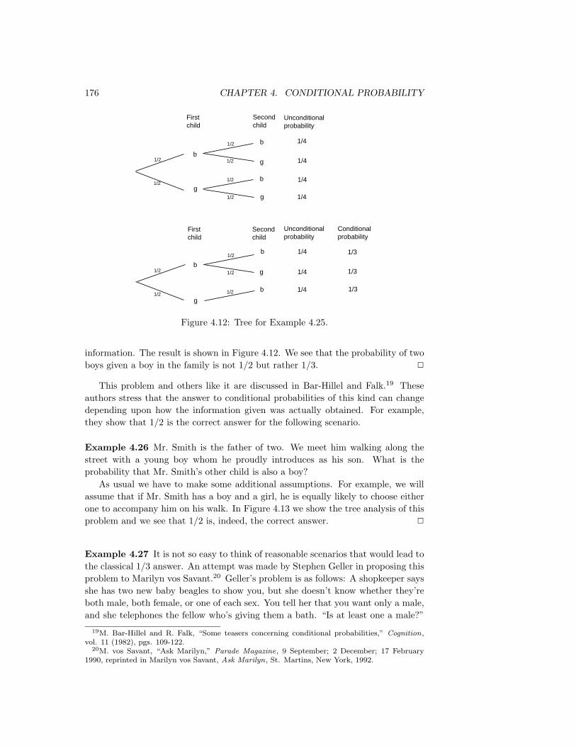
176 CHAPTER 4. CONDITIONAL PROBABILITY
First child
Second child
Conditional probability
First child
Second child
Unconditional probability
b
g
b
g
b
g
b
1/4
1/4
1/4
1/4
1/3
1/3
1/31/4
1/4
1/41/2
1/2
1/2
1/2
1/2
b
g
1/2
1/2
1/2
g
b
Unconditional probability
1/2
1/2
1/2
Figure 4.12: Tree for Example 4.25.
information. The result is shown in Figure 4.12. We see that the probability of twoboys given a boy in the family is not 1/2 but rather 1/3. 2
This problem and others like it are discussed in Bar-Hillel and Falk.19 Theseauthors stress that the answer to conditional probabilities of this kind can changedepending upon how the information given was actually obtained. For example,they show that 1/2 is the correct answer for the following scenario.
Example 4.26 Mr. Smith is the father of two. We meet him walking along thestreet with a young boy whom he proudly introduces as his son. What is theprobability that Mr. Smith’s other child is also a boy?
As usual we have to make some additional assumptions. For example, we willassume that if Mr. Smith has a boy and a girl, he is equally likely to choose eitherone to accompany him on his walk. In Figure 4.13 we show the tree analysis of thisproblem and we see that 1/2 is, indeed, the correct answer. 2
Example 4.27 It is not so easy to think of reasonable scenarios that would lead tothe classical 1/3 answer. An attempt was made by Stephen Geller in proposing thisproblem to Marilyn vos Savant.20 Geller’s problem is as follows: A shopkeeper saysshe has two new baby beagles to show you, but she doesn’t know whether they’reboth male, both female, or one of each sex. You tell her that you want only a male,and she telephones the fellow who’s giving them a bath. “Is at least one a male?”
19M. Bar-Hillel and R. Falk, “Some teasers concerning conditional probabilities,” Cognition,vol. 11 (1982), pgs. 109-122.
20M. vos Savant, “Ask Marilyn,” Parade Magazine, 9 September; 2 December; 17 February1990, reprinted in Marilyn vos Savant, Ask Marilyn, St. Martins, New York, 1992.

4.3. PARADOXES 177
Mr.Smith's children
Walking with Mr.Smith
Unconditional probability
Mr.Smith's children
Walking with Mr. Smith
Unconditional probability
b
bb b
g
g
g
b
1/4
1/8
1/8
1/8
1/8
1/4
1/4
1/4
1/4
1/4
1
1/2
1/2
1/2
1/2
1
bg
gb
gg
b
bb b
b
1/4
1/8
1/8
1/4
1/4
1/4
1
1/2
1/2
bg
gb
Conditional probability
1/2
1/4
1/4
Figure 4.13: Tree for Example 4.26.

178 CHAPTER 4. CONDITIONAL PROBABILITY
she asks. “Yes,” she informs you with a smile. What is the probability that theother one is male?
The reader is asked to decide whether the model which gives an answer of 1/3is a reasonable one to use in this case. 2
In the preceding examples, the apparent paradoxes could easily be resolved byclearly stating the model that is being used and the assumptions that are beingmade. We now turn to some examples in which the paradoxes are not so easilyresolved.
Example 4.28 Two envelopes each contain a certain amount of money. One en-velope is given to Ali and the other to Baba and they are told that one envelopecontains twice as much money as the other. However, neither knows who has thelarger prize. Before anyone has opened their envelope, Ali is asked if she would liketo trade her envelope with Baba. She reasons as follows: Assume that the amountin my envelope is x. If I switch, I will end up with x/2 with probability 1/2, and2x with probability 1/2. If I were given the opportunity to play this game manytimes, and if I were to switch each time, I would, on average, get
12x
2+
12
2x =54x .
This is greater than my average winnings if I didn’t switch.Of course, Baba is presented with the same opportunity and reasons in the same
way to conclude that he too would like to switch. So they switch and each thinksthat his/her net worth just went up by 25%.
Since neither has yet opened any envelope, this process can be repeated and soagain they switch. Now they are back with their original envelopes and yet theythink that their fortune has increased 25% twice. By this reasoning, they couldconvince themselves that by repeatedly switching the envelopes, they could becomearbitrarily wealthy. Clearly, something is wrong with the above reasoning, butwhere is the mistake?
One of the tricks of making paradoxes is to make them slightly more difficult thanis necessary to further befuddle us. As John Finn has suggested, in this paradox wecould just have well started with a simpler problem. Suppose Ali and Baba knowthat I am going to give then either an envelope with $5 or one with $10 and I amgoing to toss a coin to decide which to give to Ali, and then give the other to Baba.Then Ali can argue that Baba has 2x with probability 1/2 and x/2 with probability1/2. This leads Ali to the same conclusion as before. But now it is clear that thisis nonsense, since if Ali has the envelope containing $5, Baba cannot possibly havehalf of this, namely $2.50, since that was not even one of the choices. Similarly, ifAli has $10, Baba cannot have twice as much, namely $20. In fact, in this simplerproblem the possibly outcomes are given by the tree diagram in Figure 4.14. Fromthe diagram, it is clear that neither is made better off by switching. 2
In the above example, Ali’s reasoning is incorrect because he infers that if theamount in his envelope is x, then the probability that his envelope contains the
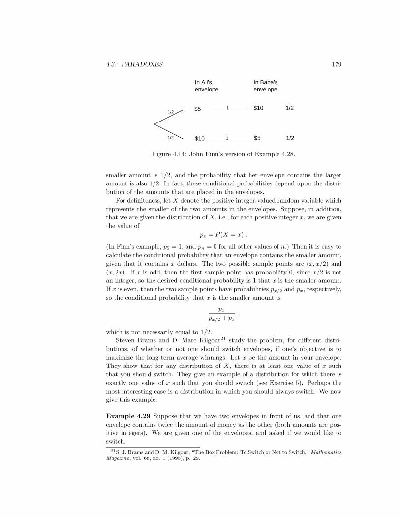
4.3. PARADOXES 179
$5$10
$10$5
1/2
1/21/2
1
11/2
In Ali's envelope
In Baba's envelope
Figure 4.14: John Finn’s version of Example 4.28.
smaller amount is 1/2, and the probability that her envelope contains the largeramount is also 1/2. In fact, these conditional probabilities depend upon the distri-bution of the amounts that are placed in the envelopes.
For definiteness, let X denote the positive integer-valued random variable whichrepresents the smaller of the two amounts in the envelopes. Suppose, in addition,that we are given the distribution of X, i.e., for each positive integer x, we are giventhe value of
px = P (X = x) .
(In Finn’s example, p5 = 1, and pn = 0 for all other values of n.) Then it is easy tocalculate the conditional probability that an envelope contains the smaller amount,given that it contains x dollars. The two possible sample points are (x, x/2) and(x, 2x). If x is odd, then the first sample point has probability 0, since x/2 is notan integer, so the desired conditional probability is 1 that x is the smaller amount.If x is even, then the two sample points have probabilities px/2 and px, respectively,so the conditional probability that x is the smaller amount is
pxpx/2 + px
,
which is not necessarily equal to 1/2.Steven Brams and D. Marc Kilgour21 study the problem, for different distri-
butions, of whether or not one should switch envelopes, if one’s objective is tomaximize the long-term average winnings. Let x be the amount in your envelope.They show that for any distribution of X, there is at least one value of x suchthat you should switch. They give an example of a distribution for which there isexactly one value of x such that you should switch (see Exercise 5). Perhaps themost interesting case is a distribution in which you should always switch. We nowgive this example.
Example 4.29 Suppose that we have two envelopes in front of us, and that oneenvelope contains twice the amount of money as the other (both amounts are pos-itive integers). We are given one of the envelopes, and asked if we would like toswitch.
21S. J. Brams and D. M. Kilgour, “The Box Problem: To Switch or Not to Switch,” MathematicsMagazine, vol. 68, no. 1 (1995), p. 29.

180 CHAPTER 4. CONDITIONAL PROBABILITY
As above, we let X denote the smaller of the two amounts in the envelopes, andlet
px = P (X = x) .
We are now in a position where we can calculate the long-term average winnings, ifwe switch. (This long-term average is an example of a probabilistic concept knownas expectation, and will be discussed in Chapter 6.) Given that one of the twosample points has occurred, the probability that it is the point (x, x/2) is
px/2
px/2 + px,
and the probability that it is the point (x, 2x) is
pxpx/2 + px
.
Thus, if we switch, our long-term average winnings are
px/2
px/2 + px
x
2+
pxpx/2 + px
2x .
If this is greater than x, then it pays in the long run for us to switch. Some routinealgebra shows that the above expression is greater than x if and only if
px/2
px/2 + px<
23. (4.6)
It is interesting to consider whether there is a distribution on the positive integerssuch that the inequality 4.6 is true for all even values of x. Brams and Kilgour22
give the following example.We define px as follows:
px =
13
(23
)k−1
, if x = 2k,0, otherwise.
It is easy to calculate (see Exercise 4) that for all relevant values of x, we have
px/2
px/2 + px=
35,
which means that the inequality 4.6 is always true. 2
So far, we have been able to resolve paradoxes by clearly stating the assumptionsbeing made and by precisely stating the models being used. We end this section bydescribing a paradox which we cannot resolve.
Example 4.30 Suppose that we have two envelopes in front of us, and we aretold that the envelopes contain X and Y dollars, respectively, where X and Y aredifferent positive integers. We randomly choose one of the envelopes, and we open
22ibid.

4.3. PARADOXES 181
it, revealing X, say. Is it possible to determine, with probability greater than 1/2,whether X is the smaller of the two dollar amounts?
Even if we have no knowledge of the joint distribution of X and Y , the surprisinganswer is yes! Here’s how to do it. Toss a fair coin until the first time that headsturns up. Let Z denote the number of tosses required plus 1/2. If Z > X, then wesay that X is the smaller of the two amounts, and if Z < X, then we say that X isthe larger of the two amounts.
First, if Z lies between X and Y , then we are sure to be correct. Since X andY are unequal, Z lies between them with positive probability. Second, if Z is notbetween X and Y , then Z is either greater than both X and Y , or is less than bothX and Y . In either case, X is the smaller of the two amounts with probability 1/2,by symmetry considerations (remember, we chose the envelope at random). Thus,the probability that we are correct is greater than 1/2. 2
Exercises
1 One of the first conditional probability paradoxes was provided by Bertrand.23
It is called the Box Paradox . A cabinet has three drawers. In the first drawerthere are two gold balls, in the second drawer there are two silver balls, andin the third drawer there is one silver and one gold ball. A drawer is picked atrandom and a ball chosen at random from the two balls in the drawer. Giventhat a gold ball was drawn, what is the probability that the drawer with thetwo gold balls was chosen?
2 The following problem is called the two aces problem. This problem, dat-ing back to 1936, has been attributed to the English mathematician J. H.C. Whitehead (see Gridgeman24). This problem was also submitted to Mar-ilyn vos Savant by the master of mathematical puzzles Martin Gardner, whoremarks that it is one of his favorites.
A bridge hand has been dealt, i. e. thirteen cards are dealt to each player.Given that your partner has at least one ace, what is the probability that hehas at least two aces? Given that your partner has the ace of hearts, whatis the probability that he has at least two aces? Answer these questions fora version of bridge in which there are eight cards, namely four aces and fourkings, and each player is dealt two cards. (The reader may wish to solve theproblem with a 52-card deck.)
3 In the preceding exercise, it is natural to ask “How do we get the informationthat the given hand has an ace?” Gridgeman considers two different waysthat we might get this information. (Again, assume the deck consists of eightcards.)
(a) Assume that the person holding the hand is asked to “Name an ace inyour hand” and answers “The ace of hearts.” What is the probabilitythat he has a second ace?
23J. Bertrand, Calcul des Probabilites, Gauthier-Uillars, 1888.24N. T. Gridgeman, Letter, American Statistician, 21 (1967), pgs. 38-39.

182 CHAPTER 4. CONDITIONAL PROBABILITY
(b) Suppose the person holding the hand is asked the more direct question“Do you have the ace of hearts?” and the answer is yes. What is theprobability that he has a second ace?
4 Using the notation introduced in Example 4.29, show that in the example ofBrams and Kilgour, if x is a positive power of 2, then
px/2
px/2 + px=
35.
5 Using the notation introduced in Example 4.29, let
px =
23
(13
)k, if x = 2k,
0, otherwise.
Show that there is exactly one value of x such that if your envelope containsx, then you should switch.
*6 (For bridge players only. From Sutherland.25) Suppose that we are the de-clarer in a hand of bridge, and we have the king, 9, 8, 7, and 2 of a certainsuit, while the dummy has the ace, 10, 5, and 4 of the same suit. Supposethat we want to play this suit in such a way as to maximize the probabilityof having no losers in the suit. We begin by leading the 2 to the ace, and wenote that the queen drops on our left. We then lead the 10 from the dummy,and our right-hand opponent plays the six (after playing the three on the firstround). Should we finesse or play for the drop?
25E. Sutherland, “Restricted Choice — Fact or Fiction?”, Canadian Master Point , November1, 1993.

Chapter 5
Important Distributions andDensities
5.1 Important Distributions
In this chapter, we describe the discrete probability distributions and the continuousprobability densities that occur most often in the analysis of experiments. We willalso show how one simulates these distributions and densities on a computer.
Discrete Uniform Distribution
In Chapter 1, we saw that in many cases, we assume that all outcomes of an exper-iment are equally likely. If X is a random variable which represents the outcomeof an experiment of this type, then we say that X is uniformly distributed. If thesample space S is of size n, where 0 < n <∞, then the distribution function m(ω)is defined to be 1/n for all ω ∈ S. As is the case with all of the discrete probabil-ity distributions discussed in this chapter, this experiment can be simulated on acomputer using the program GeneralSimulation. However, in this case, a fasteralgorithm can be used instead. (This algorithm was described in Chapter 1; werepeat the description here for completeness.) The expression
1 + bn (rnd)c
takes on as a value each integer between 1 and n with probability 1/n (the notationbxc denotes the greatest integer not exceeding x). Thus, if the possible outcomesof the experiment are labelled ω1 ω2, . . . , ωn, then we use the above expression torepresent the subscript of the output of the experiment.
If the sample space is a countably infinite set, such as the set of positive integers,then it is not possible to have an experiment which is uniform on this set (seeExercise 3). If the sample space is an uncountable set, with positive, finite length,such as the interval [0, 1], then we use continuous density functions (see Section 5.2).
183
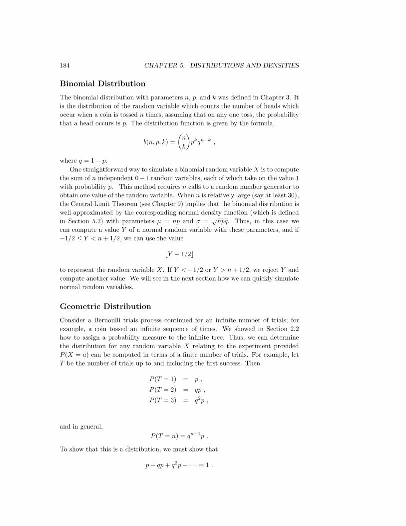
184 CHAPTER 5. DISTRIBUTIONS AND DENSITIES
Binomial Distribution
The binomial distribution with parameters n, p, and k was defined in Chapter 3. Itis the distribution of the random variable which counts the number of heads whichoccur when a coin is tossed n times, assuming that on any one toss, the probabilitythat a head occurs is p. The distribution function is given by the formula
b(n, p, k) =(n
k
)pkqn−k ,
where q = 1− p.One straightforward way to simulate a binomial random variableX is to compute
the sum of n independent 0−1 random variables, each of which take on the value 1with probability p. This method requires n calls to a random number generator toobtain one value of the random variable. When n is relatively large (say at least 30),the Central Limit Theorem (see Chapter 9) implies that the binomial distribution iswell-approximated by the corresponding normal density function (which is definedin Section 5.2) with parameters µ = np and σ =
√npq. Thus, in this case we
can compute a value Y of a normal random variable with these parameters, and if−1/2 ≤ Y < n+ 1/2, we can use the value
bY + 1/2c
to represent the random variable X. If Y < −1/2 or Y > n+ 1/2, we reject Y andcompute another value. We will see in the next section how we can quickly simulatenormal random variables.
Geometric Distribution
Consider a Bernoulli trials process continued for an infinite number of trials; forexample, a coin tossed an infinite sequence of times. We showed in Section 2.2how to assign a probability measure to the infinite tree. Thus, we can determinethe distribution for any random variable X relating to the experiment providedP (X = a) can be computed in terms of a finite number of trials. For example, letT be the number of trials up to and including the first success. Then
P (T = 1) = p ,
P (T = 2) = qp ,
P (T = 3) = q2p ,
and in general,P (T = n) = qn−1p .
To show that this is a distribution, we must show that
p+ qp+ q2p+ · · · = 1 .
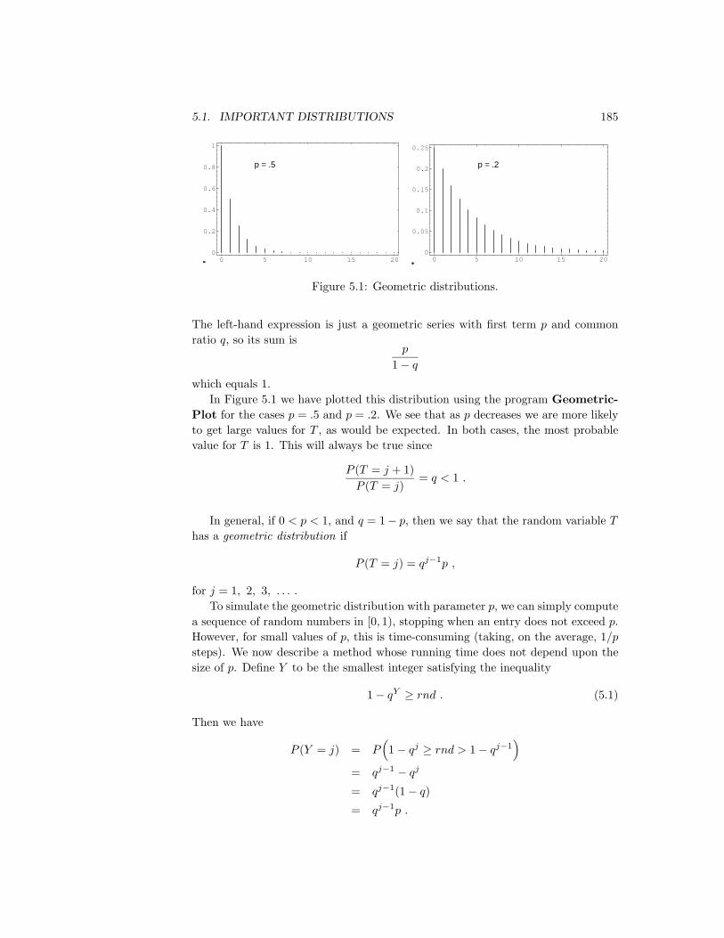
5.1. IMPORTANT DISTRIBUTIONS 185
0 5 10 15 200
0.2
0.4
0.6
0.8
1
p = .5
0 5 10 15 200
0.05
0.1
0.15
0.2
0.25
p = .2
Figure 5.1: Geometric distributions.
The left-hand expression is just a geometric series with first term p and commonratio q, so its sum is
p
1− qwhich equals 1.
In Figure 5.1 we have plotted this distribution using the program Geometric-Plot for the cases p = .5 and p = .2. We see that as p decreases we are more likelyto get large values for T , as would be expected. In both cases, the most probablevalue for T is 1. This will always be true since
P (T = j + 1)P (T = j)
= q < 1 .
In general, if 0 < p < 1, and q = 1− p, then we say that the random variable Thas a geometric distribution if
P (T = j) = qj−1p ,
for j = 1, 2, 3, . . . .To simulate the geometric distribution with parameter p, we can simply compute
a sequence of random numbers in [0, 1), stopping when an entry does not exceed p.However, for small values of p, this is time-consuming (taking, on the average, 1/psteps). We now describe a method whose running time does not depend upon thesize of p. Define Y to be the smallest integer satisfying the inequality
1− qY ≥ rnd . (5.1)
Then we have
P (Y = j) = P(
1− qj ≥ rnd > 1− qj−1)
= qj−1 − qj
= qj−1(1− q)= qj−1p .

186 CHAPTER 5. DISTRIBUTIONS AND DENSITIES
Thus, Y is geometrically distributed with parameter p. To generate Y , all we haveto do is solve Equation 5.1 for Y . We obtain
Y =
⌈log(1− rnd)
log q
⌉,
where the notation dxe means the least integer which is greater than or equal to x.Since log(1− rnd) and log(rnd) are identically distributed, Y can also be generatedusing the equation
Y =
⌈log rnd
log q
⌉.
Example 5.1 The geometric distribution plays an important role in the theory ofqueues, or waiting lines. For example, suppose a line of customers waits for serviceat a counter. It is often assumed that, in each small time unit, either 0 or 1 newcustomers arrive at the counter. The probability that a customer arrives is p andthat no customer arrives is q = 1 − p. Then the time T until the next arrival hasa geometric distribution. It is natural to ask for the probability that no customerarrives in the next k time units, that is, for P (T > k). This is given by
P (T > k) =∞∑
j=k+1
qj−1p = qk(p+ qp+ q2p+ · · ·)
= qk .
This probability can also be found by noting that we are asking for no successes(i.e., arrivals) in a sequence of k consecutive time units, where the probability of asuccess in any one time unit is p. Thus, the probability is just qk, since arrivals inany two time units are independent events.
It is often assumed that the length of time required to service a customer alsohas a geometric distribution but with a different value for p. This implies a ratherspecial property of the service time. To see this, let us compute the conditionalprobability
P (T > r + s |T > r) =P (T > r + s)P (T > r)
=qr+s
qr= qs .
Thus, the probability that the customer’s service takes s more time units is inde-pendent of the length of time r that the customer has already been served. Becauseof this interpretation, this property is called the “memoryless” property, and is alsoobeyed by the exponential distribution. (Fortunately, not too many service stationshave this property.) 2
Negative Binomial Distribution
Suppose we are given a coin which has probability p of coming up heads when it istossed. We fix a positive integer k, and toss the coin until the kth head appears. We

5.1. IMPORTANT DISTRIBUTIONS 187
let X represent the number of tosses. When k = 1, X is geometrically distributed.For a general k, we say that X has a negative binomial distribution. We nowcalculate the probability distribution of X. If X = x, then it must be true thatthere were exactly k − 1 heads thrown in the first x − 1 tosses, and a head musthave been thrown on the xth toss. There are(
x− 1k − 1
)sequences of length x with these properties, and each of them is assigned the sameprobability, namely
pk−1qx−k .
Therefore, if we defineu(x, k, p) = P (X = x) ,
then
u(x, k, p) =(x− 1k − 1
)pkqx−k .
One can simulate this on a computer by simulating the tossing of a coin. Thefollowing algorithm is, in general, much faster. We note that X can be understoodas the sum of k outcomes of a geometrically distributed experiment with parameterp. Thus, we can use the following sum as a means of generating X:
k∑j=1
⌈log rndj
log q
⌉.
Example 5.2 A fair coin is tossed until the second time a head turns up. Thedistribution for the number of tosses is u(x, 2, p). Thus the probability that x tossesare needed to obtain two heads is found by letting k = 2 in the above formula. Weobtain
u(x, 2, 1/2) =(x− 1
1
)12x
,
for x = 2, 3, . . . .In Figure 5.2 we give a graph of the distribution for k = 2 and p = .25. Note
that the distribution is quite asymmetric, with a long tail reflecting the fact thatlarge values of x are possible. 2
Poisson Distribution
The Poisson distribution arises in many situations. It is safe to say that it is one ofthe three most important discrete probability distributions (the other two being theuniform and the binomial distributions). The Poisson distribution can be viewedas arising from the binomial distribution or from the exponential density. We shallnow explain its connection with the former; its connection with the latter will beexplained in the next section.

188 CHAPTER 5. DISTRIBUTIONS AND DENSITIES
5 10 15 20 25 300
0.02
0.04
0.06
0.08
0.1
Figure 5.2: Negative binomial distribution with k = 2 and p = .25.
Suppose that we have a situation in which a certain kind of occurrence happensat random over a period of time. For example, the occurrences that we are interestedin might be incoming telephone calls to a police station in a large city. We wantto model this situation so that we can consider the probabilities of events suchas more than 10 phone calls occurring in a 5-minute time interval. Presumably,in our example, there would be more incoming calls between 6:00 and 7:00 P.M.
than between 4:00 and 5:00 A.M., and this fact would certainly affect the aboveprobability. Thus, to have a hope of computing such probabilities, we must assumethat the average rate, i.e., the average number of occurrences per minute, is aconstant. This rate we will denote by λ. (Thus, in a given 5-minute time interval,we would expect about 5λ occurrences.) This means that if we were to apply ourmodel to the two time periods given above, we would simply use different ratesfor the two time periods, thereby obtaining two different probabilities for the givenevent.
Our next assumption is that the number of occurrences in two non-overlappingtime intervals are independent. In our example, this means that the events thatthere are j calls between 5:00 and 5:15 P.M. and k calls between 6:00 and 6:15 P.M.
on the same day are independent.
We can use the binomial distribution to model this situation. We imagine thata given time interval is broken up into n subintervals of equal length. If the subin-tervals are sufficiently short, we can assume that two or more occurrences happenin one subinterval with a probability which is negligible in comparison with theprobability of at most one occurrence. Thus, in each subinterval, we are assumingthat there is either 0 or 1 occurrence. This means that the sequence of subintervalscan be thought of as a sequence of Bernoulli trials, with a success corresponding toan occurrence in the subinterval.

5.1. IMPORTANT DISTRIBUTIONS 189
To decide upon the proper value of p, the probability of an occurrence in a givensubinterval, we reason as follows. On the average, there are λt occurrences in atime interval of length t. If this time interval is divided into n subintervals, thenwe would expect, using the Bernoulli trials interpretation, that there should be npoccurrences. Thus, we want
λt = np ,
sop =
λt
n.
We now wish to consider the random variable X, which counts the number ofoccurrences in a given time interval. We want to calculate the distribution of X.For ease of calculation, we will assume that the time interval is of length 1; for timeintervals of arbitrary length t, see Exercise 11. We know that
P (X = 0) = b(n, p, 0) = (1− p)n =(
1− λ
n
)n.
For large n, this is approximately e−λ. It is easy to calculate that for any fixed k,we have
b(n, p, k)b(n, p, k − 1)
=λ− (k − 1)p
kq
which, for large n (and therefore small p) is approximately λ/k. Thus, we have
P (X = 1) ≈ λe−λ ,
and in general,
P (X = k) ≈ λk
k!e−λ . (5.2)
The above distribution is the Poisson distribution. We note that it must be checkedthat the distribution given in Equation 5.2 really is a distribution, i.e., that itsvalues are non-negative and sum to 1. (See Exercise 12.)
The Poisson distribution is used as an approximation to the binomial distribu-tion when the parameters n and p are large and small, respectively (see Examples 5.3and 5.4). However, the Poisson distribution also arises in situations where it maynot be easy to interpret or measure the parameters n and p (see Example 5.5).
Example 5.3 A typesetter makes, on the average, one mistake per 1000 words.Assume that he is setting a book with 100 words to a page. Let S100 be the numberof mistakes that he makes on a single page. Then the exact probability distributionfor S100 would be obtained by considering S100 as a result of 100 Bernoulli trialswith p = 1/1000. The expected value of S100 is λ = 100(1/1000) = .1. The exactprobability that S100 = j is b(100, 1/1000, j), and the Poisson approximation is
e−.1(.1)j
j!.
In Table 5.1 we give, for various values of n and p, the exact values computed bythe binomial distribution and the Poisson approximation. 2

190 CHAPTER 5. DISTRIBUTIONS AND DENSITIES
Poisson Binomial Poisson Binomial Poisson Binomialn = 100 n = 100 n = 1000
j λ = .1 p = .001 λ = 1 p = .01 λ = 10 p = .010 .9048 .9048 .3679 .3660 .0000 .00001 .0905 .0905 .3679 .3697 .0005 .00042 .0045 .0045 .1839 .1849 .0023 .00223 .0002 .0002 .0613 .0610 .0076 .00744 .0000 .0000 .0153 .0149 .0189 .01865 .0031 .0029 .0378 .03746 .0005 .0005 .0631 .06277 .0001 .0001 .0901 .09008 .0000 .0000 .1126 .11289 .1251 .125610 .1251 .125711 .1137 .114312 .0948 .095213 .0729 .073114 .0521 .052015 .0347 .034516 .0217 .021517 .0128 .012618 .0071 .006919 .0037 .003620 .0019 .001821 .0009 .000922 .0004 .000423 .0002 .000224 .0001 .000125 .0000 .0000
Table 5.1: Poisson approximation to the binomial distribution.

5.1. IMPORTANT DISTRIBUTIONS 191
Example 5.4 In his book,1 Feller discusses the statistics of flying bomb hits in thesouth of London during the Second World War.
Assume that you live in a district of size 10 blocks by 10 blocks so that the totaldistrict is divided into 100 small squares. How likely is it that the square in whichyou live will receive no hits if the total area is hit by 400 bombs?
We assume that a particular bomb will hit your square with probability 1/100.Since there are 400 bombs, we can regard the number of hits that your squarereceives as the number of successes in a Bernoulli trials process with n = 400 andp = 1/100. Thus we can use the Poisson distribution with λ = 400 · 1/100 = 4 toapproximate the probability that your square will receive j hits. This probabilityis p(j) = e−44j/j!. The expected number of squares that receive exactly j hitsis then 100 · p(j). It is easy to write a program LondonBombs to simulate thissituation and compare the expected number of squares with j hits with the observednumber. In Exercise 26 you are asked to compare the actual observed data withthat predicted by the Poisson distribution.
In Figure 5.3, we have shown the simulated hits, together with a spike graphshowing both the observed and predicted frequencies. The observed frequencies areshown as squares, and the predicted frequencies are shown as dots. 2
If the reader would rather not consider flying bombs, he is invited to instead consideran analogous situation involving cookies and raisins. We assume that we have madeenough cookie dough for 500 cookies. We put 600 raisins in the dough, and mix itthoroughly. One way to look at this situation is that we have 500 cookies, and afterplacing the cookies in a grid on the table, we throw 600 raisins at the cookies. (SeeExercise 22.)
Example 5.5 Suppose that in a certain fixed amount A of blood, the averagehuman has 40 white blood cells. Let X be the random variable which gives thenumber of white blood cells in a random sample of size A from a random individual.We can think of X as binomially distributed with each white blood cell in the bodyrepresenting a trial. If a given white blood cell turns up in the sample, then thetrial corresponding to that blood cell was a success. Then p should be taken asthe ratio of A to the total amount of blood in the individual, and n will be thenumber of white blood cells in the individual. Of course, in practice, neither ofthese parameters is very easy to measure accurately, but presumably the number40 is easy to measure. But for the average human, we then have 40 = np, so wecan think of X as being Poisson distributed, with parameter λ = 40. In this case,it is easier to model the situation using the Poisson distribution than the binomialdistribution. 2
To simulate a Poisson random variable on a computer, a good way is to takeadvantage of the relationship between the Poisson distribution and the exponentialdensity. This relationship and the resulting simulation algorithm will be describedin the next section.
1ibid., p. 161.

192 CHAPTER 5. DISTRIBUTIONS AND DENSITIES
0 2 4 6 8 10
0
0.05
0.1
0.15
0.2
Figure 5.3: Flying bomb hits.

5.1. IMPORTANT DISTRIBUTIONS 193
Hypergeometric Distribution
Suppose that we have a set of N balls, of which k are red and N − k are blue. Wechoose n of these balls, without replacement, and define X to be the number of redballs in our sample. The distribution of X is called the hypergeometric distribution.We note that this distribution depends upon three parameters, namely N , k, andn. There does not seem to be a standard notation for this distribution; we will usethe notation h(N, k, n, x) to denote P (X = x). This probability can be found bynoting that there are (
N
n
)different samples of size n, and the number of such samples with exactly x red ballsis obtained by multiplying the number of ways of choosing x red balls from the setof k red balls and the number of ways of choosing n− x blue balls from the set ofN − k blue balls. Hence, we have
h(N, k, n, x) =
(kx
)(N−kn−x
)(Nn
) .
This distribution can be generalized to the case where there are more than twotypes of objects. (See Exercise 40.)
If we let N and k tend to∞, in such a way that the ratio k/N remains fixed, thenthe hypergeometric distribution tends to the binomial distribution with parametersn and p = k/N . This is reasonable because if N and k are much larger than n, thenwhether we choose our sample with or without replacement should not affect theprobabilities very much, and the experiment consisting of choosing with replacementyields a binomially distributed random variable (see Exercise 44).
An example of how this distribution might be used is given in Exercises 36 and37. We now give another example involving the hypergeometric distribution. Itillustrates a statistical test called Fisher’s Exact Test.
Example 5.6 It is often of interest to consider two traits, such as eye color andhair color, and to ask whether there is an association between the two traits. Twotraits are associated if knowing the value of one of the traits for a given personallows us to predict the value of the other trait for that person. The stronger theassociation, the more accurate the predictions become. If there is no associationbetween the traits, then we say that the traits are independent. In this example, wewill use the traits of gender and political party, and we will assume that there areonly two possible genders, female and male, and only two possible political parties,Democratic and Republican.
Suppose that we have collected data concerning these traits. To test whetherthere is an association between the traits, we first assume that there is no associationbetween the two traits. This gives rise to an “expected” data set, in which knowledgeof the value of one trait is of no help in predicting the value of the other trait. Ourcollected data set usually differs from this expected data set. If it differs by quite abit, then we would tend to reject the assumption of independence of the traits. To

194 CHAPTER 5. DISTRIBUTIONS AND DENSITIES
Democrat RepublicanFemale 24 4 28Male 8 14 22
32 18 50
Table 5.2: Observed data.
Democrat RepublicanFemale s11 s12 t11
Male s21 s22 t12
t21 t22 n
Table 5.3: General data table.
nail down what is meant by “quite a bit,” we decide which possible data sets differfrom the expected data set by at least as much as ours does, and then we computethe probability that any of these data sets would occur under the assumption ofindependence of traits. If this probability is small, then it is unlikely that thedifference between our collected data set and the expected data set is due entirelyto chance.
Suppose that we have collected the data shown in Table 5.2. The row and columnsums are called marginal totals, or marginals. In what follows, we will denote therow sums by t11 and t12, and the column sums by t21 and t22. The ijth entry inthe table will be denoted by sij . Finally, the size of the data set will be denotedby n. Thus, a general data table will look as shown in Table 5.3. We now explainthe model which will be used to construct the “expected” data set. In the model,we assume that the two traits are independent. We then put t21 yellow balls andt22 green balls, corresponding to the Democratic and Republican marginals, intoan urn. We draw t11 balls, without replacement, from the urn, and call these ballsfemales. The t12 balls remaining in the urn are called males. In the specific caseunder consideration, the probability of getting the actual data under this model isgiven by the expression (
3224
)(184
)(5028
) ,
i.e., a value of the hypergeometric distribution.We are now ready to construct the expected data set. If we choose 28 balls
out of 50, we should expect to see, on the average, the same percentage of yellowballs in our sample as in the urn. Thus, we should expect to see, on the average,28(32/50) = 17.92 ≈ 18 yellow balls in our sample. (See Exercise 36.) The otherexpected values are computed in exactly the same way. Thus, the expected dataset is shown in Table 5.4. We note that the value of s11 determines the otherthree values in the table, since the marginals are all fixed. Thus, in consideringthe possible data sets that could appear in this model, it is enough to consider thevarious possible values of s11. In the specific case at hand, what is the probability

5.1. IMPORTANT DISTRIBUTIONS 195
Democrat RepublicanFemale 18 10 28Male 14 8 22
32 18 50
Table 5.4: Expected data.
of drawing exactly a yellow balls, i.e., what is the probability that s11 = a? It is(32a
)(18
28−a)(
5028
) . (5.3)
We are now ready to decide whether our actual data differs from the expecteddata set by an amount which is greater than could be reasonably attributed tochance alone. We note that the expected number of female Democrats is 18, butthe actual number in our data is 24. The other data sets which differ from theexpected data set by more than ours correspond to those where the number offemale Democrats equals 25, 26, 27, or 28. Thus, to obtain the required probability,we sum the expression in (5.3) from a = 24 to a = 28. We obtain a value of .000395.Thus, we should reject the hypothesis that the two traits are independent. 2
Finally, we turn to the question of how to simulate a hypergeometric randomvariable X. Let us assume that the parameters for X are N , k, and n. We imaginethat we have a set of N balls, labelled from 1 to N . We decree that the first k ofthese balls are red, and the rest are blue. Suppose that we have chosen m balls,and that j of them are red. Then there are k − j red balls left, and N −m ballsleft. Thus, our next choice will be red with probability
k − jN −m .
So at this stage, we choose a random number in [0, 1], and report that a red ball hasbeen chosen if and only if the random number does not exceed the above expression.Then we update the values of m and j, and continue until n balls have been chosen.
Benford Distribution
Our next example of a distribution comes from the study of leading digits in datasets. It turns out that many data sets that occur “in real life” have the property thatthe first digits of the data are not uniformly distributed over the set 1, 2, . . . , 9.Rather, it appears that the digit 1 is most likely to occur, and that the distributionis monotonically decreasing on the set of possible digits. The Benford distributionappears, in many cases, to fit such data. Many explanations have been given for theoccurrence of this distribution. Possibly the most convincing explanation is thatthis distribution is the only one that is invariant under a change of scale. If onethinks of certain data sets as somehow “naturally occurring,” then the distributionshould be unaffected by which units are chosen in which to represent the data, i.e.,the distribution should be invariant under change of scale.
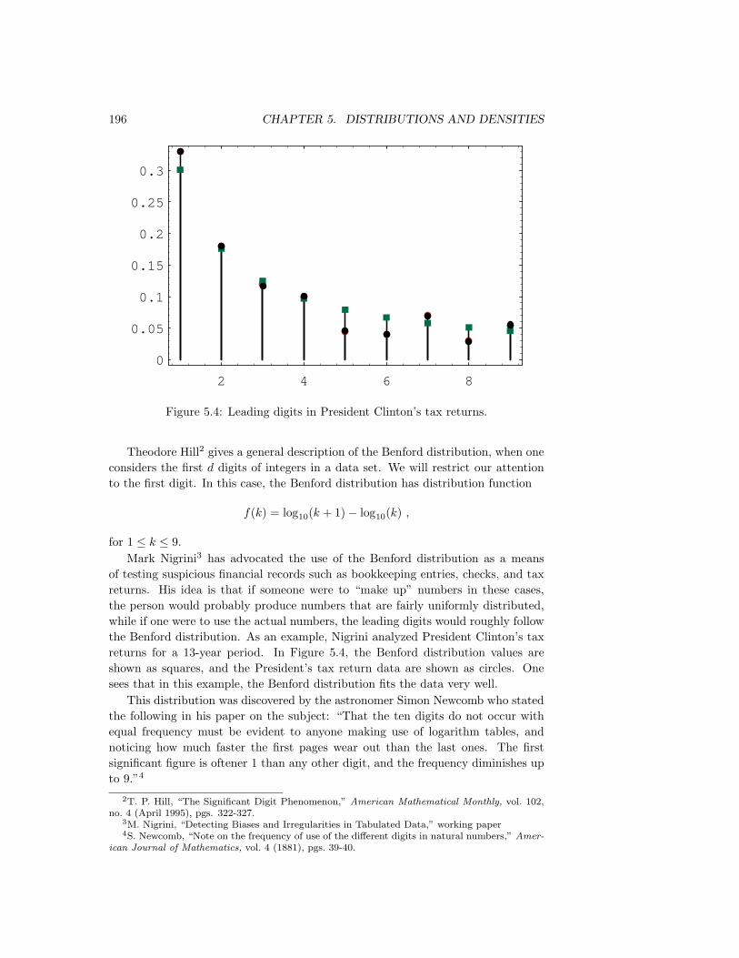
196 CHAPTER 5. DISTRIBUTIONS AND DENSITIES
2 4 6 8
0
0.05
0.1
0.15
0.2
0.25
0.3
Figure 5.4: Leading digits in President Clinton’s tax returns.
Theodore Hill2 gives a general description of the Benford distribution, when oneconsiders the first d digits of integers in a data set. We will restrict our attentionto the first digit. In this case, the Benford distribution has distribution function
f(k) = log10(k + 1)− log10(k) ,
for 1 ≤ k ≤ 9.Mark Nigrini3 has advocated the use of the Benford distribution as a means
of testing suspicious financial records such as bookkeeping entries, checks, and taxreturns. His idea is that if someone were to “make up” numbers in these cases,the person would probably produce numbers that are fairly uniformly distributed,while if one were to use the actual numbers, the leading digits would roughly followthe Benford distribution. As an example, Nigrini analyzed President Clinton’s taxreturns for a 13-year period. In Figure 5.4, the Benford distribution values areshown as squares, and the President’s tax return data are shown as circles. Onesees that in this example, the Benford distribution fits the data very well.
This distribution was discovered by the astronomer Simon Newcomb who statedthe following in his paper on the subject: “That the ten digits do not occur withequal frequency must be evident to anyone making use of logarithm tables, andnoticing how much faster the first pages wear out than the last ones. The firstsignificant figure is oftener 1 than any other digit, and the frequency diminishes upto 9.”4
2T. P. Hill, “The Significant Digit Phenomenon,” American Mathematical Monthly, vol. 102,no. 4 (April 1995), pgs. 322-327.
3M. Nigrini, “Detecting Biases and Irregularities in Tabulated Data,” working paper4S. Newcomb, “Note on the frequency of use of the different digits in natural numbers,” Amer-
ican Journal of Mathematics, vol. 4 (1881), pgs. 39-40.

5.1. IMPORTANT DISTRIBUTIONS 197
Exercises
1 For which of the following random variables would it be appropriate to assigna uniform distribution?
(a) Let X represent the roll of one die.
(b) Let X represent the number of heads obtained in three tosses of a coin.
(c) A roulette wheel has 38 possible outcomes: 0, 00, and 1 through 36. LetX represent the outcome when a roulette wheel is spun.
(d) Let X represent the birthday of a randomly chosen person.
(e) Let X represent the number of tosses of a coin necessary to achieve ahead for the first time.
2 Let n be a positive integer. Let S be the set of integers between 1 andn. Consider the following process: We remove a number from S and writeit down. We repeat this until S is empty. The result is a permutation ofthe integers from 1 to n. Let X denote this permutation. Is X uniformlydistributed?
3 Let X be a random variable which can take on countably many values. Showthat X cannot be uniformly distributed.
4 Suppose we are attending a college which has 3000 students. We wish tochoose a subset of size 100 from the student body. Let X represent the subset,chosen using the following possible strategies. For which strategies would itbe appropriate to assign the uniform distribution to X? If it is appropriate,what probability should we assign to each outcome?
(a) Take the first 100 students who enter the cafeteria to eat lunch.
(b) Ask the Registrar to sort the students by their Social Security number,and then take the first 100 in the resulting list.
(c) Ask the Registrar for a set of cards, with each card containing the nameof exactly one student, and with each student appearing on exactly onecard. Throw the cards out of a third-story window, then walk outsideand pick up the first 100 cards that you find.
5 Under the same conditions as in the preceding exercise, can you describea procedure which, if used, would produce each possible outcome with thesame probability? Can you describe such a procedure that does not rely on acomputer or a calculator?
6 Let X1, X2, . . . , Xn be n mutually independent random variables, each ofwhich is uniformly distributed on the integers from 1 to k. Let Y denote theminimum of the Xi’s. Find the distribution of Y .
7 A die is rolled until the first time T that a six turns up.
(a) What is the probability distribution for T?

198 CHAPTER 5. DISTRIBUTIONS AND DENSITIES
(b) Find P (T > 3).
(c) Find P (T > 6|T > 3).
8 If a coin is tossed a sequence of times, what is the probability that the firsthead will occur after the fifth toss, given that it has not occurred in the firsttwo tosses?
9 A worker for the Department of Fish and Game is assigned the job of esti-mating the number of trout in a certain lake of modest size. She proceeds asfollows: She catches 100 trout, tags each of them, and puts them back in thelake. One month later, she catches 100 more trout, and notes that 10 of themhave tags.
(a) Without doing any fancy calculations, give a rough estimate of the num-ber of trout in the lake.
(b) Let N be the number of trout in the lake. Find an expression, in termsof N , for the probability that the worker would catch 10 tagged troutout of the 100 trout that she caught the second time.
(c) Find the value of N which maximizes the expression in part (b). Thisvalue is called the maximum likelihood estimate for the unknown quantityN . Hint : Consider the ratio of the expressions for successive values ofN .
10 A census in the United States is an attempt to count everyone in the country.It is inevitable that many people are not counted. The U. S. Census Bureauproposed a way to estimate the number of people who were not counted bythe latest census. Their proposal was as follows: In a given locality, let Ndenote the actual number of people who live there. Assume that the censuscounted n1 people living in this area. Now, another census was taken in thelocality, and n2 people were counted. In addition, n12 people were countedboth times.
(a) Given N , n1, and n2, let X denote the number of people counted bothtimes. Find the probability that X = k, where k is a fixed positiveinteger between 0 and n2.
(b) Now assume that X = n12. Find the value of N which maximizes theexpression in part (a). Hint : Consider the ratio of the expressions forsuccessive values of N .
11 Suppose that X is a random variable which represents the number of callscoming in to a police station in a one-minute interval. In the text, we showedthat X could be modelled using a Poisson distribution with parameter λ,where this parameter represents the average number of incoming calls perminute. Now suppose that Y is a random variable which represents the num-ber of incoming calls in an interval of length t. Show that the distribution ofY is given by
P (Y = k) = e−λt(λt)k
k!,

5.1. IMPORTANT DISTRIBUTIONS 199
i.e., Y is Poisson with parameter λt. Hint : Suppose a Martian were to observethe police station. Let us also assume that the basic time interval used onMars is exactly t Earth minutes. Finally, we will assume that the Martianunderstands the derivation of the Poisson distribution in the text. Whatwould she write down for the distribution of Y ?
12 Show that the values of the Poisson distribution given in Equation 5.2 sum to1.
13 The Poisson distribution with parameter λ = .3 has been assigned for theoutcome of an experiment. Let X be the outcome function. Find P (X = 0),P (X = 1), and P (X > 1).
14 On the average, only 1 person in 1000 has a particular rare blood type.
(a) Find the probability that, in a city of 10,000 people, no one has thisblood type.
(b) How many people would have to be tested to give a probability greaterthan 1/2 of finding at least one person with this blood type?
15 Write a program for the user to input n, p, j and have the program print outthe exact value of b(n, p, k) and the Poisson approximation to this value.
16 Assume that, during each second, a Dartmouth switchboard receives one callwith probability .01 and no calls with probability .99. Use the Poisson ap-proximation to estimate the probability that the operator will miss at mostone call if she takes a 5-minute coffee break.
17 The probability of a royal flush in a poker hand is p = 1/649,740. How largemust n be to render the probability of having no royal flush in n hands smallerthan 1/e?
18 A baker blends 600 raisins and 400 chocolate chips into a dough mix and,from this, makes 500 cookies.
(a) Find the probability that a randomly picked cookie will have no raisins.
(b) Find the probability that a randomly picked cookie will have exactly twochocolate chips.
(c) Find the probability that a randomly chosen cookie will have at leasttwo bits (raisins or chips) in it.
19 The probability that, in a bridge deal, one of the four hands has all heartsis approximately 6.3 × 10⁻¹². In a city with about 50,000 bridge players theresident probability expert is called on the average once a year (usually late atnight) and told that the caller has just been dealt a hand of all hearts. Shouldshe suspect that some of these callers are the victims of practical jokes?
200 CHAPTER 5. DISTRIBUTIONS AND DENSITIES
20 An advertiser drops 10,000 leaflets on a city which has 2000 blocks. Assumethat each leaflet has an equal chance of landing on each block. What is theprobability that a particular block will receive no leaflets?
21 In a class of 80 students, the professor calls on 1 student chosen at randomfor a recitation in each class period. There are 32 class periods in a term.
(a) Write a formula for the exact probability that a given student is calledupon j times during the term.
(b) Write a formula for the Poisson approximation for this probability. Usingyour formula estimate the probability that a given student is called uponmore than twice.
22 Assume that we are making raisin cookies. We put a box of 600 raisins intoour dough mix, mix up the dough, then make from the dough 500 cookies.We then ask for the probability that a randomly chosen cookie will have0, 1, 2, . . . raisins. Consider the cookies as trials in an experiment, andlet X be the random variable which gives the number of raisins in a givencookie. Then we can regard the number of raisins in a cookie as the resultof n = 600 independent trials with probability p = 1/500 for success on eachtrial. Since n is large and p is small, we can use the Poisson approximationwith λ = 600(1/500) = 1.2. Determine the probability that a given cookiewill have at least five raisins.
23 For a certain experiment, the Poisson distribution with parameter λ = m hasbeen assigned. Show that a most probable outcome for the experiment isthe integer value k such that m − 1 ≤ k ≤ m. Under what conditions willthere be two most probable values? Hint : Consider the ratio of successiveprobabilities.
24 When John Kemeny was chair of the Mathematics Department at DartmouthCollege, he received an average of ten letters each day. On a certain weekdayhe received no mail and wondered if it was a holiday. To decide this hecomputed the probability that, in ten years, he would have at least 1 daywithout any mail. He assumed that the number of letters he received on agiven day has a Poisson distribution. What probability did he find? Hint :Apply the Poisson distribution twice. First, to find the probability that, in3000 days, he will have at least 1 day without mail, assuming each year hasabout 300 days on which mail is delivered.
25 Reese Prosser never puts money in a 10-cent parking meter in Hanover. Heassumes that there is a probability of .05 that he will be caught. The firstoffense costs nothing, the second costs 2 dollars, and subsequent offenses cost5 dollars each. Under his assumptions, how does the expected cost of parking100 times without paying the meter compare with the cost of paying the metereach time?

5.1. IMPORTANT DISTRIBUTIONS 201
Number of deaths Number of corps with x deaths in a given year0 1441 912 323 114 2
Table 5.5: Mule kicks.
26 Feller5 discusses the statistics of flying bomb hits in an area in the south ofLondon during the Second World War. The area in question was divided into24 × 24 = 576 small areas. The total number of hits was 537. There were229 squares with 0 hits, 211 with 1 hit, 93 with 2 hits, 35 with 3 hits, 7 with4 hits, and 1 with 5 or more. Assuming the hits were purely random, use thePoisson approximation to find the probability that a particular square wouldhave exactly k hits. Compute the expected number of squares that wouldhave 0, 1, 2, 3, 4, and 5 or more hits and compare this with the observedresults.
27 Assume that the probability that there is a significant accident in a nuclearpower plant during one year’s time is .001. If a country has 100 nuclear plants,estimate the probability that there is at least one such accident during a givenyear.
28 An airline finds that 4 percent of the passengers that make reservations ona particular flight will not show up. Consequently, their policy is to sell 100reserved seats on a plane that has only 98 seats. Find the probability thatevery person who shows up for the flight will find a seat available.
29 The king’s coinmaster boxes his coins 500 to a box and puts 1 counterfeit coinin each box. The king is suspicious, but, instead of testing all the coins in1 box, he tests 1 coin chosen at random out of each of 500 boxes. What is theprobability that he finds at least one fake? What is it if the king tests 2 coinsfrom each of 250 boxes?
30 (From Kemeny6) Show that, if you make 100 bets on the number 17 atroulette at Monte Carlo (see Example 6.13), you will have a probability greaterthan 1/2 of coming out ahead. What is your expected winning?
31 In one of the first studies of the Poisson distribution, von Bortkiewicz7 con-sidered the frequency of deaths from kicks in the Prussian army corps. Fromthe study of 14 corps over a 20-year period, he obtained the data shown inTable 5.5. Fit a Poisson distribution to this data and see if you think thatthe Poisson distribution is appropriate.
5ibid., p. 161.6Private communication.7L. von Bortkiewicz, Das Gesetz der Kleinen Zahlen (Leipzig: Teubner, 1898), p. 24.

202 CHAPTER 5. DISTRIBUTIONS AND DENSITIES
32 It is often assumed that the auto traffic that arrives at the intersection duringa unit time period has a Poisson distribution with expected value m. Assumethat the number of cars X that arrive at an intersection from the north in unittime has a Poisson distribution with parameter λ = m and the number Y thatarrive from the west in unit time has a Poisson distribution with parameterλ = m. If X and Y are independent, show that the total number X + Y
that arrive at the intersection in unit time has a Poisson distribution withparameter λ = m+ m.
33 Cars coming along Magnolia Street come to a fork in the road and have tochoose either Willow Street or Main Street to continue. Assume that thenumber of cars that arrive at the fork in unit time has a Poisson distributionwith parameter λ = 4. A car arriving at the fork chooses Main Street withprobability 3/4 and Willow Street with probability 1/4. Let X be the randomvariable which counts the number of cars that, in a given unit of time, passby Joe’s Barber Shop on Main Street. What is the distribution of X?
34 In the appeal of the People v. Collins case (see Exercise 4.1.28), the counselfor the defense argued as follows: Suppose, for example, there are 5,000,000couples in the Los Angeles area and the probability that a randomly chosencouple fits the witnesses’ description is 1/12,000,000. Then the probabilitythat there are two such couples given that there is at least one is not at allsmall. Find this probability. (The California Supreme Court overturned theinitial guilty verdict.)
35 A manufactured lot of brass turnbuckles has S items of which D are defective.A sample of s items is drawn without replacement. LetX be a random variablethat gives the number of defective items in the sample. Let p(d) = P (X = d).
(a) Show that
p(d) =
(Dd
)(S−Ds−d
)(Ss
) .
Thus, X is hypergeometric.
(b) Prove the following identity, known as Euler’s formula:
min(D,s)∑d=0
(D
d
)(S −Ds− d
)=(S
s
).
36 A bin of 1000 turnbuckles has an unknown number D of defectives. A sampleof 100 turnbuckles has 2 defectives. The maximum likelihood estimate for Dis the number of defectives which gives the highest probability for obtainingthe number of defectives observed in the sample. Guess this number D andthen write a computer program to verify your guess.
37 There are an unknown number of moose on Isle Royale (a National Park inLake Superior). To estimate the number of moose, 50 moose are captured and

5.1. IMPORTANT DISTRIBUTIONS 203
tagged. Six months later 200 moose are captured and it is found that 8 ofthese were tagged. Estimate the number of moose on Isle Royale from thesedata, and then verify your guess by computer program (see Exercise 36).
38 A manufactured lot of buggy whips has 20 items, of which 5 are defective. Arandom sample of 5 items is chosen to be inspected. Find the probability thatthe sample contains exactly one defective item
(a) if the sampling is done with replacement.
(b) if the sampling is done without replacement.
39 Suppose that N and k tend to∞ in such a way that k/N remains fixed. Showthat
h(N, k, n, x)→ b(n, k/N, x) .
40 A bridge deck has 52 cards with 13 cards in each of four suits: spades, hearts,diamonds, and clubs. A hand of 13 cards is dealt from a shuffled deck. Findthe probability that the hand has
(a) a distribution of suits 4, 4, 3, 2 (for example, four spades, four hearts,three diamonds, two clubs).
(b) a distribution of suits 5, 3, 3, 2.
41 Write a computer algorithm that simulates a hypergeometric random variablewith parameters N , k, and n.
42 You are presented with four different dice. The first one has two sides marked 0and four sides marked 4. The second one has a 3 on every side. The third onehas a 2 on four sides and a 6 on two sides, and the fourth one has a 1 on threesides and a 5 on three sides. You allow your friend to pick any of the fourdice he wishes. Then you pick one of the remaining three and you each rollyour die. The person with the largest number showing wins a dollar. Showthat you can choose your die so that you have probability 2/3 of winning nomatter which die your friend picks. (See Tenney and Foster.8)
43 The students in a certain class were classified by hair color and eye color. Theconventions used were: Brown and black hair were considered dark, and redand blonde hair were considered light; black and brown eyes were considereddark, and blue and green eyes were considered light. They collected the datashown in Table 5.6. Are these traits independent? (See Example 5.6.)
44 Suppose that in the hypergeometric distribution, we let N and k tend to∞ insuch a way that the ratio k/N approaches a real number p between 0 and 1.Show that the hypergeometric distribution tends to the binomial distributionwith parameters n and p.
8R. L. Tenney and C. C. Foster, Non-transitive Dominance, Math. Mag. 49 (1976) no. 3, pgs.115-120.

204 CHAPTER 5. DISTRIBUTIONS AND DENSITIES
Dark Eyes Light EyesDark Hair 28 15 43Light Hair 9 23 32
37 38 75
Table 5.6: Observed data.
0 10 20 30 40
0
500
1000
1500
2000
2500
3000
3500
Figure 5.5: Distribution of choices in the Powerball lottery.
45 (a) Compute the leading digits of the first 100 powers of 2, and see how wellthese data fit the Benford distribution.
(b) Multiply each number in the data set of part (a) by 3, and compare thedistribution of the leading digits with the Benford distribution.
46 In the Powerball lottery, contestants pick 5 different integers between 1 and 45,and in addition, pick a bonus integer from the same range (the bonus integercan equal one of the first five integers chosen). Some contestants choose thenumbers themselves, and others let the computer choose the numbers. Thedata shown in Table 5.7 are the contestant-chosen numbers in a certain stateon May 3, 1996. A spike graph of the data is shown in Figure 5.5.
The goal of this problem is to check the hypothesis that the chosen numbers areuniformly distributed. To do this, compute the value v of the random variableχ2 given in Example 5.10. In the present case, this random variable has 44degrees of freedom. One can find, in a χ2 table, the value v0 = 59.43 , whichrepresents a number with the property that a χ2-distributed random variabletakes on values that exceed v0 only 5% of the time. Does your computed valueof v exceed v0? If so, you should reject the hypothesis that the contestants’choices are uniformly distributed.

5.2. IMPORTANT DENSITIES 205
Integer Times Integer Times Integer TimesChosen Chosen Chosen
1 2646 2 2934 3 33524 3000 5 3357 6 28927 3657 8 3025 9 336210 2985 11 3138 12 304313 2690 14 2423 15 255616 2456 17 2479 18 227619 2304 20 1971 21 254322 2678 23 2729 24 241425 2616 26 2426 27 238128 2059 29 2039 30 229831 2081 32 1508 33 188734 1463 35 1594 36 135437 1049 38 1165 39 124840 1493 41 1322 42 142343 1207 44 1259 45 1224
Table 5.7: Numbers chosen by contestants in the Powerball lottery.
5.2 Important Densities
In this section, we will introduce some important probability density functions andgive some examples of their use. We will also consider the question of how onesimulates a given density using a computer.
Continuous Uniform Density
The simplest density function corresponds to the random variable U whose valuerepresents the outcome of the experiment consisting of choosing a real number atrandom from the interval [a, b].
f(ω) =
1/(b− a), if a ≤ ω ≤ b,0, otherwise.
It is easy to simulate this density on a computer. We simply calculate theexpression
(b− a)rnd+ a .
Exponential and Gamma Densities
The exponential density function is defined by
f(x) =λe−λx, if 0 ≤ x <∞,
0, otherwise.
Here λ is any positive constant, depending on the experiment. The reader has seenthis density in Example 2.17. In Figure 5.6 we show graphs of several exponen-tial densities for different choices of λ. The exponential density is often used to

206 CHAPTER 5. DISTRIBUTIONS AND DENSITIES
0 2 4 6 8 10
λ=1
λ=2
λ=1/2
Figure 5.6: Exponential densities.
describe experiments involving a question of the form: How long until somethinghappens? For example, the exponential density is often used to study the timebetween emissions of particles from a radioactive source.
The cumulative distribution function of the exponential density is easy to com-pute. Let T be an exponentially distributed random variable with parameter λ. Ifx ≥ 0, then we have
F (x) = P (T ≤ x)
=∫ x
0
λe−λt dt
= 1− e−λx .
Both the exponential density and the geometric distribution share a propertyknown as the “memoryless” property. This property was introduced in Example 5.1;it says that
P (T > r + s |T > r) = P (T > s) .
This can be demonstrated to hold for the exponential density by computing bothsides of this equation. The right-hand side is just
1− F (s) = e−λs ,
while the left-hand side is
P (T > r + s)P (T > r)
=1− F (r + s)
1− F (s)
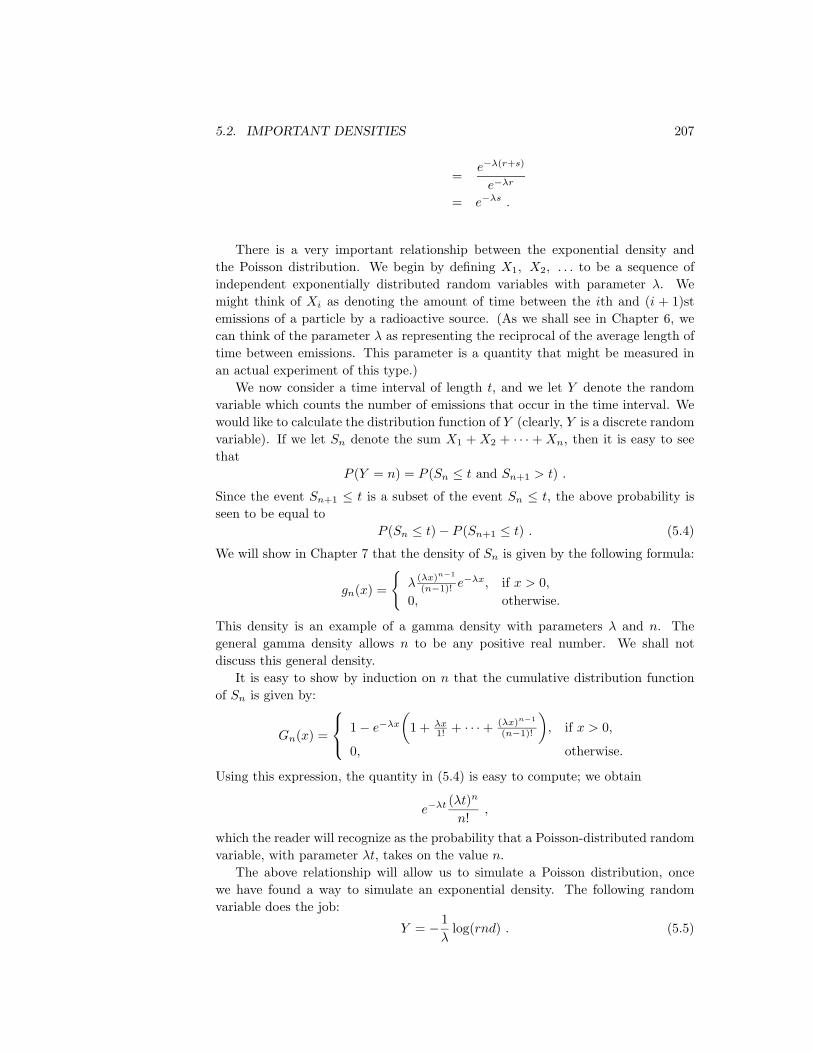
5.2. IMPORTANT DENSITIES 207
=e−λ(r+s)
e−λr
= e−λs .
There is a very important relationship between the exponential density andthe Poisson distribution. We begin by defining X1, X2, . . . to be a sequence ofindependent exponentially distributed random variables with parameter λ. Wemight think of Xi as denoting the amount of time between the ith and (i + 1)stemissions of a particle by a radioactive source. (As we shall see in Chapter 6, wecan think of the parameter λ as representing the reciprocal of the average length oftime between emissions. This parameter is a quantity that might be measured inan actual experiment of this type.)
We now consider a time interval of length t, and we let Y denote the randomvariable which counts the number of emissions that occur in the time interval. Wewould like to calculate the distribution function of Y (clearly, Y is a discrete randomvariable). If we let Sn denote the sum X1 + X2 + · · · + Xn, then it is easy to seethat
P (Y = n) = P (Sn ≤ t and Sn+1 > t) .
Since the event Sn+1 ≤ t is a subset of the event Sn ≤ t, the above probability isseen to be equal to
P (Sn ≤ t)− P (Sn+1 ≤ t) . (5.4)
We will show in Chapter 7 that the density of Sn is given by the following formula:
gn(x) =
λ (λx)n−1
(n−1)! e−λx, if x > 0,
0, otherwise.
This density is an example of a gamma density with parameters λ and n. Thegeneral gamma density allows n to be any positive real number. We shall notdiscuss this general density.
It is easy to show by induction on n that the cumulative distribution functionof Sn is given by:
Gn(x) =
1− e−λx(
1 + λx1! + · · ·+ (λx)n−1
(n−1)!
), if x > 0,
0, otherwise.
Using this expression, the quantity in (5.4) is easy to compute; we obtain
e−λt(λt)n
n!,
which the reader will recognize as the probability that a Poisson-distributed randomvariable, with parameter λt, takes on the value n.
The above relationship will allow us to simulate a Poisson distribution, oncewe have found a way to simulate an exponential density. The following randomvariable does the job:
Y = − 1λ
log(rnd) . (5.5)

208 CHAPTER 5. DISTRIBUTIONS AND DENSITIES
Using Corollary 5.2 (below), one can derive the above expression (see Exercise 3).We content ourselves for now with a short calculation that should convince thereader that the random variable Y has the required property. We have
P (Y ≤ y) = P(− 1λ
log(rnd) ≤ y)
= P (log(rnd) ≥ −λy)
= P (rnd ≥ e−λy)
= 1− e−λy .
This last expression is seen to be the cumulative distribution function of an expo-nentially distributed random variable with parameter λ.
To simulate a Poisson random variable W with parameter λ, we simply generatea sequence of values of an exponentially distributed random variable with the sameparameter, and keep track of the subtotals Sk of these values. We stop generatingthe sequence when the subtotal first exceeds λ. Assume that we find that
Sn ≤ λ < Sn+1 .
Then the value n is returned as a simulated value for W .
Example 5.7 (Queues) Suppose that customers arrive at random times at a servicestation with one server, and suppose that each customer is served immediately ifno one is ahead of him, but must wait his turn in line otherwise. How long shouldeach customer expect to wait? (We define the waiting time of a customer to be thelength of time between the time that he arrives and the time that he begins to beserved.)
Let us assume that the interarrival times between successive customers are givenby random variables X1, X2, . . . , Xn that are mutually independent and identicallydistributed with an exponential cumulative distribution function given by
FX(t) = 1− e−λt.
Let us assume, too, that the service times for successive customers are given byrandom variables Y1, Y2, . . . , Yn that again are mutually independent and identicallydistributed with another exponential cumulative distribution function given by
FY (t) = 1− e−µt.
The parameters λ and µ represent, respectively, the reciprocals of the averagetime between arrivals of customers and the average service time of the customers.Thus, for example, the larger the value of λ, the smaller the average time betweenarrivals of customers. We can guess that the length of time a customer will spendin the queue depends on the relative sizes of the average interarrival time and theaverage service time.
It is easy to verify this conjecture by simulation. The program Queue simulatesthis queueing process. Let N(t) be the number of customers in the queue at time t.

5.2. IMPORTANT DENSITIES 209
2000 4000 6000 8000 10000
10
20
30
40
50
60
2000 4000 6000 8000 10000
200
400
600
800
1000
1200 λ = 1 λ = 1µ = .9 µ = 1.1
Figure 5.7: Queue sizes.
0 10 20 30 40 50
0
0.01
0.02
0.03
0.04
0.05
0.06
0.07
Figure 5.8: Waiting times.
Then we plot N(t) as a function of t for different choices of the parameters λ andµ (see Figure 5.7).
We note that when λ < µ, then 1/λ > 1/µ, so the average interarrival time isgreater than the average service time, i.e., customers are served more quickly, onaverage, than new ones arrive. Thus, in this case, it is reasonable to expect thatN(t) remains small. However, if λ > µ then customers arrive more quickly thanthey are served, and, as expected, N(t) appears to grow without limit.
We can now ask: How long will a customer have to wait in the queue for service?To examine this question, we let Wi be the length of time that the ith customer hasto remain in the system (waiting in line and being served). Then we can presentthese data in a bar graph, using the program Queue, to give some idea of how theWi are distributed (see Figure 5.8). (Here λ = 1 and µ = 1.1.)
We see that these waiting times appear to be distributed exponentially. This isalways the case when λ < µ. The proof of this fact is too complicated to give here,but we can verify it by simulation for different choices of λ and µ, as above. 2

210 CHAPTER 5. DISTRIBUTIONS AND DENSITIES
Functions of a Random Variable
Before continuing our list of important densities, we pause to consider randomvariables which are functions of other random variables. We will prove a generaltheorem that will allow us to derive expressions such as Equation 5.5.
Theorem 5.1 Let X be a continuous random variable, and suppose that φ(x) is astrictly increasing function on the range of X. Define Y = φ(X). Suppose that Xand Y have cumulative distribution functions FX and FY respectively. Then thesefunctions are related by
FY (y) = FX(φ−1(y)).
If φ(x) is strictly decreasing on the range of X, then
FY (y) = 1− FX(φ−1(y)) .
Proof. Since φ is a strictly increasing function on the range of X, the events(X ≤ φ−1(y)) and (φ(X) ≤ y) are equal. Thus, we have
FY (y) = P (Y ≤ y)
= P (φ(X) ≤ y)
= P (X ≤ φ−1(y))
= FX(φ−1(y)) .
If φ(x) is strictly decreasing on the range of X, then we have
FY (y) = P (Y ≤ y)
= P (φ(X) ≤ y)
= P (X ≥ φ−1(y))
= 1− P (X < φ−1(y))
= 1− FX(φ−1(y)) .
This completes the proof. 2
Corollary 5.1 Let X be a continuous random variable, and suppose that φ(x) is astrictly increasing function on the range of X. Define Y = φ(X). Suppose that thedensity functions of X and Y are fX and fY , respectively. Then these functionsare related by
fY (y) = fX(φ−1(y))d
dyφ−1(y) .
If φ(x) is strictly decreasing on the range of X, then
fY (y) = −fX(φ−1(y))d
dyφ−1(y) .

5.2. IMPORTANT DENSITIES 211
Proof. This result follows from Theorem 5.1 by using the Chain Rule. 2
If the function φ is neither strictly increasing nor strictly decreasing, then thesituation is somewhat more complicated but can be treated by the same methods.For example, suppose that Y = X2, Then φ(x) = x2, and
FY (y) = P (Y ≤ y)
= P (−√y ≤ X ≤ +√y)
= P (X ≤ +√y)− P (X ≤ −√y)
= FX(√y)− FX(−√y) .
Moreover,
fY (y) =d
dyFY (y)
=d
dy(FX(
√y)− FX(−√y))
=(fX(√y) + fX(−√y)
) 12√y.
We see that in order to express FY in terms of FX when Y = φ(X), we have toexpress P (Y ≤ y) in terms of P (X ≤ x), and this process will depend in generalupon the structure of φ.
Simulation
Theorem 5.1 tells us, among other things, how to simulate on the computer a randomvariable Y with a prescribed cumulative distribution function F . We assume thatF (y) is strictly increasing for those values of y where 0 < F (y) < 1. For thispurpose, let U be a random variable which is uniformly distributed on [0, 1]. ThenU has cumulative distribution function FU (u) = u. Now, if F is the prescribedcumulative distribution function for Y , then to write Y in terms of U we first solvethe equation
F (y) = u
for y in terms of u. We obtain y = F−1(u). Note that since F is an increasingfunction this equation always has a unique solution (see Figure 5.9). Then we setZ = F−1(U) and obtain, by Theorem 5.1,
FZ(y) = FU (F (y)) = F (y) ,
since FU (u) = u. Therefore, Z and Y have the same cumulative distribution func-tion. Summarizing, we have the following.

212 CHAPTER 5. DISTRIBUTIONS AND DENSITIES
y = φ(x)
x = FY (y)
Y (y)Graph of Fx
y
1
0
Figure 5.9: Converting a uniform distribution FU into a prescribed distribution FY .
Corollary 5.2 If F (y) is a given cumulative distribution function that is strictlyincreasing when 0 < F (y) < 1 and if U is a random variable with uniform distribu-tion on [0, 1], then
Y = F−1(U)
has the cumulative distribution F (y). 2
Thus, to simulate a random variable with a given cumulative distribution F weneed only set Y = F−1(rnd).
Normal Density
We now come to the most important density function, the normal density function.We have seen in Chapter 3 that the binomial distribution functions are bell-shaped,even for moderate size values of n. We recall that a binomially-distributed randomvariable with parameters n and p can be considered to be the sum of n mutuallyindependent 0-1 random variables. A very important theorem in probability theory,called the Central Limit Theorem, states that under very general conditions, if wesum a large number of mutually independent random variables, then the distributionof the sum can be closely approximated by a certain specific continuous density,called the normal density. This theorem will be discussed in Chapter 9.
The normal density function with parameters µ and σ is defined as follows:
fX(x) =1√2πσ
e−(x−µ)2/2σ2.
The parameter µ represents the “center” of the density (and in Chapter 6, we willshow that it is the average, or expected, value of the density). The parameter σis a measure of the “spread” of the density, and thus it is assumed to be positive.(In Chapter 6, we will show that σ is the standard deviation of the density.) Wenote that it is not at all obvious that the above function is a density, i.e., that its
5.2. IMPORTANT DENSITIES 213
-4 -2 2 4
0.1
0.2
0.3
0.4
σ = 1
σ = 2
Figure 5.10: Normal density for two sets of parameter values.
integral over the real line equals 1. The cumulative distribution function is givenby the formula
FX(x) =∫ x
−∞
1√2πσ
e−(u−µ)2/2σ2du .
In Figure 5.10 we have included for comparison a plot of the normal density forthe cases µ = 0 and σ = 1, and µ = 0 and σ = 2.
One cannot write FX in terms of simple functions. This leads to several prob-lems. First of all, values of FX must be computed using numerical integration.Extensive tables exist containing values of this function (see Appendix A). Sec-ondly, we cannot write F−1
X in closed form, so we cannot use Corollary 5.2 to helpus simulate a normal random variable. For this reason, special methods have beendeveloped for simulating a normal distribution. One such method relies on the factthat if U and V are independent random variables with uniform densities on [0, 1],then the random variables
X =√−2 logU cos 2πV
andY =
√−2 logU sin 2πV
are independent, and have normal density functions with parameters µ = 0 andσ = 1. (This is not obvious, nor shall we prove it here. See Box and Muller.9)
Let Z be a normal random variable with parameters µ = 0 and σ = 1. Anormal random variable with these parameters is said to be a standard normalrandom variable. It is an important and useful fact that if we write
X = σZ + µ ,
then X is a normal random variable with parameters µ and σ. To show this, wewill use Theorem 5.1. We have φ(z) = σz + µ, φ−1(x) = (x− µ)/σ, and
FX(x) = FZ
(x− µσ
),
9G. E. P. Box and M. E. Muller, A Note on the Generation of Random Normal Deviates, Ann.of Math. Stat. 29 (1958), pgs. 610-611.

214 CHAPTER 5. DISTRIBUTIONS AND DENSITIES
fX(x) = fZ
(x− µσ
)· 1σ
=1√2πσ
e−(x−µ)2/2σ2.
The reader will note that this last expression is the density function with parametersµ and σ, as claimed.
We have seen above that it is possible to simulate a standard normal randomvariable Z. If we wish to simulate a normal random variable X with parameters µand σ, then we need only transform the simulated values for Z using the equationX = σZ + µ.
Suppose that we wish to calculate the value of a cumulative distribution functionfor the normal random variable X, with parameters µ and σ. We can reduce thiscalculation to one concerning the standard normal random variable Z as follows:
FX(x) = P (X ≤ x)
= P
(Z ≤ x− µ
σ
)= FZ
(x− µσ
).
This last expression can be found in a table of values of the cumulative distributionfunction for a standard normal random variable. Thus, we see that it is unnecessaryto make tables of normal distribution functions with arbitrary µ and σ.
The process of changing a normal random variable to a standard normal ran-dom variable is known as standardization. If X has a normal distribution withparameters µ and σ and if
Z =X − µσ
,
then Z is said to be the standardized version of X.The following example shows how we use the standardized version of a normal
random variable X to compute specific probabilities relating to X.
Example 5.8 Suppose that X is a normally distributed random variable with pa-rameters µ = 10 and σ = 3. Find the probability that X is between 4 and 16.
To solve this problem, we note that Z = (X − 10)/3 is the standardized versionof X. So, we have
P (4 ≤ X ≤ 16) = P (X ≤ 16)− P (X ≤ 4)
= FX(16)− FX(4)
= FZ
(16− 10
3
)− FZ
(4− 10
3
)= FZ(2)− FZ(−2) .

5.2. IMPORTANT DENSITIES 215
0 1 2 3 4 5
0
0.1
0.2
0.3
0.4
0.5
0.6
Figure 5.11: Distribution of dart distances in 1000 drops.
This last expression can be evaluated by using tabulated values of the standardnormal distribution function (see 12.3); when we use this table, we find that FZ(2) =.9772 and FZ(−2) = .0228. Thus, the answer is .9544.
In Chapter 6, we will see that the parameter µ is the mean, or average value, ofthe random variable X. The parameter σ is a measure of the spread of the randomvariable, and is called the standard deviation. Thus, the question asked in thisexample is of a typical type, namely, what is the probability that a random variablehas a value within two standard deviations of its average value. 2
Maxwell and Rayleigh Densities
Example 5.9 Suppose that we drop a dart on a large table top, which we consideras the xy-plane, and suppose that the x and y coordinates of the dart point areindependent and have a normal distribution with parameters µ = 0 and σ = 1.How is the distance of the point from the origin distributed?
This problem arises in physics when it is assumed that a moving particle inRn has components of the velocity that are mutually independent and normallydistributed and it is desired to find the density of the speed of the particle. Thedensity in the case n = 3 is called the Maxwell density.
The density in the case n = 2 (i.e. the dart board experiment described above)is called the Rayleigh density. We can simulate this case by picking independently apair of coordinates (x, y), each from a normal distribution with µ = 0 and σ = 1 on(−∞,∞), calculating the distance r =
√x2 + y2 of the point (x, y) from the origin,
repeating this process a large number of times, and then presenting the results in abar graph. The results are shown in Figure 5.11.

216 CHAPTER 5. DISTRIBUTIONS AND DENSITIES
Female MaleA 37 56 93B 63 60 123C 47 43 90
Below C 5 8 13152 167 319
Table 5.8: Calculus class data.
Female MaleA 44.3 48.7 93B 58.6 64.4 123C 42.9 47.1 90
Below C 6.2 6.8 13152 167 319
Table 5.9: Expected data.
We have also plotted the theoretical density
f(r) = re−r2/2 .
This will be derived in Chapter 7; see Example 7.7. 2
Chi-Squared Density
We return to the problem of independence of traits discussed in Example 5.6. Itis frequently the case that we have two traits, each of which have several differentvalues. As was seen in the example, quite a lot of calculation was needed evenin the case of two values for each trait. We now give another method for testingindependence of traits, which involves much less calculation.
Example 5.10 Suppose that we have the data shown in Table 5.8 concerninggrades and gender of students in a Calculus class. We can use the same sort ofmodel in this situation as was used in Example 5.6. We imagine that we have anurn with 319 balls of two colors, say blue and red, corresponding to females andmales, respectively. We now draw 93 balls, without replacement, from the urn.These balls correspond to the grade of A. We continue by drawing 123 balls, whichcorrespond to the grade of B. When we finish, we have four sets of balls, with eachball belonging to exactly one set. (We could have stipulated that the balls wereof four colors, corresponding to the four possible grades. In this case, we woulddraw a subset of size 152, which would correspond to the females. The balls re-maining in the urn would correspond to the males. The choice does not affect thefinal determination of whether we should reject the hypothesis of independence oftraits.)
The expected data set can be determined in exactly the same way as in Exam-ple 5.6. If we do this, we obtain the expected values shown in Table 5.9. Even if

5.2. IMPORTANT DENSITIES 217
the traits are independent, we would still expect to see some differences betweenthe numbers in corresponding boxes in the two tables. However, if the differencesare large, then we might suspect that the two traits are not independent. In Ex-ample 5.6, we used the probability distribution of the various possible data sets tocompute the probability of finding a data set that differs from the expected dataset by at least as much as the actual data set does. We could do the same in thiscase, but the amount of computation is enormous.
Instead, we will describe a single number which does a good job of measuringhow far a given data set is from the expected one. To quantify how far apart the twosets of numbers are, we could sum the squares of the differences of the correspondingnumbers. (We could also sum the absolute values of the differences, but we wouldnot want to sum the differences.) Suppose that we have data in which we expectto see 10 objects of a certain type, but instead we see 18, while in another case weexpect to see 50 objects of a certain type, but instead we see 58. Even though thetwo differences are about the same, the first difference is more surprising than thesecond, since the expected number of outcomes in the second case is quite a bitlarger than the expected number in the first case. One way to correct for this isto divide the individual squares of the differences by the expected number for thatbox. Thus, if we label the values in the eight boxes in the first table by Oi (forobserved values) and the values in the eight boxes in the second table by Ei (forexpected values), then the following expression might be a reasonable one to use tomeasure how far the observed data is from what is expected:
8∑i=1
(Oi − Ei)2
Ei.
This expression is a random variable, which is usually denoted by the symbol χ2,pronounced “ki-squared.” It is called this because, under the assumption of inde-pendence of the two traits, the density of this random variable can be computed andis approximately equal to a density called the chi-squared density. We choose notto give the explicit expression for this density, since it involves the gamma function,which we have not discussed. The chi-squared density is, in fact, a special case ofthe general gamma density.
In applying the chi-squared density, tables of values of this density are used, asin the case of the normal density. The chi-squared density has one parameter n,which is called the number of degrees of freedom. The number n is usually easy todetermine from the problem at hand. For example, if we are checking two traits forindependence, and the two traits have a and b values, respectively, then the numberof degrees of freedom of the random variable χ2 is (a−1)(b−1). So, in the exampleat hand, the number of degrees of freedom is 3.
We recall that in this example, we are trying to test for independence of thetwo traits of gender and grades. If we assume these traits are independent, thenthe ball-and-urn model given above gives us a way to simulate the experiment.Using a computer, we have performed 1000 experiments, and for each one, we havecalculated a value of the random variable χ2. The results are shown in Figure 5.12,together with the chi-squared density function with three degrees of freedom.

218 CHAPTER 5. DISTRIBUTIONS AND DENSITIES
0 2 4 6 8 10 12
0
0.05
0.1
0.15
0.2
Figure 5.12: Chi-squared density with three degrees of freedom.
As we stated above, if the value of the random variable χ2 is large, then wewould tend not to believe that the two traits are independent. But how large islarge? The actual value of this random variable for the data above is 4.13. InFigure 5.12, we have shown the chi-squared density with 3 degrees of freedom. Itcan be seen that the value 4.13 is larger than most of the values taken on by thisrandom variable.
Typically, a statistician will compute the value v of the random variable χ2,just as we have done. Then, by looking in a table of values of the chi-squareddensity, a value v0 is determined which is only exceeded 5% of the time. If v ≥ v0,the statistician rejects the hypothesis that the two traits are independent. In thepresent case, v0 = 7.815, so we would not reject the hypothesis that the two traitsare independent. 2
Cauchy Density
The following example is from Feller.10
Example 5.11 Suppose that a mirror is mounted on a vertical axis, and is freeto revolve about that axis. The axis of the mirror is 1 foot from a straight wallof infinite length. A pulse of light is shown onto the mirror, and the reflected rayhits the wall. Let φ be the angle between the reflected ray and the line that isperpendicular to the wall and that runs through the axis of the mirror. We assumethat φ is uniformly distributed between −π/2 and π/2. Let X represent the distancebetween the point on the wall that is hit by the reflected ray and the point on thewall that is closest to the axis of the mirror. We now determine the density of X.
Let B be a fixed positive quantity. Then X ≥ B if and only if tan(φ) ≥ B,which happens if and only if φ ≥ arctan(B). This happens with probability
π/2− arctan(B)π
.
10W. Feller, An Introduction to Probability Theory and Its Applications,, vol. 2, (New York:Wiley, 1966)

5.2. IMPORTANT DENSITIES 219
Thus, for positive B, the cumulative distribution function of X is
F (B) = 1− π/2− arctan(B)π
.
Therefore, the density function for positive B is
f(B) =1
π(1 +B2).
Since the physical situation is symmetric with respect to φ = 0, it is easy to seethat the above expression for the density is correct for negative values of B as well.
The Law of Large Numbers, which we will discuss in Chapter 8, states thatin many cases, if we take the average of independent values of a random variable,then the average approaches a specific number as the number of values increases.It turns out that if one does this with a Cauchy-distributed random variable, theaverage does not approach any specific number. 2
Exercises
1 Choose a number U from the unit interval [0, 1] with uniform distribution.Find the cumulative distribution and density for the random variables
(a) Y = U + 2.
(b) Y = U3.
2 Choose a number U from the interval [0, 1] with uniform distribution. Findthe cumulative distribution and density for the random variables
(a) Y = 1/(U + 1).
(b) Y = log(U + 1).
3 Use Corollary 5.2 to derive the expression for the random variable given inEquation 5.5. Hint : The random variables 1 − rnd and rnd are identicallydistributed.
4 Suppose we know a random variable Y as a function of the uniform randomvariable U : Y = φ(U), and suppose we have calculated the cumulative dis-tribution function FY (y) and thence the density fY (y). How can we checkwhether our answer is correct? An easy simulation provides the answer: Makea bar graph of Y = φ(rnd) and compare the result with the graph of fY (y).These graphs should look similar. Check your answers to Exercises 1 and 2by this method.
5 Choose a number U from the interval [0, 1] with uniform distribution. Findthe cumulative distribution and density for the random variables
(a) Y = |U − 1/2|.(b) Y = (U − 1/2)2.

220 CHAPTER 5. DISTRIBUTIONS AND DENSITIES
6 Check your results for Exercise 5 by simulation as described in Exercise 4.
7 Explain how you can generate a random variable whose cumulative distribu-tion function is
F (x) =
0, if x < 0,x2, if 0 ≤ x ≤ 1,1, if x > 1.
8 Write a program to generate a sample of 1000 random outcomes each of whichis chosen from the distribution given in Exercise 7. Plot a bar graph of yourresults and compare this empirical density with the density for the cumulativedistribution given in Exercise 7.
9 Let U , V be random numbers chosen independently from the interval [0, 1]with uniform distribution. Find the cumulative distribution and density ofeach of the variables
(a) Y = U + V .
(b) Y = |U − V |.
10 Let U , V be random numbers chosen independently from the interval [0, 1].Find the cumulative distribution and density for the random variables
(a) Y = max(U, V ).
(b) Y = min(U, V ).
11 Write a program to simulate the random variables of Exercises 9 and 10 andplot a bar graph of the results. Compare the resulting empirical density withthe density found in Exercises 9 and 10.
12 A number U is chosen at random in the interval [0, 1]. Find the probabilitythat
(a) R = U2 < 1/4.
(b) S = U(1− U) < 1/4.
(c) T = U/(1− U) < 1/4.
13 Find the cumulative distribution function F and the density function f foreach of the random variables R, S, and T in Exercise 12.
14 A point P in the unit square has coordinates X and Y chosen at random inthe interval [0, 1]. Let D be the distance from P to the nearest edge of thesquare, and E the distance to the nearest corner. What is the probabilitythat
(a) D < 1/4?
(b) E < 1/4?
15 In Exercise 14 find the cumulative distribution F and density f for the randomvariable D.

5.2. IMPORTANT DENSITIES 221
16 Let X be a random variable with density function
fX(x) =cx(1− x), if 0 < x < 1,0, otherwise.
(a) What is the value of c?
(b) What is the cumulative distribution function FX for X?
(c) What is the probability that X < 1/4?
17 Let X be a random variable with cumulative distribution function
F (x) =
0, if x < 0,sin2(πx/2), if 0 ≤ x ≤ 1,1, if 1 < x.
(a) What is the density function fX for X?
(b) What is the probability that X < 1/4?
18 Let X be a random variable with cumulative distribution function FX , andlet Y = X + b, Z = aX, and W = aX + b, where a and b are any constants.Find the cumulative distribution functions FY , FZ , and FW . Hint : The casesa > 0, a = 0, and a < 0 require different arguments.
19 Let X be a random variable with density function fX , and let Y = X + b,Z = aX, and W = aX + b, where a 6= 0. Find the density functions fY , fZ ,and fW . (See Exercise 18.)
20 Let X be a random variable uniformly distributed over [c, d], and let Y =aX + b. For what choice of a and b is Y uniformly distributed over [0, 1]?
21 Let X be a random variable with cumulative distribution function F strictlyincreasing on the range of X. Let Y = F (X). Show that Y is uniformlydistributed in the interval [0, 1]. (The formula X = F−1(Y ) then tells us howto construct X from a uniform random variable Y .)
22 Let X be a random variable with cumulative distribution function F . Themedian of X is the value m for which F (m) = 1/2. Then X < m withprobability 1/2 and X > m with probability 1/2. Find m if X is
(a) uniformly distributed over the interval [a, b].
(b) normally distributed with parameters µ and σ.
(c) exponentially distributed with parameter λ.
23 Let X be a random variable with density function fX . The mean of X isthe value µ =
∫xfx(x) dx. Then µ gives an average value for X (see Sec-
tion 6.3). Find µ if X is distributed uniformly, normally, or exponentially, asin Exercise 22.

222 CHAPTER 5. DISTRIBUTIONS AND DENSITIES
Test Score Letter gradeµ+ σ < x Aµ < x < µ+ σ Bµ− σ < x < µ Cµ− 2σ < x < µ− σ Dx < µ− 2σ F
Table 5.10: Grading on the curve.
24 Let X be a random variable with density function fX . The mode of X is thevalue M for which f(M) is maximum. Then values of X near M are mostlikely to occur. Find M if X is distributed normally or exponentially, as inExercise 22. What happens if X is distributed uniformly?
25 Let X be a random variable normally distributed with parameters µ = 70,σ = 10. Estimate
(a) P (X > 50).
(b) P (X < 60).
(c) P (X > 90).
(d) P (60 < X < 80).
26 Bridies’ Bearing Works manufactures bearing shafts whose diameters are nor-mally distributed with parameters µ = 1, σ = .002. The buyer’s specificationsrequire these diameters to be 1.000 ± .003 cm. What fraction of the manu-facturer’s shafts are likely to be rejected? If the manufacturer improves herquality control, she can reduce the value of σ. What value of σ will ensurethat no more than 1 percent of her shafts are likely to be rejected?
27 A final examination at Podunk University is constructed so that the testscores are approximately normally distributed, with parameters µ and σ. Theinstructor assigns letter grades to the test scores as shown in Table 5.10 (thisis the process of “grading on the curve”).
What fraction of the class gets A, B, C, D, F?
28 (Ross11) An expert witness in a paternity suit testifies that the length (indays) of a pregnancy, from conception to delivery, is approximately normallydistributed, with parameters µ = 270, σ = 10. The defendant in the suit isable to prove that he was out of the country during the period from 290 to 240days before the birth of the child. What is the probability that the defendantwas in the country when the child was conceived?
29 Suppose that the time (in hours) required to repair a car is an exponentiallydistributed random variable with parameter λ = 1/2. What is the probabil-ity that the repair time exceeds 4 hours? If it exceeds 4 hours what is theprobability that it exceeds 8 hours?
11S. Ross, A First Course in Probability Theory, 2d ed. (New York: Macmillan, 1984).

5.2. IMPORTANT DENSITIES 223
30 Suppose that the number of years a car will run is exponentially distributedwith parameter µ = 1/4. If Prosser buys a used car today, what is theprobability that it will still run after 4 years?
31 Let U be a uniformly distributed random variable on [0, 1]. What is theprobability that the equation
x2 + 4Ux+ 1 = 0
has two distinct real roots x1 and x2?
32 Write a program to simulate the random variables whose densities are givenby the following, making a suitable bar graph of each and comparing the exactdensity with the bar graph.
(a) fX(x) = e−x on [0,∞) (but just do it on [0, 10]).
(b) fX(x) = 2x on [0, 1].
(c) fX(x) = 3x2 on [0, 1].
(d) fX(x) = 4|x− 1/2| on [0, 1].
33 Suppose we are observing a process such that the time between occurrencesis exponentially distributed with λ = 1/30 (i.e., the average time betweenoccurrences is 30 minutes). Suppose that the process starts at a certain timeand we start observing the process 3 hours later. Write a program to simulatethis process. Let T denote the length of time that we have to wait, after westart our observation, for an occurrence. Have your program keep track of T .What is an estimate for the average value of T?
34 Jones puts in two new lightbulbs: a 60 watt bulb and a 100 watt bulb. Itis claimed that the lifetime of the 60 watt bulb has an exponential densitywith average lifetime 200 hours (λ = 1/200). The 100 watt bulb also has anexponential density but with average lifetime of only 100 hours (λ = 1/100).Jones wonders what is the probability that the 100 watt bulb will outlast the60 watt bulb.
If X and Y are two independent random variables with exponential densitiesf(x) = λe−λx and g(x) = µe−µx, respectively, then the probability that X isless than Y is given by
P (X < Y ) =∫ ∞
0
f(x)(1−G(x)) dx,
where G(x) is the cumulative distribution function for g(x). Explain why thisis the case. Use this to show that
P (X < Y ) =λ
λ+ µ
and to answer Jones’s question.
224 CHAPTER 5. DISTRIBUTIONS AND DENSITIES
35 Consider the simple queueing process of Example 5.7. Suppose that you watchthe size of the queue. If there are j people in the queue the next time thequeue size changes it will either decrease to j − 1 or increase to j + 1. Usethe result of Exercise 34 to show that the probability that the queue sizedecreases to j − 1 is µ/(µ + λ) and the probability that it increases to j + 1is λ/(µ + λ). When the queue size is 0 it can only increase to 1. Write aprogram to simulate the queue size. Use this simulation to help formulate aconjecture containing conditions on µ and λ that will ensure that the queuewill have times when it is empty.
36 Let X be a random variable having an exponential density with parameter λ.Find the density for the random variable Y = rX, where r is a positive realnumber.
37 Let X be a random variable having a normal density and consider the randomvariable Y = eX . Then Y has a log normal density. Find this density of Y .
38 Let X1 and X2 be independent random variables and for i = 1, 2, let Yi =φi(Xi), where φi is strictly increasing on the range of Xi. Show that Y1 andY2 are independent. Note that the same result is true without the assumptionthat the φi’s are strictly increasing, but the proof is more difficult.

Chapter 6
Expected Value and Variance
6.1 Expected Value of Discrete Random Variables
When a large collection of numbers is assembled, as in a census, we are usuallyinterested not in the individual numbers, but rather in certain descriptive quantitiessuch as the average or the median. In general, the same is true for the probabilitydistribution of a numerically-valued random variable. In this and in the next section,we shall discuss two such descriptive quantities: the expected value and the variance.Both of these quantities apply only to numerically-valued random variables, and sowe assume, in these sections, that all random variables have numerical values. Togive some intuitive justification for our definition, we consider the following game.
Average Value
A die is rolled. If an odd number turns up, we win an amount equal to this number;if an even number turns up, we lose an amount equal to this number. For example,if a two turns up we lose 2, and if a three comes up we win 3. We want to decide ifthis is a reasonable game to play. We first try simulation. The program Die carriesout this simulation.
The program prints the frequency and the relative frequency with which eachoutcome occurs. It also calculates the average winnings. We have run the programtwice. The results are shown in Table 6.1.
In the first run we have played the game 100 times. In this run our average gainis −.57. It looks as if the game is unfavorable, and we wonder how unfavorable itreally is. To get a better idea, we have played the game 10,000 times. In this caseour average gain is −.4949.
We note that the relative frequency of each of the six possible outcomes is quiteclose to the probability 1/6 for this outcome. This corresponds to our frequencyinterpretation of probability. It also suggests that for very large numbers of plays,our average gain should be
µ = 1(1
6
)− 2(1
6
)+ 3(1
6
)− 4(1
6
)+ 5(1
6
)− 6(1
6
)225

226 CHAPTER 6. EXPECTED VALUE AND VARIANCE
n = 100 n = 10000Winning Frequency Relative Frequency Relative
Frequency Frequency1 17 .17 1681 .1681-2 17 .17 1678 .16783 16 .16 1626 .1626-4 18 .18 1696 .16965 16 .16 1686 .1686-6 16 .16 1633 .1633
Table 6.1: Frequencies for dice game.
=96− 12
6= −3
6= −.5 .
This agrees quite well with our average gain for 10,000 plays.We note that the value we have chosen for the average gain is obtained by taking
the possible outcomes, multiplying by the probability, and adding the results. Thissuggests the following definition for the expected outcome of an experiment.
Expected Value
Definition 6.1 Let X be a numerically-valued discrete random variable with sam-ple space Ω and distribution function m(x). The expected value E(X) is definedby
E(X) =∑x∈Ω
xm(x) ,
provided this sum converges absolutely. We often refer to the expected value asthe mean, and denote E(X) by µ for short. If the above sum does not convergeabsolutely, then we say that X does not have an expected value. 2
Example 6.1 Let an experiment consist of tossing a fair coin three times. LetX denote the number of heads which appear. Then the possible values of X are0, 1, 2 and 3. The corresponding probabilities are 1/8, 3/8, 3/8, and 1/8. Thus, theexpected value of X equals
0(
18
)+ 1(
38
)+ 2(
38
)+ 3(
18
)=
32.
Later in this section we shall see a quicker way to compute this expected value,based on the fact that X can be written as a sum of simpler random variables. 2
Example 6.2 Suppose that we toss a fair coin until a head first comes up, and letX represent the number of tosses which were made. Then the possible values of Xare 1, 2, . . ., and the distribution function of X is defined by
m(i) =12i.

6.1. EXPECTED VALUE 227
(This is just the geometric distribution with parameter 1/2.) Thus, we have
E(X) =∞∑i=1
i12i
=∞∑i=1
12i
+∞∑i=2
12i
+ · · ·
= 1 +12
+122
+ · · ·= 2 .
2
Example 6.3 (Example 6.2 continued) Suppose that we flip a coin until a headfirst appears, and if the number of tosses equals n, then we are paid 2n dollars.What is the expected value of the payment?
We let Y represent the payment. Then,
P (Y = 2n) =12n
,
for n ≥ 1. Thus,
E(Y ) =∞∑n=1
2n12n
,
which is a divergent sum. Thus, Y has no expectation. This example is calledthe St. Petersburg Paradox . The fact that the above sum is infinite suggests thata player should be willing to pay any fixed amount per game for the privilege ofplaying this game. The reader is asked to consider how much he or she would bewilling to pay for this privilege. It is unlikely that the reader’s answer is more than10 dollars; therein lies the paradox.
In the early history of probability, various mathematicians gave ways to resolvethis paradox. One idea (due to G. Cramer) consists of assuming that the amountof money in the world is finite. He thus assumes that there is some fixed value ofn such that if the number of tosses equals or exceeds n, the payment is 2n dollars.The reader is asked to show in Exercise 20 that the expected value of the paymentis now finite.
Daniel Bernoulli and Cramer also considered another way to assign value tothe payment. Their idea was that the value of a payment is some function of thepayment; such a function is now called a utility function. Examples of reasonableutility functions might include the square-root function or the logarithm function.In both cases, the value of 2n dollars is less than twice the value of n dollars. Itcan easily be shown that in both cases, the expected utility of the payment is finite(see Exercise 20). 2

228 CHAPTER 6. EXPECTED VALUE AND VARIANCE
Example 6.4 Let T be the time for the first success in a Bernoulli trials process.Then we take as sample space Ω the integers 1, 2, . . . and assign the geometricdistribution
m(j) = P (T = j) = qj−1p .
Thus,
E(T ) = 1 · p+ 2qp+ 3q2p+ · · ·= p(1 + 2q + 3q2 + · · ·) .
Now if |x| < 1, then
1 + x+ x2 + x3 + · · · = 11− x .
Differentiating this formula, we get
1 + 2x+ 3x2 + · · · = 1(1− x)2
,
soE(T ) =
p
(1− q)2=
p
p2=
1p.
In particular, we see that if we toss a fair coin a sequence of times, the expectedtime until the first heads is 1/(1/2) = 2. If we roll a die a sequence of times, theexpected number of rolls until the first six is 1/(1/6) = 6. 2
Interpretation of Expected Value
In statistics, one is frequently concerned with the average value of a set of data.The following example shows that the ideas of average value and expected value arevery closely related.
Example 6.5 The heights, in inches, of the women on the Swarthmore basketballteam are 5’ 9”, 5’ 9”, 5’ 6”, 5’ 8”, 5’ 11”, 5’ 5”, 5’ 7”, 5’ 6”, 5’ 6”, 5’ 7”, 5’ 10”, and6’ 0”.
A statistician would compute the average height (in inches) as follows:
69 + 69 + 66 + 68 + 71 + 65 + 67 + 66 + 66 + 67 + 70 + 7212
= 67.9 .
One can also interpret this number as the expected value of a random variable. Tosee this, let an experiment consist of choosing one of the women at random, and letX denote her height. Then the expected value of X equals 67.9. 2
Of course, just as with the frequency interpretation of probability, to interpretexpected value as an average outcome requires further justification. We know thatfor any finite experiment the average of the outcomes is not predictable. However,we shall eventually prove that the average will usually be close to E(X) if we repeatthe experiment a large number of times. We first need to develop some properties ofthe expected value. Using these properties, and those of the concept of the variance
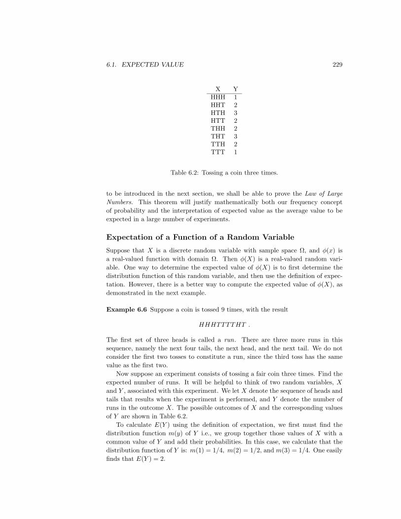
6.1. EXPECTED VALUE 229
X YHHH 1HHT 2HTH 3HTT 2THH 2THT 3TTH 2TTT 1
Table 6.2: Tossing a coin three times.
to be introduced in the next section, we shall be able to prove the Law of LargeNumbers. This theorem will justify mathematically both our frequency conceptof probability and the interpretation of expected value as the average value to beexpected in a large number of experiments.
Expectation of a Function of a Random Variable
Suppose that X is a discrete random variable with sample space Ω, and φ(x) isa real-valued function with domain Ω. Then φ(X) is a real-valued random vari-able. One way to determine the expected value of φ(X) is to first determine thedistribution function of this random variable, and then use the definition of expec-tation. However, there is a better way to compute the expected value of φ(X), asdemonstrated in the next example.
Example 6.6 Suppose a coin is tossed 9 times, with the result
HHHTTTTHT .
The first set of three heads is called a run. There are three more runs in thissequence, namely the next four tails, the next head, and the next tail. We do notconsider the first two tosses to constitute a run, since the third toss has the samevalue as the first two.
Now suppose an experiment consists of tossing a fair coin three times. Find theexpected number of runs. It will be helpful to think of two random variables, Xand Y , associated with this experiment. We let X denote the sequence of heads andtails that results when the experiment is performed, and Y denote the number ofruns in the outcome X. The possible outcomes of X and the corresponding valuesof Y are shown in Table 6.2.
To calculate E(Y ) using the definition of expectation, we first must find thedistribution function m(y) of Y i.e., we group together those values of X with acommon value of Y and add their probabilities. In this case, we calculate that thedistribution function of Y is: m(1) = 1/4, m(2) = 1/2, and m(3) = 1/4. One easilyfinds that E(Y ) = 2.

230 CHAPTER 6. EXPECTED VALUE AND VARIANCE
Now suppose we didn’t group the values of X with a common Y -value, butinstead, for each X-value x, we multiply the probability of x and the correspondingvalue of Y , and add the results. We obtain
1(
18
)+ 2(
18
)+ 3(
18
)+ 2(
18
)+ 2(
18
)+ 3(
18
)+ 2(
18
)+ 1(
18
),
which equals 2.This illustrates the following general principle. If X and Y are two random
variables, and Y can be written as a function of X, then one can compute theexpected value of Y using the distribution function of X. 2
Theorem 6.1 If X is a discrete random variable with sample space Ω and distri-bution function m(x), and if φ : Ω→ R is a function, then
E(φ(X)) =∑x∈Ω
φ(x)m(x) ,
provided the series converges absolutely. 2
The proof of this theorem is straightforward, involving nothing more than group-ing values of X with a common Y -value, as in Example 6.6.
The Sum of Two Random Variables
Many important results in probability theory concern sums of random variables.We first consider what it means to add two random variables.
Example 6.7 We flip a coin and let X have the value 1 if the coin comes up headsand 0 if the coin comes up tails. Then, we roll a die and let Y denote the face thatcomes up. What does X + Y mean, and what is its distribution? This questionis easily answered in this case, by considering, as we did in Chapter 4, the jointrandom variable Z = (X,Y ), whose outcomes are ordered pairs of the form (x, y),where 0 ≤ x ≤ 1 and 1 ≤ y ≤ 6. The description of the experiment makes itreasonable to assume that X and Y are independent, so the distribution functionof Z is uniform, with 1/12 assigned to each outcome. Now it is an easy matter tofind the set of outcomes of X + Y , and its distribution function. 2
In Example 6.1, the random variable X denoted the number of heads whichoccur when a fair coin is tossed three times. It is natural to think of X as thesum of the random variables X1, X2, X3, where Xi is defined to be 1 if the ith tosscomes up heads, and 0 if the ith toss comes up tails. The expected values of theXi’s are extremely easy to compute. It turns out that the expected value of X canbe obtained by simply adding the expected values of the Xi’s. This fact is statedin the following theorem.

6.1. EXPECTED VALUE 231
Theorem 6.2 Let X and Y be random variables with finite expected values. Then
E(X + Y ) = E(X) + E(Y ) ,
and if c is any constant, then
E(cX) = cE(X) .
Proof. Let the sample spaces of X and Y be denoted by ΩX and ΩY , and supposethat
ΩX = x1, x2, . . .
andΩY = y1, y2, . . . .
Then we can consider the random variable X + Y to be the result of applying thefunction φ(x, y) = x+y to the joint random variable (X,Y ). Then, by Theorem 6.1,we have
E(X + Y ) =∑j
∑k
(xj + yk)P (X = xj , Y = yk)
=∑j
∑k
xjP (X = xj , Y = yk) +∑j
∑k
ykP (X = xj , Y = yk)
=∑j
xjP (X = xj) +∑k
ykP (Y = yk) .
The last equality follows from the fact that∑k
P (X = xj , Y = yk) = P (X = xj)
and ∑j
P (X = xj , Y = yk) = P (Y = yk) .
Thus,E(X + Y ) = E(X) + E(Y ) .
If c is any constant,
E(cX) =∑j
cxjP (X = xj)
= c∑j
xjP (X = xj)
= cE(X) .
2

232 CHAPTER 6. EXPECTED VALUE AND VARIANCE
X Ya b c 3a c b 1b a c 1b c a 0c a b 0c b a 1
Table 6.3: Number of fixed points.
It is easy to prove by mathematical induction that the expected value of the sumof any finite number of random variables is the sum of the expected values of theindividual random variables.
It is important to note that mutual independence of the summands was notneeded as a hypothesis in the Theorem 6.2 and its generalization. The fact thatexpectations add, whether or not the summands are mutually independent, is some-times referred to as the First Fundamental Mystery of Probability.
Example 6.8 Let Y be the number of fixed points in a random permutation ofthe set a, b, c. To find the expected value of Y , it is helpful to consider the basicrandom variable associated with this experiment, namely the random variable Xwhich represents the random permutation. There are six possible outcomes of X,and we assign to each of them the probability 1/6 see Table 6.3. Then we cancalculate E(Y ) using Theorem 6.1, as
3(1
6
)+ 1(1
6
)+ 1(1
6
)+ 0(1
6
)+ 0(1
6
)+ 1(1
6
)= 1 .
We now give a very quick way to calculate the average number of fixed pointsin a random permutation of the set 1, 2, 3, . . . , n. Let Z denote the randompermutation. For each i, 1 ≤ i ≤ n, let Xi equal 1 if Z fixes i, and 0 otherwise. Soif we let F denote the number of fixed points in Z, then
F = X1 +X2 + · · ·+Xn .
Therefore, Theorem 6.2 implies that
E(F ) = E(X1) + E(X2) + · · ·+ E(Xn) .
But it is easy to see that for each i,
E(Xi) =1n,
soE(F ) = 1 .
This method of calculation of the expected value is frequently very useful. It applieswhenever the random variable in question can be written as a sum of simpler randomvariables. We emphasize again that it is not necessary that the summands bemutually independent. 2

6.1. EXPECTED VALUE 233
Bernoulli Trials
Theorem 6.3 Let Sn be the number of successes in n Bernoulli trials with prob-ability p for success on each trial. Then the expected number of successes is np.That is,
E(Sn) = np .
Proof. Let Xj be a random variable which has the value 1 if the jth outcome is asuccess and 0 if it is a failure. Then, for each Xj ,
E(Xj) = 0 · (1− p) + 1 · p = p .
SinceSn = X1 +X2 + · · ·+Xn ,
and the expected value of the sum is the sum of the expected values, we have
E(Sn) = E(X1) + E(X2) + · · ·+ E(Xn)
= np .
2
Poisson Distribution
Recall that the Poisson distribution with parameter λ was obtained as a limit ofbinomial distributions with parameters n and p, where it was assumed that np = λ,and n→∞. Since for each n, the corresponding binomial distribution has expectedvalue λ, it is reasonable to guess that the expected value of a Poisson distributionwith parameter λ also has expectation equal to λ. This is in fact the case, and thereader is invited to show this (see Exercise 21).
Independence
If X and Y are two random variables, it is not true in general that E(X · Y ) =E(X)E(Y ). However, this is true if X and Y are independent.
Theorem 6.4 If X and Y are independent random variables, then
E(X · Y ) = E(X)E(Y ) .
Proof. Suppose thatΩX = x1, x2, . . .
andΩY = y1, y2, . . .
234 CHAPTER 6. EXPECTED VALUE AND VARIANCE
are the sample spaces of X and Y , respectively. Using Theorem 6.1, we have
E(X · Y ) =∑j
∑k
xjykP (X = xj , Y = yk) .
But if X and Y are independent,
P (X = xj , Y = yk) = P (X = xj)P (Y = yk) .
Thus,
E(X · Y ) =∑j
∑k
xjykP (X = xj)P (Y = yk)
=
∑j
xjP (X = xj)
(∑k
ykP (Y = yk)
)= E(X)E(Y ) .
2
Example 6.9 A coin is tossed twice. Xi = 1 if the ith toss is heads and 0 otherwise.We know that X1 and X2 are independent. They each have expected value 1/2.Thus E(X1 ·X2) = E(X1)E(X2) = (1/2)(1/2) = 1/4. 2
We next give a simple example to show that the expected values need not mul-tiply if the random variables are not independent.
Example 6.10 Consider a single toss of a coin. We define the random variable Xto be 1 if heads turns up and 0 if tails turns up, and we set Y = 1 − X. ThenE(X) = E(Y ) = 1/2. But X · Y = 0 for either outcome. Hence, E(X · Y ) = 0 6=E(X)E(Y ). 2
We return to our records example of Section 3.1 for another application of theresult that the expected value of the sum of random variables is the sum of theexpected values of the individual random variables.
Records
Example 6.11 We start keeping snowfall records this year and want to find theexpected number of records that will occur in the next n years. The first year isnecessarily a record. The second year will be a record if the snowfall in the secondyear is greater than that in the first year. By symmetry, this probability is 1/2.More generally, let Xj be 1 if the jth year is a record and 0 otherwise. To findE(Xj), we need only find the probability that the jth year is a record. But therecord snowfall for the first j years is equally likely to fall in any one of these years,

6.1. EXPECTED VALUE 235
so E(Xj) = 1/j. Therefore, if Sn is the total number of records observed in thefirst n years,
E(Sn) = 1 +12
+13
+ · · ·+ 1n.
This is the famous divergent harmonic series. It is easy to show that
E(Sn) ∼ logn
as n→∞.Therefore, in ten years the expected number of records is approximately log 10 =
2.3; the exact value is the sum of the first ten terms of the harmonic series whichis 2.9. We see that, even for such a small value as n = 10, logn is not a badapproximation. 2
Craps
Example 6.12 In the game of craps, the player makes a bet and rolls a pair ofdice. If the sum of the numbers is 7 or 11 the player wins, if it is 2, 3, or 12 theplayer loses. If any other number results, say r, then r becomes the player’s pointand he continues to roll until either r or 7 occurs. If r comes up first he wins, andif 7 comes up first he loses. The program Craps simulates playing this game anumber of times.
We have run the program for 1000 plays in which the player bets 1 dollar eachtime. The player’s average winnings were −.006. The game of craps would seemto be only slightly unfavorable. Let us calculate the expected winnings on a singleplay and see if this is the case. We construct a two-stage tree measure as shown inFigure 6.1.
The first stage represents the possible sums for his first roll. The second stagerepresents the possible outcomes for the game if it has not ended on the first roll. Inthis stage we are representing the possible outcomes of a sequence of rolls requiredto determine the final outcome. The branch probabilities for the first stage arecomputed in the usual way assuming all 36 possibilites for outcomes for the pair ofdice are equally likely. For the second stage we assume that the game will eventuallyend, and we compute the conditional probabilities for obtaining either the point ora 7. For example, assume that the player’s point is 6. Then the game will end whenone of the eleven pairs, (1, 5), (2, 4), (3, 3), (4, 2), (5, 1), (1, 6), (2, 5), (3, 4), (4, 3),(5, 2), (6, 1), occurs. We assume that each of these possible pairs has the sameprobability. Then the player wins in the first five cases and loses in the last six.Thus the probability of winning is 5/11 and the probability of losing is 6/11. Fromthe path probabilities, we can find the probability that the player wins 1 dollar; itis 244/495. The probability of losing is then 251/495. Thus if X is his winning fora dollar bet,
E(X) = 1(244
495
)+ (−1)
(251495
)= − 7
495≈ −.0141 .

236 CHAPTER 6. EXPECTED VALUE AND VARIANCE
W
L
W
L
W
L
W
L
W
L
W
L
(2,3,12) L
10
9
8
6
5
4
(7,11) W
1/3
2/3
2/5
3/5
5/11
6/11
5/11
6/11
2/5
3/5
1/3
2/3
2/9
1/12
1/9
5/36
5/36
1/9
1/12
1/9
1/36
2/36
2/45
3/45
25/396
30/396
25/396
30/396
2/45
3/45
1/36
2/36
Figure 6.1: Tree measure for craps.

6.1. EXPECTED VALUE 237
The game is unfavorable, but only slightly. The player’s expected gain in n plays is−n(.0141). If n is not large, this is a small expected loss for the player. The casinomakes a large number of plays and so can afford a small average gain per play andstill expect a large profit. 2
Roulette
Example 6.13 In Las Vegas, a roulette wheel has 38 slots numbered 0, 00, 1, 2,. . . , 36. The 0 and 00 slots are green, and half of the remaining 36 slots are redand half are black. A croupier spins the wheel and throws an ivory ball. If you bet1 dollar on red, you win 1 dollar if the ball stops in a red slot, and otherwise youlose a dollar. We wish to calculate the expected value of your winnings, if you bet1 dollar on red.
Let X be the random variable which denotes your winnings in a 1 dollar bet onred in Las Vegas roulette. Then the distribution of X is given by
mX =(−1 1
20/38 18/38
),
and one can easily calculate (see Exercise 5) that
E(X) ≈ −.0526 .
We now consider the roulette game in Monte Carlo, and follow the treatmentof Sagan.1 In the roulette game in Monte Carlo there is only one 0. If you bet 1franc on red and a 0 turns up, then, depending upon the casino, one or more of thefollowing options may be offered:(a) You get 1/2 of your bet back, and the casino gets the other half of your bet.(b) Your bet is put “in prison,” which we will denote by P1. If red comes up onthe next turn, you get your bet back (but you don’t win any money). If black or 0comes up, you lose your bet.(c) Your bet is put in prison P1, as before. If red comes up on the next turn, youget your bet back, and if black comes up on the next turn, then you lose your bet.If a 0 comes up on the next turn, then your bet is put into double prison, which wewill denote by P2. If your bet is in double prison, and if red comes up on the nextturn, then your bet is moved back to prison P1 and the game proceeds as before.If your bet is in double prison, and if black or 0 come up on the next turn, thenyou lose your bet. We refer the reader to Figure 6.2, where a tree for this option isshown. In this figure, S is the starting position, W means that you win your bet,L means that you lose your bet, and E means that you break even.
It is interesting to compare the expected winnings of a 1 franc bet on red, undereach of these three options. We leave the first two calculations as an exercise (seeExercise 37). Suppose that you choose to play alternative (c). The calculation forthis case illustrates the way that the early French probabilists worked problems likethis.
1H. Sagan, Markov Chains in Monte Carlo, Math. Mag., vol. 54, no. 1 (1981), pp. 3-10.

238 CHAPTER 6. EXPECTED VALUE AND VARIANCE
S
W
L
E
LL
L
L
L
L
E
P1 P1 P1
P2P2 P2
Figure 6.2: Tree for 2-prison Monte Carlo roulette.
Suppose you bet on red, you choose alternative (c), and a 0 comes up. Yourpossible future outcomes are shown in the tree diagram in Figure 6.3. Assume thatyour money is in the first prison and let x be the probability that you lose yourfranc. From the tree diagram we see that
x =1837
+137P (you lose your franc | your franc is in P2) .
Also,
P (you lose your franc | your franc is in P2) =1937
+1837x .
So, we have
x =1837
+137
(1937
+1837x).
Solving for x, we obtain x = 685/1351. Thus, starting at S, the probability thatyou lose your bet equals
1837
+137x =
2500349987
.
To find the probability that you win when you bet on red, note that you canonly win if red comes up on the first turn, and this happens with probability 18/37.Thus your expected winnings are
1 · 1837− 1 · 25003
49987= − 687
49987≈ −.0137 .
It is interesting to note that the more romantic option (c) is less favorable thanoption (a) (see Exercise 37).

6.1. EXPECTED VALUE 239
P W
L
P
P
L
18/37
18/37
1/3719/37
18/37
1
1
2
Figure 6.3: Your money is put in prison.
If you bet 1 dollar on the number 17, then the distribution function for yourwinnings X is
PX =(−1 35
36/37 1/37
),
and the expected winnings are
−1 · 3637
+ 35 · 137
= − 137≈ −.027 .
Thus, at Monte Carlo different bets have different expected values. In Las Vegasalmost all bets have the same expected value of −2/38 = −.0526 (see Exercises 4and 5). 2
Conditional Expectation
Definition 6.2 If F is any event and X is a random variable with sample spaceΩ = x1, x2, . . ., then the conditional expectation given F is defined by
E(X|F ) =∑j
xjP (X = xj |F ) .
Conditional expectation is used most often in the form provided by the followingtheorem. 2
Theorem 6.5 Let X be a random variable with sample space Ω. If F1, F2, . . . , Frare events such that Fi ∩ Fj = ∅ for i 6= j and Ω = ∪jFj , then
E(X) =∑j
E(X|Fj)P (Fj) .

240 CHAPTER 6. EXPECTED VALUE AND VARIANCE
Proof. We have∑j
E(X|Fj)P (Fj) =∑j
∑k
xkP (X = xk|Fj)P (Fj)
=∑j
∑k
xkP (X = xk and Fj occurs)
=∑k
∑j
xkP (X = xk and Fj occurs)
=∑k
xkP (X = xk)
= E(X) .
2
Example 6.14 (Example 6.12 continued) Let T be the number of rolls in a singleplay of craps. We can think of a single play as a two-stage process. The first stageconsists of a single roll of a pair of dice. The play is over if this roll is a 2, 3, 7,11, or 12. Otherwise, the player’s point is established, and the second stage begins.This second stage consists of a sequence of rolls which ends when either the player’spoint or a 7 is rolled. We record the outcomes of this two-stage experiment usingthe random variables X and S, where X denotes the first roll, and S denotes thenumber of rolls in the second stage of the experiment (of course, S is sometimesequal to 0). Note that T = S + 1. Then by Theorem 6.5
E(T ) =12∑j=2
E(T |X = j)P (X = j) .
If j = 7, 11 or 2, 3, 12, then E(T |X = j) = 1. If j = 4, 5, 6, 8, 9, or 10, we canuse Example 6.4 to calculate the expected value of S. In each of these cases, wecontinue rolling until we get either a j or a 7. Thus, S is geometrically distributedwith parameter p, which depends upon j. If j = 4, for example, the value of p is3/36 + 6/36 = 1/4. Thus, in this case, the expected number of additional rolls is1/p = 4, so E(T |X = 4) = 1 + 4 = 5. Carrying out the corresponding calculationsfor the other possible values of j and using Theorem 6.5 gives
E(T ) = 1(12
36
)+(
1 +36
3 + 6
)( 336
)+(
1 +36
4 + 6
)( 436
)+(
1 +36
5 + 6
)( 536
)+(
1 +36
5 + 6
)( 536
)+(
1 +36
4 + 6
)( 436
)+(
1 +36
3 + 6
)( 336
)=
557165
≈ 3.375 . . . .
2

6.1. EXPECTED VALUE 241
Martingales
We can extend the notion of fairness to a player playing a sequence of games byusing the concept of conditional expectation.
Example 6.15 Let S1, S2, . . . , Sn be Peter’s accumulated fortune in playing headsor tails (see Example 1.4). Then
E(Sn|Sn−1 = a, . . . , S1 = r) =12
(a+ 1) +12
(a− 1) = a .
We note that Peter’s expected fortune after the next play is equal to his presentfortune. When this occurs, we say the game is fair. A fair game is also called amartingale. If the coin is biased and comes up heads with probability p and tailswith probability q = 1− p, then
E(Sn|Sn−1 = a, . . . , S1 = r) = p(a+ 1) + q(a− 1) = a+ p− q .
Thus, if p < q, this game is unfavorable, and if p > q, it is favorable. 2
If you are in a casino, you will see players adopting elaborate systems of playto try to make unfavorable games favorable. Two such systems, the martingaledoubling system and the more conservative Labouchere system, were described inExercises 1.1.9 and 1.1.10. Unfortunately, such systems cannot change even a fairgame into a favorable game.
Even so, it is a favorite pastime of many people to develop systems of play forgambling games and for other games such as the stock market. We close this sectionwith a simple illustration of such a system.
Stock Prices
Example 6.16 Let us assume that a stock increases or decreases in value eachday by 1 dollar, each with probability 1/2. Then we can identify this simplifiedmodel with our familiar game of heads or tails. We assume that a buyer, Mr. Ace,adopts the following strategy. He buys the stock on the first day at its price V .He then waits until the price of the stock increases by one to V + 1 and sells. Hethen continues to watch the stock until its price falls back to V . He buys again andwaits until it goes up to V +1 and sells. Thus he holds the stock in intervals duringwhich it increases by 1 dollar. In each such interval, he makes a profit of 1 dollar.However, we assume that he can do this only for a finite number of trading days.Thus he can lose if, in the last interval that he holds the stock, it does not getback up to V + 1; and this is the only we he can lose. In Figure 6.4 we illustrate atypical history if Mr. Ace must stop in twenty days. Mr. Ace holds the stock underhis system during the days indicated by broken lines. We note that for the historyshown in Figure 6.4, his system nets him a gain of 4 dollars.
We have written a program StockSystem to simulate the fortune of Mr. Aceif he uses his sytem over an n-day period. If one runs this program a large number
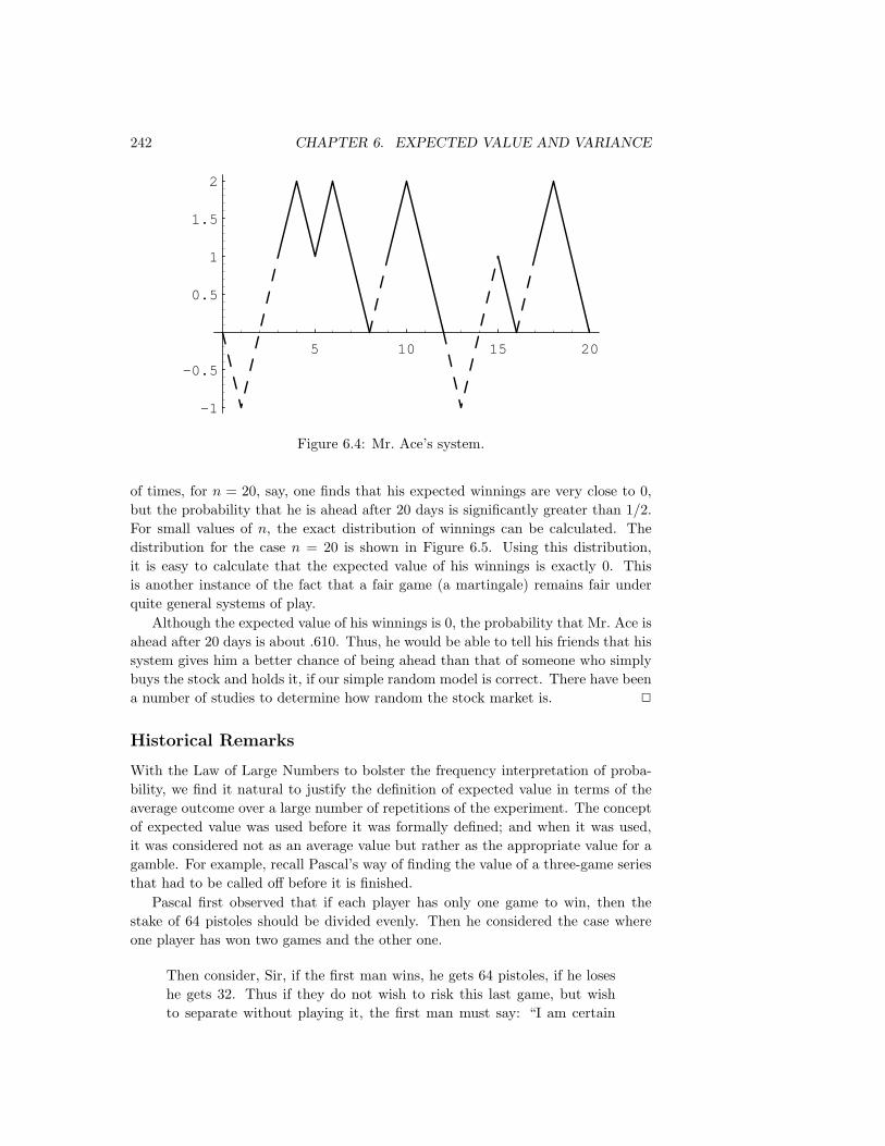
242 CHAPTER 6. EXPECTED VALUE AND VARIANCE
5 10 15 20
-1
-0.5
0.5
1
1.5
2
Figure 6.4: Mr. Ace’s system.
of times, for n = 20, say, one finds that his expected winnings are very close to 0,but the probability that he is ahead after 20 days is significantly greater than 1/2.For small values of n, the exact distribution of winnings can be calculated. Thedistribution for the case n = 20 is shown in Figure 6.5. Using this distribution,it is easy to calculate that the expected value of his winnings is exactly 0. Thisis another instance of the fact that a fair game (a martingale) remains fair underquite general systems of play.
Although the expected value of his winnings is 0, the probability that Mr. Ace isahead after 20 days is about .610. Thus, he would be able to tell his friends that hissystem gives him a better chance of being ahead than that of someone who simplybuys the stock and holds it, if our simple random model is correct. There have beena number of studies to determine how random the stock market is. 2
Historical Remarks
With the Law of Large Numbers to bolster the frequency interpretation of proba-bility, we find it natural to justify the definition of expected value in terms of theaverage outcome over a large number of repetitions of the experiment. The conceptof expected value was used before it was formally defined; and when it was used,it was considered not as an average value but rather as the appropriate value for agamble. For example, recall Pascal’s way of finding the value of a three-game seriesthat had to be called off before it is finished.
Pascal first observed that if each player has only one game to win, then thestake of 64 pistoles should be divided evenly. Then he considered the case whereone player has won two games and the other one.
Then consider, Sir, if the first man wins, he gets 64 pistoles, if he loseshe gets 32. Thus if they do not wish to risk this last game, but wishto separate without playing it, the first man must say: “I am certain
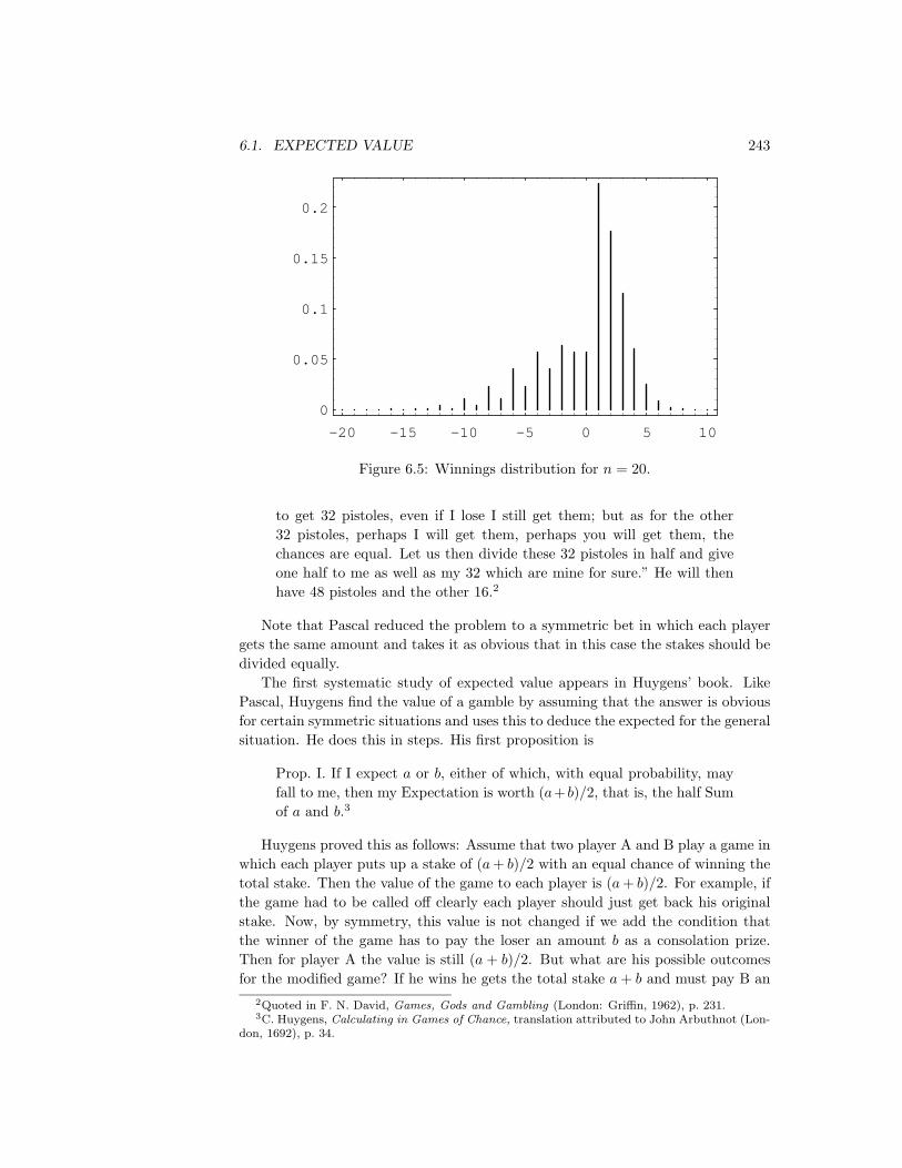
6.1. EXPECTED VALUE 243
-20 -15 -10 -5 0 5 10
0
0.05
0.1
0.15
0.2
Figure 6.5: Winnings distribution for n = 20.
to get 32 pistoles, even if I lose I still get them; but as for the other32 pistoles, perhaps I will get them, perhaps you will get them, thechances are equal. Let us then divide these 32 pistoles in half and giveone half to me as well as my 32 which are mine for sure.” He will thenhave 48 pistoles and the other 16.2
Note that Pascal reduced the problem to a symmetric bet in which each playergets the same amount and takes it as obvious that in this case the stakes should bedivided equally.
The first systematic study of expected value appears in Huygens’ book. LikePascal, Huygens find the value of a gamble by assuming that the answer is obviousfor certain symmetric situations and uses this to deduce the expected for the generalsituation. He does this in steps. His first proposition is
Prop. I. If I expect a or b, either of which, with equal probability, mayfall to me, then my Expectation is worth (a+ b)/2, that is, the half Sumof a and b.3
Huygens proved this as follows: Assume that two player A and B play a game inwhich each player puts up a stake of (a+ b)/2 with an equal chance of winning thetotal stake. Then the value of the game to each player is (a+ b)/2. For example, ifthe game had to be called off clearly each player should just get back his originalstake. Now, by symmetry, this value is not changed if we add the condition thatthe winner of the game has to pay the loser an amount b as a consolation prize.Then for player A the value is still (a + b)/2. But what are his possible outcomesfor the modified game? If he wins he gets the total stake a+ b and must pay B an
2Quoted in F. N. David, Games, Gods and Gambling (London: Griffin, 1962), p. 231.3C. Huygens, Calculating in Games of Chance, translation attributed to John Arbuthnot (Lon-
don, 1692), p. 34.

244 CHAPTER 6. EXPECTED VALUE AND VARIANCE
amount b so ends up with a. If he loses he gets an amount b from player B. Thusplayer A wins a or b with equal chances and the value to him is (a+ b)/2.
Huygens illustrated this proof in terms of an example. If you are offered a gamein which you have an equal chance of winning 2 or 8, the expected value is 5, sincethis game is equivalent to the game in which each player stakes 5 and agrees to paythe loser 3 — a game in which the value is obviously 5.
Huygens’ second proposition is
Prop. II. If I expect a, b, or c, either of which, with equal facility, mayhappen, then the Value of my Expectation is (a+ b+ c)/3, or the thirdof the Sum of a, b, and c.4
His argument here is similar. Three players, A, B, and C, each stake
(a+ b+ c)/3
in a game they have an equal chance of winning. The value of this game to playerA is clearly the amount he has staked. Further, this value is not changed if A entersinto an agreement with B that if one of them wins he pays the other a consolationprize of b and with C that if one of them wins he pays the other a consolation prizeof c. By symmetry these agreements do not change the value of the game. In thismodified game, if A wins he wins the total stake a + b + c minus the consolationprizes b + c giving him a final winning of a. If B wins, A wins b and if C wins, Awins c. Thus A finds himself in a game with value (a+ b+ c)/3 and with outcomesa, b, and c occurring with equal chance. This proves Proposition II.
More generally, this reasoning shows that if there are n outcomes
a1, a2, . . . , an ,
all occurring with the same probability, the expected value is
a1 + a2 + · · ·+ ann
.
In his third proposition Huygens considered the case where you win a or b butwith unequal probabilities. He assumed there are p chances of winning a, and q
chances of winning b, all having the same probability. He then showed that theexpected value is
E =p
p+ q· a+
q
p+ q· b .
This follows by considering an equivalent gamble with p+ q outcomes all occurringwith the same probability and with a payoff of a in p of the outcomes and b in q ofthe outcomes. This allowed Huygens to compute the expected value for experimentswith unequal probabilities, at least when these probablities are rational numbers.
Thus, instead of defining the expected value as a weighted average, Huygensassumed that the expected value of certain symmetric gambles are known and de-duced the other values from these. Although this requires a good deal of clever
4ibid., p. 35.

6.1. EXPECTED VALUE 245
manipulation, Huygens ended up with values that agree with those given by ourmodern definition of expected value. One advantage of this method is that it givesa justification for the expected value in cases where it is not reasonable to assumethat you can repeat the experiment a large number of times, as for example, inbetting that at least two presidents died on the same day of the year. (In fact,three did; all were signers of the Declaration of Independence, and all three died onJuly 4.)
In his book, Huygens calculated the expected value of games using techniquessimilar to those which we used in computing the expected value for roulette atMonte Carlo. For example, his proposition XIV is:
Prop. XIV. If I were playing with another by turns, with two Dice, onthis Condition, that if I throw 7 I gain, and if he throws 6 he gainsallowing him the first Throw: To find the proportion of my Hazard tohis.5
A modern description of this game is as follows. Huygens and his opponent taketurns rolling a die. The game is over if Huygens rolls a 7 or his opponent rolls a 6.His opponent rolls first. What is the probability that Huygens wins the game?
To solve this problem Huygens let x be his chance of winning when his opponentthrew first and y his chance of winning when he threw first. Then on the first rollhis opponent wins on 5 out of the 36 possibilities. Thus,
x =3136· y .
But when Huygens rolls he wins on 6 out of the 36 possible outcomes, and in theother 30, he is led back to where his chances are x. Thus
y =636
+3036· x .
From these two equations Huygens found that x = 31/61.Another early use of expected value appeared in Pascal’s argument to show that
a rational person should believe in the existence of God.6 Pascal said that we haveto make a wager whether to believe or not to believe. Let p denote the probabilitythat God does not exist. His discussion suggests that we are playing a game withtwo strategies, believe and not believe, with payoffs as shown in Table 6.4.
Here −u represents the cost to you of passing up some worldly pleasures asa consequence of believing that God exists. If you do not believe, and God is avengeful God, you will lose x. If God exists and you do believe you will gain v.Now to determine which strategy is best you should compare the two expectedvalues
p(−u) + (1− p)v and p0 + (1− p)(−x),
5ibid., p. 47.6Quoted in I. Hacking, The Emergence of Probability (Cambridge: Cambridge Univ. Press,
1975).

246 CHAPTER 6. EXPECTED VALUE AND VARIANCE
God does not exist God exists
p 1− p
believe −u vnot believe 0 −x
Table 6.4: Payoffs.
Age Survivors0 1006 64
16 4026 2536 1646 1056 666 376 1
Table 6.5: Graunt’s mortality data.
and choose the larger of the two. In general, the choice will depend upon the value ofp. But Pascal assumed that the value of v is infinite and so the strategy of believingis best no matter what probability you assign for the existence of God. This exampleis considered by some to be the beginning of decision theory. Decision analyses ofthis kind appear today in many fields, and, in particular, are an important part ofmedical diagnostics and corporate business decisions.
Another early use of expected value was to decide the price of annuities. Thestudy of statistics has its origins in the use of the bills of mortality kept in theparishes in London from 1603. These records kept a weekly tally of christeningsand burials. From these John Graunt made estimates for the population of Londonand also provided the first mortality data,7 shown in Table 6.5.
As Hacking observes, Graunt apparently constructed this table by assumingthat after the age of 6 there is a constant probability of about 5/8 of survivingfor another decade.8 For example, of the 64 people who survive to age 6, 5/8 of64 or 40 survive to 16, 5/8 of these 40 or 25 survive to 26, and so forth. Of course,he rounded off his figures to the nearest whole person.
Clearly, a constant mortality rate cannot be correct throughout the whole range,and later tables provided by Halley were more realistic in this respect.9
7ibid., p. 108.8ibid., p. 109.9E. Halley, “An Estimate of The Degrees of Mortality of Mankind,” Phil. Trans. Royal. Soc.,

6.1. EXPECTED VALUE 247
A terminal annuity provides a fixed amount of money during a period of n years.To determine the price of a terminal annuity one needs only to know the appropriateinterest rate. A life annuity provides a fixed amount during each year of the buyer’slife. The appropriate price for a life annuity is the expected value of the terminalannuity evaluated for the random lifetime of the buyer. Thus, the work of Huygensin introducing expected value and the work of Graunt and Halley in determiningmortality tables led to a more rational method for pricing annuities. This was oneof the first serious uses of probability theory outside the gambling houses.
Although expected value plays a role now in every branch of science, it retainsits importance in the casino. In 1962, Edward Thorp’s book Beat the Dealer10
provided the reader with a strategy for playing the popular casino game of blackjackthat would assure the player a positive expected winning. This book forevermorechanged the belief of the casinos that they could not be beat.
Exercises
1 A card is drawn at random from a deck consisting of cards numbered 2through 10. A player wins 1 dollar if the number on the card is odd andloses 1 dollar if the number if even. What is the expected value of his win-nings?
2 A card is drawn at random from a deck of playing cards. If it is red, the playerwins 1 dollar; if it is black, the player loses 2 dollars. Find the expected valueof the game.
3 In a class there are 20 students: 3 are 5’ 6”, 5 are 5’8”, 4 are 5’10”, 4 are6’, and 4 are 6’ 2”. A student is chosen at random. What is the student’sexpected height?
4 In Las Vegas the roulette wheel has a 0 and a 00 and then the numbers 1 to 36marked on equal slots; the wheel is spun and a ball stops randomly in oneslot. When a player bets 1 dollar on a number, he receives 36 dollars if theball stops on this number, for a net gain of 35 dollars; otherwise, he loses hisdollar bet. Find the expected value for his winnings.
5 In a second version of roulette in Las Vegas, a player bets on red or black.Half of the numbers from 1 to 36 are red, and half are black. If a player betsa dollar on black, and if the ball stops on a black number, he gets his dollarback and another dollar. If the ball stops on a red number or on 0 or 00 heloses his dollar. Find the expected winnings for this bet.
6 A die is rolled twice. Let X denote the sum of the two numbers that turn up,and Y the difference of the numbers (specifically, the number on the first rollminus the number on the second). Show that E(XY ) = E(X)E(Y ). Are Xand Y independent?
vol. 17 (1693), pp. 596–610; 654–656.10E. Thorp, Beat the Dealer (New York: Random House, 1962).

248 CHAPTER 6. EXPECTED VALUE AND VARIANCE
*7 Show that, if X and Y are random variables taking on only two values each,and if E(XY ) = E(X)E(Y ), then X and Y are independent.
8 A royal family has children until it has a boy or until it has three children,whichever comes first. Assume that each child is a boy with probability 1/2.Find the expected number of boys in this royal family and the expected num-ber of girls.
9 If the first roll in a game of craps is neither a natural nor craps, the playercan make an additional bet, equal to his original one, that he will make hispoint before a seven turns up. If his point is four or ten he is paid off at 2 : 1odds; if it is a five or nine he is paid off at odds 3 : 2; and if it is a six or eighthe is paid off at odds 6 : 5. Find the player’s expected winnings if he makesthis additional bet when he has the opportunity.
10 In Example 6.16 assume that Mr. Ace decides to buy the stock and hold ituntil it goes up 1 dollar and then sell and not buy again. Modify the programStockSystem to find the distribution of his profit under this system aftera twenty-day period. Find the expected profit and the probability that hecomes out ahead.
11 On September 26, 1980, the New York Times reported that a mysteriousstranger strode into a Las Vegas casino, placed a single bet of 777,000 dollarson the “don’t pass” line at the crap table, and walked away with more than1.5 million dollars. In the “don’t pass” bet, the bettor is essentially bettingwith the house. An exception occurs if the roller rolls a 12 on the first roll.In this case, the roller loses and the “don’t pass” better just gets back themoney bet instead of winning. Show that the “don’t pass” bettor has a morefavorable bet than the roller.
12 Recall that in the martingale doubling system (see Exercise 1.1.10), the playerdoubles his bet each time he loses and quits the first time he is ahead. Supposethat you are playing roulette in a fair casino where there are no 0’s, and youbet on red each time. You then win with probability 1/2 each time. Assumethat you start with a 1-dollar bet and employ the martingale system. Sinceyou entered the casino with 100 dollars, you also quit in the unlikely eventthat black turns up six times in a row so that you are down 63 dollars andcannot make the required 64-dollar bet. Find your expected winnings underthis system of play.
13 You have 80 dollars and play the following game. An urn contains two whiteballs and two black balls. You draw the balls out one at a time withoutreplacement until all the balls are gone. On each draw, you bet half of yourpresent fortune that you will draw a white ball. What is your final fortune?
14 In the hat check problem (see Example 3.12), it was assumed that N peoplecheck their hats and the hats are handed back at random. Let Xj = 1 if the

6.1. EXPECTED VALUE 249
jth person gets his or her hat and 0 otherwise. Find E(Xj) and E(Xj ·Xk)for j not equal to k. Are Xj and Xk independent?
15 A box contains two gold balls and three silver balls. You are allowed to choosesuccessively balls from the box at random. You win 1 dollar each time youdraw a gold ball and lose 1 dollar each time you draw a silver ball. After adraw, the ball is not replaced. Show that, if you draw until you are ahead by1 dollar or until there are no more gold balls, this is a favorable game.
16 Gerolamo Cardano in his book, The Gambling Scholar, written in the early1500s, considers the following carnival game. There are six dice. Each of thedice has five blank sides. The sixth side has a number between 1 and 6—adifferent number on each die. The six dice are rolled and the player wins aprize depending on the total of the numbers which turn up.
(a) Find, as Cardano did, the expected total without finding its distribution.
(b) Large prizes were given for large totals with a modest fee to play thegame. Explain why this could be done.
17 Let X be the first time that a failure occurs in an infinite sequence of Bernoullitrials with probability p for success. Let pk = P (X = k) for k = 1, 2, . . . .Show that pk = pk−1q where q = 1 − p. Show that
∑k pk = 1. Show that
E(X) = 1/q. What is the expected number of tosses of a coin required toobtain the first tail?
18 Exactly one of six similar keys opens a certain door. If you try the keys, oneafter another, what is the expected number of keys that you will have to trybefore success?
19 A multiple choice exam is given. A problem has four possible answers, andexactly one answer is correct. The student is allowed to choose a subset ofthe four possible answers as his answer. If his chosen subset contains thecorrect answer, the student receives three points, but he loses one point foreach wrong answer in his chosen subset. Show that if he just guesses a subsetuniformly and randomly his expected score is zero.
20 You are offered the following game to play: a fair coin is tossed until headsturns up for the first time (see Example 6.3). If this occurs on the first tossyou receive 2 dollars, if it occurs on the second toss you receive 22 = 4 dollarsand, in general, if heads turns up for the first time on the nth toss you receive2n dollars.
(a) Show that the expected value of your winnings does not exist (i.e., isgiven by a divergent sum) for this game. Does this mean that this gameis favorable no matter how much you pay to play it?
(b) Assume that you only receive 210 dollars if any number greater than orequal to ten tosses are required to obtain the first head. Show that yourexpected value for this modified game is finite and find its value.

250 CHAPTER 6. EXPECTED VALUE AND VARIANCE
(c) Assume that you pay 10 dollars for each play of the original game. Writea program to simulate 100 plays of the game and see how you do.
(d) Now assume that the utility of n dollars is√n. Write an expression for
the expected utility of the payment, and show that this expression has afinite value. Estimate this value. Repeat this exercise for the case thatthe utility function is log(n).
21 Let X be a random variable which is Poisson distributed with parameter λ.Show that E(X) = λ. Hint : Recall that
ex = 1 + x+x2
2!+x3
3!+ · · · .
22 Recall that in Exercise 1.1.14, we considered a town with two hospitals. Inthe large hospital about 45 babies are born each day, and in the smallerhospital about 15 babies are born each day. We were interested in guessingwhich hospital would have on the average the largest number of days withthe property that more than 60 percent of the children born on that day areboys. For each hospital find the expected number of days in a year that havethe property that more than 60 percent of the children born on that day wereboys.
23 An insurance company has 1,000 policies on men of age 50. The companyestimates that the probability that a man of age 50 dies within a year is .01.Estimate the number of claims that the company can expect from beneficiariesof these men within a year.
24 Using the life table for 1981 in Appendix C, write a program to compute theexpected lifetime for males and females of each possible age from 1 to 85.Compare the results for males and females. Comment on whether life insur-ance should be priced differently for males and females.
*25 A deck of ESP cards consists of 20 cards each of two types: say ten stars,ten circles (normally there are five types). The deck is shuffled and the cardsturned up one at a time. You, the alleged percipient, are to name the symbolon each card before it is turned up.
Suppose that you are really just guessing at the cards. If you do not get tosee each card after you have made your guess, then it is easy to calculate theexpected number of correct guesses, namely ten.
If, on the other hand, you are guessing with information, that is, if you seeeach card after your guess, then, of course, you might expect to get a higherscore. This is indeed the case, but calculating the correct expectation is nolonger easy.
But it is easy to do a computer simulation of this guessing with information,so we can get a good idea of the expectation by simulation. (This is similar tothe way that skilled blackjack players make blackjack into a favorable gameby observing the cards that have already been played. See Exercise 29.)

6.1. EXPECTED VALUE 251
(a) First, do a simulation of guessing without information, repeating theexperiment at least 1000 times. Estimate the expected number of correctanswers and compare your result with the theoretical expectation.
(b) What is the best strategy for guessing with information?
(c) Do a simulation of guessing with information, using the strategy in (b).Repeat the experiment at least 1000 times, and estimate the expectationin this case.
(d) Let S be the number of stars and C the number of circles in the deck. Leth(S,C) be the expected winnings using the optimal guessing strategy in(b). Show that h(S,C) satisfies the recursion relation
h(S,C) =S
S + Ch(S − 1, C) +
C
S + Ch(S,C − 1) +
max(S,C)S + C
,
and h(0, 0) = h(−1, 0) = h(0,−1) = 0. Using this relation, write aprogram to compute h(S,C) and find h(10, 10). Compare the computedvalue of h(10, 10) with the result of your simulation in (c). For moreabout this exercise and Exercise 26 see Diaconis and Graham.11
*26 Consider the ESP problem as described in Exercise 25. You are again guessingwith information, and you are using the optimal guessing strategy of guessingstar if the remaining deck has more stars, circle if more circles, and tossing acoin if the number of stars and circles are equal. Assume that S ≥ C, whereS is the number of stars and C the number of circles.
We can plot the results of a typical game on a graph, where the horizontal axisrepresents the number of steps and the vertical axis represents the differencebetween the number of stars and the number of circles that have been turnedup. A typical game is shown in Figure 6.6. In this particular game, the orderin which the cards were turned up is (C, S, S, S, S, C,C, S, S, C). Thus, in thisparticular game, there were six stars and four circles in the deck. This means,in particular, that every game played with this deck would have a graph whichends at the point (10, 2). We define the line L to be the horizontal line whichgoes through the ending point on the graph (so its vertical coordinate is justthe difference between the number of stars and circles in the deck).
(a) Show that, when the random walk is below the line L, the player guessesright when the graph goes up (star is turned up) and, when the walk isabove the line, the player guesses right when the walk goes down (circleturned up). Show from this property that the subject is sure to have atleast S correct guesses.
(b) When the walk is at a point (x, x) on the line L the number of stars andcircles remaining is the same, and so the subject tosses a coin. Show that
11P. Diaconis and R. Graham, “The Analysis of Sequential Experiments with Feedback to Sub-jects,” Annals of Statistics, vol. 9 (1981), pp. 3–23.
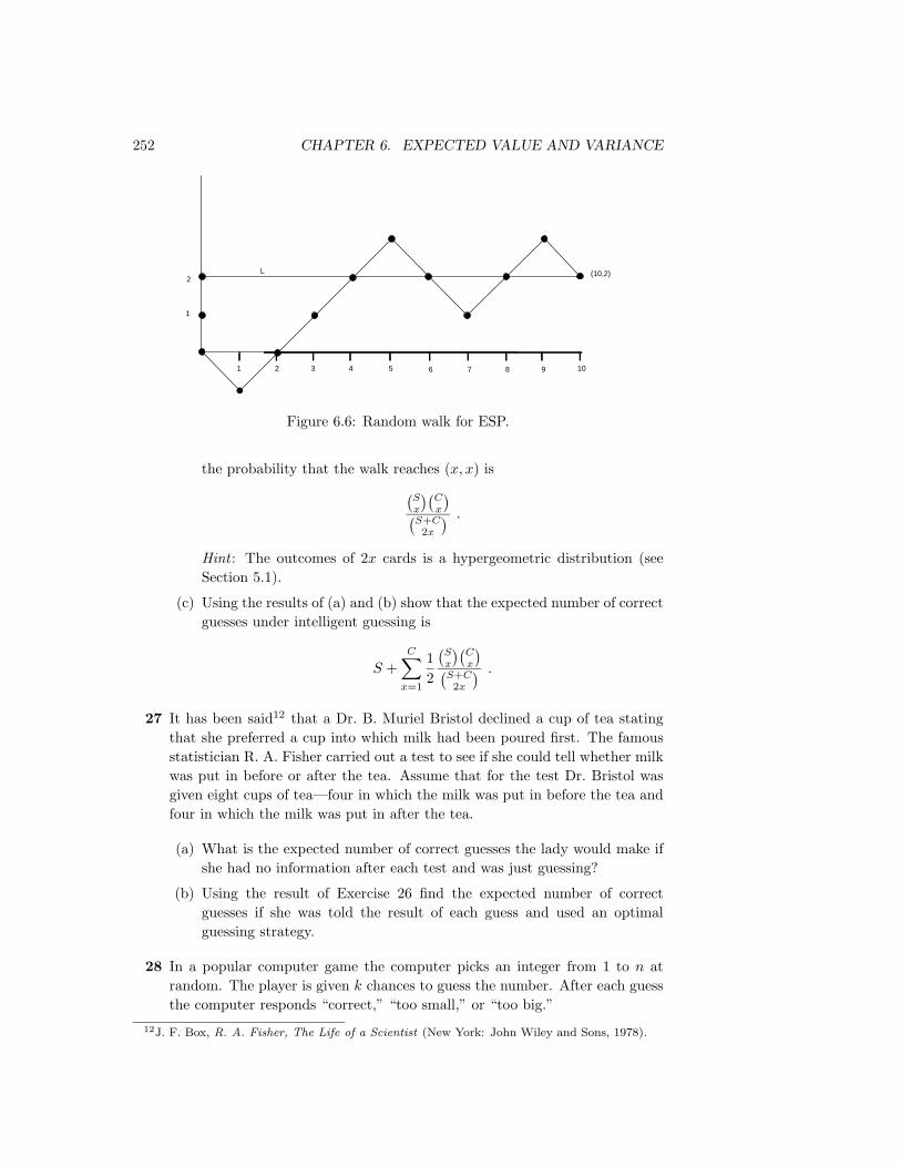
252 CHAPTER 6. EXPECTED VALUE AND VARIANCE
2
1
1 2 3 4 5 6 7 8 9 10
(10,2)L
Figure 6.6: Random walk for ESP.
the probability that the walk reaches (x, x) is(Sx
)(Cx
)(S+C
2x
) .
Hint : The outcomes of 2x cards is a hypergeometric distribution (seeSection 5.1).
(c) Using the results of (a) and (b) show that the expected number of correctguesses under intelligent guessing is
S +C∑x=1
12
(Sx
)(Cx
)(S+C
2x
) .
27 It has been said12 that a Dr. B. Muriel Bristol declined a cup of tea statingthat she preferred a cup into which milk had been poured first. The famousstatistician R. A. Fisher carried out a test to see if she could tell whether milkwas put in before or after the tea. Assume that for the test Dr. Bristol wasgiven eight cups of tea—four in which the milk was put in before the tea andfour in which the milk was put in after the tea.
(a) What is the expected number of correct guesses the lady would make ifshe had no information after each test and was just guessing?
(b) Using the result of Exercise 26 find the expected number of correctguesses if she was told the result of each guess and used an optimalguessing strategy.
28 In a popular computer game the computer picks an integer from 1 to n atrandom. The player is given k chances to guess the number. After each guessthe computer responds “correct,” “too small,” or “too big.”
12J. F. Box, R. A. Fisher, The Life of a Scientist (New York: John Wiley and Sons, 1978).

6.1. EXPECTED VALUE 253
(a) Show that if n ≤ 2k−1, then there is a strategy that guarantees you willcorrectly guess the number in k tries.
(b) Show that if n ≥ 2k−1, there is a strategy that assures you of identifyingone of 2k − 1 numbers and hence gives a probability of (2k − 1)/n ofwinning. Why is this an optimal strategy? Illustrate your result interms of the case n = 9 and k = 3.
29 In the casino game of blackjack the dealer is dealt two cards, one face up andone face down, and each player is dealt two cards, both face down. If thedealer is showing an ace the player can look at his down cards and then makea bet called an insurance bet. (Expert players will recognize why it is calledinsurance.) If you make this bet you will win the bet if the dealer’s secondcard is a ten card : namely, a ten, jack, queen, or king. If you win, you arepaid twice your insurance bet; otherwise you lose this bet. Show that, if theonly cards you can see are the dealer’s ace and your two cards and if yourcards are not ten cards, then the insurance bet is an unfavorable bet. Show,however, that if you are playing two hands simultaneously, and you have noten cards, then it is a favorable bet. (Thorp13 has shown that the game ofblackjack is favorable to the player if he or she can keep good enough trackof the cards that have been played.)
30 Assume that, every time you buy a box of Wheaties, you receive a picture ofone of the n players for the New York Yankees (see Exercise 3.2.34). Let Xk
be the number of additional boxes you have to buy, after you have obtainedk−1 different pictures, in order to obtain the next new picture. Thus X1 = 1,X2 is the number of boxes bought after this to obtain a picture different fromthe first pictured obtained, and so forth.
(a) Show that Xk has a geometric distribution with p = (n− k + 1)/n.
(b) Simulate the experiment for a team with 26 players (25 would be moreaccurate but we want an even number). Carry out a number of simula-tions and estimate the expected time required to get the first 13 playersand the expected time to get the second 13. How do these expectationscompare?
(c) Show that, if there are 2n players, the expected time to get the first halfof the players is
2n(
12n
+1
2n− 1+ · · ·+ 1
n+ 1
),
and the expected time to get the second half is
2n(
1n
+1
n− 1+ · · ·+ 1
).
13E. Thorp, Beat the Dealer (New York: Random House, 1962).

254 CHAPTER 6. EXPECTED VALUE AND VARIANCE
(d) In Section 3.1 we showed that
1 +12
+13
+ · · ·+ 1n∼ logn+ .5772 +
12n
.
Use this to estimate the expression in (c). Compare these estimates withthe exact values and also with your estimates obtained by simulation forthe case n = 26.
*31 (Feller14) A large number, N , of people are subjected to a blood test. Thiscan be administered in two ways: (1) Each person can be tested separately,in this case N test are required, (2) the blood samples of k persons can bepooled and analyzed together. If this test is negative, this one test sufficesfor the k people. If the test is positive, each of the k persons must be testedseparately, and in all, k + 1 tests are required for the k people. Assume thatthe probability p that a test is positive is the same for all people and thatthese events are independent.
(a) Find the probability that the test for a pooled sample of k people willbe positive.
(b) What is the expected value of the number X of tests necessary underplan (2)? (Assume that N is divisible by k.)
(c) For small p, show that the value of k which will minimize the expectednumber of tests under the second plan is approximately 1/
√p.
32 Write a program to add random numbers chosen from [0, 1] until the firsttime the sum is greater than one. Have your program repeat this experimenta number of times to estimate the expected number of selections necessaryin order that the sum of the chosen numbers first exceeds 1. On the basis ofyour experiments, what is your estimate for this number?
*33 The following related discrete problem also gives a good clue for the answerto Exercise 32. Randomly select with replacement t1, t2, . . . , tr from the set(1/n, 2/n, . . . , n/n). Let X be the smallest value of r satisfying
t1 + t2 + · · ·+ tr > 1 .
Then E(X) = (1 + 1/n)n. To prove this, we can just as well choose t1, t2,. . . , tr randomly with replacement from the set (1, 2, . . . , n) and let X be thesmallest value of r for which
t1 + t2 + · · ·+ tr > n .
(a) Use Exercise 3.2.36 to show that
P (X ≥ j + 1) =(n
j
)( 1n
)j.
14W. Feller, Introduction to Probability Theory and Its Applications, 3rd ed., vol. 1 (New York:John Wiley and Sons, 1968), p. 240.

6.1. EXPECTED VALUE 255
(b) Show that
E(X) =n∑j=0
P (X ≥ j + 1) .
(c) From these two facts, find an expression for E(X). This proof is due toHarris Schultz.15
*34 (Banach’s Matchbox16) A man carries in each of his two front pockets a boxof matches originally containing N matches. Whenever he needs a match,he chooses a pocket at random and removes one from that box. One day hereaches into a pocket and finds the box empty.
(a) Let pr denote the probability that the other pocket contains r matches.Define a sequence of counter random variables as follows: Let Xi = 1 ifthe ith draw is from the left pocket, and 0 if it is from the right pocket.Interpret pr in terms of Sn = X1 + X2 + · · · + Xn. Find a binomialexpression for pr.
(b) Write a computer program to compute the pr, as well as the probabilitythat the other pocket contains at least r matches, for N = 100 and r
from 0 to 50.
(c) Show that (N − r)pr = (1/2)(2N + 1)pr+1 − (1/2)(r + 1)pr+1 .
(d) Evaluate∑r pr.
(e) Use (c) and (d) to determine the expectation E of the distribution pr.(f) Use Stirling’s formula to obtain an approximation for E. How many
matches must each box contain to ensure a value of about 13 for theexpectation E? (Take π = 22/7.)
35 A coin is tossed until the first time a head turns up. If this occurs on the nthtoss and n is odd you win 2n/n, but if n is even then you lose 2n/n. Then ifyour expected winnings exist they are given by the convergent series
1− 12
+13− 1
4+ · · ·
called the alternating harmonic series. It is tempting to say that this shouldbe the expected value of the experiment. Show that if we were to do this, theexpected value of an experiment would depend upon the order in which theoutcomes are listed.
36 Suppose we have an urn containing c yellow balls and d green balls. We drawk balls, without replacement, from the urn. Find the expected number ofyellow balls drawn. Hint : Write the number of yellow balls drawn as the sumof c random variables.
15H. Schultz, “An Expected Value Problem,” Two-Year Mathematics Journal, vol. 10, no. 4(1979), pp. 277–78.
16W. Feller, Introduction to Probability Theory, vol. 1, p. 166.

256 CHAPTER 6. EXPECTED VALUE AND VARIANCE
37 The reader is referred to Example 6.13 for an explanation of the various op-tions available in Monte Carlo roulette.
(a) Compute the expected winnings of a 1 franc bet on red under option (a).
(b) Repeat part (a) for option (b).
(c) Compare the expected winnings for all three options.
*38 (from Pittel17) Telephone books, n in number, are kept in a stack. Theprobability that the book numbered i (where 1 ≤ i ≤ n) is consulted for agiven phone call is pi > 0, where the pi’s sum to 1. After a book is used,it is placed at the top of the stack. Assume that the calls are independentand evenly spaced, and that the system has been employed indefinitely farinto the past. Let di be the average depth of book i in the stack. Show thatdi ≤ dj whenever pi ≥ pj . Thus, on the average, the more popular bookshave a tendency to be closer to the top of the stack. Hint : Let pij denote theprobability that book i is above book j. Show that pij = pij(1− pj) + pjipi.
*39 (from Propp18) In the previous problem, let P be the probability that at thepresent time, each book is in its proper place, i.e., book i is ith from the top.Find a formula for P in terms of the pi’s. In addition, find the least upperbound on P , if the pi’s are allowed to vary. Hint : First find the probabilitythat book 1 is in the right place. Then find the probability that book 2 is inthe right place, given that book 1 is in the right place. Continue.
*40 (from H. Shultz and B. Leonard19) A sequence of random numbers in [0, 1)is generated until the sequence is no longer monotone increasing. The num-bers are chosen according to the uniform distribution. What is the expectedlength of the sequence? (In calculating the length, the term that destroysmonotonicity is included.) Hint : Let a1, a2, . . . be the sequence and let Xdenote the length of the sequence. Then
P (X > k) = P (a1 < a2 < · · · < ak) ,
and the probability on the right-hand side is easy to calculate. Furthermore,one can show that
E(X) = 1 + P (X > 1) + P (X > 2) + · · · .
41 Let T be the random variable that counts the number of 2-unshuffles per-formed on an n-card deck until all of the labels on the cards are distinct. Thisrandom variable was discussed in Section 3.3. Using Equation 3.4 in thatsection, together with the formula
E(T ) =∞∑s=0
P (T > s)
17B. Pittel, Problem #1195, Mathematics Magazine, vol. 58, no. 3 (May 1985), pg. 183.18J. Propp, Problem #1159, Mathematics Magazine vol. 57, no. 1 (Feb. 1984), pg. 50.19H. Shultz and B. Leonard, “Unexpected Occurrences of the Number e,” Mathematics Magazine
vol. 62, no. 4 (October, 1989), pp. 269-271.

6.2. VARIANCE OF DISCRETE RANDOM VARIABLES 257
that was proved in Exercise 33, show that
E(T ) =∞∑s=0
(1−
(2s
n
)n!2sn
).
Show that for n = 52, this expression is approximately equal to 11.7. (As wasstated in Chapter 3, this means that on the average, almost 12 riffle shuffles ofa 52-card deck are required in order for the process to be considered random.)
6.2 Variance of Discrete Random Variables
The usefulness of the expected value as a prediction for the outcome of an ex-periment is increased when the outcome is not likely to deviate too much from theexpected value. In this section we shall introduce a measure of this deviation, calledthe variance.
Variance
Definition 6.3 LetX be a numerically valued random variable with expected valueµ = E(X). Then the variance of X, denoted by V (X), is
V (X) = E((X − µ)2) .
2
Note that, by Theorem 6.1, V (X) is given by
V (X) =∑x
(x− µ)2m(x) , (6.1)
where m is the distribution function of X.
Standard Deviation
The standard deviation of X, denoted by D(X), is D(X) =√V (X). We often
write σ for D(X) and σ2 for V (X).
Example 6.17 Consider one roll of a die. Let X be the number that turns up. Tofind V (X), we must first find the expected value of X. This is
µ = E(X) = 1(1
6
)+ 2(1
6
)+ 3(1
6
)+ 4(1
6
)+ 5(1
6
)+ 6(1
6
)=
72.
To find the variance of X, we form the new random variable (X − µ)2 andcompute its expectation. We can easily do this using the following table.

258 CHAPTER 6. EXPECTED VALUE AND VARIANCE
x m(x) (x− 7/2)2
1 1/6 25/42 1/6 9/43 1/6 1/44 1/6 1/45 1/6 9/46 1/6 25/4
Table 6.6: Variance calculation.
From this table we find E((X − µ)2) is
V (X) =16
(254
+94
+14
+14
+94
+254
)=
3512
,
and the standard deviation D(X) =√
35/12 ≈ 1.707. 2
Calculation of Variance
We next prove a theorem that gives us a useful alternative form for computing thevariance.
Theorem 6.6 If X is any random variable with E(X) = µ, then
V (X) = E(X2)− µ2 .
Proof. We have
V (X) = E((X − µ)2) = E(X2 − 2µX + µ2)
= E(X2)− 2µE(X) + µ2 = E(X2)− µ2 .
2
Using Theorem 6.6, we can compute the variance of the outcome of a roll of adie by first computing
E(X2) = 1(1
6
)+ 4(1
6
)+ 9(1
6
)+ 16
(16
)+ 25
(16
)+ 36
(16
)=
916,
and,
V (X) = E(X2)− µ2 =916−(7
2
)2
=3512
,
in agreement with the value obtained directly from the definition of V (X).

6.2. VARIANCE OF DISCRETE RANDOM VARIABLES 259
Properties of Variance
The variance has properties very different from those of the expectation. If c is anyconstant, E(cX) = cE(X) and E(X + c) = E(X) + c. These two statements implythat the expectation is a linear function. However, the variance is not linear, asseen in the next theorem.
Theorem 6.7 If X is any random variable and c is any constant, then
V (cX) = c2V (X)
andV (X + c) = V (X) .
Proof. Let µ = E(X). Then E(cX) = cµ, and
V (cX) = E((cX − cµ)2) = E(c2(X − µ)2)
= c2E((X − µ)2) = c2V (X) .
To prove the second assertion, we note that, to compute V (X + c), we wouldreplace ω by ω+ c and µ by µ+ c in Equation 6.1. But the c’s would cancel, leavingV (X). 2
We turn now to some general properties of the variance. Recall that if X and Yare any two random variables, E(X+Y ) = E(X)+E(Y ). This is not always true forthe case of the variance. For example, let X be a random variable with V (X) 6= 0,and define Y = −X. Then V (X) = V (Y ), so that V (X) + V (Y ) = 2V (X). ButX + Y is always 0 and hence has variance 0. Thus V (X + Y ) 6= V (X) + V (Y ).
In the important case of mutually independent random variables, however, thevariance of the sum is the sum of the variances.
Theorem 6.8 Let X and Y be two independent random variables. Then
V (X + Y ) = V (X) + V (Y ) .
Proof. Let E(X) = a and E(Y ) = b. Then
V (X + Y ) = E((X + Y )2)− (a+ b)2
= E(X2) + 2E(XY ) + E(Y 2)− a2 − 2ab− b2 .
Since X and Y are independent, E(XY ) = E(X)E(Y ) = ab. Thus,
V (X + Y ) = E(X2)− a2 + E(Y 2)− b2 = V (X) + V (Y ) .
2

260 CHAPTER 6. EXPECTED VALUE AND VARIANCE
It is easy to extend this proof, by mathematical induction, to show that thevariance of the sum of any number of mutually independent random variables is thesum of the individual variances. Thus we have the following theorem.
Theorem 6.9 Let X1, X2, . . . , Xn be an independent trials process with E(Xj) =µ and V (Xj) = σ2. Let
Sn = X1 +X2 + · · ·+Xn
be the sum, and
An =Snn
be the average. Then
E(Sn) = nµ ,
V (Sn) = nσ2 ,
E(An) = µ ,
V (An) =σ2
n.
Proof. Since all the random variables Xj have the same expected value, we have
E(Sn) = E(X1) + · · ·+ E(Xn) = nµ ,
andV (Sn) = V (X1) + · · ·+ V (Xn) = nσ2 .
We have seen that, if we multiply a random variable X with mean µ and varianceσ2 by a constant c, the new random variable has expected value cµ and variancec2σ2. Thus,
E(An) = E
(Snn
)=nµ
n= µ ,
and
V (An) = V
(Snn
)=V (Sn)n2
=nσ2
n2=σ2
n.
Finally, the standard deviation of An is given by
σ(An) =σ√n.
2
The last statement in the above proof implies that in an independent trials pro-cess, if the individual summands have finite variance, then the standard deviationof the average goes to 0 as n→∞. Since the standard deviation tells us somethingabout the spread of the distribution around the mean, we see that for large values ofn, the value of An is usually very close to the mean of An, which equals µ, as shownabove. This statement is made precise in Chapter 8, where it is called the Law ofLarge Numbers. For example, let X represent the roll of a fair die. In Figure 6.7,we show the distribution of a random variable An corresponding to X, for n = 10and n = 100.

6.2. VARIANCE OF DISCRETE RANDOM VARIABLES 261
1 2 3 4 5 60
0.1
0.2
0.3
0.4
0.5
0.6
2 2.5 3 3.5 4 4.5 50
0.5
1
1.5
2n = 10 n = 100
Figure 6.7: Empirical distribution of An.
Example 6.18 Consider n rolls of a die. We have seen that, if Xj is the outcomeif the jth roll, then E(Xj) = 7/2 and V (Xj) = 35/12. Thus, if Sn is the sum of theoutcomes, and An = Sn/n is the average of the outcomes, we have E(An) = 7/2 andV (An) = (35/12)/n. Therefore, as n increases, the expected value of the averageremains constant, but the variance tends to 0. If the variance is a measure of theexpected deviation from the mean this would indicate that, for large n, we canexpect the average to be very near the expected value. This is in fact the case, andwe shall justify it in Chapter 8. 2
Bernoulli Trials
Consider next the general Bernoulli trials process. As usual, we let Xj = 1 if thejth outcome is a success and 0 if it is a failure. If p is the probability of a success,and q = 1− p, then
E(Xj) = 0q + 1p = p ,
E(X2j ) = 02q + 12p = p ,
andV (Xj) = E(X2
j )− (E(Xj))2 = p− p2 = pq .
Thus, for Bernoulli trials, if Sn = X1 +X2 + · · ·+Xn is the number of successes,then E(Sn) = np, V (Sn) = npq, and D(Sn) =
√npq. If An = Sn/n is the average
number of successes, then E(An) = p, V (An) = pq/n, and D(An) =√pq/n. We
see that the expected proportion of successes remains p and the variance tends to 0.This suggests that the frequency interpretation of probability is a correct one. Weshall make this more precise in Chapter 8.
Example 6.19 Let T denote the number of trials until the first success in aBernoulli trials process. Then T is geometrically distributed. What is the vari-ance of T? In Example 4.15, we saw that
mT =(
1 2 3 · · ·p qp q2p · · ·
).

262 CHAPTER 6. EXPECTED VALUE AND VARIANCE
In Example 6.4, we showed that
E(T ) = 1/p .
Thus,V (T ) = E(T 2)− 1/p2 ,
so we need only find
E(T 2) = 1p+ 4qp+ 9q2p+ · · ·= p(1 + 4q + 9q2 + · · ·) .
To evaluate this sum, we start again with
1 + x+ x2 + · · · = 11− x .
Differentiating, we obtain
1 + 2x+ 3x2 + · · · = 1(1− x)2
.
Multiplying by x,x+ 2x2 + 3x3 + · · · = x
(1− x)2.
Differentiating again gives
1 + 4x+ 9x2 + · · · = 1 + x
(1− x)3.
Thus,
E(T 2) = p1 + q
(1− q)3=
1 + q
p2
and
V (T ) = E(T 2)− (E(T ))2
=1 + q
p2− 1p2
=q
p2.
For example, the variance for the number of tosses of a coin until the firsthead turns up is (1/2)/(1/2)2 = 2. The variance for the number of rolls of adie until the first six turns up is (5/6)/(1/6)2 = 30. Note that, as p decreases, thevariance increases rapidly. This corresponds to the increased spread of the geometricdistribution as p decreases (noted in Figure 5.1). 2
Poisson Distribution
Just as in the case of expected values, it is easy to guess the variance of the Poissondistribution with parameter λ. We recall that the variance of a binomial distributionwith parameters n and p equals npq. We also recall that the Poisson distributioncould be obtained as a limit of binomial distributions, if n goes to ∞ and p goesto 0 in such a way that their product is kept fixed at the value λ. In this case,npq = λq approaches λ, since q goes to 1. So, given a Poisson distribution withparameter λ, we should guess that its variance is λ. The reader is asked to showthis in Exercise 29.

6.2. VARIANCE OF DISCRETE RANDOM VARIABLES 263
Exercises
1 A number is chosen at random from the set S = −1, 0, 1. Let X be thenumber chosen. Find the expected value, variance, and standard deviation ofX.
2 A random variable X has the distribution
pX =(
0 1 2 41/3 1/3 1/6 1/6
).
Find the expected value, variance, and standard deviation of X.
3 You place a 1-dollar bet on the number 17 at Las Vegas, and your friendplaces a 1-dollar bet on black (see Exercises 1.1.6 and 1.1.7). Let X be yourwinnings and Y be her winnings. Compare E(X), E(Y ), and V (X), V (Y ).What do these computations tell you about the nature of your winnings ifyou and your friend make a sequence of bets, with you betting each time ona number and your friend betting on a color?
4 X is a random variable with E(X) = 100 and V (X) = 15. Find
(a) E(X2).
(b) E(3X + 10).
(c) E(−X).
(d) V (−X).
(e) D(−X).
5 In a certain manufacturing process, the (Fahrenheit) temperature never variesby more than 2 from 62. The temperature is, in fact, a random variable Fwith distribution
PF =(
60 61 62 63 641/10 2/10 4/10 2/10 1/10
).
(a) Find E(F ) and V (F ).
(b) Define T = F − 62. Find E(T ) and V (T ), and compare these answerswith those in part (a).
(c) It is decided to report the temperature readings on a Celsius scale, thatis, C = (5/9)(F − 32). What is the expected value and variance for thereadings now?
6 Write a computer program to calculate the mean and variance of a distributionwhich you specify as data. Use the program to compare the variances for thefollowing densities, both having expected value 0:
pX =(−2 −1 0 1 2
3/11 2/11 1/11 2/11 3/11
);
pY =(−2 −1 0 1 2
1/11 2/11 5/11 2/11 1/11
).

264 CHAPTER 6. EXPECTED VALUE AND VARIANCE
7 A coin is tossed three times. Let X be the number of heads that turn up.Find V (X) and D(X).
8 A random sample of 2400 people are asked if they favor a government pro-posal to develop new nuclear power plants. If 40 percent of the people in thecountry are in favor of this proposal, find the expected value and the stan-dard deviation for the number S2400 of people in the sample who favored theproposal.
9 A die is loaded so that the probability of a face coming up is proportional tothe number on that face. The die is rolled with outcome X. Find V (X) andD(X).
10 Prove the following facts about the standard deviation.
(a) D(X + c) = D(X).
(b) D(cX) = |c|D(X).
11 A number is chosen at random from the integers 1, 2, 3, . . . , n. Let X be thenumber chosen. Show that E(X) = (n+ 1)/2 and V (X) = (n− 1)(n+ 1)/12.Hint : The following identity may be useful:
12 + 22 + · · ·+ n2 =(n)(n+ 1)(2n+ 1)
6.
12 Let X be a random variable with µ = E(X) and σ2 = V (X). Define X∗ =(X−µ)/σ. The random variable X∗ is called the standardized random variableassociated with X. Show that this standardized random variable has expectedvalue 0 and variance 1.
13 Peter and Paul play Heads or Tails (see Example 1.4). Let Wn be Peter’swinnings after n matches. Show that E(Wn) = 0 and V (Wn) = n.
14 Find the expected value and the variance for the number of boys and thenumber of girls in a royal family that has children until there is a boy or untilthere are three children, whichever comes first.
15 Suppose that n people have their hats returned at random. Let Xi = 1 if theith person gets his or her own hat back and 0 otherwise. Let Sn =
∑ni=1Xi.
Then Sn is the total number of people who get their own hats back. Showthat
(a) E(X2i ) = 1/n.
(b) E(Xi ·Xj) = 1/n(n− 1) for i 6= j.
(c) E(S2n) = 2 (using (a) and (b)).
(d) V (Sn) = 1.

6.2. VARIANCE OF DISCRETE RANDOM VARIABLES 265
16 Let Sn be the number of successes in n independent trials. Use the programBinomialProbabilities (Section 3.2) to compute, for given n, p, and j, theprobability
P (−j√npq < Sn − np < j√npq) .
(a) Let p = .5, and compute this probability for j = 1, 2, 3 and n = 10, 30, 50.Do the same for p = .2.
(b) Show that the standardized random variable S∗n = (Sn − np)/√npq has
expected value 0 and variance 1. What do your results from (a) tell youabout this standardized quantity S∗n?
17 Let X be the outcome of a chance experiment with E(X) = µ and V (X) =σ2. When µ and σ2 are unknown, the statistician often estimates them byrepeating the experiment n times with outcomes x1, x2, . . . , xn, estimatingµ by the sample mean
x =1n
n∑i=1
xi ,
and σ2 by the sample variance
s2 =1n
n∑i=1
(xi − x)2 .
Then s is the sample standard deviation. These formulas should remind thereader of the definitions of the theoretical mean and variance. (Many statisti-cians define the sample variance with the coefficient 1/n replaced by 1/(n−1).If this alternative definition is used, the expected value of s2 is equal to σ2.See Exercise 18, part (d).)
Write a computer program that will roll a die n times and compute the samplemean and sample variance. Repeat this experiment several times for n = 10and n = 1000. How well do the sample mean and sample variance estimatethe true mean 7/2 and variance 35/12?
18 Show that, for the sample mean x and sample variance s2 as defined in Exer-cise 17,
(a) E(x) = µ.
(b) E((x− µ)2
)= σ2/n.
(c) E(s2) = n−1n σ2. Hint : For (c) write
n∑i=1
(xi − x)2 =n∑i=1
((xi − µ)− (x− µ)
)2=
n∑i=1
(xi − µ)2 − 2(x− µ)n∑i=1
(xi − µ) + n(x− µ)2
=n∑i=1
(xi − µ)2 − n(x− µ)2,

266 CHAPTER 6. EXPECTED VALUE AND VARIANCE
and take expectations of both sides, using part (b) when necessary.
(d) Show that if, in the definition of s2 in Exercise 17, we replace the coeffi-cient 1/n by the coefficient 1/(n−1), then E(s2) = σ2. (This shows whymany statisticians use the coefficient 1/(n − 1). The number s2 is usedto estimate the unknown quantity σ2. If an estimator has an averagevalue which equals the quantity being estimated, then the estimator issaid to be unbiased . Thus, the statement E(s2) = σ2 says that s2 is anunbiased estimator of σ2.)
19 Let X be a random variable taking on values a1, a2, . . . , ar with probabilitiesp1, p2, . . . , pr and with E(X) = µ. Define the spread of X as follows:
σ =r∑i=1
|ai − µ|pi .
This, like the standard deviation, is a way to quantify the amount that arandom variable is spread out around its mean. Recall that the variance of asum of mutually independent random variables is the sum of the individualvariances. The square of the spread corresponds to the variance in a mannersimilar to the correspondence between the spread and the standard deviation.Show by an example that it is not necessarily true that the square of thespread of the sum of two independent random variables is the sum of thesquares of the individual spreads.
20 We have two instruments that measure the distance between two points. Themeasurements given by the two instruments are random variables X1 andX2 that are independent with E(X1) = E(X2) = µ, where µ is the truedistance. From experience with these instruments, we know the values of thevariances σ2
1 and σ22 . These variances are not necessarily the same. From two
measurements, we estimate µ by the weighted average µ = wX1 + (1−w)X2.Here w is chosen in [0, 1] to minimize the variance of µ.
(a) What is E(µ)?
(b) How should w be chosen in [0, 1] to minimize the variance of µ?
21 Let X be a random variable with E(X) = µ and V (X) = σ2. Show that thefunction f(x) defined by
f(x) =∑ω
(X(ω)− x)2p(ω)
has its minimum value when x = µ.
22 Let X and Y be two random variables defined on the finite sample space Ω.Assume that X, Y , X + Y , and X − Y all have the same distribution. Provethat P (X = Y = 0) = 1.

6.2. VARIANCE OF DISCRETE RANDOM VARIABLES 267
23 If X and Y are any two random variables, then the covariance of X and Y isdefined by Cov(X,Y ) = E((X −E(X))(Y −E(Y ))). Note that Cov(X,X) =V (X). Show that, if X and Y are independent, then Cov(X,Y ) = 0; andshow, by an example, that we can have Cov(X,Y ) = 0 and X and Y notindependent.
*24 A professor wishes to make up a true-false exam with n questions. She assumesthat she can design the problems in such a way that a student will answerthe jth problem correctly with probability pj , and that the answers to thevarious problems may be considered independent experiments. Let Sn be thenumber of problems that a student will get correct. The professor wishes tochoose pj so that E(Sn) = .7n and so that the variance of Sn is as large aspossible. Show that, to achieve this, she should choose pj = .7 for all j; thatis, she should make all the problems have the same difficulty.
25 (Lamperti20) An urn contains exactly 5000 balls, of which an unknown numberX are white and the rest red, where X is a random variable with a probabilitydistribution on the integers 0, 1, 2, . . . , 5000.
(a) Suppose we know that E(X) = µ. Show that this is enough to allow usto calculate the probability that a ball drawn at random from the urnwill be white. What is this probability?
(b) We draw a ball from the urn, examine its color, replace it, and thendraw another. Under what conditions, if any, are the results of the twodrawings independent; that is, does
P (white,white) = P (white)2 ?
(c) Suppose the variance of X is σ2. What is the probability of drawing twowhite balls in part (b)?
26 For a sequence of Bernoulli trials, let X1 be the number of trials until the firstsuccess. For j ≥ 2, let Xj be the number of trials after the (j − 1)st successuntil the jth success. It can be shown that X1, X2, . . . is an independent trialsprocess.
(a) What is the common distribution, expected value, and variance for Xj?
(b) Let Tn = X1 +X2 + · · ·+Xn. Then Tn is the time until the nth success.Find E(Tn) and V (Tn).
(c) Use the results of (b) to find the expected value and variance for thenumber of tosses of a coin until the nth occurrence of a head.
27 Referring to Exercise 6.1.30, find the variance for the number of boxes ofWheaties bought before getting half of the players’ pictures and the variancefor the number of additional boxes needed to get the second half of the players’pictures.
20Private communication.

268 CHAPTER 6. EXPECTED VALUE AND VARIANCE
28 In Example 5.3, assume that the book in question has 1000 pages. Let X bethe number of pages with no mistakes. Show that E(X) = 905 and V (X) =86. Using these results, show that the probability is ≤ .05 that there will bemore than 924 pages without errors or fewer than 866 pages without errors.
29 Let X be Poisson distributed with parameter λ. Show that V (X) = λ.
6.3 Continuous Random Variables
In this section we consider the properties of the expected value and the varianceof a continuous random variable. These quantities are defined just as for discreterandom variables and share the same properties.
Expected Value
Definition 6.4 Let X be a real-valued random variable with density function f(x).The expected value µ = E(X) is defined by
µ = E(X) =∫ +∞
−∞xf(x) dx ,
provided the integral ∫ +∞
−∞|x|f(x) dx
is finite. 2
The reader should compare this definition with the corresponding one for discreterandom variables in Section 6.1. Intuitively, we can interpret E(X), as we did inthe previous sections, as the value that we should expect to obtain if we perform alarge number of independent experiments and average the resulting values of X.
We can summarize the properties of E(X) as follows (cf. Theorem 6.2).
Theorem 6.10 If X and Y are real-valued random variables and c is any constant,then
E(X + Y ) = E(X) + E(Y ) ,
E(cX) = cE(X) .
The proof is very similar to the proof of Theorem 6.2, and we omit it. 2
More generally, if X1, X2, . . . , Xn are n real-valued random variables, and c1, c2,. . . , cn are n constants, then
E(c1X1 + c2X2 + · · ·+ cnXn) = c1E(X1) + c2E(X2) + · · ·+ cnE(Xn) .

6.3. CONTINUOUS RANDOM VARIABLES 269
Example 6.20 Let X be uniformly distributed on the interval [0, 1]. Then
E(X) =∫ 1
0
x dx = 1/2 .
It follows that if we choose a large number N of random numbers from [0, 1] and takethe average, then we can expect that this average should be close to the expectedvalue of 1/2. 2
Example 6.21 Let Z = (x, y) denote a point chosen uniformly and randomly fromthe unit disk, as in the dart game in Example 2.8 and let X = (x2 + y2)1/2 be thedistance from Z to the center of the disk. The density function of X can easily beshown to equal f(x) = 2x, so by the definition of expected value,
E(X) =∫ 1
0
xf(x) dx
=∫ 1
0
x(2x) dx
=23.
2
Example 6.22 In the example of the couple meeting at the Inn (Example 2.16),each person arrives at a time which is uniformly distributed between 5:00 and 6:00PM. The random variable Z under consideration is the length of time the firstperson has to wait until the second one arrives. It was shown that
fZ(z) = 2(1− z) ,
for 0 ≤ z ≤ 1. Hence,
E(Z) =∫ 1
0
zfZ(z) dz
=∫ 1
0
2z(1− z) dz
=[z2 − 2
3z3]1
0
=13.
2
Expectation of a Function of a Random Variable
Suppose that X is a real-valued random variable and φ(x) is a continuous functionfrom R to R. The following theorem is the continuous analogue of Theorem 6.1.
270 CHAPTER 6. EXPECTED VALUE AND VARIANCE
Theorem 6.11 If X is a real-valued random variable and if φ : R → R is acontinuous real-valued function with domain [a, b], then
E(φ(X)) =∫ +∞
−∞φ(x)fX(x) dx ,
provided the integral exists. 2
For a proof of this theorem, see Ross.21
Expectation of the Product of Two Random Variables
In general, it is not true that E(XY ) = E(X)E(Y ), since the integral of a product isnot the product of integrals. But if X and Y are independent, then the expectationsmultiply.
Theorem 6.12 Let X and Y be independent real-valued continuous random vari-ables with finite expected values. Then we have
E(XY ) = E(X)E(Y ) .
Proof. We will prove this only in the case that the ranges of X and Y are containedin the intervals [a, b] and [c, d], respectively. Let the density functions of X and Y
be denoted by fX(x) and fY (y), respectively. Since X and Y are independent, thejoint density function of X and Y is the product of the individual density functions.Hence
E(XY ) =∫ b
a
∫ d
c
xyfX(x)fY (y) dy dx
=∫ b
a
xfX(x) dx∫ d
c
yfY (y) dy
= E(X)E(Y ) .
The proof in the general case involves using sequences of bounded random vari-ables that approach X and Y , and is somewhat technical, so we will omit it. 2
In the same way, one can show that if X1, X2, . . . , Xn are n mutually indepen-dent real-valued random variables, then
E(X1X2 · · ·Xn) = E(X1)E(X2) · · · E(Xn) .
Example 6.23 Let Z = (X,Y ) be a point chosen at random in the unit square.Let A = X2 and B = Y 2. Then Theorem 4.3 implies that A and B are independent.Using Theorem 6.11, the expectations of A and B are easy to calculate:
E(A) = E(B) =∫ 1
0
x2 dx
=13.
21S. Ross, A First Course in Probability, (New York: Macmillan, 1984), pgs. 241-245.

6.3. CONTINUOUS RANDOM VARIABLES 271
Using Theorem 6.12, the expectation of AB is just the product of E(A) and E(B),or 1/9. The usefulness of this theorem is demonstrated by noting that it is quite abit more difficult to calculate E(AB) from the definition of expectation. One findsthat the density function of AB is
fAB(t) =− log(t)
4√t
,
so
E(AB) =∫ 1
0
tfAB(t) dt
=19.
2
Example 6.24 Again let Z = (X,Y ) be a point chosen at random in the unitsquare, and let W = X + Y . Then Y and W are not independent, and we have
E(Y ) =12,
E(W ) = 1 ,
E(YW ) = E(XY + Y 2) = E(X)E(Y ) +13
=7126= E(Y )E(W ) .
2
We turn now to the variance.
Variance
Definition 6.5 Let X be a real-valued random variable with density function f(x).The variance σ2 = V (X) is defined by
σ2 = V (X) = E((X − µ)2) .
2
The next result follows easily from Theorem 6.1. There is another way to calculatethe variance of a continuous random variable, which is usually slightly easier. It isgiven in Theorem 6.15.
Theorem 6.13 If X is a real-valued random variable with E(X) = µ, then
σ2 =∫ ∞−∞
(x− µ)2f(x) dx .
2

272 CHAPTER 6. EXPECTED VALUE AND VARIANCE
The properties listed in the next three theorems are all proved in exactly thesame way that the corresponding theorems for discrete random variables wereproved in Section 6.2.
Theorem 6.14 If X is a real-valued random variable defined on Ω and c is anyconstant, then (cf. Theorem 6.7)
V (cX) = c2V (X) ,
V (X + c) = V (X) .
2
Theorem 6.15 If X is a real-valued random variable with E(X) = µ, then (cf.Theorem 6.6)
V (X) = E(X2)− µ2 .
2
Theorem 6.16 If X and Y are independent real-valued random variables on Ω,then (cf. Theorem 6.8)
V (X + Y ) = V (X) + V (Y ) .
2
Example 6.25 (continuation of Example 6.20) If X is uniformly distributed on[0, 1], then, using Theorem 6.15, we have
V (X) =∫ 1
0
(x− 1
2
)2
dx =112
.
2
Example 6.26 Let X be an exponentially distributed random variable with pa-rameter λ. Then the density function of X is
fX(x) = λe−λx .
From the definition of expectation and integration by parts, we have
E(X) =∫ ∞
0
xfX(x) dx
= λ
∫ ∞0
xe−λx dx
= −xe−λx∣∣∣∣∞0
+∫ ∞
0
e−λx dx
= 0 +e−λx
−λ
∣∣∣∣∞0
=1λ.

6.3. CONTINUOUS RANDOM VARIABLES 273
Similarly, using Theorems 6.11 and 6.15, we have
V (X) =∫ ∞
0
x2fX(x) dx− 1λ2
= λ
∫ ∞0
x2e−λx dx− 1λ2
= −x2e−λx∣∣∣∣∞0
+ 2∫ ∞
0
xe−λx dx− 1λ2
= −x2e−λx∣∣∣∣∞0
− 2xe−λx
λ
∣∣∣∣∞0
− 2λ2e−λx
∣∣∣∣∞0
− 1λ2
=2λ2− 1λ2
=1λ2
.
In this case, both E(X) and V (X) are finite if λ > 0. 2
Example 6.27 Let Z be a standard normal random variable with density function
fZ(x) =1√2πe−x
2/2 .
Since this density function is symmetric with respect to the y-axis, then it is easyto show that ∫ ∞
−∞xfZ(x) dx
has value 0. The reader should recall however, that the expectation is defined to bethe above integral only if the integral∫ ∞
−∞|x|fZ(x) dx
is finite. This integral equals
2∫ ∞
0
xfZ(x) dx ,
which one can easily show is finite. Thus, the expected value of Z is 0.To calculate the variance of Z, we begin by applying Theorem 6.15:
V (Z) =∫ +∞
−∞x2fZ(x) dx− µ2 .
If we write x2 as x · x, and integrate by parts, we obtain
1√2π
(−xe−x2/2)∣∣∣∣+∞−∞
+1√2π
∫ +∞
−∞e−x
2/2 dx .
The first summand above can be shown to equal 0, since as x → ±∞, e−x2/2 gets
small more quickly than x gets large. The second summand is just the standardnormal density integrated over its domain, so the value of this summand is 1.Therefore, the variance of the standard normal density equals 1.

274 CHAPTER 6. EXPECTED VALUE AND VARIANCE
Now let X be a (not necessarily standard) normal random variable with param-eters µ and σ. Then the density function of X is
fX(x) =1√2πσ
e−(x−µ)2/2σ2.
We can write X = σZ + µ, where Z is a standard normal random variable. SinceE(Z) = 0 and V (Z) = 1 by the calculation above, Theorems 6.10 and 6.14 implythat
E(X) = E(σZ + µ) = µ ,
V (X) = V (σZ + µ) = σ2 .
2
Example 6.28 Let X be a continuous random variable with the Cauchy densityfunction
fX(x) =a
π
1a2 + x2
.
Then the expectation of X does not exist, because the integral
a
π
∫ +∞
−∞
|x| dxa2 + x2
diverges. Thus the variance of X also fails to exist. Densities whose variance is notdefined, like the Cauchy density, behave quite differently in a number of importantrespects from those whose variance is finite. We shall see one instance of thisdifference in Section 8.2. 2
Independent Trials
Corollary 6.1 If X1, X2, . . . , Xn is an independent trials process of real-valuedrandom variables, with E(Xi) = µ and V (Xi) = σ2, and if
Sn = X1 +X2 + · · ·+Xn ,
An =Snn
,
then
E(Sn) = nµ ,
E(An) = µ ,
V (Sn) = nσ2 ,
V (An) =σ2
n.
It follows that if we setS∗n =
Sn − nµ√nσ2
,

6.3. CONTINUOUS RANDOM VARIABLES 275
then
E(S∗n) = 0 ,
V (S∗n) = 1 .
We say that S∗n is a standardized version of Sn (see Exercise 12 in Section 6.2). 2
Queues
Example 6.29 Let us consider again the queueing problem, that is, the problem ofthe customers waiting in a queue for service (see Example 5.7). We suppose againthat customers join the queue in such a way that the time between arrivals is anexponentially distributed random variable X with density function
fX(t) = λe−λt .
Then the expected value of the time between arrivals is simply 1/λ (see Exam-ple 6.26), as was stated in Example 5.7. The reciprocal λ of this expected valueis often referred to as the arrival rate. The service time of an individual who isfirst in line is defined to be the amount of time that the person stays at the headof the line before leaving. We suppose that the customers are served in such a waythat the service time is another exponentially distributed random variable Y withdensity function
fX(t) = µe−µt .
Then the expected value of the service time is
E(X) =∫ ∞
0
tfX(t) dt =1µ.
The reciprocal µ if this expected value is often referred to as the service rate.We expect on grounds of our everyday experience with queues that if the service
rate is greater than the arrival rate, then the average queue size will tend to stabilize,but if the service rate is less than the arrival rate, then the queue will tend to increasein length without limit (see Figure 5.7). The simulations in Example 5.7 tend tobear out our everyday experience. We can make this conclusion more precise if weintroduce the traffic intensity as the product
ρ = (arrival rate)(average service time) =λ
µ=
1/µ1/λ
.
The traffic intensity is also the ratio of the average service time to the averagetime between arrivals. If the traffic intensity is less than 1 the queue will performreasonably, but if it is greater than 1 the queue will grow indefinitely large. In thecritical case of ρ = 1, it can be shown that the queue will become large but therewill always be times at which the queue is empty.22
22L. Kleinrock, Queueing Systems, vol. 2 (New York: John Wiley and Sons, 1975).

276 CHAPTER 6. EXPECTED VALUE AND VARIANCE
In the case that the traffic intensity is less than 1 we can consider the length ofthe queue as a random variable Z whose expected value is finite,
E(Z) = N .
The time spent in the queue by a single customer can be considered as a randomvariable W whose expected value is finite,
E(W ) = T .
Then we can argue that, when a customer joins the queue, he expects to find N
people ahead of him, and when he leaves the queue, he expects to find λT peoplebehind him. Since, in equilibrium, these should be the same, we would expect tofind that
N = λT .
This last relationship is called Little’s law for queues.23 We will not prove it here.A proof may be found in Ross.24 Note that in this case we are counting the waitingtime of all customers, even those that do not have to wait at all. In our simulationin Section 4.2, we did not consider these customers.
If we knew the expected queue length then we could use Little’s law to obtainthe expected waiting time, since
T =N
λ.
The queue length is a random variable with a discrete distribution. We can estimatethis distribution by simulation, keeping track of the queue lengths at the times atwhich a customer arrives. We show the result of this simulation (using the programQueue) in Figure 6.8.
We note that the distribution appears to be a geometric distribution. In thestudy of queueing theory it is shown that the distribution for the queue length inequilibrium is indeed a geometric distribution with
sj = (1− ρ)ρj for j = 0, 1, 2, . . . ,
if ρ < 1. The expected value of a random variable with this distribution is
N =ρ
(1− ρ)
(see Example 6.4). Thus by Little’s result the expected waiting time is
T =ρ
λ(1− ρ)=
1µ− λ ,
where µ is the service rate, λ the arrival rate, and ρ the traffic intensity.
23ibid., p. 17.24S. M. Ross, Applied Probability Models with Optimization Applications, (San Francisco:
Holden-Day, 1970)

6.3. CONTINUOUS RANDOM VARIABLES 277
0 10 20 30 40 500
0.02
0.04
0.06
0.08
Figure 6.8: Distribution of queue lengths.
In our simulation, the arrival rate is 1 and the service rate is 1.1. Thus, thetraffic intensity is 1/1.1 = 10/11, the expected queue size is
10/11(1− 10/11)
= 10 ,
and the expected waiting time is
11.1− 1
= 10 .
In our simulation the average queue size was 8.19 and the average waiting time was7.37. In Figure 6.9, we show the histogram for the waiting times. This histogramsuggests that the density for the waiting times is exponential with parameter µ−λ,and this is the case. 2
Exercises
1 Let X be a random variable with range [−1, 1] and let fX(x) be the densityfunction of X. Find µ(X) and σ2(X) if, for |x| < 1,
(a) fX(x) = 1/2.
(b) fX(x) = |x|.(c) fX(x) = 1− |x|.(d) fX(x) = (3/2)x2.
2 Let X be a random variable with range [−1, 1] and fX its density function.Find µ(X) and σ2(X) if, for |x| > 1, fX(x) = 0, and for |x| < 1,
(a) fX(x) = (3/4)(1− x2).

278 CHAPTER 6. EXPECTED VALUE AND VARIANCE
0 10 20 30 40 500
0.02
0.04
0.06
0.08
Figure 6.9: Distribution of queue waiting times.
(b) fX(x) = (π/4) cos(πx/2).
(c) fX(x) = (x+ 1)/2.
(d) fX(x) = (3/8)(x+ 1)2.
3 The lifetime, measure in hours, of the ACME super light bulb is a randomvariable T with density function fT (t) = λ2te−λt, where λ = .05. What is theexpected lifetime of this light bulb? What is its variance?
4 Let X be a random variable with range [−1, 1] and density function fX(x) =ax+ b if |x| < 1.
(a) Show that if∫ +1
−1fX(x) dx = 1, then b = 1/2.
(b) Show that if fX(x) ≥ 0, then −1/2 ≤ a ≤ 1/2.
(c) Show that µ = (2/3)a, and hence that −1/3 ≤ µ ≤ 1/3.
(d) Show that σ2(X) = (2/3)b− (4/9)a2 = 1/3− (4/9)a2.
5 Let X be a random variable with range [−1, 1] and density function fX(x) =ax2 + bx+ c if |x| < 1 and 0 otherwise.
(a) Show that 2a/3 + 2c = 1 (see Exercise 4).
(b) Show that 2b/3 = µ(X).
(c) Show that 2a/5 + 2c/3 = σ2(X).
(d) Find a, b, and c if µ(X) = 0, σ2(X) = 1/15, and sketch the graph of fX .
(e) Find a, b, and c if µ(X) = 0, σ2(X) = 1/2, and sketch the graph of fX .
6 Let T be a random variable with range [0,∞] and fT its density function.Find µ(T ) and σ2(T ) if, for t < 0, fT (t) = 0, and for t > 0,

6.3. CONTINUOUS RANDOM VARIABLES 279
(a) fT (t) = 3e−3t.
(b) fT (t) = 9te−3t/2.
(c) fT (t) = 3/(1 + t)4.
7 Let X be a random variable with density function fX . Show, using elementarycalculus, that the function
φ(a) = E((X − a)2)
takes its minimum value when a = µ(X), and in that case φ(a) = σ2(X).
8 Let X be a random variable with mean µ and variance σ2. Let Y = aX2 +bX + c. Find the expected value of Y .
9 Let X, Y , and Z be independent random variables, each with mean µ andvariance σ2.
(a) Find the expected value and variance of S = X + Y + Z.
(b) Find the expected value and variance of A = (1/3)(X + Y + Z).
(c) Find the expected value of S2 and A2.
10 Let X and Y be independent random variables with uniform density functionson [0, 1]. Find
(a) E(|X − Y |).(b) E(max(X,Y )).
(c) E(min(X,Y )).
(d) E(X2 + Y 2).
(e) E((X + Y )2).
11 The Pilsdorff Beer Company runs a fleet of trucks along the 100 mile roadfrom Hangtown to Dry Gulch. The trucks are old, and are apt to breakdown at any point along the road with equal probability. Where should thecompany locate a garage so as to minimize the expected distance from atypical breakdown to the garage? In other words, if X is a random variablegiving the location of the breakdown, measured, say, from Hangtown, and b
gives the location of the garage, what choice of b minimizes E(|X − b|)? Nowsuppose X is not distributed uniformly over [0, 100], but instead has densityfunction fX(x) = 2x/10,000. Then what choice of b minimizes E(|X − b|)?
12 Find E(XY ), where X and Y are independent random variables which areuniform on [0, 1]. Then verify your answer by simulation.
13 Let X be a random variable that takes on nonnegative values and has distri-bution function F (x). Show that
E(X) =∫ ∞
0
(1− F (x)) dx .

280 CHAPTER 6. EXPECTED VALUE AND VARIANCE
Hint : Integrate by parts.
Illustrate this result by calculating E(X) by this method if X has an expo-nential distribution F (x) = 1− e−λx for x ≥ 0, and F (x) = 0 otherwise.
14 Let X be a continuous random variable with density function fX(x). Showthat if ∫ +∞
−∞x2fX(x) dx <∞ ,
then ∫ +∞
−∞|x|fX(x) dx <∞ .
Hint : Except on the interval [−1, 1], the first integrand is greater than thesecond integrand.
15 Let X be a random variable distributed uniformly over [0, 20]. Define a newrandom variable Y by Y = bXc (the greatest integer in X). Find the expectedvalue of Y . Do the same for Z = bX + .5c. Compute E
(|X − Y |
)and
E(|X − Z|
). (Note that Y is the value of X rounded off to the nearest
smallest integer, while Z is the value of X rounded off to the nearest integer.Which method of rounding off is better? Why?)
16 Assume that the lifetime of a diesel engine part is a random variable X withdensity fX . When the part wears out, it is replaced by another with the samedensity. Let N(t) be the number of parts that are used in time t. We wantto study the random variable N(t)/t. Since parts are replaced on the averageevery E(X) time units, we expect about t/E(X) parts to be used in time t.That is, we expect that
limt→∞
E(N(t)
t
)=
1E(X)
.
This result is correct but quite difficult to prove. Write a program that willallow you to specify the density fX , and the time t, and simulate this experi-ment to find N(t)/t. Have your program repeat the experiment 500 times andplot a bar graph for the random outcomes of N(t)/t. From this data, estimateE(N(t)/t) and compare this with 1/E(X). In particular, do this for t = 100with the following two densities:
(a) fX = e−t.
(b) fX = te−t.
17 Let X and Y be random variables. The covariance Cov(X,Y) is defined by(see Exercise 6.2.23)
cov(X,Y) = E((X− µ(X))(Y − µ(Y))) .
(a) Show that cov(X,Y) = E(XY)− E(X)E(Y).

6.3. CONTINUOUS RANDOM VARIABLES 281
(b) Using (a), show that cov(X,Y ) = 0, if X and Y are independent. (Cau-tion: the converse is not always true.)
(c) Show that V (X + Y ) = V (X) + V (Y ) + 2cov(X,Y ).
18 Let X and Y be random variables with positive variance. The correlation ofX and Y is defined as
ρ(X,Y ) =cov(X,Y )√V (X)V (Y )
.
(a) Using Exercise 17(c), show that
0 ≤ V(
X
σ(X)+
Y
σ(Y )
)= 2(1 + ρ(X,Y )) .
(b) Now show that
0 ≤ V(
X
σ(X)− Y
σ(Y )
)= 2(1− ρ(X,Y )) .
(c) Using (a) and (b), show that
−1 ≤ ρ(X,Y ) ≤ 1 .
19 Let X and Y be independent random variables with uniform densities in [0, 1].Let Z = X + Y and W = X − Y . Find
(a) ρ(X,Y ) (see Exercise 18).
(b) ρ(X,Z).
(c) ρ(Y,W ).
(d) ρ(Z,W ).
*20 When studying certain physiological data, such as heights of fathers and sons,it is often natural to assume that these data (e.g., the heights of the fathersand the heights of the sons) are described by random variables with normaldensities. These random variables, however, are not independent but ratherare correlated. For example, a two-dimensional standard normal density forcorrelated random variables has the form
fX,Y (x, y) =1
2π√
1− ρ2· e−(x2−2ρxy+y2)/2(1−ρ2) .
(a) Show that X and Y each have standard normal densities.
(b) Show that the correlation of X and Y (see Exercise 18) is ρ.
*21 For correlated random variables X and Y it is natural to ask for the expectedvalue for X given Y . For example, Galton calculated the expected value ofthe height of a son given the height of the father. He used this to show

282 CHAPTER 6. EXPECTED VALUE AND VARIANCE
that tall men can be expected to have sons who are less tall on the average.Similarly, students who do very well on one exam can be expected to do lesswell on the next exam, and so forth. This is called regression on the mean.To define this conditional expected value, we first define a conditional densityof X given Y = y by
fX|Y (x|y) =fX,Y (x, y)fY (y)
,
where fX,Y (x, y) is the joint density of X and Y , and fY is the density for Y .Then the conditional expected value of X given Y is
E(X|Y = y) =∫ b
a
xfX|Y (x|y) dx .
For the normal density in Exercise 20, show that the conditional density offX|Y (x|y) is normal with mean ρy and variance 1− ρ2. From this we see thatif X and Y are positively correlated (0 < ρ < 1), and if y > E(Y ), then theexpected value for X given Y = y will be less than y (i.e., we have regressionon the mean).
22 A point Y is chosen at random from [0, 1]. A second point X is then chosenfrom the interval [0, Y ]. Find the density for X. Hint : Calculate fX|Y as inExercise 21 and then use
fX(x) =∫ 1
x
fX|Y (x|y)fY (y) dy .
Can you also derive your result geometrically?
*23 Let X and V be two standard normal random variables. Let ρ be a realnumber between -1 and 1.
(a) Let Y = ρX +√
1− ρ2V . Show that E(Y ) = 0 and V ar(Y ) = 1. Weshall see later (see Example 7.5 and Example 10.17), that the sum of twoindependent normal random variables is again normal. Thus, assumingthis fact, we have shown that Y is standard normal.
(b) Using Exercises 17 and 18, show that the correlation of X and Y is ρ.
(c) In Exercise 20, the joint density function fX,Y (x, y) for the random vari-able (X,Y ) is given. Now suppose that we want to know the set ofpoints (x, y) in the xy-plane such that fX,Y (x, y) = C for some constantC. This set of points is called a set of constant density. Roughly speak-ing, a set of constant density is a set of points where the outcomes (X,Y )are equally likely to fall. Show that for a given C, the set of points ofconstant density is a curve whose equation is
x2 − 2ρxy + y2 = D ,
where D is a constant which depends upon C. (This curve is an ellipse.)

6.3. CONTINUOUS RANDOM VARIABLES 283
(d) One can plot the ellipse in part (c) by using the parametric equations
x =r cos θ√2(1− ρ)
+r sin θ√2(1 + ρ)
,
y =r cos θ√2(1− ρ)
− r sin θ√2(1 + ρ)
.
Write a program to plot 1000 pairs (X,Y ) for ρ = −1/2, 0, 1/2. For eachplot, have your program plot the above parametric curves for r = 1, 2, 3.
*24 Following Galton, let us assume that the fathers and sons have heights thatare dependent normal random variables. Assume that the average height is68 inches, standard deviation is 2.7 inches, and the correlation coefficient is .5(see Exercises 20 and 21). That is, assume that the heights of the fathersand sons have the form 2.7X + 68 and 2.7Y + 68, respectively, where X
and Y are correlated standardized normal random variables, with correlationcoefficient .5.
(a) What is the expected height for the son of a father whose height is72 inches?
(b) Plot a scatter diagram of the heights of 1000 father and son pairs. Hint :You can choose standardized pairs as in Exercise 23 and then plot (2.7X+68, 2.7Y + 68).
*25 When we have pairs of data (xi, yi) that are outcomes of the pairs of dependentrandom variables X, Y we can estimate the coorelation coefficient ρ by
r =∑i(xi − x)(yi − y)(n− 1)sXsY
,
where x and y are the sample means for X and Y , respectively, and sX and sYare the sample standard deviations for X and Y (see Exercise 6.2.17). Writea program to compute the sample means, variances, and correlation for suchdependent data. Use your program to compute these quantities for Galton’sdata on heights of parents and children given in Appendix B.
Plot the equal density ellipses as defined in Exercise 23 for r = 4, 6, and 8, andon the same graph print the values that appear in the table at the appropriatepoints. For example, print 12 at the point (70.5, 68.2), indicating that therewere 12 cases where the parent’s height was 70.5 and the child’s was 68.12.See if Galton’s data is consistent with the equal density ellipses.
26 (from Hamming25) Suppose you are standing on the bank of a straight river.
(a) Choose, at random, a direction which will keep you on dry land, andwalk 1 km in that direction. Let P denote your position. What is theexpected distance from P to the river?
25R. W. Hamming, The Art of Probability for Scientists and Engineers (Redwood City:Addison-Wesley, 1991), p. 192.

284 CHAPTER 6. EXPECTED VALUE AND VARIANCE
(b) Now suppose you proceed as in part (a), but when you get to P , you picka random direction (from among all directions) and walk 1 km. Whatis the probability that you will reach the river before the second walk iscompleted?
27 (from Hamming26) A game is played as follows: A random number X is chosenuniformly from [0, 1]. Then a sequence Y1, Y2, . . . of random numbers is chosenindependently and uniformly from [0, 1]. The game ends the first time thatYi > X. You are then paid (i − 1) dollars. What is a fair entrance fee forthis game?
28 A long needle of length L much bigger than 1 is dropped on a grid withhorizontal and vertical lines one unit apart. Show that the average number aof lines crossed is approximately
a =4Lπ
.
26ibid., pg. 205.

Chapter 7
Sums of IndependentRandom Variables
7.1 Sums of Discrete Random Variables
In this chapter we turn to the important question of determining the distribution ofa sum of independent random variables in terms of the distributions of the individualconstituents. In this section we consider only sums of discrete random variables,reserving the case of continuous random variables for the next section.
We consider here only random variables whose values are integers. Their distri-bution functions are then defined on these integers. We shall find it convenient toassume here that these distribution functions are defined for all integers, by definingthem to be 0 where they are not otherwise defined.
Convolutions
Suppose X and Y are two independent discrete random variables with distributionfunctions m1(x) and m2(x). Let Z = X + Y . We would like to determine the dis-tribution function m3(x) of Z. To do this, it is enough to determine the probabilitythat Z takes on the value z, where z is an arbitrary integer. Suppose that X = k,where k is some integer. Then Z = z if and only if Y = z − k. So the event Z = z
is the union of the pairwise disjoint events
(X = k) and (Y = z − k) ,
where k runs over the integers. Since these events are pairwise disjoint, we have
P (Z = z) =∞∑
k=−∞P (X = k) · P (Y = z − k) .
Thus, we have found the distribution function of the random variable Z. This leadsto the following definition.
285

286 CHAPTER 7. SUMS OF RANDOM VARIABLES
Definition 7.1 Let X and Y be two independent integer-valued random variables,with distribution functions m1(x) and m2(x) respectively. Then the convolution ofm1(x) and m2(x) is the distribution function m3 = m1 ∗m2 given by
m3(j) =∑k
m1(k) ·m2(j − k) ,
for j = . . . , −2, −1, 0, 1, 2, . . .. The function m3(x) is the distribution functionof the random variable Z = X + Y . 2
It is easy to see that the convolution operation is commutative, and it is straight-forward to show that it is also associative.
Now let Sn = X1 +X2 + · · ·+Xn be the sum of n independent random variablesof an independent trials process with common distribution function m defined onthe integers. Then the distribution function of S1 is m. We can write
Sn = Sn−1 +Xn .
Thus, since we know the distribution function of Xn is m, we can find the distribu-tion function of Sn by induction.
Example 7.1 A die is rolled twice. Let X1 and X2 be the outcomes, and letS2 = X1 + X2 be the sum of these outcomes. Then X1 and X2 have the commondistribution function:
m =(
1 2 3 4 5 61/6 1/6 1/6 1/6 1/6 1/6
).
The distribution function of S2 is then the convolution of this distribution withitself. Thus,
P (S2 = 2) = m(1)m(1)
=16· 1
6=
136
,
P (S2 = 3) = m(1)m(2) +m(2)m(1)
=16· 1
6+
16· 1
6=
236
,
P (S2 = 4) = m(1)m(3) +m(2)m(2) +m(3)m(1)
=16· 1
6+
16· 1
6+
16· 1
6=
336
.
Continuing in this way we would find P (S2 = 5) = 4/36, P (S2 = 6) = 5/36,P (S2 = 7) = 6/36, P (S2 = 8) = 5/36, P (S2 = 9) = 4/36, P (S2 = 10) = 3/36,P (S2 = 11) = 2/36, and P (S2 = 12) = 1/36.
The distribution for S3 would then be the convolution of the distribution for S2
with the distribution for X3. Thus
P (S3 = 3) = P (S2 = 2)P (X3 = 1)

7.1. SUMS OF DISCRETE RANDOM VARIABLES 287
=136· 1
6=
1216
,
P (S3 = 4) = P (S2 = 3)P (X3 = 1) + P (S2 = 2)P (X3 = 2)
=236· 1
6+
136· 1
6=
3216
,
and so forth.This is clearly a tedious job, and a program should be written to carry out this
calculation. To do this we first write a program to form the convolution of twodensities p and q and return the density r. We can then write a program to find thedensity for the sum Sn of n independent random variables with a common densityp, at least in the case that the random variables have a finite number of possiblevalues.
Running this program for the example of rolling a die n times for n = 10, 20, 30results in the distributions shown in Figure 7.1. We see that, as in the case ofBernoulli trials, the distributions become bell-shaped. We shall discuss in Chapter 9a very general theorem called the Central Limit Theorem that will explain thisphenomenon. 2
Example 7.2 A well-known method for evaluating a bridge hand is: an ace isassigned a value of 4, a king 3, a queen 2, and a jack 1. All other cards are assigneda value of 0. The point count of the hand is then the sum of the values of thecards in the hand. (It is actually more complicated than this, taking into accountvoids in suits, and so forth, but we consider here this simplified form of the pointcount.) If a card is dealt at random to a player, then the point count for this cardhas distribution
pX =(
0 1 2 3 436/52 4/52 4/52 4/52 4/52
).
Let us regard the total hand of 13 cards as 13 independent trials with thiscommon distribution. (Again this is not quite correct because we assume here thatwe are always choosing a card from a full deck.) Then the distribution for the pointcount C for the hand can be found from the program NFoldConvolution by usingthe distribution for a single card and choosing n = 13. A player with a point countof 13 or more is said to have an opening bid. The probability of having an openingbid is then
P (C ≥ 13) .
Since we have the distribution of C, it is easy to compute this probability. Doingthis we find that
P (C ≥ 13) = .2845 ,
so that about one in four hands should be an opening bid according to this simplifiedmodel. A more realistic discussion of this problem can be found in Epstein, TheTheory of Gambling and Statistical Logic.1 2
1R. A. Epstein, The Theory of Gambling and Statistical Logic, rev. ed. (New York: AcademicPress, 1977).

288 CHAPTER 7. SUMS OF RANDOM VARIABLES
20 40 60 80 100 120 1400
0.01
0.02
0.03
0.04
0.05
0.06
0.07
0.08
20 40 60 80 100 120 1400
0.01
0.02
0.03
0.04
0.05
0.06
0.07
0.08
20 40 60 80 100 120 1400
0.01
0.02
0.03
0.04
0.05
0.06
0.07
0.08
n = 10
n = 20
n = 30
Figure 7.1: Density of Sn for rolling a die n times.

7.1. SUMS OF DISCRETE RANDOM VARIABLES 289
For certain special distributions it is possible to find an expression for the dis-tribution that results from convoluting the distribution with itself n times.
The convolution of two binomial distributions, one with parameters m and p
and the other with parameters n and p, is a binomial distribution with parameters(m+n) and p. This fact follows easily from a consideration of the experiment whichconsists of first tossing a coin m times, and then tossing it n more times.
The convolution of k geometric distributions with common parameter p is anegative binomial distribution with parameters p and k. This can be seen by con-sidering the experiment which consists of tossing a coin until the kth head appears.
Exercises
1 A die is rolled three times. Find the probability that the sum of the outcomesis
(a) greater than 9.
(b) an odd number.
2 The price of a stock on a given trading day changes according to the distri-bution
pX =(−1 0 1 21/4 1/2 1/8 1/8
).
Find the distribution for the change in stock price after two (independent)trading days.
3 Let X1 and X2 be independent random variables with common distribution
pX =(
0 1 21/8 3/8 1/2
).
Find the distribution of the sum X1 +X2.
4 In one play of a certain game you win an amount X with distribution
pX =(
1 2 31/4 1/4 1/2
).
Using the program NFoldConvolution find the distribution for your totalwinnings after ten (independent) plays. Plot this distribution.
5 Consider the following two experiments: the first has outcome X taking onthe values 0, 1, and 2 with equal probabilities; the second results in an (in-dependent) outcome Y taking on the value 3 with probability 1/4 and 4 withprobability 3/4. Find the distribution of
(a) Y +X.
(b) Y −X.

290 CHAPTER 7. SUMS OF RANDOM VARIABLES
6 People arrive at a queue according to the following scheme: During eachminute of time either 0 or 1 person arrives. The probability that 1 personarrives is p and that no person arrives is q = 1− p. Let Cr be the number ofcustomers arriving in the first r minutes. Consider a Bernoulli trials processwith a success if a person arrives in a unit time and failure if no person arrivesin a unit time. Let Tr be the number of failures before the rth success.
(a) What is the distribution for Tr?
(b) What is the distribution for Cr?
(c) Find the mean and variance for the number of customers arriving in thefirst r minutes.
7 (a) A die is rolled three times with outcomes X1, X2, and X3. Let Y3 be themaximum of the values obtained. Show that
P (Y3 ≤ j) = P (X1 ≤ j)3 .
Use this to find the distribution of Y3. Does Y3 have a bell-shaped dis-tribution?
(b) Now let Yn be the maximum value when n dice are rolled. Find thedistribution of Yn. Is this distribution bell-shaped for large values of n?
8 A baseball player is to play in the World Series. Based upon his season play,you estimate that if he comes to bat four times in a game the number of hitshe will get has a distribution
pX =(
0 1 2 3 4.4 .2 .2 .1 .1
).
Assume that the player comes to bat four times in each game of the series.
(a) Let X denote the number of hits that he gets in a series. Using theprogram NFoldConvolution, find the distribution of X for each of thepossible series lengths: four-game, five-game, six-game, seven-game.
(b) Using one of the distribution found in part (a), find the probability thathis batting average exceeds .400 in a four-game series. (The battingaverage is the number of hits divided by the number of times at bat.)
(c) Given the distribution pX , what is his long-term batting average?
9 Prove that you cannot load two dice in such a way that the probabilities forany sum from 2 to 12 are the same. (Be sure to consider the case where oneor more sides turn up with probability zero.)
10 (Levy2) Assume that n is an integer, not prime. Show that you can find twodistributions a and b on the nonnegative integers such that the convolution of
2See M. Krasner and B. Ranulae, “Sur une Propriete des Polynomes de la Division du Circle”;and the following note by J. Hadamard, in C. R. Acad. Sci., vol. 204 (1937), pp. 397–399.

7.2. SUMS OF CONTINUOUS RANDOM VARIABLES 291
a and b is the equiprobable distribution on the set 0, 1, 2, . . . , n − 1. If n isprime this is not possible, but the proof is not so easy. (Assume that neithera nor b is concentrated at 0.)
11 Assume that you are playing craps with dice that are loaded in the followingway: faces two, three, four, and five all come up with the same probability(1/6) + r. Faces one and six come up with probability (1/6) − 2r, with 0 <r < .02. Write a computer program to find the probability of winning at crapswith these dice, and using your program find which values of r make craps afavorable game for the player with these dice.
7.2 Sums of Continuous Random Variables
In this section we consider the continuous version of the problem posed in theprevious section: How are sums of independent random variables distributed?
Convolutions
Definition 7.2 Let X and Y be two continuous random variables with densityfunctions f(x) and g(y), respectively. Assume that both f(x) and g(y) are definedfor all real numbers. Then the convolution f ∗ g of f and g is the function given by
(f ∗ g)(z) =∫ +∞
−∞f(z − y)g(y) dy
=∫ +∞
−∞g(z − x)f(x) dx .
2
This definition is analogous to the definition, given in Section 7.1, of the con-volution of two distribution functions. Thus it should not be surprising that if Xand Y are independent, then the density of their sum is the convolution of theirdensities. This fact is stated as a theorem below, and its proof is left as an exercise(see Exercise 1).
Theorem 7.1 Let X and Y be two independent random variables with densityfunctions fX(x) and fY (y) defined for all x. Then the sum Z = X +Y is a randomvariable with density function fZ(z), where fZ is the convolution of fX and fY . 2
To get a better understanding of this important result, we will look at someexamples.

292 CHAPTER 7. SUMS OF RANDOM VARIABLES
Sum of Two Independent Uniform Random Variables
Example 7.3 Suppose we choose independently two numbers at random from theinterval [0, 1] with uniform probability density. What is the density of their sum?
Let X and Y be random variables describing our choices and Z = X + Y theirsum. Then we have
fX(x) = fY (x) =
1 if 0 ≤ x ≤ 1,0 otherwise;
and the density function for the sum is given by
fZ(z) =∫ +∞
−∞fX(z − y)fY (y) dy .
Since fY (y) = 1 if 0 ≤ y ≤ 1 and 0 otherwise, this becomes
fZ(z) =∫ 1
0
fX(z − y) dy .
Now the integrand is 0 unless 0 ≤ z − y ≤ 1 (i.e., unless z − 1 ≤ y ≤ z) and then itis 1. So if 0 ≤ z ≤ 1, we have
fZ(z) =∫ z
0
dy = z ,
while if 1 < z ≤ 2, we have
fZ(z) =∫ 1
z−1
dy = 2− z ,
and if z < 0 or z > 2 we have fZ(z) = 0 (see Figure 7.2). Hence,
fZ(z) =
z, if 0 ≤ z ≤ 1,2− z, if 1 < z ≤ 2,0, otherwise.
Note that this result agrees with that of Example 2.4. 2
Sum of Two Independent Exponential Random Variables
Example 7.4 Suppose we choose two numbers at random from the interval [0,∞)with an exponential density with parameter λ. What is the density of their sum?
Let X, Y , and Z = X + Y denote the relevant random variables, and fX , fY ,and fZ their densities. Then
fX(x) = fY (x) =λe−λx, if x ≥ 0,0, otherwise;

7.2. SUMS OF CONTINUOUS RANDOM VARIABLES 293
0.5 1 1.5 2
0.2
0.4
0.6
0.8
1
Figure 7.2: Convolution of two uniform densities.
1 2 3 4 5 6
0.05
0.1
0.15
0.2
0.25
0.3
0.35
Figure 7.3: Convolution of two exponential densities with λ = 1.
and so, if z > 0,
fZ(z) =∫ +∞
−∞fX(z − y)fY (y) dy
=∫ z
0
λe−λ(z−y)λe−λy dy
=∫ z
0
λ2e−λz dy
= λ2ze−λz,
while if z < 0, fZ(z) = 0 (see Figure 7.3). Hence,
fZ(z) =λ2ze−λz, if z ≥ 0,0, otherwise.
2

294 CHAPTER 7. SUMS OF RANDOM VARIABLES
Sum of Two Independent Normal Random Variables
Example 7.5 It is an interesting and important fact that the convolution of twonormal densities with means µ1 and µ2 and variances σ1 and σ2 is again a normaldensity, with mean µ1 + µ2 and variance σ2
1 + σ22 . We will show this in the special
case that both random variables are standard normal. The general case can be donein the same way, but the calculation is messier. Another way to show the generalresult is given in Example 10.17.
Suppose X and Y are two independent random variables, each with the standardnormal density (see Example 5.8). We have
fX(x) = fY (y) =1√2πe−x
2/2 ,
and so
fZ(z) = fX ∗ fY (z)
=1
2π
∫ +∞
−∞e−(z−y)2/2e−y
2/2 dy
=1
2πe−z
2/4
∫ +∞
−∞e−(y−z/2)2
dy
=1
2πe−z
2/4√π
[1√π
∫ ∞−∞
e−(y−z/2)2dy
].
The expression in the brackets equals 1, since it is the integral of the normal densityfunction with µ = 0 and σ =
√2. So, we have
fZ(z) =1√4πe−z
2/4 .
2
Sum of Two Independent Cauchy Random Variables
Example 7.6 Choose two numbers at random from the interval (−∞,+∞) withthe Cauchy density with parameter a = 1 (see Example 5.10). Then
fX(x) = fY (x) =1
π(1 + x2),
and Z = X + Y has density
fZ(z) =1π2
∫ +∞
−∞
11 + (z − y)2
11 + y2
dy .

7.2. SUMS OF CONTINUOUS RANDOM VARIABLES 295
This integral requires some effort, and we give here only the result (see Section 10.3,or Dwass3):
fZ(z) =2
π(4 + z2).
Now, suppose that we ask for the density function of the average
A = (1/2)(X + Y )
of X and Y . Then A = (1/2)Z. Exercise 5.2.19 shows that if U and V are twocontinuous random variables with density functions fU (x) and fV (x), respectively,and if V = aU , then
fV (x) =(
1a
)fU
(x
a
).
Thus, we have
fA(z) = 2fZ(2z) =1
π(1 + z2).
Hence, the density function for the average of two random variables, each having aCauchy density, is again a random variable with a Cauchy density; this remarkableproperty is a peculiarity of the Cauchy density. One consequence of this is if theerror in a certain measurement process had a Cauchy density and you averageda number of measurements, the average could not be expected to be any moreaccurate than any one of your individual measurements! 2
Rayleigh Density
Example 7.7 Suppose X and Y are two independent standard normal randomvariables. Now suppose we locate a point P in the xy-plane with coordinates (X,Y )and ask: What is the density of the square of the distance of P from the origin?(We have already simulated this problem in Example 5.9.) Here, with the precedingnotation, we have
fX(x) = fY (x) =1√2πe−x
2/2 .
Moreover, if X2 denotes the square of X, then (see Theorem 5.1 and the discussionfollowing)
fX2(r) = 1
2√r(fX(
√r) + fX(−√r)) if r > 0,
0 otherwise.
= 1√
2πr(e−r/2) if r > 0,
0 otherwise.
3M. Dwass, “On the Convolution of Cauchy Distributions,” American Mathematical Monthly,vol. 92, no. 1, (1985), pp. 55–57; see also R. Nelson, letters to the Editor, ibid., p. 679.

296 CHAPTER 7. SUMS OF RANDOM VARIABLES
This is a gamma density with λ = 1/2, β = 1/2 (see Example 7.4). Now letR2 = X2 + Y 2. Then
fR2(r) =∫ +∞
−∞fX2(r − s)fY 2(s) ds
=1
4π
∫ +∞
−∞e−(r−s)/2 r − s
2
−1/2
e−ss
2
−1/2ds ,
=
12e−r2/2, if r ≥ 0,
0, otherwise.
Hence, R2 has a gamma density with λ = 1/2, β = 1. We can interpret this resultas giving the density for the square of the distance of P from the center of a targetif its coordinates are normally distributed.
The density of the random variable R is obtained from that of R2 in the usualway (see Theorem 5.1), and we find
fR(r) =
12e−r2/2 · 2r = re−r
2/2, if r ≥ 0,0, otherwise.
Physicists will recognize this as a Rayleigh density. Our result here agrees withour simulation in Example 5.9. 2
Chi-Squared Density
More generally, the same method shows that the sum of the squares of n independentnormally distributed random variables with mean 0 and standard deviation 1 hasa gamma density with λ = 1/2 and β = n/2. Such a density is called a chi-squareddensity with n degrees of freedom. This density was introduced in Chapter 4.3.In Example 5.10, we used this density to test the hypothesis that two traits wereindependent.
Another important use of the chi-squared density is in comparing experimentaldata with a theoretical discrete distribution, to see whether the data supports thetheoretical model. More specifically, suppose that we have an experiment with afinite set of outcomes. If the set of outcomes is countable, we group them into finitelymany sets of outcomes. We propose a theoretical distribution which we think willmodel the experiment well. We obtain some data by repeating the experiment anumber of times. Now we wish to check how well the theoretical distribution fitsthe data.
Let X be the random variable which represents a theoretical outcome in themodel of the experiment, and let m(x) be the distribution function of X. In amanner similar to what was done in Example 5.10, we calculate the value of theexpression
V =∑x
(ox − n ·m(x))2
n ·m(x),
where the sum runs over all possible outcomes x, n is the number of data points,and ox denotes the number of outcomes of type x observed in the data. Then

7.2. SUMS OF CONTINUOUS RANDOM VARIABLES 297
Outcome Observed Frequency1 152 83 74 55 76 18
Table 7.1: Observed data.
for moderate or large values of n, the quantity V is approximately chi-squareddistributed, with ν−1 degrees of freedom, where ν represents the number of possibleoutcomes. The proof of this is beyond the scope of this book, but we will illustratethe reasonableness of this statement in the next example. If the value of V is verylarge, when compared with the appropriate chi-squared density function, then wewould tend to reject the hypothesis that the model is an appropriate one for theexperiment at hand. We now give an example of this procedure.
Example 7.8 Suppose we are given a single die. We wish to test the hypothesisthat the die is fair. Thus, our theoretical distribution is the uniform distribution onthe integers between 1 and 6. So, if we roll the die n times, the expected numberof data points of each type is n/6. Thus, if oi denotes the actual number of datapoints of type i, for 1 ≤ i ≤ 6, then the expression
V =6∑i=1
(oi − n/6)2
n/6
is approximately chi-squared distributed with 5 degrees of freedom.Now suppose that we actually roll the die 60 times and obtain the data in
Table 7.1. If we calculate V for this data, we obtain the value 13.6. The graph ofthe chi-squared density with 5 degrees of freedom is shown in Figure 7.4. One seesthat values as large as 13.6 are rarely taken on by V if the die is fair, so we wouldreject the hypothesis that the die is fair. (When using this test, a statistician willreject the hypothesis if the data gives a value of V which is larger than 95% of thevalues one would expect to obtain if the hypothesis is true.)
In Figure 7.5, we show the results of rolling a die 60 times, then calculating V ,and then repeating this experiment 1000 times. The program that performs thesecalculations is called DieTest. We have superimposed the chi-squared density with5 degrees of freedom; one can see that the data values fit the curve fairly well, whichsupports the statement that the chi-squared density is the correct one to use. 2
So far we have looked at several important special cases for which the convolutionintegral can be evaluated explicitly. In general, the convolution of two continuousdensities cannot be evaluated explicitly, and we must resort to numerical methods.Fortunately, these prove to be remarkably effective, at least for bounded densities.

298 CHAPTER 7. SUMS OF RANDOM VARIABLES
5 10 15 20
0.025
0.05
0.075
0.1
0.125
0.15
Figure 7.4: Chi-squared density with 5 degrees of freedom.
0 5 10 15 20 25 300
0.025
0.05
0.075
0.1
0.125
0.151000 experiments 60 rolls per experiment
Figure 7.5: Rolling a fair die.

7.2. SUMS OF CONTINUOUS RANDOM VARIABLES 299
1 2 3 4 5 6 7 80
0.2
0.4
0.6
0.8
1 n = 2
n = 4
n = 6n = 8
n = 10
Figure 7.6: Convolution of n uniform densities.
Independent Trials
We now consider briefly the distribution of the sum of n independent random vari-ables, all having the same density function. If X1, X2, . . . , Xn are these randomvariables and Sn = X1 +X2 + · · ·+Xn is their sum, then we will have
fSn(x) = (fX1 ∗ fX2 ∗ · · · ∗ fXn) (x) ,
where the right-hand side is an n-fold convolution. It is possible to calculate thisdensity for general values of n in certain simple cases.
Example 7.9 Suppose the Xi are uniformly distributed on the interval [0, 1]. Then
fXi(x) =
1, if 0 ≤ x ≤ 1,0, otherwise,
and fSn(x) is given by the formula4
fSn(x) = 1
(n−1)!
∑0≤j≤x(−1)j
(nj
)(x− j)n−1, if 0 < x < n,
0, otherwise.
The density fSn(x) for n = 2, 4, 6, 8, 10 is shown in Figure 7.6.If the Xi are distributed normally, with mean 0 and variance 1, then (cf. Exam-
ple 7.5)
fXi(x) =1√2πe−x
2/2 ,
4J. B. Uspensky, Introduction to Mathematical Probability (New York: McGraw-Hill, 1937),p. 277.

300 CHAPTER 7. SUMS OF RANDOM VARIABLES
-15 -10 -5 5 10 15
0.025
0.05
0.075
0.1
0.125
0.15
0.175 n = 5
n = 10
n = 15
n = 20
n = 25
Figure 7.7: Convolution of n standard normal densities.
andfSn(x) =
1√2πn
e−x2/2n .
Here the density fSn for n = 5, 10, 15, 20, 25 is shown in Figure 7.7.If the Xi are all exponentially distributed, with mean 1/λ, then
fXi(x) = λe−λx ,
and
fSn(x) =λe−λx(λx)n−1
(n− 1)!.
In this case the density fSn for n = 2, 4, 6, 8, 10 is shown in Figure 7.8. 2
Exercises
1 Let X and Y be independent real-valued random variables with density func-tions fX(x) and fY (y), respectively. Show that the density function of thesum X+Y is the convolution of the functions fX(x) and fY (y). Hint : Let Xbe the joint random variable (X,Y ). Then the joint density function of X isfX(x)fY (y), since X and Y are independent. Now compute the probabilitythat X+Y ≤ z, by integrating the joint density function over the appropriateregion in the plane. This gives the cumulative distribution function of Z. Nowdifferentiate this function with respect to z to obtain the density function ofz.
2 Let X and Y be independent random variables defined on the space Ω, withdensity functions fX and fY , respectively. Suppose that Z = X + Y . Findthe density fZ of Z if

7.2. SUMS OF CONTINUOUS RANDOM VARIABLES 301
5 10 15 20
0.05
0.1
0.15
0.2
0.25
0.3
0.35n = 2
n = 4
n = 6n = 8
n = 10
Figure 7.8: Convolution of n exponential densities with λ = 1.
(a)
fX(x) = fY (x) =
1/2, if −1 ≤ x ≤ +1,0, otherwise.
(b)
fX(x) = fY (x) =
1/2, if 3 ≤ x ≤ 5,0, otherwise.
(c)
fX(x) =
1/2, if −1 ≤ x ≤ 1,0, otherwise.
fY (x) =
1/2, if 3 ≤ x ≤ 5,0, otherwise.
(d) What can you say about the set E = z : fZ(z) > 0 in each case?
3 Suppose again that Z = X + Y . Find fZ if
(a)
fX(x) = fY (x) =x/2, if 0 < x < 2,0, otherwise.
(b)
fX(x) = fY (x) =
(1/2)(x− 3), if 3 < x < 5,0, otherwise.
(c)
fX(x) =
1/2, if 0 < x < 2,0, otherwise,
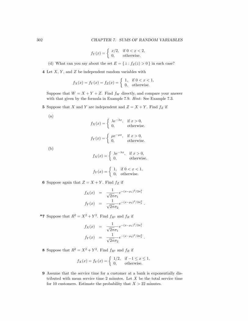
302 CHAPTER 7. SUMS OF RANDOM VARIABLES
fY (x) =x/2, if 0 < x < 2,0, otherwise.
(d) What can you say about the set E = z : fZ(z) > 0 in each case?
4 Let X, Y , and Z be independent random variables with
fX(x) = fY (x) = fZ(x) =
1, if 0 < x < 1,0, otherwise.
Suppose that W = X + Y + Z. Find fW directly, and compare your answerwith that given by the formula in Example 7.9. Hint : See Example 7.3.
5 Suppose that X and Y are independent and Z = X + Y . Find fZ if
(a)
fX(x) =λe−λx, if x > 0,0, otherwise.
fY (x) =µe−µx, if x > 0,0, otherwise.
(b)
fX(x) =λe−λx, if x > 0,0, otherwise.
fY (x) =
1, if 0 < x < 1,0, otherwise.
6 Suppose again that Z = X + Y . Find fZ if
fX(x) =1√
2πσ1
e−(x−µ1)2/2σ21
fY (x) =1√
2πσ2
e−(x−µ2)2/2σ22 .
*7 Suppose that R2 = X2 + Y 2. Find fR2 and fR if
fX(x) =1√
2πσ1
e−(x−µ1)2/2σ21
fY (x) =1√
2πσ2
e−(x−µ2)2/2σ22 .
8 Suppose that R2 = X2 + Y 2. Find fR2 and fR if
fX(x) = fY (x) =
1/2, if −1 ≤ x ≤ 1,0, otherwise.
9 Assume that the service time for a customer at a bank is exponentially dis-tributed with mean service time 2 minutes. Let X be the total service timefor 10 customers. Estimate the probability that X > 22 minutes.

7.2. SUMS OF CONTINUOUS RANDOM VARIABLES 303
10 Let X1, X2, . . . , Xn be n independent random variables each of which hasan exponential density with mean µ. Let M be the minimum value of theXj . Show that the density for M is exponential with mean µ/n. Hint : Usecumulative distribution functions.
11 A company buys 100 lightbulbs, each of which has an exponential lifetime of1000 hours. What is the expected time for the first of these bulbs to burnout? (See Exercise 10.)
12 An insurance company assumes that the time between claims from each of itshomeowners’ policies is exponentially distributed with mean µ. It would liketo estimate µ by averaging the times for a number of policies, but this is notvery practical since the time between claims is about 30 years. At Galambos’5
suggestion the company puts its customers in groups of 50 and observes thetime of the first claim within each group. Show that this provides a practicalway to estimate the value of µ.
13 Particles are subject to collisions that cause them to split into two parts witheach part a fraction of the parent. Suppose that this fraction is uniformlydistributed between 0 and 1. Following a single particle through several split-tings we obtain a fraction of the original particle Zn = X1 ·X2 · . . . ·Xn whereeach Xj is uniformly distributed between 0 and 1. Show that the density forthe random variable Zn is
fn(z) =1
(n− 1)!(− log z)n−1.
Hint : Show that Yk = − logXk is exponentially distributed. Use this to findthe density function for Sn = Y1 +Y2 + · · ·+Yn, and from this the cumulativedistribution and density of Zn = e−Sn .
14 Assume that X1 and X2 are independent random variables, each having anexponential density with parameter λ. Show that Z = X1 −X2 has density
fZ(z) = (1/2)λe−λ|z| .
15 Suppose we want to test a coin for fairness. We flip the coin n times andrecord the number of times X0 that the coin turns up tails and the numberof times X1 = n−X0 that the coin turns up heads. Now we set
Z =1∑i=0
(Xi − n/2)2
n/2.
Then for a fair coin Z has approximately a chi-squared distribution with2 − 1 = 1 degree of freedom. Verify this by computer simulation first for afair coin (p = 1/2) and then for a biased coin (p = 1/3).
5J. Galambos, Introductory Probability Theory (New York: Marcel Dekker, 1984), p. 159.

304 CHAPTER 7. SUMS OF RANDOM VARIABLES
16 Verify your answers in Exercise 2(a) by computer simulation: Choose X andY from [−1, 1] with uniform density and calculate Z = X + Y . Repeat thisexperiment 500 times, recording the outcomes in a bar graph on [−2, 2] with40 bars. Does the density fZ calculated in Exercise 2(a) describe the shapeof your bar graph? Try this for Exercises 2(b) and Exercise 2(c), too.
17 Verify your answers to Exercise 3 by computer simulation.
18 Verify your answer to Exercise 4 by computer simulation.
19 The support of a function f(x) is defined to be the set
x : f(x) > 0 .
Suppose that X and Y are two continuous random variables with densityfunctions fX(x) and fY (y), respectively, and suppose that the supports ofthese density functions are the intervals [a, b] and [c, d], respectively. Find thesupport of the density function of the random variable X + Y .
20 Let X1, X2, . . . , Xn be a sequence of independent random variables, all havinga common density function fX with support [a, b] (see Exercise 19). LetSn = X1 +X2 + · · ·+Xn, with density function fSn . Show that the supportof fSn is the interval [na, nb]. Hint : Write fSn = fSn−1 ∗ fX . Now useExercise 19 to establish the desired result by induction.
21 Let X1, X2, . . . , Xn be a sequence of independent random variables, all havinga common density function fX . Let A = Sn/n be their average. Find fA if
(a) fX(x) = (1/√
2π)e−x2/2 (normal density).
(b) fX(x) = e−x (exponential density).Hint : Write fA(x) in terms of fSn(x).

Chapter 8
Law of Large Numbers
8.1 Law of Large Numbers for Discrete RandomVariables
We are now in a position to prove our first fundamental theorem of probability.We have seen that an intuitive way to view the probability of a certain outcomeis as the frequency with which that outcome occurs in the long run, when the ex-periment is repeated a large number of times. We have also defined probabilitymathematically as a value of a distribution function for the random variable rep-resenting the experiment. The Law of Large Numbers, which is a theorem provedabout the mathematical model of probability, shows that this model is consistentwith the frequency interpretation of probability. This theorem is sometimes calledthe law of averages. To find out what would happen if this law were not true, seethe article by Robert M. Coates.1
Chebyshev Inequality
To discuss the Law of Large Numbers, we first need an important inequality calledthe Chebyshev Inequality.
Theorem 8.1 (Chebyshev Inequality) Let X be a discrete random variablewith expected value µ = E(X), and let ε > 0 be any positive real number. Then
P (|X − µ| ≥ ε) ≤ V (X)ε2
.
Proof. Let m(x) denote the distribution function of X. Then the probability thatX differs from µ by at least ε is given by
P (|X − µ| ≥ ε) =∑|x−µ|≥ε
m(x) .
1R. M. Coates, “The Law,” The World of Mathematics, ed. James R. Newman (New York:Simon and Schuster, 1956.
305

306 CHAPTER 8. LAW OF LARGE NUMBERS
We know that
V (X) =∑x
(x− µ)2m(x) ,
and this is clearly at least as large as∑|x−µ|≥ε
(x− µ)2m(x) ,
since all the summands are positive and we have restricted the range of summationin the second sum. But this last sum is at least∑
|x−µ|≥εε2m(x) = ε2
∑|x−µ|≥ε
m(x)
= ε2P (|X − µ| ≥ ε) .
So,
P (|X − µ| ≥ ε) ≤ V (X)ε2
.
2
Note that X in the above theorem can be any discrete random variable, and ε anypositive number.
Example 8.1 Let X by any random variable with E(X) = µ and V (X) = σ2.Then, if ε = kσ, Chebyshev’s Inequality states that
P (|X − µ| ≥ kσ) ≤ σ2
k2σ2=
1k2
.
Thus, for any random variable, the probability of a deviation from the mean ofmore than k standard deviations is ≤ 1/k2. If, for example, k = 5, 1/k2 = .04. 2
Chebyshev’s Inequality is the best possible inequality in the sense that, for anyε > 0, it is possible to give an example of a random variable for which Chebyshev’sInequality is in fact an equality. To see this, given ε > 0, choose X with distribution
pX =(−ε +ε1/2 1/2
).
Then E(X) = 0, V (X) = ε2, and
P (|X − µ| ≥ ε) =V (X)ε2
= 1 .
We are now prepared to state and prove the Law of Large Numbers.

8.1. DISCRETE RANDOM VARIABLES 307
Law of Large Numbers
Theorem 8.2 (Law of Large Numbers) Let X1, X2, . . . , Xn be an independenttrials process, with finite expected value µ = E(Xj) and finite variance σ2 = V (Xj).Let Sn = X1 +X2 + · · ·+Xn. Then for any ε > 0,
P
(∣∣∣∣Snn − µ∣∣∣∣ ≥ ε)→ 0
as n→∞. Equivalently,
P
(∣∣∣∣Snn − µ∣∣∣∣ < ε
)→ 1
as n→∞.
Proof. Since X1, X2, . . . , Xn are independent and have the same distributions, wecan apply Theorem 6.9. We obtain
V (Sn) = nσ2 ,
and
V (Snn
) =σ2
n.
Also we know thatE(
Snn
) = µ .
By Chebyshev’s Inequality, for any ε > 0,
P
(∣∣∣∣Snn − µ∣∣∣∣ ≥ ε) ≤ σ2
nε2.
Thus, for fixed ε,
P
(∣∣∣∣Snn − µ∣∣∣∣ ≥ ε)→ 0
as n→∞, or equivalently,
P
(∣∣∣∣Snn − µ∣∣∣∣ < ε
)→ 1
as n→∞. 2
Law of Averages
Note that Sn/n is an average of the individual outcomes, and one often calls the Lawof Large Numbers the “law of averages.” It is a striking fact that we can start witha random experiment about which little can be predicted and, by taking averages,obtain an experiment in which the outcome can be predicted with a high degreeof certainty. The Law of Large Numbers, as we have stated it, is often called the“Weak Law of Large Numbers” to distinguish it from the “Strong Law of LargeNumbers” described in Exercise 15.

308 CHAPTER 8. LAW OF LARGE NUMBERS
Consider the important special case of Bernoulli trials with probability p forsuccess. Let Xj = 1 if the jth outcome is a success and 0 if it is a failure. ThenSn = X1 +X2 + · · ·+Xn is the number of successes in n trials and µ = E(X1) = p.The Law of Large Numbers states that for any ε > 0
P
(∣∣∣∣Snn − p∣∣∣∣ < ε
)→ 1
as n → ∞. The above statement says that, in a large number of repetitions of aBernoulli experiment, we can expect the proportion of times the event will occur tobe near p. This shows that our mathematical model of probability agrees with ourfrequency interpretation of probability.
Coin Tossing
Let us consider the special case of tossing a coin n times with Sn the number ofheads that turn up. Then the random variable Sn/n represents the fraction of timesheads turns up and will have values between 0 and 1. The Law of Large Numberspredicts that the outcomes for this random variable will, for large n, be near 1/2.
In Figure 8.1, we have plotted the distribution for this example for increasingvalues of n. We have marked the outcomes between .45 and .55 by dots at the topof the spikes. We see that as n increases the distribution gets more and more con-centrated around .5 and a larger and larger percentage of the total area is containedwithin the interval (.45, .55), as predicted by the Law of Large Numbers.
Die Rolling
Example 8.2 Consider n rolls of a die. Let Xj be the outcome of the jth roll.Then Sn = X1 +X2 + · · ·+Xn is the sum of the first n rolls. This is an independenttrials process with E(Xj) = 7/2. Thus, by the Law of Large Numbers, for any ε > 0
P
(∣∣∣∣Snn − 72
∣∣∣∣ ≥ ε)→ 0
as n→∞. An equivalent way to state this is that, for any ε > 0,
P
(∣∣∣∣Snn − 72
∣∣∣∣ < ε
)→ 1
as n→∞. 2
Numerical Comparisons
It should be emphasized that, although Chebyshev’s Inequality proves the Law ofLarge Numbers, it is actually a very crude inequality for the probabilities involved.However, its strength lies in the fact that it is true for any random variable at all,and it allows us to prove a very powerful theorem.
In the following example, we compare the estimates given by Chebyshev’s In-equality with the actual values.

8.1. DISCRETE RANDOM VARIABLES 309
0 0.2 0.4 0.6 0.8 1
0
0.02
0.04
0.06
0.08
0.1
0 0.2 0.4 0.6 0.8 1
0
0.02
0.04
0.06
0.08
0 0.2 0.4 0.6 0.8 1
0
0.02
0.04
0.06
0.08
0.1
0.12
0.14
0 0.2 0.4 0.6 0.8 1
0
0.02
0.04
0.06
0.08
0.1
0.12
0 0.2 0.4 0.6 0.8 1
0
0.05
0.1
0.15
0.2
0.25
0 0.2 0.4 0.6 0.8 1
0
0.025
0.05
0.075
0.1
0.125
0.15
0.175n=10 n=20
n=40n=30
n=60 n=100
Figure 8.1: Bernoulli trials distributions.

310 CHAPTER 8. LAW OF LARGE NUMBERS
Example 8.3 Let X1, X2, . . . , Xn be a Bernoulli trials process with probability .3for success and .7 for failure. Let Xj = 1 if the jth outcome is a success and 0otherwise. Then, E(Xj) = .3 and V (Xj) = (.3)(.7) = .21. If
An =Snn
=X1 +X2 + · · ·+Xn
n
is the average of the Xi, then E(An) = .3 and V (An) = V (Sn)/n2 = .21/n.Chebyshev’s Inequality states that if, for example, ε = .1,
P (|An − .3| ≥ .1) ≤ .21n(.1)2
=21n.
Thus, if n = 100,P (|A100 − .3| ≥ .1) ≤ .21 ,
or if n = 1000,P (|A1000 − .3| ≥ .1) ≤ .021 .
These can be rewritten as
P (.2 < A100 < .4) ≥ .79 ,
P (.2 < A1000 < .4) ≥ .979 .
These values should be compared with the actual values, which are (to six decimalplaces)
P (.2 < A100 < .4) ≈ .962549
P (.2 < A1000 < .4) ≈ 1 .
The program Law can be used to carry out the above calculations in a systematicway. 2
Historical Remarks
The Law of Large Numbers was first proved by the Swiss mathematician JamesBernoulli in the fourth part of his work Ars Conjectandi published posthumouslyin 1713.2 As often happens with a first proof, Bernoulli’s proof was much moredifficult than the proof we have presented using Chebyshev’s inequality. Cheby-shev developed his inequality to prove a general form of the Law of Large Numbers(see Exercise 12). The inequality itself appeared much earlier in a work by Bien-ayme, and in discussing its history Maistrov remarks that it was referred to as theBienayme-Chebyshev Inequality for a long time.3
In Ars Conjectandi Bernoulli provides his reader with a long discussion of themeaning of his theorem with lots of examples. In modern notation he has an event
2J. Bernoulli, The Art of Conjecturing IV, trans. Bing Sung, Technical Report No. 2, Dept. ofStatistics, Harvard Univ., 1966
3L. E. Maistrov, Probability Theory: A Historical Approach, trans. and ed. Samual Kotz, (NewYork: Academic Press, 1974), p. 202

8.1. DISCRETE RANDOM VARIABLES 311
that occurs with probability p but he does not know p. He wants to estimate pby the fraction p of the times the event occurs when the experiment is repeated anumber of times. He discusses in detail the problem of estimating, by this method,the proportion of white balls in an urn that contains an unknown number of whiteand black balls. He would do this by drawing a sequence of balls from the urn,replacing the ball drawn after each draw, and estimating the unknown proportionof white balls in the urn by the proportion of the balls drawn that are white. Heshows that, by choosing n large enough he can obtain any desired accuracy andreliability for the estimate. He also provides a lively discussion of the applicabilityof his theorem to estimating the probability of dying of a particular disease, ofdifferent kinds of weather occurring, and so forth.
In speaking of the number of trials necessary for making a judgement, Bernoulliobserves that the “man on the street” believes the “law of averages.”
Further, it cannot escape anyone that for judging in this way about anyevent at all, it is not enough to use one or two trials, but rather a greatnumber of trials is required. And sometimes the stupidest man—bysome instinct of nature per se and by no previous instruction (this istruly amazing)— knows for sure that the more observations of this sortthat are taken, the less the danger will be of straying from the mark.4
But he goes on to say that he must contemplate another possibility.
Something futher must be contemplated here which perhaps no one hasthought about till now. It certainly remains to be inquired whetherafter the number of observations has been increased, the probability isincreased of attaining the true ratio between the number of cases inwhich some event can happen and in which it cannot happen, so thatthis probability finally exceeds any given degree of certainty; or whetherthe problem has, so to speak, its own asymptote—that is, whether somedegree of certainty is given which one can never exceed.5
Bernoulli recognized the importance of this theorem, writing:
Therefore, this is the problem which I now set forth and make knownafter I have already pondered over it for twenty years. Both its noveltyand its very great usefullness, coupled with its just as great difficulty,can exceed in weight and value all the remaining chapters of this thesis.6
Bernoulli concludes his long proof with the remark:
Whence, finally, this one thing seems to follow: that if observations ofall events were to be continued throughout all eternity, (and hence theultimate probability would tend toward perfect certainty), everything in
4Bernoulli, op. cit., p. 38.5ibid., p. 39.6ibid., p. 42.

312 CHAPTER 8. LAW OF LARGE NUMBERS
the world would be perceived to happen in fixed ratios and according toa constant law of alternation, so that even in the most accidental andfortuitous occurrences we would be bound to recognize, as it were, acertain necessity and, so to speak, a certain fate.
I do now know whether Plato wished to aim at this in his doctrine ofthe universal return of things, according to which he predicted that allthings will return to their original state after countless ages have past.7
Exercises
1 A fair coin is tossed 100 times. The expected number of heads is 50, and thestandard deviation for the number of heads is (100 · 1/2 · 1/2)1/2 = 5. Whatdoes Chebyshev’s Inequality tell you about the probability that the numberof heads that turn up deviates from the expected number 50 by three or morestandard deviations (i.e., by at least 15)?
2 Write a program that uses the function binomial(n, p, x) to compute the exactprobability that you estimated in Exercise 1. Compare the two results.
3 Write a program to toss a coin 10,000 times. Let Sn be the number of headsin the first n tosses. Have your program print out, after every 1000 tosses,Sn − n/2. On the basis of this simulation, is it correct to say that you canexpect heads about half of the time when you toss a coin a large number oftimes?
4 A 1-dollar bet on craps has an expected winning of −.0141. What does theLaw of Large Numbers say about your winnings if you make a large numberof 1-dollar bets at the craps table? Does it assure you that your losses will besmall? Does it assure you that if n is very large you will lose?
5 Let X be a random variable with E(X) = 0 and V (X) = 1. What integervalue k will assure us that P (|X| ≥ k) ≤ .01?
6 Let Sn be the number of successes in n Bernoulli trials with probability p forsuccess on each trial. Show, using Chebyshev’s Inequality, that for any ε > 0
P
(∣∣∣∣Snn − p∣∣∣∣ ≥ ε) ≤ p(1− p)
nε2.
7 Find the maximum possible value for p(1− p) if 0 < p < 1. Using this resultand Exercise 6, show that the estimate
P
(∣∣∣∣Snn − p∣∣∣∣ ≥ ε) ≤ 1
4nε2
is valid for any p.
7ibid., pp. 65–66.
8.1. DISCRETE RANDOM VARIABLES 313
8 A fair coin is tossed a large number of times. Does the Law of Large Numbersassure us that, if n is large enough, with probability > .99 the number ofheads that turn up will not deviate from n/2 by more than 100?
9 In Exercise 6.2.15, you showed that, for the hat check problem, the numberSn of people who get their own hats back has E(Sn) = V (Sn) = 1. UsingChebyshev’s Inequality, show that P (Sn ≥ 11) ≤ .01 for any n ≥ 11.
10 Let X by any random variable which takes on values 0, 1, 2, . . . , n and hasE(X) = V (X) = 1. Show that, for any integer k,
P (X ≥ k + 1) ≤ 1k2
.
11 We have two coins: one is a fair coin and the other is a coin that producesheads with probability 3/4. One of the two coins is picked at random, and thiscoin is tossed n times. Let Sn be the number of heads that turns up in thesen tosses. Does the Law of Large Numbers allow us to predict the proportionof heads that will turn up in the long run? After we have observed a largenumber of tosses, can we tell which coin was chosen? How many tosses sufficeto make us 95 percent sure?
12 (Chebyshev8) Assume that X1, X2, . . . , Xn are independent random variableswith possibly different distributions and let Sn be their sum. Letmk = E(Xk),σ2k = V (Xk), and Mn = m1 +m2 + · · ·+mn. Assume that σ2
k < R for all k.Prove that, for any ε > 0,
P
(∣∣∣∣Snn − Mn
n
∣∣∣∣ < ε
)→ 1
as n→∞.
13 A fair coin is tossed repeatedly. Before each toss, you are allowed to decidewhether to bet on the outcome. Can you describe a betting system withinfinitely many bets which will enable you, in the long run, to win morethan half of your bets? (Note that we are disallowing a betting system thatsays to bet until you are ahead, then quit.) Write a computer program thatimplements this betting system. As stated above, your program must decidewhether to bet on a particular outcome before that outcome is determined.For example, you might select only outcomes that come after there have beenthree tails in a row. See if you can get more than 50% heads by your “system.”
*14 Prove the following analogue of Chebyshev’s Inequality:
P (|X − E(X)| ≥ ε) ≤ 1εE(|X − E(X)|) .
8P. L. Chebyshev, “On Mean Values,” J. Math. Pure. Appl., vol. 12 (1867), pp. 177–184.

314 CHAPTER 8. LAW OF LARGE NUMBERS
*15 We have proved a theorem often called the “Weak Law of Large Numbers.”Most people’s intuition and our computer simulations suggest that, if we tossa coin a sequence of times, the proportion of heads will really approach 1/2;that is, if Sn is the number of heads in n times, then we will have
An =Snn→ 1
2
as n→∞. Of course, we cannot be sure of this since we are not able to tossthe coin an infinite number of times, and, if we could, the coin could come upheads every time. However, the “Strong Law of Large Numbers,” proved inmore advanced courses, states that
P
(Snn→ 1
2
)= 1 .
Describe a sample space Ω that would make it possible for us to talk aboutthe event
E =ω :
Snn→ 1
2
.
Could we assign the equiprobable measure to this space? (See Example 2.18.)
*16 In this exercise, we shall construct an example of a sequence of random vari-ables that satisfies the weak law of large numbers, but not the strong law.The distribution of Xi will have to depend on i, because otherwise both lawswould be satisfied. (This problem was communicated to us by David Maslen.)
Suppose we have an infinite sequence of mutually independent eventsA1, A2, . . ..Let ai = P (Ai), and let r be a positive integer.
(a) Find an expression of the probability that none of the Ai with i > r
occur.
(b) Use the fact that x− 1 ≤ e−x to show that
P (No Ai with i > r occurs) ≤ e−∑∞
i=rai
(c) (The first Borel-Cantelli lemma) Prove that if∑∞i=1 ai diverges, then
P (infinitely many Ai occur) = 1.
Now, let Xi be a sequence of mutually independent random variablessuch that for each positive integer i ≥ 2,
P (Xi = i) =1
2i log i, P (Xi = −i) =
12i log i
, P (Xi = 0) = 1− 1i log i
.
When i = 1 we let Xi = 0 with probability 1. As usual we let Sn =X1 + · · ·+Xn. Note that the mean of each Xi is 0.

8.1. DISCRETE RANDOM VARIABLES 315
(d) Find the variance of Sn.
(e) Show that the sequence Xi satisfies the Weak Law of Large Numbers,i.e. prove that for any ε > 0
P
(∣∣∣∣Snn∣∣∣∣ ≥ ε)→ 0 ,
as n tends to infinity.
We now show that Xi does not satisfy the Strong Law of Large Num-bers. Suppose that Sn/n→ 0. Then because
Xn
n=Snn− n− 1
n
Sn−1
n− 1,
we know that Xn/n→ 0. From the definition of limits, we conclude thatthe inequality |Xi| ≥ 1
2 i can only be true for finitely many i.
(f) Let Ai be the event |Xi| ≥ 12 i. Find P (Ai). Show that
∑∞i=1 P (Ai)
diverges (use the Integral Test).
(g) Prove that Ai occurs for infinitely many i.
(h) Prove that
P
(Snn→ 0
)= 0,
and hence that the Strong Law of Large Numbers fails for the sequenceXi.
*17 Let us toss a biased coin that comes up heads with probability p and assumethe validity of the Strong Law of Large Numbers as described in Exercise 15.Then, with probability 1,
Snn→ p
as n→∞. If f(x) is a continuous function on the unit interval, then we alsohave
f
(Snn
)→ f(p) .
Finally, we could hope that
E
(f
(Snn
))→ E(f(p)) = f(p) .
Show that, if all this is correct, as in fact it is, we would have proven thatany continuous function on the unit interval is a limit of polynomial func-tions. This is a sketch of a probabilistic proof of an important theorem inmathematics called the Weierstrass approximation theorem.

316 CHAPTER 8. LAW OF LARGE NUMBERS
8.2 Law of Large Numbers for Continuous Ran-dom Variables
In the previous section we discussed in some detail the Law of Large Numbers fordiscrete probability distributions. This law has a natural analogue for continuousprobability distributions, which we consider somewhat more briefly here.
Chebyshev Inequality
Just as in the discrete case, we begin our discussion with the Chebyshev Inequality.
Theorem 8.3 (Chebyshev Inequality) Let X be a continuous random variablewith density function f(x). Suppose X has a finite expected value µ = E(X) andfinite variance σ2 = V (X). Then for any positive number ε > 0 we have
P (|X − µ| ≥ ε) ≤ σ2
ε2.
2
The proof is completely analogous to the proof in the discrete case, and we omitit.
Note that this theorem says nothing if σ2 = V (X) is infinite.
Example 8.4 Let X be any continuous random variable with E(X) = µ andV (X) = σ2. Then, if ε = kσ = k standard deviations for some integer k, then
P (|X − µ| ≥ kσ) ≤ σ2
k2σ2=
1k2
,
just as in the discrete case. 2
Law of Large Numbers
With the Chebyshev Inequality we can now state and prove the Law of LargeNumbers for the continuous case.
Theorem 8.4 (Law of Large Numbers) Let X1, X2, . . . , Xn be an independenttrials process with a continuous density function f , finite expected value µ, and finitevariance σ2. Let Sn = X1 +X2 + · · ·+Xn be the sum of the Xi. Then for any realnumber ε > 0 we have
limn→∞
P
(∣∣∣∣Snn − µ∣∣∣∣ ≥ ε) = 0 ,
or equivalently,
limn→∞
P
(∣∣∣∣Snn − µ∣∣∣∣ < ε
)= 1 .
2

8.2. CONTINUOUS RANDOM VARIABLES 317
Note that this theorem is not necessarily true if σ2 is infinite (see Example 8.8).As in the discrete case, the Law of Large Numbers says that the average value
of n independent trials tends to the expected value as n→∞, in the precise sensethat, given ε > 0, the probability that the average value and the expected valuediffer by more than ε tends to 0 as n→∞.
Once again, we suppress the proof, as it is identical to the proof in the discretecase.
Uniform Case
Example 8.5 Suppose we choose at random n numbers from the interval [0, 1]with uniform distribution. Then if Xi describes the ith choice, we have
µ = E(Xi) =∫ 1
0
x dx =12,
σ2 = V (Xi) =∫ 1
0
x2 dx− µ2
=13− 1
4=
112
.
Hence,
E
(Snn
)=
12,
V
(Snn
)=
112n
,
and for any ε > 0,
P
(∣∣∣∣Snn − 12
∣∣∣∣ ≥ ε) ≤ 112nε2
.
This says that if we choose n numbers at random from [0, 1], then the chancesare better than 1− 1/(12nε2) that the difference |Sn/n− 1/2| is less than ε. Notethat ε plays the role of the amount of error we are willing to tolerate: If we chooseε = 0.1, say, then the chances that |Sn/n − 1/2| is less than 0.1 are better than1 − 100/(12n). For n = 100, this is about .92, but if n = 1000, this is better than.99 and if n = 10,000, this is better than .999.
We can illustrate what the Law of Large Numbers says for this example graph-ically. The density for An = Sn/n is determined by
fAn(x) = nfSn(nx) .
We have seen in Section 7.2, that we can compute the density fSn(x) for thesum of n uniform random variables. In Figure 8.2 we have used this to plot thedensity for An for various values of n. We have shaded in the area for which Anwould lie between .45 and .55. We see that as we increase n, we obtain more andmore of the total area inside the shaded region. The Law of Large Numbers tells usthat we can obtain as much of the total area as we please inside the shaded regionby choosing n large enough (see also Figure 8.1). 2

318 CHAPTER 8. LAW OF LARGE NUMBERS
n=2 n=5 n=10
n=20 n=30 n=50
Figure 8.2: Illustration of Law of Large Numbers — uniform case.
Normal Case
Example 8.6 Suppose we choose n real numbers at random, using a normal dis-tribution with mean 0 and variance 1. Then
µ = E(Xi) = 0 ,
σ2 = V (Xi) = 1 .
Hence,
E
(Snn
)= 0 ,
V
(Snn
)=
1n,
and, for any ε > 0,
P
(∣∣∣∣Snn − 0∣∣∣∣ ≥ ε) ≤ 1
nε2.
In this case it is possible to compare the Chebyshev estimate for P (|Sn/n−µ| ≥ ε)in the Law of Large Numbers with exact values, since we know the density functionfor Sn/n exactly (see Example 7.9). The comparison is shown in Table 8.1, forε = .1. The data in this table was produced by the program LawContinuous. Wesee here that the Chebyshev estimates are in general not very accurate. 2

8.2. CONTINUOUS RANDOM VARIABLES 319
n P (|Sn/n| ≥ .1) Chebyshev100 .31731 1.00000200 .15730 .50000300 .08326 .33333400 .04550 .25000500 .02535 .20000600 .01431 .16667700 .00815 .14286800 .00468 .12500900 .00270 .11111
1000 .00157 .10000
Table 8.1: Chebyshev estimates.
Monte Carlo Method
Here is a somewhat more interesting example.
Example 8.7 Let g(x) be a continuous function defined for x ∈ [0, 1] with valuesin [0, 1]. In Section 2.1, we showed how to estimate the area of the region underthe graph of g(x) by the Monte Carlo method, that is, by choosing a large numberof random values for x and y with uniform distribution and seeing what fraction ofthe points P (x, y) fell inside the region under the graph (see Example 2.2).
Here is a better way to estimate the same area (see Figure 8.3). Let us choose alarge number of independent values Xn at random from [0, 1] with uniform density,set Yn = g(Xn), and find the average value of the Yn. Then this average is ourestimate for the area. To see this, note that if the density function for Xn isuniform,
µ = E(Yn) =∫ 1
0
g(x)f(x) dx
=∫ 1
0
g(x) dx
= average value of g(x) ,
while the variance is
σ2 = E((Yn − µ)2) =∫ 1
0
(g(x)− µ)2 dx < 1 ,
since for all x in [0, 1], g(x) is in [0, 1], hence µ is in [0, 1], and so |g(x) − µ| ≤ 1.Now let An = (1/n)(Y1 + Y2 + · · ·+ Yn). Then by Chebyshev’s Inequality, we have
P (|An − µ| ≥ ε) ≤σ2
nε2<
1nε2
.
This says that to get within ε of the true value for µ =∫ 1
0g(x) dx with probability
at least p, we should choose n so that 1/nε2 ≤ 1− p (i.e., so that n ≥ 1/ε2(1− p)).Note that this method tells us how large to take n to get a desired accuracy. 2

320 CHAPTER 8. LAW OF LARGE NUMBERS
Y
X
Y = g (x)
0
1
1
Figure 8.3: Area problem.
The Law of Large Numbers requires that the variance σ2 of the original under-lying density be finite: σ2 <∞. In cases where this fails to hold, the Law of LargeNumbers may fail, too. An example follows.
Cauchy Case
Example 8.8 Suppose we choose n numbers from (−∞,+∞) with a Cauchy den-sity with parameter a = 1. We know that for the Cauchy density the expected valueand variance are undefined (see Example 6.28). In this case, the density functionfor
An =Snn
is given by (see Example 7.6)
fAn(x) =1
π(1 + x2),
that is, the density function for An is the same for all n. In this case, as n increases,the density function does not change at all, and the Law of Large Numbers doesnot hold. 2
Exercises
1 Let X be a continuous random variable with mean µ = 10 and varianceσ2 = 100/3. Using Chebyshev’s Inequality, find an upper bound for thefollowing probabilities.

8.2. CONTINUOUS RANDOM VARIABLES 321
(a) P (|X − 10| ≥ 2).
(b) P (|X − 10| ≥ 5).
(c) P (|X − 10| ≥ 9).
(d) P (|X − 10| ≥ 20).
2 Let X be a continuous random variable with values unformly distributed overthe interval [0, 20].
(a) Find the mean and variance of X.
(b) Calculate P (|X − 10| ≥ 2), P (|X − 10| ≥ 5), P (|X − 10| ≥ 9), andP (|X − 10| ≥ 20) exactly. How do your answers compare with those ofExercise 1? How good is Chebyshev’s Inequality in this case?
3 Let X be the random variable of Exercise 2.
(a) Calculate the function f(x) = P (|X − 10| ≥ x).
(b) Now graph the function f(x), and on the same axes, graph the Chebyshevfunction g(x) = 100/(3x2). Show that f(x) ≤ g(x) for all x > 0, butthat g(x) is not a very good approximation for f(x).
4 Let X be a continuous random variable with values exponentially distributedover [0,∞) with parameter λ = 0.1.
(a) Find the mean and variance of X.
(b) Using Chebyshev’s Inequality, find an upper bound for the followingprobabilities: P (|X − 10| ≥ 2), P (|X − 10| ≥ 5), P (|X − 10| ≥ 9), andP (|X − 10| ≥ 20).
(c) Calculate these probabilities exactly, and compare with the bounds in(b).
5 Let X be a continuous random variable with values normally distributed over(−∞,+∞) with mean µ = 0 and variance σ2 = 1.
(a) Using Chebyshev’s Inequality, find upper bounds for the following prob-abilities: P (|X| ≥ 1), P (|X| ≥ 2), and P (|X| ≥ 3).
(b) The area under the normal curve between −1 and 1 is .6827, between−2 and 2 is .9545, and between −3 and 3 it is .9973 (see the table inAppendix A). Compare your bounds in (a) with these exact values. Howgood is Chebyshev’s Inequality in this case?
6 If X is normally distributed, with mean µ and variance σ2, find an upperbound for the following probabilities, using Chebyshev’s Inequality.
(a) P (|X − µ| ≥ σ).
(b) P (|X − µ| ≥ 2σ).
(c) P (|X − µ| ≥ 3σ).

322 CHAPTER 8. LAW OF LARGE NUMBERS
(d) P (|X − µ| ≥ 4σ).
Now find the exact value using the program NormalArea or the normal tablein Appendix A, and compare.
7 If X is a random variable with mean µ 6= 0 and variance σ2, define the relativedeviation D of X from its mean by
D =∣∣∣∣X − µµ
∣∣∣∣ .(a) Show that P (D ≥ a) ≤ σ2/(µ2a2).
(b) If X is the random variable of Exercise 1, find an upper bound for P (D ≥.2), P (D ≥ .5), P (D ≥ .9), and P (D ≥ 2).
8 Let X be a continuous random variable and define the standardized versionX∗ of X by:
X∗ =X − µσ
.
(a) Show that P (|X∗| ≥ a) ≤ 1/a2.
(b) If X is the random variable of Exercise 1, find bounds for P (|X∗| ≥ 2),P (|X∗| ≥ 5), and P (|X∗| ≥ 9).
9 (a) Suppose a number X is chosen at random from [0, 20] with uniformprobability. Find a lower bound for the probability that X lies between8 and 12, using Chebyshev’s Inequality.
(b) Now suppose 20 real numbers are chosen independently from [0, 20] withuniform probability. Find a lower bound for the probability that theiraverage lies between 8 and 12.
(c) Now suppose 100 real numbers are chosen independently from [0, 20].Find a lower bound for the probability that their average lies between8 and 12.
10 A student’s score on a particular calculus final is a random variable with valuesof [0, 100], mean 70, and variance 25.
(a) Find a lower bound for the probability that the student’s score will fallbetween 65 and 75.
(b) If 100 students take the final, find a lower bound for the probability thatthe class average will fall between 65 and 75.
11 The Pilsdorff beer company runs a fleet of trucks along the 100 mile road fromHangtown to Dry Gulch, and maintains a garage halfway in between. Eachof the trucks is apt to break down at a point X miles from Hangtown, whereX is a random variable uniformly distributed over [0, 100].
(a) Find a lower bound for the probability P (|X − 50| ≤ 10).

8.2. CONTINUOUS RANDOM VARIABLES 323
(b) Suppose that in one bad week, 20 trucks break down. Find a lower boundfor the probability P (|A20 − 50| ≤ 10), where A20 is the average of thedistances from Hangtown at the time of breakdown.
12 A share of common stock in the Pilsdorff beer company has a price Yn onthe nth business day of the year. Finn observes that the price change Xn =Yn+1 − Yn appears to be a random variable with mean µ = 0 and varianceσ2 = 1/4. If Y1 = 30, find a lower bound for the following probabilities, underthe assumption that the Xn’s are mutually independent.
(a) P (25 ≤ Y2 ≤ 35).
(b) P (25 ≤ Y11 ≤ 35).
(c) P (25 ≤ Y101 ≤ 35).
13 Suppose one hundred numbers X1, X2, . . . , X100 are chosen independently atrandom from [0, 20]. Let S = X1 + X2 + · · · + X100 be the sum, A = S/100the average, and S∗ = (S − 1000)/(10/
√3) the standardized sum. Find lower
bounds for the probabilities
(a) P (|S − 1000| ≤ 100).
(b) P (|A− 10| ≤ 1).
(c) P (|S∗| ≤√
3).
14 Let X be a continuous random variable normally distributed on (−∞,+∞)with mean 0 and variance 1. Using the normal table provided in Appendix A,or the program NormalArea, find values for the function f(x) = P (|X| ≥ x)as x increases from 0 to 4.0 in steps of .25. Note that for x ≥ 0 the table givesNA(0, x) = P (0 ≤ X ≤ x) and thus P (|X| ≥ x) = 2(.5 −NA(0, x). Plot byhand the graph of f(x) using these values, and the graph of the Chebyshevfunction g(x) = 1/x2, and compare (see Exercise 3).
15 Repeat Exercise 14, but this time with mean 10 and variance 3. Note thatthe table in Appendix A presents values for a standard normal variable. Findthe standardized version X∗ for X, find values for f∗(x) = P (|X∗| ≥ x) as inExercise 14, and then rescale these values for f(x) = P (|X − 10| ≥ x). Graphand compare this function with the Chebyshev function g(x) = 3/x2.
16 Let Z = X/Y where X and Y have normal densities with mean 0 and standarddeviation 1. Then it can be shown that Z has a Cauchy density.
(a) Write a program to illustrate this result by plotting a bar graph of 1000samples obtained by forming the ratio of two standard normal outcomes.Compare your bar graph with the graph of the Cauchy density. Depend-ing upon which computer language you use, you may or may not need totell the computer how to simulate a normal random variable. A methodfor doing this was described in Section 5.2.

324 CHAPTER 8. LAW OF LARGE NUMBERS
(b) We have seen that the Law of Large Numbers does not apply to theCauchy density (see Example 8.8). Simulate a large number of experi-ments with Cauchy density and compute the average of your results. Dothese averages seem to be approaching a limit? If so can you explainwhy this might be?
17 Show that, if X ≥ 0, then P (X ≥ a) ≤ E(X)/a.
18 (Lamperti9) Let X be a non-negative random variable. What is the bestupper bound you can give for P (X ≥ a) if you know
(a) E(X) = 20.
(b) E(X) = 20 and V (X) = 25.
(c) E(X) = 20, V (X) = 25, and X is symmetric about its mean.
9Private communication.

Chapter 9
Central Limit Theorem
9.1 Central Limit Theorem for Bernoulli Trials
The second fundamental theorem of probability is the Central Limit Theorem. Thistheorem says that if Sn is the sum of n mutually independent random variables, thenthe distribution function of Sn is well-approximated by a certain type of continuousfunction known as a normal density function, which is given by the formula
fµ,σ(x) =1√2πσ
e−(x−µ)2/(2σ2) ,
as we have seen in Chapter 4.3. In this section, we will deal only with the case thatµ = 0 and σ = 1. We will call this particular normal density function the standardnormal density, and we will denote it by φ(x):
φ(x) =1√2πe−x
2/2 .
A graph of this function is given in Figure 9.1. It can be shown that the area underany normal density equals 1.
The Central Limit Theorem tells us, quite generally, what happens when wehave the sum of a large number of independent random variables each of which con-tributes a small amount to the total. In this section we shall discuss this theoremas it applies to the Bernoulli trials and in Section 9.2 we shall consider more generalprocesses. We will discuss the theorem in the case that the individual random vari-ables are identically distributed, but the theorem is true, under certain conditions,even if the individual random variables have different distributions.
Bernoulli Trials
Consider a Bernoulli trials process with probability p for success on each trial.Let Xi = 1 or 0 according as the ith outcome is a success or failure, and letSn = X1 +X2 + · · ·+Xn. Then Sn is the number of successes in n trials. We knowthat Sn has as its distribution the binomial probabilities b(n, p, j). In Section 3.2,
325

326 CHAPTER 9. CENTRAL LIMIT THEOREM
-4 -2 0 2 4
0
0.1
0.2
0.3
0.4
Figure 9.1: Standard normal density.
we plotted these distributions for p = .3 and p = .5 for various values of n (seeFigure 3.5).
We note that the maximum values of the distributions appeared near the ex-pected value np, which causes their spike graphs to drift off to the right as n in-creased. Moreover, these maximum values approach 0 as n increased, which causesthe spike graphs to flatten out.
Standardized Sums
We can prevent the drifting of these spike graphs by subtracting the expected num-ber of successes np from Sn, obtaining the new random variable Sn − np. Now themaximum values of the distributions will always be near 0.
To prevent the spreading of these spike graphs, we can normalize Sn−np to havevariance 1 by dividing by its standard deviation
√npq (see Exercise 6.2.12 and Ex-
ercise 6.2.16).
Definition 9.1 The standardized sum of Sn is given by
S∗n =Sn − np√
npq.
S∗n always has expected value 0 and variance 1. 2
Suppose we plot a spike graph with the spikes placed at the possible values of S∗n:x0, x1, . . . , xn, where
xj =j − np√npq
. (9.1)
We make the height of the spike at xj equal to the distribution value b(n, p, j). Anexample of this standardized spike graph, with n = 270 and p = .3, is shown inFigure 9.2. This graph is beautifully bell-shaped. We would like to fit a normaldensity to this spike graph. The obvious choice to try is the standard normal density,since it is centered at 0, just as the standardized spike graph is. In this figure, we

9.1. BERNOULLI TRIALS 327
-4 -2 0 2 40
0.1
0.2
0.3
0.4
Figure 9.2: Normalized binomial distribution and standard normal density.
have drawn this standard normal density. The reader will note that a horrible thinghas occurred: Even though the shapes of the two graphs are the same, the heightsare quite different.
If we want the two graphs to fit each other, we must modify one of them; wechoose to modify the spike graph. Since the shapes of the two graphs look fairlyclose, we will attempt to modify the spike graph without changing its shape. Thereason for the differing heights is that the sum of the heights of the spikes equals1, while the area under the standard normal density equals 1. If we were to draw acontinuous curve through the top of the spikes, and find the area under this curve,we see that we would obtain, approximately, the sum of the heights of the spikesmultiplied by the distance between consecutive spikes, which we will call ε. Sincethe sum of the heights of the spikes equals one, the area under this curve would beapproximately ε. Thus, to change the spike graph so that the area under this curvehas value 1, we need only multiply the heights of the spikes by 1/ε. It is easy to seefrom Equation 9.1 that
ε =1√npq
.
In Figure 9.3 we show the standardized sum S∗n for n = 270 and p = .3, aftercorrecting the heights, together with the standard normal density. (This figure wasproduced with the program CLTBernoulliPlot.) The reader will note that thestandard normal fits the height-corrected spike graph extremely well. In fact, oneversion of the Central Limit Theorem (see Theorem 9.1) says that as n increases,the standard normal density will do an increasingly better job of approximatingthe height-corrected spike graphs corresponding to a Bernoulli trials process withn summands.
Let us fix a value x on the x-axis and let n be a fixed positive integer. Then,using Equation 9.1, the point xj that is closest to x has a subscript j given by the

328 CHAPTER 9. CENTRAL LIMIT THEOREM
-4 -2 0 2 40
0.1
0.2
0.3
0.4
Figure 9.3: Corrected spike graph with standard normal density.
formulaj = 〈np+ x
√npq〉 ,
where 〈a〉 means the integer nearest to a. Thus the height of the spike above xjwill be √
npq b(n, p, j) =√npq b(n, p, 〈np+ xj
√npq〉) .
For large n, we have seen that the height of the spike is very close to the height ofthe normal density at x. This suggests the following theorem.
Theorem 9.1 (Central Limit Theorem for Binomial Distributions) For thebinomial distribution b(n, p, j) we have
limn→∞
√npq b(n, p, 〈np+ x
√npq〉) = φ(x) ,
where φ(x) is the standard normal density.The proof of this theorem can be carried out using Stirling’s approximation from
Section 3.1. We indicate this method of proof by considering the case x = 0. Inthis case, the theorem states that
limn→∞
√npq b(n, p, 〈np〉) =
1√2π
= .3989 . . . .
In order to simplify the calculation, we assume that np is an integer, so that 〈np〉 =np. Then
√npq b(n, p, np) =
√npq pnpqnq
n!(np)! (nq)!
.
Recall that Stirling’s formula (see Theorem 3.3) states that
n! ∼√
2πnnne−n as n→∞ .

9.1. BERNOULLI TRIALS 329
Using this, we have
√npq b(n, p, np) ∼
√npq pnpqnq
√2πnnne−n√
2πnp√
2πnq (np)np(nq)nqe−npe−nq,
which simplifies to 1/√
2π. 2
Approximating Binomial Distributions
We can use Theorem 9.1 to find approximations for the values of binomial distri-bution functions. If we wish to find an approximation for b(n, p, j), we set
j = np+ x√npq
and solve for x, obtaining
x =j − np√npq
.
Theorem 9.1 then says that √npq b(n, p, j)
is approximately equal to φ(x), so
b(n, p, j) ≈ φ(x)√npq
=1√npq
φ
(j − np√npq
).
Example 9.1 Let us estimate the probability of exactly 55 heads in 100 tosses ofa coin. For this case np = 100 · 1/2 = 50 and
√npq =
√100 · 1/2 · 1/2 = 5. Thus
x55 = (55− 50)/5 = 1 and
P (S100 = 55) ∼ φ(1)5
=15
(1√2πe−1/2
)= .0484 .
To four decimal places, the actual value is .0485, and so the approximation isvery good. 2
The program CLTBernoulliLocal illustrates this approximation for any choiceof n, p, and j. We have run this program for two examples. The first is theprobability of exactly 50 heads in 100 tosses of a coin; the estimate is .0798, while theactual value, to four decimal places, is .0796. The second example is the probabilityof exactly eight sixes in 36 rolls of a die; here the estimate is .1093, while the actualvalue, to four decimal places, is .1196.

330 CHAPTER 9. CENTRAL LIMIT THEOREM
The individual binomial probabilities tend to 0 as n tends to infinity. In mostapplications we are not interested in the probability that a specific outcome occurs,but rather in the probability that the outcome lies in a given interval, say the interval[a, b]. In order to find this probability, we add the heights of the spike graphs forvalues of j between a and b. This is the same as asking for the probability that thestandardized sum S∗n lies between a∗ and b∗, where a∗ and b∗ are the standardizedvalues of a and b. But as n tends to infinity the sum of these areas could be expectedto approach the area under the standard normal density between a∗ and b∗. TheCentral Limit Theorem states that this does indeed happen.
Theorem 9.2 (Central Limit Theorem for Bernoulli Trials) Let Sn be thenumber of successes in n Bernoulli trials with probability p for success, and let aand b be two fixed real numbers. Define
a∗ =a− np√npq
andb∗ =
b− np√npq
.
Then
limn→∞
P (a ≤ Sn ≤ b) =∫ b∗
a∗φ(x) dx .
2
This theorem can be proved by adding together the approximations to b(n, p, k)given in Theorem 9.1.It is also a special case of the more general Central LimitTheorem (see Section 10.3).
We know from calculus that the integral on the right side of this equation isequal to the area under the graph of the standard normal density φ(x) betweena and b. We denote this area by NA(a∗, b∗). Unfortunately, there is no simple wayto integrate the function e−x
2/2, and so we must either use a table of values or elsea numerical integration program. (See Figure 9.4 for values of NA(0, z). A moreextensive table is given in Appendix A.)
It is clear from the symmetry of the standard normal density that areas such asthat between −2 and 3 can be found from this table by adding the area from 0 to 2(same as that from −2 to 0) to the area from 0 to 3.
Approximation of Binomial Probabilities
Suppose that Sn is binomially distributed with parameters n and p. We have seenthat the above theorem shows how to estimate a probability of the form
P (i ≤ Sn ≤ j) , (9.2)
where i and j are integers between 0 and n. As we have seen, the binomial distri-bution can be represented as a spike graph, with spikes at the integers between 0and n, and with the height of the kth spike given by b(n, p, k). For moderate-sized

9.1. BERNOULLI TRIALS 331
NA (0,z) = area of shaded region
0 z
z NA(z) z NA(z) z NA(z) z NA(z)
.0 .0000 1.0 .3413 2.0 .4772 3.0 .4987
.1 .0398 1.1 .3643 2.1 .4821 3.1 .4990
.2 .0793 1.2 .3849 2.2 .4861 3.2 .4993
.3 .1179 1.3 .4032 2.3 .4893 3.3 .4995
.4 .1554 1.4 .4192 2.4 .4918 3.4 .4997
.5 .1915 1.5 .4332 2.5 .4938 3.5 .4998
.6 .2257 1.6 .4452 2.6 .4953 3.6 .4998
.7 .2580 1.7 .4554 2.7 .4965 3.7 .4999
.8 .2881 1.8 .4641 2.8 .4974 3.8 .4999
.9 .3159 1.9 .4713 2.9 .4981 3.9 .5000
Figure 9.4: Table of values of NA(0, z), the normal area from 0 to z.

332 CHAPTER 9. CENTRAL LIMIT THEOREM
values of n, if we standardize this spike graph, and change the heights of its spikes,in the manner described above, the sum of the heights of the spikes is approximatedby the area under the standard normal density between i∗ and j∗. It turns out thata slightly more accurate approximation is afforded by the area under the standardnormal density between the standardized values corresponding to (i − 1/2) and(j + 1/2); these values are
i∗ =i− 1/2− np√
npq
and
j∗ =j + 1/2− np√
npq.
Thus,
P (i ≤ Sn ≤ j) ≈ NA
(i− 1
2 − np√npq
,j + 1
2 − np√npq
).
We now illustrate this idea with some examples.
Example 9.2 A coin is tossed 100 times. Estimate the probability that the numberof heads lies between 40 and 60 (the word “between” in mathematics means inclusiveof the endpoints). The expected number of heads is 100 ·1/2 = 50, and the standarddeviation for the number of heads is
√100 · 1/2 · 1/2 = 5. Thus, since n = 100 is
reasonably large, we have
P (40 ≤ Sn ≤ 60) ≈ P
(39.5− 50
5≤ S∗n ≤
60.5− 505
)= P (−2.1 ≤ S∗n ≤ 2.1)
≈ NA(−2.1, 2.1)
= 2NA(0, 2.1)
≈ .9642 .
The actual value is .96480, to five decimal places.Note that in this case we are asking for the probability that the outcome will
not deviate by more than two standard deviations from the expected value. Hadwe asked for the probability that the number of successes is between 35 and 65, thiswould have represented three standard deviations from the mean, and, using our1/2 correction, our estimate would be the area under the standard normal curvebetween −3.1 and 3.1, or 2NA(0, 3.1) = .9980. The actual answer in this case, tofive places, is .99821. 2
It is important to work a few problems by hand to understand the conversionfrom a given inequality to an inequality relating to the standardized variable. Afterthis, one can then use a computer program that carries out this conversion, includingthe 1/2 correction. The program CLTBernoulliGlobal is such a program forestimating probabilities of the form P (a ≤ Sn ≤ b).

9.1. BERNOULLI TRIALS 333
Example 9.3 Dartmouth College would like to have 1050 freshmen. This collegecannot accommodate more than 1060. Assume that each applicant accepts withprobability .6 and that the acceptances can be modeled by Bernoulli trials. If thecollege accepts 1700, what is the probability that it will have too many acceptances?
If it accepts 1700 students, the expected number of students who matricu-late is .6 · 1700 = 1020. The standard deviation for the number that accept is√
1700 · .6 · .4 ≈ 20. Thus we want to estimate the probability
P (S1700 > 1060) = P (S1700 ≥ 1061)
= P
(S∗1700 ≥
1060.5− 102020
)= P (S∗1700 ≥ 2.025) .
From Table 9.4, if we interpolate, we would estimate this probability to be.5− .4784 = .0216. Thus, the college is fairly safe using this admission policy. 2
Applications to Statistics
There are many important questions in the field of statistics that can be answeredusing the Central Limit Theorem for independent trials processes. The followingexample is one that is encountered quite frequently in the news. Another exampleof an application of the Central Limit Theorem to statistics is given in Section 9.2.
Example 9.4 One frequently reads that a poll has been taken to estimate theproportion of people in a certain population who favor one candidate over anotherin a race with two candidates. (This model also applies to races with more thantwo candidates A and B, and to ballot propositions.) Clearly, it is not possible forpollsters to ask everyone for their preference. What is done instead is to pick asubset of the population, called a sample, and ask everyone in the sample for theirpreference. Let p be the actual proportion of people in the population who are infavor of candidate A and let q = 1−p. If we choose a sample of size n from the pop-ulation, the preferences of the people in the sample can be represented by randomvariables X1, X2, . . . , Xn, where Xi = 1 if person i is in favor of candidate A, andXi = 0 if person i is in favor of candidate B. Let Sn = X1 +X2 + · · ·+Xn. If eachsubset of size n is chosen with the same probability, then Sn is hypergeometricallydistributed. If n is small relative to the size of the population (which is typicallytrue in practice), then Sn is approximately binomially distributed, with parametersn and p.
The pollster wants to estimate the value p. An estimate for p is provided by thevalue p = Sn/n, which is the proportion of people in the sample who favor candidateB. The Central Limit Theorem says that the random variable p is approximatelynormally distributed. (In fact, our version of the Central Limit Theorem says thatthe distribution function of the random variable
S∗n =Sn − np√
npq

334 CHAPTER 9. CENTRAL LIMIT THEOREM
is approximated by the standard normal density.) But we have
p =Sn − np√
npq
√pq
n+ p ,
i.e., p is just a linear function of S∗n. Since the distribution of S∗n is approximatedby the standard normal density, the distribution of the random variable p must alsobe bell-shaped. We also know how to write the mean and standard deviation of pin terms of p and n. The mean of p is just p, and the standard deviation is√
pq
n.
Thus, it is easy to write down the standardized version of p; it is
p∗ =p− p√pq/n
.
Since the distribution of the standardized version of p is approximated by thestandard normal density, we know, for example, that 95% of its values will lie withintwo standard deviations of its mean, and the same is true of p. So we have
P
(p− 2
√pq
n< p < p+ 2
√pq
n
)≈ .954 .
Now the pollster does not know p or q, but he can use p and q = 1 − p in theirplace without too much danger. With this idea in mind, the above statement isequivalent to the statement
P
(p− 2
√pq
n< p < p+ 2
√pq
n
)≈ .954 .
The resulting interval (p− 2
√pq√n, p+
2√pq√n
)is called the 95 percent confidence interval for the unknown value of p. The nameis suggested by the fact that if we use this method to estimate p in a large numberof samples we should expect that in about 95 percent of the samples the true valueof p is contained in the confidence interval obtained from the sample. In Exercise 11you are asked to write a program to illustrate that this does indeed happen.
The pollster has control over the value of n. Thus, if he wants to create a 95%confidence interval with length 6%, then he should choose a value of n so that
2√pq√n≤ .03 .
Using the fact that pq ≤ 1/4, no matter what the value of p is, it is easy to showthat if he chooses a value of n so that
1√n≤ .03 ,

9.1. BERNOULLI TRIALS 335
0.48 0.5 0.52 0.54 0.56 0.58 0.6
0
5
10
15
20
25
Figure 9.5: Polling simulation.
he will be safe. This is equivalent to choosing
n ≥ 1111 .
So if the pollster chooses n to be 1200, say, and calculates p using his sample of size1200, then 19 times out of 20 (i.e., 95% of the time), his confidence interval, whichis of length 6%, will contain the true value of p. This type of confidence intervalis typically reported in the news as follows: this survey has a 3% margin of error.In fact, most of the surveys that one sees reported in the paper will have samplesizes around 1000. A somewhat surprising fact is that the size of the population hasapparently no effect on the sample size needed to obtain a 95% confidence intervalfor p with a given margin of error. To see this, note that the value of n that wasneeded depended only on the number .03, which is the margin of error. In otherwords, whether the population is of size 100,000 or 100,000,000, the pollster needsonly to choose a sample of size 1200 or so to get the same accuracy of estimate ofp. (We did use the fact that the sample size was small relative to the populationsize in the statement that Sn is approximately binomially distributed.)
In Figure 9.5, we show the results of simulating the polling process. The popula-tion is of size 100,000, and for the population, p = .54. The sample size was chosento be 1200. The spike graph shows the distribution of p for 10,000 randomly chosensamples. For this simulation, the program kept track of the number of samples forwhich p was within 3% of .54. This number was 9648, which is close to 95% of thenumber of samples used.
Another way to see what the idea of confidence intervals means is shown inFigure 9.6. In this figure, we show 100 confidence intervals, obtained by computingp for 100 different samples of size 1200 from the same population as before. Thereader can see that most of these confidence intervals (96, to be exact) contain thetrue value of p.

336 CHAPTER 9. CENTRAL LIMIT THEOREM
0.48 0.5 0.52 0.54 0.56 0.58 0.6
Figure 9.6: Confidence interval simulation.
The Gallup Poll has used these polling techniques in every Presidential electionsince 1936 (and in innumerable other elections as well). Table 9.11 shows the resultsof their efforts. The reader will note that most of the approximations to p are within3% of the actual value of p. The sample sizes for these polls were typically around1500. (In the table, both the predicted and actual percentages for the winningcandidate refer to the percentage of the vote among the “major” political parties.In most elections, there were two major parties, but in several elections, there werethree.)
This technique also plays an important role in the evaluation of the effectivenessof drugs in the medical profession. For example, it is sometimes desired to knowwhat proportion of patients will be helped by a new drug. This proportion canbe estimated by giving the drug to a subset of the patients, and determining theproportion of this sample who are helped by the drug. 2
Historical Remarks
The Central Limit Theorem for Bernoulli trials was first proved by Abrahamde Moivre and appeared in his book, The Doctrine of Chances, first publishedin 1718.2
De Moivre spent his years from age 18 to 21 in prison in France because of hisProtestant background. When he was released he left France for England, wherehe worked as a tutor to the sons of noblemen. Newton had presented a copy ofhis Principia Mathematica to the Earl of Devonshire. The story goes that, while
1The Gallup Poll Monthly, November 1992, No. 326, p. 33. Supplemented with the help ofLydia K. Saab, The Gallup Organization.
2A. de Moivre, The Doctrine of Chances, 3d ed. (London: Millar, 1756).

9.1. BERNOULLI TRIALS 337
Year Winning Gallup Final Election DeviationCandidate Survey Result
1936 Roosevelt 55.7% 62.5% 6.8%1940 Roosevelt 52.0% 55.0% 3.0%1944 Roosevelt 51.5% 53.3% 1.8%1948 Truman 44.5% 49.9% 5.4%1952 Eisenhower 51.0% 55.4% 4.4%1956 Eisenhower 59.5% 57.8% 1.7%1960 Kennedy 51.0% 50.1% 0.9%1964 Johnson 64.0% 61.3% 2.7%1968 Nixon 43.0% 43.5% 0.5%1972 Nixon 62.0% 61.8% 0.2%1976 Carter 48.0% 50.0% 2.0%1980 Reagan 47.0% 50.8% 3.8%1984 Reagan 59.0% 59.1% 0.1%1988 Bush 56.0% 53.9% 2.1%1992 Clinton 49.0% 43.2% 5.8%1996 Clinton 52.0% 50.1% 1.9%
Table 9.1: Gallup Poll accuracy record.
de Moivre was tutoring at the Earl’s house, he came upon Newton’s work and foundthat it was beyond him. It is said that he then bought a copy of his own and toreit into separate pages, learning it page by page as he walked around London to histutoring jobs. De Moivre frequented the coffeehouses in London, where he startedhis probability work by calculating odds for gamblers. He also met Newton at such acoffeehouse and they became fast friends. De Moivre dedicated his book to Newton.
The Doctrine of Chances provides the techniques for solving a wide variety ofgambling problems. In the midst of these gambling problems de Moivre rathermodestly introduces his proof of the Central Limit Theorem, writing
A Method of approximating the Sum of the Terms of the Binomial(a + b)n expanded into a Series, from whence are deduced some prac-tical Rules to estimate the Degree of Assent which is to be given toExperiments.3
De Moivre’s proof used the approximation to factorials that we now call Stirling’sformula. De Moivre states that he had obtained this formula before Stirling butwithout determining the exact value of the constant
√2π. While he says it is not
really necessary to know this exact value, he concedes that knowing it “has spreada singular Elegancy on the Solution.”
The complete proof and an interesting discussion of the life of de Moivre can befound in the book Games, Gods and Gambling by F. N. David.4
3ibid., p. 243.4F. N. David, Games, Gods and Gambling (London: Griffin, 1962).

338 CHAPTER 9. CENTRAL LIMIT THEOREM
Exercises
1 Let S100 be the number of heads that turn up in 100 tosses of a fair coin. Usethe Central Limit Theorem to estimate
(a) P (S100 ≤ 45).
(b) P (45 < S100 < 55).
(c) P (S100 > 63).
(d) P (S100 < 57).
2 Let S200 be the number of heads that turn up in 200 tosses of a fair coin.Estimate
(a) P (S200 = 100).
(b) P (S200 = 90).
(c) P (S200 = 80).
3 A true-false examination has 48 questions. June has probability 3/4 of an-swering a question correctly. April just guesses on each question. A passingscore is 30 or more correct answers. Compare the probability that June passesthe exam with the probability that April passes it.
4 Let S be the number of heads in 1,000,000 tosses of a fair coin. Use (a) Cheby-shev’s inequality, and (b) the Central Limit Theorem, to estimate the prob-ability that S lies between 499,500 and 500,500. Use the same two methodsto estimate the probability that S lies between 499,000 and 501,000, and theprobability that S lies between 498,500 and 501,500.
5 A rookie is brought to a baseball club on the assumption that he will have a.300 batting average. (Batting average is the ratio of the number of hits to thenumber of times at bat.) In the first year, he comes to bat 300 times and hisbatting average is .267. Assume that his at bats can be considered Bernoullitrials with probability .3 for success. Could such a low average be consideredjust bad luck or should he be sent back to the minor leagues? Comment onthe assumption of Bernoulli trials in this situation.
6 Once upon a time, there were two railway trains competing for the passengertraffic of 1000 people leaving from Chicago at the same hour and going to LosAngeles. Assume that passengers are equally likely to choose each train. Howmany seats must a train have to assure a probability of .99 or better of havinga seat for each passenger?
7 Assume that, as in Example 9.3, Dartmouth admits 1750 students. What isthe probability of too many acceptances?
8 A club serves dinner to members only. They are seated at 12-seat tables. Themanager observes over a long period of time that 95 percent of the time thereare between six and nine full tables of members, and the remainder of the

9.1. BERNOULLI TRIALS 339
time the numbers are equally likely to fall above or below this range. Assumethat each member decides to come with a given probability p, and that thedecisions are independent. How many members are there? What is p?
9 Let Sn be the number of successes in n Bernoulli trials with probability .8 forsuccess on each trial. Let An = Sn/n be the average number of successes. Ineach case give the value for the limit, and give a reason for your answer.
(a) limn→∞ P (An = .8).
(b) limn→∞ P (.7n < Sn < .9n).
(c) limn→∞ P (Sn < .8n+ .8√n).
(d) limn→∞ P (.79 < An < .81).
10 Find the probability that among 10,000 random digits the digit 3 appears notmore than 931 times.
11 Write a computer program to simulate 10,000 Bernoulli trials with probabil-ity .3 for success on each trial. Have the program compute the 95 percentconfidence interval for the probability of success based on the proportion ofsuccesses. Repeat the experiment 100 times and see how many times the truevalue of .3 is included within the confidence limits.
12 A balanced coin is flipped 400 times. Determine the number x such thatthe probability that the number of heads is between 200 − x and 200 + x isapproximately .80.
13 A noodle machine in Spumoni’s spaghetti factory makes about 5 percent de-fective noodles even when properly adjusted. The noodles are then packedin crates containing 1900 noodles each. A crate is examined and found tocontain 115 defective noodles. What is the approximate probability of findingat least this many defective noodles if the machine is properly adjusted?
14 A restaurant feeds 400 customers per day. On the average 20 percent of thecustomers order apple pie.
(a) Give a range (called a 95 percent confidence interval) for the number ofpieces of apple pie ordered on a given day such that you can be 95 percentsure that the actual number will fall in this range.
(b) How many customers must the restaurant have, on the average, to be atleast 95 percent sure that the number of customers ordering pie on thatday falls in the 19 to 21 percent range?
15 Recall that if X is a random variable, the cumulative distribution functionof X is the function F (x) defined by
F (x) = P (X ≤ x) .
(a) Let Sn be the number of successes in n Bernoulli trials with probability pfor success. Write a program to plot the cumulative distribution for Sn.

340 CHAPTER 9. CENTRAL LIMIT THEOREM
(b) Modify your program in (a) to plot the cumulative distribution F ∗n(x) ofthe standardized random variable
S∗n =Sn − np√
npq.
(c) Define the normal distribution N(x) to be the area under the normalcurve up to the value x. Modify your program in (b) to plot the normaldistribution as well, and compare it with the cumulative distributionof S∗n. Do this for n = 10, 50, and 100.
16 In Example 3.11, we were interested in testing the hypothesis that a new formof aspirin is effective 80 percent of the time rather than the 60 percent of thetime as reported for standard aspirin. The new aspirin is given to n people.If it is effective in m or more cases, we accept the claim that the new drugis effective 80 percent of the time and if not we reject the claim. Using theCentral Limit Theorem, show that you can choose the number of trials n andthe critical value m so that the probability that we reject the hypothesis whenit is true is less than .01 and the probability that we accept it when it is falseis also less than .01. Find the smallest value of n that will suffice for this.
17 In an opinion poll it is assumed that an unknown proportion p of the peopleare in favor of a proposed new law and a proportion 1 − p are against it.A sample of n people is taken to obtain their opinion. The proportion p infavor in the sample is taken as an estimate of p. Using the Central LimitTheorem, determine how large a sample will ensure that the estimate will,with probability .95, be correct to within .01.
18 A description of a poll in a certain newspaper says that one can be 95%confident that error due to sampling will be no more than plus or minus 3percentage points. A poll in the New York Times taken in Iowa says that“according to statistical theory, in 19 out of 20 cases the results based on suchsamples will differ by no more than 3 percentage points in either directionfrom what would have been obtained by interviewing all adult Iowans.” Theseare both attempts to explain the concept of confidence intervals. Do bothstatements say the same thing? If not, which do you think is the more accuratedescription?
9.2 Central Limit Theorem for Discrete Indepen-dent Trials
We have illustrated the Central Limit Theorem in the case of Bernoulli trials, butthis theorem applies to a much more general class of chance processes. In particular,it applies to any independent trials process such that the individual trials have finitevariance. For such a process, both the normal approximation for individual termsand the Central Limit Theorem are valid.

9.2. DISCRETE INDEPENDENT TRIALS 341
Let Sn = X1 + X2 + · · · + Xn be the sum of n independent discrete randomvariables of an independent trials process with common distribution function m(x)defined on the integers, with mean µ and variance σ2. We have seen in Section 7.2that the distributions for such independent sums have shapes resembling the nor-mal curve, but the largest values drift to the right and the curves flatten out (seeFigure 7.6). We can prevent this just as we did for Bernoulli trials.
Standardized Sums
Consider the standardized random variable
S∗n =Sn − nµ√
nσ2.
This standardizes Sn to have expected value 0 and variance 1. If Sn = j, thenS∗n has the value xj with
xj =j − nµ√nσ2
.
We can construct a spike graph just as we did for Bernoulli trials. Each spike iscentered at some xj . The distance between successive spikes is
b =1√nσ2
,
and the height of the spike is
h =√nσ2P (Sn = j) .
The case of Bernoulli trials is the special case for which Xj = 1 if the jthoutcome is a success and 0 otherwise; then µ = p and σ2 =
√pq.
We now illustrate this process for two different discrete distributions. The firstis the distribution m, given by
m =(
1 2 3 4 5.2 .2 .2 .2 .2
).
In Figure 9.7 we show the standardized sums for this distribution for the casesn = 2 and n = 10. Even for n = 2 the approximation is surprisingly good.
For our second discrete distribution, we choose
m =(
1 2 3 4 5.4 .3 .1 .1 .1
).
This distribution is quite asymmetric and the approximation is not very goodfor n = 3, but by n = 10 we again have an excellent approximation (see Figure 9.8).Figures 9.7 and 9.8 were produced by the program CLTIndTrialsPlot.

342 CHAPTER 9. CENTRAL LIMIT THEOREM
-4 -2 0 2 40
0.1
0.2
0.3
0.4
-4 -2 0 2 40
0.1
0.2
0.3
0.4n = 2 n = 10
Figure 9.7: Distribution of standardized sums.
-4 -2 0 2 40
0.1
0.2
0.3
0.4
-4 -2 0 2 40
0.1
0.2
0.3
0.4n = 3 n = 10
Figure 9.8: Distribution of standardized sums.
Approximation Theorem
As in the case of Bernoulli trials, these graphs suggest the following approximationtheorem for the individual probabilities.
Theorem 9.3 Let X1, X2, . . . , Xn be an independent trials process and let Sn =X1 +X2 + · · ·+Xn. Assume that the greatest common divisor of the differences ofall the values that the Xj can take on is 1. Let E(Xj) = µ and V (Xj) = σ2. Thenfor n large,
P (Sn = j) ∼ φ(xj)√nσ2
,
where xj = (j − nµ)/√nσ2, and φ(x) is the standard normal density. 2
The program CLTIndTrialsLocal implements this approximation. When werun this program for 6 rolls of a die, and ask for the probability that the sum of therolls equals 21, we obtain an actual value of .09285, and a normal approximationvalue of .09537. If we run this program for 24 rolls of a die, and ask for theprobability that the sum of the rolls is 72, we obtain an actual value of .01724and a normal approximation value of .01705. These results show that the normalapproximations are quite good.

9.2. DISCRETE INDEPENDENT TRIALS 343
Central Limit Theorem for a Discrete Independent Trials Pro-cess
The Central Limit Theorem for a discrete independent trials process is as follows.
Theorem 9.4 (Central Limit Theorem) Let Sn = X1 +X2 + · · ·+Xn be thesum of n discrete independent random variables with common distribution havingexpected value µ and variance σ2. Then, for a < b,
limn→∞
P
(a <
Sn − nµ√nσ2
< b
)=
1√2π
∫ b
a
e−x2/2 dx .
2
We will give the proofs of Theorems 9.3 and Theorem 9.4 in Section 10.3. Herewe consider several examples.
Examples
Example 9.5 A die is rolled 420 times. What is the probability that the sum ofthe rolls lies between 1400 and 1550?
The sum is a random variable
S420 = X1 +X2 + · · ·+X420 ,
where each Xj has distribution
mX =(
1 2 3 4 5 61/6 1/6 1/6 1/6 1/6 1/6
)We have seen that µ = E(X) = 7/2 and σ2 = V (X) = 35/12. Thus, E(S420) =420 · 7/2 = 1470, σ2(S420) = 420 · 35/12 = 1225, and σ(S420) = 35. Therefore,
P (1400 ≤ S420 ≤ 1550) ≈ P
(1399.5− 1470
35≤ S∗240 ≤
1550.5− 147035
)= P (−2.01 ≤ S∗420 ≤ 2.30)
≈ NA(−2.01, 2.30) = .9670 .
We note that the program CLTIndTrialsGlobal could be used to calculate theseprobabilities. 2
Example 9.6 A student’s grade point average is the average of his grades in 30courses. The grades are based on 100 possible points and are recorded as integers.Assume that, in each course, the instructor makes an error in grading of k withprobability |p/k|, where k = ±1, ±2, ±3, ±4, ±5. The probability of no error isthen 1− (137/30)p. (The parameter p represents the inaccuracy of the instructor’sgrading.) Thus, in each course, there are two grades for the student, namely the

344 CHAPTER 9. CENTRAL LIMIT THEOREM
“correct” grade and the recorded grade. So there are two average grades for thestudent, namely the average of the correct grades and the average of the recordedgrades.
We wish to estimate the probability that these two average grades differ by lessthan .05 for a given student. We now assume that p = 1/20. We also assumethat the total error is the sum S30 of 30 independent random variables each withdistribution
mX :−5 −4 −3 −2 −1 0 1 2 3 4 51
100180
160
140
120
463600
120
140
160
180
1100
.
One can easily calculate that E(X) = 0 and σ2(X) = 1.5. Then we have
P(−.05 ≤ S30
30 ≤ .05)
= P (−1.5 ≤ S30 ≤ 1.5)
= P(−1.5√30·1.5 ≤ S
∗30 ≤ 1.5√
30·1.5
)= P (−.224 ≤ S∗30 ≤ .224)
≈ NA(−.224, .224) = .1772 .
This means that there is only a 17.7% chance that a given student’s grade pointaverage is accurate to within .05. (Thus, for example, if two candidates for valedic-torian have recorded averages of 97.1 and 97.2, there is an appreciable probabilitythat their correct averages are in the reverse order.) For a further discussion of thisexample, see the article by R. M. Kozelka.5 2
A More General Central Limit Theorem
In Theorem 9.4, the discrete random variables that were being summed were as-sumed to be independent and identically distributed. It turns out that the assump-tion of identical distributions can be substantially weakened. Much work has beendone in this area, with an important contribution being made by J. W. Lindeberg.Lindeberg found a condition on the sequence Xn which guarantees that the dis-tribution of the sum Sn is asymptotically normally distributed. Feller showed thatLindeberg’s condition is necessary as well, in the sense that if the condition doesnot hold, then the sum Sn is not asymptotically normally distributed. For a pre-cise statement of Lindeberg’s Theorem, we refer the reader to Feller.6 A sufficientcondition that is stronger (but easier to state) than Lindeberg’s condition, and isweaker than the condition in Theorem 9.4, is given in the following theorem.
5R. M. Kozelka, “Grade-Point Averages and the Central Limit Theorem,” American Math.Monthly, vol. 86 (Nov 1979), pp. 773-777.
6W. Feller, Introduction to Probability Theory and its Applications, vol. 1, 3rd ed. (New York:John Wiley & Sons, 1968), p. 254.

9.2. DISCRETE INDEPENDENT TRIALS 345
Theorem 9.5 (Central Limit Theorem) Let X1, X2, . . . , Xn , . . . be a se-quence of independent discrete random variables, and let Sn = X1 +X2 + · · ·+Xn.For each n, denote the mean and variance of Xn by µn and σ2
n, respectively. De-fine the mean and variance of Sn to be mn and s2
n, respectively, and assume thatsn →∞. If there exists a constant A, such that |Xn| ≤ A for all n, then for a < b,
limn→∞
P
(a <
Sn −mn
sn< b
)=
1√2π
∫ b
a
e−x2/2 dx .
2
The condition that |Xn| ≤ A for all n is sometimes described by saying that thesequence Xn is uniformly bounded. The condition that sn →∞ is necessary (seeExercise 15).
We illustrate this theorem by generating a sequence of n random distributions onthe interval [a, b]. We then convolute these distributions to find the distribution ofthe sum of n experiments governed by these distributions. Finally, we standardizedthe distribution for the sum to have mean 0 and standard deviation 1 and compareit with the normal density. The program CLTGeneral carries out this procedure.
In Figure 9.9 we show the result of running this program for [a, b] = [−2, 4], andn = 1, 4, and 10. We see that our first random distribution is quite asymmetric.By the time we choose the sum of ten such experiments we have a very good fit tothe normal curve.
The above theorem essentially says that anything that can be thought of as beingmade up as the sum of many small independent pieces is approximately normallydistributed. This brings us to one of the most important questions that was askedabout genetics in the 1800’s.
The Normal Distribution and Genetics
When one looks at the distribution of heights of adults of one sex in a given pop-ulation, one cannot help but notice that this distribution looks like the normaldistribution. An example of this is shown in Figure 9.10. This figure shows thedistribution of heights of 9593 women between the ages of 21 and 74. These datacome from the Health and Nutrition Examination Survey I (HANES I). For thissurvey, a sample of the U.S. civilian population was chosen. The survey was carriedout between 1971 and 1974.
A natural question to ask is “How does this come about?”. Francis Galton,an English scientist in the 19th century, studied this question, and other relatedquestions, and constructed probability models that were of great importance inexplaining the genetic effects on such attributes as height. In fact, one of the mostimportant ideas in statistics, the idea of regression to the mean, was invented byGalton in his attempts to understand these genetic effects.
Galton was faced with an apparent contradiction. On the one hand, he knewthat the normal distribution arises in situations in which many small independenteffects are being summed. On the other hand, he also knew that many quantitativeattributes, such as height, are strongly influenced by genetic factors: tall parents

346 CHAPTER 9. CENTRAL LIMIT THEOREM
-4 -2 0 2 40
0.1
0.2
0.3
0.4
0.5
0.6
-4 -2 0 2 40
0.1
0.2
0.3
0.4
-4 -2 0 2 40
0.1
0.2
0.3
0.4
Figure 9.9: Sums of randomly chosen random variables.

9.2. DISCRETE INDEPENDENT TRIALS 347
50 55 60 65 70 75 80
0
0.025
0.05
0.075
0.1
0.125
0.15
Figure 9.10: Distribution of heights of adult women.
tend to have tall offspring. Thus in this case, there seem to be two large effects,namely the parents. Galton was certainly aware of the fact that non-genetic factorsplayed a role in determining the height of an individual. Nevertheless, unless thesenon-genetic factors overwhelm the genetic ones, thereby refuting the hypothesisthat heredity is important in determining height, it did not seem possible for sets ofparents of given heights to have offspring whose heights were normally distributed.
One can express the above problem symbolically as follows. Suppose that wechoose two specific positive real numbers x and y, and then find all pairs of parentsone of whom is x units tall and the other of whom is y units tall. We then lookat all of the offspring of these pairs of parents. One can postulate the existence ofa function f(x, y) which denotes the genetic effect of the parents’ heights on theheights of the offspring. One can then let W denote the effects of the non-geneticfactors on the heights of the offspring. Then, for a given set of heights x, y, therandom variable which represents the heights of the offspring is given by
H = f(x, y) +W ,
where f is a deterministic function, i.e., it gives one output for a pair of inputsx, y. If we assume that the effect of f is large in comparison with the effect ofW , then the variance of W is small. But since f is deterministic, the variance of Hequals the variance of W , so the variance of H is small. However, Galton observedfrom his data that the variance of the heights of the offspring of a given pair ofparent heights is not small. This would seem to imply that inheritance plays asmall role in the determination of the height of an individual. Later in this section,we will describe the way in which Galton got around this problem.
We will now consider the modern explanation of why certain traits, such asheights, are approximately normally distributed. In order to do so, we need tointroduce some terminology from the field of genetics. The cells in a living organismthat are not directly involved in the transmission of genetic material to offspringare called somatic cells, and the remaining cells are called germ cells. Organisms ofa given species have their genetic information encoded in sets of physical entities,

348 CHAPTER 9. CENTRAL LIMIT THEOREM
called chromosomes. The chromosomes are paired in each somatic cell. For example,human beings have 23 pairs of chromosomes in each somatic cell. The sex cellscontain one chromosome from each pair. In sexual reproduction, two sex cells, onefrom each parent, contribute their chromosomes to create the set of chromosomesfor the offspring.
Chromosomes contain many subunits, called genes. Genes consist of moleculesof DNA, and one gene has, encoded in its DNA, information that leads to the reg-ulation of proteins. In the present context, we will consider those genes containinginformation that has an effect on some physical trait, such as height, of the organ-ism. The pairing of the chromosomes gives rise to a pairing of the genes on thechromosomes.
In a given species, each gene can be any one of several forms. These variousforms are called alleles. One should think of the different alleles as potentiallyproducing different effects on the physical trait in question. Of the two alleles thatare found in a given gene pair in an organism, one of the alleles came from oneparent and the other allele came from the other parent. The possible types of pairsof alleles (without regard to order) are called genotypes.
If we assume that the height of a human being is largely controlled by a specificgene, then we are faced with the same difficulty that Galton was. We are assumingthat each parent has a pair of alleles which largely controls their heights. Sinceeach parent contributes one allele of this gene pair to each of its offspring, there arefour possible allele pairs for the offspring at this gene location. The assumption isthat these pairs of alleles largely control the height of the offspring, and we are alsoassuming that genetic factors outweigh non-genetic factors. It follows that amongthe offspring we should see several modes in the height distribution of the offspring,one mode corresponding to each possible pair of alleles. This distribution does notcorrespond to the observed distribution of heights.
An alternative hypothesis, which does explain the observation of normally dis-tributed heights in offspring of a given sex, is the multiple-gene hypothesis. Underthis hypothesis, we assume that there are many genes that affect the height of anindividual. These genes may differ in the amount of their effects. Thus, we canrepresent each gene pair by a random variable Xi, where the value of the randomvariable is the allele pair’s effect on the height of the individual. Thus, for example,if each parent has two different alleles in the gene pair under consideration, thenthe offspring has one of four possible pairs of alleles at this gene location. Now theheight of the offspring is a random variable, which can be expressed as
H = X1 +X2 + · · ·+Xn +W ,
if there are n genes that affect height. (Here, as before, the random variable W de-notes non-genetic effects.) Although n is fixed, if it is fairly large, then Theorem 9.5implies that the sum X1 + X2 + · · · + Xn is approximately normally distributed.Now, if we assume that the Xi’s have a significantly larger cumulative effect thanW does, then H is approximately normally distributed.
Another observed feature of the distribution of heights of adults of one sex ina population is that the variance does not seem to increase or decrease from one
9.2. DISCRETE INDEPENDENT TRIALS 349
generation to the next. This was known at the time of Galton, and his attemptsto explain this led him to the idea of regression to the mean. This idea will bediscussed further in the historical remarks at the end of the section. (The reasonthat we only consider one sex is that human heights are clearly sex-linked, and ingeneral, if we have two populations that are each normally distributed, then theirunion need not be normally distributed.)
Using the multiple-gene hypothesis, it is easy to explain why the variance shouldbe constant from generation to generation. We begin by assuming that for a specificgene location, there are k alleles, which we will denote by A1, A2, . . . , Ak. Weassume that the offspring are produced by random mating. By this we mean thatgiven any offspring, it is equally likely that it came from any pair of parents in thepreceding generation. There is another way to look at random mating that makesthe calculations easier. We consider the set S of all of the alleles (at the given genelocation) in all of the germ cells of all of the individuals in the parent generation.In terms of the set S, by random mating we mean that each pair of alleles in S isequally likely to reside in any particular offspring. (The reader might object to thisway of thinking about random mating, as it allows two alleles from the same parentto end up in an offspring; but if the number of individuals in the parent populationis large, then whether or not we allow this event does not affect the probabilitiesvery much.)
For 1 ≤ i ≤ k, we let pi denote the proportion of alleles in the parent populationthat are of type Ai. It is clear that this is the same as the proportion of alleles in thegerm cells of the parent population, assuming that each parent produces roughlythe same number of germs cells. Consider the distribution of alleles in the offspring.Since each germ cell is equally likely to be chosen for any particular offspring, thedistribution of alleles in the offspring is the same as in the parents.
We next consider the distribution of genotypes in the two generations. We willprove the following fact: the distribution of genotypes in the offspring generationdepends only upon the distribution of alleles in the parent generation (in particular,it does not depend upon the distribution of genotypes in the parent generation).Consider the possible genotypes; there are k(k + 1)/2 of them. Under our assump-tions, the genotype AiAi will occur with frequency p2
i , and the genotype AiAj ,with i 6= j, will occur with frequency 2pipj . Thus, the frequencies of the genotypesdepend only upon the allele frequencies in the parent generation, as claimed.
This means that if we start with a certain generation, and a certain distributionof alleles, then in all generations after the one we started with, both the alleledistribution and the genotype distribution will be fixed. This last statement isknown as the Hardy-Weinberg Law.
We can describe the consequences of this law for the distribution of heightsamong adults of one sex in a population. We recall that the height of an offspringwas given by a random variable H, where
H = X1 +X2 + · · ·+Xn +W ,
with the Xi’s corresponding to the genes that affect height, and the random variableW denoting non-genetic effects. The Hardy-Weinberg Law states that for each Xi,

350 CHAPTER 9. CENTRAL LIMIT THEOREM
the distribution in the offspring generation is the same as the distribution in theparent generation. Thus, if we assume that the distribution of W is roughly thesame from generation to generation (or if we assume that its effects are small), thenthe distribution of H is the same from generation to generation. (In fact, dietaryeffects are part of W , and it is clear that in many human populations, diets havechanged quite a bit from one generation to the next in recent times. This change isthought to be one of the reasons that humans, on the average, are getting taller. Itis also the case that the effects of W are thought to be small relative to the geneticeffects of the parents.)
Discussion
Generally speaking, the Central Limit Theorem contains more information thanthe Law of Large Numbers, because it gives us detailed information about theshape of the distribution of S∗n; for large n the shape is approximately the sameas the shape of the standard normal density. More specifically, the Central LimitTheorem says that if we standardize and height-correct the distribution of Sn, thenthe normal density function is a very good approximation to this distribution whenn is large. Thus, we have a computable approximation for the distribution for Sn,which provides us with a powerful technique for generating answers for all sortsof questions about sums of independent random variables, even if the individualrandom variables have different distributions.
Historical Remarks
In the mid-1800’s, the Belgian mathematician Quetelet7 had shown empirically thatthe normal distribution occurred in real data, and had also given a method for fittingthe normal curve to a given data set. Laplace8 had shown much earlier that thesum of many independent identically distributed random variables is approximatelynormal. Galton knew that certain physical traits in a population appeared to beapproximately normally distributed, but he did not consider Laplace’s result to bea good explanation of how this distribution comes about. We give a quote fromGalton that appears in the fascinating book by S. Stigler9 on the history of statistics:
First, let me point out a fact which Quetelet and all writers who havefollowed in his paths have unaccountably overlooked, and which has anintimate bearing on our work to-night. It is that, although characteris-tics of plants and animals conform to the law, the reason of their doingso is as yet totally unexplained. The essence of the law is that differencesshould be wholly due to the collective actions of a host of independentpetty influences in various combinations...Now the processes of hered-ity...are not petty influences, but very important ones...The conclusionis...that the processes of heredity must work harmoniously with the lawof deviation, and be themselves in some sense conformable to it.
7S. Stigler, The History of Statistics, (Cambridge: Harvard University Press, 1986), p. 203.8ibid., p. 1369ibid., p. 281.

9.2. DISCRETE INDEPENDENT TRIALS 351
Figure 9.11: Two-stage version of the quincunx.
Galton invented a device known as a quincunx (now commonly called a Galtonboard), which we used in Example 3.10 to show how to physically obtain a binomialdistribution. Of course, the Central Limit Theorem says that for large values ofthe parameter n, the binomial distribution is approximately normal. Galton usedthe quincunx to explain how inheritance affects the distribution of a trait amongoffspring.
We consider, as Galton did, what happens if we interrupt, at some intermediateheight, the progress of the shot that is falling in the quincunx. The reader is referredto Figure 9.11. This figure is a drawing of Karl Pearson,10 based upon Galton’snotes. In this figure, the shot is being temporarily segregated into compartments atthe line AB. (The line A′B′ forms a platform on which the shot can rest.) If the lineAB is not too close to the top of the quincunx, then the shot will be approximatelynormally distributed at this line. Now suppose that one compartment is opened, asshown in the figure. The shot from that compartment will fall, forming a normaldistribution at the bottom of the quincunx. If now all of the compartments areopened, all of the shot will fall, producing the same distribution as would occur ifthe shot were not temporarily stopped at the line AB. But the action of stoppingthe shot at the line AB, and then releasing the compartments one at a time, isjust the same as convoluting two normal distributions. The normal distributions atthe bottom, corresponding to each compartment at the line AB, are being mixed,with their weights being the number of shot in each compartment. On the otherhand, it is already known that if the shot are unimpeded, the final distribution isapproximately normal. Thus, this device shows that the convolution of two normaldistributions is again normal.
Galton also considered the quincunx from another perspective. He segregatedinto seven groups, by weight, a set of 490 sweet pea seeds. He gave 10 seeds fromeach of the seven group to each of seven friends, who grew the plants from theseeds. Galton found that each group produced seeds whose weights were normally
10Karl Pearson, The Life, Letters and Labours of Francis Galton, vol. IIIB, (Cambridge at theUniversity Press 1930.) p. 466. Reprinted with permission.

352 CHAPTER 9. CENTRAL LIMIT THEOREM
distributed. (The sweet pea reproduces by self-pollination, so he did not need toconsider the possibility of interaction between different groups.) In addition, hefound that the variances of the weights of the offspring were the same for eachgroup. This segregation into groups corresponds to the compartments at the lineAB in the quincunx. Thus, the sweet peas were acting as though they were beinggoverned by a convolution of normal distributions.
He now was faced with a problem. We have shown in Chapter 7, and Galtonknew, that the convolution of two normal distributions produces a normal distribu-tion with a larger variance than either of the original distributions. But his data onthe sweet pea seeds showed that the variance of the offspring population was thesame as the variance of the parent population. His answer to this problem was topostulate a mechanism that he called reversion, and is now called regression to themean. As Stigler puts it:11
The seven groups of progeny were normally distributed, but not abouttheir parents’ weight. Rather they were in every case distributed abouta value that was closer to the average population weight than was that ofthe parent. Furthermore, this reversion followed “the simplest possiblelaw,” that is, it was linear. The average deviation of the progeny fromthe population average was in the same direction as that of the parent,but only a third as great. The mean progeny reverted to type, andthe increased variation was just sufficient to maintain the populationvariability.
Galton illustrated reversion with the illustration shown in Figure 9.12.12 Theparent population is shown at the top of the figure, and the slanted lines are meantto correspond to the reversion effect. The offspring population is shown at thebottom of the figure.
Exercises
1 A die is rolled 24 times. Use the Central Limit Theorem to estimate theprobability that
(a) the sum is greater than 84.
(b) the sum is equal to 84.
2 A random walker starts at 0 on the x-axis and at each time unit moves 1step to the right or 1 step to the left with probability 1/2. Estimate theprobability that, after 100 steps, the walker is more than 10 steps from thestarting position.
3 A piece of rope is made up of 100 strands. Assume that the breaking strengthof the rope is the sum of the breaking strengths of the individual strands.
11ibid., p. 282.12Karl Pearson, The Life, Letters and Labours of Francis Galton, vol. IIIA, (Cambridge at the
University Press 1930.) p. 9. Reprinted with permission.

9.2. DISCRETE INDEPENDENT TRIALS 353
Figure 9.12: Galton’s explanation of reversion.

354 CHAPTER 9. CENTRAL LIMIT THEOREM
Assume further that this sum may be considered to be the sum of an inde-pendent trials process with 100 experiments each having expected value of 10pounds and standard deviation 1. Find the approximate probability that therope will support a weight
(a) of 1000 pounds.
(b) of 970 pounds.
4 Write a program to find the average of 1000 random digits 0, 1, 2, 3, 4, 5, 6, 7,8, or 9. Have the program test to see if the average lies within three standarddeviations of the expected value of 4.5. Modify the program so that it repeatsthis simulation 1000 times and keeps track of the number of times the test ispassed. Does your outcome agree with the Central Limit Theorem?
5 A die is thrown until the first time the total sum of the face values of the dieis 700 or greater. Estimate the probability that, for this to happen,
(a) more than 210 tosses are required.
(b) less than 190 tosses are required.
(c) between 180 and 210 tosses, inclusive, are required.
6 A bank accepts rolls of pennies and gives 50 cents credit to a customer withoutcounting the contents. Assume that a roll contains 49 pennies 30 percent ofthe time, 50 pennies 60 percent of the time, and 51 pennies 10 percent of thetime.
(a) Find the expected value and the variance for the amount that the bankloses on a typical roll.
(b) Estimate the probability that the bank will lose more than 25 cents in100 rolls.
(c) Estimate the probability that the bank will lose exactly 25 cents in 100rolls.
(d) Estimate the probability that the bank will lose any money in 100 rolls.
(e) How many rolls does the bank need to collect to have a 99 percent chanceof a net loss?
7 A surveying instrument makes an error of −2, −1, 0, 1, or 2 feet with equalprobabilities when measuring the height of a 200-foot tower.
(a) Find the expected value and the variance for the height obtained usingthis instrument once.
(b) Estimate the probability that in 18 independent measurements of thistower, the average of the measurements is between 199 and 201, inclusive.
8 For Example 9.6 estimate P (S30 = 0). That is, estimate the probability thatthe errors cancel out and the student’s grade point average is correct.

9.3. CONTINUOUS INDEPENDENT TRIALS 355
9 Prove the Law of Large Numbers using the Central Limit Theorem.
10 Peter and Paul match pennies 10,000 times. Describe briefly what each of thefollowing theorems tells you about Peter’s fortune.
(a) The Law of Large Numbers.
(b) The Central Limit Theorem.
11 A tourist in Las Vegas was attracted by a certain gambling game in whichthe customer stakes 1 dollar on each play; a win then pays the customer2 dollars plus the return of her stake, although a loss costs her only her stake.Las Vegas insiders, and alert students of probability theory, know that theprobability of winning at this game is 1/4. When driven from the tables byhunger, the tourist had played this game 240 times. Assuming that no nearmiracles happened, about how much poorer was the tourist upon leaving thecasino? What is the probability that she lost no money?
12 We have seen that, in playing roulette at Monte Carlo (Example 6.13), betting1 dollar on red or 1 dollar on 17 amounts to choosing between the distributions
mX =(−1 −1/2 1
18/37 1/37 18/37
)or
mX =(−1 35
36/37 1/37
)You plan to choose one of these methods and use it to make 100 1-dollar betsusing the method chosen. Which gives you the higher probability of winningat least 20 dollars? Which gives you the higher probability of winning anymoney?
13 In Example 9.6 find the largest value of p that gives probability .954 that thefirst decimal place is correct.
14 It has been suggested that Example 9.6 is unrealistic, in the sense that theprobabilities of errors are too low. Make up your own (reasonable) estimatefor the distribution m(x), and determine the probability that a student’s gradepoint average is accurate to within .05. Also determine the probability thatit is accurate to within .5.
15 Find a sequence of uniformly bounded discrete independent random variablesXn such that the variance of their sum does not tend to ∞ as n→∞, andsuch that their sum is not asymptotically normally distributed.
9.3 Central Limit Theorem for Continuous Inde-pendent Trials
We have seen in Section 9.2 that the distribution function for the sum of a largenumber n of independent discrete random variables with mean µ and variance σ2

356 CHAPTER 9. CENTRAL LIMIT THEOREM
tends to look like a normal density with mean nµ and variance nσ2. What isremarkable about this result is that it holds for any distribution with finite meanand variance. We shall see in this section that the same result also holds true forcontinuous random variables having a common density function.
Let us begin by looking at some examples to see whether such a result is evenplausible.
Standardized Sums
Example 9.7 Suppose we choose n random numbers from the interval [0, 1] withuniform density. Let X1, X2, . . . , Xn denote these choices, and Sn = X1 + X2 +· · ·+Xn their sum.
We saw in Example 7.9 that the density function for Sn tends to have a normalshape, but is centered at n/2 and is flattened out. In order to compare the shapesof these density functions for different values of n, we proceed as in the previoussection: we standardize Sn by defining
S∗n =Sn − nµ√
nσ.
Then we see that for all n we have
E(S∗n) = 0 ,
V (S∗n) = 1 .
The density function for S∗n is just a standardized version of the density functionfor Sn (see Figure 9.13). 2
Example 9.8 Let us do the same thing, but now choose numbers from the interval[0,+∞) with an exponential density with parameter λ. Then (see Example 6.26)
µ = E(Xi) =1λ,
σ2 = V (Xj) =1λ2
.
Here we know the density function for Sn explicitly (see Section 7.2). We canuse Corollary 5.1 to calculate the density function for S∗n. We obtain
fSn(x) =λe−λx(λx)n−1
(n− 1)!,
fS∗n(x) =√n
λfSn
(√nx+ n
λ
).
The graph of the density function for S∗n is shown in Figure 9.14. 2

9.3. CONTINUOUS INDEPENDENT TRIALS 357
-3 -2 -1 1 2 3
0.1
0.2
0.3
0.4
n = 2
n = 3
n = 4
n = 10
Figure 9.13: Density function for S∗n (uniform case, n = 2, 3, 4, 10).
-4 -2 2
0.1
0.2
0.3
0.4
0.5n = 2
n = 3
n = 10
n = 30
Figure 9.14: Density function for S∗n (exponential case, n = 2, 3, 10, 30, λ = 1).

358 CHAPTER 9. CENTRAL LIMIT THEOREM
These examples make it seem plausible that the density function for the nor-malized random variable S∗n for large n will look very much like the normal densitywith mean 0 and variance 1 in the continuous case as well as in the discrete case.The Central Limit Theorem makes this statement precise.
Central Limit Theorem
Theorem 9.6 (Central Limit Theorem) Let Sn = X1 +X2 + · · ·+Xn be thesum of n independent continuous random variables with common density function phaving expected value µ and variance σ2. Let S∗n = (Sn−nµ)/
√nσ. Then we have,
for all a < b,
limn→∞
P (a < S∗n < b) =1√2π
∫ b
a
e−x2/2 dx .
2
We shall give a proof of this theorem in Section 10.3. We will now look at someexamples.
Example 9.9 Suppose a surveyor wants to measure a known distance, say of 1 mile,using a transit and some method of triangulation. He knows that because of possiblemotion of the transit, atmospheric distortions, and human error, any one measure-ment is apt to be slightly in error. He plans to make several measurements and takean average. He assumes that his measurements are independent random variableswith a common distribution of mean µ = 1 and standard deviation σ = .0002 (so,if the errors are approximately normally distributed, then his measurements arewithin 1 foot of the correct distance about 65% of the time). What can he sayabout the average?
He can say that if n is large, the average Sn/n has a density function that isapproximately normal, with mean µ = 1 mile, and standard deviation σ = .0002/
√n
miles.How many measurements should he make to be reasonably sure that his average
lies within .0001 of the true value? The Chebyshev inequality says
P
(∣∣∣∣Snn − µ∣∣∣∣ ≥ .0001
)≤ (.0002)2
n(10−8)=
4n,
so that we must have n ≥ 80 before the probability that his error is less than .0001exceeds .95.
We have already noticed that the estimate in the Chebyshev inequality is notalways a good one, and here is a case in point. If we assume that n is large enoughso that the density for Sn is approximately normal, then we have
P
(∣∣∣∣Snn − µ∣∣∣∣ < .0001
)= P
(−.5√n < S∗n < +.5
√n)
≈ 1√2π
∫ +.5√n
−.5√ne−x
2/2 dx ,

9.3. CONTINUOUS INDEPENDENT TRIALS 359
and this last expression is greater than .95 if .5√n ≥ 2. This says that it suffices
to take n = 16 measurements for the same results. This second calculation isstronger, but depends on the assumption that n = 16 is large enough to establishthe normal density as a good approximation to S∗n, and hence to Sn. The CentralLimit Theorem here says nothing about how large n has to be. In most casesinvolving sums of independent random variables, a good rule of thumb is that forn ≥ 30, the approximation is a good one. In the present case, if we assume that theerrors are approximately normally distributed, then the approximation is probablyfairly good even for n = 16. 2
Estimating the Mean
Example 9.10 (Continuation of Example 9.9) Now suppose our surveyor is mea-suring an unknown distance with the same instruments under the same conditions.He takes 36 measurements and averages them. How sure can he be that his mea-surement lies within .0002 of the true value?
Again using the normal approximation, we get
P
(∣∣∣∣Snn − µ∣∣∣∣ < .0002
)= P
(|S∗n| < .5
√n)
≈ 2√2π
∫ 3
−3
e−x2/2 dx
≈ .997 .
This means that the surveyor can be 99.7 percent sure that his average is within.0002 of the true value. To improve his confidence, he can take more measurements,or require less accuracy, or improve the quality of his measurements (i.e., reducethe variance σ2). In each case, the Central Limit Theorem gives quantitative infor-mation about the confidence of a measurement process, assuming always that thenormal approximation is valid.
Now suppose the surveyor does not know the mean or standard deviation of hismeasurements, but assumes that they are independent. How should he proceed?
Again, he makes several measurements of a known distance and averages them.As before, the average error is approximately normally distributed, but now withunknown mean and variance. 2
Sample Mean
If he knows the variance σ2 of the error distribution is .0002, then he can estimatethe mean µ by taking the average, or sample mean of, say, 36 measurements:
µ =x1 + x2 + · · ·+ xn
n,
where n = 36. Then, as before, E(µ) = µ. Moreover, the preceding argument showsthat
P (|µ− µ| < .0002) ≈ .997 .

360 CHAPTER 9. CENTRAL LIMIT THEOREM
The interval (µ− .0002, µ+ .0002) is called the 99.7% confidence interval for µ (seeExample 9.4).
Sample Variance
If he does not know the variance σ2 of the error distribution, then he can estimateσ2 by the sample variance:
σ2 =(x1 − µ)2 + (x2 − µ)2 + · · ·+ (xn − µ)2
n,
where n = 36. The Law of Large Numbers, applied to the random variables (Xi −µ)2, says that for large n, the sample variance σ2 lies close to the variance σ2, sothat the surveyor can use σ2 in place of σ2 in the argument above.
Experience has shown that, in most practical problems of this type, the samplevariance is a good estimate for the variance, and can be used in place of the varianceto determine confidence levels for the sample mean. This means that we can relyon the Law of Large Numbers for estimating the variance, and the Central LimitTheorem for estimating the mean.
We can check this in some special cases. Suppose we know that the error distri-bution is normal, with unknown mean and variance. Then we can take a sample ofn measurements, find the sample mean µ and sample variance σ2, and form
T ∗n =Sn − nµ√
nσ,
where n = 36. We expect T ∗n to be a good approximation for S∗n for large n.
t-Density
The statistician W. S. Gosset13 has shown that in this case T ∗n has a density functionthat is not normal but rather a t-density with n degrees of freedom. (The numbern of degrees of freedom is simply a parameter which tells us which t-density to use.)In this case we can use the t-density in place of the normal density to determineconfidence levels for µ. As n increases, the t-density approaches the normal density.Indeed, even for n = 8 the t-density and normal density are practically the same(see Figure 9.15).
Exercises
Notes on computer problems:
(a) Simulation: Recall (see Corollary 5.2) that
X = F−1(rnd)
13W. S. Gosset discovered the distribution we now call the t-distribution while working for theGuinness Brewery in Dublin. He wrote under the pseudonym “Student.” The results discussed herefirst appeared in Student, “The Probable Error of a Mean,” Biometrika, vol. 6 (1908), pp. 1-24.

9.3. CONTINUOUS INDEPENDENT TRIALS 361
-6 -4 -2 2 4 6
0.1
0.2
0.3
0.4
Figure 9.15: Graph of t−density for n = 1, 3, 8 and the normal density with µ =0, σ = 1.
will simulate a random variable with density f(x) and distribution
F (X) =∫ x
−∞f(t) dt .
In the case that f(x) is a normal density function with mean µ and standarddeviation σ, where neither F nor F−1 can be expressed in closed form, useinstead
X = σ√−2 log(rnd) cos 2π(rnd) + µ .
(b) Bar graphs: you should aim for about 20 to 30 bars (of equal width) in yourgraph. You can achieve this by a good choice of the range [xmin, xmin] andthe number of bars (for instance, [µ − 3σ, µ + 3σ] with 30 bars will work inmany cases). Experiment!
1 Let X be a continuous random variable with mean µ(X) and variance σ2(X),and let X∗ = (X − µ)/σ be its standardized version. Verify directly thatµ(X∗) = 0 and σ2(X∗) = 1.
2 Let Xk, 1 ≤ k ≤ n, be a sequence of independent random variables, all withmean 0 and variance 1, and let Sn, S∗n, and An be their sum, standardizedsum, and average, respectively. Verify directly that S∗n = Sn/
√n =√nAn.
3 Let Xk, 1 ≤ k ≤ n, be a sequence of random variables, all with mean µ andvariance σ2, and Yk = X∗k be their standardized versions. Let Sn and Tn bethe sum of the Xk and Yk, and S∗n and T ∗n their standardized version. Showthat S∗n = T ∗n = Tn/
√n.

362 CHAPTER 9. CENTRAL LIMIT THEOREM
4 Suppose we choose independently 25 numbers at random (uniform density)from the interval [0, 20]. Write the normal densities that approximate thedensities of their sum S25, their standardized sum S∗25, and their average A25.
5 Write a program to choose independently 25 numbers at random from [0, 20],compute their sum S25, and repeat this experiment 1000 times. Make a bargraph for the density of S25 and compare it with the normal approximationof Exercise 4. How good is the fit? Now do the same for the standardizedsum S∗25 and the average A25.
6 In general, the Central Limit Theorem gives a better estimate than Cheby-shev’s inequality for the average of a sum. To see this, let A25 be theaverage calculated in Exercise 5, and let N be the normal approximationfor A25. Modify your program in Exercise 5 to provide a table of the functionF (x) = P (|A25 − 10| ≥ x) = fraction of the total of 1000 trials for which|A25 − 10| ≥ x. Do the same for the function f(x) = P (|N − 10| ≥ x). (Youcan use the normal table, Table 9.4, or the procedure NormalArea for this.)Now plot on the same axes the graphs of F (x), f(x), and the Chebyshevfunction g(x) = 4/(3x2). How do f(x) and g(x) compare as estimates forF (x)?
7 The Central Limit Theorem says the sums of independent random variablestend to look normal, no matter what crazy distribution the individual variableshave. Let us test this by a computer simulation. Choose independently 25numbers from the interval [0, 1] with the probability density f(x) given below,and compute their sum S25. Repeat this experiment 1000 times, and make upa bar graph of the results. Now plot on the same graph the density φ(x) =normal (x, µ(S25), σ(S25)). How well does the normal density fit your bargraph in each case?
(a) f(x) = 1.
(b) f(x) = 2x.
(c) f(x) = 3x2.
(d) f(x) = 4|x− 1/2|.(e) f(x) = 2− 4|x− 1/2|.
8 Repeat the experiment described in Exercise 7 but now choose the 25 numbersfrom [0,∞), using f(x) = e−x.
9 How large must n be before Sn = X1+X2+· · ·+Xn is approximately normal?This number is often surprisingly small. Let us explore this question with acomputer simulation. Choose n numbers from [0, 1] with probability densityf(x), where n = 3, 6, 12, 20, and f(x) is each of the densities in Exercise 7.Compute their sum Sn, repeat this experiment 1000 times, and make up abar graph of 20 bars of the results. How large must n be before you get agood fit?

9.3. CONTINUOUS INDEPENDENT TRIALS 363
10 A surveyor is measuring the height of a cliff known to be about 1000 feet.He assumes his instrument is properly calibrated and that his measurementerrors are independent, with mean µ = 0 and variance σ2 = 10. He plans totake n measurements and form the average. Estimate, using (a) Chebyshev’sinequality and (b) the normal approximation, how large n should be if hewants to be 95 percent sure that his average falls within 1 foot of the truevalue. Now estimate, using (a) and (b), what value should σ2 have if he wantsto make only 10 measurements with the same confidence?
11 The price of one share of stock in the Pilsdorff Beer Company (see Exer-cise 8.2.12) is given by Yn on the nth day of the year. Finn observes thatthe differences Xn = Yn+1 − Yn appear to be independent random variableswith a common distribution having mean µ = 0 and variance σ2 = 1/4. IfY1 = 100, estimate the probability that Y365 is
(a) ≥ 100.
(b) ≥ 110.
(c) ≥ 120.
12 Test your conclusions in Exercise 11 by computer simulation. First choose364 numbers Xi with density f(x) = normal(x, 0, 1/4). Now form the sumY365 = 100 + X1 + X2 + · · · + X364, and repeat this experiment 200 times.Make up a bar graph on [50, 150] of the results, superimposing the graph of theapproximating normal density. What does this graph say about your answersin Exercise 11?
13 Physicists say that particles in a long tube are constantly moving back andforth along the tube, each with a velocity Vk (in cm/sec) at any given momentthat is normally distributed, with mean µ = 0 and variance σ2 = 1. Supposethere are 1020 particles in the tube.
(a) Find the mean and variance of the average velocity of the particles.
(b) What is the probability that the average velocity is ≥ 10−9 cm/sec?
14 An astronomer makes n measurements of the distance between Jupiter anda particular one of its moons. Experience with the instruments used leadsher to believe that for the proper units the measurements will be normallydistributed with mean d, the true distance, and variance 16. She performs aseries of n measurements. Let
An =X1 +X2 + · · ·+Xn
n
be the average of these measurements.
(a) Show that
P
(An −
8√n≤ d ≤ An +
8√n
)≈ .95.
364 CHAPTER 9. CENTRAL LIMIT THEOREM
(b) When nine measurements were taken, the average of the distances turnedout to be 23.2 units. Putting the observed values in (a) gives the 95 per-cent confidence interval for the unknown distance d. Compute this in-terval.
(c) Why not say in (b) more simply that the probability is .95 that the valueof d lies in the computed confidence interval?
(d) What changes would you make in the above procedure if you wanted tocompute a 99 percent confidence interval?
15 Plot a bar graph similar to that in Figure 9.10 for the heights of the mid-parents in Galton’s data as given in Appendix B and compare this bar graphto the appropriate normal curve.
Chapter 10
Generating Functions
10.1 Generating Functions for Discrete Distribu-tions
So far we have considered in detail only the two most important attributes of arandom variable, namely, the mean and the variance. We have seen how theseattributes enter into the fundamental limit theorems of probability, as well as intoall sorts of practical calculations. We have seen that the mean and variance ofa random variable contain important information about the random variable, or,more precisely, about the distribution function of that variable. Now we shall seethat the mean and variance do not contain all the available information about thedensity function of a random variable. To begin with, it is easy to give examples ofdifferent distribution functions which have the same mean and the same variance.For instance, suppose X and Y are random variables, with distributions
pX =(
1 2 3 4 5 60 1/4 1/2 0 0 1/4
),
pY =(
1 2 3 4 5 61/4 0 0 1/2 1/4 0
).
Then with these choices, we have E(X) = E(Y ) = 7/2 and V (X) = V (Y ) = 9/4,and yet certainly pX and pY are quite different density functions.
This raises a question: If X is a random variable with range x1, x2, . . . of atmost countable size, and distribution function p = pX , and if we know its meanµ = E(X) and its variance σ2 = V (X), then what else do we need to know todetermine p completely?
Moments
A nice answer to this question, at least in the case that X has finite range, can begiven in terms of the moments of X, which are numbers defined as follows:
365

366 CHAPTER 10. GENERATING FUNCTIONS
µk = kth moment of X
= E(Xk)
=∞∑j=1
(xj)kp(xj) ,
provided the sum converges. Here p(xj) = P (X = xj).In terms of these moments, the mean µ and variance σ2 of X are given simply
by
µ = µ1,
σ2 = µ2 − µ21 ,
so that a knowledge of the first two moments of X gives us its mean and variance.But a knowledge of all the moments of X determines its distribution function p
completely.
Moment Generating Functions
To see how this comes about, we introduce a new variable t, and define a functiong(t) as follows:
g(t) = E(etX)
=∞∑k=0
µktk
k!
= E
( ∞∑k=0
Xktk
k!
)
=∞∑j=1
etxjp(xj) .
We call g(t) the moment generating function for X, and think of it as a convenientbookkeeping device for describing the moments of X. Indeed, if we differentiateg(t) n times and then set t = 0, we get µn:
dn
dtng(t)
∣∣∣∣t=0
= g(n)(0)
=∞∑k=n
k!µktk−n
(k − n)! k!
∣∣∣∣∣t=0
= µn .
It is easy to calculate the moment generating function for simple examples.

10.1. DISCRETE DISTRIBUTIONS 367
Examples
Example 10.1 SupposeX has range 1, 2, 3, . . . , n and pX(j) = 1/n for 1 ≤ j ≤ n(uniform distribution). Then
g(t) =n∑j=1
1netj
=1n
(et + e2t + · · ·+ ent)
=et(ent − 1)n(et − 1)
.
If we use the expression on the right-hand side of the second line above, then it iseasy to see that
µ1 = g′(0) =1n
(1 + 2 + 3 + · · ·+ n) =n+ 1
2,
µ2 = g′′(0) =1n
(1 + 4 + 9 + · · ·+ n2) =(n+ 1)(2n+ 1)
6,
and that µ = µ1 = (n+ 1)/2 and σ2 = µ2 − µ21 = (n2 − 1)/12. 2
Example 10.2 Suppose now that X has range 0, 1, 2, 3, . . . , n and pX(j) =(nj
)pjqn−j for 0 ≤ j ≤ n (binomial distribution). Then
g(t) =n∑j=0
etj(n
j
)pjqn−j
=n∑j=0
(n
j
)(pet)jqn−j
= (pet + q)n .
Note that
µ1 = g′(0) = n(pet + q)n−1pet∣∣t=0
= np ,
µ2 = g′′(0) = n(n− 1)p2 + np ,
so that µ = µ1 = np, and σ2 = µ2 − µ21 = np(1− p), as expected. 2
Example 10.3 Suppose X has range 1, 2, 3, . . . and pX(j) = qj−1p for all j(geometric distribution). Then
g(t) =∞∑j=1
etjqj−1p
=pet
1− qet .

368 CHAPTER 10. GENERATING FUNCTIONS
Here
µ1 = g′(0) =pet
(1− qet)2
∣∣∣∣t=0
=1p,
µ2 = g′′(0) =pet + pqe2t
(1− qet)3
∣∣∣∣t=0
=1 + q
p2,
µ = µ1 = 1/p, and σ2 = µ2 − µ21 = q/p2, as computed in Example 6.26. 2
Example 10.4 Let X have range 0, 1, 2, 3, . . . and let pX(j) = e−λλj/j! for all j(Poisson distribution with mean λ). Then
g(t) =∞∑j=0
etje−λλj
j!
= e−λ∞∑j=0
(λet)j
j!
= e−λeλet
= eλ(et−1) .
Then
µ1 = g′(0) = eλ(et−1)λet∣∣∣t=0
= λ ,
µ2 = g′′(0) = eλ(et−1)(λ2e2t + λet)∣∣∣t=0
= λ2 + λ ,
µ = µ1 = λ, and σ2 = µ2 − µ21 = λ.
The variance of the Poisson distribution is easier to obtain in this way thandirectly from the definition (as was done in Exercise 6.2.29). 2
Moment Problem
Using the moment generating function, we can now show, at least in the case ofa discrete random variable with finite range, that its distribution function is com-pletely determined by its moments.
Theorem 10.1 Let X be a discrete random variable with finite range
x1, x2, . . . , xn ,
and moments µk = E(Xk). Then the moment series
g(t) =∞∑k=0
µktk
k!
converges for all t to an infinitely differentiable function g(t).
Proof. We know that
µk =n∑j=1
(xj)kp(xj) .

10.1. DISCRETE DISTRIBUTIONS 369
If we set M = max |xj |, then we have
|µk| ≤n∑j=1
|xj |kp(xj)
≤ Mk ·n∑j=1
p(xj) = Mk .
Hence, for all N we haveN∑k=0
∣∣∣∣µktkk!
∣∣∣∣ ≤ N∑k=0
(M |t|)kk!
≤ eM |t| ,
which shows that the moment series converges for all t. Since it is a power series,we know that its sum is infinitely differentiable.
This shows that the µk determine g(t). Conversely, since µk = g(k)(0), we seethat g(t) determines the µk. 2
Theorem 10.2 Let X be a discrete random variable with finite range x1, x2, . . . ,
xn, distribution function p, and moment generating function g. Then g is uniquelydetermined by p, and conversely.
Proof. We know that p determines g, since
g(t) =n∑j=1
etxjp(xj) .
In this formula, we set aj = p(xj) and, after choosing n convenient distinct valuesti of t, we set bi = g(ti). Then we have
bi =n∑j=1
etixjaj ,
or, in matrix notationB = MA .
Here B = (bi) and A = (aj) are column n-vectors, and M = (etixj ) is an n × nmatrix.
We can solve this matrix equation for A:
A = M−1B ,
provided only that the matrix M is invertible (i.e., provided that the determinantof M is different from 0). We can always arrange for this by choosing the valuesti = i− 1, since then the determinant of M is the Vandermonde determinant
det
1 1 1 · · · 1etx1 etx2 etx3 · · · etxn
e2tx1 e2tx2 e2tx3 · · · e2txn
· · ·e(n−1)tx1 e(n−1)tx2 e(n−1)tx3 · · · e(n−1)txn

370 CHAPTER 10. GENERATING FUNCTIONS
of the exi , with value∏i<j(e
xi − exj ). This determinant is always different from 0if the xj are distinct. 2
If we delete the hypothesis that X have finite range in the above theorem, thenthe conclusion is no longer necessarily true.
Ordinary Generating Functions
In the special but important case where the xj are all nonnegative integers, xj = j,we can prove this theorem in a simpler way.
In this case, we have
g(t) =n∑j=0
etjp(j) ,
and we see that g(t) is a polynomial in et. If we write z = et, and define the functionh by
h(z) =n∑j=0
zjp(j) ,
then h(z) is a polynomial in z containing the same information as g(t), and in fact
h(z) = g(log z) ,
g(t) = h(et) .
The function h(z) is often called the ordinary generating function for X. Note thath(1) = g(0) = 1, h′(1) = g′(0) = µ1, and h′′(1) = g′′(0)−g′(0) = µ2−µ1. It followsfrom all this that if we know g(t), then we know h(z), and if we know h(z), thenwe can find the p(j) by Taylor’s formula:
p(j) = coefficient of zj in h(z)
=h(j)(0)j!
.
For example, suppose we know that the moments of a certain discrete randomvariable X are given by
µ0 = 1 ,
µk =12
+2k
4, for k ≥ 1 .
Then the moment generating function g of X is
g(t) =∞∑k=0
µktk
k!
= 1 +12
∞∑k=1
tk
k!+
14
∞∑k=1
(2t)k
k!
=14
+12et +
14e2t .

10.1. DISCRETE DISTRIBUTIONS 371
This is a polynomial in z = et, and
h(z) =14
+12z +
14z2 .
Hence, X must have range 0, 1, 2, and p must have values 1/4, 1/2, 1/4.
Properties
Both the moment generating function g and the ordinary generating function h havemany properties useful in the study of random variables, of which we can consideronly a few here. In particular, if X is any discrete random variable and Y = X +a,then
gY (t) = E(etY )
= E(et(X+a))
= etaE(etX)
= etagX(t) ,
while if Y = bX, then
gY (t) = E(etY )
= E(etbX)
= gX(bt) .
In particular, if
X∗ =X − µσ
,
then (see Exercise 11)
gx∗(t) = e−µt/σgX
(t
σ
).
If X and Y are independent random variables and Z = X + Y is their sum,with pX , pY , and pZ the associated distribution functions, then we have seen inChapter 7 that pZ is the convolution of pX and pY , and we know that convolutioninvolves a rather complicated calculation. But for the generating functions we haveinstead the simple relations
gZ(t) = gX(t)gY (t) ,
hZ(z) = hX(z)hY (z) ,
that is, gZ is simply the product of gX and gY , and similarly for hZ .To see this, first note that if X and Y are independent, then etX and etY are
independent (see Exercise 5.2.38), and hence
E(etXetY ) = E(etX)E(etY ) .
372 CHAPTER 10. GENERATING FUNCTIONS
It follows that
gZ(t) = E(etZ) = E(et(X+Y ))
= E(etX)E(etY )
= gX(t)gY (t) ,
and, replacing t by log z, we also get
hZ(z) = hX(z)hY (z) .
Example 10.5 If X and Y are independent discrete random variables with range0, 1, 2, . . . , n and binomial distribution
pX(j) = pY (j) =(n
j
)pjqn−j ,
and if Z = X + Y , then we know (cf. Section 7.1) that the range of X is
0, 1, 2, . . . , 2n
and X has binomial distribution
pZ(j) = (pX ∗ pY )(j) =(
2nj
)pjq2n−j .
Here we can easily verify this result by using generating functions. We know that
gX(t) = gY (t) =n∑j=0
etj(n
j
)pjqn−j
= (pet + q)n ,
andhX(z) = hY (z) = (pz + q)n .
Hence, we havegZ(t) = gX(t)gY (t) = (pet + q)2n ,
or, what is the same,
hZ(z) = hX(z)hY (z) = (pz + q)2n
=2n∑j=0
(2nj
)(pz)jq2n−j ,
from which we can see that the coefficient of zj is just pZ(j) =(
2nj
)pjq2n−j . 2

10.1. DISCRETE DISTRIBUTIONS 373
Example 10.6 If X and Y are independent discrete random variables with thenon-negative integers 0, 1, 2, 3, . . . as range, and with geometric distribution func-tion
pX(j) = pY (j) = qjp ,
thengX(t) = gY (t) =
p
1− qet ,
and if Z = X + Y , then
gZ(t) = gX(t)gY (t)
=p2
1− 2qet + q2e2t.
If we replace et by z, we get
hZ(z) =p2
(1− qz)2
= p2∞∑k=0
(k + 1)qkzk ,
and we can read off the values of pZ(j) as the coefficient of zj in this expansionfor h(z), even though h(z) is not a polynomial in this case. The distribution pZ isa negative binomial distribution (see Section 5.1). 2
Here is a more interesting example of the power and scope of the method ofgenerating functions.
Heads or Tails
Example 10.7 In the coin-tossing game discussed in Example 1.4, we now considerthe question “When is Peter first in the lead?”
Let Xk describe the outcome of the kth trial in the game
Xk =
+1, if kth toss is heads,−1, if kth toss is tails.
Then the Xk are independent random variables describing a Bernoulli process. LetS0 = 0, and, for n ≥ 1, let
Sn = X1 +X2 + · · ·+Xn .
Then Sn describes Peter’s fortune after n trials, and Peter is first in the lead aftern trials if Sk ≤ 0 for 1 ≤ k < n and Sn = 1.
Now this can happen when n = 1, in which case S1 = X1 = 1, or when n > 1,in which case S1 = X1 = −1. In the latter case, Sk = 0 for k = n− 1, and perhapsfor other k between 1 and n. Let m be the least such value of k; then Sm = 0 and

374 CHAPTER 10. GENERATING FUNCTIONS
Sk < 0 for 1 ≤ k < m. In this case Peter loses on the first trial, regains his initialposition in the next m− 1 trials, and gains the lead in the next n−m trials.
Let p be the probability that the coin comes up heads, and let q = 1 − p. Letrn be the probability that Peter is first in the lead after n trials. Then from thediscussion above, we see that
rn = 0 , if n even,
r1 = p (= probability of heads in a single toss),
rn = q(r1rn−2 + r3rn−4 + · · ·+ rn−2r1) , if n > 1, n odd.
Now let T describe the time (that is, the number of trials) required for Peter totake the lead. Then T is a random variable, and since P (T = n) = rn, r is thedistribution function for T .
We introduce the generating function hT (z) for T :
hT (z) =∞∑n=0
rnzn .
Then, by using the relations above, we can verify the relation
hT (z) = pz + qz(hT (z))2 .
If we solve this quadratic equation for hT (z), we get
hT (z) =1±
√1− 4pqz2
2qz=
2pz
1∓√
1− 4pqz2.
Of these two solutions, we want the one that has a convergent power series in z
(i.e., that is finite for z = 0). Hence we choose
hT (z) =1−
√1− 4pqz2
2qz=
2pz
1 +√
1− 4pqz2.
Now we can ask: What is the probability that Peter is ever in the lead? Thisprobability is given by (see Exercise 10)
∞∑n=0
rn = hT (1) =1−
√1− 4pq2q
=1− |p− q|
2q
=p/q, if p < q,1, if p ≥ q,
so that Peter is sure to be in the lead eventually if p ≥ q.How long will it take? That is, what is the expected value of T? This value is
given by
E(T ) = h′T (1) =
1/(p− q), if p > q,
∞, if p = q.

10.1. DISCRETE DISTRIBUTIONS 375
This says that if p > q, then Peter can expect to be in the lead by about 1/(p− q)trials, but if p = q, he can expect to wait a long time.
A related problem, known as the Gambler’s Ruin problem, is studied in Exer-cise 23 and in Section 12.2. 2
Exercises
1 Find the generating functions, both ordinary h(z) and moment g(t), for thefollowing discrete probability distributions.
(a) The distribution describing a fair coin.
(b) The distribution describing a fair die.
(c) The distribution describing a die that always comes up 3.
(d) The uniform distribution on the set n, n+ 1, n+ 2, . . . , n+ k.(e) The binomial distribution on n, n+ 1, n+ 2, . . . , n+ k.(f) The geometric distribution on 0, 1, 2, . . . , with p(j) = 2/3j+1.
2 For each of the distributions (a) through (d) of Exercise 1 calculate the firstand second moments, µ1 and µ2, directly from their definition, and verify thath(1) = 1, h′(1) = µ1, and h′′(1) = µ2 − µ1.
3 Let p be a probability distribution on 0, 1, 2 with moments µ1 = 1, µ2 = 3/2.
(a) Find its ordinary generating function h(z).
(b) Using (a), find its moment generating function.
(c) Using (b), find its first six moments.
(d) Using (a), find p0, p1, and p2.
4 In Exercise 3, the probability distribution is completely determined by its firsttwo moments. Show that this is always true for any probability distributionon 0, 1, 2. Hint : Given µ1 and µ2, find h(z) as in Exercise 3 and use h(z)to determine p.
5 Let p and p′ be the two distributions
p =(
1 2 3 4 51/3 0 0 2/3 0
),
p′ =(
1 2 3 4 50 2/3 0 0 1/3
).
(a) Show that p and p′ have the same first and second moments, but not thesame third and fourth moments.
(b) Find the ordinary and moment generating functions for p and p′.

376 CHAPTER 10. GENERATING FUNCTIONS
6 Let p be the probability distribution
p =(
0 1 20 1/3 2/3
),
and let pn = p ∗ p ∗ · · · ∗ p be the n-fold convolution of p with itself.
(a) Find p2 by direct calculation (see Definition 7.1).
(b) Find the ordinary generating functions h(z) and h2(z) for p and p2, andverify that h2(z) = (h(z))2.
(c) Find hn(z) from h(z).
(d) Find the first two moments, and hence the mean and variance, of pnfrom hn(z). Verify that the mean of pn is n times the mean of p.
(e) Find those integers j for which pn(j) > 0 from hn(z).
7 Let X be a discrete random variable with values in 0, 1, 2, . . . , n and momentgenerating function g(t). Find, in terms of g(t), the generating functions for
(a) −X.
(b) X + 1.
(c) 3X.
(d) aX + b.
8 Let X1, X2, . . . , Xn be an independent trials process, with values in 0, 1and mean µ = 1/3. Find the ordinary and moment generating functions forthe distribution of
(a) S1 = X1. Hint : First find X1 explicitly.
(b) S2 = X1 +X2.
(c) Sn = X1 +X2 + · · ·+Xn.
(d) An = Sn/n.
(e) S∗n = (Sn − nµ)/√nσ2.
9 Let X and Y be random variables with values in 1, 2, 3, 4, 5, 6 with distri-bution functions pX and pY given by
pX(j) = aj ,
pY (j) = bj .
(a) Find the ordinary generating functions hX(z) and hY (z) for these distri-butions.
(b) Find the ordinary generating function hZ(z) for the distribution Z =X + Y .

10.2. BRANCHING PROCESSES 377
(c) Show that hZ(z) cannot ever have the form
hZ(z) =z2 + z3 + · · ·+ z12
11.
Hint : hX and hY must have at least one nonzero root, but hZ(z) in the formgiven has no nonzero real roots.
It follows from this observation that there is no way to load two dice so thatthe probability that a given sum will turn up when they are tossed is the samefor all sums (i.e., that all outcomes are equally likely).
10 Show that if
h(z) =1−
√1− 4pqz2
2qz,
then
h(1) =p/q, if p ≤ q,1, if p ≥ q,
and
h′(1) =
1/(p− q), if p > q,∞, if p = q.
11 Show that if X is a random variable with mean µ and variance σ2, and ifX∗ = (X − µ)/σ is the standardized version of X, then
gX∗(t) = e−µt/σgX
(t
σ
).
10.2 Branching Processes
Historical Background
In this section we apply the theory of generating functions to the study of animportant chance process called a branching process.
Until recently it was thought that the theory of branching processes originatedwith the following problem posed by Francis Galton in the Educational Times in1873.1
Problem 4001: A large nation, of whom we will only concern ourselveswith the adult males, N in number, and who each bear separate sur-names, colonise a district. Their law of population is such that, in eachgeneration, a0 per cent of the adult males have no male children whoreach adult life; a1 have one such male child; a2 have two; and so on upto a5 who have five.
Find (1) what proportion of the surnames will have become extinctafter r generations; and (2) how many instances there will be of thesame surname being held by m persons.
1D. G. Kendall, “Branching Processes Since 1873,” Journal of London Mathematics Society,vol. 41 (1966), p. 386.
378 CHAPTER 10. GENERATING FUNCTIONS
The first attempt at a solution was given by Reverend H. W. Watson. Becauseof a mistake in algebra, he incorrectly concluded that a family name would alwaysdie out with probability 1. However, the methods that he employed to solve theproblems were, and still are, the basis for obtaining the correct solution.
Heyde and Seneta discovered an earlier communication by Bienayme (1845) thatanticipated Galton and Watson by 28 years. Bienayme showed, in fact, that he wasaware of the correct solution to Galton’s problem. Heyde and Seneta in their bookI. J. Bienayme: Statistical Theory Anticipated,2 give the following translation fromBienayme’s paper:
If . . . the mean of the number of male children who replace the numberof males of the preceding generation were less than unity, it would beeasily realized that families are dying out due to the disappearance ofthe members of which they are composed. However, the analysis showsfurther that when this mean is equal to unity families tend to disappear,although less rapidly . . . .
The analysis also shows clearly that if the mean ratio is greater thanunity, the probability of the extinction of families with the passing oftime no longer reduces to certainty. It only approaches a finite limit,which is fairly simple to calculate and which has the singular charac-teristic of being given by one of the roots of the equation (in whichthe number of generations is made infinite) which is not relevant to thequestion when the mean ratio is less than unity.3
Although Bienayme does not give his reasoning for these results, he did indicatethat he intended to publish a special paper on the problem. The paper was neverwritten, or at least has never been found. In his communication Bienayme indicatedthat he was motivated by the same problem that occurred to Galton. The openingparagraph of his paper as translated by Heyde and Seneta says,
A great deal of consideration has been given to the possible multipli-cation of the numbers of mankind; and recently various very curiousobservations have been published on the fate which allegedly hangs overthe aristocrary and middle classes; the families of famous men, etc. Thisfate, it is alleged, will inevitably bring about the disappearance of theso-called families fermees.4
A much more extensive discussion of the history of branching processes may befound in two papers by David G. Kendall.5
2C. C. Heyde and E. Seneta, I. J. Bienayme: Statistical Theory Anticipated (New York:Springer Verlag, 1977).
3ibid., pp. 117–118.4ibid., p. 118.5D. G. Kendall, “Branching Processes Since 1873,” pp. 385–406; and “The Genealogy of Ge-
nealogy: Branching Processes Before (and After) 1873,” Bulletin London Mathematics Society,vol. 7 (1975), pp. 225–253.

10.2. BRANCHING PROCESSES 379
2
1
0
1/4
1/4
1/4
1/4
1/4
1/4
1/2
1/16
1/8
5/16
1/2
4
3
2
1
0
0
1
2
1/64
1/32
5/64
1/8
1/16
1/16
1/16
1/16
1/2
Figure 10.1: Tree diagram for Example 10.8.
Branching processes have served not only as crude models for population growthbut also as models for certain physical processes such as chemical and nuclear chainreactions.
Problem of Extinction
We turn now to the first problem posed by Galton (i.e., the problem of finding theprobability of extinction for a branching process). We start in the 0th generationwith 1 male parent. In the first generation we shall have 0, 1, 2, 3, . . . maleoffspring with probabilities p0, p1, p2, p3, . . . . If in the first generation there are koffspring, then in the second generation there will be X1 +X2 + · · ·+Xk offspring,where X1, X2, . . . , Xk are independent random variables, each with the commondistribution p0, p1, p2, . . . . This description enables us to construct a tree, and atree measure, for any number of generations.
Examples
Example 10.8 Assume that p0 = 1/2, p1 = 1/4, and p2 = 1/4. Then the treemeasure for the first two generations is shown in Figure 10.1.
Note that we use the theory of sums of independent random variables to assignbranch probabilities. For example, if there are two offspring in the first generation,the probability that there will be two in the second generation is
P (X1 +X2 = 2) = p0p2 + p1p1 + p2p0
=12· 1
4+
14· 1
4+
14· 1
2=
516
.
We now study the probability that our process dies out (i.e., that at somegeneration there are no offspring).
380 CHAPTER 10. GENERATING FUNCTIONS
Let dm be the probability that the process dies out by the mth generation. Ofcourse, d0 = 0. In our example, d1 = 1/2 and d2 = 1/2 + 1/8 + 1/16 = 11/16 (seeFigure 10.1). Note that we must add the probabilities for all paths that lead to 0by the mth generation. It is clear from the definition that
0 = d0 ≤ d1 ≤ d2 ≤ · · · ≤ 1 .
Hence, dm converges to a limit d, 0 ≤ d ≤ 1, and d is the probability that theprocess will ultimately die out. It is this value that we wish to determine. Webegin by expressing the value dm in terms of all possible outcomes on the firstgeneration. If there are j offspring in the first generation, then to die out by themth generation, each of these lines must die out in m − 1 generations. Since theyproceed independently, this probability is (dm−1)j . Therefore
dm = p0 + p1dm−1 + p2(dm−1)2 + p3(dm−1)3 + · · · . (10.1)
Let h(z) be the ordinary generating function for the pi:
h(z) = p0 + p1z + p2z2 + · · · .
Using this generating function, we can rewrite Equation 10.1 in the form
dm = h(dm−1) . (10.2)
Since dm → d, by Equation 10.2 we see that the value d that we are looking forsatisfies the equation
d = h(d) . (10.3)
One solution of this equation is always d = 1, since
1 = p0 + p1 + p2 + · · · .
This is where Watson made his mistake. He assumed that 1 was the only solution toEquation 10.3. To examine this question more carefully, we first note that solutionsto Equation 10.3 represent intersections of the graphs of
y = z
andy = h(z) = p0 + p1z + p2z
2 + · · · .Thus we need to study the graph of y = h(z). We note that h(0) = p0. Also,
h′(z) = p1 + 2p2z + 3p3z2 + · · · , (10.4)
andh′′(z) = 2p2 + 3 · 2p3z + 4 · 3p4z
2 + · · · .From this we see that for z ≥ 0, h′(z) ≥ 0 and h′′(z) ≥ 0. Thus for nonnegativez, h(z) is an increasing function and is concave upward. Therefore the graph of

10.2. BRANCHING PROCESSES 381
1 1 1
1
1
1
00
00
0
y
zd > 1d < 1 d = 1 0
y = z
y y
z z
y = h (z)
1 1
(a) (c)(b)
Figure 10.2: Graphs of y = z and y = h(z).
y = h(z) can intersect the line y = z in at most two points. Since we know it mustintersect the line y = z at (1, 1), we know that there are just three possibilities, asshown in Figure 10.2.
In case (a) the equation d = h(d) has roots d, 1 with 0 ≤ d < 1. In the secondcase (b) it has only the one root d = 1. In case (c) it has two roots 1, d where1 < d. Since we are looking for a solution 0 ≤ d ≤ 1, we see in cases (b) and (c)that our only solution is 1. In these cases we can conclude that the process will dieout with probability 1. However in case (a) we are in doubt. We must study thiscase more carefully.
From Equation 10.4 we see that
h′(1) = p1 + 2p2 + 3p3 + · · · = m ,
where m is the expected number of offspring produced by a single parent. In case (a)we have h′(1) > 1, in (b) h′(1) = 1, and in (c) h′(1) < 1. Thus our three casescorrespond to m > 1, m = 1, and m < 1. We assume now that m > 1. Recall thatd0 = 0, d1 = h(d0) = p0, d2 = h(d1), . . . , and dn = h(dn−1). We can constructthese values geometrically, as shown in Figure 10.3.
We can see geometrically, as indicated for d0, d1, d2, and d3 in Figure 10.3, thatthe points (di, h(di)) will always lie above the line y = z. Hence, they must convergeto the first intersection of the curves y = z and y = h(z) (i.e., to the root d < 1).This leads us to the following theorem. 2
Theorem 10.3 Consider a branching process with generating function h(z) for thenumber of offspring of a given parent. Let d be the smallest root of the equationz = h(z). If the mean number m of offspring produced by a single parent is ≤ 1,then d = 1 and the process dies out with probability 1. If m > 1 then d < 1 andthe process dies out with probability d. 2
We shall often want to know the probability that a branching process dies outby a particular generation, as well as the limit of these probabilities. Let dn be
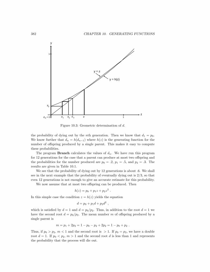
382 CHAPTER 10. GENERATING FUNCTIONS
y = z
y = h(z)
y
z
1
p0
0 d = 0 1d d d d 1 2 3
Figure 10.3: Geometric determination of d.
the probability of dying out by the nth generation. Then we know that d1 = p0.We know further that dn = h(dn−1) where h(z) is the generating function for thenumber of offspring produced by a single parent. This makes it easy to computethese probabilities.
The program Branch calculates the values of dn. We have run this programfor 12 generations for the case that a parent can produce at most two offspring andthe probabilities for the number produced are p0 = .2, p1 = .5, and p2 = .3. Theresults are given in Table 10.1.
We see that the probability of dying out by 12 generations is about .6. We shallsee in the next example that the probability of eventually dying out is 2/3, so thateven 12 generations is not enough to give an accurate estimate for this probability.
We now assume that at most two offspring can be produced. Then
h(z) = p0 + p1z + p2z2 .
In this simple case the condition z = h(z) yields the equation
d = p0 + p1d+ p2d2 ,
which is satisfied by d = 1 and d = p0/p2. Thus, in addition to the root d = 1 wehave the second root d = p0/p2. The mean number m of offspring produced by asingle parent is
m = p1 + 2p2 = 1− p0 − p2 + 2p2 = 1− p0 + p2 .
Thus, if p0 > p2, m < 1 and the second root is > 1. If p0 = p2, we have a doubleroot d = 1. If p0 < p2, m > 1 and the second root d is less than 1 and representsthe probability that the process will die out.

10.2. BRANCHING PROCESSES 383
Generation Probability of dying out1 .22 .3123 .3852034 .4371165 .4758796 .5058787 .5297138 .5490359 .564949
10 .57822511 .58941612 .598931
Table 10.1: Probability of dying out.
p0 = .2092p1 = .2584p2 = .2360p3 = .1593p4 = .0828p5 = .0357p6 = .0133p7 = .0042p8 = .0011p9 = .0002p10 = .0000
Table 10.2: Distribution of number of female children.
Example 10.9 Keyfitz6 compiled and analyzed data on the continuation of thefemale family line among Japanese women. His estimates at the basic probabilitydistribution for the number of female children born to Japanese women of ages45–49 in 1960 are given in Table 10.2.
The expected number of girls in a family is then 1.837 so the probability d ofextinction is less than 1. If we run the program Branch, we can estimate that d isin fact only about .324. 2
Distribution of Offspring
So far we have considered only the first of the two problems raised by Galton,namely the probability of extinction. We now consider the second problem, thatis, the distribution of the number Zn of offspring in the nth generation. The exactform of the distribution is not known except in very special cases. We shall see,
6N. Keyfitz, Introduction to the Mathematics of Population, rev. ed. (Reading, PA: AddisonWesley, 1977).

384 CHAPTER 10. GENERATING FUNCTIONS
however, that we can describe the limiting behavior of Zn as n→∞.We first show that the generating function hn(z) of the distribution of Zn can
be obtained from h(z) for any branching process.We recall that the value of the generating function at the value z for any random
variable X can be written as
h(z) = E(zX) = p0 + p1z + p2z2 + · · · .
That is, h(z) is the expected value of an experiment which has outcome zj withprobability pj .
Let Sn = X1 + X2 + · · · + Xn where each Xj has the same integer-valueddistribution (pj) with generating function k(z) = p0 + p1z + p2z
2 + · · · . Let kn(z)be the generating function of Sn. Then using one of the properties of ordinarygenerating functions discussed in Section 10.1, we have
kn(z) = (k(z))n ,
since the Xj ’s are independent and all have the same distribution.Consider now the branching process Zn. Let hn(z) be the generating function
of Zn. Then
hn+1(z) = E(zZn+1)
=∑k
E(zZn+1 |Zn = k)P (Zn = k) .
If Zn = k, then Zn+1 = X1 +X2 + · · ·+Xk where X1, X2, . . . , Xk are independentrandom variables with common generating function h(z). Thus
E(zZn+1 |Zn = k) = E(zX1+X2+···+Xk) = (h(z))k ,
andhn+1(z) =
∑k
(h(z))kP (Zn = k) .
Buthn(z) =
∑k
P (Zn = k)zk .
Thus,hn+1(z) = hn(h(z)) . (10.5)
Hence the generating function for Z2 is h2(z) = h(h(z)), for Z3 is
h3(z) = h(h(h(z))) ,
and so forth. From this we see also that
hn+1(z) = h(hn(z)) . (10.6)
If we differentiate Equation 10.6 and use the chain rule we have
h′n+1(z) = h′(hn(z))h′n(z) .

10.2. BRANCHING PROCESSES 385
Putting z = 1 and using the fact that hn(1) = 1 and h′n(1) = mn = the meannumber of offspring in the n’th generation, we have
mn+1 = m ·mn .
Thus, m2 = m ·m = m2, m3 = m ·m2 = m3, and in general
mn = mn .
Thus, for a branching process with m > 1, the mean number of offspring growsexponentially at a rate m.
Examples
Example 10.10 For the branching process of Example 10.8 we have
h(z) = 1/2 + (1/4)z + (1/4)z2 ,
h2(z) = h(h(z)) = 1/2 + (1/4)[1/2 + (1/4)z + (1/4)z2]
= +(1/4)[1/2 + (1/4)z + (1/4)z2]2
= 11/16 + (1/8)z + (9/64)z2 + (1/32)z3 + (1/64)z4 .
The probabilities for the number of offspring in the second generation agree withthose obtained directly from the tree measure (see Figure 1). 2
It is clear that even in the simple case of at most two offspring, we cannot easilycarry out the calculation of hn(z) by this method. However, there is one specialcase in which this can be done.
Example 10.11 Assume that the probabilities p1, p2, . . . form a geometric series:pk = bck−1, k = 1, 2, . . . , with 0 < b ≤ 1− c and
p0 = 1− p1 − p2 − · · ·= 1− b− bc− bc2 − · · ·= 1− b
1− c .
Then the generating function h(z) for this distribution is
h(z) = p0 + p1z + p2z2 + · · ·
= 1− b
1− c + bz + bcz2 + bc2z3 + · · ·
= 1− b
1− c +bz
1− cz .
From this we find
h′(z) =bcz
(1− cz)2+
b
1− cz =b
(1− cz)2

386 CHAPTER 10. GENERATING FUNCTIONS
andm = h′(1) =
b
(1− c)2.
We know that if m ≤ 1 the process will surely die out and d = 1. To find theprobability d when m > 1 we must find a root d < 1 of the equation
z = h(z) ,
orz = 1− b
1− c +bz
1− cz .
This leads us to a quadratic equation. We know that z = 1 is one solution. Theother is found to be
d =1− b− cc(1− c) .
It is easy to verify that d < 1 just when m > 1.It is possible in this case to find the distribution of Zn. This is done by first
finding the generating function hn(z).7 The result for m 6= 1 is:
hn(z) = 1−mn
[1− dmn − d
]+mn
[1−dmn−d
]2z
1−[mn−1mn−d
]z.
The coefficients of the powers of z give the distribution for Zn:
P (Zn = 0) = 1−mn 1− dmn − d =
d(mn − 1)mn − d
andP (Zn = j) = mn
( 1− dmn − d
)2
·(mn − 1mn − d
)j−1
,
for j ≥ 1. 2
Example 10.12 Let us re-examine the Keyfitz data to see if a distribution of thetype considered in Example 10.11 could reasonably be used as a model for thispopulation. We would have to estimate from the data the parameters b and c forthe formula pk = bck−1. Recall that
m =b
(1− c)2(10.7)
and the probability d that the process dies out is
d =1− b− cc(1− c) . (10.8)
Solving Equation 10.7 and 10.8 for b and c gives
c =m− 1m− d
7T. E. Harris, The Theory of Branching Processes (Berlin: Springer, 1963), p. 9.

10.2. BRANCHING PROCESSES 387
Geometricpj Data Model0 .2092 .18161 .2584 .36662 .2360 .20283 .1593 .11224 .0828 .06215 .0357 .03446 .0133 .01907 .0042 .01058 .0011 .00589 .0002 .0032
10 .0000 .0018
Table 10.3: Comparison of observed and expected frequencies.
and
b = m( 1− dm− d
)2
.
We shall use the value 1.837 for m and .324 for d that we found in the Keyfitzexample. Using these values, we obtain b = .3666 and c = .5533. Note that(1 − c)2 < b < 1 − c, as required. In Table 10.3 we give for comparison theprobabilities p0 through p8 as calculated by the geometric distribution versus theempirical values.
The geometric model tends to favor the larger numbers of offspring but is similarenough to show that this modified geometric distribution might be appropriate touse for studies of this kind.
Recall that if Sn = X1 + X2 + · · · + Xn is the sum of independent randomvariables with the same distribution then the Law of Large Numbers states thatSn/n converges to a constant, namely E(X1). It is natural to ask if there is asimilar limiting theorem for branching processes.
Consider a branching process with Zn representing the number of offspring aftern generations. Then we have seen that the expected value of Zn is mn. Thus we canscale the random variable Zn to have expected value 1 by considering the randomvariable
Wn =Znmn
.
In the theory of branching processes it is proved that this random variable Wn
will tend to a limit as n tends to infinity. However, unlike the case of the Law ofLarge Numbers where this limit is a constant, for a branching process the limitingvalue of the random variables Wn is itself a random variable.
Although we cannot prove this theorem here we can illustrate it by simulation.This requires a little care. When a branching process survives, the number ofoffspring is apt to get very large. If in a given generation there are 1000 offspring,the offspring of the next generation are the result of 1000 chance events, and it willtake a while to simulate these 1000 experiments. However, since the final result is

388 CHAPTER 10. GENERATING FUNCTIONS
5 10 15 20 25
0.5
1
1.5
2
2.5
3
Figure 10.4: Simulation of Zn/mn for the Keyfitz example.
the sum of 1000 independent experiments we can use the Central Limit Theorem toreplace these 1000 experiments by a single experiment with normal density havingthe appropriate mean and variance. The program BranchingSimulation carriesout this process.
We have run this program for the Keyfitz example, carrying out 10 simulationsand graphing the results in Figure 10.4.
The expected number of female offspring per female is 1.837, so that we aregraphing the outcome for the random variables Wn = Zn/(1.837)n. For three ofthe simulations the process died out, which is consistent with the value d = .3 thatwe found for this example. For the other seven simulations the value of Wn tendsto a limiting value which is different for each simulation. 2
Example 10.13 We now examine the random variable Zn more closely for thecase m < 1 (see Example 10.11). Fix a value t > 0; let [tmn] be the integer part oftmn. Then
P (Zn = [tmn]) = mn(1− dmn − d )2(
mn − 1mn − d )[tmn]−1
=1mn
(1− d
1− d/mn)2(
1− 1/mn
1− d/mn)tm
n+a ,
where |a| ≤ 2. Thus, as n→∞,
mnP (Zn = [tmn])→ (1− d)2 e−t
e−td= (1− d)2e−t(1−d) .
For t = 0,P (Zn = 0)→ d .

10.2. BRANCHING PROCESSES 389
We can compare this result with the Central Limit Theorem for sums Sn of integer-valued independent random variables (see Theorem 9.3), which states that if t is aninteger and u = (t− nµ)/
√σ2n, then as n→∞,
√σ2nP (Sn = u
√σ2n+ µn)→ 1√
2πe−u
2/2 .
We see that the form of these statements are quite similar. It is possible to provea limit theorem for a general class of branching processes that states that undersuitable hypotheses, as n→∞,
mnP (Zn = [tmn])→ k(t) ,
for t > 0, andP (Zn = 0)→ d .
However, unlike the Central Limit Theorem for sums of independent random vari-ables, the function k(t) will depend upon the basic distribution that determines theprocess. Its form is known for only a very few examples similar to the one we haveconsidered here. 2
Chain Letter Problem
Example 10.14 An interesting example of a branching process was suggested byFree Huizinga.8 In 1978, a chain letter called the “Circle of Gold,” believed to havestarted in California, found its way across the country to the theater district of NewYork. The chain required a participant to buy a letter containing a list of 12 namesfor 100 dollars. The buyer gives 50 dollars to the person from whom the letter waspurchased and then sends 50 dollars to the person whose name is at the top of thelist. The buyer then crosses off the name at the top of the list and adds her ownname at the bottom in each letter before it is sold again.
Let us first assume that the buyer may sell the letter only to a single person.If you buy the letter you will want to compute your expected winnings. (We areignoring here the fact that the passing on of chain letters through the mail is afederal offense with certain obvious resulting penalties.) Assume that each personinvolved has a probability p of selling the letter. Then you will receive 50 dollarswith probability p and another 50 dollars if the letter is sold to 12 people, since thenyour name would have risen to the top of the list. This occurs with probability p12,and so your expected winnings are −100 + 50p + 50p12. Thus the chain in thissituation is a highly unfavorable game.
It would be more reasonable to allow each person involved to make a copy ofthe list and try to sell the letter to at least 2 other people. Then you would havea chance of recovering your 100 dollars on these sales, and if any of the letters issold 12 times you will receive a bonus of 50 dollars for each of these cases. We canconsider this as a branching process with 12 generations. The members of the first
8Private communication.

390 CHAPTER 10. GENERATING FUNCTIONS
generation are the letters you sell. The second generation consists of the letters soldby members of the first generation, and so forth.
Let us assume that the probabilities that each individual sells letters to 0, 1,or 2 others are p0, p1, and p2, respectively. Let Z1, Z2, . . . , Z12 be the number ofletters in the first 12 generations of this branching process. Then your expectedwinnings are
50(E(Z1) + E(Z12)) = 50m+ 50m12 ,
where m = p1 +2p2 is the expected number of letters you sold. Thus to be favorablewe just have
50m+ 50m12 > 100 ,
orm+m12 > 2 .
But this will be true if and only if m > 1. We have seen that this will occur inthe quadratic case if and only if p2 > p0. Let us assume for example that p0 = .2,p1 = .5, and p2 = .3. Then m = 1.1 and the chain would be a favorable game. Yourexpected profit would be
50(1.1 + 1.112)− 100 ≈ 112 .
The probability that you receive at least one payment from the 12th generation is1−d12. We find from our program Branch that d12 = .599. Thus, 1−d12 = .401 isthe probability that you receive some bonus. The maximum that you could receivefrom the chain would be 50(2 + 212) = 204,900 if everyone were to successfully selltwo letters. Of course you can not always expect to be so lucky. (What is theprobability of this happening?)
To simulate this game, we need only simulate a branching process for 12 gen-erations. Using a slightly modified version of our program BranchingSimulationwe carried out twenty such simulations, giving the results shown in Table 10.4.
Note that we were quite lucky on a few runs, but we came out ahead only alittle less than half the time. The process died out by the twelfth generation in 12out of the 20 experiments, in good agreement with the probability d12 = .599 thatwe calculated using the program Branch.
Let us modify the assumptions about our chain letter to let the buyer sell theletter to as many people as she can instead of to a maximum of two. We shallassume, in fact, that a person has a large number N of acquaintances and a smallprobability p of persuading any one of them to buy the letter. Then the distributionfor the number of letters that she sells will be a binomial distribution with meanm = Np. Since N is large and p is small, we can assume that the probability pjthat an individual sells the letter to j people is given by the Poisson distribution
pj =e−mmj
j!.

10.2. BRANCHING PROCESSES 391
Z1 Z2 Z3 Z4 Z5 Z6 Z7 Z8 Z9 Z10 Z11 Z12 Profit1 0 0 0 0 0 0 0 0 0 0 0 -501 1 2 3 2 3 2 1 2 3 3 6 2500 0 0 0 0 0 0 0 0 0 0 0 -1002 4 4 2 3 4 4 3 2 2 1 1 501 2 3 5 4 3 3 3 5 8 6 6 2500 0 0 0 0 0 0 0 0 0 0 0 -1002 3 2 2 2 1 2 3 3 3 4 6 3001 2 1 1 1 1 2 1 0 0 0 0 -500 0 0 0 0 0 0 0 0 0 0 0 -1001 0 0 0 0 0 0 0 0 0 0 0 -502 3 2 3 3 3 5 9 12 12 13 15 7501 1 1 0 0 0 0 0 0 0 0 0 -501 2 2 3 3 0 0 0 0 0 0 0 -501 1 1 1 2 2 3 4 4 6 4 5 2001 1 0 0 0 0 0 0 0 0 0 0 -501 0 0 0 0 0 0 0 0 0 0 0 -501 0 0 0 0 0 0 0 0 0 0 0 -501 1 2 3 3 4 2 3 3 3 3 2 501 2 4 6 6 9 10 13 16 17 15 18 8501 0 0 0 0 0 0 0 0 0 0 0 -50
Table 10.4: Simulation of chain letter (finite distribution case).

392 CHAPTER 10. GENERATING FUNCTIONS
Z1 Z2 Z3 Z4 Z5 Z6 Z7 Z8 Z9 Z10 Z11 Z12 Profit1 2 6 7 7 8 11 9 7 6 6 5 2001 0 0 0 0 0 0 0 0 0 0 0 -501 0 0 0 0 0 0 0 0 0 0 0 -501 1 1 0 0 0 0 0 0 0 0 0 -500 0 0 0 0 0 0 0 0 0 0 0 -1001 1 1 1 1 1 2 4 9 7 9 7 3002 3 3 4 2 0 0 0 0 0 0 0 01 0 0 0 0 0 0 0 0 0 0 0 -502 1 0 0 0 0 0 0 0 0 0 0 03 3 4 7 11 17 14 11 11 10 16 25 13000 0 0 0 0 0 0 0 0 0 0 0 -1001 2 2 1 1 3 1 0 0 0 0 0 -500 0 0 0 0 0 0 0 0 0 0 0 -1002 3 1 0 0 0 0 0 0 0 0 0 03 1 0 0 0 0 0 0 0 0 0 0 501 0 0 0 0 0 0 0 0 0 0 0 -503 4 4 7 10 11 9 11 12 14 13 10 5501 3 3 4 9 5 7 9 8 8 6 3 1001 0 4 6 6 9 10 13 0 0 0 0 -501 0 0 0 0 0 0 0 0 0 0 0 -50
Table 10.5: Simulation of chain letter (Poisson case).
The generating function for the Poisson distribution is
h(z) =∞∑j=0
e−mmjzj
j!
= e−m∞∑j=0
mjzj
j!
= e−memz = em(z−1) .
The expected number of letters that an individual passes on is m, and again tobe favorable we must have m > 1. Let us assume again that m = 1.1. Then wecan find again the probability 1− d12 of a bonus from Branch. The result is .232.Although the expected winnings are the same, the variance is larger in this case,and the buyer has a better chance for a reasonably large profit. We again carriedout 20 simulations using the Poisson distribution with mean 1.1. The results areshown in Table 10.5.
We note that, as before, we came out ahead less than half the time, but we alsohad one large profit. In only 6 of the 20 cases did we receive any profit. This isagain in reasonable agreement with our calculation of a probability .232 for thishappening. 2

10.2. BRANCHING PROCESSES 393
Exercises
1 Let Z1, Z2, . . . , ZN describe a branching process in which each parent hasj offspring with probability pj . Find the probability d that the process even-tually dies out if
(a) p0 = 1/2, p1 = 1/4, and p2 = 1/4.
(b) p0 = 1/3, p1 = 1/3, and p2 = 1/3.
(c) p0 = 1/3, p1 = 0, and p2 = 2/3.
(d) pj = 1/2j+1, for j = 0, 1, 2, . . . .
(e) pj = (1/3)(2/3)j , for j = 0, 1, 2, . . . .
(f) pj = e−22j/j!, for j = 0, 1, 2, . . . (estimate d numerically).
2 Let Z1, Z2, . . . , ZN describe a branching process in which each parent hasj offspring with probability pj . Find the probability d that the process diesout if
(a) p0 = 1/2, p1 = p2 = 0, and p3 = 1/2.
(b) p0 = p1 = p2 = p3 = 1/4.
(c) p0 = t, p1 = 1− 2t, p2 = 0, and p3 = t, where t ≤ 1/2.
3 In the chain letter problem (see Example 10.14) find your expected profit if
(a) p0 = 1/2, p1 = 0, and p2 = 1/2.
(b) p0 = 1/6, p1 = 1/2, and p2 = 1/3.
Show that if p0 > 1/2, you cannot expect to make a profit.
4 Let SN = X1 + X2 + · · · + XN , where the Xi’s are independent randomvariables with common distribution having generating function f(z). Assumethat N is an integer valued random variable independent of all of the Xj andhaving generating function g(z). Show that the generating function for SN ish(z) = g(f(z)). Hint : Use the fact that
h(z) = E(zSN ) =∑k
E(zSN |N = k)P (N = k) .
5 We have seen that if the generating function for the offspring of a singleparent is f(z), then the generating function for the number of offspring aftertwo generations is given by h(z) = f(f(z)). Explain how this follows from theresult of Exercise 4.
6 Consider a queueing process (see Example 5.7) such that in each minute either0 or 1 customers arrive with probabilities p or q = 1 − p, respectively. (Thenumber p is called the arrival rate.) When a customer starts service shefinishes in the next minute with probability r. The number r is called theservice rate.) Thus when a customer begins being served she will finish beingserved in j minutes with probability (1− r)j−1r, for j = 1, 2, 3, . . . .

394 CHAPTER 10. GENERATING FUNCTIONS
(a) Find the generating function f(z) for the number of customers who arrivein one minute and the generating function g(z) for the length of time thata person spends in service once she begins service.
(b) Consider a customer branching process by considering the offspring of acustomer to be the customers who arrive while she is being served. UsingExercise 4, show that the generating function for our customer branchingprocess is h(z) = g(f(z)).
(c) If we start the branching process with the arrival of the first customer,then the length of time until the branching process dies out will be thebusy period for the server. Find a condition in terms of the arrival rateand service rate that will assure that the server will ultimately have atime when he is not busy.
7 Let N be the expected total number of offspring in a branching process. Letm be the mean number of offspring of a single parent. Show that
N = 1 +(∑
pk · k)N = 1 +mN
and hence that N is finite if and only if m < 1 and in that case N = 1/(1−m).
8 Consider a branching process such that the number of offspring of a parent isj with probability 1/2j+1 for j = 0, 1, 2, . . . .
(a) Using the results of Example 10.11 show that the probability that thereare j offspring in the nth generation is
p(n)j =
1n(n+1) ( n
n+1 )j , if j ≥ 1,nn+1 , if j = 0.
(b) Show that the probability that the process dies out exactly at the nthgeneration is 1/n(n+ 1).
(c) Show that the expected lifetime is infinite even though d = 1.
10.3 Generating Functions for Continuous Densi-ties
In the previous section, we introduced the concepts of moments and moment gen-erating functions for discrete random variables. These concepts have natural ana-logues for continuous random variables, provided some care is taken in argumentsinvolving convergence.
Moments
If X is a continuous random variable defined on the probability space Ω, withdensity function fX , then we define the nth moment of X by the formula
µn = E(Xn) =∫ +∞
−∞xnfX(x) dx ,

10.3. CONTINUOUS DENSITIES 395
provided the integral
µn = E(Xn) =∫ +∞
−∞|x|nfX(x) dx ,
is finite. Then, just as in the discrete case, we see that µ0 = 1, µ1 = µ, andµ2 − µ2
1 = σ2.
Moment Generating Functions
Now we define the moment generating function g(t) for X by the formula
g(t) =∞∑k=0
µktk
k!=∞∑k=0
E(Xk)tk
k!
= E(etX) =∫ +∞
−∞etxfX(x) dx ,
provided this series converges. Then, as before, we have
µn = g(n)(0) .
Examples
Example 10.15 Let X be a continuous random variable with range [0, 1] anddensity function fX(x) = 1 for 0 ≤ x ≤ 1 (uniform density). Then
µn =∫ 1
0
xn dx =1
n+ 1,
and
g(t) =∞∑k=0
tk
(k + 1)!
=et − 1t
.
Here the series converges for all t. Alternatively, we have
g(t) =∫ +∞
−∞etxfX(x) dx
=∫ 1
0
etx dx =et − 1t
.
Then (by L’Hopital’s rule)
µ0 = g(0) = limt→0
et − 1t
= 1 ,
µ1 = g′(0) = limt→0
tet − et + 1t2
=12,
µ2 = g′′(0) = limt→0
t3et − 2t2et + 2tet − 2tt4
=13.
396 CHAPTER 10. GENERATING FUNCTIONS
In particular, we verify that µ = g′(0) = 1/2 and
σ2 = g′′(0)− (g′(0))2 =13− 1
4=
112
as before (see Example 6.25). 2
Example 10.16 Let X have range [ 0,∞) and density function fX(x) = λe−λx
(exponential density with parameter λ). In this case
µn =∫ ∞
0
xnλe−λx dx = λ(−1)ndn
dλn
∫ ∞0
e−λx dx
= λ(−1)ndn
dλn[1λ
] =n!λn
,
and
g(t) =∞∑k=0
µktk
k!
=∞∑k=0
[t
λ]k =
λ
λ− t .
Here the series converges only for |t| < λ. Alternatively, we have
g(t) =∫ ∞
0
etxλe−λx dx
=λe(t−λ)x
t− λ
∣∣∣∣∞0
=λ
λ− t .
Now we can verify directly that
µn = g(n)(0) =λn!
(λ− t)n+1
∣∣∣∣t=0
=n!λn
.
2
Example 10.17 Let X have range (−∞,+∞) and density function
fX(x) =1√2πe−x
2/2
(normal density). In this case we have
µn =1√2π
∫ +∞
−∞xne−x
2/2 dx
=
(2m)!2mm! , if n = 2m,0, if n = 2m+ 1.
10.3. CONTINUOUS DENSITIES 397
(These moments are calculated by integrating once by parts to show that µn =(n− 1)µn−2, and observing that µ0 = 1 and µ1 = 0.) Hence,
g(t) =∞∑n=0
µntn
n!
=∞∑m=0
t2m
2mm!= et
2/2 .
This series converges for all values of t. Again we can verify that g(n)(0) = µn.Let X be a normal random variable with parameters µ and σ. It is easy to show
that the moment generating function of X is given by
etµ+(σ2/2)t2 .
Now suppose that X and Y are two independent normal random variables withparameters µ1, σ1, and µ2, σ2, respectively. Then, the product of the momentgenerating functions of X and Y is
et(µ1+µ2)+((σ21+σ2
2)/2)t2 .
This is the moment generating function for a normal random variable with meanµ1 + µ2 and variance σ2
1 + σ22 . Thus, the sum of two independent normal random
variables is again normal. (This was proved for the special case that both summandsare standard normal in Example 7.5.) 2
In general, the series defining g(t) will not converge for all t. But in the importantspecial case where X is bounded (i.e., where the range of X is contained in a finiteinterval), we can show that the series does converge for all t.
Theorem 10.4 Suppose X is a continuous random variable with range containedin the interval [−M,M ]. Then the series
g(t) =∞∑k=0
µktk
k!
converges for all t to an infinitely differentiable function g(t), and g(n)(0) = µn.
Proof. We have
µk =∫ +M
−MxkfX(x) dx ,
so
|µk| ≤∫ +M
−M|x|kfX(x) dx
≤ Mk
∫ +M
−MfX(x) dx = Mk .

398 CHAPTER 10. GENERATING FUNCTIONS
Hence, for all N we have
N∑k=0
∣∣∣∣µktkk!
∣∣∣∣ ≤ N∑k=0
(M |t|)kk!
≤ eM |t| ,
which shows that the power series converges for all t. We know that the sum of aconvergent power series is always differentiable. 2
Moment Problem
Theorem 10.5 If X is a bounded random variable, then the moment generatingfunction gX(t) of x determines the density function fX(x) uniquely.
Sketch of the Proof. We know that
gX(t) =∞∑k=0
µktk
k!
=∫ +∞
−∞etxf(x) dx .
If we replace t by iτ , where τ is real and i =√−1, then the series converges for
all τ , and we can define the function
kX(τ) = gX(iτ) =∫ +∞
−∞eiτxfX(x) dx .
The function kX(τ) is called the characteristic function of X, and is defined bythe above equation even when the series for gX does not converge. This equationsays that kX is the Fourier transform of fX . It is known that the Fourier transformhas an inverse, given by the formula
fX(x) =1
2π
∫ +∞
−∞e−iτxkX(τ) dτ ,
suitably interpreted.9 Here we see that the characteristic function kX , and hencethe moment generating function gX , determines the density function fX uniquelyunder our hypotheses. 2
Sketch of the Proof of the Central Limit Theorem
With the above result in mind, we can now sketch a proof of the Central LimitTheorem for bounded continuous random variables (see Theorem 9.6). To this end,let X be a continuous random variable with density function fX , mean µ = 0 andvariance σ2 = 1, and moment generating function g(t) defined by its series for all t.
9H. Dym and H. P. McKean, Fourier Series and Integrals (New York: Academic Press, 1972).

10.3. CONTINUOUS DENSITIES 399
Let X1, X2, . . . , Xn be an independent trials process with each Xi having densityfX , and let Sn = X1 +X2 + · · ·+Xn, and S∗n = (Sn − nµ)/
√nσ2 = Sn/
√n. Then
each Xi has moment generating function g(t), and since the Xi are independent,the sum Sn, just as in the discrete case (see Section 10.1), has moment generatingfunction
gn(t) = (g(t))n ,
and the standardized sum S∗n has moment generating function
g∗n(t) =(g
(t√n
))n.
We now show that, as n→∞, g∗n(t)→ et2/2, where et
2/2 is the moment gener-ating function of the normal density n(x) = (1/
√2π)e−x
2/2 (see Example 10.17).To show this, we set u(t) = log g(t), and
u∗n(t) = log g∗n(t)
= n log g(
t√n
)= nu
(t√n
),
and show that u∗n(t)→ t2/2 as n→∞. First we note that
u(0) = log gn(0) = 0 ,
u′(0) =g′(0)g(0)
=µ1
1= 0 ,
u′′(0) =g′′(0)g(0)− (g′(0))2
(g(0))2
=µ2 − µ2
1
1= σ2 = 1 .
Now by using L’Hopital’s rule twice, we get
limn→∞
u∗n(t) = lims→∞
u(t/√s)
s−1
= lims→∞
u′(t/√s)t
2s−1/2
= lims→∞
u′′(
t√s
)t2
2= σ2 t
2
2=t2
2.
Hence, g∗n(t) → et2/2 as n → ∞. Now to complete the proof of the Central Limit
Theorem, we must show that if g∗n(t) → et2/2, then under our hypotheses the
distribution functions F ∗n(x) of the S∗n must converge to the distribution functionF ∗N (x) of the normal variable N ; that is, that
F ∗n(a) = P (S∗n ≤ a)→ 1√2π
∫ a
−∞e−x
2/2 dx ,
and furthermore, that the density functions f∗n(x) of the S∗n must converge to thedensity function for N ; that is, that
f∗n(x)→ 1√2πe−x
2/2 ,

400 CHAPTER 10. GENERATING FUNCTIONS
as n→∞.Since the densities, and hence the distributions, of the S∗n are uniquely deter-
mined by their moment generating functions under our hypotheses, these conclu-sions are certainly plausible, but their proofs involve a detailed examination ofcharacteristic functions and Fourier transforms, and we shall not attempt themhere.
In the same way, we can prove the Central Limit Theorem for bounded discreterandom variables with integer values (see Theorem 9.4). Let X be a discrete randomvariable with density function p(j), mean µ = 0, variance σ2 = 1, and momentgenerating function g(t), and let X1, X2, . . . , Xn form an independent trials processwith common density p. Let Sn = X1 + X2 + · · · + Xn and S∗n = Sn/
√n, with
densities pn and p∗n, and moment generating functions gn(t) and g∗n(t) =(g( t√
n))n
.
Then we haveg∗n(t)→ et
2/2 ,
just as in the continuous case, and this implies in the same way that the distributionfunctions F ∗n(x) converge to the normal distribution; that is, that
F ∗n(a) = P (S∗n ≤ a)→ 1√2π
∫ a
−∞e−x
2/2 dx ,
as n→∞.The corresponding statement about the distribution functions p∗n, however, re-
quires a little extra care (see Theorem 9.3). The trouble arises because the dis-tribution p(x) is not defined for all x, but only for integer x. It follows that thedistribution p∗n(x) is defined only for x of the form j/
√n, and these values change
as n changes.We can fix this, however, by introducing the function p(x), defined by the for-
mula
p(x) =p(j), if j − 1/2 ≤ x < j + 1/2,0 , otherwise.
Then p(x) is defined for all x, p(j) = p(j), and the graph of p(x) is the step functionfor the distribution p(j) (see Figure 3 of Section 9.1).
In the same way we introduce the step function pn(x) and p∗n(x) associated withthe distributions pn and p∗n, and their moment generating functions gn(t) and g∗n(t).If we can show that g∗n(t)→ et
2/2, then we can conclude that
p∗n(x)→ 1√2πet
2/2 ,
as n→∞, for all x, a conclusion strongly suggested by Figure 9.3.Now g(t) is given by
g(t) =∫ +∞
−∞etxp(x) dx
=+N∑j=−N
∫ j+1/2
j−1/2
etxp(j) dx

10.3. CONTINUOUS DENSITIES 401
=+N∑j=−N
p(j)etjet/2 − e−t/2
2t/2
= g(t)sinh(t/2)t/2
,
where we have put
sinh(t/2) =et/2 − e−t/2
2.
In the same way, we find that
gn(t) = gn(t)sinh(t/2)t/2
,
g∗n(t) = g∗n(t)sinh(t/2
√n)
t/2√n
.
Now, as n→∞, we know that g∗n(t)→ et2/2, and, by L’Hopital’s rule,
limn→∞
sinh(t/2√n)
t/2√n
= 1 .
It follows thatg∗n(t)→ et
2/2 ,
and hence thatp∗n(x)→ 1√
2πe−x
2/2 ,
as n → ∞. The astute reader will note that in this sketch of the proof of Theo-rem 9.3, we never made use of the hypothesis that the greatest common divisor ofthe differences of all the values that the Xi can take on is 1. This is a technicalpoint that we choose to ignore. A complete proof may be found in Gnedenko andKolmogorov.10
Cauchy Density
The characteristic function of a continuous density is a useful tool even in cases whenthe moment series does not converge, or even in cases when the moments themselvesare not finite. As an example, consider the Cauchy density with parameter a = 1(see Example 5.10)
f(x) =1
π(1 + x2).
If X and Y are independent random variables with Cauchy density f(x), then theaverage Z = (X + Y )/2 also has Cauchy density f(x), that is,
fZ(x) = f(x) .
10B. V. Gnedenko and A. N. Kolomogorov, Limit Distributions for Sums of Independent RandomVariables (Reading: Addison-Wesley, 1968), p. 233.

402 CHAPTER 10. GENERATING FUNCTIONS
This is hard to check directly, but easy to check by using characteristic functions.Note first that
µ2 = E(X2) =∫ +∞
−∞
x2
π(1 + x2)dx =∞
so that µ2 is infinite. Nevertheless, we can define the characteristic function kX(τ)of x by the formula
kX(τ) =∫ +∞
−∞eiτx
1π(1 + x2)
dx .
This integral is easy to do by contour methods, and gives us
kX(τ) = kY (τ) = e−|τ | .
Hence,kX+Y (τ) = (e−|τ |)2 = e−2|τ | ,
and sincekZ(τ) = kX+Y (τ/2) ,
we havekZ(τ) = e−2|τ/2| = e−|τ | .
This shows that kZ = kX = kY , and leads to the conclusions that fZ = fX = fY .It follows from this that if X1, X2, . . . , Xn is an independent trials process with
common Cauchy density, and if
An =X1 +X2 + · · ·+Xn
n
is the average of the Xi, then An has the same density as do the Xi. This meansthat the Law of Large Numbers fails for this process; the distribution of the averageAn is exactly the same as for the individual terms. Our proof of the Law of LargeNumbers fails in this case because the variance of Xi is not finite.
Exercises
1 Let X be a continuous random variable with values in [ 0, 2] and density fX .Find the moment generating function g(t) for X if
(a) fX(x) = 1/2.
(b) fX(x) = (1/2)x.
(c) fX(x) = 1− (1/2)x.
(d) fX(x) = |1− x|.(e) fX(x) = (3/8)x2.
Hint : Use the integral definition, as in Examples 10.15 and 10.16.
2 For each of the densities in Exercise 1 calculate the first and second moments,µ1 and µ2, directly from their definition and verify that g(0) = 1, g′(0) = µ1,and g′′(0) = µ2.

10.3. CONTINUOUS DENSITIES 403
3 Let X be a continuous random variable with values in [ 0,∞) and density fX .Find the moment generating functions for X if
(a) fX(x) = 2e−2x.
(b) fX(x) = e−2x + (1/2)e−x.
(c) fX(x) = 4xe−2x.
(d) fX(x) = λ(λx)n−1e−λx/(n− 1)!.
4 For each of the densities in Exercise 3, calculate the first and second moments,µ1 and µ2, directly from their definition and verify that g(0) = 1, g′(0) = µ1,and g′′(0) = µ2.
5 Find the characteristic function kX(τ) for each of the random variables X ofExercise 1.
6 Let X be a continuous random variable whose characteristic function kX(τ)is
kX(τ) = e−|τ |, −∞ < τ < +∞ .
Show directly that the density fX of X is
fX(x) =1
π(1 + x2).
7 Let X be a continuous random variable with values in [ 0, 1], uniform densityfunction fX(x) ≡ 1 and moment generating function g(t) = (et − 1)/t. Findin terms of g(t) the moment generating function for
(a) −X.
(b) 1 +X.
(c) 3X.
(d) aX + b.
8 Let X1, X2, . . . , Xn be an independent trials process with uniform density.Find the moment generating function for
(a) X1.
(b) S2 = X1 +X2.
(c) Sn = X1 +X2 + · · ·+Xn.
(d) An = Sn/n.
(e) S∗n = (Sn − nµ)/√nσ2.
9 Let X1, X2, . . . , Xn be an independent trials process with normal density ofmean 1 and variance 2. Find the moment generating function for
(a) X1.
(b) S2 = X1 +X2.

404 CHAPTER 10. GENERATING FUNCTIONS
(c) Sn = X1 +X2 + · · ·+Xn.
(d) An = Sn/n.
(e) S∗n = (Sn − nµ)/√nσ2.
10 Let X1, X2, . . . , Xn be an independent trials process with density
f(x) =12e−|x|, −∞ < x < +∞ .
(a) Find the mean and variance of f(x).
(b) Find the moment generating function for X1, Sn, An, and S∗n.
(c) What can you say about the moment generating function of S∗n as n →∞?
(d) What can you say about the moment generating function of An as n→∞?

Chapter 11
Markov Chains
11.1 Introduction
Most of our study of probability has dealt with independent trials processes. Theseprocesses are the basis of classical probability theory and much of statistics. Wehave discussed two of the principal theorems for these processes: the Law of LargeNumbers and the Central Limit Theorem.
We have seen that when a sequence of chance experiments forms an indepen-dent trials process, the possible outcomes for each experiment are the same andoccur with the same probability. Further, knowledge of the outcomes of the pre-vious experiments does not influence our predictions for the outcomes of the nextexperiment. The distribution for the outcomes of a single experiment is sufficientto construct a tree and a tree measure for a sequence of n experiments, and wecan answer any probability question about these experiments by using this treemeasure.
Modern probability theory studies chance processes for which the knowledgeof previous outcomes influences predictions for future experiments. In principle,when we observe a sequence of chance experiments, all of the past outcomes couldinfluence our predictions for the next experiment. For example, this should be thecase in predicting a student’s grades on a sequence of exams in a course. But toallow this much generality would make it very difficult to prove general results.
In 1907, A. A. Markov began the study of an important new type of chanceprocess. In this process, the outcome of a given experiment can affect the outcomeof the next experiment. This type of process is called a Markov chain.
Specifying a Markov Chain
We describe a Markov chain as follows: We have a set of states, S = s1, s2, . . . , sr.The process starts in one of these states and moves successively from one state toanother. Each move is called a step. If the chain is currently in state si, thenit moves to state sj at the next step with a probability denoted by pij , and thisprobability does not depend upon which states the chain was in before the current
405

406 CHAPTER 11. MARKOV CHAINS
state.The probabilities pij are called transition probabilities. The process can remain
in the state it is in, and this occurs with probability pii. An initial probabilitydistribution, defined on S, specifies the starting state. Usually this is done byspecifying a particular state as the starting state.
R. A. Howard1 provides us with a picturesque description of a Markov chain asa frog jumping on a set of lily pads. The frog starts on one of the pads and thenjumps from lily pad to lily pad with the appropriate transition probabilities.
Example 11.1 According to Kemeny, Snell, and Thompson,2 the Land of Oz isblessed by many things, but not by good weather. They never have two nice daysin a row. If they have a nice day, they are just as likely to have snow as rain thenext day. If they have snow or rain, they have an even chance of having the samethe next day. If there is change from snow or rain, only half of the time is this achange to a nice day. With this information we form a Markov chain as follows.We take as states the kinds of weather R, N, and S. From the above informationwe determine the transition probabilities. These are most conveniently representedin a square array as
P =
R N S
R 1/2 1/4 1/4N 1/2 0 1/2S 1/4 1/4 1/2
.
2
Transition Matrix
The entries in the first row of the matrix P in Example 11.1 represent the proba-bilities for the various kinds of weather following a rainy day. Similarly, the entriesin the second and third rows represent the probabilities for the various kinds ofweather following nice and snowy days, respectively. Such a square array is calledthe matrix of transition probabilities, or the transition matrix .
We consider the question of determining the probability that, given the chain isin state i today, it will be in state j two days from now. We denote this probabilityby p
(2)ij . In Example 11.1, we see that if it is rainy today then the event that it
is snowy two days from now is the disjoint union of the following three events: 1)it is rainy tomorrow and snowy two days from now, 2) it is nice tomorrow andsnowy two days from now, and 3) it is snowy tomorrow and snowy two days fromnow. The probability of the first of these events is the product of the conditionalprobability that it is rainy tomorrow, given that it is rainy today, and the conditionalprobability that it is snowy two days from now, given that it is rainy tomorrow.Using the transition matrix P, we can write this product as p11p13. The other two
1R. A. Howard, Dynamic Probabilistic Systems, vol. 1 (New York: John Wiley and Sons, 1971).2J. G. Kemeny, J. L. Snell, G. L. Thompson, Introduction to Finite Mathematics, 3rd ed.
(Englewood Cliffs, NJ: Prentice-Hall, 1974).

11.1. INTRODUCTION 407
events also have probabilities that can be written as products of entries of P. Thus,we have
p(2)13 = p11p13 + p12p23 + p13p33 .
This equation should remind the reader of a dot product of two vectors; we aredotting the first row of P with the third column of P. This is just what is donein obtaining the 1, 3-entry of the product of P with itself. In general, if a Markovchain has r states, then
p(2)ij =
r∑k=1
pikpkj .
The following general theorem is easy to prove by using the above observation andinduction.
Theorem 11.1 Let P be the transition matrix of a Markov chain. The ijth en-try p
(n)ij of the matrix Pn gives the probability that the Markov chain, starting in
state si, will be in state sj after n steps.
Proof. The proof of this theorem is left as an exercise (Exercise 17). 2
Example 11.2 (Example 11.1 continued) Consider again the weather in the Landof Oz. We know that the powers of the transition matrix give us interesting in-formation about the process as it evolves. We shall be particularly interested inthe state of the chain after a large number of steps. The program MatrixPowerscomputes the powers of P.
We have run the program MatrixPowers for the Land of Oz example to com-pute the successive powers of P from 1 to 6. The results are shown in Table 11.1.We note that after six days our weather predictions are, to three-decimal-place ac-curacy, independent of today’s weather. The probabilities for the three types ofweather, R, N, and S, are .4, .2, and .4 no matter where the chain started. Thisis an example of a type of Markov chain called a regular Markov chain. For thistype of chain, it is true that long-range predictions are independent of the startingstate. Not all chains are regular, but this is an important class of chains that weshall study in detail later. 2
We now consider the long-term behavior of a Markov chain when it starts in astate chosen by a probability distribution on the set of states, which we will call aprobability vector . A probability vector with r components is a row vector whoseentries are non-negative and sum to 1. If u is a probability vector which representsthe initial state of a Markov chain, then we think of the ith component of u asrepresenting the probability that the chain starts in state si.
With this interpretation of random starting states, it is easy to prove the fol-lowing theorem.

408 CHAPTER 11. MARKOV CHAINS
P1 =
Rain Nice Snow
Rain .500 .250 .250Nice .500 .000 .500Snow .250 .250 .500
P2 =
Rain Nice Snow
Rain .438 .188 .375Nice .375 .250 .375Snow .375 .188 .438
P3 =
Rain Nice Snow
Rain .406 .203 .391Nice .406 .188 .406Snow .391 .203 .406
P4 =
Rain Nice Snow
Rain .402 .199 .398Nice .398 .203 .398Snow .398 .199 .402
P5 =
Rain Nice Snow
Rain .400 .200 .399Nice .400 .199 .400Snow .399 .200 .400
P6 =
Rain Nice Snow
Rain .400 .200 .400Nice .400 .200 .400Snow .400 .200 .400
Table 11.1: Powers of the Land of Oz transition matrix.

11.1. INTRODUCTION 409
Theorem 11.2 Let P be the transition matrix of a Markov chain, and let u be theprobability vector which represents the starting distribution. Then the probabilitythat the chain is in state si after n steps is the ith entry in the vector
u(n) = uPn .
Proof. The proof of this theorem is left as an exercise (Exercise 18). 2
We note that if we want to examine the behavior of the chain under the assump-tion that it starts in a certain state si, we simply choose u to be the probabilityvector with ith entry equal to 1 and all other entries equal to 0.
Example 11.3 In the Land of Oz example (Example 11.1) let the initial probabilityvector u equal (1/3, 1/3, 1/3). Then we can calculate the distribution of the statesafter three days using Theorem 11.2 and our previous calculation of P3. We obtain
u(3) = uP3 = ( 1/3, 1/3, 1/3 )
.406 .203 .391.406 .188 .406.391 .203 .406
= ( .401, .188, .401 ) .
2
Examples
The following examples of Markov chains will be used throughout the chapter forexercises.
Example 11.4 The President of the United States tells person A his or her in-tention to run or not to run in the next election. Then A relays the news to B,who in turn relays the message to C, and so forth, always to some new person. Weassume that there is a probability a that a person will change the answer from yesto no when transmitting it to the next person and a probability b that he or shewill change it from no to yes. We choose as states the message, either yes or no.The transition matrix is then
P =( yes no
yes 1− a a
no b 1− b
).
The initial state represents the President’s choice. 2
Example 11.5 Each time a certain horse runs in a three-horse race, he has proba-bility 1/2 of winning, 1/4 of coming in second, and 1/4 of coming in third, indepen-dent of the outcome of any previous race. We have an independent trials process,

410 CHAPTER 11. MARKOV CHAINS
but it can also be considered from the point of view of Markov chain theory. Thetransition matrix is
P =
W P S
W .5 .25 .25P .5 .25 .25S .5 .25 .25
.
2
Example 11.6 In the Dark Ages, Harvard, Dartmouth, and Yale admitted onlymale students. Assume that, at that time, 80 percent of the sons of Harvard menwent to Harvard and the rest went to Yale, 40 percent of the sons of Yale men wentto Yale, and the rest split evenly between Harvard and Dartmouth; and of the sonsof Dartmouth men, 70 percent went to Dartmouth, 20 percent to Harvard, and10 percent to Yale. We form a Markov chain with transition matrix
P =
H Y D
H .8 .2 0Y .3 .4 .3D .2 .1 .7
.
2
Example 11.7 Modify Example 11.6 by assuming that the son of a Harvard manalways went to Harvard. The transition matrix is now
P =
H Y D
H 1 0 0Y .3 .4 .3D .2 .1 .7
.
2
Example 11.8 (Ehrenfest Model) The following is a special case of a model, calledthe Ehrenfest model,3 that has been used to explain diffusion of gases. The generalmodel will be discussed in detail in Section 11.5. We have two urns that, betweenthem, contain four balls. At each step, one of the four balls is chosen at randomand moved from the urn that it is in into the other urn. We choose, as states, thenumber of balls in the first urn. The transition matrix is then
P =
0 1 2 3 40 0 1 0 0 01 1/4 0 3/4 0 02 0 1/2 0 1/2 03 0 0 3/4 0 1/44 0 0 0 1 0
.
2
3P. and T. Ehrenfest, “Uber zwei bekannte Einwande gegen das Boltzmannsche H-Theorem,”Physikalishce Zeitschrift, vol. 8 (1907), pp. 311-314.

11.1. INTRODUCTION 411
Example 11.9 (Gene Model) The simplest type of inheritance of traits in animalsoccurs when a trait is governed by a pair of genes, each of which may be of two types,say G and g. An individual may have a GG combination or Gg (which is geneticallythe same as gG) or gg. Very often the GG and Gg types are indistinguishable inappearance, and then we say that the G gene dominates the g gene. An individualis called dominant if he or she has GG genes, recessive if he or she has gg, andhybrid with a Gg mixture.
In the mating of two animals, the offspring inherits one gene of the pair fromeach parent, and the basic assumption of genetics is that these genes are selected atrandom, independently of each other. This assumption determines the probabilityof occurrence of each type of offspring. The offspring of two purely dominant parentsmust be dominant, of two recessive parents must be recessive, and of one dominantand one recessive parent must be hybrid.
In the mating of a dominant and a hybrid animal, each offspring must get aG gene from the former and has an equal chance of getting G or g from the latter.Hence there is an equal probability for getting a dominant or a hybrid offspring.Again, in the mating of a recessive and a hybrid, there is an even chance for gettingeither a recessive or a hybrid. In the mating of two hybrids, the offspring has anequal chance of getting G or g from each parent. Hence the probabilities are 1/4for GG, 1/2 for Gg, and 1/4 for gg.
Consider a process of continued matings. We start with an individual of knowngenetic character and mate it with a hybrid. We assume that there is at least oneoffspring. An offspring is chosen at random and is mated with a hybrid and thisprocess repeated through a number of generations. The genetic type of the chosenoffspring in successive generations can be represented by a Markov chain. The statesare dominant, hybrid, and recessive, and indicated by GG, Gg, and gg respectively.
The transition probabilities are
P =
GG Gg gg
GG .5 .5 0Gg .25 .5 .25gg 0 .5 .5
.
2
Example 11.10 Modify Example 11.9 as follows: Instead of mating the oldestoffspring with a hybrid, we mate it with a dominant individual. The transitionmatrix is
P =
GG Gg gg
GG 1 0 0Gg .5 .5 0gg 0 1 0
.
2

412 CHAPTER 11. MARKOV CHAINS
Example 11.11 We start with two animals of opposite sex, mate them, select twoof their offspring of opposite sex, and mate those, and so forth. To simplify theexample, we will assume that the trait under consideration is independent of sex.
Here a state is determined by a pair of animals. Hence, the states of our processwill be: s1 = (GG,GG), s2 = (GG,Gg), s3 = (GG, gg), s4 = (Gg,Gg), s5 =(Gg, gg), and s6 = (gg, gg).
We illustrate the calculation of transition probabilities in terms of the state s2.When the process is in this state, one parent has GG genes, the other Gg. Hence,the probability of a dominant offspring is 1/2. Then the probability of transitionto s1 (selection of two dominants) is 1/4, transition to s2 is 1/2, and to s4 is 1/4.The other states are treated the same way. The transition matrix of this chain is:
P1 =
GG,GG GG,Gg GG,gg Gg,Gg Gg,gg gg,ggGG,GG 1.000 .000 .000 .000 .000 .000GG,Gg .250 .500 .000 .250 .000 .000GG,gg .000 .000 .000 1.000 .000 .000Gg,Gg .062 .250 .125 .250 .250 .062Gg,gg .000 .000 .000 .250 .500 .250gg,gg .000 .000 .000 .000 .000 1.000
.
2
Example 11.12 (Stepping Stone Model) Our final example is another examplethat has been used in the study of genetics. It is called the stepping stone model.4
In this model we have an n-by-n array of squares, and each square is initially anyone of k different colors. For each step, a square is chosen at random. This squarethen chooses one of its eight neighbors at random and assumes the color of thatneighbor. To avoid boundary problems, we assume that if a square S is on theleft-hand boundary, say, but not at a corner, it is adjacent to the square T on theright-hand boundary in the same row as S, and S is also adjacent to the squares justabove and below T . A similar assumption is made about squares on the upper andlower boundaries. (These adjacencies are much easier to understand if one imaginesmaking the array into a cylinder by gluing the top and bottom edge together, andthen making the cylinder into a doughnut by gluing the two circular boundariestogether.) With these adjacencies, each square in the array is adjacent to exactlyeight other squares.
A state in this Markov chain is a description of the color of each square. For thisMarkov chain the number of states is kn
2, which for even a small array of squares
is enormous. This is an example of a Markov chain that is easy to simulate butdifficult to analyze in terms of its transition matrix. The program SteppingStonesimulates this chain. We have started with a random initial configuration of twocolors with n = 20 and show the result after the process has run for some time inFigure 11.2.
4S. Sawyer, “Results for The Stepping Stone Model for Migration in Population Genetics,”Annals of Probability, vol. 4 (1979), pp. 699–728.

11.1. INTRODUCTION 413
Figure 11.1: Initial state of the stepping stone model.
Figure 11.2: State of the stepping stone model after 10,000 steps.
This is an example of an absorbing Markov chain. This type of chain will bestudied in Section 11.2. One of the theorems proved in that section, applied tothe present example, implies that with probability 1, the stones will eventually allbe the same color. By watching the program run, you can see that territories areestablished and a battle develops to see which color survives. At any time theprobability that a particular color will win out is equal to the proportion of thearray of this color. You are asked to prove this in Exercise 11.2.32. 2
Exercises
1 It is raining in the Land of Oz. Determine a tree and a tree measure for thenext three days’ weather. Find w(1),w(2), and w(3) and compare with theresults obtained from P, P2, and P3.
2 In Example 11.4, let a = 0 and b = 1/2. Find P, P2, and P3. What wouldPn be? What happens to Pn as n tends to infinity? Interpret this result.
3 In Example 11.5, find P, P2, and P3. What is Pn?

414 CHAPTER 11. MARKOV CHAINS
4 For Example 11.6, find the probability that the grandson of a man from Har-vard went to Harvard.
5 In Example 11.7, find the probability that the grandson of a man from Harvardwent to Harvard.
6 In Example 11.9, assume that we start with a hybrid bred to a hybrid. Findw(1), w(2), and w(3). What would w(n) be?
7 Find the matrices P2, P3, P4, and Pn for the Markov chain determined by
the transition matrix P =(
1 00 1
). Do the same for the transition matrix
P =(
0 11 0
). Interpret what happens in each of these processes.
8 A certain calculating machine uses only the digits 0 and 1. It is supposed totransmit one of these digits through several stages. However, at every stage,there is a probability p that the digit that enters this stage will be changedwhen it leaves and a probability q = 1−p that it won’t. Form a Markov chainto represent the process of transmission by taking as states the digits 0 and 1.What is the matrix of transition probabilities?
9 For the Markov chain in Exercise 8, draw a tree and assign a tree measureassuming that the process begins in state 0 and moves through two stagesof transmission. What is the probability that the machine, after two stages,produces the digit 0 (i.e., the correct digit)? What is the probability that themachine never changed the digit from 0? Now let p = .1. Using the programMatrixPowers, compute the 100th power of the transition matrix. Interpretthe entries of this matrix. Repeat this with p = .2. Why do the 100th powersappear to be the same?
10 Modify the program MatrixPowers so that it prints out the average An ofthe powers Pn, for n = 1 to N . Try your program on the Land of Oz exampleand compare An and Pn.
11 Assume that a man’s profession can be classified as professional, skilled la-borer, or unskilled laborer. Assume that, of the sons of professional men,80 percent are professional, 10 percent are skilled laborers, and 10 percent areunskilled laborers. In the case of sons of skilled laborers, 60 percent are skilledlaborers, 20 percent are professional, and 20 percent are unskilled. Finally, inthe case of unskilled laborers, 50 percent of the sons are unskilled laborers,and 25 percent each are in the other two categories. Assume that every manhas at least one son, and form a Markov chain by following the profession ofa randomly chosen son of a given family through several generations. Set upthe matrix of transition probabilities. Find the probability that a randomlychosen grandson of an unskilled laborer is a professional man.
12 In Exercise 11, we assumed that every man has a son. Assume instead thatthe probability that a man has at least one son is .8. Form a Markov chain

11.2. ABSORBING MARKOV CHAINS 415
with four states. If a man has a son, the probability that this son is in aparticular profession is the same as in Exercise 11. If there is no son, theprocess moves to state four which represents families whose male line has diedout. Find the matrix of transition probabilities and find the probability thata randomly chosen grandson of an unskilled laborer is a professional man.
13 Write a program to compute u(n) given u and P. Use this program tocompute u(10) for the Land of Oz example, with u = (0, 1, 0), and withu = (1/3, 1/3, 1/3).
14 Using the program MatrixPowers, find P1 through P6 for Examples 11.9and 11.10. See if you can predict the long-range probability of finding theprocess in each of the states for these examples.
15 Write a program to simulate the outcomes of a Markov chain after n steps,given the initial starting state and the transition matrix P as data (see Ex-ample 11.12). Keep this program for use in later problems.
16 Modify the program of Exercise 15 so that it keeps track of the proportion oftimes in each state in n steps. Run the modified program for different startingstates for Example 11.1 and Example 11.8. Does the initial state affect theproportion of time spent in each of the states if n is large?
17 Prove Theorem 11.1.
18 Prove Theorem 11.2.
19 Consider the following process. We have two coins, one of which is fair, and theother of which has heads on both sides. We give these two coins to our friend,who chooses one of them at random (each with probability 1/2). During therest of the process, she uses only the coin that she chose. She now proceedsto toss the coin many times, reporting the results. We consider this processto consist solely of what she reports to us.
(a) Given that she reports a head on the nth toss, what is the probabilitythat a head is thrown on the (n+ 1)st toss?
(b) Consider this process as having two states, heads and tails. By computingthe other three transition probabilities analogous to the one in part (a),write down a “transition matrix” for this process.
(c) Now assume that the process is in state “heads” on both the (n − 1)stand the nth toss. Find the probability that a head comes up on the(n+ 1)st toss.
(d) Is this process a Markov chain?
11.2 Absorbing Markov Chains
The subject of Markov chains is best studied by considering special types of Markovchains. The first type that we shall study is called an absorbing Markov chain.

416 CHAPTER 11. MARKOV CHAINS
1 2 30 4
1 11/2 1/2 1/2
1/2 1/2 1/2
Figure 11.3: Drunkard’s walk.
Definition 11.1 A state si of a Markov chain is called absorbing if it is impossibleto leave it (i.e., pii = 1). A Markov chain is absorbing if it has at least one absorbingstate, and if from every state it is possible to go to an absorbing state (not necessarilyin one step). 2
Definition 11.2 In an absorbing Markov chain, a state which is not absorbing iscalled transient. 2
Drunkard’s Walk
Example 11.13 A man walks along a four-block stretch of Park Avenue (see Fig-ure 11.3). If he is at corner 1, 2, or 3, then he walks to the left or right with equalprobability. He continues until he reaches corner 4, which is a bar, or corner 0,which is his home. If he reaches either home or the bar, he stays there.
We form a Markov chain with states 0, 1, 2, 3, and 4. States 0 and 4 areabsorbing states. The transition matrix is then
P =
0 1 2 3 40 1 0 0 0 01 1/2 0 1/2 0 02 0 1/2 0 1/2 03 0 0 1/2 0 1/24 0 0 0 0 1
.
The states 1, 2, and 3 are transient states, and from any of these it is possible toreach the absorbing states 0 and 4. Hence the chain is an absorbing chain. Whena process reaches an absorbing state, we shall say that it is absorbed . 2
The most obvious question that can be asked about such a chain is: What isthe probability that the process will eventually reach an absorbing state? Otherinteresting questions include: (a) What is the probability that the process will endup in a given absorbing state? (b) On the average, how long will it take for theprocess to be absorbed? (c) On the average, how many times will the process be ineach transient state? The answers to all these questions depend, in general, on thestate from which the process starts as well as the transition probabilities.

11.2. ABSORBING MARKOV CHAINS 417
Canonical Form
Consider an arbitrary absorbing Markov chain. Renumber the states so that thetransient states come first. If there are r absorbing states and t transient states,the transition matrix will have the following canonical form
P =
TR. ABS.
TR. Q R
ABS. 0 I
Here I is an r-by-r indentity matrix, 0 is an r-by-t zero matrix, R is a nonzero
t-by-r matrix, and Q is an t-by-t matrix. The first t states are transient and thelast r states are absorbing.
In Section 11.1, we saw that the entry p(n)ij of the matrix Pn is the probability of
being in the state sj after n steps, when the chain is started in state si. A standardmatrix algebra argument shows that Pn is of the form
Pn =
TR. ABS.
TR. Qn ∗
ABS. 0 I
where the asterisk ∗ stands for the t-by-r matrix in the upper right-hand cornerof Pn. (This submatrix can be written in terms of Q and R, but the expressionis complicated and is not needed at this time.) The form of Pn shows that theentries of Qn give the probabilities for being in each of the transient states after nsteps for each possible transient starting state. For our first theorem we prove thatthe probability of being in the transient states after n steps approaches zero. Thusevery entry of Qn must approach zero as n approaches infinity (i.e, Qn → 0).
In the following, if u and v are two vectors we say that u ≤ v if all componentsof u are less than or equal to the corresponding components of v. Similarly, ifA and B are matrices then A ≤ B if each entry of A is less than or equal to thecorresponding entry of B.
Probability of Absorption
Theorem 11.3 In an absorbing Markov chain, the probability that the processwill be absorbed is 1 (i.e., Qn → 0 as n→∞).
Proof. From each nonabsorbing state sj it is possible to reach an absorbing state.Let mj be the minimum number of steps required to reach an absorbing state,starting from sj . Let pj be the probability that, starting from sj , the process willnot reach an absorbing state in mj steps. Then pj < 1. Let m be the largest of themj and let p be the largest of pj . The probability of not being absorbed in m steps

418 CHAPTER 11. MARKOV CHAINS
is less than or equal to p, in 2n steps less than or equal to p2, etc. Since p < 1 theseprobabilities tend to 0. Since the probability of not being absorbed in n steps ismonotone decreasing, these probabilities also tend to 0, hence limn→∞Qn = 0. 2
The Fundamental Matrix
Theorem 11.4 For an absorbing Markov chain the matrix I − Q has an inverseN and N = I + Q + Q2 + · · · . The ij-entry nij of the matrix N is the expectednumber of times the chain is in state sj , given that it starts in state si. The initialstate is counted if i = j.
Proof. Let (I − Q)x = 0; that is x = Qx. Then, iterating this we see thatx = Qnx. Since Qn → 0, we have Qnx → 0, so x = 0. Thus (I −Q)−1 = Nexists. Note next that
(I−Q)(I + Q + Q2 + · · ·+ Qn) = I−Qn+1 .
Thus multiplying both sides by N gives
I + Q + Q2 + · · ·+ Qn = N(I−Qn+1) .
Letting n tend to infinity we have
N = I + Q + Q2 + · · · .
Let si and sj be two transient states, and assume throughout the remainder ofthe proof that i and j are fixed. Let X(k) be a random variable which equals 1if the chain is in state sj after k steps, and equals 0 otherwise. For each k, thisrandom variable depends upon both i and j; we choose not to explicitly show thisdependence in the interest of clarity. We have
P (X(k) = 1) = q(k)ij ,
andP (X(k) = 0) = 1− q(k)
ij ,
where q(k)ij is the ijth entry of Qk. These equations hold for k = 0 since Q0 = I.
Therefore, since X(k) is a 0-1 random variable, E(X(k)) = q(k)ij .
The expected number of times the chain is in state sj in the first n steps, giventhat it starts in state si, is clearly
E(X(0) +X(1) + · · ·+X(n)
)= q
(0)ij + q
(1)ij + · · ·+ q
(n)ij .
Letting n tend to infinity we have
E(X(0) +X(1) + · · ·
)= q
(0)ij + q
(1)ij + · · · = nij .
2

11.2. ABSORBING MARKOV CHAINS 419
Definition 11.3 For an absorbing Markov chain P, the matrix N = (I−Q)−1 iscalled the fundamental matrix for P. The entry nij of N gives the expected numberof times that the process is in the transient state sj if it is started in the transientstate si. 2
Example 11.14 (Example 11.13 continued) In the Drunkard’s Walk example, thetransition matrix in canonical form is
P =
1 2 3 0 41 0 1/2 0 1/2 02 1/2 0 1/2 0 03 0 1/2 0 0 1/2
0 0 0 0 1 04 0 0 0 0 1
.
From this we see that the matrix Q is
Q =
0 1/2 01/2 0 1/20 1/2 0
,
and
I−Q =
1 −1/2 0−1/2 1 −1/2
0 −1/2 1
.
Computing (I−Q)−1, we find
N = (I−Q)−1 =
1 2 3
1 3/2 1 1/22 1 2 13 1/2 1 3/2
.
From the middle row of N, we see that if we start in state 2, then the expectednumber of times in states 1, 2, and 3 before being absorbed are 1, 2, and 1. 2
Time to Absorption
We now consider the question: Given that the chain starts in state si, what is theexpected number of steps before the chain is absorbed? The answer is given in thenext theorem.
Theorem 11.5 Let ti be the expected number of steps before the chain is absorbed,given that the chain starts in state si, and let t be the column vector whose ithentry is ti. Then
t = Nc ,
where c is a column vector all of whose entries are 1.

420 CHAPTER 11. MARKOV CHAINS
Proof. If we add all the entries in the ith row of N, we will have the expectednumber of times in any of the transient states for a given starting state si, thatis, the expected time required before being absorbed. Thus, ti is the sum of theentries in the ith row of N. If we write this statement in matrix form, we obtainthe theorem. 2
Absorption Probabilities
Theorem 11.6 Let bij be the probability that an absorbing chain will be absorbedin the absorbing state sj if it starts in the transient state si. Let B be the matrixwith entries bij . Then B is an t-by-r matrix, and
B = NR ,
where N is the fundamental matrix and R is as in the canonical form.
Proof. We have
Bij =∑n
∑k
q(n)ik rkj
=∑k
∑n
q(n)ik rkj
=∑k
nikrkj
= (NR)ij .
This completes the proof. 2
Another proof of this is given in Exercise 34.
Example 11.15 (Example 11.14 continued) In the Drunkard’s Walk example, wefound that
N =
1 2 3
1 3/2 1 1/22 1 2 13 1/2 1 3/2
.
Hence,
t = Nc =
3/2 1 1/21 2 1
1/2 1 3/2
111
=
343
.

11.2. ABSORBING MARKOV CHAINS 421
Thus, starting in states 1, 2, and 3, the expected times to absorption are 3, 4, and3, respectively.
From the canonical form,
R =
0 4
1 1/2 02 0 03 0 1/2
.
Hence,
B = NR =
3/2 1 1/21 2 1
1/2 1 3/2
· 1/2 0
0 00 1/2
=
0 4
1 3/4 1/42 1/2 1/23 1/4 3/4
.
Here the first row tells us that, starting from state 1, there is probability 3/4 ofabsorption in state 0 and 1/4 of absorption in state 4. 2
Computation
The fact that we have been able to obtain these three descriptive quantities inmatrix form makes it very easy to write a computer program that determines thesequantities for a given absorbing chain matrix.
The program AbsorbingChain calculates the basic descriptive quantities of anabsorbing Markov chain.
We have run the program AbsorbingChain for the example of the drunkard’swalk (Example 11.13) with 5 blocks. The results are as follows:
Q =
1 2 3 4
1 .00 .50 .00 .002 .50 .00 .50 .003 .00 .50 .00 .504 .00 .00 .50 .00
;
R =
0 5
1 .50 .002 .00 .003 .00 .004 .00 .50
;

422 CHAPTER 11. MARKOV CHAINS
N =
1 2 3 4
1 1.60 1.20 .80 .402 1.20 2.40 1.60 .803 .80 1.60 2.40 1.204 .40 .80 1.20 1.60
;
t =
1 4.002 6.003 6.004 4.00
;
B =
0 5
1 .80 .202 .60 .403 .40 .604 .20 .80
.
Note that the probability of reaching the bar before reaching home, startingat x, is x/5 (i.e., proportional to the distance of home from the starting point).(See Exercise 24.)
Exercises
1 In Example 11.4, for what values of a and b do we obtain an absorbing Markovchain?
2 Show that Example 11.7 is an absorbing Markov chain.
3 Which of the genetics examples (Examples 11.9, 11.10, and 11.11) are ab-sorbing?
4 Find the fundamental matrix N for Example 11.10.
5 For Example 11.11, verify that the following matrix is the inverse of I − Qand hence is the fundamental matrix N.
N =
8/3 1/6 4/3 2/34/3 4/3 8/3 4/34/3 1/3 8/3 4/32/3 1/6 4/3 8/3
.
Find Nc and NR. Interpret the results.
6 In the Land of Oz example (Example 11.1), change the transition matrix bymaking R an absorbing state. This gives
P =
R N S
R 1 0 0N 1/2 0 1/2S 1/4 1/4 1/2
.

11.2. ABSORBING MARKOV CHAINS 423
Find the fundamental matrix N, and also Nc and NR. Interpret the results.
7 In Example 11.8, make states 0 and 4 into absorbing states. Find the fun-damental matrix N, and also Nc and NR, for the resulting absorbing chain.Interpret the results.
8 In Example 11.13 (Drunkard’s Walk) of this section, assume that the proba-bility of a step to the right is 2/3, and a step to the left is 1/3. Find N, Nc,and NR. Compare these with the results of Example 11.15.
9 A process moves on the integers 1, 2, 3, 4, and 5. It starts at 1 and, on eachsuccessive step, moves to an integer greater than its present position, movingwith equal probability to each of the remaining larger integers. State five isan absorbing state. Find the expected number of steps to reach state five.
10 Using the result of Exercise 9, make a conjecture for the form of the funda-mental matrix if the process moves as in that exercise, except that it nowmoves on the integers from 1 to n. Test your conjecture for several differentvalues of n. Can you conjecture an estimate for the expected number of stepsto reach state n, for large n? (See Exercise 11 for a method of determiningthis expected number of steps.)
*11 Let bk denote the expected number of steps to reach n from n − k, in theprocess described in Exercise 9.
(a) Define b0 = 0. Show that for k > 0, we have
bk = 1 +1k
(bk−1 + bk−2 + · · ·+ b0
).
(b) Letf(x) = b0 + b1x+ b2x
2 + · · · .
Using the recursion in part (a), show that f(x) satisfies the differentialequation
(1− x)2y′ − (1− x)y + 1 = 0 .
(c) Show that the general solution of the differential equation in part (b) is
y =− log(1− x)
1− x +c
1− x ,
where c is a constant.
(d) Use part (c) to show that
bk = 1 +12
+13
+ · · ·+ 1k.
12 Three tanks fight a three-way duel. Tank A has probability 1/2 of destroyingthe tank at which it fires, tank B has probability 1/3 of destroying the tank atwhich it fires, and tank C has probability 1/6 of destroying the tank at which

424 CHAPTER 11. MARKOV CHAINS
it fires. The tanks fire together and each tank fires at the strongest opponentnot yet destroyed. Form a Markov chain by taking as states the subsets of theset of tanks. Find N, Nc, and NR, and interpret your results. Hint : Takeas states ABC, AC, BC, A, B, C, and none, indicating the tanks that couldsurvive starting in state ABC. You can omit AB because this state cannot bereached from ABC.
13 Smith is in jail and has 3 dollars; he can get out on bail if he has 8 dollars.A guard agrees to make a series of bets with him. If Smith bets A dollars,he wins A dollars with probability .4 and loses A dollars with probability .6.Find the probability that he wins 8 dollars before losing all of his money if
(a) he bets 1 dollar each time (timid strategy).
(b) he bets, each time, as much as possible but not more than necessary tobring his fortune up to 8 dollars (bold strategy).
(c) Which strategy gives Smith the better chance of getting out of jail?
14 With the situation in Exercise 13, consider the strategy such that for i < 4,Smith bets min(i, 4− i), and for i ≥ 4, he bets according to the bold strategy,where i is his current fortune. Find the probability that he gets out of jailusing this strategy. How does this probability compare with that obtained forthe bold strategy?
15 Consider the game of tennis when deuce is reached. If a player wins the nextpoint, he has advantage. On the following point, he either wins the game or thegame returns to deuce. Assume that for any point, player A has probability.6 of winning the point and player B has probability .4 of winning the point.
(a) Set this up as a Markov chain with state 1: A wins; 2: B wins; 3:advantage A; 4: deuce; 5: advantage B.
(b) Find the absorption probabilities.
(c) At deuce, find the expected duration of the game and the probabilitythat B will win.
Exercises 16 and 17 concern the inheritance of color-blindness, which is a sex-linked characteristic. There is a pair of genes, g and G, of which the formertends to produce color-blindness, the latter normal vision. The G gene isdominant. But a man has only one gene, and if this is g, he is color-blind. Aman inherits one of his mother’s two genes, while a woman inherits one genefrom each parent. Thus a man may be of type G or g, while a woman may betype GG or Gg or gg. We will study a process of inbreeding similar to thatof Example 11.11 by constructing a Markov chain.
16 List the states of the chain. Hint : There are six. Compute the transitionprobabilities. Find the fundamental matrix N, Nc, and NR.

11.2. ABSORBING MARKOV CHAINS 425
17 Show that in both Example 11.11 and the example just given, the probabilityof absorption in a state having genes of a particular type is equal to theproportion of genes of that type in the starting state. Show that this canbe explained by the fact that a game in which your fortune is the number ofgenes of a particular type in the state of the Markov chain is a fair game.5
18 Assume that a student going to a certain four-year medical school in northernNew England has, each year, a probability q of flunking out, a probability r
of having to repeat the year, and a probability p of moving on to the nextyear (in the fourth year, moving on means graduating).
(a) Form a transition matrix for this process taking as states F, 1, 2, 3, 4,and G where F stands for flunking out and G for graduating, and theother states represent the year of study.
(b) For the case q = .1, r = .2, and p = .7 find the time a beginning studentcan expect to be in the second year. How long should this student expectto be in medical school?
(c) Find the probability that this beginning student will graduate.
19 (E. Brown6) Mary and John are playing the following game: They have athree-card deck marked with the numbers 1, 2, and 3 and a spinner with thenumbers 1, 2, and 3 on it. The game begins by dealing the cards out so thatthe dealer gets one card and the other person gets two. A move in the gameconsists of a spin of the spinner. The person having the card with the numberthat comes up on the spinner hands that card to the other person. The gameends when someone has all the cards.
(a) Set up the transition matrix for this absorbing Markov chain, where thestates correspond to the number of cards that Mary has.
(b) Find the fundamental matrix.
(c) On the average, how many moves will the game last?
(d) If Mary deals, what is the probability that John will win the game?
20 Assume that an experiment has m equally probable outcomes. Show that theexpected number of independent trials before the first occurrence of k consec-utive occurrences of one of these outcomes is (mk − 1)/(m− 1). Hint : Forman absorbing Markov chain with states 1, 2, . . . , k with state i representingthe length of the current run. The expected time until a run of k is 1 morethan the expected time until absorption for the chain started in state 1. It hasbeen found that, in the decimal expansion of pi, starting with the 24,658,601stdigit, there is a run of nine 7’s. What would your result say about the ex-pected number of digits necessary to find such a run if the digits are producedrandomly?
5H. Gonshor, “An Application of Random Walk to a Problem in Population Genetics,” Amer-ican Math Monthly, vol. 94 (1987), pp. 668–671
6Private communication.

426 CHAPTER 11. MARKOV CHAINS
21 (Roberts7) A city is divided into 3 areas 1, 2, and 3. It is estimated thatamounts u1, u2, and u3 of pollution are emitted each day from these threeareas. A fraction qij of the pollution from region i ends up the next day atregion j. A fraction qi = 1−
∑j qij > 0 goes into the atmosphere and escapes.
Let w(n)i be the amount of pollution in area i after n days.
(a) Show that w(n) = u + uQ + · · ·+ uQn−1.
(b) Show that w(n) → w, and show how to compute w from u.
(c) The government wants to limit pollution levels to a prescribed level byprescribing w. Show how to determine the levels of pollution u whichwould result in a prescribed limiting value w.
22 In the Leontief economic model,8 there are n industries 1, 2, . . . , n. Theith industry requires an amount 0 ≤ qij ≤ 1 of goods (in dollar value) fromcompany j to produce 1 dollar’s worth of goods. The outside demand on theindustries, in dollar value, is given by the vector d = (d1, d2, . . . , dn). Let Qbe the matrix with entries qij .
(a) Show that if the industries produce total amounts given by the vectorx = (x1, x2, . . . , xn) then the amounts of goods of each type that theindustries will need just to meet their internal demands is given by thevector xQ.
(b) Show that in order to meet the outside demand d and the internal de-mands the industries must produce total amounts given by a vectorx = (x1, x2, . . . , xn) which satisfies the equation x = xQ + d.
(c) Show that if Q is the Q-matrix for an absorbing Markov chain, then itis possible to meet any outside demand d.
(d) Assume that the row sums of Q are less than or equal to 1. Give aneconomic interpretation of this condition. Form a Markov chain by takingthe states to be the industries and the transition probabilites to be the qij .Add one absorbing state 0. Define
qi0 = 1−∑j
qij .
Show that this chain will be absorbing if every company is either makinga profit or ultimately depends upon a profit-making company.
(e) Define xc to be the gross national product. Find an expression for thegross national product in terms of the demand vector d and the vectort giving the expected time to absorption.
23 A gambler plays a game in which on each play he wins one dollar with prob-ability p and loses one dollar with probability q = 1− p. The Gambler’s Ruin
7F. Roberts, Discrete Mathematical Models (Englewood Cliffs, NJ: Prentice Hall, 1976).8W. W. Leontief, Input-Output Economics (Oxford: Oxford University Press, 1966).

11.2. ABSORBING MARKOV CHAINS 427
problem is the problem of finding the probability wx of winning an amount Tbefore losing everything, starting with state x. Show that this problem maybe considered to be an absorbing Markov chain with states 0, 1, 2, . . . , T with0 and T absorbing states. Suppose that a gambler has probability p = .48of winning on each play. Suppose, in addition, that the gambler starts with50 dollars and that T = 100 dollars. Simulate this game 100 times and seehow often the gambler is ruined. This estimates w50.
24 Show that wx of Exercise 23 satisfies the following conditions:
(a) wx = pwx+1 + qwx−1 for x = 1, 2, . . . , T − 1.
(b) w0 = 0.
(c) wT = 1.
Show that these conditions determine wx. Show that, if p = q = 1/2, then
wx =x
T
satisfies (a), (b), and (c) and hence is the solution. If p 6= q, show that
wx =(q/p)x − 1(q/p)T − 1
satisfies these conditions and hence gives the probability of the gambler win-ning.
25 Write a program to compute the probability wx of Exercise 24 for given valuesof x, p, and T . Study the probability that the gambler will ruin the bank in agame that is only slightly unfavorable, say p = .49, if the bank has significantlymore money than the gambler.
*26 We considered the two examples of the Drunkard’s Walk corresponding to thecases n = 4 and n = 5 blocks (see Example 11.13). Verify that in these twoexamples the expected time to absorption, starting at x, is equal to x(n− x).See if you can prove that this is true in general. Hint : Show that if f(x) isthe expected time to absorption then f(0) = f(n) = 0 and
f(x) = (1/2)f(x− 1) + (1/2)f(x+ 1) + 1
for 0 < x < n. Show that if f1(x) and f2(x) are two solutions, then theirdifference g(x) is a solution of the equation
g(x) = (1/2)g(x− 1) + (1/2)g(x+ 1) .
Also, g(0) = g(n) = 0. Show that it is not possible for g(x) to have a strictmaximum or a strict minimum at the point i, where 1 ≤ i ≤ n− 1. Use thisto show that g(i) = 0 for all i. This shows that there is at most one solution.Then verify that the function f(x) = x(n− x) is a solution.

428 CHAPTER 11. MARKOV CHAINS
27 Consider an absorbing Markov chain with state space S. Let f be a functiondefined on S with the property that
f(i) =∑j∈S
pijf(j) ,
or in vector formf = Pf .
Then f is called a harmonic function for P. If you imagine a game in whichyour fortune is f(i) when you are in state i, then the harmonic conditionmeans that the game is fair in the sense that your expected fortune after onestep is the same as it was before the step.
(a) Show that for f harmonicf = Pnf
for all n.
(b) Show, using (a), that for f harmonic
f = P∞f ,
where
P∞ = limn→∞
Pn =(
0 B0 I
).
(c) Using (b), prove that when you start in a transient state i your expectedfinal fortune ∑
k
bikf(k)
is equal to your starting fortune f(i). In other words, a fair game ona finite state space remains fair to the end. (Fair games in general arecalled martingales. Fair games on infinite state spaces need not remainfair with an unlimited number of plays allowed. For example, considerthe game of Heads or Tails (see Example 1.4). Let Peter start with1 penny and play until he has 2. Then Peter will be sure to end up1 penny ahead.)
28 A coin is tossed repeatedly. We are interested in finding the expected numberof tosses until a particular pattern, say B = HTH, occurs for the first time.If, for example, the outcomes of the tosses are HHTTHTH we say that thepattern B has occurred for the first time after 7 tosses. Let TB be the timeto obtain pattern B for the first time. Li9 gives the following method fordetermining E(TB).
We are in a casino and, before each toss of the coin, a gambler enters, pays1 dollar to play, and bets that the pattern B = HTH will occur on the next
9S-Y. R. Li, “A Martingale Approach to the Study of Occurrence of Sequence Patterns inRepeated Experiments,” Annals of Probability, vol. 8 (1980), pp. 1171–1176.

11.2. ABSORBING MARKOV CHAINS 429
three tosses. If H occurs, he wins 2 dollars and bets this amount that the nextoutcome will be T. If he wins, he wins 4 dollars and bets this amount thatH will come up next time. If he wins, he wins 8 dollars and the pattern hasoccurred. If at any time he loses, he leaves with no winnings.
Let A and B be two patterns. Let AB be the amount the gamblers win whoarrive while the pattern A occurs and bet that B will occur. For example, ifA = HT and B = HTH then AB = 2 + 4 = 6 since the first gambler bet onH and won 2 dollars and then bet on T and won 4 dollars more. The secondgambler bet on H and lost. If A = HH and B = HTH, then AB = 2 since thefirst gambler bet on H and won but then bet on T and lost and the secondgambler bet on H and won. If A = B = HTH then AB = BB = 8 + 2 = 10.
Now for each gambler coming in, the casino takes in 1 dollar. Thus the casinotakes in TB dollars. How much does it pay out? The only gamblers who gooff with any money are those who arrive during the time the pattern B occursand they win the amount BB. But since all the bets made are perfectly fairbets, it seems quite intuitive that the expected amount the casino takes inshould equal the expected amount that it pays out. That is, E(TB) = BB.
Since we have seen that for B = HTH, BB = 10, the expected time to reachthe pattern HTH for the first time is 10. If we had been trying to get thepattern B = HHH, then BB = 8 + 4 + 2 = 14 since all the last three gamblersare paid off in this case. Thus the expected time to get the pattern HHH is 14.To justify this argument, Li used a theorem from the theory of martingales(fair games).
We can obtain these expectations by considering a Markov chain whose statesare the possible initial segments of the sequence HTH; these states are HTH,HT, H, and ∅, where ∅ is the empty set. Then, for this example, the transitionmatrix is
HTH HT H ∅HTH 1 0 0 0HT .5 0 0 .5H 0 .5 .5 0∅ 0 0 .5 .5
,
and if B = HTH, E(TB) is the expected time to absorption for this chainstarted in state ∅.Show, using the associated Markov chain, that the values E(TB) = 10 andE(TB) = 14 are correct for the expected time to reach the patterns HTH andHHH, respectively.
29 We can use the gambling interpretation given in Exercise 28 to find the ex-pected number of tosses required to reach pattern B when we start with pat-tern A. To be a meaningful problem, we assume that pattern A does not havepattern B as a subpattern. Let EA(TB) be the expected time to reach patternB starting with pattern A. We use our gambling scheme and assume that thefirst k coin tosses produced the pattern A. During this time, the gamblers

430 CHAPTER 11. MARKOV CHAINS
made an amount AB. The total amount the gamblers will have made whenthe pattern B occurs is BB. Thus, the amount that the gamblers made afterthe pattern A has occurred is BB - AB. Again by the fair game argument,EA(TB) = BB-AB.
For example, suppose that we start with pattern A = HT and are trying toget the pattern B = HTH. Then we saw in Exercise 28 that AB = 4 and BB= 10 so EA(TB) = BB-AB= 6.
Verify that this gambling interpretation leads to the correct answer for allstarting states in the examples that you worked in Exercise 28.
30 Here is an elegant method due to Guibas and Odlyzko10 to obtain the expectedtime to reach a pattern, say HTH, for the first time. Let f(n) be the numberof sequences of length n which do not have the pattern HTH. Let fp(n) be thenumber of sequences that have the pattern for the first time after n tosses.To each element of f(n), add the pattern HTH. Then divide the resultingsequences into three subsets: the set where HTH occurs for the first time attime n+ 1 (for this, the original sequence must have ended with HT); the setwhere HTH occurs for the first time at time n + 2 (cannot happen for thispattern); and the set where the sequence HTH occurs for the first time at timen+ 3 (the original sequence ended with anything except HT). Doing this, wehave
f(n) = fp(n+ 1) + fp(n+ 3) .
Thus,f(n)2n
=2fp(n+ 1)
2n+1+
23fp(n+ 3)2n+3
.
If T is the time that the pattern occurs for the first time, this equality statesthat
P (T > n) = 2P (T = n+ 1) + 8P (T = n+ 3) .
Show that if you sum this equality over all n you obtain
∞∑n=0
P (T > n) = 2 + 8 = 10 .
Show that for any integer-valued random variable
E(T ) =∞∑n=0
P (T > n) ,
and conclude that E(T ) = 10. Note that this method of proof makes veryclear that E(T ) is, in general, equal to the expected amount the casino paysout and avoids the martingale system theorem used by Li.
10L. J. Guibas and A. M. Odlyzko, “String Overlaps, Pattern Matching, and Non-transitiveGames,” Journal of Combinatorial Theory, Series A, vol. 30 (1981), pp. 183–208.

11.2. ABSORBING MARKOV CHAINS 431
31 In Example 11.11, define f(i) to be the proportion of G genes in state i. Showthat f is a harmonic function (see Exercise 27). Why does this show that theprobability of being absorbed in state (GG,GG) is equal to the proportion ofG genes in the starting state? (See Exercise 17.)
32 Show that the stepping stone model (Example 11.12) is an absorbing Markovchain. Assume that you are playing a game with red and green squares, inwhich your fortune at any time is equal to the proportion of red squares atthat time. Give an argument to show that this is a fair game in the sense thatyour expected winning after each step is just what it was before this step.Hint :Show that for every possible outcome in which your fortune will decrease byone there is another outcome of exactly the same probability where it willincrease by one.
Use this fact and the results of Exercise 27 to show that the probability that aparticular color wins out is equal to the proportion of squares that are initiallyof this color.
33 Consider a random walker who moves on the integers 0, 1, . . . , N , moving onestep to the right with probability p and one step to the left with probabilityq = 1 − p. If the walker ever reaches 0 or N he stays there. (This is theGambler’s Ruin problem of Exercise 23.) If p = q show that the function
f(i) = i
is a harmonic function (see Exercise 27), and if p 6= q then
f(i) =(q
p
)iis a harmonic function. Use this and the result of Exercise 27 to show thatthe probability biN of being absorbed in state N starting in state i is
biN =
iN , if p = q,
( qp )i−1
( qp )N−1, if p 6= q.
For an alternative derivation of these results see Exercise 24.
34 Complete the following alternate proof of Theorem 11.6. Let si be a tran-sient state and sj be an absorbing state. If we compute bij in terms of thepossibilities on the outcome of the first step, then we have the equation
bij = pij +∑k
pikbkj ,
where the summation is carried out over all transient states sk. Write this inmatrix form, and derive from this equation the statement
B = NR .

432 CHAPTER 11. MARKOV CHAINS
35 In Monte Carlo roulette (see Example 6.6), under option (c), there are sixstates (S, W , L, E, P1, and P2). The reader is referred to Figure 6.2, whichcontains a tree for this option. Form a Markov chain for this option, and usethe program AbsorbingChain to find the probabilities that you win, lose, orbreak even for a 1 franc bet on red. Using these probabilities, find the expectedwinnings for this bet. For a more general discussion of Markov chains appliedto roulette, see the article of H. Sagan referred to in Example 6.13.
36 We consider next a game called Penney-ante by its inventor W. Penney.11
There are two players; the first player picks a pattern A of H’s and T’s, andthen the second player, knowing the choice of the first player, picks a differentpattern B. We assume that neither pattern is a subpattern of the other pattern.A coin is tossed a sequence of times, and the player whose pattern comes upfirst is the winner. To analyze the game, we need to find the probability pAthat pattern A will occur before pattern B and the probability pB = 1 − pAthat pattern B occurs before pattern A. To determine these probabilities weuse the results of Exercises 28 and 29. Here you were asked to show that, theexpected time to reach a pattern B for the first time is,
E(TB) = BB ,
and, starting with pattern A, the expected time to reach pattern B is
EA(TB) = BB −AB .
(a) Show that the odds that the first player will win are given by JohnConway’s formula12:
pA1− pA
=pApB
=BB −BAAA−AB .
Hint : Explain why
E(TB) = E(TA or B) + pAEA(TB)
and thusBB = E(TA or B) + pA(BB −AB) .
Interchange A and B to find a similar equation involving the pB . Finally,note that
pA + pB = 1 .
Use these equations to solve for pA and pB .
(b) Assume that both players choose a pattern of the same length k. Showthat, if k = 2, this is a fair game, but, if k = 3, the second player hasan advantage no matter what choice the first player makes. (It has beenshown that, for k ≥ 3, if the first player chooses a1, a2, . . . , ak, thenthe optimal strategy for the second player is of the form b, a1, . . . , ak−1
where b is the better of the two choices H or T.13)11W. Penney, “Problem: Penney-Ante,” Journal of Recreational Math, vol. 2 (1969), p. 241.12M. Gardner, “Mathematical Games,” Scientific American, vol. 10 (1974), pp. 120–125.13Guibas and Odlyzko, op. cit.

11.3. ERGODIC MARKOV CHAINS 433
11.3 Ergodic Markov Chains
A second important kind of Markov chain we shall study in detail is an ergodicMarkov chain, defined as follows.
Definition 11.4 A Markov chain is called an ergodic chain if it is possible to gofrom every state to every state (not necessarily in one move). 2
In many books, ergodic Markov chains are called irreducible.
Definition 11.5 A Markov chain is called a regular chain if some power of thetransition matrix has only positive elements. 2
In other words, for some n, it is possible to go from any state to any state inexactly n steps. It is clear from this definition that every regular chain is ergodic.On the other hand, an ergodic chain is not necessarily regular, as the followingexamples show.
Example 11.16 Let the transition matrix of a Markov chain be defined by
P =( 1 2
1 0 12 1 0
).
Then is clear that it is possible to move from any state to any state, so the chain isergodic. However, if n is odd, then it is not possible to move from state 0 to state0 in n steps, and if n is even, then it is not possible to move from state 0 to state 1in n steps, so the chain is not regular. 2
A more interesting example of an ergodic, non-regular Markov chain is provided bythe Ehrenfest urn model.
Example 11.17 Recall the Ehrenfest urn model (Example 11.8). The transitionmatrix for this example is
P =
0 1 2 3 40 0 1 0 0 01 1/4 0 3/4 0 02 0 1/2 0 1/2 03 0 0 3/4 0 1/44 0 0 0 1 0
.
In this example, if we start in state 0 we will, after any even number of steps, be ineither state 0, 2 or 4, and after any odd number of steps, be in states 1 or 3. Thusthis chain is ergodic but not regular. 2

434 CHAPTER 11. MARKOV CHAINS
Regular Markov Chains
Any transition matrix that has no zeros determines a regular Markov chain. How-ever, it is possible for a regular Markov chain to have a transition matrix that haszeros. The transition matrix of the Land of Oz example of Section 11.1 has pNN = 0but the second power P2 has no zeros, so this is a regular Markov chain.
An example of a nonregular Markov chain is an absorbing chain. For example,let
P =(
1 01/2 1/2
)be the transition matrix of a Markov chain. Then all powers of P will have a 0 inthe upper right-hand corner.
We shall now discuss two important theorems relating to regular chains.
Theorem 11.7 Let P be the transition matrix for a regular chain. Then, as n→∞, the powers Pn approach a limiting matrix W with all rows the same vector w.The vector w is a strictly positive probability vector (i.e., the components are allpositive and they sum to one). 2
In the next section we give two proofs of this fundamental theorem. We givehere the basic idea of the first proof.
We want to show that the powers Pn of a regular transition matrix tend to amatrix with all rows the same. This is the same as showing that Pn converges toa matrix with constant columns. Now the jth column of Pn is Pny where y is acolumn vector with 1 in the jth entry and 0 in the other entries. Thus we need onlyprove that for any column vector y,Pny approaches a constant vector as n tend toinfinity.
Since each row of P is a probability vector, Py replaces y by averages of itscomponents. Here is an example: 1/2 1/4 1/4
1/3 1/3 1/31/3 1/2 0
123
=
1/2 · 1 + 1/4 · 2 + 1/4 · 31/3 · 1 + 1/3 · 2 + 1/3 · 31/3 · 1 + 1/2 · 2 + 0 · 3
=
7/42
3/2
.
The result of the averaging process is to make the components of Py more similarthan those of y. In particular, the maximum component decreases (from 3 to 2)and the minimum component increases (from 1 to 3/2). Our proof will show thatas we do more and more of this averaging to get Pny, the difference between themaximum and minimum component will tend to 0 as n → ∞. This means Pnytends to a constant vector. The ijth entry of Pn, p(n)
ij , is the probability that theprocess will be in state sj after n steps if it starts in state si. If we denote thecommon row of W by w, then Theorem 11.7 states that the probability of beingin sj in the long run is approximately wj , the jth entry of w, and is independentof the starting state.

11.3. ERGODIC MARKOV CHAINS 435
Example 11.18 Recall that for the Land of Oz example of Section 11.1, the sixthpower of the transition matrix P is, to three decimal places,
P6 =
R N S
R .4 .2 .4N .4 .2 .4S .4 .2 .4
.
Thus, to this degree of accuracy, the probability of rain six days after a rainy dayis the same as the probability of rain six days after a nice day, or six days aftera snowy day. Theorem 11.7 predicts that, for large n, the rows of P approach acommon vector. It is interesting that this occurs so soon in our example. 2
Theorem 11.8 Let P be a regular transition matrix, let
W = limn→∞
Pn ,
let w be the common row of W, and let c be the column vector all of whosecomponents are 1. Then
(a) wP = w, and any row vector v such that vP = v is a constant multiple of w.
(b) Pc = c, and any column vector x such that Px = x is a multiple of c.
Proof. To prove part (a), we note that from Theorem 11.7,
Pn →W .
Thus,Pn+1 = Pn ·P→WP .
But Pn+1 →W, and so W = WP, and w = wP.Let v be any vector with vP = v. Then v = vPn, and passing to the limit,
v = vW. Let r be the sum of the components of v. Then it is easily checked thatvW = rw. So, v = rw.
To prove part (b), assume that x = Px. Then x = Pnx, and again passing tothe limit, x = Wx. Since all rows of W are the same, the components of Wx areall equal, so x is a multiple of c. 2
Note that an immediate consequence of Theorem 11.8 is the fact that there isonly one probability vector v such that vP = v.
Fixed Vectors
Definition 11.6 A row vector w with the property wP = w is called a fixed rowvector for P. Similarly, a column vector x such that Px = x is called a fixed columnvector for P. 2

436 CHAPTER 11. MARKOV CHAINS
Thus, the common row of W is the unique vector w which is both a fixed rowvector for P and a probability vector. Theorem 11.8 shows that any fixed row vectorfor P is a multiple of w and any fixed column vector for P is a constant vector.
One can also state Definition 11.6 in terms of eigenvalues and eigenvectors. Afixed row vector is a left eigenvector of the matrix P corresponding to the eigenvalue1. A similar statement can be made about fixed column vectors.
We will now give several different methods for calculating the fixed row vectorw for a regular Markov chain.
Example 11.19 By Theorem 11.7 we can find the limiting vector w for the Landof Oz from the fact that
w1 + w2 + w3 = 1
and
(w1 w2 w3 )
1/2 1/4 1/41/2 0 1/21/4 1/4 1/2
= (w1 w2 w3 ) .
These relations lead to the following four equations in three unknowns:
w1 + w2 + w3 = 1 ,
(1/2)w1 + (1/2)w2 + (1/4)w3 = w1 ,
(1/4)w1 + (1/4)w3 = w2 ,
(1/4)w1 + (1/2)w2 + (1/2)w3 = w3 .
Our theorem guarantees that these equations have a unique solution. If theequations are solved, we obtain the solution
w = ( .4 .2 .4 ) ,
in agreement with that predicted from P6, given in Example 11.2. 2
To calculate the fixed vector, we can assume that the value at a particular state,say state one, is 1, and then use all but one of the linear equations from wP = w.This set of equations will have a unique solution and we can obtain w from thissolution by dividing each of its entries by their sum to give the probability vector w.We will now illustrate this idea for the above example.
Example 11.20 (Example 11.19 continued) We set w1 = 1, and then solve thefirst and second linear equations from wP = w. We have
(1/2) + (1/2)w2 + (1/4)w3 = 1 ,
(1/4) + (1/4)w3 = w2 .
If we solve these, we obtain
(w1 w2 w3 ) = ( 1 1/2 1 ) .
11.3. ERGODIC MARKOV CHAINS 437
Now we divide this vector by the sum of the components, to obtain the final answer:
w = ( .4 .2 .4 ) .
This method can be easily programmed to run on a computer. 2
As mentioned above, we can also think of the fixed row vector w as a lefteigenvector of the transition matrix P. Thus, if we write I to denote the identitymatrix, then w satisfies the matrix equation
wP = wI ,
or equivalently,w(P− I) = 0 .
Thus, w is in the left nullspace of the matrix P − I. Furthermore, Theorem 11.8states that this left nullspace has dimension 1. Certain computer programminglanguages can find nullspaces of matrices. In such languages, one can find the fixedrow probability vector for a matrix P by computing the left nullspace and thennormalizing a vector in the nullspace so the sum of its components is 1.
The program FixedVector uses one of the above methods (depending uponthe language in which it is written) to calculate the fixed row probability vector forregular Markov chains.
So far we have always assumed that we started in a specific state. The followingtheorem generalizes Theorem 11.7 to the case where the starting state is itselfdetermined by a probability vector.
Theorem 11.9 Let P be the transition matrix for a regular chain and v an arbi-trary probability vector. Then
limn→∞
vPn = w ,
where w is the unique fixed probability vector for P.
Proof. By Theorem 11.7,limn→∞
Pn = W .
Hence,limn→∞
vPn = vW .
But the entries in v sum to 1, and each row of W equals w. From these statements,it is easy to check that
vW = w .
2
If we start a Markov chain with initial probabilities given by v, then the proba-bility vector vPn gives the probabilities of being in the various states after n steps.Theorem 11.9 then establishes the fact that, even in this more general class ofprocesses, the probability of being in sj approaches wj .

438 CHAPTER 11. MARKOV CHAINS
Equilibrium
We also obtain a new interpretation for w. Suppose that our starting vector picksstate si as a starting state with probability wi, for all i. Then the probability ofbeing in the various states after n steps is given by wPn = w, and is the same on allsteps. This method of starting provides us with a process that is called “stationary.”The fact that w is the only probability vector for which wP = w shows that wemust have a starting probability vector of exactly the kind described to obtain astationary process.
Many interesting results concerning regular Markov chains depend only on thefact that the chain has a unique fixed probability vector which is positive. Thisproperty holds for all ergodic Markov chains.
Theorem 11.10 For an ergodic Markov chain, there is a unique probability vec-tor w such that wP = w and w is strictly positive. Any row vector such thatvP = v is a multiple of w. Any column vector x such that Px = x is a constantvector.
Proof. This theorem states that Theorem 11.8 is true for ergodic chains. Theresult follows easily from the fact that, if P is an ergodic transition matrix, thenP = (1/2)I + (1/2)P is a regular transition matrix with the same fixed vectors (seeExercises 25–28). 2
For ergodic chains, the fixed probability vector has a slightly different inter-pretation. The following two theorems, which we will not prove here, furnish aninterpretation for this fixed vector.
Theorem 11.11 Let P be the transition matrix for an ergodic chain. Let An bethe matrix defined by
An =I + P + P2 + · · ·+ Pn
n+ 1.
Then An → W, where W is a matrix all of whose rows are equal to the uniquefixed probability vector w for P. 2
If P is the transition matrix of an ergodic chain, then Theorem 11.8 statesthat there is only one fixed row probability vector for P. Thus, we can use thesame techniques that were used for regular chains to solve for this fixed vector. Inparticular, the program FixedVector works for ergodic chains.
To interpret Theorem 11.11, let us assume that we have an ergodic chain thatstarts in state si. Let X(m) = 1 if the mth step is to state sj and 0 otherwise. Thenthe average number of times in state sj in the first n steps is given by
H(n) =X(0) +X(1) +X(2) + · · ·+X(n)
n+ 1.
But X(m) takes on the value 1 with probability p(m)ij and 0 otherwise. Thus
E(X(m)) = p(m)ij , and the ijth entry of An gives the expected value of H(n), that

11.3. ERGODIC MARKOV CHAINS 439
is, the expected proportion of times in state sj in the first n steps if the chain startsin state si.
If we call being in state sj success and any other state failure, we could ask ifa theorem analogous to the law of large numbers for independent trials holds. Theanswer is yes and is given by the following theorem.
Theorem 11.12 (Law of Large Numbers for Ergodic Markov Chains) LetH
(n)j be the proportion of times in n steps that an ergodic chain is in state sj . Then
for any ε > 0,
P(|H(n)
j − wj | > ε)→ 0 ,
independent of the starting state si. 2
We have observed that every regular Markov chain is also an ergodic chain.Hence, Theorems 11.11 and 11.12 apply also for regular chains. For example, thisgives us a new interpretation for the fixed vector w = (.4, .2, .4) in the Land of Ozexample. Theorem 11.11 predicts that, in the long run, it will rain 40 percent ofthe time in the Land of Oz, be nice 20 percent of the time, and snow 40 percent ofthe time.
Simulation
We illustrate Theorem 11.12 by writing a program to simulate the behavior of aMarkov chain. SimulateChain is such a program.
Example 11.21 In the Land of Oz, there are 525 days in a year. We have simulatedthe weather for one year in the Land of Oz, using the program SimulateChain.The results are shown in Table 11.2.
SSRNRNSSSSSSNRSNSSRNSRNSSSNSRRRNSSSNRRSSSSNRSSNSRRRRRRNSSSSSRRRSNSNRRRRSRSRNSNSRRNRRNRSSNSRNRNSSRRSRNSSSNRSRRSSNRSNRRNSSSSNSSNSRSRRNSSNSSRNSSRRNRRRSRNRRRNSSSNRNSRNSNRNRSSSRSSNRSSSNSSSSSSNSSSNSNSRRNRNRRRRSRRRSSSSNRRSSSSRSRRRNRRRSSSSRRNRRRSRSSRRRRSSRNRRRRRRNSSRNRSSSNRNSNRRRRNRRRNRSNRRNSRRSNRRRRSSSRNRRRNSNSSSSSRRRRSRNRSSRRRRSSSRRRNRNRRRSRSRNSNSSRRRRRNSNRNSNRRNRRRRRRSSSNRSSRSNRSSSNSNRNSNSSSNRRSRRRNRRRRNRNRSSSNSRSNRNRRSNRRNSRSSSRNSRRSSNSRRRNRRSNRRNSSSSSNRNSSSSSSSNRNSRRRNSSRRRNSSSNRRSRNSSRRNRRNRSNRRRRRRRRRNSNRRRRRNSRRSSSSNSNS
State Times Fraction
R 217 .413N 109 .208S 199 .379
Table 11.2: Weather in the Land of Oz.

440 CHAPTER 11. MARKOV CHAINS
We note that the simulation gives a proportion of times in each of the states nottoo different from the long run predictions of .4, .2, and .4 assured by Theorem 11.7.To get better results we have to simulate our chain for a longer time. We do thisfor 10,000 days without printing out each day’s weather. The results are shown inTable 11.3. We see that the results are now quite close to the theoretical values of.4, .2, and .4.
State Times Fraction
R 4010 .401N 1902 .19S 4088 .409
Table 11.3: Comparison of observed and predicted frequencies for the Land of Oz.
2
Examples of Ergodic Chains
The computation of the fixed vector w may be difficult if the transition matrixis very large. It is sometimes useful to guess the fixed vector on purely intuitivegrounds. Here is a simple example to illustrate this kind of situation.
Example 11.22 A white rat is put into the maze of Figure 11.4. There are ninecompartments with connections between the compartments as indicated. The ratmoves through the compartments at random. That is, if there are k ways to leavea compartment, it chooses each of these with equal probability. We can representthe travels of the rat by a Markov chain process with transition matrix given by
P =
1 2 3 4 5 6 7 8 91 0 1/2 0 0 0 1/2 0 0 02 1/3 0 1/3 0 1/3 0 0 0 03 0 1/2 0 1/2 0 0 0 0 04 0 0 1/3 0 1/3 0 0 0 1/35 0 1/4 0 1/4 0 1/4 0 1/4 06 1/3 0 0 0 1/3 0 1/3 0 07 0 0 0 0 0 1/2 0 1/2 08 0 0 0 0 1/3 0 1/3 0 1/39 0 0 0 1/2 0 0 0 1/2 0
.
That this chain is not regular can be seen as follows: From an odd-numberedstate the process can go only to an even-numbered state, and from an even-numberedstate it can go only to an odd number. Hence, starting in state i the process willbe alternately in even-numbered and odd-numbered states. Therefore, odd powersof P will have 0’s for the odd-numbered entries in row 1. On the other hand, aglance at the maze shows that it is possible to go from every state to every otherstate, so that the chain is ergodic.

11.3. ERGODIC MARKOV CHAINS 441
1 2 3
456
7 8 9
Figure 11.4: The maze problem.
To find the fixed probability vector for this matrix, we would have to solve tenequations in nine unknowns. However, it would seem reasonable that the timesspent in each compartment should, in the long run, be proportional to the numberof entries to each compartment. Thus, we try the vector whose jth component isthe number of entries to the jth compartment:
x = ( 2 3 2 3 4 3 2 3 2 ) .
It is easy to check that this vector is indeed a fixed vector so that the uniqueprobability vector is this vector normalized to have sum 1:
w = ( 112
18
112
18
16
18
112
18
112 ) .
2
Example 11.23 (Example 11.8 continued) We recall the Ehrenfest urn model ofExample 11.8. The transition matrix for this chain is as follows:
P =
0 1 2 3 40 .000 1.000 .000 .000 .0001 .250 .000 .750 .000 .0002 .000 .500 .000 .500 .0003 .000 .000 .750 .000 .2504 .000 .000 .000 1.000 .000
.
If we run the program FixedVector for this chain, we obtain the vector
w =( 0 1 2 3 4.0625 .2500 .3750 .2500 .0625
).
By Theorem 11.12, we can interpret these values for wi as the proportion of timesthe process is in each of the states in the long run. For example, the proportion of

442 CHAPTER 11. MARKOV CHAINS
times in state 0 is .0625 and the proportion of times in state 1 is .375. The astutereader will note that these numbers are the binomial distribution 1/16, 4/16, 6/16,4/16, 1/16. We could have guessed this answer as follows: If we consider a particularball, it simply moves randomly back and forth between the two urns. This suggeststhat the equilibrium state should be just as if we randomly distributed the fourballs in the two urns. If we did this, the probability that there would be exactlyj balls in one urn would be given by the binomial distribution b(n, p, j) with n = 4and p = 1/2. 2
Exercises
1 Which of the following matrices are transition matrices for regular Markovchains?
(a) P =(.5 .5.5 .5
).
(b) P =(.5 .51 0
).
(c) P =
1/3 0 2/30 1 00 1/5 4/5
.
(d) P =(
0 11 0
).
(e) P =
1/2 1/2 00 1/2 1/2
1/3 1/3 1/3
.
2 Consider the Markov chain with transition matrix
P =
1/2 1/3 1/63/4 0 1/40 1 0
.
(a) Show that this is a regular Markov chain.
(b) The process is started in state 1; find the probability that it is in state 3after two steps.
(c) Find the limiting probability vector w.
3 Consider the Markov chain with general 2× 2 transition matrix
P =(
1− a a
b 1− b
).
(a) Under what conditions is P absorbing?
(b) Under what conditions is P ergodic but not regular?
(c) Under what conditions is P regular?

11.3. ERGODIC MARKOV CHAINS 443
4 Find the fixed probability vector w for the matrices in Exercise 3 that areergodic.
5 Find the fixed probability vector w for each of the following regular matrices.
(a) P =(.75 .25.5 .5
).
(b) P =(.9 .1.1 .9
).
(c) P =
3/4 1/4 00 2/3 1/3
1/4 1/4 1/2
.
6 Consider the Markov chain with transition matrix in Exercise 3, with a = b =1. Show that this chain is ergodic but not regular. Find the fixed probabilityvector and interpret it. Show that Pn does not tend to a limit, but that
An =I + P + P2 + · · ·+ Pn
n+ 1
does.
7 Consider the Markov chain with transition matrix of Exercise 3, with a = 0and b = 1/2. Compute directly the unique fixed probability vector, and useyour result to prove that the chain is not ergodic.
8 Show that the matrix
P =
1 0 01/4 1/2 1/40 0 1
has more than one fixed probability vector. Find the matrix that Pn ap-proaches as n → ∞, and verify that it is not a matrix all of whose rows arethe same.
9 Prove that, if a 3-by-3 transition matrix has the property that its column sumsare 1, then (1/3, 1/3, 1/3) is a fixed probability vector. State a similar resultfor n-by-n transition matrices. Interpret these results for ergodic chains.
10 Is the Markov chain in Example 11.10 ergodic?
11 Is the Markov chain in Example 11.11 ergodic?
12 Consider Example 11.13 (Drunkard’s Walk). Assume that if the walker reachesstate 0, he turns around and returns to state 1 on the next step and, simi-larly, if he reaches 4 he returns on the next step to state 3. Is this new chainergodic? Is it regular?
13 For Example 11.4 when P is ergodic, what is the proportion of people whoare told that the President will run? Interpret the fact that this proportionis independent of the starting state.

444 CHAPTER 11. MARKOV CHAINS
14 Consider an independent trials process to be a Markov chain whose states arethe possible outcomes of the individual trials. What is its fixed probabilityvector? Is the chain always regular? Illustrate this for Example 11.5.
15 Show that Example 11.8 is an ergodic chain, but not a regular chain. Showthat its fixed probability vector w is a binomial distribution.
16 Show that Example 11.9 is regular and find the limiting vector.
17 Toss a fair die repeatedly. Let Sn denote the total of the outcomes throughthe nth toss. Show that there is a limiting value for the proportion of the firstn values of Sn that are divisible by 7, and compute the value for this limit.Hint : The desired limit is an equilibrium probability vector for an appropriateseven state Markov chain.
18 Let P be the transition matrix of a regular Markov chain. Assume that thereare r states and let N(r) be the smallest integer n such that P is regular ifand only if PN(r) has no zero entries. Find a finite upper bound for N(r).See if you can determine N(3) exactly.
*19 Define f(r) to be the smallest integer n such that for all regular Markov chainswith r states, the nth power of the transition matrix has all entries positive.It has been shown,14 that f(r) = r2 − 2r + 2.
(a) Define the transition matrix of an r-state Markov chain as follows: Forstates si, with i = 1, 2, . . . , r−2, P(i, i+1) = 1, P(r−1, r) = P(r−1, 1) =1/2, and P(r, 1) = 1. Show that this is a regular Markov chain.
(b) For r = 3, verify that the fifth power is the first power that has no zeros.
(c) Show that, for general r, the smallest n such that Pn has all entriespositive is n = f(r).
20 A discrete time queueing system of capacity n consists of the person beingserved and those waiting to be served. The queue length x is observed eachsecond. If 0 < x < n, then with probability p, the queue size is increased byone by an arrival and, inependently, with probability r, it is decreased by onebecause the person being served finishes service. If x = 0, only an arrival (withprobability p) is possible. If x = n, an arrival will depart without waiting forservice, and so only the departure (with probability r) of the person beingserved is possible. Form a Markov chain with states given by the number ofcustomers in the queue. Modify the program FixedVector so that you caninput n, p, and r, and the program will construct the transition matrix andcompute the fixed vector. The quantity s = p/r is called the traffic intensity.Describe the differences in the fixed vectors according as s < 1, s = 1, ors > 1.
14E. Seneta, Non-Negative Matrices: An Introduction to Theory and Applications, Wiley, NewYork, 1973, pp. 52-54.

11.3. ERGODIC MARKOV CHAINS 445
21 Write a computer program to simulate the queue in Exercise 20. Have yourprogram keep track of the proportion of the time that the queue length is j forj = 0, 1, . . . , n and the average queue length. Show that the behavior of thequeue length is very different depending upon whether the traffic intensity shas the property s < 1, s = 1, or s > 1.
22 In the queueing problem of Exercise 20, let S be the total service time requiredby a customer and T the time between arrivals of the customers.
(a) Show that P (S = j) = (1 − r)j−1r and P (T = j) = (1 − p)j−1p, forj > 0.
(b) Show that E(S) = 1/r and E(T ) = 1/p.
(c) Interpret the conditions s < 1, s = 1 and s > 1 in terms of these expectedvalues.
23 In Exercise 20 the service time S has a geometric distribution with E(S) =1/r. Assume that the service time is, instead, a constant time of t seconds.Modify your computer program of Exercise 21 so that it simulates a constanttime service distribution. Compare the average queue length for the twotypes of distributions when they have the same expected service time (i.e.,take t = 1/r). Which distribution leads to the longer queues on the average?
24 A certain experiment is believed to be described by a two-state Markov chainwith the transition matrix P, where
P =(.5 .5p 1− p
)and the parameter p is not known. When the experiment is performed manytimes, the chain ends in state one approximately 20 percent of the time and instate two approximately 80 percent of the time. Compute a sensible estimatefor the unknown parameter p and explain how you found it.
25 Prove that, in an r-state ergodic chain, it is possible to go from any state toany other state in at most r − 1 steps.
26 Let P be the transition matrix of an r-state ergodic chain. Prove that, if thediagonal entries pii are positive, then the chain is regular.
27 Prove that if P is the transition matrix of an ergodic chain, then (1/2)(I+P)is the transition matrix of a regular chain. Hint : Use Exercise 26.
28 Prove that P and (1/2)(I + P) have the same fixed vectors.
29 In his book, Wahrscheinlichkeitsrechnung und Statistik,15 A. Engle proposesan algorithm for finding the fixed vector for an ergodic Markov chain whenthe transition probabilities are rational numbers. Here is his algorithm: For
15A. Engle, Wahrscheinlichkeitsrechnung und Statistik, vol. 2 (Stuttgart: Klett Verlag, 1976).

446 CHAPTER 11. MARKOV CHAINS
(4 2 4)(5 2 3)(8 2 4)(7 3 4)(8 4 4)(8 3 5)(8 4 8)(10 4 6)(12 4 8)(12 5 7)(12 6 8)(13 5 8)(16 6 8)(15 6 9)(16 6 12)(17 7 10)(20 8 12)(20 8 12) .
Table 11.4: Distribution of chips.
each state i, let ai be the least common multiple of the denominators of thenon-zero entries in the ith row. Engle describes his algorithm in terms of mov-ing chips around on the states—indeed, for small examples, he recommendsimplementing the algorithm this way. Start by putting ai chips on state i forall i. Then, at each state, redistribute the ai chips, sending aipij to state j.The number of chips at state i after this redistribution need not be a multipleof ai. For each state i, add just enough chips to bring the number of chips atstate i up to a multiple of ai. Then redistribute the chips in the same manner.This process will eventually reach a point where the number of chips at eachstate, after the redistribution, is the same as before redistribution. At thispoint, we have found a fixed vector. Here is an example:
P =
1 2 3
1 1/2 1/4 1/42 1/2 0 1/23 1/2 1/4 1/4
.
We start with a = (4, 2, 4). The chips after successive redistributions areshown in Table 11.4.
We find that a = (20, 8, 12) is a fixed vector.
(a) Write a computer program to implement this algorithm.
(b) Prove that the algorithm will stop. Hint : Let b be a vector with integercomponents that is a fixed vector for P and such that each coordinate of

11.4. FUNDAMENTAL LIMIT THEOREM 447
the starting vector a is less than or equal to the corresponding componentof b. Show that, in the iteration, the components of the vectors arealways increasing, and always less than or equal to the correspondingcomponent of b.
30 (Coffman, Kaduta, and Shepp16) A computing center keeps information on atape in positions of unit length. During each time unit there is one request tooccupy a unit of tape. When this arrives the first free unit is used. Also, duringeach second, each of the units that are occupied is vacated with probability p.Simulate this process, starting with an empty tape. Estimate the expectednumber of sites occupied for a given value of p. If p is small, can you choose thetape long enough so that there is a small probability that a new job will haveto be turned away (i.e., that all the sites are occupied)? Form a Markov chainwith states the number of sites occupied. Modify the program FixedVectorto compute the fixed vector. Use this to check your conjecture by simulation.
*31 (Alternate proof of Theorem 11.8) Let P be the transition matrix of an ergodicMarkov chain. Let x be any column vector such that Px = x. Let M be themaximum value of the components of x. Assume that xi = M . Show that ifpij > 0 then xj = M . Use this to prove that x must be a constant vector.
32 Let P be the transition matrix of an ergodic Markov chain. Let w be a fixedprobability vector (i.e., w is a row vector with wP = w). Show that if wi = 0and pji > 0 then wj = 0. Use this to show that the fixed probability vectorfor an ergodic chain cannot have any 0 entries.
33 Find a Markov chain that is neither absorbing or ergodic.
11.4 Fundamental Limit Theorem for RegularChains
The fundamental limit theorem for regular Markov chains states that if P is aregular transition matrix then
limn→∞
Pn = W ,
where W is a matrix with each row equal to the unique fixed probability row vectorw for P. In this section we shall give two very different proofs of this theorem.
Our first proof is carried out by showing that, for any column vector y, Pnytends to a constant vector. As indicated in Section 11.3, this will show that Pn
converges to a matrix with constant columns or, equivalently, to a matrix with allrows the same.
The following lemma says that if an r-by-r transition matrix has no zero entries,and y is any column vector with r entries, then the vector Py has entries which are“closer together” than the entries are in y.
16E. G. Coffman, J. T. Kaduta, and L. A. Shepp, “On the Asymptotic Optimality of First-Storage Allocation,” IEEE Trans. Software Engineering, vol. II (1985), pp. 235-239.

448 CHAPTER 11. MARKOV CHAINS
Lemma 11.1 Let P be an r-by-r transition matrix with no zero entries. Let d bethe smallest entry of the matrix. Let y be a column vector with r components, thelargest of which is M0 and the smallest m0. Let M1 and m1 be the largest andsmallest component, respectively, of the vector Py. Then
M1 −m1 ≤ (1− 2d)(M0 −m0) .
Proof. In the discussion following Theorem11.7, it was noted that each entry in thevector Py is a weighted average of the entries in y. The largest weighted averagethat could be obtained in the present case would occur if all but one of the entriesof y have value M0 and one entry has value m0, and this one small entry is weightedby the smallest possible weight, namely d. In this case, the weighted average wouldequal
dm0 + (1− d)M0 .
Similarly, the smallest possible weighted average equals
dM0 + (1− d)m0 .
Thus,
M1 −m1 ≤(dm0 + (1− d)M0
)−(dM0 + (1− d)m0
)= (1− 2d)(M0 −m0) .
This completes the proof of the lemma. 2
We turn now to the proof of the fundamental limit theorem for regular Markovchains.
Theorem 11.13 (Fundamental Limit Theorem for Regular Chains) If P isthe transition matrix for a regular Markov chain, then
limn→∞
Pn = W ,
where W is matrix with all rows equal. Furthermore, all entries in W are strictlypositive.
Proof. We prove this theorem for the special case that P has no 0 entries. Theextension to the general case is indicated in Exercise 5. Let y be any r-componentcolumn vector, where r is the number of states of the chain. We assume thatr > 1, since otherwise the theorem is trivial. Let Mn and mn be, respectively,the maximum and minimum components of the vector Pn y. The vector Pny isobtained from the vector Pn−1y by multiplying on the left by the matrix P. Henceeach component of Pny is an average of the components of Pn−1y. Thus
M0 ≥M1 ≥M2 ≥ · · ·

11.4. FUNDAMENTAL LIMIT THEOREM 449
andm0 ≤ m1 ≤ m2 ≤ · · · .
Each sequence is monotone and bounded:
m0 ≤ mn ≤Mn ≤M0 .
Hence, each of these sequences will have a limit as n tends to infinity.Let M be the limit of Mn and m the limit of mn. We know that m ≤ M . We
shall prove that M −m = 0. This will be the case if Mn −mn tends to 0. Let dbe the smallest element of P. Since all entries of P are strictly positive, we haved > 0. By our lemma
Mn −mn ≤ (1− 2d)(Mn−1 −mn−1) .
From this we see that
Mn −mn ≤ (1− 2d)n(M0 −m0) .
Since r ≥ 2, we must have d ≤ 1/2, so 0 ≤ 1 − 2d < 1, so the difference Mn −mn
tends to 0 as n tends to infinity. Since every component of Pny lies betweenmn and Mn, each component must approach the same number u = M = m. Thisshows that
limn→∞
Pny = u ,
where u is a column vector all of whose components equal u.Now let y be the vector with jth component equal to 1 and all other components
equal to 0. Then Pny is the jth column of Pn. Doing this for each j proves that thecolumns of Pn approach constant column vectors. That is, the rows of Pn approacha common row vector w, or,
limn→∞
Pn = W .
It remains to show that all entries in W are strictly positive. As before, let ybe the vector with jth component equal to 1 and all other components equal to 0.Then Py is the jth column of P, and this column has all entries strictly positive.The minimum component of the vector Py was defined to be m1, hence m1 > 0.Since m1 ≤ m, we have m > 0. Note finally that this value of m is just the jthcomponent of w, so all components of w are strictly positive. 2
Doeblin’s Proof
We give now a very different proof of the main part of the fundamental limit theoremfor regular Markov chains. This proof was first given by Doeblin,17 a brilliant youngmathematician who was killed in his twenties in the Second World War.
17W. Doeblin, “Expose de la Theorie des Chaines Simple Constantes de Markov a un NombreFini d’Etats,” Rev. Mach. de l’Union Interbalkanique, vol. 2 (1937), pp. 77–105.

450 CHAPTER 11. MARKOV CHAINS
Theorem 11.14 Let P be the transition matrix for a regular Markov chain withfixed vector w. Then for any initial probability vector u, uPn → w as n→∞.
Proof. Let X0, X1, . . . be a Markov chain with transition matrix P started instate si. Let Y0, Y1, . . . be a Markov chain with transition probability P startedwith initial probabilities given by w. The X and Y processes are run independentlyof each other.
We consider also a third Markov chain P∗ which consists of watching both theX and Y processes. The states for P∗ are pairs (si, sj). The transition probabilitiesare given by
P∗[(i, j), (k, l)] = P(i, j) ·P(k, l) .
Since P is regular there is an N such that PN (i, j) > 0 for all i and j. Thus for theP∗ chain it is also possible to go from any state (si, sj) to any other state (sk, sl)in at most N steps. That is P∗ is also a regular Markov chain.
We know that a regular Markov chain will reach any state in a finite time. Let Tbe the first time the the chain P∗ is in a state of the form (sk, sk). In other words,T is the first time that the X and the Y processes are in the same state. Then wehave shown that
P [T > n]→ 0 as n→∞ .
If we watch the X and Y processes after the first time they are in the same statewe would not predict any difference in their long range behavior. Since this willhappen no matter how we started these two processes, it seems clear that the longrange behaviour should not depend upon the starting state. We now show that thisis true.
We first note that if n ≥ T , then since X and Y are both in the same state attime T ,
P (Xn = j | n ≥ T ) = P (Yn = j | n ≥ T ) .
If we multiply both sides of this equation by P (n ≥ T ), we obtain
P (Xn = j, n ≥ T ) = P (Yn = j, n ≥ T ) . (11.1)
We know that for all n,P (Yn = j) = wj .
ButP (Yn = j) = P (Yn = j, n ≥ T ) + P (Yn = j, n < T ) ,
and the second summand on the right-hand side of this equation goes to 0 as n goesto ∞, since P (n < T ) goes to 0 as n goes to ∞. So,
P (Yn = j, n ≥ T )→ wj ,
as n goes to ∞. From Equation 11.1, we see that
P (Xn = j, n ≥ T )→ wj ,

11.4. FUNDAMENTAL LIMIT THEOREM 451
as n goes to∞. But by similar reasoning to that used above, the difference betweenthis last expression and P (Xn = j) goes to 0 as n goes to ∞. Therefore,
P (Xn = j)→ wj ,
as n goes to ∞. This completes the proof. 2
In the above proof, we have said nothing about the rate at which the distributionsof the Xn’s approach the fixed distribution w. In fact, it can be shown that18
r∑j=1
| P (Xn = j)− wj |≤ 2P (T > n) .
The left-hand side of this inequality can be viewed as the distance between thedistribution of the Markov chain after n steps, starting in state si, and the limitingdistribution w.
Exercises
1 Define P and y by
P =(.5 .5.25 .75
), y =
(10
).
Compute Py, P2y, and P4y and show that the results are approaching aconstant vector. What is this vector?
2 Let P be a regular r × r transition matrix and y any r-component columnvector. Show that the value of the limiting constant vector for Pny is wy.
3 Let
P =
1 0 0.25 0 .750 0 1
be a transition matrix of a Markov chain. Find two fixed vectors of P that arelinearly independent. Does this show that the Markov chain is not regular?
4 Describe the set of all fixed column vectors for the chain given in Exercise 3.
5 The theorem that Pn →W was proved only for the case that P has no zeroentries. Fill in the details of the following extension to the case that P isregular. Since P is regular, for some N,PN has no zeros. Thus, the proofgiven shows that MnN −mnN approaches 0 as n tends to infinity. However,the difference Mn −mn can never increase. (Why?) Hence, if we know thatthe differences obtained by looking at every Nth time tend to 0, then theentire sequence must also tend to 0.
6 Let P be a regular transition matrix and let w be the unique non-zero fixedvector of P. Show that no entry of w is 0.
18T. Lindvall, Lectures on the Coupling Method (New York: Wiley 1992).

452 CHAPTER 11. MARKOV CHAINS
7 Here is a trick to try on your friends. Shuffle a deck of cards and deal themout one at a time. Count the face cards each as ten. Ask your friend to lookat one of the first ten cards; if this card is a six, she is to look at the card thatturns up six cards later; if this card is a three, she is to look at the card thatturns up three cards later, and so forth. Eventually she will reach a pointwhere she is to look at a card that turns up x cards later but there are notx cards left. You then tell her the last card that she looked at even thoughyou did not know her starting point. You tell her you do this by watchingher, and she cannot disguise the times that she looks at the cards. In fact youjust do the same procedure and, even though you do not start at the samepoint as she does, you will most likely end at the same point. Why?
8 Write a program to play the game in Exercise 7.
11.5 Mean First Passage Time for Ergodic Chains
In this section we consider two closely related descriptive quantities of interest forergodic chains: the mean time to return to a state and the mean time to go fromone state to another state.
Let P be the transition matrix of an ergodic chain with states s1, s2, . . . , sr. Letw = (w1, w2, . . . , wr) be the unique probability vector such that wP = w. Then,by the Law of Large Numbers for Markov chains, in the long run the process willspend a fraction wj of the time in state sj . Thus, if we start in any state, the chainwill eventually reach state sj ; in fact, it will be in state sj infinitely often.
Another way to see this is the following: Form a new Markov chain by makingsj an absorbing state, that is, define pjj = 1. If we start at any state other than sj ,this new process will behave exactly like the original chain up to the first time thatstate sj is reached. Since the original chain was an ergodic chain, it was possibleto reach sj from any other state. Thus the new chain is an absorbing chain with asingle absorbing state sj that will eventually be reached. So if we start the originalchain at a state si with i 6= j, we will eventually reach the state sj .
Let N be the fundamental matrix for the new chain. The entries of N give theexpected number of times in each state before absorption. In terms of the originalchain, these quantities give the expected number of times in each of the states beforereaching state sj for the first time. The ith component of the vector Nc gives theexpected number of steps before absorption in the new chain, starting in state si.In terms of the old chain, this is the expected number of steps required to reachstate sj for the first time starting at state si.
Mean First Passage Time
Definition 11.7 If an ergodic Markov chain is started in state si, the expectednumber of steps to reach state sj for the first time is called the mean first passagetime from si to sj . It is denoted by mij . By convention mii = 0. 2

11.5. MEAN FIRST PASSAGE TIME 453
1 2 3
456
7 8 9
Figure 11.5: The maze problem.
Example 11.24 Let us return to the maze example (Example 11.22). We shallmake this ergodic chain into an absorbing chain by making state 5 an absorbingstate. For example, we might assume that food is placed in the center of the mazeand once the rat finds the food, he stays to enjoy it (see Figure 11.5).
The new transition matrix in canonical form is
P =
1 2 3 4 6 7 8 9 51 0 1/2 0 0 1/2 0 0 0 02 1/3 0 1/3 0 0 0 0 0 1/33 0 1/2 0 1/2 0 0 0 0 04 0 0 1/3 0 0 1/3 0 1/3 1/36 1/3 0 0 0 0 0 0 0 1/37 0 0 0 0 1/2 0 1/2 0 08 0 0 0 0 0 1/3 0 1/3 1/39 0 0 0 1/2 0 0 1/2 0 0
5 0 0 0 0 0 0 0 0 1
.
If we compute the fundamental matrix N, we obtain
N =18
14 9 4 3 9 4 3 26 14 6 4 4 2 2 24 9 14 9 3 2 3 42 4 6 14 2 2 4 66 4 2 2 14 6 4 24 3 2 3 9 14 9 42 2 2 4 4 6 14 62 3 4 9 3 4 9 14
.
The expected time to absorption for different starting states is given by the vec-

454 CHAPTER 11. MARKOV CHAINS
tor Nc, where
Nc =
65655656
.
We see that, starting from compartment 1, it will take on the average six stepsto reach food. It is clear from symmetry that we should get the same answer forstarting at state 3, 7, or 9. It is also clear that it should take one more step,starting at one of these states, than it would starting at 2, 4, 6, or 8. Some of theresults obtained from N are not so obvious. For instance, we note that the expectednumber of times in the starting state is 14/8 regardless of the state in which westart. 2
Mean Recurrence Time
A quantity that is closely related to the mean first passage time is the mean recur-rence time, defined as follows. Assume that we start in state si; consider the lengthof time before we return to si for the first time. It is clear that we must return,since we either stay at si the first step or go to some other state sj , and from anyother state sj , we will eventually reach si because the chain is ergodic.
Definition 11.8 If an ergodic Markov chain is started in state si, the expectednumber of steps to return to si for the first time is the mean recurrence time for si.It is denoted by ri. 2
We need to develop some basic properties of the mean first passage time. Con-sider the mean first passage time from si to sj ; assume that i 6= j. This may becomputed as follows: take the expected number of steps required given the outcomeof the first step, multiply by the probability that this outcome occurs, and add. Ifthe first step is to sj , the expected number of steps required is 1; if it is to someother state sk, the expected number of steps required is mkj plus 1 for the stepalready taken. Thus,
mij = pij +∑k 6=j
pik(mkj + 1) ,
or, since∑k pik = 1,
mij = 1 +∑k 6=j
pikmjk . (11.2)
Similarly, starting in si, it must take at least one step to return. Consideringall possible first steps gives us
ri =∑k
pik(mki + 1) (11.3)

11.5. MEAN FIRST PASSAGE TIME 455
= 1 +∑k
pikmki . (11.4)
Mean First Passage Matrix and Mean Recurrence Matrix
Let us now define two matrices M and D. The ijth entry mij of M is the mean firstpassage time to go from si to sj if i 6= j; the diagonal entries are 0. The matrix Mis called the mean first passage matrix. The matrix D is the matrix with all entries0 except the diagonal entries dii = ri. The matrix D is called the mean recurrencematrix. Let C be an r × r matrix with all entries 1. Using Equation 11.2 for thecase i 6= j and Equation 11.4 for the case i = j, we obtain the matrix equation
M = PM + C−D , (11.5)
or(I−P)M = C−D . (11.6)
Equation 11.6 with mii = 0 implies Equations 11.2 and 11.4. We are now in aposition to prove our first basic theorem.
Theorem 11.15 For an ergodic Markov chain, the mean recurrence time for statesi is ri = 1/wi, where wi is the ith component of the fixed probability vector forthe transition matrix.
Proof. Multiplying both sides of Equation 11.6 by w and using the fact that
w(I−P) = 0
giveswC−wD = 0 .
Here wC is a row vector with all entries 1 and wD is a row vector with ith entrywiri. Thus
(1, 1, . . . , 1) = (w1r1, w2r2, . . . , wnrn)
andri = 1/wi ,
as was to be proved. 2
Corollary 11.1 For an ergodic Markov chain, the components of the fixed proba-bility vector w are strictly positive.
Proof. We know that the values of ri are finite and so wi = 1/ri cannot be 0. 2
456 CHAPTER 11. MARKOV CHAINS
Example 11.25 In Example 11.22 we found the fixed probability vector for themaze example to be
w = ( 112
18
112
18
16
18
112
18
112 ) .
Hence, the mean recurrence times are given by the reciprocals of these probabilities.That is,
r = ( 12 8 12 8 6 8 12 8 12 ) .
2
Returning to the Land of Oz, we found that the weather in the Land of Oz couldbe represented by a Markov chain with states rain, nice, and snow. In Section 11.3we found that the limiting vector was w = (2/5, 1/5, 2/5). From this we see thatthe mean number of days between rainy days is 5/2, between nice days is 5, andbetween snowy days is 5/2.
Fundamental Matrix
We shall now develop a fundamental matrix for ergodic chains that will play a rolesimilar to that of the fundamental matrix N = (I−Q)−1 for absorbing chains. Aswas the case with absorbing chains, the fundamental matrix can be used to finda number of interesting quantities involving ergodic chains. Using this matrix, wewill give a method for calculating the mean first passage times for ergodic chainsthat is easier to use than the method given above. In addition, we will state (butnot prove) the Central Limit Theorem for Markov Chains, the statement of whichuses the fundamental matrix.
We begin by considering the case that P is the transition matrix of a regularMarkov chain. Since there are no absorbing states, we might be tempted to tryZ = (I−P)−1 for a fundamental matrix. But I−P does not have an inverse. Tosee this, recall that a matrix R has an inverse if and only if Rx = 0 implies x = 0.But since Pc = c we have (I−P)c = 0, and so I−P does not have an inverse.
We recall that if we have an absorbing Markov chain, and Q is the restrictionof the transition matrix to the set of transient states, then the fundamental matrixN could be written as
N = I + Q + Q2 + · · · .
The reason that this power series converges is that Qn → 0, so this series acts likea convergent geometric series.
This idea might prompt one to try to find a similar series for regular chains.Since we know that Pn →W, we might consider the series
I + (P−W) + (P2 −W) + · · · . (11.7)
We now use special properties of P and W to rewrite this series. The specialproperties are: 1) PW = W, and 2) Wk = W for all positive integers k. These

11.5. MEAN FIRST PASSAGE TIME 457
facts are easy to verify, and are left as an exercise (see Exercise 22). Using thesefacts, we see that
(P−W)n =n∑i=0
(−1)i(n
i
)Pn−iWi
= Pn +n∑i=1
(−1)i(n
i
)Wi
= Pn +n∑i=1
(−1)i(n
i
)W
= Pn +
(n∑i=1
(−1)i(n
i
))W .
If we expand the expression (1 − 1)n, using the Binomial Theorem, we obtain theexpression in parenthesis above, except that we have an extra term (which equals1). Since (1− 1)n = 0, we see that the above expression equals -1. So we have
(P−W)n = Pn −W ,
for all n ≥ 1.We can now rewrite the series in 11.7 as
I + (P−W) + (P−W)2 + · · · .
Since the nth term in this series is equal to Pn −W, the nth term goes to 0 as ngoes to infinity. This is sufficient to show that this series converges, and sums tothe inverse of the matrix I −P + W. We call this inverse the fundamental matrixassociated with the chain, and we denote it by Z.
In the case that the chain is ergodic, but not regular, it is not true that Pn →Was n→∞. Nevertheless, the matrix I−P + W still has an inverse, as we will nowshow.
Proposition 11.1 Let P be the transition matrix of an ergodic chain, and let Wbe the matrix all of whose rows are the fixed probability row vector for P. Thenthe matrix
I−P + W
has an inverse.
Proof. Let x be a column vector such that
(I−P + W)x = 0 .
To prove the proposition, it is sufficient to show that x must be the zero vector.Multiplying this equation by w and using the fact that w(I− P) = 0 and wW = w,we have
w(I−P + W)x = wx = 0 .

458 CHAPTER 11. MARKOV CHAINS
Therefore,(I−P)x = 0 .
But this means that x = Px is a fixed column vector for P. By Theorem 11.10,this can only happen if x is a constant vector. Since wx = 0, and w has strictlypositive entries, we see that x = 0. This completes the proof. 2
As in the regular case, we will call the inverse of the matrix I − P + W thefundamental matrix for the ergodic chain with transition matrix P, and we will useZ to denote this fundamental matrix.
Example 11.26 Let P be the transition matrix for the weather in the Land of Oz.Then
I−P + W =
1 0 00 1 00 0 1
− 1/2 1/4 1/4
1/2 0 1/21/4 1/4 1/2
+
2/5 1/5 2/52/5 1/5 2/52/5 1/5 2/5
=
9/10 −1/20 3/20−1/10 6/5 −1/103/20 −1/20 9/10
,
so
Z = (I−P + W)−1 =
86/75 1/25 −14/752/25 21/25 2/25−14/75 1/25 86/75
.
2
Using the Fundamental Matrix to Calculate the Mean FirstPassage Matrix
We shall show how one can obtain the mean first passage matrix M from thefundamental matrix Z for an ergodic Markov chain. Before stating the theoremwhich gives the first passage times, we need a few facts about Z.
Lemma 11.2 Let Z = (I − P + W)−1, and let c be a column vector of all 1’s.Then
Zc = c ,
wZ = w ,
andZ(I−P) = I−W .
Proof. Since Pc = c and Wc = c,
c = (I−P + W)c .
If we multiply both sides of this equation on the left by Z, we obtain
Zc = c .

11.5. MEAN FIRST PASSAGE TIME 459
Similarly, since wP = w and wW = w,
w = w(I−P + W) .
If we multiply both sides of this equation on the right by Z, we obtain
wZ = w .
Finally, we have
(I−P + W)(I−W) = I−W−P + W + W−W
= I−P .
Multiplying on the left by Z, we obtain
I−W = Z(I−P) .
This completes the proof. 2
The following theorem shows how one can obtain the mean first passage timesfrom the fundamental matrix.
Theorem 11.16 The mean first passage matrix M for an ergodic chain is deter-mined from the fundamental matrix Z and the fixed row probability vector w by
mij =zjj − zijwj
.
Proof. We showed in Equation 11.6 that
(I−P)M = C−D .
Thus,Z(I−P)M = ZC− ZD ,
and from Lemma 11.2,Z(I−P)M = C− ZD .
Again using Lemma 11.2, we have
M−WM = C− ZD
orM = C− ZD + WM .
From this equation, we see that
mij = 1− zijrj + (wM)j . (11.8)
But mjj = 0, and so0 = 1− zjjrj + (wM)j ,

460 CHAPTER 11. MARKOV CHAINS
or(wM)j = zjjrj − 1 . (11.9)
From Equations 11.8 and 11.9, we have
mij = (zjj − zij) · rj .
Since rj = 1/wj ,
mij =zjj − zijwj
.
2
Example 11.27 (Example 11.26 continued) In the Land of Oz example, we findthat
Z = (I−P + W)−1 =
86/75 1/25 −14/752/25 21/25 2/25−14/75 1/25 86/75
.
We have also seen that w = (2/5, 1/5, 2/5). So, for example,
m12 =z22 − z12
w2
=21/25− 1/25
1/5= 4 ,
by Theorem 11.16. Carrying out the calculations for the other entries of M, weobtain
M =
0 4 10/38/3 0 8/310/3 4 0
.
2
Computation
The program ErgodicChain calculates the fundamental matrix, the fixed vector,the mean recurrence matrix D, and the mean first passage matrix M. We have runthe program for the Ehrenfest urn model (Example 11.8). We obtain:
P =
0 1 2 3 40 .0000 1.0000 .0000 .0000 .00001 .2500 .0000 .7500 .0000 .00002 .0000 .5000 .0000 .5000 .00003 .0000 .0000 .7500 .0000 .25004 .0000 .0000 .0000 1.0000 .0000
;
w =( 0 1 2 3 4.0625 .2500 .3750 .2500 .0625
);

11.5. MEAN FIRST PASSAGE TIME 461
r =( 0 1 2 3 4
16.0000 4.0000 2.6667 4.0000 16.0000)
;
M =
0 1 2 3 40 .0000 1.0000 2.6667 6.3333 21.33331 15.0000 .0000 1.6667 5.3333 20.33332 18.6667 3.6667 .0000 3.6667 18.66673 20.3333 5.3333 1.6667 .0000 15.00004 21.3333 6.3333 2.6667 1.0000 .0000
.
From the mean first passage matrix, we see that the mean time to go from 0 ballsin urn 1 to 2 balls in urn 1 is 2.6667 steps while the mean time to go from 2 balls inurn 1 to 0 balls in urn 1 is 18.6667. This reflects the fact that the model exhibits acentral tendency. Of course, the physicist is interested in the case of a large numberof molecules, or balls, and so we should consider this example for n so large thatwe cannot compute it even with a computer.
Ehrenfest Model
Example 11.28 (Example 11.23 continued) Let us consider the Ehrenfest model(see Example 11.8) for gas diffusion for the general case of 2n balls. Every second,one of the 2n balls is chosen at random and moved from the urn it was in to theother urn. If there are i balls in the first urn, then with probability i/2n we takeone of them out and put it in the second urn, and with probability (2n− i)/2n wetake a ball from the second urn and put it in the first urn. At each second we letthe number i of balls in the first urn be the state of the system. Then from state iwe can pass only to state i− 1 and i+ 1, and the transition probabilities are givenby
pij =
i
2n , if j = i− 1,1− i
2n , if j = i+ 1,0 , otherwise.
This defines the transition matrix of an ergodic, non-regular Markov chain (seeExercise 15). Here the physicist is interested in long-term predictions about thestate occupied. In Example 11.23, we gave an intuitive reason for expecting thatthe fixed vector w is the binomial distribution with parameters 2n and 1/2. It iseasy to check that this is correct. So,
wi =
(2ni
)22n
.
Thus the mean recurrence time for state i is
ri =22n(2ni
) .

462 CHAPTER 11. MARKOV CHAINS
0 200 400 600 800 1000
40
45
50
55
60
65
0 200 400 600 800 1000
40
45
50
55
60
65
Time forward
Time reversed
Figure 11.6: Ehrenfest simulation.
Consider in particular the central term i = n. We have seen that this term isapproximately 1/
√πn. Thus we may approximate rn by
√πn.
This model was used to explain the concept of reversibility in physical systems.Assume that we let our system run until it is in equilibrium. At this point, a movieis made, showing the system’s progress. The movie is then shown to you, and youare asked to tell if the movie was shown in the forward or the reverse direction.It would seem that there should always be a tendency to move toward an equalproportion of balls so that the correct order of time should be the one with themost transitions from i to i− 1 if i > n and i to i+ 1 if i < n.
In Figure 11.6 we show the results of simulating the Ehrenfest urn model forthe case of n = 50 and 1000 time units, using the program EhrenfestUrn. Thetop graph shows these results graphed in the order in which they occurred and thebottom graph shows the same results but with time reversed. There is no apparentdifference.

11.5. MEAN FIRST PASSAGE TIME 463
We note that if we had not started in equilibrium, the two graphs would typicallylook quite different. 2
Reversibility
If the Ehrenfest model is started in equilibrium, then the process has no apparenttime direction. The reason for this is that this process has a property called re-versibility. Define Xn to be the number of balls in the left urn at step n. We cancalculate, for a general ergodic chain, the reverse transition probability:
P (Xn−1 = j|Xn = i) =P (Xn−1 = j,Xn = i)
P (Xn = i)
=P (Xn−1 = j)P (Xn = i|Xn−1 = j)
P (Xn = i)
=P (Xn−1 = j)pjiP (Xn = i)
.
In general, this will depend upon n, since P (Xn = j) and also P (Xn−1 = j)change with n. However, if we start with the vector w or wait until equilibrium isreached, this will not be the case. Then we can define
p∗ij =wjpjiwi
as a transition matrix for the process watched with time reversed.Let us calculate a typical transition probability for the reverse chain P∗ = p∗ij
in the Ehrenfest model. For example,
p∗i,i−1 =wi−1pi−1,i
wi=
(2ni−1
)22n
× 2n− i+ 12n
× 22n(2ni
)=
(2n)!(i− 1)! (2n− i+ 1)!
× (2n− i+ 1)i! (2n− i)!2n(2n)!
=i
2n= pi,i−1 .
Similar calculations for the other transition probabilities show that P∗ = P.When this occurs the process is called reversible. Clearly, an ergodic chain is re-versible if, and only if, for every pair of states si and sj , wipij = wjpji. In particular,for the Ehrenfest model this means that wipi,i−1 = wi−1pi−1,i. Thus, in equilib-rium, the pairs (i, i− 1) and (i− 1, i) should occur with the same frequency. Whilemany of the Markov chains that occur in applications are reversible, this is a verystrong condition. In Exercise 12 you are asked to find an example of a Markov chainwhich is not reversible.
The Central Limit Theorem for Markov Chains
Suppose that we have an ergodic Markov chain with states s1, s2, . . . , sk. It isnatural to consider the distribution of the random variables S(n)
j , which denotes

464 CHAPTER 11. MARKOV CHAINS
the number of times that the chain is in state sj in the first n steps. The jthcomponent wj of the fixed probability row vector w is the proportion of times thatthe chain is in state sj in the long run. Hence, it is reasonable to conjecture thatthe expected value of the random variable S(n)
j , as n → ∞, is asymptotic to nwj ,and it is easy to show that this is the case (see Exercise 23).
It is also natural to ask whether there is a limiting distribution of the randomvariables S(n)
j . The answer is yes, and in fact, this limiting distribution is the normaldistribution. As in the case of independent trials, one must normalize these randomvariables. Thus, we must subtract from S
(n)j its expected value, and then divide by
its standard deviation. In both cases, we will use the asymptotic values of thesequantities, rather than the values themselves. Thus, in the first case, we will usethe value nwj . It is not so clear what we should use in the second case. It turnsout that the quantity
σ2j = 2wjzjj − wj − w2
j (11.10)
represents the asymptotic variance. Armed with these ideas, we can state thefollowing theorem.
Theorem 11.17 (Central Limit Theorem for Markov Chains) For an er-godic chain, for any real numbers r < s, we have
P
(r <
S(n)j − nwj√
nσ2j
< s
)→ 1√
2π
∫ s
r
e−x2/2 dx ,
as n → ∞, for any choice of starting state, where σ2j is the quantity defined in
Equation 11.10. 2
Historical Remarks
Markov chains were introduced by Andrei Andreevich Markov (1856–1922) andwere named in his honor. He was a talented undergraduate who received a goldmedal for his undergraduate thesis at St. Petersburg University. Besides beingan active research mathematician and teacher, he was also active in politics andpatricipated in the liberal movement in Russia at the beginning of the twentiethcentury. In 1913, when the government celebrated the 300th anniversary of theHouse of Romanov family, Markov organized a counter-celebration of the 200thanniversary of Bernoulli’s discovery of the Law of Large Numbers.
Markov was led to develop Markov chains as a natural extension of sequencesof independent random variables. In his first paper, in 1906, he proved that for aMarkov chain with positive transition probabilities and numerical states the averageof the outcomes converges to the expected value of the limiting distribution (thefixed vector). In a later paper he proved the central limit theorem for such chains.Writing about Markov, A. P. Youschkevitch remarks:
Markov arrived at his chains starting from the internal needs of prob-ability theory, and he never wrote about their applications to physical

11.5. MEAN FIRST PASSAGE TIME 465
science. For him the only real examples of the chains were literary texts,where the two states denoted the vowels and consonants.19
In a paper written in 1913,20 Markov chose a sequence of 20,000 letters fromPushkin’s Eugene Onegin to see if this sequence can be approximately considereda simple chain. He obtained the Markov chain with transition matrix
( vowel consonantvowel .128 .872consonant .663 .337
).
The fixed vector for this chain is (.432, .568), indicating that we should expectabout 43.2 percent vowels and 56.8 percent consonants in the novel, which wasborne out by the actual count.
Claude Shannon considered an interesting extension of this idea in his book TheMathematical Theory of Communication,21 in which he developed the information-theoretic concept of entropy. Shannon considers a series of Markov chain approxi-mations to English prose. He does this first by chains in which the states are lettersand then by chains in which the states are words. For example, for the case ofwords he presents first a simulation where the words are chosen independently butwith appropriate frequencies.
REPRESENTING AND SPEEDILY IS AN GOOD APT OR COMECAN DIFFERENT NATURAL HERE HE THE A IN CAME THE TOOF TO EXPERT GRAY COME TO FURNISHES THE LINE MES-SAGE HAD BE THESE.
He then notes the increased resemblence to ordinary English text when the wordsare chosen as a Markov chain, in which case he obtains
THE HEAD AND IN FRONTAL ATTACK ON AN ENGLISH WRI-TER THAT THE CHARACTER OF THIS POINT IS THEREFOREANOTHER METHOD FOR THE LETTERS THAT THE TIME OFWHO EVER TOLD THE PROBLEM FOR AN UNEXPECTED.
A simulation like the last one is carried out by opening a book and choosing thefirst word, say it is the. Then the book is read until the word the appears againand the word after this is chosen as the second word, which turned out to be head.The book is then read until the word head appears again and the next word, and,is chosen, and so on.
Other early examples of the use of Markov chains occurred in Galton’s study ofthe problem of survival of family names in 1889 and in the Markov chain introduced
19See Dictionary of Scientific Biography, ed. C. C. Gillespie (New York: Scribner’s Sons, 1970),pp. 124–130.
20A. A. Markov, “An Example of Statistical Analysis of the Text of Eugene Onegin Illustrat-ing the Association of Trials into a Chain,” Bulletin de l’Acadamie Imperiale des Sciences deSt. Petersburg, ser. 6, vol. 7 (1913), pp. 153–162.
21C. E. Shannon and W. Weaver, The Mathematical Theory of Communication (Urbana: Univ.of Illinois Press, 1964).

466 CHAPTER 11. MARKOV CHAINS
by P. and T. Ehrenfest in 1907 for diffusion. Poincare in 1912 dicussed card shufflingin terms of an ergodic Markov chain defined on a permutation group. Brownianmotion, a continuous time version of random walk, was introducted in 1900–1901by L. Bachelier in his study of the stock market, and in 1905–1907 in the works ofA. Einstein and M. Smoluchowsky in their study of physical processes.
One of the first systematic studies of finite Markov chains was carried out byM. Frechet.22 The treatment of Markov chains in terms of the two fundamentalmatrices that we have used was developed by Kemeny and Snell 23 to avoid the use ofeigenvalues that one of these authors found too complex. The fundamental matrix Noccurred also in the work of J. L. Doob and others in studying the connectionbetween Markov processes and classical potential theory. The fundamental matrix Zfor ergodic chains appeared first in the work of Frechet, who used it to find thelimiting variance for the central limit theorem for Markov chains.
Exercises
1 Consider the Markov chain with transition matrix
P =(
1/2 1/21/4 3/4
).
Find the fundamental matrix Z for this chain. Compute the mean first passagematrix using Z.
2 A study of the strengths of Ivy League football teams shows that if a schoolhas a strong team one year it is equally likely to have a strong team or averageteam next year; if it has an average team, half the time it is average next year,and if it changes it is just as likely to become strong as weak; if it is weak ithas 2/3 probability of remaining so and 1/3 of becoming average.
(a) A school has a strong team. On the average, how long will it be beforeit has another strong team?
(b) A school has a weak team; how long (on the average) must the alumniwait for a strong team?
3 Consider Example 11.4 with a = .5 and b = .75. Assume that the Presidentsays that he or she will run. Find the expected length of time before the firsttime the answer is passed on incorrectly.
4 Find the mean recurrence time for each state of Example 11.4 for a = .5 andb = .75. Do the same for general a and b.
5 A die is rolled repeatedly. Show by the results of this section that the meantime between occurrences of a given number is 6.
22M. Frechet, “Theorie des evenements en chaine dans le cas d’un nombre fini d’etats possible,”in Recherches theoriques Modernes sur le calcul des probabilites, vol. 2 (Paris, 1938).
23J. G. Kemeny and J. L. Snell, Finite Markov Chains.

11.5. MEAN FIRST PASSAGE TIME 467
2 43
65
1
Figure 11.7: Maze for Exercise 7.
6 For the Land of Oz example (Example 11.1), make rain into an absorbingstate and find the fundamental matrix N. Interpret the results obtained fromthis chain in terms of the original chain.
7 A rat runs through the maze shown in Figure 11.7. At each step it leaves theroom it is in by choosing at random one of the doors out of the room.
(a) Give the transition matrix P for this Markov chain.
(b) Show that it is an ergodic chain but not a regular chain.
(c) Find the fixed vector.
(d) Find the expected number of steps before reaching Room 5 for the firsttime, starting in Room 1.
8 Modify the program ErgodicChain so that you can compute the basic quan-tities for the queueing example of Exercise 11.3.20. Interpret the mean recur-rence time for state 0.
9 Consider a random walk on a circle of circumference n. The walker takesone unit step clockwise with probability p and one unit counterclockwise withprobability q = 1 − p. Modify the program ErgodicChain to allow you toinput n and p and compute the basic quantities for this chain.
(a) For which values of n is this chain regular? ergodic?
(b) What is the limiting vector w?
(c) Find the mean first passage matrix for n = 5 and p = .5. Verify thatmij = d(n− d), where d is the clockwise distance from i to j.
10 Two players match pennies and have between them a total of 5 pennies. If atany time one player has all of the pennies, to keep the game going, he givesone back to the other player and the game will continue. Show that this gamecan be formulated as an ergodic chain. Study this chain using the programErgodicChain.

468 CHAPTER 11. MARKOV CHAINS
11 Calculate the reverse transition matrix for the Land of Oz example (Exam-ple 11.1). Is this chain reversible?
12 Give an example of a three-state ergodic Markov chain that is not reversible.
13 Let P be the transition matrix of an ergodic Markov chain and P∗ the reversetransition matrix. Show that they have the same fixed probability vector w.
14 If P is a reversible Markov chain, is it necessarily true that the mean timeto go from state i to state j is equal to the mean time to go from state j tostate i? Hint : Try the Land of Oz example (Example 11.1).
15 Show that any ergodic Markov chain with a symmetric transition matrix (i.e.,pij = pji) is reversible.
16 (Crowell24) Let P be the transition matrix of an ergodic Markov chain. Showthat
(I + P + · · ·+ Pn−1)(I−P + W) = I−Pn + nW ,
and from this show that
I + P + · · ·+ Pn−1
n→W ,
as n→∞.
17 An ergodic Markov chain is started in equilibrium (i.e., with initial probabilityvector w). The mean time until the next occurrence of state si is mi =∑k wkmki + wiri. Show that mi = zii/wi, by using the facts that wZ = w
and mki = (zii − zki)/wi.
18 A perpetual craps game goes on at Charley’s. Jones comes into Charley’s onan evening when there have already been 100 plays. He plans to play until thenext time that snake eyes (a pair of ones) are rolled. Jones wonders how manytimes he will play. On the one hand he realizes that the average time betweensnake eyes is 36 so he should play about 18 times as he is equally likely tohave come in on either side of the halfway point between occurrences of snakeeyes. On the other hand, the dice have no memory, and so it would seemthat he would have to play for 36 more times no matter what the previousoutcomes have been. Which, if either, of Jones’s arguments do you believe?Using the result of Exercise 17, calculate the expected to reach snake eyes, inequilibrium, and see if this resolves the apparent paradox. If you are still indoubt, simulate the experiment to decide which argument is correct. Can yougive an intuitive argument which explains this result?
19 Show that, for an ergodic Markov chain (see Theorem 11.16),∑j
mijwj =∑j
zjj − 1 = K .
24Private communication.

11.5. MEAN FIRST PASSAGE TIME 469
- 5 B
20 C
- 30 A
15 GO
Figure 11.8: Simplified Monopoly.
The second expression above shows that the number K is independent ofi. The number K is called Kemeny’s constant. A prize was offered to thefirst person to give an intuitively plausible reason for the above sum to beindependent of i. (See also Exercise 24.)
20 Consider a game played as follows: You are given a regular Markov chainwith transition matrix P, fixed probability vector w, and a payoff function fwhich assigns to each state si an amount fi which may be positive or negative.Assume that wf = 0. You watch this Markov chain as it evolves, and everytime you are in state si you receive an amount fi. Show that your expectedwinning after n steps can be represented by a column vector g(n), with
g(n) = (I + P + P2 + · · ·+ Pn)f.
Show that as n→∞, g(n) → g with g = Zf.
21 A highly simplified game of “Monopoly” is played on a board with four squaresas shown in Figure 11.8. You start at GO. You roll a die and move clockwisearound the board a number of squares equal to the number that turns up onthe die. You collect or pay an amount indicated on the square on which youland. You then roll the die again and move around the board in the samemanner from your last position. Using the result of Exercise 20, estimatethe amount you should expect to win in the long run playing this version ofMonopoly.
22 Show that if P is the transition matrix of a regular Markov chain, and W isthe matrix each of whose rows is the fixed probability vector correspondingto P, then PW = W, and Wk = W for all positive integers k.
23 Assume that an ergodic Markov chain has states s1, s2, . . . , sk. Let S(n)j denote
the number of times that the chain is in state sj in the first n steps. Let wdenote the fixed probability row vector for this chain. Show that, regardlessof the starting state, the expected value of S(n)
j , divided by n, tends to wj as
n→∞. Hint : If the chain starts in state si, then the expected value of S(n)j
is given by the expressionn∑h=0
p(h)ij .

470 CHAPTER 11. MARKOV CHAINS
24 Peter Doyle25 has suggested the following interpretation for Kemeny’s con-stant (see Exercise 19). We are given an ergodic chain and do not know thestarting state. However, we would like to start watching it at a time whenit can be considered to be in equilibrium (i.e., as if we had started with thefixed vector w or as if we had waited a long time). However, we don’t knowthe starting state and we don’t want to wait a long time. Peter says to choosea state according to the fixed vector w. That is, choose state j with proba-bility wj using a spinner, for example. Then wait until the time T that thisstate occurs for the first time. We consider T as our starting time and observethe chain from this time on. Of course the probability that we start in state jis wj , so we are starting in equilibrium. Kemeny’s constant is the expectedvalue of T , and it is independent of the way in which the chain was started.Should Peter have been given the prize?
25Private communication.
Chapter 12
Random Walks
12.1 Random Walks in Euclidean Space
In the last several chapters, we have studied sums of random variables with the goalbeing to describe the distribution and density functions of the sum. In this chapter,we shall look at sums of discrete random variables from a different perspective. Weshall be concerned with properties which can be associated with the sequence ofpartial sums, such as the number of sign changes of this sequence, the number ofterms in the sequence which equal 0, and the expected size of the maximum termin the sequence.
We begin with the following definition.
Definition 12.1 Let Xk∞k=1 be a sequence of independent, identically distributeddiscrete random variables. For each positive integer n, we let Sn denote the sumX1 +X2 + · · ·+Xn. The sequence Sn∞n=1 is called a random walk. If the commonrange of the Xk’s is Rm, then we say that Sn is a random walk in Rm. 2
We view the sequence of Xk’s as being the outcomes of independent experiments.Since the Xk’s are independent, the probability of any particular (finite) sequenceof outcomes can be obtained by multiplying the probabilities that each Xk takeson the specified value in the sequence. Of course, these individual probabilities aregiven by the common distribution of the Xk’s. We will typically be interested infinding probabilities for events involving the related sequence of Sn’s. Such eventscan be described in terms of the Xk’s, so their probabilities can be calculated usingthe above idea.
There are several ways to visualize a random walk. One can imagine that aparticle is placed at the origin in Rm at time n = 0. The sum Sn represents theposition of the particle at the end of n seconds. Thus, in the time interval [n−1, n],the particle moves (or jumps) from position Sn−1 to Sn. The vector representingthis motion is just Sn−Sn−1, which equals Xn. This means that in a random walk,the jumps are independent and identically distributed. If m = 1, for example, thenone can imagine a particle on the real line that starts at the origin, and at theend of each second, jumps one unit to the right or the left, with probabilities given
471

472 CHAPTER 12. RANDOM WALKS
by the distribution of the Xk’s. If m = 2, one can visualize the process as takingplace in a city in which the streets form square city blocks. A person starts at onecorner (i.e., at an intersection of two streets) and goes in one of the four possibledirections according to the distribution of the Xk’s. If m = 3, one might imaginebeing in a jungle gym, where one is free to move in any one of six directions (left,right, forward, backward, up, and down). Once again, the probabilities of thesemovements are given by the distribution of the Xk’s.
Another model of a random walk (used mostly in the case where the range isR1) is a game, involving two people, which consists of a sequence of independent,identically distributed moves. The sum Sn represents the score of the first person,say, after n moves, with the assumption that the score of the second person is−Sn. For example, two people might be flipping coins, with a match or non-matchrepresenting +1 or −1, respectively, for the first player. Or, perhaps one coin isbeing flipped, with a head or tail representing +1 or −1, respectively, for the firstplayer.
Random Walks on the Real Line
We shall first consider the simplest non-trivial case of a random walk in R1, namelythe case where the common distribution function of the random variables Xn isgiven by
fX(x) =
1/2, if x = ±1,0, otherwise.
This situation corresponds to a fair coin being flipped, with Sn representing thenumber of heads minus the number of tails which occur in the first n flips. We notethat in this situation, all paths of length n have the same probability, namely 2−n.
It is sometimes instructive to represent a random walk as a polygonal line, orpath, in the plane, where the horizontal axis represents time and the vertical axisrepresents the value of Sn. Given a sequence Sn of partial sums, we first plot thepoints (n, Sn), and then for each k < n, we connect (k, Sk) and (k+ 1, Sk+1) with astraight line segment. The length of a path is just the difference in the time valuesof the beginning and ending points on the path. The reader is referred to Figure12.1. This figure, and the process it illustrates, are identical with the example,given in Chapter 1, of two people playing heads or tails.
Returns and First Returns
We say that an equalization has occurred, or there is a return to the origin at timen, if Sn = 0. We note that this can only occur if n is an even integer. To calculatethe probability of an equalization at time 2m, we need only count the number ofpaths of length 2m which begin and end at the origin. The number of such pathsis clearly (
2mm
).
Since each path has probability 2−2m, we have the following theorem.

12.1. RANDOM WALKS IN EUCLIDEAN SPACE 473
5 10 15 20 25 30 35 40
-10
-8
-6
-4
-2
2
4
6
8
10
Figure 12.1: A random walk of length 40.
Theorem 12.1 The probability of a return to the origin at time 2m is given by
u2m =(
2mm
)2−2m .
The probability of a return to the origin at an odd time is 0. 2
A random walk is said to have a first return to the origin at time 2m if m > 0, andS2k 6= 0 for all k < m. In Figure 12.1, the first return occurs at time 2. We definef2m to be the probability of this event. (We also define f0 = 0.) One can thinkof the expression f2m22m as the number of paths of length 2m between the points(0, 0) and (2m, 0) that do not touch the horizontal axis except at the endpoints.Using this idea, it is easy to prove the following theorem.
Theorem 12.2 For n ≥ 1, the probabilities u2k and f2k are related by theequation
u2n = f0u2n + f2u2n−2 + · · ·+ f2nu0 .
Proof. There are u2n22n paths of length 2n which have endpoints (0, 0) and (2n, 0).The collection of such paths can be partitioned into n sets, depending upon the timeof the first return to the origin. A path in this collection which has a first return tothe origin at time 2k consists of an initial segment from (0, 0) to (2k, 0), in whichno interior points are on the horizontal axis, and a terminal segment from (2k, 0)to (2n, 0), with no further restrictions on this segment. Thus, the number of pathsin the collection which have a first return to the origin at time 2k is given by
f2k22ku2n−2k22n−2k = f2ku2n−2k22n .
If we sum over k, we obtain the equation
u2n22n = f0u2n22n + f2u2n−222n + · · ·+ f2nu022n .
Dividing both sides of this equation by 22n completes the proof. 2

474 CHAPTER 12. RANDOM WALKS
The expression in the right-hand side of the above theorem should remind the readerof a sum that appeared in Definition 7.1 of the convolution of two distributions. Theconvolution of two sequences is defined in a similar manner. The above theoremsays that the sequence u2n is the convolution of itself and the sequence f2n.Thus, if we represent each of these sequences by an ordinary generating function,then we can use the above relationship to determine the value f2n.
Theorem 12.3 For m ≥ 1, the probability of a first return to the origin at time2m is given by
f2m =u2m
2m− 1=
(2mm
)(2m− 1)22m
.
Proof. We begin by defining the generating functions
U(x) =∞∑m=0
u2mxm
and
F (x) =∞∑m=0
f2mxm .
Theorem 12.2 says thatU(x) = 1 + U(x)F (x) . (12.1)
(The presence of the 1 on the right-hand side is due to the fact that u0 is definedto be 1, but Theorem 12.2 only holds for m ≥ 1.) We note that both generatingfunctions certainly converge on the interval (−1, 1), since all of the coefficients are atmost 1 in absolute value. Thus, we can solve the above equation for F (x), obtaining
F (x) =U(x)− 1U(x)
.
Now, if we can find a closed-form expression for the function U(x), we will also havea closed-form expression for F (x). From Theorem 12.1, we have
U(x) =∞∑m=0
(2mm
)2−2mxm .
In Wilf,1 we find that1√
1− 4x=∞∑m=0
(2mm
)xm .
The reader is asked to prove this statement in Exercise 1. If we replace x by x/4in the last equation, we see that
U(x) =1√
1− x.
1H. S. Wilf, Generatingfunctionology, (Boston: Academic Press, 1990), p. 50.

12.1. RANDOM WALKS IN EUCLIDEAN SPACE 475
Therefore, we have
F (x) =U(x)− 1U(x)
=(1− x)−1/2 − 1
(1− x)−1/2
= 1− (1− x)1/2 .
Although it is possible to compute the value of f2m using the Binomial Theorem,it is easier to note that F ′(x) = U(x)/2, so that the coefficients f2m can be foundby integrating the series for U(x). We obtain, for m ≥ 1,
f2m =u2m−2
2m
=
(2m−2m−1
)m22m−1
=
(2mm
)(2m− 1)22m
=u2m
2m− 1,
since (2m− 2m− 1
)=
m
2(2m− 1)
(2mm
).
This completes the proof of the theorem. 2
Probability of Eventual Return
In the symmetric random walk process in Rm, what is the probability that theparticle eventually returns to the origin? We first examine this question in the casethat m = 1, and then we consider the general case. The results in the next twoexamples are due to Polya.2
Example 12.1 (Eventual Return in R1) One has to approach the idea of eventualreturn with some care, since the sample space seems to be the set of all walks ofinfinite length, and this set is non-denumerable. To avoid difficulties, we will definewn to be the probability that a first return has occurred no later than time n. Thus,wn concerns the sample space of all walks of length n, which is a finite set. In termsof the wn’s, it is reasonable to define the probability that the particle eventuallyreturns to the origin to be
w∗ = limn→∞
wn .
This limit clearly exists and is at most one, since the sequence wn∞n=1 is anincreasing sequence, and all of its terms are at most one.
2G. Polya, “Uber eine Aufgabe der Wahrscheinlichkeitsrechnung betreffend die Irrfahrt imStrassennetz,” Math. Ann., vol. 84 (1921), pp. 149-160.

476 CHAPTER 12. RANDOM WALKS
In terms of the fn probabilities, we see that
w2n =n∑i=1
f2i .
Thus,
w∗ =∞∑i=1
f2i .
In the proof of Theorem 12.3, the generating function
F (x) =∞∑m=0
f2mxm
was introduced. There it was noted that this series converges for x ∈ (−1, 1). Infact, it is possible to show that this series also converges for x = ±1 by usingExercise 4, together with the fact that
f2m =u2m
2m− 1.
(This fact was proved in the proof of Theorem 12.3.) Since we also know that
F (x) = 1− (1− x)1/2 ,
we see thatw∗ = F (1) = 1 .
Thus, with probability one, the particle returns to the origin.An alternative proof of the fact that w∗ = 1 can be obtained by using the results
in Exercise 2. 2
Example 12.2 (Eventual Return in Rm) We now turn our attention to the casethat the random walk takes place in more than one dimension. We define f (m)
2n tobe the probability that the first return to the origin in Rm occurs at time 2n. Thequantity u(m)
2n is defined in a similar manner. Thus, f (1)2n and u(1)
2n equal f2n and u2n,which were defined earlier. If, in addition, we define u(m)
0 = 1 and f(m)0 = 0, then
one can mimic the proof of Theorem 12.2, and show that for all m ≥ 1,
u(m)2n = f
(m)0 u
(m)2n + f
(m)2 u
(m)2n−2 + · · ·+ f
(m)2n u
(m)0 . (12.2)
We continue to generalize previous work by defining
U (m)(x) =∞∑n=0
u(m)2n xn
and
F (m)(x) =∞∑n=0
f(m)2n xn .

12.1. RANDOM WALKS IN EUCLIDEAN SPACE 477
Then, by using Equation 12.2, we see that
U (m)(x) = 1 + U (m)(x)F (m)(x) ,
as before. These functions will always converge in the interval (−1, 1), since all oftheir coefficients are at most one in magnitude. In fact, since
w(m)∗ =
∞∑n=0
f(m)2n ≤ 1
for all m, the series for F (m)(x) converges at x = 1 as well, and F (m)(x) is left-continuous at x = 1, i.e.,
limx↑1
F (m)(x) = F (m)(1) .
Thus, we have
w(m)∗ = lim
x↑1F (m)(x) = lim
x↑1
U (m)(x)− 1U (m)(x)
, (12.3)
so to determine w(m)∗ , it suffices to determine
limx↑1
U (m)(x) .
We let u(m) denote this limit.We claim that
u(m) =∞∑n=0
u(m)2n .
(This claim is reasonable; it says that to find out what happens to the functionU (m)(x) at x = 1, just let x = 1 in the power series for U (m)(x).) To prove theclaim, we note that the coefficients u(m)
2n are non-negative, so U (m)(x) increasesmonotonically on the interval [0, 1). Thus, for each K, we have
K∑n=0
u(m)2n ≤ lim
x↑1U (m)(x) = u(m) ≤
∞∑n=0
u(m)2n .
By letting K →∞, we see that
u(m) =∞∑2n
u(m)2n .
This establishes the claim.From Equation 12.3, we see that if u(m) <∞, then the probability of an eventual
return isu(m) − 1u(m)
,
while if u(m) =∞, then the probability of eventual return is 1.To complete the example, we must estimate the sum
∞∑n=0
u(m)2n .

478 CHAPTER 12. RANDOM WALKS
In Exercise 12, the reader is asked to show that
u(2)2n =
142n
(2nn
)2
.
Using Stirling’s Formula, it is easy to show that (see Exercise 13)(2nn
)∼ 22n
√πn
,
sou
(2)2n ∼
1πn
.
From this it follows easily that∞∑n=0
u(2)2n
diverges, so w(2)∗ = 1, i.e., in R2, the probability of an eventual return is 1.
When m = 3, Exercise 12 shows that
u(3)2n =
122n
(2nn
)∑j,k
(13n
n!j!k!(n− j − k)!
)2
.
Let M denote the largest value of
13n
n!j!k!(n− j − k)!
,
over all non-negative values of j and k with j + k ≤ n. It is easy, using Stirling’sFormula, to show that
M ∼ c
n,
for some constant c. Thus, we have
u(3)2n ≤
122n
(2nn
)∑j,k
(M
3nn!
j!k!(n− j − k)!
).
Using Exercise 14, one can show that the right-hand expression is at most
c′
n3/2,
where c′ is a constant. Thus,∞∑n=0
u(3)2n
converges, so w(3)∗ is strictly less than one. This means that in R3, the probability of
an eventual return to the origin is strictly less than one (in fact, it is approximately.65).
One may summarize these results by stating that one should not get drunk inmore than two dimensions. 2

12.1. RANDOM WALKS IN EUCLIDEAN SPACE 479
Expected Number of Equalizations
We now give another example of the use of generating functions to find a generalformula for terms in a sequence, where the sequence is related by recursion relationsto other sequences. Exercise 9 gives still another example.
Example 12.3 (Expected Number of Equalizations) In this example, we will de-rive a formula for the expected number of equalizations in a random walk of length2m. As in the proof of Theorem 12.3, the method has four main parts. First, arecursion is found which relates the mth term in the unknown sequence to earlierterms in the same sequence and to terms in other (known) sequences. An exam-ple of such a recursion is given in Theorem 12.2. Second, the recursion is usedto derive a functional equation involving the generating functions of the unknownsequence and one or more known sequences. Equation 12.1 is an example of sucha functional equation. Third, the functional equation is solved for the unknowngenerating function. Last, using a device such as the Binomial Theorem, integra-tion, or differentiation, a formula for the mth coefficient of the unknown generatingfunction is found.
We begin by defining g2m to be the number of equalizations among all of therandom walks of length 2m. (For each random walk, we disregard the equalizationat time 0.) We define g0 = 0. Since the number of walks of length 2m equals 22m,the expected number of equalizations among all such random walks is g2m/22m.Next, we define the generating function G(x):
G(x) =∞∑k=0
g2kxk .
Now we need to find a recursion which relates the sequence g2k to one or both ofthe known sequences f2k and u2k. We consider m to be a fixed positive integer,and consider the set of all paths of length 2m as the disjoint union
E2 ∪ E4 ∪ · · · ∪E2m ∪H ,
where E2k is the set of all paths of length 2m with first equalization at time 2k,and H is the set of all paths of length 2m with no equalization. It is easy to show(see Exercise 3) that
|E2k| = f2k22m .
We claim that the number of equalizations among all paths belonging to the setE2k is equal to
|E2k|+ 22kf2kg2m−2k . (12.4)
Each path in E2k has one equalization at time 2k, so the total number of suchequalizations is just |E2k|. This is the first summand in expression Equation 12.4.There are 22kf2k different initial segments of length 2k among the paths in E2k.Each of these initial segments can be augmented to a path of length 2m in 22m−2k
ways, by adjoining all possible paths of length 2m−2k. The number of equalizationsobtained by adjoining all of these paths to any one initial segment is g2m−2k, by

480 CHAPTER 12. RANDOM WALKS
definition. This gives the second summand in Equation 12.4. Since k can rangefrom 1 to m, we obtain the recursion
g2m =m∑k=1
(|E2k|+ 22kf2kg2m−2k
). (12.5)
The second summand in the typical term above should remind the reader of aconvolution. In fact, if we multiply the generating function G(x) by the generatingfunction
F (4x) =∞∑k=0
22kf2kxk ,
the coefficient of xm equalsm∑k=0
22kf2kg2m−2k .
Thus, the product G(x)F (4x) is part of the functional equation that we are seeking.The first summand in the typical term in Equation 12.5 gives rise to the sum
22mm∑k=1
f2k .
From Exercise 2, we see that this sum is just (1−u2m)22m. Thus, we need to createa generating function whose mth coefficient is this term; this generating function is
∞∑m=0
(1− u2m)22mxm ,
or ∞∑m=0
22mxm −∞∑m=0
u2m22mxm .
The first sum is just (1 − 4x)−1, and the second sum is U(4x). So, the functionalequation which we have been seeking is
G(x) = F (4x)G(x) +1
1− 4x− U(4x) .
If we solve this recursion for G(x), and simplify, we obtain
G(x) =1
(1− 4x)3/2− 1
(1− 4x). (12.6)
We now need to find a formula for the coefficient of xm. The first summand inEquation 12.6 is (1/2)U ′(4x), so the coefficient of xm in this function is
u2m+222m+1(m+ 1) .
The second summand in Equation 12.6 is the sum of a geometric series with commonratio 4x, so the coefficient of xm is 22m. Thus, we obtain

12.1. RANDOM WALKS IN EUCLIDEAN SPACE 481
g2m = u2m+222m+1(m+ 1)− 22m
=12
(2m+ 2m+ 1
)(m+ 1)− 22m .
We recall that the quotient g2m/22m is the expected number of equalizationsamong all paths of length 2m. Using Exercise 4, it is easy to show that
g2m
22m∼√
2π
√2m .
In particular, this means that the average number of equalizations among all pathsof length 4m is not twice the average number of equalizations among all paths oflength 2m. In order for the average number of equalizations to double, one mustquadruple the lengths of the random walks. 2
It is interesting to note that if we define
Mn = max0≤k≤n
Sk ,
then we have
E(Mn) ∼√
2π
√n .
This means that the expected number of equalizations and the expected maximumvalue for random walks of length n are asymptotically equal as n → ∞. (In fact,it can be shown that the two expected values differ by at most 1/2 for all positiveintegers n. See Exercise 9.)
Exercises
1 Using the Binomial Theorem, show that
1√1− 4x
=∞∑m=0
(2mm
)xm .
What is the interval of convergence of this power series?
2 (a) Show that for m ≥ 1,
f2m = u2m−2 − u2m .
(b) Using part (a), find a closed-form expression for the sum
f2 + f4 + · · ·+ f2m .
(c) Using part (b), show that∞∑m=1
f2m = 1 .
(One can also obtain this statement from the fact that
F (x) = 1− (1− x)1/2 .)

482 CHAPTER 12. RANDOM WALKS
(d) Using parts (a) and (b), show that the probability of no equalization inthe first 2m outcomes equals the probability of an equalization at time2m.
3 Using the notation of Example 12.3, show that
|E2k| = f2k22m .
4 Using Stirling’s Formula, show that
u2m ∼1√πm
.
5 A lead change in a random walk occurs at time 2k if S2k−1 and S2k+1 are ofopposite sign.
(a) Give a rigorous argument which proves that among all walks of length2m that have an equalization at time 2k, exactly half have a lead changeat time 2k.
(b) Deduce that the total number of lead changes among all walks of length2m equals
12
(g2m − u2m) .
(c) Find an asymptotic expression for the average number of lead changesin a random walk of length 2m.
6 (a) Show that the probability that a random walk of length 2m has a lastreturn to the origin at time 2k, where 0 ≤ k ≤ m, equals(
2kk
)(2m−2km−k
)22m
= u2ku2m−2k .
(The case k = 0 consists of all paths that do not return to the origin atany positive time.) Hint : A path whose last return to the origin occursat time 2k consists of two paths glued together, one path of which is oflength 2k and which begins and ends at the origin, and the other pathof which is of length 2m − 2k and which begins at the origin but neverreturns to the origin. Both types of paths can be counted using quantitieswhich appear in this section.
(b) Using part (a), show that if m is odd, the probability that a walk oflength 2m has no equalization in the last m outcomes is equal to 1/2,regardless of the value of m. Hint : The answer to part a) is symmetricin k and m− k.
7 Show that the probability of no equalization in a walk of length 2m equalsu2m.

12.1. RANDOM WALKS IN EUCLIDEAN SPACE 483
*8 Show thatP (S1 ≥ 0, S2 ≥ 0, . . . , S2m ≥ 0) = u2m .
Hint : First explain why
P (S1 > 0, S2 > 0, . . . , S2m > 0)
=12P (S1 6= 0, S2 6= 0, . . . , S2m 6= 0) .
Then use Exercise 7, together with the observation that if no equalizationoccurs in the first 2m outcomes, then the path goes through the point (1, 1)and remains on or above the horizontal line x = 1.
*9 In Feller,3 one finds the following theorem: Let Mn be the random variablewhich gives the maximum value of Sk, for 1 ≤ k ≤ n. Define
pn,r =(
nn+r
2
)2−n .
If r ≥ 0, then
P (Mn = r) =pn,r , if r ≡ n (mod 2),pn,r+1 , if r 6≡ n (mod 2).
(a) Using this theorem, show that
E(M2m) =1
22m
m∑k=1
(4k − 1)(
2mm+ k
),
and if n = 2m+ 1, then
E(M2m+1) =1
22m+1
m∑k=0
(4k + 1)(
2m+ 1m+ k + 1
).
(b) For m ≥ 1, define
rm =m∑k=1
k
(2mm+ k
)and
sm =m∑k=1
k
(2m+ 1m+ k + 1
).
By using the identity(n
k
)=(n− 1k − 1
)+(n− 1k
),
show that
sm = 2rm −12
(22m −
(2mm
))3W. Feller, Introduction to Probability Theory and its Applications, vol. I, 3rd ed. (New York:
John Wiley & Sons, 1968).

484 CHAPTER 12. RANDOM WALKS
and
rm = 2sm−1 +12
22m−1 ,
if m ≥ 2.
(c) Define the generating functions
R(x) =∞∑k=1
rkxk
and
S(x) =∞∑k=1
skxk .
Show that
S(x) = 2R(x)− 12
(1
1− 4x
)+
12
(√1− 4x
)and
R(x) = 2xS(x) + x
(1
1− 4x
).
(d) Show that
R(x) =x
(1− 4x)3/2,
and
S(x) =12
(1
(1− 4x)3/2
)− 1
2
(1
1− 4x
).
(e) Show that
rm = m
(2m− 1m− 1
),
and
sm =12
(m+ 1)(
2m+ 1m
)− 1
2(22m) .
(f) Show that
E(M2m) =m
22m−1
(2mm
)+
122m+1
(2mm
)− 1
2,
and
E(M2m+1) =m+ 122m+1
(2m+ 2m+ 1
)− 1
2.
The reader should compare these formulas with the expression forg2m/2(2m) in Example 12.3.

12.1. RANDOM WALKS IN EUCLIDEAN SPACE 485
*10 (from K. Levasseur4) A parent and his child play the following game. A deckof 2n cards, n red and n black, is shuffled. The cards are turned up one at atime. Before each card is turned up, the parent and the child guess whetherit will be red or black. Whoever makes more correct guesses wins the game.The child is assumed to guess each color with the same probability, so shewill have a score of n, on average. The parent keeps track of how many cardsof each color have already been turned up. If more black cards, say, thanred cards remain in the deck, then the parent will guess black, while if anequal number of each color remain, then the parent guesses each color withprobability 1/2. What is the expected number of correct guesses that will bemade by the parent? Hint : Each of the
(2nn
)possible orderings of red and
black cards corresponds to a random walk of length 2n that returns to theorigin at time 2n. Show that between each pair of successive equalizations,the parent will be right exactly once more than he will be wrong. Explainwhy this means that the average number of correct guesses by the parent isgreater than n by exactly one-half the average number of equalizations. Nowdefine the random variable Xi to be 1 if there is an equalization at time 2i,and 0 otherwise. Then, among all relevant paths, we have
E(Xi) = P (Xi = 1) =
(2n−2in−i
)(2ii
)(2nn
) .
Thus, the expected number of equalizations equals
E
( n∑i=1
Xi
)=
1(2nn
) n∑i=1
(2n− 2in− i
)(2ii
).
One can now use generating functions to find the value of the sum.
It should be noted that in a game such as this, a more interesting questionthan the one asked above is what is the probability that the parent wins thegame? For this game, this question was answered by D. Zagier.5 He showedthat the probability of winning is asymptotic (for large n) to the quantity
12
+1
2√
2.
*11 Prove that
u(2)2n =
142n
n∑k=0
(2n)!k!k!(n− k)!(n− k)!
,
and
u(3)2n =
162n
∑j,k
(2n)!j!j!k!k!(n− j − k)!(n− j − k)!
,
4K. Levasseur, “How to Beat Your Kids at Their Own Game,” Mathematics Magazine vol. 61,no. 5 (December, 1988), pp. 301-305.
5D. Zagier, “How Often Should You Beat Your Kids?” Mathematics Magazine vol. 63, no. 2(April 1990), pp. 89-92.

486 CHAPTER 12. RANDOM WALKS
where the last sum extends over all non-negative j and k with j+k ≤ n. Alsoshow that this last expression may be rewritten as
122n
(2nn
)∑j,k
(13n
n!j!k!(n− j − k)!
)2
.
*12 Prove that if n ≥ 0, thenn∑k=0
(n
k
)2
=(
2nn
).
Hint : Write the sum asn∑k=0
(n
k
)(n
n− k
)and explain why this is a coefficient in the product
(1 + x)n(1 + x)n .
Use this, together with Exercise 11, to show that
u(2)2n =
142n
(2nn
) n∑k=0
(n
k
)2
=1
42n
(2nn
)2
.
*13 Using Stirling’s Formula, prove that(2nn
)∼ 22n
√πn
.
*14 Prove that ∑j,k
(13n
n!j!k!(n− j − k)!
)= 1 ,
where the sum extends over all non-negative j and k such that j + k ≤ n.Hint : Count how many ways one can place n labelled balls in 3 labelled urns.
*15 Using the result proved for the random walk in R3 in Example 12.2, explainwhy the probability of an eventual return in Rn is strictly less than one, forall n ≥ 3. Hint : Consider a random walk in Rn and disregard all but the firstthree coordinates of the particle’s position.
12.2 Gambler’s Ruin
In the last section, the simplest kind of symmetric random walk in R1 was studied.In this section, we remove the assumption that the random walk is symmetric.Instead, we assume that p and q are non-negative real numbers with p+ q = 1, andthat the common distribution function of the jumps of the random walk is
fX(x) =p, if x = 1,q, if x = −1.

12.2. GAMBLER’S RUIN 487
One can imagine the random walk as representing a sequence of tosses of a weightedcoin, with a head appearing with probability p and a tail appearing with probabilityq. An alternative formulation of this situation is that of a gambler playing a sequenceof games against an adversary (sometimes thought of as another person, sometimescalled “the house”) where, in each game, the gambler has probability p of winning.
The Gambler’s Ruin Problem
The above formulation of this type of random walk leads to a problem known as theGambler’s Ruin problem. This problem was introduced in Exercise 23, but we willgive the description of the problem again. A gambler starts with a “stake” of size s.She plays until her capital reaches the value M or the value 0. In the language ofMarkov chains, these two values correspond to absorbing states. We are interestedin studying the probability of occurrence of each of these two outcomes.
One can also assume that the gambler is playing against an “infinitely rich”adversary. In this case, we would say that there is only one absorbing state, namelywhen the gambler’s stake is 0. Under this assumption, one can ask for the proba-bility that the gambler is eventually ruined.
We begin by defining qk to be the probability that the gambler’s stake reaches 0,i.e., she is ruined, before it reaches M , given that the initial stake is k. We note thatq0 = 1 and qM = 0. The fundamental relationship among the qk’s is the following:
qk = pqk+1 + qqk−1 ,
where 1 ≤ k ≤ M − 1. This holds because if her stake equals k, and she plays onegame, then her stake becomes k + 1 with probability p and k − 1 with probabilityq. In the first case, the probability of eventual ruin is qk+1 and in the second case,it is qk−1. We note that since p+ q = 1, we can write the above equation as
p(qk+1 − qk) = q(qk − qk−1) ,
or
qk+1 − qk =q
p(qk − qk−1) .
From this equation, it is easy to see that
qk+1 − qk =(q
p
)k(q1 − q0) . (12.7)
We now use telescoping sums to obtain an equation in which the only unknown isq1:
−1 = qM − q0
=M−1∑k=0
(qk+1 − qk) ,

488 CHAPTER 12. RANDOM WALKS
so
−1 =M−1∑k=0
(q
p
)k(q1 − q0)
= (q1 − q0)M−1∑k=0
(q
p
)k.
If p 6= q, then the above expression equals
(q1 − q0)(q/p)M − 1(q/p)− 1
,
while if p = q = 1/2, then we obtain the equation
−1 = (q1 − q0)M .
For the moment we shall assume that p 6= q. Then we have
q1 − q0 = − (q/p)− 1(q/p)M − 1
.
Now, for any z with 1 ≤ z ≤M , we have
qz − q0 =z−1∑k=0
(qk+1 − qk)
= (q1 − q0)z−1∑k=0
(q
p
)k= −(q1 − q0)
(q/p)z − 1(q/p)− 1
= − (q/p)z − 1(q/p)M − 1
.
Therefore,
qz = 1− (q/p)z − 1(q/p)M − 1
=(q/p)M − (q/p)z
(q/p)M − 1.
Finally, if p = q = 1/2, it is easy to show that (see Exercise 10)
qz =M − zM
.
We note that both of these formulas hold if z = 0.We define, for 0 ≤ z ≤ M , the quantity pz to be the probability that the
gambler’s stake reaches M without ever having reached 0. Since the game might

12.2. GAMBLER’S RUIN 489
continue indefinitely, it is not obvious that pz + qz = 1 for all z. However, one canuse the same method as above to show that if p 6= q, then
qz =(q/p)z − 1(q/p)M − 1
,
and if p = q = 1/2, then
qz =z
M.
Thus, for all z, it is the case that pz + qz = 1, so the game ends with probability 1.
Infinitely Rich Adversaries
We now turn to the problem of finding the probability of eventual ruin if the gambleris playing against an infinitely rich adversary. This probability can be obtained byletting M go to ∞ in the expression for qz calculated above. If q < p, then theexpression approaches (q/p)z, and if q > p, the expression approaches 1. In thecase p = q = 1/2, we recall that qz = 1 − z/M . Thus, if M → ∞, we see that theprobability of eventual ruin tends to 1.
Historical Remarks
In 1711, De Moivre, in his book De Mesura Sortis, gave an ingenious derivationof the probability of ruin. The following description of his argument is taken fromDavid.6 The notation used is as follows: We imagine that there are two players, Aand B, and the probabilities that they win a game are p and q, respectively. Theplayers start with a and b counters, respectively.
Imagine that each player starts with his counters before him in a pile,and that nominal values are assigned to the counters in the followingmanner. A’s bottom counter is given the nominal value q/p; the next isgiven the nominal value (q/p)2, and so on until his top counter whichhas the nominal value (q/p)a. B’s top counter is valued (q/p)a+1, andso on downwards until his bottom counter which is valued (q/p)a+b.After each game the loser’s top counter is transferred to the top of thewinner’s pile, and it is always the top counter which is staked for thenext game. Then in terms of the nominal values B’s stake is alwaysq/p times A’s, so that at every game each player’s nominal expectationis nil. This remains true throughout the play; therefore A’s chance ofwinning all B’s counters, multiplied by his nominal gain if he does so,must equal B’s chance multiplied by B’s nominal gain. Thus,
Pa
((qp
)a+1
+ · · ·+(qp
)a+b)
= Pb
((qp
)+ · · ·+
(qp
)a). (12.8)
6F. N. David, Games, Gods and Gambling (London: Griffin, 1962).

490 CHAPTER 12. RANDOM WALKS
Using this equation, together with the fact that
Pa + Pb = 1 ,
it can easily be shown that
Pa =(q/p)a − 1
(q/p)a+b − 1,
if p 6= q, andPa =
a
a+ b,
if p = q = 1/2.In terms of modern probability theory, de Moivre is changing the values of the
counters to make an unfair game into a fair game, which is called a martingale.With the new values, the expected fortune of player A (that is, the sum of thenominal values of his counters) after each play equals his fortune before the play(and similarly for player B). (For a simpler martingale argument, see Exercise 9.) DeMoivre then uses the fact that when the game ends, it is still fair, thus Equation 12.8must be true. This fact requires proof, and is one of the central theorems in thearea of martingale theory.
Exercises
1 In the gambler’s ruin problem, assume that the gambler initial stake is 1dollar, and assume that her probability of success on any one game is p. LetT be the number of games until 0 is reached (the gambler is ruined). Showthat the generating function for T is
h(z) =1−
√1− 4pqz2
2pz,
and that
h(1) =q/p, if q ≤ p,1, if q ≥ p,
and
h′(1) =
1/(q − p), if q > p,∞, if q = p.
Interpret your results in terms of the time T to reach 0. (See also Exam-ple 10.7.)
2 Show that the Taylor series expansion for√
1− x is
√1− x =
∞∑n=0
(1/2n
)xn ,
where the binomial coefficient(
1/2n
)is(
1/2n
)=
(1/2)(1/2− 1) · · · (1/2− n+ 1)n!
.

12.2. GAMBLER’S RUIN 491
Using this and the result of Exercise 1, show that the probability that thegambler is ruined on the nth step is
pT (n) =
(−1)k−1
2p
(1/2k
)(4pq)k, if n = 2k − 1,
0, if n = 2k.
3 For the gambler’s ruin problem, assume that the gambler starts with k dollars.Let Tk be the time to reach 0 for the first time.
(a) Show that the generating function hk(t) for Tk is the kth power of thegenerating function for the time T to ruin starting at 1. Hint : LetTk = U1 + U2 + · · ·+ Uk, where Uj is the time for the walk starting at jto reach j − 1 for the first time.
(b) Find hk(1) and h′k(1) and interpret your results.
4 (The next three problems come from Feller.7) As in the text, assume that Mis a fixed positive integer.
(a) Show that if a gambler starts with an stake of 0 (and is allowed to have anegative amount of money), then the probability that her stake reachesthe value of M before it returns to 0 equals p(1− q1).
(b) Show that if the gambler starts with a stake of M then the probabilitythat her stake reaches 0 before it returns to M equals qqM−1.
5 Suppose that a gambler starts with a stake of 0 dollars.
(a) Show that the probability that her stake never reaches M before return-ing to 0 equals 1− p(1− q1).
(b) Show that the probability that her stake reaches the value M exactlyk times before returning to 0 equals p(1 − q1)(1 − qqM−1)k−1(qqM−1).Hint : Use Exercise 4.
6 In the text, it was shown that if q < p, there is a positive probability thata gambler, starting with a stake of 0 dollars, will never return to the origin.Thus, we will now assume that q ≥ p. Using Exercise 5, show that if agambler starts with a stake of 0 dollars, then the expected number of timesher stake equals M before returning to 0 equals (p/q)M , if q > p and 1, ifq = p. (We quote from Feller: “The truly amazing implications of this resultappear best in the language of fair games. A perfect coin is tossed untilthe first equalization of the accumulated numbers of heads and tails. Thegambler receives one penny for every time that the accumulated number ofheads exceeds the accumulated number of tails by m. The ‘fair entrance fee’equals 1 independent of m.”)
7W. Feller, op. cit., pg. 367.

492 CHAPTER 12. RANDOM WALKS
7 In the game in Exercise 6, let p = q = 1/2 and M = 10. What is theprobability that the gambler’s stake equals M at least 20 times before itreturns to 0?
8 Write a computer program which simulates the game in Exercise 6 for thecase p = q = 1/2, and M = 10.
9 In de Moivre’s description of the game, we can modify the definition of playerA’s fortune in such a way that the game is still a martingale (and the calcula-tions are simpler). We do this by assigning nominal values to the counters inthe same way as de Moivre, but each player’s current fortune is defined to bejust the value of the counter which is being wagered on the next game. So, ifplayer A has a counters, then his current fortune is (q/p)a (we stipulate thisto be true even if a = 0). Show that under this definition, player A’s expectedfortune after one play equals his fortune before the play, if p 6= q. Then, asde Moivre does, write an equation which expresses the fact that player A’sexpected final fortune equals his initial fortune. Use this equation to find theprobability of ruin of player A.
10 Assume in the gambler’s ruin problem that p = q = 1/2.
(a) Using Equation 12.7, together with the facts that q0 = 1 and qM = 0,show that for 0 ≤ z ≤M ,
qz =M − zM
.
(b) In Equation 12.8, let p → 1/2 (and since q = 1 − p, q → 1/2 as well).Show that in the limit,
qz =M − zM
.
Hint : Replace q by 1− p, and use L’Hopital’s rule.
11 In American casinos, the roulette wheels have the integers between 1 and 36,together with 0 and 00. Half of the non-zero numbers are red, the other halfare black, and 0 and 00 are green. A common bet in this game is to bet adollar on red. If a red number comes up, the bettor gets her dollar back, andalso gets another dollar. If a black or green number comes up, she loses herdollar.
(a) Suppose that someone starts with 40 dollars, and continues to bet on reduntil either her fortune reaches 50 or 0. Find the probability that herfortune reaches 50 dollars.
(b) How much money would she have to start with, in order for her to havea 95% chance of winning 10 dollars before going broke?
(c) A casino owner was once heard to remark that “If we took 0 and 00 offof the roulette wheel, we would still make lots of money, because peoplewould continue to come in and play until they lost all of their money.”Do you think that such a casino would stay in business?

12.3. ARC SINE LAWS 493
12.3 Arc Sine Laws
In Exercise 12.1.6, the distribution of the time of the last equalization in the sym-metric random walk was determined. If we let α2k,2m denote the probability thata random walk of length 2m has its last equalization at time 2k, then we have
α2k,2m = u2ku2m−2k .
We shall now show how one can approximate the distribution of the α’s with asimple function. We recall that
u2k ∼1√πk
.
Therefore, as both k and m go to ∞, we have
α2k,2m ∼1
π√k(m− k)
.
This last expression can be written as
1πm√
(k/m)(1− k/m).
Thus, if we define
f(x) =1
π√x(1− x)
,
for 0 < x < 1, then we have
α2k,2m ≈1mf
(k
m
).
The reason for the ≈ sign is that we no longer require that k get large. This meansthat we can replace the discrete α2k,2m distribution by the continuous density f(x)on the interval [0, 1] and obtain a good approximation. In particular, if x is a fixedreal number between 0 and 1, then we have∑
k<xm
α2k,2m ≈∫ x
0
f(t) dt .
It turns out that f(x) has a nice antiderivative, so we can write∑k<xm
α2k,2m ≈2π
arcsin√x .
One can see from the graph of this last function that it has a minimum at x = 1/2and is symmetric about that point. As noted in the exercise, this implies that halfof the walks of length 2m have no equalizations after time m, a fact which probablywould not be guessed.
It turns out that the arc sine density comes up in the answers to many otherquestions concerning random walks on the line. Recall that in Section 12.1, a

494 CHAPTER 12. RANDOM WALKS
random walk could be viewed as a polygonal line connecting (0, 0) with (m,Sm).Under this interpretation, we define b2k,2m to be the probability that a random walkof length 2m has exactly 2k of its 2m polygonal line segments above the t-axis.
The probability b2k,2m is frequently interpreted in terms of a two-player game.(The reader will recall the game Heads or Tails, in Example 1.4.) Player A is saidto be in the lead at time n if the random walk is above the t-axis at that time, orif the random walk is on the t-axis at time n but above the t-axis at time n − 1.(At time 0, neither player is in the lead.) One can ask what is the most probablenumber of times that player A is in the lead, in a game of length 2m. Most peoplewill say that the answer to this question is m. However, the following theorem saysthat m is the least likely number of times that player A is in the lead, and the mostlikely number of times in the lead is 0 or 2m.
Theorem 12.4 If Peter and Paul play a game of Heads or Tails of length 2m, theprobability that Peter will be in the lead exactly 2k times is equal to
α2k,2m .
Proof. To prove the theorem, we need to show that
b2k,2m = α2k,2m . (12.9)
Exercise 12.1.7 shows that b2m,2m = u2m and b0,2m = u2m, so we only need to provethat Equation 12.9 holds for 1 ≤ k ≤ m−1. We can obtain a recursion involving theb’s and the f ’s (defined in Section 12.1) by counting the number of paths of length2m that have exactly 2k of their segments above the t-axis, where 1 ≤ k ≤ m− 1.To count this collection of paths, we assume that the first return occurs at time 2j,where 1 ≤ j ≤ m − 1. There are two cases to consider. Either during the first 2joutcomes the path is above the t-axis or below the t-axis. In the first case, it mustbe true that the path has exactly (2k− 2j) line segments above the t-axis, betweent = 2j and t = 2m. In the second case, it must be true that the path has exactly2k line segments above the t-axis, between t = 2j and t = 2m.
We now count the number of paths of the various types described above. Thenumber of paths of length 2j all of whose line segments lie above the t-axis andwhich return to the origin for the first time at time 2j equals (1/2)22jf2j . Thisalso equals the number of paths of length 2j all of whose line segments lie belowthe t-axis and which return to the origin for the first time at time 2j. The numberof paths of length (2m− 2j) which have exactly (2k − 2j) line segments above thet-axis is b2k−2j,2m−2j . Finally, the number of paths of length (2m− 2j) which haveexactly 2k line segments above the t-axis is b2k,2m−2j . Therefore, we have
b2k,2m =12
k∑j=1
f2jb2k−2j,2m−2j +12
m−k∑j=1
f2jb2k,2m−2j .
We now assume that Equation 12.9 is true for m < n. Then we have

12.3. ARC SINE LAWS 495
0 10 20 30 400
0.02
0.04
0.06
0.08
0.1
0.12
Figure 12.2: Times in the lead.
b2k,2n =12
k∑j=1
f2jα2k−2j,2m−2j +12
m−k∑j=1
f2jα2k,2m−2j
=12
k∑j=1
f2ju2k−2ju2m−2k +12
m−k∑j=1
f2ju2ku2m−2j−2k
=12u2m−2k
k∑j=1
f2ju2k−2j +12u2k
m−k∑j=1
f2ju2m−2j−2k
=12u2m−2ku2k +
12u2ku2m−2k ,
where the last equality follows from Theorem 12.2. Thus, we have
b2k,2n = α2k,2n ,
which completes the proof. 2
We illustrate the above theorem by simulating 10,000 games of Heads or Tails, witheach game consisting of 40 tosses. The distribution of the number of times thatPeter is in the lead is given in Figure 12.2, together with the arc sine density.
We end this section by stating two other results in which the arc sine densityappears. Proofs of these results may be found in Feller.8
Theorem 12.5 Let J be the random variable which, for a given random walk oflength 2m, gives the smallest subscript j such that Sj = S2m. (Such a subscript jmust be even, by parity considerations.) Let γ2k,2m be the probability that J = 2k.Then we have
γ2k,2m = α2k,2m .
2
8W. Feller, op. cit., pp. 93–94.

496 CHAPTER 12. RANDOM WALKS
The next theorem says that the arc sine density is applicable to a wide rangeof situations. A continuous distribution function F (x) is said to be symmetricif F (x) = 1 − F (−x). (If X is a continuous random variable with a symmetricdistribution function, then for any real x, we have P (X ≤ x) = P (X ≥ −x).) Weimagine that we have a random walk of length n in which each summand has thedistribution F (x), where F is continuous and symmetric. The subscript of the firstmaximum of such a walk is the unique subscript k such that
Sk > S0, . . . , Sk > Sk−1, Sk ≥ Sk+1, . . . , Sk ≥ Sn .
We define the random variable Kn to be the subscript of the first maximum. Wecan now state the following theorem concerning the random variable Kn.
Theorem 12.6 Let F be a symmetric continuous distribution function, and let αbe a fixed real number strictly between 0 and 1. Then as n→∞, we have
P (Kn < nα)→ 2π
arcsin√α .
2
A version of this theorem that holds for a symmetric random walk can also befound in Feller.
Exercises
1 For a random walk of length 2m, define εk to equal 1 if Sk > 0, or if Sk−1 = 1and Sk = 0. Define εk to equal -1 in all other cases. Thus, εk gives the sideof the t-axis that the random walk is on during the time interval [k− 1, k]. A“law of large numbers” for the sequence εk would say that for any δ > 0,we would have
P
(−δ < ε1 + ε2 + · · ·+ εn
n< δ
)→ 1
as n → ∞. Even though the ε’s are not independent, the above assertioncertainly appears reasonable. Using Theorem 12.4, show that if −1 ≤ x ≤ 1,then
limn→∞
P
(ε1 + ε2 + · · ·+ εn
n< x
)=
2π
arcsin
√1 + x
2.
2 Given a random walk W of length m, with summands
X1, X2, . . . , Xm ,
define the reversed random walk to be the walk W ∗ with summands
Xm, Xm−1, . . . , X1 .
(a) Show that the kth partial sum S∗k satisfies the equation
S∗k = Sm − Sn−k ,
where Sk is the kth partial sum for the random walk W .

12.3. ARC SINE LAWS 497
(b) Explain the geometric relationship between the graphs of a random walkand its reversal. (It is not in general true that one graph is obtainedfrom the other by reflecting in a vertical line.)
(c) Use parts (a) and (b) to prove Theorem 12.5.


499
NA (0,d) = area of shaded region
0 d
.00 .01 .02 .03 .04 .05 .06 .07 .08 .09
0.0 .0000 .0040 .0080 .0120 .0160 .0199 .0239 .0279 .0319 .03590.1 .0398 .0438 .0478 .0517 .0557 .0596 .0636 .0675 .0714 .0753 0.2 .0793 .0832 .0871 .0910 .0948 .0987 .1026 .1064 .1103 .11410.3 .1179 .1217 .1255 .1293 .1331 .1368 .1406 .1443 .1480 .1517 0.4 .1554 .1591 .1628 .1664 .1700 .1736 .1772 .1808 .1844 .1879 0.5 .1915 .1950 .1985 .2019 .2054 .2088 .2123 .2157 .2190 .2224 0.6 .2257 .2291 .2324 .2357 .2389 .2422 .2454 .2486 .2517 .2549 0.7 .2580 .2611 .2642 .2673 .2704 .2734 .2764 .2794 .2823 .2852 0.8 .2881 .2910 .2939 .2967 .2995 .3023 .3051 .3078 .3106 .3133 0.9 .3159 .3186 .3212 .3238 .3264 .3289 .3315 .3340 .3365 .3389 1.0 .3413 .3438 .3461 .3485 .3508 .3531 .3554 .3577 .3599 .3621 1.1 .3643 .3665 .3686 .3708 .3729 .3749 .3770 .3790 .3810 .3830 1.2 .3849 .3869 .3888 .3907 .3925 .3944 .3962 .3980 .3997 .4015 1.3 .4032 .4049 .4066 .4082 .4099 .4115 .4131 .4147 .4162 .4177 1.4 .4192 .4207 .4222 .4236 .4251 .4265 .4279 .4292 .4306 .4319 1.5 .4332 .4345 .4357 .4370 .4382 .4394 .4406 .4418 .4429 .4441 1.6 .4452 .4463 .4474 .4484 .4495 .4505 .4515 .4525 .4535 .4545 1.7 .4554 .4564 .4573 .4582 .4591 .4599 .4608 .4616 .4625 .4633 1.8 .4641 .4649 .4656 .4664 .4671 .4678 .4686 .4693 .4699 .4706 1.9 .4713 .4719 .4726 .4732 .4738 .4744 .4750 .4756 .4761 .4767 2.0 .4772 .4778 .4783 .4788 .4793 .4798 .4803 .4808 .4812 .4817 2.1 .4821 .4826 .4830 .4834 .4838 .4842 .4846 .4850 .4854 .4857 2.2 .4861 .4864 .4868 .4871 .4875 .4878 .4881 .4884 .4887 .4890 2.3 .4893 .4896 .4898 .4901 .4904 .4906 .4909 .4911 .4913 .4916 2.4 .4918 .4920 .4922 .4925 .4927 .4929 .4931 .4932 .4934 .4936 2.5 .4938 .4940 .4941 .4943 .4945 .4946 .4948 .4949 .4951 .4952 2.6 .4953 .4955 .4956 .4957 .4959 .4960 .4961 .4962 .4963 .4964 2.7 .4965 .4966 .4967 .4968 .4969 .4970 .4971 .4972 .4973 .4974 2.8 .4974 .4975 .4976 .4977 .4977 .4978 .4979 .4979 .4980 .4981 2.9 .4981 .4982 .4982 .4983 .4984 .4984 .4985 .4985 .4986 .4986 3.0 .4987 .4987 .4987 .4988 .4988 .4989 .4989 .4989 .4990 .4990 3.1 .4990 .4991 .4991 .4991 .4992 .4992 .4992 .4992 .4993 .4993 3.2 .4993 .4993 .4994 .4994 .4994 .4994 .4994 .4995 .4995 .4995 3.3 .4995 .4995 .4995 .4996 .4996 .4996 .4996 .4996 .4996 .4997 3.4 .4997 .4997 .4997 .4997 .4997 .4997 .4997 .4997 .4997 .4998 3.5 .4998 .4998 .4998 .4998 .4998 .4998 .4998 .4998 .4998 .4998 3.6 .4998 .4998 .4999 .4999 .4999 .4999 .4999 .4999 .4999 .4999 3.7 .4999 .4999 .4999 .4999 .4999 .4999 .4999 .4999 .4999 .4999 3.8 .4999 .4999 .4999 .4999 .4999 .4999 .4999 .4999 .4999 .4999 3.9 .5000 .5000 .5000 .5000 .5000 .5000 .5000 .5000 .5000 .5000
Appendix ANormal distribution table

Abo
ve
.
.
.
.
. .
. .
.
.
. .
. .
.
.
. .
. .
.
.
. .
1
3
.
.
4
5
. .
7
2.5
. .
.
.
. .
. .
.
.
. .
. .
1
2
1
2
7
2
4
19
6
72.
2
71.
5
. .
. .
.
.
. .
1
3
4
3
5
10
4
9
2
2
43
11
69.
9
70.
5
1
. .
1
. .
1
1
3
12
18
14
7
4
3
3
6
8
22
6
9.5
6
9.5
. .
.
.
1
16
4
17
27
20
33
25
20
11
4
5
1
83
4
1
68.9
68.
5
1
. .
7
11
1
6
25
3
1
34
4
8
21
1
8
4
3
.
.
2
19
4
9
68.2
6
7.5
. .
3
5
14
15
36
38
28
38
19
11
4
. .
.
.
2
11
3
3
67.6
6
6.5
. .
3
3
5
2
17
17
14
13
4
.
.
. .
. .
. .
78
20
67.
2
65.
5
1
. .
9
5
7
11
11
7
7
5
2
1
. .
. .
6
6
12
6
6.7
6
4.5
1
1
4
4
1
5
5
. .
2
.
.
.
.
. .
. .
. .
23
5
65.
8 B
elow
. .
1
. .
2
4
1
2
2
1
1
. .
. .
. .
.
.
.
.
14
1
. .
Tot
als
. .
5
7
32
5
9
48
11
7
138
12
0
167
9
9
64
41
17
14
928
2
05
. .
Med
ians
. .
.
.
. .
6
6.3
67.
8 6
7.9
67.
7 6
7.9
68.
3 6
8.5
69
.0
69.0
7
0.0
.
.
. .
. .
.
.
. .
Hei
ghts
of
the
Mid
-par
ents
in in
ches
.
Bel
ow 6
2.2
63.
2 6
4.2
65.
2 6
6.2
67.
2 6
8.2
69.
2 7
0.2
71.
2 7
2.2
73.
2 A
bove
c
hild
ren.
H
eigh
ts o
f the
adu
lt ch
ildre
n.T
otal
num
ber
of
Adu
ltM
id-
pare
nts.
Med
ians
Num
ber
of a
dult
child
ren
of v
ario
us s
tatu
res
born
of 2
05 m
id-p
aren
ts o
f var
ious
sta
ture
s.(A
ll fe
mal
e he
ight
s ha
ve b
een
mul
tiplie
d by
1.0
8)
Not
e.
In c
alcu
latin
g th
e M
edia
ns, t
he e
ntrie
s ha
ve b
een
take
n as
ref
errin
g to
the
mid
dle
of th
e sq
uare
s in
whi
ch th
ey s
tand
. T
he r
easo
n w
hy th
e he
adin
gs r
un 6
2.2,
63.
2, &
c., i
nste
ad o
f 62.
5, 6
3.5,
&c.
, is
that
the
obse
rvat
ions
are
une
qual
ly d
istr
ibut
ed b
etw
een
62 a
nd 6
3, 6
3 an
d 64
, &c.
, the
re b
eing
a s
tron
g bi
as in
favo
ur o
f int
egra
l inc
hes.
A
fter
care
ful c
onsi
dera
tion,
I co
nclu
ded
that
the
head
ings
, as
adop
ted,
be
st s
atis
fied
the
cond
ition
s. T
his
ineq
ualit
y w
as n
ot a
ppar
ent i
n th
e ca
se o
f the
Mid
-par
ents
. S
ourc
e: F
. Gal
ton,
"R
egre
ssio
n to
war
ds
Med
iocr
ity in
Her
edita
ry S
tatu
re",
Roy
al A
nthr
opol
ogic
al In
stitu
te o
f Gre
at B
ritai
n an
d Ir
elan
d, v
ol.1
5 (1
885)
, p.2
48.
App
endi
x B

Appendix CLife Table
Number of survivors at single years of Age, out of 100,000 Born Alive, by Number of survivors at single years of Age, out of 100,000 Born Alive, by Race and Sex: United States, 1990Race and Sex: United States, 1990.
0 100000 100000 100000 43 94707 92840 96626 1 99073 98969 99183 44 94453 92505 96455 2 99008 98894 99128 45 94179 92147 96266 3 98959 98840 99085 46 93882 91764 96057 4 98921 98799 99051 47 93560 91352 95827 5 98890 98765 99023 48 93211 90908 95573 6 98863 98735 99000 49 92832 90429 95294 7 98839 98707 98980 50 92420 89912 94987 8 98817 98680 98962 51 91971 89352 94650 9 98797 98657 98946 52 91483 88745 94281 10 98780 98638 98931 53 90950 88084 93877 11 98765 98623 98917 54 90369 87363 93436 12 98750 98608 98902 55 89735 86576 92955 13 98730 98586 98884 56 89045 85719 92432 14 98699 98547 98862 57 88296 84788 91864 15 98653 98485 98833 58 87482 83777 91246 16 98590 98397 98797 59 86596 82678 90571 17 98512 98285 98753 60 85634 81485 89835 18 98421 98154 98704 61 84590 80194 89033 19 98323 98011 98654 62 83462 78803 88162 20 98223 97863 98604 63 82252 77314 87223 21 98120 97710 98555 64 80961 75729 86216 22 98015 97551 98506 65 79590 74051 85141 23 97907 97388 98456 66 78139 72280 83995 24 97797 97221 98405 67 76603 70414 82772 25 97684 97052 98351 68 74975 68445 81465 26 97569 96881 98294 69 73244 66364 80064 27 97452 96707 98235 70 71404 64164 78562 28 97332 96530 98173 71 69453 61847 76953 29 97207 96348 98107 72 67392 59419 75234 30 97077 96159 98038 73 65221 56885 73400 31 96941 95962 97965 74 62942 54249 71499 32 96800 95785 97887 75 60557 51519 69376 33 96652 95545 97804 76 58069 48704 67178 34 96497 95322 97717 77 55482 45816 64851 35 96334 95089 97624 78 52799 42867 62391 36 96161 94843 97525 79 50026 39872 59796 37 95978 94585 97419 80 47168 36848 57062 38 95787 94316 97306 81 44232 33811 54186 39 95588 94038 97187 82 41227 30782 51167 40 95382 93753 97061 83 38161 27782 48002 41 95168 93460 96926 84 35046 24834 44690 42 94944 93157 96782 85 31892 21962 41230
Age Both sexes Male Female Age Both sexes Male Female
All races All races


Index
n!, 80π, estimation of, 43–46
absorbing Markov chain, 415absorbing state, 416AbsorbingChain (program), 421absorption probabilities, 420Ace, Mr., 241Ali, 178alleles, 348AllPermutations (program), 84ANDERSON, C. L., 157annuity, 246
life, 247terminal, 247
arc sine laws, 493area, estimation of, 42Areabargraph (program), 46asymptotically equal, 81
Baba, 178babies, 14, 250Banach’s Matchbox, 255BAR-HILLEL, M., 176BARNES, B., 175BARNHART, R., 11BAYER, D., 120Bayes (program), 147Bayes probability, 136Bayes’ formula, 146BAYES, T., 149beard, 153bell-shaped, 47Benford distribution, 195BENKOSKI, S., 40Bernoulli trials process, 96BERNOULLI, D., 227
BERNOULLI, J., 113, 149, 310–312Bertrand’s paradox, 47–50BERTRAND, J., 49, 181BertrandsParadox (program), 49beta density, 168BIENAYME, I., 310, 378BIGGS, N. L., 85binary expansion, 69binomial coefficient, 93binomial distribution, 99, 184
approximating a, 329Binomial Theorem, 103BinomialPlot (program), 99BinomialProbabilities (program), 98Birthday (program), 78birthday problem, 77blackjack, 247, 253blood test, 254Bose-Einstein statistics, 107Box paradox, 181BOX, G. E. P., 213boxcars, 27BRAMS, S., 179, 182Branch (program), 382branching process, 377
customer, 394BranchingSimulation (program), 388bridge, 181, 182, 199, 203, 287BROWN, B. H., 38BROWN, E., 425Buffon’s needle, 44–46, 51–53BUFFON, G. L., 9, 44, 50–51BuffonsNeedle (program), 45bus paradox, 164
calendar, 38cancer, 147
503

504 INDEX
canonical form of an absorbingMarkov chain, 417
car, 137CARDANO, G., 30–31, 110, 249cars on a highway, 66CASANOVA, G., 11Cauchy density, 218, 401cells, 347Central Limit Theorem, 325
for Bernoulli Trials, 330for Binomial Distributions, 328for continuous independent trials
process, 358for discrete independent random
variables, 345for discrete independent trials
process, 343for Markov Chains, 464proof of, 398
chain letter, 389characteristic function, 398Chebyshev Inequality, 305, 316CHEBYSHEV, P. L., 313chi-squared density, 216, 296Chicago World’s Fair, 52chord, random, 47, 54chromosomes, 348CHU, S.-C., 110CHUNG, K. L., 153Circle of Gold, 389Clinton, Bill, 196clover-leaf interchange, 39CLTBernoulliGlobal, 332CLTBernoulliLocal (program), 329CLTBernoulliPlot (program), 327CLTGeneral (program), 345CLTIndTrialsLocal (program), 342CLTIndTrialsPlot (program), 341COATES, R. M., 305CoinTosses (program), 3Collins, People v., 153, 202color-blindness, 424conditional density, 162conditional distribution, 134conditional expectation, 239
conditional probability, 133CONDORCET, Le Marquis de, 12confidence interval, 334, 360conjunction fallacy, 38continuum, 41convolution, 286, 291
of binomial distributions, 289of Cauchy densities, 294of exponential densities, 292, 300of geometric distributions, 289of normal densities, 294of standard normal densities, 299of uniform densities, 292, 299
CONWAY, J., 432CRAMER, G., 227craps, 235, 240, 468Craps (program), 235CROSSEN, C., 161CROWELL, R., 468cumulative distribution function, 61
joint, 165customer branching process, 394cut, 120
Dartmouth, 27darts, 56, 57, 59, 60, 64, 71, 163, 164Darts (program), 58DAVID, F. N., 86, 337, 489DAVID, F. N., 32de MOIVRE, A., 37, 88, 148, 336, 489de MONTMORT, P. R., 85de MERE, CHEVALIER, 4, 31, 37degrees of freedom, 217DeMere1 (program), 4DeMere2 (program), 4density function, 56, 59
beta, 168Cauchy, 218, 401chi-squared, 216, 296conditional, 162exponential, 53, 66, 163, 205gamma, 207joint, 165log normal, 224Maxwell, 215
INDEX 505
normal, 212Rayleigh, 215, 295t-, 360uniform, 60, 205
derangement, 85DIACONIS, P., 120, 251Die (program), 225DieTest (program), 297distribution function, 1, 19
properties of, 22Benford, 195binomial, 184geometric, 184hypergeometric, 193joint, 142marginal, 143negative binomial, 186Poisson, 187uniform, 183
DNA, 348DOEBLIN, W., 449DOYLE, P. G., 87, 470Drunkard’s Walk example, 416, 419–
421, 423, 427, 443Dry Gulch, 279
EDWARDS, A. W. F., 108Egypt, 30Ehrenfest model, 410, 433, 441, 460,
461EHRENFEST, P., 410EHRENFEST, T, 410EhrenfestUrn (program), 462EISENBERG, B., 160elevator, 89, 116Emile’s restaurant, 75ENGLE, A., 445envelopes, 179, 180EPSTEIN, R., 287equalization, 472equalizations
expected number of, 479ergodic Markov chain, 433ESP, 250, 251EUCLID, 85
Euler’s formula, 202Eulerian number, 127event, 18events
attraction of, 160independent, 139, 164repulsion of, 160
existence of God, 245expected value, 226, 268exponential density, 53, 66, 163, 205extinction, problem of, 379
factorial, 80fair game, 241FALK, R., 161, 176fall, 131fallacy, 38FELLER, W., 11, 106, 107, 191, 201,
218, 254, 344FERMAT, P., 4, 32–35, 112–113, 156Fermi-Dirac statistics, 107figurate numbers, 108financial records
suspicious, 196finite additivity property, 23FINN, J., 178First Fundamental Mystery of Proba-
bility, 232first maximum of a random walk, 496first return to the origin, 473Fisher’s Exact Test, 193FISHER, R. A., 252fixed column vector, 435fixed points, 82fixed row vector, 435FixedPoints (program), 82FixedVector (program), 437flying bombs, 191, 201Fourier transform, 398FRECHET, M., 466frequency concept of probability, 70frustration solitaire, 86Fundamental Limit Theorem for Reg-
ular Markov Chains, 448fundamental matrix, 419

506 INDEX
for a regular Markov chain, 457for an ergodic Markov chain, 458
GALAMBOS, J., 303GALILEO, G., 12Gallup Poll, 14, 336Galton board, 99, 351GALTON, F., 281, 345, 350, 377GaltonBoard (program), 99Gambler’s Ruin, 426, 486, 487gambling systems, 241gamma density, 207GARDNER, M., 181gas diffusion
Ehrenfest model of, 410, 433, 441,460, 461
GELLER, S., 176GeneralSimulation (program), 9generating function
for continuous density, 394moment, 366, 395ordinary, 370
genes, 348, 411genetics, 345genotypes, 348geometric distribution, 184geometric series, 29GHOSH, B. K., 160goat, 137GONSHOR, H., 425GOSSET, W. S., 360grade point average, 343GRAHAM, R., 251GRANBERG, D., 161GRAUNT, J., 246Greece, 30GRIDGEMAN, N. T., 51, 181GRINSTEAD, C. M., 87GUDDER, S., 160
HACKING, I., 30, 148HAMMING, R. W., 283, 284HANES data, 345Hangtown, 279Hanover Inn, 65
hard drive, Warp 9, 66Hardy-Weinberg Law, 349harmonic function, 428Harvard, 27hat check problem, 82, 85, 105heights
distribution of, 345helium, 107HEYDE, C., 378HILL, T., 196Holmes, Sherlock, 91HorseRace (program), 6hospital, 14, 250HOWARD, R. A., 406HTSimulation (program), 6HUDDE, J., 148HUIZINGA, F., 389HUYGENS, C., 147, 243–245hypergeometric distribution, 193hypotheses, 145hypothesis testing, 101
Inclusion-Exclusion Principle, 104independence of events, 139, 164
mutual, 141independence of random variables
mutual, 143, 165independence of random
variables, 143, 165independent trials process, 144, 168interarrival time, average, 208interleaving, 120irreducible Markov chain, 433Isle Royale, 202
JAYNES, E. T., 49JOHNSONBOUGH, R., 153joint cumulative distribution
function, 165joint density function, 165joint distribution function, 142joint random variable, 142
KAHNEMAN, D., 38Kemeny’s constant, 469, 470KEMENY, J. G., 200, 406, 466

INDEX 507
KENDALL, D. G., 378KEYFITZ, N., 383KILGOUR, D. M., 179, 182KINGSTON, J. G., 157KONOLD, C., 161KOZELKA, R. M., 344
Labouchere betting system, 12, 13LABOUCHERE, H. du P., 12LAMPERTI, J., 267, 324LAPLACE, P. S., 51, 53, 350last return to the origin, 482Law (program), 310Law of Averages, 70Law of Large Numbers, 307, 316
for Ergodic Markov Chains, 439Strong, 70
LawContinuous (program), 318lead change, 482LEONARD, B., 256LEONTIEF, W. W., 426LEVASSEUR, K., 485library problem, 82life table, 39light bulb, 66, 72, 172Linda problem, 38LINDEBERG, J. W., 344LIPSON, A., 161Little’s law for queues, 276Lockhorn, Mr. and Mrs., 65log normal density, 224lottery
Powerball, 204LUCAS, E., 119
MAISTROV, L., 150, 310MANN, B., 120margin of error, 335marginal distribution function, 143Markov chain, 405
absorbing, 415ergodic, 433irreducible, 433regular, 433
Markov Chains
Central Limit Theorem for, 464Fundamental Limit Theorem for
Regular, 448MARKOV, A. A., 464martingale, 241, 242, 428
origin of word, 11martingale betting system, 11, 14, 248matrix
fundamental, 419MatrixPowers (program), 407maximum likelihood
estimate, 198, 202Maximum Likelihood
Principle, 91, 117Maxwell density, 215maze, 440, 453McCRACKEN, D., 10mean, 226mean first passage matrix, 455mean first passage time, 452mean recurrence matrix, 455mean recurrence time, 454memoryless property, 68, 164, 206milk, 252modular arithmetic, 10moment generating function, 366, 395moment problem, 368, 398moments, 365, 394Monopoly, 469MonteCarlo (program), 42Monty Hall problem, 136, 161moose, 202mortality table, 246mule kicks, 201MULLER, M. E., 213multiple-gene hypothesis, 348mustache, 153mutually independent events, 141mutually independent random
variables, 143
negative binomial distribution, 186New York Times, 340New York Yankees, 118, 253New-Age Solitaire, 130

508 INDEX
NEWCOMB, S., 196NFoldConvolution (program), 287NIGRINI, M., 196normal density, 47, 212NormalArea (program), 322nursery rhyme, 84
odds, 27ordering, random, 127ordinary generating function, 370ORE, O., 30, 31outcome, 18Oz, Land of, 406, 439
Pascal’s triangle, 94, 103, 108PASCAL, B., 4, 32–35, 107, 112–113,
156, 242, 245paternity suit, 222PEARSON, K., 9, 351PENNEY, W., 432People v. Collins, 153, 202PERLMAN, M. D., 45permutation, 79
fixed points of, 82Philadelphia 76ers, 15photons, 106Pickwick, Mr., 153Pilsdorff Beer Company, 279PITTEL, B., 256point count, 287Poisson approximation to the
binomial distribution, 189Poisson distribution, 187
variance of, 262poker, 95polls, 333Polya urn model, 152, 174ponytail, 153posterior probabilities, 145Powerball lottery, 204PowerCurve (program), 102Presidential election, 336PRICE, C., 86prior probabilities, 145probability
Bayes, 136conditional, 133frequency concept of, 2of an event, 19transition, 406vector, 407
problem of points, 32, 112, 147, 156process, random, 128PROPP, J., 256PROSSER, R., 200protons, 106POLYA, G., 15, 17, 475
quadratic equation, roots of, 73quantum mechanics, 107QUETELET, A., 350Queue (program), 208queues, 186, 208, 275quincunx, 351
RABELAIS, F., 12racquetball, 157radioactive isotope, 66, 71RAND Corporation, 10random integer, 39random number generator, 2random ordering, 127random process, 128random variable, 1, 18
continuous, 58discrete, 18functions of a, 210joint, 142
random variablesindependence of, 143mutual independence of, 143
random walk, 471in n dimensions, 17
RandomNumbers (program), 3RandomPermutation (program), 82rank event, 160raquetball, 13rat, 440, 453Rayleigh density, 215, 295records, 83, 234

INDEX 509
Records (program), 84regression on the mean, 282regression to the mean, 345, 352regular Markov chain, 433reliability of a system, 154restricted choice, principle of, 182return to the origin, 472
first, 473last, 482probability of eventual, 475
reversibility, 463reversion, 352riffle shuffle, 120RIORDAN, J., 86rising sequence, 120rnd, 42ROBERTS, F., 426Rome, 30ROSS, S., 270, 276roulette, 13, 237, 432run, 229RENYI, A., 167
SAGAN, H., 237sample, 333sample mean, 265sample space, 18
continuous, 58countably infinite, 28infinite, 28
sample standard deviation, 265sample variance, 265SAWYER, S., 412SCHULTZ, H., 255SENETA, E., 378, 444service time, average, 208SHANNON, C. E., 465SHOLANDER, M., 39shuffling, 120SHULTZ, H., 256SimulateChain (program), 439simulating a random variable, 211snakeeyes, 27SNELL, J. L., 87, 175, 406, 466snowfall in Hanover, 83
spike graph, 6Spikegraph (program), 6spinner, 41, 55, 59, 162spread, 266St. Ives, 84St. Petersburg Paradox, 227standard deviation, 257standard normal random
variable, 213standardized random variable, 264standardized sum, 326state
absorbing, 416of a Markov chain, 405transient, 416
statisticsapplications of the Central Limit
Theorem to, 333stepping stones, 412SteppingStone (program), 412stick of unit length, 73STIFEL, M., 110STIGLER, S., 350Stirling’s formula, 81STIRLING, J., 88StirlingApproximations
(program), 81stock prices, 241StockSystem (program), 241Strong Law of Large
Numbers, 70, 314suit event, 160SUTHERLAND, E., 182
t-density, 360TARTAGLIA, N., 110tax returns, 196tea, 252telephone books, 256tennis, 157, 424tetrahedral numbers, 108THACKERAY, W. M., 14THOMPSON, G. L., 406THORP, E., 247, 253time to absorption, 419

510 INDEX
TIPPETT, L. H. C., 10traits, independence of, 216transient state, 416transition matrix, 406transition probability, 406tree diagram, 24, 76
infinite binary, 69Treize, 85triangle
acute, 73triangular numbers, 108trout, 198true-false exam, 267Tunbridge, 154TVERSKY, A., 14, 38Two aces problem, 181two-armed bandit, 170TwoArm (program), 171type 1 error, 101type 2 error, 101typesetter, 189
ULAM, S., 11unbiased estimator, 266uniform density, 205uniform density function, 60uniform distribution, 25, 183uniform random variables
sum of two continuous, 63unshuffle, 122USPENSKY, J. B., 299utility function, 227
VANDERBEI, R., 175Vandermonde determinant, 369variance, 257, 271
calculation of, 258variation distance, 128VariationList (program), 128volleyball, 158von BORTKIEWICZ, L., 201von MISES, R., 87von NEUMANN, J., 10, 11vos SAVANT, M., 40, 86, 136, 176,
181
Wall Street Journal, 161watches, counterfeit, 91WATSON, H. W., 378WEAVER, W., 465Weierstrass Approximation Theorem,
315WELDON, W. F. R., 9Wheaties, 118, 253WHITAKER, C., 136WHITEHEAD, J. H. C., 181WICHURA, M. J., 45WILF, H. S., 91, 474WOLF, R., 9WOLFORD, G., 159Woodstock, 154
Yang, 130Yin, 130
ZAGIER, D., 485Zorg, planet of, 90