introduction to quantum-geometry dynamics...of physics can have is two; a space axiom and a matter...
TRANSCRIPT

Note to readers: this is a work in progress and will be updated as new
chapters or sections are edited or added. [this update 17/02/2019].
Introduction
to
Quantum-Geometry Dynamics
3rd edition
by
Daniel L. Burnstein
© 2010-2018

i
Table of Contents
Hilbert’s 6th problem ................................................................................................. 1
Two Ways to do Science ............................................................................................ 3
The Axiomatic Approach ................................................................................................ 3
About the Source of Incompatibilities between Theories .............................................. 4
Internal Consistency and Validity of a Theory .............................................................. 6
QGD’s Axiom Set ............................................................................................................... 7
Quantum-Geometrical Space ........................................................................................... 10
The Nature of Space ..................................................................................................... 10
Theorem on the Emergence of Euclidian Space from Quantum-Geometrical Space
................................................................................................................................... 14
Application of the Theorem of Emergent Space .......................................................... 15
Interactions between Preons(-) ...................................................................................... 15
Properties of Preons(-) ................................................................................................... 15
Emerging Space and the Notion of Dimensions .......................................................... 16
Conservation of Space ................................................................................................... 17
The Concept of Time ........................................................................................................ 19
The Quantum-Geometrical Nature of Matter ................................................................. 20
Preon(+)| Preon(+) pairs ................................................................................................ 20
Propagation ................................................................................................................... 21
Interaction ..................................................................................................................... 21
Mass, Energy, Momentum of Particles and Structures .................................................. 22
Mass .............................................................................................................................. 22
Energy ........................................................................................................................... 22
Momentum .................................................................................................................... 22
Velocity ......................................................................................................................... 23
The Velocity of Light and Preons+ .......................................................................... 24
Time Distance Equivalence ...................................................................................... 24
Physical Interpretation of the Equal Sign in Equations .............................................. 25

ii
The Relation between Object and Scale ....................................................................... 27
Forces, Interactions and Laws of Motion ........................................................................ 28
Gravitational Interactions and Momentum ................................................................. 28
The Fundamental Momentum and Gravity ............................................................ 30
Gravity between Particles and Structures ............................................................... 31
Derivation of the Weak Equivalence Principle ....................................................... 33
Comparison between the Newtonian and QGD Gravitational Accelerations ........ 35
Non-Gravitational Interactions and Momentum......................................................... 36
Application to Celestial Mechanics .................................................................................. 38
N-Body Gravitationally Interactions ........................................................................... 40
Transfer and Conservation of Momentum ...................................................................... 42
Momentum Conservation and Impact Dynamics ........................................................ 43
The Physics of Collision and Conservation of Momentum ..................................... 43
Case 2 ........................................................................................................................ 44
Case 3 ........................................................................................................................ 45
Generalization of Momentum Transfer ................................................................... 46
The Electromagnetic Effect ..................................................................................... 47
Axiomatic Derivations of Special and General Relativity ............................................... 48
Constancy of the Speed of Light .............................................................................. 48
Why nothing can move faster than the speed of light............................................. 48
The Relation between Speed and the Rates of Clocks ............................................. 48
The Relation between Gravity and the Rates of Clocks.......................................... 51
Bending of light ........................................................................................................ 52
Precession of the Perihelion of Mercury .................................................................. 53
About the Relation Between Mass and Energy ....................................................... 56
Other Consequences of QGD’s Gravitational Interaction Equation .............................. 58
Dark Photons and the CMBR ...................................................................................... 58
Effect Attributed to Dark Matter ................................................................................. 58
Effect Attributed to Dark Energy ................................................................................ 59

iii
Einstein’s Equivalence Principle .................................................................................. 60
Weightlessness in Einstein’s thought Experiment ................................................. 63
Gravitational Waves or the Elephant in Room ........................................................... 66
Locality, Certainty and Simultaneity ............................................................................... 68
Locality and Instantaneous Effects .............................................................................. 68
Instantaneity and the Uncertainty Principle ........................................................... 68
The Notion of Simultaneity...................................................................................... 72
Can Quantum-Mechanical Description of Physical Reality Be Considered
Complete? ................................................................................................................. 73
Preonics (foundation of optics) ......................................................................................... 76
Reflection of Light ........................................................................................................ 76
The Electromagnetic Effects of Attraction of Repulsion ............................................ 77
Compton Scattering and the Repulsion and Attraction of Charged Particles. ....... 78
Interaction between Large Charged Structures and the Preonic Field .................. 80
Refraction of Light ........................................................................................................ 81
Diffraction of Light ....................................................................................................... 82
Fringe Patterns from Double-slit Experiments ........................................................... 84
Single Slit Experiment ............................................................................................. 84
Double-Slit Experiments .......................................................................................... 85
QGD Interpretations of Redshift Effects ..................................................................... 87
Intrinsic Redshift ...................................................................................................... 87
Predictions for Relative Gravitational Redshift ...................................................... 88
What the Redshift Tells Us ..................................................................................... 89
Mapping the Universe .............................................................................................. 92
QGD Explanation of Quantum Entanglement Experiments ...................................... 93
Distances and Intrinsic Luminosities of 1a Supernovas .............................................. 96
Derivation of the Intrinsic Velocity of Earth from Type 1a Supernovas ................ 96
QGD States of Atomic Electrons ..................................................................................... 97
The Zeeman Effect ........................................................................................................ 98
States of Muonic Hydrogen .......................................................................................... 99

iv
Determination of the Proton Size ................................................................................. 99
Radius of a Proton .................................................................................................. 100
The Photoelectric Effect ............................................................................................. 100
Conclusion ................................................................................................................... 100
Heat, Temperature and Entropy .................................................................................... 101
Application to Exothermic Reactions within a System ............................................. 101
Implication for Cosmology ......................................................................................... 102
QGD Equations Applicability ........................................................................................ 103
Assigning Value to k ............................................................................................ 103
Assigning Value to c ............................................................................................. 103
Alternative Measurements of Earth’s Intrinsic Speed .......................................... 107
Measurements of the Intrinsic Speed of a Distant Light Source .......................... 108
QGD Cosmology ............................................................................................................ 109
The Initial or Isotropic State ...................................................................................... 109
Cosmic Microwave Background Radiation (1st observable state) ............................ 109
Particle Formation and Large Scale Structures ......................................................... 110
Galaxy Formation, Motion, Shape and Evolution ..................................................... 112
Galaxy Dynamics ........................................................................................................ 113
Dark Matter Halo Density Distribution ................................................................ 113
Rotation Curve of Galaxies .................................................................................... 114
Recession Speed between Large Structures ............................................................... 116
Expansion Rate of the Material Universe and the Cosmological Redshift ............... 116
Black Holes and Black Holes Physics ......................................................................... 117
Angle between the Rotation Axis and the Magnetic Axis .................................... 117
The Inner Structure of Black Holes ....................................................................... 118
Density and Size of Black Holes ............................................................................. 120
Neutron Stars, Pulsars and Other Supermassive Structures................................. 121
Pulsars .................................................................................................................... 121
The Preonic Universe ................................................................................................. 122
v
Future Evolution of the Universe .............................................................................. 123
Some Thoughts about the Future of QGD .................................................................... 124

1
I wish merely to point out the lack of firm foundation for assigning any physical reality to the
conventional continuum concept. My own view is that ultimately physical laws should find their
most natural expression in terms of essentially combinatorial principles, that is to say, in terms of
finite processes such as counting or other basically simple manipulative procedures. Thus, in
accordance with such a view, should emerge some form of discrete or combinatorial space-time.
Roger Penrose, On the Nature of Quantum-Geometry
Hilbert’s 6th problem
In 1900, the famous mathematician David Hilbert introduced a list of 24 great problems in
mathematics. The list of problems addressed a number of important issues in mathematics;
many of which have remained to this day unresolved. Hilbert’s 6th problem, which has become
central to physics, reads as follow:
To treat in the same manner, by means of axioms, those physical sciences in which already today
mathematics plays an important part; in the first rank are the theory of probabilities and
mechanics.
Though it was not a consideration at the time of its formulation, Hilbert’s 6th problem is really
about creating a theory of everything.
The approach suggested by Hilbert’s problem was to create a finite and complete set of axioms
from which all the governing laws of the Universe could be derived. He suggested that a physics
theory be an axiomatic system; that is, a theory that is founded on axioms from which all physics
can be deduced from or reduced to.
An axiom, as most of you know, is a fundamental assumption or proposition about a domain.
What this means is that it can’t be reduced, derived or deduced from any other propositions. In
other words, an axiom cannot be mathematically proven.
All propositions, theorems, corollaries, that is, anything that can be said of a particular domain
can be deduced from the set of axioms of that particular domain.
In physics, axioms are understood as representing fundamental properties or components of
reality. My understanding of Hilbert’s 6th problem is that a set of axioms about physical reality
that is complete be created. That is, all observations, any and all phenomenon could be deduced
from the set of axioms. The set of axioms and laws, explanations and predictions deduced from
it would form an axiomatic system or axiomatic theory which would axiomatize the whole of
physics.
It seems evident that the purpose of physics is to identify the fundamental properties or
components of reality and to use them to develop theories that can explain observations of
physical phenomena. What is less evident is how to determine when the propositions chosen by
physicists to be the basis of a theory are really axioms.

2
While in mathematics one can arbitrarily chose any consistent set of axioms as a basis of an
axiomatic system, the axioms in a physics theory must represent fundamental aspects of reality.
This raises the essential question: What constitutes a fundamental aspect of reality?
As we will see in this book, quantum-geometry dynamics proposes that reality obeys a principle
of strict causality. From the principle of strict causality, it follows that an aspect of reality is
fundamental if it is absolutely invariable. That is, regardless of interactions or transformations it
is subjected to, a fundamental aspect of reality remains unaffected.
Now that we established what we mean by a fundamental aspect of reality, two presuppositions
need to be accepted in order to answer Hilbert’s 6th problem. First, we must assume that the
Universe is made of fundamental objects having properties which determine a consistent set of
fundamental laws. Second, that it can be represented by a complete and consistent axiomatic
system. That is, the Universe has a finite set of fundamental components which obey a finite set
of fundamental laws. These two presuppositions are essential for the construction of any true
axiomatic system.
In addition to the two presuppositions, there is also the question of the minimum axiom set
necessary to form a complete and consistent axiomatic theory.
To determine that value, we need to remember that the number of constructs that can be built
from a finite set of fundamental objects is always greater than the number of objects in the set.
If, for example, the number of objects in the fundamental set is equal to 𝑛, and the number of
ways they can be assembled by applying laws of combination is equal to 𝑙 then the number of
objects that can be formed is equal to
! jl n
where 𝑗 is the maximum number of objects which can be combined. From this, we can see that
the closer we get to fundamental reality, the lower 𝑙 becomes, the simpler reality becomes; with
reality being at its simplest at the fundamental scale. What this implies is that any axiomatic
theory of reality will have less fundamental components than constructs. It follows that a theory
must allow for an exponentially greater number of composite structures than it has elementary
particles.
In plain language, reality at the fundamental scale is simpler, not more complex.
So what is the smallest possible set of axioms an axiomatic theory of fundamental physics can
have?
Before answering this question, quantum-geometry dynamics first asks: What does everything
in the Universe have in common? What does every single theory of physical reality ever thought
of have in common?

3
The answer: space and matter. Space and matter are aspects of reality shared by everything, all
phenomena, all events in the Universe. So any axiomatic theory of physical reality must
minimally account for space and matter. So, the smallest number of axioms an axiomatic theory
of physics can have is two; a space axiom and a matter axiom. Quantum-geometry dynamics,
the theory discussed in the book, is founded on the following two axioms.
Space made of discrete particles, preons
, and is dimensionalized by the repulsion force acting
between them.
Matter is made of fundamental kinetic particles, preons
, which form structure as a result of
the attractive force acting between them (p-gravity).
Two Ways to do Science
From an axiomatic standpoint, there are two only two ways to do theoretical physics. The first
aims to extend, expand and deepen an existing theory; which is what the overwhelming
majority of theorists do. This approach assumes that the theory is fundamentally correct, that is,
its axioms are thought to correspond to fundamental aspects of reality.
The second way of doing theoretical physics is to create a new axiom set and derive a theory
from it. Distinct axiom sets will lead to distinct theories which, even if they are mutually
exclusive may still describe and explain phenomena in ways that are consistent with
observations. There can be a multiplicity of such “correct” theories if the axioms are made to
correspond to observed aspects of physical reality that are not fundamental but emerging. For
instance, theories have been built where one axiom states that the fundamental component of
matter is the atom. Such theories, though it may describe very well some phenomena at the
molecular scale will fail in explaining a number of phenomenon at smaller scales. In the strict
sense, premises based on emergent aspect of reality are not axioms in the physical sense. They
can better be understood as theorems. And as mathematical theorems in mathematics can
explain the behavior of mathematical objects belonging to a certain class but cannot be
generalized to others, physical theorems can explain the behavior of class of objects belonging
to a certain scale but these explanations cannot be extended to others scales or even to objects
or other classes of objects in the same scale.
But axiom sets are not inherently wrong or right. By definition, since axioms are the starting
point, they cannot be reduced or broken down. Hence, as such, we cannot directly prove
whether they correspond to fundamental aspects of reality. However, if the models that emerge
from an axiom set explain and describe reality and, most importantly, allows predictions that
can be tested, then confirmation of the predictions become evidence supporting the axiom set.
The Axiomatic Approach
It can scarcely be denied that the supreme goal of all theory is to make the irreducible
4
basic elements as simple and as few as possible without having to surrender the
adequate representation of a single datum of experience.
Albert Einstein
The dominant approach in science (and a hugely successful one for that matter) is the empirical
approach. That is, the approach by which science accumulates data from which it extracts
relationships and assumptions that better our understanding of the Universe.
The empirical approach is an essential part of what one which we might call deconstructive. By
that I mean that we take pieces or segments of reality from which, through experiments and
observations, we extract data from which we hope to deduce the governing laws of the
Universe. But though the deconstructive approach works well with observable phenomena, it
has so far failed to provide us with a complete and consistent understanding of fundamental
reality.
Of course, when a theory is formulated that is in agreement with a data set, it must be tested
against future data sets for which it makes predictions. And if the data disagrees with
predictions, the theory may be adjusted so as to make it consistent with the data. Then the
theory is tested against a new or expanded data set to see if it holds. If it doesn’t, the trial and
error process may be repeated so as to make the theory applicable to an increasingly wider
domain of reality.
The amount of data accumulated from experiments and observations is astronomical, but we
have yet to find the key to decipher it and unlock the fundamental laws governing the Universe.
Also, data is subject to countless interpretations and the number of mutually exclusive models
and theories increases as a function of the quantity of accumulated data.
About the Source of Incompatibilities between Theories
Reality can be thought as an axiomatic system in which fundamental aspects correspond to
axioms and non-fundamental aspects correspond to theorems.
The empirical method is essentially a method by which we try to deduce the axiom set of reality,
the fundamental components and forces, from theorems (non-fundamental interactions). There
lies the problem. Even though reality is a complete and consistent system, the laws extracted
from observations at different scales of reality and which form the basis of physics theories do
not together form a complete and consistent axiomatic system.
The predictions of current theories may agree with observations at the scale from which their
premises were extracted, but they fail, often catastrophically, when it comes to making
predictions at different scales of reality.

5
This may indicate that current theories are not axiomatic; they are not based on true physical
axioms, that is; the founding propositions of the theories do not correspond to fundamental
aspects of reality. If they were, then the axioms from distinct theories could be merged into a
consistent (but not necessarily complete) axiomatic set. There would be no incompatibilities.
Also, if theories were axiomatic systems in the way we described above, their axioms would be
similar or complementary. Physical axioms can never be in contradiction.
This raises important questions in regards to the empirical method and its potential to extract
physical axioms from the theorems it deduces from observations. The fact that even theories
which are derived from observations of phenomena at the microscopic scale have failed to
produce physical axioms (if they had, they would explain interactions at larger scales as well)
suggests that there is an distinction between the microscopic scale, which is so relative to our
scale, and the fundamental scale which may be any order of magnitude smaller.
There is nothing that allows us to infer that the microscopic scale is the fundamental scale or
that what we observe at the microscopic scale is fundamental. It may very well be that
everything we hold as fundamental, the particles, the forces, etc., are not.
Also, theories founded on theorems related to different scales rather than axioms cannot be
unified. It follows that the grand unification of the reigning theories which has been the dream
of generation of physicists is mathematically impossible. A theory of everything cannot result
from the unification of the standard model and relativity, for instance, them being based on
mutually exclusive axiom sets. This is why it was so essential to rigorously derive quantum-
geometry dynamics (QGD) from its initial axiom set and avoid at all times the temptation of
contriving it into agreeing with other theories.
So even though, as we will see later, Newton’s law of universal gravity, the laws of motion, the
universality of free fall and the relation between matter and energy have all been derived from
QGD’s axiom set, deriving them was never the goal when the axiomatic set was chosen. These
laws just followed naturally from QGD’s axiom set.
However, an axiomatic approach as we have described poses two important obstacles.
The first is choosing a set of axioms where each axiom corresponds to a fundamental aspect of
reality if fundamental reality is inaccessible thus immeasurable.
The second obstacle is how to test the predictions of an axiomatically derived theory when the
scale of fundamental reality makes its immeasurable.
In the following chapters, we will see that even in the likely scenario that fundamental reality is
unobservable, if the axioms of our chosen set correspond to fundamental aspects of reality then
there must be inevitable and observable consequences at larger scales which will allow us to
derive unique testable predictions. We will show that it possible to choose a complete and
consistent set of axioms, that is one from which interactions at all scales of reality can be

6
reduced to. In other words, even if the fundamental scale of reality remains unobservable, an
axiomatic theory would make precise predictions at scales that are.
Internal Consistency and Validity of a Theory
Any theory that is rigorously developed from a given consistent set of axioms will itself be
internally consistent. That said, since any number of such axiom set can be constructed, an
equal number of theories can derived that will be internally consistent. To be a valid axiomatic
physics theory, it must answer positively to the following questions.
1. Do its axioms form an internally consistent set? 2. Is the theory rigorously derived from the axiom set? 3. Are all descriptions derived from the theory consistent with observations? 4. Can we derive explanations from the axiom set that are consistent with observations? 5. Can we derive from the axiom set unique and testable predictions?
And if an axiom set is consistent and complete, then:
6. Does the theory derived from the axiom set describe physical reality at all scales?
In the following chapters, we will see how quantum-geometry dynamics answers these
questions.

7
QGD’s Axiom Set
For several decades now, mathematicians and physicists have tried to reconcile quantum
mechanics and general relativity, two of the most successful physics theories in history, but
despite their best efforts such unification has remained beyond the limit of the scientific
horizon.
The problem, we believe, stems from the fact that the axiom sets of quantum-mechanics and
general relativity are mutually exclusive. It is a mathematical certainty that unification of axiom
sets which contain mutually exclusive axioms is impossible, as is the unification of the theories
derived from them. In other words, though it may be possible to unify quantum mechanics and
general relativity, it cannot be done without abandoning some of the axioms of their respective
axiom sets, but abandoning any of the axioms amounts to giving up on one, if not both theories.
However, it is impossible to give up on one without giving up on the other since both are
necessary to describe reality at all scales. Hence the impasse physicists have struggled with.
Unification of the two theories requires that their axiom sets be unified, which in turn requires
that their axioms be complementary and not, as are those of QM and GR, exclusory. QM and GR
cannot be reconciled without abandoning some of their fundamental assumptions.
We propose here an alternative approach. Intuiting that at its most fundamental, reality is also
at its simplest, we construct the simplest possible axiom set that can describe a dynamic system;
one where each axiom corresponds to a fundamental aspect of reality agreed upon by all
theories of physics. That is, the existence of space and the existence of matter. We will show
that from such a minimal set of axioms a theory can be developed that describes and explains all
physical phenomena, thus is in agreement with the predictions of quantum-mechanics and
general relativity. Most importantly, a theory that is in complete agreement with physical
reality.
The idea is to create an absolute minimal dynamic system and explore how such a system will
evolve from an initial state. The choices of the minimal components of a dynamic system and
their properties will constitute axioms from which theorems will be derived that will predict how
such a system will evolve. One should not assume that the axioms and theorems correspond to
fundamental aspects to physical reality unless the dynamic system they describe evolves into
one that is analogous to observable reality.
It is evident that such a system must exist in space but space could be continuous or discrete,
static or dynamic. Here we chose space to be fundamentally discrete. We will call the
fundamental discrete units or particles of space preons
.
Preons
do not exist in space, they are space, yet each of them is distinct, that is, they each
correspond to a distinct location. We will assume that preons
are kept apart from each other
8
by a repulsive force acting between them which we will call n-gravity. So between preons
is
not space but the n-gravity field. Therefore, preons
exists in the n-gravity field. Also, it
follows that preons
must static since movement would require that they move in space, that
is, that they exist in space and that would contradict the defining assumptions.
Next, we need matter and since matter must exist in space and our space is discrete, then it
follows that the matter in the dynamic system we are creating must also be discrete or
corpuscular. And since our system is minimal, we have only one fundamental unit of matter, one
type of fundamental particle which we will call preons
. If
preons
are to interact to form
more massive particles and structures, then they need to be kinetic and they need to be capable
of binding with one another. Preons
will therefore be assumed to move by “leaping” from
preons
to
preons
thus have momentum. The momentum of a preon
will be the
fundamental unit of momentum and the displacement between two preons
the fundamental
unit of displacement.
For preons
to bind into particles and structures, there must be an attractive force acting
between them. We will call that force, p-gravity.
Since in our minimal system we have only one fundamental particle of matter, there are no
other particles a preon
can decay into or be formed from.
Preons
are eternal, hence their
number is finite. The same goes for preons
.
As for the initial sate, we will definite it as one in which preons
are free and homogenously
distributed in discrete space.
Other minimal systems can be constructed and different initial states can be chosen for each,
but the above is the only one we will explore here. I have called the study of the evolution of
this minimal system quantum-geometry dynamics.
Minimal Axiom Set
From a minimal set of axiom we can derive dynamics systems which behaviour find their
counterparts in nature.
Axiom 1: We define quantum-geometrical space has that which emerges from the repulsive
interactions between fundamental quanta of space we will call preons
.
Axiom 2: We define quantum-geometrical matter has that which is formed by the binding of
fundamental particles of matter through an attractive force acting between them. We will call
the fundamental particles of matter preons

9
Axiom 3: The initial state of the quantum-geometrical universe is that in which preons
where
uniformly distributed through quantum-geometrical space.
Axiom 4: A quantum-geometrical particle is fundamental if it never decays or transmutes into
other particles.
Preons
and preons
are the only fundamental particles that exist in the
quantum-geometrical universe.
Principle of Strict Causality:
All successive states of a particle, structure or system are strictly and uniquely causally linked.
The principle of strict causality being based on properties of physical reality, it offers the
possibility of understanding the evolution of the Universe as sequences of events that are
causally connected. Strict causality effectively allows a description of the evolution of any
system without having to resort to the relational concept we call time.
The principle of strict causality implies is that the Universe does not evolve with time, but
changes from one state to another as a consequence of concurrent causally related series of
events.
Fundamentality and the Conservation Law
What is considered fundamental has often changed over the course of History so that often
what at some time we have consider fundamental ultimately revealed itself to be non-
fundamental. How we define "fundamental" has profound consequences on the way we
interpret reality or create models. QGD uses the following definition:
An aspect of reality is fundamental if it is absolutely invariant
Thus, if an object is fundamental its intrinsic properties are conserved throughout the existence
of the Universe.
Strict causality excludes spontaneity which assumes that a particle or system can change for no
other reason that over time there is a probability that it will. It implies that when a particle
decays into other particles and no external interaction affected that change, then the change
must be caused by internal interactions, which in turn imply structure, so that the particle is not
elementary.
It also implies that if a particle is elementary, that is, has no structure, hence no internal
interactions which can cause it to change, then it can never decay.

10
Quantum-Geometrical Space
Let me say at the outset that I am not happy with this state of affairs in physical theory. The
mathematical continuum has always seemed to me to contain many features which are really
very foreign to physics. […] If one is to accept the physical reality of the continuum, then one
must accept that there are as many points in a volume of diameter 1013 cm or 1033 cm or 101000
cm as there are in the entire universe. Indeed, one must accept the existence of more points than
there are rational numbers between any two points in space no matter how close together they
may be. (And we have seen that quantum theory cannot really eliminate this problem, since it
brings in its own complex continuum.)
Roger Penrose, On the Nature of Quantum-Geometry
The Nature of Space
I consider it quite possible that physics cannot be based on the field concept, i. e., on continuous
structures. In that case nothing remains of my entire castle in the air, gravitation theory
included, [and of] the rest of modern physics. - Einstein in a 1954 letter to Besso.
What Einstein might have been referring to is that special relativity and general relativity require
that space be continuous. The axiom of continuity of space is implied by special relativity as well
as most current physics theory.
Einstein understood that if the implied continuity axiom turned out not to correspond to the
fundamental nature of space, his theory and all theories which are based on it would also fall
apart.
Dominant theories successfully explained and in some case predicted experimental
observations. That said, even the most successful theories ultimately fail to appropriately
describe or predict phenomena at scales other than that from which observations their
theorems were derived. And all the dominant theories have in common the axiom of space
continuum.
Quantum-geometry dynamics postulates that space is fundamentally discrete. Specifically, that
space is quantum-geometrical, that is: Quantum-geometrical space is formed by fundamental
particles we call preons
(symbol
( ) p ) and is dimentionalized by the repulsive force acting
between them. Thus according to QGD, spatial dimensions are emergent properties of
preons
, hence dimentionalized space is not fundamental.
The interaction between any two preons
is the fundamental unit of the force acting between
them which because it is repulsive we will call n-gravity (symbol
g ).

11
It is important here to remind the reader that what exists between two preons
is the n-
gravity field of interactions. There is no space in the geometrical sense between them. The force
of the field between any two preons
, anywhere in the Universe, is equal to one
g .
Figure 1 is a two dimensional representation of quantum-geometrical space. The green circle
represents a preon
arbitrarily chosen as origin and the blue circles represent
preons
which are all at one unit of distance from it. As we can see, distance in quantum-geometrical
space at the fundamental scale is very different than Euclidian distance (though we will show
below that Euclidian geometry emerges from quantum-geometrical space at larger scales).
Quantum-geometric space is not merely mathematical or geometrical but physical. Because of
that, in order to distinguish it from quantum-geometrical space, we will refer to space in the
classical sense of the term as Euclidian space.
Quantum-geometric space is very different from metric space. A consequence of this is that the
distance between any two preons
in quantum-geometric space is be very different from the
measure of the distance using Euclidian space; the distance between two points or preons
being equal to the number of leaps a preon
would need to make to move from one to the
other.
Figure 1

12
In order to understand quantum-geometric space, one must put aside the notion of continuous
infinite and infinitesimal space. Quantum-geometrical space emerges from the n-gravity
interactions between preons
. What that means is that preons
do not exist in space, they
are space. Since preons
are fundamental and since QGD is founded on the principle of strict
causality (this will be discussed in detail later), then the n-gravity field between preons
has
always existed and as such may be understood as instantaneous. N-gravity does not propagate.
It simply exists.
Figure 2 shows another example of how the distance between two preons
is calculated. So
although the Euclidian distance between the green preon
and any one of the blue
preons
are nearly equal, the quantum-geometrical distances between the same varies
greatly.
Figure 2
Since the quantum-geometrical distances do not correspond to the Euclidian distances, the
theorems of Euclidean geometry do not hold at the fundamental scale. Trying to apply
Pythagoras’s theorem to the triangle which in the figure 3 below is defined by the blue, the red
and the orange lines, we see that2 2 2a b c .

13
Figure 3
Also interesting in the figure 3 is that if a is the orange side, b the red side and c the blue side
(what would in Euclidian geometry be the hypotenuse, then a c b . That is, the shortest
distance between two preons
is not necessarily the straight line.
Figure 4

14
But we evidently live on a scale where Pythagoras’s theorem holds, so how does Euclidian
geometry emerge from quantum-geometrical space? Figure 4 shows the quantum-geometrical
space two identical objects scan when moving in different directions.
Here, if we consider that the area in the blue rectangles is made of all the preons
through
which the object moves, we see that as we move to larger scales, the number preons
contained in the green rectangle approaches the number of preons
in the blue rectangle, so
that if the distance from a to b or from a to b is defined by the number of preons
contained in the respective rectangles divided by the width of the path, we find that
a b a b .
Theorem on the Emergence of Euclidian Space from Quantum-Geometrical Space
If d and Eud are respectively the quantum-geometrical distance and the Euclidean distance two
preons
, then lim 0Eu
dd d
.
The theorem implies that beyond a certain scale the Euclidian distance between two points
becomes a good approximation of the quantum-geometrical distance, but that below that scale,
the closer we move towards the fundamental scale, the greater the discrepancies between the
Euclidian and quantum-geometrical measurements of distance. A direct consequence of the
structure of space and the derived theorem is that Euclidean geometric figures are ideal objects
that though they can be conceptualized in continuous space can only be approximated in
quantum-geometrical space (i.e. physical space) to the resolution corresponding to the
fundamental unit of distance.
It is important to note that since there are no infinities in QGD, the infinite sign is an
impossibly large distance, hence the difference between quantum-geometrical and Euclidean
distances, though it can very large or
insignificantly small, can never be infinite or
even equal to zero.
In figure 5, if 1n , 2n and 3n are respectively the
number of parallel trajectories that sweep the
squares a , b and c , for 1 3n M , then
1
1
1
n
i
ì
d
an
,
2
1
2
n
i
ì
d
bn
and
3
1
3
n
i
ì
d
cn
so that
2 2 2a b c . Hence, given the quantum-
geometrical length of the sides of any two of the
three squares above, Pythagoras’s theorem can Figure 5
15
be used to calculate an approximation of a the length of the side of the third. Also, the greater
the values of 1n , 2n and 3n the closer the approximation will be to the actual unknown length.
That is 1
2
2
2 2 2limnnn
a b c
.
Application of the Theorem of Emergent Space
Even though reality at the fundamental scale is discrete, the theorem of emergence of Euclidean
space allows us to use of continuous mathematics to describe dynamic systems at larger scales.
We must however keep in mind that however accurate they may be, calculations using
continuous mathematics remain approximations of the behaviour of the discrete components
that form dynamics systems taken as a group and that quantum-geometrical reality only admits
integer values of physical properties.
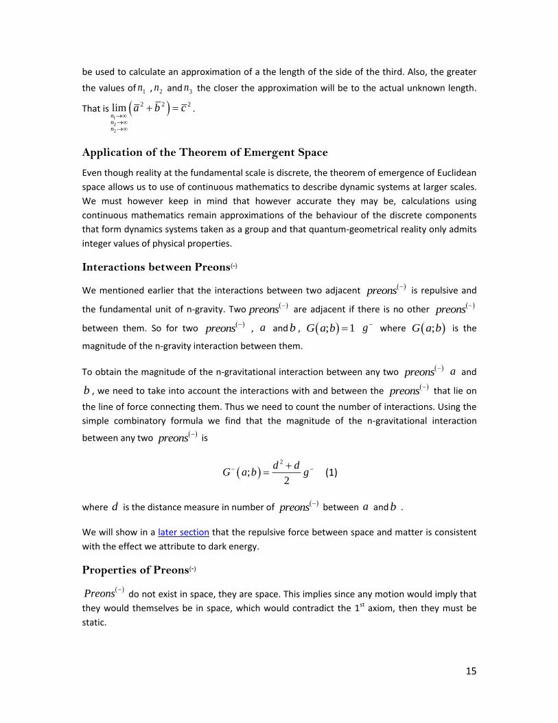
Interactions between Preons(-)
We mentioned earlier that the interactions between two adjacent preons
is repulsive and
the fundamental unit of n-gravity. Two preons
are adjacent if there is no other preons
between them. So for two preons
, a and b , ; 1G a b g
where ;G a b is the
magnitude of the n-gravity interaction between them.
To obtain the magnitude of the n-gravitational interaction between any two preons
a and
b , we need to take into account the interactions with and between the preons
that lie on
the line of force connecting them. Thus we need to count the number of interactions. Using the
simple combinatory formula we find that the magnitude of the n-gravitational interaction
between any two preons
is
2
;2
d dG a b g
(1)
where d is the distance measure in number of preons
between a and b .
We will show in a later section that the repulsive force between space and matter is consistent
with the effect we attribute to dark energy.
Properties of Preons(-)
Preons
do not exist in space, they are space. This implies since any motion would imply that
they would themselves be in space, which would contradict the 1st axiom, then they must be
static.
16
And since they are fundamental, preons
do not decay into other particles the number of
preons
is finite and constant which implies that quantum-geometrical space is finite and that
the Universe is finite.
Emerging Space and the Notion of Dimensions
We think of spatial dimensions as if they were physical in the way matter and space are physical,
but the concept of dimensions is a relational concept which allows us to describe of the motion
(even if that motion is nil) of an object or set of objects a relative to an object or set of objects
b taken as a reference. Different systems of reference having directions and speeds relative to
a given object or set of objects give different measurements of their positions, speed, mass and
momentum and, according to dominant physics theories, there is no way to describe the motion
of a reference system relative to space (or absolute motion), thus no way to know anything but
relative measurements of properties are such as mass, energy, speed, momentum or position.
However, if QGD is correct in its description of space, then each fundamental unit of space is a
distinct permanent position relative to all other discrete components of space ( preons
being
static) so that quantum-geometrical space can be taken as an absolute reference system which
allows the measurements of the absolute mass, energy, momentum and position of any physical
objects within our Universe.
Of course, assuming that space is quantum-geometrical, the question as to whether or not it is
possible to measure or even detect absolute motion must be answered and will be once we
have established the basics of QGD. For now, we will focus our attention on essential
distinctions between how we represent quantum-geometrical space from representation
continuous space.
Dimensions are geometrical constructs which allows us to map to analyse how objects relate to
each other.
The dimensionality of space is the number of elements in the largest possible set of non-
concurrent and mutually orthogonal lines that can be drawn through a preon
. Space being
an emergent property of preons
and all
preons
having identical fundamental intrinsic
properties, and all interacting to create space, then space must be isotropic. It follows that since
all preons
in the Universe interact with each other, it is possible to determine the distance
and magnitude of the interactions between any given preon
the
preons
lying on each
line of an orthogonal set.
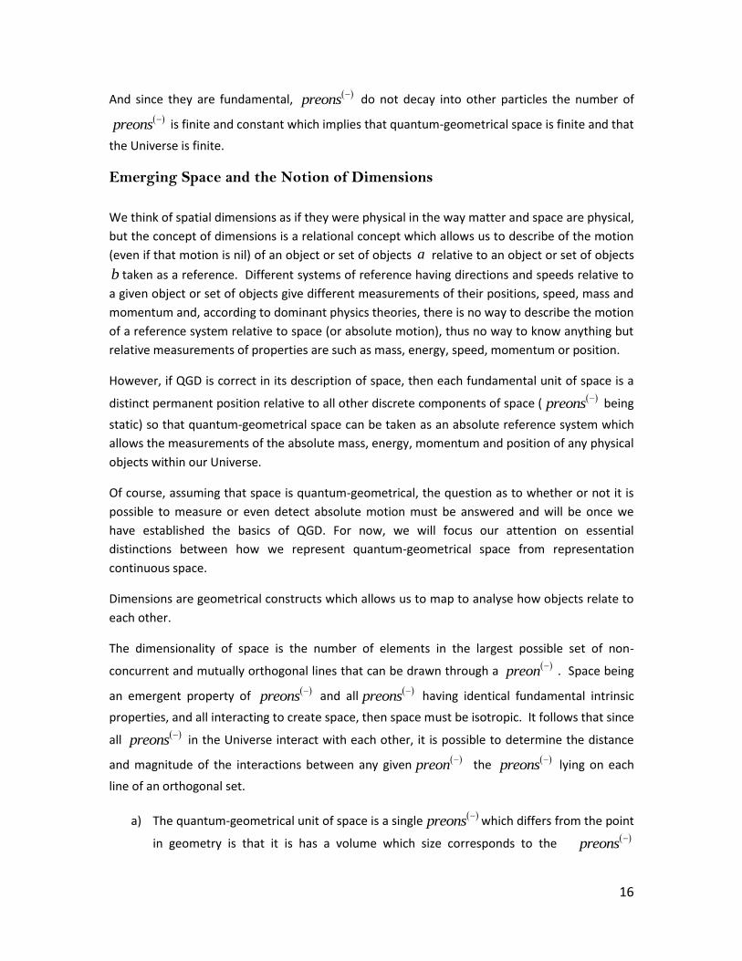
a) The quantum-geometrical unit of space is a single preons
which differs from the point
in geometry is that it is has a volume which size corresponds to the preons
17
fundamental unit of matter. So though we can make each preons
correspond to a
point in geometrical space, the point has a volume equal to one
b) The distance between two adjacent preons
is the fundamental unit of distance and
by definition cannot be divided in smaller units. So there the distance between any two points is an integer
c) A set L of preons
for which all lines force acting between them coincide maybe
understood as a segment of a line. But such a segment in not one-dimensional since it is
being made of preons
and therefore has a volume equal the number of preons
it
contains.
d) The maximum number of mutually orthogonal lines with a common preon
, the origin
is three
e) All preons
are part of the Universe, that is
pa U , where a is any given
preon
and p
U is the set of all preons
.
f) All preons
interacts gravitationally with each other so that
g) a preon
a such that a L interacts n-gravitationally with all
preon L and
the magnitude of each interactions depends on the quantum-geometrical distance
between a and each of the preons
of L and
h) if a L , the distance from it is zero and ; 0G a b
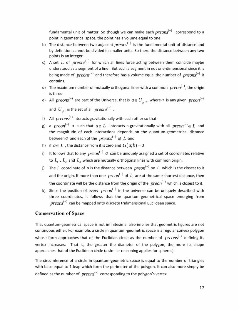
i) It follows that to any preon
a can be uniquely assigned a set of coordinates relative
to 1L , 2L and 3L which are mutually orthogonal lines with common origin,
j) The i coordinate of a is the distance between preon
on iL which is the closest to it
and the origin. If more than one preon
of iL are at the same shortest distance, then
the coordinate will be the distance from the origin of the preon
which is closest to it.
k) Since the position of every preon
in the universe can be uniquely described with
three coordinates, it follows that the quantum-geometrical space emerging from
preons
can be mapped onto discrete tridimensional Euclidean space.
Conservation of Space
That quantum-geometrical space is not infinitesimal also implies that geometric figures are not
continuous either. For example, a circle in quantum-geometric space is a regular convex polygon
whose form approaches that of the Euclidian circle as the number of preons
defining its
vertex increases. That is, the greater the diameter of the polygon, the more its shape
approaches that of the Euclidean circle (a similar reasoning applies for spheres).
The circumference of a circle in quantum-geometric space is equal to the number of triangles
with base equal to 1 leap which form the perimeter of the polygon. It can also more simply be
defined as the number of preons
corresponding to the polygon’s vertex.
18
Since both the circumference of a polygon and its diameter have integer values, the ratio of the
first over the second is a rational number. That is, if we define 𝜋 as the ratio of the
circumference of a circle over its diameter, then π is a rational function of the circumference
and diameter of a regular polygon.
This implies that in quantum-geometric space the calculation of the circumference or area of a
circle or the surface or volume of the sphere can only be approximated by the usual equations
of Euclidian geometry.
The surface of a circle would be equal to the number of preons
within the region enclosed
by a circular path.
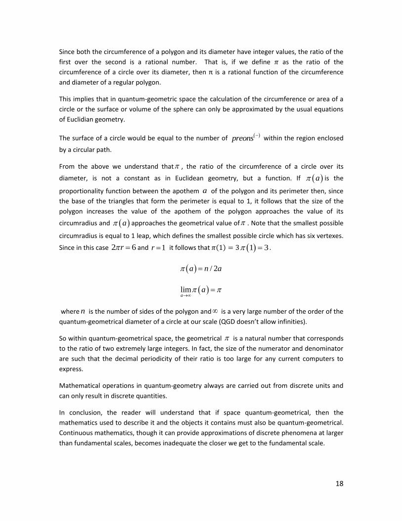
From the above we understand that , the ratio of the circumference of a circle over its
diameter, is not a constant as in Euclidean geometry, but a function. If a is the
proportionality function between the apothem a of the polygon and its perimeter then, since
the base of the triangles that form the perimeter is equal to 1, it follows that the size of the
polygon increases the value of the apothem of the polygon approaches the value of its
circumradius and a approaches the geometrical value of . Note that the smallest possible
circumradius is equal to 1 leap, which defines the smallest possible circle which has six vertexes.
Since in this case 2 6r and 1r it follows that 𝜋(1) = 3 1 3 .
/ 2a n a
lima
a
where n is the number of sides of the polygon and is a very large number of the order of the
quantum-geometrical diameter of a circle at our scale (QGD doesn’t allow infinities).
So within quantum-geometrical space, the geometrical is a natural number that corresponds
to the ratio of two extremely large integers. In fact, the size of the numerator and denominator
are such that the decimal periodicity of their ratio is too large for any current computers to
express.
Mathematical operations in quantum-geometry always are carried out from discrete units and
can only result in discrete quantities.
In conclusion, the reader will understand that if space quantum-geometrical, then the
mathematics used to describe it and the objects it contains must also be quantum-geometrical.
Continuous mathematics, though it can provide approximations of discrete phenomena at larger
than fundamental scales, becomes inadequate the closer we get to the fundamental scale.
19
The Concept of Time
The single most misleading concept in physics is that of time.
Although time is a concept that has proven useful to study and predict the behaviour of physical
systems (not to mention how, on the human level, it has become an essential concept to
organize, synchronize and regulate our activities and interactions) it remains just that; a
concept.
Time is a relational concept that allows us to compare events with periodic systems; in other
words, clocks. But time has no more effect on reality than the clocks that are used to measure it.
In fact, when you think of it, clocks don’t really measure time. Clocks count the number of
recurrences of a particular state. For instance, the number of times the pendulum of a clock will
go back to a given initial position following a series of causality linked internal states. So clocks
do not measure time, they count recurrent states or events.
If clocks do not measure time, what does?
That answer is nothing can. There has never been a measurement of time and none will ever be
possible since time is non-physical. Neither has there been or ever will be a measurement of a
physical effect of time on reality. Experiments have shown that rates of atomic clocks are
affected by speed and gravity, but these are slowing down of clocks and not a slowing of time.
Yet, as useful the concept of time may be, it is not, as generally believed, essential to modeling
reality. In fact, taking the concept of time out of our descriptions of reality solves a number of
problems.
For instance mass, momentum, speed and energy are intrinsic properties thus different
observers will measure the same mass, speed, momentum and energy regardless of the frame
of reference they use.
And if time does not exist, neither does time dilation. Time dilation and the implied assumption
of space continuum are essential to explain the constancy of the speed of light in special
relativity. But neither is necessary in QGC since the constancy of the speed of light follows
naturally from the discreteness of space.
Finally, if time does not exist, then although the unification of space (a representation of space
to be precise) and time (which is a relational concept) into mathematical space-time provides a
useful framework in which we can study the evolution of a system, physical space-time makes
no sense.

20
The Quantum-Geometrical Nature of Matter
If space is discrete, then matter, which exists in quantum-geometrical space must also be
discrete. Not only must it be discrete, but it must fit the discrete structure of quantum-
geometrical space. That is, it should correspond to the amount of matter which can occupy the
quantum of space that is the preon
. We assigned the name preon
, symbol 𝑝(+), to the
fundamental particle of matter. QGD assumes that preons
is the only fundamental particle
of matter, hence all other particles are composite particles made of preons
.
Preons
are fundamental so, to be in agreement with our definition of what constitutes a
fundamental particle, they do not decay into other particles or composed of other particles as a
consequence they are conserved throughout the entire existence of the universe. This implies
that the amount of matter of the universe remains constant and finite throughout its existence.
Also, in the same way that the interactions between two preon
is the fundamental unit of n-
gravity or g , the interactions between two
preon is the fundamental unit of p-gravity or
g . Here however, while n-gravity is a repulsive force acting between
preons
from which
emerges quantum-geometrical space, p-gravity is an attractive force acting between preons
1.
In addition to carrying the fundamental force of p-gravity, preons
are strictly kinetic particles
and as such have momentum. The properties of fundamental particles must evidently also be
fundamental, so the momentum of a preon
is fundamental, that is, it never changes. Also
fundamental is the fundamental speed of the preon
which as we will see must be deduced
from its momentum using the QGD’s definition of speed we will introduce later and shown to
be equal to the speed of light.
Preon(+)| Preon(+) pairs
If preon
are the fundamental unit of space, then they must at most hold one fundamental
unit of matter. If the preon
could hold n
preons
than then fundamental unit of space
with be
preon
n
or one thn which would be inconsistent with axiom 1. Therefore, there is the
exclusion principle by which a preon
can only host a single
preon
.
1 We will show in the section about the formation of particles how p-gravity binds
preons
into
particles and structures.
21
The preon
is strictly kinetic and moves by leaping from preon
to preon
. If it exist, it
must occupy space and so transitorily must pair with preons
along its path. And since
preons
and preons
are fundamental, that is, they and their intrinsic properties are
conserved, preon
| preon
pairs must interact with each other through both n-gravity and
p-gravity.
Propagation
Propagation implies motion; the displacement of matter ( preons
) through quantum-
geometric space. A preon
a will leap from the
preon
it is paired with to the next adjacent
preon
in direction of its momentum vectoraP .
Two preons
1p and
1p are adjacent if 1 2; 1G p p
.
The preonic leap is the fundamental unit of displacement and determines the fundamental
speed of preons
. We will show that the speed of light and its constancy are direct
consequence of the structure of quantum-geometrical space and the speed of preons
.
Interaction
Interactions through the n-gravity and p-gravity do not require the displacement or exchange of
matter. So unlike propagations, interactions are not mediated by quantum-geometric space (
preons
).
We already explained that quantum-geometric space emerges from the interactions between
preons
; the n-gravity field between them. N-gravity does not propagate through quantum-
geometric space since it generates it. It follows that n-gravity is instantaneous.
P-gravity, the force acting between preons
is similarly instantaneous and, as we will see later,
so must be the resultant effects of n-gravity and p-gravity.
22
Mass, Energy, Momentum of Particles and Structures
We will now derive the properties of mass, energy, momentum and speed from the axiom set of
QGD.
Mass
The fundamental units of matter are preons
. The mass of any particle or structure is an
intrinsic property and corresponds to the number of preons
that compose it.
We will show that this simple and natural definition of mass is the only one required to describe
any physical system.
Also, as an intrinsic property, mass is observer independent (see here for the way by which we
can obtain the intrinsic mass of an object).
Energy
The fundamental unit of energy corresponds to the kinetic energy of the preon
which is equal
to the magnitude of its momentum vector c . That is pE P c c .
Note that we use the symbol c because, as we will show that the fundamental energy of a
preon
is numerically equal its momentum and to its speed, the latter being equal to the
speed of light.
From our definitions of mass and energy, we find that the energy aE of an object a is equal
product its mass am (the number of preons
it contains) by the fundamental energy of the
preon
. That is:
1
am
a i a
i
E c m c
(2)
For a single preon
we have 1
pm so ip
E c c .
Momentum
The momentum vector of a preon
is fundamental. It never changes magnitude, but when
bound within a structure preons
their follow bounded trajectories. That is, the directions of
the component vectors change as they follow trajectories determined by the inner interactions
acting between them.
23
The momentum of a body of a is the magnitude of its momentum vector 1
am
a i
i
P c
, that is:
1
am
a a i
i
P P c
(3).
But since1 1
maxa am m
i i a
i i
c c m c
then1
0am
i a
i
c m c
; the maximum momentum of an
body is equal to its energy which occurs in structures when the trajectories of bound preons
are parallel.
Velocity
The velocity of a particle or structure follows naturally from QGD’s axiom set and corresponds to
the ratio of its momentum vector over its mass. That is:
1
am
i
ia
a
c
vm
(4) .
And since both momentum and mass are intrinsic, thus frame independent, so it must be of
velocity. We’ll call the speed as defined in equation (4) as the intrinsic speed.
Therefore, the conventional concept of velocity is not a measure of the intrinsic velocity, but
really a measure of distance; specifically the distance travelled by an object in a given direction
between periodic events (the tics of a clock for example). As for the distance travelled, we
understand that it is relative to the frame of reference against which the measurement is made.
The velocity given as the ratio the relative distance over time (which basic unit is the number of
recurrence of the state of a periodic system), we will call conventional relative speed or simply
the relative speed.
If as per QGD’s axioms space is quantum-geometrical, then space is a fixed structure which
provides an absolute frame of reference. We may define the absolute distance as the distance
as the distance between two positions in quantum-geometrical space (two preons
) . We will
explain later, how to derive the absolute distances between two positions from measurements
of relative distances.
We can define the absolute velocity av as the ratio of the absolute distance d and time t is
the counted number of recurrences of a chosen state of arbitrarily chosen periodic systems or
a
dv
t . The absolute velocity is distinct from the intrinsic velocity as they represent entirely

24
different physical properties and moreover properties of distinct objects. The intrinsic velocity is
a property of the particle independent of space (although displacement is consequence of the
intrinsic velocity). Absolute velocity is not a physical property as such but the measure of the
consequential displacement resulting from the intrinsic velocity. The relation between intrinsic
velocity (not relative velocity) and absolute velocity a av v is not one of equivalence but one of
proportionality. But though they have different physical meaning, we can use the they are
numerically equivalent which allows us to use the absolute velocity in QGD equations.
The Velocity of Light and Preons+
The intrinsic velocity of a preon
is
1 1
1
pm
i
i
p
p
cc
v cm
is fundamental. The velocity of light
is a direct consequence of the intrinsic speed of the preon
but only the absolute velocity of
photons can be measured (it is the two way measurement of the velocity of light). However, the
relation between the intrinsic and absolute velocity allows us to substitute the absolute velocity
of light in QGD equations for both the intrinsic velocity and momentum of the preon
and the
intrinsic velocity of photons and neutrinos.
The energy of an object is then the product of the absolute mass by the absolute speed.
Also, we can deduce the absolute speed of an object a by comparing the absolute distance a
d
it travels to the absolute distance dlight simultaneously travels. Using the relation
a
a
v d
dc
we find that a aa
d dv c c
d d
.
Time Distance Equivalence
As explained earlier, time is a useful concept but it is not physical and introduces a number of
problems when it comes to describing reality.
However, time can be advantageously replaced by a physical quantity. For example, we may use
instead use the absolute distance a photon simultaneously travels.
25
Physical Interpretation of the Equal Sign in Equations
a cE m c , the equation relating energy and mass appears which is derived naturally from
QGD’s axiom set appears very similar to Einstein 2E mc (which itself reduces to E mc
when the speed of light is taken as a unit). But there are essential distinctions between the two.
Einstein’s equation is understood as an expressing the equivalence between mass and energy.
That is, mass and energy are considered to be two forms of the same thing so mass can be
converted to energy and vice versa. This interpretation implies that pure energy (photons) and
pure mass can exist.
QGD’s equation expresses a proportionality relation between distinct physical properties that
cannot exist separately. All particles, including photons, are made of preons
and as we have
seen their mass is simply the amount of matter they contain, that is, the number of preons
they are composed from. And since preons
have an intrinsic kinetic energy, it follows that
the energy of a particle or structure is simply the number of preons
times their intrinsic
energy or a aE m c . The equal sign expresses the proportionality between an intrinsic property
of matter and the energy associated with it. So according to QGD, it is a grave mistake to assume
that the equal sign expresses physical equivalence.
QGD’s a aE m c provides a different interpretation of nuclear reactions but one that is more
consistent with observations. While the classical interpretation of Einstein’s equation implies
that nuclear reactions result in a certain amount of mass being transformed into energy, QGD
model suggests is that during a nuclear reaction, mass is not transformed into energy, but
rather, bound particles are freed from the structures they were bound into and carry with them
their momentum. According to QGD, there is no conversion of mass into energy, but only the
release of particles having momentum.
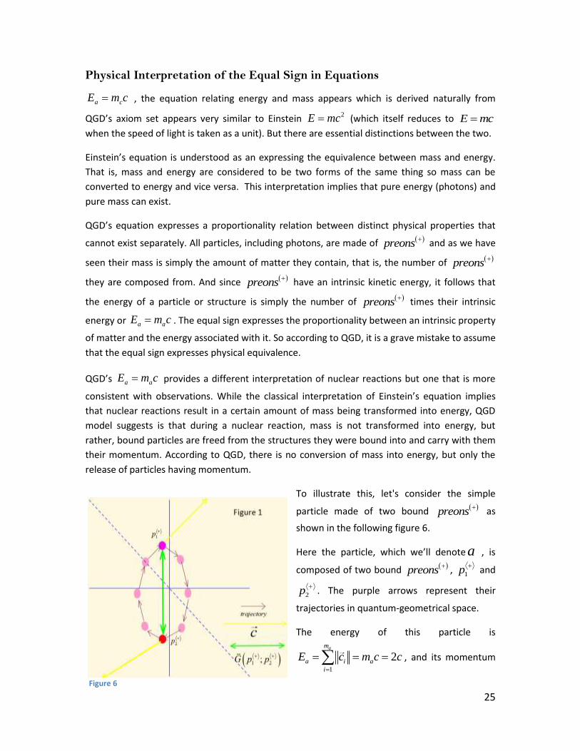
To illustrate this, let's consider the simple
particle made of two bound preons
as
shown in the following figure 6.
Here the particle, which we’ll denote a , is
composed of two bound preons
,
1p
and
2p
. The purple arrows represent their
trajectories in quantum-geometrical space.
The energy of this particle is
1
2am
a i a
i
E c m c c
, and its momentum
Figure 6
26
is1 2
1
0am
a i
i
P c c c
. This system has zero momentum, hence cannot impart
momentum to any other structure or particle.
But if as a result of a nuclear reaction the bound between the component preons
of the
particle was broken, the energy of this system would remain the same but the momentum of
the system would be equal to the sum of the momentum of the now free preons
. In this
simple case, the momentum of the system would be equal to its energy
1 2
1 2,2
p pP c c c . And the momentum that the system can impart is 2c . The
amount of mass and energy of this two preons
system does not change as a result of a
nuclear reaction. What changed is the momentum of the system which is interpreted the energy
of the system and incorrectly attributed to a conversion of mass into energy. This will be
discussed in detail in the appropriate sections of this book.
*
Another example in which it is the QGD interpretation of the equal sign is necessary is in special
cases where the component preons
of a particle or structure move on parallel trajectories.
In such case we find that that 1 1
a am m
a i i a
i i
P c c E
. That is, for such special cases there
number of units of momentum found on the left is equal to the number of units of energy we
have on the right. But though the number of units are equal, the units are units of different
properties and we must always keep in mind that the units on the left are units of momentum
while those on the right are units of energy. They may be numerically equal, but they represent
two distinct properties.
Lastly, consider the properties of energy, momentum and speed of a single preon
.
1
pm
ipi
E c c c
units of energy
1
pm
ipi
P c c c
units of momentum
1
1
am
i
i
p
p
cc
v cm
units of speed
27
Here we have three distinct intrinsic properties which are quantitatively equal but qualitatively
different. So though from the equation above we can derive p p p
E P v c we have to
remember that c is a fundamental quantity of several distinct fundamental properties.
The necessity of the distinction between mathematical and physical interpretations becomes
evident since for most particles and structures p p p
E P v .
The physical and mathematical interpretations of the relations between physical properties can
differ significantly and ignoring such differences leads to incorrect assumptions about nature.
For instance, in the section on optics, we will show that the quotient of a Euclidean division of
the momentum of a photon over the mass of a particle corresponds to the absorbed part of the
photon while the remainder of the operation is the reflected part. The physical interpretation of
the mathematical must be derived from the theory’s axioms.
The Relation between Object and Scale
A group of preons
maybe treated as a single object a in regards to a given interaction if the
effects of the interaction on the object can be fully described in terms of the object’s dynamic
properties such as its mass am , its momentum 1
am
i
i
c
or its velocity 1
am
i
ia
a
c
vm
, etc.
A physical scale maybe understood as a group objects which can be described as above under a
given interaction.

28
Forces, Interactions and Laws of Motion
The dynamics of a particle or structure is entirely described by its momentum vector. The
momentum vector can be affected by forces, which imply no exchange of particles. The
momentum vector of a particle or structure can also be affected by interactions during which
two or more particle of structures will exchange lower order particles or structures. These are
non-gravitational interactions which result in momentum transfer or momentum exchanges.
We will show how all effects in nature result from one or a combination of these two types of
interactions.
Gravitational Interactions and Momentum
According to QGD, there exist only two fundamental forces: n-gravity which is a repulsive forces
acting between preons
and p-gravity, an attractive force which acts between
preons
and
gravity as we know it is the resultant effect of n-gravity and p-gravity.
Preons
exist in quantum-geometrical space which is composed of
preons
.
Preons
are
also strictly kinetic so they must move by leaping from preons
to
preons
and, between
leaps, transitorily pair with preons
to form
|preon preon
pairs (which we will represent
by
preon ) which because of conservation of fundamental properties interact with other
|preon preon
pairs through both n-gravity and p-gravity. It follows that since all particles
or structures are made of |preon preon
pairs, they must interact through both n-gravity
and p-gravity.
The combined effect of the n-gravity and p-gravity is what we call gravity. Hence gravity,
according to QGD, is not a fundamental force but an effect of the only two fundamental forces it
predicts must exist.
;G a b , the gravitational interaction between two material structures ace a andb , is the
combined effect of the n-gravity and p-gravity interactions. So, to find ;G a b we simply need
to count the number of n-gravity and p-gravity interactions and vector sum them. We do this as
follows:
Since a and b respectively contain am and bm preons
and since every
preon
of a
interacts with each and every preon
of b , the number of p-gravity interactions is given by
the product a bm m or the product of their masses in preons
.

29
The n-gravity effect between a preon
of a and a preon
b , the force that space exerts on
a and on b , is the sum of n-gravity interactions between them. Given a quantum-geometrical
distance d , which is the number preons
from a
preon ofa and a
preon
ofb
(including a and b ) and given that all preons
between a and b interact with each other,
the number of n-gravity interactions is given by
2
, ,
2
i j i jd d
, where i and j respectively
correspond to the thi
preon of a and the
thj
preon of b . And since a andb
respectively contain am and bm
preons , then the total number of n-gravity interactions
between them is
2
, ,
11
2
j
i
m
mi j i j
ij
d d
.
Using the relation g k g we can express p-gravity in units equivalent to the magnitude of
an n-gravity interaction which allows us to find the resulting effect from n-gravity and p-gravity
interactions between a andb . Thus the gravitational interaction between a andb is given by
2
, ,
1
1
2;
j
i
m
m
i j i j
i
j
a b
d dG a b m m k
where the first component, a bm m k ,is the magnitude of the p-
gravity force acting between a andb and
2
, ,
11
2
j
i
m
mi j i j
ij
d d
is the magnitude of the n-gravity force
between them. It is interesting to note here that
2
, ,
11
2
j
i
m
mi j i j
ij
d d
is the force exerted by quantum-
geometrical space itself on two particles or structures.
At larger scales, for homogeneous spherical structures, we find that
2 2, ,
11
2 2
j
i
m
mi j i j
a b
ij
d d d dm m
where d is the distance between the centers of gravity of a and
b . This allows us to derive the simplified gravitational interaction equation
2
;2
a b a b
d dG a b m m k m m
or
2
;2
a b
d dG a b m m k
.

30
The reader should note that according to the QGD equation for gravity, the p-gravitational
interaction is independent of distance. It is the number of n-gravitational interactions between
two bodies, which is proportional to the square of the number of preons
between them (the
physical distance), that causes variations in the magnitude of the gravity. As we will now see, the
effect of gravity on momentum (and speed) results from variations in distance. It space’s
repulsive force determine the dynamics of systems.
The Fundamental Momentum and Gravity
That the momentum of the preon
is fundamental is a postulate of QGD. It is equal to
p
P c c . In fact, of all properties of the preon
, only its direction is variable. And the
only thing that affects it is gravity.
The direction of a
preon
is determined by the resultant of the gravitational interactions
acting on it, which interactions are with free
preons
, particles or structures and if the
preon
is bound, with the
preons
that is it bound to.
A change in direction of a
preon
is proportional to the change in the resultant of the forces
acting on it. That is:
1 2
2 1
p p s ss s
P P G
where 1 2 1 2 1 21 1
; ;am n
i j i ks s s s s s
j k
G G p p G p a
is the
resultant of the forces acting on the
preon
and is the directional vector sum which we
define as
1 21
2
1 21
1 21
ps s
s
sps s
s
ps s
s
P G
P G c c
P G
.
The directional vector sum describes the conservation of the momentum of the
preons
. The
result of the directional is the normalized vector sum of the momentum vector of the
preon
and the variations in gravity vector G between states 1s and 2s .
Newton’s first law of motion is implied here since for 0G we have
1
p p
s s
P P
.
We will see how Newtonian gravity emerges from gravitational interactions at the fundamental
scale.
31
Gravity between Particles and Structures
Astrophysical observations which we shall discuss later suggest that 10010k , so that at short
distances, the number of n-gravitational interactions being very low and the magnitude of the
force being over a hundred orders of magnitude weaker than p-gravity.
2
;2
a b
d dG a b m m k
The n-gravitational component of QGD equation for gravity is insignificant compared to the p-
gravitational component. Gravity at short scales being over a hundred orders of magnitude
stronger than at that at large scales, it is strong enough to bind preons
into composite
particles and composite particles into larger structures.
Bound
preons
form particles and structures which then behave as one body which dynamic
property is described by the momentum vector 1
am
a i
i
P c
which magnitude is its momentum.
That is 1
am
a a i
i
P P c
. Because of that, the dynamics of particles and structures can be
described simply as the evolution of their momentum vector aP from state to state.
Particles and structures are in constant gravitational interactions with all particles and structures
in the entire universe. The direction of the momentum vector of a particle or structure at any
position is the resultant of its intrinsic momentum and extrinsic interactions. Hence, if the
structure of a particle or structure and its interactions remain constant, so will its momentum
vector. Changes in momentum are due to variations in the magnitude and direction of the
gravitational interaction, hence due to variations in their positions.
For simplicity, we will start by describing the dynamics of a system consisting of two
gravitationally interacting bodies.
Consider bodies a and b in state 1s which interact gravitationally in accordance to the
equation 1
2
;2
a bs
d dG a b m m k
. Change in the momentum vector of the bodies from
1s to the next causally related state 2s is 1 2 1 2 2 1
; ;as s s s s s
P G G a b G a b so that
11
;a a ass s
P P G a b
and 1 2 1 2 2 1
; ;bs s s s s s
P G G a b G a b so that
11
;b b bss s
P P G a b
where 2s is a successive state of our two body system.
32
Here xx
c v
c
preserves the fundamental limit of the momentum of a particle or structure
which we have shown cannot exceed its energy; that is: 1 1
x xm m
i i
i i
c c
. The bracket is the
ceiling function so that for xc v we have 1xc v
c
and 1 2 1 2
;xs s s s
P G a b but for
xv c we have 0xc v
c
and1 2
0xs s
P . And since the momentum of a particle or
structure cannot exceed its energy, its maximum speed is 1max
xm
i
xix
x x
cm c
v cm m
.
Note that for descriptions of dynamics system at speed below the speed of light, will simply
write 11
;a ass s
P P G a b
and 11
;b bss s
P P G a b
with the understanding that x is implicit
and equal to 1.
Note: It is important remember that QGD gravity is the resulting effect of two
distinct forces, p-gravity (attractive) and n-gravity (repulsive). The p-gravity being a
function of mass only and n-gravity being a function of mass and distance, the p-
gravity and n-gravity components of the equation must always be differentiated
separately then added to calculate variations in gravity.

33
Derivation of the Weak Equivalence Principle
The weak equivalence principle or universality of free fall is easily derived from QGD’s equation
for gravity 2
;2
a b
d dG a b m m k
where am and bm are respectively the masses of a
and b and d the distance, all in natural fundamental units.
According to QGD, the change in momentum due to gravity following the change in positions
between two successive states 1s and 2s is equal to the gravity differential between the two
positions ;G a b . That is: 1 2 1 2
;as s s s
P G a b .
QGD defines speed of a body as a
a
a
Pv
m and the acceleration of a body is
a
a
a
Pv
m
.
Since ;bP G a b , the acceleration of an object a due to the gravitational interacting
between a and b is ;a
a
a a
P G a bv
m m
Since
2 2 2 2
1 1 2 2 1 1 2 2;2 2 2 2
a b a b a b
d d d d d d d dG a b m m k m m k m m k k
then
2 2 2 2
1 1 2 2 1 1 2 21
2 2 2 2b a b b
a
d d d d d d d dv m m k k m k k
m
.
Therefore, gravitational acceleration of a body a relative a second body b is independent of
the mass of the first and dependent on the mass of the second. Conversely, the gravitational
acceleration of an object b relative to a is given by
2 2
1 1 2 2
2 2b a
d d d dv m k k
is independent of bm . So, regardless of their mass
am , all bodies a will be accelerated relative to a given body b at the same rate.
We have shown that the weak equivalence principle is a direct consequence of QGD’s equation
for gravity which itself is derived from QGD’s axiom set.

34
However, it is essential to keep in mind that the acceleration of a first body relative to a second
body is independent of the mass of the first body does not mean that the effect of gravity on an
object, the change in momentum it produces, is independent of its mass.
But unlike gravitational acceleration, the resultant change in momentum is dependent on the
mass of the accelerated body. A body a that is n times as massive as a body a will experience
a change in momentum n times greater. The measurement of acceleration alone does not
provide a measurement of the effect gravity has on distinct bodies.
A major problem with classical mechanics description of gravity is how it relates force to
acceleration and considers the change in momentum to be a consequence of the effect of a
force on speed and not, as it should, the reverse. Classical momentum is also defined as the
product of the speed of a body and its mass. Speed is function of time, which is a pure relational
concept, and mass is a conventional definition and not a fundamental property of matter.
Note: The equation 2 2
1 1 2 2;2 2
a b a b
d d d dG a b m m k m m k
may not be
algebraically simplified to 2 2
1 1 2 2;2 2
a b
d d d dG a b m m
since the information
as to whether id d , id d or id d would be lost and there would be no way to know
whether the gravitational interaction at 1d or 2d is attractive or repulsive (or one of each), thus
no way to know if a body b is gravitationally accelerated or decelerated relative to a . For
instance, if 2 1d d , b would accelerate away from a when 1d d and 2d d but would
accelerate towards a when 1d d and 2d d .
Therefore, the gravitational interaction at each the initial and following positions must be
calculated first, which gives the proper sign to each (negative meaning repulsive and positive
meaning attractive) and only then should ;G a b be calculated. Finally, ;G a b has a
different physical interpretation depending on whether id d , id d or id d .
So a body b moving away from a body a will be decelerated by the gravitational interaction
between them until it reaches a distance d and will be accelerated from that distance on. It
follows that a particle that moves at a less than the speed of light will be accelerated if the
distance it travels is greater than d (approximatively 10MPS). The greater the distance from
the source beyond d , the greater its speed will be when it reaches the Earth. Particles moving
at the speed of light are unaffected (see Why Nothing Moves Faster than the Speed of Light).
The repulsive gravitational effect predicted by QGD between structures over large distances is
supported by the recent discovery known as the dipole repeller.
35
According to QGD, the momentum vector of object is an intrinsic property given by 1
am
i
i
c
where the mass, am , is the number of bounded
preons
of a and each ic correspond to the
momentum vector of a bound
preon
. The speed of object is given by 1
am
i
i
a
c
m
.
Gravity affects the resultant trajectories of the component preons
, which changes the
momentum. The change in speed is a consequence of the change in momentum and not the
reverse.
Given two object a and b both at the same distance from a massive structure, it is impossible
to distinguish between them based on their respective acceleration, which makes acceleration
the wrong property to measure if one wants to compare the effect of gravity on particles or
structures.
Variations in the gravitational interaction affect directly and instantaneously the momentum of
the interacting bodies. It is the variations in momentum that determine the variations in speed
and not the reverse.
Comparison between the Newtonian and QGD Gravitational Accelerations
From 2 2
1 1 2 2
2 2b a
d d d dv m k k
we have
2 2
1 1 2 2 ;2 2
b b a b
d d d dm v m m k k G a b
which is equivalent to Newton’s
second law of motion relating force, mass and acceleration aF m v where ;F G a b .
The equations are very similar and it would be tempting to equate Newton’s second law and its
QGD equation, but this cannot be done directly.
Newtonian gravity varies with distance and is time independent. However Newton’s second law
of motion when applied to gravity ignores the distance dependency but threats the force as if it
were constant. And most importantly, despite the fact that Newtonian gravity is instantaneous
(as must be its effects) Newtonian mechanics introduces a time dependency on the effect of
gravitational acceleration. The introduction of the time dependency of the gravitational
acceleration is not in agreement with Newton’s law of gravity. And while the time dependency
approximates its dependency on distance (since d t and b bv v where bv is the
classically defined speed) it introduces delays on the action which according to Newton’s law of
gravity does not exist.

36
Newton’s second law of motion applied to gravity gives ;
b
b
G a b tv
m
where ;G a b
represents the Newtonian force of gravity. Since the QGD equation is ;
b
b
G a bv
m
, it
follows that ; ;G a b t G a b . But the assumed time dependency of the effect introduces
a delay in the effect of gravity on the momentum of a body while it should be instantaneous. So
for Newtonian mechanics we have ;
b
b
G a bv
t m
while in QGD
;b
b
b b
G a bPv
m m
. So
the Newton’s law of motion introduces a delay of ;
b bm vt
G a b
.
Such delays of the effect of gravitational acceleration are very small since the distance between
two positions in quantum-geometrical space is fundamental, and it would be difficult if not
impossible to detect over short variations in distance, especially if there are no changes in
direction of the gravitationally accelerated body. But over an astronomical number of changes in
direction, such as experienced by a planet orbiting the sun, the predicted delays would add up
to observable differences with the observed motion of the planet. As we will discuss in detail
later in this book by removing the time dependency in accordance to QGD, Newtonian gravity
can predict the precession of the perihelion of Mercury.
If correct, the discrepancy between Newtonian mechanics’ prediction of the motion of Mercury
and observation is due to the time dependency introduced when using Newton’s second law of
motion; incorrectly making the effect of an instantaneous force dependent on time.
It is also interesting to note that the application of general relativity to the motion of Mercury
(or other bodies) does the exact opposite since the effect of a change in position of a body in a
gravitational field instantly changes its direction because it instantly follows the predicted
geodesics. This may explain why general relativity correctly predicts the precession of the
perihelion of Mercury.
Non-Gravitational Interactions and Momentum
The momentum of a particle or structure may also change as the result of absorption of
particles.
For example, if a absorbs a photon then 2 1
a as s
P P P . Similarly, if it emits a photon then
2 1
a as s
P P P . Note that depending of the relative direction of a and the absorbed photon, 2
as
P
may be greater or smaller than 1
as
P .

37
The mass of particle or structure increases or is reduced by an amount that is equal to the mass
of the absorbed or emitted photon (or other particle).
Since 1
2
2
as
as a
s
P P
vm
and 2
2
as
as
Pv
m
the acceleration is inversely proportional to the mass of the
object that is accelerated. Gravitational acceleration being independent of its mass, there is no
equivalence between gravity and non-gravitational acceleration as suggested by Einstein’s
famous thought experiment. We will show that it is possible to distinguish the effect of gravity
from constant acceleration because their effect on mass, momentum and energy are different
for different bodies.
38
Application to Celestial Mechanics
If gravity is instantaneous, then its effects are also instantaneous. It follow that a body is always
at equilibrium with the gravitational forces acting on it. We will call this the principle of
equilibrium.
As we will see, the principle of equilibrium governs all dynamics of all gravitationally interacting
system, thus will be central to QGD’s description of the motion of gravitationally interacting
celestial objects.
Therefore, the change in momentum of a body from one position to the next corresponds to the
change in the instantaneous change in net magnitude of the forces acting on it between the two
positions. We will now see how this applies to describe the motion of a planet orbiting a star.
From the principle of equilibrium it follows that at a position ip the momentum of a body b
gravitationally interacting with a body a is given by 1
1
;i i
i i
b bp p
p p
P P G a b
where 1ip is the
preceding position of b and
1
1 1
; ; cos
; ;
;
i i
i i i
i
p p
p p p
p
G a b G a b
G a b G a b
G a b
with

39
being the angle between 1
;ip
G a b
and ;ip
G a b . Orbiting bodies are a special case of which for
with 1
sin ;i i
i
bp p
p
P G a b
where is the angle between bP and the tangent of the orbit
at ip .
For any position ip , the following position is found along the direction of bP and the distance
between ip and 1ip is b
ref
vd d
c ,
refd is a reference distance chosen so that 1d
(smaller refd gives more accurate the description).
From the above equations we can deduce that the shape of the orbit of body b around a fixed
body a would be nearly circular since 1 1
; ;x x y yp p p p
G a b G a b , but bodies are in space
are in motion so since 1
;i ip p
G a b is greater when the bodies move towards each other than
when moving in opposite direction that the shape of the orbit around a moving body will be
elliptical.

40
Also, since bb
b
Pv
m then
b bb
ref ref ref
b b
P Pvd d d d
c m c E which gives an interesting relation
between the momentum and energy of b and the distance travelled. So for preons
, photons
and neutrinos, since b bP E , refd d .
N-Body Gravitationally Interactions
For a system consisting of n gravitationally interacting bodies,
11
1
;i s ss
n
a i j
j
P a aG
where ia and ja are gravitationally interacting astrophysical bodies of the system, j i and
| 1 | 1 1 | 1 1| 1 1 | 1 | 1
1
; ; ... ;n
i s j s s i s s s i s n s
j
a a G a a G a aG
where
1 | 1 | 1 | 1 | 1 | |; ; ;s i s j s i s j s i s j sG a a G a a G a a and s and 1s are successive states of the
system (a state being understood as the momentum vectors of the bodies of a system at given
co-existing positions of the bodies) and |i s xa
is the body ia and its position when at the state
s x . The position itself is denoted |ia s x
.
In order to plot the evolution in space of such a system, we must choose one of the bodies as a
reference so that the motions of the others will be calculated relative to it. A reference distance
travelled by our reference body is chosen, refd , which can be as small as the fundamental unit
of distance (the leap between two preons
or preonic leap) but minimally small enough as to
accurately follow the changes in the momentum vectors resulting from changes in position and
gravitational interactions between the bodies.
So given an initial state s , the state 1s corresponds to the state described by the positions
and momentum vectors of the bodies of the system after the reference body travels a distance
of refd . For simplicity, we will assign 1a to the reference body.
1| 1 1| 1
| 1 |
1| | 1 | 11
| | 1 | 11
; |
1 ... | ...
; |
s s
n s n s n
n
a a s j s a sj
n
a a n s j s a sj
P P G a a
s
P P G a a
(5)
41
Using the state matrix, the evolution of a system from one state to the next is obtained by
simultaneously calculating the change in the momentum vectors from the variation in the
gravitational interaction between bodies resulting from their change in position. Changes in the
momentum vectors have are as explained earlier. Changes in position are given by
1
| 1 |i
i i i
i
a ref
a s a s a
a a
v dP
v P . The distance travelled by ia from s to 1s is
1
ia
ref
a
vd
v (for 1j ,
the distance becomes simply refd ) and distance between two bodies of the system at state
s x is ; | | |i j i ja a s x a s x a s xd . It is interesting to note here that that for i j , then
; | 0i ja a s xd , so that
1 | 1 | 1 | 1 | 1 | |
2 2; | 1 ; | 1 ; | ; |
; ; ;
2 2
0
i i i j i i i i
s i s j s i s i s i s i s
a a s a a s a a s a a s
a a a a
a a a a
G a a G a a G a a
d d d dm m k m m k
m m k m m k
,
the variation in the gravitational interaction between a body with itself is equal to zero, which
implies that its momentum vector will remain unchanged unless 1n and | | 11
; 0n
n s j sjG a a
. This is the QGD explanation of the first law of motion.
42
Transfer and Conservation of Momentum
Also, a consequence of the discreteness of space is that the momentum of an object a can only
change by a multiple of its mass (each component preon
must overcome the effect of n-
gravity which are discrete units). All changes in momentum obeys must obey the law
a aP xm .
Changes in momentum due to variation in gravity are proportional to the mass of the body
subjected to it so that ; aG a b xm a aP xm law since.
Gravity and variation in gravity between two objects are multiples of their masses of the object,
but this is not the case for non-gravitational interactions.
For instance, the momentum of a photon will only in special cases be a multiple of the mass of
the object it interacts with.
For instance, for an electron e
and a photon . Then we have the three possibilities:
1. e
P xm or
2. e
P xm or
3. e
P xm where x N
In case 1, the momentum of the photon is below the minimum allowed change in
momentum of the electron. The photon cannot be absorbed (become bounded) and so will
be reflected or refracted depending on its trajectory relative to the electron.
In case 2, the photon will be absorbed and e
P xm . It this case, all its preons
will become part of the electron’s structure, the electron’s mass will increase by m its
momentum by P .
In case 3, though the photon’s momentum is greater than the minimum allowed change in
momentum for a , absorption n is not possible as it would imply a fractional change in the
momentum of eand thus is forbidden (a fractional change in momentum would imply that
material structure could move between preons
which is not possible since there is no
space which can hold them).

43
The electron can absorb the higher momentum (or energy since for photons P E ) but
to respect the a aP xm law it must simultaneously emit a photon that will carry the
excess momentum.
The emitted photon is such that e
e
PP P m
m
.
This, we shall see later, describes why atomic electrons can only absorb photons have
specific momentum and thus explain the emission and adsorption lines of elements.
Momentum Conservation and Impact Dynamics
A postulate of quantum-geometry dynamics is that space is fundamentally discrete (quantum-
geometrical, in QGD terms). If as QGD suggests the discreteness of space exists at a scale that is
orders of magnitude smaller than the Planck scale then the fundamental structure of space (and
matter) lies way beyond the limits of the observable.
That said, the discreteness of space and matter, as described by QGD, carries unique
consequences at observable scales. In fact, the laws that govern the dynamics of large systems
can be derived from the laws governing space and matter at its most fundamental.
We will now re-examine observations which, when interpreted by QGD, supports its prediction
of the quantum-geometrical structure of space, more specifically, we will show the law of
conservation of momentum at the fundamental scale explain the conservation of momentum at
larger scales.
The Physics of Collision and Conservation of Momentum
Three laws govern the physics of collision:
1. So, two objects cannot occupy the same space at the same time (a consequence of the preonic exclusion principle).
2. The momentum of particles is conserved in non-gravitational interactions.
3. Changes in the momentum of an object is a multiple of its mass or a aP xm .
For simplicity, let a and b be two rigid spheres of same volume with momentumaP and
bP ,
which are set on a direct collision course as in the figure below.
When the spheres reach the position of impact, the first law applies. Neither sphere can occupy
that position. So the spheres cannot move beyond the point of impact or, to be precise, the
intersection of the volumes of the spheres along the line of impact, which is the line that passes
through the centers of the spheres at impact.

44
To satisfy the second law, the spheres a and b in the simple example below must each emit
photons whose momentums will be exactly those of a and b respectively. That is:
1
a
i
n
a
i
m c P
and 1
b
i
n
b
j
m c P
where an and bn are respectively the numbers of photons
emitted at impact by a and b .
The photons emitted by a will be absorbed by b , imparting it their momentum and the
photons emitted by b will impart their momentum to a so that after impact 1
b
i
n
a b
i
P m c P
and1
a
i
n
b a
i
P m c P
whereaPand
bP are respectively the momentums of a and b after
impact. As a result of the impact, the spheres will move in opposite direction at speed
b
a
a
Pv
m and
a
b
b
Pv
m .2
Case 2
Consider two spheres of equal mass moving in the same direction as in the figure below.
Here, at the point of impact, the forbidden component of the momentum of a in direction of b
is given by a b av v m , but the component momentum of b in direction of a is equal to zero.
2 Note that for simplicity, we ignored here the changes in the masses of the spheres due to emission and
absorption of photons. These variations in mass will be taken into account when significant.

45
That is 1
a
i
n
a b a
i
m c v v m
and 1
0b
j
n
j
m c
, hence after impact the momentums of a and
b will be
a a a b a
a
a b a
a
a b
P P v v m
PP v m
m
m v
We can see that Newton’s third law of motion is a direct consequence of the three laws
governing collision physics but that it is not due, as Newton’s third law implies, to the second
body exerting a force equal magnitude and opposite direction, but to the loss of momentum of
the first through the mechanism we have describe and which is equal to the momentum is
imparts to the second body. Newton’s third law of motion is special case of the laws of
conservation of momentum of QGD.
Consider the same setup as above. The third law says that b bP xm . Now, if a bP xm , the
momentum of a , which is the maximum momentum that it can impart, is smaller than the
minimum allowable change in momentum of b . Hence b must emit back photons in opposite
direction whose momentum is equal to the momentum of the photons emitted by a . Hence
the Newton’s third law of motion.
Case 3
So far we have discussed the special cases of the physics of collision for spheres of similar
volume which trajectories coincide. The same laws apply for all cases and when we take into
account different angles and directions we find that:
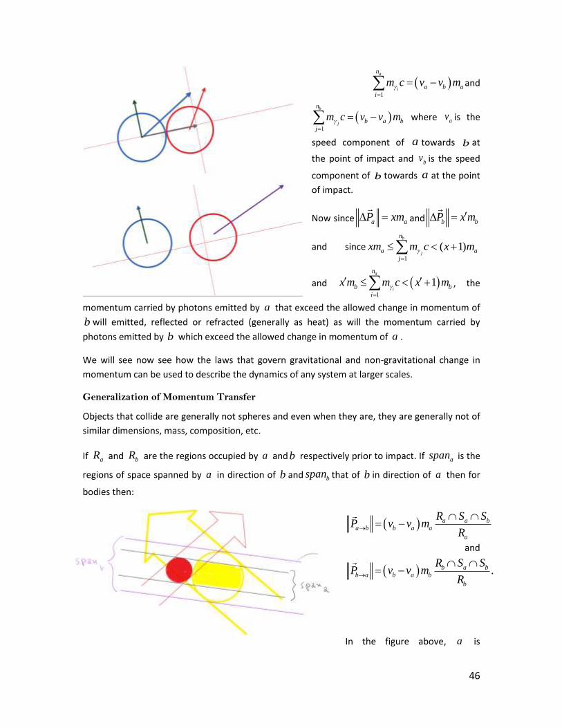
46
1
a
i
n
a b a
i
m c v v m
and
1
b
j
n
b a b
j
m c v v m
where av is the
speed component of a towards b at
the point of impact and bv is the speed
component of b towards a at the point
of impact.
Now since a aP xm and b bP x m
and since1
( 1)b
j
n
a a
j
xm m c x m
and 1
1a
i
n
b b
i
x m m c x m
, the
momentum carried by photons emitted by a that exceed the allowed change in momentum of
b will emitted, reflected or refracted (generally as heat) as will the momentum carried by
photons emitted by b which exceed the allowed change in momentum of a .
We will see now see how the laws that govern gravitational and non-gravitational change in
momentum can be used to describe the dynamics of any system at larger scales.
Generalization of Momentum Transfer
Objects that collide are generally not spheres and even when they are, they are generally not of
similar dimensions, mass, composition, etc.
If aR and bR are the regions occupied by a andb respectively prior to impact. If aspan is the
regions of space spanned by a in direction of b and bspan that of b in direction of a then for
bodies then:
a a ba b b a a
a
R S SP v v m
R
and
.b a bb a b a b
b
R S SP v v m
R
In the figure above, a is

47
represented by the sphere on the left and a a bR S S is shown in red. Similarly, b a bR S S
is in yellow. In this special illustrated here, a a a bR R S S so that a b b a aP v v m .
Note that non-gravitational acceleration is always a result of momentum transfer as described in
this section. The same principles apply whether momentum is transferred from one solid object
or from a group of particles such as in a gas. It follows that non-gravitational forces are not
forces but the effects of momentum transfer and the so-called force is simply the momentum
transferred.
The Electromagnetic Effect
Following QGD’s axiom set, in its initial state the universe only existed free preons
uniformly
distributed in quantum-geometrical space, itself dimensionalized by the interactions between
preons
.
Preons
eventually combined to form particles and particles combined to form progressively
more massive structures. The first particles to be formed were neutrinos, constituting the
cosmic neutrino background and later formed the photons that form the cosmic microwave
background radiation3. The isotropy of preons
in the initial state of the universe explains the
isotropy of the CMBR (we will show in the Cosmology section that such a universe gives rise to
the observable universe without all the problems associated with the big bang theory).
However, observations suggest that most preons
in the universe are still free or form
particles which have too small a momentum to be observed (that is: a eP m ). These
constitute what we may call the preonic background or preonic field. Magnetic fields are
created when regions of the preonic field are polarized through the interactions between the
free preons
, low momentum photons and neutrinos with charged particles.
The magnetic momentum is then understood as the momentum of the polarized region in a
given direction.
The momentum imparted by polarized preons
will cause magnetic repulsion or attraction
depending on the direction of polarization. The electro-magnetic effects will be discussed in
detail in a later section.
3 The mechanism of formation of particles and structures will be discussed in detail a section dedicated to
the topic.

48
Axiomatic Derivations of Special and General Relativity
Though the axiom sets of QGD and those of the special and the general relativity are mutually
exclusive, our theory is not exempt from having to explain observations and experiments;
particularly those which confirm the predictions of the relativity theories.
We will now derive some of the key predictions of special relativity and general relativity and
since a new theory must do more than explain what is satisfactorily explain current theories, we
will also derive new predictions that will allow experiments to distinguish QGD from the
relativity theories.
Constancy of the Speed of Light
Light is composed photons, themselves composites of preons
which move in parallel
directions.
The speed of a photon is thus
1 1
m m
i ii i
c cm c
v cm m m
which is the fundamental speed of
preons
and by
definition constant.
Why nothing can move faster than the speed of light
We know that 1
am
i
i
a
a
c
vm
and that
1 1
a am m
i i
i i
c c
then since 1 1
a am m
i ii i
a a
c c
m m
and
1
am
i
i a
a a
cm c
cm m
it follows that av c .
The Relation between Speed and the Rates of Clocks
QGD considers time to be a purely a relational concept. In other words, it proposes that time is
not an aspect of physical reality. But if time does not exist, how then does QGD explain the
different experimental results that support time dilation; the phenomenon predicted by special
relativity and general relativity by which time for an object slows down as its speed increases or
is submitted to increased gravitation interactions?
To explain the time dilation experiments we must remember that clocks do not measure time;
they count the recurrences of a particular state of a periodic system. The most generic definition
possible of a clock is a system which periodically resumes an identifiable state coupled to a
counting mechanism that counts the recurrences of that state.
49
Clocks are physical devices and thus, according to QGD, are made of molecules, which are made
of atoms which are composed of particles; all of which are ultimately made of bounded
preons
.
From the axiom of QGD, we find that the magnitude of the momentum vector of a preon
is
fundamental and invariable. The momentum vector is denoted by c the momentum is c c .
We have shown that the momentum vector of a structure is given by 1
am
a i
i
P c
and its speed
by 1
am
i
i
a
a
c
vm
. From these equations, it follows that the maximum possible speed of an
object a corresponds to the state at which all of its component preons
move in the same
direction. In such case we have 1 1
a am m
i i a
i i
c c m c
and aa
a
m cv c
m . Note here that
1
am
i
i
c
corresponds to the energy of a so the maximum speed of an object can also be defined
as the state at which its momentum is equal to its energy.
From the above we see that the speed of an object must be between 0 and c while all its
component preons
move at the fundamental speed of c .
Now whatever speed a clock may travel, the speed of its preons
components is always equal
to c . And since a clock’s inner mechanisms which produce changes in states depends
fundamentally on the interactions and motion of its component preons
, the rate at which
any mechanism causing a given periodic state must be limited by the clock’s slowest inner
motion; the transversal speed of its component preons
.
Simple vector calculus shows that the transversal speed of bound preons
is given by
2 2
ac v where av is the speed at which a clock a travels. It follows that the number of
recurrences of a state, denoted t for ticks of a clock, produced over a given reference distance
refd is proportional to the transversal speed of component preons
, that is
2 2
a
ref
tc v
d
. As the speed at which a clock travels is increased, the rate at which it
produces ticks slows down and becomes 0 when its speed reaches c .

50
We have thus explained the observed slowing down of periodic systems without using the
concepts of time or time dilation.
The predictions of special relativity in regards to the slowing down of clocks (or any physical
system whether periodic or not, or biological in the case of the twin paradox) are in agreement
with QGD however, the QGD explanation is based on fundamental physical aspects of reality.
Also, since according to QGD, mass, momentum, energy and speed are intrinsic properties of
matter, their values are independent of any frame of reference, avoiding the paradoxes,
contradictions and complications associated with frames of reference.
However, though both QGD and special relativity predict the speed dependency of the rates of
clocks, there are important differences in their explanation of the phenomenon and the
quantitative changes in rate. While for special relativity the effect is caused by a slowing down
of time, QGD explains that it is a slowing down of the mechanisms clocks themselves.
If t and t are the number of ticks counted by two identical clocks counted travelling
respectively at speeds av and av over the same distance refd then QGD predicts that
'2
2 '2 2
2 2 2
2
1
1
a
a
a a
v
c v ct t t
c v v
c
.
The speeds in the above equation are absolute so cannot be directly compared to special
relativity’s equation for time dilation which is dependent on the speed of the one clock relative
to that of the other. However, the special relativity equation can be derived by substituting for
av the speed of the second clock relative to the first clock v , then av must be the speed of
the second clock relative to itself, that is 0av , substituting in the equation above we get
2
21
tt
v
c
which the special relativity equation describing time dilation.
Then using the derivations 2 1
2 2
2 21 1
x xv tx v t
v v
c c
, y y and z z , we can easily
derive the relation between two inertial frames of reference.
51
The Relation between Gravity and the Rates of Clocks
We know that a
a
a
Pv
m then
2 2 2
2
a
ref
a
a
tc v c
d
P
m
. We have also shown that
gravity affects the orientation of the component preons
of structure so that
;aP G a b and ;
a
a
G a bv
m
and since
;a a
a
G a bv v
m
in order to predict the
effect of gravity on the rates of clocks, all we need to do is substitute the appropriate value in
2 '2
2 2
a
a
c vt t
c v
and we get
2
2
2
2
2 2 2
2
;
;1
1
a
aa
a
a a
G a bvG a b mc v
m ct t t
c v v
c
And if ; 0G a b then the equation is reduced to t t .
As we can see, the greater the gravitational interaction between a clock and a body, the slower
will be its rate of recurrence of a given periodic state. This prediction is also in agreement with
general relativity’s prediction of the slowing down of clocks by gravity.
Predictions
QGD is in agreement with special relativity and general relativity’s predictions of the slowing
down of clocks but it differs in its understanding of time. Time for the QGD being a relational
concept is necessary to relate the states of dynamical systems to the states of reference
dynamical systems that are clocks. Clocks are shown not to be measuring devices but counting
devices which mark the recurrences of a particular state of a periodic system chosen are
reference. So if clocks are understood to measure time, then time is simply the number of times
a given change in state occurs over a distance. It is not physical quantity.
We have shown that the slowing down of clocks resulting from increases in speed or the effect
gravity is explained not as a slowing down of time, but as a slowing down of their intrinsic
mechanisms.
The effects of time dilation predicted by special relativity and general relativity are both
described by
2
2
2 2
;a
a
a
G a bc v
mt t
c v
since this equation takes into account both the

52
effect of the speed and gravity on a clock. Thus, if QGD is correct, the predictions of SR and GR
are approximations of particular solutions of the QGD equation.
Although both general relativity and QGD’s predict changes in the speed of clocks subjected to
variations in the magnitude of the gravity effect, their predictions quantitatively differ. There is
hope that, in the next few years, experiments such as Atacama Large Millimeter/submillimeter
Array in Chile will discover pulsars moving in proximity to the supermassive black hole predicted
to exist at the center of our galaxy (SGR A). The predictions of general relativity would then be
tested against variations of the rate at which pulsars emit pulses as they are subjected to the
intense gravity of the black hole. QGD makes distinct predictions which could also be tested
against the same measurements.
Bending of light
The reader will recall that using the second law of motion for gravitational acceleration
introduces time delays on the effect of gravity. Since Newtonian gravity is instantaneous it is
incompatible with time dependency and, as we will see now, is the cause of the discrepancies
between the Newtonian predictions and observations.
According to QGD, photons are
composed of preons
. It follows that
photons interact gravitationally as do
all other material structure.Applying
the laws of motion to describe the
effect of gravity on the trajectory of a
photon coming into proximity to the
sun we find that a photon
changes direction at a position ip by
an angle i given by
1
; cos
2
i ii
p p
i
G
c
where i
is the angle between the vector
1
;i ip p
G S and the perpendicular
to the vector P (see figure on left).
The total angle of deflection of a photon is then
1
; cos
2
i i
i ip p
i
G
c
. The
acceleration towards the sun expressed as units of distance per units of time. At the speed c
this corresponds to a displacement of the vector 1
;i ip p
G equal to the distance travelled
+
+

53
by a photon in one second or c
units of distance (figure on the
next page). Since
1
; cos
2
i ii
p p
i
G
c
for
non-delayed gravity and
; cos
2 *2it
G
c
for
delayed gravity then 2
iit
and
; cos
22
i
ip N
ti
G
c
.
QGD and non-delayed Newtonian
gravity (which is a special case of
QGD gravity) predicted angle of
deflection is exactly twice the angle t predicted by Newtonian mechanics, hence in
agreement with general relativity and observations. That is for .875"t we get 1.75" .
So Newtonian gravity, if correctly applied, gives the correct prediction.
As a side note, it is interesting that there has never been an explanation as to why the angle of
deflection predicted by Newtonian mechanics is exactly half that of the observed deflection. Not
one third, one quarter, seven sixteenth, but exactly half.
Precession of the Perihelion of Mercury
The time dependency introduced when Newton’s second law of motion also causes errors in
Newtonian mechanics predictions of the motion of planets which causes the discrepancy
between the predicted position of the perihelion of Mercury and its observed precession. The
general equation for the angle of deviation due to gravity is
1
; cos
2
i i
i ip p
i b
G a b
P
so
the angle of non-delayed gravitational deflection of Mercury from its momentum vector at a
given position is
1
; cos
2
i i
i ip p
i b
G b
P
. The angle for delayed gravity corresponds is
UNDELAYED GRAVITY DEFLECTION DELAYED GRAVITY DEFLECTION
θ
=
=
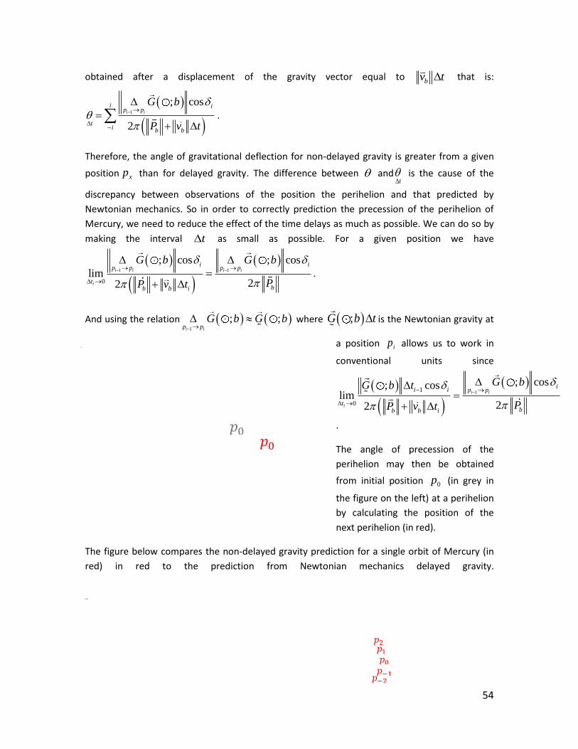
54
obtained after a displacement of the gravity vector equal to bv t that is:
1
; cos
2
i i
i ip p
ti
b b
G b
P v t
.
Therefore, the angle of gravitational deflection for non-delayed gravity is greater from a given
position xp than for delayed gravity. The difference between andt
is the cause of the
discrepancy between observations of the position the perihelion and that predicted by
Newtonian mechanics. So in order to correctly prediction the precession of the perihelion of
Mercury, we need to reduce the effect of the time delays as much as possible. We can do so by
making the interval t as small as possible. For a given position we have
1 1
0
; cos ; cos
lim22
i i i i
i
i ip p p p
tbb b i
G b G b
PP v t
.
And using the relation 1
; ;i ip p
G b G b where ;G b t is the Newtonian gravity at
a position ip allows us to work in
conventional units since
11
0
; cos; coslim
22
i i
i
ii i p p
tbb b i
G bG b t
PP v t
.
The angle of precession of the
perihelion may then be obtained
from initial position 0p (in grey in
the figure on the left) at a perihelion
by calculating the position of the
next perihelion (in red).
The figure below compares the non-delayed gravity prediction for a single orbit of Mercury (in
red) in red to the prediction from Newtonian mechanics delayed gravity.
𝑝 𝑝
𝑝
𝑝
𝑝
𝑝 𝑝

55
Orbital Decay of Binary Systems
The mechanisms using which we described and explained the precession of the perihelion of
Mercury in the preceding section also predicts the precession of binary systems. Therefore we
will not repeat the explanation here. Suffice to say all systems of gravitationally interacting
systems are governed by the same laws and described by the same equations. QGD thus
explains that the observed orbital decay such as that of the Hulse-Taylor system is not due to
loss of energy emitted as gravitational waves, but increase in the momentum towards of each
body towards the other due to gravitational acceleration. As we have explained earlier,
gravitational acceleration results from the reorientation of the trajectories of the component
vectors of the bodies and such an increase in momentum does not change the number of
component preons
, hence has no effect on the mass or energy of the bodies. As massive
bodies such as black holes spiral approach, they speed approach that of the speed of light so
that their momentum approach their energy, that is 1 1
a am m
i i
i i
c c
. Momentum is not
conserved during gravitational acceleration but energy is. Therefore, there is no loss of energy in
the process of coalescence of massive bodies. The mass and energy of resulting from the
coalescence will be a b a bm m m , a b a bE E E and 1 1
a bm m
a b i i
i i
P c c
. The resulting
black hole (in the case of black hole merger) will spin at a speed equal to the speed of light.
The two figures illustrate how the QGD predictions (in red) diverge from that of Newtonian
mechanics (in black).
𝑝
𝑝 𝑝 𝑝
𝑝
𝑝
𝑝 𝑝
𝑝
𝑝
56
The figure below extrapolates the orbital decay over the large number of orbits. As we see, the
orbital decay will eventually leads to a collision of the two stars.
About the Relation Between Mass and Energy
As we have seen, the energy of a particle or structure is given by 1
am
a i a
i
E c m c
. Though
similar in form to Einstein’s equivalence equation, QGD’s does not represent an equivalence but
a proportionality relation between energy, mass and c which though numerically equal to c ,
the speed of light, here represents the intrinsic momentum of preons
. This description of
energy explains and provides the fundamental grounds for the principle of conservation of
energy.
According to QGD’s interpretation, when a body is accelerated by gravity, its mass and energy
are both conserved. What changes is the net orientation of its preons
components. Hence,
the object’s momentum, given as we have seen by 1
am
a i
i
P c
, changes.
Applied to nuclear reactions, for example, we find that no mass is actually lost from its
conversion to pure energy (there is no such thing as pure energy according to QGD). If the QGD
prediction that photons have mass, a prediction that may be confirmed by deflection of light
from the self-lensing binary systems, then the amount of mass that appears to have been
converted to energy is exactly equal to the total mass of photons emitted as a result of the
reaction. The so-called pure energy is actually the total momentum of the emitted photons. That
is:
𝑝
𝑝 𝑝
𝑝 𝑝
𝑝
𝑝 𝑝
𝑝 𝑝
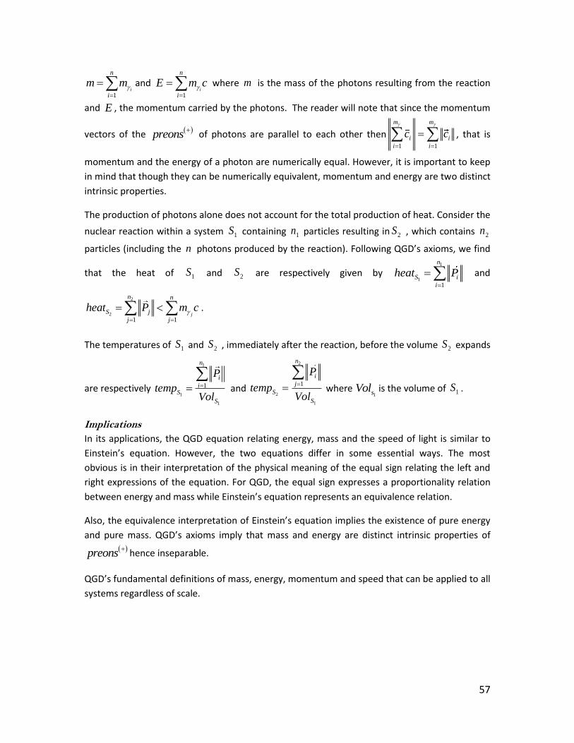
57
1i
n
i
m m
and 1
i
n
i
E m c
where m is the mass of the photons resulting from the reaction
and E , the momentum carried by the photons. The reader will note that since the momentum
vectors of the preons
of photons are parallel to each other then
1 1
m m
i i
i i
c c
, that is
momentum and the energy of a photon are numerically equal. However, it is important to keep
in mind that though they can be numerically equivalent, momentum and energy are two distinct
intrinsic properties.
The production of photons alone does not account for the total production of heat. Consider the
nuclear reaction within a system 1S containing 1n particles resulting in 2S , which contains 2n
particles (including the n photons produced by the reaction). Following QGD’s axioms, we find
that the heat of 1S and 2S are respectively given by 1
1
1
n
S i
i
heat P
and
2
2
1 1j
n n
S j
j j
heat P m c
.
The temperatures of 1S and 2S , immediately after the reaction, before the volume 2S expands
are respectively
1
1
1
1
n
i
iS
S
P
tempVol
and
2
2
1
1
n
i
j
S
S
P
tempVol
where
1sVol is the volume of 1S .
Implications
In its applications, the QGD equation relating energy, mass and the speed of light is similar to
Einstein’s equation. However, the two equations differ in some essential ways. The most
obvious is in their interpretation of the physical meaning of the equal sign relating the left and
right expressions of the equation. For QGD, the equal sign expresses a proportionality relation
between energy and mass while Einstein’s equation represents an equivalence relation.
Also, the equivalence interpretation of Einstein’s equation implies the existence of pure energy
and pure mass. QGD’s axioms imply that mass and energy are distinct intrinsic properties of
preons
hence inseparable.
QGD’s fundamental definitions of mass, energy, momentum and speed that can be applied to all
systems regardless of scale.

58
Other Consequences of QGD’s Gravitational Interaction Equation
Dark Photons and the CMBR
Another implication of the axiom set of QGD which will be discussed in detail in the cosmology
section of this book follows what the initial state of the universe it predicts. In its initial state,
the only matter was in the form of free preons
which were isotropically distributed
throughout quantum-geometrical space.
During the isotropic state, preons
, as a consequence of the attractive force acting between
them and over long travelling distances, started to form the simplest of all particles; low mass
photons and neutrinos. And because preons
were distributed isotropically, so was the
distribution of these particles.
From the description of the laws of momentum, assuming that variations in gravity and the
electromagnetic are negligible, the permitted change in momentum permitted for an electron
must obey the relation e e
P xm 4. This means that photons (or neutrinos) whose
momentum e
P m are undetectable and therefore dark (we’ll refer to them as dark
photons).
If QGD’s is correct, then the first detectable photons, photons for which e
P m , have been
first observed in 1964 by Arno Penzias and Robert Wilson and correspond to the cosmic
microwave background radiation (CMBR). The observed isotropy of the CMBR then follows
naturally from the initial isotropic state of the universe.
Effect Attributed to Dark Matter
We will see in the section titled QGD Cosmology that the universe’s initial state was that
contained nothing but quantum-geometrical space and free preons
which were
homogenously distributed in space.
Under the effect of gravity, free preons
formed large structures. The effect we attribute to
dark matter is the interactions between light and material structures with regions of space in
which free preons
have condensed and which we call now dark matter halos.
4 The general equation is
e eP xm G where G and are respectively the
gravitational and electromagnetic effects acting on e
. The general equation will be discussed and
applied in the section Preonics (foundation of optics) .
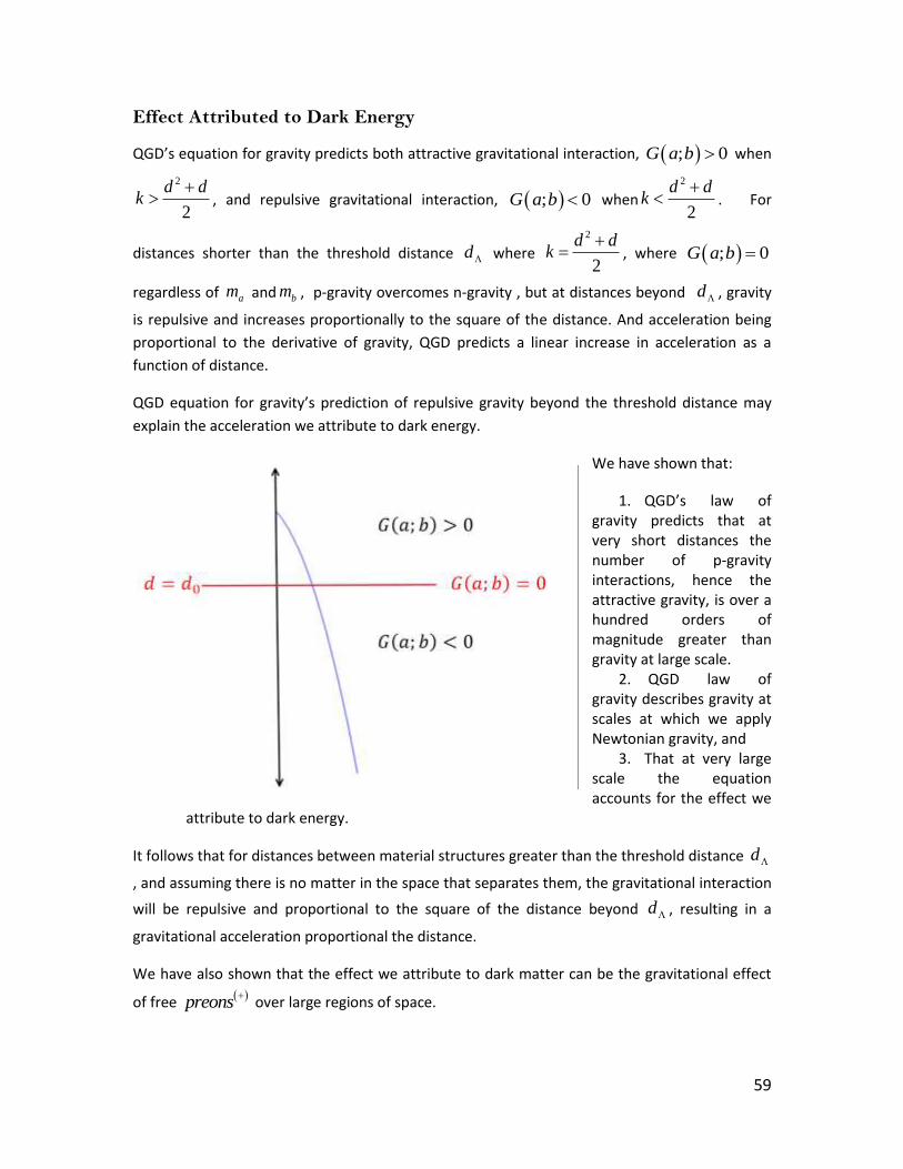
59
Effect Attributed to Dark Energy
QGD’s equation for gravity predicts both attractive gravitational interaction, ; 0G a b when
2
2
d dk
, and repulsive gravitational interaction, ; 0G a b when
2
2
d dk
. For
distances shorter than the threshold distance d where
2
2
d dk
, where ; 0G a b
regardless of am and bm , p-gravity overcomes n-gravity , but at distances beyond d , gravity
is repulsive and increases proportionally to the square of the distance. And acceleration being
proportional to the derivative of gravity, QGD predicts a linear increase in acceleration as a
function of distance.
QGD equation for gravity’s prediction of repulsive gravity beyond the threshold distance may
explain the acceleration we attribute to dark energy.
We have shown that:
1. QGD’s law of gravity predicts that at very short distances the number of p-gravity interactions, hence the attractive gravity, is over a hundred orders of magnitude greater than gravity at large scale.
2. QGD law of gravity describes gravity at scales at which we apply Newtonian gravity, and
3. That at very large scale the equation accounts for the effect we
attribute to dark energy.
It follows that for distances between material structures greater than the threshold distance d
, and assuming there is no matter in the space that separates them, the gravitational interaction
will be repulsive and proportional to the square of the distance beyond d , resulting in a
gravitational acceleration proportional the distance.
We have also shown that the effect we attribute to dark matter can be the gravitational effect
of free preons
over large regions of space.

60
Einstein’s Equivalence Principle
According to QGD, there is only one definition of mass: the intrinsic mass of an object being
simply the number of preons
it contains. The intrinsic mass determines not only the effect of
gravity but all non-gravitational effect.
The gravitational mass is that property which determines the magnitude of gravitational
acceleration while the inertial mass determines the magnitude of non-gravitational acceleration.
It is important in describing a dynamic system that we understand that the distinction made
between the gravitational and inertial masses are actually distinctions between gravitational and
non-gravitational effects. Doing so, we will show that the intrinsic mass determines both
gravitational and non-gravitational effects and that these effects are very distinct, thus
distinguishable.
The acceleration of an object is given by a
a
a
Pv
m
where aP G for gravitational
acceleration and aP F for non-gravitational force F imparting momentum to a . From
2 2 2 2
1 1 2 2 1 1 2 21
2 2 2 2a a b b
a a
G d d d d d d d dv m m k k m k k
m m
we know that gravitational acceleration is independent of the mass of the accelerated body,
while a
a
Fv
m tells us that non-gravitational acceleration is inversely proportional to the
mass of the accelerated body.
Let us consider the experiments represented in the figure below which based on Einstein’s
famous thought experiment.
61
The green rectangles represent a room at rest relative to Earth’s gravitational field.
The Earth and green room dynamics is described by the equationg
gg
P Pv v
m m
where g represents the green room and the Earth. Applying the laws of momentum
discussed earlier, we know that green room and the Earth are moving at the same speed hence,
since 0g g
v v m
and 0g
v v m there is no momentum transfer between the
Earth and the green room, consequently no non-gravitational acceleration. And since there is no
change in distance between g and , there is no variation in the gravity, so no gravitational
acceleration either.
The red room is in region of space where the effect of gravity is negligible. A non-gravitational
force imparts momentum F to the red room from the floor up.
Einstein’s thought experiment assumes that it is possible to apply a force which will accelerate
the red room so that, to an observer within the room, the acceleration will be indistinguishable
from that of gravity. That is, He assumes that F G .
Before going into a full description of the experiment, we need to keep in mind the distinctions
between gravitational acceleration and non-gravitational acceleration. For one, gravitational
acceleration of body is independent of its mass while non-gravitational acceleration of a body is
inversely proportional to its mass. That is: F a F
a
a
v v mv
m
where Fv is the speed of the
particles carrying the momentum F (in the case of a rocket engine, this is the speed of the
molecules of gas produced by the engine which interact with the room) and av the speed of the
room. It follows that we can set F G for a given am but for an object of mass b am m
, we
can have F G but F F and F a F bF F
a b
a b
v v m v v mv v
m m
. Which means
that, to maintain an acceleration equivalent to gravitational acceleration, F must be adjusted
to take into account the mass of the accelerated to compensate for its speed since the imparted
momentum of a rocket engine (or any other form of propulsion) decreases as the speed
increases.
Returning to experiment 4, the green and red rooms will have the same mass and composition.
In each room, there will be a set of two spheres of mass am and bm where a bm m . In the
rooms initial state the spheres are suspended from rods fixed to the ceilings. The spheres can be
released on command. In each of the room is an observer that is cut off from the outside world.

62
They have no clue as to which of the two rooms they are in. The observers however, being
experimental physicists, are trusted to measure the accelerations of the spheres in the two
experiments and see if they can determine whether the room each is in is at rest in a
gravitational field or uniformly accelerated.
In the first experiment, the spheres with mass am will be dropped in each room. In the second
experiment, from the same initial state, spheres with mass bm will be dropped.
The green room observer finds that both spheres have the same rate of acceleration relative to
the room despite having different masses. He finds this to be consistent with gravitational
acceleration, but cannot exclude on these two experiments alone that he may be in a uniformly
accelerated room.
The red room observer however finds that rate of acceleration of the a sphere is lower than
the rate of acceleration of the more massive b sphere. His observations of the accelerations of
the spheres being inconsistent with gravitational acceleration he must conclude that the room is
accelerated by an external non-gravitational force F .
Furthermore, being a physicist, the red room observer knows that at the moment a sphere is
released, the momentum imparted by F is no longer transferred to the sphere. The sphere
stops accelerating instantly and will move at the speed it had at the moment of its. Therefore, it
is the room that is accelerated and not the sphere. The acceleration of the red room in its initial
sate is r
a br
Fv
m m m
. At the moment the a sphere is released, there is a sudden
change in the rate of acceleration of the room given by r
b a br r
F Fv
m m m m m
. The
change the rate of acceleration after the release of sphere b is
r
a a br r
F Fv
m m m m m
. The higher variation the in the rate of acceleration after
the release of b is seen from within the room as a larger acceleration of b relative to the
room.
So, it appears that observers can easily distinguish between being in a room at rest in a
gravitational field from being in a uniformly accelerated room away from any significant
gravitational field. This appears to invalidate the weak equivalence principle. Being an
experimental physicist, the observer in the red room requires confirmation of his observation.
He decides to repeat the experiment. After all, one experiment is not enough and one has to be
able to reproduce the results before doing something so drastic as to refute the weak
equivalence principle.

63
Again the more massive sphere accelerates faster than the lighter sphere, but something is
different. The acceleration rates of sphere a and sphere b in the second set of experiments are
slower than the accelerations of the same spheres in the first set of experiments. After
conducting a few more experiments he finds the observations to be consistent with
F Fr rP v v m and concludes that the momentum imparted by the non-gravitational
force decreases as speed of the room increases which allows him to predict that the maximum
possible speed the red room can achieve is Fr
v v at which speed 0F Fr r
P v v m
and 0r
r
r
Pv
m
.
If experiments confirm QGD predictions that:
Gravitational acceleration and non-gravitational acceleration are not equivalent then o Einstein’s equivalence principle is falsified
The outcome of an experiment may be affected by the speed of the laboratory then o The strong equivalence principle is falsified
Weightlessness in Einstein’s thought Experiment
Consider a man standing in an elevator when suddenly the elevator cable breaks. After the
rupture of the cable the elevator and the
passenger and elevator are in free fall and,
as if gravity had been turned off, they are
weightless.
There is, it seems, no acceleration; an
interpretation that is supported by the fact
that if we were to put an accelerometer on
the floor of the elevator, it would measure
no acceleration. In fact, an accelerometer
alone in free fall measures no acceleration.
In the absence of other forces (assumed to
be inexistent for the experiment) zero
acceleration implies that zero force and a
logical interpretation would be that gravity
is not a force. This interpretation leads to
the idea that gravity is the effect of
curvature of space-time.
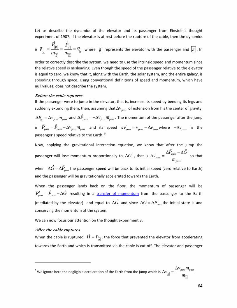
64
Let us describe the dynamics of the elevator and its passenger from Einstein’s thought
experiment of 1907. If the elevator is at rest before the rupture of the cable, then the dynamics
is g
gg
P Pv v
m m
where g represents the elevator with the passenger and . In
order to correctly describe the system, we need to use the intrinsic speed and momentum since
the relative speed is misleading. Even though the speed of the passenger relative to the elevator
is equal to zero, we know that it, along with the Earth, the solar system, and the entire galaxy, is
speeding through space. Using conventional definitions of speed and momentum, which have
null values, does not describe the system.
Before the cable ruptures
If the passenger were to jump in the elevator, that is, increase its speed by bending its legs and
suddenly extending them, then, assuming thatpassv of extension from his the center of gravity,
pass passP v m
and pass pass passP v m . The momentum of the passenger after the jump
is pass pass pass passP P v m and its speed ispass pass passv v v where
passv is the
passenger’s speed relative to the Earth. 5
Now, applying the gravitational interaction equation, we know that after the jump the
passenger will lose momentum proportionally to G , that is pass
pass
pass
P Gv
m
so that
when passG P the passenger speed will be back to its initial speed (zero relative to Earth)
and the passenger will be gravitationally accelerated towards the Earth.
When the passenger lands back on the floor, the momentum of passenger will be
pass passP P G resulting in a transfer of momentum from the passenger to the Earth
(mediated by the elevator) and equal to G and since passG P the initial state is and
conserving the momentum of the system.
We can now focus our attention on the thought experiment 3.
After the cable ruptures
When the cable is ruptured, g
H P , the force that prevented the elevator from accelerating
towards the Earth and which is transmitted via the cable is cut off. The elevator and passenger
5 We ignore here the negligible acceleration of the Earth from the jump which is
pass passv mv
m
65
will move at their initial speed towards the Earth that is g
g
g
Pv
m . What the passenger
perceives as weightlessness is correct. Since the weight is simply the measurement of H , when
the cable is cut off, H is no longer imparted to the passenger and thus he is weightless. The
removal of the effect of weight is not the removal gravity but the removal of the force that
opposes gravity. There is increase in momentum, hence acceleration, which the passenger will
be transferred to the Earth when the elevator hits the ground.
Since all components of an accelerometer are accelerated uniformly and at the same rate (see
universality of free fall) it cannot measure gravitational acceleration. What an accelerometer
measures is the effect of weight. That is: it measures H . And H ceases to be transferred to the
elevator and content after rupture of the cable so it will measure zero weight.
However, though the accelerometer ( denoted acc below ), cannot measure gravitational
acceleration, it can inform of its momentum, its gravitational acceleration and its speed if we
record and correctly interpret the measurement it makes before release, the null reading
during free fall, the measurement at impact and after impact since:
accH P accP
,
G and acc
acc
Gv
m
, and
accH P accP .
If there were a second elevator cabin was in space and moving at uniform speed, as describe in
another one of Einstein thought experiment, it would be in a state of weightlessness and
without gravity, so that 0 . That would allow an observer to easily distinguish the
experience of being in a cabin in space from being in a cabin free falling in a gravitational field.
What we have shown that though there is only one kind of mass, the effects of gravity and non-
gravitational force can never be equivalent. And even when cut off from the outside world, as is
imagined in Einstein’s thought experiments, observers can correctly describe and distinguish
between the forces acting on their environment through experiments as long as measurements
are made of the initial, transitory and final states of the experiments and a minimum of two
distinct experiments are conducted for each measured property.

66
Gravitational Waves or the Elephant in Room
QGD precludes the existence of gravitational waves so how can this be reconciled with the
advanced LIGO observatory detections of signals that are consistent with gravitational waves
predicted from general relativity? How does QGD explain these signals if, as it predicts, there are
no gravitational waves?
LIGO made detected several signals that were thought to be due to gravitational waves but only
the detection of the event known as GW170817 had electromagnetic counterparts. This
observation makes it possible to narrow down the possible explanations to one.
If QGD’s theory of gravity is correct then the observations of electromagnetic counterparts
rather than confirming the existence of gravitational waves falsifies it. Or at the very least
excludes the possibility that GW170817 is a gravitational signal. The question we must then
answer is: What explains the signal?
It is important to keep in mind that any explanation we provide must be consistent with QGD’s
axiom set. The axiomatic approach adopted for QGD prohibits the introduction of ad hoc
explanations in the theory.
First, since LIGO-VIRGO detected the GW170817 only 1.7 seconds before the detection of a
gamma ray burst GRB170817, if the signal was generated by the same event we can assume that
it must have travelled at the speed of light. Now, according to QGD, only preons
, photons
and neutrinos can travel at the speed of light. Since GW170817 is neither of the latter two we
are left with only one possibility; GW170817 is caused by preons
, specifically
preons
resulting from the polarization of a large regions of the preonic field. The mechanism of
polarization has been discussed in detail here.
Secondly, the event produces a wave-like signal which increases in both frequency and
amplitude. This is consistent with the polarization of the preonic field by a coalescing binary
system.
As the stars of a binary system accelerate towards each other, they themselves become
polarized. The polarization of the stars results from the polarization of the components
preons
of the stars by the increasing gravitational interaction in accordance to the laws we
derived in the section titled Gravitational Interactions and Momentum.
The intensity of the polarization of the preonic field is by each one of the stars proportional to
the size and density of the stars and its rotation speed.
For a binary system, the polarization of a neighboring region of the preonic field will vary as
polarized stars pass through them. So the closer there orbit each other, the higher the orbital
speed, the greater the frequency. And the greater their speed, the greater their polarization.
67
The frequency of the signal is the proportional rotation speed of the binary system v
f
As for the amplitude of the signal P we have
1 1 2 2
cos coscos
b b b bp pP dens dens P dens dens
P vd
where sv is the
rotation speed of the system, is the angle of the star relative to the line of sight, is the
inclination of the plane of rotation, d the distance of the observer, and 1b
dens and 2bdens are
the density of the stars 1b and 2b .
From the above, we can see that the signals detected by LIGO and VIRGO are consistent with
both the prediction of general relativity and QGD, that is it could cause by gravitational waves or
by preonic waves. Thus a prediction unique to QGD is necessary to determine which of the
interpretations of the observations is correct.
Preonic waves are composed of polarized preons
just as magnetic fields are. It follows that if
the signal is due to preonic waves, QGD predicts that it would cause fluctuations in the magnetic
moment of a magnet and the signal formed by the fluctuations will mirror the signal detected by
LIGO-VIRGO observatories or other gravitational wave detector. Testing the prediction requires
high precision magnetic field sensors to monitor the fluctuations in the magnetic fields
generated by reference magnets and simultaneously comparing them to signals detected by
LIGO-VIRGO or future detectors

68
Locality, Certainty and Simultaneity
Locality and Instantaneous Effects
Non-locality is based on the assumption that an event which affects a system cannot affect
another system which is independent of it. Independent systems being defined as systems
which are separated by a distance sufficiently large to prohibit one from influencing the other
without violating the speed limit predicted by special relativity. But if gravity is instantaneous,
then no systems is truly independent which means that all systems are local and can affect each
other instantaneously regardless of distance.
Under instantaneous interactions, the entire universe is local.
Currently, independent experiments which show correlations that cannot be accounted for by
local hidden variables correlation are taken as evidence that reality is fundamentally non-local,
hence are taken as evidence supporting quantum-entanglement. But if gravitational
interactions and the electromagnetic effect of generation of magnetic fields are instantaneous,
then any two experiments will influence each other instantaneously yet remain classical since
they do so without violating locality since, as we have indicated earlier, the entire universe
becomes local if these effects are instantaneous.
Instantaneity and the Uncertainty Principle
The uncertainty principle states that two conjugate properties cannot be known with certainty.
The most common example being that of the properties of momentum and position. According
to the Heisenberg’s uncertainty principle, as the certainty of the measurement of momentum
increases, the uncertainty of the position increases as well. This is described by the famous
equation 2
x p and thought to be inherent to wave-like systems. But if space is discrete
(quantum-geometrical as per QGD’s axiom of discreteness of space), then the wave function
provides only an approximation of the scattering of singularly corpuscular particles and the
uncertainty principle is a consequence of quantum mechanics; one that does not correspond to
a fundamental reality in which space is discrete rather than continuous.
Position and Momentum of Particles (or Structures)
Consider a particle which momentum and position are unknown and two gravitational detectors
as shown in figure 1. The red circles in the figure represent arrays of photon detectors which will
detect and measure the photons energy and direction.
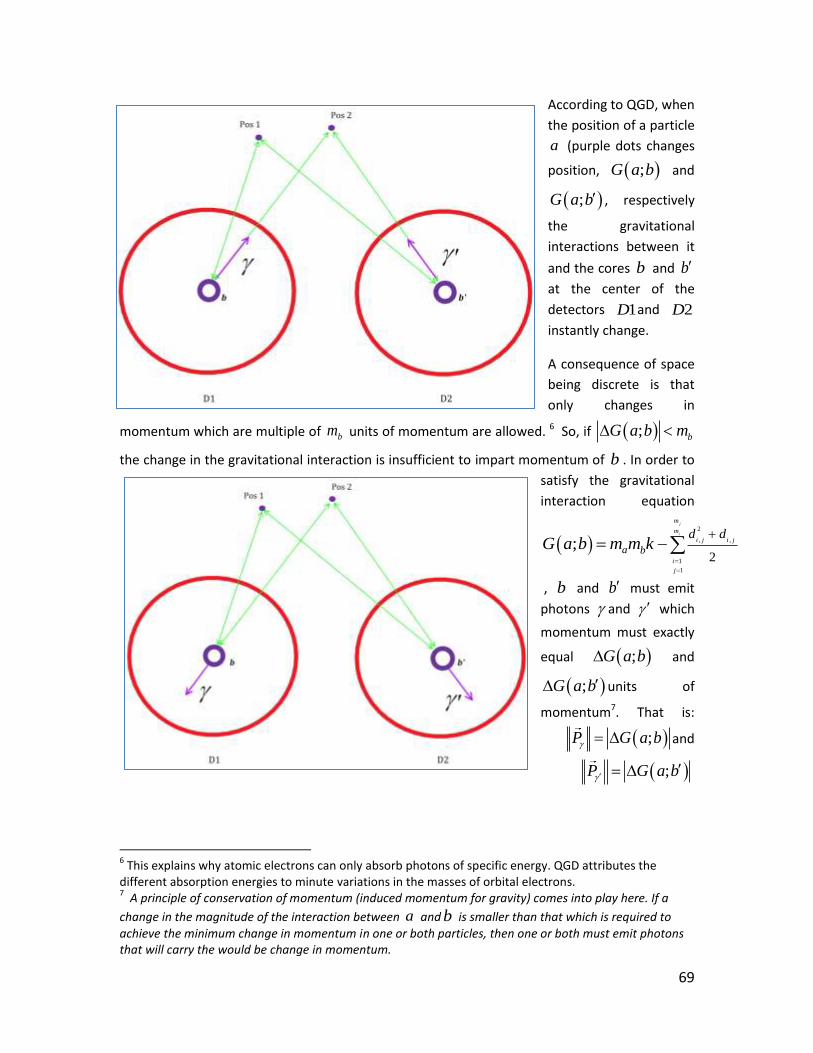
69
According to QGD, when
the position of a particle
a (purple dots changes
position, ;G a b and
;G a b , respectively
the gravitational
interactions between it
and the cores b and b
at the center of the
detectors 1D and 2D
instantly change.
A consequence of space
being discrete is that
only changes in
momentum which are multiple of bm units of momentum are allowed. 6 So, if ; bG a b m
the change in the gravitational interaction is insufficient to impart momentum of b . In order to
satisfy the gravitational
interaction equation
2
, ,
1
1
2;
j
i
m
m
i j i j
i
j
a b
d dG a b m m k
, b and b must emit
photons and which
momentum must exactly
equal ;G a b and
;G a b units of
momentum7. That is:
;P G a b and
;P G a b
6 This explains why atomic electrons can only absorb photons of specific energy. QGD attributes the
different absorption energies to minute variations in the masses of orbital electrons. 7 A principle of conservation of momentum (induced momentum for gravity) comes into play here. If a
change in the magnitude of the interaction between a and b is smaller than that which is required to
achieve the minimum change in momentum in one or both particles, then one or both must emit photons that will carry the would be change in momentum.

70
where the directions of the momentum vectors P and P (purple arrows) coincide with
;G a b and ;G a b .
By triangulation, the instantaneous position and distance of a can be found and depending on
the distance and direction we can make the following interpretation:
1. If distance is such that 2
2
d dk
and P points towards a , then a is moving
towards b ;
2. If 2
2
d dk
and P (or P ) points away from a then a is receding from b ;
3. If 2
2
d dk
and P points towards a , then a is receding from b ;
4. If 2
2
d dk
and P points away from a , then a is moving towards b .
The momentums (which for photons is equal to their energy) P and P provides an exact
measure of ;G a b and ;G a b . Since bm and bm are known, we can resolve the
gravitational interaction equation for am , hence obtain an exact value of its mass.
Thus a first measurement gives us the instantaneous position and mass of a .
A second measurement with give us a second position, hence the distance travelled between
position 1 and position 2. This allows us to calculate speed xa
ref
dv c
d were
refd is the distance
light would have travelled during the same interval. From QGD’s definition of speed we know
that a
a
a
Pv
m where
aP is the momentum vector of a so that a a aP m v . Therefore, a
second measurement allows us to find simultaneously the position and momentum of a with
certainty.
Position and Momentum of Charged Particles
In the above description, we assumed that the particle was electrically neutral. If the particle is
not neutral, then QGD predicts the generation of a magnetic field is instantaneous and the
same reasoning applies with the difference that in addition to changes in gravitational

71
interactions, we have changes in the intensity of the magnetic field and the momentum they can
impart to b and b .
Here again, when bH bP m , the structures b and b must emit photons and where
bHP P andbHP P . In the case of charged particles, the change momentum
imparted by a magnetic being orders of magnitude greater than the change in momentum
imparted by gravity, the photons and will have momentums orders of magnitude greater
than that of photons produced from variations in the gravitational interactions alone.
Two measurements using the apparatus in Figure 1 for a charged particle will simultaneously
provide its instant position and momentum with certainty.
Interactions between Distant Experiments
If space is discrete as per QGD’s axiom, then we know that there can be significant differences
between the geometrical distance and the physical distance between any two positions in
space. The physical distance between two particles, even when large, may be significantly
reduced even by a small
shift in their positions.
In the figure on the left, the
geometrical distance may
be associated with the
lengths of the red arrows,
while the physical distance,
corresponds to the number
of the number of leaps
necessary to move from an
initial position (green circle)
to a second position (blue
circles).
As we can see, though the geometrical distances between the green position and the blue
positions may vary greatly, the physical distance between them is the same and equal to one
unit.
In the figure on the left, we see
that at the fundamental scale,
Pythagoras’s theorem does not
hold. How Euclidean space
emerges at larger scales is
explained in here. If we assume
the existence of a particle b

72
positioned at the top vertex and particle a at the bottom left vertex (green circle). If a moves
one position to the right to the bottom right vertex, the physical distance between a and b
becomes four times smaller even though the geometrical distance increased. Such changes in
physical distance will cause significant instantaneous changes in the gravitational interaction
between the particles and additionally, if the particles are not electrically neutral, significant
changes the magnetic field they generate.
Since experiments use electronic components, they contain particles or structures a and b
which are not electrically neutral. In such case, the change in the momentum of the magnetic
field they generate can impart will be orders of magnitude greater than that of purely
gravitational changes and photons emitted by b will have significantly greater energy.
When in one experiment a particle is measured, it causes changes in the momentum of some of
its component particles (changes in electrons within the electrical current which powers its
detectors for example), these changes are compounded and will cause components of a second
experiment to emits photons instantly. Some of the photons produced within the second
experiment will have energies in the range of the sensitivity of detectors.
The Notion of Simultaneity
As we have explained, if gravity is instantaneous then all objects in the universe are local. That
means that if an event affects an object anywhere in the universe, the gravitational interactions
between that object and all other objects in
the universe regardless the distances that
separate them will be affected instantly.
An event can be defined as a change in mass,
density, direction, speed, momentum or
position, all of which affect either the
magnitude and/or direction of the
gravitational interaction between the object
of the event and all others objects in the
universe.
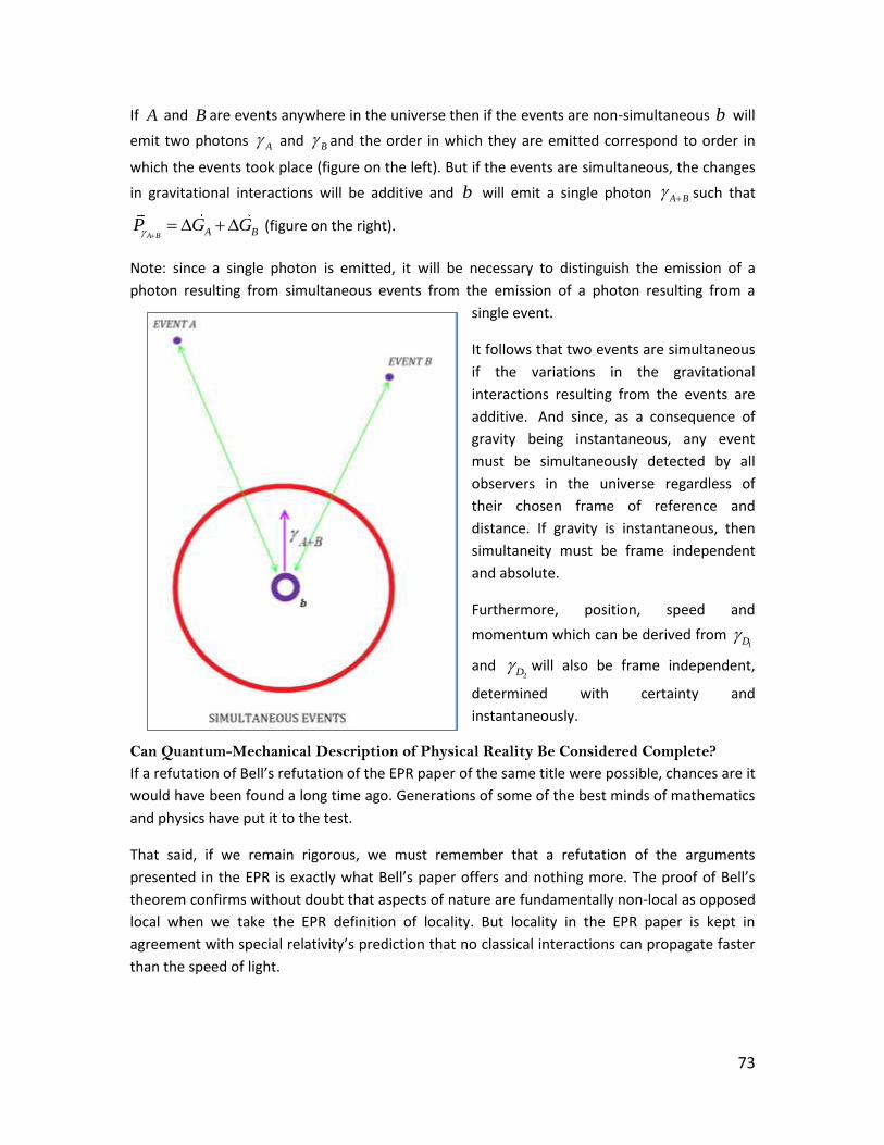
73
If A and B are events anywhere in the universe then if the events are non-simultaneous b will
emit two photons A and B and the order in which they are emitted correspond to order in
which the events took place (figure on the left). But if the events are simultaneous, the changes
in gravitational interactions will be additive and b will emit a single photon A B such that
A B A BP G G (figure on the right).
Note: since a single photon is emitted, it will be necessary to distinguish the emission of a
photon resulting from simultaneous events from the emission of a photon resulting from a
single event.
It follows that two events are simultaneous
if the variations in the gravitational
interactions resulting from the events are
additive. And since, as a consequence of
gravity being instantaneous, any event
must be simultaneously detected by all
observers in the universe regardless of
their chosen frame of reference and
distance. If gravity is instantaneous, then
simultaneity must be frame independent
and absolute.
Furthermore, position, speed and
momentum which can be derived from 1D
and 2D will also be frame independent,
determined with certainty and
instantaneously.
Can Quantum-Mechanical Description of Physical Reality Be Considered Complete?
If a refutation of Bell’s refutation of the EPR paper of the same title were possible, chances are it
would have been found a long time ago. Generations of some of the best minds of mathematics
and physics have put it to the test.
That said, if we remain rigorous, we must remember that a refutation of the arguments
presented in the EPR is exactly what Bell’s paper offers and nothing more. The proof of Bell’s
theorem confirms without doubt that aspects of nature are fundamentally non-local as opposed
local when we take the EPR definition of locality. But locality in the EPR paper is kept in
agreement with special relativity’s prediction that no classical interactions can propagate faster
than the speed of light.

74
It follows that Bell’s paper may also be taken as a refutation of locality as derived from special
relativity or even as a refutation of special relativity’s prediction precluding faster than light
interactions.
As we have seen, QGD distinguishes between propagation which is the motion of particles or
structures which speed cannot exceed the speed of light, gravitational interactions which is
instantaneous and without mediating particles8 and non-gravitation interactions which implies
absorption and/or emission of particles and transfer of their momentum. It follows that non-
gravitational interactions are limited to the speed of light.
Implications for Bell Type Experiments
If classical forces and quantum entanglement both violate locality as it is described in the EPR
paper and which description assumes that no classical force can propagate faster than c , then
how can we know whether a violation of Bell's inequalities is due to a classical or to a quantum
mechanical effect? Would this render the proof of Bell’s theorem via the violation of Bell’s
inequality irrelevant? Or should it be taken as taken not as a refutation of the EPR locality, but
of the understanding and description of locality it assumes?
If any observed violation of Bell’s inequality could attributed to instantaneous classical effects
Bell-type experiments would no longer allows us to distinguish between the two.
It would however be possible to determine if such violation is caused by classical instantaneous
interactions since realism would be preserved and, as we have shown above, we could
simultaneously and with certainty measure conjugate properties such as momentum and
position; something that would not be possible if reality was quantum mechanical.
On the Effect of Gravitational Interactions on Particle Decay and how
it Can be Used for Gravitational Telescopes
In figure 1, if b and b are massive nuclei such that ; bG a b m and ; bG a b m ,
then b and bwill emit particles x and x for which ;xP G a b and ;xP G a b
respectively. So if x and x are simultaneously emitted (and detected by the array) and
their directions converge, then there is a probability that their emissions result from the a
change their gravitational interactions between b and b and a . But when considering that
all matter in the universe interacts, the convergence of the directions of the particles
emitted by b and bonly means that the objects they interact with are somewhere along the
directions of their emitted particles and that the changes in gravitational interactions are
simultaneous. For a gravitational telescope that exploits the effect we described requires
that this probability be significantly increased.
8 According to QGD, particles do not mediate forces. They can, as in magnetic fields, impart momentum to
particles or structures.

75
This could be done by
augmenting the number of
massive nuclei of the
apparatus. If n is the number
of massive nuclei so that
;ii bG a b m where i n ,
then we can predict n
simultaneously emitted
particles ix which have the
predicted momentum and
which directions converge onto a sufficiently small region of space, then for a certain value
of n the probability that the simultaneous emission of particles result from the nuclei’s
gravitational interactions with a approaches certainty. That is, the number of possible
objects which would cause the observation is reduced to 1.
A gravitational telescope exploiting the effect can thus discriminate precisely between the
objects it observes and provide their position, momentum and mass with certainty.
Note: The type of particles emitted by nuclei will depend on the strength of the bonds between
the particles when they were components of the nuclei, their masses as well as the magnitude
of the variation in the gravitational interactions. Since, as shown earlier, even small changes
in position can cause disproportionately large changes in the physical distance between
objects, they induce emissions of particles with significantly greater momentum than would be
possible if space were continuous.
Note: The effect described in this section may already have been observed. See Evidence for
Correlations Between Nuclear Decay Rates and Earth-Sun Distance by Jere H. Jenkins, Ephraim
Fischbach, John B. Buncher, John T. Gruenwald, Dennis E. Krause, Joshua J. Mattes.
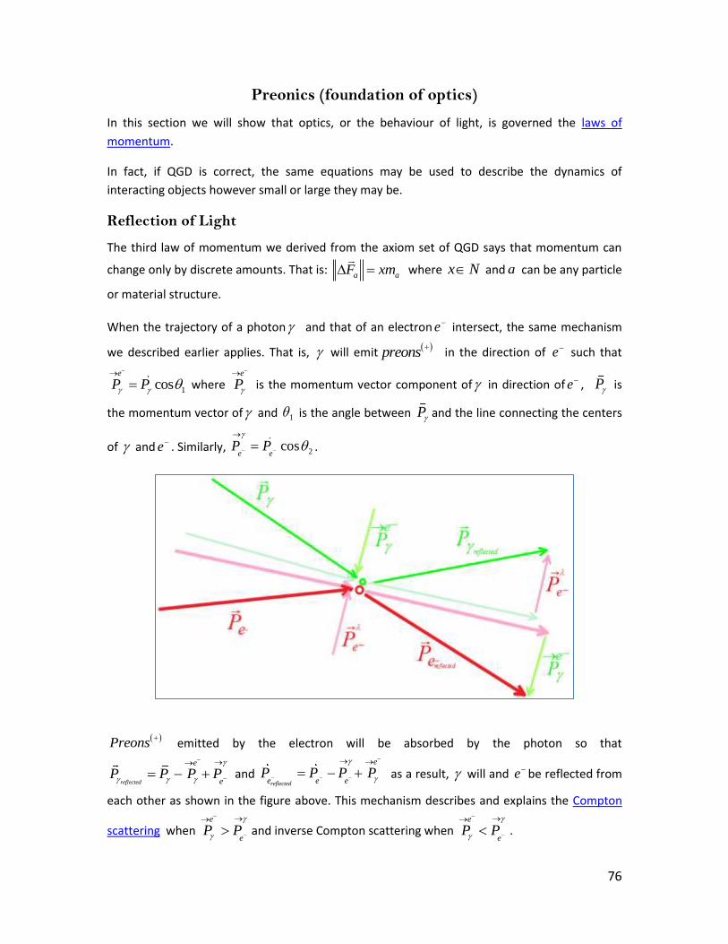
76
Preonics (foundation of optics)
In this section we will show that optics, or the behaviour of light, is governed the laws of
momentum.
In fact, if QGD is correct, the same equations may be used to describe the dynamics of
interacting objects however small or large they may be.
Reflection of Light
The third law of momentum we derived from the axiom set of QGD says that momentum can
change only by discrete amounts. That is: a aF xm where x N and a can be any particle
or material structure.
When the trajectory of a photon and that of an electron e intersect, the same mechanism
we described earlier applies. That is, will emit preons
in the direction of e such that
1cose
P P
where e
P
is the momentum vector component of in direction of e , P is
the momentum vector of and 1 is the angle between P and the line connecting the centers
of and e . Similarly, 2cose e
P P
.
Preons
emitted by the electron will be absorbed by the photon so that
reflected
e
eP P P P
and reflected
e
e e eP P P P
as a result, will and e be reflected from
each other as shown in the figure above. This mechanism describes and explains the Compton
scattering when e
eP P
and inverse Compton scattering when e
eP P
.

77
The Electromagnetic Effects of Attraction of Repulsion
The preonic field is composed of free preons
uniformly distributed in quantum-geometrical
space. Free preons
interact with particles or structures matter in accordance to the laws of
momentum which as we have seen govern preonics of which is a generalization of optics. When
interacting with a particle or structure, preons
are absorbed and emitted following the
structure of the particle or structure. When the components of a particles or structures are
random, the absorbed and reflected preons
are also random so that the momentum of the
neighbouring preonic field is equal to zero. That is: 1
0m
i
i
P c
.
However when the
components of the
particle or structure
(electrons for example)
are aligned in which case
the absorbed and
reflected preons
will
consequently be aligned. Such particles or structures which components motions are aligned are
called charged. The interactions between the preonic field and a charged particle or structure
cause the polarization the preonic field which we call the magnetic field. From the discussion
about optical reflection we know that the direction of the reflection will depend on the direction
of the particles the preons
will interact with. The figure above is a diagram that shows the
dependency of the reflection of preons
on the orientation of a particle or structure. The black
vectors represent the direction of the components of the particles or structures a and a , and
the blue vectors represent the polarization of the preonic field in the regions neighbouring
them.

78
When two charged particles or
structures come into proximity, they
each interact with regions of each
other’s polarized preonic field. The
figure on the left shows how we will
represent and label charged particles
or structures and the interacting
regions of the polarized preonic field.
Compton Scattering and the Repulsion and Attraction of Charged Particles.
We have shown in the section on reflection of light that when applying the laws of momentum
to the interaction between photons and atomic electron that the Compton scattering occurs
when e
eP P
and the inverse Compton scattering when e
eP P
where is the incident
photon and e
P
and e
P
are respectively the momentum of the preons
emitted by the
electron and the momentum imparted by the photon with which it interacts. Conservation of
momentum requires that the momentum of the electron must change by a vector of equal
magnitude but inverse direction of the sum of e
P
and e
P
. That is, e
e eP P P
. This
implies that if e
eP P
then the momentum vector of the electron will increase in the direction
opposite of the point of interaction bye
P . Inversely, if e
eP P
then the electron’s
momentum vector will increase towards the point of interaction by e
P . Whether we have a
Compton or reverse Compton scattering depends on the relative direction of the photon and
electron (or particle or structure). That is, based on the laws of momentum, if the photon and
electron at the point of interaction move directly towards each other, then e
eP P
and if
their trajectories intersect tangentially, then e
eP P
. The Compton scattering and its inverse
are special cases of preonic interactions which can explain the effects of repulsion and attraction
of charged particles.

79
ATTRACTION EFFECT
Polarization Interaction Inverse Compton
The figure on the left illustrates
the interaction between two
oppositely charged particles (
a and a ) . The circular
vectors represent the angular
momentum of the particles and
the blue and red vectors
correspond to the direction of
the polarization preonic field
respectively. Since the
polarization of 1a
is
opposite to orientation of 2a
then 2
2
1
1
a
a
a
aP P
and 2a
P
will point away from 1a
,
thus 2a will move away from
1a . Similarly, the polarization of 2a
is opposite the
orientation of 1a so that
2
2
1
1
a
a
a
aP P
, consequently 1a will move away from
2a . This
explains the effect of repulsion between two similarly charged particles (and structures).
In the figure on the right, we have
to particles of opposing charges.
Here since the polarization of the
region a
is opposite to the
orientation of a and the region
a
is polarized in opposite the
orientation of a then
a
aa
aP P
and
a
aa
aP P
and as a result a
P will point to
a and a
P will point to a .
Therefore a and a will move
towards each other and appear to
REPULSION EFFECT
Polarization Interaction Compton

80
be attracted.
As we shown, the observed repulsion between like charges and attraction between opposite
charges does not result from repulsion and attraction between the particles themselves but
from their interactions between the preonic regions polarized by other particles.
Also, since the polarized preons
are emitted radially from a charged particle or structure, the
intensity or momentum of the polarized region follows the inverse square law. In fact the
inverse square law of the momentum of a magnetic field is a consequence of QGD’s preonics.
Interaction between Large Charged Structures and the Preonic Field
Large structures that have aligned charged particles behave in the way we have described in the
preceding section. The main difference is that the effect of a large number of aligned charged
particles creates more intense polarization over a much larger region of the preonic field.
The intensity of the magnetic field at a distance r from a charged structure is
2r
dens a densS aP
r
where dens is the density of the preonic field or dens
m
vol
, aS is the
surface of the interacting particle or structure (its cross section) and densa is the density of
aligned electrons on the surface of a .
Note: In a following section, we will discuss how the dynamics of atomic electrons follow from
QGD’s laws of momentum.

81
Refraction of Light
Changes in momentum of an electron are discrete increments proportional to its mass, that is,
e eP m
.
Now consider a photon 0 interacting with an atomic electron with 1e
e exm P x m
wheree
P
is the momentum vector of the photon emitted by 0 in direction of e as a
component of the interaction as we explained earlier, ande
eP P
.
To be consistent with the laws of momentum transfer, 0
0
e
e e e
PP m
P
so upon absorption of
the
preons
emitted by 0 the electron must emit a photon 1 such that 1 0 e
P P P
(see figure below). This is the basic mechanism of refraction.
From the equation, we see that 0 , the angle between 0 and 1 (angle of refraction), is
inversely proportional to0
P . That is, the greater the momentum (which corresponds to higher
energy or higher frequency in accepted physics), then the greater the refraction for a single
interaction. But the refraction of light, by a prism for example, is the result of a series of
interactions.
That is: since 0
1e
e exm P x m
, then for 1i x we have i
e
eP m
and
1i iP P
and as a consequence 0i . So there is no refraction for photons once

82
i
e
eP m
. The point at which a photon achieves maximum refraction is directly
proportional to its momentum and this produces the colour separation by prism.
Note that the shape of the prism is ideal as it allows for photons of different momentums to
achieve maximum diffraction.
If the number of refractive interactions is lower than what is necessary for photons to achieve
maximum refraction, then the colours will be separated due to reflection and as we have seen,
the angle of reflection is smaller the higher the momentum is. That explains why refraction using
a grid is smaller for photons with higher momentums than photons with lower momentums.
Diffraction of Light
Diffraction is a simple consequence of reflection, that is, the interaction between light and
matter and not, as thought, between light waves.

83
The light bands of diffraction
patterns correspond to the allowed
changes in momentum of particles
or structures and the dark bands
correspond to the forbidden
changes in momentum.
The bands will appear if there is one
source of light and the photons
composing the light are have similar
momentum. Applying our
understanding of reflection of light,
we find that the reflection angle of
a photon depends not only on its
angle of incidence but also on its
momentum. The smaller the angle,
the smaller will be the momentum
from the electron it interacts with
and the smaller will the momentum
and angle of reflection of the reflected photon. The angle of reflection of a photon is close to but
not equal to the incident angle.
In a strict description the reflection, we must also consider that that only certain changes in
momentum are allowed as per our description of momentum and momentum transfer we saw
here. So if e
P
is the momentum emitted by the electron in direction of the photon with
which it interacts and if 1e
xm x mP
, then P xm so that all photons within a
range of incident angle will be reflected at the same exact angle, but that none will be reflected
at angles in the between the exact angle of reflection (this is only true of course for photons of
the same momentum). The result will be as described in the figure above.
The width between the bands but is proportional to difference between the allowable momentums changes they correspond to given a slit of the same depth and width. As for the number of dark fringes,
we will show in the next section
that it is proportional to the
number of allowed changes in

84
momentum within the angles of diffraction permitted by the aperture. That is:
maxcos2fringes
e
Pn
m
where max is half the aperture angle and fringesn is the number dark
fringes on the x or y axis.
As for the pattern of diffraction, it will depend on the shape of the aperture. Applying the
equations we have introduced we can predict the patterns generated by a group of photons.
Fringe Patterns from Double-slit Experiments
Following the failure of classical physics theories to explain the interference patterns observed
in double slit experiments and other light diffraction experiments and because of the similarities
between these patterns and the interference
patterns generated by waves at the surface of a
liquid, physicists deduced that light was
behaving as a wave which led to the so-called
wave-particle duality of light. Since the particle
model could explain phenomena such as the
photoelectric effect and since the wave model of
light described the interference patterns of light,
it made sense to deduce that light had to
corpuscular or wave-like depending on the
experiment performed on it. But what
experiments actually showed is that neither
accepted models of light could explain both
behaviours and emphasized the need for a new
theory.
The patterns generated in double-slit experiment are thought to be the results of interferences
between light waves, but they can be better understood in terms of the reflection and
absorption patterns of photons through a mechanism consistent with the laws governing optics
(or more generally, preonics) .
Though we describe the double-slit experiments that use photons, the same explanation applies
for electrons or any other particle.
Single Slit Experiment
We will first describe single slit experiments.
The momentum vector components that can be imparted to an electron is given by cosP
where is the angle between the P and e
P , but from the laws of momentum we know that
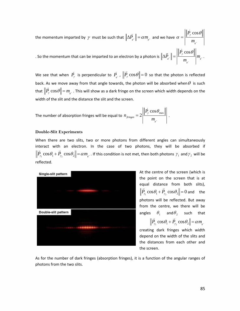
85
the momentum imparted by must be such that e e
P m and we have cos
e
P
m
. So the momentum that can be imparted to an electron by a photon is cos
e e
e
PP m
m
.
We see that when P is perpendicular to e
P , cos 0P so that the photon is reflected
back. As we move away from that angle towards, the photon will be absorbed when is such
that cose
P m . This will show as a dark fringe on the screen which width depends on the
width of the slit and the distance the slit and the screen.
The number of absorption fringes will be equal to maxcos
2fringes
e
Pn
m
.
Double-Slit Experiments
When there are two slits, two or more photons from different angles can simultaneously
interact with an electron. In the case of two photons, they will be absorbed if
1 21 2cos cose
P P m . If this condition is not met, then both photons 1 and 2 will be
reflected.
At the centre of the screen (which is
the point on the screen that is at
equal distance from both slits),
1 21 2cos cos 0P P and the
photons will be reflected. But away
from the centre, we there will be
angles 1 and 2 such that
1 21 2cos cose
P P m
creating dark fringes which width
depend on the width of the slits and
the distances from each other and
the screen.
As for the number of dark fringes (absorption fringes), it is a function of the angular ranges of
photons from the two slits.
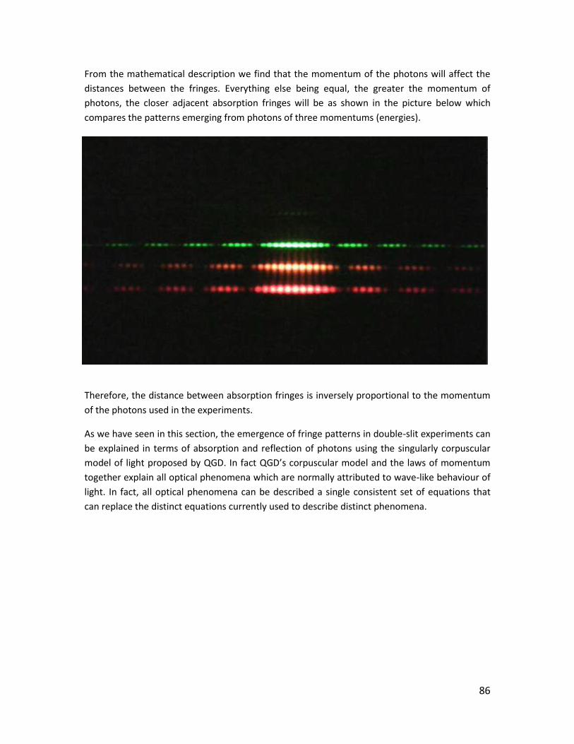
86
From the mathematical description we find that the momentum of the photons will affect the
distances between the fringes. Everything else being equal, the greater the momentum of
photons, the closer adjacent absorption fringes will be as shown in the picture below which
compares the patterns emerging from photons of three momentums (energies).
Therefore, the distance between absorption fringes is inversely proportional to the momentum
of the photons used in the experiments.
As we have seen in this section, the emergence of fringe patterns in double-slit experiments can
be explained in terms of absorption and reflection of photons using the singularly corpuscular
model of light proposed by QGD. In fact QGD’s corpuscular model and the laws of momentum
together explain all optical phenomena which are normally attributed to wave-like behaviour of
light. In fact, all optical phenomena can be described a single consistent set of equations that
can replace the distinct equations currently used to describe distinct phenomena.

87
QGD Interpretations of Redshift Effects
A consequence of QGD’s axiom of discreteness of space implies that all electromagnetic
radiations are singularly corpuscular emissions and, as we have seen earlier in this section, the
wave-like behaviour of light emerges from interactions between photons and structures which
fundamentally are all discrete. Because of its corpuscular nature, the properties of a photon do
not change between its emission and detection (unless it interacts with matter along its
trajectory), hence the apparent redshift of the emission spectrum occurs either at the source of
emission (intrinsic redshift) or during its detection. The redshift therefore does not result from a
shift in the momenta of photons along their trajectories between emission and detection but, as
explained below, is simply a measurement of the difference between the momenta of photons
of the emission spectrum of electrons of a given element from two distinct sources, one the
observed source and the other the reference source.
Intrinsic Redshift
We have seen that changes in momentum of electrons obey the law
[1]e e
P m
which imposes that only photons such that
[2]e
P m can be absorbed or emitted.
Equation [1] governs not only changes in momentum that are induced by the absorption of
emission of a photon, but also momentum changes resulting from variations in gravity or the
electromagnetic field effect, the latter resulting from a variation in the preonic density. Hence
taking gravity and the electromagnetic effect into account we get:
[3]e e
P P G m where G is the variation in gravity and is the variation
in the magnitude of electromagnetic interaction of the atomic electron is subjected to.
Since the law of momentum [1] must be obeyed then from equation [3] we see that an increase
in gravity or the preonic density or both proportionally decreases the permitted momentum of
photons an electron can absorb or emit. Conversely, if gravity and/or the preonic density
decrease(s) then the permitted momentum for photons to be absorbed or emitted increases
proportionally since
[4]e
P m G .
An increase in gravity will therefore reduce the momentum necessary for photons to be
absorbed or emitted by the source and as a consequence, the absorption and emission
spectrum of the source atoms will be redshifted.
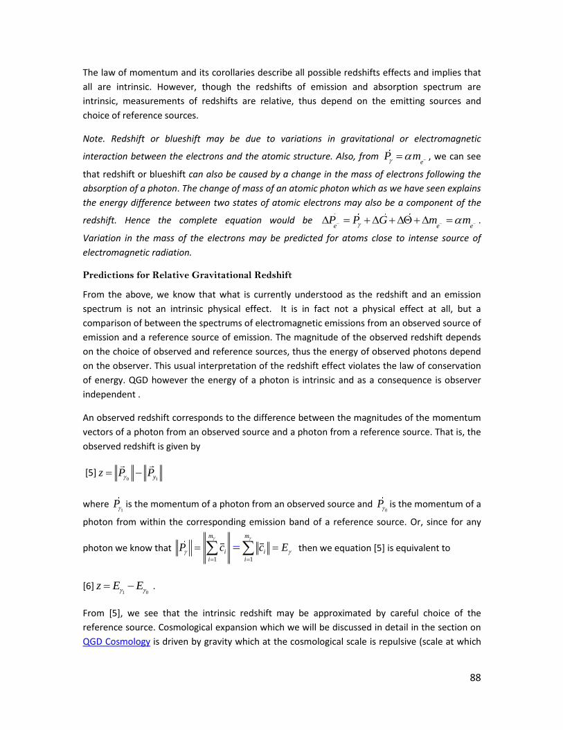
88
The law of momentum and its corollaries describe all possible redshifts effects and implies that
all are intrinsic. However, though the redshifts of emission and absorption spectrum are
intrinsic, measurements of redshifts are relative, thus depend on the emitting sources and
choice of reference sources.
Note. Redshift or blueshift may be due to variations in gravitational or electromagnetic
interaction between the electrons and the atomic structure. Also, from e
P m , we can see
that redshift or blueshift can also be caused by a change in the mass of electrons following the
absorption of a photon. The change of mass of an atomic photon which as we have seen explains
the energy difference between two states of atomic electrons may also be a component of the
redshift. Hence the complete equation would be e e e
P P G m m .
Variation in the mass of the electrons may be predicted for atoms close to intense source of
electromagnetic radiation.
Predictions for Relative Gravitational Redshift
From the above, we know that what is currently understood as the redshift and an emission
spectrum is not an intrinsic physical effect. It is in fact not a physical effect at all, but a
comparison of between the spectrums of electromagnetic emissions from an observed source of
emission and a reference source of emission. The magnitude of the observed redshift depends
on the choice of observed and reference sources, thus the energy of observed photons depend
on the observer. This usual interpretation of the redshift effect violates the law of conservation
of energy. QGD however the energy of a photon is intrinsic and as a consequence is observer
independent .
An observed redshift corresponds to the difference between the magnitudes of the momentum
vectors of a photon from an observed source and a photon from a reference source. That is, the
observed redshift is given by
[5]0 1yz P P
where 1
P is the momentum of a photon from an observed source and 0
P is the momentum of a
photon from within the corresponding emission band of a reference source. Or, since for any
photon we know that 1 1
m m
i i
i i
P c c E
then we equation [5] is equivalent to
[6]1 0
z E E .
From [5], we see that the intrinsic redshift may be approximated by careful choice of the
reference source. Cosmological expansion which we will be discussed in detail in the section on
QGD Cosmology is driven by gravity which at the cosmological scale is repulsive (scale at which
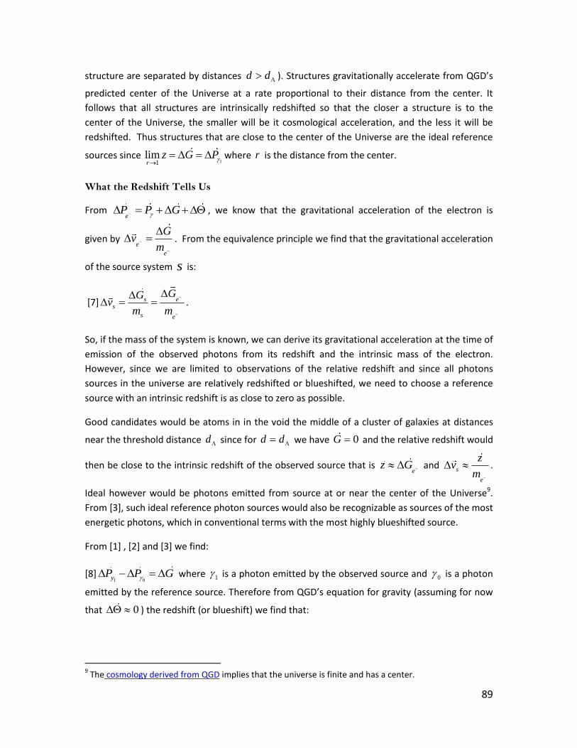
89
structure are separated by distances d d ). Structures gravitationally accelerate from QGD’s
predicted center of the Universe at a rate proportional to their distance from the center. It
follows that all structures are intrinsically redshifted so that the closer a structure is to the
center of the Universe, the smaller will be it cosmological acceleration, and the less it will be
redshifted. Thus structures that are close to the center of the Universe are the ideal reference
sources since 11
limr
z G P
where r is the distance from the center.
What the Redshift Tells Us
From e
P P G , we know that the gravitational acceleration of the electron is
given by e
e
Gv
m
. From the equivalence principle we find that the gravitational acceleration
of the source system s is:
[7] s es
s e
GGv
m m
.
So, if the mass of the system is known, we can derive its gravitational acceleration at the time of
emission of the observed photons from its redshift and the intrinsic mass of the electron.
However, since we are limited to observations of the relative redshift and since all photons
sources in the universe are relatively redshifted or blueshifted, we need to choose a reference
source with an intrinsic redshift is as close to zero as possible.
Good candidates would be atoms in in the void the middle of a cluster of galaxies at distances
near the threshold distance d since for d d we have 0G and the relative redshift would
then be close to the intrinsic redshift of the observed source that is e
z G and s
e
zv
m
.
Ideal however would be photons emitted from source at or near the center of the Universe9.
From [3], such ideal reference photon sources would also be recognizable as sources of the most
energetic photons, which in conventional terms with the most highly blueshifted source.
From [1] , [2] and [3] we find:
[8]1 0yP P G where 1 is a photon emitted by the observed source and 0 is a photon
emitted by the reference source. Therefore from QGD’s equation for gravity (assuming for now
that 0 ) the redshift (or blueshift) we find that:
9 The cosmology derived from QGD implies that the universe is finite and has a center.

90
for d d , d being the threshold distance below with gravity is attractive, objects
moving away from us will be blueshifted while objects moving towards us will be redshifted and,
for d d , lights emitted by objects moving away from us will be redshifted while light
emitted by objects moving towards us will be blueshifted.
The graphics below compare the distinct predictions of QGD and standard cosmology.
The arrows indicate the direction of motion of the observed object
Noteworthy is that, contrary to standard cosmology, the gravitational redshift and blueshift
mechanisms which QGD describe do not violate the laws of conservation of energy. Also, the
redshift equation takes into account what is referred to as dark energy (which is caused by
gravity becoming repulsive for d d ); predicting different behaviour of the redshifts and
blueshifts for d d and d d .
QGD Cosmology
-z
+z
-z
+z
Standard Cosmology
-z
+z
-z
+z

91
From [3] and [5], we
understand that the greater
z G , thus the effect will
be most noticeable when a
star moves close to a high
density object such as a black
hole. The redshift of a the
spectrum of a star near a black
hole has been recently
observed10 and though it is
taken as confirmation of the
gravitational redshift
predicted by general relativity,
the observation is also
consistent with the predictions
of QGD as shown in the figure
below where the light from a
star orbiting a black hole will
redshifted relative to a
reference source orbiting at a
larger distance.
It is interesting to note that all redshift effects are described by a single equation (equation [5]))
while several different mechanisms are required for the Doppler cosmological redshift, the
redshift and the gravitational redshift, but most importantly, the relation expressed in [3] relates
the dark energy effect (repulsive gravity for d d ), but as we will see in the section on QGD
cosmology, it also links dark matter and the electromagnetic interactions between particles
(since _preonic density , hence proportional to the density of the dark matter halo).
10
https://arxiv.org/abs/1807.09409v1
reference source
observed source
The length of the green arrows represents the magnitude of the gravitational interaction between a black hole and a reference star orbiting it (top) compared to an observed star in the same system (bottom).

92
Mapping the Universe
Though the mechanism of the redshift effect is the same at all scales, its interpretations differs
depending on the scale of the scope of observations. An increase of the gravitational
acceleration affecting an observed source will always cause a shift in the emission spectrum of
the atom, but from QGD’s equation of gravity we know that, as with Newtonian gravity, the
gravitational interaction decreases as a function of distance but it is the opposite beyond the
threshold distance d where gravity increases with distance.
When observed and reference sources are separated by distances smaller than the threshold
distance d , a reduction in the magnitude of the gravitational interaction an observed object is
submitted to will, according to equation [5], result in a blueshift of the emission spectrum
compared to that of its previous position while an increase in the gravitational interaction will
produce a redshift. This has been observed recently when the light from a star approaching
Sagittarius A* was redshifted. However, the opposite will be observed when observed sources
are at distances greater than the threshold distance.
As a consequence, mapping the observable Universe requires that we apply scale appropriate
interpretations of the redshift effect to observations. For electromagnetic signals, taking into
account the distance of the source (using luminosity and scattering of photons) allows us to
establish the state the Universe at the moment of their emissions.
For gravitational signals, assuming that gravity is instantaneous, all signals describe the changes
of state the objects as they occur which implies that all simultaneous gravitational signals
correspond to simultaneous events. Therefore, gravitational signals may help us create a map of
the universe in “real time.”
Different cosmologies provide different interpretations of observational data and draw different
maps of the Universe. As we will see in the section on QGD cosmology, QGD predicts that the
universe is finite therefore it must have a center and an edge. Interpreted by QGD, the
measurements of redshifts draw a map very different from that obtained by applying standard
cosmology. But though different QGD’s map is not only consistent with observations of stellar
objects but consistent with the laws of physics that describe reality at all scales from the most
fundamental to the cosmological. QGD’s description of the Universe is consistent with the law of
gravity and the laws of momentum and does not require spatial dimensions beyond the three
that we know, nor does it need any ad hoc particles or mechanisms to explain such things as the
dark matter or dark energy effects. QGD describes reality using the smallest possible number of
initial assumptions; the minimal axiom set necessary to describe dynamic systems.
We will continue this discussion in the QGD Cosmology section.
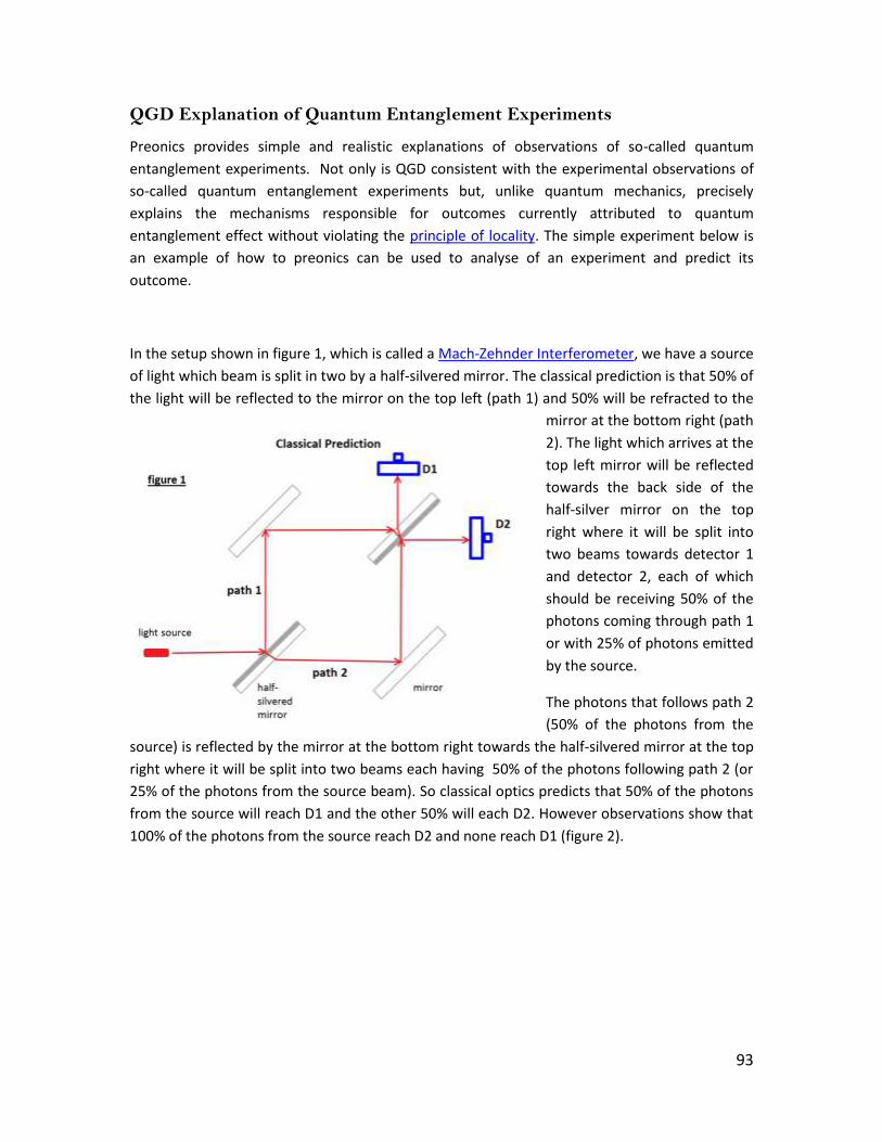
93
QGD Explanation of Quantum Entanglement Experiments
Preonics provides simple and realistic explanations of observations of so-called quantum
entanglement experiments. Not only is QGD consistent with the experimental observations of
so-called quantum entanglement experiments but, unlike quantum mechanics, precisely
explains the mechanisms responsible for outcomes currently attributed to quantum
entanglement effect without violating the principle of locality. The simple experiment below is
an example of how to preonics can be used to analyse of an experiment and predict its
outcome.
In the setup shown in figure 1, which is called a Mach-Zehnder Interferometer, we have a source
of light which beam is split in two by a half-silvered mirror. The classical prediction is that 50% of
the light will be reflected to the mirror on the top left (path 1) and 50% will be refracted to the
mirror at the bottom right (path
2). The light which arrives at the
top left mirror will be reflected
towards the back side of the
half-silver mirror on the top
right where it will be split into
two beams towards detector 1
and detector 2, each of which
should be receiving 50% of the
photons coming through path 1
or with 25% of photons emitted
by the source.
The photons that follows path 2
(50% of the photons from the
source) is reflected by the mirror at the bottom right towards the half-silvered mirror at the top
right where it will be split into two beams each having 50% of the photons following path 2 (or
25% of the photons from the source beam). So classical optics predicts that 50% of the photons
from the source will reach D1 and the other 50% will each D2. However observations show that
100% of the photons from the source reach D2 and none reach D1 (figure 2).

94
The explanation provided
by quantum mechanics,
which is similar to that
given for the results of
double-slit experiments,
proposes that the wave
function of each individual
photon travels both paths
and engages in
interference at the half-
silvered mirror on the top
right and that they
interfere destructively at
D1 and constructively at D2
(a detailed explanation can
be found here).
Applying the QGD optics to analyse the setup, we find a different and much simpler explanation.
At the point of intersection
in the top right half-silvered
mirror (yellow circle in
Figure 3),
1 1 2 2cos cos
eP P m
so that the photons 2 are
reflected to D2 as per the
mechanism of reflection we
described above.
Now consider the setup
shown in figure 5.
Observations show that in
this setup 50% of the photons
reach D3, 25% of the photons
that will reach each of D1 and
D2 detectors.
According to quantum
mechanics, the photons
moving along path 2 that
reach D1 can only do so if the
photons moving along path 1
D2
D1figure 3
path 1
path 2
D2
half-silvered mirror
mirror
light source
D1
D3
Experimental Observation 2
path 2
path 1
figure 4

95
are deflected towards D3. This raises the question: How the photons that reach D1 know that
the photons of path 1 were deflected towards D3?
The quantum mechanical explanation is that the photons from path 1 and path 2 are entangled,
a phenomenon known as quantum entanglement, by which a change done to photons on path
1, by a measurement for example, instantly affects the photons moving on path 2. And,
according to quantum mechanics, it does so instantly and independently of the distance that
separate the entangled photons. This explanation of course violates locality, but this violation is
essential to quantum mechanics if it is to describe the observations of experiments such as the
ones we described above. The observations in turn, as interpreted by quantum mechanics,
support the existence of
quantum entanglement and
non-locality.
Again QGD provides a much
simpler and realistic
interpretation of observations.
That is: Since no photons from
path 1 reach the point of
interaction of top right mirror,
then then 1 1cos 0P and
1 1 2 2cos cos
eP P m .
That the mirror is transparent
to photons of momenta2
P ,
means that 2 e
P m so the photons 2 from path 2 can be absorbed by the outer electrons
and allowed to move towards D1 as per the refraction mechanism we described earlier.
The example above illustrates that the outcome of so-called quantum entanglement can easily
be explained classically from a complete physical description of the experiments. Complete
physical descriptions of all other experiments supporting quantum entanglement will also
provide the basis for classical explanations.

96
Distances and Intrinsic Luminosities of 1a Supernovas
First we need to choose a reference type 1a supernova with the largest blueshift and measure
its distance refd from it parallaxes so as to eliminate physical assumptions (such measurement
will be possible using the data from the GAIA or similar mission). Based on QGD’s explanation of
the redshift effect, we understand that the electromagnetic emission from such a supernova is
its intrinsic spectrum.
Once the distance is known, we can calculate its intrinsic luminosity using the formula 2*4
refrefL Flux d where theref
Flux is the number of photonsref of a given momentum
or energy (since these properties are numerically equal for photons).
In order to measure the distance of another type 1a supernova (SN) we must determine its
redshift. The redshift is used here to determine the position on the redshifted spectrum of the
supernova where we will find photons SN that have the same intrinsic energy as the reference
photons ref .
SNFlux is the number of SN photons.
If the luminosities of type 1a supernovas are comparable (the accepted assumption), that is: if
ref SNL L , then 2*4SNref SNL Flux d and
4SN
ref
SN
Ld
Flux .
Derivation of the Intrinsic Velocity of Earth from Type 1a Supernovas
Also, using QGD’s description of the redshift effect, we can calculate av , the intrinsic speed of
the Earth (or that of any detector in space), using three non-coplanar reference supernovas.
Since SN SN SNi i i
a ac v m P , then SN SNi i
SNi
aa
Pv c
m
and
1 2 3SN SN SNa a a av v v v .
Conclusion
If QGD’s explanation of the redshift effect is confirmed, then it will be possible to measure the
intrinsic speed not only of the Earth (its absolute speed) but of other observable objects and
from it, derive the values of other intrinsic properties such as momentum and mass.

97
QGD States of Atomic Electrons
In this section, we show how the energy states of atomic electrons follow naturally from the
laws of momentum.
For simplicity, we will describe of the energy states of the electron of hydrogen atom system but
the same principles apply to complex atomic systems.
A ground state of an atomic electron is the state of equilibrium between the extrinsic forces
acting on it. For hydrogen, which consists only of a proton and an electron, the extrinsic forces
are the forces between them that act on the electron. For more complex elements, the extrinsic
forces are produced by the interactions of a given electron, the other electrons and the
components of the nucleus. And as we will see, each of the electrons has a ground state that is
dependent on the ground states of all the other electrons.
At ground state 1
0e
n
i
i
F
where the i indexes the an extrinsic forces acting on e . These
forces are either gravitational (which QGD’s equation for gravitational interactions predicts must
be over a hundred orders of magnitude greater at the atomic scale than at cosmic scale) or
electromagnetic which is actually the resulting effect of the interactions between charges
particles and the free preons
which as we have seen earlier for the magnetic field.
The third law of momentum dictates that permitted changes in momentum of any particle or
structure a is proportional to its mass. That is: a aP m or for an electron e e
P m .
where N .
Let 0 denote the ground state of the electron of a hydrogen atom and 0 be a photon such
that 0
0e
P m
. The electron 0
e
can absorb 0 since it imparts a change in momentum that
respects the third law; that is: 0 e e
P P m where 1 . After absorption of the
photon, the electron’s momentum has changed from state 0 to state 1 . The momentum
vector, mass and energy of the electron in 1 states are respectively 0
1 0e e
P P P
,
01 0
e em m m
and 0 0
1 0 0e e e
E E E m m c
.
The change in the momentum vector also changes the distance between the electron and the
proton so that 1
10 11
en
i
i
F F P
. So if there is no other force acting on 1
e
, it will be pushed
back to its 0 state and it can be on this state of equilibrium by respecting by emitting a photon
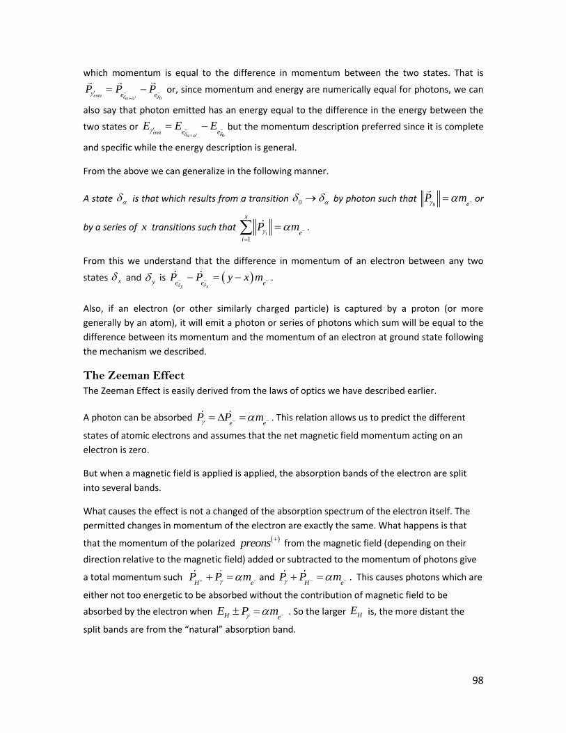
98
which momentum is equal to the difference in momentum between the two states. That is
0emit e e
P P P
or, since momentum and energy are numerically equal for photons, we can
also say that photon emitted has an energy equal to the difference in the energy between the
two states or 0
emit e eE E E
but the momentum description preferred since it is complete
and specific while the energy description is general.
From the above we can generalize in the following manner.
A state is that which results from a transition 0 by photon such that 0 e
P m or
by a series of x transitions such that 1
i
x
ei
P m
.
From this we understand that the difference in momentum of an electron between any two
states x and y is
y xe e e
P P y x m .
Also, if an electron (or other similarly charged particle) is captured by a proton (or more
generally by an atom), it will emit a photon or series of photons which sum will be equal to the
difference between its momentum and the momentum of an electron at ground state following
the mechanism we described.
The Zeeman Effect
The Zeeman Effect is easily derived from the laws of optics we have described earlier.
A photon can be absorbed e e
P P m . This relation allows us to predict the different
states of atomic electrons and assumes that the net magnetic field momentum acting on an
electron is zero.
But when a magnetic field is applied is applied, the absorption bands of the electron are split
into several bands.
What causes the effect is not a changed of the absorption spectrum of the electron itself. The
permitted changes in momentum of the electron are exactly the same. What happens is that
that the momentum of the polarized preons
from the magnetic field (depending on their
direction relative to the magnetic field) added or subtracted to the momentum of photons give
a total momentum such H e
P P m and H e
P P m . This causes photons which are
either not too energetic to be absorbed without the contribution of magnetic field to be
absorbed by the electron when H e
E P m . So the larger HE is, the more distant the
split bands are from the “natural” absorption band.

99
For H e
E P m , instead of the absorption band for , there will be two absorption bands
corresponding to photons and with momentum HP P P and
HP P P . For
2H eE P m There will be four absorption bands 2H e
E P m corresponding to
1 1H eP P P m ,
22H e
P P P m ,2 1H e
P P P m , 2
2H eP P P m .
In special cases when H e
E m , the split of bands will be symmetric to the natural
absorption band. When H e
E m
Number of bands _ 2nbr bands for H e
E m and _ 2 1nbr bands for
H eE m .
H
e
E Pm
H
e
E Pm
The momentum of 1i i i ie e e e
P P m P P
and 1i ie e
m m m
so that the for a photon
1i to be absorbed by an electron in the 1i state , 1i iie
P m m .
States of Muonic Hydrogen
In the previous section we have shown that the difference between to states is dependent upon
the mass of the electron. This implies that in muonic hydrogen, in which the electron has been
replaced by a muon, which particle as greater mass, then the momentum difference between
two states of the muon will be greater than the difference between two equivalent states of the
electron of ordinary hydrogen.
So to return to ground state from a higher state, since uP ym and e e
P ym during
the 0y transition the muon of muonic hydrogen will emit a photon with higher
momentum (and energy) than that of photon emitted by the electron of ordinary hydrogen. This
is consistent with the measurements of recent experiments11 which quantum mechanical
interpretation led to the proton size problem.
Determination of the Proton Size
Quantum mechanics correctly predicts that the transition energy of an electron between states
is the difference between the energies specific to each state. The momentum of the photon
11
Muonic hydrogen and the proton radius puzzle, R. Pohl, R. Gilman, G. A. Miller, K. Pachucki http://arxiv.org/abs/1301.0905

100
emitted during the transition between two given states should not be the same for the muonic
hydrogen and ordinary hydrogen as shown by recent experiments show that this is not the case.
We have shown that the momentum gaps between two permitted states, known as Lamb shifts,
is dependent on the mass of the particle. Therefore, when taking this into account, there will be
no discrepancy between the size of the proton derived from hydrogen experiments from that
derived from muonic hydrogen or any other experiment.
Radius of a Proton
If the masses of the proton and electron in fundamental units are known, then:
1. Resolve the equation for the electromagnetic effect to obtain the distance between the
region occupied by the electron and that which is occupied by the proton and
2. resolve the gravitational interaction equation to find the distance between the electron
and the centre of gravity of the proton.
3. The difference between the two will give the radius of the proton.
The QGD description of the electromagnetic effect will be derived and discussed in a dedicated
section.
The Photoelectric Effect
Consider a state x of an atomic electron interacting with a photon where x
eP m
. If
1 1
e
i
x
n
ei
P F
, then the electron will become unbounded and the momentum of the
unbound electron will be 1 xx
e eP P P
. The above 1x x transition is the
photoelectric effect.
Conclusion
We have shown that the mechanisms of atomic electron transition as derived from QGD’s axiom
set not only describes observations but provides a fundamentally based explanation. Also, the
model is consistent with muon states transitions of muonic hydrogen.
101
Heat, Temperature and Entropy
Using the concepts we have introduced so far, we will now derive the properties of heat,
temperature and entropy.
Given a system S having n unbound particles, the heat of the system is equal to1
n
i
i
P
, where
iP is the magnitude of the momentum vector of the nti particle and its temperature is 1
n
i
i
S
P
Vol
.where SVol is the volume of the system measured in preons
, the fundamental and discrete
particle which forms and dimensionalizes quantum-geometrical space. The total energy of the
system being equal to1
n
i
i
m c
, it follows that if we define entropy in the classical sense, then
the entropy of S is1 1
n n
i i
i i
m c P
.
Application to Exothermic Reactions within a System
The QGD definitions can be used to describe the changes in heat and temperature resulting
from chemical or nuclear reactions. The particles involved are different, as are the reaction
mechanisms, and the reactions occur at different scales, but both result in changes in the
structure and number of bound particles.
Consider 1 2S S where 1S is a dynamic system containing 1n unbound particles (or structures)
some of which reacting with each other, and 2S the resulting system containing 2n unbound
particles, if 2 1n n then1 2
1 1
'n n
i i
i i
P P
and the change in heat of the system
2 1
1 1
'n n
i i
i i
PH P
is positive.
For example, let say the system contains only a particle e and a particle e
which annihilate to
give n photons ( ), then 1
i
n
ee e ei
m c v mH v m
. Here, the difference in heat
depends on the speed of interacting electrons and is at the lowest when electrons achieve the
speed of light; in which case 0H .Note that from the QGD model, when electrons achieve c
, internal motion stops, so that component preons
move in parallel trajectories.
Also, QGD predicts that electrons accelerated to c become indistinguishable from photons and
become electrically neutral. The electrical charge of a particle is caused by internal motion of its

102
component preon
which interact with the preonic field (the free
preons
populating
quantum-geometrical space). Since all internal motion stop at speed c , the electron moving at
that speed must lose their electric charge.
Also worth nothing is that 1
i
n
eei
m m m
which implies that1 2S SE E ,that is; mass and
energy are conserved. This holds for all closed systems. So though it is believed that a nuclear
reaction results in the conversion of mass into energy, according to QGD, it results in the freeing
of bound particles which carry with them momentum, hence increase the heat of the system.
Aside from the reaction mechanism, the only difference between exothermic chemical and
nuclear reactions is in the type of particles that become free. For chemical reactions these
particles are molecules, atoms and photons and for nuclear reactions, nuclei and other
subatomic particles.
Implication for Cosmology
In the initial state of the Universe, QGD theorizes that all preons
were free. That means that
the energy of the Universe was equal to its heat. So if that its entropy was equal to zero. That is:
1
0n
U i
i
m c P
, where Um is the masse of the Universe in preons
and since all
preons
are free Um n . It follows that the temperature of Universe in its initial state was 0
U U
U
m cT
Vol .
Though the Universe as evolved, its total energy remains Um c , but as particles and structures
are formed its heat decreases resulting in an increase in entropy according. In formal terms we
have 1
0n
U i
i
m c P
).
In the upcoming section “Cosmology Derived from Quantum-Geometry Dynamics” we will show
that in its initial state the temperature of the universe was 0
cT
k where c the kinetic energy
of the preon
and k the proportionality constant between the n-gravity and p-gravity.
103
QGD Equations Applicability
First, since all fundamental properties are associated with preons
and
preons
, and
because the properties of neither can be directly measured, it is impossible to experimentally
determine their values, therefore we cannot convert QGD units into conventional measurable
units. However, assuming that the relations between physical quantities described by QGD are
valid, we may use the absolute values of physical properties of mass, momentum, velocity
expressed in conventional units and the constants c and k 12.
Assigning Value to k
QGD’s equation for gravitational interactions is 2
;2
a b
d dG a b m m k
where am and
bm are the absolute masses of objects of a and b . From the question we can predict that
; 0G a b when 2
2
d dk ( d is the threshold distance beyond which gravity becomes
negative13) . Recent observations14 suggest that 10d Mpc in which case 344.5*10k when
using the meter as unit of distance in the gravity equation.
Assigning Value to c
As we have discussed earlier, for calculations we must substitute the intrinsic velocity of light by
it’s the absolute velocity of light as given by two way measurement experiments.
Measurement of Absolute Masses
We can use the equivalence principle as derived by QGD and the equation relating gravitational
deflection of light to the mass of the deflecting object to determine the absolute mass of an
object.
Let us take the sun for example.
The absolute mass is obtained as follow.
1. Measure the angle of deflection of light from the sun. 2. Use the equation describing the relation between mass of the light deflecting objet and
resolve it for the mass of the sun m .
12 We must however keep in mind that properties such as mass, energy, momentum, velocity, charge,
etc., take on different meanings in QGD since it considers intrinsic and absolute.
13 for d d gravity becomes negative and is, as we explained, is responsible for the effect we call dark
energy 14
Dark energy and key physical parameters of clusters of galaxies http://arxiv.org/abs/1206.1433

104
Measurement of Absolute Velocity
All direct measurements of velocity are relative to a chosen frame of reference. However, it is
possible to measure the absolute velocity of the Earth using the redshift effect and once this is
known, it becomes possible to deduce the absolute or intrinsic velocities of any object.
Continuing with our previous example.
3. Once we know the absolute mass of the sun, we can use QGD’s equation for gravity and the absolute motion of the Sun and Earth to calculate the absolute mass of the Earth.
4. The absolute velocity of the Earth and be obtained using the redshift effect described here. Once the absolute velocity of the Earth is known, we can deduce the absolute velocities of other objects from their velocity relative to the Earth.
Rest Mass and Relativistic Mass
Unless an object absorbs particle (which it does only when non-gravitational forces are applied
to a body) the mass of an object does not change with speed.
The mass remains equal to the number of preons
it contains. What changes under the
influence of gravity is the net orientation of their components preons
, what we call its
momentum given by the equation 1
am
a i
i
P c
. The magnitude of aP increases in towards b
when ; 0G a b and increases away from b when ; 0G a b but as we explained it mass
am or its energy 1
am
i
i
c
remain constant.
A body is at rest if its momentum is equal to zero. That is1
0am
i
i
c
.
The relation between mass and energy expressed by 1
am
a i a
i
E c m c
is a proportionality
relation. Here again, the relativistic and QGD mass are one and the same.
Assigning Value to c
Since
;
sinG a
P
so that
2
2sin
a
d dm m k
m c
then
2
2
sin
a
d dm k
c
.
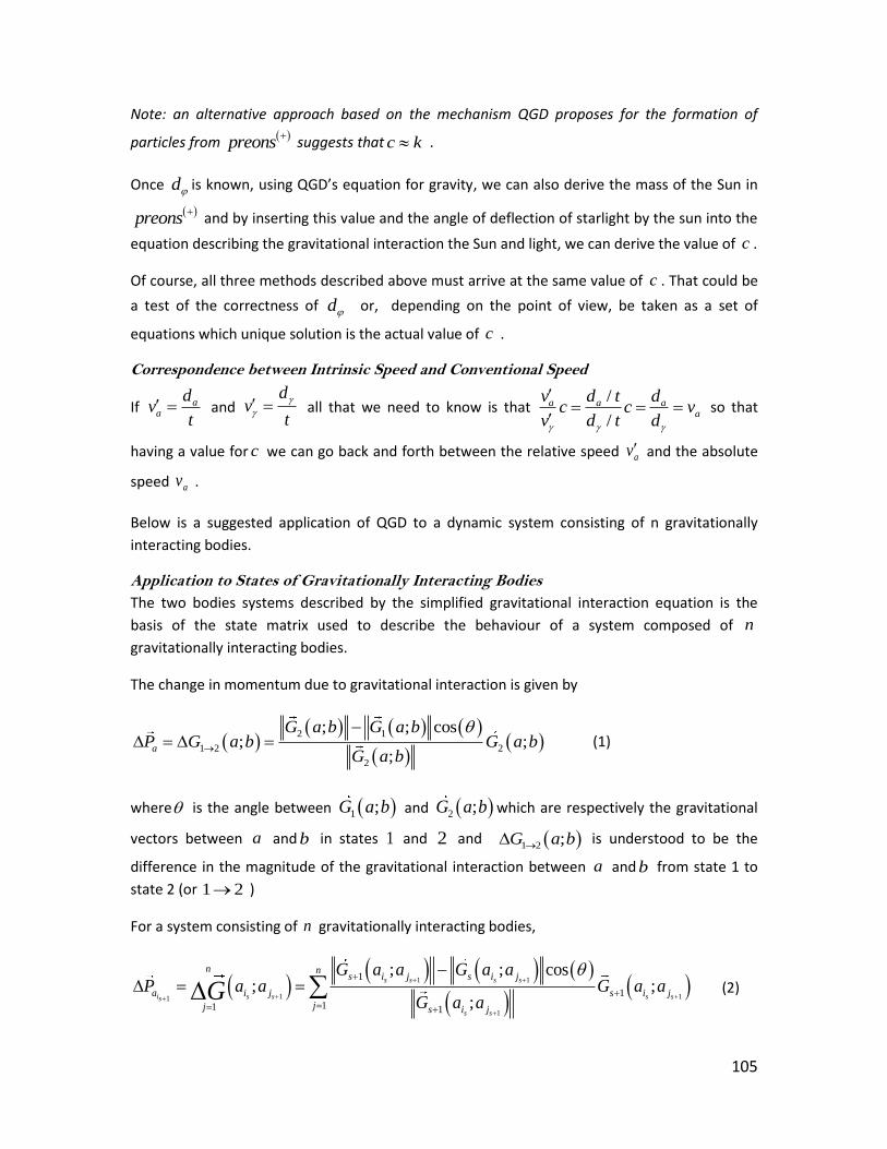
105
Note: an alternative approach based on the mechanism QGD proposes for the formation of
particles from preons
suggests that c k .
Once d is known, using QGD’s equation for gravity, we can also derive the mass of the Sun in
preons
and by inserting this value and the angle of deflection of starlight by the sun into the
equation describing the gravitational interaction the Sun and light, we can derive the value of c .
Of course, all three methods described above must arrive at the same value of c . That could be
a test of the correctness of d or, depending on the point of view, be taken as a set of
equations which unique solution is the actual value of c .
Correspondence between Intrinsic Speed and Conventional Speed
If aa
dv
t and
dv
t
all that we need to know is that
/
/
a a aa
v d t dc c v
v d t d
so that
having a value for c we can go back and forth between the relative speed av and the absolute
speed av .
Below is a suggested application of QGD to a dynamic system consisting of n gravitationally
interacting bodies.
Application to States of Gravitationally Interacting Bodies
The two bodies systems described by the simplified gravitational interaction equation is the
basis of the state matrix used to describe the behaviour of a system composed of n
gravitationally interacting bodies.
The change in momentum due to gravitational interaction is given by
2 1
1 2 2
2
; ; cos; ;
;a
G a b G a bP G a b G a b
G a b
(1)
where is the angle between 1 ;G a b and 2 ;G a b which are respectively the gravitational
vectors between a and b in states 1 and 2 and 1 2 ;G a b is understood to be the
difference in the magnitude of the gravitational interaction between a and b from state 1 to
state 2 (or 1 2 )
For a system consisting of n gravitationally interacting bodies,
1 1
1 11
1
1
1
11 1
; ; cos; ;
;
s s s s
i s s s ss
s s
n ns i j s i j
a i j s i j
jj s i j
G a a G a aP a a G a a
G a aG
(2)
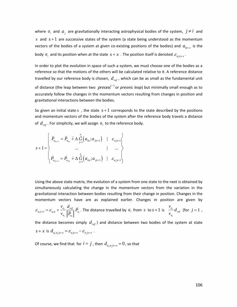
106
where ia and ja are gravitationally interacting astrophysical bodies of the system, j i and
s and 1s are successive states of the system (a state being understood as the momentum
vectors of the bodies of a system at given co-existing positions of the bodies) and |i s xa
is the
body ia and its position when at the state s x . The position itself is denoted |ia s x
.
In order to plot the evolution in space of such a system, we must choose one of the bodies as a
reference so that the motions of the others will be calculated relative to it. A reference distance
travelled by our reference body is chosen, refd , which can be as small as the fundamental unit
of distance (the leap between two preons
or preonic leap) but minimally small enough as to
accurately follow the changes in the momentum vectors resulting from changes in position and
gravitational interactions between the bodies.
So given an initial state s , the state 1s corresponds to the state described by the positions
and momentum vectors of the bodies of the system after the reference body travels a distance
of refd . For simplicity, we will assign 1a to the reference body.
1| 1 1| 1
| 1 |
1| | 1 | 11
| | 1 | 11
; |
1 ... | ...
; |
s s
n s n s n
n
a a s j s a sj
n
a a n s j s a sj
P P G a a
s
P P G a a
Using the above state matrix, the evolution of a system from one state to the next is obtained by
simultaneously calculating the change in the momentum vectors from the variation in the
gravitational interaction between bodies resulting from their change in position. Changes in the
momentum vectors have are as explained earlier. Changes in position are given by
1
| 1 |i
i i i
i
a ref
a s a s a
a a
v dP
v P . The distance travelled by ia from s to 1s is
1
ia
ref
a
vd
v (for 1j ,
the distance becomes simply refd ) and distance between two bodies of the system at state
s x is ; | | |i j i ja a s x a s x a s xd .
Of course, we find that for i j , then ; | 0i ja a s xd , so that

107
1 | 1 | 1 | 1 | 1 | |
2 2; | 1 ; | 1 ; | ; |
; ; ;
2 2
0
i i i j i i i i
s i s j s i s i s i s i s
a a s a a s a a s a a s
a a a a
a a a a
G a a G a a G a a
d d d dm m k m m k
m m k m m k
,
the variation in the gravitational interaction between a body with itself is equal to zero, which
implies that its momentum vector will remain unchanged unless 1n and | | 11
; 0n
n s j sjG a a
. This is the QGD explanation of the first law of motion.
Note also that for an object ja freefalling towards an object ia , 0 so equation (2)
becomes
1 1
1 11
1
1
1
1 1
; ;; ;
;
s s s s
i s s s ss
s s
ns i j s i j
a i j s i j
j s i j
G a a G a aP a a G a a
G a aG
and
1 1 1
1 1 1 1 1 1
1 1
1
1 1
1 1
; ;; ; ; ;
;
s s s s
s s s s s s s s
s s
ns i j s i j
i j s i j s i j s i j
j s i j
G a a G a aa a G a a G a a G a a
G a aG
Alternative Measurements of Earth’s Intrinsic Speed
We have seen how the intrinsic speed of the Earth can be measured from type 1a supernovas.
Below is an alternative experiment.
If QGD is correct, then it is possible to measure the intrinsic speed15 of the Earth and other
cosmic objects.
All that is needed to do is to measure the one way distance travelled by light in three mutually
perpendicular directions.
Each distance would be measured by a clock each cycle of it being made to correspond to a
reference distance which is the distance that light. Since the distance travelled by the Earth is
cancelled out in all two way distance measurements of light, then cref
dd
n where cd is the
two way distance and n the number of clocks cycles counted between emission and return of
the light signal.
So1 1 refd n d ,
2 2 refd n d and3 3 refd n d then
15
Intrinsic speed may be thought as absolute speed by opposition to relative speed.

108
1
1
c
c
d dv c
d
, 2
1
c
c
d dv c
d
, 3
3
c
c
d dv c
d
and
1 2 3
2 2 2v v v v
Measurements of the Intrinsic Speed of a Distant Light Source
Once the intrinsic speed and direction of the Earth is known, the effect of its effect on the
redshift of light received from a distant source can be factored out. Then, using the QGD’s
description of the redshift effect, we can calculate the intrinsic speed of the distant light source
at the time the light was emitted.
However, measurements of variation in gravitational interactions with distant objects would
provide their current instantaneous position and speed.
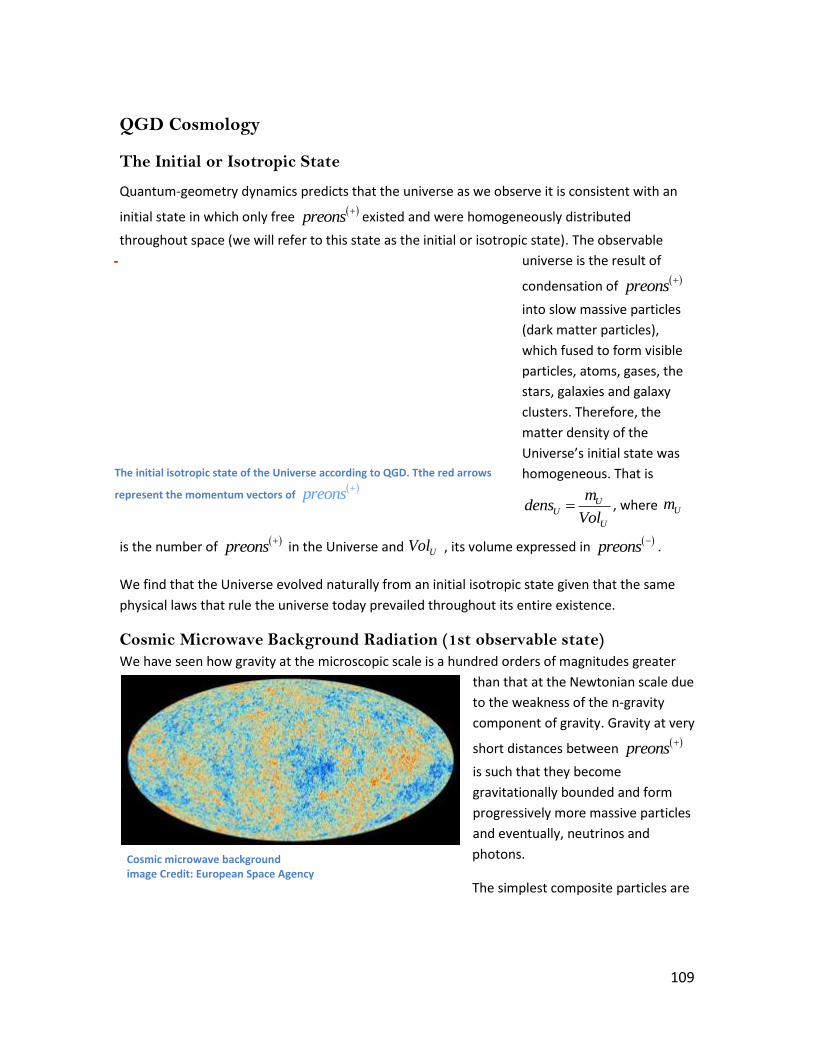
109
QGD Cosmology
The Initial or Isotropic State
Quantum-geometry dynamics predicts that the universe as we observe it is consistent with an
initial state in which only free preons
existed and were homogeneously distributed
throughout space (we will refer to this state as the initial or isotropic state). The observable
universe is the result of
condensation of preons
into slow massive particles
(dark matter particles),
which fused to form visible
particles, atoms, gases, the
stars, galaxies and galaxy
clusters. Therefore, the
matter density of the
Universe’s initial state was
homogeneous. That is
UU
U
mdens
Vol , where Um
is the number of preons
in the Universe and UVol , its volume expressed in
preons
.
We find that the Universe evolved naturally from an initial isotropic state given that the same
physical laws that rule the universe today prevailed throughout its entire existence.
Cosmic Microwave Background Radiation (1st observable state)
We have seen how gravity at the microscopic scale is a hundred orders of magnitudes greater
than that at the Newtonian scale due
to the weakness of the n-gravity
component of gravity. Gravity at very
short distances between preons
is such that they become
gravitationally bounded and form
progressively more massive particles
and eventually, neutrinos and
photons.
The simplest composite particles are
Cosmic microwave background image Credit: European Space Agency
The initial isotropic state of the Universe according to QGD. Tthe red arrows
represent the momentum vectors of
preons
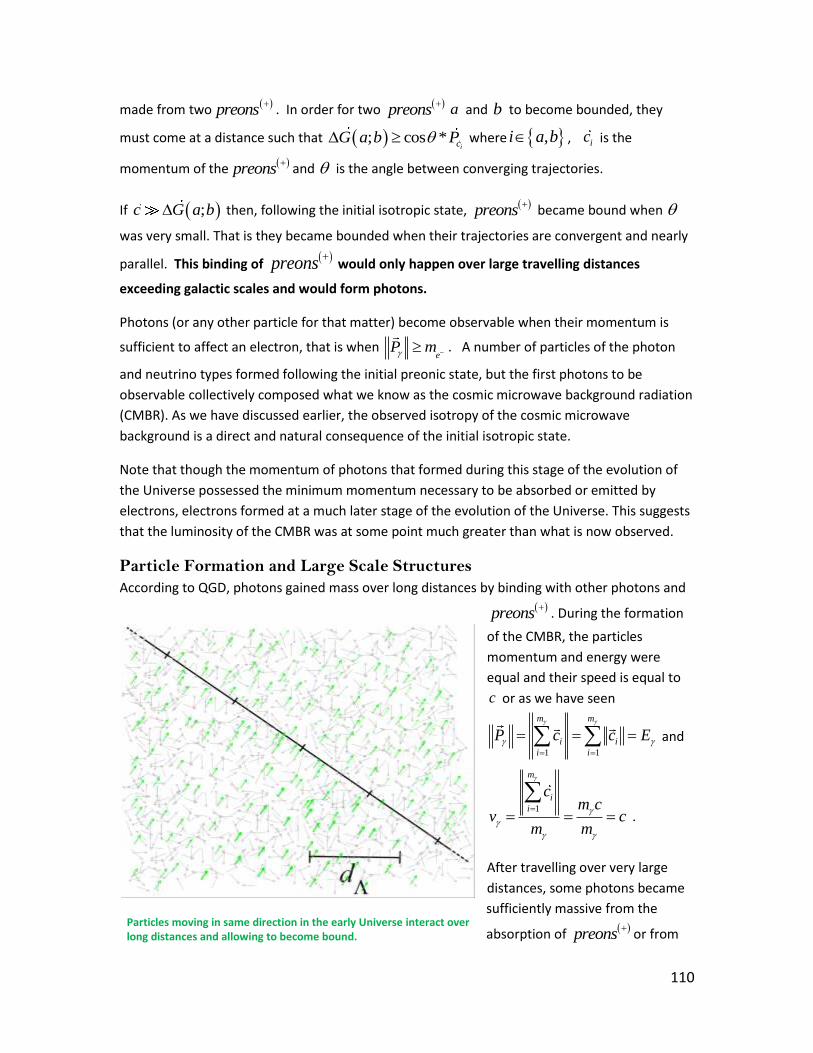
110
made from two preons
. In order for two
preons
a and b to become bounded, they
must come at a distance such that ; cos *icG a b P where ,i a b , ic is the
momentum of the preons
and is the angle between converging trajectories.
If ;c G a b then, following the initial isotropic state, preons
became bound when
was very small. That is they became bounded when their trajectories are convergent and nearly
parallel. This binding of preons
would only happen over large travelling distances
exceeding galactic scales and would form photons.
Photons (or any other particle for that matter) become observable when their momentum is
sufficient to affect an electron, that is when e
P m . A number of particles of the photon
and neutrino types formed following the initial preonic state, but the first photons to be
observable collectively composed what we know as the cosmic microwave background radiation
(CMBR). As we have discussed earlier, the observed isotropy of the cosmic microwave
background is a direct and natural consequence of the initial isotropic state.
Note that though the momentum of photons that formed during this stage of the evolution of
the Universe possessed the minimum momentum necessary to be absorbed or emitted by
electrons, electrons formed at a much later stage of the evolution of the Universe. This suggests
that the luminosity of the CMBR was at some point much greater than what is now observed.
Particle Formation and Large Scale Structures
According to QGD, photons gained mass over long distances by binding with other photons and
preons
. During the formation
of the CMBR, the particles
momentum and energy were
equal and their speed is equal to
c or as we have seen
1 1
m m
i i
i i
P c c E
and
1
m
i
i
cm c
v cm m
.
After travelling over very large
distances, some photons became
sufficiently massive from the
absorption of preons
or from
Particles moving in same direction in the early Universe interact over long distances and allowing to become bound.

111
merging with other photons for them to bind with other massive photons when their trajectory
intersected at larger angles. That is when cos *
;cos *
PG
P
. The momentum of the
resulting particles would be much smaller than their combined individual momenta or energies.
Hence the velocity of the new particles formed in that way would be orders of magnitude slower
than c .
1 1 1 1 1 1
m m m m m m
i i i i i i
i i i i i i
P c c c c c c
and P
vm
and since
P E then v c .
That is how particles with larger masses and subluminal velocity were produced, some many
orders of magnitude slower than c .
Slow massive particles with momentum less than the minimum allowable change in momentum
for an electron are as a consequence not detectable (dark) but they can be indirectly detected
through their
gravitational interactions
with visible matter and
light.
Under the effect
gravitational interaction
(attractive for d d and
repulsive for d d ,
where the threshold
distance 10d Mpc )
condensed into streams
of dark matter which at
their intersection formed
halos. It is from and
within these halos that
progressively more
massive particles formed,
which eventually created
the galaxies and galaxies
clusters.
Under the influence of attractive and repulsive gravity, particles over very large distances form streams of particles. The more massive the particles, the shorter the distance over which the streams are formed and the denser they are.

112
The above figure illustrates streams of dark particles (dark matter), shaped by attractive and
repulsive gravity create the filaments of the observed large scale structure of the Universe.
Galaxy clusters are formed at the intersections of two or more streams.
Since the distance between intersections of filaments within which clusters are formed is
greater than d , galaxies belonging to different clusters gravitationally repel each other and
causing the expansion of the material Universe. The rate at which galaxies recess from one
another is described by the QGD’s
equation for gravity; hence it
increases with distance between
them and with their mass and most
significantly as a function of their
distance from the center of the
Universe. Current theories assume
that the universe is infinite, but if
space is discrete (an axiom of QGD),
then the fundamental elements of
space, the preons
, must obey the
law of conservation, hence there must be a finite number of them, hence the universe must be
spatially finite with a finite number of dimension (three) and a finite amount of matter.
It is important here to emphasize the difference between the expansion of the Universe as it is
currently understood, which implies the expansion of space itself, and the material expansion of
the large scale structure due to repulsive gravity which requires space to remain fixed.
Galaxy Formation, Motion, Shape and Evolution
Once particles started to condense
to form the large scale structures,
the distribution of matter became
anisotropic and as a consequence,
the non-homogeneous distribution
of matter resulted in
heterogeneous gravitational
interactions between structures.
As more matter condensed, the
magnitude of both attractive
gravity from within proto-galaxies
and net repulsive gravity from
matter at distances beyond the
d threshold increased and Andrew Pontzen and Hiranya Peiris, University College London
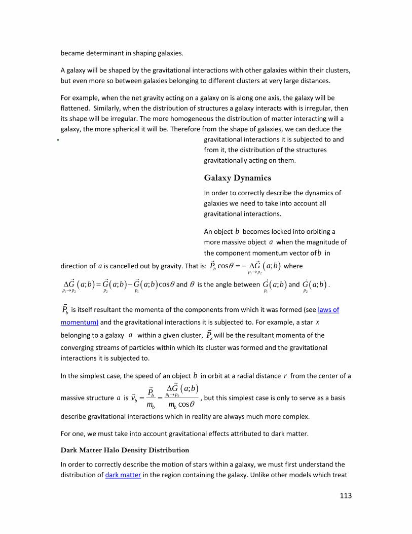
113
became determinant in shaping galaxies.
A galaxy will be shaped by the gravitational interactions with other galaxies within their clusters,
but even more so between galaxies belonging to different clusters at very large distances.
For example, when the net gravity acting on a galaxy on is along one axis, the galaxy will be
flattened. Similarly, when the distribution of structures a galaxy interacts with is irregular, then
its shape will be irregular. The more homogeneous the distribution of matter interacting will a
galaxy, the more spherical it will be. Therefore from the shape of galaxies, we can deduce the
gravitational interactions it is subjected to and
from it, the distribution of the structures
gravitationally acting on them.
Galaxy Dynamics
In order to correctly describe the dynamics of
galaxies we need to take into account all
gravitational interactions.
An object b becomes locked into orbiting a
more massive object a when the magnitude of
the component momentum vector ofb in
direction of a is cancelled out by gravity. That is: 1 2
cos ;bp p
P G a b
where
1 2 2 1
; ; ; cosp p p p
G a b G a b G a b and is the angle between
1
;pG a b and
2
;pG a b .
bP is itself resultant the momenta of the components from which it was formed (see laws of
momentum) and the gravitational interactions it is subjected to. For example, a star x
belonging to a galaxy a within a given cluster, xP will be the resultant momenta of the
converging streams of particles within which its cluster was formed and the gravitational
interactions it is subjected to.
In the simplest case, the speed of an object b in orbit at a radial distance r from the center of a
massive structure a is
1 2
;
cos
p pbb
b b
G a bP
vm m
, but this simplest case is only to serve as a basis
describe gravitational interactions which in reality are always much more complex.
For one, we must take into account gravitational effects attributed to dark matter.
Dark Matter Halo Density Distribution
In order to correctly describe the motion of stars within a galaxy, we must first understand the
distribution of dark matter in the region containing the galaxy. Unlike other models which treat

114
dark matter as an exotic type of matter, QGD predicts that all matter is fundamentally
composed of preons
, themselves dark, which become bounded to form progressively more
massive particles which as we have explained earlier become visible matter when photons they
absorb or emit have at least the minimum momentum necessary to be absorbed by an electron.
This implies that vmm , the rate at which visible matter is created from dark matter, must be
proportional to the dark halo density dm but also that there is a critical density min below
which visible matter cannot form. As a consequence, the density of the dark matter is not
expected to increase as we get closer to the center of a galaxy as dominant dark matter models
predict. Under the influence of gravity, dark matter would concentrate towards the center, but
the higher rate of production of visible matter would tend towards keeping dm below min .
QGD predicts that mindm within a radius
minr d where
mind
is the distance beyond
which mindm . This dynamics which limits the increase of dark matter density towards
the center of a galaxy is consistent with the observed flat dark matter density profiles of
galaxies1617. Thus QGD precludes the formation of the dark matter cusps predicted by dominant
dark matter models (see cuspy halo problem).
Rotation Curve of Galaxies
QGD’s equation for gravity and its predicted for dark particles ( particles for with e
P m )
explain the observed rotation curves of galaxies.
The orbital velocity of a star is ;
cos
bb
b b
G a bPv
m m
where
; ; ;
* *a b a b
G a b G a b G a b
m m k m m d
Note that the p-gravity and n-gravity components of QGD’s equation for gravity
2
;1
a b
d dG a b m m k
must be differentiated separately since gravity is the resultant
effect of the p-gravity force which is a function of mass only while n-gravity force is a function of
both mass and distance. When only taking into account two objects with constant masses, then
16
Moore, Ben; et al. (August 1994). "Evidence against dissipation-less dark matter from observations of galaxy haloes". Nature. 370 (6491): 629–631. Bibcode:1994Natur.370..629M. doi:10.1038/370629a0. 17
Oh, Se-Heon; et al. (May 2015). "High-resolution Mass Models of Dwarf Galaxies from LITTLE THINGS". The Astronomical Journal. 149 (6): 180. arXiv:1502.01281. Bibcode:2015AJ....149..180O. doi:10.1088/0004-6256/149/6/18

115
; 0G a b and ; ;G a b G a b , and objects behave as if governed by Newtonian
gravity with gravity diminishing as a function of the square of the distance and
;b
b
G a bv
m
and
;a
a
G a bv
m
. The action is the same but where Newtonian gravity
is strictly attractive with variations due to variations in distance between a andb , QGD
attributes the change in gravity variations in repulsive gravity (n-gravity) as a function of
distance.
In order to describe the rotation curve of a galaxy, we need to consider the influence of both
visible and dark matter. That is, if aR is a spherical region of space with radius r d which
center coincides with the center of a galaxy a and then the mass of matter within aR is
aR a dmm m m , where am and dmm are respectively the amount of visible matter and dark
matter in aR , then ; ;
a aR R
b
b
G m b G m bv
m
.
;aR dm bG m b m m k and since 24
dmR dmm r ,.
2 3
; ; ;
4 2
a a a
dm b dm b
G R b G R b G R b
r m k r m
and
2 3
2
4 2
42
b dm dm
dm
v r k r
rr k
And if the density of dark matter is inversely proportional to the square of the distance from the
center of the galaxy then 2
24 4
2 2
dmb dm
r rv r k k
r
, hence the observed
flattening of the rotation curve of galaxies.
116
Recession Speed between Large Structures
The rate at which large structures accelerate away from each other is proportional to the
variation in the gravitational repulsion between two positions and is given by
; ;a b a b
a b
a b
G R R G R Rv v
m m
.
If the universe evolved from an isotropic state such as we described earlier, then the speed of a
structure b relative to a structure a is equal to the total acceleration between d , the
threshold distance at which gravity becomes repulsive, and d the distance between the
structures a and b . That is,
; ;
;
d d
a b a b dd d a b
a b a brel
da b a b
G R R G R Rm m
v v v G R Rm m m m
.
The acceleration from a galaxy from a large structure is independent of its mass but only
dependent on the mass of the structure it is receding from.
Like acceleration from attractive gravity, acceleration from repulsive gravity is directly
proportional to the distance. The derivative of QGD’s equation for gravity over distance gives
the gravitational acceleration over a distance or a bR Rv m d .
Then a b a bR R R R
relv v v m m d where d may be understood as the proper distance
between aR and bR .
The acceleration of the rate of recession between a andb is
2 2
2a b a brel R R R R
d dv m m m m d
However, the recession speed between two structures does not only depend on the distance
and masses of the structures, but on all masses and structures each interact with, that is, it
depends on the gravitational interactions with the rest of the universe, therefore, it depends on
each galaxies positions relative to the center of the galaxy. This is measured using the
cosmological redshift as discussed in the following section.
Expansion Rate of the Material Universe and the Cosmological Redshift
According to QGD, space is composed of a finite number fundamental discrete units, preons
, which makes space a static structure through in which all matter exists. Hence space is finite
and must have a center and an edge.

117
Material structures are strictly kinetic and as we have seen in previous sections gravitationally
attract or repel one another depending on whether the distances that separate them is smaller
or greater than the threshold distance d .
We define the cosmological acceleration as the effect of gravity on structures at a scale at which
structures are separated by distances greater than the threshold distance beyond which gravity
becomes repulsive or d d . At the cosmological scale, since gravity is repulsive, the structures
accelerate away from the center of the Universe at a rate that is proportional to their distance
from the center and the inversely proportional to their shortest distances from the edge of the
Universe.
For an object a at a distance r from the center of the Universe and Ud , the diameter of the
universe, we find that 1 2; ;a R a R aP G m m G m m where
x x
UR R
U
mm vol
Vol .
Observationally, objects at the cosmological scale that are closer than we are to the center of
the universe will appear blueshifted relative to light from the center of our galaxy and objects
that are further than we ware from the center of the Universe will appear redshifted relative to
it.
However, since the cosmological acceleration affects a galaxy as a whole with negligible
differences on individual components of a galaxy, we would observed within a galaxy stars that
may be redshifted or blueshifted relative to a reference star depending on whether the
observed star is respectively closer or further from the center of the galaxy.
Black Holes and Black Holes Physics
QGD predicts the existence of structures which exerts such gravitational pull that photons
cannot escape. But contrary to the classical black holes predicted by relativity, the black holes
predicted by quantum-geometry dynamics are not singularities. The QGD exclusion principle
which states that a preon
cannot be occupied by more than one
preon
implies that
quantum-geometrical space imposes a limit to the density any structure can have. The density of
black holes is also limited by the fact that preons
, being strictly kinetic, they must have
enough space to keep in motion. It follows that black must have very large yet finite densities.
Angle between the Rotation Axis and the Magnetic Axis
The effect of the helical motions of the electrons in direction of the rotation of a body adds up
so that, at a large scale, the body behaves as a single large electron which though helical
trajectory around the body interacts with the neighbouring preonic region to generated a
magnetic field.
Since the magnetic field is the result of the polarization of free preons
along the loops of the
helical trajectory, and since the inclination of these loops increases with the speed of rotation,

118
so does the angle between these loops and the axis of rotation increases. It follows that the
angle between the axis of rotation and the magnetic axis for bodies of given material
composition is proportional to the speed of rotation about its axis and its diameter.
This angle between the axis of rotation and the magnetic axis is small for slowly rotating bodies
but can never be so small that the axes coincide. From the above, it also follows that a faster
rotation not only implies a larger the angle between the rotation axis and the magnetic axis is,
but also a flattening of the magnetic field and an increase in its intensity.
The Inner Structure of Black Holes
To understand the structure of a black hole we will look at what happens to a photon when it is
captured by it the gravitational pull.
The model for light refraction that we introduced in earlier articles can be applied directly to
photon moving through a black hole. Since we assume that the black hole is extremely massive,
its trajectory will bring it towards the center of the black hole.
When moving along the magnetic axis of the black hole, the component preons
of the
preon
pairs of the photon are pulled away from each other, splitting the photon into free
preons
which may or not recombine into neutrinos. This works as follow:
As we have seen earlier in this book, the force binding the preons
of a
preon
pairs is
gravitational. The QGD gravitational interaction between particles at the fundamental scale is
2
2; a b
d dG a b m m k
, and since a and b are preons
, 1a bm m and since
1d , the binding force between two preons
of a
preon
pair is equal to 1k .
For a photon moving along the magnetic axis, we have and 1 2 1 1; ; 1G p R G p R k
where 1p
and 2p
are the component preons
of a
preon
pair of a photon.
The regions 1R and 2R , on each side of the black hole axis are equally massive regions. If we
call 1Rand 2R the regions each side of 1p
when the photon’s trajectory is aligned with the
black hole axis then 2 1R R and 1 2 1 1; ; 1G p R G p R k
. Similarly, if we call 1R and
2R the region on the each side 2p
then 1 2R R and 2 1 2 2; ; 1G p R G p R k
. So
the force pulling the preons
of
preon
pairs being greater than the force that binds them,
the preon
pairs are split into single
preons
.

119
How do we that the gravitational forces within a black hole are sufficiently strong to cause the
photons to be broken down into preons
? If the gravitational forces within the black hole
were not enough to breakdown the photons, then photons moving along a black hole axis would
escape into space making the black hole visible. Since black holes do not emit light, then the
gravitational interactions must be strong enough to break photons down into preons
and
neutrinos.
The image above shows how a simple two preons
photon is split into two free
preons
which because of the electro-gravitational interactions move back toward the magnetic axis.
But, because the quantum-geometrical space occupied by the black holes is densely populated
by particles which affect randomly the trajectories of the single preons
, our two
preons
arrive at the magnetic axis of the black hole at different positions. And if they are in close
enough proximity, the single preons
will combine to form a neutrino which structure, not
being made of preons
pairs, remains structurally unaffected by the intense gravitational
interactions within the black hole.
Once the trajectories of the preons
or the neutrino coincides with the magnetic axis of the
black hole, the preons
or neutrinos will move through the center of the black hole and will
exit it.
Preons
and neutrinos can escape the gravitation of the black hole because
gravitational interactions, though it affects the directions of preons
, doesn’t change their
momentums which, as we have seen in earlier articles is fundamental and intrinsic (the
momentum of a preon
is c where c is momentum vector of a
preon
).
It follows, that all matter that falls into a black hole will be similarly disintegrated into preons
and neutrinos, which will exit the black hole. The black hole will thus radiate preons
and
neutrinos, in jets at both poles of their magnetic axis of rotation. Since preons
and neutrinos
120
interact too weakly with instruments to be detected by our instruments, they are invisible to
them. In order to see the preons
-neutrinos jets from a black hole, instruments may need
detectors larger than our solar system. However, the jets can be observed indirectly when they
interact with large amount of matter when the polarized preons
and neutrinos they contain
impart it with their intrinsic momentum. It is worth noting that polarized preons and neutrinos
jets, as described by QGD, would contribute to the observed dark energy effect.
Based on QGD’s model of the black hole, we can predict that the preons
/neutrino jets will
form an extremely intense polarized preons
field along the magnetic axis creating the
equivalent of a repulsive electromagnetic effect at both poles. The polarized preonic field would
repulse all matter on their path, which may explain the shape of galaxies.
From what we have discussed in the preceding section, we can define a black hole as an object
which mass is such that it can breakdown all matter, including photons, into preons
.
Therefore, any emission by a black hole being preonic, they are not visible. However, intense
preonic fields (which as we have seen are essentially intense magnetic fields), will impart
momentum to particles and structures, bringing them into excited states from which they emit
photons.
The QGD model of the physics of black hole has another important implication. The preons
and neutrinos resulting from the breakdown of a particle or structure are indistinguishable from
the preons
or neutrinos resulting from the breakdown of any other particle or structure. This
means, if QGD is correct, that all information about the original particle or structure is lost
forever. That said, since this consistent from QGD’s axioms set and since, unlike quantum
mechanics, QGD does not require that information be preserved, the loss of information it
predicts does not lead to a paradox ( see this article for an excellent introduction to subject).
Density and Size of Black Holes
QGD predicts that black holes are extremely dense but not infinitely so. Considering that
preons
are strictly kinetic and that no two can simultaneously occupy any given preons
then
1 1max
22BH
preondensity or
preons
. It follows that
min 2BH BHVol m preons
or, since
preon
is the fundamental unit of space, we can simply write min 2BH BHVol m for the
minimum corresponding radius 33
min2
BHBH
mr
.
121
For the radius of the black hole predicted to be a the center of our galaxy, 64*10BHm M
and 2
33
min 1.24*102
BHBH
mr M
where the mass is expressed in preons
and radius
in preons
. Though converting this into conventional units requires observations to
determine the values of the QGD constants k and c , using relation between QGD and
Newtonian gravity, we also predict that the radius within which light cannot escape a massive
structure is qgd const
Mr G
c where constG is used to represent the gravitational constant. Since
the Schwarzschild radius for a black hole of mass BHM is 2
BHs const
Mr G
c then
qgd sr cr .
Using qgdr to calculate
qgdr the angular radius of the shadow of Sagitarius A*, the black hole at
the center of our galaxy, where 64*10BHM M we get 526.64*10qgdr
arcseconds which
is about 10 times the angular radius calculated using the Schwarzschild radius which i 627.6*10
sr arcseconds. This prediction will be tested in the near future by the upcoming
observations by the Event Horizon Telescope.
Neutron Stars, Pulsars and Other Supermassive Structures
When the mass of a structure is sufficient to bind photons, but insufficient to breakdown
photons, electrons and positron, we get a stellar structure which can emit these particles.
The internal gravitational interactions will redirect particles towards the magnetic axis of the
stellar structures where, when its trajectory coincides with an axis, the gravitational force from
the stellar object acting on the particles will cancel out and the particle will escape the object
into outer space. Such structures may correspond to what we call neutron stars. So what
distinguishes neutron stars from black holes is that we have 1 2 1 1; ; 1G p R G p R k
and 2 1 2 2; ; 1G p R G p R k
. That is, the gravitational force within the neutron star
which acts on particles is insufficient to breakdown photon, electron and positrons.
Another prediction is that distinguishes quantum-geometry dynamics is that neutron stars are
not composed of neutrons. The internal gravitational forces being such that they would break
down all particles into neutrinos, photons, electrons and positrons.
Pulsars
When a neutron star rotates at a sufficiently high rate, it interacts with the preonic field in such
a way that it creates an intense magnetic field. Such magnetic field will be sufficiently strong to
curve the trajectory of all neutrinos, photons, electrons and positrons that move past its surface
back into pulsar. Particles that move along its axis of rotation, along which the electromagnetic
122
force cancel out, will escape at the magnetic poles producing the known bidirectional emission
characteristic of pulsars.
The Preonic Universe
According to the principle of strict causality we can deduce the following:
Preons
and
preons
, are fundamental. As such and in accordance with the
fundamentality theorem, they have no components; hence they require no pre-existing
conditions to exist. From this and to be in accordance with the Law of Conservation, all
preons and
preons always existed.
That is, preons
and preons
not only existed at the origin of the Universe. They are
the origin of the Universe.
It follows that in its initial phase, the Universe consisted of preons
uniformly
distributed throughout the entire quantum-geometric space of the Universe; the
preonic universe.
The theory proposes that the n-gravity and p-gravity fields were in perfect equilibrium.
That is:
2 2( ) / 2 ( ) /2U U U Uk m m Vol Vol
Where Um is the mass of the preonic universe and UVol is the number of preons
its
space is composed of. But since 2
lim 0x
x
x
, at the macroscopic scale, the relative
value of Um and UVol become negligible and we can simply write18:
2 2/ 2 / 2U Ukm Vol
Also, from the QGD definitions of heat, temperature and entropy we know that, since in
the primordial universe contained only free preons
, the heat it contained was equal
to its energy, that is 1
Um
i U
i
Heat c m c
, its temperature was U
U
m c
Vol and its entropy
being the difference between its energy and heat, and heat and energy being equal in
the preonic universe, its entropy was equal to zero.
18
Since QGD implies that all quantities are finite, even mathematical quantities, represents the largest theoretical quantity of any physical property. In this equation it may be taken as the number of n-gravity interactions in the universe.

123
Interestingly, since 2
U UVol km the temperature of the preonic universe is given by
.
Hence, the temperature of the preonic universe is a ratio of and ; the two
fundamental constants of quantum-geometry dynamics.
Future Evolution of the Universe
If QGD’s description of the universe is correct, then most matter would eventually
collapse into black holes where it would be broken down in into preons
which would
be emitted and would reseed the universe; resetting the initial isotropic state.
One question remains. What will happen to the galaxies that will be pushed to the limits
of the universe?
2
U
U
m c c
kkm
c k

124
Some Thoughts about the Future of QGD
SECTION WILL BE ADDED IN A LATER UPDATE