introduction to some applied statistical methods and how
TRANSCRIPT

電子郵件:[email protected]個人網頁:http://www.stat.sinica.edu.tw/hsinchou/電話:02-27835611 轉 113傳真:02-27831523
Introduction to some applied statistical methods and how to perform them in R
楊欣洲、林胤均、黃美菊、陳佳煒、朱是鍇、梁佑任
中央研究院統計科學研究所
2016-08-12 @ 統計研習營(中研院統計所) 1

Contents
時間 軟體簡稱 R function 助教
14:00 – 14:50 Introduction tobiostatistical methods
--- Dr. 楊欣洲
休息十分鐘
15:00 – 15:25 contingency table analysis; logistic regression;
ordinal logistic regression
chisq.test;glm;vglm;
Mr.林胤均
15:25 – 15:50 correlation analysis;linear regression;
analysis of variance; survival analysis
cor;lm; summary;
anova;bpcp package: bpcp;
survival package: Surv, survfit, coxph;
Miss.黃美菊
討論與休息十分鐘
16:00 – 16:25 discriminant analysis;cluster analysis
lda {MASS};hclust {stats};
Mr.陳佳煒
16:25 – 16:50 principal component analysis; partial least square analysis
prcomp;opls;
Mr. 朱是鍇
綜合討論 2

Pokemon X vs. Y
3
The differences: Mega Mewtwo X, becomes psychic/fighting type, and its attack stat increases. In addition, it also gains the "steadfast" ability, which increases its speed whenever it flinches in battle. Mega Mewtwo Y increases its special attack significantly and it gains the "insomnia" ability—as it suggests, this ability prevents Mewtwo from falling asleep.
http://kotaku.com/which-version-should-you-buy-pokemon-x-or-pokemon-y-1444397068
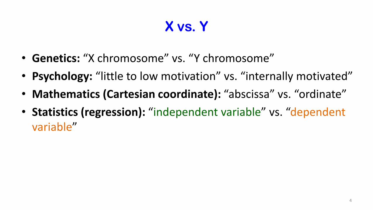
X vs. Y
• Genetics: “X chromosome” vs. “Y chromosome”
• Psychology: “little to low motivation” vs. “internally motivated”
• Mathematics (Cartesian coordinate): “abscissa” vs. “ordinate”
• Statistics (regression): “independent variable” vs. “dependent variable”
4

Variable/Data type
• Categorical data (i.e., qualitative or nominal data) [e.g., sex, nucleotide type, blood type, and affection status]
• Ordinal data [e.g., disease severity, cancer stage, socioeconomic status, and satisfaction level in questionnaire]
• Numerical data (i.e., quantitative data)– Discrete [e.g., number of nucleotides, number of patients,
and frequency of clinic visits]– Continuous [e.g., gene expression, body temperature,
body mass index (BMI), and survival time]
5

Outline
• correlation analysis• linear regression• analysis of variance• contingency table analysis• logistic regression• ordinal logistic regression• survival analysis• discriminant analysis• cluster analysis• principal component analysis• partial least square discriminant analysis• three data sets
6

Outline
• correlation analysis• linear regression• analysis of variance• contingency table analysis• logistic regression• ordinal logistic regression• survival analysis• discriminant analysis• cluster analysis• principal component analysis• partial least square discriminant analysis• three data sets
7
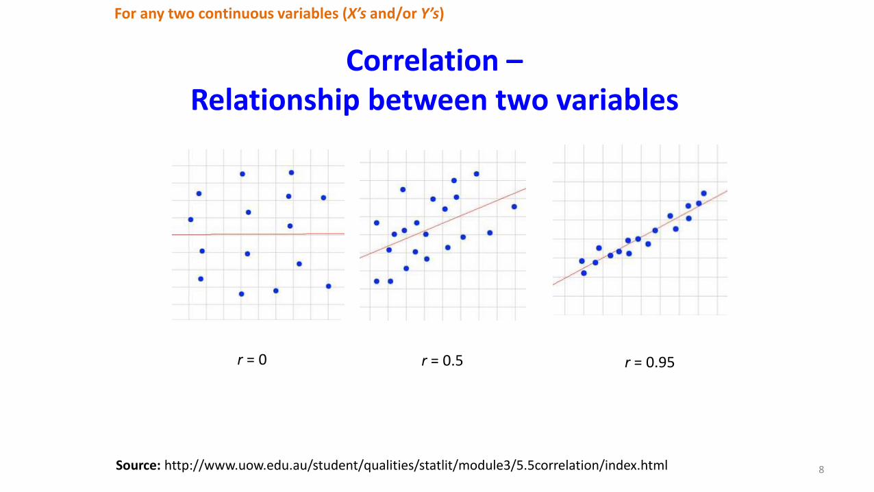
Correlation –Relationship between two variables
For any two continuous variables (X’s and/or Y’s)
8Source: http://www.uow.edu.au/student/qualities/statlit/module3/5.5correlation/index.html
r = 0 r = 0.5 r = 0.95

Correlation –Pearson correlation coefficient
For any two continuous variables (X’s and/or Y’s)
9Ps: other correlation measures such as Spearman correlation, Kendall tau, …

Outline
• correlation analysis• linear regression• analysis of variance• contingency table analysis• logistic regression• ordinal logistic regression• survival analysis• discriminant analysis• cluster analysis• principal component analysis• partial least square discriminant analysis• three data sets
10

Regression –Relationship between ≥ 2 variables
• Simple linear regression:• Relationship between regression and correlation: • Multiple linear regression:
11
Y: continuous, X: continuous and/or categorical
Source: http://www.uow.edu.au/student/qualities/statlit/module3/5.5correlation/index.html
Ƹ𝑟 = 0 Ƹ𝑟 = 0.5 Ƹ𝑟 = 0.95
መ𝛽 = Ƹ𝑟 ×𝑆𝑑(𝑌)
𝑆𝑑(𝑋)
𝑌𝑖 = 𝛼 + 𝛽𝑋𝑖 + 𝜀𝑖
𝑌𝑖 = 𝛼 + 𝛽1𝑋𝑖 +⋯+ 𝛽𝑝𝑋𝑖 + 𝜀𝑖
Association between Y and X

Regression – A toy example
12
Y: continuous, X: continuous and/or categorical
Source: http://www.uow.edu.au/student/qualities/statlit/module3/5.5correlation/index.html
• The example about the correlation between the age and weight of the children
ො𝛼መ𝛽
Question: X and Y are uncorrelated?It is equivalent to test H0: 𝜷 = 𝟎
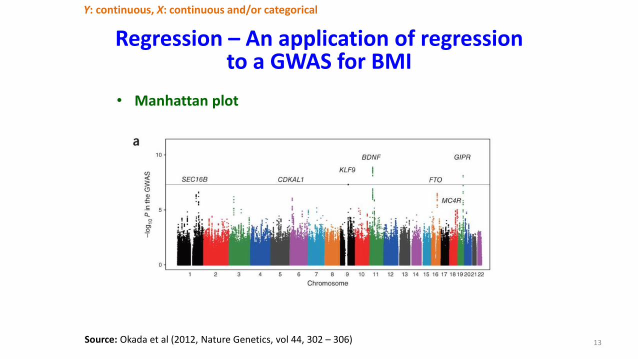
Regression – An application of regression to a GWAS for BMI
13
Y: continuous, X: continuous and/or categorical
Source: Okada et al (2012, Nature Genetics, vol 44, 302 – 306)
• Manhattan plot

Regression – SNP-NP Interaction
• Illustration of an interaction
14
Notation: Y denotes a quantitative trait and X’s are additive-effect SNPs
Y
X1=AA=0
X2X2=BB=0 X2=Bb=1 X2=bb=2
X1=Aa=1
X1=aa=2No interactionY
X1=AA=0
X2X2=BB=0 X2=Bb=1 X2=bb=2
X1=Aa=1
X1=aa=2
Interaction
𝑌𝑖 = 𝛼 + 𝛽1𝑋1𝑖 + 𝛽2𝑋2𝑖 + 𝛽3(𝑋1𝑖𝑋2𝑖) + 𝜀𝑖
Y: continuous, X: continuous and/or categorical

Outline
• correlation analysis• linear regression• analysis of variance• contingency table analysis• logistic regression• ordinal logistic regression• survival analysis• discriminant analysis• cluster analysis• principal component analysis• partial least square discriminant analysis• three data sets
15
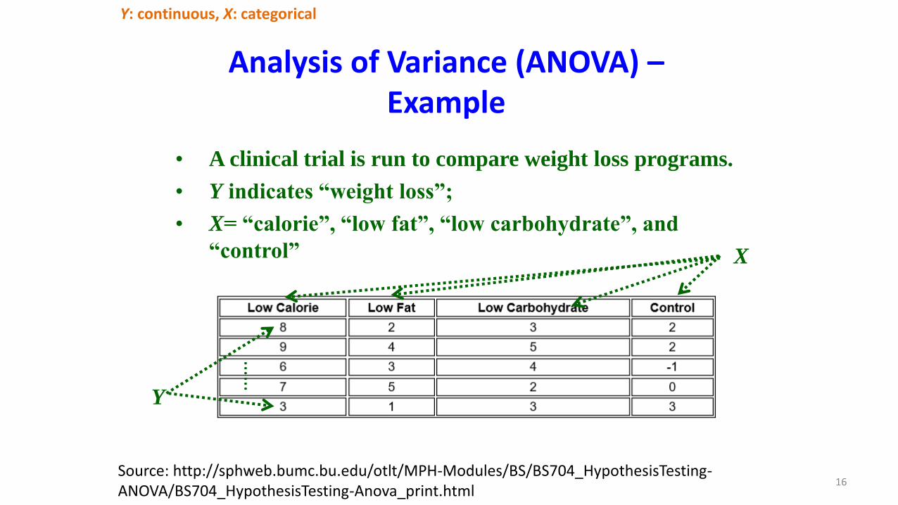
Analysis of Variance (ANOVA) –Example
16
Y: continuous, X: categorical
• A clinical trial is run to compare weight loss programs.
• Y indicates “weight loss”;
• X= “calorie”, “low fat”, “low carbohydrate”, and
“control”
Source: http://sphweb.bumc.bu.edu/otlt/MPH-Modules/BS/BS704_HypothesisTesting-ANOVA/BS704_HypothesisTesting-Anova_print.html
Y
X
……

Analysis of Variance (ANOVA) –Linear model
• Linear model:
• Hypothesis test:
17
𝐻0: 𝛼1 = 𝛼2 = ⋯ = 𝛼𝑏 = 0 or 𝐻0: 𝜇1 = 𝜇2 = ⋯ = 𝜇𝑏 = 𝜇
𝑌𝑥𝑗 = 𝜇 + 𝛼𝑥 + 𝜀𝑥𝑗 , 𝑥 = 1,⋯ , 𝑏(= 4), 𝑗 = 1,⋯ , 𝑛(= 5)
YY
XX
Source: https://en.wikipedia.org/wiki/Analysis_of_variance
Y: continuous, X: categorical

Analysis of Variance – Microarray array quality control (MAQC) study
18Source: Patterson et al (2006, Nature Biotechnol, vol 24, 114- – 1150)
Y: continuous, X: categorical
Outline
• correlation analysis• linear regression• analysis of variance• contingency table analysis• logistic regression• ordinal logistic regression• survival analysis• discriminant analysis• cluster analysis• principal component analysis• partial least square discriminant analysis• three data sets
19

Contingency table analysis –Chi-square Test (1)
• The 1st successful GWAS identified a SNP on complement factor H gene for age-related macular degeneration (AMD) (Kline et al, 2005, Science, vol 308, 385 – 389)
20
X1: Categorical; X2: Categorical

Contingency table analysis –Chi-square Test (2)
• SNP rs380390
AMD
Genotype Alleletype
CC CG GG Total C G Total
Y 49 37 10 96 135 57 96*2
N 5 26 19 50 36 64 50*2
54 63 29 146 171 121 292
21
𝑋2 =(𝑂𝑌,𝐶−𝐸𝑌,𝐶)
2
𝐸𝑌,𝐶+(𝑂𝑌,𝐺−𝐸𝑌,𝐺)
2
𝐸𝑌,𝐺+(𝑂𝑁,𝐶−𝐸𝑁,𝐶)
2
𝐸𝑁,𝐶+(𝑂𝑁,𝐺−𝐸𝑁,𝐺)
2
𝐸𝑁,𝐺~𝜒2
1
𝐸𝑌,𝐶 = 𝑂+,+ × ( Τ𝑂+,𝐶 𝑂+,+) × ( Τ𝑂𝑌,+ 𝑂+,+)
X1: Categorical; X2: Categorical
P-value = 3.3*10^-8
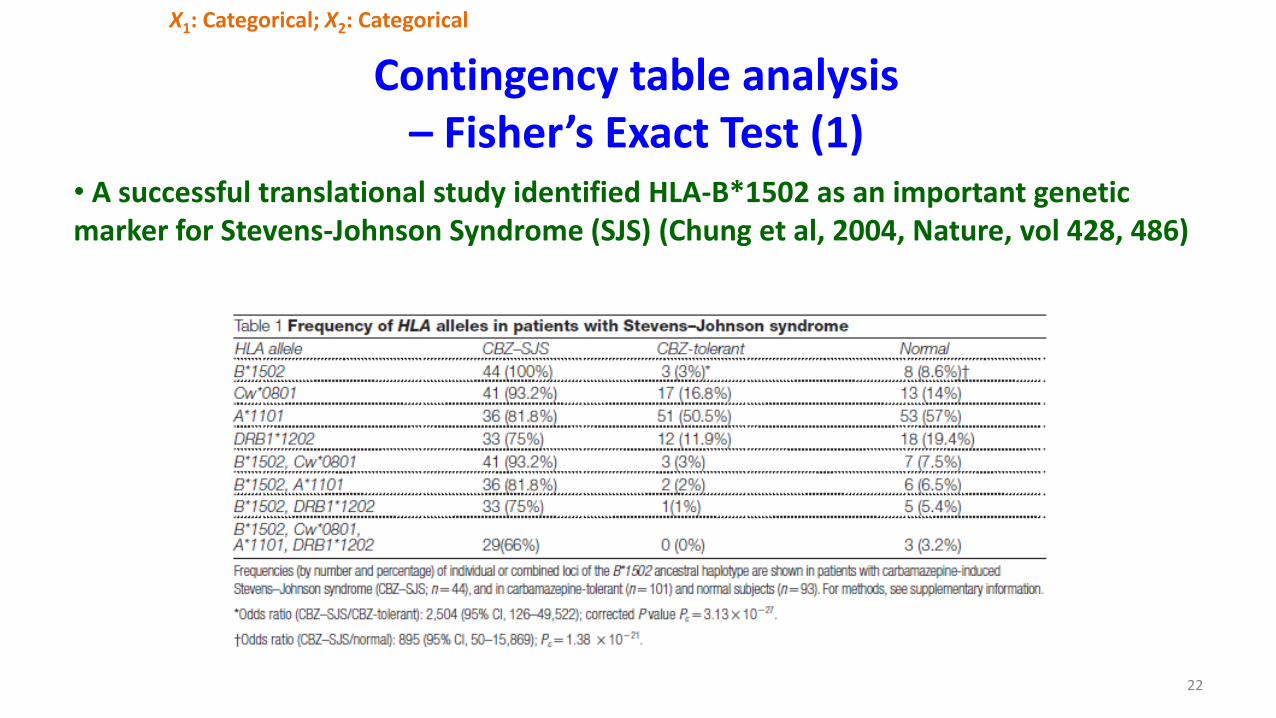
Contingency table analysis – Fisher’s Exact Test (1)
• A successful translational study identified HLA-B*1502 as an important genetic marker for Stevens-Johnson Syndrome (SJS) (Chung et al, 2004, Nature, vol 428, 486)
X1: Categorical; X2: Categorical
22

Contingency table analysis –Fisher’s Exact Test (2)
• A genetic marker for Stevens-Johnson Syndrome (SJS)
SJS
HLA-B
B*1502
(yes)
B*1502
(no)
CBZ-SJS 44 0 44
CBZ-tolerant 3 98 101
145
23
X1: Categorical; X2: Categorical
Note: Hypergeometric distribution is used to calculate p-value of Fisher’s exact test.

Outline
• correlation analysis• linear regression• analysis of variance• contingency table analysis• logistic regression• ordinal logistic regression• survival analysis• discriminant analysis• cluster analysis• principal component analysis• partial least square discriminant analysis• three data sets
24

Logistic regression – Concept
Y: Binary; X’s: Categorical and/or continuous
25Source: Lever et al (2016, Nature Methods, vol 13, 541 – 542)

Logistic regression
Case 1:
• Y = 1 indicates “hypertensive case” and Y = 0 indicates “control”
• X1 indicates age & X2 indicates BMI
Case 2:
• Y = 1 indicates “hypertensive case” and Y = 0 indicates “control”
• X1 indicates age & X2 indicates a SNP (genotype: AA, AB, BB)
• I1 = 1 if X2 = AA; =0, otherwise. I2 = 1 if X2 = AB, =0, otherwise.
26
ln𝑃 𝑌 = 1 𝑋
1 − 𝑃 𝑌 = 1 𝑋= 𝑙𝑜𝑔𝑖𝑡 𝑃 𝑌 = 1 𝑋 = 𝛽0 + 𝛽1𝑋1 + 𝛽2𝑋2 + 𝛽3𝑋1𝑋2
ln𝑃 𝑌 = 1 𝑋
1 − 𝑃 𝑌 = 1 𝑋= 𝑙𝑜𝑔𝑖𝑡 𝑃 𝑌 = 1 𝑋 = 𝛽0 + 𝛽1𝑋1 + 𝛽2𝐼1 + 𝛽3𝐼2
Y: Binary; X’s: Categorical and/or continuous
Association between disease status and risk factor

Outline
• correlation analysis• linear regression• analysis of variance• contingency table analysis• logistic regression• ordinal logistic regression• survival analysis• discriminant analysis• cluster analysis• principal component analysis• partial least square discriminant analysis• three data sets
27

Ordinal logistic regression
Y: Ordinal; X’s: Categorical and/or continuous
28
ln𝑃 𝑌 ≥ 𝑎 𝑋
1 − 𝑃 𝑌 ≥ 𝑎 𝑋= 𝛽0,𝑎 + 𝛽1𝑋1 +⋯+ 𝛽𝑝𝑋𝑝
• Regression model:
• Example: Y indicates cancer stage 1, 2, 3, or 4.
Severity increase as cancer stage increases.
Association between disease severity and risk factor(s)

Outline
• correlation analysis• linear regression• analysis of variance• contingency table analysis• logistic regression• ordinal logistic regression• survival analysis• discriminant analysis• cluster analysis• principal component analysis• partial least square discriminant analysis• three data sets
29

30
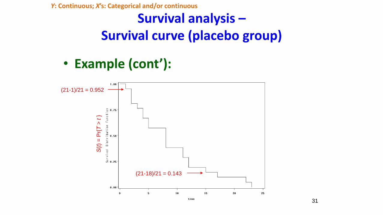
Survival analysis –An example of clinical trial
• Example (Freireich et al, 1963): The remission times (in weeks) of 42 patients with acute leukemia were reported in a clinical trial undertaken to assess the ability of 6-MP (a drug) to maintain remission. Each patient was randomized to receive either 6-MP or a placebo; there were 21 patients in each group. The study was terminated after 1 year. Data from 21 placebo patients: 1, 2, 2, 2, 3, 4, 4, 5, 5, 8, 8, 8, 8, 11, 11, 12, 12, 15, 17, 22 and 23.
Y: Continuous; X’s: Categorical and/or continuous
31
Survival analysis –Survival curve (placebo group)
• Example (cont’):
(21-1)/21 = 0.952
(21-18)/21 = 0.143
S(t
) =
Pr{
T>
t}
Y: Continuous; X’s: Categorical and/or continuous
32
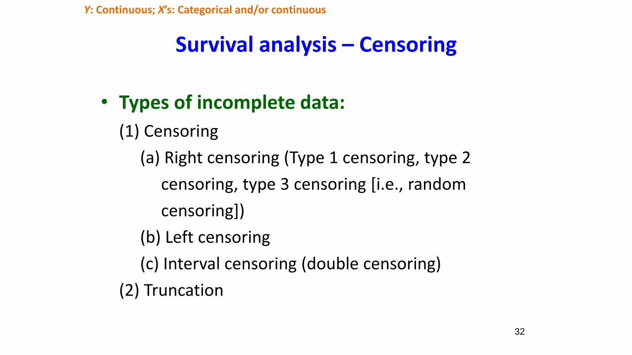
Survival analysis – Censoring
• Types of incomplete data:
(1) Censoring
(a) Right censoring (Type 1 censoring, type 2
censoring, type 3 censoring [i.e., random
censoring])
(b) Left censoring
(c) Interval censoring (double censoring)
(2) Truncation
Y: Continuous; X’s: Categorical and/or continuous

33
Survival analysis – Reasons to censoring
• Reasons:
(1) Loss to follow-up
(2) Dropout event
(3) Termination of the study (for data analysis at
a predetermined time)
(4) Death due to a cause not under investigation
(e.g., suicide)
Y: Continuous; X’s: Categorical and/or continuous

34
Survival analysis –An example of clinical trial (treatment group)
• Example (Freireich et al, 1963):
• Data from 21 placebo patients: 1, 2, 2, 2, 3, 4, 4, 5, 5, 8, 8, 8, 8, 11, 11, 12, 12, 15, 17, 22 and 23;
• Data from 21 6-MP patients: 6, 6, 6, 7, 10, 13, 16, 22, 23, 6+, 9+, 10+, 11+, 17+, 19+, 20+, 25+, 32+, 32+, 34+ and 35+.
Y: Continuous; X’s: Categorical and/or continuous
+ indicates a censored event

35
Survival analysis –Kaplan Meier estimate (two groups)
• Example (cont’):
S(t
) =
Pr{
T>
t}
S(6) = Pr{T > 6 } = 18/21
S(7) = Pr{T > 7 | T > = 7} Pr{T > 6 } = 16/17 × 18/21
Y: Continuous; X’s: Categorical and/or continuous

36
Survival analysis –Cox proportional hazards model
𝜆 𝑡; 𝑥 = 𝜆0 𝑡 exp(𝛼 + 𝛽1𝑋1 +⋯+ 𝛽𝑝𝑋𝑝)
𝜆 𝑡; 𝑥 =𝑓(𝑡; 𝑥)
1 − 𝐹(𝑡; 𝑥)=𝑓(𝑡; 𝑥)
𝑆(𝑡; 𝑥)
• Hazard rate:
• Cox regression:
Association between hazard and risk factor
Y: Continuous; X’s: Categorical and/or continuous

Outline
• correlation analysis• linear regression• analysis of variance• contingency table analysis• logistic regression• ordinal logistic regression• survival analysis• discriminant analysis• cluster analysis• principal component analysis• partial least square discriminant analysis• three data sets
37

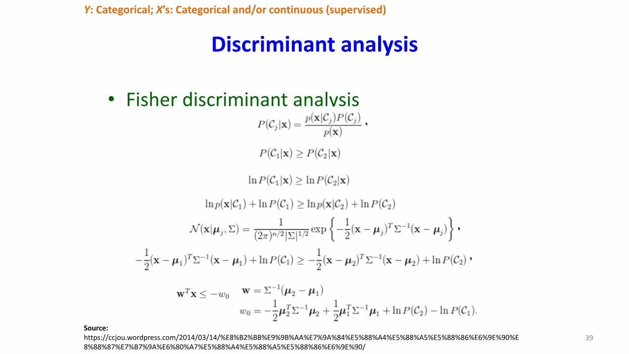
Discriminant analysis
• Fisher discriminant analysis
Source: https://ccjou.wordpress.com/2014/03/14/%E8%B2%BB%E9%9B%AA%E7%9A%84%E5%88%A4%E5%88%A5%E5%88%86%E6%9E%90%E8%88%87%E7%B7%9A%E6%80%A7%E5%88%A4%E5%88%A5%E5%88%86%E6%9E%90/
38
Y: Categorical; X’s: Categorical and/or continuous (supervised)
Discriminant analysis
• Fisher discriminant analysis
Source: https://ccjou.wordpress.com/2014/03/14/%E8%B2%BB%E9%9B%AA%E7%9A%84%E5%88%A4%E5%88%A5%E5%88%86%E6%9E%90%E8%88%87%E7%B7%9A%E6%80%A7%E5%88%A4%E5%88%A5%E5%88%86%E6%9E%90/
39
Y: Categorical; X’s: Categorical and/or continuous (supervised)
Outline
• correlation analysis• linear regression• analysis of variance• contingency table analysis• logistic regression• ordinal logistic regression• survival analysis• discriminant analysis• cluster analysis• principal component analysis• partial least square discriminant analysis• three data sets
40

Cluster analysis
• 9 AITL patients from this study (PAT1 –PAT9)
• 6 AITL patients from GSE6338 (AITL1 – AITL6)
• 5 normal control samples from this study (CD4+)
• exome and transcriptome sequencing
Source: Yoo et al (2014, Nature Genetics, Vol 46, 371 – 375)41
X’s: Categorical and/or continuous (unsupervised)

Outline
• correlation analysis• linear regression• analysis of variance• contingency table analysis• logistic regression• ordinal logistic regression• survival analysis• discriminant analysis• cluster analysis• principal component analysis• partial least square discriminant analysis• three data sets
42

Principal component analysis (PCA)
• Principal components (PCs):
– The 1st PC = Linear combination ℓ1′𝜲 that maximizes Var ℓ1
′𝜲subject to ℓ1
′ℓ1 = 1
– The 2st PC = Linear combination ℓ2′𝜲 that maximizes Var ℓ2
′𝜲subject to ℓ2
′ℓ2 = 1 and Cov ℓ1′𝜲, ℓ2
′𝜲 = 𝟎
– …
• Eigenvalue and eigenvector of variance-covariance matrix
43
Multiple or high-dimensional X’s
𝑌1 = ℓ1′𝜲 = ℓ11𝑋1 + ℓ21𝑋2 +⋯+ ℓ𝑝1𝑋𝑝
𝑌2 = ℓ2′𝜲 = ℓ12𝑋1 + ℓ22𝑋2 +⋯+ ℓ𝑝2𝑋𝑝
⋮
𝑌𝑝 = ℓ𝑝′𝜲 = ℓ1𝑝𝑋1 + ℓ2𝑝𝑋2 +⋯+ ℓ𝑝𝑝𝑋𝑝

Principal component analysis (PCA)
Source: http://www.nature.com/nature/journal/v456/n7218/full/nature07331.html44
Multiple or high-dimensional X’s
• A statistical summary of genetic data from 1,387 Europeans based on principal component axis one (PC1) and axis two (PC2).
Outline
• correlation analysis• linear regression• analysis of variance• contingency table analysis• logistic regression• ordinal logistic regression• survival analysis• discriminant analysis• cluster analysis• principal component analysis• partial least square discriminant analysis• three data sets
45

Partial least square discriminant analysis (PLS-DA) – Concept
• Matrix S and matrix T can be expressed as a linear regression model of latent factors FS (dimensions: n by r) and FT(dimension: n by r) respectively as follows:
S = FS LS + ES (B1)T = FT LT + ET (B2)
where LS (dimensions: r by s) and LT (dimensions: r by t) are loading matrices and ES (dimensions: n by s) and ET (dimensions: n by t) are error terms.
T = (S – ES) (LS)-1 (LF LT) + (EF LT + ET)
= S [(LS)-1 (LF LT)] + [(EF LT + ET) – ES (LS)
-1 (LF LT)]= S BPLS + EPLS
where BPLS = (LS)-1 (LF LT) and EPLS = (EF LT + ET) – ES (LS)
-1 (LF LT) are the regression coefficient matrix and error matrix in the PLS prediction model, respectively.
46
Multiple or high-dimensional X’s and Y’s
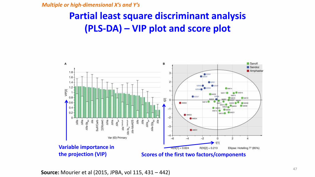
Partial least square discriminant analysis (PLS-DA) – VIP plot and score plot
47Source: Mourier et al (2015, JPBA, vol 115, 431 – 442)
Multiple or high-dimensional X’s and Y’s
Variable importance in the projection (VIP) Scores of the first two factors/components

Outline
• correlation analysis• linear regression• analysis of variance• contingency table analysis• logistic regression• ordinal logistic regression• survival analysis• discriminant analysis• cluster analysis• principal component analysis• partial least square discriminant analysis• three data sets
48

Three data sets (1)
• Data set 1 – A genetic data set with 2 SNPs
– Column 1: affection status
– Column 2: sex
– Column 3: Trait_1
– Column 4: SNP rs1318631 (0, 1, 2)
– Column 5: SNP rs2071591 (0, 1, 2)
49

Three data sets (2)
• Data set 2 – A gene expression data set from HapMap II
– Each row indicates a transcript (1,000 transcripts in total)
– Each column indicates a sample (210 samples in total; 60 CEUs, 60 YRIs, 45 CHBs, and 45 JPTs)
50
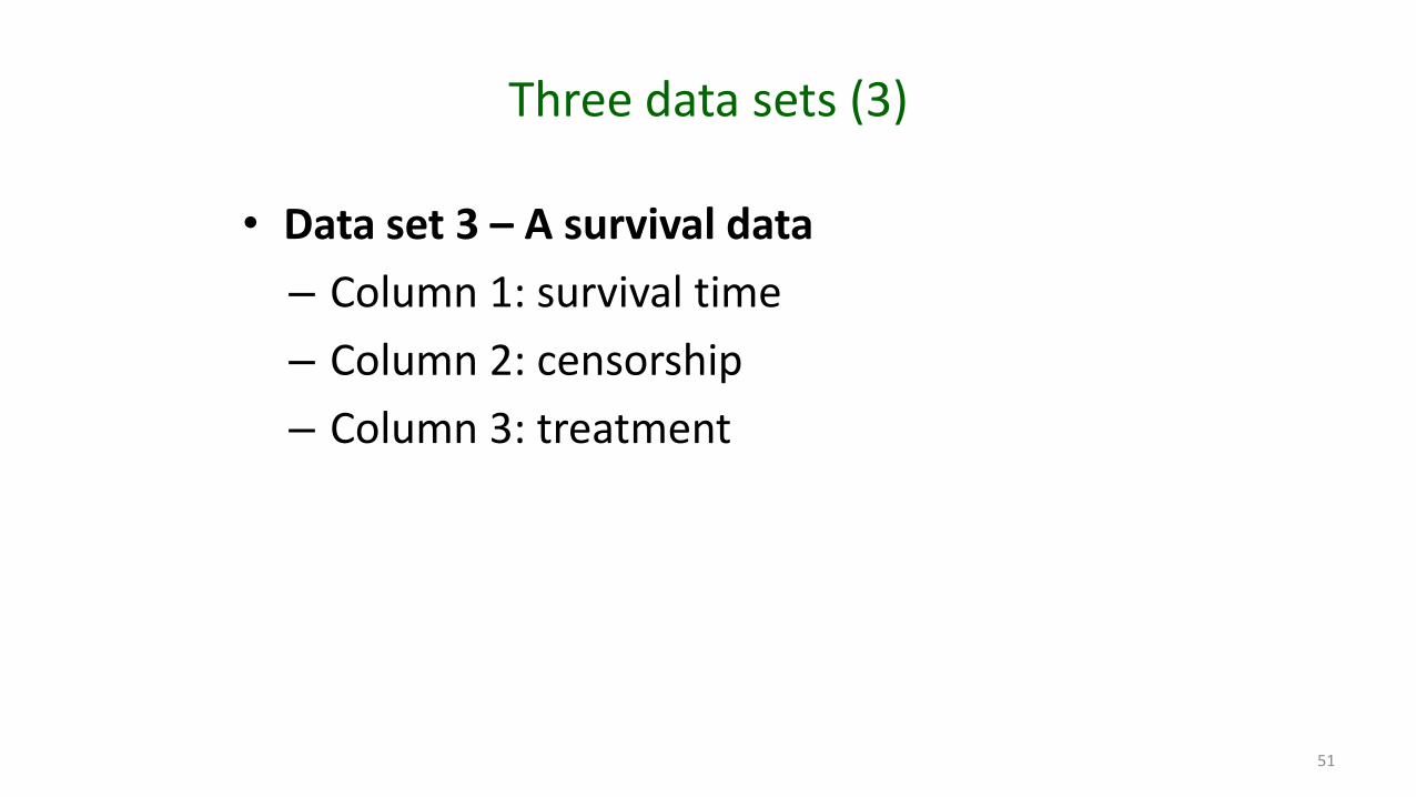
Three data sets (3)
• Data set 3 – A survival data
– Column 1: survival time
– Column 2: censorship
– Column 3: treatment
51

15:00 – 15:25Presenter: Yin-Chun Lin
15:25 – 15:50Presenter: Mei-Chu Huang
16:00 – 16:25Presenter: Jia-Wei Chen
16:25 – 16:50Presenter: Shih-Kai Chu
Take a break
Q & A

15:00 – 15:25Presenter: Yin-Chun Lin
15:25 – 15:50Presenter: Mei-Chu Huang
16:00 – 16:25Presenter: Jia-Wei Chen
16:25 – 16:50Presenter: Shih-Kai Chu
Take a break
Q & AProgram: Prog_1.r

Outline
• 1. Chi-square test
• 2. Fisher exact test
• 3. Logistic regression
• 4. Ordinal Logistic regression

Data description
• 800 patients and 800 controls.
• Column 1: 0: control; 1: patient.
• Column 2: F: Female; M: male.
• Column 3: trait score.
• Column 4: The coding 0, 1, 2 represent the number of minor allele for snp1 rs1318631.
• Column 5: The coding 0, 1, 2 represent the number of minor allele for snp2 rs2071591.
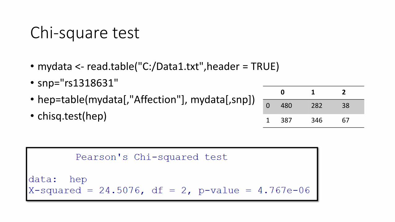
Chi-square test
• mydata <- read.table("C:/Data1.txt",header = TRUE)
• snp="rs1318631"
• hep=table(mydata[,"Affection"], mydata[,snp])
• chisq.test(hep)
0 1 2
0 480 282 38
1 387 346 67

Fisher exact test(Association between HLA and Stevens-Johnson syndrome)
CBZ-SJS CBZ-tolerant
HLA alleleB*1502
Yes 44 3
No 0 98
ta=matrix(c(44,0,3,98),nrow=2)fisher.test(ta)$p.value
#[1] 5.048442e-34
*In their paper, the p-value=3.13 × 10⁻²⁷ is calculated by Chi-square test with Bonferroni correction.
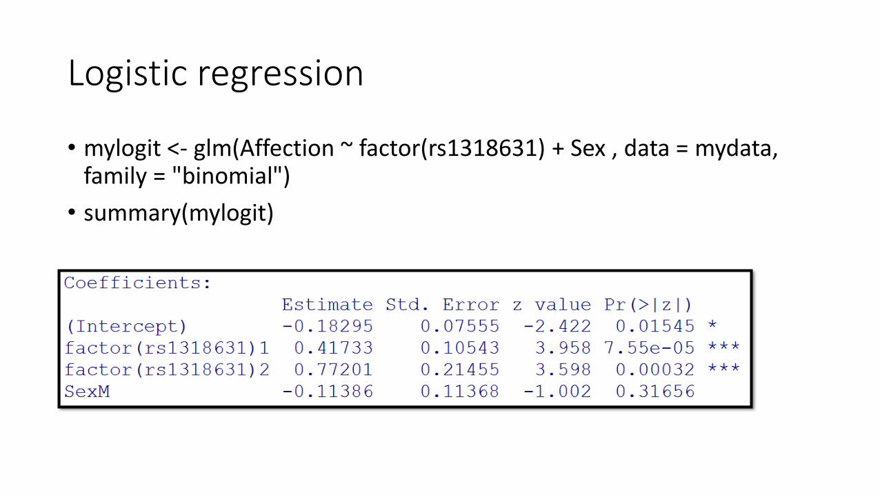
Logistic regression
• mylogit <- glm(Affection ~ factor(rs1318631) + Sex , data = mydata, family = "binomial")
• summary(mylogit)

• hep=table(mydata[,"Affection"], mydata[,snp])
• hep_prop=apply(hep,2,function(x) x/(sum(x)))
• barplot(hep_prop,xlab="Number of minor allele",ylab="Proportion")
0 1 2
0 0.57(0.55)
0.47(0.44)
0.4(0.35)
1 0.43(0.45)
0.53(0.56)
0.6(0.65)
M F

Ordinal Logistic regression
• library(VGAM)
• coding=function(x){#code trait1 to a categorical variable• temp=rep(1,length(x))• temp[x<250]=0• temp[x>500]=2• return(temp) }
• snp="rs2071591"
• x= factor(mydata[,snp])
• ccp=factor(coding(as.numeric(mydata[,"Trait_1"])),levels=c("0","1","2"),ordered=T)
• Sex= mydata$Sex
• ol=vglm(ccp ~ x +Sex ,family=propodds)
• p=attributes(summary(ol))$coef3

• log𝑝1
𝑝2+𝑝3= 𝛽10 + 𝛽1𝑆𝑁𝑃1,𝑟𝑒𝑓=0 + 𝛽2𝑆𝑁𝑃2,𝑟𝑒𝑓=0 + 𝛽3𝑆𝑒𝑥 + 𝑒
• log𝑝1+𝑝2
𝑝3= 𝛽20 + 𝛽1𝑆𝑁𝑃1,𝑟𝑒𝑓=0 + 𝛽2𝑆𝑁𝑃2,𝑟𝑒𝑓=0 + 𝛽3𝑆𝑒𝑥 + 𝑒

Any questions?

16:00 – 16:25Presenter: Jia-Wei Chen
16:25 – 16:50Presenter: Shih-Kai Chu
Take a break
Q & A
15:25 – 15:50Presenter: Mei-Chu Huang
15:00 – 15:25Presenter: Yin-Chun Lin
Program: Prog_2.r

Correlation, linear regression and ANOVA

Linear regression: data
• Data source: 1000 transcripts x 210 samples
Transcript ID
Transcript with rank 1 –log(P) value
Transcript with rank 2 –log(P) value
...
Transcript with rank 1000 –log(P) value
Sample ID
60 CEUs 60 YRIs 45 CHBs 45 JPTs
... ... ... ...
Linear regression: example 1
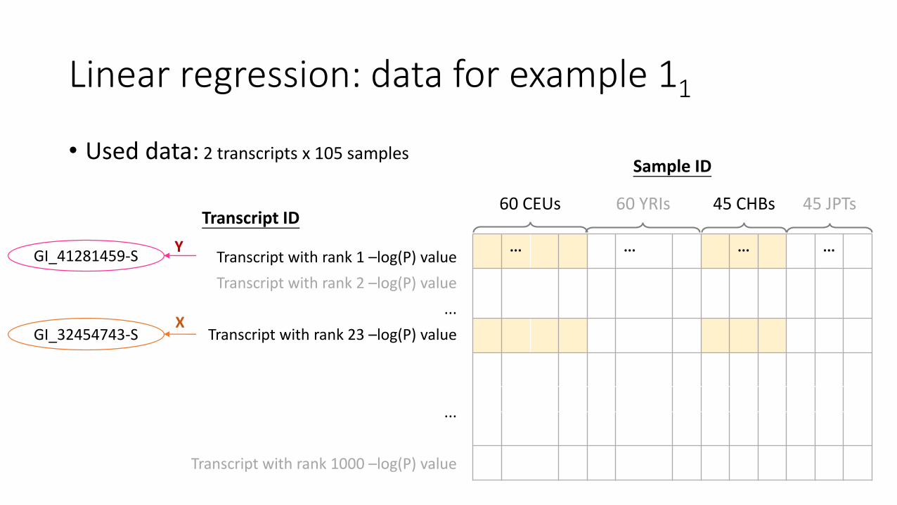
Linear regression: data for example 11
• Used data: 2 transcripts x 105 samples
... ... ... ...
Transcript ID
Transcript with rank 1 –log(P) value
Transcript with rank 2 –log(P) value
...
Transcript with rank 23 –log(P) value
...
Transcript with rank 1000 –log(P) value
Sample ID
60 CEUs 60 YRIs 45 CHBs 45 JPTs
GI_41281459-S
GI_32454743-S
Y
X

Linear regression: data for example 12
• Used data:
60 CEUs
45 CHBs
(GI_41281459-S)
Y
60 CEUs
45 CHBs
(GI_32454743-S)
X

Linear regression1data = as.matrix(read.table("C:/Data2.txt", header=T, sep="\t", as.is=T))
pp_popu = c(1:60, 121:165) # Select 60 CEU and 45 CHB samples
TSCP1 = "GI_41281459-S"; # Select the transcript as Y
Y = data[which(rownames(data)==TSCP1), pp_popu]
TSCP2 = "GI_32454743-S"; # Select the transcript as X
X = data[which(rownames(data)==TSCP2), pp_popu]
plot(X, Y, xlab=TSCP1, ylab=TSCP2, main="Gene expression data") # Scatter plot
lm_yx = lm(Y ~ X) # Fits a linear model Y ~ X to data
coryx = cor(X, Y, use = "complete.obs") # Calculate Pearson’s correlation ("pearson" (default), "kendall", or "spearman")
abline(lm_yx, col="red", lwd=2) # Add fit line
text(par("usr")[1], par("usr")[3]*1.01, paste("Cor = ", round(coryx, 3), sep=""), cex=1.25, col="blue", pos=4)# Add the correlation info to the plot

Linear regression2
Call:lm(formula = Y ~ X)
Residuals:Min 1Q Median 3Q Max
-0.90420 -0.32316 -0.03631 0.33069 0.81523
Coefficients:Estimate Std. Error t value Pr(>|t|)
(Intercept) 10.8739 1.2795 8.499 1.57e-13 ***X -0.1090 0.1431 -0.761 0.448 ---Signif. codes: 0 ‘***’ 0.001 ‘**’ 0.01 ‘*’ 0.05 ‘.’ 0.1 ‘ ’ 1
Residual standard error: 0.4028 on 103 degrees of freedomMultiple R-squared: 0.005595, Adjusted R-squared: -0.004059 F-statistic: 0.5795 on 1 and 103 DF, p-value: 0.4482
lm_yx = lm(Y ~ X) # Fits a linear model Y ~ X to data
summary(lm_yx) # Show summary statistics of the fitted linear model
−0.075 2
= 0.0056

Linear regression - considering interaction term1
• Used data:
60 CEUs
45 CHBs
(GI_41281459-S)
Y
60 CEUs
45 CHBs
(GI_32454743-S)
X
60 CEUs
45 CHBs
Popu
1
...
1
0
...
0
ቊCEU: 𝑝𝑜𝑝𝑢 = 1CHB: 𝑝𝑜𝑝𝑢 = 0

Linear regression - considering interaction term2
Call:lm(formula = Y ~ X + Popu + X * Popu)
Residuals:Min 1Q Median 3Q Max
-0.58275 -0.13527 0.01128 0.13760 0.50940
Coefficients:Estimate Std. Error t value Pr(>|t|)
(Intercept) 5.7474 1.0831 5.307 6.63e-07 ***X 0.5131 0.1223 4.197 5.83e-05 ***Popu 3.5278 1.3632 2.588 0.01108 * X:Popu -0.4762 0.1530 -3.112 0.00242 ** ---Signif. codes: 0 ‘***’ 0.001 ‘**’ 0.01 ‘*’ 0.05 ‘.’ 0.1 ‘ ’ 1
Residual standard error: 0.2004 on 101 degrees of freedomMultiple R-squared: 0.7586, Adjusted R-squared: 0.7514 F-statistic: 105.8 on 3 and 101 DF, p-value: < 2.2e-16
Popu = c(rep(1, 60), rep(0, 45)) # Set an indicator variable representing the population of transcripts
lm_yxp = lm(Y ~ X + Popu + X*Popu) # Fits a linear model with interaction term
summary(lm_yxp) # Show summary statistics of the fitted linear model
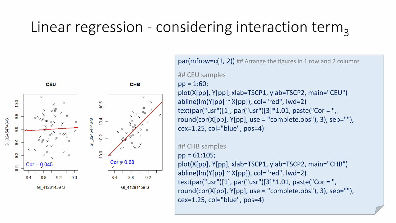
Linear regression - considering interaction term3
par(mfrow=c(1, 2)) ## Arrange the figures in 1 row and 2 columns
## CEU samplespp = 1:60;plot(X[pp], Y[pp], xlab=TSCP1, ylab=TSCP2, main="CEU")abline(lm(Y[pp] ~ X[pp]), col="red", lwd=2)text(par("usr")[1], par("usr")[3]*1.01, paste("Cor = ", round(cor(X[pp], Y[pp], use = "complete.obs"), 3), sep=""), cex=1.25, col="blue", pos=4)
## CHB samples pp = 61:105;plot(X[pp], Y[pp], xlab=TSCP1, ylab=TSCP2, main="CHB")abline(lm(Y[pp] ~ X[pp]), col="red", lwd=2)text(par("usr")[1], par("usr")[3]*1.01, paste("Cor = ", round(cor(X[pp], Y[pp], use = "complete.obs"), 3), sep=""), cex=1.25, col="blue", pos=4)

Linear regression: example 2
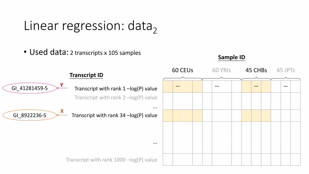
Linear regression: data2
• Used data: 2 transcripts x 105 samples
... ... ... ...
Transcript ID
Transcript with rank 1 –log(P) value
Transcript with rank 2 –log(P) value
...
Transcript with rank 34 –log(P) value
...
Transcript with rank 1000 –log(P) value
Sample ID
60 CEUs 60 YRIs 45 CHBs 45 JPTs
GI_41281459-S
GI_8922236-S
Y
X

Linear regression: data3
• Used data:
60 CEUs
45 CHBs
(GI_41281459-S)
Y
60 CEUs
45 CHBs
(GI_8922236-S)
X
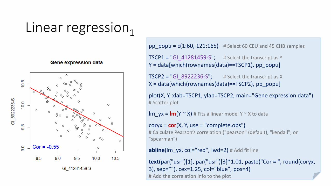
Linear regression1pp_popu = c(1:60, 121:165) # Select 60 CEU and 45 CHB samples
TSCP1 = "GI_41281459-S"; # Select the transcript as Y
Y = data[which(rownames(data)==TSCP1), pp_popu]
TSCP2 = "GI_8922236-S"; # Select the transcript as X
X = data[which(rownames(data)==TSCP2), pp_popu]
plot(X, Y, xlab=TSCP1, ylab=TSCP2, main="Gene expression data") # Scatter plot
lm_yx = lm(Y ~ X) # Fits a linear model Y ~ X to data
coryx = cor(X, Y, use = "complete.obs") # Calculate Pearson’s correlation ("pearson" (default), "kendall", or "spearman")
abline(lm_yx, col="red", lwd=2) # Add fit line
text(par("usr")[1], par("usr")[3]*1.01, paste("Cor = ", round(coryx, 3), sep=""), cex=1.25, col="blue", pos=4)# Add the correlation info to the plot

Linear regression2
Call:lm(formula = Y ~ X)
Residuals:Min 1Q Median 3Q Max
-0.74097 -0.23889 -0.03131 0.19221 0.72851
Coefficients:Estimate Std. Error t value Pr(>|t|)
(Intercept) 14.27822 0.65647 21.750 < 2e-16 ***X -0.46712 0.06996 -6.677 1.26e-09 ***---Signif. codes: 0 ‘***’ 0.001 ‘**’ 0.01 ‘*’ 0.05 ‘.’ 0.1 ‘ ’ 1
Residual standard error: 0.3374 on 103 degrees of freedomMultiple R-squared: 0.3021, Adjusted R-squared: 0.2953 F-statistic: 44.59 on 1 and 103 DF, p-value: 1.261e-09
lm_yx = lm(Y ~ X) # Fits a linear model Y ~ X to data
summary(lm_yx) # Show summary statistics of the fitted linear model
−0.55 2
= 0.3025

Linear regression - considering interaction term1
• Used data:
60 CEUs
45 CHBs
(GI_41281459-S)
Y
60 CEUs
45 CHBs
(GI_8922236-S)
X
60 CEUs
45 CHBs
Popu
1
...
1
0
...
0
ቊCEU: 𝑝𝑜𝑝𝑢 = 1CHB: 𝑝𝑜𝑝𝑢 = 0

Linear regression - considering interaction term2
Call:lm(formula = Y ~ X + Popu + X * Popu)
Residuals:Min 1Q Median 3Q Max
-0.50152 -0.14548 0.01239 0.15281 0.55649
Coefficients:Estimate Std. Error t value Pr(>|t|)
(Intercept) 8.11541 0.78770 10.303 < 2e-16 ***X 0.24065 0.08706 2.764 0.006784 ** Popu 3.50896 1.00885 3.478 0.000746 ***X:Popu -0.45034 0.10893 -4.134 7.37e-05 ***---Signif. codes: 0 ‘***’ 0.001 ‘**’ 0.01 ‘*’ 0.05 ‘.’ 0.1 ‘ ’ 1
Residual standard error: 0.2003 on 101 degrees of freedomMultiple R-squared: 0.7588, Adjusted R-squared: 0.7517 F-statistic: 105.9 on 3 and 101 DF, p-value: < 2.2e-16
Popu = c(rep(1, 60), rep(0, 45)) # Set an indicator variable representing the population of transcripts
lm_yxp = lm(Y ~ X + Popu + X*Popu) # Fits a linear model with interaction term
summary(lm_yxp) # Show summary statistics of the fitted linear model
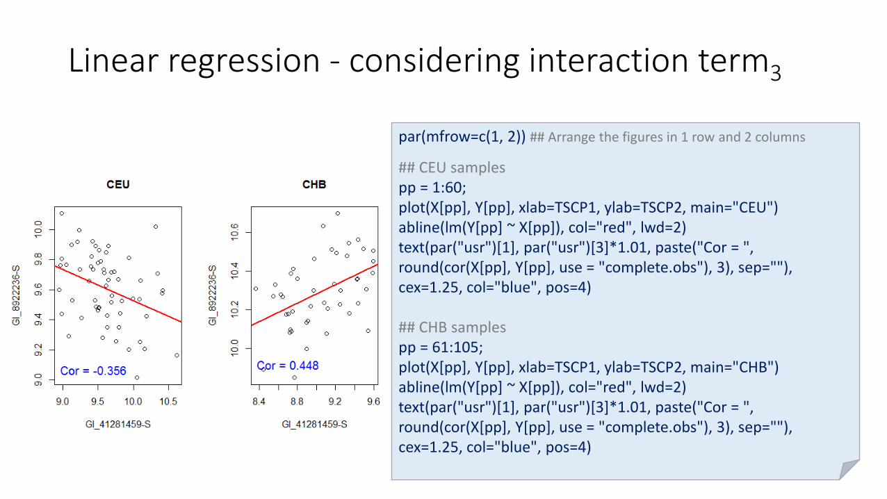
Linear regression - considering interaction term3
par(mfrow=c(1, 2)) ## Arrange the figures in 1 row and 2 columns
## CEU samplespp = 1:60;plot(X[pp], Y[pp], xlab=TSCP1, ylab=TSCP2, main="CEU")abline(lm(Y[pp] ~ X[pp]), col="red", lwd=2)text(par("usr")[1], par("usr")[3]*1.01, paste("Cor = ", round(cor(X[pp], Y[pp], use = "complete.obs"), 3), sep=""), cex=1.25, col="blue", pos=4)
## CHB samples pp = 61:105;plot(X[pp], Y[pp], xlab=TSCP1, ylab=TSCP2, main="CHB")abline(lm(Y[pp] ~ X[pp]), col="red", lwd=2)text(par("usr")[1], par("usr")[3]*1.01, paste("Cor = ", round(cor(X[pp], Y[pp], use = "complete.obs"), 3), sep=""), cex=1.25, col="blue", pos=4)

ANOVA: example 3

ANOVA: data1
• Used data: 1 transcripts x 210 samples
... ... ... ...
Transcript ID
Transcript with rank 1 –log(P) value
Transcript with rank 2 –log(P) value
...
...
Transcript with rank 1000 –log(P) value
Sample ID
60 CEUs 60 YRIs 45 CHBs 45 JPTs
GI_41281459-SY

ANOVA: data2
• Used data:
60 CEUs
45 CHBs
(GI_41281459-S)
Y PopuCEU: 𝑃𝑜𝑝𝑢 = 1YRI: 𝑃𝑜𝑝𝑢 = 2CHB: 𝑃𝑜𝑝𝑢 = 3𝐽𝑃𝑇: 𝑃𝑜𝑝𝑢 = 4
60 YRIs
45 JPTs
60 CEUs
45 CHBs
1
...
1
2
...
2
3...3
4...4
60 YRIs
45 JPTs
1
...
1
2
...
2
3...3
4...4

ANOVA: test 𝐻0: 𝜇𝐶𝐸𝑈 = 𝜇𝑌𝑅𝐼 = 𝜇𝐶𝐻𝐵 = 𝜇𝐽𝑃𝑇
Analysis of Variance Table
Response: YDf Sum Sq Mean Sq F value Pr(>F)
Popu 1 2.448 2.44801 20.157 1.181e-05 ***Residuals 208 25.261 0.12145 ---Signif. codes: 0 ‘***’ 0.001 ‘**’ 0.01 ‘*’ 0.05 ‘.’ 0.1 ‘ ’ 1
Y = data[which(rownames(data)==TSCP1), ]
Popu = c(rep(1, 60), rep(2, 60), rep(3, 45), rep(4, 45))# Set a variable representing the population of the transcript
anova(lm(Y ~ Popu)) # ANOVA

ANOVA: test 𝐻0: 𝜇𝑌𝑅𝐼 = 𝜇𝐶𝐻𝐵
Analysis of Variance Table
Response: YDf Sum Sq Mean Sq F value Pr(>F)
Popu 1 0.0165 0.016459 0.3906 0.5334Residuals 103 4.3405 0.042141
pp_popu = 61:165 # Select 60 YRI and 45 CHB samples
Y = data[which(rownames(data)==TSCP1), pp_popu]
Popu = c(rep(1, 60), rep(2, 45))# Set a variable representing the population of the transcript
anova(lm(Y ~ Popu)) # ANOVA

Survival analysis
CRAN Task View: Survival Analysis• Presents the useful R packages for the analysis of time to event data
• https://cran.r-project.org/web/views/Survival.html
• Version: 2016-05-26
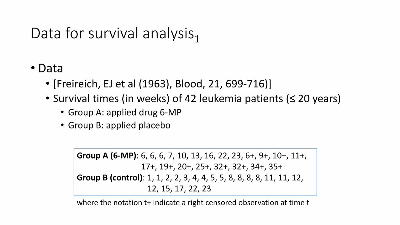
Data for survival analysis1
• Data• [Freireich, EJ et al (1963), Blood, 21, 699-716)]
• Survival times (in weeks) of 42 leukemia patients (≤ 20 years)• Group A: applied drug 6-MP
• Group B: applied placebo
Group A (6-MP): 6, 6, 6, 7, 10, 13, 16, 22, 23, 6+, 9+, 10+, 11+, 17+, 19+, 20+, 25+, 32+, 32+, 34+, 35+
Group B (control): 1, 1, 2, 2, 3, 4, 4, 5, 5, 8, 8, 8, 8, 11, 11, 12, 12, 15, 17, 22, 23
where the notation t+ indicate a right censored observation at time t

Data for survival analysis2
Status = 0: incomplete observation
cases
ctrls
Time Status Treatment
6 6 1 6-MP
6 6 1 6-MP
6 6 1 6-MP
6+ 6 0 6-MP
7 7 1 6-MP
9+ 9 0 6-MP
(not shown)
35+ 35 0 6-MP
1 1 1 Placebo
1 1 1 Placebo
2 2 1 Placebo
(not shown)
23 23 1 Placebo
• Example data: Data3.txt
data = read.table("C:/Data3.txt", header=T, sep="\t", as.is=T)
cased = data[data[, "Treatment"]=="6-MP", ]
# Focused on case samples
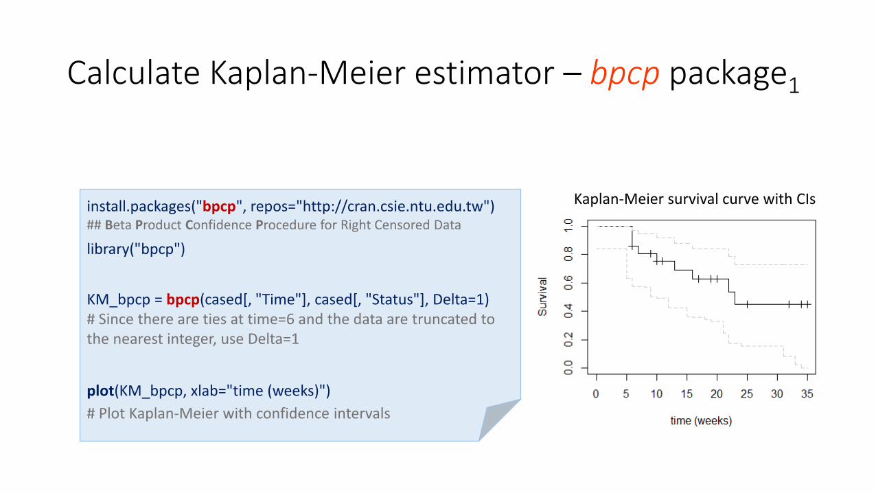
Calculate Kaplan-Meier estimator – bpcp package1
install.packages("bpcp", repos="http://cran.csie.ntu.edu.tw") ## Beta Product Confidence Procedure for Right Censored Data
library("bpcp")
KM_bpcp = bpcp(cased[, "Time"], cased[, "Status"], Delta=1)# Since there are ties at time=6 and the data are truncated to the nearest integer, use Delta=1
plot(KM_bpcp, xlab="time (weeks)")
# Plot Kaplan-Meier with confidence intervals
Kaplan-Meier survival curve with CIs

Calculate Kaplan-Meier estimator – bpcp package2
plot(KM_bpcp, xlab="time (weeks)")
# plot Kaplan-Meier with confidence intervals
lines(KM_bpcp, lwd=2, lty=c(2, 1, 2), col=c("skyblue", "navy",
"skyblue"))
## Modify the line styles to make the plot more clear
Kaplan-Meier survival curve with CIs

Survival probability (estimated using bpcp package)
time interval survival lower 95% CL upper 95% CL1 [0,5) 1.0000000 0.83890238 1.00000002 [5,6) 1.0000000 0.63177409 1.00000003 [6,7) 0.8571429 0.57230435 0.96951104 [7,8) 0.8067227 0.57230435 0.94482145 [8,9) 0.8067227 0.56700105 0.94482146 [9,10) 0.8067227 0.50082589 0.94482147 [10,11) 0.7529412 0.49364913 0.91503088 [11,12) 0.7529412 0.49364913 0.91503089 [12,13) 0.7529412 0.42655122 0.915030810 [13,15) 0.6901961 0.42655122 0.878901411 [15,16) 0.6901961 0.36436287 0.878901412 [16,17) 0.6274510 0.35572351 0.838416913 [17,18) 0.6274510 0.35572351 0.838416914 [18,19) 0.6274510 0.34482742 0.838416915 [19,20) 0.6274510 0.33079464 0.838416916 [20,21) 0.6274510 0.33079464 0.838416917 [21,22) 0.6274510 0.24813979 0.838416918 [22,23) 0.5378151 0.17619681 0.786465219 [23,24) 0.4481793 0.17619681 0.726063720 [24,25) 0.4481793 0.15704475 0.726063721 [25,31) 0.4481793 0.15704475 0.726063722 [31,32) 0.4481793 0.08445217 0.726063723 [32,33) 0.4481793 0.08445217 0.726063724 [33,34) 0.4481793 0.02337606 0.726063725 [34,35) 0.4481793 0.00000000 0.726063726 [35,Inf) 0.4481793 0.00000000 0.7260637
summary(KM_bpcp)
The calculation procedure is listed in the next slides
S 6 = Pr T > 6 =18
21= 0.8571429
S 7 = Pr T > 7 | T ≥ 7 ∙ Pr 𝑇 > 6
=16
17∙18
21= 0.8067227

Life table using the Kaplan-Meier approach
Time interval𝑡
𝑊𝑡 cAt risk Deaths during interval Survival probability
𝑁𝑡 b 𝑁𝑡 D 𝑊𝑡 D 𝑆𝑡+1 = 𝑆𝑡 ∙ ((𝑁𝑡+1 b − 𝑁𝑡+1 D )/𝑁𝑡+1 b )
[0,5) 21 021−0
21= 1
[5,6) (unchanged)
[6,7) 21 3 6, 6, 6 (21
21) ∙
21−3
21= 0.8571429
[7,8) 6+ 17 1 7 (21
21∙21−3
21) ∙
17−1
17= 0.8067227
[8,9) or [9,10) (unchanged)
[10,11) 9+ 15 1 10 (21
21∙21−3
21∙17−1
17) ∙
15−1
15= 0.7529412
[11,12) or [12,13) (unchanged)
[13,15) 10+, 11+ 12 1 13 (21
21∙21−3
21∙17−1
17∙15−1
15) ∙
12−1
12=0.6901961
... (not shown)
• 𝑡: Time interval• 𝑊𝑡 c : Survival time (in weeks) of censored samples at 𝑡• 𝑁𝑡 b : N of alive samples at beginning of time interval 𝑡• 𝑁𝑡 D : Number of deaths during time interval 𝑡• 𝑊𝑡 D : Survival time (in weeks) of deaths during time interval 𝑡

Calculate Kaplan-Meier estimator – survival package1
install.packages("survival", repos="http://cran.csie.ntu.edu.tw")
library("survival")
cased[, "SurvObj"] = Surv(cased[, "Time"], cased[, "Status"])
# Create a survival object (eg. 6+, 9+)
head(cased)
> head(cased)Time Status Treatment SurvObj
1 6 1 6-MP 6 2 6 1 6-MP 6 3 6 1 6-MP 6 4 6 0 6-MP 6+5 7 1 6-MP 7 6 9 0 6-MP 9+
Calculate Kaplan-Meier estimator – survival package2
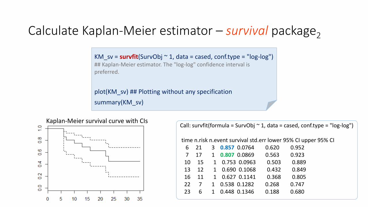
KM_sv = survfit(SurvObj ~ 1, data = cased, conf.type = "log-log") ## Kaplan-Meier estimator. The "log-log" confidence interval is preferred.
plot(KM_sv) ## Plotting without any specification
summary(KM_sv)
Call: survfit(formula = SurvObj ~ 1, data = cased, conf.type = "log-log")
time n.risk n.event survival std.err lower 95% CI upper 95% CI6 21 3 0.857 0.0764 0.620 0.9527 17 1 0.807 0.0869 0.563 0.92310 15 1 0.753 0.0963 0.503 0.88913 12 1 0.690 0.1068 0.432 0.84916 11 1 0.627 0.1141 0.368 0.80522 7 1 0.538 0.1282 0.268 0.74723 6 1 0.448 0.1346 0.188 0.680
Kaplan-Meier survival curve with CIs

Cox proportional hazards regression model(estimated using survival package)
Call:coxph(formula = data[, "SurvObj"] ~ Treatment, data = data)
n= 42, number of events= 30
coef exp(coef) se(coef) z Pr(>|z|) TreatmentPlacebo 1.5721 4.8169 0.4124 3.812 0.000138 ***---Signif. codes: 0 ‘***’ 0.001 ‘**’ 0.01 ‘*’ 0.05 ‘.’ 0.1 ‘ ’ 1
exp(coef) exp(-coef) lower .95 upper .95TreatmentPlacebo 4.817 0.2076 2.147 10.81
Concordance= 0.69 (se = 0.053 )Rsquare= 0.322 (max possible= 0.988 )Likelihood ratio test= 16.35 on 1 df, p=5.261e-05Wald test = 14.53 on 1 df, p=0.0001378Score (logrank) test = 17.25 on 1 df, p=3.283e-05
data[, "SurvObj"] = Surv(data[, "Time"], data[, "Status"])# Generate a survival object (eg. 6+, 9+)
cox_model = coxph(data[, "SurvObj"] ~ Treatment, data=data)# Fits a Cox proportional hazards regression model
summary(cox_model) # Show fitted results

Any questions?

16:25 – 16:50Presenter: Shih-Kai Chu
Take a break
Q & A
15:00 – 15:25Presenter: Yin-Chun Lin
15:25 – 15:50Presenter: Mei-Chu Huang
16:00 – 16:25Presenter: Jia-Wei Chen
Program: Prog_3.r

Dataset 2
• Import data for exercise
> hapmap <- read.table ("Data2.txt" , sep = "\t" , header = T , stringsAsFactors = F )
> hapmap <- as.data.frame ( t ( hapmap ) ) # transpose data ( Sample х Variable )
> POPU <- c ("CEU" , "YRI", "CHB" , "JPT" )
> popu <- rep ( POPU , c ( 60 , 60 , 45 , 45 ) )
210 samples
60 CEUs 60 YRIs 45 CHBs 45 JPTs
1,0
00
gen
e ex
pre
ssio
ns
1,000 gene expressions
21
0 s
amp
les
60 C
EUs
60 Y
RIs
45
CH
Bs
45 J
PTs
100
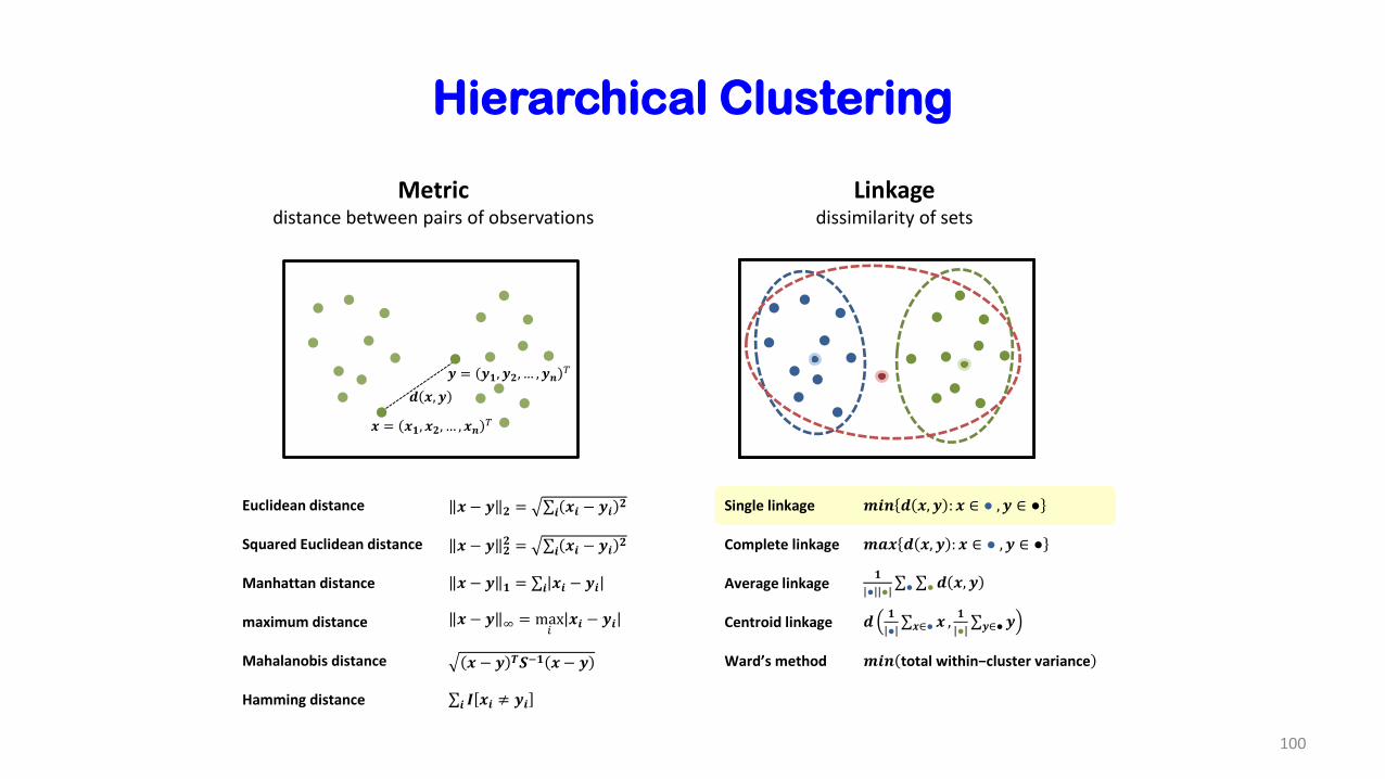
Hierarchical Clustering
Metricdistance between pairs of observations
Linkagedissimilarity of sets
Euclidean distance 𝒙 − 𝒚 𝟐 = σ𝒊 𝒙𝒊 − 𝒚𝒊𝟐
Squared Euclidean distance 𝒙 − 𝒚 𝟐𝟐 = σ𝒊 𝒙𝒊 − 𝒚𝒊
𝟐
Manhattan distance 𝒙 − 𝒚 𝟏 = σ𝒊 𝒙𝒊 − 𝒚𝒊
maximum distance 𝒙 − 𝒚 ∞ = max𝑖
𝒙𝒊 − 𝒚𝒊
Mahalanobis distance 𝒙 − 𝒚 𝑻𝑺−𝟏 𝒙 − 𝒚
Hamming distance σ𝒊 𝑰 𝒙𝒊 ≠ 𝒚𝒊
𝒙 = 𝒙𝟏, 𝒙𝟐, … , 𝒙𝒏𝑇
𝒚 = 𝒚𝟏, 𝒚𝟐, … , 𝒚𝒏𝑇
𝒅 𝒙, 𝒚
Single linkage 𝒎𝒊𝒏 𝒅 𝒙, 𝒚 : 𝒙 ∈ ● , 𝒚 ∈ ●
Complete linkage 𝒎𝒂𝒙 𝒅 𝒙, 𝒚 : 𝒙 ∈ ● , 𝒚 ∈ ●
Average linkage𝟏
● ●σ●σ●𝒅 𝒙, 𝒚
Centroid linkage 𝒅𝟏
●σ𝒙∈●𝒙 ,
𝟏
●σ𝒚∈●𝒚
Ward’s method 𝒎𝒊𝒏 total within−cluster variance

101
Hierarchical Clustering
• Using dist() {stats} to calculate distance between pairs of samples
> hapmap.dist <- dist ( hapmap , method = "euclidean" ) # calculate distance between pairs of samples
• Using hclust() {stats} to conduct a clustering analysis
> hapmap.cl_a <- hclust ( hapmap.dist , method = "average" ) # average-linkage clustering
• Using plot() to visualize clustering result
> COL <- 1 : 4; names ( COL ) <- POPU
> plot ( hapmap.cl_a , hang = -1 , main = "HapMapII" , cex = .5 ) # visualization reference
CEUYRICHBJPT
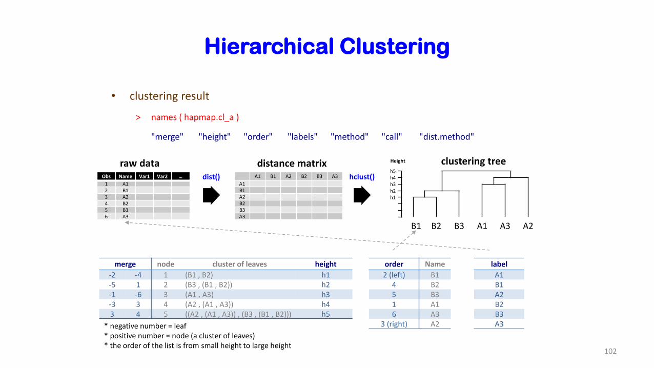
• clustering result
> names ( hapmap.cl_a )
"merge" "height" "order" "labels" "method" "call" "dist.method"
102
Hierarchical Clustering
Height clustering treeh5h4h3h2h1
B1 B2 B3 A1 A3 A2
Obs Name Var1 Var2 …
1 A12 B13 A24 B25 B36 A3
order Name
2 (left) B14 B25 B31 A16 A3
3 (right) A2
merge node cluster of leaves height
-2 -4 1 (B1 , B2) h1-5 1 2 (B3 , (B1 , B2)) h2-1 -6 3 (A1 , A3) h3-3 3 4 (A2 , (A1 , A3)) h43 4 5 ((A2 , (A1 , A3)) , (B3 , (B1 , B2))) h5
* negative number = leaf* positive number = node (a cluster of leaves)* the order of the list is from small height to large height
raw datadist() A1 B1 A2 B2 B3 A3
A1B1A2B2B3A3
hclust()
label
A1B1A2B2B3A3
distance matrix
103
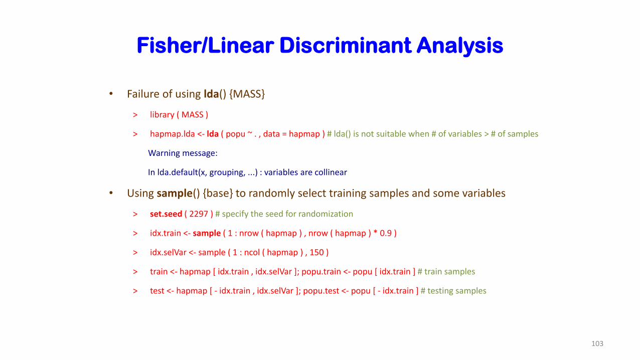
Fisher/Linear Discriminant Analysis
• Failure of using lda() {MASS}
> library ( MASS )
> hapmap.lda <- lda ( popu ~ . , data = hapmap ) # lda() is not suitable when # of variables > # of samples
Warning message:
In lda.default(x, grouping, ...) : variables are collinear
• Using sample() {base} to randomly select training samples and some variables
> set.seed ( 2297 ) # specify the seed for randomization
> idx.train <- sample ( 1 : nrow ( hapmap ) , nrow ( hapmap ) * 0.9 )
> idx.selVar <- sample ( 1 : ncol ( hapmap ) , 150 )
> train <- hapmap [ idx.train , idx.selVar ]; popu.train <- popu [ idx.train ] # train samples
> test <- hapmap [ - idx.train , idx.selVar ]; popu.test <- popu [ - idx.train ] # testing samples

104
Fisher/Linear Discriminant Analysis
• LDA for training data
> hapmap.lda <- lda ( popu.train ~ . , data = train )
• Using plot() to visualize LDA result
> plot ( hapmap.lda , panel = function ( x , y , ... ) { text ( x , y , popu.train , col = COL [ popu.train ] ) } )
CEUYRICHBJPT

105
Fisher/Linear Discriminant Analysis
• LDA result
> names ( hapmap.lda )
"prior" "counts" "means" "scaling" "lev" "svd" "N" "call" "terms" "xlevels"
1. group mean 𝒎𝒊 (means)
2. within-class scatter matrix 𝑺𝑾 = σ𝒙∈𝑪𝒊𝑺𝒊, where 𝑺𝒊 = σ𝒙∈𝑪𝒊
𝒙 −𝒎𝒊 𝒙 −𝒎𝒊𝑻
between-class scatter matrix 𝑺𝑩 = σ𝒊∈𝑪 𝒎𝒊 −𝒎 𝒎𝒊 −𝒎 𝑻 , where 𝒎 = σ𝒙∈𝑪𝒊𝒙 /𝒏
3. solve the generalized eigenvalue problem for 𝑺𝑩
𝑺𝒘to get
1) eigenvalues (svd)
2) 𝓵 eigenvectors with the largest eigenvalues to form a 𝒑 × 𝓵 matrix 𝑾 (scaling)
4. transform the samples onto the new subspace 𝒀′ = 𝑿𝑾𝑻
106
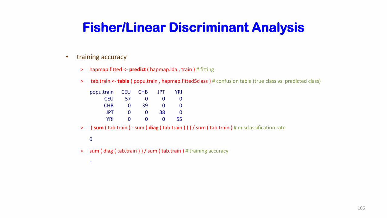
Fisher/Linear Discriminant Analysis
• training accuracy
> hapmap.fitted <- predict ( hapmap.lda , train ) # fitting
> tab.train <- table ( popu.train , hapmap.fitted$class ) # confusion table (true class vs. predicted class)
> ( sum ( tab.train ) - sum ( diag ( tab.train ) ) ) / sum ( tab.train ) # misclassification rate
0
> sum ( diag ( tab.train ) ) / sum ( tab.train ) # training accuracy
1
popu.train CEU CHB JPT YRICEU 57 0 0 0CHB 0 39 0 0JPT 0 0 38 0YRI 0 0 0 55

107
Fisher/Linear Discriminant Analysis
• prediction and testing accuracy
> hapmap.pred <- predict ( hapmap.lda , test )
> tab <- table ( popu.test , hapmap.pred$class ) # confusion table (true class vs. predicted class)
> sum ( tab [ upper.tri ( tab ) ] , tab [ lower.tri ( tab ) ] ) / sum ( tab ) # misclassification rate
0.1428571 # ( 1 + 2 ) / ( 3 + 5 + 1 + 2 + 5 + 5 )
> sum ( diag ( tab.test) ) / sum ( tab.test ) # testing accuracy
0.8571429 # ( 3 + 5 + 5 + 5 ) / ( 3 + 5 + 1 + 2 + 5 + 5 )
popu.test CEU CHB JPT YRICEU 3 0 0 0CHB 0 5 1 0JPT 0 2 5 0YRI 0 0 0 5

Any questions?

Take a break
15:00 – 15:25Presenter: Yin-Chun Lin
15:25 – 15:50Presenter: Mei-Chu Huang
16:00 – 16:25Presenter: Jia-Wei Chen
16:25 – 16:50Presenter: Shih-Kai Chu
Q & AProgram: Prog_4.r

Dimension ReductionPCA & PLS
Hands-on
Gene expression profilesin HapMap project
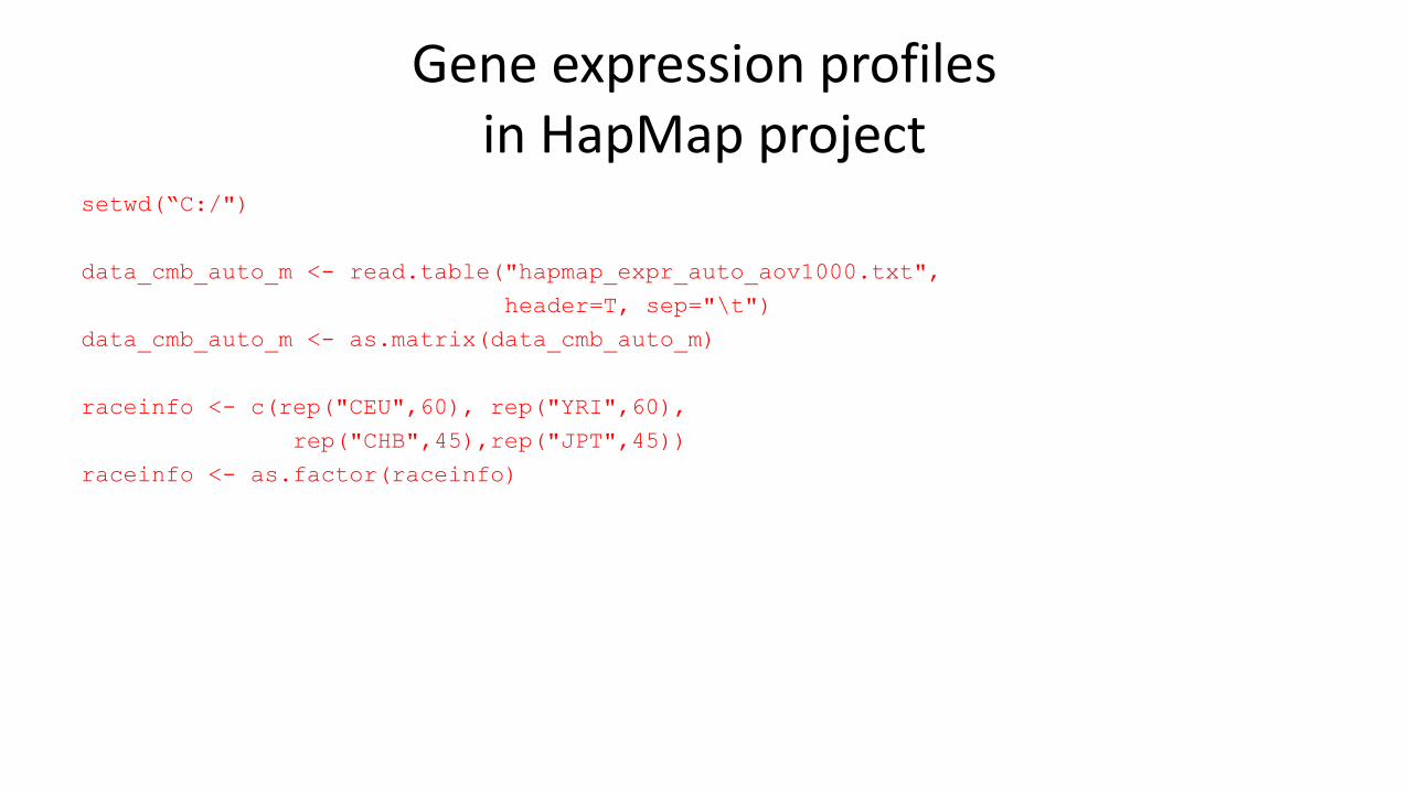
setwd(“C:/")
data_cmb_auto_m <- read.table("hapmap_expr_auto_aov1000.txt",
header=T, sep="\t")
data_cmb_auto_m <- as.matrix(data_cmb_auto_m)
raceinfo <- c(rep("CEU",60), rep("YRI",60),
rep("CHB",45),rep("JPT",45))
raceinfo <- as.factor(raceinfo)

PRINCIPAL COMPONENT ANALYSIS (PCA)

?prcomp
Reference: The R Book http://las.sinica.edu.tw/search*eng/i?SEARCH=9781118448908

Principal component analysis
pcafit <- prcomp(t(data_cmb_auto_m),scale=TRUE)
ls(pcafit)
plot(pcafit) ## scree plot
summary(pcafit,digits=2)$importance[,1:5]
pcafit$sdev[1:5]
pcafit$x[1:5,1:5]
pcafit$rotation[1:5,1:5]
𝑋 = 𝑈 𝐷 𝑉𝑇
(x) (sdev) (rotation)T
PCA as an exploratory tool
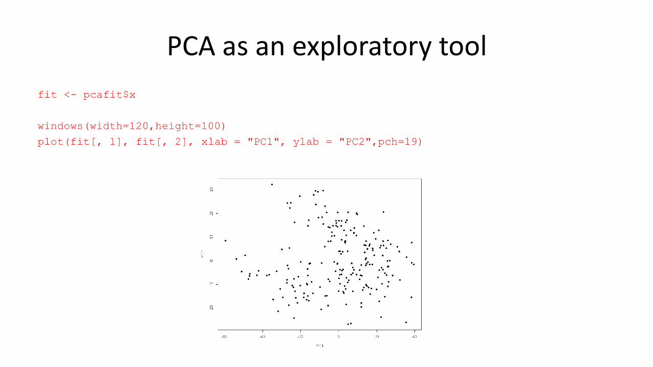
fit <- pcafit$x
windows(width=120,height=100)
plot(fit[, 1], fit[, 2], xlab = "PC1", ylab = "PC2",pch=19)

PCA as an exploratory tool (cont’d)
library(RColorBrewer)
pal = brewer.pal(9, "Set1")
col <- pal[raceinfo]
numGroups <-
length(levels(raceinfo))
windows(width=120,height=100)
plot(fit[,1],fit[,2], xlab ="PC1",
ylab ="PC2", col=col, pch=19)
legend("bottomright", legend =
levels(raceinfo),
ncol = numGroups, text.col
= pal[1:numGroups])
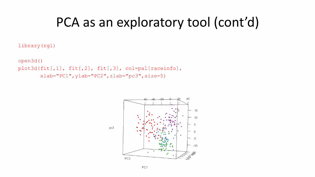
library(rgl)
open3d()
plot3d(fit[,1], fit[,2], fit[,3], col=pal[raceinfo],
xlab="PC1",ylab="PC2",zlab="pc3",size=5)
PCA as an exploratory tool (cont’d)

biplot(pcafit)
# biplot ( pca on 20 vars * 120 samples)
Further analysis using PCs
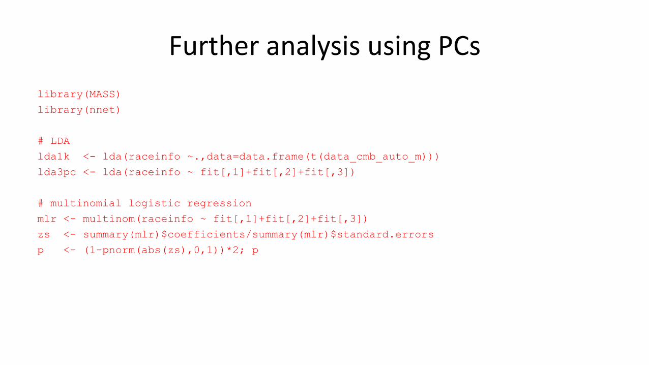
library(MASS)
library(nnet)
# LDA
lda1k <- lda(raceinfo ~.,data=data.frame(t(data_cmb_auto_m)))
lda3pc <- lda(raceinfo ~ fit[,1]+fit[,2]+fit[,3])
# multinomial logistic regression
mlr <- multinom(raceinfo ~ fit[,1]+fit[,2]+fit[,3])
zs <- summary(mlr)$coefficients/summary(mlr)$standard.errors
p <- (1-pnorm(abs(zs),0,1))*2; p

PARTIAL LEAST SQUARE DISCRIMINANT ANALYSIS (PLS-DA)

Gene expression profilesin HapMap project
# extract 50 CEUs and 50 YRIs
data_cmb_auto_mt <- data_cmb_auto_m[,c(1:50,61:110)]
raceinfo2 <- c(rep("CEU",50),rep("YRI",50))

Install ropls
## try http:// if https:// URLs are not supported
source("https://bioconductor.org/biocLite.R")
biocLite("ropls")
library(ropls)
?opls
Reference:S. Wold, M. Sjöström, L. ErikssonChemom. Intell. Lab. Syst., 58 (2001), pp. 109–130ropls documentation https://www.bioconductor.org/packages/release/bioc/vignettes/ropls/inst/doc/ropls.pdf

PLS discriminant analysis
plsfit <- opls(t(data_cmb_auto_mt),raceinfo2,plotL=FALSE)
plsfit@summaryDF
R2X(cum) R2Y(cum) Q2(cum) RMSEE pre ort pR2Y pQ2
Total 0.615 0.983 0.94 0.0674 4 0 0.05 0.05
plsfit@modelDF
R2X R2X(cum) R2Y R2Y(cum) Q2 Q2(cum) Signif. Iter.
p1 0.4830 0.483 0.7620 0.762 0.750 0.750 R1 1
p2 0.0868 0.569 0.1170 0.879 0.425 0.856 R1 1
p3 0.0296 0.599 0.0722 0.951 0.391 0.913 R1 1
p4 0.0163 0.615 0.0315 0.983 0.314 0.940 R1 1
# a new component h is added to the model if:
# (1) R2Yh≥1% ; (2) Q2Yh≥0

PLS discriminant analysis (cont’d)
layout(matrix(1:4, nrow = 2, byrow = TRUE))
for(typeC in c("permutation", "overview", "outlier", "x-score"))
plot(plsfit, typeVc = typeC, parDevNewL = FALSE)
head(plsfit@scoreMN); dim(plsfit@scoreMN)

Variable Influence on Projection
head(plsfit@vipVn)
VIP
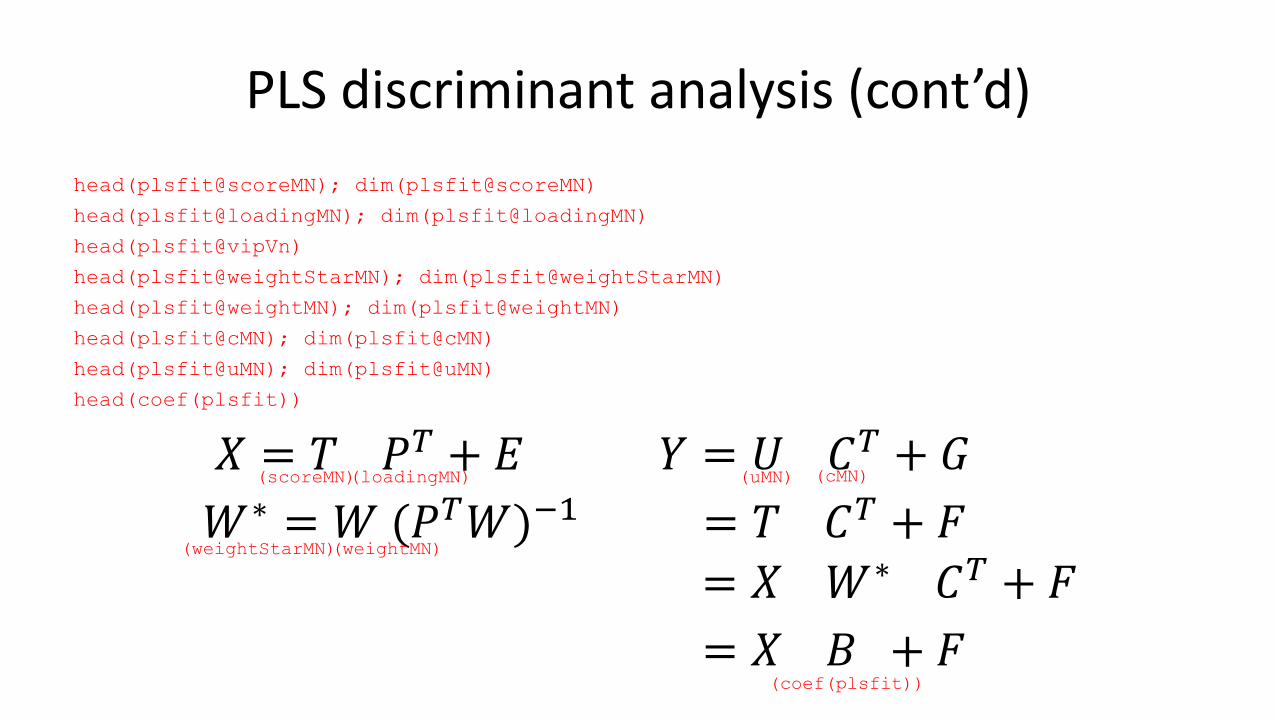
PLS discriminant analysis (cont’d)
head(plsfit@scoreMN); dim(plsfit@scoreMN)
head(plsfit@loadingMN); dim(plsfit@loadingMN)
head(plsfit@vipVn)
head(plsfit@weightStarMN); dim(plsfit@weightStarMN)
head(plsfit@weightMN); dim(plsfit@weightMN)
head(plsfit@cMN); dim(plsfit@cMN)
head(plsfit@uMN); dim(plsfit@uMN)
head(coef(plsfit))
𝑋 = 𝑇 𝑃𝑇 + 𝐸 𝑌 = 𝑈 𝐶𝑇 + 𝐺
= 𝑇 𝐶𝑇 + 𝐹
= 𝑋 𝑊∗ 𝐶𝑇 + 𝐹
= 𝑋 𝐵 + 𝐹
𝑊∗ = 𝑊 (𝑃𝑇𝑊)−1(scoreMN)(loadingMN)
(weightStarMN)(weightMN)
(uMN) (cMN)
(coef(plsfit))

Prediction by generated model
head(coef(plsfit))
table(raceinfo2, pls_fit=fitted(plsfit))
data_cmb_auto_mp <- data_cmb_auto_m[,c(51:60,111:120)]
table(c(rep("CEU",10),rep("YRI",10)),
predict(plsfit,t(data_cmb_auto_mp)))

Any questions?