Spatial Data Mining

Overview of Classification Techniques

2

Decision TreesTree-based classifiers for instances represented as feature-vectors. Nodes test features, there is one branch for each value of the feature, and leaves specify the category.

Can represent arbitrary conjunction and disjunction. Can represent any classification function over discrete feature vectors.Can be rewritten as a set of rules, i.e. disjunctive normal form (DNF).

red ∧ circle → posred ∧ circle → Ablue → B; red ∧ square → Bgreen → C; red ∧ triangle → C

color

red blue green

shape

circle square triangleneg pos

pos neg neg

color

red blue green

shape

circle square triangleB C

A B C

3

shape

circle square triangle

Top-Down Decision Tree InductionRecursively build a tree top-down by divide and conquer. <big, red, circle>: + <small, red, circle>: +

<small, red, square>: − <big, blue, circle>: −

<big, red, circle>: + <small, red, circle>: +<small, red, square>: −

color

red blue green

<big, red, circle>: + <small, red, circle>: +

pos<small, red, square>: −neg pos

<big, blue, circle>: −neg neg

4

Picking a Good Split Feature

Goal is to have the resulting tree be as small as possible, per Occam’s razor.Finding a minimal decision tree (nodes, leaves, or depth) is an NP-hard optimization problem.Top-down divide-and-conquer method does a greedy search for a simple tree but does not guarantee to find the smallest.

General lesson in ML: “Greed is good.”Want to pick a feature that creates subsets of examples that are relatively “pure” in a single class so they are “closer” to being leaf nodes.There are a variety of heuristics for picking a good test, a popular one is based on information gain that originated with the ID3 system of Quinlan (1979).

5

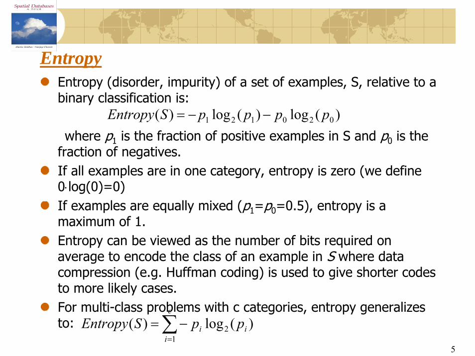
EntropyEntropy (disorder, impurity) of a set of examples, S, relative to a binary classification is:

where p1 is the fraction of positive examples in S and p0 is the fraction of negatives.If all examples are in one category, entropy is zero (we define 0⋅log(0)=0)If examples are equally mixed (p1=p0=0.5), entropy is a maximum of 1.Entropy can be viewed as the number of bits required on average to encode the class of an example in S where data compression (e.g. Huffman coding) is used to give shorter codes to more likely cases.For multi-class problems with c categories, entropy generalizes to:

)(log)(log)( 020121 ppppSEntropy −−=

∑−=c

ii ppSEntropy 2 )(log)(=i 1

6

Entropy Plot for Binary Classification

7

Information GainThe information gain of a feature F is the expected reduction in entropy resulting from splitting on this feature.

where Sv is the subset of S having value v for feature F.Entropy of each resulting subset weighted by its relative size.Example:

<big, red, circle>: + <small, red, circle>: +<small, red, square>: − <big, blue, circle>: −

)()(),()(

vFValuesv

v SEntropySS

SEntropyFSGain ∑∈

−=

2+, 2 −: E=1size

big small1+,1− 1+,1−E=1 E=1

Gain=1−(0.5⋅1 + 0.5⋅1) = 0

2+, 2 − : E=1color

red blue2+,1− 0+,1−E=0.918 E=0

Gain=1−(0.75⋅0.918 +0.25⋅0) = 0.311

2+, 2 − : E=1shape

circle square2+,1− 0+,1−E=0.918 E=0

Gain=1−(0.75⋅0.918 +0.25⋅0) = 0.311

8

History of Decision-Tree Research

Hunt and colleagues use exhaustive search decision-tree methods (CLS) to model human concept learning in the 1960’s.In the late 70’s, Quinlan developed ID3 with the information gain heuristic to learn expert systems from examples.Simulataneously, Breiman and Friedman and colleagues develop CART (Classification and Regression Trees), similar to ID3.In the 1980’s a variety of improvements are introduced to handle noise, continuous features, missing features, and improved splitting criteria. Various expert-system development tools results.Quinlan’s updated decision-tree package (C4.5) released in 1993.Weka includes Java version of C4.5 called J48.

9

Computational ComplexityWorst case builds a complete tree where every path test every feature. Assume n examples and mfeatures.

At each level, i, in the tree, must examine the remaining m− i features for each instance at the level to calculate info gains.

However, learned tree is rarely complete (number of leaves is ≤ n). In practice, complexity is linear in both number of features (m) and number of training examples (n).

F1

Fm

⋅⋅⋅⋅⋅ Maximum of n examples spread acrossall nodes at each of the m levels

)(1

2∑=

=⋅m

i

nmOni

10

OverfittingLearning a tree that classifies the training data perfectly may not lead to the tree with the best generalization to unseen data.

There may be noise in the training data that the tree is erroneously fitting.The algorithm may be making poor decisions towards the leaves of the tree that are based on very little data and may not reflect reliable trends.

A hypothesis, h, is said to overfit the training data is there exists another hypothesis which, h´, such that hhas less error than h´ on the training data but greater error on independent test data.

hypothesis complexity

accu

racy on training data

on test data

11

Overfitting Example

voltage (V)

curr

ent

(I)

Testing Ohms Law: V = IR (I = (1/R)V)

Ohm was wrong, we have found a more accurate function!

Perfect fit to training data with an 9th degree polynomial(can fit n points exactly with an n-1 degree polynomial)

Experimentallymeasure 10points

Fit a curve tothe resulting data.

12

Overfitting Example

voltage (V)

curr

ent

(I)

Testing Ohms Law: V = IR (I = (1/R)V)

Better generalization with a linear functionthat fits training data less accurately.

13

Overfitting Prevention (Pruning) MethodsTwo basic approaches for decision trees

Prepruning: Stop growing tree as some point during top-down construction when there is no longer sufficient data to make reliable decisions.Postpruning: Grow the full tree, then remove subtrees that do not have sufficient evidence.

Label leaf resulting from pruning with the majority class of the remaining data, or a class probability distribution. Method for determining which subtrees to prune:

Cross-validation: Reserve some training data as a hold-out set (validation set, tuning set) to evaluate utility of subtrees.Statistical test: Use a statistical test on the training data to determine if any observed regularity can be dismisses as likely due to random chance.Minimum description length (MDL): Determine if the additional complexity of the hypothesis is less complex than just explicitly remembering any exceptions resulting from pruning.

14

Neural Network Learning

Learning approach based on modeling adaptation in biological neural systems.Perceptron: Initial algorithm for learning simple neural networks (single layer) developed in the 1950’s.Backpropagation: More complex algorithm for learning multi-layer neural networks developed in the 1980’s.

15

Artificial Neuron ModelModel network as a graph with cells as nodes and synaptic connections as weighted edges from node ito node j, wji

Model net input to cell as

Cell output is:

1

32 54 6

w12

w13w14

w15w16

ii

jij ownet ∑=

(Tj is threshold for unit j)

ji

jjj Tnet

Tneto

≥<

= if 1 if 0

netj

oj

Tj0

1

16

Perceptron Learning AlgorithmIteratively update weights until convergence.

Each execution of the outer loop is typically called an epoch.

Initialize weights to random valuesUntil outputs of all training examples are correct

For each training pair, E, do: Compute current output oj for E given its inputsCompare current output to target value, tj , for EUpdate synaptic weights and threshold using learning rule

17

Perceptron Learning Rule

Update weights by:

where η is the “learning rate”tj is the teacher specified output for unit j.

Equivalent to rules:If output is correct do nothing.If output is high, lower weights on active inputsIf output is low, increase weights on active inputs

Also adjust threshold to compensate:

ijjjiji ootww )( −+= η

)( jjjj otTT −−= η

18

Concept Perceptron Cannot LearnCannot learn exclusive-or, or parity function in general.

o3

o2

??+1

01

–

+–

19

Perceptron Limits

System obviously cannot learn concepts it cannot represent.Minksy and Papert (1969) wrote a book analyzing the perceptron and demonstrating many functions it could not learn.These results discouraged further research on neural nets; and symbolic AI became the dominate paradigm.

20

Multi-Layer NetworksMulti-layer networks can represent arbitrary functions, but an effective learning algorithm for such networks was thought to be difficult.A typical multi-layer network consists of an input, hidden and output layer, each fully connected to the next, with activation feeding forward.

The weights determine the function computed. Given an arbitrary number of hidden units, any boolean function can be computed with a single hidden layer.

output

hidden

input

activation

21

Sample Learned XOR Network3.11

−7.386.96

−5.24

−3.6−3.58

−5.74

−2.03A

X Y

B

O

−5.57

Hidden Unit A represents: ¬(X ∧ Y)Hidden Unit B represents: ¬(X ∨ Y)Output O represents: A ∧ ¬B = ¬(X ∧ Y) ∧ (X ∨ Y)

= X ⊕ Y

22

Comments on Training AlgorithmNot guaranteed to converge to zero training error, may converge to local optima or oscillate indefinitely.However, in practice, does converge to low error for many large networks on real data.Many epochs (thousands) may be required, hours or days of training for large networks.To avoid local-minima problems, run several trials starting with different random weights (random restarts).

Take results of trial with lowest training set error.Build a committee of results from multiple trials (possibly weighting votes by training set accuracy).

23

Determining the Best Number of Hidden UnitsToo few hidden units prevents the network from adequately fitting the data.Too many hidden units can result in over-fitting.

Use internal cross-validation to empirically determine an optimal number of hidden units.

erro

r

on training data0 # hidden units

on test data

24

Successful Applications

Text to Speech (NetTalk)Fraud detectionFinancial Applications

HNC (eventually bought by Fair Isaac)Chemical Plant Control

Pavillion TechnologiesAutomated VehiclesGame Playing

NeurogammonHandwriting recognition

25

Issues in Neural Nets

More efficient training methods:QuickpropConjugate gradient (exploits 2nd derivative)

Learning the proper network architecture:Grow network until able to fit data

• Cascade Correlation• Upstart

Shrink large network until unable to fit data• Optimal Brain Damage

Recurrent networks that use feedback and can learn finite state machines with “backpropagation through time.”

Linear SeparatorsWhich of the linear separators is optimal?

Classification MarginDistance from example xi to the separator is Examples closest to the hyperplane are support vectors. Margin ρ of the separator is the distance between support vectors.

wxw br iT +

=

r

ρ

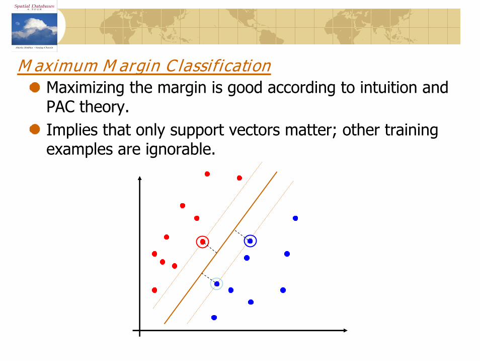
M aximum M argin C lassificationMaximizing the margin is good according to intuition and PAC theory.Implies that only support vectors matter; other training examples are ignorable.

Soft Margin Classification

What if the training set is not linearly separable?Slack variables ξi can be added to allow misclassification of difficult or noisy examples, resulting margin called soft.

ξi

ξi

Non-linear SVMs

Datasets that are linearly separable with some noise work out great:

But what are we going to do if the dataset is just too hard?

How about… mapping data to a higher-dimensional space:

0

0

0

x2

x

x

x

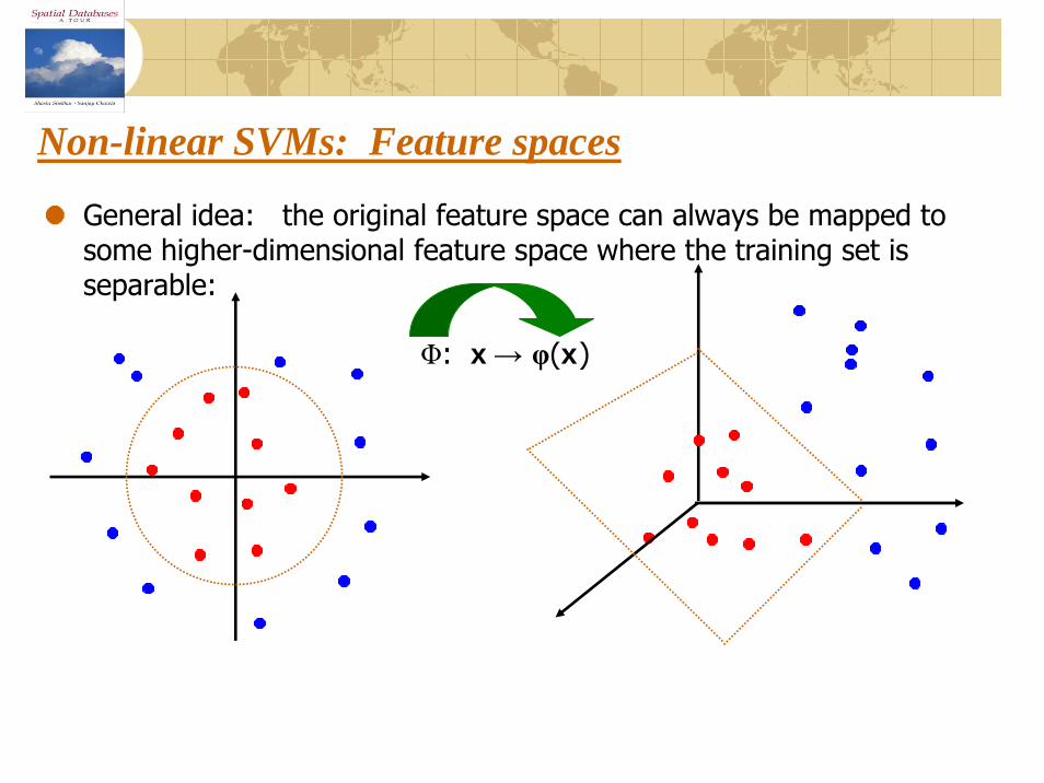
Non-linear SVMs: Feature spaces

General idea: the original feature space can always be mapped to some higher-dimensional feature space where the training set is separable:

Φ: x→ φ(x)

SVM applicationsSVMs were originally proposed by Boser, Guyon and Vapnik in 1992 and gained increasing popularity in late 1990s.SVMs are currently among the best performers for a number of classification tasks ranging from text to genomic data.SVMs can be applied to complex data types beyond feature vectors (e.g. graphs, sequences, relational data) by designing kernel functions for such data.SVM techniques have been extended to a number of tasks such as regression [Vapnik et al. ’97], principal component analysis [Schölkopf et al. ’99], etc. Most popular optimization algorithms for SVMs use decomposition to hill-climb over a subset of αi’s at a time, e.g. SMO [Platt ’99] and [Joachims ’99]Tuning SVMs remains a black art: selecting a specific kernel and

parameters is usually done in a try-and-see manner.

33

Instance-Based Learning

Unlike other learning algorithms, does not involve construction of an explicit abstract generalization but classifies new instances based on direct comparison and similarity to known training instances.Training can be very easy, just memorizing training instances.Testing can be very expensive, requiring detailed comparison to all past training instances.Also known as:

Case-based Exemplar-basedNearest NeighborMemory-basedLazy Learning

34

Similarity/Distance MetricsInstance-based methods assume a function for determining the similarity or distance between any two instances.For continuous feature vectors, Euclidian distance is the generic choice:

∑=

−=n

pjpipji xaxaxxd

1

2))()((),(

Where ap(x) is the value of the pth feature of instance x.• For discrete features, assume distance between two

values is 0 if they are the same and 1 if they are different (e.g. Hamming distance for bit vectors).

• To compensate for difference in units across features, scale all continuous values to the interval [0,1].

35

Other Distance Metrics

Mahalanobis distanceScale-invariant metric that normalizes for variance.

Cosine SimilarityCosine of the angle between the two vectors.Used in text and other high-dimensional data.

Pearson correlationStandard statistical correlation coefficient.Used for bioinformatics data.

Edit distanceUsed to measure distance between unbounded length strings.Used in text and bioinformatics.

36

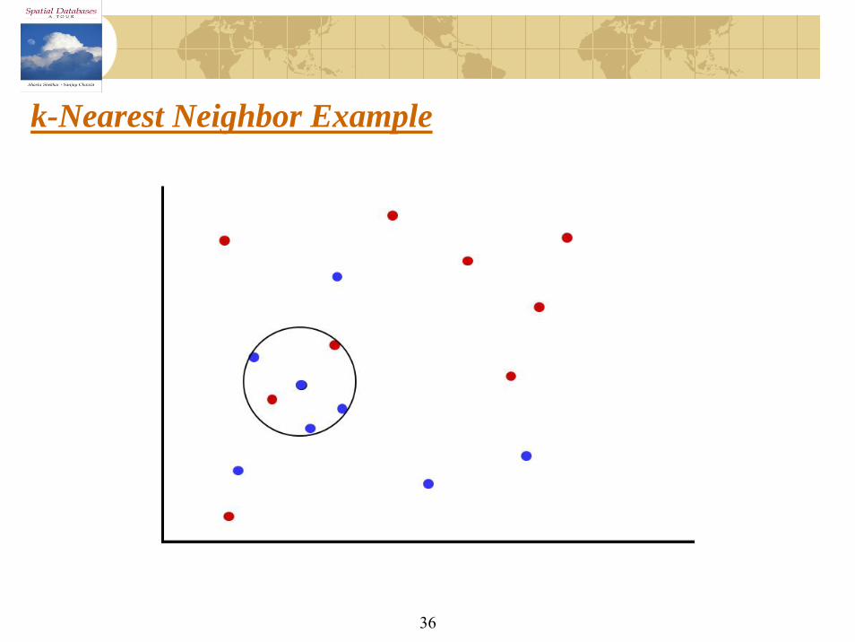
k-Nearest Neighbor Example

37

Implicit Classification FunctionAlthough it is not necessary to explicitly calculate it, the learned classification rule is based on regions of the feature space closest to each training example.For 1-nearest neighbor with Euclidian distance, the Voronoi diagram gives the complex polyhedra segmenting the space into the regions closest to each point.

38

Efficient Indexing

Linear search to find the nearest neighbors is not efficient for large training sets.Indexing structures can be built to speed testing.For Euclidian distance, a kd-tree can be built that reduces the expected time to find the nearest neighbor to O(log n) in the number of training examples.

Nodes branch on threshold tests on individual features and leaves terminate at nearest neighbors.

Other indexing structures possible for other metrics or string data.

Inverted index for text retrieval.

39

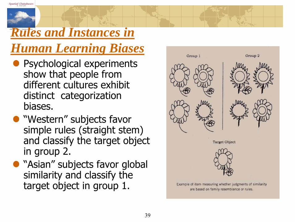
Rules and Instances inHuman Learning Biases

Psychological experiments show that people from different cultures exhibit distinct categorization biases.“Western” subjects favor simple rules (straight stem) and classify the target object in group 2.“Asian” subjects favor global similarity and classify the target object in group 1.

40

Other Issues

Can reduce storage of training instances to a small set of representative examples.

Support vectors in an SVM are somewhat analogous.Can be used for more complex relational or graph data.

Similarity computation is complex since it involves some sort ofgraph isomorphism.

Can be used in problems other than classification.Case-based planningCase-based reasoning in law and business.

41

Bayesian Networks

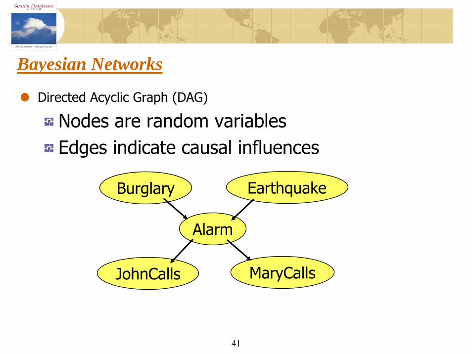
Directed Acyclic Graph (DAG)

Nodes are random variablesEdges indicate causal influences

Burglary Earthquake

Alarm

JohnCalls MaryCalls

42

Conditional Probability TablesEach node has a conditional probability table (CPT) that gives the probability of each of its values given every possible combination of values for its parents (conditioning case).

Roots (sources) of the DAG that have no parents are given prior probabilities.

Burglary Earthquake

Alarm

JohnCalls MaryCalls

P(B)

.001

P(E)

.002

B E P(A)T T .95T F .94F T .29F F .001

A P(M)T .70F .01

A P(J)T .90F .05

43

Bayes Net Inference

Given known values for some evidence variables, determine the posterior probability of some query variables.Example: Given that John calls, what is the probability that there is a Burglary?

Burglary Earthquake

Alarm

JohnCalls MaryCalls

???John calls 90% of the time thereis an Alarm and the Alarm detects94% of Burglaries so peoplegenerally think it should be fairly high.

However, this ignores the priorprobability of John calling.

44

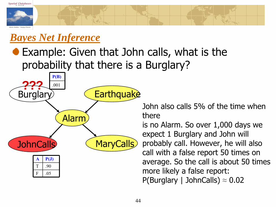
Bayes Net InferenceExample: Given that John calls, what is the probability that there is a Burglary?

Burglary Earthquake

Alarm

JohnCalls MaryCalls

???P(B)

.001

John also calls 5% of the time when thereis no Alarm. So over 1,000 days we expect 1 Burglary and John will probably call. However, he will also call with a false report 50 times on average. So the call is about 50 times more likely a false report:P(Burglary | JohnCalls) ≈ 0.02

A P(J)T .90F .05

Learning EnsemblesLearn multiple alternative definitions of a concept using different training data or different learning algorithms.Combine decisions of multiple definitions, e.g. using weighted voting.

46

Value of Ensembles

When combing multiple independent anddiverse decisions each of which is at least more accurate than random guessing, random errors cancel each other out, correct decisions are reinforced.Human ensembles are demonstrably better

How many jelly beans in the jar?: Individual estimates vs. group average.Who Wants to be a Millionaire: Expert friend vs. audience vote.

47

Experimental Results on Ensembles(Freund & Schapire, 1996; Quinlan, 1996)

Ensembles have been used to improve generalization accuracy on a wide variety of problems.On average, Boosting provides a larger increase in accuracy than Bagging.Boosting on rare occasions can degrade accuracy.Bagging more consistently provides a modest improvement.Boosting is particularly subject to over-fitting when there is significant noise in the training data.

48

K-Fold Cross Validation Comments

Every example gets used as a test example once and as a training example k–1 times.All test sets are independent; however, training sets overlap significantly.Measures accuracy of hypothesis generated for [(k–1)/k]⋅|D| training examples.Standard method is 10-fold.If k is low, not sufficient number of train/test trials; if k is high, test set is small and test variance is high and run time is increased.If k=|D|, method is called leave-one-out cross validation.