introduction to statistical inference - north carolina state university
TRANSCRIPT

Introduction to Statistical Inference
Introduction to Statistical Inference
Jayanta Kumar Pal
SAMSISAMSI/CRSC Undergraduate Workshop at NCSU
May 22, 2007

Introduction to Statistical Inference
Outline
1 Introduction
2 Some important conceptsEstimationHypothesis testing
3 Example 1 : binomial data
4 Example 2 : normal data

Introduction to Statistical Inference
Introduction
Outline
1 Introduction
2 Some important conceptsEstimationHypothesis testing
3 Example 1 : binomial data
4 Example 2 : normal data

Introduction to Statistical Inference
Introduction
Statistical Inference
There are three steps for Statistical methods.Data collection.Data presentationData analysis.
We focus on the third and final step - the inference.
Seek to draw conclusions based on the data.
Important aspect - the underlying model.

Introduction to Statistical Inference
Introduction
Parametric model
Prior belief or notion dictates the choice of model.
Sometimes, a glance at the plot shows why some specific modelmay be of interest.

Introduction to Statistical Inference
Introduction
Parametric model
Prior belief or notion dictates the choice of model.
Sometimes, a glance at the plot shows why some specific modelmay be of interest.

Introduction to Statistical Inference
Introduction
What is the possible underlying model?
0 0.5 1 1.5 2 2.5 3 3.5 4 4.5 52
4
6
8
10
12
14
A linear fit !!!

Introduction to Statistical Inference
Introduction
What is the possible underlying model?
0 0.5 1 1.5 2 2.5 3 3.5 4 4.5 52
4
6
8
10
12
14
A linear fit !!!

Introduction to Statistical Inference
Introduction
A quadratic fit might be the winner?
0 0.5 1 1.5 2 2.5 3 3.5 4 4.5 5−30
−20
−10
0
10
20
30
40

Introduction to Statistical Inference
Some important concepts
Outline
1 Introduction
2 Some important conceptsEstimationHypothesis testing
3 Example 1 : binomial data
4 Example 2 : normal data

Introduction to Statistical Inference
Some important concepts
Quantities of interest
Parameter : some unknown but fixed quantity. Does not dependon data.
Statistic : A quantity that depends on data. Computed from thesample.
Estimator : A statistic to predict/substitute the parameter.

Introduction to Statistical Inference
Some important concepts
Quantities of interest
Parameter : some unknown but fixed quantity. Does not dependon data.
Statistic : A quantity that depends on data. Computed from thesample.
Estimator : A statistic to predict/substitute the parameter.

Introduction to Statistical Inference
Some important concepts
Quantities of interest
Parameter : some unknown but fixed quantity. Does not dependon data.
Statistic : A quantity that depends on data. Computed from thesample.
Estimator : A statistic to predict/substitute the parameter.

Introduction to Statistical Inference
Some important concepts
Statistical methods
There are two main problems of statistical analysis.EstimationTesting of hypothesis.
We will briefly discuss them here. Our examples will illustratethe difference between them.

Introduction to Statistical Inference
Some important concepts
Statistical methods
There are two main problems of statistical analysis.EstimationTesting of hypothesis.
We will briefly discuss them here. Our examples will illustratethe difference between them.

Introduction to Statistical Inference
Some important concepts
Statistical methods
There are two main problems of statistical analysis.EstimationTesting of hypothesis.
We will briefly discuss them here. Our examples will illustratethe difference between them.

Introduction to Statistical Inference
Some important concepts
Estimation
Estimation
Estimation can be of two types.
Point estimation : We seek to specify a predictive value for theparameter.
Interval estimation : The goal is to specify a range of candidatevalues for the parameter.
We try to discuss them briefly using examples.

Introduction to Statistical Inference
Some important concepts
Estimation
Point estimation
Consider the following example :The North Carolina State University seeks to figure out thefraction of monthly expenses spent by its students on differentcategories.
Question : What is the percentage spent on groceries andmerchandize?
Data : We collect data on 1000 random students across thecampus and record their expenditure pattern.

Introduction to Statistical Inference
Some important concepts
Estimation
Point estimation
We observe that the average spent on the purchases is 21%.
Parameter : the unknown fraction spent on them.Statistic : average of the proportions in the 1000 students.
This average is an estimator of the unknown parameter.
This is known as point estimation.
However, this does not tell us about how close we are to theactual fraction, or how accurate our estimator is.
Introduction to Statistical Inference
Some important concepts
Estimation
Interval estimation
Instead of specifying the value at a point, one looks for a rangeof values as plausible, e.g. 19% to 23%.
The goal is to ascertain some probability for such an interval, orideally find an interval with a pre-specified probability (like .95or .99) attached to it.

Introduction to Statistical Inference
Some important concepts
Hypothesis testing
Hypothesis testing
Our next example comes from the D.M.V.The D.M.V. wants to apprise the effect of air-bags in reducingthe risk of death in road accidents.
Question : Does having air-bag reduce the chance of death incollisions?
Hypothesis 1 : The chances remain same. This is known as thenull hypothesis (status quo)Hypothesis 2 : The risk is less for cars having air-bags. This isthe alternate hypothesis.

Introduction to Statistical Inference
Some important concepts
Hypothesis testing
Hypothesis testing
The data from last year shows about 11% among the air-bag caroccupants succumb to fatal injuries.
In the cars without the safety equipments, the correspondingfigure is 14%.
Question : Is the rise in percentage significant to conclude infavor of Hypothesis 2? Or is this just a chance variation, and canHypothesis 1 not be overwhelmingly ruled out?
Introduction to Statistical Inference
Some important concepts
Hypothesis testing
We will discuss the estimation procedure with a few more examples.

Introduction to Statistical Inference
Example 1 : binomial data
Outline
1 Introduction
2 Some important conceptsEstimationHypothesis testing
3 Example 1 : binomial data
4 Example 2 : normal data

Introduction to Statistical Inference
Example 1 : binomial data
Part-time jobs in campus
A study is conducted among the Duke University students. 5undergraduates are chosen at random and asked whether theyreceive their spending money from part-time jobs.
Name Age Year Part-timerLesley Pickering 19 Junior NO
Jason Gullian 18 Freshman YESErin McClintic 20 Junior NO
Stacey Culp 19 Sophomore NOFred Almirall 21 Senior YES

Introduction to Statistical Inference
Example 1 : binomial data
Estimation
An unknown fraction π of the pool of students have part-timejobs.
We want to estimate that unknown π.
Given any value of π ∈ [0, 1], what are the chances of having arandom sample of 5 students with 2 of them doing such jobs?
Also, what is the most likely value of π that can generate such asample?
Normal guess : π = 25 = .4.

Introduction to Statistical Inference
Example 1 : binomial data
What is more likely?
This comes from a binomial distribution, which is discrete innature.
If we know the value of π, we can write the probability of thesequences.
If π = .2, the probability of such an occurrence is.8× .2× .8× .8× .2 = .02048.
If π = .5, the probability becomes.5× .5× .5× .5× .5 = .03125.
Conclusion : π = .5 is more likely to π = .2.

Introduction to Statistical Inference
Example 1 : binomial data
Maximum likelihood estimator
Of all possible values of π ∈ [0, 1], which one has the largestpossibility of producing the data?
In particular, which value of π has the largest likelihood?
It will be called the maximum likelihood estimator.

Introduction to Statistical Inference
Example 1 : binomial data
MLE computation
For some specific value of π, the probability of the data is givenby
L(π) = (1− π)π(1− π)(1− π)π= π2 − 3π3 + 3π4 − π5
⇒ ddπ
L(π) = 2π − 9π2 + 12π3 − 5π4
= π(1− π)2(2− 5π)

Introduction to Statistical Inference
Example 1 : binomial data
MLE computation
Therefore, ddπL(π) = 0 if π = 0, 1 or 2
5 .
Now, L(0) = 0 = L(1).Further,
d2
dπ2 L(π) = 2− 18π+ 36π2− 20π3 = 2(1− π)(1− 8π+ 10π2)
which is negative if π = .4.
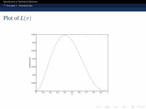
Therefore, π = .4 is the MLE. We denote it by π̂.

Introduction to Statistical Inference
Example 1 : binomial data
MLE computation
Therefore, ddπL(π) = 0 if π = 0, 1 or 2
5 .
Now, L(0) = 0 = L(1).Further,
d2
dπ2 L(π) = 2− 18π+ 36π2− 20π3 = 2(1− π)(1− 8π+ 10π2)
which is negative if π = .4.
Therefore, π = .4 is the MLE. We denote it by π̂.

Introduction to Statistical Inference
Example 1 : binomial data
MLE computation
Therefore, ddπL(π) = 0 if π = 0, 1 or 2
5 .
Now, L(0) = 0 = L(1).Further,
d2
dπ2 L(π) = 2− 18π+ 36π2− 20π3 = 2(1− π)(1− 8π+ 10π2)
which is negative if π = .4.
Therefore, π = .4 is the MLE. We denote it by π̂.
Introduction to Statistical Inference
Example 1 : binomial data
How likely are other plausible values of π
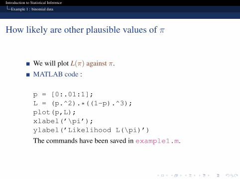
We will plot L(π) against π.
MATLAB code :
p = [0:.01:1];L = (p.^2).*((1-p).^3);plot(p,L);xlabel(’\pi’);ylabel(’Likelihood L(\pi)’)
The commands have been saved in example1.m.
Introduction to Statistical Inference
Example 1 : binomial data
Plot of L(π)
0 0.1 0.2 0.3 0.4 0.5 0.6 0.7 0.8 0.9 10
0.005
0.01
0.015
0.02
0.025
0.03
0.035
π
Like
lihoo
d L(
π)

Introduction to Statistical Inference
Example 1 : binomial data
Exercise 1
You have a bag of marbles, millions in number.
A fraction π of them are white, rest are red.
You draw 10 at random, and the colors turn out to beW.R.W.W.W.R.R.W.R.W.
Compute the MLE for π and use MATLAB to see how likely arethe other values between [0, 1].

Introduction to Statistical Inference
Example 2 : normal data
Outline
1 Introduction
2 Some important conceptsEstimationHypothesis testing
3 Example 1 : binomial data
4 Example 2 : normal data

Introduction to Statistical Inference
Example 2 : normal data
Guyana rainfall data
We have data that can be modeled as coming from a Normaldistribution with mean µ and standard deviation σ (bothunknown).
In Guyana, South America, we record the annual rainfall in thelast 6 years.
Year rainfall2001 95"2002 118"2003 85"2004 154"2005 102"2006 96"
Introduction to Statistical Inference
Example 2 : normal data
Normal likelihood
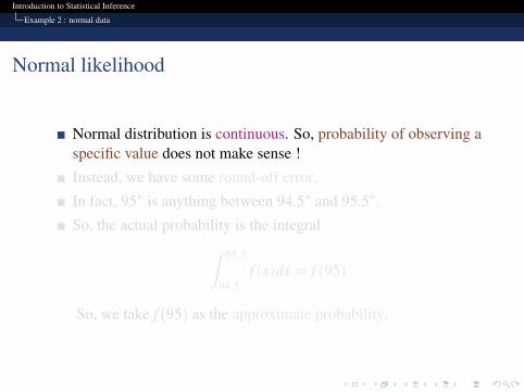
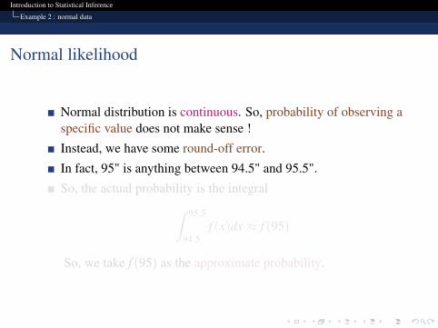
Normal distribution is continuous. So, probability of observing aspecific value does not make sense !
Instead, we have some round-off error.
In fact, 95" is anything between 94.5" and 95.5".
So, the actual probability is the integral∫ 95.5
94.5f (x)dx ≈ f (95)
So, we take f (95) as the approximate probability.
Introduction to Statistical Inference
Example 2 : normal data
Normal likelihood
Normal distribution is continuous. So, probability of observing aspecific value does not make sense !
Instead, we have some round-off error.
In fact, 95" is anything between 94.5" and 95.5".
So, the actual probability is the integral∫ 95.5
94.5f (x)dx ≈ f (95)
So, we take f (95) as the approximate probability.

Introduction to Statistical Inference
Example 2 : normal data
Normal likelihood
Also, the rainfall amounts in different years are considered asindependent.
Caution : this is slightly dubious. Ideally we should treat them astime-series but that is beyond our discussion here.
So, the likelihood of the data is f (95).f (118) . . . f (96).For a specific µ and σ, the likelihood is
L(µ, σ) = f (95, µ, σ).f (118, µ, σ) . . . f (96, µ, σ)

Introduction to Statistical Inference
Example 2 : normal data
Plot using MATLAB
We can plot that function using MATLAB.
For any µ, σ and vector X, the functionnormpdf(X,mu,sigma) returns a vector of f-values.
Likelihood is a product of those values.
clear allX = [95,118, 85,154,102,96]’;mu = 100;sigma = 10;L(mu,sigma) = prod(normpdf(X,mu,sigma))

Introduction to Statistical Inference
Example 2 : normal data
Possible values of µ and σ
The data are between 85 and 154.
So, µ, as a measure of central tendency, should be between thisvalues.
Range of the data is 154-85=69.
σ is likely to be between 0 and 70.
We plot L(µ, σ) for those values.

Introduction to Statistical Inference
Example 2 : normal data
Possible values of µ and σ
The data are between 85 and 154.
So, µ, as a measure of central tendency, should be between thisvalues.
Range of the data is 154-85=69.
σ is likely to be between 0 and 70.
We plot L(µ, σ) for those values.

Introduction to Statistical Inference
Example 2 : normal data
Possible values of µ and σ
The data are between 85 and 154.
So, µ, as a measure of central tendency, should be between thisvalues.
Range of the data is 154-85=69.
σ is likely to be between 0 and 70.
We plot L(µ, σ) for those values.

Introduction to Statistical Inference
Example 2 : normal data
Plot of the function L(µ, σ)
MATLAB code :
mu = [85:.3:154];sigma = [0:.5:70];L = zeros(length(mu),length(sigma));for i = 1:length(mu)
for j = 1:length(sigma)L(i,j) = prod(normpdf(X,mu(i),sigma(j)));
endend
surf(mu,sigma, L’)xlabel(’\sigma’)ylabel(’\mu’)

Introduction to Statistical Inference
Example 2 : normal data
Plot of L(µ, σ)

Introduction to Statistical Inference
Example 2 : normal data
Computation of the MLE-s
L(µ, σ) = f (95, µ, σ).f (118, µ, σ) . . . f (96, µ, σ)
Recall that
f (x, µ, σ) =1√2πσ
exp−(x− µ)2
2σ2
Therefore
L(µ, σ) =1
8π3σ6 exp(− 12σ2 {(95− µ)2 + . . .+ (96− µ)2})
=1
8π3σ6 exp(− 12σ2 {6µ
2 − 1300µ+ 73510})

Introduction to Statistical Inference
Example 2 : normal data
Computation of the MLE-sTaking logarithm
l(µ, σ) = C − 6 logσ − 1σ2 {3µ
2 − 650µ+ 36755}
Taking partial derivatives,
∂l∂µ
= − 1σ2 {6µ− 650}
and∂l∂σ
= − 6σ
+2σ3 {3µ
2 − 650µ+ 36755}
Setting ∂l∂µ = ∂l
∂σ = 0, we get
µ = 108.33, σ = 22.7061

Introduction to Statistical Inference
Example 2 : normal data
Computation of the MLE-sTaking logarithm
l(µ, σ) = C − 6 logσ − 1σ2 {3µ
2 − 650µ+ 36755}
Taking partial derivatives,
∂l∂µ
= − 1σ2 {6µ− 650}
and∂l∂σ
= − 6σ
+2σ3 {3µ
2 − 650µ+ 36755}
Setting ∂l∂µ = ∂l
∂σ = 0, we get
µ = 108.33, σ = 22.7061

Introduction to Statistical Inference
Example 2 : normal data
Computation of the MLE-sTaking logarithm
l(µ, σ) = C − 6 logσ − 1σ2 {3µ
2 − 650µ+ 36755}
Taking partial derivatives,
∂l∂µ
= − 1σ2 {6µ− 650}
and∂l∂σ
= − 6σ
+2σ3 {3µ
2 − 650µ+ 36755}
Setting ∂l∂µ = ∂l
∂σ = 0, we get
µ = 108.33, σ = 22.7061

Introduction to Statistical Inference
Example 2 : normal data
Exercise 2
Enter the data on heights (as collected by Dhruv).
Assume that the data comes from a normal distribution.
Plot the likelihood as a function of µ and σ. (Use the range of thedata for the range of µ and σ.
Find the mean and the standard deviation of the data. (inMATLAB use the functions mean(x) and std(x,1))
Check (visually), that the mean and SD corresponds for the MLEfor µ and σ respectively.

Introduction to Statistical Inference
Example 2 : normal data
Conclusion
As shown in the examples, the MLE of (multiple) parameters canbe done simultaneously.
In both examples, there is an utility function that we need tomaximize.
Similarly, there may be a cost function attached to theparameters that we can minimize to get estimators.
The least squares estimation or the least absolute deviationmethods are from that class of estimation.
Enjoy your stay here in Raleigh !!!