introduction to statistical learning theory -
TRANSCRIPT

Introduction to Statistical LearningTheory
Petra Philips
1 Friedrich Miescher Laboratory, TübingenVorlesung WS 2007/2008
Eberhard-Karls-Universität Tübingen
27 November 2007
http://www.fml.mpg.de/raetsch/lectures/amsa07

Retrospection
G. Rätsch, C.S. Ong and P. Philips: Advanced Methods for Sequence Analysis, Page 2

Supervised Learning in a Nutshell
G. Rätsch, C.S. Ong and P. Philips: Advanced Methods for Sequence Analysis, Page 3
GivenTraining data : A finite set of examples xi ∈ X and theirassociated labels yi ∈ Y.
WantedThe ’best’ estimator modelling the relationship betweenthe xi and the associated labels yi, i.e. the ’best’ function
h : X → Y.
Approach
Restrict possible functions (e.g. hyperplanes).Quantify ’best’ as the optimum of some computableobjective function (usually error on training data).Evaluate prediction performance on new test data .

Challenge
G. Rätsch, C.S. Ong and P. Philips: Advanced Methods for Sequence Analysis, Page 4
Is there an a priori way to guarantee good performance?

Probabilistic Learning Model
G. Rätsch, C.S. Ong and P. Philips: Advanced Methods for Sequence Analysis, Page 5
AssumptionAll data is generated by the same hidden probabilisticsource!
Formallyp is an unknown joint probability distribution over X×Y
Training data ((x1, y1), . . . , (xn, yn)) is iid ∼ p
Loss: the error for a particular example `(h(xi), yi).Aim: find best h∗∗ that minimizes risk
L(h) = EX×Y l(Y, h(X)) =
∫`(h(x), y)dp.

Probabilistic Learning Model
G. Rätsch, C.S. Ong and P. Philips: Advanced Methods for Sequence Analysis, Page 6
AssumptionAll data is generated by the same hidden probabilisticsource!
Formallyp is an unknown joint probability distribution over X×Y
Training data ((x1, y1), . . . , (xn, yn)) is iid ∼ p
Loss: the error for a particular example `(h(xi), yi).Aim: find best h∗ ∈ H that minimizes risk
L(h) = EX×Y l(Y, h(X)) =
∫`(h(x), y)dp.

Probabilistic Learning Model
G. Rätsch, C.S. Ong and P. Philips: Advanced Methods for Sequence Analysis, Page 7
AssumptionAll data is generated by the same hidden probabilisticsource!
Formallyp is an unknown joint probability distribution over X×Y
Training data ((x1, y1), . . . , (xn, yn)) is iid ∼ p
Loss: the error for a particular example `(h(xi), yi).Aim: find best h∗ ∈ H that minimizes risk
L(h) = EX×Y l(Y, h(X)) =
∫`(h(x), y)dp.
ERM: find best hn ∈ H that minimizes empirical risk
Lemp(h) =1
n
n∑i=1
`(h(xi), yi).
Questions
G. Rätsch, C.S. Ong and P. Philips: Advanced Methods for Sequence Analysis, Page 8
How can we know we are doing ’the right thing’?How to restrict the possible set of functions?Occam’s Razor Of two equivalent models choose the
simplest one. ?Can we quantify the ’complexity’ of a learning problem?Is more data always better data?How much data do we need?

Statistical Learning Theory
G. Rätsch, C.S. Ong and P. Philips: Advanced Methods for Sequence Analysis, Page 9
Provides a theoretical framework to study thesequestions.Started with ? which led to VC-Theory and SVM.Models the machine learning setting as astatistical phenomenon .
Answers are probabilistic in nature.Tools: statistics, functional analysis, empiricalprocesses, combinatorics, high-dimensional ge-ometry, complexity theory.Newer view: ??.

Challenge Question
G. Rätsch, C.S. Ong and P. Philips: Advanced Methods for Sequence Analysis, Page 10
Is L(hn) small, i.e. L(hn) ≈ L(h∗∗)?
Magics?

Approximation & Estimation Error
G. Rätsch, C.S. Ong and P. Philips: Advanced Methods for Sequence Analysis, Page 11
L(hn)− L(h∗∗) = L(hn)− L(h∗) + L(h∗)− L(h∗∗)
H large
small approximation erroroverfitting
H small
large approximation errorbetter generalization but poor performance
Model selectionChoose H to get an optimal tradeoff between approxi-mation and estimation error.

Estimation Error
G. Rätsch, C.S. Ong and P. Philips: Advanced Methods for Sequence Analysis, Page 12
L(h∗)− L(hn) ?
depends on training datadepends on H
depends on how algorithm chooses hn
depends on unknown p through h∗ and risk
For ERM use uniform differences trick!
Uniform differences
|L(h∗)− L(hn)| ≤ 2 suph∈H
|Lemp(h)− L(h)|

Empirical and Actual Risk
G. Rätsch, C.S. Ong and P. Philips: Advanced Methods for Sequence Analysis, Page 13
Lemp(h) ≈ L(h) ?
Asymptotics: Law of Large NumbersFor any fixed h, |Lemp(h)− L(h)| −→ 0 as n −→∞.
Finite Sample Result [Chernoff-Hoeffding]For any fixed h, with high probability
|Lemp(h)− L(h)| ≈ 1√n.
Does this mean that ERM finds optimal estimator h∗ whentraining sample is getting large?
Empirical and Actual Risk
G. Rätsch, C.S. Ong and P. Philips: Advanced Methods for Sequence Analysis, Page 14
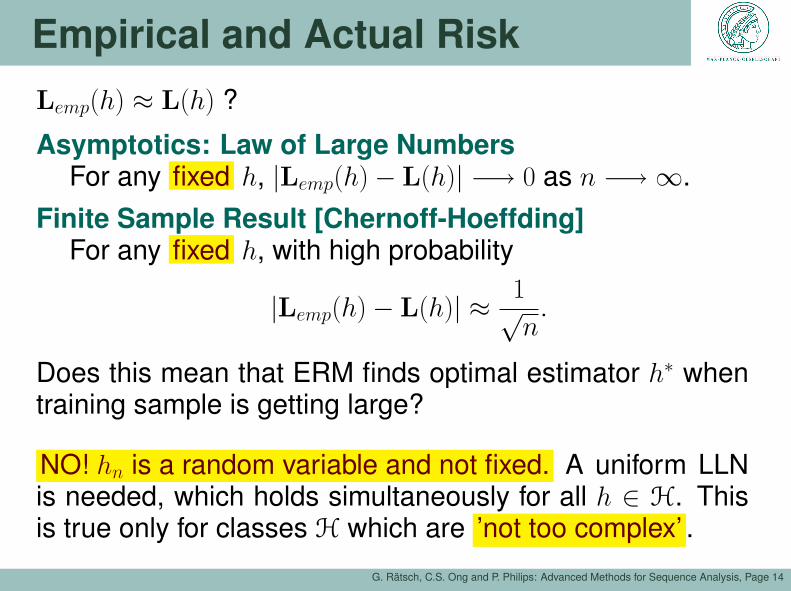
Lemp(h) ≈ L(h) ?
Asymptotics: Law of Large NumbersFor any fixed h, |Lemp(h)− L(h)| −→ 0 as n −→∞.
Finite Sample Result [Chernoff-Hoeffding]For any fixed h, with high probability
|Lemp(h)− L(h)| ≈ 1√n.
Does this mean that ERM finds optimal estimator h∗ whentraining sample is getting large?
NO! hn is a random variable and not fixed. A uniform LLNis needed, which holds simultaneously for all h ∈ H. Thisis true only for classes H which are ’not too complex’ .

Estimation Error
G. Rätsch, C.S. Ong and P. Philips: Advanced Methods for Sequence Analysis, Page 15
L(hn)− L(h∗) ?
Uniform differences
|L(hn)− L(h∗)| ≤ 2 suph∈H
|Lemp(h)− L(h)|
Finite Sample Results
One fixed function: |Lemp(h)− L(h)| ≈ 1/√
n
H finite: suph∈H |Lemp(h)− L(h)| ≈√
log(|H|)/√
n
H infinite: ?
VC Dimension
G. Rätsch, C.S. Ong and P. Philips: Advanced Methods for Sequence Analysis, Page 16
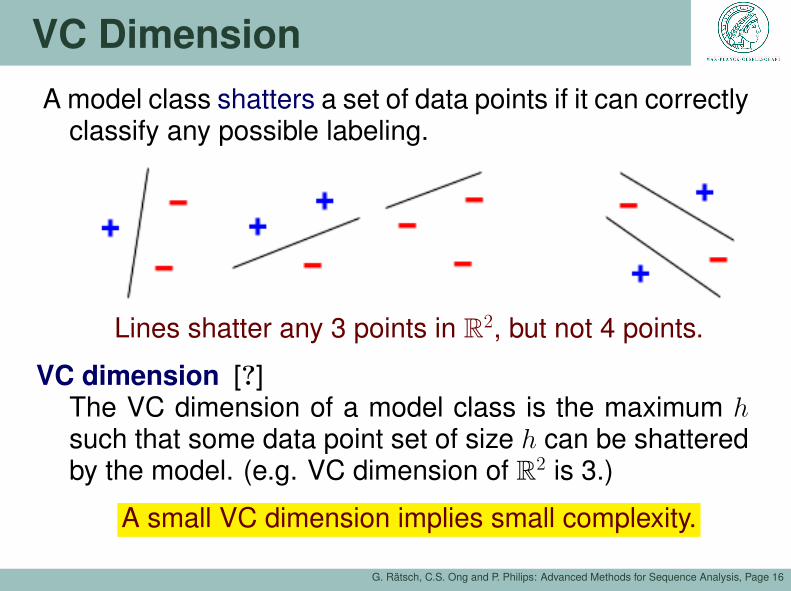
A model class shatters a set of data points if it can correctlyclassify any possible labeling.
Lines shatter any 3 points in R2, but not 4 points.
VC dimension [?]The VC dimension of a model class is the maximum hsuch that some data point set of size h can be shatteredby the model. (e.g. VC dimension of R2 is 3.)
A small VC dimension implies small complexity.

Why?
G. Rätsch, C.S. Ong and P. Philips: Advanced Methods for Sequence Analysis, Page 17
Shattering Coefficient: The number of distinct patterns afunction class H can produce on a sample x.
Sn(H,x) = |H/x|
Sauer-Shelah Lemma:
Sn(H,x) ≤VC(H)∑
i=1
(n
i
)∼ nVC(H)
A function class ’behaves’ on sample like a class withcardinality nVC(H).

Optimal and Empirical Estimator
G. Rätsch, C.S. Ong and P. Philips: Advanced Methods for Sequence Analysis, Page 18
L(h∗) ≈ L(hn) ?
Uniform differences
|L(h∗)− L(hn)| ≤ 2 suph∈H
|Lemp(h)− L(h)|
Finite Sample Results
One fixed function: |Lemp(h)− L(h)| ≈ 1/√
n
H finite: suph∈H |Lemp(h)− L(h)| ≈√
log(|H|)/√
n
H infinite:suph∈H |Lemp(h)− L(h)| ≈√
VC(H)log(n)/√
n
All results hold with high probability overthe random draw of training samples!

Beyond VC Dimension
G. Rätsch, C.S. Ong and P. Philips: Advanced Methods for Sequence Analysis, Page 19
Rethinking: A function class ’behaves’ in the worst caseon sample like a class with cardinality VC(H).
Rademacher Averages: Average of highest correlation offunctions with n random patterns εi = +/− 1.
Rn(H) = EX,ε
(suph∈H
∣∣∣∣∣n∑
i=1
εih(Xi)
∣∣∣∣∣)
Extends theory to general loss functions.Finite VC dimension leads to upper estimate.More sophisticated mathematical machinery whichavoids union bound.Better understanding of learning phenomenon.
??

Implications
G. Rätsch, C.S. Ong and P. Philips: Advanced Methods for Sequence Analysis, Page 20
VC dimensions are meaningful complexity measures.Do model selection by minimizing VC dimension.More data gives more likely a good predictor.

Larger Margin Classifiers
G. Rätsch, C.S. Ong and P. Philips: Advanced Methods for Sequence Analysis, Page 21
Large Margin ⇒ Small VC dimensionHyperplane classifiers with large margin have small VCdimension [?].
Maximum Margin ⇒ Minimum ComplexityMinimize complexity by maximizing margin (irrespectiveof the dimension of the space).

Model Selection In Practice
G. Rätsch, C.S. Ong and P. Philips: Advanced Methods for Sequence Analysis, Page 22
VC-type complexities are hard to compute, but
Lemp(h) ∼ L(h) ⇒ Lemp2(h) ∼ L(h)
Strategy: Choose among good empirical hypotheses theones which are similar on independent samples.
Training Sample
Sample 2Sample 1

Validation
G. Rätsch, C.S. Ong and P. Philips: Advanced Methods for Sequence Analysis, Page 23
Model selection and error estimation.Randomly chosen subsets of disjoint training, validation,test data.Works well for large data sets.
Training Validation Test

Crossvalidation
G. Rätsch, C.S. Ong and P. Philips: Advanced Methods for Sequence Analysis, Page 24
K-fold Crossvalidation:Splitting into K sample sets.K times training on K-1-sets.Error estimation through averaging on each of the K’left-out’ test sets.K trades bias vs. variance (in practice K=5,10).

Summary - SLT
G. Rätsch, C.S. Ong and P. Philips: Advanced Methods for Sequence Analysis, Page 25
Provides a statistical framework to study learning algorithms.
Quantifies the generalization ability in terms of
complexity of estimator functions
number of training examples.
Results are probabilistic in nature (confidences).
Results teach us
When and why our intuitive solutions were right (SVM, boosting,some forms of crossvalidation).
Why and how to restrict class of estimators and to regularize.
That more data is best because it increases confidence in result.
But: Limited model, many questions not yet understood!