1

Introduction to Statistics and Biostatistics:

Statistics is used by all of us in our day to day life, may not be in the most complex form but

in general simple logic we provide for daily occurrences based on simple analytical

probability. The examples for statistics range from the outcomes of coin tossing experiments

to public opinion polls, predicting the general public consensus regarding state elections.

Statistics finds its use in fields as varied as sociology to economics to health sciences to

mathematics. From the Lattice LotkaVolterra model for studying population model (1) to

using Fourier statistics to portray human faces (2). Such varied use of statistics has also

contributed to personalised advancement of specialised fields in statistics.

The various fields of statistics widely used include astrostatistics, biostatistics, business

analytics, environmental statistics, population ecology, quantitative psychology, statistical

finance, statistical mechanic, statistical physics, statistical thermodynamics, etc.

In this chapter, we shall start from looking into the population types, sampling techniques and

basic analysis. We will discuss different types of data, frequency distribution, frequency

tables. A data representation is an important use of statistics and enables us to achieve finer

interpretation of the given data. In the section, we will look at various representation methods

along with the measures of central tendency. Simultaneously we shall discuss discrete and

continuous distributions and concept of confidence intervals, which will take us deeper into

the understanding of a range of predictability in statistics. This study will enable us to

proceed with hypothesis testing. In this chapter,we shall look further in basic analysis of

variance, correlation, regression. It will include the basic idea of biostatistics.

Definitions:

Datacan be defined as any information, collected in raw or organised form based on

observations (includes visual interpretations, measured quantities, survey responses, etc.),

which suitably refer to a set of defined conditions, ideas or objects.

Statistics is the study of the planning experiments followed by collecting, organizing,

analysing, interpreting and presenting data. So it deals with the overall establishment of

experiments/ cases, beginning from design of experiment to inferring and presenting the

resulting data obtained. Statistics can be broadly categorized into two types: descriptive and

inferential statistics.

Population refers to the complete collection of all elements (scores, people, measurements,

2

and so on) from where the data has been obtained. The collection includes all subjects to be

studied.

Census refers to the systematic collection of data from every member of the population and

is usually recorded periodically at regular intervals.

Sample refers to a sub-collection of elements selected from a population, and the data is

collected and assumed to be representing the whole population.

Descriptive statistics is used to describe the population under study using statistical

procedures, and the results cannot be extended to a larger population. The results obtained

facilitate better organization of data and information about the population and is limited to the

same. Therefore, descriptive statistics is useful when the result are used for the population

under study, and need not be extended further. Examples of descriptive statistics include

frequency distributions, measures of central tendency and graphical representations.

Inferential statistics as the name suggests is involved in drawing inferences about a larger

population, based on a study conducted on a sample. In this case it is important to

selectcarefully the sample for a study as the results obtained thereby, will be extended and

shall be applicable to the whole concerned population. Several tests of significance such as

Chi-square or t-test allow us to decide whether the results of our analysis on the samples are

significantly representing the population it is supposed to represent or not. Correlation

analyses, regression analyses, ANOVA are examples of inferential statistics.

Discrete variables either have a finite number of values or a counted number of possible

values. In other words, they can have only certain values and none in between. For example,

the number of students on a class on roll can be 44 or 45, but can never be in between these

two.

Continuous variables can have many possible values; they may take any value in a given

range without gaps or intervals. However, they may have intermediate discrete values

depending on the measurement strategy used. For example, body weight may have any value,

but depending on the accuracy of the weighing machine, the outcome may be restricted to

one or two decimal places, however, originally the outcome may have any value in the

continuous range.

3

Apart from classification as discrete and continuous data, data can be classified based on the

level of information as levels of measurements into nominal, ordinal, interval and ratio levels.

Levels of Measurement

1. Nominal Level means 'names only'. Nominal level data includes qualitative information

which can't be further classified as ranks or in order and don't have quantitative or numerical

significance. Data usually contains names, labels or categories only. For example, names of

cities, eye colour, survey responses as yes, no.

2. Ordinal Level is the next level where the data can be ordered in some numerical order,

however, the differences between the data, if determined, are meaningless. For example,top

ten countries for tourism, exam grades A, B, C, D, or F.

3. Interval Level deals with data values that can be appropriately ranked and the differences

between data points are meaningful. Data at this level does not have an intrinsic zero or

starting point. Ratio of data values at this level is meaningless. For example,temperature in

Fahrenheit or Celsius scale, where 20 degrees and 40 degrees are ordered, and their

difference make sense. However, 0 degrees do not indicate an absence of temperature, also 40

degrees is not twice as hot as 20 degrees. Similarly years 1000, 2000, 1776, and 1492, where

the difference is meaningful, but the ratio is meaningless.

4. Ratio Level deals with data quite similar to an interval level, but there is an intrinsic zero,

or starting point, which indicates that none of the quantity is present. Also, the ratios of data

values in ratio level are meaningful. For example,distance measurement, where 2 inches is

twice as long as 1 inch and can be added, subtracted to give a meaningful value. For example,

prices of commodities (pen, pencil, etc.).

Frequency distributions: A group of disorganized data is difficult to manage and interpret. In such a situation where a

large amount of data is involved, use of a frequency table for organising and summarising

data makes the whole process quite convenient and effective. To construct a frequency table

for grouped data, the first step is to determine class intervals that would effectively cover the

entire range of data. They are arranged in ascending order and are defined in such a way that

they do not overlap. Then the data values are allocated to different class intervals and are

represented as the frequency of that particular class interval, known as the class frequency.

Sometimes another columnwhich displays the percentage of class frequency of the total

4

number of observations is also included in the table, and is called as the relative frequency

percentage.

Thefrequency is the number of times a particular datum occurs in the data set.

A relative frequency is a proportion of times a value occurs. To find the relative frequencies,

divide each frequency by the total number of values in the sample.

Cumulative frequency table is also constructed sometimes, where cumulative value can be

obtained by adding the relative frequencies in a particular row and all the preceding class

intervals. It may consist of relative cumulative frequency or cumulative percentage, which

gives the frequency or percentage of values less than or equal to the upper boundary of a

given class interval respectively.

A histogram widely represents the frequency table in the form of a bar graph, where the

endpoints of the class interval are placed on x-axis, and the frequencies are plotted on the y-

axis. Instead of plotting frequencies on the y-axis, relative frequencies can also be plotted, the

histogram in such a case is termed as relative frequency histogram.

Graphical methods:

Another way to represent data is by using graphs, which gives a visual overview of the

essential features of the population under study. Graphs are easier to understand and give

immediate broad qualitative idea of the parameters under study. They may sometimes lack

the precision that can be presented in the table. Graphs should be simple and should

essentially be self-explanatory with suitable titles, adequate use of units of measurements,

properly labelled axes, etc. In the text here, we shall discuss few major graphical methods:

Frequency histograms:

As seen in the previous section, a frequency histogram is a bar graph, with class intervals

placed on the x-axis and frequency plotted on the y-axis. Constructing a histogram is an art

and is led by the need of the presenter, as which information should be highlighted and

prominently displayed. Several such guidelines are available for constructing histograms,

which can efficiently showcase the information of interest. Histograms illustrate a data set

and its shape provides an idea about the distribution of the data.

Guidelines for Creating Frequency Distributions from Grouped Data (3)

5

1. Find the range of values—the difference between the highest and lowest values.

2. Decide how many intervals to use (usually choose between 6 and 20 unless the data

set is very large). The choice should be based on how much information is in the

distribution you wish to display.

3. To determine the width of the interval, divide the range by the number of class

intervals selected. Round this result as necessary.

4. Be sure that the class categories do not overlap!

5. Most of the time, use equally spaced intervals, which are simpler than unequally

spaced intervals and avoid interpretation problems. In some cases, unequal intervals

may be helpful to emphasize certain details. Sometimes wider intervals are needed

where the data are sparse.

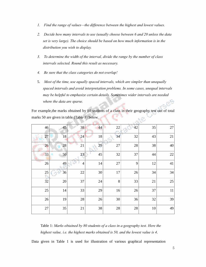
For example,the marks obtained by 80 students of a class in their geography test out of total

marks 50 are given in table (Table 1) below.

46 45 38 44 22 42 35 27

27 18 24 18 34 32 43 21

26 28 21 29 27 28 38 40

33 50 23 45 32 37 44 22

26 49 4 14 27 9 12 41

25 36 22 30 17 26 34 34

32 20 37 24 8 33 21 25

25 14 33 29 16 26 37 11

26 19 28 26 30 36 32 39

27 35 21 38 28 28 10 49

Table 1: Marks obtained by 80 students of a class in a geography test. Here the

highest value, i.e. the highest marks obtained is 50, and the lowest value is 4.

Data given in Table 1 is used for illustration of various graphical representation

6

methods. The data has to be organised before it can be used for convenient

representation.

Class interval

Frequency Cumulative frequency

Relative frequency (%)

Cumulative relative frequency (%)

1-5 1 1 1.25 1.25

6-10 3 4 3.75 5.00

11-15 4 8 5.00 10.00

16-20 6 14 7.50 17.50

21-25 13 27 16.25 33.75

26-30 20 47 25.00 58.75

31-35 12 59 15.00 73.75

36-40 10 69 12.50 86.25

41-45 7 76 8.75 95.00

46-50 4 80 5.00 100.00

Table 2: This is a frequency distribution table. The first column from the left

indicates the class intervals. Here, 1, 6, 11, 16, etc. are the lower class limits and

5,10,15,20, etc. are the upper class limits. The marks range from 1-50 and thus

have been divided into 10 class intervals with a class size of 5 each. The number

of values falling in each class interval has been written in the second column as

the frequency. Cumulative frequency values are obtained by adding the relative

frequencies in the respective row and all the preceding class intervals. Relative

frequency is obtained by dividing the respective frequency by the total frequency

(80, in this case). Cumulative relative frequency is also obtained in a similar way

as the cumulative frequency was obtained. This data can now be used for plotting

various types of graphs.

The whole data set is divided into ten classes with class interval of 5. The number of

values falling in each class interval is counted and is filled in as the frequency of the

respective class interval. With the frequency cumulative frequency, relative frequency

7

and cumulative relative frequencies are calculated. Table 2 shows the data and various

frequencies.

Figure 1 represents the data given in Table 1. The frequency distribution is plotted. The

x-axis shows the class intervals, and the y-axis indicates the frequency. The height of

the bars, therefore, shows the frequency.

Figure 1: Histogram representing data shown in above tables (Table 1 and 2).

The frequency distribution is plotted. The x-axis shows the class intervals and the

y-axis indicates the frequency. The height of the bars, therefore, shows the

frequency.

Frequency Polygons:

These are quite similar to frequency histograms. Here the frequency/ relative frequency is

plotted at the midpoint of the class interval instead of placing a bar across the width of a class

interval as in the frequency histogram. These points thus obtained are connected by straight

lines creating a polygonal shape and hence the name frequency polygon. So the x-axis

represents the mid-points of the class intervals, and the y-axis represents the frequency/

relative frequency (Figure 2).

Cumulative Frequency Polygon:

Here, it is similar to cumulative frequency histogram, where instead of drawing a bar across

1:5 6:10 11:15 16:20 21:25 26:30 31:35 36:40 41:45 46:500

5

10

15

20

25

8

the width of class interval, points are plotted at the height of cumulative frequency at the

midpoint of the respective class interval. These points are joined to form a cumulative

frequency polygon, also known as ogives. Similarly, cumulative relative frequency polygons

can also be made.

Figure 2: Frequency polygon representing data shown in Tables 1 and 2. The

frequency is plotted at the midpoint of the class interval instead of placing a bar

across the width of the class interval as in the frequency histogram. So the x-axis

represents the midpoints of the class interval, and the y-axis shows the frequency

of the respective class interval.

Figure 3 shows the cumulative frequency polygon representing data shown in Tables 1 and 2.

The cumulative frequency is plotted at the midpoint of the class interval. The cumulative

frequency is obtained by adding the relative frequencies in a particular row and all the

preceding class intervals. The x-axis represents the midpoints of the class interval, and the y-

axis shows the cumulative frequency at the respective class interval.

0 2.5 7.5 12.5 17.5 22.5 27.5 32.5 37.5 42.5 47.50

5

10

15

20

25

9

Stem and Leaf diagrams:

Stem and leaf diagram includes “stems” that represent the class intervals and “leaves” which

displays all the individual values. The advantage of stem and leaf diagrams over a histogram

is that the details are preserved even in the diagram, which are otherwise lost in constructing

a histogram. In histogram, frequencies are plotted, and the detail of individual values

contributing to the respective frequency is lost in the process, and therefore the original data

cannot be reconstructed from the histogram.

Figure 3: Cumulative frequency polygon/ Ogive representing data shown in

Tables 1 and 2. The cumulative frequency is plotted at the midpoint of the class

interval. The cumulative frequency is obtained by adding the relative frequencies

in a particular row and all the preceding class intervals. So the x-axis represents

the midpoints of the class interval, and the y-axis shows the cumulative frequency

at the respective class interval.

It can be demonstrated using data set of marks of 80 students in a geography test shown in

Table 1. The data ranged from 4 to 50, so we can make class groups based on the tens place

digit of each value 0, 1, 2, 3, 4 and 5, and the units place digits will form the leaves. If a

particular value is repeated in the data set, it has to be repeated in the leaf as many times as it

appears in the data set. Usually, the values on the leaf are arranged in increasing order. This

0 2.5 7.5 12.5 17.5 22.5 27.5 32.5 37.5 42.5 47.50

10

20

30

40

50

60

70

80

90

10

method includes and displays, each and every observation and no information is lost. It is

obvious from the method that the intervals with a higher number of values (frequency) placed

in it will have longer leaves and thus broad observations can be made in just a single glance.

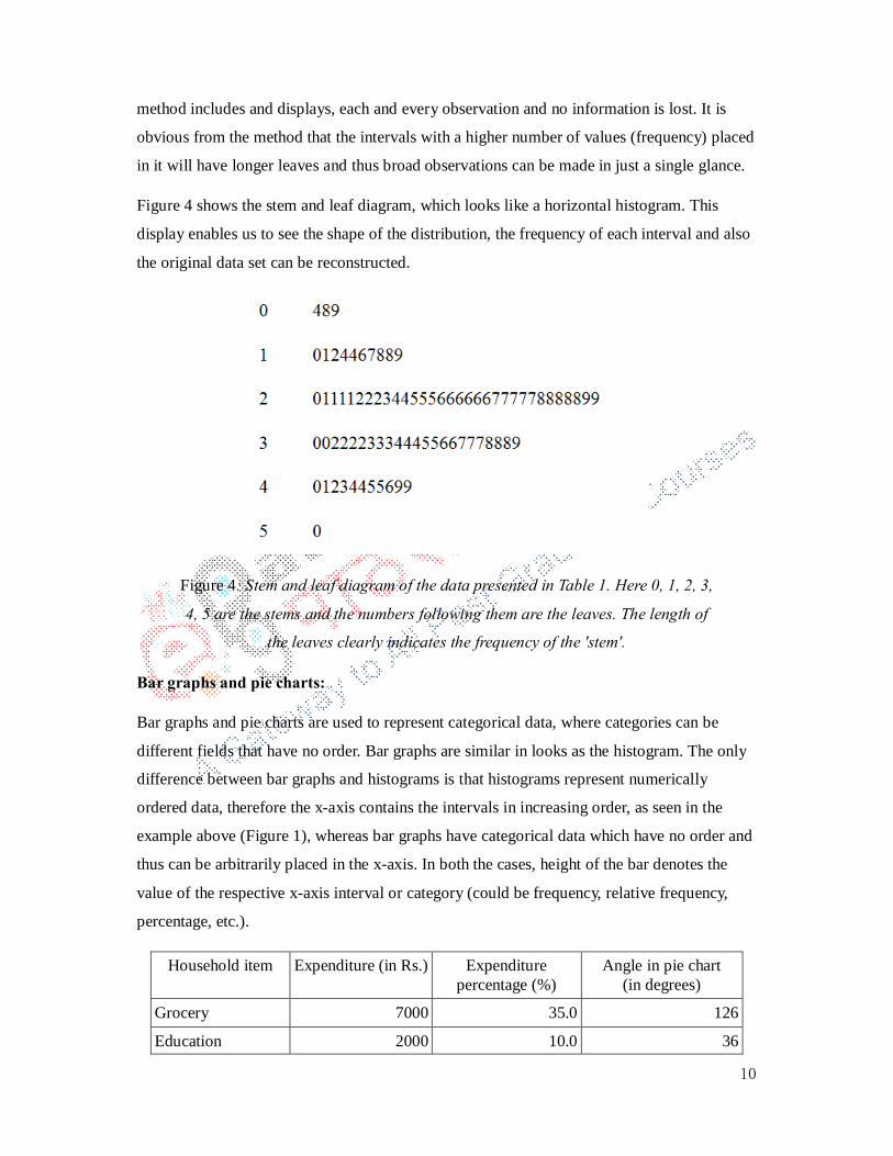
Figure 4 shows the stem and leaf diagram, which looks like a horizontal histogram. This

display enables us to see the shape of the distribution, the frequency of each interval and also

the original data set can be reconstructed.

Figure 4: Stem and leaf diagram of the data presented in Table 1. Here 0, 1, 2, 3,

4, 5 are the stems and the numbers following them are the leaves. The length of

the leaves clearly indicates the frequency of the 'stem'.

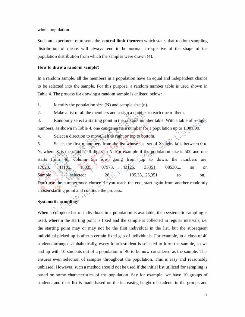
Bar graphs and pie charts:

Bar graphs and pie charts are used to represent categorical data, where categories can be

different fields that have no order. Bar graphs are similar in looks as the histogram. The only

difference between bar graphs and histograms is that histograms represent numerically

ordered data, therefore the x-axis contains the intervals in increasing order, as seen in the

example above (Figure 1), whereas bar graphs have categorical data which have no order and

thus can be arbitrarily placed in the x-axis. In both the cases, height of the bar denotes the

value of the respective x-axis interval or category (could be frequency, relative frequency,

percentage, etc.).

Household item Expenditure (in Rs.) Expenditure percentage (%)

Angle in pie chart (in degrees)

Grocery 7000 35.0 126

Education 2000 10.0 36

11

Travelling 1500 7.5 27

House Rent 5000 25.0 90

Entertainment 1000 5.0 18 Miscellaneous 3500 17.5 63

Total 20000 100.0 360

Table 3: List of expenses in a random household, where expenses are made in

heads: Grocery, Education, Travelling, House Rent, Entertainment and

Miscellaneous. Their percentage is calculated last and is followed by calculation

of their proportionate angle to be drawn in a pie chart.

Pie charts represent similar data as the bar graphs, however the categories are arranged

to form the circle (or pie) and their values (frequency, percentage, etc.) are made to

cover the area of the circle in for of sectors in a proportionate manner. The observation

values are converted to percentage form, and then their proportion is calculated, to

cover the total area of the circle, where each category occupies an area proportion to

their value. Table 3 shows the expenses incurred in a random household under different

heads. The amount is then represented as the percentage, followed by the calculation of

the angle that each of them would correspond to.

Figure 5: Bar graph representing the data given in Table 3. It is the

representationof expenses in a random household, where expenses are made in

GroceryEducation

TravellingHouse Rent

EntertainmentMiscellaneous

0

1000

2000

3000

4000

5000

6000

7000

8000

12

heads: Grocery, Education, Travelling, House Rent, Entertainment and

Miscellaneous. These are categories and can be put in any order without any

preference on the x-axis. The y-axis, i.e. the height of the bars indicates the

expense incurred under the respective head.

The bar graph in Figure 5 represents the data shown in Table 3. It is the representation of

expenses in a random household, where expenses are made in heads: Grocery, Education,

Travelling, House Rent, Entertainmentand Miscellaneous. Their percentage is calculated first

and is followed by calculation of their proportionate angle to be drawn in a pie chart (Figure

6).

Figure 6: Pie chart here represents the data shown in Table 3. It is the

representation of expenses in a random household, where expenses are made in

heads: Grocery, Education, Travelling, House Rent, Entertainment and

Miscellaneous. Their percentage is calculated first and is followed by calculation

of their proportionate angle to be drawn in a pie chart.

Research study designs:

With statistics, we aim to pursue systematic investigation to establish facts. Such

investigations may be destined to the discovery of new theories, establishment and

GroceryEducationTravellingHouse rentEntertainmentMiscellaneous

13

interpretation of facts, or revision of existing theories in the scenario of new facts available.

For such an investigation, it is mandatory to formulate a suitable study design so as to obtain

valid data to prove or disprove the hypothesis under study. Several study designs are used for

effectively carrying out experiments, the major ones are discussed below.

Types of studies: Studies can be broadly classified under two heads: Observational and

Experimental.

Observational: In observational studies, the researcher collects information about subjects

without applying any treatments to the subject, just by observation. This includes cross-

sectional, correlational, case-control, case reports, retrospective and prospective studies

Experimental: In experimental studies, the researcher deliberately introduces interventions

and investigates the impact of the intervention

Another way of classifying research study design is based on the period for which the data is

collected, and this includes prospective and retrospective study design.

Prospective: In prospective studies, the data are collected as a part of the study, i.e., the

current data is obtained starting from the date, when the study formally begins. For

example,experiments&survival studies.

In this case, effect of certain interventions on the subjects can be studied, by giving proper

instructions/ treatments, etc. to the subjects.

Retrospective: In retrospective studies, the data refer to past events and is acquired from

existing sources by personal interviews, surveys, official records (hospital records, bank

records, etc.). For example, case-control studies.

No specific combinations can be studied, and data is restricted to the events which have

already taken place, and hence no modification in subjects' conditions can be made, for

further analysis. Retrospective studies usually consume lesser time that prospective studies

and is also cheap to obtain. The data obtained may be inaccurate by the virtue of recall errors.

Research study designs are also sometimes classified as longitudinal and cross-sectional

studies depending on the investigation conducted.

Longitudinal: In longitudinal studies, the researcher investigates the changes in the same

subject as the time passes. For example, survival studies.

Cross-sectional: In cross-sectional studies, the researcher investigates the individuals only

14

once at a suitable point.

Observational studies:

1. Case reports and case series:

It includes detailed, critical study of a single case (case-report) or a set of similar cases (case-

series), for a specific characteristic (diseased condition, treatment, intervention, etc.). The

scientific evidence from such studies are considered weak and thus can be used for making

hypotheses bout the cause/ effect, etc. of the respective characteristic and not for establishing

facts/ outcomes.

2. Cross-sectional survey:

All information is collected at the same time and indicates the scenario in that period. These

studies results in the frequency of interested characteristics (disease, physiological condition,

drug impact, etc.) in the population. The outcomes obtained from these studies can only be

used to make hypotheses and not for validating a statement. However, sampling always

remains an issue for these studies. Further, the results suffer from bias due to non-response or

volunteer response.

3. Case-control study:

These studies obtain information from case subjects (who are known to have the

characteristics under study for example a diseased person) and from control subjects (who do

not exhibit the characteristics under study, for example, a normal person). This information is

used to test the statement under scrutiny. For example, to test the theories about disease

occurrence, information is collected from diseased individuals and normal individuals (not

suffering from the disease under study). A retrospective study is conducted, and the results

are analysed.

4. Cohort study:

A group of subjects is identified, who have or are expected to have characteristics under

study. Such groups from a population are called as cohorts. These cohorts are formed into a

group based on differential patterns exhibited for a given characteristic. These studies may be

prospective or retrospective, but mostly prospective studies are preferred, where the cohorts

are observed over a period (longitudinal) to establish facts about the characteristic under

study. The advantage with prospective cohort study is that the quality and depth of data can

15

be controlled as per the requirements of the study. However, selection of subjects and

formation of cohorts is a critical task. It is concerned with the prevalence of a particular

characteristic in a population and is, therefore, also known as prevalence study.

Experimental studies:

1. Community trials:

“Community trials also called community intervention studies, are (mostly preventive)

experimental studies with whole communities (such as cities or states) as experimental units;

that is, interventions are assigned to all members in each of a number of communities. These

are to be distinguished from field trials where interventions are assigned to healthy

individuals in the community and from clinical trials in which interventions are assigned to

patients in a clinical setting. Except for the experimental unit, the conduct of controlled

community trials follow the same procedures as controlled clinical trials, including the

requirement of informed consent of the communities meeting the eligibility criteria (e.g.,

consent being given by city mayors or state governors), randomization to treatment and

control groups, and follow-up and measurement of endpoints” (6). However, consent from

individual subjects is not required, and it is possible that an individual may not even know

that are part of a community study. But it is required that the researcher in this case ensures

that the treatment or study is ethical and possess no harm to the subjects.

2. Clinical trials:

In the Encyclopaedia of Biopharmaceutical Statistics by Chow (2000) (7), a clinical trial is

defined as “....an experiment performed by a health care organization or professional to

evaluate the effect of an intervention or treatment against a control in a clinical environment.

It is a prospective study to identify outcome measures that are influenced by the intervention.

A clinical trial is designed to maintain health, prevent diseases, or treat diseased subjects.

The safety, efficacy, pharmacological, pharmacokinetic, quality-of-life, health economics, or

biochemical effects are measured in a clinical trial”. Clinical trials are conducted to

demonstrate the safety and effectiveness of new drugs/ products to the FDA. They are

conducted on individuals suffering from the target disease. It is mandatory that the

individuals must be informed about the benefits and risks involved in the trial and appropriate

formal consent be taken. Randomized controlled clinical trials are most commonly practised

method for clinical trials. The subjects are randomly grouped to form treatment and control

16

sets. Occasionally, if control groups are unavailable, historical control groups are also used,

but this approach compromise on the efficiency and confidence of the outcomes obtained.

Investigators are usually blinded to avoid external bias on the data collected from treatment

and control group. Sometimes both subject and the investigator are blinded, and it is called as

double blinded.

Need for sampling

Data collection and processing may prove cumbersome if the size of the population exceeds a

threshold value. To deal with such a situation where collecting information from a large

population is resource consuming or impossible, statisticians resort to collect information

from a critically selected sample from the population under study. The results obtained from

such samples are then extended to acquire accurate statistical estimates of population

parameters. However, selecting sufficiently large samples result in more accurate statistical

inference. A critical part of such an analysis is choosing samples appropriately and efficiently.

Since inappropriately chosen samples may lead to incorrect inferences, it is imperative to

select the correct method for drawing a sample out of a population. The ultimate goal of

sampling is to choose a miniature representative of the population.

Such a sampling may be done in several ways which vary from case to case basis. Depending

on several factors, different methods of sampling may be used, and the decision has to be

made critically.

Types of sampling

Simple Random sampling:

It is one of the simplest and most convenient methods to obtain reliable information about a

population, and it ensures unbiased estimates of population to an extent. The basic principle

behind the method is to choose randomly a sample of size n from a given population under

study of size N. It is obvious from the method that every object in the population has equal

probability of being included in the sample.

For example, you have a set of 90 balls of bingo, and you draw five of them and record the

numbers on them. Repeat this procedure for 20 times, then the numbers recorded every time

would be different from every other time. Further, if you calculate the mean of the numbers

drawn in every set, the mean would be different, but if these means are plotted, it will result

in a normal distribution. Thus in each set the randomly selected balls, broadly represents the

17

whole population.

Such an experiment represents the central limit theorem which states that random sampling

distribution of means will always tend to be normal, irrespective of the shape of the

population distribution from which the samples were drawn (4).

How to draw a random sample?

In a random sample, all the members in a population have an equal and independent chance

to be selected into the sample. For this purpose, a random number table is used shown in

Table 4. The process for drawing a random sample is enlisted below:

1. Identify the population size (N) and sample size (n).

2. Make a list of all the members and assign a number to each one of them.

3. Randomly select a starting point in the random number table. With a table of 5-digit

numbers, as shown in Table 4, one can generate a number for a population up to 1,00,000.

4. Select a direction to move, left to right or top to bottom.

5. Select the first n numbers from the list whose last set of X digits falls between 0 to

N, where X is the number of digits in N. For example if the population size is 500 and one

starts from 4th column 5th row, going from top to down, the numbers are:

17028, 41105, 16035, 07973, 43125, 35351, 08530.... so on

Sample selected: 28, 105,35,125,351 so on...

Don't use the number once chosen. If you reach the end, start again from another randomly

chosen starting point and continue the process.

Systematic sampling:

When a complete list of individuals in a population is available, then systematic sampling is

used, wherein the starting point is fixed and the sample is collected in regular intervals, i.e.

the starting point may or may not be the first individual in the list, but the subsequent

individual picked up is after a certain fixed gap of individuals. For example, in a class of 40

students arranged alphabetically, every fourth student is selected to form the sample, so we

end up with 10 students out of a population of 40 to be now considered as the sample. This

ensures even selection of samples throughout the population. This is easy and reasonably

unbiased. However, such a method should not be used if the initial list utilized for sampling is

based on some characteristics of the population. Say for example, we have 10 groups of

students and their list is made based on the increasing height of students in the groups and

18

suppose we select only the first student from each group so as to have a sample of 10. If with

such a sample we study the weight of the students in that age group, then this is likely to be

incorrect as we have selected the shortest from all the groups.

Convenience sampling:

Here the samples are selected based on the availability and ease of carrying out data

collection. Although they may be considered as the representative of the population from

where they have been collected, there is no assurance that it covers all types of characteristics

otherwise present in the population. They are still used in cases where random sampling is

impossible. Such results are descriptive and may help in deciding a future course of action,

but they should not be used to obtain a general view about the population under study, since

they are likely to be biased. Convenience sampling is used for preliminary studies.

Stratified random sampling:

As the name suggests, this is a modified version of simple random sampling where the

sample is picked up in equal proportions from all the strata (subgroup or collection) of the

population under study. This is used when the data is not constant across the population, and

there are known sub-groups or collections of individuals present. This helps in improving the

efficiency and accuracy of sample estimates. The method used is very simple, where the

population is divided into subgroups based on some known characteristics, and then a simple

random sample is collected from each subgroup. Stratified random sampling provides an

edge over simple random sampling produces an unbiased estimate of the population mean

with better precision for the same sample size n. The sample collected from each subgroup

can be varied depending on the variability exhibited by the subgroup to further improve on

the precision.

19

Col/Row 1 2 3 4 5 6 7 8 9 10

1 00439 60176 48503 14559 18274 45809 09748 19716 15081 84704

2 29676 37909 95673 66757 04164 94000 19939 55374 26109 58722

3 69386 71708 88608 67251 22512 00169 02887 84072 91832 97489

4 68381 61725 49122 75836 15368 52551 58711 43014 95376 57402

5 69158 38683 41374 17028 09304 10834 10332 07534 79067 27126

6 00858 04352 17833 41105 46569 90109 32335 65895 64362 01431

7 86972 51707 58242 16035 94887 83510 53124 85750 98015 00038

8 30606 45225 30161 07973 03034 82983 61369 65913 65478 62319

9 93864 49044 57169 43125 11703 87009 06219 28040 10050 05974

10 61937 90217 56708 35351 60820 90729 28489 88186 74006 18320

11 94551 69538 52924 08530 79302 34981 60530 96317 29918 16918

12 79385 49498 48569 57888 70564 17660 68930 39693 87372 09600

13 86232 01398 50258 22868 71052 10127 48729 67613 59400 65886

14 04912 01051 33687 03296 17112 23843 16796 22332 91570 47197

15 15455 88237 91026 36454 18765 97891 11022 98774 00321 10386

16 88430 09861 45098 66176 59598 98527 11059 31626 10798 50313

17 48849 11583 63654 55670 89474 75232 14186 52377 19129 67166

18 33659 59617 40920 30295 07463 79923 83393 77120 38862 75503

19 60198 41729 19897 04805 09351 76734 24057 87776 36947 88618

20 55868 53145 66232 52007 81206 89543 66226 45709 37114 78075

21 22011 71396 95174 43043 68304 36773 83931 43631 50995 68130

22 90301 54934 08008 00565 67790 84760 82229 64147 28031 11609

23 07586 90936 21021 54066 87281 63574 41155 01740 29025 19909

20

24 09973 76136 87904 54419 34370 75071 56201 16768 61934 12083

25 59750 42528 19864 31595 72097 17005 24682 43560 74423 59197

26 74492 19327 17812 63897 65708 07709 13817 95943 07909 75504

27 69042 57646 38606 30549 34351 21432 50312 10566 43842 70046

28 16054 32268 29828 73413 53819 39324 13581 71841 94894 64223

29 17930 78622 70578 23048 73730 73507 69602 77174 32593 45565

30 46812 93896 65639 73905 45396 71653 01490 33674 16888 53434

31 04590 07459 04096 15216 56633 69845 85550 15141 56349 56117

32 99618 63788 86396 37564 12962 96090 70358 23378 63441 36828

33 34545 32273 45427 30693 49369 27427 28362 17307 45092 08302

34 04337 00565 27718 67942 19284 69126 51649 03469 88009 41916

35 73810 70135 72055 90111 71202 08210 76424 66364 63081 37784

Table 4: Random number Table

Cluster Sampling:

The population under study is divided into groups or clusters as the name suggests. Some of

these clusters are selected based on the availability of their member details. Observations are

collected either from all the members of the clusters or if the numbers arevast, and then the

members are selected based on simple random sampling. Cluster sampling is used when

selecting simple random samples results in members of the sample being widely scattered

such that the data collection becomes tedious and expensive. Such a technique is more

practical, economical and convenient than simple/ stratified random sampling. However, the

result obtained may not be as unbiased as the random sampling technique but is compensated

by the resources saved in the process. For example, a survey has to be conducted in a city to

find out the most visited shopping mall. Selecting random samples across the city would

prove to be quite time consuming and expensive. So in order to save on resources, certain

localities are selected, and either the data is collected from all the individuals of the locality

or by taking a simple random sample.

Critical care has to be taken while deciding on sampling technique to be used for a study.

21

Sampling Error: The difference between thetrue population result and asample result is

called as the sampling error and is caused due to chance sample fluctuations

Non-Sampling Error: Sample data that are incorrectly collected, recorded, or analysed (such

as error due to a defective instrument, a biased sample or manual errors in data handling).

Measures of central tendency:

As the name suggests, this includes methods for calculating the tendency of localization of

thecenter of the data distribution. Measures of central tendency include arithmetic mean,

mode, median, geometric mean and harmonic mean, also known measures of location. A

measure of central tendency gives us an idea about the location where maximum number of

observations are expected to be located, whereas measures of dispersion gives us an idea

about the spread of observations in a distribution.

The three most popularly used measures of central tendencies are mean, mode and median.

Mean: Also known as arithmetic mean or average. It is the sum of the individual values in a data set

divided by the total number of values present in the data set. Mean gives the arithmetic

average of all the observed values of the population or the sample under study. Mean

calculated for the population is denoted as μ, where sum of individual values obtained from

the entire X. To obtain the mean of a population, sum of all the individual observation values

is divided by the population size, N. For calculating sample mean the sum of individual

observation values in the sample is taken and divided by the sample size, n.

Formula: Sample mean: X̄ = ∑ xn

Population mean: μ = ∑ xN

Mean is the most commonly used method to measure central tendency. Since all the values

are taken into consideration while calculating mean, the extreme values sometimes pose a

problem. In such a case where a couple of extreme values are present in the data, shift the

central location, and the outcome is no more the representative of the location of the great

majority of observation values. For example, for a set of ten babies born on a particular day

in a hospital whose birth weights are given in Table 5.

22

Baby Birth weight-1 (in grams)

Birth weight-2 (in grams)

1 3278 527

2 2845 2845

3 3567 3567

4 3290 3290

5 4167 4167

6 3890 3890

7 3675 3675

8 3178 3178

9 3980 3980

10 3321 3321

Table 5: The birth weights of ten babies born in a single day in a hospital.

Mean = sum of individual values/total number of values

= (3278+2845+3567+3290+4167+3890+3675+3178+3980+3321)/10 = 3519.1

The mean the given data set is 3519.1 grams, where five values out of ten are below the

mean, and five are above the mean.

Suppose, the first baby was born premature with a birth weight of 527grams, then the mean

would be 3244.0 grams, and now, out of ten only two values are less than the mean and eight

are above the mean. Whereas mean was quite apt for the first case, in the second case with

one extreme value, mean was proved to be a poor measure of central tendency. Mean gives

equal weight to all values. However, extreme values must be removed with appropriate

justification.

Median: The next widely used measure for central tendency is median or sample median. It is the

central observation value in the data set, which when arranged in ascending order has an

equal number of observations below and above it. This is more accurate in case of a sample

or population with an odd number of observations. For a data set with even number of

observations, the average of two central values is taken as the median.

Formula: The observations in thedata set are first arranged in ascending order.

23

If number of observations (n) is odd: Median = (n+1)

2

th

term.

If the number of observations (n) is even: Median = Average of thn

2and th+n 1

2term.

The formula used is different for data sets with odd and even number of observations because

there is no unique central point in case of data set with even number of observation, therefore

when the average is taken, the purpose of having equal number of observations below and

above the median is still fulfilled.

Example: Calculating median for data set in Table 5.

Step 1: Arrange the given data points in ascending order:

2845 3178 3278 3290 3321 3567 3675 3890 3980 4167

Step 2: Since n=10, take an average of 5th and 6th values in the data set: (3321+3567)/2=

3444.

Median= 3444.

Median is the preferred measure of central tendency when the data is non-numeric. For

example, grades of ten students in an exam.

Association of Mean and Median:

The comparison of Mean and Median can give an insight into the type of distribution

displayed by the data set. For a symmetric distribution, mean and median are expected to

have approximately the same value. However, for a skewed distribution, mean and median,

together indicate the inclination of the distribution. For a negatively skewed (skewed to the

left) distribution,the arithmetic mean tends to be smaller than the median. Similarly for a

positively skewed (skewed to the right) distribution the arithmetic mean tends to be larger

than the median, since there are number of observations in the second half of the curve.

Mode:

For a large discrete data set, mode is used as a measure for central tendency. Mode is the

most frequently occurring value among all the observations in a sample/ population. So for

Table 5 shown above there is no mode as all the values occur exactly once.

Whereas some other distributions may have more than one mode i.e. more than one value

from the data set has the same highest frequency of occurrence. This is also sometimes used

as a mode to characterize a distribution, by the number of modes present in the distribution. A

24

distribution with one mode is called unimodal, two modes-bimodal, three modes-trimodal,

and so on and so forth.

Geometric Mean:

The product of all the values in a data set, followed by taking their nth root gives the

geometric mean. Since a product is taken, it is mandatory that all the values in the data set

must be greater than 1.

For a data set where several values are much higher/lower than the rest of the values,

geometric mean is preferred over arithmetic mean. Because using an arithmetic mean in such

a case would distort the mean. When the sample values that do not conform to a normal

distribution, it is preferred to use the geometric mean.

Geometric mean = (a1* a2* a3*….an)1/n , where a1, a2,… an are the observation values and n is

the number of observations.

The Geometric Mean is the arithmetic mean of the data after transforming them to a log scale

because on the log scale the data become symmetric. So depending on the distribution pattern

of data set, geometric mean can be used for more appropriate measure of central tendency.

For example, in the Table 5 for birth weight (birth weight-2), the geometric mean is found to

be 3497.46. The mean for the same data set was calculated to be 3244.0 grams. Therefore, if

we see the number of values below and above the calculated mean, geometric mean is seen as

a better measure of central tendency, with five values above it and five values below.

Harmonic Mean:

The reciprocal of the arithmetic average of the reciprocals of the original observations gives

the harmonic mean.

For a data set with few extreme outliers, an arithmetic mean may prove to be misleading, in

such a case harmonic mean comes out as the most appropriate method. It gives less

importance to extreme outliers and thus provides a more accurate picture of the average.

Formula for harmonic mean:

n21 a1...

a1

a1

nH+++

= , where H is the harmonic mean, a1, a2, …, an are the observation

values and n is the number of observations.

25

For example, Table 5 where we calculated the mean with one outlier of premature birth

weight (birth weight-2), the mean was calculated to be 3244.0 gms. The harmonic mean for

this data set is 3475.78, and here there are five values are less than the mean and five are

more than the mean, this portrays a better picture of central tendency.

Harmonic mean is less biased due to the presence of few outliers and is best to use when

majority of the values in the population are distributed uniformly but where there are a few

outliers within significantly higher values.

Measures of Dispersion:

Sometimes, two normal distributions may have identical measure of central tendency, i.e.,

same mean, mode and median. However, this doesn't necessarily imply that the two

distributions are identical. This indicates that three measures of central tendency alone stand

inadequate to describe any normal distribution. Variability is usually observed during

measurement of data set. Sources of such variability can be categorized as biological,

temporal and measurement.

Biological variations arise by the virtue of various factors that influence biological

characteristics, which most commonly include age, sex, genetic factors, dietand socio-

economic environment. There are several examples that can illustrate this point. Several

human body characteristics vary with age, say, basic metabolic rate, blood pressure, body

weight, and so are their average values.

Temporal variations include time-related changes, for example, temperature, climate,

agricultural produce, etc. One such example is temperature variation during day and night.

Another important source of variation is measurement errors. The differences between the

true value of a variable and the measured/ reported value are called measurement errors.

Measurement errors form an important area of study in statistics.

For the measurement of dispersion several measures have been developed, termed as,

measures of dispersion, to describe the variability observed in the data set. Major measures

include the range, the mean absolute deviation, and the standard deviation. Dispersion

together with central tendency constitutes the most widely used properties of distributions.

Dispersion measurement illustrates the similarity between two sets of values. The lower the

measure of dispersion, the more is the similarity between two sets, and a larger value of

26

dispersion indicates a more widely distributed set of values

There are three main measures of dispersion:

Range: Range is the simplest way to measure the dispersion; it is the difference between the lowest

and the highest value in the distribution set. To calculate the range, we need to locate the

lowest and the highest values. This task is easy when we are handling small number of values

but for a larger data set, the ideal way is to sort them in ascending or descending order.

For example, look at the two given data sets;

Data set 1:X= 4,7,3,8,12,56,78,34,45,77

Data set 2: Y= 4, 7,3,8,12,56,78,34,45,770

Xh= 78; Xl= 3; Yh= 770; Yl= 3, where h and l indicate the highest and the lowest values of the

respective data set.

So, Range for X= Xh-Xl= 78-3=75

Whereas, range for Y = Yh- Yl =770-3=767

But as the data sets suggests here, with only one different entry the range changes drastically

and therefore a range is not a preferred measure of dispersion. Moreover, since the range is

only affected by the two extreme end values, it doesn't justify the intermediate values, and

two very different sets may have the same range.

For example, data set 1: 1,2,4,5,6,7,9,10,11,13

Data set 2: 1,1,1,1,1,1,1,1,1,13, here the range is same for both data sets.

Range is used only for a very preliminary idea about the two data sets or for ordinal data and

is very rarely used for sophisticated high-end studies.

Mean Absolute Deviation:

The second way of calculating variability is the mean absolute deviation from mean. The

name itself suggests the protocol for its calculation, i.e., first the mean of the observation is

calculated and then the deviation of each observation from the mean is calculated. Then the

absolute value of each deviation is taken, and the mean of these values give the mean

absolute deviation. So the steps for calculating the mean absolute deviation are:

27

Calculate mean of the given set of observations

Calculate deviation of each observation from the mean value, (also called as the

deviation score) and take their absolute value.

Calculate the mean of these absolute deviation values obtained.

Example: Calculation of mean absolute deviation for a given data set

Data set: X= 45, 35, 65, 75, 95, 25

Mean: (45+55+65+75+95+25)/6 = 60

Absolute deviation: 15, 5, 5, 15, 35, 35

Mean of absolute deviation: (15+5+5+15+35+35)/6= 18.33

The formula for calculating mean absolute deviation can be written as:

Mean Absolute deviation: �|����|

�

whereXi= observation value,

�= mean of the observation values

n= total number of observations

Population Variance and Standard Deviation:

With the advancement in computational approaches, interrelated measures of variance and

standard deviation are frequently used these days. Both variance and standard deviation use

squared deviation about the mean instead of absolute value of the deviation as in mean

absolute deviation method.

Variance calculation involves the use of deviation scores. It is the mean of the squares of

deviation scores of all the observations in a given distribution. Therefore, the step for

calculating variance can be given as:

Calculating deviation score for each observation

Calculating squares of these deviation scores

Calculatingmean of these squared deviation scores

Variance is symbolized as σ2 for a population and by s2 for a sample. It can be understood

with a simple relation with the mean, i.e., the larger the variance, the more is the variation

among the scores. The smaller the variance is, the less is the deviation in the scores, on

average, from the mean. While calculating variance, a computational formula is often

28

used,this is algebraically equivalent to the formula given below:

Formula:( )

NμX

=σ i∑ − 22 , where N is the total number of elements present in the

population.

Standard Deviation: Although variance is a good approach for use as a measure of

dispersion, but since it is the outcome of squared terms, it is expressed in squared units of

measurement, which limits its usefulness as a descriptive term. It can be tackled by using

standard deviation, which is the square root of the variance and is, therefore, expressed in the

same units of measurements. Standard deviation also indicates the shape of the distribution of

values. Distribution with smaller standard deviation is narrower than those with larger

standard deviation.

Formula:� = ��(����)� �

Sample Variance and Standard Deviation:Sample variance takes a slightly modified

formula than that used for the population variance. Sample variance is indicated using s2 and

sample standard deviation is denoted as s. For a sample size of n, and mean X the formulae

used for calculating sample variance and standard deviation are indicated below:

Formula: Sample variance: ( )

1

22

−

−∑n

XX=S i

Sample standard deviation: ( )

1

2

−

−∑n

XX=S i

Semi-Interquartile Range:For a given data set, the valueswhich divide the data into four

equal parts are called quartiles. We have seen that the median divides the data set into two

equal parts, lower half and upper half. Now the median of the lower half of the data set forms

the lower quartile, represented as Q1. Similarly, the median of the upper half of the data set

forms the upper quartile, represented as Q3. The median of the complete data set is Q2. So

we have three values, Q1, Q2 and Q3, which divides the data set into four equal parts.

For example, we have the following data set,

12, 16, 17,21, 23, 25, 29,31, 32, 35

the median of the above data set: Since there are even number of observations,

Median = (23+25)/2 = 24;

29

Lower half: 12, 16, 17, 21, 23

Median for the lower half, first quartile or Q1 = 17

Upper half: 25, 29, 31, 32, 35

Median for the upper half, third quartile or Q3 = 31

The interquartile range is defined as the difference between third and first quartile.

The semi-interquartile range (or SIR) is defined as the difference of the third and first

quartiles divided by two. Therefore, semi-interquartile range (SIR), is given as,

SIR = (Q3-Q1 )/ 2

Use of SIR is preferred in case of skewed data as it doesn't take extreme values into account

and at the same time takes into account a wide range of the intermediate values.

So for the data presented above,

Semi-interquartile range = (Q3-Q1)/ 2

= (31-17)/ 2

= 14/ 2 = 7

PROBABILITY

Basic definitions in probability study:

Event: An event can be defined as a collection of results or outcomes of a procedure.

Simple event: An event which can't be further subdivided onto simpler modules.

Independent Events: In a given case of two events A and B, where the occurrence of one

does not affect the occurrence of the other, the two events can be termed as independent.

Sample space: It consists of all possible simple events, i.e. all expected outcomes that can't

be further broken down.

Probability is usually denoted as P and individual events are symbolized as A, B, C, etc.

So, P (A) = Probability of event A.

Basic Rules for Computing Probability

Rule 1: Relative Frequency Approximation of Probability

When a given procedure is repeated a large number of times and the number of times event A

occurs is enumerated, then based on these results, P (A) is estimated as follows:

30

����=��� ��� �� ��� �� � ��������

����� ��� ��� �� ������

Rule 2: Classical Approach to Probability

This approach is used if a given procedure has n different simple events and it is known that

the occurrence of each of those simple events is equally likely. If event A can occur anumber

of time of these n ways, then

����=��� ��� �� ���� � ��� �����

��� ��� �� ��������� ��� ��� ������

Rule 3: Subjective Probabilities

Here, the probability of event A, P (A),can be estimated based on the prior information of the

relevant circumstances.

Law of Large Numbers: When a given procedure is repeated multiple times, the probability

calculated using Rule 1 in this case approaches close to the actual probability.

For example, in your class there are 15 students; one student has to be selected randomly.

Since there is no preference everyone has an equal chance of being selected. In this what is

the probability that you will be selected?

In such a situation classical approach(Rule 2) is used, all the 15 students have an equal

chance to be selected.

( )151

srofoutcometotalnumbeomepectedoutcnumberofexselectionP ==

Limits of Probability:

The probability of an event that is impossible is 0, and the probability of an event that is

certain to occur is 1. For any event A, the probability, therefore, will be in the range of 0 to 1.

For any event A, 0 <P (A) < 1. So for a given even if P is found to be 0.5, this indicates a 50%

chance, if it exceeds 0.5, the event is likely to happen whereas if P is less than 0.5, then the

event is unlikely to happen, however it is not impossible, it is just a matter of chance.

Complementary events:

The complement of event A, denoted by�, includes all outcomes in which the event A does

not occur.

31

As in the example above, P (not selection) = P (���������) = 14/15.

Here P(A) and P(�) are mutually exclusive. So each simple event can be classified as either A

or�. Addition of such a set of complementary events is always 1, because for a simple event,

either it will happen or it will not happen. As in the example showed above, you will be either

selected or not selected and no other outcome is possible. So, it can be written as, P(A) +

P(�) =1, also,

P(A) = 1 – P(�) and,

P(�) = 1 - P(A)

Probability addition rule:

Any event combining two or more simple events is known as compound event. So if we

consider two simple events, A and B, the compound event would be neither event A or B

occurring or either A nor B occurring or two events A and B occurring together.

General Rule for a Compound Event: When finding the probability of occurrence of event

A or event B, the total number of ways A can occur and the number of ways B can occur is

calculated, in such a way that none of the outcomes is counted more than once.

Figure 7: This figure indicates the addition rule for a compound event, which is a

combination of two events, A and B. The addition rule varies depending on

whether the two events are disjoint or not. Disjoint events cannot happen at the

same time. They are separate, non-overlapping events, i.e. they are mutually

exclusive. So, when the two events are disjoint the two probabilities can be

directly added to obtain the combined probability. On the other hand if the two

events are not disjoint then the two individual probabilities of event A and B are

added and the probability of overlapping events is subtracted from the sum to

obtain the combined probability of the two events, so as to avoid counting the

same outcome twice.

32

Classification of compound events:

The compound events can be classified depending on the occurrence of the event, for a set of

two events, A and B, there can be three possibilities and each one has a different probability

rule and are explained as Venn diagrams.

1. Events cannot occur together at the same time: Mutually exclusive

Two events, A and B, are said to be mutually exclusive if the occurrence of one event

precludes the occurrence of other, i.e. A and B can never occur simultaneously.

For example, in a deck of cards, what is the probability of getting an ace and a king when one

card is selected? None. Because these two events are mutually exclusive and if one card is

drawn, there can be only one of these as an outcome, either ace or king. The Venn diagram in

such a case would look like the one in Figure 8a.

Addition rule to find out the probability that either of the two events will take place is a

simple addition process, since the two events are mutually exclusive and non-overlapping.

So the probability that either of the two will occur, can be written as P(A or B) and the

individual event probabilities can be written as P(A) and P(B), then

P (A or B) = P (A) + P (B)

For example, what is the probability of getting an ace or a king from the roll of the deck?

P(ace) = total number of aces/ total number of cards in the deck

( )

( )

( )528

524

524aceorkingP

524

rofcardstotalnumberofkingstotalnumbekingP

524

rofcardstotalnumberofacestotalnumbeaceP

=+=

==

==

2. Both events can occur together or individually one at a time: Union or A U B

Two events are said to be in union (indicated with symbol 'U' in between) when for two

events, A and B, either A occurs or B occurs or both occur. The Venn diagram in such a case

would look like the one in Figure 8b.

For example, in a deck of cards, the probability of getting an ace or a club, when one card is

taken. In such a case, when the sample space is 52, a card drawn can be an ace (4 of 52), can

be a club (13 of 52), can be both (1 of 52) or any other card.

Addition rule to find out the probability of such an event (non-mutually exclusive) where the

probability that either of the two (A or B) will occur, can be written as P(A or B) and the

33

individual event probabilities can be written as P(A) and P(B), then

P(A or B) = P(A) + P(B) – P (A and B)

With this formula, when we solve the above problem of club and ace, we get

P (Ace or Club) = P(Ace) + P(Club) − P(Ace and Club)

P (Ace or Club) = 452

+ 1352

− 152

= 1652

Figure 7 indicates the condition and the rules for these two cases whether the two events are

disjoint or not.

3. Both events A and B occurring at the same time: Intersection or A∩ B.

Two events are said to be in an intersection (indicated with a symbol '∩' in between) when

two events, A and B, occur at the same time, i.e. they intersect. This is also known as the joint

probability. The Venn diagram in such a case would look like the one in Figure 8c.

For example, in a deck of cards, the probability of getting an ace and club when one card is

taken. As seen in the above example, when the sample space is 52, a card drawn can be an

ace (4 of 52), can be a club (13 of 52), can be both (1 of 52) or any other card.

In calculating probability in this case, multiplication rule is used, where probability of

intersection for two independent simple events, A and B, is given as P(A and B) the

individual event probabilities can be written as P(A) and P(B), then

P(A ∩ B) = P(A) * P(B)

With this formula, the above problem can be solved

P (Ace and club ) = P(Ace) ∗P(club )

P (ace) = total number of acestotal number of cards

= 452

P (club) = total number of clubstotal number of cards

= 1352

P (aceor king) = 452

∗1352

= 152

Differentiating independent events and mutually exclusive events: independent events and

mutually exclusive events are usually confused as same; however they are two different

concepts and are defined in terms of intersection. For two independent events, A and B,

where P(A) and P(B) are probabilities of individual events respectively,

P(A) > 0 and P(B) > 0, so

P (A∩B) = P(A) * P(B) > 0. Therefore, when P (A∩B) is not equal to 0, which means there is

34

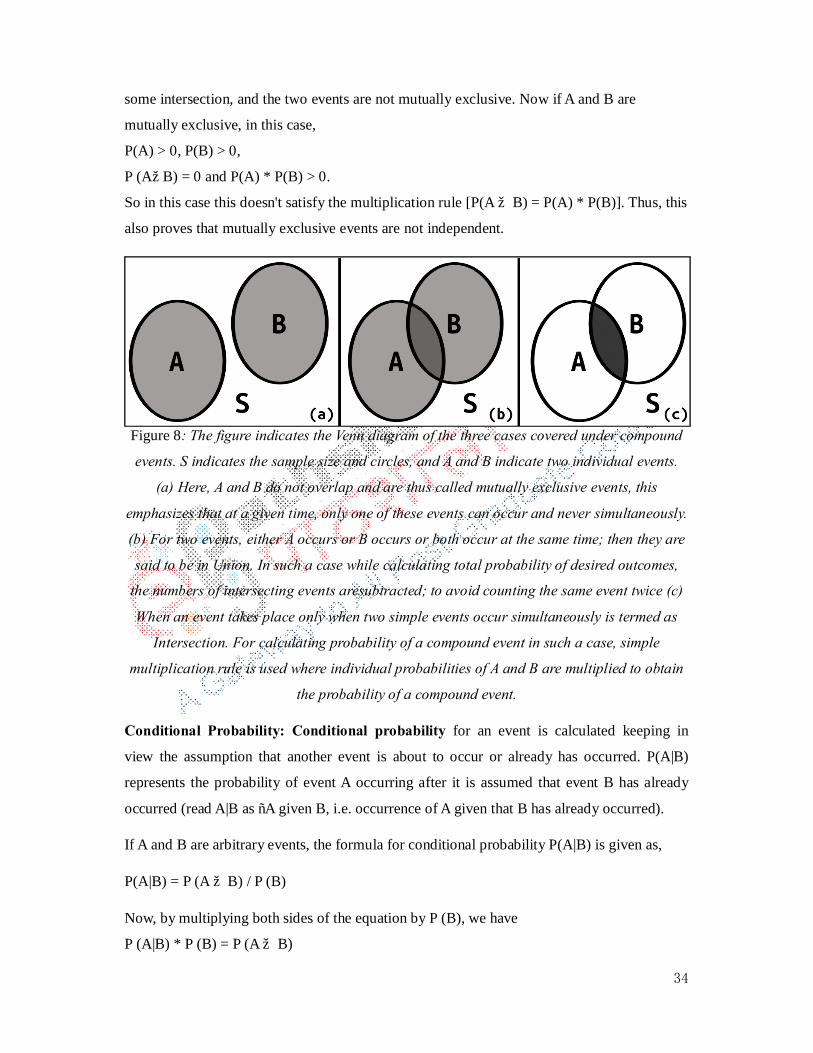
some intersection, and the two events are not mutually exclusive. Now if A and B are

mutually exclusive, in this case,

P(A) > 0, P(B) > 0,

P (A∩B) = 0 and P(A) * P(B) > 0.

So in this case this doesn't satisfy the multiplication rule [P(A ∩ B) = P(A) * P(B)]. Thus, this

also proves that mutually exclusive events are not independent.

Figure 8: The figure indicates the Venn diagram of the three cases covered under compound

events. S indicates the sample size and circles, and A and B indicate two individual events.

(a) Here, A and B do not overlap and are thus called mutually exclusive events, this

emphasizes that at a given time, only one of these events can occur and never simultaneously.

(b) For two events, either A occurs or B occurs or both occur at the same time; then they are

said to be in Union. In such a case while calculating total probability of desired outcomes,

the numbers of intersecting events aresubtracted; to avoid counting the same event twice (c)

When an event takes place only when two simple events occur simultaneously is termed as

Intersection. For calculating probability of a compound event in such a case, simple

multiplication rule is used where individual probabilities of A and B are multiplied to obtain

the probability of a compound event.

Conditional Probability: Conditional probability for an event is calculated keeping in

view the assumption that another event is about to occur or already has occurred. P(A|B)

represents the probability of event A occurring after it is assumed that event B has already

occurred (read A|B as “A given B, i.e. occurrence of A given that B has already occurred).

If A and B are arbitrary events, the formula for conditional probability P(A|B) is given as,

P(A|B) = P (A ∩ B) / P (B)

Now, by multiplying both sides of the equation by P (B), we have

P (A|B) * P (B) = P (A ∩ B)

35

this equation is the generalized multiplication law for the intersection of arbitrary events, A

and B, and holds for independent events also:

P (A ∩ B) = P (A|B) * P (B)

When A and B are independent; then,

P (A ∩ B) = P (A) * P (B) and also P (A ∩ B) = P (A|B) * P (B). So, we get

P (A |B) * P (B) = P (A)* P (B)

Dividing both sides by P (B), we get

P (A|B) = P (A). This indicates that if A and B are independent events, then probability of A

given B has occurred is same as the unconditional probability of A.

Permutations and Combinations: When the number of possible outcomes is exceedingly

high, using the above approach of counting the number of ways the desired event occurs and

the total number of possible outcomes becomes painstaking job. Also, manual listing of

possible outcomes in such case are error-prone and may end up in missing some cases or

counting the same case twice.

Permutations and combinations are used to obtain handy calculations of probabilities of

events. Permutations are used when the order of events occurring matters. Whereas, when the

order is not taken into consideration, combinations are used. For example, if five letters A, B,

C,D and E have to be used to make a triplet set, there can be two ways:

1. Order considered: In this case, ABC, ACB, BAC, BCA and CAB, CBA are six

different outcomes. Such calculations use permutation.

2. Order not considered: In this case, all the six outcomes mentioned above, will be

taken as one. These calculations use combinations.

The formula used for Permutation is written as

( )!

!=r)(n

nrn,P−

, where n is the number of things to choose from and r is the number of

things you choose.

In the above problem, we have to make triplets from a set of five letters, n = 5 and r = 3;

Probability, P (n, r) = (5!)/ (5-3)! = 5!/2! = (5*4*3*2*1)/ (2*1) = 120/ 2 = 60

In combinations, order doesn't matter, so to derive a formula for combination, the formula for

36

permutation is modified so as to reduce it to eliminate the number of ways the object could be

in order. The formula for combinations is given as

( ) ( )!rnrnrn,C

−!!= , C represents combination and n is the number of things to choose from

and r is the number of things you choose.

In the above problem, if the order is not taken into consideration, n = 5 and r = 3,

Combination, C (n, r) = (5!)/ [3!*(5-2)!] = (5*4*3*2*1)/ (3*2*1*2*1) =10

Probability Distributions: A distribution that describes all the possible values that a random

variable can take and their probabilities within a given range are termed as probability

distribution. A probability distribution is said to be symmetric if there is a central point, such

that a vertical line from this point will divide the distribution into two halves and the two

halves are mirror images. Such a symmetric distribution may have two peaks and in this case

is called as symmetric bimodal distribution. Probability distributions can be drawn for both

discrete and continuous random variables, which may or may not be symmetric. Discrete

random variables have probability mass function associated with them whereas continuous

random variables have probability densities associated with them.

37

Figure 9: Probability distribution curves indicating, symmetric normal

distribution, symmetric bimodal distribution, negatively skewed distribution and

positively skewed distribution. Figure is adapted from Introductory Biostatistics

for the Health Sciences, by Michael R. Chernick and Robert H. Friis. ISBN 0-

471-41137-X. Copyright © 2003 Wiley-Interscience.

Asymmetric probability distributions are called skewed distributions, which can be further

classified into, positively skewed and negatively skewed. Positively skewed distributions

have their distribution peaks shifted towards the left, i.e. higher concentration of mass or

density lies in the left and is followed by a long tapering tail to the right. On the other hand,

negatively skewed distributions have their distribution peaks shifted to the right, i.e. a higher

concentration of mass/ density lies in the right side and have a declining tail in the left side,

as shown in Figure 9.

Normal Distribution

The normal distribution is an arrangement of data set in which the values form a bell-shaped

curve, i.e. maximum values cluster in the middle of the curve symmetrical about the mean. It

38

is also known as Gaussian distribution. The two parameters that define a normal distribution

are the mean and the standard deviation. The mean decides the location of the peak of the

density and the standard deviation indicates the spread of the distribution. Therefore, different

values of mean and standard deviation result in different normal distribution curves.

Properties of normal distribution:

1. It is a bell shaped, unimodal curve. As the flared ends of the bell extend to ±∞, the

height of the distribution decreases but remains positive. The curve is symmetric about the

mean, i.e. a vertical line drawn on the x-axis from the mean, divides the curve into two

halves, which are mirror images of each other.

2. Mean = Median = Mode, the three measures of central tendency, mean, mode and

median lie at the same location for a normal distribution curve.

3. The standard deviation for a normal distribution is the distance from the mean to the

inflection point.

4. The probabilities of a normal distribution satisfy the empirical rule, which states,

68.26% of the probability distribution lies within one standard deviation of the mean on both

sides, i.e. lies within μ-σ to μ+σ. 95.45% of the probability distribution lies within two

standard deviations of the mean on both sides, i.e. lies within μ-2σ to μ+2σ. 99.73% of the

probability distribution lies within one standard deviation of the mean on both sides, i.e. lies

within μ-3σ to μ+3σ.

5. The probability distribution function f(x) for a normal distribution is given by the

formula:

( )( )

2

2

2σ1μx

eπσ

=xf

−−

6. The notation used to denote a general normal distribution is N (μ, σ2), where μ is the

mean and σ2 is the variance. Thestandard normal distribution has its mean located at 0 and

has variance 1, and is, therefore, represented as N (0, 1).

Sampling Distribution for means

In inferential statistics, we use a sample parameter to obtain an estimate of a population

parameter. One such parameter is mean�, so when we calculate mean for a random sample of

39

size n, we can expect many such means derived from several such random samples selected

from the same population. Also, the mean would differ from one sample to another. To draw

an inference with such data, the distribution of these estimates is determined and is termed as

the sampling distribution for the estimate. Such a sampling distribution of estimates can be

obtained for different parameters of the population.

Z-Score: For a normal distribution, Z-score is defined as the statistical measure that indicates

the number of standard deviations an observation is away from the mean and is defined only

when population parameters, i.e. population mean (μ) and population standard deviation (σ)

is known. A positive Z-score indicates that the observation lies on the right side of the mean,

whereas a negative Z-score indicates that the observation lies on the left of the mean.

The formula used for calculation of Z is given as

Z = (x − μ)σ , where x is any observation from the data set, with mean μ and standard

deviation σ.

Z distribution:

Z distribution is a probability density function for a standard normal distribution which has a

mean equal to zero and a standard deviation equal to one. As seen above, if x has a normal

distribution with mean μ and standard deviation σ, then the formula for Z leads to a random

variable Z with standard normal distribution. Similar method can be used for a sample mean

�, with sample size n. If we assume that n is so large as to have a normal distribution, and if

the distribution of the sample mean is exactly normal, then the standard z-score can be

defined as

� =(� − �)� √�⁄

For a large sample size (where n>30) s, which is the sample standard deviation can be used in

place of σ. Table 6 gives the probability that a statistic is less than Z. This equates to the area

of the distribution below Z.

z 0.00 0.01 0.02 0.03 0.04 0.05 0.06 0.07 0.08 0.09

0.0 0.5000 0.5040 0.5080 0.5120 0.5160 0.5199 0.5239 0.5279 0.5319 0.5359

0.1 0.5398 0.5438 0.5478 0.5517 0.5557 0.5596 0.5636 0.5675 0.5714 0.5753

40

0.2 0.5793 0.5832 0.5871 0.5910 0.5948 0.5987 0.6026 0.6064 0.6103 0.6141

0.3 0.6179 0.6217 0.6255 0.6293 0.6331 0.6368 0.6406 0.6443 0.6480 0.6517

0.4 0.6554 0.6591 0.6628 0.6664 0.6700 0.6736 0.6772 0.6808 0.6844 0.6879

0.5 0.6915 0.6950 0.6985 0.7019 0.7054 0.7088 0.7123 0.7157 0.7190 0.7224

0.6 0.7257 0.7291 0.7324 0.7357 0.7389 0.7422 0.7454 0.7486 0.7517 0.7549

0.7 0.7580 0.7611 0.7642 0.7673 0.7704 0.7734 0.7764 0.7794 0.7823 0.7852

0.8 0.7881 0.7910 0.7939 0.7967 0.7995 0.8023 0.8051 0.8078 0.8106 0.8133

0.9 0.8159 0.8186 0.8212 0.8238 0.8264 0.8289 0.8315 0.8340 0.8365 0.8389

1.0 0.8413 0.8438 0.8461 0.8485 0.8508 0.8531 0.8554 0.8577 0.8599 0.8621

1.1 0.8643 0.8665 0.8686 0.8708 0.8729 0.8749 0.8770 0.8790 0.8810 0.8830

1.2 0.8849 0.8869 0.8888 0.8907 0.8925 0.8944 0.8962 0.8980 0.8997 0.9015

1.3 0.9032 0.9049 0.9066 0.9082 0.9099 0.9115 0.9131 0.9147 0.9162 0.9177

1.4 0.9192 0.9207 0.9222 0.9236 0.9251 0.9265 0.9279 0.9292 0.9306 0.9319

1.5 0.9332 0.9345 0.9357 0.9370 0.9382 0.9394 0.9406 0.9418 0.9429 0.9441

1.6 0.9452 0.9463 0.9474 0.9484 0.9495 0.9505 0.9515 0.9525 0.9535 0.9545

1.7 0.9554 0.9564 0.9573 0.9582 0.9591 0.9599 0.9608 0.9616 0.9625 0.9633

1.8 0.9641 0.9649 0.9656 0.9664 0.9671 0.9678 0.9686 0.9693 0.9699 0.9706

1.9 0.9713 0.9719 0.9726 0.9732 0.9738 0.9744 0.9750 0.9756 0.9761 0.9767

2.0 0.9772 0.9778 0.9783 0.9788 0.9793 0.9798 0.9803 0.9808 0.9812 0.9817

2.1 0.9821 0.9826 0.9830 0.9834 0.9838 0.9842 0.9846 0.9850 0.9854 0.9857

2.2 0.9861 0.9864 0.9868 0.9871 0.9875 0.9878 0.9881 0.9884 0.9887 0.9890

2.3 0.9893 0.9896 0.9898 0.9901 0.9904 0.9906 0.9909 0.9911 0.9913 0.9916

2.4 0.9918 0.9920 0.9922 0.9925 0.9927 0.9929 0.9931 0.9932 0.9934 0.9936

2.5 0.9938 0.9940 0.9941 0.9943 0.9945 0.9946 0.9948 0.9949 0.9951 0.9952

2.6 0.9953 0.9955 0.9956 0.9957 0.9959 0.9960 0.9961 0.9962 0.9963 0.9964

2.7 0.9965 0.9966 0.9967 0.9968 0.9969 0.9970 0.9971 0.9972 0.9973 0.9974

2.8 0.9974 0.9975 0.9976 0.9977 0.9977 0.9978 0.9979 0.9979 0.9980 0.9981

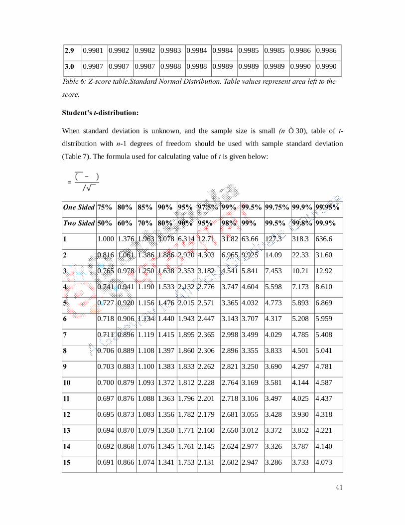
41

2.9 0.9981 0.9982 0.9982 0.9983 0.9984 0.9984 0.9985 0.9985 0.9986 0.9986

3.0 0.9987 0.9987 0.9987 0.9988 0.9988 0.9989 0.9989 0.9989 0.9990 0.9990

Table 6: Z-score table.Standard Normal Distribution. Table values represent area left to the

score.

Student's t-distribution:

When standard deviation is unknown, and the sample size is small (n ≤ 30), table of t-

distribution with n-1 degrees of freedom should be used with sample standard deviation

(Table 7). The formula used for calculating value of t is given below:

�=(� − �)

� √�⁄

One Sided 75% 80% 85% 90% 95% 97.5% 99% 99.5% 99.75% 99.9% 99.95%

Two Sided 50% 60% 70% 80% 90% 95% 98% 99% 99.5% 99.8% 99.9%

1 1.000 1.376 1.963 3.078 6.314 12.71 31.82 63.66 127.3 318.3 636.6

2 0.816 1.061 1.386 1.886 2.920 4.303 6.965 9.925 14.09 22.33 31.60

3 0.765 0.978 1.250 1.638 2.353 3.182 4.541 5.841 7.453 10.21 12.92

4 0.741 0.941 1.190 1.533 2.132 2.776 3.747 4.604 5.598 7.173 8.610

5 0.727 0.920 1.156 1.476 2.015 2.571 3.365 4.032 4.773 5.893 6.869

6 0.718 0.906 1.134 1.440 1.943 2.447 3.143 3.707 4.317 5.208 5.959

7 0.711 0.896 1.119 1.415 1.895 2.365 2.998 3.499 4.029 4.785 5.408

8 0.706 0.889 1.108 1.397 1.860 2.306 2.896 3.355 3.833 4.501 5.041

9 0.703 0.883 1.100 1.383 1.833 2.262 2.821 3.250 3.690 4.297 4.781

10 0.700 0.879 1.093 1.372 1.812 2.228 2.764 3.169 3.581 4.144 4.587

11 0.697 0.876 1.088 1.363 1.796 2.201 2.718 3.106 3.497 4.025 4.437

12 0.695 0.873 1.083 1.356 1.782 2.179 2.681 3.055 3.428 3.930 4.318

13 0.694 0.870 1.079 1.350 1.771 2.160 2.650 3.012 3.372 3.852 4.221

14 0.692 0.868 1.076 1.345 1.761 2.145 2.624 2.977 3.326 3.787 4.140

15 0.691 0.866 1.074 1.341 1.753 2.131 2.602 2.947 3.286 3.733 4.073

42

16 0.690 0.865 1.071 1.337 1.746 2.120 2.583 2.921 3.252 3.686 4.015

17 0.689 0.863 1.069 1.333 1.740 2.110 2.567 2.898 3.222 3.646 3.965

18 0.688 0.862 1.067 1.330 1.734 2.101 2.552 2.878 3.197 3.610 3.922

19 0.688 0.861 1.066 1.328 1.729 2.093 2.539 2.861 3.174 3.579 3.883

20 0.687 0.860 1.064 1.325 1.725 2.086 2.528 2.845 3.153 3.552 3.850

21 0.686 0.859 1.063 1.323 1.721 2.080 2.518 2.831 3.135 3.527 3.819

22 0.686 0.858 1.061 1.321 1.717 2.074 2.508 2.819 3.119 3.505 3.792

23 0.685 0.858 1.060 1.319 1.714 2.069 2.500 2.807 3.104 3.485 3.767

24 0.685 0.857 1.059 1.318 1.711 2.064 2.492 2.797 3.091 3.467 3.745

25 0.684 0.856 1.058 1.316 1.708 2.060 2.485 2.787 3.078 3.450 3.725

26 0.684 0.856 1.058 1.315 1.706 2.056 2.479 2.779 3.067 3.435 3.707

27 0.684 0.855 1.057 1.314 1.703 2.052 2.473 2.771 3.057 3.421 3.690

28 0.683 0.855 1.056 1.313 1.701 2.048 2.467 2.763 3.047 3.408 3.674

29 0.683 0.854 1.055 1.311 1.699 2.045 2.462 2.756 3.038 3.396 3.659

30 0.683 0.854 1.055 1.310 1.697 2.042 2.457 2.750 3.030 3.385 3.646

40 0.681 0.851 1.050 1.303 1.684 2.021 2.423 2.704 2.971 3.307 3.551

50 0.679 0.849 1.047 1.299 1.676 2.009 2.403 2.678 2.937 3.261 3.496

60 0.679 0.848 1.045 1.296 1.671 2.000 2.390 2.660 2.915 3.232 3.460

80 0.678 0.846 1.043 1.292 1.664 1.990 2.374 2.639 2.887 3.195 3.416

100 0.677 0.845 1.042 1.290 1.660 1.984 2.364 2.626 2.871 3.174 3.390

120 0.677 0.845 1.041 1.289 1.658 1.980 2.358 2.617 2.860 3.160 3.373

∞ 0.674 0.842 1.036 1.282 1.645 1.960 2.326 2.576 2.807 3.090 3.291

Table 7: Student’s t-distribution table: The first column from the left indicates the degrees of

freedom (n-1). Depending on the degrees of freedom exhibited from the sample and the

confidence interval (one-sided/ two-sided), the critical value can be determined.

Estimating Population Means

In inferential statistics, the data is gathered from a random sample taken from the population

43

under study, and this data is used for drawing conclusions about the population. The

inferences are made based on estimates, and outcomes of hypothesis testing and predictions

are made for future observations. However, we know that sample mean is a point estimate

and is not exactly same to the population mean, but is indeed a representation of the

population. Also, the sampling distribution for the sample mean enables us to deduce the

uncertainty about the population mean.

Till now, we have discussed measures of central tendency (mean, mode, median, harmonic

mean, geometric mean) and for dispersion (range, variance, mean absolute deviation,

standard deviation). These parameters for a finite population are almost identical to their

sample analogues and can be used as point estimates of the population parameters. Point

estimation is the process of estimating a parameter based on a probability distribution,

calculated using observed data from the distribution, which can be regarded as the best

estimate of an unknown population parameter. They can be obvious at times, for instance,

when we use the sample mean to estimate population mean, but sometimes when there are

two or more possible estimates, the task is to choose the most appropriate one. For this

purpose, point estimates are compared based on their properties. The most important property

of all is consistency, which insists that with the increase in sample size, the estimate should

approximate closer to the population parameter. So the sampling distribution of the sample

mean is centred at the population mean and the distribution further approaches the normal

distribution the sample size increases, and the variance tends to decrease, simultaneously. So

other point estimates derived from sample parameters as sample variance, sample standard

deviation, etc.,and also provide consistent estimates for their respective population

parameters.

Unbiasedness is another property of point estimates. Principle of unbiased estimation states,

“When choosing among several different estimators, select one that is unbiased”.

Bias Properties of Some Common Estimates (3)

E(X) = µ—the sample mean is an unbiased estimator of the population mean.

E (S2) = σ2—the sample variance is an unbiased estimator of the population variance.

E(S) ≠σ-The sample standard deviation is a biased estimator of the population standard

deviation.

Other criteria to select best point estimator includes minimum variance and mean square error

(MSE). Therefore, if we have several estimates that are unbiased we choose the one with the

44

smallest variance for its sampling distribution. However, sometimes biased estimates with a

small bias and small variance are preferred over an unbiased estimate with a large variance.

In such a case to compare biased and unbiased estimates, mean square error is used for

accuracy of the estimate. Mean square is calculated using the following formula,

MSE= β2 + σ2, where β is the estimator bias and σ2 is the variance. So for an unbiased

estimator, β2 will be zero and MSE = σ2.

Sometimes, as mentioned above a biased estimator is preferred over an unbiased estimator

and the decision is made based on the above formula. For example, A and B are two estimates

of population parameters, where A is an unbiased estimator and B is a biased estimator. We

have, for A: Variance, σ2 = 50 and bias, β = 0;

and for B: Variance, σ2 = 20 and bias, β = 3. We calculate MSE for both A and B,

MSEA = σ2 = 50, and

MSEB = β2 + σ2 = 9 + 20 = 29.

In this case MSEA> MSEB, and we shall use the estimate with lower mean square error, so

here we shall choose B as the better point estimate than B, despite the fact that it is a biased

estimate.

Thus, we see that it is a combination of biasedness, variance and mean square error, which

help us to decide on the best point estimate for a given population parameter.

Confidence interval:

Point estimates fail to express the uncertainty of the estimate, but provide us with one reliable

value to be used for a population parameter. It is desirable to have a range in such a case,

which convinces to include most of the values of a population parameter. Counter to point

estimate is the interval estimate, which provides us the range in which the given parameter is

expected to lie if the same experiment is repeated a number of times. Confidence interval

indicates the probability of finding a true population parameter in the given prescribed range.

So this provides us with a range extending on both sides of the sample parameter, where the

probability of finding the true population parameter is maximum. Thus, confidence interval is

formed of two-sided confidence limits and the individual one-sided counterparts are termed

as the lower and upper confidence bounds on two sides respectively.

When independent random samples are taken from a population, and a confidence interval is

calculated for each sample, then a certain percentage will tend to include an unknown

45

population parameter and this percentage is the confidence level. The most commonly used

confidence level is 95%, however, depending on the requirements, 90%, 99% and 99.9%, etc.

confidence intervals can also be obtained. The width of the confidence interval indicates the

uncertainty of finding the population parameter in a given range.

A confidence level is the probability value 1- α (often expressed as the equivalent percentage

value), and is the proportion (when the experiment is repeated a number of times) when the

confidence interval contained the population parameter. It is given as percentage, say for α

=5%, then confidence level = 1 - 0.05 = 0.95 or 95%. In other words, this indicates that we

are 95% confident or95% of the times when this experiment is repeated the unknown

population parameter will tend to fall in this interval. This precision can be increased by

increasing the percentage of confidence level, i.e. by decreasing the value of α. Confidence

level is also called as degree of confidence or the confidence coefficient.

For observation with normal distribution, whose variance is σ2 , sample mean is X and when

the sampling distribution has mean equal to the population mean μ , then variance of the

sample distribution is σ2/n, where is n is the number of samples. In this case

( ) ( )n/σ/μXZ −= also has a normal distribution.

For a given sample, there is a small probability (α) that the sample parameter would fall in

one of the tail regions (shown in Figure 10). There are two tails, one on each side and the area

enclosed in each of them is given by α/2. Thus, we can say that there is a total probability of

α that a sample proportion will not fall in the given confidence interval, i.e. in either of the

two tail regions. Alternatively, there is a probability of 1-α that the sample proportion will fall

under the confidence interval (inner region). The Z-scores given to the boundaries lining the

inner region are represented as -Zα/2 and Zα/2, and arereferred as the critical value.

46

Figure 10: Confidence interval in a normal distribution curve is shown here. The

regions in the tail region of the curve are excluded from the confidence interval.

In the figure, with confidence interval 95% (the lined region, four central blocks),

each tail region contains 2.5% (on each side). The central region accounts for the

confidence region and as is evident from the figure, most of the values are

destined to fall under the inner region (95% of the values in this case). For 99%

confidence, the shaded region marked as 2% on both sides are also included.

Some common values of α and Z are given in table below. Normal distribution is symmetric

and, therefore the area below -Zα/2 is same as the area above Zα/2 (Figure 10).

α/2 0.500 0.100 0.050 0.025 0.010 0.005

Z 0.000 1.282 1.645 1.960 2.326 2.576

Significance level is the probability of obtaining a value in the critical region, even when the

null hypothesis is correct, indicating the probability of making a Type I error. It is denoted as

α, significance value. It is often set at 0.01 or 0.05, which indicates, 1% or 5% error

respectively .i.e. in a test with 0.05 set as the α value, it is acceptable to be wrong five times

out of the 100 times the experiment is conducted.

47

The range and the confidence interval for a mean can be calculated as follow:

so the confidence interval can be given as

( ) ( )

−

n1.96σX,

n1.96σX +

Here we have determined 95% confidence interval for a sample value of X, σ and μ and

sample size n. However, 95% is used here, but in principle, we can opt for higher confidence

level as 99% or 99.9%. So if we want to obtain a confidence level of 99%, then looking at the

table above, we know

( ) ( ) 0.99n

2.576σXμn

2.576σXP =+

≤≤− , and the interval can be given as

( ) ( )

−n

2.576σX,n

2.576σX +

The two equations obtained for 95% and 99%, indicates that for the same mean, standard

deviation and same sample size, with the increase in the confidence interval, the length of

interval increases along with the chance that the interval generated would contain the

population parameter, μ.

This calculation using Z-score can be used if the standard deviation, σ of the population is

known. However, if the population standard deviation is unknown and we want to estimate

the mean, in such a case t-distribution has to be used, instead of the normal distribution. Here,

we need to calculate sample standard deviation S and construct tscore

( ) ( )n/S/μX − , here this has Student's t-distribution with n-1 degrees of freedom and doesn't

depend on μand σ.

( ) ( )( )

( ) ( )( ) ( )( )

( ) ( ) ( )

( ) ( ) 0.95n

1.96σXμn

1.96σXP

get, further wewith

0.95n

1.96σμXn

1.96σP

0.951.96n/σ/μX1.96P

get wefor Z,n/σ/μXngSubstituti

ondistributi normal standardon based0.951.96Z1.96Pn/σ/μXZ

=+

=

=

==

≤≤−

≤−≤

−

≤−≤−

−

≤≤−−

48

The procedure used for calculating the 95% confidence interval for a population mean,

when the population variance is unknown uses the critical values from Student's t-

distribution table. The equivalent formula used in this case is

( ) ( )[ ]0.95n/SCXμn/SCXP =+≤≤− , so the interval can be given as

( ) ( )[ ]n/SCX,n/SCX +− .

Suppose the sample size is 20, i.e., n = 20, therefore, degrees of freedom, n-1 = 19. For

a confidence interval of 95%, using the student's t-distribution table the value of C =

2.093. So the interval in this case is ( ) ( )[ ]n/S2.093X,n/S2.093X +− .

Test of hypothesis:

A test of hypothesis is performed to validate the outcome of an experiment; it is called

statistically significant if it unlikely to have occurred by chance alone, as per the

predetermined threshold probability, i.e. the significance level. The phrase “test of

significance” was coined by Ronald Fischer (8). It is used to infer the probability that a set

hypothesis is true or not.

We start with defining the null hypothesis and alternate hypothesis. The null Hypothesis is the

claim of “no difference” and is denoted as H0. This is usually the default position. Situations

like no difference between means of two data sets, no relationship between two variables, no

effect of treatment on the experimental subjects, etc., are supposed for the null hypothesis.

Rejecting the null hypothesis, will give us the counter hypothesis, called the alternate

hypothesis, which indicate “a difference in the population”, and is the outcome a researcher

would usually look for. An alternate hypothesis is indicated as H1. This includes situations

like difference between the means of two data sets, establishing a relationship between two

variables or measurable effect of a given treatment on experimental subjects.

The steps involved in Hypothesis testing can be listed as follow:

1. Formulate the null hypothesis and the alternate hypothesis to suit the experiment.

2. Select a test statistic that can be used to analyse the truth of the null hypothesis. There are

different types of test statistic, which are used depending on the sampling distribution of the

data set, and critical values are defined for rejecting the null hypothesis. (In the previous

section, Z and t statistic are already mentioned, they can also be used.) The critical values are

the cut-offs that decide the region, called the critical region or the rejection region, for which

49

the null hypothesis would be rejected.

3. Determine the P-value. P-value is the probability of obtaining a test statistic at least as

extreme as the one that was actually observed, assuming that the null hypothesis is true(9).

Smaller P-values provide evidence against the null hypothesis.

4. Compare the obtained p-value to an acceptable significance value (α). If p ≤ α, we

conclude that the observed effect is statistically significant, and the null hypothesis is rejected

and the alternate hypothesis is termed valid. Significant value indicates that the observed

difference is not likely due to chance (significance level explained below).

When sample data is used to make inference about the population parameter, statistical

uncertainty persists and therefore, proving or disproving either of the hypotheses (null and

alternate) cannot be validated. In such a situation, the decision is made based on probability

and another probability of making a false decision is accepted. Two types of errors are

defined for this: Type I and Type II errors.

Type I error is defined as the probability of falsely rejecting the null hypothesis, i.e. a null

hypothesis is true, and we incorrectly reject it. Type II error is defined as the probability of

not rejecting the null hypothesis, when the null hypothesis is actually false, i.e. the true

parameter value which is specified by the alternate hypothesis is conformed to the null

hypothesis.

In statistical significance testing, we have two alternative ways to proceed with the test

statistic, one-tailed and two-tailed test. It depends on the likelihood of the presence of

extreme values in the data set on either direction i.e. one of the extreme sides or both the

sides. The terminology of 'tail' is used because the frequency at the extremes is usually

smallsmall and in a bell curve, it looks like extending tails. They are also termed as one-sided

or two-sided. Further, if the test statistic is always positive (or zero), one-tailed test is

preferred, and the two-tailed tests are used when both positive and negative values are

possible.

Test of a mean: population variance known:

When there is a single sample and the population variance is known, then we will use Z-

statistic. The steps involved in a two-tailed hypothesis test are listed below:

50

In this case the null hypothesis H0: μ = μ0, i.e. the two means are equal. The alternate

hypothesis H1: μ ≠ μ0, i.e. the two means are not equal.

Choose an appropriate significance level α = 0.05 or 0.01.

Determine the critical region, that is, the region of values of Z in the upper and lower α/2

tails of the sampling distribution for Z when μ = μ0.

Compute the Z-statistic: Z = (���)� √�⁄ for a given sample and sample size n, σ is the population

standard deviation, X is the sample mean.

Reject the null hypothesis if the test statistic Z computed in step 4 falls in the critical region

for this test; otherwise, do not reject the null hypothesis.

Test of a mean: population variance unknown

When there is a single sample and the population variance is unknown, then we will estimate

population variance by using a sample variance, s2 and apply t-statistic. The steps involved in

a two-tailed hypothesis test are listed below (3):

In this case the null hypothesis, i.e. the two means are equal. The alternate hypothesis H1: μ ≠

μ0, i.e. the two means are not equal.

Choose an appropriate significance level α = 0.05 or 0.01.

Determine the critical region for the appropriate t- distribution, that is the region of values of

tin the upper and lower α/2 tails of the sampling distribution for Student's t- distribution with

n-1 degrees of freedom (where n is the sample size) when μ = μ0.

Compute the t-statistic: t = (���)� √�⁄ for a given sample and sample size n, s is the sample

standard deviation and X is the sample mean.

Reject the null hypothesis if the test statistic tcomputed in step 4 falls in the critical region for

this test otherwisedoes not reject the null hypothesis.

Chi-squared test: Goodness-of-fit test

A goodness-of-fit test is used to test the hypothesis that the observed frequency distribution

fits (or conforms to) some expected distribution. It is used to see if the variation in the data

obtained/ observed is just due to chance or is it due to one of the variables under-involved.

51

Goodness-of-fit hypothesis tests are always right-tailed. It is appropriate for nominal or

ordinal measurements.

Null hypothesis: H0: There is no significant difference between the observed and the expected

frequencies.

Alternate hypothesis: H1: There is a significant difference between the observed and expected

frequencies.

For any given event, there is an expected set of values and the frequency of these values can

be given as expected Frequencies.

If all expected frequencies are equal, then expected frequency can be given as

� = � �⁄ , where n represents the number of trials and k represents the number of different

categories.

Therefore, an expected frequency is the sum of all observed frequencies divided by the

number of categories.

If all expected frequencies are not all equal, each expected frequency is calculated by taking

the product of the sum of all observed frequencies (n) and the probability (p) for a particular

category. It is given by the formula: � = ��

Goodness-of-fit Test for Multinomial Experiments

Multinomial Experiment: An experiment is said to be multinomial, when the number of trials

is fixed, and these trials are independent. The probabilities for the different categories remain

constant for each trial, and the outcome of each trial must be put under exactly one of these

categories.

52

Figure 11: With the significance level set at 0.01, the critical value is determined.

If the χ2 exceeds the critical value, it falls on the right side of the critical point

and the null hypothesis is rejected.

Test Statistic used for multinomial experiments(χ2) is given as:

�� � � ������

�, where O is the observed frequency for each category, E is the expected value

for a given category. The difference between O and E is calculated for each category and is

divided by the expected frequency of a particular category. The values thus obtained are

added and is indicated as the value of χ2.

The degree of freedom (df) is calculated: df = k-1

Level of significance has to be fixed to look upto a table and is usually fixed as p < 0.05.

This value of χ2 is then compared with the critical value from the table (Table 8),

corresponding to the degrees of freedom (df = k-1) for the experiment. If the critical value

exceeds the χ2 value obtained from the formula, the null hypothesis is accepted, else the null

hypothesis is rejected (Figure 11). A close agreement between expected and observed values

leads to a small value of χ2. On the other hand, a large difference betweenexpected and

observed values will lead to a large value of χ2.

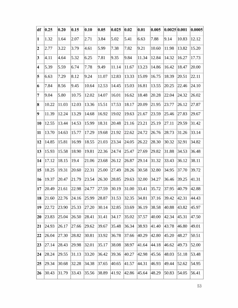
53

df 0.25 0.20 0.15 0.10 0.05 0.025 0.02 0.01 0.005 0.0025 0.001 0.0005

1 1.32 1.64 2.07 2.71 3.84 5.02 5.41 6.63 7.88 9.14 10.83 12.12

2 2.77 3.22 3.79 4.61 5.99 7.38 7.82 9.21 10.60 11.98 13.82 15.20

3 4.11 4.64 5.32 6.25 7.81 9.35 9.84 11.34 12.84 14.32 16.27 17.73

4 5.39 5.59 6.74 7.78 9.49 11.14 11.67 13.23 14.86 16.42 18.47 20.00

5 6.63 7.29 8.12 9.24 11.07 12.83 13.33 15.09 16.75 18.39 20.51 22.11

6 7.84 8.56 9.45 10.64 12.53 14.45 15.03 16.81 13.55 20.25 22.46 24.10

7 9.04 5.80 10.75 12.02 14.07 16.01 16.62 18.48 20.28 22.04 24.32 26.02

8 10.22 11.03 12.03 13.36 15.51 17.53 18.17 20.09 21.95 23.77 26.12 27.87

9 11.39 12.24 13.29 14.68 16.92 19.02 19.63 21.67 23.59 25.46 27.83 29.67

10 12.55 13.44 14.53 15.99 18.31 20.48 21.16 23.21 25.19 27.11 29.59 31.42

11 13.70 14.63 15.77 17.29 19.68 21.92 22.62 24.72 26.76 28.73 31.26 33.14

12 14.85 15.81 16.99 18.55 21.03 23.34 24.05 26.22 28.30 30.32 32.91 34.82

13 15.93 15.58 18.90 19.81 22.36 24.74 25.47 27.69 29.82 31.88 34.53 36.48

14 17.12 18.15 19.4 21.06 23.68 26.12 26.87 29.14 31.32 33.43 36.12 38.11

15 18.25 19.31 20.60 22.31 25.00 27.49 28.26 30.58 32.80 34.95 37.70 39.72

16 19.37 20.47 21.79 23.54 26.30 28.85 29.63 32.00 34.27 36.46 39.25 41.31

17 20.49 21.61 22.98 24.77 27.59 30.19 31.00 33.41 35.72 37.95 40.79 42.88

18 21.60 22.76 24.16 25.99 28.87 31.53 32.35 34.81 37.16 39.42 42.31 44.43

19 22.72 23.90 25.33 27.20 30.14 32.85 33.69 36.19 38.58 40.88 43.82 45.97

20 23.83 25.04 26.50 28.41 31.41 34.17 35.02 37.57 40.00 42.34 45.31 47.50

21 24.93 26.17 27.66 29.62 39.67 35.48 36.34 38.93 41.40 43.78 46.80 49.01

22 26.04 27.30 28.82 30.81 33.92 36.78 37.66 40.29 42.80 45.20 48.27 50.51

23 27.14 28.43 29.98 32.01 35.17 38.08 38.97 41.64 44.18 46.62 49.73 52.00

24 28.24 29.55 31.13 33.20 36.42 39.36 40.27 42.98 45.56 48.03 51.18 53.48

25 29.34 30.68 32.28 34.38 37.65 40.65 41.57 44.31 46.93 49.44 52.62 54.95

26 30.43 31.79 33.43 35.56 38.89 41.92 42.86 45.64 48.29 50.83 54.05 56.41

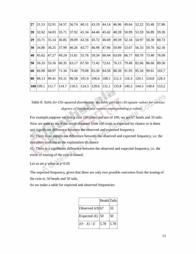
54

27 31.53 32.91 34.57 36.74 40.11 43.19 44.14 46.96 49.64 52.22 55.48 57.86

28 32.62 34.03 35.71 37.92 41.34 44.46 45.42 48.28 50.99 53.59 56.89 59.30

29 33.71 35.14 36.85 39.09 42.56 45.72 46.69 49.59 52.34 54.97 58.30 60.73

30 34.80 36.25 37.99 40.26 43.77 46.98 47.96 50.89 53.67 56.33 59.70 62.16

40 45.62 47.27 49.24 51.81 55.76 59.34 60.44 63.69 66.77 69.70 73.40 76.09

50 56.33 53.16 60.35 63.17 67.50 71.42 72.61 76.15 79.49 82.66 86.66 89.56

60 66.98 68.97 71.34 74.40 79.08 83.30 84.58 88.38 91.95 95.34 99.61 102.7

80 88.13 90.41 93.11 96.58 101.9 106.6 108.1 112.3 116.3 120.1 124.8 128.3

100 109.1 111.7 114.7 118.5 124.3 129.6 131.1 135.8 140.2 144.3 149.4 153.2

Table 8: Table for Chi-squared distribution: the table provides chi-square values for various

degrees of freedom and various corresponding p-values.

For example,suppose we toss a coin 100 times and out of 100, we get 67 heads and 33 tails.

Now we want to see if the result obtained from 100 trials is expected by chance or is there

any significant difference between the observed and expected frequency.

H0: There is no significant difference between the observed and expected frequency, i.e. the

outcomes conform to the explanation of chance

H1: There is a significant difference between the observed and expected frequency, i.e. the

event of tossing of the coin is biased.

Let us set p value at p<0.05

The expected frequency, given that there are only two possible outcomes from the tossing of

the coin is: 50 heads and 50 tails.

So we make a table for expected and observed frequencies

Heads Tails

Observed (O) 67 33

Expected (E) 50 50

(O – E) / E 5.78 5.78

55

�� = � (���)�

� =5.78 + 5.78 = 11.56

Degrees of freedom = k – 1 = 2 - 1 =1

Now we look at the table for a critical value (Table 8), given that degrees of freedom (df) is 1

and p value is 0.05, so the critical value is 3.84.

The value of χ2 we obtained is 11.56 which is greater than the critical value and hence falls in

the tail region and hence we reject the null hypothesis. We conclude that there is a significant

difference between the observed and expected frequency, i.e. the event of tossing of the coin

is biased at a given level of significance.

Testing independence between two variables: Contingency Table (or two-way frequency

table):

A contingency table is used to determine whether there is a statistically significant relation

between two variables, the frequencies of two variables are presented in columns and rows of

a contingency table, also known as cross-tabulation table. One variable occupies the rows and

the other fits in the columns; hence the table must have atleast two rows and two columns.

Tests of Independence are always right-tailed.

Null hypothesis: H0: The row variable is independent of the column variable, i.e. the row and

column variable of the given contingency table are not related.

Alternate Hypothesis: H1: The row variable is dependent (related to) the column variable, i.e.

the row and column variables of the given contingency table are related.

Test of Independence Test Statistic:�� = � (���)�

�

Degrees of freedom: (r-1)*(c-1), where r and c are the numbers of rows and columns

respectively.

E = row total* column total/ grand total

Grand total = total number of all observed frequencies in the table.

Level of significance has to be fixed to look upto a table and is usually fixed as p < 0.05

(95% confidence).

This value of χ2 is then compared with the critical value from the Table 8, corresponding to

the degrees of freedom (df) for the experiment. If the critical value exceeds the χ2 value

56

obtained from the formula, the null hypothesis is accepted; else the null hypothesis is

rejected.

ANOVA: Analysis of Variance

It is a method for testing the hypothesis that means of three or more populations are equal. So

the hypothesis can be put as

H0: μ1= μ2 =μ3 = … μk

H1: At least one of the mean is different.

This can be considered as an extension of Z test or t-test, which was used to compare two

populations; here ANOVA facilitates the comparison of more than two groups. ANOVA can

be further specialised as one-way ANOVA (where the groups differ each other based on a

single factor), two-way, three-way, and N-way ANOVA, depending on the number of

variables. For instance in two-way ANOVA the effects of two variables on the groups under

study is examined. These are widely used to study randomised block design. In such a design,

there is one factor (such as drug treatment), whose effect is being examined on the blocks.

Here the blocks are subsets of a population categorized based on another factor, such as age,

locality, community, etc., which may significantly contribute in error variance if left

unconsidered. In such a condition, both the factor effect and the block effect are called the

main effects. Also,the interaction between the factor and block can be studied where a

particular combination may exhibit interesting characteristics.

The main purpose of ANOVA is to compare more than two populations and can be

considered as a generalization of t-test for three or more groups. However, the difference lies

in the fact that one-sided t-test, after the rejection of the null hypothesis, the alternative

indicated which of the two means is greater, whereas the corresponding test, F-test, in

ANOVA tells you that the means are different but no information about the differences in

mean can't be obtained. In order to get that information, special additional tests have to be

performed.

The test statistic is the ratio of estimates of two sources of variation called the within- group

variance and the between-group variance. Now, when studying the effect of a given treatment

to more than two groups and if the treatment is making any difference among the groups,

then it is expected that the between group variance would be higher than the within group

variance. These variances divided by their degrees of freedom are called mean squares, where

57

degrees of freedom is denoted as nw and nb for within group and between group variances,

respectively. As mentioned earlier, the ratio of these mean squares is the test statistic for

ANOVA. Now, when the means of these groups are equal, this ratio has an F distribution with

nb in the numerator and nw in the denominator and this F distribution is used to determine

whether or not to reject the null hypothesis. However, this F distribution is more complex

than t-distribution as it involves two degrees of freedom parameters.

The response variable is the variable you are comparing. The factor variable is a categorical

variable being used to define the groups.

We shall discuss the procedure using an example. We shall continue with one-way ANOVA,

one-way because each value is classified in exactly one way.

Suppose we have scores of fifteen students in geography, where students have been divided

into three sets,

1st set: R, Routine, who have not attended extra classes and did not have internet access at

home.

2nd set: C, those who have taken extra Classes, does not have internet access at home.

3rd set: I, those with access to Internet at home, who have not attended extra classes.

The null hypothesis is that all the means for the three sets are equal;

H0: μ1= μ2 =μ3

The alternative hypothesis is that at least one of the mean is different.

Data set:

Routine Classes Internet

3 10 10

5 7 12

6 8 15

2 6 14

4 9 9

We wish to know the impact of each of these conditions on these students in three sets.

Analysis of variance allows us to compare different samples at different point of time or

58

conditions. The main steps involved in Analysis of Variance are mentioned below:

Step 1: Calculate variance, i.e. sum of squares, for each set of samples. This is called as sum

of squares within groups.

Step 2: Calculate variance between groups, called as sum of squares between groups.

Step 3: Take the whole sample, consider as one complete study, and calculate variance from

the mean of all the samples taken together, known as the total sum of squares.

Step 4: Calculate degrees of freedom and combine them with the sum of squares.

Step 5: Calculate F-ratio, and look at the critical value table. If it falls in the rejection area,

reject the null hypothesis. Else, we fail to reject the null hypothesis.

Now we shall start with the actual data set and we will go through each step calculation in

detail:

Total sum of squares = Sum of squares between groups + Sum of squares within groups

Calculating Sum of Squares within Groups:

Step 1: Calculate mean of the each data set.

Step 2: Calculate deviation of each observation from the mean using formula: x-μ

Step 3: Calculate square of the deviation, variance using formula: (x-μ) 2

Step 4: Calculate the sum of variance, denoted as SSW, sum of squares within groups.

Routine x-μ (x-μ)2 Classes x-μ (x-μ)2 Internet x-μ (x-μ)2

3 -1 1 10 2 4 10 -2 4

5 1 1 7 -1 1 12 0 0

6 2 4 8 0 0 15 3 9

2 -2 4 6 -2 4 14 2 4

4 0 0 9 1 1 9 -3 9

μ=4 sum=10 μ=8 sum=10 μ=12 sum=26

Sum of Squares within Groups, SSW = 10 + 10 + 26 = 46

59

Calculating Total Sum of Squares:

Step 1: Calculate mean of all the observations from the three data sets taken together. This is

called as the grand mean.

3+10+10+5+7+12+6+8+15+2+6+14+4+9+9 = 120/15 = 8

Step 2: Calculate deviation of each observation from the mean using formula: x-μ

Step 3: Calculate square of the deviation, variance using formula: (x-μ)2

Step 4: Calculate the sum of variance, denoted as TSS, total sum of squares.

Sum of variance is found to be 206.

Total sum of Squares, TSS = 206

Calculating Sum of Squares between Groups:

Step1: Since we already have the combined mean of all the samples taken together, i.e. 8 and

also mean of individual data sets, 4, 8 and 12 respectively, we calculate individual mean –

total mean for each data set.

Data set 1: 4 – 8 = -4; Data set 2: 8 – 8 = 0 and Data set 3: 12 – 8 = 4

Step 2: Calculate square of each of the deviation calculated in Step 1. This is the variation

between each sample mean and the grand mean.

Data set 1: 16; Data set 2: 0 and Data set 3: 16

Step 3: Calculate the sum of these squares obtained

Sum of squares: 16 + 0 +16 = 32

Step 4: Multiply the sum of squares with n, the sample size of individual data set.

32 * 5 = 160, this is the sum of squares between groups.

Sum of squares between groups, SSB = 160

So now we have all the values of the equation:

Total sum of squares = Sum of squares between groups + Sum of squares within groups

206 = 160 + 46

So we see that calculating any two of the three expressions of the above equation can serve

the purpose as the third can be derived from the other two values.

Calculating degrees of freedom:

A degree of freedom is a measure for the number of ways each value can vary before the rest

60

of the values are predetermined. It is often one less than the number of values.

Degrees of freedom between groups = number of groups – 1= 3 – 1 = 2

Degrees of freedom within groups = Total number of observations – number of groups = 15 –

3 = 12

Calculating F value through mean squares:

Step 1: ( ) 802

160reedomdegreesoff

roupsesBetweenGSumofSquarBMS ===

Step 2: ( ) 3.8331246

reedomdegreesoffoupsesWithinGrSumofSquarWMS ===

Step 3: Ratio of above two expressions = MS (B)/MS (W) = 80/ 3.833 = 20.87

F = 20.87; However, the notation used for F, includes the degrees of freedom between groups

(nb) and within groups (nw) and is written as F (nb, nw). In our example,

Degree of freedom from numerator, nb = 2

Degrees of freedom from denominator, nw = 12

F (2, 12) = 20.87

for p < 0.05, critical value is 3.89, looked from table and F = 20.87,

therefore, 20.87 falls in the right of critical value and thus fall in the rejection area and hence

in this example, we reject the null hypothesis.

Here, the null hypothesis is that the means of the three sets of students were the same,

however we reject the null hypothesis and hence conclude that atleast one of the three sets

has a different mean. ANOVA doesn't tell us as to which set is different.

The F-test is the right tail statistic.

Correlation and Regression: It is necessary often to establish a relationship between two variables. Correlational

techniques are used to examine the relationship of the two variables. Two basic correlational

techniques are (5):

Correlation: It is used to establish and quantify the strength and direction of the relationship

between two variables.

Regression: It is used to express the functional relationship between two variables, so that

the value of one variable can be predicted from knowledge of the other.

61

Correlation: A correlation coefficient is used to determine linear association between two

variables and is denoted as r. The value of r ranges from -1 to +1, where +1 indicates a

perfect relationship in a positive linear sense and -1 indicates a perfect relationship in a

negative linear sense. When the correlation coefficient is zero, it indicates that there is no

linear relation between the two variables. When the value of r is beyond ±0.5, it is considered

as a strong relationship, and when coefficient is between zero and ±0.5, it isusually

considered as a weak relationship. Correlation is the study of interdependence of two

variables.

The Pearson correlation coefficient (ρ) is a population parameter which measures the

association between two variables. Bivariate normal distribution usually represents the

relationship between two associated variables, commonly plotted as a scatter diagram, where

one of the variable is plotted on x-axis and the other variable is plotted in y-axis, and each

point plotted on the graph shows the paired value of two variables, i.e. each individual (X,Y)

pair is plotted as a single point. It can be considered as a probability distribution for X and Y,

both of which have a normal distribution and thus form a density function for their paired

values. The sample correlation coefficient, as mentioned earlier is represented as r and is the

sample estimate of ρ, which can be obtained from paired values of two variables.

Using a scatter plot, linear correlationis easily visualised. Figure 12 shows the patterns

acquired by the data depending on their correlation strength and direction:

The formula for used for calculating Pearson sample product moment correlation coefficient

(simply known as linear correlation coefficient) is given as,

( )( )( ) ( ) ( ) ( )2222 ∑∑∑∑

∑∑∑−−

−

yynxxn

yxxyn=r ,

where n is the number of pairs of data observed

(x, y) indicates paired data

Σx is the sum of all x-values.

Σx2is the sum of the squares of each x value taken individually.

(Σx) 2 is the square of the sum of all x values.

Σxy is the sum of the products of x and y, which form a pair. Say if the pairs are (x1,y1),

(x2,y2)... (xn,yn), then Σxy is (x1y1) + (x2y2) +...+ (xnyn).

As mentioned earlier r is the sample estimate of ρ, which is a population parameter and is

alinear correlation coefficient for all paired data in the population.

62

Testing hypothesis about the correlation coefficient: Here our aim to determine if there is any

significant linear correlation between two variables of not. So we make the hypothesis

stating,

H0 :ρ = 0 (no significant linear correlation)

H1 : ρ ≠ 0 (significant linear correlation)

Figure 12: Scatter plots displaying patterns obtained for positive and negative

linear correlation. Last two plots show examples for no correlation and

63

nonlinearcorrelation.

The test is based on a t-test. The significance test for Pearson's correlation coefficient is given

bythe formula for t (tdf) and is dependent on the degrees of freedomdf, which is calculated as

df = n – 2, where n is the number of pairs.

( )21 2

−−

nr

r=tdf

By looking at the table, the critical value for the respective value of t and df is obtained. If the

absolute value of the test statistic exceeds the critical value obtained from the table, we reject

the null hypothesis H0, i.e. we conclude that there is significant linear correlation, else

ifabsolute value of the test statistic falls below the critical value obtained from the table, we

fail to reject the null hypothesis and conclude that there is no significant linear correlation as

per the data.

Regression:

When two variables are highly correlated, it is possible to predict the dependence

relationship. The value of one of the two variables, a dependent variable can be predicted

from the value of the other, independent variable using regression. Thus, the regression

equation expresses the relationship between X, the independent variable, and Y, the dependent

variable.

Linear Regressionis a statistical approach for modelling the relationship between a

scalar dependent variable (Y) and one or more independent/explanatory variables (X.) Simple

Linear Regression is a relationship between one dependent and one independent variable.

When there are two or more dependent variables(X1,X2…) which help in predicting(Y), such

a case is called Multiple Linear Regression.

Scatter graph allows us to observe the relationship between two variables. The graphs shown

in Figure 11 indicate a general pattern, and this can be summarized by drawing a line which

can explain the general behaviour pattern of the given data, which is called the line of best fit.

For this purpose we use equation for a line which is given as Y = mX + b, where b = the

intercept (point where the line crossed y-axis) and m = slope of the line.

64

Simple Linear Regression Analysis: In such analysis the equation used for line is given as Y

= β0 + β1X1, where β0 is the intercept and β1 is the slope of the line and X is the independent

variable. If β1> 0, then there is a positive relationship between X and Y and a negative value

of β1 indicates a negative relationship. If there is no relationship between X and Y, then β1 =

0.

While using practical data, all the points may or may not fall exactly on the line.The sum of

the squares of all the deviations from all the points from the line are minimized by drawing a

line through the data set using the principle of least squares. This line of best fit is obtained

through a scatter plot measurement and is also called as the regression line or least squares

line. Therefore, for use in practical purposes the general equation stated above is modified to

account for error between observed and predicted values of Y.

Thus, the simple linear regression model is given as

Y = β0 + β1X+ e,

Where e indicates the residual error. eis estimated by the deviation of the observed value Y

from the expected value Ŷ, which is calculated using the regression equation.

Further, the estimated regression equation for Y on X is given as Ŷ = b0 + b1X. So for a given

value of X, if we have an equation for best fit straight line, we can estimate the value for Y.

So for each observation e = Y- Ŷ , since this measures the vertical deviation of the actual

observation from the expected value, it can be positive if the observed value is above the

regression line or negative if the observation value lies below the regression line. These

deviations are squared to make all of them positive. A line which minimises this sum of

squared distances,and fits the data best, is called as the least squares line.

Σ (Yi- Ŷi)2 = Σe2

A least squares regression selects the line with the lowest total sum of squared prediction

errors, and this value is called the Sum of Squares of Error or SSE.The Sum of Squares

Regression (SSR) is the sum of the squared differences between the prediction for each

observation and the population mean.

The Total Sum of Squares (SST) is equal to SSR + SSE.

Mathematically,

65

SSR = ∑ (Ŷi – � ) (measure of explained variation)

SSE = ∑ (Yi – Ŷ i ) (measure of unexplained variation)

SST = SSR + SSE = ∑ (Yi – � ) (measure of total variation in y)

� =��

�

The proportion of total variation (SST) that is explained by the regression (SSR) is known as the Coefficient of Determination and is often referred to as R,

� =������ = ��

The value of R can range between 0 and 1, and the higher its value, the more accurate the regression model is. It is often referred to as a percentage.

Coefficient of Determination

0.81≤R≤1 à Strong Regression Relationship

0.49≤R<0.81 à Moderate Regression Relationship

0.25≤R<0.49 à Weak Regression Relationship

0.0≤R<0.25 à No Regression Relationship Multiple Regression Analysis: In such regression analysis the equation used for line is given

as Y = β0 + β1X1+ β2X2+….+ βnXn, where β0 is the intercept and β1, β2.. βn packed together

defines the slope of the line and Xn,the independent variable. If βn> 0, then there is a positive

relationship between Xn and Y and a negative value of βn indicates a negative relationship. If

there is no relationship between Xn and Y, then βn = 0.

The equation of line of best fit accounting error between observed and predicted values of Y,

is now given asY = β0 + β1X1+ β2X2+….+ βnXn + ϵ, where ϵis a random variable called error

term.

Further, the estimated regression equation for Y on X is given as Ŷ = b0 + b1X1+b2X2+….+bnXn.

So for a given value of X, if we have an equation for best fit straight line, we can estimate the

value for Y.

The value of R can range between 0 and 1, and the higher its value the more accurate the regression model is. It is often referred to as a percentage.

The Standard Error of a regression is a measure of its variability. It can be used in a similar manner as the standard deviation, allowing for prediction intervals.

66

y ± 2 standard errors will provide approximately 95% accuracy, and 3 standard errors will provide a 99% confidence interval.

Standard Error is calculated by taking the square root of the average prediction error.

Standard Error (s) =� �����(���)

, where n is the number of observations in the sample and k is

the total number of variables in the model

b is the per unit change in the dependent variable for each unit change in the independent variable. Mathematically:

� =∆y∆�

Testing for overall significance Testing hypothesis about the regression analysis depends uponCoefficient of Determination

R. Here our aim to determine if there is any significant linear regression between independent

and dependent variables or not. So we make the hypothesis stating,

H0 : ρ = 0 (no significant regression relationship exists)

H1 : ρ ≠ 0 (Significant regression relationship exists)

Test statistic F-test = MSR (Mean Square Regression)/MSE (Mean Square Error)

Now the MSE provides the estimate of σ2.

Standard Error (s) =√� �� = � �����(���)

Where n is the number of observations in the sample and k is the total number of variables in the model

MSR = ����

; where K is the number of independent variable.

If F-test = MSR/MSE, is more than critical value of F(α,k,(n-k+1)), H0is rejected. It means significant regression relationship exist. When F-test shows an overall significance, then the next step is to use t-test, to determine if each of the individual independent variables is significant. Further, a separate t-test is conducted for each of these to determine cause and effect relationship. Testing for Significance H0 : βi = 0 (Slope is not significantly different from 0)

H1 : βi≠ 0 (Slope is significantly different from 0)

67

Test Statistic t-test=bi/Sbi whereSbirepresents the standard error of bi.

��� =�

�Σ(��− �)�

Confidence Interval forβi:�� ± ��/� × ���

Wheretα/2 is the t value providing area of α/2 in the upper tail of thet-distribution with n-k degrees of freedom. If H0 is rejected, y intercept is significantly different from 0 and should be included in regression equation.