introduction to tatics ynamics - andy...

Introduction to

STATICSand

DYNAMICSAndy Ruina and Rudra Pratap

c Rudra Pratap and Andy Ruina, 1994-2008. All rights reserved. No part of this book may be reproduced, stored in aretrieval system, or transmitted, in any form or by any means, electronic, mechanical, photocopying, or otherwise, withoutprior written permission of the authors.

This book is a pre-release version of a book in progress for Oxford University Press.

Acknowledgements. The following are amongst those who have helped with this book as editors, artists, tex program-mers, advisors, critics or suggestors and creators of content: William Adams, Alexa Barnes, Joseph Burns, Jason Cortell,Gabor Domokos, Max Donelan, Thu Dong, Gail Fish, Mike Fox, John Gibson, Robert Ghrist, Saptarsi Haldar, Dave Heim-stra, Theresa Howley, Herbert Hui, Michael Marder, Elaina McCartney, Horst Nowacki, Kalpana Pratap, Richard Rand,Dane Quinn, C.V. Radakrishnan, Phoebus Rosakis, Les Schaeffer, Ishan Sharma, David Shipman, Jill Startzell, Saskya vanNouhuys, Tian Tang, Kim Turner and Bill Zobrist. We certify Arthur Ogawa, Ivan Dobrianov, and Stephen Hicks as TeXgeniuses. Mike Coleman worked extensively on the text, wrote many of the examples and homework problems and mademany figures. David Ho, R. Manjula and Abhay drew or improved most of the drawings. Credit for some of the homeworkproblems retrieved from Cornell archives is due to various Theoretical and Applied Mechanics faculty. Harry Soodak andMartin Tiersten provided some problems from their incomplete book. Our on-again off-again editor Peter Gordon has beensupportive throughout. Many other friends, colleagues, relatives, students, and anonymous reviewers have also made helpfulsuggestions.

Software we have used to prepare this book includes TEXshop (for LATEX), Adobe Illustrator, GraphicsConverter and MAT-LAB.

Brief ContentsFront tables . . . . . . . . . . . . . . . . . . . . . . . . . . . . . . . iBrief Contents . . . . . . . . . . . . . . . . . . . . . . . . . . . . . . 1Detailed Contents . . . . . . . . . . . . . . . . . . . . . . . . . . . . 2Preface . . . . . . . . . . . . . . . . . . . . . . . . . . . . . . . . . . 10

Part I: Basics for Mechanics 221 What is mechanics? . . . . . . . . . . . . . . . . . . . . . . . . . 222 Vectors . . . . . . . . . . . . . . . . . . . . . . . . . . . . . . . 363 FBDs . . . . . . . . . . . . . . . . . . . . . . . . . . . . . . . . 140

Part II: Statics 1784 Statics of one object . . . . . . . . . . . . . . . . . . . . . . . . . 1785 Trusses and frames . . . . . . . . . . . . . . . . . . . . . . . . . 2466 Transmissions and mechanisms . . . . . . . . . . . . . . . . . . . 3087 Hydrostatics . . . . . . . . . . . . . . . . . . . . . . . . . . . . . 3608 Tension, shear and bending moment . . . . . . . . . . . . . . . . 376

Part III: Dynamics 3969 Dynamics in 1D . . . . . . . . . . . . . . . . . . . . . . . . . . . 39610 Particles in space . . . . . . . . . . . . . . . . . . . . . . . . . . 51411 Many particles in space . . . . . . . . . . . . . . . . . . . . . . . 56212 Straight line motion . . . . . . . . . . . . . . . . . . . . . . . . . 58813 Circular motion . . . . . . . . . . . . . . . . . . . . . . . . . . . 62614 Planar motion of an object . . . . . . . . . . . . . . . . . . . . . 73415 Kinematics using time-varying basis vectors . . . . . . . . . . . . 82016 Constrained particles and rigid objects . . . . . . . . . . . . . . . 888

Appendices 956A Units & Center of mass theorems . . . . . . . . . . . . . . . . . . 956

Answers to some homework problems . . . . . . . . . . . . . . . . . 976Index . . . . . . . . . . . . . . . . . . . . . . . . . . . . . . . . . . 984Back tables . . . . . . . . . . . . . . . . . . . . . . . . . . . . . . . 989

1

Detailed ContentsFront tables i

Summary of mechanics . . . . . . . . . . . . . . . . . . . iSome basic definitions . . . . . . . . . . . . . . . . . . . . ii

Brief Contents 1

Detailed Contents 2

Preface 10General issues about content, level, organization and style, motivation,how to study and the use of computers.

0.1 To the student (please read) . . . . . . . . . . . . . . . . . . 140.2 A note on computation . . . . . . . . . . . . . . . . . . . . . 18

Box: Informal computer commands . . . . . . . . . . . . . 21

Part I: Basics for Mechanics 22

1 What is mechanics? 22Mechanics can predict forces and motions by using the three pillars of thesubject: I. models of physical behavior, II. geometry, and III. the basicmechanics balance laws. The laws of mechanics are informally summa-rized in this introductory chapter. The extreme accuracy of Newtonianmechanics is emphasized, despite relativity and quantum mechanics sup-posedly having ‘overthrown’ seventeenth century physics. Various usesof the word ‘model’ are described.

1.1 The three pillars . . . . . . . . . . . . . . . . . . . . . . . . 231.2 Mechanics is wrong, why study it? . . . . . . . . . . . . . . 291.3 The heirarchy of models . . . . . . . . . . . . . . . . . . . . 31

2 Vectors 36The key vectors for statics, namely relative position, force, and moment,are used to motivate needed vector skills. Notational clarity is empha-sized because correct calculation is impossible without distinguishingvectors from scalars. Vector addition is motivated by the need to addforces and relative positions, dot products are motivated as the tool whichreduces vector equations to scalar equations, and cross products are mo-tivated as the formula which correctly calculates the heuristically moti-vated quantities of moment and moment about an axis.

2

Chapter 0. Detailed Contents Detailed Contents 3

2.1 Notation and addition . . . . . . . . . . . . . . . . . . . . . 38Box 2.1 The scalars in mechanics . . . . . . . . . . . . . . 39Box 2.2 The Vectors in Mechanics . . . . . . . . . . . . . 40

2.2 The dot product of two vectors . . . . . . . . . . . . . . . . 56Box 2.3 ab cos � ) axbx C ayby C azbz . . . . . . . 61

2.3 Cross product and moment . . . . . . . . . . . . . . . . . . 65Box 2.4 Cross product as a matrix multiply . . . . . . . . . 75Box 2.5 The cross product is distributive over sums . . . . 76

2.4 Solving vector equations . . . . . . . . . . . . . . . . . . . . 85Box 2.6 Vector triangles and the laws of sines and cosines . 88Box 2.7 Existence, uniqueness, and geometry . . . . . . . 100

2.5 Equivalent force systems . . . . . . . . . . . . . . . . . . . . 105Box 2.8

Pmeans add . . . . . . . . . . . . . . . . . . . . 107

Box 2.9 Equivalent at one point ) equivalent at all points 108Box 2.10 A “wrench” can represent any force system . . . 109

2.6 Center of mass and gravity . . . . . . . . . . . . . . . . . . . 114Box 2.11 Like

P, the symbol

Ralso means add . . . . . . 115

Box 2.12 Each subsystem is like a particle . . . . . . . . . 119Box 2.13 The COM of a triangle is at h=3 . . . . . . . . . 123

Problems for Chapter 2 . . . . . . . . . . . . . . . . . . . . . . . 129

3 FBDs 140A free-body diagram is a sketch of the system to which you will apply thelaws of mechanics, and all the non-negligible external forces and coupleswhich act on it. The diagram indicates what material is in the system. Thediagram shows what is, and what is not, known about the forces. Gener-ally there is a force or moment component associated with any connectionthat causes or prevents a motion. Conversely, there is no force or momentcomponent associated with motions that are freely allowed. Mechanicsreasoning entirely rests on free body diagrams. Many student errors inproblem solving are due to problems with their free body diagrams, sowe give tips about how to avoid various common free-body diagram mis-takes.

3.1 Interactions, forces & partial FBDs . . . . . . . . . . . . . . 142Vector notation for FBDs . . . . . . . . . . . . . . . . . . 145Box 3.1 Free body diagram first, mechanics reasoning after 152Box 3.2 Action and reaction on partial FBD’s . . . . . . . 154

3.2 Contact: Sliding, friction, and rolling . . . . . . . . . . . . . 161Box 3.3 A problem with the concept of static friction . . . . 165Box 3.4 A critique of Coulomb friction . . . . . . . . . . . 170


Part II: Statics 178

4 Statics of one object 178Equilibrium of one object is defined by the balance of forces and mo-ments. Force balance tells all for a particle. For an extended body mo-

4 Chapter 0. Detailed Contents Detailed Contents

ment balance is also used. There are special shortcuts for bodies withexactly two or exactly three forces acting. If friction forces are relevantthe possibility of motion needs to be taken into account. Many real-worldproblems are not statically determinate and thus only yield partial solu-tions, or full solutions with extra assumptions.

4.1 Static equilibrium of a particle . . . . . . . . . . . . . . . . . 180Box 4.1 Existence and uniqueness . . . . . . . . . . . . . 184Box 4.2 The simplification of dynamics to statics . . . . . . 186

4.2 Equilibrium of one object . . . . . . . . . . . . . . . . . . . 192Box 4.3 Two-force bodies . . . . . . . . . . . . . . . . . . 197Box 4.4 Three-force bodies . . . . . . . . . . . . . . . . . 198Box 4.5 Moment balance about 3 points is sufficient in 2D . 199

4.3 Equilibrium with frictional contact . . . . . . . . . . . . . . 204Box 4.6 Wheels and two force bodies . . . . . . . . . . . . 208

4.4 Internal forces . . . . . . . . . . . . . . . . . . . . . . . . . 2184.5 3D statics of one part . . . . . . . . . . . . . . . . . . . . . 224Problems for Chapter 4 . . . . . . . . . . . . . . . . . . . . . . . 233

5 Trusses and frames 246Here we consider collections of parts assembled so as to hold somethingup or hold something in place. Emphasis is on trusses, assemblies ofbars connected by pins at their ends. Trusses are analyzed by drawingfree body diagrams of the pins or of bigger parts of the truss (methodof sections). Frameworks built with other than two-force bodies are alsoanalyzed by drawing free body diagrams of parts. Structures can be rigidor not and redundant or not, as can be determined by the collection ofequilibrium equations.

5.1 Method of joints . . . . . . . . . . . . . . . . . . . . . . . . 2485.2 The method of sections . . . . . . . . . . . . . . . . . . . . 2605.3 Solving trusses on a computer . . . . . . . . . . . . . . . . . 2675.4 Frames . . . . . . . . . . . . . . . . . . . . . . . . . . . . . 277

Box 5.1 The ‘method of bars and pins’ for trusses . . . . . 2805.5 3D trusses and advanced truss concepts . . . . . . . . . . . . 287

Box 5.2 Stuctural rigidity and geometric congruence . . . 293Box 5.3 Rigidity, redundancy, linear algebra and maps . . 294


6 Transmissions and mechanisms 308Some collections of solid parts are assembled so as to cause force ortorque in one place given a different force or torque in another. Theseinclude levers, gear boxes, presses, pliers, clippers, chain drives, andcrank-drives. Besides solid parts connected by pins, a few special-purpose parts are commonly used, including springs and gears. Tricksfor amplifying force are usually based on principals idealized by pul-leys, levers, wedges and toggles. Force-analysis of transmissions andmechanisms is done by drawing free body diagrams of the parts, writ-ing equilibrium equations for these, and solving the equations for desiredunknowns.


6.1 Springs . . . . . . . . . . . . . . . . . . . . . . . . . . . . . 310Box 6.1 ‘Zero-length’ springs . . . . . . . . . . . . . . . . 311Box 6.2 A puzzle with two springs and three ropes. . . . . . 318Box 6.3 How stiff a spring is a solid rod . . . . . . . . . . 319Box 6.4 Stiffer but weaker . . . . . . . . . . . . . . . . . . 319Box 6.5 2D geometry of spring stretch . . . . . . . . . . . 321

6.2 Force amplification . . . . . . . . . . . . . . . . . . . . . . 3306.3 Mechanisms . . . . . . . . . . . . . . . . . . . . . . . . . . 340

Box 6.6 Shears with gears . . . . . . . . . . . . . . . . . . 344Problems for Chapter 6 . . . . . . . . . . . . . . . . . . . . . . . 351

7 Hydrostatics 360Hydrostatics concerns the equivalent force and moment due to distributedpressure on a surface from a still fluid. Pressure increases with depth.With constant pressure the equivalent force has magnitude = pressuretimes area, acting at the centroid. For linearly-varying pressure on arectangular plate the equivalent force is the average pressure times thearea acting 2/3 of the way down. The net force acting on a totally sub-merged object in a constant density fluid is the displace weight acting atthe centroid.

7.1 Fluid pressure . . . . . . . . . . . . . . . . . . . . . . . . . 361Box 7.1 Adding forces to derive Archimedes’ principle . . . 364Box 7.2 Pressure depends on position but not on orientation 365


8 Tension, shear and bending moment 376The ‘internal forces’ tension, shear and bending moment can vary frompoint to point in long narrow objects. Here we introduce the notion ofgraphing this variation and noting the features of these graphs.

8.1 Arbitrary cuts . . . . . . . . . . . . . . . . . . . . . . . . . 377Problems for Chapter 8 . . . . . . . . . . . . . . . . . . . . . . . 393

Part III: Dynamics 396

9 Dynamics in 1D 396The scalar equation F D ma introduces the concepts of motion and timederivatives to mechanics. In particular the equations of dynamics areseen to reduce to ordinary differential equations, the simplest of whichhave memorable analytic solutions. The harder differential equationsneed be solved on a computer. We explore various concepts and applica-tions involving momentum, power, work, kinetic and potential energies,oscillations, collisions and multi-particle systems.

9.1 Force and motion in 1D . . . . . . . . . . . . . . . . . . . . 398Box 9.1 What do the terms in F D ma mean? . . . . . . . 403Box 9.2 Solutions of the simplest ODEs . . . . . . . . . . . 408Box 9.3 D’Alembert’s mechanics: beginners beware . . . . 411

9.2 Energy methods in 1D . . . . . . . . . . . . . . . . . . . . . 418


Box 9.4 Particle models for the energetics of locomotion . . 4299.3 Vibrations: mass, spring and dashpot . . . . . . . . . . . . . 436

Box 9.5 A cos.�t/C B sin.�t/ D R cos.�t � �/ . . . . . 441Box 9.6 Solution of the damped-oscillator equations . . . . 447

9.4 Coupled motions in 1D . . . . . . . . . . . . . . . . . . . . 461Box 9.7 Normal modes: the math and the recipe . . . . . . 468

9.5 Collisions in 1D . . . . . . . . . . . . . . . . . . . . . . . . 476Box 9.8 When equal rods collide the vibrations disappear . 481

9.6 Advanced: forcing & resonance . . . . . . . . . . . . . . . . 485Box 9.9 A Loudspeaker cone is a forced oscillator. . . . . . 490Box 9.10 Solution of the forced oscillator equation . . . . . 492Box 9.11 The vocabulary of forced oscillations . . . . . . . 493


10 Particles in space 514This chapter is about the vector equation

*

F D m*a for one particle.Concepts and applications include ballistics and planetary motion. Thedifferential equations of motion are set-up in cartesian coordinates andintegrated either numerically, or for special simple cases, by hand. Con-straints, forces from ropes, rods, chains floors, rails and guides that canonly be found once one knows the acceleration, are not considered.

Box 10.1 Newton’s laws in Newtonian reference frames . . 51610.1 Dynamics of a particle in space . . . . . . . . . . . . . . . . 517

Box 10.2 The derivative of a vector depends on frame . . . 52410.2 Momentum and energy . . . . . . . . . . . . . . . . . . . . 533

Box 10.3 Conservative forces and non-conservative forces 539Box 10.4 Particle theorems for momenta and energy . . . . 541

10.3 Central-force motion and celestial mechanics . . . . . . . . . 545Problems for Chapter 10 . . . . . . . . . . . . . . . . . . . . . . . 555

11 Many particles in space 562This more advanced chapter concerns the motion of two or more particlesin space. We will use

*

F D m*a for each particle. We will use Cartesiancoordinates only. The start is the set up of “two-body” type problemswhich are easily generalized to 3 or more particles. The first section con-cerns smooth motions due to forces from gravity, springs, smoothly ap-plied forces and friction. The second section concerns the sudden changein velocities when impulsive forces are applied.

11.1 Coupled particle motion . . . . . . . . . . . . . . . . . . . . 56411.2 particle collisions . . . . . . . . . . . . . . . . . . . . . . . 572

Box 11.1 Effective mass . . . . . . . . . . . . . . . . . . . 574Box 11.2 Energetics of collisions . . . . . . . . . . . . . . 575Box 11.3 Coefficient of generation . . . . . . . . . . . . . 578Box 11.4 A particle collision model of running . . . . . . . 579


12 Straight line motion 588


Here is an introduction to kinematic constraint in its simplest context,systems that are constrained to move without rotation in a straight line.In one dimension pulley problems provide the main example. Two andthree dimensional problems are covered, such as finding structural sup-port forces in accelerating vehicles and the slowing or incipient capsizeof a braking car or bicycle. Angular momentum balance is introduced asa needed tool but without the complexities of rotatioinal kinematics.

12.1 1D motion and pulleys . . . . . . . . . . . . . . . . . . . . . 59012.2 1D motion w/ 2D & 3D forces . . . . . . . . . . . . . . . . . 601

Box 12.1 Calculation of*

H=C and P*H=C . . . . . . . . . . . 603


13 Circular motion 626After movement on straight-lines the second important special case ofmotion is rotation on a circular path. Polar coordinates and base vectorsare introduced in this simplest possible context. The key new idea is thatnot just coordinates, but base vectors, can change with time. The primaryapplications are pendulums, gear trains, and rotationally acceleratingmotors or brakes.

13.1 Circular motion kinematics . . . . . . . . . . . . . . . . . . 628Box 13.1 The motion quantities . . . . . . . . . . . . . . . 632

13.2 Dynamics of particle circular motion . . . . . . . . . . . . . 639Box 13.2 Other derivations of the pendulum equation . . . 643

13.3 2D rigid-object rotation . . . . . . . . . . . . . . . . . . . . 650Box 13.3 Rotation is uniquely defined for a rigid object (2D) 651

13.4 2D rigid-object angular velocity . . . . . . . . . . . . . . . . 658Box 13.4 The fixed Newtonian reference frame F . . . . . 659Box 13.5 Plato on spinning in circles as motion (or not) . . 660Box 13.6 Acceleration of a point, using *

! . . . . . . . . . 661Box 13.7 Angular velocity *

! and the rotation matrix �R� . 66413.5 Polar moment of inertia . . . . . . . . . . . . . . . . . . . . 670

Box 13.9 Some examples of 2-D Moment of Inertia . . . . 674Box 13.8 The perpendicular and parallel axis theorems . . 676

13.6 Dynamics of rigid-object planar circular motion . . . . . . . 681Box 13.10 Angular momentum and power . . . . . . . . . 685


14 Planar motion of an object 734The main goal here is to generate equations of motion for general planarmotion of a (planar) rigid object that may roll, slide or be in free flight.Multi-object systems are also considered so long as they do not involveother kinematic constraints between the bodies. Features of the solutionthat can be obtained from analysis are discussed, as are numerical solu-tions.

14.1 Rigid object kinematics . . . . . . . . . . . . . . . . . . . . 73614.2 Mechanics of a rigid-object . . . . . . . . . . . . . . . . . . 752

Box 14.1 2-D mechanics makes sense in a 3-D world . . . 758Box 14.2 The center-of-mass theorems for 2-D rigid bodies 759


Box 14.3 The work of a moving force and of a couple . . . 760Box 14.4 The vector triple product

*

A � .*

B � *

C / . . . . . 76114.3 Kinematics of rolling and sliding . . . . . . . . . . . . . . . 767

Box 14.5 The Sturmey-Archer hub . . . . . . . . . . . . . 77014.4 Mechanics of contact . . . . . . . . . . . . . . . . . . . . . 78014.5 Collisions . . . . . . . . . . . . . . . . . . . . . . . . . . . 798

15 Kinematics using time-varying basis vectors 820Here is a second take on the kinematics of particle motion but now usingbase vectors which change with time. The discussion of polar coordinatesstarted in Chapter 13 is completed here. Path coordinates, where onebase vector is parellel to the velocity and the others orthogonal to that,are introduced. The challenging topic of kinematics of relative motionis in two stages: first using rotating base vectors connected to a movingrigid object and then using the more abstract notation associated withframe-dependent differentiation and the famous “five term accelerationformula.”

15.1 Polar coordinates and path coordinates . . . . . . . . . . . . 82115.2 Rotating frames and their base vectors . . . . . . . . . . . . 836

Box 15.1 The P*Q formula . . . . . . . . . . . . . . . . . . 845

15.3 General formulas for *v and *a . . . . . . . . . . . . . . . . . 850

Box 15.2 Moving frames and polar coordinates . . . . . . 85615.4 Kinematics of 2-D mechanisms . . . . . . . . . . . . . . . . 86215.5 Advanced kinematics of planar motion . . . . . . . . . . . . 875

Box 15.3 Skates, wheels and non-holonomic constraints . . 877

16 Constrained particles and rigid objects 888The dynamics of particles and rigid bodies is studied using the relative-motion kinematics ideas from chapter 15. This is the capstone chapterfor a two-dimensional dynamics course. After this chapter a good stu-dent should be able to navigate through and use most of the skills in theconcept map inside the back cover.

16.1 Mechanics of a constrained particle . . . . . . . . . . . . . . 890Box 16.1 Some brachistochrone curiosities . . . . . . . . . 896

16.2 One-degree-of-freedom 2-D mechanisms . . . . . . . . . . . 912Box 16.2 Ideal constraints and workless constraints . . . . 913Box 16.3 1 DOF systems oscillate at EP minima . . . . . . 918

16.3 Multi-degree-of-freedom 2-D mechanisms . . . . . . . . . . 926

Appendices 956

A Units & Center of mass theorems 956Some things that are important, but don’t fit in the flow of a homework-driven course.

First, issues related to units and dimensions, most importantly that aquantity is the product of a number and a unit. Thus units are part of acalculation. Some simple advice follows: a) balance units, b) carry unitsand c) check units. Rules for changing units also follow.


Second, the center of mass allows simplifications for expressions formomentum, angular momentum, and kinetic energy. Furthermore, theenergy equations for systems of particles provide foreshadowing for thefirst law of thermodynamics.

A.1 Units and dimensions . . . . . . . . . . . . . . . . . . . . . 957Box A.1 Examples of advised and ill-advised use of units . 963Box A.2 Improvement to the old handbook approach . . . . 964Box A.3 Force, Weight and English Units . . . . . . . . . . 966

A.2 Theorems for Systems . . . . . . . . . . . . . . . . . . . . . 967Box A.4 Velocity and acceleration of the center-of-mass . . 967Box A.5 Simplifying

*

H=C using the center of mass . . . . . 970

Box A.6 Relation between ddt

*

H=C and*

H=C . . . . . . . . . 972

Box A.7 Using*

H=O and P*H=O to find

*

H=C and P*H=C . . . . . 973

Box A.8 System momentum balance from*

F D m*a . . . . . 974

Box A.9 Rigid-object simplifications . . . . . . . . . . . . 975

Answers to some homework problems 976

Index 984

Back tables 989Momenta and energy formulas . . . . . . . . . . . . . . . 989*v and *

a by various methods . . . . . . . . . . . . . . . . . 990Moment of inertia: general facts . . . . . . . . . . . . . . 991Moment of inertia: example objects . . . . . . . . . . . . . 992Concept map for Dynamics problems . . . . . . . . . . . . 993

10 Chapter 0. Preface Preface

PrefaceGeneral issues about content, level, organization and style, motivation, howto study and the use of computers.

This is an engineering statics and dynamics text intended as both an intro-duction and as a reference. It is aimed primarily at middle-level engineeringstudents. The book emphasizes use of vectors, free-body diagrams, momen-tum and energy balance and computation. Intuitive approaches are discussedthroughout.

Prerequisite and co-requisite skills. We assume some students start withsome skills.

� Freshman calcululus. Readers are assumed to have facility with thebasic geometry, algebra, trigonometry, differentiation and integrationused in elementary calculus. Some of these topics are briefly reviewedin this book, but not as ab initio tutorials.

This books shows how to set-up algebraic and differential equations for com-puter solution using a pseudo-language easily translated into any commoncomputer language or package.

� We assume the student knows or is learning a computer language orpackage in which they can solve sets of linear algebraic equations,make plots and numerically integrate simple ordinary differential equa-tions.

Many students will have had exposure to other useful subjects detailed fore-knowledge of which this book does not assume.

� Completion of freshman physics may help but is not needed.

� Vector topics, especially dot and cross products, are introduced herefrom scratch in the context of mechanics.

� A background in linear algebra wouldn’t hurt, but the reduction of lin-ear equations to matrix form is taught here. A key fact from linearalgebra, also presented here, is that linear algebraic equations are gen-erally amenable to simple computer solution.

� A course in differential equations would also add context. But the basicconcepts of differential equations are presented here as needed.

Chapter 0. Preface Preface 11

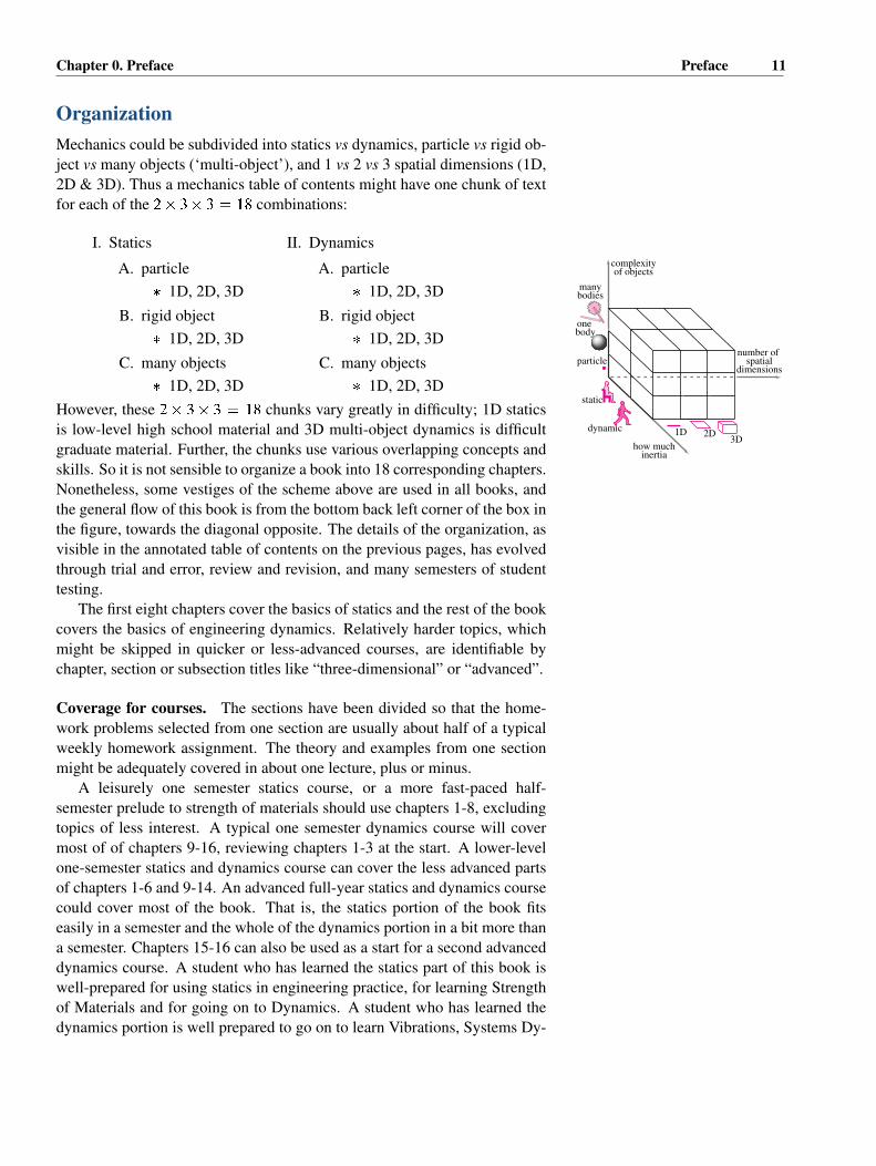
OrganizationMechanics could be subdivided into statics vs dynamics, particle vs rigid ob-ject vs many objects (‘multi-object’), and 1 vs 2 vs 3 spatial dimensions (1D,2D & 3D). Thus a mechanics table of contents might have one chunk of textfor each of the 2 � 3 � 3 D 18 combinations:

I. Statics

A. particle� 1D, 2D, 3D

B. rigid object� 1D, 2D, 3D

C. many objects� 1D, 2D, 3D

II. Dynamics

A. particle� 1D, 2D, 3D

B. rigid object� 1D, 2D, 3D

C. many objects� 1D, 2D, 3D

However, these 2 � 3 � 3 D 18 chunks vary greatly in difficulty; 1D staticsis low-level high school material and 3D multi-object dynamics is difficultgraduate material. Further, the chunks use various overlapping concepts andskills. So it is not sensible to organize a book into 18 corresponding chapters.Nonetheless, some vestiges of the scheme above are used in all books, andthe general flow of this book is from the bottom back left corner of the box inthe figure, towards the diagonal opposite. The details of the organization, asvisible in the annotated table of contents on the previous pages, has evolvedthrough trial and error, review and revision, and many semesters of studenttesting.

The first eight chapters cover the basics of statics and the rest of the bookcovers the basics of engineering dynamics. Relatively harder topics, whichmight be skipped in quicker or less-advanced courses, are identifiable bychapter, section or subsection titles like “three-dimensional” or “advanced”.

Coverage for courses. The sections have been divided so that the home-work problems selected from one section are usually about half of a typicalweekly homework assignment. The theory and examples from one sectionmight be adequately covered in about one lecture, plus or minus.

A leisurely one semester statics course, or a more fast-paced half-semester prelude to strength of materials should use chapters 1-8, excludingtopics of less interest. A typical one semester dynamics course will covermost of of chapters 9-16, reviewing chapters 1-3 at the start. A lower-levelone-semester statics and dynamics course can cover the less advanced partsof chapters 1-6 and 9-14. An advanced full-year statics and dynamics coursecould cover most of the book. That is, the statics portion of the book fitseasily in a semester and the whole of the dynamics portion in a bit more thana semester. Chapters 15-16 can also be used as a start for a second advanceddynamics course. A student who has learned the statics part of this book iswell-prepared for using statics in engineering practice, for learning Strengthof Materials and for going on to Dynamics. A student who has learned thedynamics portion is well prepared to go on to learn Vibrations, Systems Dy-

complexity of objects

number of spatial

dimensions

how much inertia

1D 2D3D

static

dynamic

particle

many bodies

one body

12 Chapter 0. Preface Preface

1 For example, we use angularmomentum balance (appropriatelyexpressed) with respect to any possibly-accelerating point, not just pointsselected from an arcane list.

namics or more advanced Multi-object Dynamics.

Organization and formatting

Each subject is covered in various ways.

� Every section starts with descriptive text and short examples motivat-ing and describing the theory;

� More detailed explanations of the theory are in boxes interspersed inthe text. For example, one box explains the common derivation of an-gular momentum balance from

*

F D m*a (page 974), one explains the

genius of the wheel (page 208), and another connects *! based kine-

matics to Oer and Oe� based kinematics (page 856);

� Sample problems (marked with a gray border) at the end of each sec-tion show how to do homework-like calculations. These set an exampleby their consistent use of free-body diagrams, systematic applicationof basic principles, vector notation, units, and checks against both in-tuition and special cases;

� Homework problems at the end of each chapter give students a chanceto practice mechanics calculations. The first problems for each sectionbuild a student’s confidence with the basic ideas. The problems areranked in approximate order of difficulty, with theoretical problemscoming later. Problems marked with a * have an answer at the backof the book;

� Reference tables on the inside covers and end pages concisely sum-marize much of the content in the book. These tables can save studentsthe time of hunting for formulas and definitions.

Notation

Clear vector notation helps students do problems. One common class ofstudent errors comes from copying a textbook’s printed bold vector F thesame way as a plain-text scalar F . We reduce this error by use a redundantvector notation, a bold and harpooned

*

F .As for all authors and teachers concerned with motion in two and three

dimensions we have struggled with the tradeoffs between a precise notationand a simple notation. Perfectly precise notations are complex and intimidat-ing. Simple notations are ambiguous and hide key information. Our attemptat clarity without too-much clutter is summarized in the box on page 40.

Relation to other mechanics booksThe bulk of the content of this book can be found in other places includ-ing freshman physics texts, other engineering texts, and hundreds of clas-sics. Nonetheless this book is in some ways different in organization and ap-proach. It also uses some important but not well-enough known concepts 1 .Mastery of freshman physics (e.g., from Halliday, Resnick & Walker, Tipler,

Chapter 0. Preface Preface 13

or Serway) would encompass some of this book’s contents. However, afterfreshman physics students often have only a vague notion of what mechan-ics is, and how it can be used. For example many students leave freshmanphysics with the sense that a free-body diagram (or ‘force diagram’) is avague conceptual picture with arrows for various forces and motions drawnon it this way and that. Even the freshman-text illustrations sometimes do notmake clear which force is acting on which object. Also, because freshmanphysics tends to avoid use of college math, many students leave freshmanphysics with little sense of how to use vectors or calculus to solve mechanicsproblems. This book aims to lead students who may start with these fuzzyfreshman-physics notions into a world of precise, yet still intuitive, mechan-ics.

Various statics and dynamics textbooks cover much of the same materialas this one. These textbooks have modern applications, ample samples, lotsof pictures, and lots of homework problems. Many are excellent in someways. Most of today’s engineering professors learned from one of thesebooks. Nonetheless we wrote this book hoping to do still better. Some ofour goals include

� showing the unity of the subject,� presenting a complete description of the subject,� clear notation in figures and equations,� integration of the applicability of computers,� consistent use of units throughout,� introduction of various insights into how things work,� a friendly writing style.

Between about 1689 and 1960 hundreds of books were written with ti-tles like Statics, Engineering mechanics, Dynamics, Machines, Mechanisms,Kinematics, or Elementary physics. Many thoughtfully cover most of thematerial here and sometimes much more. But none are good modern text-books; they lack an appropriate pace, style and organization; they are tooreliant on geometry skills and not enough on vectors and numerics; and theydon’t have enough modern applications, samples calculations, illustrations,or homework problems. But much good mechanics can be found only inthese older books 2 . If you love mechanics you will enjoy pondering ideasin some of these books.

What do you think?We have tried to make it as easy as possible for you to learn basic mechanicsfrom this book. We present truth as we know it and as we think it is effec-tively communicated. Nonetheless we have surely made some technical andstrategic errors. Please let us know your thoughts so that we can improvefuture editions.

Rudra Pratap, [email protected] Ruina, [email protected]

2 Here are three good and universallyrespected classics:

J.P. Den Hartog’s Mechanics orig-inally published in 1948 but stillavailable as an inexpensive reprint (wellwritten and insightful);

J.L. Synge and B.A. Griffith, Principlesof Mechanics through page 408. Orig-inally published in 1942, reprinted in1959 (good pedagogy but dry); and

E.J. Routh’s, Dynamics of a Sys-tem of rigid bodies, Vol 1 (the“elementary” part through chapter 7.Originally published in 1905, butreprinted in 1960). Routh also has 5other idea- packed statics and dynamicsbooks. Routh shared college gradua-tion honors with the now-more-famousphysicist James Clerk Maxwell.

14 Chapter 0. Preface 0.1. To the student (please read)

1 “Exams are harder than home-work.” Some struggling students say “Ican do the homework problems. I justcan’t do the exams. Exams are harderand trickier.” These students may befooling themselves. Most exams are nottrickier than the homework. And whenwe have checked, many students whogot through homework with help, can’tdo simplified versions of those sameproblems when they have no help.

0.1 To the student (please read)Nature’s rules are so strict that, to the extent that you know the rules, you canmake reliable predictions about how Nature, the set of all things, behave. Inparticular, most objects of concern to engineers obediently follow a subset ofNature’s rules called the laws of Newtonian mechanics. So, if you learn thelaws of mechanics, as this book should help you to do, you will be able tomake quantitative predictions about how things stand, move, and fall. Andyou will gain intuition about the mechanics part of Nature’s rules.

How to use this bookHere is some general guidance.

Check your own understanding

Most likely you want a decent grade by successfully getting through thehomework assignements and exams. You will naturally get help by lookingat examples and samples in the text or lecture notes, by looking up formulasin the front and back covers of this book, and by asking questions of friends,teaching assistants and professors. What good are books, notes, classmatesor teachers if they don’t help you do the homework? All the examples andsample problems in this book, for example, are just for this purpose.

But watch out. Too-much use of help from books, notes and people canlead to self deception 1 . After you have got through a problem using suchhelp you should, at least sometimes, check that you have actually learned tosolve the problem.

To see if you have learned to do a problem, do it again, justifying eachstep, without looking up even one small (‘oh, I almost knew that’) thing.

If you can’t do this, you gain two learning opportunities. First, you can learnthe missing skill or idea. But more deeply, by getting stuck after you havebeen able to get through with help, you can learn things about your learningprocess. Often the real source of difficulty isn’t a key formula or fact, butsomething more subtle. Some useful more subtle ideas might be explainedin the general text discussions.

Read the parts that are at your level

You might be science and math school-smart, mechanically inclined, or areespecially motivated to learn mechanics. Or you might be reluctantly takingthis class to fulfil a requirement. In either case this book is meant for you.The sections start with generally accessible introductory material and includesimple examples. The early sample problems in each section are also easy.But we also have discussions of the theory and other more advanced appli-cations and asides to challenge more motivated students. If you are a nerd,

Chapter 0. Preface 0.1. To the student (please read) 15

please be patient with the slow introductions and the calculations that go lineby line without skipping steps. On the other hand, if you are just trying toget through this course you need not stop and admire every side discussionabout history or theory.

Calculation strategies and skillsWe try to demonstrate a systematic approach to solving problems. But itsimpossible to reduce all mechanics problem solutions to one clear recipe (de-spite the generally applicable recipe on the inside back cover). If a preciserecipe existed then someone could write a computer program that followedit, and we would not have written this textbook. Your mind could be freedfrom mechanics problem solutions like a calculator frees you from the te-dium of long division. But there is an art to solving mechanics problems andunderstanding their solutions. This applies to homework problems and alsoengineering design problems. Art and human insight, as opposed to precisealgorithm or recipe, is what makes engineering require humans and not justcomputers 2 . We will try to teach you some of this art. For starters, here aresome tips.

Understand the question

It is tempting to start writing equations and quoting principles when you firstsee a problem. However, it is usually worth a few minutes (and sometimesa few hours) to try to get an intuitive sense of a problem before jumping toequations. Before you draw any sketches or write equations, think: does theproblem make sense? What information has been given? What are you tryingto find? Is what you are trying to find determined by what is given? Whatphysical laws make the problem solvable? What extra information do youthink you need? What information have you been given that you don’t need?You should first get a general sense of the problem to steer you through thetechnical details.

Some students find they can read every line of sample problems yet can-not do test problems, or, later on, cannot do applied design work effectively.This failing may come from following details without spending time, think-ing and gaining an overall sense of the problems.

Think through your solution strategy

For problem solutions you read, like those in this book, someone had to thinkabout the order of work. You also have to think about the order of your work.You will find some tips in the text and samples. But it is your job to own thematerial, to learn how to think about it your own way, to become an expert inyour own style, and to do the work in the way that makes things most clearto you and your readers.

2 Computers can do dynamics. To behonest, this book presents some meth-ods which computers can handle. Oncea problem has been reduced to a pre-cise mechanical model a computer codecould take over. Say a finite-elementprogram or a rigid-body dynamics pro-gram. But you will do better at me-chanics, even with a computers help, ifyou can do simple mechanics problemswithout a computer.Analogy with long-division. Sinceabout 1975 division by a 3 (or more)digit number is done by calculators,not pencil-and-paper long-division. Butcompetence at division without a calcu-lator, at least at division by one digitnumbers, allows one to quickly catchcalculator-entry errors. And knowledgeabout division (that, for example, its in-verse multiplication, or that division byzero is bad) is useful. And such knowl-edge comes better by practice with num-bers manipulated in one’s head and onpaper than just on a calculator. Sim-ilarly it is useful to know mechanics-problem methods well, even if some ofthose problems can be solved with by acomputer package.

16 Chapter 0. Preface 0.1. To the student (please read)

3 A tree analogy. Energy gets storedin the roots of a tree. It gets there fromthe trunk. The branches feed the trunk,the twigs feed the branches, and theleaves feed the twigs with energy fromthe sun. But the flow goes the oppo-site way, from the leaves on down to theroots. But if you try to invent a tree bystarting at the leaves with no knowledgeof the root you could easily get lost andconnect leaves to electric wires or gaspipes — all nonsense. There’s no pointin connecting the leaves to anything un-til you have a sense of the whole tree.

The order of calculation is often backwards from the order ofthinking

When working out how to solve a problem you often start with general prin-ciples, then look at terms you need to know. If these are not given, you thinkhow to figure those from other terms and so on. On the other hand, when yougo to calculate an answer you have to start with the information given andwork your way backwards into the equation which has your answer 3 . Tofind the net worth of a corporation you add the value of the various divisions.To get the value of a division you add up the values of the factories. For eachfactory you add up the value of the pieces of machinery. But to get an ac-tual corporate value you have to start by evaluating the pieces of machineryin each factory and working back up from the known towards the answer.Beware that

When you read the minimal write-up of a calculation, especially analgorithmic recipe or computer program, you often are reading in theinverse order of the thinking that went in to generating the solution.

Of course real problem solving goes both ways. You think about what youneed in order to calculate what you want. But you also think about what youcan calculate easily from what is given plainly to you. You reach from thebroad towards the details. And you work with known details towards answersof any kind, wanted or not. And you thus hunt out, building from details andsimultaneously reaching back from the goal, a route leading all the way fromthe details to the goal.

Look for equations containing unkowns, not for formulas thatevaluate unknowns

In elementary science and math we often learn formulas like

V D LWH; d D 1

2at2; and x D �b �

pb2 � 4ac

2a

to find V; d; or x. So it is common wishful thinking for newcomers to hopefor a formula that generates the sought unknown in terms of given quantities.Rather, you should

Find relations that contain variables of interest; don’t worry aboutwhether they are on the right or left side of an equation. Don’t worryabout whether the variables are alone or isolated.

Most often, you will not know a formula where the thing you want is on theleft and everything given is on the right. You will have, say,

V D LWH when you want to find W from V;L; and H ,

Chapter 0. Preface 0.1. To the student (please read) 17

d D 1

2at2 when you want to find t from a and d , and

ax2 C bx C c D 0 when you want to find x from a; b; and c.

Once you have got this far the only problem is math 4 . Here are two tricksof the mind

1) You know a math and computer genius. She is helpful but doesn’tknow any mechanics. Make your first task writing things down so shecould finish up for you. She doesn’t want to help? Then realize thatfinishing up without her is a separate job for you. You will do this laterwhen you wear your math-genius cap.

2) Be an egotist. Pretend you are omniscient and know everything. Thenwrite down true statements about those things; equations that containterms that omniscient-you already know: “If I knew x; y and z thefollowing equation would be true.” Then relax your ego a bit. Countequations and unknowns to see if you, or at least your math geniusfriend, could solve for the things you previously pretended to know.

Vectors and free-body diagramsIn the toolbox of someone who can solve lots of mechanics problems are twowell-worn tools:

� A vector calculator that always keeps vectors and scalars distinct, and

� A reliable and clear free-body diagram drawing tool.

Because many of the terms in mechanics equations are vectors, the ability todo vector calculations is essential. Because the concept of an isolated systemis at the core of mechanics, every mechanics practitioner needs the ability todraw a good free-body diagram. The second and third chapters will help youbuild your own set of these two most-important tools.

Guarantee: If you learn to do clear correct vector algebra and to drawgood free-body diagrams you will do well at mechanics. (Assuming, ofcourse, that you don’t totally stop studying then and there.)

Thinking outside the booksWe do mechanics because we like mechanics. We hope you will too. It’s funto puzzle out how things work. Its satisfying to do calculations that makerealistic predictions. Mechanics is interesting in its own right and it feelsgood to take pride in new skills. We wrote this book because we want to helpyou learn the subject if you are interested, and get through it if you must.But we don’t know a straightforward path through your resources (say a pathwith 4 straight segments) that really gets you to deeper understanding.

4 For this and other courses, youshould be good at solving math prob-lems with your pencil and with a com-puter. But you should distinguish be-tween the task of setting up a math prob-lem and the solving of the problem.The solving often takes the bulk of thetime and paper, but it’s not where yourthoughts should start. The material thatis new for you in this book is largelyabout setting up, rather than solving, themath problems that arrise in mechanics.

Filename:tfigure-outsidethebooks

Dynamics

Math

Backspace CE C

Outside the books

The books

Statics

Engineering

254

Figure 0.1: Thinking outside of thebooks. A famous puzzle asks: using4 contiguous straightline segments con-nect all 9 dots that are in a square 3 � 3array. The only solution has segmentsextending outside the “box” of 9 points.Hence the expression “thinking outsideof the box”.

18 Chapter 0. Preface 0.2. A note on computation

We do know that you need to think outside of the confines of your usualstudy resources. Like when you are relaxed, away from the pressures ofbooks, notes, pencils or paper, say when you are walking, showering or lyingdown. These are the places where you naturally work out life problems, butthey are good places to work out mechanics problems too.

Having an animated mechanics discussion with friends is also good. Youshould enjoy your inner nerd socially. Are your friends turned off by tech-talk? There are billions of people out there, you should be able to find one ortwo that like to talk shop.

0.2 A note on computationMechanics is a physical subject. The concepts in mechanics do not dependon computers. But mechanics is also a quantitative subject; relevant amounts(of length, mass, force, moment, time, etc) are described with numbers, andrelations are described using equations and formulas. Computers are verygood with numbers and formulas. Thus the modern practice of engineeringmechanics uses computers. The most-needed computer skills for mechanicsare:

� solution of simultaneous linear algebraic equations,

� plotting, and

� numerical solution of ODEs (Ordinary Differential Equations).

More basically, an engineer also needs the ability to routinely evaluate stan-dard functions (x3, cos�1 � , etc.), to enter and manipulate lists and arrays ofnumbers, and to write short programs.

Classical languages, applied packages, and simulators

Programming in standard languages such as Fortran, Basic, Pascal, C++, orJava probably take too much time to use in solving simple mechanics prob-lems. Thus an engineer needs to learn to use one or another widely avail-able computational package (e.g., MATLAB, O-MATRIX, SCI-LAB, OC-TAVE, MAPLE, MATHEMATICA, MATHCAD, TKSOLVER, LABVIEW,etc). We assume that students have learned, or are learning such a pack-age. Although none of the homework here depends on such, we also en-courage you to play with packaged mechanics simulators (e.g., INVENTOR,WORKING MODEL, ADAMS, DADS, ODE, etc) for testing and buildingyour intuition.

How we explain computation in this book.

Solving a mechanics problem involves1. Reducing a physical problem to a well posed mathematical problem;

2. Solving the math problem using some combination of pencil and paperand numerical computation; and

Chapter 0. Preface 0.2. A note on computation 19

3. Giving physical interpretation of the mathematical solution.This book is primarily about setup (a) and interpretation (c), which are ratherthe same, no matter what method is used to solve the equations. If a problemrequires computation, the exact computer commands vary from package topackage. And we don’t know which one you are using. So in this bookwe express our computer calculations using an informal pseudo computerlanguage. For reference, typical commands are summarized on page 21.

Required computer skills

Here, in a little more detail, are the primary computer skills you need.

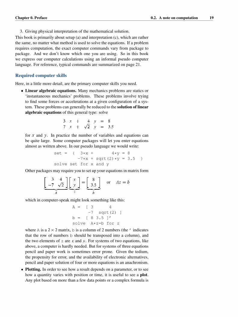
� Linear algebraic equations. Many mechanics problems are statics or‘instantaneous mechanics’ problems. These problems involve tryingto find some forces or accelerations at a given configuration of a sys-tem. These problems can generally be reduced to the solution of linearalgebraic equations of this general type: solve

3 x C 4 y D 8

�7 x C p2 y D 3:5

for x and y. In practice the number of variables and equations canbe quite large. Some computer packages will let you enter equationsalmost as written above. In our pseudo language we would write:

set = { 3*x + 4*y = 8-7*x + sqrt(2)*y = 3.5 }

solve set for x and y

Other packages may require you to set up your equations in matrix form�3 4

�7 p2

��

A

�x

y

��z

D�

8

3:5

��

b

or Az D b

which in computer-speak might look something like this:

A = [ 3 4-7 sqrt(2) ]

b = [ 8 3.5 ]’solve A*z=b for z

where A is a 2 � 2 matrix, b is a column of 2 numbers (the ’ indicatesthat the row of numbers b should be transposed into a column), andthe two elements of z are x and y. For systems of two equations, likeabove, a computer is hardly needed. But for systems of three equationspencil and paper work is sometimes error prone. Given the tedium,the propensity for error, and the availability of electronic alternatives,pencil and paper solution of four or more equations is an anachronism.

� Plotting. In order to see how a result depends on a parameter, or to seehow a quantity varies with position or time, it is useful to see a plot.Any plot based on more than a few data points or a complex formula is

20 Chapter 0. Preface 0.2. A note on computation

far more easily drawn using a computer than by hand. Most often youcan organize your data into a set of .x; y/ pairs stored in an x list and acorresponding y list. A simple computer command will then plot x vsy. The pseudo-code below, for example, plots a circle using 100 points

npoints = [0 1 2 3 ... 100]theta = npoints * 2 * pi / 100x = cos(theta)y = sin(theta)plot y vs x

where npoints is the list of numbers from 1 to 100, theta is a listof 100 numbers evenly spaced between 0 and 2� and x and y are listsof 100 corresponding x; y coordinate points on a circle.

� ODEs The result of using the laws of dynamics is often a set of differ-ential equations which need to be solved. A simple example would be:

Find x at t D 5 given thatdx

dtD x and that at t D 0, x D 1.

The solution to this problem can be found easily enough by hand tobe x.5/ D e5. But often the differential equations are just too hard forpencil and paper solution. Fortunately the numerical solution of ordi-nary differential equations (ODEs) is already programmed into sci-entific and engineering computer packages. The simple problem aboveis solved with computer code equivalent to these informal commands:

ODES = { xdot = x }ICS = { xzero = 1 }solve ODES with ICS until t=5

which will yield a list of values for paired values for t and x the last ofwhich will be t D 5 and x close to e5 � 148:4.

Chapter 0. Preface 0.2. A note on computation 21

Examples of informal computer commandsIn this book computer commands are given informally using com-mands that are not as strict as any real computer package. You willneed to translate the informal commands below into commands yourpackage understands. This reference table uses mathematical ideaswhich you may or may not know before you read this book, but theseare introduced in the text when needed.. . . . . . . . . . . . . . . . . . . . . . . . . . . . . . . . . . . . . . . . . . . . . . . . . . . . . . . . . . . . .x=7 Set the variable x to 7.. . . . . . . . . . . . . . . . . . . . . . . . . . . . . . . . . . . . . . . . . . . . . . . . . . . . . . . . . . . . .omega=13 Set ! to 13.. . . . . . . . . . . . . . . . . . . . . . . . . . . . . . . . . . . . . . . . . . . . . . . . . . . . . . . . . . . . .u=[1 0 -1 0]v=[2 3 4 pi]

Define u and v to be the listsshown.

. . . . . . . . . . . . . . . . . . . . . . . . . . . . . . . . . . . . . . . . . . . . . . . . . . . . . . . . . . . . .t= [.1 .2 .3 ... 5] Set t to the list of 50 numbers

implied by the expression.. . . . . . . . . . . . . . . . . . . . . . . . . . . . . . . . . . . . . . . . . . . . . . . . . . . . . . . . . . . . .y=v(3) sets y to the third value of v (in

this case 4).. . . . . . . . . . . . . . . . . . . . . . . . . . . . . . . . . . . . . . . . . . . . . . . . . . . . . . . . . . . . .A=[1 2 3 6.9

5 0 1 12 ]Set A to the array shown.

. . . . . . . . . . . . . . . . . . . . . . . . . . . . . . . . . . . . . . . . . . . . . . . . . . . . . . . . . . . . .z= A(2,3) Set z to the element of A in the

second row and third column.. . . . . . . . . . . . . . . . . . . . . . . . . . . . . . . . . . . . . . . . . . . . . . . . . . . . . . . . . . . . .w=[3

425]

Define w to be a column vector.

. . . . . . . . . . . . . . . . . . . . . . . . . . . . . . . . . . . . . . . . . . . . . . . . . . . . . . . . . . . . .w = [3 4 2 5]’ Same as above. ’ means

transpose.. . . . . . . . . . . . . . . . . . . . . . . . . . . . . . . . . . . . . . . . . . . . . . . . . . . . . . . . . . . . .u+v Vector addition. In this case the

result is �3 3 3 ��.. . . . . . . . . . . . . . . . . . . . . . . . . . . . . . . . . . . . . . . . . . . . . . . . . . . . . . . . . . . . .u*v Element by element

multiplication, in this case�2 0 � 4 0�.

. . . . . . . . . . . . . . . . . . . . . . . . . . . . . . . . . . . . . . . . . . . . . . . . . . . . . . . . . . . . .sum(w) Add the elements of w , in this

case 14.. . . . . . . . . . . . . . . . . . . . . . . . . . . . . . . . . . . . . . . . . . . . . . . . . . . . . . . . . . . . .cos(w) Make a new list, each element of

which is the cosine of thecorresponding element of �w�.

. . . . . . . . . . . . . . . . . . . . . . . . . . . . . . . . . . . . . . . . . . . . . . . . . . . . . . . . . . . . .

mag(u) The square root of the sum of thesquares of the elements in �u�, inthis case 1.41421...

. . . . . . . . . . . . . . . . . . . . . . . . . . . . . . . . . . . . . . . . . . . . . . . . . . . . . . . . . . . . .u dot v The vector dot product of

component lists �u� and �v�, (wecould also write sum(A*B).

. . . . . . . . . . . . . . . . . . . . . . . . . . . . . . . . . . . . . . . . . . . . . . . . . . . . . . . . . . . . .

C cross D The vector cross product of*C

and*D, assuming the three

element component lists for �C �and �D� have been defined.

. . . . . . . . . . . . . . . . . . . . . . . . . . . . . . . . . . . . . . . . . . . . . . . . . . . . . . . . . . . . .A matmult w Use the rules of matrix

multiplication to multiply �A�and �w�.

. . . . . . . . . . . . . . . . . . . . . . . . . . . . . . . . . . . . . . . . . . . . . . . . . . . . . . . . . . . . .eqset = f3x + 2y = 6

6x + 7y = 8gDefine ‘eqset’ to stand for the setof 2 equations in braces.

. . . . . . . . . . . . . . . . . . . . . . . . . . . . . . . . . . . . . . . . . . . . . . . . . . . . . . . . . . . . .solve eqset

for x and ySolve the equations in ‘eqset’ forx and y.

. . . . . . . . . . . . . . . . . . . . . . . . . . . . . . . . . . . . . . . . . . . . . . . . . . . . . . . . . . . . .solve Ax=b for x Solve the matrix equation

�A��x� D �b� for the list ofnumbers x. This assumes A andb have already been defined.

. . . . . . . . . . . . . . . . . . . . . . . . . . . . . . . . . . . . . . . . . . . . . . . . . . . . . . . . . . . . .for i = 1 to N

such and suchend

Execute the commands ‘such andsuch’N times, the first time withi D 1, the second with i D 2, etc

. . . . . . . . . . . . . . . . . . . . . . . . . . . . . . . . . . . . . . . . . . . . . . . . . . . . . . . . . . . . .plot y vs x Assuming x and y are two lists

of numbers of the same length,plot the y values vs the x values.

. . . . . . . . . . . . . . . . . . . . . . . . . . . . . . . . . . . . . . . . . . . . . . . . . . . . . . . . . . . . .solve ODEswith ICsuntil t=5

Assuming a set of ODEs and ICshave been defined, use numericalintegration to solve them andevaluate the result at t D 5.

. . . . . . . . . . . . . . . . . . . . . . . . . . . . . . . . . . . . . . . . . . . . . . . . . . . . . . . . . . . . .

With an informality consistent with what is written above, othercommands are introduced as needed.

introduction to tatics ynamics - andy...

Documents