introduction to the essentials of tensor calculusphy315/tensors.pdf · introduction to the...

1

INTRODUCTION TO THE ESSENTIALS OF TENSOR CALCULUS

********************************************************************************I. Basic Principles ..... . . . . . . . . . . . . . . . . . . . . . . . . . . . . . . . . . . . . . . . . . . . . . . . . . . . . . . . . . . . . . . . . . 1II. Three Dimensional Spaces ..... . . . . . . . . . . . . . . . . . . . . . . . . . . . . . . . . . . . . . . . . . . . . . . . . . . . . . . . . 4III. Physical Vectors .... . . . . . . . . . . . . . . . . . . . . . . . . . . . . . . . . . . . . . . . . . . . . . . . . . . . . . . . . . . . . . . . . . . 8IV. Examples: Cylindrical and Spherical Coordinates.... . . . . . . . . . . . . . . . . . . . . . . . . . . . . . . 9V. Application: Special Relativity, including Electromagnetism.... . . . . . . . . . . . . . . . . . . . . . 10VI. Covariant Differentiation ............................................................. 17VII. Geodesics and Lagrangians............................................................. 21********************************************************************************

I. Basic PrinciplesWe shall treat only the basic ideas, which will suffice for much of physics. The objective is to

analyze problems in any coordinate system, the variables of which are expressed as

qj(xi) or q'j(qi) where xi : Cartesian coordinates, i = 1,2,3, ....N

for any dimension N. Often N=3, but in special relativity, N=4, and the results apply in anydimension. Any well-defined set of qj will do. Some explicit requirements will be specified later.

An invariant is the same in any system of coordinates. A vector, however, has componentswhich depend upon the system chosen. To determine how the components change (transform) withsystem, we choose a prototypical vector, a small displacement dxi. (Of course, a vector is ageometrical object which is, in some sense, independent of coordinate system, but since it can beprescribed or quantified only as components in each particular coordinate system, the approach here isthe most straightforward.) By the chain rule, dqi = ( ∂qi / ∂xj ) dxj , where we use the famoussummation convention of tensor calculus: each repeated index in an expression, here j, is to besummed from 1 to N. The relation above gives a prescription for transforming the (contravariant)vector dxi to another system. This establishes the rule for transforming any contravariant vector fromone system to another.

Ai (q) = ( ∂qi

∂xj ) Aj (x)

Ai(q') = ( ∂q'i

∂qj ) Aj(q) = ( ∂q'i

∂qj ) ( ∂qj

∂xk ) Ak(x) ≡ ( ∂q'i

∂xk ) Ak(x)

Λij (q,x) ≡ ∂qi

∂xj Contravariant vector transform

The (contravariant) vector is a mathematical object whose representation in terms of componentstransforms according to this rule. The conventional notation represents only the object, Ak, withoutindicating the coordinate system. To clarify this discussion of transformations, the coordinate systemwill be indicated by Ak(x), but this should not be misunderstood as implying that the components inthe "x" system are actually expressed as functions of the xi. (The choice of variables to be used toexpress the results is totally independent of the choice coordinate system in which to express thecomponents Ak. The Ak(q) might still be expressed in terms of the xi, or Ak(x) might be moreconveniently expressed in terms of some qi.)

Distance is the prototypical invariant. In Cartesian coordinates, ds2 = δij dxi dxj , where

δij is the Kroneker delta: unity if i=j, 0 otherwise. Using the chain rule,


2

dxi = ( ∂xi

∂qj ) dqj

ds2 = δij ( ∂xi

∂qk ) ( ∂xj

∂ql ) dqk dql = gkl (q) dqk dql

gkl (q) ≡ ( ∂xi

∂qk ) ( ∂xj

∂ql ) δij (definition of the metric tensor)

One is thus led to a new object, the metric tensor, a (covariant) tensor, and by analogy, the covarianttransform coefficients:

Λji(q,x) ≡ ( ∂xj

∂qi ) Covariant vector transform

{More generally, one can introduce an arbitrary measure (a generalized notion of 'distance') ina chosen reference coordinate system by ds2 = gkl (0) dqk dql , and that measure will be invariant ifgkl transforms as a covariant tensor. A space having a measure is a metric space.}

Unfortunately, the preservation of an invariant has required two different transformation rules,and thus two types of vectors, covariant and contravariant, which transform by definition according tothe rules above. (The root of the problem is that our naive notion of 'vector' is simple and well-defined only in simple coordinate systems. The appropriate generalizations will all be developed indue course here.) Further, we define tensors as objects with arbitrary covariant and contravariantindices which transform in the manner of vectors with each index. For example,

Tijk(q) ≡ Λi

m (q,x) Λjn(q,x) Λl

k(q,x) Tmnl (x)

The metric tensor is a special tensor. First, note that distance is indeed invariant:

ds2(q') = gkl (q') dq'k dq'l

= ( ∂qi

∂q'k ) (

∂qj

∂q'l ) gij (q) (

∂q'k

∂qs ) dqs (

∂q'l

∂qt ) dqt

= gij (q) ( ∂qi

∂q'k )(

∂q'k

∂qs ) (

∂qj

∂q'l )(

∂q'l

∂qt ) dqs dqt

⇓ ⇓∂qi

∂qs = δis δjt

= gij (q) dqi dqj ≡ ds2(q)

There is also a consistent and unique relation between the covariant and contravariantcomponents of a vector. (There is indeed a single 'object' with two representations in each coordinatesystem.)

dqj ≡ gji dqi


3

dq'j ≡ gji (q') dq'i = gkl (q) ( ∂qk

∂q'j ) (

∂ql ∂q'i

) (∂q'i

∂qp ) dqp

⇓ δlp

= ( ∂qk

∂q'j ) gkl (q) dql = (

∂qk

∂q'j ) dqk

Thus it transforms properly as a covariant vector.These results are quite general; summing on an index (contraction) produces a new object

which is a tensor of lower rank (fewer indices).

Tijk G

kl = R

ijl

The use of the metric tensor to convert contravariant to covariant indices can be generalized to'raise' and 'lower' indices in all cases. Since gij = δij in Cartesian coordinates, dxi =dxi ; there is

no difference between co- and contra-variant. Hence gij = δij , too, and one can thus define gij inother coordinates. {More generally, if an arbitrary measure and metric have been defined, thecomponents of the contravariant metric tensor may be found by inverting the [N(N+1)/2] equations(symmetric g) of gij (0) gik(0) gnj(0) = gkn(0). The matrices are inverses.}

Ai(q) ≡ gij (q) Aj(q)

gij = gik gkj = (

∂qi

∂xm ) ( ∂qk

∂xn ) δmn ( ∂xr

∂qk ) ( ∂xs

∂qj ) δrs

| | ⇓ δrn

= ( ∂qi

∂xs ) ( ∂xs

∂qj ) = δij = δij

Thus gij is a unique tensor which is the same in all coordinates, and the Kroneker delta is sometimes

written as δij to indicate that it can indeed be regarded as a tensor itself.

Contraction of a pair of vectors leaves a tensor of rank 0, an invariant. Such a scalar invariantis indeed the same in all coordinates:

Ai(q')Bi(q') = ( ∂q'i

∂qj ) Aj(q) (

∂qk

∂q'i ) Bk(q) = δjk Aj(q) Bk(q)

= Aj(q) Bj(q)

It is therefore a suitable definition and generalization of the dot or scalar product of vectors.Unfortunately, many of the other operations of vector calculus are not so easily generalized.

The usual definitions and implementations have been developed for much less arbitrary coordinatesystems than the general ones allowed here.

For example, consider the gradient of a scalar. One can define the (covariant) derivative of ascalar as


4

Ø(x),i ≡ ∂Ø∂xi Ø(q),i ≡

∂Ø∂qi = (

∂Ø∂xj ) (

∂xj

∂qi )

The (covariant) derivative thus defined does indeed transform as a covariant vector. The commanotation is a conventional shorthand. {However, it does not provide a direct generalization of thegradient operator. The gradient has special properties as a directional derivative which presupposeorthogonal coordinates and use a measure of physical length along each (perpendicular) direction. Weshall return later to treat the restricted case of orthogonal coordinates and provide specialized results forsuch systems. All the usual formulas for generalized curvilinear coordinates are easily recovered inthis limit.} A (covariant) derivative may be defined more generally in tensor calculus; the commanotation is employed to indicate such an operator, which adds an index to the object operated upon, butthe operation is more complicated than simple differentiation if the object is not a scalar. We shall nottreat the more general object in this section, but we shall examine a few special cases below.

II. Three Dimensional SpacesFor many physical applications, measures of area and volume are required, not only the basic

measure of distance or length introduced above. Much of conventional vector calculus is concernedwith such matters. Although it is quite possible to develop these notions generally for anN-dimensional space, it is much easier and quite sufficient to restrict ourselves to three dimensions.The appropriate generalizations are straightforward, fairly easy to perceive, and readily found inmathematics texts, but rather cumbersome to treat.

For writing compact expressions for determinants and various other quantities, we introducethe permutation symbol, which in three dimensions is

eijk = 1 for i,j,k=1,2,3 or an even permutation thereof, i.e. 2,3,1 or 3,1,2-1 for i,j,k= an odd permutation, i.e. 1,3,2 or 2,1,3 or 3,2,1 0 otherwise, i.e. there is a repeated index: 1,1,3 etc.

The determinant of a 3x3 matrix can be written as

|a| = eijk a1i a2j a3k

Another useful relation for permutation symbols is

eijk eilm = δjl δkm - δjm δklFurthermore,

δijklmn = eijk elmn and δijk

ijk = 3!

where δijklmn is a multidimensional form of the Kroneker delta which is 0 except when ijk and lmn

are each distinct triplets. Then it is +1 if lmn is an even permutation of ijk, -1 if it is an oddpermutation. These symbols and conventions may seem awkward at first, but after some practice theybecome extremely useful tools for manipulations. Fairly complicated vector identities andrearrangements, as one often encounters in electromagnetism texts, are made comparatively simple.

Although the permutation symbol is not a tensor, two related objects are:

εijk = √ g eijk and εijk = 1

√ g eijk where g ≡ | gij |

with absolute value understood if the determinant in negative. This surprising result may be confirmedby noting that the expression for the determinant given above may also be written as


5

elmn |a| = eijk ali amj ank

which is certainly true for l,m,n=1,2,3, and a little thought will show it to be true in all cases. Thetransformation law for g may then be obtained as

elmn |g(q')| =eijk g(q')li g(q')mj g(q')nk

= e ijk ( ∂qp

∂q'l ) (

∂qq

∂q'i ) (

∂qr

∂q'm ) (

∂qs

∂q'j ) (

∂qu

∂q'n ) (

∂qv

∂q'k )

gpq(q) grs(q) guv (q) (tensor transform of metric tensors)

= eqsv

∂ q ∂q' (

∂qp

∂q'l ) (

∂qr

∂q'm ) (

∂qu

∂q'n ) gpq grs guv

(considering the terms with indices i,j,k)

= epru g(q)

∂ q ∂q' ( ∂qp / ∂q'l )( ∂qr / ∂q'm )( ∂qu / ∂q'n )

(considering the terms with indices q,s,v in constituting a determinant as above)

= elmn g(q)

∂ q ∂q'

2 (forming another determinant as above)

thus establishing that g transforms with the square of the Jacobian determinant. For the putativelycovariant form of the permutation tensor,

εijk (q') = √g(q) erst ( ∂qr

∂q'i ) (

∂qs

∂q'j ) (

∂qt

∂q'k )

= eijk

∂ q ∂q' √g(q) = eijk √g(q'), the form desired.

Raising indices in the usual way will produce the contravariant form by arguments similar to thoseapplied above.

The permutation tensors enable one to construct true vectors analogous to the familiar ones.The vector or cross product becomes

Ai = εijk Bj Ck

although again we have both co and contravariant forms.


6

The invariant measure of volume is easily constructed as

∆V = εijk dqi dqj dqk

(3!)

which is explicitly an invariant by construction and can be identified as volume in Cartesiancoordinates. ( This is a general method of argument in tensor calculus. If a result is stated as anequation between tensors [or vectors or scalars], if it can be proven or interpreted in any coordinatesystem, it is true for all. That is the power of tensor calculus and its general properties oftransformation between coordinates.)

Note that the application of this relation for ∆V in terms of dqi and transforming directly fromCartesian dxi gives immediately the familiar relation

∆V= J dq1dq2dq3 J =

∂ x∂q the Jacobian.

For the volume integrals of interest, note that ∫ I εijk dqi dqj dqk , for I invariant, is

invariant, but ∫ Tv εijk dqi dqj dqk is not a vector, because the transformation law for Tv ingeneral changes over the volume.

The operators of divergence and curl require more care. Just as the gradient has a directphysical significance, these operators are constructed to satisfy certain Green's theorems, Gauss' andStokes law. These must be preserved if their utility is to continue. One can prove a beautiful generaltheorem in spaces of arbitrary dimension, from which all common vector theorems are simplecorollaries, but the proof requires extensive formal preparation. Instead, we shall providestraightforward, if lengthy, proofs of the two specific results desired.

For Gauss' law, we require a relation which is a proper equation between invariants andfurther reduces to the usual result in Cartesian coordinates,

∫ div(Tm) εijk dqi dqj dqk

3 ! = ∫ Ti dSi

the choice dSi = εijk dqj dqk is explicitly a (covariant) vector, making the right integral invariant,and it gives the correct result in Cartesians. On the left, we require a suitable operator. We shall nextprove that

1

√ g ∂[ ]( )√ g Ti

∂qi

is such an invariant. It certainly gives the usual Cartesian divergence, but the inspiration for thisguess must remain obscure, for it is deep in the development of general covariant differentiation andChristofel symbols. Fortunately, that need not concern us. Proof that this expression is indeedinvariant requires proving that the form is the same in any two systems:

1

√ g ' ∂[ ]( )√ g ' T'i

∂qi =

1 √ g '

∂

( )√ g ' Tk (

∂qi

∂xk )

∂qi =

1

√ g ∂[ ]( )√ g Ti

∂xiwhere √ g' =

∂x

∂q √ g ≡ J √ g


7

as shown above, introducing J for the Jacobian determinant. The expression in the new coordinatescan then be written

1

J√ g

∂[ ]( )√ g Tk

∂qi J (

∂qi

∂xk ) + TkJ

∂

J

∂qi

∂xk

∂qi

where the first term is simply the desired expression in xi by the chain rule, and we must show thatthe second term, the portion in brackets [], is then zero. That term may be written

∂

∂x

∂q

∂ qi (

∂qi

∂xk ) + J ∂2 qi ∂xk ∂xl (

∂xl

∂qi )

and the first term converted using J' =

∂q

∂x = 1/J to ∂ J'-1

∂xk =

-J2 ∂

∂q

∂x

∂xk = -J2

∂q

∂x ∂2 qi ∂xk ∂xl (

∂xl

∂qi )

thereby canceling the second term and proving the assertion. The last step requires some algebra toconfirm, but it is straightforward using the methods used above for writing a determinant, consideringall the terms present, and inserting a

δij= (

∂qi

∂xs ) ( ∂xs

∂qj )

'(with appropriate choice of indices), the inverse of the usual procedure. The 'tensorial'form of the divergence theorem is therefore an equality of invariants:

∫ 1

√ g ∂[ ]( )√ g Tm

∂qm εijk

dqi dqj dqk 3! = ∫ Ti εijk dqj dqk

Furthermore, the familiar result, div(ØA) = Ødiv(A) + ∇ Ø⋅A , remains as

div(ØA) = Ødiv(A) + ∂Ø∂qi

Ai

Fortunately, Stokes theorem is somewhat easier; there is only one subtlety. The naivegeneralization is

∫εijk ∂Tk∂qj

εist dqs dqt = ∫ Ti dqi

which again obviously reduces to the usual result in Cartesian coordinates and would be explicitly agood 'tensor' equation between invariants if ∂Tk/∂qj were indeed a covariant tensor of rank two. It isnot, but the portion used in the equation above is. In general,


8

Rij = Rij +Rji

2 + Rij - Rji

2

the sum of a symmetric and antisymmetric part. For contractions with the anti-symmetric permutationsymbol as used above, only the anti-symmetric part contributes; replacing

∂Tk∂qj

=

∂Tk

∂qj -

∂Tj∂qk

2

is equivalent and gives the identical Cartesian reduction. The antisymmetric expression is easilyshown to be a tensor as follows:

Rij ≡ ∂Ti∂xj

- ∂Tj∂xi

and R'ij ≡ ∂T'i∂qj

- ∂T'j∂qi

but by the laws of tensor transformation, this should also be

R'ij = ∂

Tk(

∂xk∂qi

)

∂qj -

∂

Tk(

∂xk∂qj

)

∂qi = Rkl (

∂xk∂qi

) (∂xk∂qj

)

= (∂Tk∂qj

) (∂xk∂qi

) - (∂Tk∂qi

) (∂xk∂qj

) + Tk ∂2xk∂qj∂qi

- Tk ∂2xk∂qi∂qj

where the last two terms cancel and the first two, using the chain rule (∂/∂qi)=(∂/∂xk)(∂xk/∂qi), givethe required tensor transform of Rij . We therefore have the desired tensor form of the divergence andcurl operators and the corresponding integral theorems. Note also that the important results curl ( gradØ) = 0 and div ( curl Ai) = 0 both follow easily from these forms by symmetry

eijk ∂2∂qi∂qj

= 0.

III. Physical Vectors

The distinction between covariant and contravariant vectors is essential to tensor analysis, but itis a complication which is unnecessary for elementary vector calculus. In fact, the usual formulationof vector calculus can be obtained from tensor calculus as a special case, that being one in which thecoordinate system is orthogonal. Most practical coordinate systems are of this type, for which tensoranalysis is not really necessary, but a few are not. (For example, in plasma physics, the naturalcoordinates may be ones determined by the magnetic geometry and not be orthogonal.) In orthogonalsystems with positive metric, one can define 'physical' vectors, which are neither covariant norcontravariant. Nevertheless, they have well-defined transformation properties among orthogonalsystems, and they have simple physical significance. For example, all components of a displacementvector have the dimensions of length. They are the vectors of traditional vector calculus. Fororthogonal systems of this type,

gij = h2i δij (hi is not a vector; no summation)


9

A(i) ≡ hi Ai = Aihi

(no summation)

for the components of the 'physical' vector. The usual dot or scalar product is simply A(i)A(i) andproduces the same result as given above. (In this special case, the metric tensor can be 'put into' thevector in a natural manner.)

All the usual vector formulas can be obtained from the preceding tensor expressions byconsistently converting to physical vectors. Note that g = (h1h2h3)2 and εijk = h eijk , using h =(h1h2h3).

C(i) = A(j) X B(k) = eijk A(j) B(k)

(grad Ø)(i) =(1/hi )(∂ Ø/∂qi)

div A = (1/h){∂[hA(i)/hi]/∂qi}

(curl A)(i) = (hi/h) eijk ∂[hkA(k)]/∂qj

Volume: (d3v) = h eijk dqidqjdqk = d3l = eijk dlidljdlk

Integrations are over physical volumes, areas, and lengths. If the integrals are set up in coordinateslike dq, the necessary factors must be inserted to give the physical units as illustrated here for volume.

IV. Examples

Cylindrical coordinatesA simple example to illustrate the ideas is provided by cylindrical coordinates:

x = r cos θ r = √x2 + y2

y = r sin θ θ = tan−1 (y/x)z = z

i \ j = 1 2 3

Λij ≡ ∂qi

∂xj =

cos θ sin θ 0

-(sin θ)/r (cos θ)/r 00 0 1

i \ j

Λji ≡ ∂xj

∂qi =

cos θ sin θ 0

-r(sin θ) r(cos θ) 00 0 1

gij =

1 0 0

0 r2 00 0 1

gij =

1 0 0

0 r-2 00 0 1

g = r2 hi = (1,r,1)


10

Spherical CoordinatesA second example of broad utility is spherical coordinates:

x = r sin θ cos φ r = √x2 + y2 + z2

y = r sin θ sin φ θ = tan-1

√x2 + y2

z

z = r cos θ φ = tan -1(y/x)

Λij ≡ ∂qi

∂xj =

sin θ cos φ sin θ sin φ cos θ

(cos θ cos φ)/r (cos θ sin φ)/r -(sin θ)/r

-sin φr sin θ

cos φr sin θ

0

i \ j

Λji ≡ ∂xj

∂qi =

sin θ cos φ sin θ sin φ cos θ

r cos θ cos φ r cos θ sin φ -r sin θ-r sin θ sin φ r sin θ cos φ 0

gij =

1 0 0

0 r2 00 0 r2sin2θ

gij =

1 0 0

0 r-2 00 0 r-2sin-2θ

g = r4 sin2 θ hi = (1,r,r sin θ) h = r2sin θ

V. Application: Special Relativity

Special relativity is generally introduced without tensor calculus, but the results often seemrather ad hoc. Einstein used the ideas of tensor calculus to develop the theory, and it certainlyassumes its most natural and elegant formulation using tensors. The arguments are easily stated. Theuse of tensors is natural, for it guarantees that if the laws of physics are properly formulated asequations between scalars, vectors, or tensors, a result or equality in one coordinate system will betrue in any.

Special relativity is based on only two postulates. The first is that all coordinate systemsmoving uniformly with respect to one another are equivalent, i.e. indistinguishable from one another.The second is that the speed of light is constant in all such systems. (The first was a long-standingprinciple. The second was the implication of the Michelson-Morley experiment.) These are easilyphrased in tensor calculus. The first implies that the metric tensor must be the same in all equivalentsystems, otherwise the differences would provide a basis for distinguishing among them. The secondis achieved by introducing a space of four dimensions with Cartesian coordinates (x,y,z,ct) andchoosing the metric tensor to be

gµν =

-1 0 0 00 -1 0 00 0 -1 00 0 0 1

[This is one of many equivalent choices, none of which has become standard. Sometimes thetime is placed first, the indices may run from 0-3 instead of 1-4, and the factors of c can be put into ginstead of into the coordinates.]


11

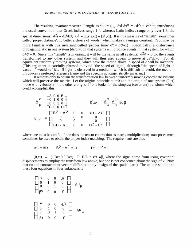
The resulting invariant measure "length" is d2σ = gµν dxµdxν = - d2s + c2d2t , introducingthe usual convention that Greek indices range 1-4, whereas Latin indices range only over 1-3, the

spatial dimensions: d2s = dxidxj; xµ = (x,y,z,ct) = (xi ,ct). It is this measure of "length", sometimescalled 'proper distance', no better a choice of words, which makes c a unique constant. (You may bemore familiar with this invariant called 'proper time' dτ = dσ/c.) Specifically, a disturbancepropagating at c in one system (ds/dt=c in that system) will produce events in that system for whichd2σ = 0. Since this "length" is invariant, it will be the same in all systems: d2σ = 0 for the eventstransformed to any other system, and they will thus also appear to move at ds'/dt'=c. For allequivalent uniformly moving systems, which have the metric above, a speed of c will be invariant.(This argument is carefully phrased to avoid "the speed of light", although "the speed of light invacuum" would suffice. If light is observed in a medium, which is difficult to avoid, the mediumintroduces a preferred reference frame and the speed is no longer strictly invariant.)

It remains only to obtain the transformation law between uniformly moving coordinate systemswhich will preserve the metric. Let the origins coincide at t=0 and the origin of one system (0,ct)move with velocity v in the other along x. If one looks for the simplest (covariant) transform whichcould accomplish this

Λ αµ =

A 0 0 B

0 1 0 00 0 1 0C 0 0 D

g'µν = Λαµ Λ

βν gαβ

g'µν =

Β2 − Α 2 0 0 BD - AC

0 -1 0 00 0 -1 0

BD - AC 0 0 D2 - C2

where one must be careful if one does the tensor contraction as matrix multiplication; transposes mustsometimes be used to obtain the proper index matching. The requirements are thus

AC = BD Β2 − Α2 = -1 D2 - C2 = 1

(0,ct) → (- Bct,0,0,Dct) ⇒ B/D = v/c ≡β, where the signs come from using covariantdisplacements to employ the transform law above, but one is not concerned about the sign of v. Notethat co and contravariant vectors differ, but only in sign of the spatial part.) The unique solution tothese four equations in four unknowns is

γ 0 0 βγ

0 1 0 00 0 1 0

βγ 0 0 γ

= Λαµ

γ 0 0 -βγ

0 1 0 00 0 1 0

-βγ 0 0 γ

= Λαµ


12

γ ≡ 1

√1-β2

which give the rules for transforming tensors between uniformly moving systems.(Note that the metric is not positive definite here. The notion of physical vectors introduced in

Section III cannot be employed to disguise a difference between co and contravariant. An attempt todo so introduces √(-1), the origin of the ubiquitous i's which permeate non-tensor treatments of specialrelativity. It is ironic that the attempt to "hide" the metric by introducing "physical" vectors shouldresult in the rather unphysical appearance of imaginary dimensions.)

Because the metric does not depend upon position, we have the useful generalization, already

employed above, that not only is the displacement, dxµ, a contravariant vector, as it always must be,

but the coordinates or vector position of a point, xµ, is also a vector, which is not truein general and constitutes a major conceptual subtlety in tensor calculus. This is a great simplificationfor special relativity, and it means that the law above for transformation of contravariant vectors isalso the law for coordinate transformations.

Finally, note that gµν = gµν, which can be confirmed by direct calculation. (As noted earlier,the two must be matrix inverses of one another.)

All the usual relativistic effects follow in a straightforward manner from these equations. An

event at xo, cto occurs at γ (xo- βcto ), γ(cto - βxo) in the moving system. The origin of the initialcoordinates appears to be moving at -v in the new system, whereas the origin in the new systemappears to be moving at v in the initial system. Events at the point xo but separated by ∆to occur at

different points and different times, the time difference being γ ∆to, the well-known time dilation. Astationary bar with ends 0,cto and L,ct1 appears at

−βγcto , γ cto and γ (L-βct1 ),γ(ct1- βL)

Expressed in terms of a new t', t' =γ to and t' = γ(t1- βL/c)

−βct' , ct' and (L/γ) -βct', ct'

which implies that the ends appear separated by a distance L/γ, the contraction of length, if they areobserved (measured) simultaneously in the new system. The velocity addition formula follows simplyby applying two successive transformations:

(1+ββ')γγ' 0 0 -(β+β')γγ'

0 1 0 00 0 1 0

-(β+β')γγ' 0 0 (1+ββ')γγ'

=

γ" 0 0 -β"γ"

0 1 0 00 0 1 0

-β"γ" 0 0 γ"

β" ≡ β+β'

1+ββ'γ" = (1 + ββ')γγ' = γ"(β")

but note that the addition of two velocities in different directions gives much more complicated results;the transformations do not even commute.

If the physical laws are expressed in terms of relativistic vectors and tensors, they willtransform properly with coordinate system and have the same form in any system, as desired. Theanalog of velocity is

vµ ≡ dxµ/dτ dσ = cdτ


13

vµ = (γ vi,γc) pµ = mvµ =( pi, E/c)

These relations for the four-velocity follow directly if xi =vit, d2xi = v2d2t

d2τ = d2t - d2xi /c2 = (1-β2)d2t= d2t /γ2

This is a well-formed vector which reduces to the usual velocity for v << c; it is the only usefulrelativistic expression for velocity, and thus momentum. The fourth component of the momentumvector is identified as E because it becomes mc2 + (1/2)mv2 = K.E. + constant in the usual limit.

Because of the tensor transformation law, if p1µ =p2µ in one system, p'1µ =p'2µ in any other,and only momentum defined in this way will be conserved in all systems if it is conserved anysystem. Because the conserved momentum is that given by these expression, the relativistic equations

are often described as giving a mass increase γm, because pi = γmvi. The generalization of energy

is E = γ mc2. (Since only the rest mass ever appears, we shall omit mo and keep all factors of γexplicit.)

The equations of mechanics are

fµ ≡ dpµ

dτ = γ

dpµdt = γ(Fi,P/c) Fi=dpi/dt (Newtonian force) P =

dEdt

aµ ≡ dvµ

dτ = γ

dvµdt

Example: 'Uniform Acceleration'To illustrate the use of these equations, consider a particle subjected to a constant force, e.g. an

electron in a constant electric field, starting from rest. The spatial part of Newton's law, canceling γ's,

is simply dpidt = Fi =

d(γmvi)dt . For motion in one dimension, αo≡ F

mc, and d dt

β

√1-β2 = α o.

This may be integrated directly to give β(t) = αot

√1 + α o2t2

, which has the necessary v=at behavior

at small t and β ~ 1 at large t, and γ(t) = √1 + αo2t2 . This is a solution for the motion in a fixed

reference frame in which the particle was originally at rest. From the view of the particle, things aremore complicated, for the particle does not define an inertial frame. At best, one can consider asuccession of inertial frames in which the particle is instantaneously at rest. From the solution,

vµ = γ(v,0,0,c) and aµ = γc(αo,0,0, dγdt ) = γc(αo,0,0, βαo), the (contravariant) vector transform to

the particle 'rest' frame (at v) gives v'µ = (0,0,0,c), as it should, and a'µ = c(α o,0,0,0). Theconstant force in the laboratory frame implies a constant acceleration in the instantaneous rest frame;

the power, dEdt , is always zero in that frame because F.v = 0 there.


14

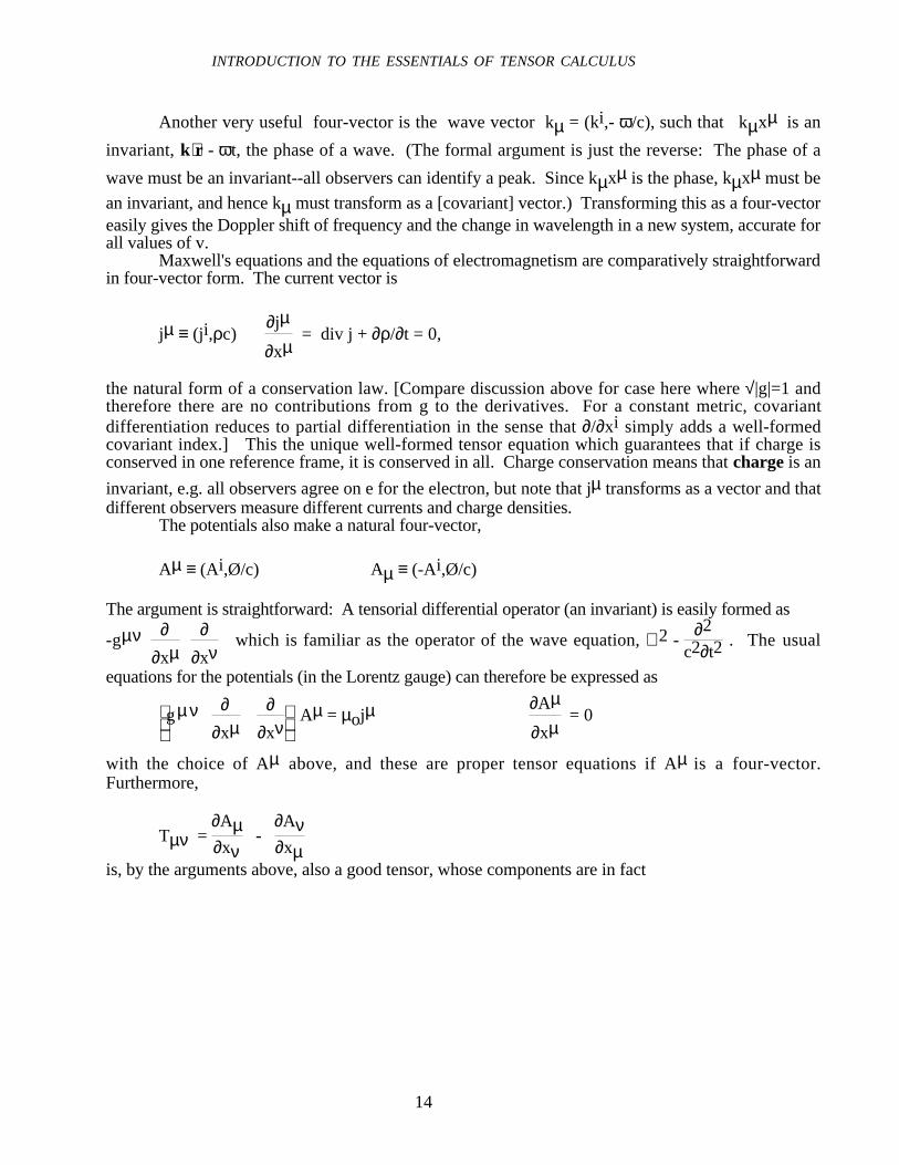
Another very useful four-vector is the wave vector kµ = (ki,- ω/c), such that kµxµ is an

invariant, k ⋅r - ωt, the phase of a wave. (The formal argument is just the reverse: The phase of a

wave must be an invariant--all observers can identify a peak. Since kµxµ is the phase, kµxµ must be

an invariant, and hence kµ must transform as a [covariant] vector.) Transforming this as a four-vectoreasily gives the Doppler shift of frequency and the change in wavelength in a new system, accurate forall values of v.

Maxwell's equations and the equations of electromagnetism are comparatively straightforwardin four-vector form. The current vector is

jµ ≡ (ji,ρc)∂jµ

∂xµ = div j + ∂ρ/∂t = 0,

the natural form of a conservation law. [Compare discussion above for case here where √|g|=1 andtherefore there are no contributions from g to the derivatives. For a constant metric, covariantdifferentiation reduces to partial differentiation in the sense that ∂/∂xi simply adds a well-formedcovariant index.] This the unique well-formed tensor equation which guarantees that if charge isconserved in one reference frame, it is conserved in all. Charge conservation means that charge is an

invariant, e.g. all observers agree on e for the electron, but note that jµ transforms as a vector and thatdifferent observers measure different currents and charge densities.

The potentials also make a natural four-vector,

Aµ ≡ (Ai,Ø/c) Aµ ≡ (-Ai,Ø/c)

The argument is straightforward: A tensorial differential operator (an invariant) is easily formed as

-gµν ∂

∂xµ

∂∂xν

which is familiar as the operator of the wave equation, ∇ 2 - ∂2

c2∂t2 . The usual

equations for the potentials (in the Lorentz gauge) can therefore be expressed as

gµν

∂∂xµ

∂

∂xν Aµ = µojµ

∂Aµ

∂xµ = 0

with the choice of Aµ above, and these are proper tensor equations if Aµ is a four-vector.Furthermore,

Tµν = ∂Aµ∂xν

- ∂Aν∂xµ

is, by the arguments above, also a good tensor, whose components are in fact


15

µ\ν

0 Βz −Βy Εx/c

-Βz 0 Βx Εy/c

Βy −Βx 0 Εz/c

−Εx/c −Εy/c −Εz/c 0

= Tµν

µ\ν

0 Βz −Βy −Εx/c

-Βz 0 Βx −Εy/c

Βy −Βx 0 −Εz/c

Εx/c Εy/c Εz/c 0

= Tµν

∂Tµν

∂xν = µo jµ

expresses the two Maxwell's equations with sources, Gauss and Ampere's Laws, directly. Since thefields are constructed from the potentials using the usual equations, the other two Maxwell's equationsare automatically satisfied, but they can also be expressed as

εαβγδ ∂Tβγ ∂xδ

= 0

noting that the simple permutation symbols are tensors when ||g||=1 (absolute value of the determinantof the metric tensor), a simple generalization of the arguments of Section II. One can construct twointeresting invariants from the fields as

Tµν Tνµ = |B|2 - |E/c|2 and εαβγδ Tαβ Tγδ = 2 E.B

These have important physical consequences, implying that if the field is purely electric in one frame,there will be a dominant electric field in all frames, and vise versa. Conversely, if there are bothelectric and magnetic fields in some frame, it is possible to find a frame in which one vanishes. Animportant consequence of the second invariant is that if the fields are transverse in one frame(perpendicular to one another), they will be so in all frames.

The Lorentz force expressions may also be constructed:

ƒν = Tµν jµ = -Tνµ jµ and fν = qTµν vµ = -qTνµ vµ

The covariant force density ƒν, appropriate to a continuous system with a current-density, charge-

density four-vector jµ, is to be distinguished from the four-vector force fν, which acts on a particle ofcharge q. These expressions are explicitly formed as invariant (tensor) expressions and may bedirectly computed to verify that they give the familiar results of electromagnetism (for the contravariantform):

ƒµ = ( ρEi + j x B, j .E/c) fµ = qγ(Ei + v x B, v.E/c)

The four-vector force fµ, which appears here has the same factor of γ multiplying the familiar terms asdid the corresponding four-vector in the tensor form of Newton's law.


16

These constructions of the tensor equivalents of mechanics and electromagnetism may appearto lack rigor, but that is not the case. If an equation is written as a proper equation among tensors,tensor calculus guarantees that it will remain true in all coordinate systems. Therefore an equation ofthe proper form which is correct in one coordinate system will be universal. You may find moredetailed arguments helpful in understanding relativistic effects, but they are not necessary. For

example, to prove that jµ is a four-vector, it is not necessary to examine current densities and chargedensities in one coordinate system and determine their complex transformations as velocities andvolumes transform between systems. It suffices to declare that charge conservation is a physical law.

Only ∂jµ

∂xµ = 0 with jµ = (ji,ρc) being a genuine four-vector is a proper tensor equation which

provides the usual form of the charge conservation equation in a reference system. Therefore jµ mustbe a four-vector. (It is a symptom of the Lorentz invariance of electromagnetism that the equation ofcharge conservation indeed has the familiar form in all inertial coordinate systems. However, the

tensor equations for mechanics involving fµ etc. include factors of γ and reduce to the familiar forms

only for low velocity, γ~ 1.)The most important application of this argument is to the electromagnetic field, the tensor and

transformation character of which would otherwise require considerable, tedious argument. Theargument above shows that the fields are thoroughly linked, being components of a single tensor.Since E and B are conventionally vectors, one might have expected analogous four-vectors, but thatwould create a conceptual difficulty in expressing a four-vector force coupling four-vector fields andthe four-vector velocity, a difficulty which is obviated by the tensor force expressions above. Thefield tensor transforms normally; for reference, the result is shown here:

µ\ν

0 γ(Βz - βΕy/c) -γ(Βy + βΕz/c) Εx/c

-γ(Βz - βΕy/c) 0 Βx γ(-βΒz + Εy/c)

γ(Βy + βΕz/c) -Βx 0 γ(βΒy + Εz/c)

−Εx/c -γ(-βΒz + Εy/c) -γ(βΒy + Εz/c) 0

= Tµν

The familiar vxB contribution to the new E is present, but there are factors of γ and contributions to Bas well.

The tensor form of energy conservation may be obtained by similar arguments, or it can beobtained as follows using methods analogous to those of the classical argument. (Since momentum-energy conservation already involves tensors, the four-vector analog is not particularly easy toconstruct.)

ƒν = Tµν jµ = 1

µo Tµν

∂Tµα

∂xα

= 1

2µo Tµν

∂Tµα

∂xα +

1

2µo

∂(Tµν Tµα)

∂xα - Tµα

∂Tµν

∂xα


17

Since ∂Tµν

∂xα +

∂T α µ

∂xν +

∂T να

∂xµ = 0 (if the indices are distinct, this is one of Maxwell's

equations εαβγδ ∂Tβγ ∂xδ

= 0, otherwise is it true by the antisymmetry of T),

ƒν = 1

2µo Tµν

∂Tµα

∂xα +

1

2µo

∂(Tµν Tµα)

∂xα + Tµ α

∂Tαµ

∂xν +

∂Tνα

∂xµ

= 1

2µo Tµν

∂Tµα

∂xα +

1

2µo

∂(Tµν Tµα)

∂xα +

12

∂(Tµα Tαµ )

∂xν +Tµα

∂Tνα

∂xµ

= 1

2µo Tµν

∂Tµα

∂xα +

1

2µo

∂(Tµν Tµα)

∂xα +

12

∂(Tµα Tαµ )

∂xν +

∂(Tµα Tνα )

∂xµ - Tνα

∂Tµα

∂xµ

By changing dummy indices and using the antisymmetry of T, the first and last terms cancel, and thesecond and fourth terms are identical, leaving

ƒν = 1

µo

∂(Tµν Tµα)

∂xα -

14

∂(Tµα Tµα )

∂xν =

∂Gµν

∂xµ

Gµν

= 1

µo

Tαν Tαµ - 14 (Tαβ Tαβ ) δ

µν

for the relativistic stress tensor. It can be converted to other forms, for example:

Gµν = 1

µo

gαβ Tβν Tαµ - 14 (Tαβ Tαβ) gµν

which is clearly symmetric, but the elements remain complicated functions of the fields. Thiscompletes the fundamental formulation of mechanics and electrodynamics in relativistic form.

VI. Covariant DifferentiationDifferentiation of tensors is not simple. The partial derivatives of an invariant form a good

(covariant) vector, and certain antisymmetric forms have been shown above to be tensors, butgenerally speaking, the partial derivatives of vectors (and perforce tensors) introduce derivatives of thetransform law and metric. Only for constant gij , e.g. Cartesian coordinates and special relativity, butnot even cylindrical or spherical coordinates, do partial derivatives produce tensors. The formulationof derivatives (i.e. finding definitions for derivatives of a tensor --- absolute and covariantdifferentiation) which do behave properly is subtle. Several approaches are possible; the one here is'geometric' rather than formal and strives to provide a basis for and understanding of the complicationswhich arise. Nevertheless, not all steps can be well motivated, and certain choices will become clearonly in retrospect.

Since only derivatives of invariants have tensor character, we begin by considering a simple,fundamental object, the tangent to a curve qi(u):


18

pi ≡ dqidu (1)

This is a well-formed contravariant vector, from which an invariant w = gijpipj may be constructed.Its derivative must likewise be an invariant

dwdu = 2 gijpi

dpjdu +

∂gij∂qk

pipjpk (2)

which can be written in this simple, symmetric form because of the definition of pi above. Afundamental (and rather obvious) theorem of tensor calculus, sometimes called the quotient rule,implies that if AiBi = Ø (an invariant) and Bi is an arbitrary contravariant vector, then Ai must be acovariant vector. One can thus factor out a term pi from this expression and conclude that theremainder is a good covariant vector. However, i is a dummy index; any of the three p factors in thefinal product could be extracted. In fact, a particular combination is particularly useful: the sum of thetwo symmetric forms in ij, minus the form using k:

fi = gij dpjdu + [jk,i] pjpk [ij,k] ≡

12

∂gjk∂qi

+ ∂gi k

∂qj -

∂gi j∂qk

(3)

where the bracket defines a famous object, the Christoffel symbol of the first kind. It is clear that this

fi is not the only covariant vector involving dpjdu, but the special symmetry of the Christoffel symbol

makes it an advantageous choice. There is an obvious corresponding contravariant vector

fi = dpidu + { }ijk pjpk { }ijk ≡ gil [jk,l] (4)

which employs the Christoffel symbol of the second kind. These objects are not tensors, theirtransformation law remaining to be inferred from the known transformation character of the otherterms in the equation, but raised and lowered indices are used to indicate the indices with which theyare to be summed in the usual convention.

This leads one to define a derivative, the absolute derivative, of pi as the contravariant vector

δpi

δu =

dpidu + { }ijk pjpk (5)

The significance of the Christoffel symbols may be understood as follows: If u is chosen to be length

s, then a 'straight line' would have a constant tangent δpi

δs = 0 as an invariant property. In Cartesian

coordinates, that is equivalent to dpids = 0, but this definition implies otherwise if the Christoffel

symbols are non-zero. In fact, in 'curved' coordinates, even ones as simple as cylindrical or spherical

systems, dpids ≠ 0 for a straight line, and a constant tangent vector has varying r,θ components along

the line in general. The Christoffel symbols embody this curvature and introduce it into the equations,

guaranteeing that only the proper dpids will produce

δpi

δs = 0. (Very similar equations and calculations

to those here appear in the rigorous generalization of a straight line, which is a geodesic, a curve ofvariationally stationary length or simply the 'shortest distance' if the metric is positive definite.)

As mentioned above, the transformation laws for Christoffel symbols may be adduced from thetensorial form of the terms in (3) and (4). Specifically from (4),


19

f'i = d2qi

d2u + { }ijk '

dqjdu

dqkdu

= ∂qi

∂xj

d2xj

d2u + { }j

lm dxldu

dxmdu (6)

∂qi

∂xj

d2xj

d2u =

∂qi

∂xj ddu

∂xj

∂ql dqldu =

∂qi

∂xj ∂xj

∂ql d2ql

d2u +

∂qi

∂xj ∂2xj

∂ql∂qp dqldu

dqpdu

= d2qi

d2u +

∂qi

∂xt ∂2xt

∂qj∂qk dqjdu

dqkdu

The second derivatives of qi match, leaving

{ }ijk ' dqjdu

dqkdu

= ∂qi

∂xt ∂2xt

∂qj∂qk dqjdu

dqkdu +

∂qi

∂xt { }tlm

∂xl

∂qj ∂xm

∂qk dqjdu

dqkdu

{ }ijk ' = ∂qi

∂xn ∂2xn

∂qj∂qk + { }nlm

∂xl

∂qj ∂xm

∂qk ∂qi

∂xn (7)

This implies that the Christoffel symbols transform like tensors, but with an additional term, whichinvolves the second derivatives of the coordinate transformations. They therefore remain zero for alllinear transformations like rotation and the Lorentz group. They are non-zero in cylindrical andspherical coordinates, and the transformation law (7) from Cartesian can be as convenient forcalculation as the definition (4). The same procedure may be applied to (3) to give

[ij,k] ' = glm ∂xl

∂qi ∂2xm

∂qj∂qk + [lm,n] ∂xl

∂qi ∂xm

∂qj ∂xn

∂qk (8)

An absolute derivative was defined for the contravariant vector pi ≡ dqidu, but the calculation

depended on the special properties of p. However, a straightforward generalization is possible, basedon the invariant Ø = gijpiTj, for any vector field Tj defined along the curve qj(u):

dØdu = gij

dpidu Tj + gij pi

dTjdu +

∂gij∂qk

piTjpk

using (3),

= (fj - [ik,j] pipk)Tj + gij pi dTjdu +

∂gij∂qk

piTjpk

dØdu - fjTj = gij pi

dTjdu + [jk,i] piTjpk (9)

Since the quantity on the left in an invariant, so is the right, and factoring out pi implies that

gij dTjdu + [jk,i] Tjpk = fi

a covariant vector. The corresponding contravariant vector is the appropriate absolute derivative:

δTi

δu ≡

dTidu + { }ijk Tj dqk

du (10)


20

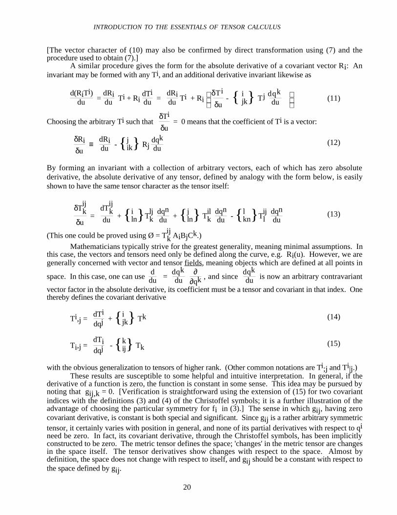
[The vector character of (10) may also be confirmed by direct transformation using (7) and theprocedure used to obtain (7).]

A similar procedure gives the form for the absolute derivative of a covariant vector Ri: Aninvariant may be formed with any Ti, and an additional derivative invariant likewise as

d(RiTi)du =

dRidu Ti + Ri

dTidu =

dRidu Ti + Ri

δTi

δu - { }ijk Tj dqk

du (11)

Choosing the arbitrary Ti such that δTi

δu = 0 means that the coefficient of Ti is a vector:

δRiδu

≡ dRidu - { }jik Rj

dqkdu

(12)

By forming an invariant with a collection of arbitrary vectors, each of which has zero absolutederivative, the absolute derivative of any tensor, defined by analogy with the form below, is easilyshown to have the same tensor character as the tensor itself:

δT

ijk

δu =

dTijk

du + { }iln Tljk

dqndu

+ { }jln Tilk

dqndu

- { }lkn T

ijl

dqndu

(13)

(This one could be proved using Ø = Tijk AiBjCk.)

Mathematicians typically strive for the greatest generality, meaning minimal assumptions. Inthis case, the vectors and tensors need only be defined along the curve, e.g. Ri(u). However, we aregenerally concerned with vector and tensor fields, meaning objects which are defined at all points in

space. In this case, one can use ddu =

dqkdu

∂∂qk , and since

dqkdu is now an arbitrary contravariant

vector factor in the absolute derivative, its coefficient must be a tensor and covariant in that index. Onethereby defines the covariant derivative

Ti,j = dTi

dqj + { }ijk Tk (14)

Ti,j = dTidqj - { }kij Tk (15)

with the obvious generalization to tensors of higher rank. (Other common notations are Ti;j and Ti|j.)These results are susceptible to some helpful and intuitive interpretation. In general, if the

derivative of a function is zero, the function is constant in some sense. This idea may be pursued bynoting that gij,k = 0. [Verification is straightforward using the extension of (15) for two covariantindices with the definitions (3) and (4) of the Christoffel symbols; it is a further illustration of theadvantage of choosing the particular symmetry for fi in (3).] The sense in which gij , having zerocovariant derivative, is constant is both special and significant. Since gij is a rather arbitrary symmetrictensor, it certainly varies with position in general, and none of its partial derivatives with respect to qineed be zero. In fact, its covariant derivative, through the Christoffel symbols, has been implicitlyconstructed to be zero. The metric tensor defines the space; 'changes' in the metric tensor are changesin the space itself. The tensor derivatives show changes with respect to the space. Almost bydefinition, the space does not change with respect to itself, and gij should be a constant with respect tothe space defined by gij .


21

The concept of 'constancy' may be developed by noting that (11) may be written as

d(RiTi)du = Ri

δTi

δu +

δRiδu

Ti (16)

Applying this to a single vector, if δTi

δu = 0, then the length of Ti remains constant along u.

Furthermore, the angle between two vectors may be defined in the usual sense as RiTi = |Ri||Ti|cos θ,

|Ti| = √TiTi . If both vectors have zero absolute derivative along u, then their lengths and the angle

between them remain constant. For this reason, if δTi

δu = 0, the vector Ti is considered to be

propagated parallel to itself along u. Parallelism is easily defined at a point in the usual sense that RiTi

= ± |Ri||Ti|, but vectors at different points cannot generally be compared. This offers a generalizationwhich preserves most of the usual properties. [Unfortunately, uniqueness is not one of them; differentcurves u between a pair of points (A, B) may lead to different Ti at B starting from a given Ti at A.]

An interpretation of Christoffel symbols can again be given from noting their role in a δTi

δu = 0

condition as that of driving dTidu, causing Ti to change to compensate for the 'curvature' of the space.

VII. Geodesics and LagrangiansAs noted above, the concepts of parallelism, straight line, and really all non-local (global)

comparisons require some specialization in general metric space. They cannot be carried over with all

their familiar properties. A primitive (if 'correct') notion of straight line as δpi

δs = 0 (pi =

dqids ) was

introduced in the previous section in interpreting the meaning of absolute differentiation, but a moregeneral formulation is useful. The fundamental formulation is based on a variational principle, andsuch principles are also important for mechanics.

To review, if a definite integral I , whose value is expressed as a functional of functions of aparameter u between fixed end points, is to have an extremum (maximum, minimum, or possibly aninflection point),

δI = δ

⌡⌠

u1

u2

L(dqidu,qi(u),u) du = 0 (1)

By the usual argument in calculus of variations, if the set of functions qio(u) is a solution, then for a

small variation about that, qi = qio + δqi, δI must be second order in δqi, and the first order variation

is zero. (This is simply a generalization of the fact that the first derivative of a function is zero atextrema.) If L is then regarded as a function of the functions listed above regarded as independent,

δI = ∫u1

u2du

∂ L

∂q'i d(δqi)

du + ∂ L ∂qi

δqi = 0 where q'i =dqidu (2)

and a sum over the index i is understood. The first term may be integrated by parts, and if the endpoints are prescribed so that δqi(u1) = δqi(u2) = 0, the condition may be written as


22

∫u1

u2du

ddu

∂ L

∂q'i -

∂ L ∂qi

δqi = 0 (3)

since the δqi are arbitrary, the integral will be zero only if all its coefficients zero, which are the well-known Euler-Lagrange equations for the variational problem.

ddu

∂ L

∂q'i -

∂L ∂qi

= 0 (4)

The application to straight lines arises because a straight line is, among other things, theshortest distance between two points, and this criterion can be formulated in any metric space. Ageodesic is defined as a curve for which

δI = δ

⌡⌠

u1

u2

√

gij

dqidu

dqjdu du = 0 (5)

and in cases like special relativity for which the metric is not positive definite and there are curves ofzero length, the integral may be a maximum. In any case, the solutions qi(u) are geodesics and thebest generalization of a "straight line" in a general metric space. The Euler equations are thus

ddu

∂√ w

∂q'i -

∂√ w∂qi

= 0 = ddu

1

√ w

∂ w ∂q'i

- 1

√ w ∂w ∂qi

for w = gij dqidu

dqjdu

and if u is chosen to be the measure of distance ds2 = gij dqidu

dqjdu du2, w = 1 and

dwds = 0 leaving

dds

∂ w

∂q'i -

∂w ∂qi

= 0 = dds

2gij

dqjds -

∂gjk∂qi

dqjds

dqkds (6)

as the equation of the geodesic. Computing the derivative through the qi dependence and rearrangingdummy indices produces

2gij d2qj

ds2 +

∂gij∂qk

dqjds

dqkds +

∂gik∂qj

dqjds

dqkds -

∂gjk∂qi

dqjds

dqkds = 0 (7)

which, through no accident, can be written

gij d2qj

ds2 + [jk,i]

dqjds

dqkds = 0 or

d2qi

ds2 +{ }ijk dqj

ds dqkds = 0 (8)

which are the standard forms for these equations.Variational principles are also used to form the Lagrangian and related equations of motion.

The familiar results may be extended to construct relativistically proper forms, but somewhatindirectly. The normal construction of L = T-V with ∫dt has no clear tensor equivalent. Instead, we

must try to find an invariant L such that ∫Ldu generates the correct equations of motion. For example,


23

L = mc √gαβ dxαdu

dxβdu (9)

is manifestly invariant and also independent of position (only derivatives enter) and thus a possiblestarting point as the Lagrangian for a free particle. The Euler equations are

mc d du

gαβ

dxβdu

√gαβ dxαdu

dxβdu

= 0 (10)

If u is now chosen to be the invariant parameter τ, the radical becomes the invariant constant c, and theequations reduce to the standard equation of motion for a free particle:

m d2xα

dτ2 = 0 =

dpα

dτ (11)

With this start, the Lagrangian for a particle in an electromagnetic field could be

L = mc √gαβ dxαdu

dxβdu + q gαβ

dxαdu Aβ (12)

which is again an invariant and linear in q, vµ, and Aβ; one can argue the second term as the onlyplausible one. The equations of motion thereby implied are

d du

mc gαβ

dxβdu

√gαβ dxαdu

dxβdu

+ q gαβ Aβ - q gµβ dxµdu

∂Aβ

∂xα = 0 (13)

and with the same choice of u as τ and extraction of the τ dependence of Aβ through the xµ,

gαβ m d2xβ

dτ2 = q

dxµ

dτ

gµβ ∂Aβ

∂xα - gαβ

∂A β

∂xµ = q

dxµ

dτ

∂Aµ

∂xα -

∂A α∂xµ

= q dxµ

dτ Tµα = fα (14)

the same equation as obtained previously, thus confirming the choice of L above.The procedures of classical mechanics may be continued to construct a Hamiltonian from the

conjugate momenta


24

Pα = ∂L

∂

dxα

du

= mc gαβ

dxβdu

√gαβ dxαdu

dxβdu

+ q gαβ Aβ i.e., Pµ = mvµ + q Aµ (15)

(The partials of L are always taken with respect to a contravariant quantity and generate a covariantindex in consistent analogy with the usual tensor derivatives with respect to coordinates, the dqi beingcontravariant, although no real tensor character can be ascribed to the partial derivatives associated withthe derivation of the Euler-Lagrange equations.)

The Hamiltonian is then

H = 12 ( )Pα vα - L where mvµ = Pµ - q Aµ (16)

is to be used to eliminate vµ in favor of Pµ. Straightforward algebra produces the Hamiltonian as

H = gαβ2m ( Pα - q Aα) ( Pβ - q Aβ) -

mc2

2 (17)

and the Hamiltonian equations of motion:

dxαdτ

= ∂H

∂Pα =

gαβm ( Pβ - q Aβ) or

dxα

dτ =

Pα - q Aαm (18)

dPµdτ

= - ∂H

∂xµ =

qgαβm ( Pα - q Aα)

∂Aβ

∂xµ(19)

The first is the trivial dxα

dτ = vµ, and the second, after elimination of P from (15) on both sides,

leaves the same equation of motion as that obtained above from the Lagrangian (14), because dAµ

dτexpands into the remaining portion of the E-M coupling term.

________________________________________________________________________

introduction to the essentials of tensor calculusphy315/tensors.pdf · introduction to the...

Documents