introduction to the physics of free electron laser and...

1

Introduction to the Physics of Free Electron Laser and Comparison

with Conventional Laser Sources

G. Dattoli1, M. Del Franco1, M. Labat1, P. L. Ottaviani2 and S. Pagnutti3 1ENEA, Sezione FISMAT, Centro Ricerche Frascati, Rome

2INFN Sezione di Bologna 3ENEA, Sezione FISMET, Centro Ricerche Bologna

Italy

1. Introduction

The Free Electron Laser (FEL) can be considered a laser, even though the underlying

emission process does not occur in an atomic or a molecular system, with population

inversion, but in a relativistic electron beam, passing through the magnetic field of an

undulator. Several parameters (such as gain, saturation intensity, etc.) are common to both

devices and this allows a unified description. The origin of Laser traces back to the

beginning of the last century, when Planck derived the spectral distribution of the radiation

from a "blackbody" source, a device absorbing all the incident radiation and emitting with a

spectrum which only depends on its temperature. A perfectly reflective cavity, with a little

hole, can be considered a blackbody source; the radiated energy results from the standing

wave or resonant modes of this cavity. The Planck distribution law, yielding the equilibrium

between a radiation at a given frequency and matter at a given temperature T, is the

following:

3

2 2 exp 1

I d d

ckT

(1)

h, 2 ,

2frequency .

( )I d is the energy per unit surface, per unit time, emitted in the frequency interval

d . Its fundamental nature can be stressed by noting that it crucially depends on

three constants h, k and c the Planck, the Boltzmann constants and the light velocity,

respectively. Its derivation required the assumption that the changes in energy are not

continuous, but discrete. The Plank theory prompted Bohr to make a further use of the

discretization (or better quantization) concept to explain the atom stability. He assumed that

the electrons, in an atomic system, are constrained on a stationary orbit, whose energetic

www.intechopen.com

Free Electron Lasers

2

level is fixed and can only exchange quanta of radiation with the external environment. This

point of view allowed Einstein to formulate the theory of spontaneous and stimulated

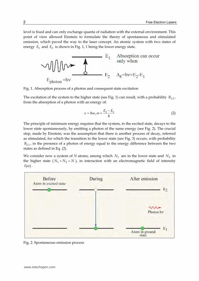
emission, which paved the way to the laser concept. An atomic system with two states of

energy 1E and 2E is shown in Fig. 1, 1 being the lower energy state.

Fig. 1. Absorption process of a photon and consequent state excitation

The excitation of the system to the higher state (see Fig. 1) can result, with a probability 1 2B ,

from the absorption of a photon with an energy of:

2 1,E E

(2)

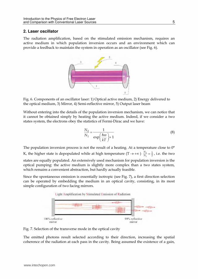
The principle of minimum energy requires that the system, in the excited state, decays to the

lower state spontaneously, by emitting a photon of the same energy (see Fig. 2). The crucial

step, made by Einstein, was the assumption that there is another process of decay, referred

as stimulated, for which the transition to the lower state (see Fig. 3) occurs, with probability

2 1B , in the presence of a photon of energy equal to the energy difference between the two

states as defined in Eq. (2).

We consider now a system of N atoms, among which 1N are in the lower state and 2N in

the higher state ( 1 2N N N ), in interaction with an electromagnetic field of intensity

( )I .

Fig. 2. Spontaneous emission process

www.intechopen.com

Introduction to the Physics of Free Electron Laser and Comparison with Conventional Laser Sources

3

Fig. 3. Stimulated emission process

The equilibrium condition of the atomic system with the radiation is therefore given by:

1 1 2 2 2 1 2 2 1( ) ( )N B I N B I N A (3)

where 2 1A represents the spontaneous emission contribution, independent of ( )I . In the

conditions of thermodynamic equilibrium at temperature T, the number of atoms per unit

volume in a given state of energy iE is described by the Boltzmann distribution law:

iiE KTiN e . From this relation, one can derive the ratio 1

2

N

N in terms of energy difference

and absolute temperature, namely 1

2

expN

N kT

, which combining with Eq. (3), yields:

2 1

1 2 2 1

( )( )h

kT

AI

B exp B

(4)

Assuming that the absorption and stimulated emission processes are perfectly symmetric,

i.e. that m n n mB B , and using the Wien law, the spontaneous emission can be written as:

3

, ,2 2n m m nA Bc

(5)

Eq. (4) provides therefore the Planck distribution law. The importance of this result stems from the fact the Planck distribution has been derived on the basis of an equilibrium condition and on the new concepts of spontaneous and stimulated emission. The main difference between the two processes is that, in the case of the spontaneous emission, the atoms decay randomly in time and space, generating photons uncorrelated in phase and direction; in the other, the atoms decay at the same time, generating “coherent” photons, with phases and directions corresponding to those of the incident photon. Given a certain number of atoms, all (or most of them) in the higher level, one can get a substantive amplification process from one single photon (see Fig. 4).

www.intechopen.com


4

Fig. 4. Stimulated emission

We consider a medium of 1 2N N N systems of two states, in interaction with an

electromagnetic field with the energy of a single photon 2 1E E . During the

propagation in the z direction (see Fig. 5), the variation of the number of photons n of the

field is driven by a differential equation deriving from Eq. (3):

2 1 1 2 2 1 2( )dn

N N b n a Ndz

(6)

Fig. 5. Increment of the radiation

The coefficients of emission and absorption have been redefined to take into account the physical dimensions. The solution of Eq. (6) is:

0

( ) 1( ) ( )

exp zn z n exp z

, 2 1 2 1 1 2 2( )N N b a N (7)

where 0n is the initial number of photons of the field. Eq. (7) consists of two parts, and one

(the spontaneous emission term) is independent of the initial number of photons. We

consider the case in which the spontaneous emission contribution can be neglected. If

2 1N N , i.e. if there are less atoms in the excited than in the ground state, then 0 and

Eq. (7) becomes: 0( ) ( )n z n exp z , corresponding to the Beer-Lambert law of absorption

and the coefficient can be interpreted as a coefficient of linear absorption. When 2 1N N ,

the number of photons remains constant. The amplification is possible if 2 1N N , i.e. when

a population inversion has occurred (namely the system has been brought to the “excited”

state through some mechanism). In this case, the coefficient is understood as the small

signal gain coefficient. The amplification can be seen as a chain reaction: a photon causes the

decay of the excited state, creating a "clone", and, following the same process, both lead to

the "cloning" of other two photons, and so on. Adding the spontaneous emission, the chain

can be started without the need of an external field.

These few introductory remarks provide the elements of the light amplification, we will see how it can be implemented to realize a laser oscillator.

www.intechopen.com


5

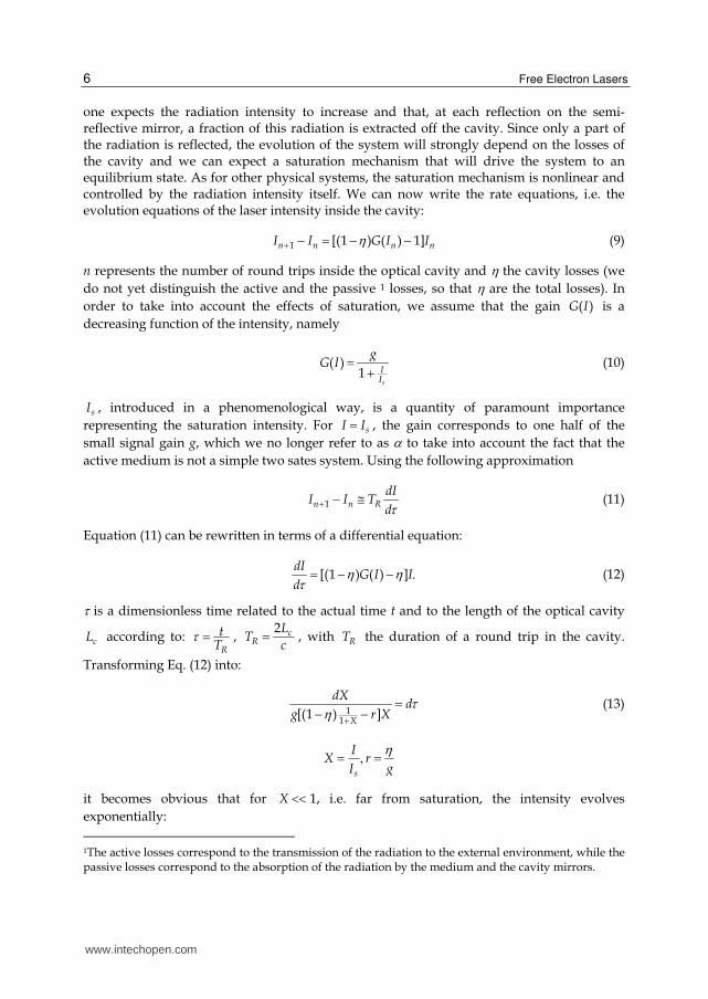
2. Laser oscillator

The radiation amplification, based on the stimulated emission mechanism, requires an active medium in which population inversion occurs and an environment which can provide a feedback to maintain the system in operation as an oscillator (see Fig. 6).

Fig. 6. Components of an oscillator laser: 1) Optical active medium, 2) Energy delivered to the optical medium, 3) Mirror, 4) Semi-reflective mirror, 5) Output laser beam

Without entering into the details of the population inversion mechanism, we can notice that it cannot be obtained simply by heating the active medium. Indeed, if we consider a two states system, the electrons obey the statistics of Fermi-Dirac and we have:

2

1

1

exp 1

N

N

kT

(8)

The population inversion process is not the result of a heating. At a temperature close to 0°

K, the higher state is depopulated while at high temperature (T ) 2

1

12

N

N , i.e. the two

states are equally populated. An extensively used mechanism for population inversion is the optical pumping: the active medium is slightly more complex than a two states system, which remains a convenient abstraction, but hardly actually feasible.

Since the spontaneous emission is essentially isotropic (see Fig. 7), a first direction selection can be operated by embedding the medium in an optical cavity, consisting, in its most simple configuration of two facing mirrors.

Fig. 7. Selection of the transverse mode in the optical cavity

The emitted photons result selected according to their direction, increasing the spatial coherence of the radiation at each pass in the cavity. Being assumed the existence of a gain,

www.intechopen.com


6

one expects the radiation intensity to increase and that, at each reflection on the semi-reflective mirror, a fraction of this radiation is extracted off the cavity. Since only a part of the radiation is reflected, the evolution of the system will strongly depend on the losses of the cavity and we can expect a saturation mechanism that will drive the system to an equilibrium state. As for other physical systems, the saturation mechanism is nonlinear and controlled by the radiation intensity itself. We can now write the rate equations, i.e. the evolution equations of the laser intensity inside the cavity:

1 [(1 ) ( ) 1]n n n nI I G I I (9)

n represents the number of round trips inside the optical cavity and the cavity losses (we

do not yet distinguish the active and the passive 1 losses, so that are the total losses). In

order to take into account the effects of saturation, we assume that the gain ( )G I is a

decreasing function of the intensity, namely

( )1

s

II

gG I (10)

sI , introduced in a phenomenological way, is a quantity of paramount importance

representing the saturation intensity. For sI I , the gain corresponds to one half of the

small signal gain g, which we no longer refer to as to take into account the fact that the

active medium is not a simple two sates system. Using the following approximation

1n n R

dII I T

d (11)

Equation (11) can be rewritten in terms of a differential equation:

[(1 ) ( ) ]dI

G I Id

(12)

is a dimensionless time related to the actual time t and to the length of the optical cavity

cL according to: R

tT

, 2 c

R

LT

c, with RT the duration of a round trip in the cavity.

Transforming Eq. (12) into:

1

1[(1 ) ]

X

dXd

g r X

(13)

s

IX r

I g

it becomes obvious that for X 1, i.e. far from saturation, the intensity evolves

exponentially:

1The active losses correspond to the transmission of the radiation to the external environment, while the passive losses correspond to the absorption of the radiation by the medium and the cavity mirrors.

www.intechopen.com


7

0 ([(1 ) ] )X X exp g (14)

It is also obvious that the equilibrium ( dXd = 0) is reached when the intensity in the cavity is

such that ( )1

G I and therefore

1

[ 1]E sI g I

(15)

Since in most cases 1, the extracted power at equilibrium (assuming that the losses are

only active losses) is given by:

out E sI I gI (16)

This relation is an additional evidence of the importance of the saturation intensity, which along with the gain defines the power which can be extracted from the cavity. The evolution of the laser power inside the cavity as a function of the number of round trips is reported in Fig. 8.

Fig. 8. Laser intensity (arb. unit) vs round trip number for g=15% and h=2%

The intensity first increases exponentially and then slows because of the saturation mechanism. When the gain equals the losses, the system reaches a stationary state and the power can be extracted off the cavity.

Despite not mentioning it before, the population inversion requires a sufficient level of

power, which we refer to as pump, that will be further partially transformed into laser

power. The ratio between the extracted laser power and the pump power represents the

efficiency of the system.

We have seen that the optical cavity is an essential element of an oscillator, since it confines the electromagnetic radiation, selects the transverse and longitudinal modes, thus creating the spatial and temporal coherence of the radiation.

The radiation field inside the optical cavity, whose components have a small angle with respect to the cavity axis, is successively reflected by the mirrors. This enables to select the components travelling in a direction parallel to the cavity axis. The interfering of the waves in the cavity leads to the formation of stationary waves at given frequencies, depending on the distance between the mirrors. In the case of planar and parallel mirrors, separated by a

www.intechopen.com


8

distance L, the stationary condition for the wave frequencies is: 2c

n Ln , n being integer.

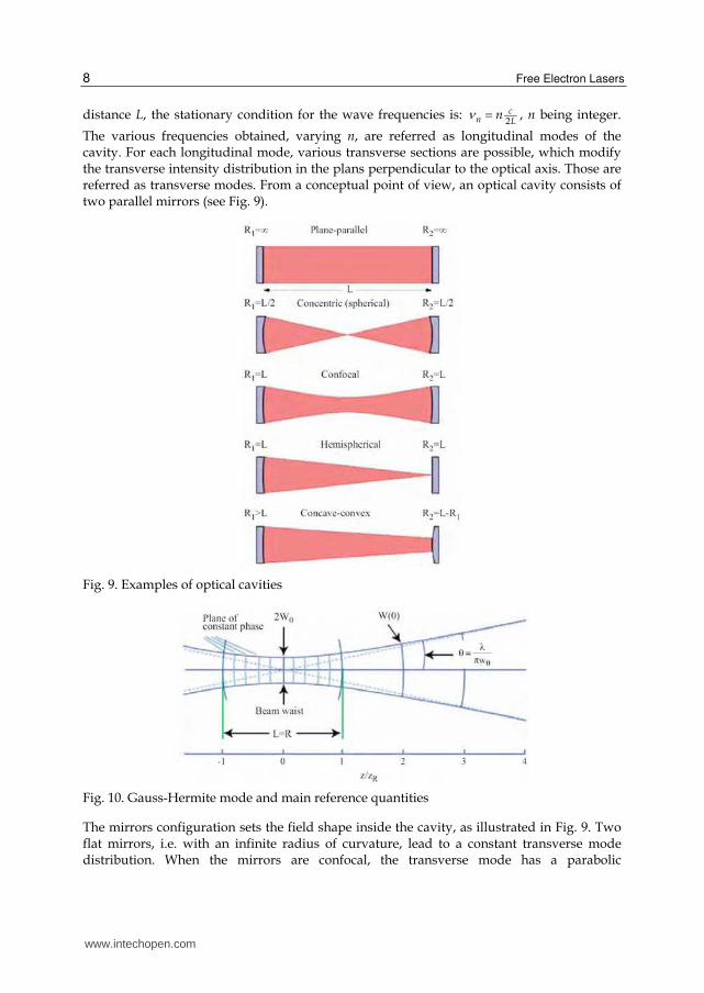
The various frequencies obtained, varying n, are referred as longitudinal modes of the cavity. For each longitudinal mode, various transverse sections are possible, which modify the transverse intensity distribution in the plans perpendicular to the optical axis. Those are referred as transverse modes. From a conceptual point of view, an optical cavity consists of two parallel mirrors (see Fig. 9).

Fig. 9. Examples of optical cavities

Fig. 10. Gauss-Hermite mode and main reference quantities

The mirrors configuration sets the field shape inside the cavity, as illustrated in Fig. 9. Two flat mirrors, i.e. with an infinite radius of curvature, lead to a constant transverse mode distribution. When the mirrors are confocal, the transverse mode has a parabolic

www.intechopen.com


9

longitudinal profile, which we will discuss more in details later. Additional configurations are shown in Fig. 9. In the case of a confocal cavity, the transverse modes are the Gauss-Hermite modes and, as previously mentioned, the longitudinal profile of the mode is parabolic (see Fig. 10).

The fundamental mode corresponds to a Gaussian distribution defined as:

222( )20

0( ) ( )( )

r

w zwI r z I e

w z

(17)

where r is the distance to the axis, w is the rms spot size of the transverse mode:

20( ) [1 ( ) ]

R

zw z w

z , 0

2

Lw

, 20

R

wz

(18)

0w is the beam waist, i.e. the minimum optical beam transverse dimension, Rz the Rayleigh

length, corresponding to the distance for which 0( ) 2w z w . For the fundamental mode,

2Rz L . The divergence of the mode is related to the former parameters according to:

20w

(19)

is referred as the angle of diffraction in the far field approximation.

The longitudinal modes are equally separated in frequency by f, which depends on the cavity length according to:

2c

fL

(20)

Fig. 11. Gain and loss spectra, longitudinal mode locations, and laser output for single mode laser operation

www.intechopen.com


10

The gain bandwidth of the active medium performs the mode selection and therefore allows the amplification of the modes within this bandwidth only. Those modes oscillate independently with random phase and beating. A longitudinal mode-locking enables to fix the longitudinal modes phases so that they all oscillate with one given phase [2]. It seems obvious that, in theory, varying the losses and therefore the gain profile would allow to suppress the competition in between modes and choose for instance the one with higher gain, as illustrated in Fig. 11.

But it’s also obvious that this is obtained to the detriment of the output laser power. We will now discuss alternative and less drastic methods to suppress the destructive mode competition using the previously mentioned mode-locking.

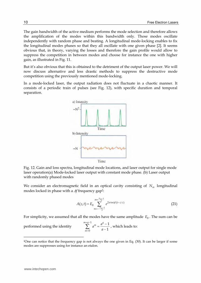
In a mode-locked laser, the output radiation does not fluctuate in a chaotic manner. It consists of a periodic train of pulses (see Fig. 12), with specific duration and temporal separation.

Fig. 12. Gain and loss spectra, longitudinal mode locations, and laser output for single mode laser operation(a) Mode-locked laser output with constant mode phase. (b) Laser output with randomly phased modes

We consider an electromagnetic field in an optical cavity consisting of mN longitudinal

modes locked in phase with a f frequency gap2:

1

2

1

2

2 ( )0( )

Nm

Nm

mim f t z c

m

A z t E e

(21)

For simplicity, we assumed that all the modes have the same amplitude 0E . The sum can be

performed using the identity 1

0

1

1

m q qm

m

aa

a

, which leads to:

2One can notice that the frequency gap is not always the one given in Eq. (30). It can be larger if some modes are suppresses using for instance an etalon.

www.intechopen.com


11

0

[ ( )]( )

[ ( )]msin N f t z c

A z t Esin f t z c

(22)

The intensity of the laser is defined as the squared moduleus of the former expression, which gives, at z =0:

2 20

[ ]( ) [ ]

[ ]msin N f t

I t Esin f t

(23)

The result of Eq. (23) is illustrated in Fig. 12. The radiation consists of a train of peaks,

separated by a distance 1 Tf

with a width 1N fm. The intensity of the peaks is

proportional to the square of the number of involved modes 2 20p mI N E , while the average

intensity is proportional to mN , i.e. 20M mI N E . Finally, it is important to notice that in the

case of random phases, the output laser intensity corresponds to the average intensity of the

mode-locked laser and that the fluctuations have a correlation time equal to the duration of

one single pulse of the mode-locked laser. Since the former remarks are of notable interest

for the laser applications and for further discussions, we provide with additional precisions

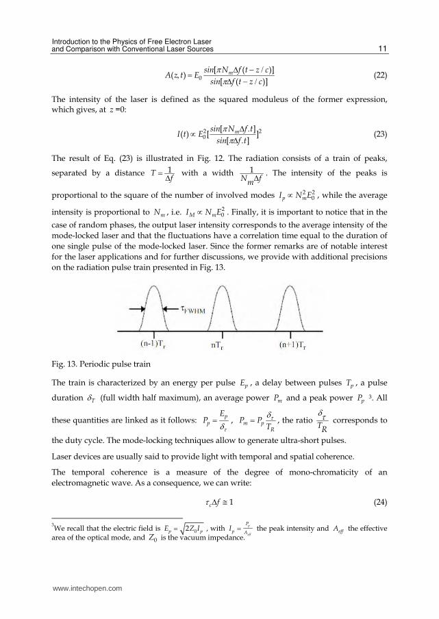
on the radiation pulse train presented in Fig. 13.

Fig. 13. Periodic pulse train

The train is characterized by an energy per pulse pE , a delay between pulses pT , a pulse

duration T (full width half maximum), an average power mP and a peak power pP 3. All

these quantities are linked as it follows: p

p

EP

, m pR

P PT , the ratio

TR

corresponds to

the duty cycle. The mode-locking techniques allow to generate ultra-short pulses.

Laser devices are usually said to provide light with temporal and spatial coherence.

The temporal coherence is a measure of the degree of mono-chromaticity of an

electromagnetic wave. As a consequence, we can write:

1c f (24)

3We recall that the electric field is 02p pE Z I , with p

eff

P

p AI the peak intensity and effA the effective

area of the optical mode, and 0Z is the vacuum impedance.

www.intechopen.com


12

In the case of a mode-locked laser, the coherence time is essentially given by the distance in

between the radiation packets. The coherence length cl can be calculated using Eq. (24):

2

( )c cl c (25)

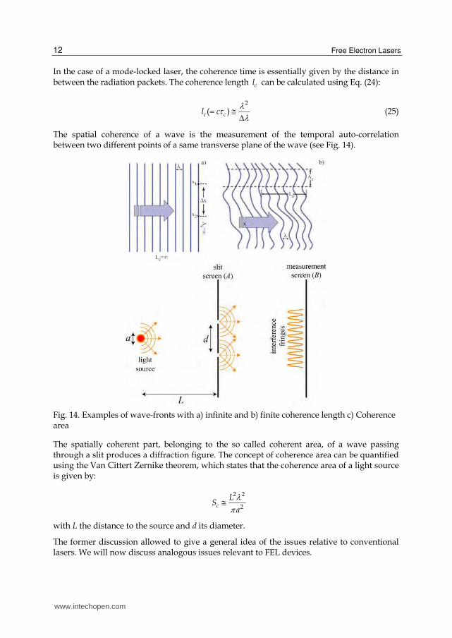
The spatial coherence of a wave is the measurement of the temporal auto-correlation between two different points of a same transverse plane of the wave (see Fig. 14).

Fig. 14. Examples of wave-fronts with a) infinite and b) finite coherence length c) Coherence area

The spatially coherent part, belonging to the so called coherent area, of a wave passing through a slit produces a diffraction figure. The concept of coherence area can be quantified using the Van Cittert Zernike theorem, which states that the coherence area of a light source is given by:

2 2

2c

LS

a

with L the distance to the source and d its diameter.

The former discussion allowed to give a general idea of the issues relative to conventional lasers. We will now discuss analogous issues relevant to FEL devices.

www.intechopen.com


13

3. The free electron laser

In this and in the forthcoming sections we will discuss laser devices operating with an active

medium, consisting of free relativistic electrons [3,5]. A few notions and a glossary of

relativistic kinematics are therefore necessary. The total energy E of a particle of mass m

moving with a velocity is given by:

2

02

1

1

vE m c

c (26)

is the reduced velocity and the relativistic factor. The total energy corresponds to the

sum of the kinetic and mass energy, the mass energy being given by 20m c . The factor is a

measure of the particle energy, and -1 of the kinetic energy. In addition: 2

11

In the high energy case 1, the reduced velocity becomes2

11

2

and the particle is said “ultra-relativistic”.

We now consider the main characteristics of the electrons: a charge e 1.610 19 C and a

mass em 0.51 MeV (1 MeV=10 6 eV, 1 eV=1.610 19 J). The adjective relativistic is used

when the kinetic energy of the electrons is of the order of a few MeV. Finally, a charged

particle beam is associated to a power equal to the product of its energy with its current:

( ) ( ) ( )P MW I A E MeV (27)

A 20 MeV beam with a current of 2 A has a power of 40 MW. Such power is delivered to the

beam by the accelerator. From now on, we will refer to LINAC accelerator, i.e. linear

accelerators, where the acceleration is performed in radiofrequency cavities. The electron

beam power corresponds in the case of free electron lasers, to the pump power in the case of

conventional lasers.

Free electrons passing through a magnetic field produces flashes of Bremsstrahlung

radiation. Synchrotron light sources rely on this process. We consider the case of a magnetic

field delivered by an undulator:

0

2(0 ( ) 0)

u

zB B sin

(28)

Such field is oscillating in the vertical direction with a peak value 0B and a periodicity u . It

can be obtained with two series of magnets with alternative N-S orientation, as illustrated in

Fig. 15.

The Lorentz force, due to the undulator field, introduces a transverse component in the

electron motion, initially exclusively longitudinal. The electron motion in the magnet is

governed by (Gaussian units):

www.intechopen.com


14

dp e

v Bdt c

(29)

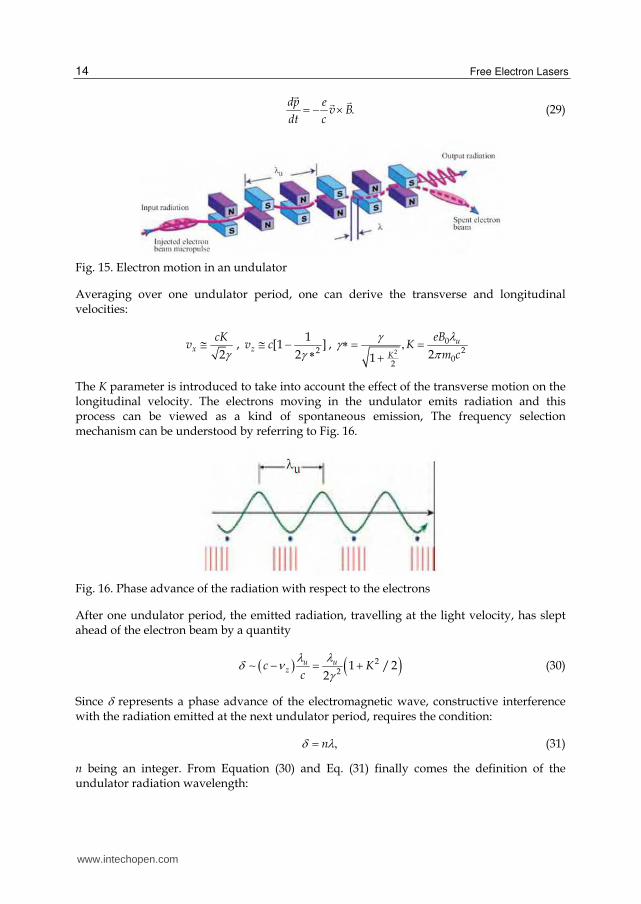
Fig. 15. Electron motion in an undulator

Averaging over one undulator period, one can derive the transverse and longitudinal velocities:

2x

cKv ,

2

1[1 ]

2zv c ,

2

02

02

21

u

K

eBK

m c

The K parameter is introduced to take into account the effect of the transverse motion on the longitudinal velocity. The electrons moving in the undulator emits radiation and this process can be viewed as a kind of spontaneous emission, The frequency selection mechanism can be understood by referring to Fig. 16.

Fig. 16. Phase advance of the radiation with respect to the electrons

After one undulator period, the emitted radiation, travelling at the light velocity, has slept ahead of the electron beam by a quantity

22

1 / 22

u uzc K

c

(30)

Since represents a phase advance of the electromagnetic wave, constructive interference with the radiation emitted at the next undulator period, requires the condition:

n (31)

n being an integer. From Equation (30) and Eq. (31) finally comes the definition of the undulator radiation wavelength:

www.intechopen.com


15

2

2(1 )

22u

n

K

n

(32)

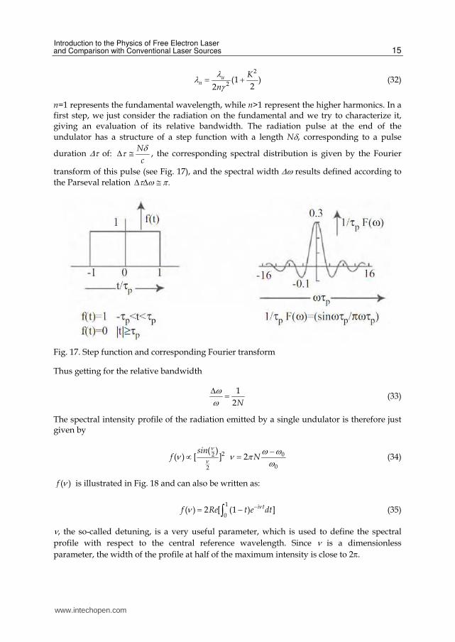
n=1 represents the fundamental wavelength, while n>1 represent the higher harmonics. In a first step, we just consider the radiation on the fundamental and we try to characterize it, giving an evaluation of its relative bandwidth. The radiation pulse at the end of the

undulator has a structure of a step function with a length N, corresponding to a pulse

duration of: N

c

, the corresponding spectral distribution is given by the Fourier

transform of this pulse (see Fig. 17), and the spectral width results defined according to

the Parseval relation

Fig. 17. Step function and corresponding Fourier transform

Thus getting for the relative bandwidth

1

2N

(33)

The spectral intensity profile of the radiation emitted by a single undulator is therefore just given by

22

2

( )( ) [ ]

sinf

0

0

2 N (34)

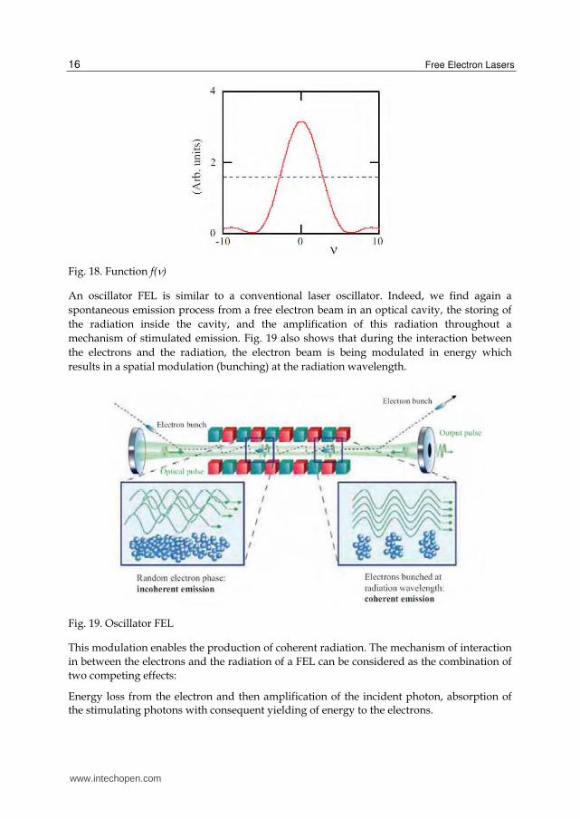
( )f is illustrated in Fig. 18 and can also be written as:

1

0( ) 2 [ (1 ) ]i tf Re t e dt (35)

, the so-called detuning, is a very useful parameter, which is used to define the spectral

profile with respect to the central reference wavelength. Since is a dimensionless

parameter, the width of the profile at half of the maximum intensity is close to 2.

www.intechopen.com


16

Fig. 18. Function f()

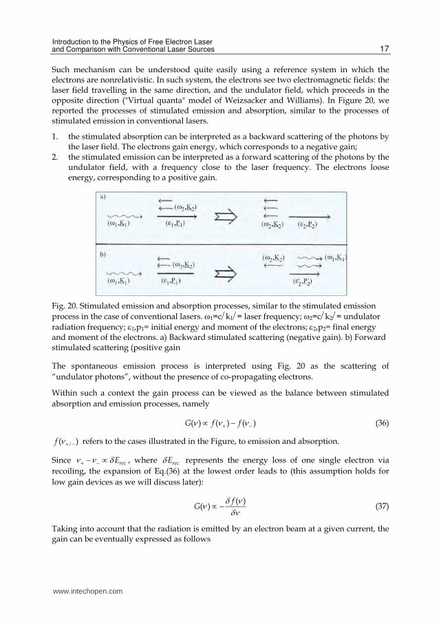
An oscillator FEL is similar to a conventional laser oscillator. Indeed, we find again a

spontaneous emission process from a free electron beam in an optical cavity, the storing of

the radiation inside the cavity, and the amplification of this radiation throughout a

mechanism of stimulated emission. Fig. 19 also shows that during the interaction between

the electrons and the radiation, the electron beam is being modulated in energy which

results in a spatial modulation (bunching) at the radiation wavelength.

Fig. 19. Oscillator FEL

This modulation enables the production of coherent radiation. The mechanism of interaction

in between the electrons and the radiation of a FEL can be considered as the combination of

two competing effects:

Energy loss from the electron and then amplification of the incident photon, absorption of the stimulating photons with consequent yielding of energy to the electrons.

www.intechopen.com


17

Such mechanism can be understood quite easily using a reference system in which the electrons are nonrelativistic. In such system, the electrons see two electromagnetic fields: the laser field travelling in the same direction, and the undulator field, which proceeds in the opposite direction ("Virtual quanta" model of Weizsacker and Williams). In Figure 20, we reported the processes of stimulated emission and absorption, similar to the processes of stimulated emission in conventional lasers.

1. the stimulated absorption can be interpreted as a backward scattering of the photons by the laser field. The electrons gain energy, which corresponds to a negative gain;

2. the stimulated emission can be interpreted as a forward scattering of the photons by the undulator field, with a frequency close to the laser frequency. The electrons loose energy, corresponding to a positive gain.

Fig. 20. Stimulated emission and absorption processes, similar to the stimulated emission

process in the case of conventional lasers. 1=ck1= laser frequency; 2=ck2= undulator

radiation frequency; 1,p1= initial energy and moment of the electrons; 2,p2= final energy and moment of the electrons. a) Backward stimulated scattering (negative gain). b) Forward stimulated scattering (positive gain

The spontaneous emission process is interpreted using Fig. 20 as the scattering of

“undulator photons”, without the presence of co-propagating electrons.

Within such a context the gain process can be viewed as the balance between stimulated

absorption and emission processes, namely

( ) ( ) ( )G f f (36)

( )f refers to the cases illustrated in the Figure, to emission and absorption.

Since recE , where recE represents the energy loss of one single electron via

recoiling, the expansion of Eq.(36) at the lowest order leads to (this assumption holds for

low gain devices as we will discuss later):

( )

( )f

G (37)

Taking into account that the radiation is emitted by an electron beam at a given current, the gain can be eventually expressed as follows

www.intechopen.com


18

1

0 0 0

( )( ) 2 (1 ) ( )

fG g g t t sin t dt

, 3 20

0

4 ( ) ( )u b

J Ng K f

I

3

40

0

41 7045 10em c

I AZ c e

,2 2

0 12 2( ) ( )2(1 ) 2(1 )

b

K Kf J J

K K

2

KK (38)

0g is the small signal gain coefficient, 0I the Alfven current. The gain curve is reported in

Fig. 21 (one can note that the maximum of the gain does not correspond to the maximum of

the spontaneous emission intensity, but located at 0 2.6). J is the current density of the

electron beam and bf the Bessel factor which takes into account the non-perfectly sinusoidal

trajectory of the electrons in the linear polarized undulator.

Fig. 21. FEL gain curve

It is worth mentioning that the gain curve is asymmetric. It consists of one part of positive

gain and one part of absorption where the electrons, instead of giving energy to the

radiation, absorb some energy from the radiation.

Now that the existence of a gain is clarified, we will determine the saturation intensity. The

FEL process consists in a power transfer from the electron beam to the laser. The gain curve

is asymmetric but the FEL process is maintained until the Kinematic conditions are such that

a positive gain is guaranteed and that a sort of saturation is reached. The energy loss can be

deduced from the width of the positive gain region, related to the detuning parameter (see

Fig. 33 and Eq. (36)) by:

4 2N

(39)

This equation yields the energy variation of the electron beam induced by the FEL interaction:

1

2N

(40)

www.intechopen.com


19

We finally get the expression of the power, transferred from the radiation to the electrons (see Eq. (27)):

2

EL

PP

N (41)

According to what we discussed for conventional lasers and assuming that a similar dynamics is valid in the case of FEL, the saturation intensity can be expressed as:

02E

S

II

Ng , E

J EI

e

or in more practical units:

2 4 22

1[ ] 6 9312 10 ( ) ( [ ] )

2S u b

MWI cm K f

Ncm

(42)

In conclusion, we demonstrated that an oscillator FEL behaves like a conventional oscillator laser and therefore that most of the relevant theoretical description can be applied to the FEL.

4. FEL Oscillator model

In the former paragraph, we have shown a full parallel (in terms of gain and saturation intensity) between FEL and conventional lasers. Pursuing the analogy we can write the saturation of the FEL gain as (we impose an upper limit on the small signal gain coefficient to fix the limit of validity of this treatment)

0 0

( ) ,( )

0.85 , for 0.3

M

s

M

G IG X X

F X I

G g g

(43)

MG represents the maximum gain calculated at 0 2.6 and:

2( ) 1 1 2( 2 1) 3 2 2F X X X (44)

One can notice that in the case of the FEL, the saturation results slightly different from the conventional laser (presence of a quadratic term), but this is just a technical detail which does not modify the physics of the process. The use of rate equations as defined in Eq .(9) enables to obtain the evolution of the laser power in the cavity as

1 [(1 ) ( ) ]r r r rI I G X I (45)

As already seen, the signal increases initially in the exponential mode, then the increase slows down and finally stops (or nearly) when the gain equals the losses. The equilibrium

power in the cavity is obtained from the condition 1r rI I , which implies:

( )1

eG X (46)

www.intechopen.com


20

Together with Eq. (43) and (44), this leads to the expression of the equilibrium intensity in the cavity:

1

( 2 1)( 1)e M SI G I

(47)

The solution of Eq. (45), (46) and (47) can be written as:

01 0

[(1 )( 1)]

1 [(1 )( 1)] 1e

rM

r I rMI

GI I

G

(48)

0I is the initial radiation intensity, due for instance to the spontaneous emission. An

example of evolution of the laser signal in the cavity is presented in Fig. 22.

Fig. 22. Example of FEL signal evolution in the cavity up to saturation. Comparison between simulation (continuous line) and analytic calculation (dotted line). The lower curve represents the gain reduction due to the increase of the intracavity intensity.

The evolution is typically sigmoidal, as in the case of the conventional lasers.

We discuss the mechanism of mode-locking in the case of oscillator FEL. From the gain curve, whose width is given by:

( )2

FEL

cf

N (49)

can be retrieved the number of coupled modes:

( )

( )FEL

me

f LN

f N (50)

www.intechopen.com


21

It is worth noticing that such value is inversely proportional to the slippage N. The physical meaning of this relation will be discussed later. In the absence of a specific mechanism of coupling of the longitudinal modes, the oscillator FEL modes also oscillate independently producing a fluctuating output radiation. But in the case of oscillator FEL, there is a natural coupling mechanism, resulting from the electron packets themselves, delivered by the accelerator with a pulse train structure of finite duration.

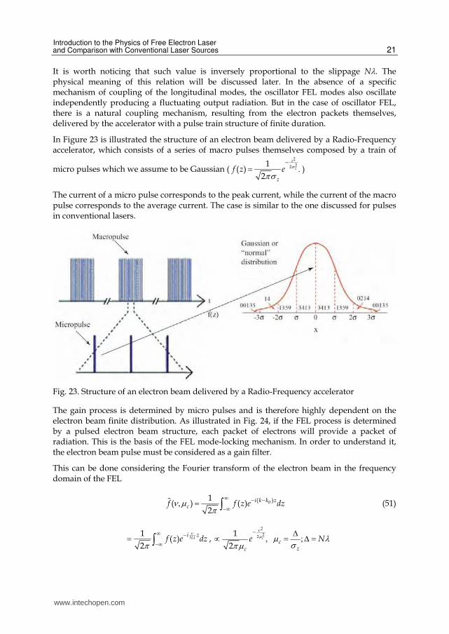
In Figure 23 is illustrated the structure of an electron beam delivered by a Radio-Frequency accelerator, which consists of a series of macro pulses themselves composed by a train of

micro pulses which we assume to be Gaussian (

2

221( )

2

z

z

z

f z e )

The current of a micro pulse corresponds to the peak current, while the current of the macro pulse corresponds to the average current. The case is similar to the one discussed for pulses in conventional lasers.

Fig. 23. Structure of an electron beam delivered by a Radio-Frequency accelerator

The gain process is determined by micro pulses and is therefore highly dependent on the electron beam finite distribution. As illustrated in Fig. 24, if the FEL process is determined by a pulsed electron beam structure, each packet of electrons will provide a packet of radiation. This is the basis of the FEL mode-locking mechanism. In order to understand it, the electron beam pulse must be considered as a gain filter.

This can be done considering the Fourier transform of the electron beam in the frequency domain of the FEL

0( )1( ) ( )

2

i k k zcf f z e dz

(51)

1( )

2N

i zf z e dz

,

2

221

2c

c

e

cz

N

www.intechopen.com


22

is referred as the slippage length. The Fourier transform of f(z) is Gaussian too and in the

following, we will use the normalized form:

2

221( )

2c

cc

f e

Fig. 24. Formation of a laser pulse from an electron beam pulse

The filter, representing the electron beam, is therefore regulated by the quantity c , referred

as longitudinal coupling coefficient. This quantity has an all-purpose physical meaning,

which will be discussed in detail later. Here, we just highlight that when c increases, the

number of coupled modes increases, and that for a continuous beam ( z ) the

operation becomes essentially single mode. The distribution derived from the former

equation becomes a Dirac peak. The gain "filtered" by the electron beam can be written in

terms of a convolution:

21 ( ) 2

0 0( ) ( ) ( ) 2 (1 ) ( ) ct

p c cG G y f y dy g t t sin t e dt (52)

It appears from this relation that for positive coupling coefficient values, the gain is

decreased, simply because there are more modes oscillating in phase, and according to Eq.

(52) that those coupled modes are within the rms band: c 5. FEL equations

The previous considerations are essentially qualitative, to make the forthcoming arguments quantitative we cast the FEL field evolution equation in the form

0 0( ) ida

i g a e dd

ni

n na a e , 2 28s

II

a (53)

www.intechopen.com


23

The previous equation can be exploited to specify the field growth before the saturation. It must be stressed that it contains something more, with respect to the considerations leading to the definition of the gain curve derived in the previous section, which were based on the assumption that the field remains constant during the interaction inside the undulator. Eq. (53) holds under more general assumptions, it includes the effects of high gain, i.e. the corrections associated to the fact that the field can vary significantly during the interaction.

The FEL gain is the relative variation of the input field in one interaction (

220

20

a aG

a

).

The FEL gain curve can be derived from Eq. (88), using the low gain approximation

satisfactory for small signal gain coefficient values lower than 30% . For higher values, the

gain curve is no more anti-symmetric. The maximum gain is no more simply proportional to

0g and further corrections should be included, namely

2 3 30 0 0 0 0( ) 0 85 0 192 4 23 10 g 10MG G g g g g (54)

Eq. (53) considers an ideal electron beam, i.e. one with all electrons at the same energy. In reality, the energy distribution of the electron beam can be assumed

Gaussian:2

221( )

2f e

, 0

0

, with being the electron beam relative energy

spread. The energy distribution induces an analogous distribution in the frequency domain of the FEL gain:

2

22( )1( )

2 ( )f e

, 4N (55)

Following the same procedure of convolution, as in the case of the longitudinal modes distribution, Eq. (53) is modified as following:

( ')'( ') 'ia

i g a e e d

になにどど (56)

The reduction of the gain due to the energy distribution is similar to the reduction of the

gain due to the inhomogeneous broadening in conventional lasers and the parameter is

one of the inhomogeneous broadening parameter of the FEL. The reduction of the gain due

to such effect can be quantified according to 2

11 1 7

MGG

. Further sources of

inhomogeneous broadening will not be considered here.

The inclusion of the electron packet shape and of the consequent optical pulse phenomenology can be done by taking into account the fact that the photon packet, having a higher velocity that the electrons, slips over the electron packet (see Fig. 38). Therefore, Equation (56) should be modified according to:

( ')

'( , )( ) ( ', ') 'ia z

i g z a z e e d

になにどど (57)

www.intechopen.com


24

0( )g z is the small signal gain coefficient which takes into account the electrons

distribution ( )f z ,

2

221( )

2

z

z

z

f z e and the slippage. The former equation is sufficiently

general to describe the dynamics of the pulse propagation with the effects of a high gain.

The coupling parameter c has an additional physical meaning which is worth mentioning:

it measures the overlapping of the electron beam with the photon beam. A very short electron beam remains superimposed to the photon beam for a very short time, which drives another reduction of the gain. The reduction of the gain due to the multi-mode

coupling and spatial overlap can be quantified as following4: 13

1M

c

GG .

An important aspect of the FEL dynamics is the non-linear harmonic generation, resulting from the bunching mechanism, which itself is a consequence of the energy modulation mechanism (see Fig. 25). When the electrons are micro-bunched at a wavelength which corresponds to a submultiple of the fundamental wavelength, coherent emission is produced at higher order harmonics, throughout the mechanism of nonlinear harmonic generation.

Fig. 25. Bunching mechanism induced by the FEL interaction. Bunching is performed at the resonant wavelength and on higher harmonics, allowing radiation production on the fundamental and higher harmonics

The intra cavity evolution of the fundamental and of the higher order harmonics is presented in Fig. 26.

4Both Eqs. (97) and (100) are valid in the case of small gain ( 0g 0.3). For more general hypothesis, the

expressions are slightly more complicated and will not be reported here for simplicity.

www.intechopen.com


25

Fig. 26. Example of intra cavity evolution of the fundamental and of the high order harmonics (third and fifth). The Figure also reports the energy spread increase. Continuous lines: numerical calculation. Dashed line: analytical approximation

The dynamics of the process is understood as follows: the fundamental increases, until it

reaches a sufficiently high power level to induce a bunching, that can lead to non-linear

harmonic generation. The saturation mechanism comes from the combined effects of the

energy loss and energy spread increase of the electron beam due to the same interaction.

The maximum harmonic power is related to the maximum of the fundamental power

according to5:

03

1 1

2 2 4E

n n

n n PP g

Nn

(58)

where 0 ng is the small signal gain coefficient of the harmonic n . Note that the coefficient

4EP

N is the maximum power LP achievable on the fundamental. The higher order harmonics,

opposite to the fundamental, are not stored in the cavity. Therefore the powers presented in

Fig. 26 are relative to the harmonic generation in one single round trip.

The non-linear harmonic generation mechanism is similar to the frequency-mixing mechanism in the case of non-linear optics. Eq. (58) can be understood as the non-linear response of the medium (the electron beam) to the laser electric field, so that it can then be written in terms of amplitude of the harmonics electric field:

5Note that in the linear polarized undulators, radiation is emitted on-axis only at odd order harmonics (3,5…)

www.intechopen.com


26

n n LE E (59)

0

3

1

2 2

nn

g n n

n

Before concluding this paragraph, we will describe the profile of the pulses in a FEL oscillator and the method which can be implemented to shape the pulses simply using the cavity parameters.

7. Self amplified spontaneous FEL

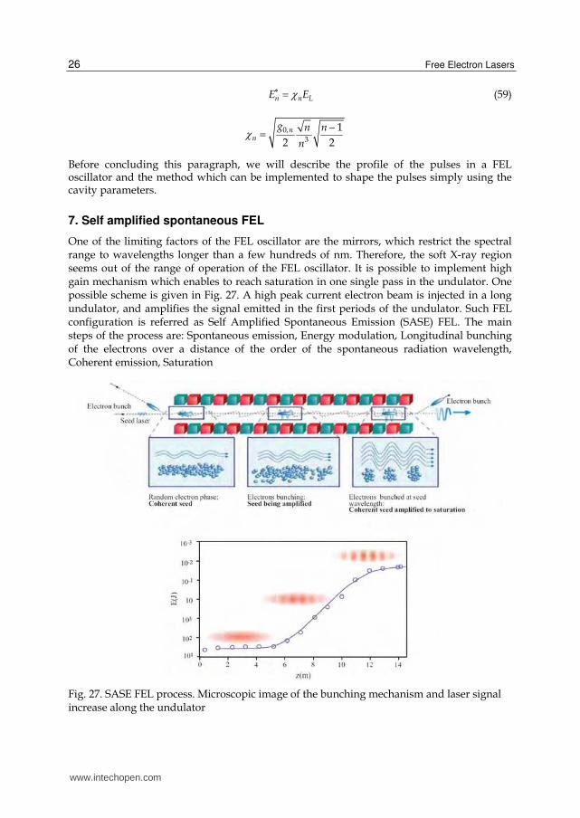
One of the limiting factors of the FEL oscillator are the mirrors, which restrict the spectral range to wavelengths longer than a few hundreds of nm. Therefore, the soft X-ray region seems out of the range of operation of the FEL oscillator. It is possible to implement high gain mechanism which enables to reach saturation in one single pass in the undulator. One possible scheme is given in Fig. 27. A high peak current electron beam is injected in a long undulator, and amplifies the signal emitted in the first periods of the undulator. Such FEL configuration is referred as Self Amplified Spontaneous Emission (SASE) FEL. The main steps of the process are: Spontaneous emission, Energy modulation, Longitudinal bunching of the electrons over a distance of the order of the spontaneous radiation wavelength, Coherent emission, Saturation

Fig. 27. SASE FEL process. Microscopic image of the bunching mechanism and laser signal increase along the undulator

www.intechopen.com


27

In order to understand these steps, we go back to the integral form of the FEL equations (see Eq. (53) ), which can be rewritten as follows:

'( ') 'i iae i g a e d

どど (60)

20 ˆ [ ( ) ]i ida

e i g a eDd

2D indicates an integration (or a negative derivative) repeated twice.

We also used the following Cauchy equality for the integrations

( 1

0

1ˆ ( ) ( ) ( )

( 1)

xn nx f x x f dD

n ,

1

10 0ˆ ( ) ( )

nx xnn nx f x dx dx f xD

).

Deriving both parts of Eq. (60) with respect to the temporal variables, the former integral equation can be transformed into an ordinary third order equation:

3 2 20ˆ ˆ ˆ( 2 ) ( ) ( )i a i g aD D D

ˆn

nn n

dD

d (61)

20 0 0 0ˆ ˆ0 0a a a aD D

The solution of this equation is obtained with a standard method and can be written as following:

23 3

( )0( ) (( )3( )

ii p qaa e p q e

p q

6( ) 3

2(2 ) ( ( ( ) )6

i p qp q e cosh p q

3 3

( ( ) )6

i sinh p qp q

(62)

1 13 31 1

( ) ( )2 2

p r d q r d

3 30 0 027 2 27 27 4r g d g g

It is not so easy to handle from the analytical point of view, nor easy to interpret from the

physical point of view. A more transparent form can be obtained with =0 in Eq. (61). This

is justified since we are considering solutions with a high gain, and that since in this case,

www.intechopen.com


28

maximum gain is reached for small values of the detuning parameter. In the =0 case, Eq.

(61) becomes much more simple:

30ˆ ( ) ( )a i g aD (63)

The general solution is a linear combination of the three roots which is given by:

2 2

0 0

( ) ( ) j

j j jj j

a a R a e

(64)

j are the three complex roots of 13

0( )g . The solution is then finally given by:

1

330 2

( )( )

ga e

(65)

In addition, using u

zN , the former relation becomes:

2( )zLGa z e

4 3u

GL 1

303

1( )

4

g

N

(66)

GL is referred as the gain length, while is referred as the Pierce parameter and constitutes

one of the fundamental parameters of the SASE FEL. Finally, including the three roots in the

expression, the evolution of the power in the small signal gain regime is given by:

20( ) ( )a A z a ,

1 1 1

1 3( ) (3 2 ( ) 4 ( ) ( ))

9 2 2g g g

z z zA z cosh cos cosh

L L L

This relation enables to describe the initial zone of non-exponential growth.

The former equation only describes the intensity increase of the laser, not its saturation. The physical mechanism which determines the saturation is not different from the one which has been previously discussed in the case of the oscillators. To simplify the treatment, we assume that the evolution is just the one relative to the exponential growth, so that we can write the differential equation relative to the growth process as following:

( ) ( )( ) (1 )

g F

d P z P zP z

dz L P , 0(0)P P

A quadratic non linearity has been added in order to take into account the effects of saturation. FP indicates the final power in the saturation regime, that we will specify later.

The solution of the former equation can be obtained easily, using the transformation:

1 1 1

1 1 1( ) ( ( ) ) ( )

( )g F

dT z T z T z

dz L P P z and can be written:

0

0( )9 1 ( 1)

g

g

F

z L

z LP

P

P eP z

e

(67)

www.intechopen.com


29

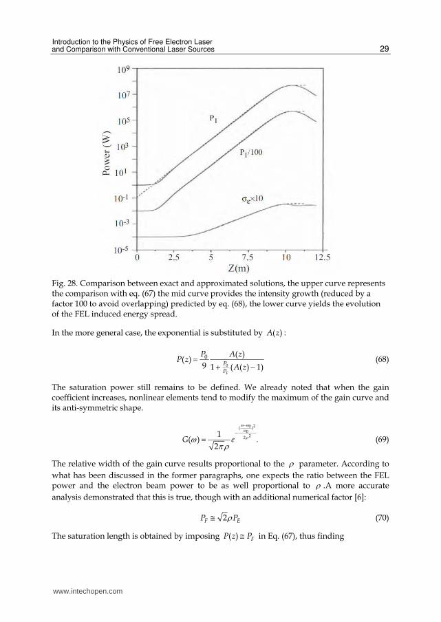
Fig. 28. Comparison between exact and approximated solutions, the upper curve represents the comparison with eq. (67) the mid curve provides the intensity growth (reduced by a factor 100 to avoid overlapping) predicted by eq. (68), the lower curve yields the evolution of the FEL induced energy spread.

In the more general case, the exponential is substituted by ( )A z :

0

0 ( )( )

9 1 ( ( ) 1)F

P

P

P A zP z

A z (68)

The saturation power still remains to be defined. We already noted that when the gain coefficient increases, nonlinear elements tend to modify the maximum of the gain curve and its anti-symmetric shape.

20( )0

221

( )2

G e

(69)

The relative width of the gain curve results proportional to the parameter. According to

what has been discussed in the former paragraphs, one expects the ratio between the FEL power and the electron beam power to be as well proportional to .A more accurate

analysis demonstrated that this is true, though with an additional numerical factor [6]:

2F EP P (70)

The saturation length is obtained by imposing ( ) FP z P in Eq. (67), thus finding

www.intechopen.com


30

0

9ln F

F g

PZ L

P

(71)

Corresponding to the number of periods 1FN

To get some numerical examples, we can note that if one limits the undulator length to a few tens of meters, given that the undulator period is of the order of a few centimetres and that

8010FP P , the value of the results around 310 . A comparison between “analytical” and

numerical predictions is given in Fig. 28.

8. SASE FEL and coherence

In the former paragraphs, we saw that the longitudinal coherence in FEL oscillators operated with short electron bunches, is guaranteed by the mode-locking mechanism. In the case of the FEL operated in the SASE regime, since there is no optical cavity, we can no longer talk about longitudinal modes, strictly speaking. Nevertheless, we can repeat the same argumentation on the filter properties of the electron beam to understand if something analogous to mode-locking can be defined for the cases of FEL operated in the SASE regime. As we already saw in the case of the oscillators, the effect of mode-locking is guaranteed in the interaction region where the electrons see a field with constant phase. This region is limited to one slippage length. We repeat the same procedure of Fourier transform which

enabled to obtain Eq. (52). Using for the frequency domain the variable 0

0

and

changing the variable for the space domain according to zc

, being the slippage length,

we obtain the integral:

1( ) ( )

2

if f e d (72)

from which:

2

221( )

2c

c

f e

c

z

We used the approximation 1 N

. The former relation ensures that a coherence length cl

exists and that it is around (a more correct definition will be given later). If the

electron beam length is about the coherence length, there would not be any problem of longitudinal coherence because all the modes inside the gain curve would be naturally

coupled. Since in practical cases z and since there is no clear definition of the

longitudinal modes, we should define "macro modes", i.e. a sort of extension of the longitudinal modes. The number of "macro modes" is given by:

zL

c

Ml

(73)

www.intechopen.com


31

Such macro modes introduced in the FEL Physics at the end of the 70’s by Dattoli and

Renieri are referred as supermodes (see [4] and references therein).

Each of these modes have a spatial distribution given by:

2

221( )

2

z

lc

c

m z el

4 3

cz

l

The relevant Fourier transform ( )m provide us with the frequency distribution. The total

spectrum is given by:

1

( ) ( )LM

nn

S m

(74)

The phase of each component is totally random. The spatial distribution of the optical pulse

is given by the Fourier transform of the spectrum and the results is shown in Fig. 29.

Fig. 29. Temporal and spectral distribution of the SASE FEL

Each randomly phased supermode makes one optical pulse which results in a series of

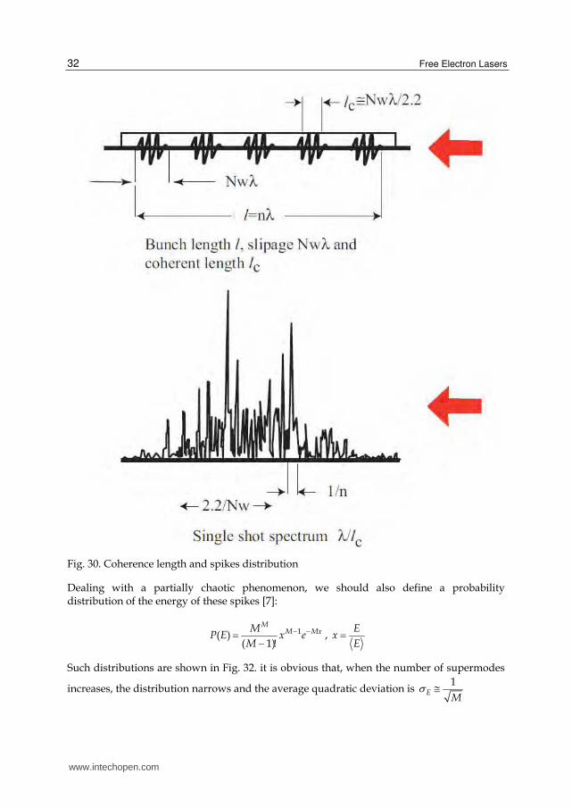
spikes separated by a fixed distance: the coherence length (see Fig. 30).

The evolution of each supermode is nearly independent from the others. There is only the

slippage which enables to create a coherence zone (of the same order of the coherence

length) and produces a sort of smoothing of the chaos, while the field increases along the

undulator (see Fig. 31).

www.intechopen.com


32

Fig. 30. Coherence length and spikes distribution

Dealing with a partially chaotic phenomenon, we should also define a probability distribution of the energy of these spikes [7]:

1( )( 1)

MM MxM

P E x eM

,E

xE

Such distributions are shown in Fig. 32. it is obvious that, when the number of supermodes

increases, the distribution narrows and the average quadratic deviation is 1

EM

www.intechopen.com


33

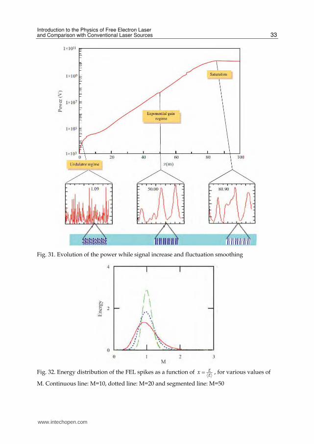
Fig. 31. Evolution of the power while signal increase and fluctuation smoothing

Fig. 32. Energy distribution of the FEL spikes as a function of EE

x , for various values of

M. Continuous line: M=10, dotted line: M=20 and segmented line: M=50

www.intechopen.com


34

Clarified the notion of longitudinal coherence, we move on to the definition of the transverse coherence. As previously, the problem of the definition of a transverse coherence results from the fact that there is no more optical cavity, which prevent us from defining strictly speaking transverse modes. We should note that in the high gain case, we will no longer be able to talk about free modes but guided modes, because of the strong distortion in the propagation caused by the interaction itself. An example of such behaviour is given in Fig. 33.

Fig. 33. a) Gaussian mode and b) guided mode

The Figure also illustrates the gain guiding mechanism, which becomes relevant as soon as the Rayleigh length becomes longer than the gain length. It is obvious that even in this case the parameter plays a fundamental role. Indeed, the condition for the guided modes can

be written as follows:

2 2

04 3u

w

(75)

Without optical cavity, the waist is essentially related to the transverse section of the electronic beam.

Before concluding this section, we note that the effects of inhomogeneous broadening and relative reduction of the gain in SASE can be treated using the same procedure given in the case of a FEL oscillator. In the case of energy spread, the parameter which quantifies the importance of the associated inhomogeneous broadening is

2 (76)

The macroscopic consequence is an increase of the saturation length given by:

gg LL 231 0 185

2 (77)

www.intechopen.com


35

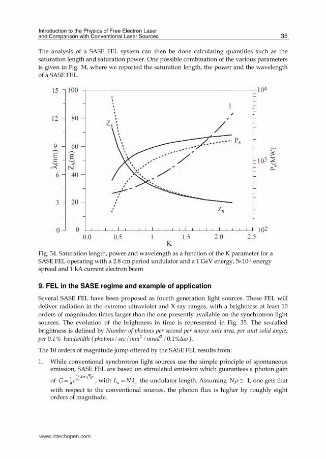
The analysis of a SASE FEL system can then be done calculating quantities such as the

saturation length and saturation power. One possible combination of the various parameters

is given in Fig. 34, where we reported the saturation length, the power and the wavelength

of a SASE FEL.

Fig. 34. Saturation length, power and wavelength as a function of the K parameter for a

SASE FEL operating with a 2.8 cm period undulator and a 1 GeV energy, 510-4 energy spread and 1 kA current electron beam

9. FEL in the SASE regime and example of application

Several SASE FEL have been proposed as fourth generation light sources. These FEL will

deliver radiation in the extreme ultraviolet and X-ray ranges, with a brightness at least 10

orders of magnitudes times larger than the one presently available on the synchrotron light

sources. The evolution of the brightness in time is represented in Fig. 35. The so-called

brightness is defined by Number of photons per second per source unit area, per unit solid angle,

per 0.1% bandwidth ( 2 2 0 1photons sec mm mrad % ).

The 10 orders of magnitude jump offered by the SASE FEL results from:

1. While conventional synchrotron light sources use the simple principle of spontaneous emission, SASE FEL are based on stimulated emission which guarantees a photon gain

of 4 31

9

Lu

uG e , with u uL N the undulator length. Assuming N 1, one gets that

with respect to the conventional sources, the photon flux is higher by roughly eight orders of magnitude.

www.intechopen.com


36

2. The conventional sources use electron beams accelerated in a storage ring, while SASE FEL use an electron beam accelerated in a LINAC (linear accelerator) of high energy. The transverse dimensions of the emitting source (the electron beam) is therefore 100 times smaller in the case of the SASE FEL that in the case of the synchrotron sources. According to what has been said in (1) and given that the brightness is inversely proportional to the transverse section of the beam, the magnification factor reaches ten orders of magnitude.

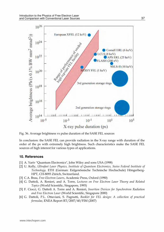
Another interesting aspect of the SASE FEL is the pulse duration of the radiation: as illustrated in Fig. 36, SASE FEL can produce ultra-short radiation pulses.

Fig. 35. Evolution of the brilliance of the X-ray conventional sources over the years and perspectives offered by FEL sources

The shortness of the X-ray pulse is related to the duration of the current pulse, which

generated it. The electron beam length can be understood as follows. Assuming a maximum

charge of 1 nC ( 910 C) and given that a SASE FEL needs currents of at least 1 kA to obtain a

reasonable saturation length, it turns obvious that the duration of the electron beam should

be smaller than a few ps.

www.intechopen.com


37

Fig. 36. Average brightness vs pulse duration of the SASE FEL sources

In conclusion: the SASE FEL can provide radiation in the X-ray range with duration of the order of the ps with extremely high brightness. Such characteristics make the SASE FEL sources of high interest for various types of applications.

10. References

[1] A. Yariv "Quantum Electronics", John Wiley and sons USA (1998) [2] U. Kelly, Ultrafast Laser Physics, Institute of Quantum Electronics, Swiss Federal Institute of

Technology. ETH (German: Eidgenössische Technische Hochschule) Höngerberg- HPT, CH-8093 Zürich, Switzerland.

[3] C.A. Brau, Free-Electron Lasers, Academic Press, Oxford (1990) [4] G. Dattoli, A. Renieri, and A. Torre, Lectures on Free Electron Laser Theory and Related

Topics (World Scientific, Singapore, 1993) [5] F. Ciocci, G. Dattoli A. Torre and A. Renieri, Insertion Devices for Synchrotron Radiation

and Free Electron Laser (World Scientific, Singapore 2000) [6] G. Dattoli, P.L. Ottaviani, S. Pagnutti, Booklet for FEL design: A collection of practical

formulae, ENEA Report RT/2007/40/FIM (2007)

www.intechopen.com


38

[7] E.L. Saldin, E.A. Schneidmiller, M.V. Yurkov, The Physics of Free Electron Lasers, (Springer-Verlag Berlin 1999)

www.intechopen.com

Free Electron LasersEdited by Dr. Sandor Varro

ISBN 978-953-51-0279-3Hard cover, 250 pagesPublisher InTechPublished online 14, March, 2012Published in print edition March, 2012

InTech EuropeUniversity Campus STeP Ri Slavka Krautzeka 83/A 51000 Rijeka, Croatia Phone: +385 (51) 770 447 Fax: +385 (51) 686 166www.intechopen.com

InTech ChinaUnit 405, Office Block, Hotel Equatorial Shanghai No.65, Yan An Road (West), Shanghai, 200040, China

Phone: +86-21-62489820 Fax: +86-21-62489821

Free Electron Lasers consists of 10 chapters, which refer to fundamentals and design of various free electronlaser systems, from the infrared to the xuv wavelength regimes. In addition to making a comparison withconventional lasers, a couple of special topics concerning near-field and cavity electrodynamics, compact andtable-top arrangements and strong radiation induced exotic states of matter are analyzed as well. The controland diagnostics of such devices and radiation safety issues are also discussed. Free Electron Lasers providesa selection of research results on these special sources of radiation, concerning basic principles, applicationsand some interesting new ideas of current interest.

How to referenceIn order to correctly reference this scholarly work, feel free to copy and paste the following:

G. Dattoli, M. Del Franco, M. Labat, P. L. Ottaviani and S. Pagnutti (2012). Introduction to the Physics of FreeElectron Laser and Comparison with Conventional Laser Sources, Free Electron Lasers, Dr. Sandor Varro(Ed.), ISBN: 978-953-51-0279-3, InTech, Available from: http://www.intechopen.com/books/free-electron-lasers/free-electron-laser-devices-a-comparison-with-ordinary-laser-sources

© 2012 The Author(s). Licensee IntechOpen. This is an open access articledistributed under the terms of the Creative Commons Attribution 3.0License, which permits unrestricted use, distribution, and reproduction inany medium, provided the original work is properly cited.

http://creativecommons.org/licenses/by/3.0

introduction to the physics of free electron laser and...

Documents