introductions to erf z ª t â - wolfram research

Introductions to ErfIntroduction to the probability integrals and inverses

General

The probability integral (error function) erfHzL has a long history beginning with the articles of A. de Moivre

(1718–1733) and P.-S. Laplace (1774) where it was expressed through the following integral:

à ã-t2 â t.

Later C. Kramp (1799) used this integral for the definition of the complementary error function erfcHzL. P.-S.

Laplace (1812) derived an asymptotic expansion of the error function.

The probability integrals were so named because they are widely applied in the theory of probability, in both

normal and limit distributions.

To obtain, say, a normal distributed random variable from a uniformly distributed random variable, the inverse of

the error function, namely erf-1HzL is needed. The inverse was systematically investigated in the second half of the

twentieth century, especially by J. R. Philip (1960) and A. J. Strecok (1968).

Definitions of probability integrals and inverses

The probability integral (error function) erfHzL, the generalized error function erfHz1, z2L, the complementary error

function erfcHzL, the imaginary error function erfiHzL, the inverse error function erf-1HzL, the inverse of the general-

ized error function erf-1Hz1, z2L, and the inverse complementary error function erfc-1HzL are defined through the

following formulas:

erfHzL �2

Π à

0

z

ã-t2 â t

erfHz1, z2L � erfHz2L - erfHz1LerfcHzL �

2

Π à

z

¥

ã-t2 â t

erfiHzL �2

Π à

0

z

ãt2 â t

z � erfHwL �; w � erf-1HzLz2 � erfHz1, wL �; w � erf-1Hz1, z2Lz � erfcHwL �; w � erfc-1HzL.These seven functions are typically called probability integrals and their inverses.

Instead of using definite integrals, the three univariate error functions can be defined through the following infinite

series.

erfHzL �2

Π âk=0

¥ H-1Lk z2 k+1

k ! H2 k + 1LerfcHzL � 1 -

2

Π âk=0

¥ H-1Lk z2 k+1

k ! H2 k + 1LerfiHzL �

2

Π âk=0

¥ z2 k+1

k ! H2 k + 1L .

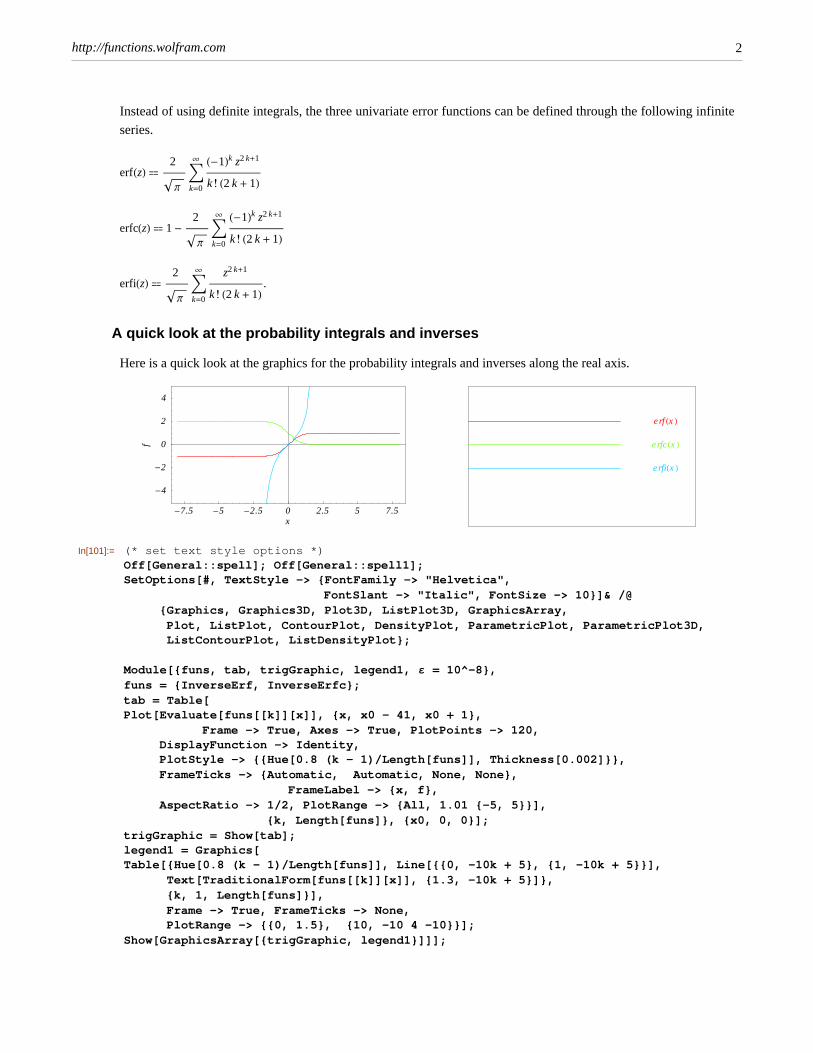
A quick look at the probability integrals and inverses

Here is a quick look at the graphics for the probability integrals and inverses along the real axis.

-7.5 -5 -2.5 0 2.5 5 7.5x

-4

-2

0

2

4

f

erf Hx LerfcHx LerfiHx L

In[101]:= (* set text style options *)Off[General::spell]; Off[General::spell1];SetOptions[#, TextStyle -> {FontFamily -> "Helvetica", FontSlant -> "Italic", FontSize -> 10}]& /@ {Graphics, Graphics3D, Plot3D, ListPlot3D, GraphicsArray, Plot, ListPlot, ContourPlot, DensityPlot, ParametricPlot, ParametricPlot3D, ListContourPlot, ListDensityPlot}; Module[{funs, tab, trigGraphic, legend1, ¶ = 10^-8},funs = {InverseErf, InverseErfc};tab = Table[Plot[Evaluate[funs[[k]][x]], {x, x0 - 41, x0 + 1}, Frame -> True, Axes -> True, PlotPoints -> 120, DisplayFunction -> Identity, PlotStyle -> {{Hue[0.8 (k - 1)/Length[funs]], Thickness[0.002]}}, FrameTicks -> {Automatic, Automatic, None, None}, FrameLabel -> {x, f}, AspectRatio -> 1/2, PlotRange -> {All, 1.01 {-5, 5}}], {k, Length[funs]}, {x0, 0, 0}];trigGraphic = Show[tab];legend1 = Graphics[Table[{Hue[0.8 (k - 1)/Length[funs]], Line[{{0, -10k + 5}, {1, -10k + 5}}], Text[TraditionalForm[funs[[k]][x]], {1.3, -10k + 5}]}, {k, 1, Length[funs]}], Frame -> True, FrameTicks -> None, PlotRange -> {{0, 1.5}, {10, -10 4 -10}}];Show[GraphicsArray[{trigGraphic, legend1}]]];

http://functions.wolfram.com 2

-1 -0.5 0 0.5 1x

-4

-2

0

2

4

ferf

-1 H0, xLerf

-1 H¥, -x L

Connections within the group of probability integrals and inverses and with other function groups

Representations through more general functions

The probability integrals erfHzL, erfHz1, z2L, erfcHzL, and erfiHzL are the particular cases of two more general func-

tions: hypergeometric and Meijer G functions.

For example, they can be represented through the confluent hypergeometric functions 1F1 and U:

erfHzL �2 z

Π 1F1

1

2;

3

2; -z2

erfHzL �z

z2

1 -1

Π ã-z2

U1

2,

1

2, z2

erfHz1, z2L �2 z2

Π1F1

1

2;

3

2; -z2

2 -2 z1

Π1F1

1

2;

3

2; -z1

2

erfHz1, z2L �z2

z22

1 -1

Π ã-z2

2U

1

2,

1

2, z2

2 -z1

z12

1 -1

Π ã-z1

2U

1

2,

1

2, z1

2

erfcHzL � 1 -2 z

Π 1F1

1

2;

3

2; -z2

erfcHzL �z

z2

1

Π ã-z2

U1

2,

1

2, z2 - 1 + 1

erfiHzL �2 z

Π 1F1

1

2;

3

2; z2

erfiHzL �z

-z2

1 -1

Π ãz2

U1

2,

1

2, -z2 .

Representations of the probability integrals erfHzL, erfHz1, z2L, erfcHzL, and erfiHzL through classical Meijer G func-

tions are rather simple:


erfHzL �z

ΠG1,2

1,1 z2

1

2

0, - 1

2

erf Hz1, z2L �1

Π z2 G1,2

1,1 z22

1

2

0, - 1

2

- z1 G1,21,1 z1

2

1

2

0, - 1

2

erfc HzL � 1 -z

ΠG1,2

1,1 z2

1

2

0, - 1

2

erfi HzL �z

ΠG1,2

1,1 -z2

1

2

0, - 1

2

.

The factor z in the last four formulas can be removed by changing the classical Meijer G functions to the general-

ized one:

erfHzL �1

Π G1,2

1,1 z,1

2

11

2, 0

erf Hz1, z2L �1

Π G1,2

1,1 z2,1

2

11

2, 0

- G1,21,1 z1,

1

2

11

2, 0

erfc HzL �1

Π G1,2

2,0 z,1

2

1

0, 1

2

erfi HzL � -ä

Π G1,2

1,1 ä z,1

2

11

2, 0

.

The probability integrals erfHzL, erfHz1, z2L, erfcHzL, and erfiHzL are the particular cases of the incomplete gamma

function, regularized incomplete gamma function, and exponential integral E:

erfHzL �z2

z 1 -

1

Π G

1

2, z2

erfHzL �z2

z 1 - Q

1

2, z2

erfHzL �z2

z-

z

Π E 1

2

Iz2M

erfHz1, z2L �z2

2

z2

1 -1

Π G

1

2, z2

2 -z1

2

z1

1 -1

Π G

1

2, z1

2

erfHz1, z2L �z2

2

z2

1 - Q1

2, z2

2 -z1

2

z1

1 - Q1

2, z1

2


erfHz1, z2L �z1

ΠE 1

2

Iz12M -

z2

Π E 1

2

Iz22M +

z22

z2

-z1

2

z1

erfcHzL � 1 -z2

z 1 -

1

Π G

1

2, z2

erfcHzL � 1 -z2

z 1 - Q

1

2, z2

erfcHzL � 1 -z2

z+

z

Π E 1

2

Iz2M

erfiHzL �-z2

z

1

Π G

1

2, -z2 - 1

erfiHzL �-z2

z Q

1

2, -z2 - 1

erfiHzL � --z2

z-

z

Π E 1

2

I-z2M.Representations through related equivalent functions

The probability integrals erfHzL, erfcHzL, and erfiHzL can be represented through Fresnel integrals by the following

formulas:

erfHzL � H1 + äL CH1 - äL z

Π- ä S

H1 - äL z

Π

erfcHzL � 1 - H1 + äL CH1 - äL z

Π- ä S

H1 - äL z

Π

erfiHzL � H1 - äL CH1 + äL z

Π- ä S

H1 + äL z

Π.

Representations through other probability integrals and inverses

The probability integrals and their inverses erfHzL, erfHz1, z2L, erfcHzL, erfiHzL, erf-1HzL, erf-1Hz1, z2L, and erfc-1HzL are

interconnected by the following formulas:

erfHzL � erfH0, zLerfHzL � 1 - erfcHzLerfHzL � -ä erfiHä zLerfIerf-1HzLM � z


erfIerf-1H0, zLM � z

erfIz1, erf-1Hz1, z2LM � z2

erfIerfc-1H1 - zLM � z

erfcHzL � erfHz, ¥LerfcHzL � 1 - erfHzLerfcHzL � 1 + ä erfiHä zLerfcIerf-1H1 - zLM � z

erfcIerf-1H¥, -zLM � z

erfcIerfc-1HzLM � z

erfiHzL � ä erfHä z, 0LerfiHzL � ä erfcHä zL - ä

erfiHzL � -ä erfHä zLerfiIä erf-1HzLM � ä z

erfiIä erf-1H0, zLM � ä z

erfiIä erfc-1H1 - zLM � ä z

erf-1HzL � erf-1H0, zLerf-1HzL � erfc-1H1 - zLerfc-1HzL � erf-1H¥, -zLerfc-1HzL � erf-1H1 - zL.

The best-known properties and formulas for probability integrals and inverses

Real values for real arguments

For real values of argument z, the values of the probability integrals erfHzL, erfHz1, z2L, erfc HzL, and erfi HzL are real.

For real arguments -1 < z < 1, the values of the inverse error function erf-1HzL are real; for real arguments

-1 < z1 < 1, -1 < z2 < 1, the values of the inverse of the generalized error function erf-1Hz1, z2L are real; and for

real arguments 0 < z < 2, the values of the inverse complementary error function erfc-1HzL are real.

Simple values at zero and one

The probability integrals erfHzL, erfHz1, z2L, erfcHzL, and erfiHzL, and their inverses erf-1HzL, erf-1Hz1, z2L, and erfc-1HzLhave simple values for zero or unit arguments:


erfH0L � 0

erfH0, 0L � 0

erfcH0L � 1

erfiH0L � 0

erf-1H0L � 0

erf-1H1L � ¥

erf-1H0, 0L � 0

erf-1H0, 1L � ¥

erf-1H1, 0L � 1

erfc-1H0L � ¥

erfc-1H1L � 0.

Simple values at infinity

The probability integrals erfHzL, erfcHzL, and erfiHzL have simple values at infinity:

erfH¥L � 1

erfcH¥L � 0

erfiH¥L � ¥.

Specific values for specialized arguments

In cases when z1 or z2 is equal to 0 or ¥, the generalized error function erfHz1, z2L and its inverse erf-1Hz1, z2L can

be expressed through the probability integrals erf HzL, erfc HzL, or their inverses by the following formulas:

erfHz, 0L � -erfHzLerfH0, zL � erfHzLerfHz, ¥L � erfcHzLerfH¥, zL � erfHzL - 1

erf-1H0, zL � erf-1HzLerf-1H¥, zL � erfc-1H-zL.Analyticity

The probability integrals erfHzL, erfcHzL, and erfiHzL, and their inverses erf-1HzL, and erfc-1HzL are defined for all

complex values of z, and they are analytical functions of z over the whole complex z-plane. The probability inte-

grals erfHzL, erfcHzL, and erfiHzL are entire functions with an essential singular point at z = ¥� , and they do not have

branch cuts or branch points.


The generalized error function erfHz1, z2L is an analytical function of z1 and z2, which is defined in C2. For fixed z1,

it is an entire function of z2. For fixed z2, it is an entire function of z1. It does not have branch cuts or branch points.

The inverse of the generalized error function erf-1Hz1, z2L is an analytical function of z1 and z2, which is defined in

C2.

Poles and essential singularities

The probability integrals erfHzL, erfcHzL, and erfiHzL have only one singular point at z = ¥� . It is an essential singular

point.

The generalized error function erfHz1, z2L has singular points at z1 = ¥� and z2 � ¥� . They are essential singular

points.

Periodicity

The probability integrals erfHzL, erfHz1, z2L, erfcHzL, and erfiHzL, and their inverses erf-1HzL, erf-1Hz1, z2L, and erfc-1HzLdo not have periodicity.

Parity and symmetry

The probability integrals erfHzL, erfHz1, z2L, and erfiHzL are odd functions and have mirror symmetry:

erf H-zL � -erf HzL erf Hz�L � erfHzLerf H-z1, -z2L � -erf Hz1, z2L erf Hz1, z2L � erfHz1, z2Lerfi H-zL � -erfi HzL erfi Hz�L � erfiHzL .

The generalized error function erfHz1, z2L has permutation symmetry:

erfHz1, z2L � -erfHz2, z1L.The complementary error function erfcHzL has mirror symmetry:

erfcHz�L � erfcHzL.Series representations

The probability integrals erfHzL, erfHz1, z2L, erfcHzL, and erfiHzL, and their inverses erf-1HzL and erfc-1HzL have the

following series expansions:

erfHzL µ2

Π z -

z3

3+

z5

10- ¼ �; Hz ® 0L

erfHzL �2

Π âk=0

¥ H-1Lk z2 k+1

k ! H2 k + 1LerfHz1, z2L µ

2

Π z2 -

z23

3+

z25

10- ¼ -

2

Π z1 -

z13

3+

z15

10- ¼ �; Hz1 ® 0L ì Hz2 ® 0L


erfHz1, z2L �2

Π âk=0

¥ H-1Lk Iz22 k+1 - z1

2 k+1Mk ! H2 k + 1L

erfcHzL µ 1 -2

Π z -

z3

3+

z5

10- ¼ �; Hz ® 0L

erfcHzL � 1 -2

Π âk=0

¥ H-1Lk z2 k+1

k ! H2 k + 1LerfiHzL µ

2

Π z +

z3

3+

z5

10+ ¼ �; Hz ® 0L

erfiHzL �2

Π âk=0

¥ z2 k+1

k ! H2 k + 1Lerf-1HzL �

1

2Π z +

Π z3

12+ OIz5M

erf-1HzL � âk=0

¥ ck

2 k + 1

Π

2 z

2 k+1

�; c0 � 1 í ck � âm=0

k-1 cm ck-1-mHm + 1L H2 m + 1Lerf-1Hz1, z2L µ erf-1Hz2L + ãerf-1Hz2L2

z1 + ã2 erf-1Hz2L2

erf-1Hz2L z12 + OIz1

3Merf-1Hz1, z2L µ z1 +

1

2 ãz1

2Π z2 +

Π z1

4ã2 z1

2z2

2 + OIz23M

erfc-1HzL �Π

2-Hz - 1L -

1

12Π Hz - 1L3 + OIHz - 1L5M

erfc-1HzL � -âk=0

¥ ck

2 k + 1

Π

2 Hz - 1L

2 k+1

�; c0 � 1 í ck � âm=0

k-1 cm ck-1-mHm + 1L H2 m + 1L .

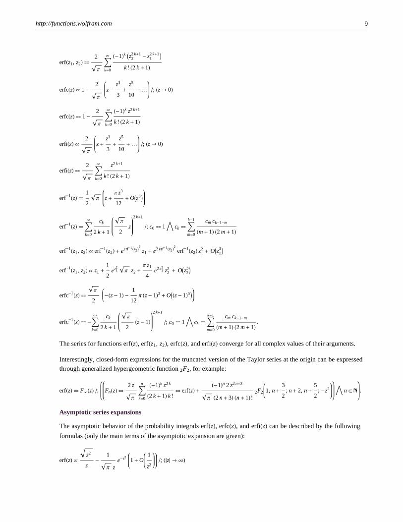
The series for functions erfHzL, erfHz1, z2L, erfcHzL, and erfiHzL converge for all complex values of their arguments.

Interestingly, closed-form expressions for the truncated version of the Taylor series at the origin can be expressed

through generalized hypergeometric function 2F2, for example:

erfHzL � F¥HzL �; FnHzL �2 z

Πâk=0

n H-1Lk z2 k

H2 k + 1L k !� erfHzL +

H-1Ln 2 z2 n+3

Π H2 n + 3L Hn + 1L !2F2 1, n +

3

2; n + 2, n +

5

2; -z2 í n Î N .

Asymptotic series expansions

The asymptotic behavior of the probability integrals erfHzL, erfcHzL, and erfiHzL can be described by the following

formulas (only the main terms of the asymptotic expansion are given):

erfHzL µz2

z-

1

Π z ã-z2

1 + O1

z2�; H z¤ ® ¥L


erfcHzL µ 1 -z2

z+

1

Π z ã-z2

1 + O1

z2�; H z¤ ® ¥L

erfiHzL µz

-z2

+1

Π z ãz2

1 + O1

z2�; H z¤ ® ¥L.

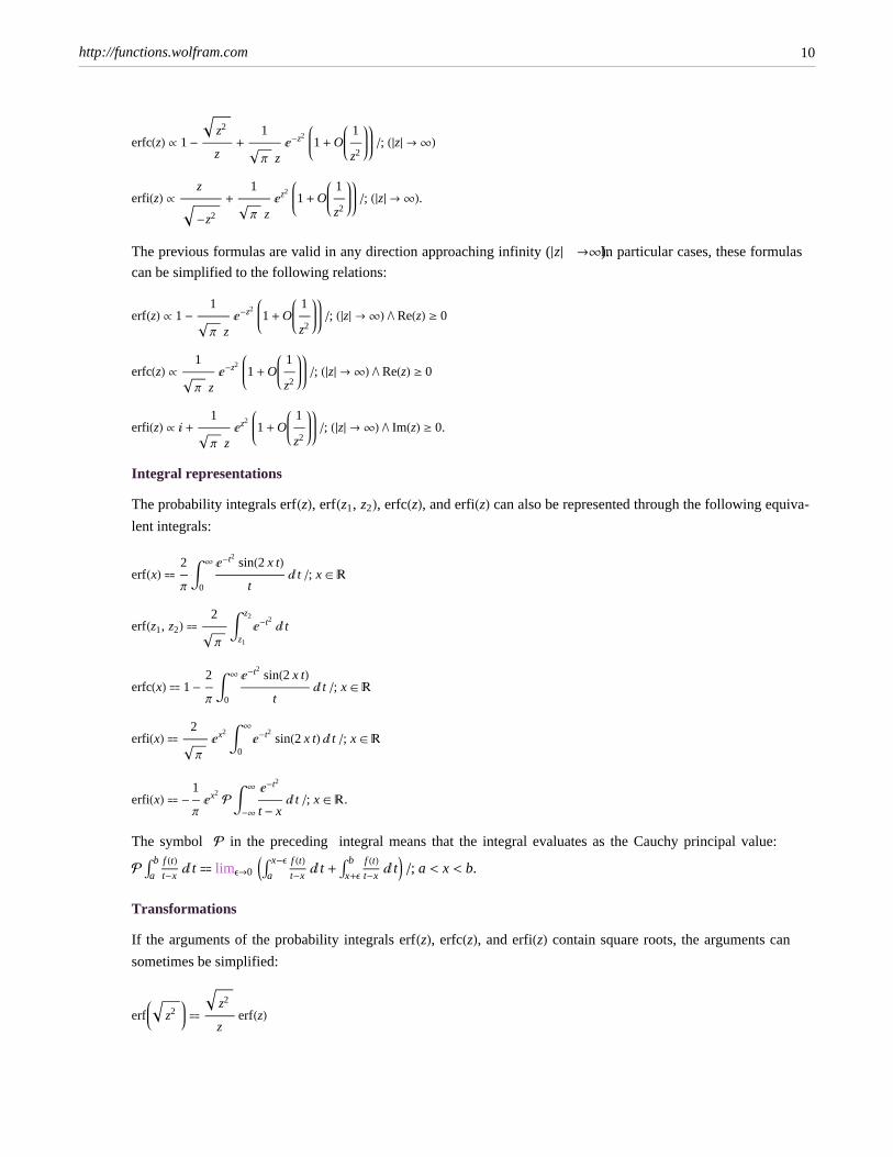
The previous formulas are valid in any direction approaching infinity ( z¤ ®¥). In particular cases, these formulas

can be simplified to the following relations:

erfHzL µ 1 -1

Π z ã-z2

1 + O1

z2�; H z¤ ® ¥L ß ReHzL ³ 0

erfcHzL µ1

Π z ã-z2

1 + O1

z2�; H z¤ ® ¥L ß ReHzL ³ 0

erfiHzL µ ä +1

Π z ãz2

1 + O1

z2�; H z¤ ® ¥L ß ImHzL ³ 0.

Integral representations

The probability integrals erfHzL, erfHz1, z2L, erfcHzL, and erfiHzL can also be represented through the following equiva-

lent integrals:

erfHxL �2

Π à

0

¥ ã-t2 sinH2 x tLt

â t �; x Î R

erfHz1, z2L �2

Π à

z1

z2

ã-t2 â t

erfcHxL � 1 -2

Π à

0

¥ ã-t2 sinH2 x tLt

â t �; x Î R

erfiHxL �2

Π ãx2 à

0

¥

ã-t2 sinH2 x tL â t �; x Î R

erfiHxL � -1

Π ãx2

P à-¥

¥ ã-t2

t - x â t �; x Î R.

The symbol P in the preceding integral means that the integral evaluates as the Cauchy principal value:

P Ùa

b f HtLt-x

â t � limΕ®0 JÙa

x-Ε f HtLt-x

â t + Ùx+Ε

b f HtLt-x

â tN �; a < x < b.

Transformations

If the arguments of the probability integrals erfHzL, erfcHzL, and erfiHzL contain square roots, the arguments can

sometimes be simplified:

erf z2 �z2

z erfHzL


erfc z2 � 1 -z2

z erfHzL

erfi z2 �z2

z erfiHzL.

Representations of derivatives

The derivative of the probability integrals erfHzL, erfHz1, z2L, erfcHzL, and erfiHzL, and their inverses erf-1HzL,erf-1Hz1, z2L, and erfc-1HzL have simple representations through elementary functions:

¶erf HzL¶z

�2 ã-z2

Π

¶erfHz1, z2L¶z1

� -2 ã-z1

2

Π

¶erfHz1, z2L¶z2

�2 ã-z2

2

Π

¶erfcHzL¶z

� -2 ã-z2

Π

¶erfiHzL¶z

�2 ãz2

Π

¶erf-1HzL¶z

�Π

2 ãerf-1HzL2

¶erf-1Hz1, z2L¶z1

� ãerf-1Hz1 ,z2L2-z1

2

¶erf-1Hz1, z2L¶z2

�Π

2 ãerf-1Hz1 ,z2L2

¶erfc-1HzL¶z

� -Π

2ãerfc-1HzL2

.

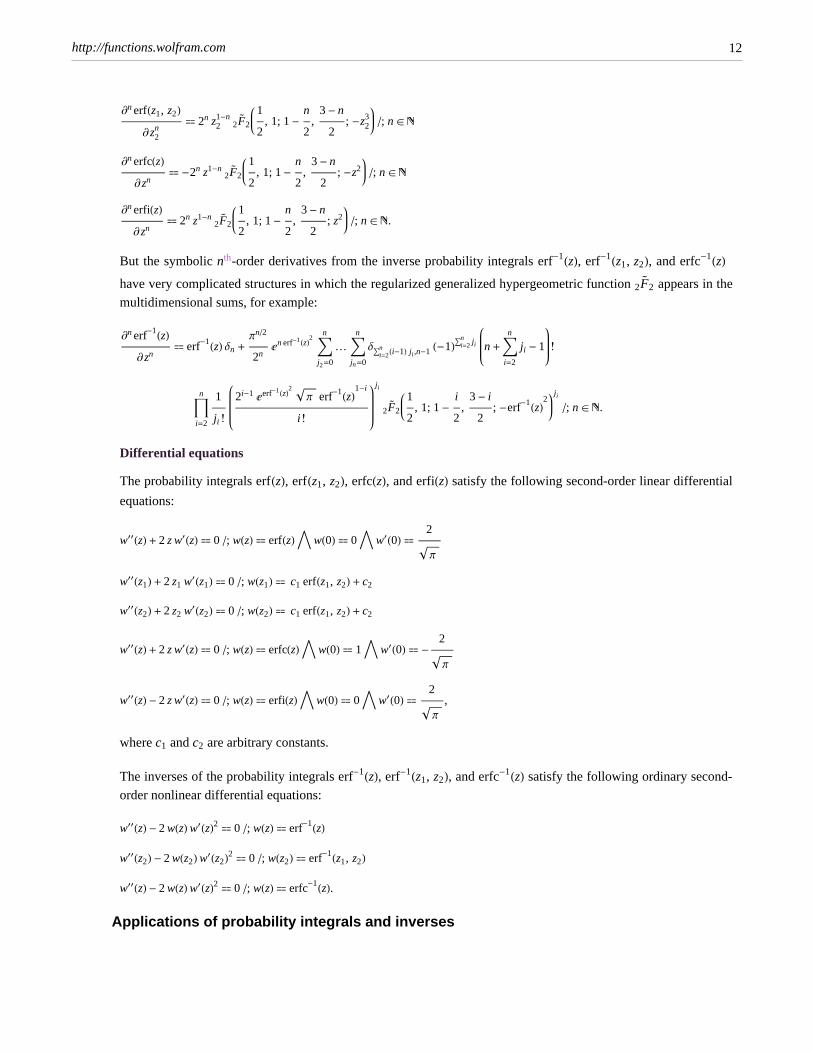
The symbolic nth-order derivatives from the probability integrals erfHzL, erfHz1, z2L, erfcHzL, and erfiHzL have the

following simple representations through the regularized generalized hypergeometric function 2F�

2:

¶n erf HzL¶zn

� 2n z1-n2F

�2

1

2, 1; 1 -

n

2,

3 - n

2; -z2 �; n Î N

¶n erfHz1, z2L¶z1

n� -2n z1

1-n2F

�2

1

2, 1; 1 -

n

2,

3 - n

2; -z1

3 �; n Î N


¶n erfHz1, z2L¶z2

n� 2n z2

1-n2F

�2

1

2, 1; 1 -

n

2,

3 - n

2; -z2

3 �; n Î N

¶n erfcHzL¶zn

� -2n z1-n2F

�2

1

2, 1; 1 -

n

2,

3 - n

2; -z2 �; n Î N

¶n erfiHzL¶zn

� 2n z1-n2F

�2

1

2, 1; 1 -

n

2,

3 - n

2; z2 �; n Î N.

But the symbolic nth-order derivatives from the inverse probability integrals erf-1HzL, erf-1Hz1, z2L, and erfc-1HzLhave very complicated structures in which the regularized generalized hypergeometric function 2F

�2 appears in the

multidimensional sums, for example:

¶n erf-1HzL¶zn

� erf-1HzL ∆n +Πn�22n

ãn erf-1HzL2 âj2=0

n

¼ âjn=0

n

∆Úi=2n Hi-1L ji ,n-1 H-1LÚi=2

n ji n + âi=2

n

ji - 1 !

äi=2

n 1

ji !

2i-1 ãerf-1HzL2

Π erf-1HzL1-i

i!

ji

2F�

2

1

2, 1; 1 -

i

2,

3 - i

2; -erf-1HzL2

ji �; n Î N.

Differential equations

The probability integrals erfHzL, erfHz1, z2L, erfcHzL, and erfiHzL satisfy the following second-order linear differential

equations:

w¢¢HzL + 2 z w¢HzL � 0 �; wHzL � erfHzL í wH0L � 0 í w¢H0L �2

Π

w¢¢Hz1L + 2 z1 w¢Hz1L � 0 �; wHz1L � c1 erfHz1, z2L + c2

w¢¢Hz2L + 2 z2 w¢Hz2L � 0 �; wHz2L � c1 erfHz1, z2L + c2

w¢¢HzL + 2 z w¢HzL � 0 �; wHzL � erfcHzL í wH0L � 1 í w¢H0L � -2

Π

w¢¢HzL - 2 z w¢HzL � 0 �; wHzL � erfiHzL í wH0L � 0 í w¢H0L �2

Π,

where c1 and c2 are arbitrary constants.

The inverses of the probability integrals erf-1HzL, erf-1Hz1, z2L, and erfc-1HzL satisfy the following ordinary second-

order nonlinear differential equations:

w¢¢HzL - 2 wHzL w¢HzL2 � 0 �; wHzL � erf-1HzLw¢¢Hz2L - 2 wHz2L w¢Hz2L2 � 0 �; wHz2L � erf-1Hz1, z2Lw¢¢HzL - 2 wHzL w¢HzL2 � 0 �; wHzL � erfc-1HzL.

Applications of probability integrals and inverses


Applications of probability integrals include solutions of linear partial differential equations, probability theory,

Monte Carlo simulations, and the Ewald method for calculating electrostatic lattice constants.


Copyright

This document was downloaded from functions.wolfram.com, a comprehensive online compendium of formulas

involving the special functions of mathematics. For a key to the notations used here, see

http://functions.wolfram.com/Notations/.

Please cite this document by referring to the functions.wolfram.com page from which it was downloaded, for

example:

http://functions.wolfram.com/Constants/E/

To refer to a particular formula, cite functions.wolfram.com followed by the citation number.

e.g.: http://functions.wolfram.com/01.03.03.0001.01

This document is currently in a preliminary form. If you have comments or suggestions, please email

[email protected].

© 2001-2008, Wolfram Research, Inc.


introductions to erf z ª t â - wolfram research

Documents