Chapter 3

Introduction to Sobolev

Spaces

Remark 3.1 Contents. Sobolev spaces are the basis of the theory of weak orvariational forms of partial differential equations. A very popular approach fordiscretizing partial differential equations, the finite element method, is based onvariational forms. In this chapter, a short introduction into Sobolev spaces will begiven. Recommended literature are the books Adams (1975); Adams and Fournier(2003) and Evans (2010).

3.1 Elementary Inequalities

Lemma 3.2 Inequality for strictly monotonically increasing function. Letf : R+ ∪ 0 → R be a continuous and strictly monotonically increasing functionwith f(0) = 0 and f(x) → ∞ for x→ ∞. Then, for all a, b ∈ R+ ∪ 0 it is

ab ≤

∫ a

0

f(x) dx+

∫ b

0

f−1(y) dy,

where f−1(y) is the inverse of f(x).

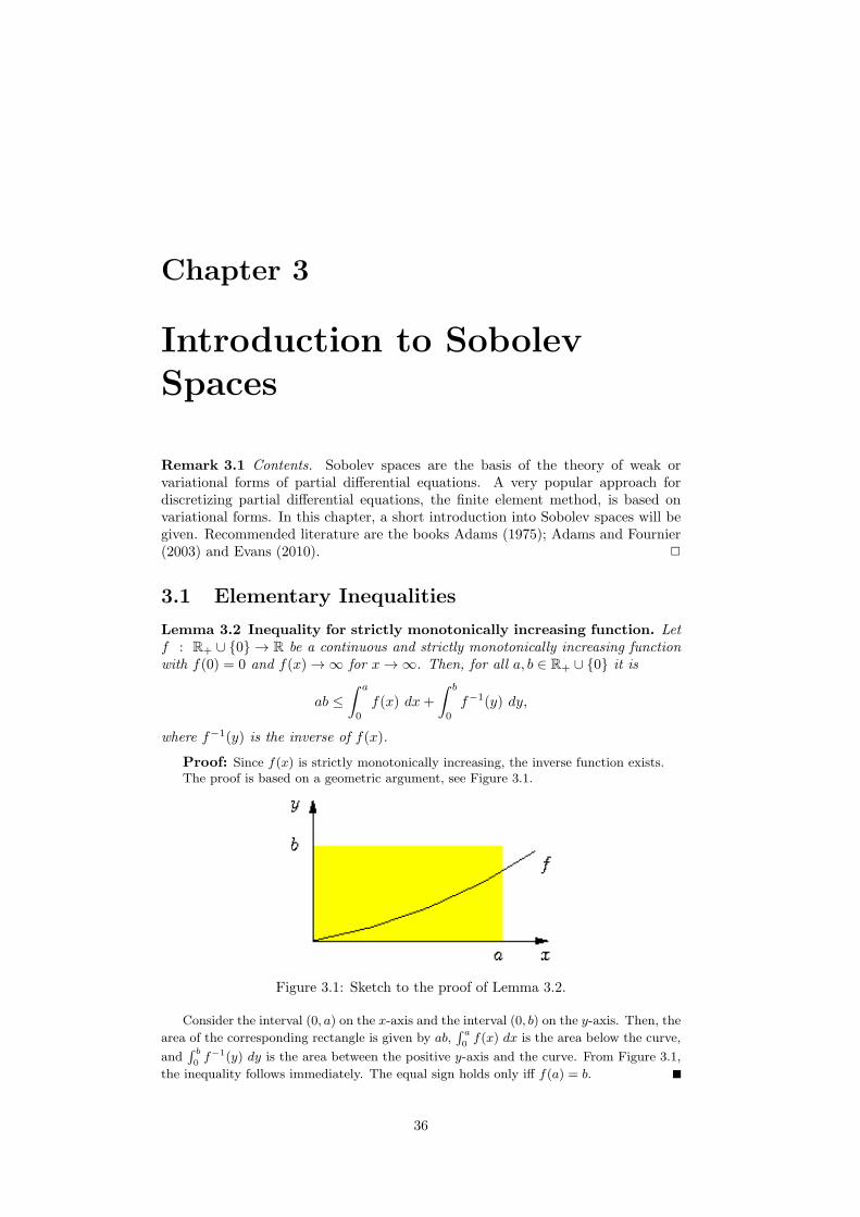
Proof: Since f(x) is strictly monotonically increasing, the inverse function exists.The proof is based on a geometric argument, see Figure 3.1.

Figure 3.1: Sketch to the proof of Lemma 3.2.

Consider the interval (0, a) on the x-axis and the interval (0, b) on the y-axis. Then, the

area of the corresponding rectangle is given by ab,∫ a

0f(x) dx is the area below the curve,

and∫ b

0f−1(y) dy is the area between the positive y-axis and the curve. From Figure 3.1,

the inequality follows immediately. The equal sign holds only iff f(a) = b.

36

Remark 3.3 Young’s inequality. Young’s inequality

ab ≤ε

2a2 +

1

2εb2 ∀ a, b, ε ∈ R+ (3.1)

follows from Lemma 3.2 with f(x) = εx, f−1(y) = ε−1y. It is also possible toderive this inequality from the binomial theorem. For proving the generalized Younginequality

ab ≤εp

pap +

1

qεqbq, ∀ a, b, ε ∈ R+ (3.2)

with p−1 + q−1 = 1, p, q ∈ (1,∞), one chooses f(x) = xp−1, f−1(y) = y1/(p−1) andapplies Lemma 3.2 with intervals where the upper bounds are given by εa and ε−1b.

Remark 3.4 Cauchy–Schwarz inequality. The Cauchy1–Schwarz2 inequality (forvectors, for sums)

|(x,y)| ≤ ‖x‖2 ‖y‖2 ∀ x,y ∈ Rn, (3.3)

where (·, ·) is the Euclidean product and ‖·‖2 the Euclidean norm, is well known.One can prove this inequality with the help of Young’s inequality.

First, it is clear that the Cauchy–Schwarz inequality is correct if one of thevectors is the zero vector. Now, let x,y with ‖x‖2 = ‖y‖2 = 1. One obtains withthe triangle inequality and Young’s inequality (3.1)

|(x,y)| =

∣∣∣∣∣

n∑

i=1

xiyi

∣∣∣∣∣≤

n∑

i=1

|xi| |yi| ≤1

2

n∑

i=1

|xi|2+

1

2

n∑

i=1

|yi|2= 1.

Hence, the Cauchy–Schwarz inequality is correct for x,y. Last, one considers arbi-trary vectors x 6= 0, y 6= 0. Now, one can utilize the homogeneity of the Cauchy–Schwarz inequality. From the validity of the Cauchy–Schwarz inequality for x andy, one obtains by a scaling argument

∣∣(‖x‖−1

2 x︸ ︷︷ ︸

x

, ‖y‖−12 y

︸ ︷︷ ︸

y

)∣∣ ≤ 1

Both vectors x,y have the Euclidean norm 1, hence

1

‖x‖2 ‖y‖2|(x, y)| ≤ 1 ⇐⇒ |(x, y)| ≤ ‖x‖2 ‖y‖2 .

The generalized Cauchy–Schwarz inequality or Holder inequality

|(x,y)| ≤

(n∑

i=1

|xi|p

)1/p( n∑

i=1

|yi|q

)1/q

with p−1 + q−1 = 1, p, q ∈ (1,∞), can be proved in the same way with the help ofthe generalized Young inequality.

Definition 3.5 Lebesgue spaces. The space of functions which are Lebesgueintegrable on Ω to the power of p ∈ [1,∞) is denoted by

Lp(Ω) =

f :

∫

Ω

|f |p(x) dx <∞

,

1Augustin Louis Cauchy (1789 – 1857)2Hermann Amandus Schwarz (1843 – 1921)

37

which is equipped with the norm

‖f‖Lp(x) =

(∫

Ω

|f |p(x) dx

)1/p

.

For p = ∞, this space is

L∞(Ω) = f : |f(x)| <∞ almost everywhere in Ω

with the norm‖f‖L∞(Ω) = ess supx∈Ω|f(x)|.

Lemma 3.6 Holder’s inequality. Let p−1 + q−1 = 1, p, q ∈ [1,∞]. If u ∈ Lp(Ω)and v ∈ Lq(Ω), then it is uv ∈ L1(Ω) and it holds that

‖uv‖L1(Ω) ≤ ‖u‖Lp(Ω) ‖v‖Lq(Ω) . (3.4)

If p = q = 2, then this inequality is also known as Cauchy–Schwarz inequality

‖uv‖L1(Ω) ≤ ‖u‖L2(Ω) ‖v‖L2(Ω) . (3.5)

Proof: p, q ∈ (1,∞). First, one has to show that |uv(x)| can be estimated fromabove by an integrable function. Setting in the generalized Young inequality (3.2) ε = 1,a = |u(x)|, and b = |v(x)| gives

|u(x)v(x)| ≤1

p|u(x)|p +

1

q|v(x)|q .

Since the right hand side of this inequality is integrable, by assumption, it follows thatuv ∈ L1(Ω). In addition, Holder’s inequality is proved for the case ‖u‖Lp(Ω) = ‖v‖Lq(Ω) = 1using this inequality

∫

Ω

|u(x)v(x)| dx ≤1

p

∫

Ω

|u(x)|p dx+1

q

∫

Ω

|v(x)|q dx = 1.

The general inequality follows, for the case that both functions do not vanish almosteverywhere, with the same homogeneity argument as used for proving the Cauchy–Schwarzinequality of sums. In the case that one of the functions vanishes almost everywhere, (3.4)is trivially satisfied.

p = 1, q = ∞. It is∫

Ω

|u(x)v(x)| dx ≤

∫

Ω

|u(x)| ess supx∈Ω|v(x)| dx = ‖u‖L1(Ω) ‖v‖L∞(Ω) .

3.2 Weak Derivative and Distributions

Remark 3.7 Contents. This section introduces a generalization of the derivativewhich is needed for the definition of weak or variational problems. For an introduc-tion to the topic of this section, see, e.g., Haroske and Triebel (2008)

Let Ω ⊂ Rd be a domain with boundary Γ = ∂Ω, d ∈ N, Ω 6= ∅. A domain is

always an open set.

Definition 3.8 The space C∞0 (Ω). The space of infinitely often differentiable real

functions with compact (closed and bounded) support in Ω is denoted by C∞0 (Ω)

C∞0 (Ω) = v : v ∈ C∞(Ω), supp(v) ⊂ Ω,

wheresupp(v) = x ∈ Ω : v(x) 6= 0.

38

Definition 3.9 Convergence in C∞0 (Ω). The sequence of functions φn(x)

∞n=1,

φn ∈ C∞0 (Ω) for all n, is said to convergence to the zero functions if and only if

a) ∃K ⊂ Ω,K compact (closed and bounded) with supp(φn) ⊂ K for all n,b) Dαφn(x) → 0 for n → ∞ on K for all multi-indices α = (α1, . . . , αd), |α| =

α1 + . . .+ αd.

It islimn→∞

φn(x) = φ(x) ⇐⇒ limn→∞

(φn(x)− φ(x)) = 0.

Definition 3.10 Weak derivative. Let f, F ∈ L1loc(Ω). (L1

loc(Ω): for each com-pact subset Ω′ ⊂ Ω it holds

∫

Ω′

|u(x)| dx <∞ ∀ u ∈ L1loc(Ω).)

If for all functions g ∈ C∞0 (Ω) it holds that

∫

Ω

F (x)g(x) dx = (−1)|α|

∫

Ω

f(x)Dαg(x) dx,

then F (x) is called weak derivative of f(x) with respect to the multi-index α.

Remark 3.11 On the weak derivative.

• One uses the same notations for the derivative as in the classical case : F (x) =Dαf(x).

• If f(x) is classically differentiable on Ω, then the classical derivative is also theweak derivative.

• The assumptions on f(x) and F (x) are such that the integrals in the definitionof the weak derivative are well defined. In particular, since the test functionsvanish in a neighborhood of the boundary, the behavior of f(x) and F (x) if xapproaches the boundary is not of importance.

• The main aspect of the weak derivative is due to the fact that the (Lebesgue)integral is not influenced from the values of the functions on a set of (Lebesgue)measure zero. Hence, the weak derivative is uniquely defined only up to a setof measure zero. It follows that f(x) might be not classically differentiable on aset of measure zero, e.g., in a point, but it can still be weakly differentiable.

• The weak derivative is uniquely determined, in the sense described above.

Example 3.12 Weak derivative. The weak derivative of the function f(x) = |x| is

f ′(x) =

−1 x < 00 x = 01 x > 0

In x = 0, one can use also any other real number. The proof of this statementfollows directly from the definition and it is left as an exercise.

Definition 3.13 Distribution. A continuous linear functional defined on C∞0 (Ω)

is called distribution. The set of all distributions is denoted by (C∞0 (Ω))

′.

Let u ∈ C∞0 (Ω) and ψ ∈ (C∞

0 (Ω))′, then the following notation is used for the

application of the distribution to the function

ψ(u(x)) = 〈ψ, u〉 ∈ R.

39

Remark 3.14 On distributions. Distributions are a generalization of functions.They assign each function from C∞

0 (Ω) a real number.

Example 3.15 Regular distribution. Let u(x) ∈ L1loc(Ω). Then, a distribution is

defined by ∫

Ω

u(x)φ(x) dx = 〈ψ, φ〉, ∀φ ∈ C∞0 (Ω).

This distribution will be identified with u(x) ∈ L1loc(Ω).

Distributions with such an integral representation are called regular, otherwisethey are called singular.

Example 3.16 Dirac distribution. Let ξ ∈ Ω fixed, then

〈δξ, φ〉 = φ(ξ) ∀ φ ∈ C∞0 (Ω)

defines a singular distribution, the so-called Dirac distribution or δ-distribution. Itis denoted by δξ = δ(x− ξ).

Definition 3.17 Derivatives of distributions. Let φ ∈ (C∞0 (Ω))

′be a distribution.

The distribution ψ ∈ (C∞0 (Ω))

′is called derivative in the sense of distributions or

distributional derivative of φ if

〈ψ, u〉 = (−1)|α|〈φ,Dαu〉 ∀u ∈ C∞0 (Ω),

α = (α1, . . . , αd), αj ≥ 0, j = 1, . . . , d, |α| = α1 + . . .+ αd.

Remark 3.18 On derivatives of distributions. Each distribution has derivatives inthe sense of distributions of arbitrary order.

If the derivative in the sense of distributions Dαu(x) of u(x) ∈ L1loc(Ω) is a

regular distribution, then also the weak derivative of u(x) exists and both derivativesare identified.

3.3 Lebesgue Spaces and Sobolev Spaces

Remark 3.19 On the spaces Lp(Ω). These spaces were introduced in Defini-tion 3.5.

• The elements of Lp(Ω) are, strictly speaking, equivalence classes of functionswhich are different only on a set of Lebesgue measure zero.

• The spaces Lp(Ω) are Banach spaces (complete normed spaces). A space X iscomplete, if each so-called Cauchy sequence un

∞n=0 ∈ X, i.e., for all ε > 0

there is an index n0(ε) such that for all i, j > n0(ε)

‖ui − uj‖X < ε.

converges and the limit is an element of X.• The space L2(Ω) becomes a Hilbert spaces with the inner product

(f, g) =

∫

Ω

f(x)g(x) dx, ‖f‖L2 = (f, f)1/2, f, g ∈ L2(Ω).

• The dual space of a space X is the space of all bounded linear functionals definedon X. Let Ω be a domain with sufficiently smooth boundary Γ. of the Lebesguespaces Lp(Ω), p ∈ [1,∞], then

(Lp(Ω))′

= Lq(Ω) with p, q ∈ (1,∞),1

p+

1

q= 1,

(L1(Ω)

)′= L∞(Ω),

(L∞(Ω))′ 6= L1(Ω).

40

The spaces L1(Ω), L∞(Ω) are not reflexive, i.e., the dual space of the dual spaceis not the original space again.

Definition 3.20 Sobolev3 spaces. Let k ∈ N ∪ 0 and p ∈ [1,∞], then theSobolev space W k,p(Ω) is defined by

W k,p(Ω) := u ∈ Lp(Ω) : Dαu ∈ Lp(Ω) ∀ α with |α| ≤ k.

This space is equipped with the norm

‖u‖Wk,p(Ω) :=∑

|α|≤k

‖Dαu‖Lp(Ω) . (3.6)

Remark 3.21 On the spaces W k,p(Ω).

• Definition 3.20 has the following meaning. From u ∈ Lp(Ω), p ∈ [1,∞), itfollows in particular that u ∈ L1

loc(Ω), such that u(x) defines (represents) adistribution. Then, all derivatives Dαu exist in the sense of distributions. Thestatement Dαu ∈ Lp(Ω) means that the distribution Dαu ∈ (C∞

0 (Ω))′can be

represented by a function from Lp(Ω).• One can add elements from W k,p(Ω) and one can multiply them with real num-bers. The result is again a function fromW k,p(Ω). With this property, the spaceW k,p(Ω) becomes a vector space (linear space). It is straightforward to checkthat (3.6) is a norm. (exercise)

• It is Dαu(x) = u(x) for α = (0, . . . , 0) and W 0,p(Ω) = Lp(Ω).• The spaces W k,p(Ω) are Banach spaces.• Sobolev spaces have for p ∈ [1,∞) a countable basis ϕn(x)

∞n=1 (Schauder

basis), i.e., each element u(x) can be written in the form

u(x) =

∞∑

n=1

unϕn(x), un ∈ R n = 1, . . . ,∞.

• Sobolev spaces are uniformly convex for p ∈ (1,∞), i.e., for each ε ∈ (0, 2] (notethat the largest distance in the ball is equal to 2) there is a δ(ε) > 0 such that forall u, v ∈ W k,p(Ω) with ‖u‖Wk,p(Ω) = ‖v‖Wk,p(Ω) = 1, and ‖u− v‖Wk,p(Ω) > ε

it holds that∥∥u+v

2

∥∥Wk,p(Ω)

≤ 1− δ(ε), see Figure 3.2 for an illustration.

• Sobolev spaces are reflexive for p ∈ (1,∞).• On can show that C∞(Ω) is dense inW k,p(Ω), e.g., see (Alt, 1999, Satz 1.21, Satz2.10) or (Adams, 1975, Lemma 3.15). With this property, one can characterizethe Sobolev spaces W k,p(Ω) as completion of the functions from C∞(Ω) withrespect to the norm (3.6). For domains with smooth boundary, one can evenshow that C∞(Ω) is dense in W k,p(Ω).

• The Sobolev space Hk(Ω) =W k,2(Ω) is a Hilbert space with the inner product

(u, v)Hk(Ω) =∑

|α|≤k

∫

Ω

Dαu(x)Dαv(x) dx

and the norm ‖u‖Hk(Ω) = (u, u)1/2.

3Sergei Lvovich Sobolev (1908 – 1989)

41

Figure 3.2: Illustration of the uniform convexity of Sobolev spaces.

Definition 3.22 The space W k,p0 (Ω). The Sobolev space W k,p

0 (Ω) is defined asthe completion of C∞

0 (Ω) in the norm of W k,p(Ω)

W k,p0 (Ω) = C∞

0 (Ω)‖·‖

Wk,p(Ω) .

3.4 The Trace of a Function from a Sobolev Space

Remark 3.23 Motivation. This class considers boundary value problems for par-tial differential equations. In the theory of weak or variational solutions, the solu-tion of the partial differential equation is searched in an appropriate Sobolev space.Then, for the boundary value problem, this solution has to satisfy the boundarycondition. However, since the boundary of a domain is a manifold of dimension(d − 1), and consequently it has Lebesgue measure zero, one has to clarify how afunction from a Sobolev space is defined on this manifold. This definition will bepresented in this section.

Definition 3.24 Boundary of class Ck,α. A bounded domain Ω ⊂ Rd and its

boundary Γ are of class Ck,α, 0 ≤ α ≤ 1 if for all x0 ∈ Γ there is a ball B(x0, r)with r > 0 and a bijective map ψ : B(x0, r) → D ⊂ R

d such that

1) ψ (B(x0, r) ∩ Ω) ⊂ Rd+,

2) ψ (B(x0, r) ∩ Γ) ⊂ ∂Rd+,

3) ψ ∈ Ck,α(B(x0, r)), ψ−1 ∈ Ck,α(D), are Holder continuous.

That means, Γ is locally the graph of a function with d− 1 arguments. (A functionu(x) is Holder continuous if

‖u‖Ck,α(Ω) =∑

|α|≤k

‖Dαu‖C(Ω) +∑

|α|=k

[Dαu]C0,α(Ω)

with

[Dαu]C0,α(Ω) = supx,y∈Ω

|u(x)− u(y)|

|x− y|α

is finite.)

Remark 3.25 Lipschitz boundary. It will be generally assumed that the boundaryof Ω is of class C0,1. That means, the map is Lipschitz4 continuous. Such a boundary

4Rudolf Otto Sigismund Lipschitz (1832 – 1903)

42

is simply called Lipschitz boundary and the domain is called Lipschitz domain. Animportant feature of a Lipschitz boundary is that the outer normal vector is definedalmost everywhere at the boundary and it is almost everywhere continuous.

Example 3.26 On Lipschitz domains.

• Domains with Lipschitz boundary are, for example, balls or polygonal domainsin two dimensions where the domain is always on one side of the boundary.

• A domain which is not a Lipschitz domain is a circle with a slit

Ω = (x, y) : x2 + y2 < 1 \ (x, y) : x ≥ 0, y = 0.

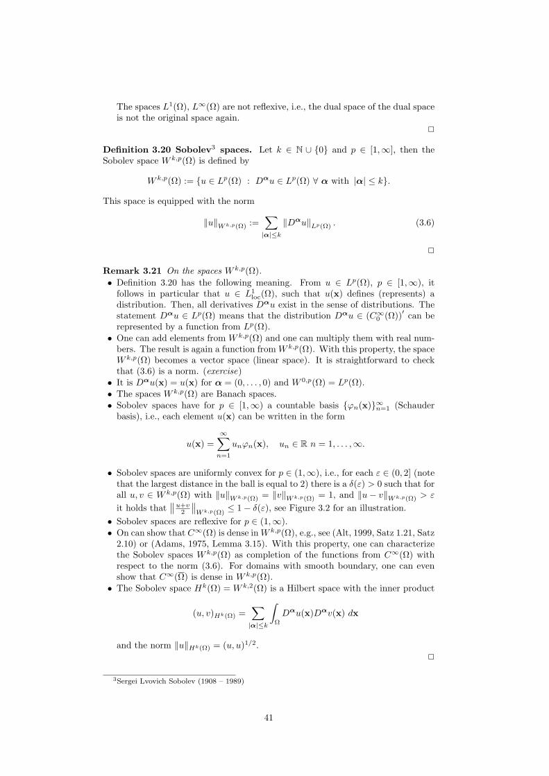
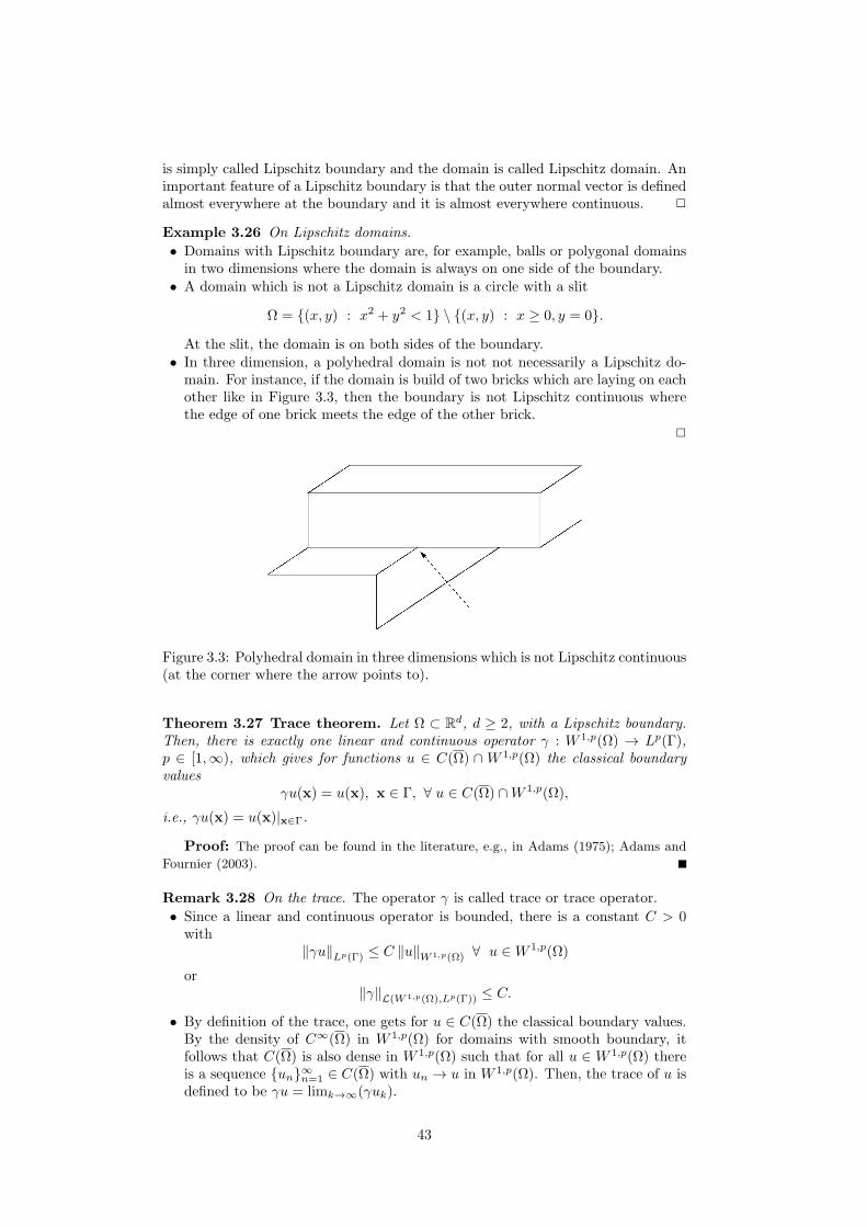
At the slit, the domain is on both sides of the boundary.• In three dimension, a polyhedral domain is not not necessarily a Lipschitz do-main. For instance, if the domain is build of two bricks which are laying on eachother like in Figure 3.3, then the boundary is not Lipschitz continuous wherethe edge of one brick meets the edge of the other brick.

Figure 3.3: Polyhedral domain in three dimensions which is not Lipschitz continuous(at the corner where the arrow points to).

Theorem 3.27 Trace theorem. Let Ω ⊂ Rd, d ≥ 2, with a Lipschitz boundary.

Then, there is exactly one linear and continuous operator γ : W 1,p(Ω) → Lp(Γ),p ∈ [1,∞), which gives for functions u ∈ C(Ω) ∩W 1,p(Ω) the classical boundaryvalues

γu(x) = u(x), x ∈ Γ, ∀ u ∈ C(Ω) ∩W 1,p(Ω),

i.e., γu(x) = u(x)|x∈Γ.

Proof: The proof can be found in the literature, e.g., in Adams (1975); Adams and

Fournier (2003).

Remark 3.28 On the trace. The operator γ is called trace or trace operator.

• Since a linear and continuous operator is bounded, there is a constant C > 0with

‖γu‖Lp(Γ) ≤ C ‖u‖W 1,p(Ω) ∀ u ∈W 1,p(Ω)

or‖γ‖L(W 1,p(Ω),Lp(Γ)) ≤ C.

• By definition of the trace, one gets for u ∈ C(Ω) the classical boundary values.By the density of C∞(Ω) in W 1,p(Ω) for domains with smooth boundary, itfollows that C(Ω) is also dense in W 1,p(Ω) such that for all u ∈ W 1,p(Ω) thereis a sequence un

∞n=1 ∈ C(Ω) with un → u in W 1,p(Ω). Then, the trace of u is

defined to be γu = limk→∞(γuk).

43

• It is

γu(x) = 0 ∀ u ∈W 1,p0 (Ω),

γDαu(x) = 0 ∀ u ∈W k,p0 (Ω), |α| ≤ k − 1. (3.7)

3.5 Sobolev Spaces with Non-Integer and Nega-

tive Exponents

Remark 3.29 Motivation. Sobolev spaces with non-integer and negative expo-nents are important in the theory of variational formulations of partial differentialequations.

Let Ω ⊂ Rd be a domain and p ∈ (1,∞) mit p−1 + q−1 = 1.

Definition 3.30 The space W−k,q(Ω). The space W−k,q(Ω), k ∈ N ∪ 0, con-tains distributions which are defined on W k,p(Ω)

W−k,q(Ω) =ϕ ∈ (C∞

0 (Ω))′: ‖ϕ‖W−k,q <∞

with

‖ϕ‖W−k,q = supu∈C∞

0 (Ω),u 6=0

〈ϕ, u〉

‖u‖Wk,p(Ω)

.

Remark 3.31 On the spaces W−k,p(Ω).

• It is W−k,q(Ω) =[

W k,p0 (Ω)

]′

, i.e., W−k,q(Ω) can be identified with the dual

space of W k,p0 (Ω). In particular it is H−1(Ω) =

(H1

0 (Ω))′.

• It is

. . . ⊂W 2,p(Ω) ⊂W 1,p(Ω) ⊂ Lp(Ω) ⊂W−1,q(Ω) ⊂W−2,q(Ω) . . .

Definition 3.32 Sobolev–Slobodeckij space. Let s ∈ R, then the Sobolev–Slobodeckij or Sobolev space Hs(Ω) is defined as follows:

• s ∈ Z. Hs(Ω) =W s,2(Ω).• s > 0 with s = k + σ, k ∈ N ∪ 0, σ ∈ (0, 1). The space Hs(Ω) contains allfunctions u for which the following norm is finite:

‖u‖2Hs(Ω) = ‖u‖2Hk(Ω) + |u|2k+σ ,

with

(u, v)Hs(Ω) = (u, v)Hk + (u, v)k+σ, |u|2k+σ = (u, u)k+σ,

(u, v)k+σ =∑

|α|=k

∫

Ω

∫

Ω

(Dαu(x)−Dαu(y)) (Dαv(x)−Dαv(y))

‖x− y‖d+2σ2

dxdy,

• s < 0. Hs(Ω) =[H−s

0 (Ω)]′

with H−s0 (Ω) = C∞

0 (Ω)‖·‖H−s(Ω) .

44

3.6 Theorem on Equivalent Norms

Definition 3.33 Equivalent norms. Two norms ‖·‖1 and ‖·‖2 on the linear spaceX are said to be equivalent if there are constants C1 and C2 such that

C1 ‖u‖1 ≤ ‖u‖2 ≤ C2 ‖u‖1 ∀ u ∈ X.

Remark 3.34 On equivalent norms. Many important properties, like continuityor convergence, do not change if an equivalent norm is considered.

Theorem 3.35 Equivalent norms in W k,p(Ω). Let Ω ⊂ Rd be a domain with

Lipschitz boundary Γ, p ∈ [1,∞], and k ∈ N. Let fili=1 be a system with the

following properties:

1) fi : W k,p(Ω) → R+ ∪ 0 is a semi norm,2) ∃Ci > 0 with 0 ≤ fi(v) ≤ Ci ‖v‖Wk,p(Ω), ∀ v ∈W k,p(Ω),

3) fi is a norm on the polynomials of degree k − 1, i.e., if for v ∈ Pk−1 =∑

|α|≤k−1 Cαxα

it holds that fi(v) = 0, i = 1, . . . , l, then it is v ≡ 0.

Then, the norm ‖·‖Wk,p(Ω) defined in (3.6) and the norm

‖u‖′Wk,p(Ω) :=

(l∑

i=1

fpi (u) + |u|pWk,p(Ω)

)1/p

with

|u|Wk,p(Ω) =

∑

|α|=k

∫

Ω

|Dαu(x)|p dx

1/p

are equivalent.

Remark 3.36 On semi norms. For a semi norm fi(·), one cannot conclude fromfi(v) = 0 that v = 0. The third assumptions however states, that this conclusioncan be drawn for all polynomials up to a certain degree.

Example 3.37 Equivalent norms in Sobolev spaces.

• The following norms are equivalent to the standard norm in W 1,p(Ω):

a) ‖u‖′W 1,p(Ω) =

(∣∣∣∣

∫

Ω

u dx

∣∣∣∣

p

+ |u|pW 1,p(Ω)

)1/p

,

b) ‖u‖′W 1,p(Ω) =

(∣∣∣∣

∫

Γ

u ds

∣∣∣∣

p

+ |u|pW 1,p(Ω)

)1/p

,

c) ‖u‖′W 1,p(Ω) =

(∫

Γ

|u|p ds+ |u|pW 1,p(Ω)

)1/p

.

• In W k,p(Ω) it is

‖u‖′Wk,p(Ω) =

(k−1∑

i=0

∫

Γ

∣∣∣∣

∂iu

∂ni

∣∣∣∣

p

ds+ |u|pWk,p(Ω)

)1/p

equivalent to the standard norm. Here, n denotes the outer normal on Γ with‖n‖2 = 1.

45

• In the case W k,p0 (Ω), one does not need the regularity of the boundary. It is

‖u‖′Wk,p0 (Ω) = |u|Wk,p(Ω) ,

i.e., in the spaces W k,p0 (Ω) the standard semi norm is equivalent to the standard

norm.In particular, it is for u ∈ H1

0 (Ω) (k = 1, p = 2)

C1 ‖u‖H1(Ω) ≤ ‖∇u‖L2(Ω) ≤ C2 ‖u‖H1(Ω) .

It follows that there is a constant C > 0 such that

‖u‖L2(Ω) ≤ C ‖∇u‖L2(Ω) ∀ u ∈ H10 (Ω). (3.8)

3.7 Some Inequalities in Sobolev Spaces

Remark 3.38 Motivation. This section presents a generalization of the last part ofExample 3.37. It will be shown that for inequalities of type (3.8) it is not necessarythat the trace vanishes on the complete boundary.

Let Ω ⊂ Rd be a bounded domain with boundary Γ and let Γ1 ⊂ Γ with

measRd−1 (Γ1) =∫

Γ1ds > 0.

One considers the space

V0 =v ∈W 1,p(Ω) : v|Γ1 = 0

⊂W 1,p(Ω) if Γ1 ⊂ Γ,

V0 = W 1,p0 (Ω) if Γ1 = Γ

with p ∈ [1,∞).

Lemma 3.39 Friedrichs5 inequality, Poincare6 inequality, Poincare–Fried-

richs inequality. Let p ∈ [1,∞) and measRd−1 (Γ1) > 0. Then it is for all u ∈ V0∫

Ω

|u(x)|p dx ≤ CP

∫

Ω

‖∇u(x)‖p2 dx, (3.9)

where ‖·‖2 is the Euclidean vector norm.

Proof: The inequality will be proved with the theorem on equivalent norms, Theo-rem 3.35. Let f1(u) : W 1,p(Ω) → R+ ∪ 0 with

f1(u) =

(∫

Γ1

|u(s)|p ds

)1/p

.

This functions has the following properties:

1) f1(u) is a semi norm.

2) It is

0 ≤ f1(u) =

(∫

Γ1

|u(s)|p ds

)1/p

≤

(∫

Γ

|u(s)|p ds

)1/p

= ‖u‖Lp(Γ) = ‖γu‖Lp(Γ) ≤ C ‖u‖W1,p(Ω) .

The last estimate follows from the continuity of the trace operator.

5Friedrichs6Poincare

46

3) Let v ∈ P0, i.e., v is a constant. Then, one obtains from

0 = f1(v) =

(∫

Γ1

|v(s)|p ds

)1/p

= |v| (measRd−1 (Γ1))1/p ,

that |v| = 0.

Hence, all assumptions of Theorem 3.35 are satisfied. That means, there are two constantsC1 and C2with

C1

(∫

Γ1

|u(s)|p ds+

∫

Ω

‖∇u(x)‖p2 dx

)1/p

︸ ︷︷ ︸

‖u‖′W1,p(Ω)

≤ ‖u‖W1,p(Ω) ≤ C2 ‖u‖′W1,p(Ω) ∀ u ∈ W 1,p(Ω).

In particular, it follows that

∫

Ω

|u(x)|p dx+

∫

Ω

‖∇u(x)‖p2 dx ≤ Cp2

(∫

Γ1

|u(s)|p ds+

∫

Ω

‖∇u(x)‖p2 dx

)

or ∫

Ω

|u(x)|p dx ≤ CP

(∫

Γ1

|u(s)|p ds+

∫

Ω

‖∇u(x)‖p2 dx

)

with CP = Cp2 . Since u ∈ V0 vanishes on Γ1, the statement of the lemma is proved.

Remark 3.40 On the Poincare–Friedrichs inequality. In the space V0 becomes|·|W 1,p a norm which is equivalent to ‖·‖W 1,p(Ω). The classical Poincare–Friedrichsinequality is given for Γ1 = Γ and p = 2

‖u‖L2 ≤ CP ‖∇u‖L2 ∀ u ∈ H10 (Ω),

where the constant depends only on the diameter of the domain Ω.

Lemma 3.41 Another inequality of Poincare–Friedrichs type. Let Ω′ ⊂ Ωwith measRd (Ω′) =

∫

Ω′dx > 0, then for all u ∈W 1,p(Ω) it is

∫

Ω

|u(x)|p dx ≤ C

(∣∣∣∣

∫

Ω′

u(x) dx

∣∣∣∣

p

+

∫

Ω

‖∇u(x)‖p2 dx

)

.

Proof: Exercise.

3.8 The Gaussian Theorem

Remark 3.42 Motivation. The Gaussian theorem is the generalization of the in-tegration by parts from calculus. This operation is very important for the theoryof weak or variational solutions of partial differential equations. One has to study,under which conditions on the regularity of the domain and of the functions it iswell defined.

Theorem 3.43 Gaussian theorem. Let Ω ⊂ Rd, d ≥ 2, be a bounded domain

with Lipschitz boundary Γ. Then, the following identity holds for all u ∈W 1,1(Ω)

∫

Ω

∂iu(x) dx =

∫

Γ

u(s)ni(s) ds, (3.10)

where n is the unit outer normal vector on Γ.

47

Proof: sketch. First of all, one proves the statement for functions from C1(Ω). Thisproof is somewhat longer and it is referred to the literature, e.g., Evans (2010).

The space C1(Ω) is dense in W 1,1(Ω), see Remark 3.21. Hence, for all u ∈ W 1,1(Ω)there is a sequence un

∞n=1 ∈ C1(Ω) with

limn→∞

‖u− un‖W1,1(Ω) = 0

and (3.10) holds for all functions un(x). It will be shown that the limit of the left handside converges to the left hand side of (3.10) and the limit of the right hand side convergesto the right hand side of (3.10).

From the convergence in ‖·‖W1,1(Ω), one has in particular

limn→∞

∫

Ω

∂iun(x) dx =

∫

Ω

∂iu(x) dx.

On the other hand, the continuity of the trace operator gives

limn→∞

‖u− un‖L1(Γ) ≤ C limn→∞

‖u− un‖W1,1 = 0,

from what follows that

limn→∞

∫

Γ

un(s) ds =

∫

Γ

u(s) ds.

Since for a Lipschitz boundary, the normal n is almost everywhere continuous, it is

limn→∞

∫

Γ

un(s)ni(s) ds =

∫

Γ

u(s)ni(s) ds.

Thus, the limits lead to (3.10).

Corollary 3.44 Vector field. Let the conditions of Theorem 3.43 on the domain

Ω be satisfied and let u ∈(W 1,1(Ω)

)dbe a vector field. Then it is

∫

Ω

∇ · u(x) dx =

∫

Γ

u(s) · n(s) ds.

Proof: The statement follows by adding (3.10) from i = 1 to i = d.

Corollary 3.45 Integration by parts. Let the conditions of Theorem 3.43 onthe domain Ω be satisfied. Consider u ∈W 1,p(Ω) and v ∈W 1,q(Ω) with p ∈ (1,∞)and 1

p + 1q = 1. Then it is

∫

Ω

∂iu(x)v(x) dx =

∫

Γ

u(s)v(s)ni(s) ds−

∫

Ω

u(x)∂iv(x) dx.

Proof: exercise.

Corollary 3.46 First Green7’s formula. Let the conditions of Theorem 3.43 onthe domain Ω be satisfied, then it is

∫

Ω

∇u(x) · ∇v(x) dx =

∫

Γ

∂u

∂n(s)v(s) ds−

∫

Ω

∆u(x)v(x) dx

for all u ∈ H2(Ω) and v ∈ H1(Ω).

Proof: From the definition of the Sobolev spaces it follows that the integrals are well

defined. Now, the proof follows the proof of Corollary 3.45, where one has now to sum

over the components.

7Georg Green (1793 – 1841)

48

Remark 3.47 On the first Green’s formula. The first Green’s formula is the for-mula of integrating by parts once. The boundary integral can be equivalently writ-ten in the form ∫

Γ

∇u(s) · n(s)v(s) ds.

The formula of integrating by parts twice is called second Green’s formula.

Corollary 3.48 Second Green’s formula. Let the conditions of Theorem 3.43on the domain Ω be satisfied, then one has

∫

Ω

(∆u(x)v(x)−∆v(x)u(x)

)dx =

∫

Γ

(∂u

∂n(s)v(s)−

∂v

∂n(s)u(s)

)

ds

for all u, v ∈ H2(Ω).

3.9 Sobolev Imbedding Theorems

Remark 3.49 Motivation. This section studies the question which Sobolev spacesare subspaces of other Sobolev spaces. With this property, called imbedding, it ispossible to estimate the norm of a function in the subspace by the norm in thelarger space.

Lemma 3.50 Imbedding of Sobolev spaces with same integration power pand different orders of the derivative. Let Ω ⊂ R

d be a domain with p ∈ [1,∞)and k ≤ m, then it is Wm,p(Ω) ⊂W k,p(Ω).

Proof: The statement of this lemma follows directly from the definition of Sobolev

spaces, see Definition 3.20.

Lemma 3.51 Imbedding of Sobolev spaces with the same order of the

derivative k and different integration powers. Let Ω ⊂ Rd be a bounded

domain, k ≥ 0, and p, q ∈ [1,∞] with q > p. Then it is W k,q(Ω) ⊂W k,p(Ω).

Proof: exercise.

Remark 3.52 Imbedding of Sobolev spaces with the same order of the derivative kand the same integration power p in imbedded domains. Let Ω ⊂ R

d be a domainwith sufficiently smooth boundary Γ, k ≥ 0, and p ∈ [1,∞]. Then there is a mapE : W k,p(Ω) →W k,p(Rd), the so-called (simple) extension, with

• Ev|Ω = v,• ‖Ev‖Wk,p(Rd) ≤ C ‖v‖Wk,p(Ω), with C > 0,

e.g., see (Adams, 1975, Chapter IV) for details. Likewise, the natural restrictione : W k,p(Rd) →W k,p(Ω) can be defined and it is ‖ev‖Wk,p(Ω) ≤ ‖v‖Wk,p(Rd).

Theorem 3.53 A Sobolev inequality. Let Ω ⊂ Rd be a bounded domain with

Lipschitz boundary Γ, k ≥ 0, and p ∈ [1,∞) with

k ≥ d for p = 1,k > d/p for p > 1.

Then there is a constant C such that for all u ∈W k,p(Ω) it follows that u ∈ CB(Ω),where

CB(Ω) = v ∈ C(Ω) : v is bounded ,

and it is‖u‖CB(Ω) = ‖u‖L∞(Ω) ≤ C ‖u‖Wk,p(Ω) . (3.11)

49

Proof: See literature, e.g., Adams (1975); Adams and Fournier (2003).

Remark 3.54 On the Sobolev inequality. The Sobolev inequality states that eachfunction with sufficiently many weak derivatives (the number depends on the di-mension of Ω and the integration power) can be considered as a continuous andbounded function in Ω. One says that W k,p(Ω) is imbedded in CB(Ω). It is

C(Ω)⊂ CB(Ω) ⊂ C(Ω).

Consider Ω = (0, 1) and f1(x) = 1/x and f2(x) = sin(1/x). Then, f1 ∈ C(Ω),f1 6∈ CB(Ω) and f2 ∈ CB(Ω), f2 6∈ C(Ω).

Of course, it is possible to apply this theorem to weak derivatives of functions.Then, one obtains imbeddings like W k,p(Ω) → Cs

B(Ω) for (k − s)p > d, p > 1. Acomprehensive overview on imbeddings can be found in Adams (1975); Adams andFournier (2003).

Example 3.55 H1(Ω) in one dimension. Let d = 1 and Ω be a bounded interval.Then, each function from H1(Ω) (k = 1, p = 2) is continuous and bounded in Ω.

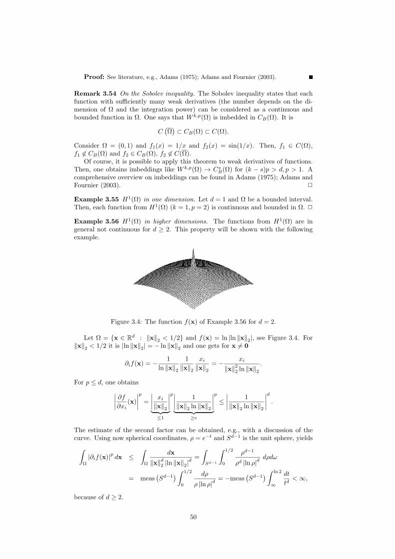
Example 3.56 H1(Ω) in higher dimensions. The functions from H1(Ω) are ingeneral not continuous for d ≥ 2. This property will be shown with the followingexample.

Figure 3.4: The function f(x) of Example 3.56 for d = 2.

Let Ω = x ∈ Rd : ‖x‖2 < 1/2 and f(x) = ln |ln ‖x‖2|, see Figure 3.4. For

‖x‖2 < 1/2 it is |ln ‖x‖2| = − ln ‖x‖2 and one gets for x 6= 0

∂if(x) = −1

ln ‖x‖2

1

‖x‖2

xi‖x‖2

= −xi

‖x‖22 ln ‖x‖2.

For p ≤ d, one obtains

∣∣∣∣

∂f

∂xi(x)

∣∣∣∣

p

=

∣∣∣∣

xi‖x‖2

∣∣∣∣

︸ ︷︷ ︸

≤1

p∣∣∣∣

1

‖x‖2 ln ‖x‖2

∣∣∣∣

︸ ︷︷ ︸

≥e

p

≤

∣∣∣∣

1

‖x‖2 ln ‖x‖2

∣∣∣∣

d

.

The estimate of the second factor can be obtained, e.g., with a discussion of thecurve. Using now spherical coordinates, ρ = e−t and Sd−1 is the unit sphere, yields

∫

Ω

|∂if(x)|pdx ≤

∫

Ω

dx

‖x‖d2 |ln ‖x‖2|d=

∫

Sd−1

∫ 1/2

0

ρd−1

ρd |ln ρ|ddρdω

= meas(Sd−1

)∫ 1/2

0

dρ

ρ |ln ρ|d= −meas

(Sd−1

)∫ ln 2

∞

dt

td<∞,

because of d ≥ 2.

50

It follows that ∂if ∈ Lp(Ω) with p ≤ d. Analogously, one proves that f ∈ Lp(Ω)with p ≤ d. Altogether, one has f ∈W 1,p(Ω) with p ≤ d. However, it is f 6∈ L∞(Ω).This example shows that the condition k > d/p for p > 1 is sharp.

In particular, it was proved for p = 2 that from f ∈ H1(Ω) in general it doesnot follow that f ∈ C(Ω).

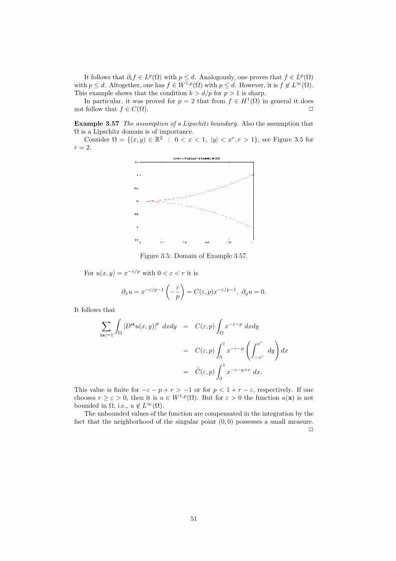
Example 3.57 The assumption of a Lipschitz boundary. Also the assumption thatΩ is a Lipschitz domain is of importance.

Consider Ω = (x, y) ∈ R2 : 0 < x < 1, |y| < xr, r > 1, see Figure 3.5 for

r = 2.

Figure 3.5: Domain of Example 3.57.

For u(x, y) = x−ε/p with 0 < ε < r it is

∂xu = x−ε/p−1

(

−ε

p

)

= C(ε, p)x−ε/p−1, ∂yu = 0.

It follows that

∑

|α|=1

∫

Ω

|Dαu(x, y)|p dxdy = C(ε, p)

∫

Ω

x−ε−p dxdy

= C(ε, p)

∫ 1

0

x−ε−p

(∫ xr

−xr

dy

)

dx

= C(ε, p)

∫ 1

0

x−ε−p+r dx.

This value is finite for −ε − p + r > −1 or for p < 1 + r − ε, respectively. If onechooses r ≥ ε > 0, then it is u ∈ W 1,p(Ω). But for ε > 0 the function u(x) is notbounded in Ω, i.e., u 6∈ L∞(Ω).

The unbounded values of the function are compensated in the integration by thefact that the neighborhood of the singular point (0, 0) possesses a small measure.

51

Chapter 4

The Ritz Method and the

Galerkin Method

Remark 4.1 Contents. This chapter studies variational or weak formulations ofboundary value problems of partial differential equations in Hilbert spaces. Theexistence and uniqueness of an appropriately defined weak solution will be discussed.The approximation of this solution with the help of finite-dimensional spaces iscalled Ritz method or Galerkin method. Some basic properties of this method willbe proved.

In this chapter, a Hilbert space V will be considered with inner product a(·, ·) :V × V → R and norm ‖v‖V = a(v, v)1/2.

4.1 The Theorems of Riesz and Lax–Milgram

Theorem 4.2 Representation theorem of Riesz. Let f ∈ V ′ be a continuousand linear functional, then there is a uniquely determined u ∈ V with

a(u, v) = f(v) ∀ v ∈ V. (4.1)

In addition, u is the unique solution of the variational problem

F (v) =1

2a(v, v)− f(v) → min ∀ v ∈ V. (4.2)

Proof: First, the existence of a solution u of the variational problem will be proved.Since f is continuous, it holds

|f(v)| ≤ c ‖v‖V ∀ v ∈ V,

from what follows that

F (v) ≥1

2‖v‖2V − c ‖v‖V ≥ −

1

2c2,

where in the last estimate the necessary criterion for a local minimum of the expression ofthe first estimate is used. Hence, the function F (·) is bounded from below and

d = infv∈V

F (v)

exists.Let vkk∈N be a sequence with F (vk) → d for k → ∞. A straightforward calculation

(parallelogram identity in Hilbert spaces) gives

‖vk − vl‖2V + ‖vk + vl‖

2V = 2 ‖vk‖

2V + 2 ‖vl‖

2V .

52

Using the linearity of f(·) and d ≤ F (v) for all v ∈ V , one obtains

‖vk − vl‖2V

= 2 ‖vk‖2V + 2 ‖vl‖

2V − 4

∥∥∥vk + vl

2

∥∥∥

2

V− 4f(vk)− 4f(vl) + 8f

(vk + vl2

)

= 4F (vk) + 4F (vl)− 8F(vk + vl

2

)

≤ 4F (vk) + 4F (vl)− 8d → 0

for k, l → ∞. Hence vkk∈N is a Cauchy sequence. Because V is a complete space, thereexists a limit u of this sequence with u ∈ V . Because F (·) is continuous, it is F (u) = dand u is a solution of the variational problem.

In the next step, it will be shown that each solution of the variational problem (4.2)is also a solution of (4.1). It is

Φ(ε) = F (u+ εv) =1

2a(u+ εv, u+ εv)− f(u+ εv)

=1

2a(u, u) + εa(u, v) +

ε2

2a(v, v)− f(u)− εf(v).

If u is a minimum of the variational problem, then the function Φ(ε) has a local minimumat ε = 0. The necessary condition for a local minimum leads to

0 = Φ′(0) = a(u, v)− f(v) for all v ∈ V.

Finally, the uniqueness of the solution will be proved. It is sufficient to prove theuniqueness of the solution of the equation (4.1). If the solution of (4.1) is unique, thenthe existence of two solutions of the variational problem (4.2) would be a contradiction tothe fact proved in the previous step. Let u1 and u2 be two solutions of the equation (4.1).Computing the difference of both equations gives

a(u1 − u2, v) = 0 for all v ∈ V.

This equation holds, in particular, for v = u1 − u2. Hence, ‖u1 − u2‖V = 0, such that

u1 = u2.

Definition 4.3 Bounded bilinear form, coercive bilinear form, V -elliptic

bilinear form. Let b(·, ·) : V × V → R be a bilinear form on the Banach spaceV . Then it is bounded if

|b(u, v)| ≤M ‖u‖V ‖v‖V ∀ u, v ∈ V,M > 0, (4.3)

where the constant M is independent of u and v. The bilinear form is coercive orV -elliptic if

b(u, u) ≥ m ‖u‖2V ∀ u ∈ V,m > 0, (4.4)

where the constant m is independent of u.

Remark 4.4 Application to an inner product. Let V be a Hilbert space. Then theinner product a(·, ·) is a bounded and coercive bilinear form, since by the Cauchy–Schwarz inequality

|a(u, v)| ≤ ‖u‖V ‖v‖V ∀ u, v ∈ V,

and obviously a(u, u) = ‖u‖2V . Hence, the constants can be chosen to be M = 1and m = 1.

Next, the representation theorem of Riesz will be generalized to the case ofcoercive and bounded bilinear forms.

Theorem 4.5 Theorem of Lax–Milgram. Let b(·, ·) : V × V → R be abounded and coercive bilinear form on the Hilbert space V . Then, for each boundedlinear functional f ∈ V ′ there is exactly one u ∈ V with

b(u, v) = f(v) ∀ v ∈ V. (4.5)

53

Proof: One defines linear operators T, T ′ : V → V by

a(Tu, v) = b(u, v) ∀ v ∈ V, a(T ′u, v) = b(v, u) ∀ v ∈ V. (4.6)

Since b(u, ·) and b(·, u) are continuous linear functionals on V , it follows from Theorem 4.2that the elements Tu and T ′u exist and they are defined uniquely. Because the operatorssatisfy the relation

a(Tu, v) = b(u, v) = a(T ′v, u) = a(u, T ′v), (4.7)

T ′ is called adjoint operator of T . Setting v = Tu in (4.6) and using the boundedness ofb(·, ·) yields

‖Tu‖2V = a(Tu, Tu) = b(u, Tu) ≤ M ‖u‖V ‖Tu‖V =⇒ ‖Tu‖V ≤ M ‖u‖V

for all u ∈ V . Hence, T is bounded. Since T is linear, it follows that T is continuous.Using the same argument, one shows that T ′ is also bounded and continuous.

Define the bilinear form

d(u, v) := a(TT ′u, v) = a(T ′u, T ′v) ∀ u, v ∈ V,

where (4.7) was used. Hence, this bilinear form is symmetric. Using the coercivity of b(·, ·)and the Cauchy–Schwarz inequality gives

m2 ‖v‖4V ≤ b(v, v)2 = a(T ′v, v)2 ≤ ‖v‖2V∥∥T ′v

∥∥2

V= ‖v‖2V a(T ′v, T ′v) = ‖v‖2V d(v, v).

Applying now the boundedness of a(·, ·) and of T ′ yields

m2 ‖v‖2V ≤ d(v, v) = a(T ′v, T ′v) =∥∥T ′v

∥∥2

V≤ M ‖v‖2V . (4.8)

Hence, d(·, ·) is also coercive and, since it is symmetric, it defines an inner product on V .From (4.8) one has that the norm induced by d(v, v)1/2 is equivalent to the norm ‖v‖V .From Theorem 4.2 it follows that there is a exactly one w ∈ V with

d(w, v) = f(v) ∀ v ∈ V.

Inserting u = T ′w into (4.5) gives with (4.6)

b(T ′w, v) = a(TT ′w, v) = d(w, v) = f(v) ∀ v ∈ V,

hence u = T ′w is a solution of (4.5).

The uniqueness of the solution is proved analogously as in the symmetric case.

4.2 Weak Formulation of Boundary Value Prob-

lems

Remark 4.6 Model problem. Consider the Poisson equation with homogeneousDirichlet boundary conditions

−∆u = f in Ω ⊂ Rd,

u = 0 on ∂Ω.(4.9)

Definition 4.7 Weak formulation of (4.9). Let f ∈ L2(Ω). A weak formulationof (4.9) consists in finding u ∈ V = H1

0 (Ω) such that

a(u, v) = (f, v) ∀ v ∈ V (4.10)

with

a(u, v) = (∇u,∇v) =

∫

Ω

∇u(x) · ∇v(x) dx

and (·, ·) is the inner product in L2(Ω).

54

Remark 4.8 On the weak formulation.

• The weak formulation is also called variational formulation.• As usual in mathematics, ’weak’ means that something holds for all appropri-ately chosen test functions.

• Formally, one obtains the weak formulation by multiplying the strong form ofthe equation (4.9) with the test function, by integrating the equation on Ω, andapplying integration by parts. Because of the Dirichlet boundary condition, oncan use as test space H1

0 (Ω) and therefore the integral on the boundary vanishes.• The ansatz space for the solution and the test space are defined such that thearising integrals are well defined.

• The weak formulation reduces the necessary regularity assumptions for the so-lution by the integration and the transfer of derivatives to the test function.Whereas the solution of (4.9) has to be in C2(Ω), the solution of (4.10) has tobe only in H1

0 (Ω). The latter assumption is much more realistic for problemscoming from applications.

• The regularity assumption on the right hand side can be relaxed to f ∈ H−1(Ω).

Theorem 4.9 Existence and uniqueness of the weak solution. Let f ∈L2(Ω). There is exactly one solution of (4.10).

Proof: Because of the Poincare inequality (3.9), there is a constant c with

‖v‖L2(Ω) ≤ c ‖∇v‖L2(Ω) ∀ v ∈ H10 (Ω).

It follows for v ∈ H10 (Ω) ⊂ H1(Ω) that

‖v‖H1(Ω) =(

‖v‖2L2(Ω) + ‖∇v‖2L2(Ω)

)1/2

≤(

c ‖∇v‖2L2(Ω) + ‖∇v‖2L2(Ω)

)1/2

≤ C ‖∇v‖L2(Ω) ≤ C ‖v‖H1(Ω) .

Hence, a(·, ·) is an inner product on H10 (Ω) with the induced norm

‖v‖H10 (Ω) = a(v, v)1/2,

which is equivalent to the norm ‖·‖H1(Ω).

Define for f ∈ L2(Ω) the linear functional

f(v) :=

∫

Ω

f(x)v(x) dx ∀ v ∈ H10 (Ω).

Applying the Cauchy–Schwarz inequality (3.5) and the Poincare inequality (3.9)

∣∣∣f(v)

∣∣∣ = |(f, v)| ≤ ‖f‖L2(Ω) ‖v‖L2(Ω) ≤ c ‖f‖L2(Ω) ‖∇v‖L2(Ω) = c ‖f‖L2(Ω) ‖v‖H1

0 (Ω)

shows that this functional is continuous on H10 (Ω). Applying the representation theorem

of Riesz, Theorem 4.2, gives the existence and uniqueness of the weak solution of (4.10).In addition, u(x) solves the variational problem

F (v) =1

2‖∇v‖22 −

∫

Ω

f(x)v(x) dx → min for all v ∈ H10 (Ω).

Example 4.10 A more general elliptic problem. Consider the problem

−∇ · (A(x)∇u) + c(x)u = f in Ω ⊂ Rd,

u = 0 on ∂Ω,(4.11)

55

with A(x) ∈ Rd×d for each point x ∈ Ω. It will be assumed that the coefficients

ai,j(x) and c(x) ≥ 0 are bounded, f ∈ L2(Ω), and that the matrix (tensor) A(x)is for all x ∈ Ω uniformly elliptic, i.e., there are positive constants m and M suchthat

m ‖y‖22 ≤ yTA(x)y ≤M ‖y‖22 ∀ y ∈ Rd, ∀ x ∈ Ω.

The weak form of (4.11) is obtained in the usual way by multiplying (4.11) withtest functions v ∈ H1

0 (Ω), integrating on Ω, and applying integration by parts: Findu ∈ H1

0 (Ω), such thata(u, v) = f(v) ∀ v ∈ H1

0 (Ω)

with

a(u, v) =

∫

Ω

(∇u(x)TA(x)∇v(x) + c(x)u(x)v(x)

)dx.

This bilinear form is bounded (exercise). The coercivity of the bilinear form isproved by using the uniform ellipticity of A(x) and the non-negativity of c(x):

a(u, u) =

∫

Ω

∇u(x)TA(x)∇u(x) + c(x)u(x)u(x) dx

≥

∫

Ω

m∇u(x)T∇u(x) dx = m ‖u‖2H10 (Ω) .

Applying the Theorem of Lax–Milgram, Theorem 4.5, gives the existence anduniqueness of a weak solution of (4.11).

If the tensor is not symmetric, aij(x) 6= aji(x) for one pair i, j, then the solutioncannot be characterized as the solution of a variational problem.

4.3 The Ritz Method and the Galerkin Method

Remark 4.11 Idea of the Ritz method. Let V be a Hilbert space with the innerproduct a(·, ·). Consider the problem

F (v) =1

2a(v, v)− f(v) → min, (4.12)

where f : V → R is a bounded linear functional. As already proved in Theorem4.2, there is a unique solution u ∈ V of this variational problem which is also theunique solution of the equation

a(u, v) = f(v) ∀ v ∈ V. (4.13)

For approximating the solution of (4.12) or (4.13) with a numerical method, itwill be assumed that V has a countable orthonormal basis (Schauder basis). Then,there are finite-dimensional subspaces V1, V2, . . . ⊂ V with dimVk = k, which hasthe following property: for each u ∈ V and each ε > 0 there is a K ∈ N and auk ∈ Vk with

‖u− uk‖V ≤ ε ∀ k ≥ K. (4.14)

Note that it is not required that there holds an inclusion of the form Vk ⊂ Vk+1.The Ritz approximation of (4.12) and (4.13) is defined by: Find uk ∈ Vk with

a(uk, vk) = f(vk) ∀ vk ∈ Vk. (4.15)

Lemma 4.12 Existence and uniqueness of a solution of (4.15). There existsexactly one solution of (4.15).

56

Proof: Finite-dimensional subspaces of Hilbert spaces are Hilbert spaces as well. For

this reason, one can apply the representation theorem of Riesz, Theorem 4.2, to (4.15)

which gives the statement of the lemma. In addition, the solution of (4.15) solves a

minimization problem on Vk.

Lemma 4.13 Best approximation property. The solution of (4.15) is the bestapproximation of u in Vk, i.e., it is

‖u− uk‖V = infvk∈Vk

‖u− vk‖V . (4.16)

Proof: Since Vk ⊂ V , one can use the test functions from Vk in the weak equation(4.13). Then, the difference of (4.13) and (4.15) gives the orthogonality, the so-calledGalerkin orthogonality,

a(u− uk, vk) = 0 ∀ vk ∈ Vk. (4.17)

Hence, the error u−uk is orthogonal to the space Vk: u−uk ⊥ Vk. That means, uk is theorthogonal projection of u onto Vk with respect of the inner product of V .

Let now wk ∈ Vk be an arbitrary element, then it follows with the Galerkin orthogo-nality (4.17) and the Cauchy–Schwarz inequality that

‖u− uk‖2V = a(u− uk, u− uk) = a(u− uk, u− (uk − wk)

︸ ︷︷ ︸

vk

) = a(u− uk, u− vk)

≤ ‖u− uk‖V ‖u− vk‖V .

Since wk ∈ Vk was arbitrary, also vk ∈ Vk is arbitrary. If ‖u− uk‖V > 0, division by

‖u− uk‖V gives the statement of the lemma. If ‖u− uk‖V = 0, the statement of the

lemma is trivially true.

Theorem 4.14 Convergence of the Ritz approximation. The Ritz approxi-mation converges

limk→∞

‖u− uk‖V = 0.

Proof: The best approximation property (4.16) and property (4.14) give

‖u− uk‖V = infvk∈Vk

‖u− vk‖V ≤ ε

for each ε > 0 and k ≥ K(ε). Hence, the convergence is proved.

Remark 4.15 Formulation of the Ritz method as linear system of equations. Onecan use an arbitrary basis φi

ki=1 of Vk for the computation of uk. First of all, the

equation for the Ritz approximation (4.15) is satisfied for all vk ∈ Vk if and only ifit is satisfied for each basis function φi. This statement follows from the linearityof both sides of the equation with respect to the test function and from the factthat each function vk ∈ Vk can be represented as linear combination of the basisfunctions. Let vk =

∑ki=i αiφi, then from (4.15) it follows that

a(uk, vk) =

k∑

k=1

αia(uk, φi) =

k∑

k=1

αif(φi) = f(vk).

This equation is satisfied if a(uk, φi) = f(φi), i = 1, . . . , k. On the other hand, if(4.15) holds then it holds in particular for each basis function φi.

Then, one uses as ansatz for the solution also a linear combination of the basisfunctions

uk =

k∑

j=1

ujφj

57

with unknown coefficients uj ∈ R. Using as test functions now the basis functionsyields

k∑

j=1

a(ujφj , φi) =

k∑

j=1

a(φj , φi)uj = f(φi), i = 1, . . . , k.

This equation is equivalent to the linear system of equations Au = f , where

A = (aij)ki,j=1 = a(φj , φi)

ki,j=1

is called stiffness matrix. Note that the order of the indices is different for theentries of the matrix and the arguments of the inner product. The right hand sideis a vector of length k with the entries fi = f(φi), i = 1, . . . , k.

Using the one-to-one mapping between the coefficient vector (v1, . . . , vk)T and

the element vk =∑k

i=1 viφi, one can show that the matrix A is symmetric and

positive definite (exercise)

A = AT ⇐⇒ a(v, w) = a(w, v) ∀ v, w ∈ Vk,

xTAx > 0 for x 6= 0 ⇐⇒ a(v, v) > 0 ∀ v ∈ Vk, v 6= 0.

Remark 4.16 The case of a bounded and coercive bilinear form. If b(·, ·) is boundedand coercive, but not symmetric, it is possible to approximate the solution of (4.5)with the same idea as for the Ritz method. In this case, it is called Galerkin method.The discrete problem consists in finding uk ∈ Vk such that

b(uk, vk) = f(vk) ∀ vk ∈ Vk. (4.18)

Lemma 4.17 Existence and uniqueness of a solution of (4.18). There isexactly one solution of (4.18).

Proof: The statement of the lemma follows directly from the Theorem of Lax–

Milgram, Theorem 4.5.

Remark 4.18 On the discrete solution. The discrete solution is not the orthogonalprojection into Vk in the case of a bounded and coercive bilinear form, which is notthe inner product of V .

Lemma 4.19 Lemma of Cea, error estimate. Let b : V ×V → R be a boundedand coercive bilinear form on the Hilbert space V and let f ∈ V ′ be a bounded linearfunctional. Let u be the solution of (4.5) and uk be the solution of (4.18), then thefollowing error estimate holds

‖u− uk‖V ≤M

minf

vk∈Vk

‖u− vk‖V , (4.19)

where the constants M and m are given in (4.3) and (4.4).

Proof: Considering the difference of the continuous equation (4.5) and the discreteequation (4.18), one obtains the error equation

b(u− uk, vk) = 0 ∀ vk ∈ Vk,

which is also called Galerkin orthogonality. With (4.4), the Galerkin orthogonality, and(4.3) it follows that

‖u− uk‖2V ≤

1

mb(u− uk, u− uk) =

1

mb(u− uk, u− vk)

≤M

m‖u− uk‖V ‖u− vk‖V , ∀ vk ∈ Vk,

from what the statement of the lemma follows immediately.

58

Remark 4.20 On the best approximation error. It follows from estimate (4.19)that the error is bounded by a multiple of the best approximation error, wherethe factor depends on properties of the bilinear form b(·, ·). Thus, concerning errorestimates for concrete finite-dimensional spaces, the study of the best approximationerror will be of importance.

Remark 4.21 The corresponding linear system of equations. The correspondinglinear system of equations is derived analogously to the symmetric case. The systemmatrix is still positive definite but not symmetric.

Remark 4.22 Choice of the basis. The most important issue of the Ritz andGalerkin method is the choice of the spaces Vk, or more concretely, the choice ofan appropriate basis φi

ki=1 that spans the space Vk. From the point of view of

numerics, there are the requirements that it should be possible to compute theentries aij of the stiffness matrix efficiently and that the matrix A should be sparse.

59

Chapter 5

Finite Element Methods

5.1 Finite Element Spaces

Remark 5.1 Mesh cells, faces, edges, vertices. A mesh cell K is a compact poly-hedron in R

d, d ∈ 2, 3, whose interior is not empty. The boundary ∂K of Kconsists of m-dimensional linear manifolds (points, pieces of straight lines, pieces ofplanes), 0 ≤ m ≤ d − 1, which are called m-faces. The 0-faces are the vertices ofthe mesh cell, the 1-faces are the edges, and the (d− 1)-faces are just called faces.

Remark 5.2 Finite dimensional spaces defined on K. Let s ∈ N. Finite elementmethods use finite dimensional spaces P (K) ⊂ Cs(K) which are defined on K. Ingeneral, P (K) consists of polynomials. The dimension of P (K) will be denoted bydimP (K) = NK .

Example 5.3 The space P (K) = P1(K).The space consisting of linear polynomialson a mesh cell K is denoted by P1(K):

P1(K) =

a0 +

d∑

i=1

aixi : x = (x1, . . . , xd)T ∈ K

.

There are d+1 unknown coefficients ai, i = 0, . . . , d, such that dimP1(K) = NK =d+ 1.

Remark 5.4 Linear functionals defined on P (K). For the definition of finite ele-ments, linear functional which are defined on P (K) are of importance.

Consider linear and continuous functionals ΦK,1, . . . ,ΦK,NK: Cs(K) → R

which are linearly independent. There are different types of functionals which canbe utilized in finite element methods:

• point values: Φ(v) = v(x), x ∈ K,• point values of a first partial derivative: Φ(v) = ∂iv(x), x ∈ K,• point values of the normal derivative on a face E of K: Φ(v) = ∇v(x) · nE , nE

is the outward pointing unit normal vector on E,• integral mean values on K: Φ(v) = 1

|K|

∫

Kv(x) dx,

• integral mean values on faces E: Φ(v) = 1|E|

∫

Ev(s) ds.

The smoothness parameter s has to be chosen in such a way that the functionalsΦK,1, . . . ,ΦK,NK

are continuous. If, e.g., a functional requires the evaluation of apartial derivative or a normal derivative, then one has to choose at least s = 1. Forthe other functionals given above, s = 0 is sufficient.

60

Definition 5.5 Unisolvence of P (K) with respect to the functionals ΦK,1,. . . ,ΦK,NK

. The space P (K) is called unisolvent with respect to the functionalsΦK,1, . . . ,ΦK,NK

if there is for each a ∈ RNK , a = (a1, . . . , aNK

)T , exactly onep ∈ P (K) with

ΦK,i(p) = ai, 1 ≤ i ≤ NK .

Remark 5.6 Local basis. Unisolvence means that for each vector a ∈ RNK , a =

(a1, . . . , aNK)T , there is exactly one element in P (K) such that ai is the image of

the i-th functional, i = 1, . . . , NK .Choosing in particular the Cartesian unit vectors for a, then it follows from the

unisolvence that a set φK,iNKi=1 exists with φK,i ∈ P (K) and

ΦK,i(φK,j) = δij , i, j = 1, . . . , NK .

Consequently, the set φK,iNKi=1 forms a basis of P (K). This basis is called local

basis.

Remark 5.7 Transform of an arbitrary basis to the local basis. If an arbitrarybasis pi

NKi=1 of P (K) is known, then the local basis can be computed by solving

a linear system of equations. To this end, represent the local basis in terms of theknown basis

φK,j =

NK∑

k=1

cjkpk, cjk ∈ R, j = 1, . . . , NK ,

with unknown coefficients cjk. Applying the definition of the local basis leads tothe linear system of equations

ΦK,i(φK,j) =

NK∑

k=1

cjkaik = δij , i, j = 1, . . . , NK , aik = ΦK,i(pk).

Because of the unisolvence, the matrix A = (aij) is non-singular and the coefficientscjk are determined uniquely.

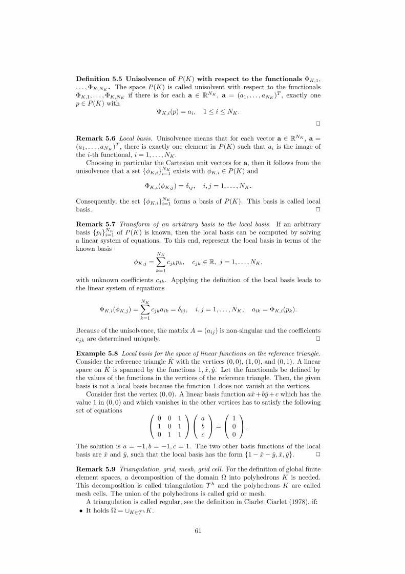
Example 5.8 Local basis for the space of linear functions on the reference triangle.Consider the reference triangle K with the vertices (0, 0), (1, 0), and (0, 1). A linearspace on K is spanned by the functions 1, x, y. Let the functionals be defined bythe values of the functions in the vertices of the reference triangle. Then, the givenbasis is not a local basis because the function 1 does not vanish at the vertices.

Consider first the vertex (0, 0). A linear basis function ax+ by+ c which has thevalue 1 in (0, 0) and which vanishes in the other vertices has to satisfy the followingset of equations

0 0 11 0 10 1 1

abc

=

100

.

The solution is a = −1, b = −1, c = 1. The two other basis functions of the localbasis are x and y, such that the local basis has the form 1− x− y, x, y.

Remark 5.9 Triangulation, grid, mesh, grid cell. For the definition of global finiteelement spaces, a decomposition of the domain Ω into polyhedrons K is needed.This decomposition is called triangulation T h and the polyhedrons K are calledmesh cells. The union of the polyhedrons is called grid or mesh.

A triangulation is called regular, see the definition in Ciarlet Ciarlet (1978), if:

• It holds Ω = ∪K∈T hK.

61

• Each mesh cell K ∈ T h is closed and the interior K is non-empty.• For distinct mesh cells K1 and K2 there holds K1 ∩ K2 = ∅.• For each K ∈ T h, the boundary ∂K is Lipschitz-continuous.• The intersection of two mesh cells is either empty or a common m-face, m ∈0, . . . , d− 1.

Remark 5.10 Global and local functionals. Let Φ1, . . . ,ΦN : Cs(Ω) → R contin-uous linear functionals of the same types as given in Remark 5.4. The restrictionof the functionals to Cs(K) defines local functionals ΦK,1, . . . ,ΦK,NK

, where it isassumed that the local functionals are unisolvent on P (K). The union of all meshcells Kj , for which there is a p ∈ P (Kj) with Φi(p) 6= 0, will be denoted by ωi.

Example 5.11 On subdomains ωi. Consider the two-dimensional case and let Φi

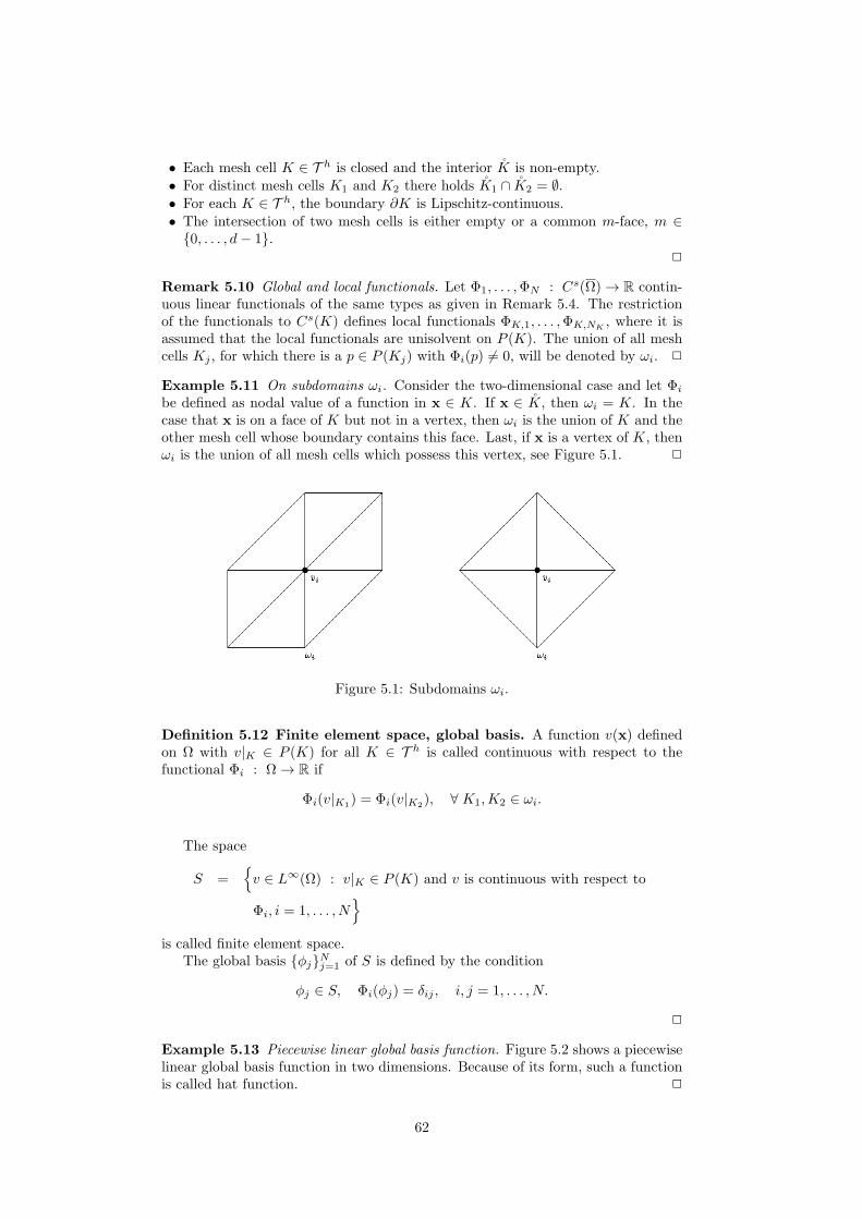
be defined as nodal value of a function in x ∈ K. If x ∈ K, then ωi = K. In thecase that x is on a face of K but not in a vertex, then ωi is the union of K and theother mesh cell whose boundary contains this face. Last, if x is a vertex of K, thenωi is the union of all mesh cells which possess this vertex, see Figure 5.1.

Figure 5.1: Subdomains ωi.

Definition 5.12 Finite element space, global basis. A function v(x) definedon Ω with v|K ∈ P (K) for all K ∈ T h is called continuous with respect to thefunctional Φi : Ω → R if

Φi(v|K1) = Φi(v|K2

), ∀ K1,K2 ∈ ωi.

The space

S =

v ∈ L∞(Ω) : v|K ∈ P (K) and v is continuous with respect to

Φi, i = 1, . . . , N

is called finite element space.The global basis φj

Nj=1 of S is defined by the condition

φj ∈ S, Φi(φj) = δij , i, j = 1, . . . , N.

Example 5.13 Piecewise linear global basis function. Figure 5.2 shows a piecewiselinear global basis function in two dimensions. Because of its form, such a functionis called hat function.

62

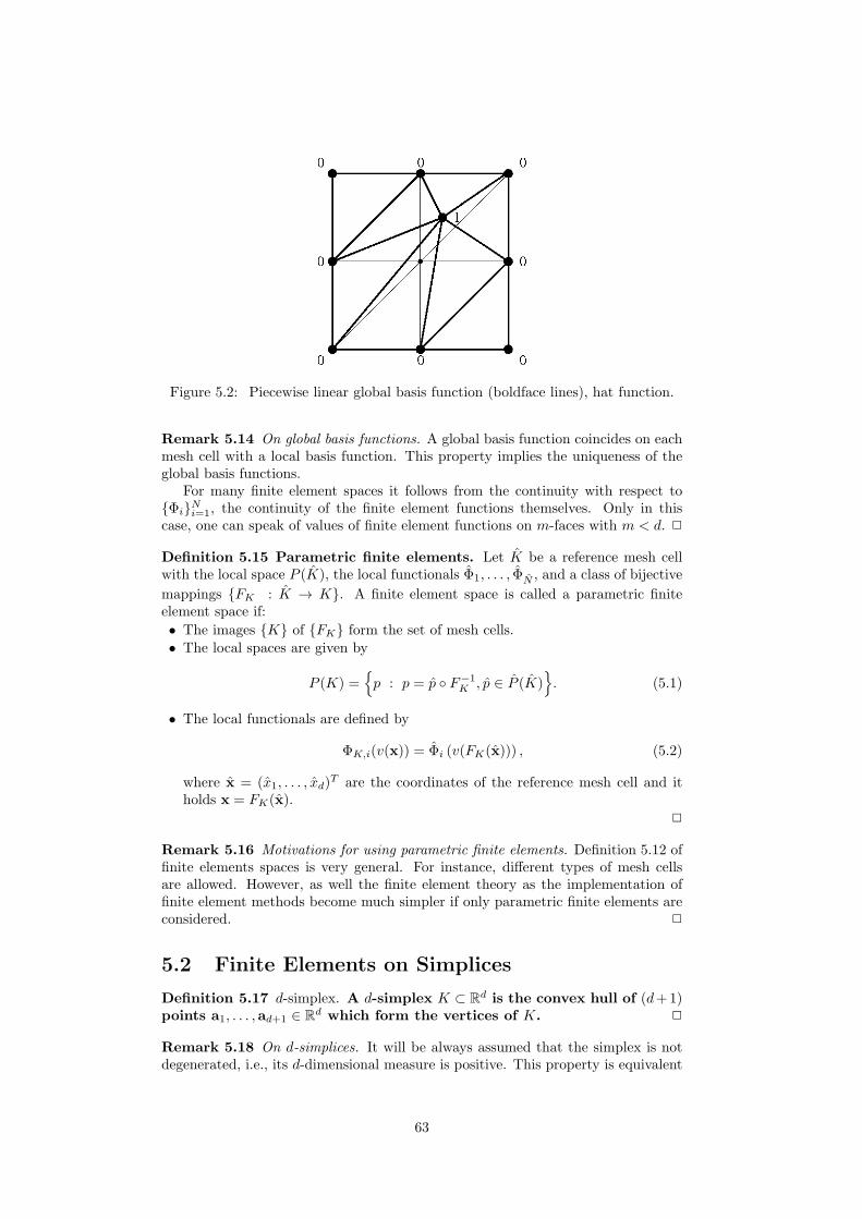
Figure 5.2: Piecewise linear global basis function (boldface lines), hat function.

Remark 5.14 On global basis functions. A global basis function coincides on eachmesh cell with a local basis function. This property implies the uniqueness of theglobal basis functions.

For many finite element spaces it follows from the continuity with respect toΦi

Ni=1, the continuity of the finite element functions themselves. Only in this

case, one can speak of values of finite element functions on m-faces with m < d.

Definition 5.15 Parametric finite elements. Let K be a reference mesh cellwith the local space P (K), the local functionals Φ1, . . . , ΦN , and a class of bijective

mappings FK : K → K. A finite element space is called a parametric finiteelement space if:

• The images K of FK form the set of mesh cells.• The local spaces are given by

P (K) =

p : p = p F−1K , p ∈ P (K)

. (5.1)

• The local functionals are defined by

ΦK,i(v(x)) = Φi (v(FK(x))) , (5.2)

where x = (x1, . . . , xd)T are the coordinates of the reference mesh cell and it

holds x = FK(x).

Remark 5.16 Motivations for using parametric finite elements. Definition 5.12 offinite elements spaces is very general. For instance, different types of mesh cellsare allowed. However, as well the finite element theory as the implementation offinite element methods become much simpler if only parametric finite elements areconsidered.

5.2 Finite Elements on Simplices

Definition 5.17 d-simplex. A d-simplex K ⊂ Rd is the convex hull of (d+1)

points a1, . . . ,ad+1 ∈ Rd which form the vertices of K.

Remark 5.18 On d-simplices. It will be always assumed that the simplex is notdegenerated, i.e., its d-dimensional measure is positive. This property is equivalent

63

to the non-singularity of the matrix

A =

a11 a12 . . . a1,d+1

a21 a22 . . . a2,d+1

......

. . ....

ad1 ad2 . . . ad,d+1

1 1 . . . 1

,

where ai = (a1i, a2i, . . . , adi)T , i = 1, . . . , d+ 1.

For d = 2, the simplices are the triangles and for d = 3 they are the tetrahedrons.

Definition 5.19 Barycentric coordinates. Since K is the convex hull of thepoints ai

d+1i=1 , the parametrization of K with a convex combination of the vertices

reads as follows

K =

x ∈ Rd : x =

d+1∑

i=1

λiai, 0 ≤ λi ≤ 1,

d+1∑

i=1

λi = 1

.

The coefficients λ1, . . . , λd+1 are called barycentric coordinates of x ∈ K.

Remark 5.20 On barycentric coordinates. From the definition it follows that thebarycentric coordinates are the solution of the linear system of equations

d+1∑

i=1

ajiλi = xj , 1 ≤ j ≤ d,

d+1∑

i=1

λi = 1.

Since the system matrix is non-singular, see Remark 5.18, the barycentric coordi-nates are determined uniquely.

The barycentric coordinates of the vertex ai, i = 1, . . . , d+ 1, of the simplex isλi = 1 and λj = 0 if i 6= j. Since λi(aj) = δij , the barycentric coordinate λi can beidentified with the linear function which has the value 1 in the vertex ai and whichvanishes in all other vertices aj with j 6= i.

The barycenter of the simplex is given by

SK =1

d+ 1

d+1∑

i=1

ai =

d+1∑

i=1

1

d+ 1ai.

Hence, its barycentric coordinates are λi = 1/(d+ 1), i = 1, . . . , d+ 1.

Remark 5.21 Simplicial reference mesh cells. A commonly used reference meshcell for triangles and tetrahedrons is the unit simplex

K =

x ∈ Rd :

d∑

i=1

xi ≤ 1, xi ≥ 0, i = 1, . . . , d

,

see Figure 5.3. The class FK of admissible mappings are the bijective affinemappings

FK x = Bx+ b, B ∈ Rd×d, det(B) 6= 0, b ∈ R

d.

The images of these mappings generate the set of the non-degenerated simplicesK ⊂ R

d.

64

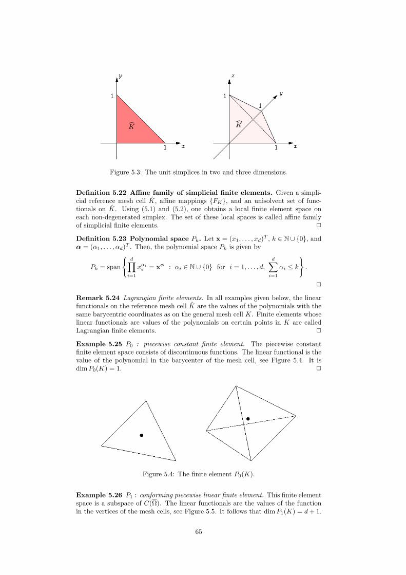
Figure 5.3: The unit simplices in two and three dimensions.

Definition 5.22 Affine family of simplicial finite elements. Given a simpli-cial reference mesh cell K, affine mappings FK, and an unisolvent set of func-tionals on K. Using (5.1) and (5.2), one obtains a local finite element space oneach non-degenerated simplex. The set of these local spaces is called affine familyof simplicial finite elements.

Definition 5.23 Polynomial space Pk. Let x = (x1, . . . , xd)T , k ∈ N∪ 0, and

α = (α1, . . . , αd)T . Then, the polynomial space Pk is given by

Pk = span

d∏

i=1

xαii = xα : αi ∈ N ∪ 0 for i = 1, . . . , d,

d∑

i=1

αi ≤ k

.

Remark 5.24 Lagrangian finite elements. In all examples given below, the linearfunctionals on the reference mesh cell K are the values of the polynomials with thesame barycentric coordinates as on the general mesh cell K. Finite elements whoselinear functionals are values of the polynomials on certain points in K are calledLagrangian finite elements.

Example 5.25 P0 : piecewise constant finite element. The piecewise constantfinite element space consists of discontinuous functions. The linear functional is thevalue of the polynomial in the barycenter of the mesh cell, see Figure 5.4. It isdimP0(K) = 1.

Figure 5.4: The finite element P0(K).

Example 5.26 P1 : conforming piecewise linear finite element. This finite elementspace is a subspace of C(Ω). The linear functionals are the values of the functionin the vertices of the mesh cells, see Figure 5.5. It follows that dimP1(K) = d+ 1.

65

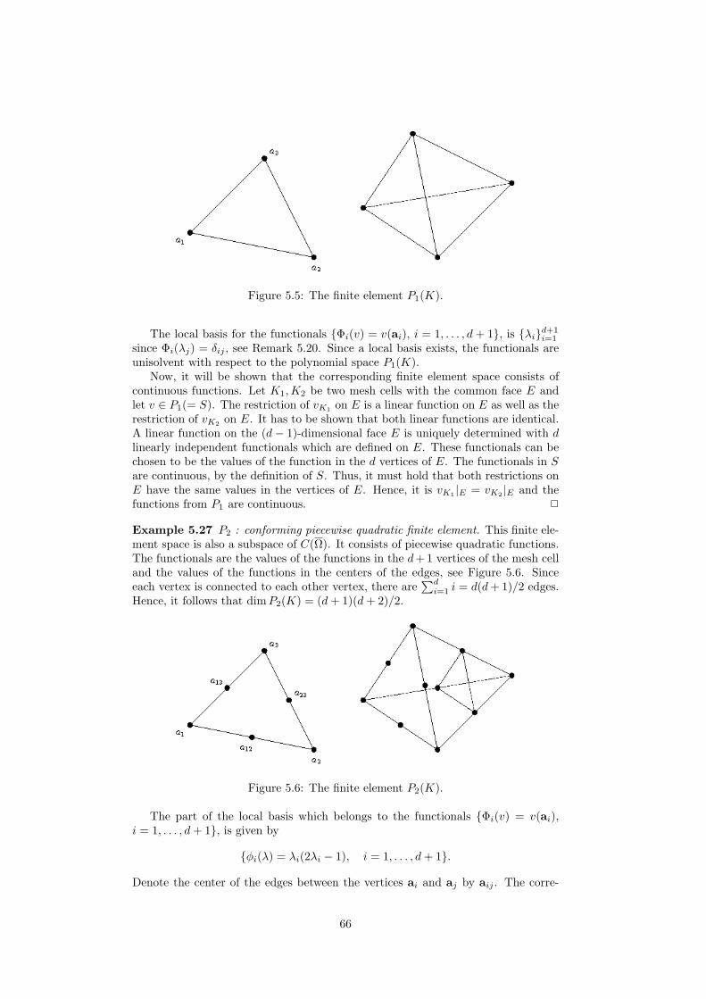
Figure 5.5: The finite element P1(K).

The local basis for the functionals Φi(v) = v(ai), i = 1, . . . , d + 1, is λid+1i=1

since Φi(λj) = δij , see Remark 5.20. Since a local basis exists, the functionals areunisolvent with respect to the polynomial space P1(K).

Now, it will be shown that the corresponding finite element space consists ofcontinuous functions. Let K1,K2 be two mesh cells with the common face E andlet v ∈ P1(= S). The restriction of vK1 on E is a linear function on E as well as therestriction of vK2 on E. It has to be shown that both linear functions are identical.A linear function on the (d− 1)-dimensional face E is uniquely determined with dlinearly independent functionals which are defined on E. These functionals can bechosen to be the values of the function in the d vertices of E. The functionals in Sare continuous, by the definition of S. Thus, it must hold that both restrictions onE have the same values in the vertices of E. Hence, it is vK1 |E = vK2 |E and thefunctions from P1 are continuous.

Example 5.27 P2 : conforming piecewise quadratic finite element. This finite ele-ment space is also a subspace of C(Ω). It consists of piecewise quadratic functions.The functionals are the values of the functions in the d+1 vertices of the mesh celland the values of the functions in the centers of the edges, see Figure 5.6. Sinceeach vertex is connected to each other vertex, there are

∑di=1 i = d(d+ 1)/2 edges.

Hence, it follows that dimP2(K) = (d+ 1)(d+ 2)/2.

Figure 5.6: The finite element P2(K).

The part of the local basis which belongs to the functionals Φi(v) = v(ai),i = 1, . . . , d+ 1, is given by

φi(λ) = λi(2λi − 1), i = 1, . . . , d+ 1.

Denote the center of the edges between the vertices ai and aj by aij . The corre-

66

sponding part of the local basis is given by

φij = 4λiλj , i, j = 1, . . . , d+ 1, i < j.

The unisolvence follows from the fact that there exists a local basis. The continuityof the corresponding finite element space is shown in the same way as for the P1

finite element. The restriction of a quadratic function in a mesh cell to a face E isa quadratic function on that face. Hence, the function on E is determined uniquelywith d(d+ 1)/2 linearly independent functionals on E.

The functions φij are called in two dimensions edge bubble functions.

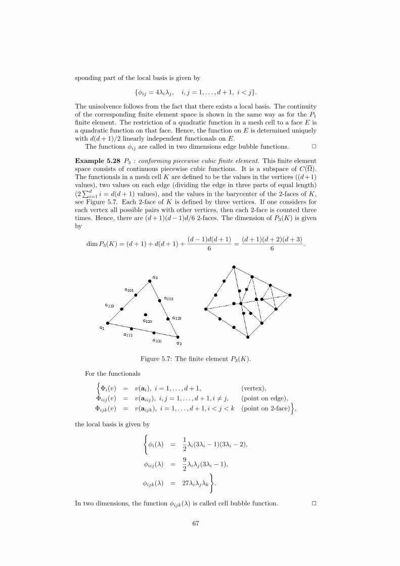
Example 5.28 P3 : conforming piecewise cubic finite element. This finite elementspace consists of continuous piecewise cubic functions. It is a subspace of C(Ω).The functionals in a mesh cell K are defined to be the values in the vertices ((d+1)values), two values on each edge (dividing the edge in three parts of equal length)

(2∑d

i=1 i = d(d + 1) values), and the values in the barycenter of the 2-faces of K,see Figure 5.7. Each 2-face of K is defined by three vertices. If one considers foreach vertex all possible pairs with other vertices, then each 2-face is counted threetimes. Hence, there are (d+ 1)(d− 1)d/6 2-faces. The dimension of P3(K) is givenby

dimP3(K) = (d+ 1) + d(d+ 1) +(d− 1)d(d+ 1)

6=

(d+ 1)(d+ 2)(d+ 3)

6.

Figure 5.7: The finite element P3(K).

For the functionals

Φi(v) = v(ai), i = 1, . . . , d+ 1, (vertex),

Φiij(v) = v(aiij), i, j = 1, . . . , d+ 1, i 6= j, (point on edge),

Φijk(v) = v(aijk), i = 1, . . . , d+ 1, i < j < k (point on 2-face)

,

the local basis is given by

φi(λ) =1

2λi(3λi − 1)(3λi − 2),

φiij(λ) =9

2λiλj(3λi − 1),

φijk(λ) = 27λiλjλk

.

In two dimensions, the function φijk(λ) is called cell bubble function.

67

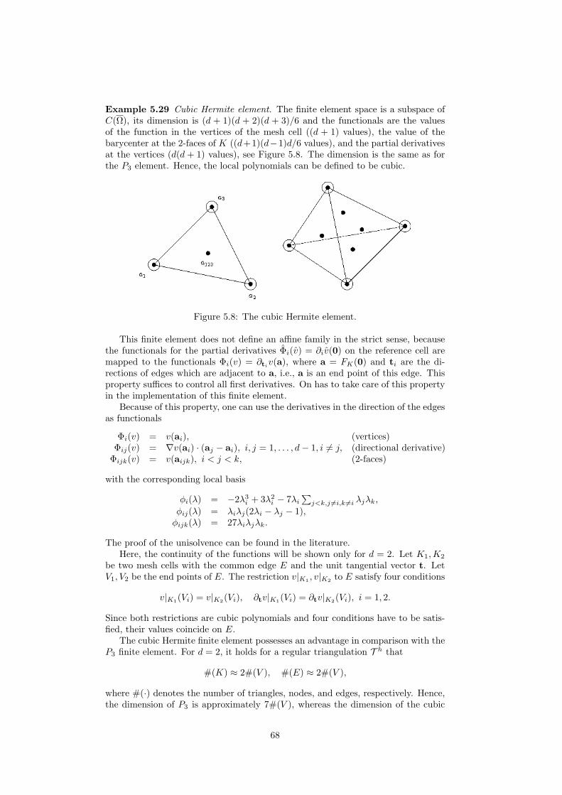
Example 5.29 Cubic Hermite element. The finite element space is a subspace ofC(Ω), its dimension is (d + 1)(d + 2)(d + 3)/6 and the functionals are the valuesof the function in the vertices of the mesh cell ((d + 1) values), the value of thebarycenter at the 2-faces of K ((d+1)(d−1)d/6 values), and the partial derivativesat the vertices (d(d + 1) values), see Figure 5.8. The dimension is the same as forthe P3 element. Hence, the local polynomials can be defined to be cubic.

Figure 5.8: The cubic Hermite element.

This finite element does not define an affine family in the strict sense, becausethe functionals for the partial derivatives Φi(v) = ∂iv(0) on the reference cell aremapped to the functionals Φi(v) = ∂tiv(a), where a = FK(0) and ti are the di-rections of edges which are adjacent to a, i.e., a is an end point of this edge. Thisproperty suffices to control all first derivatives. On has to take care of this propertyin the implementation of this finite element.

Because of this property, one can use the derivatives in the direction of the edgesas functionals

Φi(v) = v(ai), (vertices)Φij(v) = ∇v(ai) · (aj − ai), i, j = 1, . . . , d− 1, i 6= j, (directional derivative)Φijk(v) = v(aijk), i < j < k, (2-faces)

with the corresponding local basis

φi(λ) = −2λ3i + 3λ2i − 7λi∑

j<k,j 6=i,k 6=i λjλk,

φij(λ) = λiλj(2λi − λj − 1),φijk(λ) = 27λiλjλk.

The proof of the unisolvence can be found in the literature.Here, the continuity of the functions will be shown only for d = 2. Let K1,K2

be two mesh cells with the common edge E and the unit tangential vector t. LetV1, V2 be the end points of E. The restriction v|K1

, v|K2to E satisfy four conditions

v|K1(Vi) = v|K2

(Vi), ∂tv|K1(Vi) = ∂tv|K2

(Vi), i = 1, 2.

Since both restrictions are cubic polynomials and four conditions have to be satis-fied, their values coincide on E.

The cubic Hermite finite element possesses an advantage in comparison with theP3 finite element. For d = 2, it holds for a regular triangulation T h that

#(K) ≈ 2#(V ), #(E) ≈ 2#(V ),

where #(·) denotes the number of triangles, nodes, and edges, respectively. Hence,the dimension of P3 is approximately 7#(V ), whereas the dimension of the cubic

68

Hermite element is approximately 5#(V ). This difference comes from the fact thatboth spaces are different. The elements of both spaces are continuous functions,but for the functions of the cubic Hermite finite element, in addition, the firstderivatives are continuous at the nodes. That means, these two spaces are differentfinite element spaces whose degree of the local polynomial space is the same (cubic).One can see at this example the importance of the functionals for the definition ofthe global finite element space.

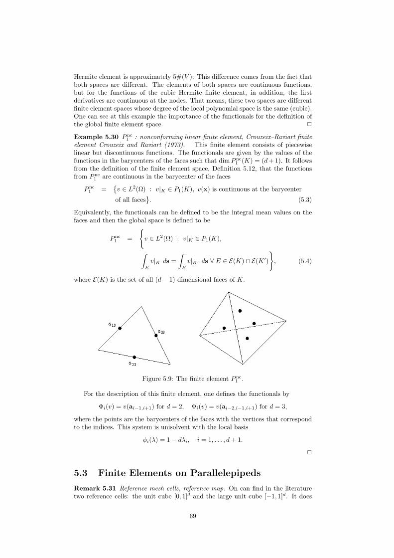
Example 5.30 P nc1 : nonconforming linear finite element, Crouzeix–Raviart finite

element Crouzeix and Raviart (1973). This finite element consists of piecewiselinear but discontinuous functions. The functionals are given by the values of thefunctions in the barycenters of the faces such that dimP nc

1 (K) = (d+1). It followsfrom the definition of the finite element space, Definition 5.12, that the functionsfrom P nc

1 are continuous in the barycenter of the faces

P nc1 =

v ∈ L2(Ω) : v|K ∈ P1(K), v(x) is continuous at the barycenter

of all faces. (5.3)

Equivalently, the functionals can be defined to be the integral mean values on thefaces and then the global space is defined to be

P nc1 =

v ∈ L2(Ω) : v|K ∈ P1(K),

∫

E

v|K ds =

∫

E

v|K′ ds ∀ E ∈ E(K) ∩ E(K ′)

, (5.4)

where E(K) is the set of all (d− 1) dimensional faces of K.

Figure 5.9: The finite element P nc1 .

For the description of this finite element, one defines the functionals by

Φi(v) = v(ai−1,i+1) for d = 2, Φi(v) = v(ai−2,i−1,i+1) for d = 3,

where the points are the barycenters of the faces with the vertices that correspondto the indices. This system is unisolvent with the local basis

φi(λ) = 1− dλi, i = 1, . . . , d+ 1.

5.3 Finite Elements on Parallelepipeds

Remark 5.31 Reference mesh cells, reference map. On can find in the literaturetwo reference cells: the unit cube [0, 1]d and the large unit cube [−1, 1]d. It does

69

not matter which reference cell is chosen. Here, the large unit cube will be used:K = [−1, 1]d. The class of admissible reference maps FK consists of bijectiveaffine mappings of the form

FK x = Bx+ b, B ∈ Rd×d, b ∈ R

d.

If B is a diagonal matrix, then K is mapped to d-rectangles.The class of mesh cells which are obtained in this way is not sufficient to tri-

angulate general domains. If one wants to use more general mesh cells than par-allelepipeds, then the class of admissible reference maps has to be enlarged, seeSection 5.4.

Definition 5.32 Polynomial space Qk. Let x = (x1, . . . , xd)T and denote by

α = (α1, . . . , αd)T a multi-index. Then, the polynomial space Qk is given by

Qk = span

d∏

i=1

xαii = xα : 0 ≤ αi ≤ k for i = 1, . . . , d

.

Example 5.33 Q1 vs. P1. The space Q1 consists of all polynomials which ared-linear. Let d = 2, then it is

Q1 = span1, x, y, xy,

whereasP1 = span1, x, y.

Remark 5.34 Finite elements on d-rectangles. For simplicity of presentation, theexamples below consider d-rectangles. In this case, the finite elements are just tensorproducts of one-dimensional finite elements. In particular, the basis functions canbe written as products of one-dimensional basis functions.

Example 5.35 Q0 : piecewise constant finite element. Similarly to the P0 space,the space Q0 consists of piecewise constant, discontinuous functions. The functionalis the value of the function in the barycenter of the mesh cell K and it holdsdimQ0(K) = 1.

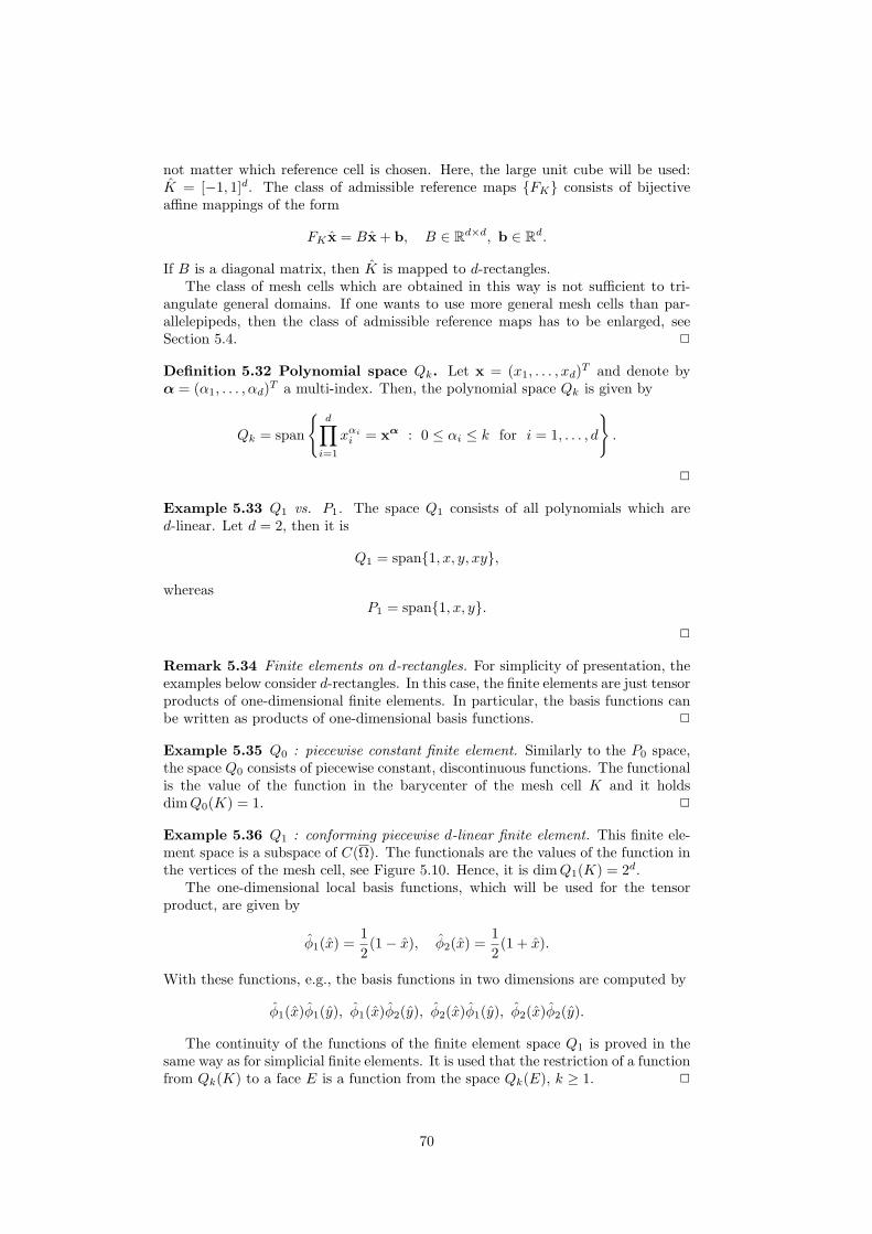
Example 5.36 Q1 : conforming piecewise d-linear finite element. This finite ele-ment space is a subspace of C(Ω). The functionals are the values of the function inthe vertices of the mesh cell, see Figure 5.10. Hence, it is dimQ1(K) = 2d.

The one-dimensional local basis functions, which will be used for the tensorproduct, are given by

φ1(x) =1

2(1− x), φ2(x) =

1

2(1 + x).

With these functions, e.g., the basis functions in two dimensions are computed by

φ1(x)φ1(y), φ1(x)φ2(y), φ2(x)φ1(y), φ2(x)φ2(y).

The continuity of the functions of the finite element space Q1 is proved in thesame way as for simplicial finite elements. It is used that the restriction of a functionfrom Qk(K) to a face E is a function from the space Qk(E), k ≥ 1.

70

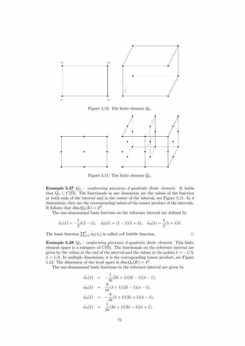
Figure 5.10: The finite element Q1.

Figure 5.11: The finite element Q2.

Example 5.37 Q2 : conforming piecewise d-quadratic finite element. It holdsthat Q2 ⊂ C(Ω). The functionals in one dimension are the values of the functionat both ends of the interval and in the center of the interval, see Figure 5.11. In ddimensions, they are the corresponding values of the tensor product of the intervals.It follows that dimQ2(K) = 3d.

The one-dimensional basis function on the reference interval are defined by

φ1(x) = −1

2x(1− x), φ2(x) = (1− x)(1 + x), φ3(x) =

1

2(1 + x)x.

The basis function∏d

i=1 φ2(xi) is called cell bubble function.

Example 5.38 Q3 : conforming piecewise d-quadratic finite element. This finiteelement space is a subspace of C(Ω). The functionals on the reference interval aregiven by the values at the end of the interval and the values at the points x = −1/3,x = 1/3. In multiple dimensions, it is the corresponding tensor product, see Figure5.12. The dimension of the local space is dimQ3(K) = 4d.

The one-dimensional basis functions in the reference interval are given by

φ1(x) = −1

16(3x+ 1)(3x− 1)(x− 1),

φ2(x) =9

16(x+ 1)(3x− 1)(x− 1),

φ3(x) = −9

16(x+ 1)(3x+ 1)(x− 1),

φ4(x) =1

16(3x+ 1)(3x− 1)(x+ 1).

71

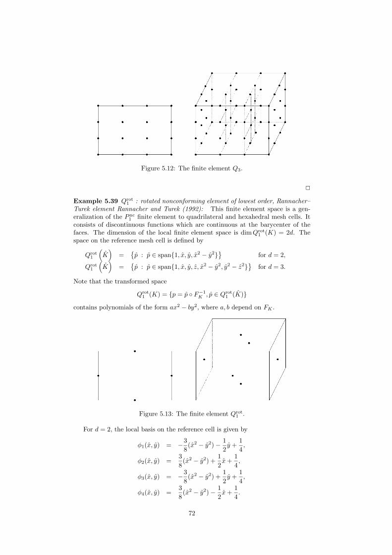
Figure 5.12: The finite element Q3.

Example 5.39 Qrot1 : rotated nonconforming element of lowest order, Rannacher–

Turek element Rannacher and Turek (1992): This finite element space is a gen-eralization of the P nc

1 finite element to quadrilateral and hexahedral mesh cells. Itconsists of discontinuous functions which are continuous at the barycenter of thefaces. The dimension of the local finite element space is dimQrot

1 (K) = 2d. Thespace on the reference mesh cell is defined by

Qrot1

(

K)

=p : p ∈ span1, x, y, x2 − y2

for d = 2,

Qrot1

(

K)

=p : p ∈ span1, x, y, z, x2 − y2, y2 − z2

for d = 3.

Note that the transformed space

Qrot1 (K) = p = p F−1

K , p ∈ Qrot1 (K)

contains polynomials of the form ax2 − by2, where a, b depend on FK .

Figure 5.13: The finite element Qrot1 .

For d = 2, the local basis on the reference cell is given by

φ1(x, y) = −3

8(x2 − y2)−

1

2y +

1

4,

φ2(x, y) =3

8(x2 − y2) +

1

2x+

1

4,

φ3(x, y) = −3

8(x2 − y2) +

1

2y +

1

4,

φ4(x, y) =3

8(x2 − y2)−

1

2x+

1

4.

72

Analogously to the Crouzeix–Raviart finite element, the functionals can be de-fined as point values of the functions in the barycenters of the faces, see Figure 5.13,or as integral mean values of the functions at the faces. Consequently, the finiteelement spaces are defined in the same way as (5.3) or (5.4), with P nc

1 (K) replacedby Qrot

1 (K).In the code MooNMD John and Matthies (2004), the mean value oriented

Qrot1 finite element space is implemented fro two dimensions and the point value

oriented Qrot1 finite element space for three dimensions. For d = 3, the integrals on

the faces of mesh cells, whose equality is required in the mean value oriented Qrot1

finite element space, involve a weighting function which depends on the particularmesh cell K. The computation of these weighting functions for all mesh cells is anadditional computational overhead. For this reason, Schieweck (Schieweck, 1997,p. 21) suggested to use for d = 3 the simpler point value oriented form of the Qrot

1

finite element.

5.4 Parametric Finite Elements on General d-Di-

mensional Quadrilaterals

Remark 5.40 Parametric mappings. The image of an affine mapping of the refer-ence mesh cell K = [−1, 1]d, d ∈ 2, 3, is a parallelepiped. If one wants to considerfinite elements on general q-quadrilaterals, then the class of admissible referencemaps has to be enlarged.

The simplest parametric finite element on quadrilaterals in two dimensions usesbilinear mappings. Let K = [−1, 1]2 and let

FK(x) =

(F 1K(x)F 2K(x)

)

=

(a11 + a12x+ a13y + a14xya21 + a22x+ a23y + a24xy

)

, F iK ∈ Q1, i = 1, 2,

be a bilinear mapping from K on the class of admissible quadrilaterals. A quadri-lateral K is called admissible if

• the length of all edges of K is larger than zero,• the interior angles of K are smaller than π, i.e. K is convex.

This class contains, e.g., trapezoids and rhombi.

Remark 5.41 Parametric finite element functions. The functions of the localspace P (K) on the mesh cell K are defined by p = p F−1

K . These functionsare in general rational functions. However, using d-linear mappings, then the re-striction of FK on an edge of K is an affine map. For instance, in the case of theQ1 finite element, the functions on K are linear functions on each edge of K forthis reason. It follows that the functions of the corresponding finite element spaceare continuous, see Example 5.26.

5.5 Transform of Integrals

Remark 5.42 Motivation. The transform of integrals from the reference meshcell to mesh cells of the grid and vice versa is used as well for analysis as for theimplementation of finite element methods. This section provides an overview of themost important formulae for transforms.

Let K ⊂ Rd be the reference mesh cell, K be an arbitrary mesh cell, and

FK : K → K with x = FK(x) be the reference map. It is assumed that thereference map is a continuous differentiable one-to-one map. The inverse map is

73

denoted by F−1K : K → K. For the integral transforms, the derivatives (Jacobians)

of FK and F−1K are needed

DFK(x)ij =∂xi∂xj

, DF−1K (x)ij =

∂xi∂xj

, i, j = 1, . . . , d.

Remark 5.43 Integral with a function without derivatives. This integral trans-forms with the standard rule of integral transforms

∫

K

v(x) dx =

∫

K

v(x) |detDFK(x)| dx, (5.5)

where v(x) = v(FK(x)).

Remark 5.44 Transform of derivatives. Using the chain rule, one obtains

∂v

∂xi(x) =

d∑

j=1

∂v

∂xj(x)

∂xj∂xi

= ∇xv(x) ·((DF−1

K (x))T)

i

= ∇xv(x) ·((DF−1

K (FK(x)))T)

i, (5.6)

∂v

∂x(x) =

d∑

j=1

∂v

∂xj(x)

∂xj∂xi

= ∇v(x) ·(

(DFK(x))T)

i

= ∇v(x) ·((DFK(F−1

K (x)))T)

i. (5.7)

The index i denotes the i-th row of a matrix. Derivatives on the reference mesh cellare marked with a symbol on the operator.

Remark 5.45 Integrals with a gradients. Using the rule for transforming integralsand (5.6) gives

∫

K

b(x) · ∇v(x) dx

=

∫

K

b (FK(x)) ·[(DF−1

K

)T(FK(x))

]

∇xv(x) |detDFK(x)| dx. (5.8)

Similarly, one obtains∫

K

∇v(x) · ∇w(x) dx

=

∫

K

[(DF−1

K

)T(FK(x))

]

∇xv(x) ·[(DF−1

K

)T(FK(x))

]

∇xw(x)

× |detDFK(x)| dx. (5.9)

Remark 5.46 Integral with the divergence. Integrals of the following type areimportant for the Navier–Stokes equations

∫

K

∇ · v(x)q(x) dx =

∫

K

d∑

i=1

∂vi∂xi

(x)q(x) dx

=

∫

K

d∑

i=1

[((DF−1

K (FK(x)))T)

i· ∇xvi(x)

]

q(x) |detDFK(x)| dx

=

∫

K

[(DF−1

K (FK(x)))T

: Dxv(x)]

q(x) |detDFK(x)| dx. (5.10)

In the derivation, (5.6) was used.

74

Example 5.47 Affine transform. The most important class of reference maps areaffine transforms

x = Bx+ b, B ∈ Rd×d,b ∈ R

d,

where the invertible matrix B and the vector b are constants. It follows that

x = B−1 (x− b) = B−1x−B−1b.

In this case, there are

DFK = B, DF−1K = B−1, detDFK = det(B).

One obtains for the integral transforms from (5.5), (5.8), (5.9), and (5.10)

∫

K

v(x) dx = |det(B)|

∫

K

v(x) dx, (5.11)

∫

K

b(x) · ∇v(x) dx = |det(B)|

∫

K

b (FK(x)) ·B−T∇xv(x) dx, (5.12)

∫

K

∇v(x) · ∇w(x) dx = |det(B)|

∫

K

B−T∇xv(x) ·B−T∇xw(x) dx, (5.13)

∫

K

∇ · v(x)q(x) dx = |det(B)|

∫

K

[B−T : Dxv(x)

]q(x) dx. (5.14)

75

Chapter 6

Interpolation

Remark 6.1 Motivation. Variational forms of partial differential equations usefunctions in Sobolev spaces. The solution of these equations shall be approximatedwith the Ritz method in finite dimensional spaces, the finite element spaces. Thebest possible approximation of an arbitrary function from the Sobolev space by afinite element function is a factor in the upper bound for the finite element error,e.g., see the Lemma of Cea, estimate (4.19).

This section studies the approximation quality of finite element spaces. Esti-mates are proved for interpolants of functions. Interpolation estimates are of courseupper bounds for the best approximation error and they can serve as factors infinite element error estimates.

6.1 Interpolation in Sobolev Spaces by Polynomi-

als

Lemma 6.2 Unique determination of a polynomial with integral condi-

tions. Let Ω be a bounded domain in Rd with Lipschitz boundary. Let m ∈ N∪0

be given and let for all derivatives with multi-index α, |α| ≤ m, a value aα ∈ R begiven. Then, there is a uniquely determined polynomial p ∈ Pm(Ω) such that

∫

Ω

∂αp(x) dx = aα, |α| ≤ m. (6.1)

Proof: Let p ∈ Pm(Ω) be an arbitrary polynomial. It has the form

p(x) =∑

|β|≤m

bβxβ.

Inserting this representation into (6.1) leads to a linear system of equations Mb = a with

M = (Mαβ), Mαβ =

∫

Ω

∂αxβ dx, b = (bβ), a = (aα),

for |α| , |β| ≤ m. Since M is a squared matrix, the linear system of equations possesses aunique solution if and only if M is non-singular.

The proof is performed by contradiction. Assume that M is singular. Then thereexists a non-trivial solution of the homogeneous system. That means, there is a polynomialq ∈ Pm(Ω) \ 0 with

∫

Ω

∂αq(x) dx = 0 for all |α| ≤ m.

The polynomial q(x) has the representation q(x) =∑

|β|≤m cβxβ. Now, one can choose a

cβ 6= 0 with maximal value |β|. Then, it is ∂βq(x) = Ccβ = const 6= 0, where C > 0 comes

76

from the differentiation rule for polynomials, which is a contradiction to the vanishing of

the integral for ∂βq(x).

Remark 6.3 To Lemma 6.2. Lemma 6.2 states that a polynomial is uniquelydetermined if a condition on the integral on Ω is prescribed for each derivative.

Lemma 6.4 Poincare-type inequality. Denote by Dkv(x), k ∈ N ∪ 0, thetotal derivative of order k of a function v(x), e.g., for k = 1 the gradient of v(x).Let Ω be convex and be included into a ball of radius R. Let k, l ∈ N ∪ 0 withk ≤ l and let p ∈ R with p ∈ [1,∞]. Assume that v ∈W l,p(Ω) satisfies

∫

Ω

∂αv(x) dx = 0 for all |α| ≤ l − 1,

then it holds the estimate∥∥Dkv

∥∥Lp(Ω)

≤ CRl−k∥∥Dlv

∥∥Lp(Ω)

,

where the constant C does not depend on Ω and on v(x).

Proof: There is nothing to prove if k = l. In addition, it suffices to prove the lemmafor k = 0 and l = 1, since the general case follows by applying the result to ∂αv(x). Onlythe case p < ∞ will be discussed here in detail.

Since Ω is assumed to be convex, the integral mean value theorem can be written inthe form

v(x)− v(y) =

∫ 1

0

∇v(tx+ (1− t)y) · (x− y) dt, x,y ∈ Ω.

Integration with respect to y yields

v(x)

∫

Ω

dy −

∫

Ω

v(y) dy =

∫

Ω

∫ 1

0

∇v(tx+ (1− t)y) · (x− y) dt dy.

It follows from the assumption that the second integral on the left hand side vanishes.Hence, one gets

v(x) =1

|Ω|

∫

Ω

∫ 1

0

∇v(tx+ (1− t)y) · (x− y) dt dy.

Now, taking the absolute value on both sides, using that the absolute value of an integral isestimated from above by the integral of the absolute value, applying the Cauchy–Schwarzinequality for vectors and the estimate ‖x− y‖2 ≤ 2R yields

|v(x)| =1

|Ω|

∣∣∣∣

∫

Ω

∫ 1

0

∇v(tx+ (1− t)y) · (x− y) dt dy

∣∣∣∣

≤1

|Ω|

∫

Ω

∫ 1

0

|∇v(tx+ (1− t)y) · (x− y)| dt dy

≤2R

|Ω|

∫

Ω

∫ 1

0

‖∇v(tx+ (1− t)y)‖2 dt dy. (6.2)

Then (6.2) is raised to the power p and then integrated with respect to x. One obtainswith Holder’s inequality (3.4), with p−1 + q−1 = 1 =⇒ p/q − p = p(1/q − 1) = −1, that

∫

Ω

|v(x)|p dx ≤CRp

|Ω|p

∫

Ω

(∫

Ω

∫ 1

0

‖∇v(tx+ (1− t)y)‖2 dt dy

)p

dx

≤CRp

|Ω|p

∫

Ω

[(∫

Ω

∫ 1

0

1q dt dy

)p/q

︸ ︷︷ ︸

|Ω|p/q

×

(∫

Ω

∫ 1

0

‖∇v(tx+ (1− t)y)‖p2 dt dy

)]

dx

=CRp

|Ω|

∫

Ω

(∫

Ω

∫ 1

0

‖∇v(tx+ (1− t)y)‖p2 dt dy

)

dx.

77

Applying the theorem of Fubini allows the commutation of the integration

∫

Ω

|v(x)|p dx ≤CRp

|Ω|

∫ 1

0

∫

Ω

(∫

Ω

‖∇v(tx+ (1− t)y)‖p2 dy

)

dx dt.

Using the integral mean value theorem in one dimension gives that there is a t0 ∈ [0, 1],such that

∫

Ω

|v(x)|p dx ≤CRp

|Ω|

∫

Ω

(∫

Ω

‖∇v(t0x+ (1− t0)y)‖p2 dy

)

dx.

The function ‖∇v(x)‖p2 will be extended to Rd by zero and the extension will be also

denoted by ‖∇v(x)‖p2. Then, it is

∫

Ω

|v(x)|p dx ≤CRp

|Ω|

∫

Ω

(∫

Rd

‖∇v(t0x+ (1− t0)y)‖p2 dy

)

dx. (6.3)

Let t0 ∈ [0, 1/2]. Since the domain of integration is Rd, a substitution of variables

t0x+ (1− t0)y = z can be applied and leads to∫

Rd

‖∇v(t0x+ (1− t0)y)‖p2 dy =

1

1− t0

∫

Rd

‖∇v(z)‖p2 dz ≤ 2 ‖∇v‖pLp(Ω) ,

since 1/(1− t0) ≤ 2. Inserting this expression into (6.3) gives∫

Ω

|v(x)|p dx ≤ 2CRp ‖∇v‖pLp(Ω) .

If t0 > 1/2 then one changes the roles of x and y, applies the theorem of Fubini tochange the sequence of integration, and uses the same arguments.

The estimate for the case p = ∞ is also based on (6.2).

Remark 6.5 On Lemma 6.4. The Lemma 6.4 proves an inequality of Poincare-type. It says that it is possible to estimate the Lp(Ω) norm of a lower derivative ofa function v(x) by the same norm of a higher derivative if the integral mean valuesof some lower derivatives vanish.

An important application of Lemma 6.4 is in the proof of the Bramble–Hilbertlemma. The Bramble–Hilbert lemma considers a continuous linear functional whichis defined on a Sobolev space and which vanishes for all polynomials of degree lessor equal than m. It states that the value of the functional can be estimated by theLebesgue norm of the (m+ 1)th total derivative of the functions from this Sobolevspace.

Theorem 6.6 Bramble–Hilbert lemma. Let m ∈ N ∪ 0, m ≥ 0, p ∈ [1,∞],and F : Wm+1,p(Ω) → R be a continuous linear functional, and let the conditionsof Lemma 6.2 and 6.4 be satisfied. Let

F (p) = 0 ∀ p ∈ Pm(Ω),

then there is a constant C(Ω), which is independent of v(x) and F , such that

|F (v)| ≤ C(Ω)∥∥Dm+1v

∥∥Lp(Ω)

∀ v ∈Wm+1,p(Ω).

Proof: Let v ∈ Wm+1,p(Ω). It follows from Lemma 6.2 that there is a polynomialfrom Pm(Ω) with

∫

Ω

∂α(v + p)(x) dx = 0 for |α| ≤ m.

Lemma 6.4 gives, with l = m+ 1 and considering each term in ‖·‖Wm+1,p(Ω) individually,the estimate

‖v + p‖Wm+1,p(Ω) ≤ C(Ω)∥∥Dm+1(v + p)

∥∥Lp(Ω)

= C(Ω)∥∥Dm+1v

∥∥Lp(Ω)

.

78

From the vanishing of F for p ∈ Pm(Ω) and the continuity of F it follows that

|F (v)| = |F (v + p)| ≤ c ‖v + p‖Wm+1,p(Ω) ≤ C(Ω)∥∥Dm+1v

∥∥Lp(Ω)

.

Remark 6.7 Strategy for estimating the interpolation error. The Bramble–Hilbertlemma will be used for estimating the interpolation error for an affine family offinite elements. The strategy is as follows:

• Show first the estimate on the reference mesh cell K.• Transform the estimate on an arbitrary mesh cellK to the reference mesh cell K.• Apply the estimate on K.• Transform back to K.

One has to study what happens if the transforms are applied to the estimate.

Remark 6.8 Assumptions, definition of the interpolant. Let K ⊂ Rd, d ∈ 2, 3,

be a reference mesh cell (compact polyhedron), P (K) a polynomial space of dimen-sion N , and Φ1, . . . , ΦN : Cs(K) → R continuous linear functionals. It will beassumed that the space P (K) is unisolvent with respect to these functionals. Then,

there is a local basis φ1, . . . , φN ∈ P (K).Consider v ∈ Cs(K), then the interpolant IK v ∈ P (K) is defined by

IK v(x) =

N∑

i=1

Φi(v)φi(x).

The operator IK is a continuous and linear operator from Cs(K) to P (K). From

the linearity it follows that IK is the identity on P (K)

IK p = p ∀ p ∈ P (K).

Example 6.9 Interpolation operators.

• Let K ⊂ Rd be an arbitrary reference cell, P (K) = P0(K), and

Φ(v) =1∣∣∣K∣∣∣

∫

K

v(x) dx.

The functional Φ is continuous on C0(K) since

∣∣∣Φ(v)

∣∣∣ ≤

1∣∣∣K∣∣∣

∫

K

|v(x)| dx ≤

∣∣∣K∣∣∣

∣∣∣K∣∣∣

maxx∈K

|v(x)| = ‖v‖C0(K) .

For the constant function 1 ∈ P0(K) it is Φ(1) = 1 6= 0. Hence, φ = 1 isthe local basis and the space is unisolvent with respect to Φ. The operator

IK v(x) = Φ(v)φ(x) =1∣∣∣K∣∣∣

∫

K

v(x) dx

is an integral mean value operator, i.e., each continuous function on K will beapproximated by a constant function whose value equals the integral mean value,see Figure 6.1

79

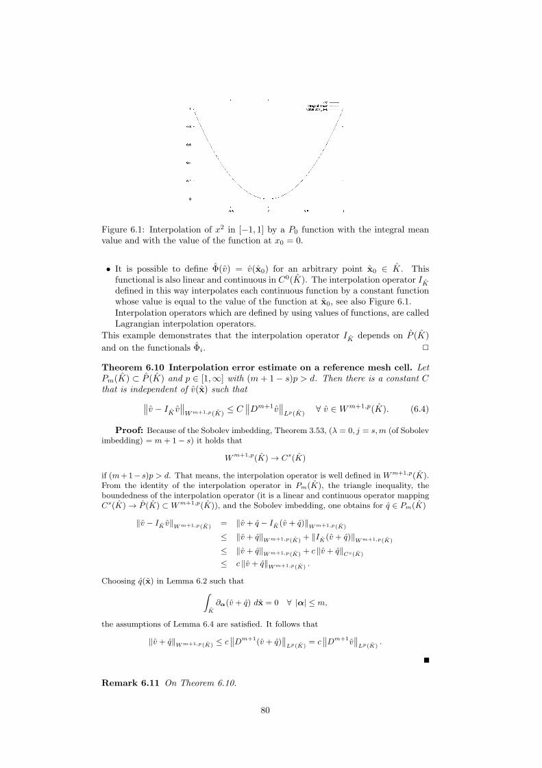
Figure 6.1: Interpolation of x2 in [−1, 1] by a P0 function with the integral meanvalue and with the value of the function at x0 = 0.

• It is possible to define Φ(v) = v(x0) for an arbitrary point x0 ∈ K. Thisfunctional is also linear and continuous in C0(K). The interpolation operator IKdefined in this way interpolates each continuous function by a constant functionwhose value is equal to the value of the function at x0, see also Figure 6.1.Interpolation operators which are defined by using values of functions, are calledLagrangian interpolation operators.

This example demonstrates that the interpolation operator IK depends on P (K)

and on the functionals Φi.

Theorem 6.10 Interpolation error estimate on a reference mesh cell. LetPm(K) ⊂ P (K) and p ∈ [1,∞] with (m+ 1− s)p > d. Then there is a constant Cthat is independent of v(x) such that

∥∥v − IK v

∥∥Wm+1,p(K)

≤ C∥∥Dm+1v

∥∥Lp(K)

∀ v ∈Wm+1,p(K). (6.4)

Proof: Because of the Sobolev imbedding, Theorem 3.53, (λ = 0, j = s,m (of Sobolevimbedding) = m+ 1− s) it holds that

Wm+1,p(K) → Cs(K)

if (m+1− s)p > d. That means, the interpolation operator is well defined in Wm+1,p(K).From the identity of the interpolation operator in Pm(K), the triangle inequality, theboundedness of the interpolation operator (it is a linear and continuous operator mappingCs(K) → P (K) ⊂ Wm+1,p(K)), and the Sobolev imbedding, one obtains for q ∈ Pm(K)

‖v − IK v‖Wm+1,p(K)

= ‖v + q − IK(v + q)‖Wm+1,p(K)

≤ ‖v + q‖Wm+1,p(K) + ‖IK(v + q)‖Wm+1,p(K)

≤ ‖v + q‖Wm+1,p(K) + c ‖v + q‖Cs(K)

≤ c ‖v + q‖Wm+1,p(K) .

Choosing q(x) in Lemma 6.2 such that

∫

K

∂α(v + q) dx = 0 ∀ |α| ≤ m,

the assumptions of Lemma 6.4 are satisfied. It follows that

‖v + q‖Wm+1,p(K) ≤ c∥∥Dm+1(v + q)

∥∥Lp(K)

= c∥∥Dm+1v

∥∥Lp(K)

.

Remark 6.11 On Theorem 6.10.

80

• One can construct examples which show that the Sobolev imbedding is not validif (m+ 1− s)p > d is not satisfied. In the case (m+ 1− s)p ≤ d, the statementof Theorem 6.10 is not true.Consider the interpolation of continuous functions (s = 0) with piecewise linearelements (m = 1) in Sobolev spaces that are also Hilbert spaces (p = 2). Then(m+1−s)p = 4 and it follows that the theorem can be applied only for d ∈ 2, 3.For piecewise constant finite elements, the statement of the theorem is true onlyfor d = 1.

• The theorem requires only that Pm(K) ⊂ P (K). This requirement does notexclude that P (K) contains polynomials of higher degree, too. However, thisproperty is not utilized and also not needed if the other assumptions of thetheorem are satisfied.

Remark 6.12 Assumptions on the triangulation. For deriving the interpolationerror estimate for arbitrary mesh cells K, and finally for the finite element space,one has to study the properties of the affine mapping from K to K and of the backmapping.

Consider an affine family of finite elements whose mesh cells are generated byaffine mappings

FK x = Bx+ b,

where B is a non-singular d× d matrix and b is a d vector.Let hK be the diameter of K = FK(K), i.e., the largest distance of two points

that are contained in K. The images K = FK(K) are assumed to satisfy thefollowing conditions:

• K ⊂ Rd is contained in a ball of radius CRhK ,

• K contains a ball of radius C−1R hK ,

where the constant CR is independent of K. Hence, it follows for all K that

radius of circumcircle

radius of inscribed circle≤ C2

R.

A triangulation with this property is called a quasi-uniform triangulation.

Lemma 6.13 Estimates of matrix norms. For each matrix norm ‖·‖ one hasthe estimates

‖B‖ ≤ chK ,∥∥B−1

∥∥ ≤ ch−1

K ,

where the constants depend on the matrix norm and on CR.

Proof: Since K is a Lipschitz domain with polyhedral boundary, it contains a ballB(x0, r) with x0 ∈ K and some r > 0. Hence, x0 + y ∈ K for all ‖y‖2 = r. It follows thatthe images

x0 = Bx0 + b, x = B(x0 + y) + b = x0 +By

are contained in K. Since the triangulation is assumed to be quasi-uniform, one obtainsfor all y

‖By‖2 = ‖x− x0‖2 ≤ CRhK .

Now, it holds for the spectral norm that

‖B‖2 = supz 6=0

‖Bz‖2‖z‖2

=1

rsup

‖z‖2=r

‖Bz‖2 ≤CR

rhK .

An estimate of this form, with a possible different constant, holds also for all other matrixnorms since all matrix norms are equivalent.

The estimate for∥∥B−1

∥∥ proceeds in the same way with interchanging the roles of K

and K.

81

Theorem 6.14 Local interpolation estimate. Let an affine family of finiteelements be given by its reference cell K, the functionals Φi, and a space ofpolynomials P (K). Let all assumptions of Theorem 6.10 be satisfied. Then, for allv ∈Wm+1,p(K) there is a constant C, which is independent of v(x) such that

∥∥Dk(v − IKv)

∥∥Lp(K)

≤ Chm+1−kK

∥∥Dm+1v

∥∥Lp(K)

, k ≤ m+ 1. (6.5)

Proof: The idea of the proof consists in transforming left hand side of (6.5) to thereference cell, using the interpolation estimate on the reference cell and transforming back.

i). Denote the elements of the matrices B and B−1 by bij and b(−1)ij , respectively.

Since ‖B‖∞ = maxi,j |bij | is also a matrix norm, it holds that

|bij | ≤ ChK ,∣∣∣b

(−1)ij

∣∣∣ ≤ Ch−1

K . (6.6)

Using element-wise estimates for the matrix B (Leibniz formula for determinants), oneobtains

|detB| ≤ ChdK ,

∣∣detB−1

∣∣ ≤ Ch−d

K . (6.7)

ii). The next step consists in proving that the transformed interpolation operator isequal to the natural interpolation operator on K. The latter one is given by

IKv =

N∑

i=1

ΦK,i(v)φK,i, (6.8)

where φK,i is the basis of the space

P (K) = p : K → R : p = p F−1K , p ∈ P (K),

which satisfies ΦK,i(φK,j) = δij . The functionals are defined by

ΦK,i(v) = Φi(v FK)

Hence, it follows with v = φj F−1K from the condition on the local basis on K that

ΦK,i(φj F−1K ) = Φi(φj) = δij ,

i.e., the local basis on K is given by φK,j = φj F−1K . Using (6.8), one gets

IK v =

N∑

i=1

Φi(v)φi =

N∑

i=1

ΦK,i(v F−1K

︸ ︷︷ ︸

=v

) φK,i FK =

(N∑

i=1

ΦK,i(v)φK,i

)

FK

= IKv FK .

Hence, IK v is transformed correctly.iii). One obtains with the chain rule

∂v(x)

∂xi=

d∑

j=1

∂v(x)

∂xjb(−1)ji ,

∂v(x)

∂xi=

d∑

j=1

∂v(x)

∂xjbji.

It follows with (6.6) that (with each derivative one obtains an additional factor of B orB−1, respectively)

∥∥∥D

kxv(x)

∥∥∥2≤ Ch−k

K

∥∥∥D

kxv(x)

∥∥∥2,∥∥∥D

kxv(x)

∥∥∥2≤ Chk

K

∥∥∥D

kxv(x)

∥∥∥2.

One gets with (6.7)∫

K

∥∥∥D

kxv(x)

∥∥∥

p

2dx ≤ Ch−kp

K |detB|

∫

K

∥∥∥D

kxv(x)

∥∥∥

p

2dx ≤ Ch−kp+d

K

∫

K

∥∥∥D

kxv(x)

∥∥∥

p

2dx

and∫

K

∥∥∥D

kxv(x)

∥∥∥

p

2dx ≤ Chkp

K

∣∣detB−1

∣∣

∫

K

∥∥∥D

kxv(x)

∥∥∥

p

2dx ≤ Chkp−d

K

∫

K

∥∥∥D

kxv(x)

∥∥∥

p

2dx.

82

Using now the interpolation estimate on the reference cell (6.4) yields

∥∥∥D

kx(v − IK v)

∥∥∥

p

Lp(K)≤ C

∥∥Dm+1

xv∥∥p

Lp(K), 0 ≤ k ≤ m+ 1.

It follows that∥∥∥D

kx(v − IKv)

∥∥∥

p

Lp(K)≤ Ch−kp+d

K

∥∥∥D

kx(v − IK v)

∥∥∥

p

Lp(K)

≤ Ch−kp+dK

∥∥Dm+1

xv∥∥p

Lp(K)

≤ Ch(m+1−k)pK

∥∥Dm+1

x v∥∥p

Lp(K).

Taking the p-th root proves the statement of the theorem.

Remark 6.15 On estimate (6.5).

• Note that the power of hK does not depend on p and d.• Consider a quasi-uniform triangulation and define

h = maxK∈T h

hK.

Then, one obtains by summing over all mesh cells an interpolation estimate forthe global finite element space

∥∥Dk(v − Ihv)

∥∥Lp(Ω)

=

∑

K∈T h

∥∥Dk(v − IKv)

∥∥p

Lp(K)

1/p

≤

∑

K∈T h

ch(m+1−k)pK

∥∥Dm+1v

∥∥p

Lp(K)

1/p

≤ ch(m+1−k)∥∥Dm+1v

∥∥Lp(Ω)

. (6.9)

For linear finite elements P1 (m = 1) it is, in particular,

‖v − Ihv‖Lp(Ω) ≤ ch2∥∥D2v

∥∥Lp(Ω)

, ‖∇(v − Ihv)‖Lp(Ω) ≤ ch∥∥D2v

∥∥Lp(Ω)

,

if v ∈W 2,p(Ω).

Corollary 6.16 Finite element error estimate. Let u(x) be the solution of themodel problem (4.9) with u ∈ Hm+1(Ω) and let uh(x) be the solution of the corre-sponding finite element problem. Consider a family of quasi-uniform triangulationsand let the finite element spaces V h contain polynomials of degree m. Then, thefollowing finite element error estimate holds

∥∥∇(u− uh)

∥∥L2(Ω)

≤ chm∥∥Dm+1u

∥∥L2(Ω)

= chm |u|Hm+1(Ω) . (6.10)

Proof: The statement follows by combining Lemma 4.13 (for V = H10 (Ω)) and (6.9)

∥∥∥∇(u− uh)

∥∥∥L2(Ω)

≤ infvh∈V h

∥∥∥∇(u− vh)

∥∥∥L2(Ω)

≤ ‖∇(u− Ihu)‖L2(Ω) ≤ chm |u|Hm+1(Ω) .

Remark 6.17 To (6.10). Note that Lemma 4.13 provides only information aboutthe error in the norm on the left-hand side of (6.10), but not in other norms.

83

6.2 Inverse Estimate

Remark 6.18 On inverse estimates. The approach for proving interpolation errorestimates can be uses also to prove so-called inverse estimates. In contrast tointerpolation error estimates, a norm of a higher order derivative of a finite elementfunction will be estimated by a norm of a lower order derivative of this function.One obtains as penalty a factor with negative powers of the diameter of the meshcell.

Theorem 6.19 Inverse estimate. Let 0 ≤ k ≤ l be natural numbers and letp, q ∈ [1,∞]. Then there is a constant Cinv, which depends only on k, l, p, q, K, P (K)such that

∥∥Dlvh

∥∥Lq(K)

≤ Cinvh(k−l)−d(p−1−q−1)K

∥∥Dkvh

∥∥Lp(K)

∀ vh ∈ P (K). (6.11)

Proof: In the first step, (6.11) is shown for hK = 1 and k = 0 on the reference meshcell. Since all norms are equivalent in finite dimensional spaces, one obtains

∥∥∥D

lvh∥∥∥Lq(K)

≤∥∥∥v

h∥∥∥W l,q(K)

≤ C∥∥∥v

h∥∥∥Lp(K)

∀ vh ∈ P (K).

If k > 0, then one sets

P (K) =

∂αvh : vh ∈ P (K), |α| = k

,

which is also a space consisting of polynomials. The application of the first estimate ofthe proof to P (K) gives

∥∥∥D

lvh∥∥∥Lq(K)

=∑

|α|=k

∥∥∥D

l−k(

∂αvh)∥∥∥Lq(K)

≤ C∑

|α|=k

∥∥∥∂αv

h∥∥∥Lp(K)

= C∥∥∥D

kvh∥∥∥Lp(K)

.

This estimate is transformed to an arbitrary mesh cell K analogously as for the interpo-lation error estimates. From the estimates for the transformations, one obtains

∥∥∥D

lvh∥∥∥Lq(K)

≤ Ch−l+d/qK

∥∥∥D

lvh∥∥∥Lq(K)

≤ Ch−l+d/qK

∥∥∥D

kvh∥∥∥Lp(K)

≤ Cinvhk−l+d/q−d/pK

∥∥∥D

kvh∥∥∥Lp(K)

.

Remark 6.20 On the proof. The crucial point in the proof was the equivalence ofall norms in finite dimensional spaces. Such a property does not exist in infinitedimensional spaces.

Corollary 6.21 Global inverse estimate. Let p = q and let T h be a regulartriangulation of Ω, then

∥∥Dlvh

∥∥Lp,h(Ω)

≤ Cinvhk−l∥∥Dkvh

∥∥Lp,h(Ω)

,

where

‖·‖Lp,h(Ω) =

∑

K∈T h

‖·‖pLp(K)

1/p

.

Remark 6.22 On ‖·‖Lp,h(Ω). The cell wise definition of the norm is importantfor l ≥ 2 since in this case finite element functions generally do not possess theregularity for the global norm to be well defined. It is also important for l ≥ 1 andnon-conforming finite element functions.

84

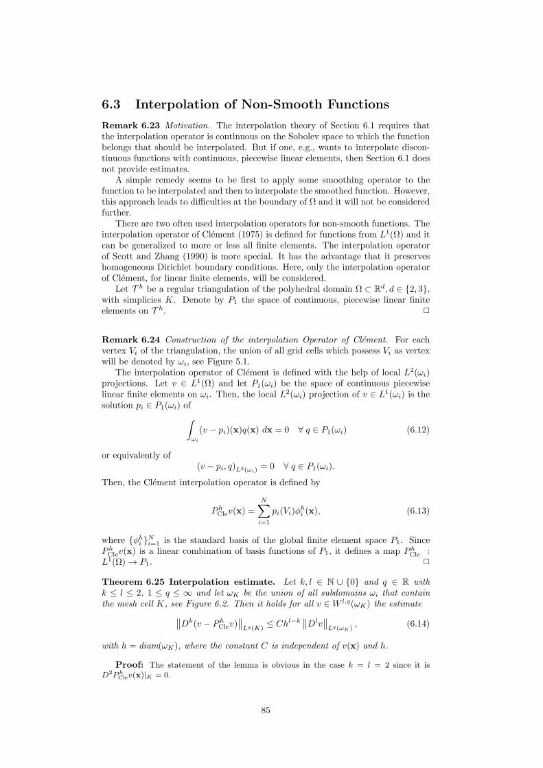
6.3 Interpolation of Non-Smooth Functions

Remark 6.23 Motivation. The interpolation theory of Section 6.1 requires thatthe interpolation operator is continuous on the Sobolev space to which the functionbelongs that should be interpolated. But if one, e.g., wants to interpolate discon-tinuous functions with continuous, piecewise linear elements, then Section 6.1 doesnot provide estimates.

A simple remedy seems to be first to apply some smoothing operator to thefunction to be interpolated and then to interpolate the smoothed function. However,this approach leads to difficulties at the boundary of Ω and it will not be consideredfurther.

There are two often used interpolation operators for non-smooth functions. Theinterpolation operator of Clement (1975) is defined for functions from L1(Ω) and itcan be generalized to more or less all finite elements. The interpolation operatorof Scott and Zhang (1990) is more special. It has the advantage that it preserveshomogeneous Dirichlet boundary conditions. Here, only the interpolation operatorof Clement, for linear finite elements, will be considered.

Let T h be a regular triangulation of the polyhedral domain Ω ⊂ Rd, d ∈ 2, 3,

with simplicies K. Denote by P1 the space of continuous, piecewise linear finiteelements on T h.

Remark 6.24 Construction of the interpolation Operator of Clement. For eachvertex Vi of the triangulation, the union of all grid cells which possess Vi as vertexwill be denoted by ωi, see Figure 5.1.

The interpolation operator of Clement is defined with the help of local L2(ωi)projections. Let v ∈ L1(Ω) and let P1(ωi) be the space of continuous piecewiselinear finite elements on ωi. Then, the local L2(ωi) projection of v ∈ L1(ωi) is thesolution pi ∈ P1(ωi) of

∫

ωi

(v − pi)(x)q(x) dx = 0 ∀ q ∈ P1(ωi) (6.12)

or equivalently of(v − pi, q)L2(ωi)

= 0 ∀ q ∈ P1(ωi).

Then, the Clement interpolation operator is defined by

PhClev(x) =

N∑

i=1

pi(Vi)φhi (x), (6.13)

where φhi Ni=1 is the standard basis of the global finite element space P1. Since

PhClev(x) is a linear combination of basis functions of P1, it defines a map Ph

Cle :L1(Ω) → P1.

Theorem 6.25 Interpolation estimate. Let k, l ∈ N ∪ 0 and q ∈ R withk ≤ l ≤ 2, 1 ≤ q ≤ ∞ and let ωK be the union of all subdomains ωi that containthe mesh cell K, see Figure 6.2. Then it holds for all v ∈W l,q(ωK) the estimate

∥∥Dk(v − Ph

Clev)∥∥Lq(K)

≤ Chl−k∥∥Dlv

∥∥Lq(ωK)

, (6.14)

with h = diam(ωK), where the constant C is independent of v(x) and h.

Proof: The statement of the lemma is obvious in the case k = l = 2 since it isD2Ph

Clev(x)|K = 0.

85

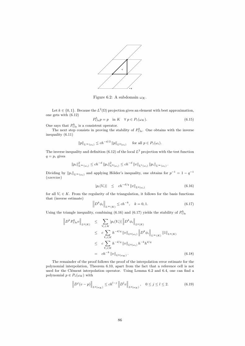
Figure 6.2: A subdomain ωK .

Let k ∈ 0, 1. Because the L2(Ω) projection gives an element with best approximation,one gets with (6.12)

PhClep = p in K ∀ p ∈ P1(ωK). (6.15)

One says that PhCle is a consistent operator.

The next step consists in proving the stability of PhCle. One obtains with the inverse

inequality (6.11)

‖p‖L∞(ωi)≤ ch−d/2 ‖p‖L2(ωi)

for all p ∈ P1(ωi).

The inverse inequality and definition (6.12) of the local L2 projection with the test functionq = pi gives

‖pi‖2L∞(ωi)

≤ ch−d ‖pi‖2L2(ωi)

≤ ch−d ‖v‖L1(ωi)‖pi‖L∞(ωi)

.

Dividing by ‖pi‖L∞(ωi)and applying Holder’s inequality, one obtains for p−1 = 1 − q−1

(exercise)

|pi(Vi)| ≤ ch−d/q ‖v‖Lq(ωi)(6.16)

for all Vi ∈ K. From the regularity of the triangulation, it follows for the basis functionsthat (inverse estimate)

∥∥∥D

kφi

∥∥∥L∞(K)

≤ ch−k, k = 0, 1. (6.17)

Using the triangle inequality, combining (6.16) and (6.17) yields the stability of PhCle

∥∥∥D

kPhClev

∥∥∥Lq(K)

≤∑

Vi∈K

|pi(Vi)|∥∥∥D

kφi

∥∥∥Lq(K)

≤ c∑

Vi∈K

h−d/q ‖v‖Lq(ωi)

∥∥∥D

kφi

∥∥∥L∞(K)

‖1‖Lq(K)

≤ c∑

Vi∈K

h−d/q ‖v‖Lq(ωi)h−khd/q

= ch−k ‖v‖Lq(ωK) . (6.18)

The remainder of the proof follows the proof of the interpolation error estimate for thepolynomial interpolation, Theorem 6.10, apart from the fact that a reference cell is notused for the Clement interpolation operator. Using Lemma 6.2 and 6.4, one can find apolynomial p ∈ P1(ωK) with

∥∥∥D

j(v − p)∥∥∥Lq(ωK)

≤ chl−j∥∥∥D

lv∥∥∥Lq(ωK)

, 0 ≤ j ≤ l ≤ 2. (6.19)

86

With (6.15), the triangle inequality, ‖·‖Lq(K) ≤ ‖·‖Lq(ωK), (6.18), and (6.19), one obtains

∥∥∥D

k(

v − PhClev

)∥∥∥Lq(K)

=∥∥∥D

k(

v − p+ PhClep− Ph

Clev)∥∥∥Lq(K)

≤∥∥∥D

k(v − p)∥∥∥Lq(K)

+∥∥∥D

kPhCle(v − p)

∥∥∥Lq(K)

≤∥∥∥D

k(v − p)∥∥∥Lq(ωK)

+ ch−k ‖v − p‖Lq(ωK)

≤ chl−k∥∥∥D

lv∥∥∥Lq(ωK)

+ ch−khl∥∥∥D

lv∥∥∥Lq(ωK)

= chl−k∥∥∥D

lv∥∥∥Lq(ωK)

.

Remark 6.26 Uniform meshes.

• If all mesh cells in ωK are of the same size, then one can replace h by hK in theinterpolation error estimate (6.14). This property is given in many cases.

• If one assumes that the number of mesh cells in ωK is bounded uniformly for allconsidered triangulations, the global interpolation estimate

∥∥Dk(v − Ph

Clev)∥∥Lq(Ω)

≤ Chl−k∥∥Dlv

∥∥Lq(Ω)

, 0 ≤ k ≤ l ≤ 2,

follows directly from (6.14).

87