sobolev spaces. elliptic equations - institut camille...
TRANSCRIPT

Sobolev spaces. Elliptic equations
Petru Mironescu
December 2010
0 Introduction
The purpose of these notes is to introduce some basic functional and harmonicanalysis tools (Sobolev spaces, singular integrals) and to explain how thesetools are used in the study of elliptic partial differential equations. In a lastpart, we will introduce some basic variational methods, applied to existenceof solutions of semi linear elliptic problems.
Many books and papers are at the origin of these notes:
Sobolev spacesRobert A. Adams, John J.F. Fournier: Sobolev Spaces. 2nd ed, Elsevier
2003Haım Brezis, Analyse fonctionnelle. Theorie et applications, Masson 1983Michel Willem, Analyse fonctionnelle elementaire, Cassini 2003Louis Nirenberg, On elliptic partial differential equations, Ann. Sc. Norm.
Sup. Pisa 13 (1959), p. 116-162Haım Brezis, Augusto C. Ponce, Kato’s inequality up to the boundary,
Comm. Contemp. Math. 10 (2008), p. 1217–1241Lars Hormander, The Analysis of Linear Partial Differential Operators I,
Springer, 1990Richard Courant, David Hilbert, Methods of Modern Mathematical Physics,
II, Interscience, 1962Elliott H. Lieb, Michael Loss, Analysis, 2nd edition, American Mathe-
matical Society, 2001Moshe Marcus, Victor Mizel, Every superposition operator mapping one
Sobolev space into another is continuous, J. Funct. Anal. 33 (1979), no. 2,217–229
Xavier Lamy showed me a proof, much simpler than the one I initiallyfound, of Lemma 1.98. I included his proof in the text
1

Singular integralsElias Stein, Harmonic analysis: real-variable methods, orthogonality, and
oscillatory integrals, Princeton University Press, 1993Elias Stein, Guido Weiss, Introduction to Fourier analysis on Euclidean
spaces, Princeton University Press, 1971Lawrence Evans, Ronald Gariepy, Measure theory and fine properties of
functions, CRC Press, 1992
Linear elliptic equationsDavid Gilbarg, Neil S. Trudinger, Elliptic partial differential equations of
second order, 4th ed., Springer 2001Quin Han, Fanghua Lin, Elliptic Partial Differential Equations, American
Mathematical Society 2000
0.1 Notations
a) If 1 ≤ p ≤ ∞, p′ stands for the conjugate of p (thus1
p+
1
p′= 1)
b) N is the space dimension
c) RN+ = x ∈ RN ;xN > 0, RN
− = x ∈ RN ;xN < 0
d) Ω is an open set in RN . Unless stated otherwise, Ω is supposed connected(i. e., Ω is a domain)
e) α, β stand for multi-indices in NN . We let |α| =N∑j=1
|αj|
f) |A| is the (usually Lebesgue, sometimes Hausdorff) measure of A
g)
denotes the average integral:
A
f =1
|A|
ˆA
f
h) | | stands for the standard Euclidean norm. E. g., |∇u| =
√∑(∂u
∂xj
)2
i) ρ is a standard mollifier, i. e. a map s. t. ρ ∈ C∞c (RN ;R), ρ ≥ 0,ˆρ = 1, supp ρ ⊂ B(0, 1)
j) ν stands for the unit outward normal at the boundary of a smooth domainΩ
2

k) A b Ω means that A is a compact subset of the open set Ω
l) In principle, K is always a compact set, but I may forget this here andthere and let K also denote a constant. Also in principle, ω is an opensubset of Ω
m) The subscript loc stands for the local version of the spaces we consider.This will not be defined each time, so that we content ourselves to give,once for all, an example:
W 1,1loc (Ω) = u ∈ L1(Ω);u|K ∈ L1,∇u|K ∈ L1,∀ K c Ω
n) We let ωN denote the volume of the (Euclidean) unit ball in RN , and σNdenote the (H N−1 dimensional) measure of the (Euclidean) unit sphere.Recall that these two quantities are related by σN = NωN
o) M is the set of measurable functions
p) If C is a ball in RN (with respect to some norm), then we let C∗ denote thecube having the same center as C and twice the same radius. Similarly,C∗∗ has four times the radius of C
1 Sobolev spaces
1.1 Motivation
Let u solve the problem −∆u = f in Ω
u = 0 on ∂Ω, (1.1)
aka as the Dirichlet problem for the Poisson equation. Assume everythingsmooth. Multiply the first equation by v ∈ C2(Ω) s. t. v = 0 on ∂Ω andintegrate once by parts (i. e., use the first Green formula). We find that
ˆΩ
∇u · ∇v −ˆ∂Ω
∂u
∂νv =
ˆΩ
fv,
i. e., ˆΩ
∇u · ∇v −ˆ
Ω
fv = 0, ∀ v ∈ X,
3

where X := v ∈ C2(Ω); v = 0 on ∂Ω. Formally, this is the same asDJ(u) = 0, where J : X → R is given by
J(u) :=1
2
ˆΩ
|∇u|2 −ˆ
Ω
fu.
This suggests the following strategy intended to solve (1.1): minimize J inX. Then the minimizer should solve (1.1). Good news: if u is a minimizer,then it is indeed the solution of (1.1). Problem with that: the minimumneed not exist. A first reason is that if we take a minimizing sequence (i.e., a sequence such that J(un) → min), then there is no reason to obtainsome u ∈ X s. t. un → u (whatever the sense we give to this convergence).Actually, Weierstrass showed that, if f is continuous, then there may not bea minimum point of J in X. A way to overcome this difficulty is to replaceX by a larger space, where the minimum is attained (but not necessarily bysome u ∈ X). It turns out that the good candidate is the closure Y of X for
the norm u 7→(ˆ
Ω
|∇u|2)1/2
. As we will see later, this is a Sobolev space.
Sobolev spaces are useful even when (1.1) does have a solution in X. Indeed,existence can be proved as follows: start by minimizing J in Y (this is alwayspossible), then prove that u ∈ X (this requires extra assumptions on f , andthe proof of such type of results is the purpose of regularity theory). This isHilbert’s strategy.
1.2 Distributions
Distributions were formalized by Schwartz, but predecessors of this theoryappear already in the works of Leray and Sobolev.
1.1 Definition. Let Ω ⊂ RN be an open set. A distribution on Ω is a linearfunctional u on C∞c (Ω) which is continuous in the following sense: for eachcompact K b Ω, there is a constant C and an integer k s. t.
|u(ϕ)| ≤ C∑|α|≤k
sup |∂αϕ|, ∀ ϕ ∈ C∞c (Ω) s. t. supp ϕ ⊂ K.
The vector space of the distributions is denoted D ′(Ω).
1.2 Example. A continuous function u defines a distribution, still denoted u,
through the formula u(ϕ) =
ˆΩ
ϕ. More generally, one can replace continuous
by measurable and integrable on compacts. In this case, we may take k = 0
and C =
ˆK
|u|.
4

There is a good reason to keep the notation u for the above distribution
1.3 Proposition (Localisation principle). Let u, v ∈ L1loc(Ω). Then u = v
a. e. iff the distributions defined by u and v are equal.In other words, one can identify u with the associated distribution.
Proof. The only if part is clear. For the if part, we rely on the following factthat we will prove later
1.4 Proposition. Let ρ be a standard mollifier. Let f ∈ L1loc(Ω). Then
f ∗ ρε → f a. e. as ε→ 0.
1.5 Remark. Note that f ∗ ρε is defined in Ωε = x ∈ Ω; dist (x, ∂Ω) > ε.Thus, for each x ∈ Ω, f ∗ρε(x) is well defined for small ε (smallness dependingon ε).
Back to the proof of the localisation principle. With f = u− v, we haveˆfϕ = 0 for each ϕ ∈ C∞c (Ω). In particular, f ∗ ρε = 0 for each ε. We
conclude by letting ε→ 0.
1.6 Example. If a ∈ Ω, then δa(ϕ) = ϕ(a) is a distribution (the Dirac massat a). Indeed, we may take k = 0 and C = 1. When a = 0, we write δ ratherthan δ0.
1.7 Example. If Σ is a k-dimensional submanifold of Ω, then δΣ(ϕ) =ˆΣ
ϕdH k is a distribution (the Dirac mass on Σ). Indeed, we may take
k = 0 and C the Hausdorff measure of Σ ∩K.More generally, we may consider the distribution fH kxΣ, where f is locallyintegrable (with respect to Hk) on Σ. This distribution acts through the
formula ϕ 7→ˆ
Σ
fϕ dH k.
1.8 Example. All the above examples are special cases of measures: if µis a locally finite Borel measure , then µ defines a distribution through the
formula µ(ϕ) =
ˆΩ
ϕ. (Take k = 0 and C = |µ|(K).)
1.9 Exercise. It is not always possible to take k = 0. For example, letu(ϕ) = ϕ′(0) (assuming that 0 ∈ Ω and N = 1). Then u ∈ D ′(Ω), but it isnot possible to take k = 0 when, say, K is a closed interval centered at theorigin.Hint: consider ϕ(nx) for a fixed ϕ.
The next result identifies (positive) measures.
5

1.10 Proposition. Let u ∈ D ′(Ω). Then the following are equivalent:
(i) u is ”positive”, in the sense that u(ϕ) ≥ 0 if ϕ ∈ C∞c (Ω) and ϕ ≥ 0
(ii) There is some positive Radon measure µ s. t. u(ϕ) =
ˆϕdµ, ∀ ϕ ∈
C∞c (Ω).
If these conditions are satisfied, we write u ≥ 0.
Proof. The implication (ii)=⇒(i) is clear. Conversely, let K b Ω and letψ ∈ C∞c (Ω) be s. t. 0 ≤ ψ ≤ 1 and ψ ≡ 1 in K. If ϕ ∈ C∞c (K), then
−‖ϕ‖L∞u(ψ) ≤ u(ϕ) ≤ ‖ϕ‖L∞u(ψ),
so that |u(ϕ)| ≤ C(K)‖ϕ‖L∞ , ∀ ϕ ∈ C∞c (K). We find that u has a linearpositive continuous extension to Cc(Ω). We conclude via the Riesz represen-tation theorem.
When u ∈ C1(Ω), we have ∂ju(ϕ) = −u(∂jϕ) (this is obtained by inte-gration by parts). This suggests the following
1.11 Definition. If u ∈ D ′(Ω), we define ∂ju through the formula ∂ju(ϕ) =−u(∂jϕ). More generally, ∂αu(ϕ) = (−1)|α|u(∂αϕ). This is still a distribu-tion.If P (∂) =
∑aα∂
α, then we define (P (∂)u)(ϕ) =∑
(−1)|α|aαu(∂αϕ).
In the same vein, we define, for u ∈ D ′(Ω) and a ∈ C∞(Ω), the distributionau by (au)(ϕ) = u(aϕ).
Two points are of interest: the result is still a distribution, and these def-initions coincide with the usual ones when u is smooth enough. For example,when u ∈ C1, we have ”old ∂ju=new ∂ju”. When we want to emphasizesuch an equality, we write ∂j,pu = ∂j,du (p stands for point derivative, d fordistributional derivative).
1.12 Remark. When there is a possible doubt, we let the subscript p standfor point quantities, and d for distributional ones.
1.13 Exercise. If a ∈ C∞(Ω) and u ∈ D ′(Ω), we have the following Leibnizrule
∂α(au) =∑β≤α
α!
β!(α− β)!∂βa∂α−βu.
1.14 Exercise. If f(x) = |x| (in R), then f ′ = sgn.
6

1.15 Exercise. If f(x) =
1, if x > 0
0, if x ≤ 0(in R), then f ′ = δ.
1.16 Exercise. Let Ω1, Ω2 be smooth open sets s. t. Ω1 ∩ Ω2 = ∅ andΩ1∩Ω2 = Σ, with Σ smooth hypersurface. Let ui ∈ C1(Ωi∪Σ), i = 1, 2, and
set u =
u1, in Ω1
u2, in Ω2
. Then ∂ju = ∂ju1χΩ1 + ∂ju2χΩ2 + (u2 − u1)νjH kxΣ.
Here, ν is the normal to Σ directed from Ω1 to Ω2.
A slightly more involved result is the following
1.17 Proposition. Assume that N ≥ 2, 0 ∈ Ω. Let f ∈ C1(Ω\0) be suchthat ∇pu ∈ L1
loc(Ω). Then ∂j,pu = ∂j,du.
Proof. We have to prove that
ˆΩ
u∂jϕ = −ˆ
Ω
∂j,puϕ, ϕ ∈ C∞c (Ω). We drop
the subscript p. The key fact is that
ˆS(0,ε)
|u| dH N−1 = o(1) as ε → 0.
(This will imply u ∈ L1loc(Ω).) Assuming this for the moment, we argue as
followsˆΩ
u∂juϕ = limε→0
ˆΩ\B(0,ε)
∂juϕ = limε→0
(ˆS(0,ε)
νjuϕ−ˆ
Ω\B(0,ε)
u∂jϕ
)= − lim
ε→0
ˆΩ\B(0,ε)
u∂jϕ = −ˆ
Ω
u∂jϕ.
We now prove the key fact (and its consequence). Assume e. g., in what fol-lows, that B(0, 1) b Ω. We start by noting that (by dominated convergence)
limε→0
ˆB(0,1)\B(0,ε)
εN−1
|x|N−1|∇u| = 0.
We claim that ˆS(0,ε)
|u| ≤ CεN−1 +
ˆB(0,1)\B(0,ε)
εN−1
|x|N−1|∇u|.
This follows fromˆS(0,ε)
|u| = εN−1
ˆSN−1
|u(εω)| dH N−1
= εN−1
ˆSN−1
∣∣∣∣u(ω)−ˆ 1
ε
d
dr[u(rω)]
∣∣∣∣ dH N−1
≤ εN−1
ˆSN−1
|u| dH N−1 +
ˆΩ\B(0,ε)
εN−1
|x|N−1|∇u|.
7

Consequence: if K c Ω, thenˆK
|u| ≤ˆB(0,1)
|u|+ supK\B(0,1)
|u| ≤ sup0≤ε≤1
ˆS(0,ε)
|u|+ supK\B(0,1)
|u| <∞,
i. e., u ∈ L1loc(Ω).
In order to establish our next example, we need the following simple fact
1.18 Proposition (Delocalisation principle). If u = v on Ωi, i ∈ I, thenu = v on ∪Ωi.
Proof. Let Ω = ∪Ωi, ϕ ∈ C∞c (Ω) and ϕi be a finite partition of unity on supp
ϕ subordinated to the covering (Ωi). Then u(ϕ) =∑
u(ϕiϕ) =∑
v(ϕiϕ) =
v(ϕ).
1.19 Proposition. Let Σ be a k-dimensional submanifold of Ω (here, k ≤N − 2). Let u ∈ C1(Ω \ Σ) be such that ∇pu ∈ L1
loc(Ω). Then ∂j,pu = ∂j,du.Conversely, if ∂j,du ∈ L1
loc(Ω), then ∂j,pu ∈ L1loc(Ω).
Note that Proposition 1.17 is a special case (when k = 0) of the aboveresult.
Proof. We start with a special case, later referred as the standard case. We letΩ = BRN−k(0, 1)×(−1, 1)k, Σ = 0×(−1, 1)k and assume that u ∈ C1(Ω\Σ).Write a point in RN as x = (x′, x′′), with x′ ∈ RN−k, x′′ ∈ Rk. As in theproof of Proposition 1.17, we haveˆ
x∈Ω;|x′|=ε|u| ≤ CεN−k−1 +
ˆΩ
εN−k−1
|x′|N−k−1|∇u| → 0 as ε→ 0.
Consequently, we have u ∈ L1(Ω) andˆx∈Ω;|x′|≤ε
|u| = o(ε) as ε→ 0.
Let now ψ ∈ C∞(R;R) be s. t. ψ(t) =
1, if t ≥ 1
0, if t ≤ 1/2. For ϕ ∈ C∞c (Ω) we
have ˆΩ
u∂jϕ = limε→0
ˆΩ
uψ(|x′|/ε)∂jϕ = − limε→0
ˆΩ
∂j(uψ(|x′|/ε))ϕ
= −ˆ
Ω
∂juϕ− limε→0
ˆΩ
u∂j[ψ(|x′|/ε))]ϕ
= −ˆ
Ω
∂juϕ− limε→0
1
εO
(ˆx∈Ω;|x′|≤ε
|u|)
= −ˆ
Ω
∂juϕ.
8

We now turn to the general case. We cover Ω with a family (Ωi) of opensets s. t., for each i: either Ωi ∩ Σ = ∅, or there is a C1 diffeomorphismΦi : Ωi → Ω0 (here, Ω0 stands for the open set from the standard example)s. t. Φ(Σ∩Ωi) = 0×Rk. In view of the delocalisation principle, it sufficesto prove that ∂j,pu = ∂j,du in each Ωi. This equality is clear if Σ does notmeet Ωi. Otherwise, let ϕ ∈ C∞c (Ω) be s. t. supp ϕ ⊂ Ωi. Then
ˆΩi
u∂jϕ = limε→0
uψ(|(Φi(x))′|/ε)∂jϕ = − limε→0
ˆΩi
∂j(uψ(|(Φi(x))′|/ε))ϕ
= −ˆ
Ωi
uϕ− limε→0
ˆΩi
u∂j(ψ(|(Φi(x))′|/ε))ϕ = −ˆ
Ωi
uϕ.
Here, we use the fact that |∂j(ψ(|(Φi(x))′|/ε))| ≤ C/ε combined withˆx∈Ωi;|(Φi(x))′|≤ε
|u| ≤ C
ˆx∈Ω0;|x′|≤ε
|u Φ−1i | = o(ε) as ε→ 0.
The last property is a consequence of the fact that u Φ−1i falls into the
standard case.We end with the converse: since u ∈ C1(Ω \ Σ), we have ∂j,pu = ∂j,du a. e.in Ω \ Σ. Since Σ is a null set, we find that ∂j,pu = ∂j,du a. e. in Ω, so that∂j,pu ∈ L1
loc.
Another useful operation (in addition to differentiation and multiplicationbe smooth functions) is convolution.
1.20 Definition. If u ∈ D ′(RN) and ϕ ∈ C∞c (RN), we set u ∗ ϕ(x) =u(ϕ(x− ·)).
One may prove the following
1.21 Proposition. We have u ∗ ϕ ∈ C∞ and ∂β+γ(u ∗ ϕ) = (∂βu) ∗ (∂γϕ).
Proof. The second property is trivial. We sketch the argument leading to thefirst one. The key fact is continuity, which is obtained as follows: if xn → x,then there is a fixed compact K s. t. supp ϕ(xn − ·) ⊂ K for each n. Since∂α(ϕ(xn − ·) − ϕ(x − ·)) → 0 uniformly in K, we find (using the definitionof a distribution) that u ∗ ϕ(xn)→ u ∗ ϕ(x). Similarly, we have
limt→0
u ∗ ϕ(x+ tej)− u ∗ ϕ(x)
t= u ∗ ∂jϕ(x).
By the key fact, the latter quantity is continuous in x. Thus u ∗ ϕ ∈ C1 and∂ju∗ϕ = u∗∂jϕ. We continue by induction on the number of derivatives.
9
1.22 Example. δ ∗ ϕ = δ.
Convolution can be considered in other settings (not only D ′(RN) vsC∞c (RN)), e. g., L1 vs Lp. We will come back to this later.
1.23 Exercise. A final point we discuss here is extension. If u ∈ D ′(Ω)and ω is an open subset of Ω, then we may restrict u to ω in the obviousway: we let u act on C∞c (ω). The converse is not always possible: givena distribution u on ω, it may not be the restriction of a distribution on Ω.Check the following: if ω = (0, 2) and Ω = R, there is no distribution on Ω
whose restriction to ω is u =∑
δ1/n.
1.3 First properties of Sobolev spaces
1.3.1 Definition
1.24 Definition. Let 1 ≤ p ≤ ∞. Then
W 1,p = W 1,p(Ω) = u ∈ Lp(Ω); ∂ju ∈ Lp(Ω).
We endow this vector space with the norm ‖u‖W 1,p = ‖u‖Lp +∑j
‖∂ju‖Lp .
When p <∞, another possible (equivalent) norm is
(‖u‖pLp +
∑j
‖∂ju‖pLp
)1/p
.
When p = 2, W k,2 is aka H1.
Note that Lp ⊂ L1loc, so that Lp functions are in D ′(Ω). Thus ∂ju makes
sense (as a distribution).
1.25 Example. Assume that Ω = BRN (0, 1). Let u(x) = |x|−α, whereα ∈ R. We claim that u ∈ W 1,p iff p(α + 1) < N .Indeed, to start with, we have u ∈ Lp iff pα < N . Next, we have |∇pu(x)| ∼|x|−α−1, so that ∇pu ∈ L1
loc if and only if α < N − 1. If α ≥ N − 1, then wecannot have ∇du ∈ L1
loc (in view of Proposition 1.19). Thus we cannot haveu ∈ W 1,p. If α < N − 1, then ∇pu = ∇du, so that ∇u ∈ Lp iff p(α+ 1) < N .We find that u ∈ W 1,p iff p(α + 1) < N .
1.3.2 W 1,∞ and Lip
1.26 Theorem. We have u ∈ W 1,∞ iff (possibly after redefining u on a nullset) u is bounded and there is some C > 0 s. t. (P) |u(x)− u(y)| ≤ C|x− y|
10

whenever [x, y] ⊂ Ω.In the special case where Ω is convex, this is the same as u bounded andLipschitz. In this case, ‖u‖W 1,∞ ∼ ‖u‖L∞ + |u|Lip.
1.27 Remark. In particular, the theorem asserts that u equals a. e. acontinuous function. We will write, here and there, ”u is continuous” as ashorthand for ”u is equal a. e. to a continuous function”.
Proof. Assume first that u ∈ W 1,∞. Then
|∇(u ∗ ρε)| = |(∇u) ∗ ρε)| ≤ ‖∇u‖L∞‖ρε‖L1 = ‖∇u‖L∞ .
We find that the family (u ∗ ρε) satisfies |u ∗ ρε| ≤ ‖u‖L∞ and (by the meanvalue theorem) condition (P ). By Arzela-Ascoli, we have (possibly afterextraction) u∗ρε → v uniformly on compacts. Clearly, the limit is continuous,bounded (since u is), and satisfies (P ). Since, on the other hand, we haveu ∗ ρε → u a. e., we proved the only if part.Conversely, by delocalisation we may assume Ω bounded and convex. We letas an exercise the fact that if (P ) holds, then u ∗ ρε is C-Lipschitz. Thus|∇(u ∗ ρε)| ≤ C. Thus the family (∇(u ∗ ρε)) is bounded in L∞ (and thus inL2). It is a standard fact in functional analysis that, under such assumptions,possibly after passing to a subsequence, we have ∇(u ∗ ρε) f in L2 forsome f s. t. |f | ≤ C. Using the definition of weak convergence, we find that∇du = f .On the way, we also proved norm equivalence when Ω is convex.
1.28 Exercise. Prove the ”standard fact” mentioned above, which amountsto: if fn, f ∈ L2(Ω) are s. t. |fn| ≤ C and fn f in L2, then |f | ≤ C a. e.(here, fn, f may be vector-valued).
Hint: compute
ˆ|f |>C
f · f|f |
.
1.29 Exercise. Let Ω = x ∈ R2 \ R−; 1 < |x| < 2 and u(reıθ) = θ,1 < r < 2, θ ∈ (−π, π). Prove that u ∈ W 1,∞, but u 6∈ Lip.
We will now see for the first time the role of the regularity of Ω. In viewof the above example, in general we do not have W 1,∞ = Lip. However,this holds under additional assumptions on Ω. A deep question that will besystematically overlooked in what follows is the one of minimal assumptionsthat make ”useful theorems” (embeddings, compactness, etc.) work. Mostof time, we will consider ”lazy assumptions” that make some rather simpleproofs work. For sharper results in this direction, the books of Adams andFournier, respectively Maz’ja, on Sobolev spaces, are good references.
11

1.30 Theorem. Assume that Ω is a bounded Lipschitz domain. Then W 1,∞ =Lip, and ‖u‖W 1,∞ ∼ ‖u‖L∞ + |u|Lip.
Proof. When Ω is Lipschitz, the geodesic distance dΩ in Ω is equivalent tothe Euclidean one. (Recall that dΩ(x, y) is the infimum of the length of allpolygonal lines connecting x to y. Such lines do exist, since Ω is a domain.)Clearly, the proof of Theorem 1.26 implies that ‖u‖W 1,∞ ≤ ‖u‖L∞ +N |u|Lip.Conversely, by the same theorem we have |u(x) − u(y)| ≤ ‖∇u‖L∞dΩ(x, y).We conclude using the fact that the geodesic distance is of the same orderas the Euclidean one.
1.31 Exercise. Prove the equivalence between geodesic and Euclidean dis-tance in Lipschitz bounded domains.Hint: cover Ω with balls which are: either contained in Ω, or chart domainson which ∂Ω can be straightened. Extract a finite covering, then considerthe Lebesgue number r associated to this covering. Estimate dΩ(x, y) byconsidering the cases |x− y| ≤ r and |x− y| > r.
1.3.3 1D
We assume, e. g., that 0 ∈ Ω and that Ω is an interval. The description ofSobolev spaces is basically a consequence of the following
1.32 Theorem. Let u, v ∈ L1loc(−1, 1). Then u′ = v iff there is some C s.
t. (possibly after redefining u on a null set) u(x) = C +
ˆ x
0
v(t) dt.
Proof. It is straightforward (by definition+Fubini) that u0(x) =
ˆ x
0
v(t) dt
satisfies u′0 = v. The conclusion follows from the next lemma.
1.33 Lemma. Let u ∈ D ′(Ω) (with Ω ⊂ R an interval). Then u′ = 0 iffu ∈ L1
loc and u = C a. e.
Proof. The if part is clear. Conversely, fix ϕ0 ∈ C∞c (Ω) s. t.
ˆϕ0 = 1. Let
ϕ ∈ C∞c (Ω) ans set ψ = ϕ −(ˆ
ϕ
)ϕ0. Then ψ has zero average, which
implies that ψ = ζ ′ for some ζ ∈ C∞c (Ω). We find that, with C = u(ϕ0), wehave
u(ϕ) =
ˆCϕ+ u(ψ) =
ˆCϕ− u′(ζ) =
ˆCϕ,
i. e., u = C in D ′(Ω). We conclude via the localisation principle.
12

1.34 Remark. From now on we identify maps with derivatives in L1loc with
their (existing and unique) continuous representative.
1.35 Corollary. If Ω is bounded, then W 1,p → C(Ω), with continuous em-bedding.
Proof. Inclusion is clear. Continuity follows from the closed graph theorem(since, as we will se later, W 1,p is a Banach space).
1.36 Corollary. Assume that u′ ∈ L1loc. Then u has a (usual) derivative u′p
a. e., and u′p = u′ a. e.
Proof. Let u′ = v. Then, for a. e. x ∈ Ω, we have (by the Lebesgue
differentiation theorem) u′p(x) = limh→0
ˆ x+h
x
v(t) dt
h= v(x).
1.37 Corollary. Lipschitz functions of one variable are differentiable a. e.
The next result is due to Lebesgue.
1.38 Theorem. Assume that u is bounded. Then u ∈ W 1,1 iff u is absolutelycontinuous.
Proof. Recall that absolutely continuity means: for each ε > 0, there is some
−∆ > 0 s. t. if (ai, bi) are disjoint intervals in Ω s. t.∑
(bi − ai) < −∆,
then∑|u(bi)− u(ai)| < ε.
The only if condition is a special case of Lebesgue’s lemma applied to
v = u′. This lemma asserts that if |A| < −∆, then
ˆA
|v| < ε (provided −∆
is sufficiently small). If we take A = ∪(ai, bi), then we recover the absolutecontinuity condition.
Conversely, if u is absolutely continuous (AC), then the following factsare easy to check and left as an exercise:
a) If u is AC, then u is continuous and has bounded variation
b) If we let u = u1−u2 be the Jordan decomposition of u (i. e., u1(x) =∨x
0 u,u2 = u1 − u; these functions are non decreasing), then u1, u2 are AC
c) Write each ui, i = 1, 2, as ui(x) = Ci + µi((−∞, x)) for appropriate mea-sures µi. (This is possible since each ui is continuous and non decreasing.)Then µi has the property that if ω is an open set and |ω| < −∆, thenµi(ω) < ε
13

d) Consequently, if ω is a Borel null set, then µi(ω) = 0
e) By the Radon-Nikodym theorem, there is some vi ∈ L1 s. t. ui(x) =
Di +
ˆ x
0
vi(t) dt
f) This implies at once that u′ = v1 − v2 ∈ L1.
1.39 Theorem. The following are equivalent, when 1 ≤ p <∞:
a) u = 0 on ∂Ω
b) u belongs to the closure, in W 1,p, of C∞c (Ω)
c) the extension of u with the value 0 outside Ω is in W 1,p(R).
Proof. We assume that Ω is bounded, e. g., Ω = (−1, 1). The proofs have tobe adapted to the other cases (Ω is a half line or R).
(a) implies (c). Let ˜ denote the extension with the value zero outside
Ω. Let v = u′. Then
ˆ 1
−1
v = 0. We find that u(x) =
ˆ x
−1
v(t) dt. This implies
(c).(c) implies (b). Let w = u′. We clearly have w = 0 outside Ω andˆw = 0. Let (wn) ⊂ C∞c (Ω) be s. t. wn → w in Lp and
ˆwn = 0.
Set un(x) =
ˆ x
−1
wn(t) dt. Then un ∈ C∞c (Ω). We leave as an exercise that
un → u in W 1,p.(b) implies (a). Note that, if u1, u2 ∈ W 1,p(Ω) have derivatives v1, v2 and
if ui(−1) = 0, i = 1, 2, then |u1(x) − u2(x)| ≤ ‖v1 − v2‖L1 ≤ C‖v1 − v2‖Lp .With this in mind, a Cauchy sequence (in W 1,p) (un) ⊂ C∞c (Ω) convergesuniformly. In particular, we must have u(−1) = 0 (and, similarly, u(1) =0.)
1.3.4 n dimensional case: basic properties
1.40 Proposition. W 1,p is a Banach space.
Proof. Clearly, if (un) is a Cauchy sequence, then un → u in Lp and ∂jun → vjin Lp for appropriate u and vj. It is obvious that vj = ∂ju. Finally, we clearlyhave un → u in W 1,p.
14

In the same vein
1.41 Proposition. W 1,2 is a Hilbert space (with the second norm).
1.42 Proposition (Approximation by regularization). Assume that eitherΩ = RN or u vanishes outside some compact subset of Ω. Let 1 ≤ p < ∞and u ∈ W 1,p. Then u ∗ ρε → u in W 1,p.
Proof. This is straightforward using the fact that ∂j(u ∗ ρε) = (∂ju) ∗ ρε.
1.43 Exercise. Let u0(x) = |x|, x ∈ (−1, 1). Let ψ ∈ C∞c (−1, 1) be s.t. ψ = 1 near the origin. Let u = u0ψ. Then u ∈ W 1,∞, u is compactlysupported, but there is no sequence of smooth maps converging to u in W 1,∞.In fact, prove that the closure of smooth maps consists precisely in C1 maps.
1.44 Proposition (Approximation by cutoff and regularization). Let 1 ≤p <∞. Then C∞c (RN) is dense in W 1,p(RN).
Proof. It suffices to prove that C∞c (RN) is dense in C∞ ∩W 1,p(RN) (nextapply the previous proposition). Let u ∈ C∞ ∩ W 1,p. Let ϕ ∈ C∞c (RN)be s. t. 0 ≤ ϕ ≤ 1, ϕ = 1 in B(0, 1), ϕ = 0 outside B(0, 2). If we setuε = uϕ(ε·) ∈ C∞c (RN), then
‖u−uε‖W 1,p ≤ ‖u‖Lp(RN\B(0,1/ε))+Cε‖u‖Lp+‖∇u‖Lp(RN\B(0,1/ε)) → 0 as ε→ 0.
The next result is due to Meyers and Serrin.
1.45 Theorem. Assume that 1 ≤ p < ∞. Then C∞(Ω) ∩W 1,p is dense inW 1,p.
Proof. Consider a sequence (Ωi) of open sets s. t. Ω−1 = ∅, Ωi b Ωi+1
and ∪Ωi = Ω. Let (ζi) be a partition of unity subordinated to the covering(Ωi+1 \ Ωi−1).
Let u ∈ W 1,p. Using approximation by regularization, for each i there issome wi ∈ C∞ s. t. supp wi ⊂ Ωi+1 \ Ωi−1 and ‖wi − ζiu‖W 1,p < 2−i−1ε. We
now let w =∑
wi. Then w ∈ C∞, since in the neighbourhood of a point at
most four wi’s do not vanish. If ω b Ω, we find that ‖w− u‖W 1,p(ω) < ε. Weconclude by letting ω → Ω.
15

1.3.5 Higher order spaces
1.46 Definition. Let 1 ≤ p ≤ ∞ and k = 1, 2, . . . Then
W k,p = W k,p(Ω) = u ∈ Lp(Ω); ∂αu ∈ Lp(Ω), |α| ≤ k.
We endow this vector space with the norm ‖u‖Wk,p =∑|α|≤k
‖∂αu‖Lp . When
p <∞, another possible (equivalent) norm is
∑|α|≤k
‖∂αu‖pLp
1/p
.
When p = 2, W k,2 is aka Hk.
Straightforward generalizations of the previous results include
1.47 Theorem. Assume that Ω is a Lipschitz bounded domain. Then W k,∞
consists precisely of Ck−1 maps s. t. Dk−1 is Lipschitz.
1.48 Theorem. If 1 ≤ p <∞, then C∞(Ω) ∩W k,p is dense in W k,p.
1.49 Proposition (Approximation by regularization). Assume that eitherΩ = RN or u vanishes outside some compact subset of Ω. Let 1 ≤ p < ∞and u ∈ W k,p. Then u ∗ ρε → u in W k,p.
1.50 Proposition (Approximation by cutoff and regularization). Let 1 ≤p <∞. Then C∞c (RN) is dense in W k,p(RN).
Another obvious result that holds for each k is
1.51 Proposition. Assume that a ∈ Ck(Ω) has bounded derivatives up tothe order k. If u ∈ W k,p(Ω), then au ∈ W k,p(Ω) and the usual Leibniz ruleapplies to the derivatives of au up to the order k.
Proof. This is clear when u ∈ C∞ ∩ W k,p. The general case follows byapproximation.
1.52 Exercise. Let Ω1, Ω2 be smooth open bounded sets s. t. Ω1 ∩ Ω2 = ∅and Ω1 ∩Ω2 = Σ, with Σ smooth hypersurface. Let ui ∈ Ck(Ωi), i = 1, 2, be
s. t. u1 = u2 on Σ. Set u =
u1, in Ω1 ∪ Σ
u2, in Ω2
. Assume that u ∈ Ck−1. Then
u ∈ W k,p, 1 ≤ p ≤ ∞, and, for |α| ≤ k, we have ∂αu =
∂αu1, in Ω1 ∪ Σ
∂αu2, in Ω2
.
More generally, one may replace the condition ui ∈ Ck(Ωi) by ui ∈ Ck(Ωi∪Σ)and ∂αui ∈ Lp(Ωi), |α| ≤ k.Hint: consider first the case k = 1, then reduce the general case to this one.
16

1.53 Exercise. Let Ω, U be smooth bounded domains. Assume that Φ :Ω→ U is a Ck diffeomorphism. Then u ∈ W k,p(Ω) iff u Φ−1 ∈ W k,p(U).Hint: prove that the chain rule holds for ∂α(u Φ−1), |α| ≤ k. (Second hint:start with a smooth u.)
1.3.6 Extensions, straightening
It happens to W 1,p maps what happens to distributions: in general, it isimpossible to extend a W 1,p maps in Ω to a W 1,p map in RN . Indeed, let
Ω = (−1, 1) \ 0, u(x) =
1, if x > 0
0, if x < 0. Then u′ = 0, so that u ∈ W 1,1.
However, u does not have a W 1,1 extension to R, and not even to (−1, 1).Indeed, otherwise u would equal, a. e. in (−1, 1), a continuous function,which is impossible. As in the case where we discussed equality W 1,∞ =Lip, extension property holds if we impose some regularity on Ω. Beforeexamining that point, let us examine a simple (but not optimal) procedurethat reduces the case of an arbitrary domain to the standard case where Ω isa half space, Ω = RN
+ . This procedure is the following: in order to establisha property, say (P ), for Ω, do the following:
a) establish (P ) for Ω = RN+
b) establish, via diffeomorphism (=straightening of the boundary), (P ) in aneighbourhood of a given point of ∂Ω
c) conclude via a partition of unity.
We will explain this in detail when (P ) is the extension problem. In othersituations, we will concentrate ourselves on the heart of the matter, whichconcerns the standard case. The other steps are rather straightforward andwill be left to the reader.
1.54 Theorem. Assume that 1 ≤ p < ∞. Let Ω be a bounded Ck do-main. Then there is a linear continuous extension operator P : W k,p(Ω) →W k,p(RN).Here, ”extension operator” means that (Pu)|Ω = u.
1.55 Remark. Assumption on Ω is not optimal; Lipschitz, and even less,would be sufficient. We send to Adams and Fournier for sharper statements.
1.56 Remark. The theorem is also true when p =∞ (Whitney’s extensiontheorem), but this requires a separate proof and will be omitted here.
17

Proof. Step 1. The standard case Ω = RN+
Write a point x ∈ RN as x = (x′, xN); write also α ∈ NN as α = (α′, αN).
Let Pu(x) =
u(x), if xN > 0k∑j=1
aju(x,−jxN), if xN < 0. Here, the real numbers aj will
be fixed later. We claim that, for appropriate a′js and α s. t. |α| ≤ k, wehave
∂αPu(x) =
∂αu(x), if xN ≤ 0k∑j=1
aj(−j)αN∂αu(x,−jxN), if xN < 0. (1.2)
Assuming this, we leave to the reader the fact that P has all the requiredproperties. We start with the special case where, in addition to being inW k,p, we assume that u ∈ C∞(RN
+ ). In this case, we have Pu ∈ Ck−1 forappropriate aj. Indeed, the derivatives up to the order k− 1 from above and
below RN−1×0 will coincide if the aj’s satisfy the systemk∑j=1
aj(−j)l = 1,
l = 0, . . . , k − 1. This (Vandermonde) system has a unique solution. E. g.,when k = 1, a1 = 1, and P is the extension by reflection across RN−1 × 0.By Exercise 1.52, (1.2) holds in this case.
We now turn to the case of a general u. The conclusion is a straightfor-ward consequence of the following
1.57 Proposition. Let 1 ≤ p <∞. Then C∞(RN+ ) ∩W k,p(RN
+ ) is dense inW k,p(RN
+ ).
Proof. It suffices to prove that the closure of C∞(RN+ ) ∩W k,p(RN
+ ) containsC∞(RN
+ ) ∩W k,p(RN+ ) (and use the Meyers-Serrin theorem). This is a con-
sequence of the fact that, if u ∈ W k,p(RN+ ), then uε → u in W k,p, where
uε(x) = u(x′, xN + ε).
1.58 Exercise. Check the above fact.Hint: translations are continuous in Lp, 1 ≤ p <∞.
We will need later the following fact: assume that supp u ⊂ [−1, 1]N−1×[0, 1]. Then supp Pu ⊂ [−1, 1]N .
Step 2. The case where the support of u lies near ∂ΩWe may cover Ω with a finite collection Ω0, . . . ,Ωm of open sets s. t. :
Ω0 = Ω, and for each i ≥ 1 there is a Ck diffeomorphism Φi of Ωi onto [−1, 1]N
s. t. Φi(Ωi∩Ω) = (−1, 1)N−1×(0, 1), Φi(Ωi∩(RN\Ω)) = (−1, 1)N−1×(−1, 0),
18

Φi(Ωi ∩ ∂Ω) = (−1, 1)N−1 × 0. Let, for some i ≥ 1, ui ∈ W k,p(Ωi ∩ Ω) becompactly supported in Ω ∩Ωi. Let vi = ui Φ−1
i and consider Pvi. In viewof Exercise 1.53, we have wi = (Pvi)Φi ∈ W k,p(RN), and wi is an extensionof ui.
Step 3. Construction of the global extension
Consider a partition of unity (ζi)i=0,...,m subordinated to the coveringΩ0, . . . ,Ωm. Let ui = ζiu. Then (with the notations of Step 2) Pu =
u0 +m∑j=1
wi has all the required properties.
On the way, we proved the following
1.59 Corollary. Assume Ω bounded and of class Ck. Let 1 ≤ p <∞. ThenCk(Ω) is dense in W k,p(Ω).
1.60 Corollary. With Ω, k, p as above, let U be an open neighbourhood ofΩ. Then we may choose P s. t. supp Pu ⊂ U .
Proof. Choose, in the proof of Theorem 1.54, Ωi b U .
1.61 Remark. In what follows, ”smooth” will be a loose notion adaptedto the statements, or rather to their proofs. E. g., consider the followingstatement: ”Let Ω be smooth and bounded. Then W 1,1(Ω) → LN/(N−1)(Ω).”The proof goes as follows: we prove that Pu ∈ LN/(N−1)(RN), and next werestrict Pu to Ω. In order to work, the proof needs the extension theoremto apply. In this special case, smooth = C1. We will not insist on thesmoothness requirements; a dumb’s rule is that C∞ will always suffice.
1.4 Inequalities, embeddings
1.4.1 Continuous embeddings
1.62 Theorem (Morrey). Assume that N < p < ∞. Let Ω be smoothand bounded (or RN , or a half space). Then W 1,p(Ω) → Cα(Ω). Here,α = 1−N/p ∈ (0, 1).
1.63 Definition. We will use the shorthand standard domain for Ω whichis either smooth and bounded, or RN , or a half space.
19

Proof. It suffices to consider the case where Ω = RN and u ∈ C∞c (RN).Let B a ball of radius r containing the origin. Since, for x ∈ RN , we have
|u(x)− u(0)| ≤ |x|ˆ 1
0
|∇u(tx)| dt, we find that
∣∣∣∣ B
u− u(0)
∣∣∣∣ ≤ Cr1−Nˆ 1
0
ˆB
|∇u(tx)| dxdt = Cr1−Nˆ 1
0
ˆtB
|∇u(y)|t−N dydt
≤ Cr1−N+N/p′ˆ 1
0
tN/p′−N‖∇u‖Lp(tB) dt ≤ Crα‖∇u‖Lp .
Of course, the same holds if 0 is replaced by any other point. Let nowx, y ∈ RN . Pick a a ball of radius |x− y| containing both x and y. We findthat |u(x)− u(y)| ≤ C|x− y|α‖∇u‖Lp .
On the other hand, by taking r =‖u‖Lp‖∇u‖Lp
, we find that
|u(x)| ≤∣∣∣∣ B
u
∣∣∣∣+ Crα‖∇u‖Lp ≤ C‖u‖1−N/pLp ‖∇u‖N/pLp .
1.64 Remark. This embedding is optimal in the sense that the exponent αcannot be improved. Optimality, here and in the next theorems, is obtainedvia a scaling argument. Here it is how it works: assume that W 1,p ⊂ Cα.Then this inclusion is continuous, by the closed graph theorem. Thus |u(x)−u(y)| ≤ C|x − y|α(‖∇u‖Lp + ‖u‖Lp), ∀ u ∈ W 1,p(RN). Fix now some u andapply this estimate to u(λ·), λ > 0. It follows that
|u(x)− u(y)| ≤ C|x− y|α(λ1−N/p−α‖∇u‖Lp + λ−N/p−α‖u‖Lp).
If u is non constant and we take x, y s. t. u(x) 6= u(y), we find, by lettingλ→∞, that α ≤ 1−N/p.
1.65 Remark. Let us take a closer look to the estimates we obtained in
RN . The higher order term in the Cα norm, namely supx 6=y
|u(x)− u(y)||x− y|α
, is
estimated only by the higher order term in the W 1,p norm, namely ‖∇u‖Lp .The lower term, ‖u‖L∞ , is estimated by a portion of each term in the W 1,p
norm. This is typical for all the embeddings of this kind, and can be guessedby the scaling argument.
1.66 Theorem. [Gagliardo-Nirenberg] Let Ω be a standard domain. ThenW 1,1(Ω) → LN/(N−1) (with the convention 1/0 =∞).
20

Proof. Assume Ω = RN and u ∈ C∞c (RN). For j = 1, . . . , N , we have
|u(x)| =∣∣∣∣ˆ xj
−∞
∂u
∂xj(x1, . . . , xj−1, t, xj+1, . . . , xN) dt
∣∣∣∣≤ Fj(x1, . . . , xj−1, xj+1, . . . , xN)
:=
ˆR
∣∣∣∣ ∂u∂xj (x1, . . . , xj−1, t, xj+1, . . . , xN)
∣∣∣∣ dt.We find that
|u(x)| ≤ G(x) :=
(∏j
Fj(x1, . . . , xj−1, xj+1, . . . , xN)
)1/N
. (1.3)
Noting that ‖Fj‖L1 ≤ ‖∇u‖L1 , we conclude via the next result.
1.67 Lemma. Let F1, . . . , FN ∈ L1(RN−1), and define G as in (1.3). Then
G ∈ LN/(N−1) and ‖G‖LN/(N−1) ≤∏j
‖Fj‖1/N
L1 .
Proof. The cases N = 1, 2 are trivial. Assuming that the lemma holds forN , we proceed as follows: let xj := (x1, . . . , xj−1, xj+1, . . . , xN+1). By theinduction hypothesis, we have, for fixed xN+1
ˆF1(x1)1/(N−1) . . . FN(xN)1/(N−1) dx1 . . . dxN ≤
N∏j=1
‖Fj(xj)‖1/(N−1)
L1 .
On the other hand, Holder’s inequality implies that, for fixed xN+1, we have
ˆG(x)(N+1)/N dx1 . . . dxN ≤‖FN+1‖1/N
L1 ×
×
(ˆ N∏j=1
Fj(xj)1/(N−1) dx1 . . . dxN
)(N−1)/N
.
Using again Holder’s inequality, we find that
ˆRN+1
GN+1/N ≤ ‖FN+1‖1/N
L1
ˆR‖F1(x1)‖1/N
L1 . . . ‖FN(xN)‖1/N
L1 dxN+1
≤ ‖FN+1‖1/N
L1 ‖F1‖1/N
L1 . . . ‖FN‖1/N
L1 ;
this is equivalent to the statement of the lemma.
21

1.68 Theorem. [Sobolev] Assume that 1 < p < N . Let Ω be a standarddomain. Then W 1,p(Ω) → LNp/(N−p)(Ω).
Proof. We start by noting that the conclusion of Theorem 1.66 holds foru ∈ C1
c . Let−∆ > 1 to be fixed later and let u ∈ C∞c (RN). Then |u|−∆ ∈ C1c ,
so that
‖u‖−L−∆N/(N−1)∆ = ‖|u|−∆‖LN/(N−1) ≤ C‖∇|u|−∆‖L1 ≤ C‖∇u‖Lp‖u‖−∆−1
L(−∆−1)p′ .(1.4)
If we take −∆ s. t. −∆N/(N − 1) = (−∆ − 1)p′, then we obtain that‖u‖LNp/(N−p) ≤ C‖∇u‖Lp , ∀ u ∈ C∞c (RN). We conclude as usual.
1.69 Definition. For 1 ≤ p < N , one usually denotes by p∗ the exponent
p∗ =Np
N − p.
1.70 Theorem. Assume that N ≥ 2 and let Ω be a standard domain. ThenW 1,N(Ω) 6→ L∞(Ω). However, we have W 1,N(Ω) → Lq(Ω), p ≤ q <∞.
Proof. Assume, e. g., that Ω = B(0, 1). Let u(x) = | ln |x||α. Here, 0 < α <1 − 1/N . Then |∇du| ∼ |x|−1| ln |x||α−1, by Proposition 1.17. Our choice ofα implies that u 6∈ L∞ and u ∈ W 1,N .
Using (1.4) with p = N and −∆ = N (this choice of −∆ is made in orderto have (−∆− 1)p′ = N), we find that
‖u‖LN2/(N−1) ≤ C0‖∇u‖1/N
LN‖u‖(N−1)/N
LN. (1.5)
We next use again (1.4), but this time we take −∆ s. t. (−∆ − 1)p′ =N2/(N − 1), i. e., −∆ = N + 1. With the help of (1.5), we find that‖u‖L(N+1)N/(N−1) ≤ C1‖∇u‖α1
LN‖u‖1−α1
LNfor some α1 ∈ (0, 1). We continue with
−∆ = N + k, k = 2, 3, . . ., and find by induction that ‖u‖L(N+k)N/(N−1) ≤Ck‖∇u‖αkLN‖u‖
1−αkLN
for some αk ∈ (0, 1). Therefore, ‖u‖L(N+k)N/(N−1) ≤ Ck‖u‖W 1,N .Let now N ≤ q < ∞. Then there is some large k s. t. N ≤ q <
(N + k)N/(N − 1). If θ ∈ [0, 1) is s. t.1
q=
θ
N+
1− θ(N + k)N/(N − 1)
,
then, by Holder’s inequality, we have
‖u‖Lq ≤ ‖u‖θLN‖u‖1−θL(N+k)N/(N−1) ≤ Cq‖u‖W 1,N .
This basic embeddings give birth to many others, which are obtained bycombining the above theorems. Rather then giving a long and uninformativelist, let us rather give some examples.
22

1.71 Example. Let Ω be a standard domain in R3. Then W 2,4(Ω) →C1,1/4(Ω).
Indeed, if u ∈ W 2,4, then ∇u ∈ W 1,4. It follows that ∇u ∈ C1/4(Ω), sothat u ∈ C1,1/4(Ω).
1.72 Proposition. If kp = N and Ω is a standard domain, then W k,p(Ω) →Lq(Ω) for p ≤ q <∞.
In the exceptional case k = N , p = 1, we also have WN,1(Ω) → C(Ω).However, the embedding W k,p(Ω) → L∞(Ω) does not hold when k =
1, 2, . . . , N − 1 and kp = N .
Proof. Counterexamples to the embedding W k,p(Ω) → L∞(Ω) are obtainedby considering, as in the proof of Theorem 1.70, maps of the form |x|α| ln |x||β(with appropriate α and β).
The validity of the embeddings W k,p(Ω) → Lq(Ω) is established by in-duction on k (one has to apply Theorem 1.66 or 1.68 to Dk−1u).
Finally, the embedding WN,1 → C(Ω) is obtained, in the model caseΩ = RN , from the identity
u(x) =
ˆ x1
−∞. . .
ˆ xN
−∞
∂N
∂1 . . . ∂Nu(t1, . . . , tN) dtN . . . dt1,
valid for u ∈ C∞c (RN).
1.4.2 Compact embeddings
We start by noting that, once the embeddings in the preceding section estab-lished, they imply yet another family of embeddings, obtained via Holder’sinequality. For example: if N ≥ 2, then W 1,1 → LN/(N−1) ∩ L1, so thatW 1,1 → Lp, 1 ≤ p < N/(N − 1). We will call such an embedding subop-timal. Another example: in 2D, W 1,4 → C1/3. By contrast, the estimatesestablished in the previous section will be referred as optimal.
1.73 Exercise. An optimal embedding cannot be compact.Hint: consider ϕ(n·) for a fixed ϕ.
1.74 Exercise. Assume that Ω = RN (or RN+ ). Then an embedding (optimal
or not) cannot be compact.Hint: consider ϕ(ne1 + ·) for a fixed ϕ.
1.75 Theorem (Rellich-Kondratchov). Assume that Ω is smooth and bounded.Then suboptimal embeddings are compact.
23

Proof. We will not prove this theorem in all cases (the list is too long).However, we consider the two cases which lead to the general one. Thesecases are:
Case 1. Assume that p > N . Let 0 < β < α = 1−N/p. Then W 1,p → Cβ
is compact
Case 2. Assume that 1 ≤ p < N . Let 1 ≤ q < p∗ = Np/(N − p). ThenW 1,p → Lq is compact
Before starting, let us note that we may consider only functions supportedin a fixed compact (this follows by the properties of the extension operatorassociated to a bounded domain).
Case 1. In this case, we simply rely on W 1,p → Cα combined with
1.76 Lemma. Let U be bounded. Let 0 < β < α < 1. Then Cα(Ω) → Cβ(Ω)is compact.
Proof. Let (un) be a bounded sequence in Cα(Ω). By Arzela-Ascoli, up to asubsequence we have un → u uniformly, for some u ∈ Cα(Ω). We prove thatun → u in Cβ(Ω). We may assume that u = 0. Then ‖un‖L∞ → 0. On theother hand
|un(x)− un(y)| ≤ max
2‖un‖L∞|x− y|β
|x− y|β, ‖un‖Cα|x− y|α−β|x− y|β.
Thus
‖un‖Cβ ≤ o(1) + C maxx 6=y
‖un‖L∞|x− y|β
, ‖un‖Cα |x− y|α−β→ 0 as n→∞.
Case 2. This case relies on the following
1.77 Exercise. Let X be a complete metric space. Let (xn) ⊂ X. Assumethat: for each ε > 0, there is a sequence (yn) ⊂ X s. t. d(xn, yn) ≤ ε and(yn) is relatively compact.
Then the sequence (xn) is relatively compact.
1.78 Exercise. We have ‖u ∗ ρε‖Wk,p ≤ ‖u‖Wk,p , ∀ ε > 0 and u ∈ C∞c (RN).
We consider a bounded sequence (un) ⊂ W 1,p(U) s. t. supp un ⊂ K,where K b U . By the two preceding exercises, we may further assume thatun ∈ C∞c (RN). Let, for fixed ε > 0, vn = un ∗ ρε. Then (vn) is boundedin C∞(RN), and thus relatively compact in W 1,p(U), by Arzela-Ascoli. It
24

remains to establish a uniform bound ‖un − vn‖Lq ≤ f(ε), where f(ε) → 0as ε→ 0.
We drop the subscript n. We start with
|v(x)− u(x)| =∣∣∣∣ˆ (u(x− εy)− u(x))ρ(y) dy
∣∣∣∣≤ˆ|u(x− εy)− u(x)|ρ(y) dy
≤ C
ˆB(0,1)
|u(x− εy)− u(x)| dy
≤ C
ˆB(0,1)
ˆ 1
0
ε|∇u(x− tεy)| dtdy.
(1.6)
By integration, we find that
‖v − u‖L1 ≤ Cε‖∇u‖L1 . (1.7)
Let now 1 ≤ q < p∗. Let θ ∈ (0, 1] be s. t.1
q=θ
p1 +
1− θp∗
. Then
‖u− v‖Lq ≤ ‖u− v‖θL1‖u− v‖1−θLp∗≤ C‖u− v‖θL1‖∇(u− v)‖1−θ
Lp
≤ Cεθ‖∇u‖θL1‖∇u‖1−θLp ≤ Cεθ.
1.4.3 Equivalent norms
As a starter, we recall the following
1.79 Exercise. Let u be a measurable function which is locally constant inthe domain Ω. Then u is constant a. e.Hint: consider the set x ∈ Ω;u = C a. e. in a neighbourhood of x.
1.80 Proposition. Let Ω be a domain. Let u ∈ D ′(Ω) be s. t. ∇u = 0.Then u is constant.
Proof. It suffices to prove that u is locally constant. In particular, we mayassume that Ω is a cube, say (−2, 2)N , and prove that u is constant in(−1, 1)N . Fix ψ ∈ C∞c (−2, 2) s. t. ψ = 1 in a neighbourhood of [−1, 1]. Weargue by induction (the case N = 1 is settled, cf Lemma 1.33). Define vthrough the formula
v(η) = u(η(x1, . . . , xN−1)ψ(xN)) = u(η ⊗ ψ), ∀η ∈ C∞c ((−1, 1)N−1).
25
Clearly, ∇v = 0, so that v = C. Let now ϕ ∈ C∞c ((−1, 1)N) and set
η(x1, . . . , xN−1) :=
ˆϕ(x) dx1. Then ζ := ϕ − η ⊗ ψ ∈ C∞c ((−2, 2)N) andˆ
ζ dx1 = 0. It follows that ζ = ∂1 − ∆ for some −∆ ∈ C∞c ((−2, 2)N .
Consequently,
u(ϕ) = u(∂1 −∆ + η ⊗ ψ) = v(η) = C(η) = C
ˆϕ,
i. e., u = C.
1.81 Proposition (Poincare). Let Ω be smooth bounded connected. Then
u 7→∣∣∣∣ˆ u
∣∣∣∣+ ‖∇u‖Lp is an equivalent norm on W 1,p.
Proof. By the preceding proposition, the above quantity is a norm. De-note it by [ ]. It is easy to see that [u] ≤ C‖u‖W 1,p . Conversely, ar-gue by contradiction: assume that there is a sequence (un) ⊂ W 1,p s. t.∣∣∣∣ˆ un
∣∣∣∣ + ‖∇un‖Lp ≤ 1/n and ‖un‖W 1,p = 1. Then, up to a subsequence,
un → u in Lp, while ∇un → 0 in Lp. We find that ∇u = 0, so that u is a
constant. On the other hand, we have
ˆun → 0, so that u = 0. Therefore,
un → 0 in W 1,p. This contradicts the fact that ‖un‖W 1,p = 1.
If we apply the above proposition to u − u, we find the usual form of
Poincare’s inequality
1.82 Corollary (Poincare). Assume that Ω is smooth and bounded and let1 ≤ p <∞. Then
‖u− u‖Lp(Ω) ≤ C‖∇u‖Lp(Ω). (1.8)
1.83 Lemma. Let Ω be a domain. Let u ∈ D ′(Ω) be s. t. Dku = 0. Thenu is a polynomial of degree ≤ k − 1.
Proof. We know this for k = 0. We argue by induction. Since Dk−1∂ju = 0,there is some polynomial Pj of degree ≤ k − 2 s. t. ∂ju = Pj. Since∂k∂ju = ∂j∂ku, we find that ∂kPj = ∂jPk. By the Poincare lemma, in eachball B ⊂ Ω there is some polynomial P (possibly depending on B) of degree≤ k − 1 s. t. ∂jP = Pj in B, j = 1, . . . , N . By the uniqueness principle foranalytic maps, this P does not depend on B.
Finally, we have ∇(u− P ) = 0, so that u = P + C.
26
1.84 Proposition. Let Ω be smooth and bounded. Let L : Lp → RM bea linear continuous functional s. t. Ker L does not contain any non zeropolynomial of degree ≤ k − 1. Then u 7→ |Lu| + ‖Dku‖Lp is an equivalentnorm in W k,p.
Proof. The proof is similar to the one of the Proposition 1.81. The moredifficult part: we argue by contradiction and obtain, via the compact em-bedding W k,p → W k−1,p, the existence of a u ∈ W k,p s. t. ‖u‖Wk−1,p = 1,Lu = 0 and Dku = 0. Thus u = 0 (since u is a polynomial of degree ≤ k− 1and u is in the kernel of L). This contradicts the fact that ‖u‖Wk−1,p = 1.
Similarly, we have the following result whose proof will be omitted.
1.85 Proposition. Let 1 ≤ p, q, r ≤ ∞, 0 < m < k. Then ‖u(m)‖Lq(0,1) ≤C(‖u‖Lp(0,1) + ‖u(k)‖Lr(0,1)).
The next result is different in nature (since we are not in a compactembedding situation).
1.86 Proposition. The norm u 7→ ‖u‖Lp + ‖Dku‖Lp is an equivalent normin W k,p(RN) (or in RN
+ ).
Proof. This is a consequence of the following theorem (applied to p = q = rand 0 = l < m < k).
1.87 Theorem (Gagliardo-Nirenberg). Let 1 ≤ p, q, r ≤ ∞, 0 ≤ l ≤ m ≤ kbe s. t. the following compatibility conditions
m = θl + (1− θ)k, 1
q=θ
p+
1− θr
(for some θ ∈ [0, 1])
are satisfied. Then, for u : RN → R, we have
‖Dmu‖Lq ≤ C‖Dlu‖θLp‖Dku‖1−θLr ≤ C(‖Dlu‖Lp + ‖Dku‖Lr).
In particular, if u ∈ D ′(RN) is s. t. Dlu ∈ Lp and Dku ∈ Lr, then Dmu ∈ Lq.
1.88 Remark. Note that θ =k −mk − l
, so that q is determined by the other
parameters. More specifically, the compatibility condition is equivalent to
requiring that q is given by1
q=k −mk − l
1
p+m− lk − l
1
r.
27

Proof. The statement will be reduced to a special case.First reduction: assume that the theorem holds when u is smooth. Then
it holds for every u. To see this, it suffices to note that, when u ∈ Ls (evenfor s =∞!) we have ‖u ∗ ρε‖Ls → ‖u‖Ls as ε→ 0.
Second reduction: it suffices to know that the inequalities hold whenl = 0. (Then apply the inequality not to u, but to Dlu.)
Third reduction: it suffices to prove the result when l = 0, k = 2. Thegeneral case is obtained by induction on k − l. (See Exercise 1.91.)
Thus we take l = 0, m = 1, k = 2.Fourth reduction, the most important one: it suffices to consider the
case N = 1. Indeed, assuming the case N = 1 settled, we estimate ∂ju,e. g., when j = N . Write RN 3 x = (x′, xN). Then ‖∂Nu(x′, ·)‖Lq ≤C‖u(x′, ·)‖1/2
Lp ‖∂2Nu(x′, ·)‖1/2
Lr . If we integrate this inequality w. r. t. x′ and
use Holder’s inequality with exponents2p
qand
2p
r, then we find the desired
estimate. The key fact is that the above exponents are conjugate to eachother (check!).
We have thus reduced the theorem to the following special case: if 1 ≤p, q, r ≤ ∞ and
1
q=
1
2p+
1
2r, and if u ∈ C∞(R), then ‖u′‖Lq ≤ C‖u‖1/2
Lp ‖u′′‖1/2Lr
(this is the one dimensional case). Yet another reduction: it suffices toconsider the case where R is replaced by R+. We may also assume that‖u′′‖Lr = 1. Finally, we present the argument when p, r (and thus q) arefinite. The adaptation to the remaining cases is straightforward.
By the Proposition 1.85 (with k = 2, m = 1), we have ‖v′‖Lq(0,1) ≤C(‖v‖Lp(0,1) +‖v′′‖Lr(0,1)) for every v ∈ C∞([0, 1]). By scaling (i. e., applyingthis to u(x+ `·)), we find that, for each interval I of length `, we have
‖u′‖Lq(I) ≤ C(`−α‖u‖Lp(I) + `α‖u′′‖Lr(I)) := C(A(`) +B(`)). (1.9)
Here, α := 1− 1
2r+
1
2p> 0.
Fix some ε > 0. If we take a look at the quantities involved in (1.9), wesee that, when `→∞, we have A(`)→ 0 and B(`)→∞. Thus B(`) > A(`)for large `. We define a first `, say `1, as follows: if A(ε) < B(ε), then wetake `1 = ε and I1 = (0, ε); we say that this interval is of type I. Otherwise,pick the first `1 > ε s. t. A(`1) = B(`1). In this case, we take I1 = (0, `1);this is an interval of type II. Then start again, but at `1, not at the origin;call the new intervals I2, . . ..
Fix next another number, say L > 0. We stop the construction of intervalswhen these intervals cover (0, L). This is achieved after a finite number ofsteps (since each interval is of length ≥ ε). Let (0, L) ⊂ I1 ∪ . . . ∪ Im. Note
28
the following: if Ii is type I, then ‖u′‖Lq(Ii) ≤ Cεα‖u′′‖Lr(Ii). On the other
hand, if Ii is of type II, then ‖u′‖Lq(Ii) ≤ C‖u‖1/2Lp(Ii)
‖u′′‖1/2Lr(Ii)
. We find that
‖u′‖qLq(0,L) ≤ C∑
type I
εαq‖u′′‖qLr(Ii) + C∑
type II
‖u‖q/2Lp(Ii)‖u′′‖q/2Lr(Ii)
.
By Holder’s inequality with conjugate exponents2p
qand
2p
r, we find that
the second sum is at most C‖u‖q/2Lp ‖u′′‖q/2Lr .
In order to estimate the first sum, we consider two cases:
a) if r > 1, then αq > 1 (check!) and we estimate the sum with C(L/ε+1)εαq.(Here, we use the fact that we have at most L/ε+ 1 intervals)
b) if r = 1, then we estimate the sum with Cεαq∑‖u′′‖L1 ≤ Cεαq.
If, in these estimates, we let first ε → 0, next L → ∞, then we obtain thedesired inequality.
1.89 Exercise. There is a flaw in the above proof: it may happen thatB(`) ≡ 0. Prove that, in this case, u′ = 0 in (0,∞), and conclude.
1.90 Exercise. Prove the theorem in the remaining cases (where one or bothof p, r are infinite).
1.91 Exercise. The purpose of this exercise is to explain how to provethe Gagliardo-Nirenberg for arbitrary k, l,m. As explained in the proof ofTheorem 1.87, we may assume that N = 1, l = 0, and k ≥ 3.
a) Prove that the inequalities hold under the additional assumption thatu ∈ C∞c .
Hint: let, for 0 ≤ j ≤ k, qj be defined by the formula1
qj=
1− j/mp
+j/m
r.
Start from ‖u(j)‖Lqj ≤ C‖u(j−1)‖1/2
Lqj−1‖u(j+1)‖1/2
Lqj+1 , j = 1, . . . , k − 1, andproceed by induction on k
b) Let now u be arbitrary. Set uε = u ∗ ρε. If u ∈ Lp and u(k) ∈ Lr, prove
that u(j)ε ∈ Lp ∩ L∞, ∀ j ∈ N. Prove also that, in the special case where
r = 1, we have in addition that lim|x|→∞
u(k−1)ε (x) = 0
c) Let ϕ ∈ C∞c (R) be s. t. 0 ≤ ϕ ≤ 1 and ϕ(0) = 1. By applyingthe Gagliardo-Nirenberg inequalities (compactly supported case) to x 7→uε(x)ϕ(δx), prove that these inequalities hold for uε.Hint: consider separately the exceptional cases where r = 1 or q = 1
29

d) Conclude.
1.92 Definition. We let, for 1 ≤ p < ∞, W 1,p0 (Ω) := C∞c (Ω)
W 1,p
. Whenp = 2, we write H1
0 (Ω) rather than W 1,p0 (Ω).
1.93 Theorem (Poincare). Let Ω be bounded in one direction. Then u 7→‖∇u‖Lp is an equivalent norm on W 1,p
0 (Ω).
Proof. The hypothesis is that there is some unit vector v and some finitenumber ` > 0 s. t. for each w ∈ v⊥, the set t ∈ R;w + tv ∈ Ω iscontained in an interval of length `. Since the statement we want to prove isinvariant by isometries (check!), we may assume that v = eN . Fix x′ ∈ RN−1
and u ∈ C∞c (Ω). The support of u(x′, ·) is contained in some (a, b), with
b − a ≤ `. Since u(x′, xN) =
ˆ xN
a
∂Nu(x′, t) dt, we find that ‖u(x′, ·)‖Lp ≤
C‖∂Nu(x′, ·)‖Lp , with C depending only on ` and p. By integration, we findthat ‖u‖Lp ≤ C‖∇u‖Lp . By density, we find that the preceding estimateholds in W 1,p
0 (Ω).
1.94 Exercise. Use the above argument combined with the Rellich-Kondra-tchov theorem in order to prove the following: Assume that Ω is smooth andbounded. Let k ∈ N, k ≥ 2. Then u 7→ ‖∇u‖Lp + ‖Dku‖Lp is an equivalentnorm in W k,p ∩W 1,p
0 (Ω).
1.5 Traces
We discuss here the properties of the ”restrictions” of Sobolev maps to hypersurfaces, e. g., to the boundary of a smooth domain. Note that giving ameaning to the value of a Sobolev map on a hypersurface requires somethought, since a priori such maps are only defined a. e.
In what follows, we will state the results for general domains, but contentourselves to prove the results we state in the model case where Ω = RN
+ ;we already explained how to obtain the case of a standard domain from themodel case. We identify ∂RN
+ with H = RN−1.
We start with the following
1.95 Proposition. Let Ω be a standard domain and let Σ := ∂Ω. Then themap u 7→ u|Σ, initially defined from C∞(Ω) into C∞(Σ), extends uniquelyby density to a linear map (called trace map) u 7→ tr u from W 1,p(Ω) intoLp(Σ), for 1 ≤ p <∞.
30

1.96 Remark. It is easy to see that, when Ω is standard, we have trW 1,∞(Ω) = Lip(Σ).
Proof. It suffices to consider the case where Ω = RN+ and u ∈ C∞c (RN
+ ). Fix
a function ϕ ∈ C∞c (R) s. t. ϕ(0) = 1 and supp ϕ ⊂ (−1, 1). If u ∈ C∞c (RN+ ),
then v = uϕ(xN) ∈ C∞c (RN+ ) and u|H = v|H . In addition, it is clear that
‖v‖W 1,p ≤ C‖u‖W 1,p . It therefore suffices to prove that ‖v|H‖Lp ≤ C‖v‖W 1,p .This follows fromˆ
H
|v(x′, 0)|pdx′ =ˆH
∣∣∣∣ˆ 1
0
∂Nv(x′, t)dt
∣∣∣∣pdx′ ≤ ˆH×(0,1)
|Dv|p ≤ ‖Dv‖pLp .
When 1 < p < ∞, the above proposition is not sharp, in the followingsense: if f is an arbitrary map in Lp(RN−1), we cannot always find a mapu ∈ W 1,p s. t. tr u = f . In other words, the trace map is not onto betweenthe spaces we consider.Our next task is to determine the image of the trace map.
1.97 Definition. For 0 < s < 1 and 1 ≤ p <∞, we define
W s,p = W s,p(RN) = f ∈ Lp(RN) ;
ˆRN
ˆRN
|f(x)− f(y)|p
|x− y|N+spdx dy <∞,
equipped with the norm
‖f‖W s,p = ‖f‖Lp +
( ˆRN
ˆRN
|f(x)− f(y)|p
|x− y|N+spdx dy
)1/p
.
We let the reader check that W s,p is a Banach space.
The main result of this section states that tr W 1,p(RN+ ) = W 1−1/p,p(RN−1)
(and a similar result holds when Ω is standard). We start with some prelim-inary results.
1.98 Lemma. C∞(RN) ∩W s,p(RN) is dense into W s,p(RN) for 0 < s < 1and 1 ≤ p <∞.
Proof. Let ρ be a standard mollifier. We will prove that, if u ∈ W s,p, thenuε = u ∗ρε → u in W s,p as ε→ 0. Clearly, uε → u in Lp. It remains to provethat, with vε = uε − u, we have
Iε =
ˆRN
ˆRN
|vε(x)− vε(y)|p
|x− y|N+spdxdy =
ˆRN
ˆRN
|vε(x+ h)− vε(x)|p
|h|N+spdxdh→ 0.
31

Let w(x, h) :=u(x+ h)− u(x)
|h|N/p+s, which belongs to Lp(R2N). Let τε,zw(x, h) :=
w(x− εz, h), ε > 0, |z| ≤ 1. Then ‖τε,zw − w‖Lp → 0 as ε > 0, uniformly inz. We have
|vε(x+ h)− vε(x)|p
|h|N+sp=
∣∣∣∣ˆ ρ(z)[u(x− εz + h)− u(x− εz)− u(x+ h)− u(x)] dz
∣∣∣∣p|h|N+sp
≤ C
ˆ|z|≤1
|τε,zw(x, h)− w(x, h)|p dz.
We find that
I ≤ C sup|z|≤1
‖τε,zw − w‖pLp → 0 as ε→ 0.
1.99 Lemma. If u ∈ C(RN+ ) ∩W 1,p, then tr u = u|H .
Proof. Extend u to RN by symmetry across RN−1. This extension, stilldenoted u, is continuous and in W 1,p (check!).
Let ρ be a standard mollifier and set uε = ρ(ε·)(u ∗ ρε). Clearly, uε ∈ C∞cand uε → u in W 1,p. Thus uε|H = tr uε → tr u in Lp (and thus in D′). Onthe other hand, uε|H converges to u|H uniformly on compacts (and thus inD′), whence the conclusion.
The same argument leads to the following variant
1.100 Lemma. Let Ω be a standard domain. Assume that u ∈ W 1,p(Ω)is continuous in an open neighbourhood U of x0 ∈ Σ. Then tr u = u|Σ inU ∩ Σ.
In the statement of the above lemma, we use the following
1.101 Definition. Assume that Ω is smooth and bounded. Then
W s,p(Σ) =
u ∈ Lp(Σ);
¨Σ×Σ
|u(x)− u(y)|p
|x− y|N−1+spdxdy <∞
,
equipped with the natural norm.
32

1.5.1 Trace of W 1,p, 1 < p <∞
1.102 Theorem (Gagliardo). Let p ∈ (1,∞) and let Ω be a standard domainof boundary Σ.a) If u ∈ W 1,p(Ω), then tr u ∈ W 1−1/p,p(Σ) and ‖tr u‖W 1−1/p,p ≤ C‖u‖W 1,p.b) Conversely, let f ∈ W 1−1/p,p(Σ). Then there is some u ∈ W 1,p(Ω) s. t. tru = f . In addition, we may pick u s. t. ‖u‖W 1,p ≤ C‖tr u‖W 1−1/p,p.
1.103 Remark. Let T : W 1,p(Ω) → W 1−1/p,p(Σ), Tu = tr u. T is linear,and the above theorem implies that T is continuous and onto. Then thelast conclusion in b) follows from the open mapping principle (each linearcontinuous map which is onto between two Banach spaces has a boundedright inverse). However, we will see during the proof a stronger conclusion:we will construct in b) a linear right inverse, i. e. , the map f 7→ u in b) willbe linear.
Proof. We will consider the model case Ω = RN+ .
a) By density, it suffices to prove that
‖u|H‖W 1−1/p,p ≤ C‖u‖W 1,p ∀ u ∈ C∞c (RN+ ).
We start by noting that we already know that ‖u|H‖Lp ≤ C‖u‖W 1,p ; thus itsuffices to establish, with f(x′) = u(x′, 0), the inequality
I =
ˆRN−1
ˆRN−1
|f(x′ + h′)− f(x′)|p
|h′|N+p−2dh′dx′ ≤ C
ˆRN+|∇u(x)|p dx. (1.10)
The starting point is the inequality
|f(x′+h′)−f(x′)| ≤ |f(x′+h′)−u(x′+h′/2, |h′|/2)|+|f(x′)−u(x′+h′, |h′|/2)|,
which implies that I ≤ C(I1 + I2), where
I1 =
ˆRN−1
ˆRN−1
|f(x′ + h′)− u(x′ + h′/2, |h′|/2)|p
|h′|N+p−2dx′dh′,
I2 =
ˆRN−1
ˆRN−1
|f(x′)− u(x′ + h′/2, |h′|/2)|p
|h′|N+p−2dx′dh′.
If we perform, in I1, the change of variables x′ + h′ = y′, next we change h′
into −h′, we see that I1 = I2, and thus
I ≤ C
ˆRN−1
ˆRN−1
|f(x′)− u(x′ + h′/2, |h′|/2)|p
|h′|N+p−2dh′dx′.
33

Changing h′ into 2k′ and applying the Leibniz-Newton formula, we find that
I ≤ C
ˆRN−1
ˆRN−1
( ˆ |k′|0
|∇u(x′ + t(k′/|k′|), t)|)p|k′|−(N+p−2) dk′dx′.
Expressing k′ in polar coordinates, we find that
I ≤ C
ˆRN−1
ˆSN−2
ˆ ∞0
( ˆ s
0
|∇u(x′ + tω, t)|dt)ps−p dsdsωdx
′.
Applying, for fixed x′ and ω, Hardy’s inequality in to the double integral ins and t, we find that
I ≤ C
ˆRN−1
ˆSN−2
ˆ ∞0
|∇u(x′ + tω, t)|p dtdsωdx′.
Integrating, in the above inequality, first in x′, next in ω, we find that
I ≤ C
ˆRN−1
ˆ ∞0
|∇u(x′, t)|pdt dx′ =ˆRN+|∇u(x)|p dx ≤ C‖∇u‖pLp .
b) It suffices to construct a linear map f 7→ u, f ∈ C∞(RN−1)∩W 1−1/p,p,u ∈ W 1,p(RN
+ ), s. t. tr u = f and ‖u‖W 1,p ≤ C‖f‖W 1−1/p,p . We fix astandard mollifier ρ in RN−1 and a function ϕ ∈ C∞(R) s. t. ϕ(0) = 1,0 ≤ ϕ ≤ 1 and supp ϕ ⊂ (−1, 1). We define, for t > 0, v(x′, t) = f ∗ρt(x′) and
u(x′, t) = v(x′, t)ϕ(t). We extend u to RN+ by setting u(x′, 0) = f(x′). Clearly,
the map f 7→ u is linear and u ∈ C∞(RN \H). In addition, u ∈ C(RN+ ) when
f is continuous. We also note that, for a fixed t > 0, Young’s inequalityimplies that ‖f ∗ ρt‖Lp ≤ ‖f‖Lp , and thus ‖u‖Lp ≤ ‖f‖Lp . It remains toprove that ∇u satisfiesˆRN−1×R+
|∇u(x′, t)|p dx′dt ≤ C
ˆRN−1
ˆRN−1
|f(x′ + y′)− f(x′)|p
|y|N+p−2dy′dx′+C‖f‖pLp .
For 1 ≤ j ≤ N − 1, we have |∂ju| ≤ |∂jv|. On the other hand, |∂Nu| ≤C|v|χRN−1×[0,1) + |∂Nv|. Since ‖|v|χRN−1×[0,1)‖Lp ≤ ‖u‖Lp , it suffices to provethe estimateˆ
RN−1
ˆ ∞0
|∇v(x′, t)|p dtdx′ ≤ C
ˆRN−1
ˆRN−1
|f(x′ + y′)− f(x′)|p
|y|N+p−2dy′dx′.
Let 1 ≤ j ≤ N − 1. Since
ˆ∂jρ = 0, we have
∂jv(x′, t) = t−Nˆf(y′)(∂jρ)((x′ − y′)/t) dy′
= t−Nˆ
[f(y′)− f(x′)](∂jρ)((x′ − y′)/t) dy′,
34

so that
|∂jv(x′, t)| ≤ C
tN
ˆB(0,t)
|f(x′ + y′)− f(x′)| dy′.
We next claim that
ˆd
dt[ρt(x
′)]dx′ = 0. This follows from the fact thatˆρt ≡ 1. Thus
|∂Nv(x′, t)| = |ˆ
[f(y′)−f(x′)]d
dt[ρt(x
′−y′)] dy′| ≤ C
tN
ˆB(0,t)
|f(x′+y′)−f(x′)| dy′,
since
∣∣∣∣ ddtρt∣∣∣∣ ≤ Ct−N . We find that
|∇v(x′, t)| ≤ C
tN
ˆB(0,t)
|f(x′ + y′)− f(x′)| dy′,
and therefore it suffices to establish the estimate
I =
ˆRN−1
ˆ ∞0
( ˆB(0,t)
|f(x′ + y′)− f(x′)| dy′)pt−Np dtdx′
≤ C
ˆRN−1
ˆRN−1
|f(x′ + y′)− f(x′)|p
|y|N+p−2dy′dx′.
This is done as in the proof of Lemma 1.98: Holder’s inequality applied tothe integral over B(0, t) implies that
I ≤ C
ˆRN−1
ˆ ∞0
ˆB(0,t)
|f(x′ + y′)− f(x′)|p dy′ t−N−p+1 dtdx′.
Fubini’s theorem yields
I ≤ C
ˆRN−1
ˆRN−1
ˆ ∞|y′|
t−N−p+1 dtdx′dy′
= C
ˆRN−1
ˆRN−1
|f(x′ + y′)− f(x′)|p
|y|N+p−2dy′dx′.
On the way, we established the following
1.104 Corollary. Let 1 < p < ∞. Let f ∈ W 1−1/p,p(RN−1) and set , fort > 0, u(x′, t) = f ∗ ρt(x′)ϕ(t). Then u ∈ W 1,p(RN
+ ) and tr u = f .
35

1.5.2 Trace of W 1,1
We start with some auxiliary results needed in the proof of the fact that thetrace of W 1,1 = L1.
1.105 Lemma. Let u ∈ W 1,p ∩W 1,q(RN+ ). Then the two traces of u on H
(one in W 1,p, the other one in W 1,q), coincide.
Proof. We start by extending, as in the proof of Lemma 1.99, u to RN . If ρis a standard mollifier, then uε = ρ(ε·)u ∗ ρε converges (as ε→ 0) to u bothin W 1,p and in W 1,q. Since, for uε ∈ C∞c , both traces coincide, we obtain theresult by passing to the limits.
The same argument leads to the following result.
1.106 Lemma. Let u ∈ W 1,p(RN+ ). For −∆ 6= 0 and x′ ∈ RN−1, we have tr
u(−∆ · −x′) = (tr u)(−∆ · −x′).
1.107 Lemma. Let f be the characteristic function of a cube in RN−1. Thenf ∈ W 1−1/p,p(RN−1) for 1 < p < 2.
Proof. We may assume that C = (−l, l)N−1. Since a change of norms inRN−1 does not affect the fact that a given map belongs to some Sobolevspace, we compute the W 1−1/p,p norm w. r. t. the l∞ norm in RN−1. Forthis norm, we have
‖f‖pW 1−1/p,p ∼
ˆ|x′|<l
ˆ|y′|>l
dx′ dy′
|x′ − y′|N+p−2+ l(N−1)p.
If |x′| < l and |y′| > l, then y′ ∈ RN−1 \B(x′, l − |x′|), and therefore
ˆ|y′|>l
dy′
|x′ − y′|N+p−2≤ˆ|z′|>l−|x′|
dz′
|z′|N+p−2= C
ˆ ∞l−|x′|
r−p = C(l − |x′|)1−p.
Since p < 2, we find that
‖f‖pW 1−1/p,p ≤ C
ˆ|x′|<l
(l − |x′|)1−p + Cl(N−1)p
≤ C
ˆ|xj |≤x1<l, j=1,...,N−2
dx′
(l − x1)p−1+ Cl(N−1)p <∞.
36

1.108 Lemma. Let C be a cube of size l in RN−1 and set a =1
|C|χC. Then
there is a map u ∈ W 1,1 s. t. tr u = a and
‖u‖L1 ≤ c l and ‖∇u‖L1 ≤ c. (1.11)
Proof. We start with the case where C is the unit cube (or any other cubeof size 1). We fix a p ∈ (1, 2). Since a ∈ W 1−1/p,p, we have a = tr u0 forsome u ∈ W 1,p. In addition, Corollary 1.104 implies that we may assume u0
compactly supported. Thus u ∈ W 1,1 and tr u0 = a (computed in W 1,1).Let now C be an arbitrary cube, which we may assume with sides parallelto the unit cube Q. Let C = x′ + (0, l)N−1. Set u = l−(N−1)u0(l−1(· − x′)).Then u ∈ W 1,1 and tr u = a. Inequality (1.11) follows from the identities‖u‖L1 = l‖u0‖L1 and ‖∇u‖L1 = ‖∇u0‖L1 .
1.109 Theorem (Gagliardo). Let Ω be a standard domain, of boundary Σ.Let f ∈ L1(Σ). Then there is some u ∈ W 1,1(Ω) s. t. tr u = f and‖u‖W 1,1 ≤ C‖f‖L1.
1.110 Remark. This time, the map f 7→ u we construct is not linear.
Proof. We consider the case Ω = RN+ .
The main ingredient is the following: if f ∈ L1(RN−1), then we may write,
in L1, f =∑−∆nan, where:
(i) each an is of the form an =1
|Cn|χCn ;
(ii) each cube Cn is of size at most 1;
(iii)∑| −∆n| ≤ C‖f‖L1 .
Assuming that this can be achieved, here is the end of the proof: the pre-ceding lemma implies that each an is the trace of some un ∈ W 1,1 s. t.‖un‖W 1,1 ≤ C. The linearity of the trace and property (iii) imply that the
map u =∑−∆nun ∈ W 1,1 satisfies tr u = f and ‖u‖W 1,1 ≤ C‖f‖L1 .
It remains to perform the decomposition f =∑−∆nan. For each j ∈ N,
let Fj be the grid of cubes of size 2−j, with sides parallel to the coordi-nate axes and having the origin among the edges. We define the linear map
Tj : L1 → L1, Tjf(x) =
C
f if x ∈ C ∈ Fj. Clearly, Tj is of norm 1.
We claim that, for each f ∈ L1, we have Tjf → f in L1 as j → ∞. Thisis clear when f ∈ C∞c ; the case of a general f follows by approximationusing the fact that ‖Tj‖ = 1. We may thus find an increasing sequence of
37

indices, (jk), s. t. ‖fj0‖L1 +∑‖fjk+1
− fjk‖L1 ≤ C‖f‖L1 . We claim that
fjk+1−fjk =
∑−∆k
nakn, where each akn is of the form
1
|C|χC for some cube of
size at most 1 and∑|−∆k
n| = ‖fjk+1−fjk‖L1 . Indeed, fjk+1
−fjk is constant
on each cube C ∈ Fjk+1, and thus fjk+1
− fjk =∑
C∈Fjk+1
(fjk+1− fjk)|CχC , so
that fjk+1− fjk =
∑C∈Fjk+1
−∆C1
|C|χC , with −∆C = (fjk+1
− fjk)|C |C|. We
find that
‖fjk+1− fjk‖L1 =
∑C∈Fjk+1
ˆC
|fjk+1− fjk | =
∑C∈Fjk+1
|C||(fjk+1− fjk)|C |
=∑
C∈Fjk+1
| −∆C |.
Similarly, we may write fj0 =∑−∆0
na0n, where each a0
n is of the form1
|C|χC
for some cube of size at most 1 and∑| −∆0
n| = ‖fj0‖L1 .
Finally, we write f =∑k
∑n
−∆kna
kn, and this decomposition has the prop-
erties (i)-(iii).
1.5.3 Traces for higher order spaces
1.111 Definition. Fort k ∈ N, 0 < σ < 1 and 1 ≤ p <∞, we let
W k+σ,p(RN) = u ∈ W k,p(RN);Dku ∈ W σ,p,
equipped with the natural norm.
1.112 Definition. Assuming that Ω is smooth and bounded, we define, fork and σ as above, W k+σ,p(Σ) as follows: we cover ∂Ω with a finite numberof chart domains Σi, which can be straightened via Ck diffeomorphisms Φi.
We consider a partition of unity 1 =∑
ζi subordinated to the covering Σi
and define
W k+σ,p(Σ) = u : Σ→ R; (ζiu) Φ−1i ∈ W k+σ,p(RN−1) for each i,
endowed with the natural norm.
38
One can prove that the definition is intrinsic, i. e., does not depend onthe choice of Σi and Φi. This will be omitted here.
1.113 Theorem. Let Ω be a standard domain. Let 1 < p < ∞ and letk ∈ N∗. Then tr W k,p(Ω) = W k−1/p,p(Σ), and the trace map has a continuouslinear right inverse.
Proof. We may assume that k ≥ 2. It suffices to consider the model caseΩ = RN
+ .
We start by noting that the trace operator commutes with horizontalderivatives: if u ∈ W k,p(RN
+ ) and if α ∈ NN is s. t. αN = 0 and |α| ≤ k − 1,then tr ∂αu = ∂α tr u. (This is proved by density, starting with the case
where u ∈ C∞c (RN+ ).) This implies at once that tr u ∈ W k−1,p and Dk−1 tr
u ∈ W 1−1/p,p(RN−1).
Conversely, let f ∈ W k−1/p,p(RN−1). Define again v(x′, t) = f ∗ρt(x′) andu(x′, t) = v(x′, t)ϕ(t). We will prove that u ∈ W k,p(RN
+ ). We go to the mostdifficult part, which consists in proving the fact that Dk−1u ∈ W 1−1/p,p. (Thereader may try to prove by his own means that Dju ∈ Lp, 0 ≤ j ≤ k − 1.)This will be a consequence of the fact that Dk−1v is expressed as in terms ofDk−1f . More specifically, if |α| = k − 1, then
∂αv(x′, t) = ∂αˆf(x′ − ty′)ρ(y′) dy′,
and this quantity may be rewritten as∑
β′∈NN−1,|β′|≤k−1
(∂β′f) ∗ ρβ
′
t (x), for ap-
propriate compactly supported ρβ′. This implies that
∂αu(x′, t) =∑
|β′|+γ≤k−1
cβ′,γ(∂β′f) ∗ ρβ
′
t (x)ϕγ(t).
Using this form, we conclude, as in the proof of Theorem 1.102, that Dk−1u ∈W 1−1/p,p.
1.114 Remark. It is not true that tr W k,1(Ω) = W k−1,1(Σ), k = 2, 3, . . ..In fact, we have the strict inclusion tr W k,1(Ω) ( W k−1,1(Σ), k = 2, 3, . . ..This has been proved by Brezis and Ponce when N = 2 and k = 2, but theirargument adapts to every k and N .
An exciting open problem: find tr W 2,1(RN+ ).
39

1.5.4 Integration by parts. Functions with zero trace
We start with the following
1.115 Theorem. [Integration by parts] Let 1 ≤ p ≤ ∞ and let Ω be astandard domain. Then we haveˆ
Ω
u∂jϕ =
ˆ∂Ω
νjtr uϕ−ˆ
Ω
∂juϕ, ∀ u ∈W1,p(Ω), ϕ ∈ C∞c (Ω). (1.12)
Proof. The conclusion being local, we may assume that p < ∞. Identity(1.12) is clear when u ∈ C∞(Ω) ∩W 1,p. The general case follows by density.
The remaining part of this section is devoted to the proof of the followinggeneralization of Theorem 1.39.
1.116 Theorem. Let Ω be a standard domain and let 1 ≤ p < ∞. Foru ∈ W 1,p(Ω), the following assertions are equivalent:
i) u ∈ W 1,p0 (Ω)
ii) tr u = 0
iii) the map u =
u, in Ω
0, in RN \ Ωbelongs to W 1,p(RN).
Proof. i) =⇒ ii) follows immediately from the continuity of the trace map.
ii) =⇒ iii) It suffices to prove that ∇du = ∇du. This equality holds inRN \ ∂Ω, so that it suffices to establish it in a neighbourhood of ∂Ω. LetU be a standard domain which does not intersect Ω and s. t. V := Ω ∪ Uis at the same time a neighbourhood of ∂Ω and a standard domain. [WhenΩ = RN
+ , take U = RN− ; when Ω is smooth and bounded, take U = x ∈
RN \ Ω; dist (x,Ω) < ε, for sufficiently small ε > 0.] For ϕ ∈ C∞c (V ),
we have (using integration by parts)
ˆV
u∂jϕ = −ˆ
Ω
∂juϕ, i. e., we have
∇du = ∇du.iii) =⇒ i) We treat the case where Ω is smooth and bounded; the casewhere Ω = RN
+ is simpler. We consider (for small ε > 0) a family mapsΦε : RN → RN with the following properties:
a) Φε is a diffeomorhism, and Φε maps a neighbourhood Uε of Ω into arelatively compact subset Vε of Ω
40
b) Φε → IN and DΦε → IN uniformly as ε→ 0.
[The construction of Φε will be sketched in Exercise 1.133.] Let uε := u Φ−1ε . Then uε ∈ W 1,p(Ω) and supp uε b Ω (check!). It follows that uε ∈
W 1,p0 (Ω). (Hint: approximate uε by regularization.) Finally, we have uε → u
in W 1,p(Ω); this follows with the help of b).
On the way, we established the following
1.117 Corollary. Let Ω be a standard domain, 1 ≤ p < ∞ and let u ∈W 1,p
0 (Ω). Let u denote the extension of u with the value 0 outside Ω. Then
∂ju =
∂ju, in Ω
0, in RN \ Ω.
1.6 Sobolev spaces from a functional analysis view-point
1.118 Proposition. Let k ∈ N∗ and 1 ≤ p ≤ ∞. Then the space W k,p(Ω)is
a) uniformly convex (and thus reflexive) when 1 < p <∞
b) separable when 1 ≤ p <∞.
c) The same assertions hold for W 1,p0 (Ω) and W k,p ∩W 1,p
0 (Ω).
Proof. The map W k,p(Ω) 7→ (∂αu)|α|≤k is an isometry onto a subspace of[Lp(Ω)]M , for an appropriate integer M . This implies a) and b) (and thusthe separability part in c)). Reflexivity in c) follows from a) combined withthe fact that W 1,p
0 (Ω), respectively W k,p ∩W 1,p0 (Ω), are closed in W 1,p(Ω),
respectively in W k,p(Ω).
1.119 Theorem. Assume that 1 < p ≤ ∞ and k ∈ N∗. Let (un) ⊂ W k,p(Ω)be a bounded sequence. Then there is some u ∈ W k,p(Ω) s. t., possibly afterpassing to a subsequence, we have
a) un → u in W k−1,ploc (Ω)
b) ‖u‖Wk,p ≤ lim inf ‖un‖Wk,p.
c) If, in addition to the initial hypotheses, Ω is smooth and bounded, thenwe may enhance the conclusion a) to un → u in W k−1,p(Ω)
41

d) If, in addition to the initial hypotheses, 1 < p < ∞ and (un) ⊂ W 1,p0 (Ω),
then u ∈ W 1,p0 (Ω).
Proof. Assume first that 1 < p <∞. Possibly after passing to a further sub-sequence, un converges to some v ∈ W k,p in the weak topology (since W k,p is
reflexive). Since C∞c (Ω) is in the dual of W k,p, we find that
ˆunϕ→
ˆvϕ,
∀ ϕ ∈ C∞c (Ω) (in more official terms, un → v in D ′(Ω)). On the other hand,we have ‖v‖Wk,p ≤ lim inf ‖un‖Wk,p . If in addition, (un) ⊂ W 1,p
0 (Ω), thenv ∈ W 1,p
0 (Ω) (since W k,p∩W 1,p0 is convex and closed, and thus weakly closed,
in W k,p).Assume next that Ω is smooth and bounded. Then, up to a subsequence, unconverges strongly inW k−1,p to some u ∈ W k−1,p (by the Rellich-Kondratchov
theorem). This implies that
ˆunϕ→
ˆuϕ, ∀ ϕ ∈ C∞c (Ω).
Assume now that 1 < p < ∞ and that Ω is smooth and bounded. Thenu = v, and the theorem is proved in this special case.Assume next that 1 < p <∞; we do not assume Ω bounded. Cover Ω witha countable family of balls, (Bi)i∈N. Possibly after passing to a subsequence,(un) converges, in W k−1,p(B1), to v. The same holds in each Bj; by the diag-onal procedure, we may find a subsequence, still denoted (un), s. t. un → vin W k−1,p
loc . This proves the theorem when p <∞.Assume next that p = ∞. We cover Ω with an increasing sequence ofsmooth bounded relatively compact sets, ωj. By a diagonal argument, wemay assume that un → u in W k−1,∞(ωj), for each j, and that ‖u‖Wk,l(ωj) ≤lim inf ‖un‖Wk,l(ωj), for each j and l. By letting first l→∞, next j →∞, wefind that ‖u‖Wk,∞ ≤ lim inf ‖un‖Wk,∞ .
The situation is dramatically different when p = 1; see Exercise 1.134.
We end this section with the characterization of the dual of certainSobolev spaces.
1.120 Theorem. Let 1 ≤ p < ∞. Then the dual of W 1,p(RN) isLp′(RN) + div Lp
′(RN ;RN), in the following sense: T ∈ (W 1,p)∗ iff there
are f ∈ Lp′
and F ∈ Lp′(RN) s. t. T = f + div F , i. e., T (u) =ˆ
fu−ˆF · ∇u, ∀ u ∈ W 1,p
a) Let 1 ≤ p <∞. Then the dual of W 1,p0 (Ω) is Lp
′(Ω) + div Lp
′(Ω;RN)
b) Let 1 ≤ p <∞. Assume that Ω is bounded. Then the dual of W 1,p0 (Ω) is
div Lp′(Ω;RN).
42

In all these assertions, we have
‖T‖ = inf‖f‖Lp′ + ‖F‖Lp′ ;T = f + div F. (1.13)
Proof. Case a) is a special case of case b). In case b), inclusion ⊃ andinequality ≤ in (1.13) are clear. For the opposite inclusion and inequality,we consider the isometry Φ : W 1,p
0 (Ω) → [Lp(Ω)]N+1, Φ(u) = (u,∇u). LetX denote its range. If T ∈ (W 1,p
0 )∗, then T Φ−1 ∈ X∗. By Hahn-Banach,T has a norm preserving extension V to [Lp(Ω)]N+1. Therefore, there aref, F ∈ Lp′ s. t.
V (v, v) =
ˆfv +
ˆF · v, ∀ (v, v) ∈ Lp × [Lp]N ,
and ‖f‖Lp′ + ‖F‖Lp′ = ‖T‖. We easily find that T = f + div F .In case c), we repeat the same proof, but starting this time with the map
u 7→ ∇u.
1.7 Exercises
These may be more than simple exercises...
1.121 Exercise. We discuss here the notion of support of a distribution.We define the complement of supp u, where u ∈ D ′(Ω), as the union of theopen sets on which u vanishes, i. e.: Ω \ supp u is the largest ω, open subsetof Ω, s. t. u(ϕ) = 0 for each ϕ ∈ C∞c (ω).
a) If u ∈ L1loc, prove that supp u is the smallest closed set F s. t. u = 0 a.
e. in F
b) We let E ′ denote the set of compactly supported distributions in RN .Prove that there is a natural notion of convolution u∗v when u ∈ D ′(RN)and v ∈ E ′. Prove that this convolution has the expected properties. Inparticular, there is a natural notion of E ∗ u when E ∈ L1
loc and u ∈ E ′
c) Prove other good sense properties: if u ∈ C∞ and v ∈ E ′, then u∗v ∈ C∞.Convolution commutes with derivatives
d) Prove that supp u ∗ v ⊂ supp u+ supp v.
If you do not want to think, but need the results alluded here, take a lookat Hormander, Section 4.2. Same applies to the next result.
43

1.122 Exercise (Schwartz). Let u ∈ D ′(RN) be s. t. supp u = 0. Prove
that u =∑finite
cα∂αδ.
1.123 Exercise. We discuss here ”convergence” of distributions. If (un) ⊂D ′(Ω), we say that u = limun if u(ϕ) = limn un(ϕ), ∀ ϕ ∈ C∞c (Ω). (Thuswe assume that the limit exists and is finite for each ϕ.) We define similarlyu = lim
ε→0uε.
a) Prove that u is automatically a distribution.Hint: apply the Banach-Steinhaus theorem to the Frechet space C∞c (K),where K b Ω.
b) Prove that, if u ∈ D ′(RN), then limε→0 u ∗ ρε = u
c) Prove that, if un → u in D ′(RN) and ϕ ∈ C∞c (RN), then un ∗ ϕ → u ∗ ϕin C∞(RN)
d) Symmetrically, prove the following: if un → u in D ′(RN) and if there issome compact K s. t. supp un ⊂ K, ∀ n, and if E ∈ C∞(RN), thenE ∗ un → E ∗ u in C∞(RN).
1.124 Exercise (Converse to dominated convergence). Prove that, if un → uin Lp then, possibly after passing to a subsequence, there is some v ∈ Lp s.t. |un| ≤ v a. e. and un → u a. e.
1.125 Exercise. Assume that un → u in Lp(RN). Prove that, possibly afterpassing to a subsequence, un(x′, ·)→ u(x′, ·) in Lp(R) for a. e. x′ ∈ RN−1.
1.126 Exercise. Use the preceding result in order to derive the following”Fubini type” characterization of Sobolev maps: for 1 ≤ p < ∞, we haveu ∈ W 1,p(RN) if an only if:
a) u is (say, Borel) measurable and belongs to Lp(RN)
b) for a. e. x′ ∈ RN−1, u(x′, ·) ∈ W 1,p(R) (+ similar conclusion when x′ isreplaced by (x1, . . . xj−1, xj+1, . . . , xN))
c) the map (x′, xN) 7→ ∂Nu(x′, xN) is in Lp(RN) (+similar...)
Same if W 1,p is replaced by W 1,ploc .
1.127 Exercise. In this exercise, we discuss the importance of the presenceof the Lp norm of u in the definition of the norm in W 1,p(Ω).
44

a) Prove that, in RN , if ∇u ∈ Lp, then u need not be in Lp.
b) Find an example of bounded open set Ω and of map u in Ω s. t. ∇u ∈ Lp,but u 6∈ LpHint: let Ω have infinitely many connected components
c) However, there is a ”local” implication: if ∇u ∈ Lploc, then u ∈ LplocHint: let E denote ”the” fundamental solution of the Laplace equation.Let K b Ω and let ζ ∈ C∞c (Ω) equal 1 in a neighbourhood of K. Then
we have the identity ζu =∑j
∂jE ∗ (ζ∂ju)+∑j
∂jE ∗ (u∂jζ). The second
sum is C∞(K) (why?). In order to estimate the first sum, apply a localform of Holder’s inequality (use the fact that ∇E is locally in L1). Formore details, see Hormander, Theorem 4.5.8
d) There is also a global implication, which holds under the assumption thatΩ is smooth and bounded: if ∇u ∈ Lp, then u ∈ Lp. [Note, however,that ‖u‖Lp cannot be controlled by ∇u: consider, e. g., the case whereu is constant.] We give here the main lines of a proof in a special case.The general case, which we do not discuss here, reduces to the specialcase below after flattening of the boundary. For more details, see e. g.the first chapter in Maz’ja. We assume, for simplicity, that N = 2 andΩ = (0, 1)2. We are going to prove that, if ∇u ∈ Lp(Ω), then u has anextension, still denoted by u, to (−1, 2)2 s. t. ∇u ∈ Lp. If this can beachieved then, by the previous item, we have u ∈ Lp(Ω).
• Prove that u has a trace on (0, 1) × 0, in the following sense: foreach ϕ ∈ (0, 1), u has a trace, which belongs to Lploc, on (0, 1)× ε.If we denote this trace by vε, then vε converges, as ε → 0, to somev ∈ Lploc. We call this v the trace of u on (0, 1)× 0.• Prove that the following integration by parts formula holds: if ϕ ∈
C∞c ((0, 1)× [0, 1)), then
ˆΩ
u ∂jϕ = −ˆ 1
0
v(x)ϕ(x, 0) dx−ˆ
Ω
∂juϕ.
• Extend u to (0, 1) × (−1, 1) by reflection across (0, 1) × 0: set
u(x, y) =
u(x, y), if y > 0
u(x,−y), if y < 0. Prove that this extension has its
gradient in Lp.
• Repeat this procedure and conclude.
1.128 Exercise (Leibniz rule for Lipschitz maps). Prove that, if u, v ∈Liploc, then uv ∈ Liploc and ∇d(uv) = u∇pv + v∇pu. (Recall that locallyLipschitz functions have point first order partial derivatives a. e.)
45
1.129 Exercise. Let Φ : Ω→ ω be a homeomorphism s. t. Φ,Φ−1 ∈ W k,∞loc .
Prove that, for 1 ≤ p ≤ ∞, we have u ∈ W k,ploc (ω) iff u Φ ∈ W k,p
loc (Ω).Which is the global version of this statement?Special case: W 1,p is invariant under composition with a bi-Lipschitz home-omorphism.
1.130 Exercise (Chain rule for Lipschitz maps). Prove that, if u, v ∈ Liploc,then ∂j[u v] =
∑k
[∂k,pu] v ∂j,pv.
Which is the higher order analogue of this result?
1.131 Exercise. Starting from the estimate (1.6), prove the following gen-eralization of (1.7): if u ∈ W 1,p(RN), then ‖u ∗ ρε − u‖Lp ≤ Cε‖∇u‖Lp ,1 ≤ p ≤ ∞.
1.132 Exercise. This exercise is related to the previous one. Let 1 ≤ p ≤ ∞.For h ∈ RN and u defined in RN , let τhu = u(· − h).
a) If u ∈ W 1,p, then ‖τhu− u‖Lp ≤ |h|‖∇u‖Lp . (And, of course, u ∈ Lp.)
b) The ”converse” is not true in general, i. e., if u ∈ Lp and ‖τhu− u‖Lp ≤C|h| for each h, then we need not have u ∈ W 1,p. (Take p = 1, N = 1and u = χ(0,1).)
c) However, the converse is true when 1 < p ≤ ∞: if u ∈ Lp and ‖τhu −u‖Lp ≤ C|h| for each h, then u ∈ W 1,p. In addition, ‖∂ju‖Lp ≤ C.
Hints: prove the assertion when u is smooth. Apply the conclusion to u ∗ ρε,then let ε → 0. Use, as an ingredient, that Lp (1 < p ≤ ∞) is the dualof a separable space, and therefore a bounded sequence contains a *-weaklyconvergent subsequence.
1.133 Exercise. We construct here the family of deformations of a smoothbounded domain Ω required in the proof of Theorem 1.116. This is a stan-dard, but difficult construction. Assume that Ω ∈ Ck is bounded; here,k ≥ 2. Let d(x) := dist (x, ∂Ω). We also let d be the signed distance,
d(x) =
d(x), if x 6∈ Ω
−d(x), if x ∈ Ω.
a) Prove that there is some δ > 0 s. t., if d(x) < δ, then x has a uniqueprojection on ∂Ω, i. e., the set y ∈ ∂Ω; d(x) = |y − x| is reduced to asingle point.
From now on, we consider only points s. t. d(x) < δ. We let Π(x) denotethe unique y ∈ ∂Ω s. t. |y − x| = d(x)
46

b) Prove that x = Π(x) + d(x)ν(y) (with ν the outward normal to ∂Ω).
c) Prove that
(−δ, δ)× ∂Ω 3 (t, y) 7→ y + tν(y) ∈ Ωδ := x ∈ RN ; d(x) < δ
is a Ck−1 diffeomorphism.
d) Let 0 < ε < minδ/2, 1. Let ψε : R→ R be s. t. ψε(t) =
t− ε2, if t ≤ ε2
t, if t ≥ ε,
ψ′ε > 0 and |ψ′ε − 1| ≤ Cε. Let
Φε(x) =
x, if x ∈ RN \ Ωδ
Π(x) + ψε(d(x))ν(Π(x)), if x ∈ Ωδ
.
Prove that
(a) Φε is a Ck−1 diffeomorphism
(b) Φε maps an appropriate neighborhood of Ω into a compact subset ofΩ
(c) Φε → IN and DΦε → IN uniformly.
1.134 Exercise. This exercise is an introduction to the BV space.
a) Consider the sequence (un) ⊂ W 1,1(−1, 1), un(x) =
nx, if 0 < x < 1/n
0, if x ≤ 0
1, if x ≥ 1/n
.
This sequence is bounded in W 1,1. However, it does not have a subse-quence converging, strongly in L1, to some u ∈ W 1,1. In other words,Theorem 1.119 does not hold for p = 1.
b) The space BV(Ω) (for Bounded Variation) is defined as u ∈ L1(Ω);∇u ∈M , where M is the space of finite signed Borel measure on Ω. This isa Banach space with the norm u 7→ ‖u‖L1 + |∇u|M . (Here, | |M standsfor the total variation of a signed measure.) The space W 1,1(Ω) is a strictclosed subspace of BV(Ω).
c) Let Ωε = x ∈ Ω; dist (x, ∂Ω) > ε. Let u ∈ L1(Ω). Then u ∈BV(Ω) ifand only if there is some C > 0 s. t. ‖τhu−u‖L1(Ωε) ≤ Cε, for each ε > 0and for each h ∈ RN s. t. |h| = ε.Hint: a bounded sequence in L1 has a subsequence ∗-weakly converging(in the sense of measures) to some finite Borel measure µ.
47
d) Use the preceding property in order to find a linear continuous extensionoperator P :BV(RN
+ )→BV(RN).
e) Prove that, if Ω is smooth and bounded, then there is a linear continuousextension operator from BV(Ω) into BV(RN).
f) Assuming Ω smooth and bounded, prove that the embedding BV(Ω) →L1(Ω) is compact.
g) Same for the embedding BV(Ω) → Lq(Ω), 1 < q < N/(N − 1).Hint: start by establishing the embedding BV(Ω) → LN/(N−1)(Ω).
h) Prove now the following substitute of Theorem 1.119: if (un) is a boundedsequence in BV(Ω), then, up to a subsequence, we have un → u in L1
loc,where u ∈BV(Ω) and ‖u‖BV ≤ lim inf ‖un‖BV. If, in addition, Ω is smoothand bounded, then we may replace convergence in L1
loc by convergence inL1.
2 Linear elliptic equations
The problem we deal in this part is
−∆u = f in Ω
u = g on ∂Ω. Equation −∆u = 0
the Laplace equation; its solution are harmonic distributions (we will quicklyreplace ”distributions” by ”functions”). Equation −∆u = f is the Poissonequation. In order to have uniqueness of a solution, these equations have tobe supplemented by a boundary condition. There are three main types ofboundary conditions associated to the Laplace operator −∆: Dirichlet (u isgiven on ∂Ω), Neuman (the normal derivative is given) and Robin (or mixed:a linear combination of u and the normal derivative of u is given). We shalldeal here exclusively with the Dirichlet boundary condition; DP will be ashorthand for Dirichlet Problem. It is not that the three problems are thesame: it would take too much time to treat all of them. For a brief treatmentof the Neumann problem, as well as some references for the Robin problem,we send to Gilbarg and Trudinger. The main guide about these conditions isthat they ensure existence and uniqueness of solutions, provided the domainand the data are ”good enough”.
A special case is the DP is the DP for the Laplace equation; DPL in short.The solution of the DPL (if it exists) is called the harmonic extension of g.The harmonic extension is defined by the requirements u ∈ C(Ω), −∆u = 0in Ω, u = g on ∂Ω.
48

2.1 Harmonic functions
We recall the following well-known results:
2.1 Lemma (Green’s formulae). Let Ω be of class C1 and let u, v ∈ C2(Ω).We assume, in addition, that either Ω is bounded, or that one of the maps uor v is compactly supported.
a) (First formula)
ˆΩ
u∆v =
ˆ∂Ω
u∂v
∂ν−ˆ
Ω
∇u · ∇v
b) (Second formula)
ˆΩ
u∆v =
ˆ∂Ω
u∂v
∂ν−ˆ∂Ω
v∂u
∂ν+
ˆΩ
v∆u.
2.2 Lemma. a) For f ∈ C2(0,∞), we set u(x) = f(|x|), x ∈ RN \ 0.Then ∆u = f ′′(|x|) +
N − 1
|x|f ′(|x|)
b) In the special case fN(r) =
−1
2πln r, if N = 2
1
(N − 2)σNrN−2, if N ≥ 3
, the correspond-
ing u’s are harmonic in RN \ 0
c) If we let E(x) = EN(x) =
−1
2πln |x|, if N = 2
1
(N − 2)σN |x|N−2, if N ≥ 3
, then E is a
fundamental solution of −∆, i. e., −∆E = δ.We will call this E ”the” fundamental solution of −∆.
Proof. Only the last statement requires a proof. We havex
|x|· ∇E(x) =
− 1
σN |x|N−1,
ˆS(0,ε)
E → 0 as ε → 0 and E ∈ L1loc (check!). Using Green’s
second formula, we have, for ϕ ∈ C∞c (RN):
(−∆E)(ϕ) = E(−∆ϕ) = − limε→0
ˆRN\B(0,ε)
E∆ϕ
= − limε→0
ˆ∂(RN\B(0,ε))
(E∂ϕ
∂ν− ϕ∂E
∂ν
)= lim
ε→0
ˆS(0,ε)
(E
x
|x|· ∇ϕ− ϕ x
|x|· ∇E
)= lim
ε→0
ˆS(0,ε)
ϕ1
σNεN−1= ϕ(0) = δ(ϕ).
49

As a consequence, we obtain the following result (valid, more generally,for linear constant coefficients elliptic operators, see Hormander, Theorems7.12 to 7.1.22 and the remarks following these theorems).
2.3 Theorem. a) Harmonic distributions are analytic.
b) Let (un) be a sequence of harmonic functions converging in D ′(Ω) to somedistribution u. Then u is harmonic and the convergence takes place in C∞.
In particular, harmonic distributions are C∞, fact known as Weyl’s lemma.
Proof. We first prove that harmonic functions are C∞. Fix a compact K b Ωand let ϕ ∈ C∞c (Ω) equal 1 inKε = x; dist (x,K) < 2ε. (Note thatKε b Ωfor small ε.) Set f := −∆(ϕu) ∈ C∞. This f is supported in RN \Kε. Letψε ∈ C∞c (RN) be s. t. supp ψε ⊂ B(0, ε) and ψε − 0 near the origin. SplitE = Fε +Gε, where Fε = Eψε. Then
ϕu = δ ∗ (ϕu) = (−∆E)∗ (ϕu) = Fε ∗ (−∆(ϕu)) +Gε ∗ (−∆(ϕu)) ≡ Aε+Bε.
We next note that Bε ∈ C∞. On the other hand, Aε is supported in B(0, ε)+supp ∆(ϕu) (cf Exercise 1.127, last item). Since we have supp ∆(ϕu) ⊂RN \Kε, we find that Aε ≡ 0 in K. Thus u ∈ C∞.
We next prove that u is analytic. Let K, ε, ϕ and f as above. Notethat now we know that f ∈ C∞. If x ∈ K and f(y) 6= 0, then we have|x− y| > 2ε. Consequently, in K, u is given by
u(x) =
ˆE(x− y)f(y) dy. (2.1)
Since E is analytic in RN \0, u has a (several complex variables) holomor-phic extension to a neighborhood U of RN \ 0 in CN . From this it followseasily that the r. h. s. of (2.1) is holomorphic in a neighborhood of K. Inparticular, u itself is analytic.
We now turn to property b). Clearly, u is harmonic, and thus u ∈ C∞.We may assume that u = 0 (otherwise, replace un by un − u). Let, withK, ε and ϕ as above, fn := −∆(ϕun); note that fn → 0 in D ′(RN) andthat supp fn is contained in the fixed compact set L =supp ∇ϕ. Thenϕun = Fε ∗ fn + Gε ∗ fn ≡ Aε,n + Bε,n. By the Exercise 1.123, we haveBε,n → 0 in C∞(RN). On the other hand, we have Aε,n = 0 in K. Thusun → 0 in C∞(K).
50

2.4 Corollary. Let (un) be a sequence of harmonic functions. If un → uuniformly on compacts, or more generally, if un → u in L1
loc, then un → uin C∞.
2.5 Definition. A fonction u ∈ C2(Ω) is superharmonic if −∆u ≥ 0, re-spectively subharmonic if −∆u ≤ 0.
2.6 Theorem ( Mean value theorem). Let x ∈ Ω and let 0 < R < dist (x, ∂Ω).Then
a) if u is harmonic, then u(x) =
B(x,R)
u =
S(x,R)
u
b) if u is superharmonic, then u(x) ≥ B(x,R)
u ≥ S(x,R)
u
c) if u is subharmonic, then u(x) ≤ B(x,R)
u ≤ S(x,R)
u.
Proof. We assume, e. g., that x = 0 and that u is superharmonic (thecase where u is subharmonic is similar, and the case where u is harmonicis obtained by combining the two other ones). Let f :]0, R] → R, f(r) = S(0,r)
u. Then f ∈ C2(]0, R]) and f can be extended by continuity with the
value u(0) at r = 0. We are going to prove that f is non increasing. Indeed,with ν the outward normal at B(0, r), the Gauss-Green formula yields
f ′(r) =d
dr
S(0,1)
u(ry) dH N−1(y) =
S(0,1)
(∇u)(ry) · y dH N−1(y)
=
S(0,r)
∂u
∂ν=
1
|S(0, r)|
ˆB(0,r)
∆u ≤ 0.
On the other hand, we have
ˆB(0,R)
u =
ˆ R
0
σNrN−1f(r) dr = ωNR
Nf(ξ) = |B(0, R)|f(ξ) with ξ ∈ [0, R].
We find that b) holds.
2.7 Proposition. A subharmonic function having a maximum point in adomain is constant.Similar statements for a superharmonic function having a minimum point orfor a harmonic function having an extreme point.
51

Proof. Let M = maxu et A = x ∈ Ω ; u(x) = M. Then A is closed andnon empty. In order to conclude, it suffices to prove that A is open. If x ∈ Aand if 0 < R < dist (x, ∂Ω), then
M = u(x) ≤ B(x,R)
u ≤ B(x,R)
M = M, (2.2)
so that B(x,R) ⊂ A.
2.8 Proposition (Maximum principle). Let Ω be bounded and let u ∈ C2(Ω)∩C(Ω).
a) If u is subharmonic, then u ≤ sup∂Ω
u
b) If u is superharmonic, then u ≥ inf∂Ωu.
Proof. It suffices to consider the case where Ω is connected and bounded andwhere u is subharmonic (see the next exercise). If u has no maximum pointin Ω, then the conclusion is clear. Otherwise, u is constant in Ω and theconclusion is once again clear.
2.9 Exercise. Let Ω be bounded. Let ω be a connected component of Ω.Prove that ∂ω ⊂ ∂Ω.
2.10 Corollary (Uniqueness of the solution of the DP). If Ω is bounded, thenthe DP with datum g ∈ C(∂Ω) has at most a solution u ∈ C2(Ω) ∩ C(Ω).
2.11 Proposition. Let Ω is bounded and let f ∈ C(Ω), g ∈ C(∂Ω). Ifu ∈ C2Ω)∩C(Ω) solves DP, then |u| ≤ sup
∂Ω|g|+C sup
Ω|f |, where C depends
only on Ω.
Proof. Let R > 0 be s. t. Ω ⊂ B(0, R). Let v(x) :=R2 − |x|2
2Nsup
Ω|f | +
sup∂Ω|ϕ|. Then v satisfies −∆v ≥ −∆u in Ω and v|∂Ω ≥ u|∂Ω. The maximum
principle implies that u ≤ v. Similarly, we have u ≥ −v. Thus |u| ≤ v, so
that |u| ≤ sup∂Ω|ϕ|+ R2
2Nsup
Ω|f |.
2.12 Theorem (Poisson’s formula). Let B = B(x0, R) be a (Euclidean) ball.Then each g ∈ C(∂Ω) has (exactly) a harmonic extension, given by
u(x) =R2 − |x− x0|2
σNR
ˆS(x0,R)
g(y)
|x− y|NdH N−1(y). (2.3)
52
Proof. We may assume that x0 = 0. Let v denote the r. h. s. of (2.3). Itsuffices to prove that v is harmonic in B and satisfies lim
x→zv(x) = g(z) for
each z ∈ S(0, R). Set, for x ∈ B and y ∈ S(0, R), P (x, y) =R2 − |x|2
σNR|x− y|N
(this is the Poisson kernel). Define S(x) =
ˆS(0,R)
P (x, y) dH N−1(y). The
following properties are easily proved:
a) ∆xP = 0
b) ∆S = 0
c) P, S > 0
d) P, S ∈ C∞.
By combining a) and d), we find at once that v ∈ C∞ and that ∆v = 0.On the other hand, S depends only on |x|. Indeed, if A is an isometry ofRN , then
S(Ax) =R2 − |Ax|2
σNR
ˆS(0,R)
dH N−1(y)
|Ax− y|N
=R2 − |x|2
σNR
ˆS(0,R)
dH N−1(y)
|x− A−1y|N= S(x),
since the Hausdorff measure is invariant by isometries. If we set f(r) =S(r, 0, . . . , 0), then f ∈ C∞([0, R)). With r = |x| > 0, we then have 0 =
∆S(x) = f ′′(r) +N − 1
rf ′(r). We find that S is constant (check!). Since
S(0) = 1, we finde) S ≡ 1.
Let δ > 0. If z ∈ S(0, R) and x ∈ B(0, R) are s. t. |x− z| < δ/2, we findthatˆy∈S(0,R) ; |y−z|>δ
P (x, y) dH N−1(y) ≤ R2 − |x|2
σNR
ˆS(0,R)
(2/δ)N = Cδ(R2−|x|2).
We find that P satisfies the additional property
f) limx→z
ˆ|y−z|>δ
P (x, y) dH N−1(y) = 0.
It follows that
|v(x)− g(z)| =∣∣∣∣ˆS(0,R)
P (x, y)(g(y)− g(z))
∣∣∣∣≤ˆ|y−z|≤δ
P (x, y)|g(y)− g(z)|+ 2
ˆ|y−z|>δ
P (x, y)‖g‖L∞ ,
53

so that
|v(x)− g(z)| ≤ sup|y−z|≤δ
|g(y)− g(z)|+ 2‖g‖L∞ˆ|y−z|>δ
P (x, y). (2.4)
If, in (2.4), we first let x → z, then we let δ → 0, we find that limx→z
v(x) =
g(z).
We continue with some straightforward consequences of Poisson’s for-mula.
2.13 Proposition (Basic gradient estimate). Let u ∈ C(B(x0, R)) be har-monic in B(x0, R). Then
|∇u(x0)| ≤ N
Rsup
B(x0,R)
|u|. (2.5)
Proof. We may assume that x0 = 0. Without loss of generality, we mayassume that ∇u(0) = (∂1u(0), 0, . . . , 0). If we let g = u|S(0,R), then we have
∂1u(0) =N
σNR
ˆS(0,R)
g(y)
|y|N+1
y1
|y|dH N−1(y). (2.6)
We obtain (2.5) by taking absolute values in (2.6).
2.14 Proposition. A continuous function satisfying the mean value theoremis harmonic.
Proof. Let B be a ball s. t. B ⊂ Ω. Let u0 be the harmonic extension ofu|∂B. In B, u − u0 satisfies the mean value theorem, and therefore it alsosatisfies the maximum principle (whose proof relies only on the mean valuetheorem). We find that u ≤ u0. Similarly, u ≥ u0. Therefore, u is harmonicin B.
2.15 Proposition. A uniformly bounded of harmonic functions contains asequence converging in C∞.
Proof. By the basic gradient estimate, the sequence (∇un) is uniformly boundedon compacts. Using Ascoli’s theorem (plus a diagonal procedure), we findthat, up to a subsequence, (un) converges uniformly on compacts (and thusin C∞).
54

2.16 Theorem (Liouville). A harmonic function in RN which is boundedfrom either above or below is constant.
Proof. We may assume that u is bounded from below. By adding a constantto u if necessary, we may assume that u ≥ 0. Let x, y ∈ RN , r > |x− y| andset R = r + |x − y|. Then the following inclusion holds: B(x, r) ⊂ B(y,R).Therefore, we have
u(x) =1
|B(x, r)|
ˆB(x,r)
u ≤ 1
|B(x, r)|
ˆB(y,R)
u
=
(r + |x− y|
r
)N B(y,R)
u =
(r + |x− y|
r
)Nu(y).
If we let r → ∞, then we find that u(x) ≤ u(y), ∀ x, y ∈ RN , so that u isconstant.
Our next task is to extend the notions of super- and subharmonicity todistributions.
2.17 Definition. A distribution u ∈ D ′(Ω) is
a) subharmonic if −∆u ≤ 0
b) superharmonic if −∆u ≥ 0.
2.18 Exercise. Prove that, in the special case where u ∈ C2, the abovedefinition coincides with Definition 2.5.
We will use these notions in the special case where u is, in addition,continuous. However, the results we prove hold without this assumption.The continuity assumption is removed in the exercises section.
2.19 Theorem. Let u ∈ C(Ω). Then the following properties are equivalent:
a) u is subharmonic
b) if B is a ball s. t. B ⊂ Ω, and if v is the harmonic extension of u|∂B,then u ≤ v in B
c) u satisfies the mean value theorem for subharmonic functions, i. e., if
x ∈ Ω and if 0 < r < dist (x, ∂Ω), then u(x) ≤ S(x,r)
u.
55

Proof. a)=⇒b) We smoothen u. The smooth functions uε := u ∗ ρε satisfy−∆uε = (−∆u) ∗ ρε ≤ 0 in Ωε = x ∈ Ω; dist (x, ∂Ω) > ε. If we fixB and x ∈ B then, for small ε, we have uε(x) ≤ vε(x), where vε is theharmonic extension of the restriction of uε to ∂B. Since uε → u uniformlyon ∂B as ε→ 0, Poisson’s formula implies that vε(x)→ v(x). We find thatu(x) ≤ v(x).
b)=⇒c) If v is the harmonic extension of u|∂B, then u(x) ≤ v(x) =
S(x,r)
v = S(x,r)
u.
c)=⇒a) The idea is to smoothen u and to prove that −∆uε ≤ 0 in Ωε.Indeed, if this holds, then, by passing to the limits, we find that −∆u ≤ 0
(check!). To this purpose, we start by proving that uε(x) ≤ S(x,r)
uε if
0 < r < dist (x, ∂Ω)−ε. The identity
S(x,r)
u(y−z) dH N−1(y) =
S(x−z,r)
u
and Fubini’s theorem imply that S(x,r)
uε =
S(x,r)
(
ˆ(u(y − z)ρε(z) dz)) =
ˆ S(x−z,r)
uρε(z) dz
≥ˆu(x− z)ρε(z) dz = uε(x).
We next fix some x ∈ Ω and set, for small r0, f(r) =
S(x,r)
uε, 0 < r < r0.
Starting from the identity f(r) =1
σN
ˆS(0,1)
uε(x+ rω) dH N−1(ω), it is easy
to see that this f satisfies:
(i) f ∈ C∞([0, r0)) (if we extend f at the origin with the value f(0) =uε(x))
(ii) f ′(r) =
S(0,1)
∑j
∂juε(x+ rω)ωj dHN−1(ω)
(iii) f ′′(r) =
S(0,1)
∑j,k
∂j∂kuε(x+ rω)ωjωk dHN−1(ω).
We obtain that f(r) ≥ f(0), f ′(0) =
S(0,1)
∑j
∂juε(x)ωj dHN−1(ω), f ′′(0) =
S(0,1)
∑j,k
∂j∂kuε(x)ωjωk dHN−1(ω).
56

Since f ′(0) is the integral of an odd function, we find that f ′(0) = 0. Con-sequently, we must have f ′′(0) ≥ 0. Since (again by parity considerations)
we have
S(0,1)
∂j∂kuε(x)ωjωk dHN−1(ω) = 0 when j 6= k, we find that
0 ≤ f ′′(0) =∑j
cj ∂j∂juε(x).
Here, cj =
S(0,1)
ω2j dH
N−1(ω). Since the Hausdorff measure on the sphere
is invariant w. r. t. isometries, we find that cj = ck > 0, ∀ j, k. Finally, wehave f ′′(0) = c∆uε(x) ≥ 0, where c > 0. It follows that ∆uε(x) ≥ 0.
2.20 Corollary. A continuous subharmonic distribution satisfies the maxi-mum principle.
Proof. If we integrate over the inequality c) in the above theorem, we find
that u(x) ≤ B(x,r)
u for 0 < r < dist (x, ∂Ω). In turn, this (new) inequality
is the only ingredient in the proof of the maximum principle.
2.21 Proposition. If u, v are continuous and subharmonic, then so is theirmaximum.
Proof. Let w = max(u, v). Then w is continuous. On the other hand, letx ∈ Ω. If, say, w(x) = u(x) and if we let 0 < r < dist (x, ∂Ω), then
w(x) ≤ S(x,r)
u ≤ S(x,r)
w.
A similar result is the following
2.22 Lemma (Harmonic lifting). Let B be a ball s. t. B ⊂ Ω. Let v
be continuous and subharmonic. Let vB =
v, in Ω \Bw, in B
, where w is the
harmonic extension of v|∂B. Then vB is subharmonic.
The map vB is the harmonic lifting of v in B.
Proof. Let C be a ball s. t. C ⊂ Ω. We have to prove that, if U is harmonicin C and continuous in C, and if v ≤ U on ∂C, then v ≤ U in C. If C ⊂ Bor C ∩B = ∅, the conclusion is obvious. Otherwise, we have w ≥ v in B, sothat U ≥ v on ∂C ∩B. It follows that U ≥ v on ∂C, property which in turnimplies that U ≥ v in C. Consequently, we have U ≥ w on ∂(C ∩ B), andtherefore U ≥ w in C ∩B. Finally, we have U ≥ vB in C.
57

2.2 Existence of the harmonic extension
In this part, we examine the problem DPL. Given g ∈ C(∂Ω), we look for
a solution u ∈ C(Ω) ∩ C2(Ω) of
−∆u = 0 in Ω
u = g on ∂Ω. We will give an iff
condition for the existence of the harmonic extension in a bounded domainΩ (Perron’s theorem). It turns out that this condition is difficult to check.We will next give sufficient conditions for existence. Though these conditionsare not sharp, they have the merit of exhibiting large classes of domains inwhich the harmonic extension exists. Warning: the harmonic extension doesnot exist in an arbitrary domain. Second warning: we assume throughoutthis section that Ω is a bounded domain.
We start with an example of DPL which cannot be solved
2.23 Example (Dirichlet problem without solution). Let N = 2, Ω =
B(0, 1) \ 0, g(x) =
1, if |x| = 1
0, if x = 0. Then g does not have a harmonic
extension.
Indeed, argue by contradiction. Since g is rotation invariant, so has to beu (by uniqueness). Thus u is of the form u(x) = f(|x|), where f ∈ C([0, 1])∩C2((0, 1)), f(0) = 0, f(1) = 1 and (since u is harmonic) f ′′(r) +
1
rf ′(r) = 0
in (0, 1). We find that f(r) = a + b ln r for some constants a, b ∈ R. This isnot compatible with the requirements f(0) = 0 and f(1) = 1.
Set
Sg = v ∈ C(Ω) ; v continuous, subharmonic and v|∂Ω ≤ g.
Note that Sg is non empty (take v = −C, for large C). Note also that, bythe maximum principle, we have v ≤ sup g, ∀ v ∈ Sg.
2.24 Theorem (Perron). Let u = supv∈Sg
v. Then
a) u is harmonic
b) If g admits a harmonic extension, then this extension is u.
We say that this u (which, unlike the harmonic extension, always exists)is the Perron solution to DPL.
58

Proof. Part b) is a straightforward consequence of a): if w is the harmonicextension of g, then w ∈ Sg and thus w ≤ u. On the other hand, each v ∈ Sgsatisfies v ≤ w, so that u ≤ w.Let x ∈ Ω. Consider a ball B s. t. x ∈ B ⊂ B ⊂ Ω. Consider a sequence(vn) ⊂ Sg s. t. vn(x) → u(x). We may assume that the sequence (vn) isuniformly bounded. Indeed, on the one hand the maximum principle impliesthat vn ≤ sup
∂Ωg. On the other hand, we may replace vn by maxvn, inf
∂Ωg.
Finally, we may also assume that vn is harmonic in B: for otherwise, replacevn by (vn)B. Since the vn’s are harmonic and uniformly bounded in B, thesequence (vn) converges, up to a subsequence, uniformly on compacts of Bto some harmonic function v.
If we prove that v = u in B, then we are done (recall that we wantto prove that u is harmonic). Argue by contradiction: otherwise, there issome y ∈ B s. t. v(y) 6= u(y), which implies that v(y) < u(y). Considera sequence (wn) ⊂ Sg s. t. wn(y) → u(y). The sequence of subharmonicfunctions defines by Vn = (maxvn, wn)B converges, up to a subsequenceand uniformly on the compacts of B, to a harmonic function V . Clearly, wehave v(x) = V (x) and v ≤ V . The maximum principle implies that v = Vin B. This contradicts the fact that v(y) < V (y) = u(y).
2.25 Definition. A barrier at x0 ∈ ∂Ω is a function w : ω → R s. t.:
a) w(x0) = 0
b) w > 0 in Ω \ x
c) w is continuous and superharmonic.
2.26 Definition. If each g ∈ C(∂Ω) has a harmonic extension, we say thatDPL is solvable in Ω.
2.27 Theorem (Perron). DPL is solvable in Ω iff there is a barrier at eachpoint x0 ∈ ∂Ω.
Proof. =⇒ Let x0 ∈ ∂Ω. Let g(x) = |x − x0|, x ∈ ∂Ω. Then the harmonicextension w of g is a barrier at x0 (the fact that w > 0 in Ω \ x0 followsfrom the maximum principle).⇐= Let x0 ∈ ∂ω and let w be a barrier at x0. Let g ∈ C(∂Ω) and let ε > 0. Itis easy to see that, for large C, we have g(x0)−ε−Cw ≤ g ≤ g(x0)+ε+Cwon ∂Ω. The maximum principle implies that, for each v ∈ Sg, we havev ≤ g(x0) + ε + Cw in Ω. It follows that the Perron solution u satisfiesu ≤ g(x0) + ε+Cw in Ω . On the other hand, we have g(x0)− ε−Cw ∈ Sg,
59

and therefore u ≥ g(x0)− ε−Cw. We find that g(x0)− ε−Cw(x) ≤ u(x) ≤g(x0) + ε + Cw(x) in Ω. If we let first x → x0, next ε → 0, we find thatlimx→x0
u(x) = g(x0).
2.28 Proposition. Assume that, for each x0 ∈ ∂Ω, there is some ball B s.t. B ∩ Ω = x0. Then the DPL is solvable in Ω.
If the above condition is fulfilled, we say that Ω satisfies the exteriorsphere condition.
Proof. Assume that B = B(y, r). Then x 7→ w(x) = E(x− y)− E(x0 − y),where E is the fundamental solution of −∆, is a barrier at x0.
2.29 Corollary. DPL is solvable in a convex domain.
Proof. Let x0 ∈ ∂ω, with Ω convex. By the geometric form of the Hahn-Banach theorem, there is some hyperplane H separating x0 from Ω. Up toan isometry, we may assume that H = xN = 0, x0 = 0 et Ω ⊂ xN ≥ 0.We find that Ω ⊂ xN ≥ 0, and thus B(−eN , 1) is an exterior sphere to Ωat x0.
2.30 Corollary. DPL is solvable in C2 domains.
Proof. By the next result, a C2 domain has the exterior sphere property.
2.31 Lemma. A C2 open set satisfies the exterior sphere condition.
No boundedness is required here.
Proof. Let x0 ∈ ∂Ω. Consider an open set V containing x0 and s. t., forsome ϕ ∈ C2(V ;R) we have: ϕ = 0 in ∂Ω ∩ V , ϕ > 0 in Ω ∩ V , ϕ < 0 in(RN \ Ω) ∩ V and ∇ϕ 6= 0. With no loss of generality, we may assume thatx0 = 0, ∇ϕ(0) = eN . We are going to prove that B(−εeN , ε) is exterior forsufficiently small ε. This is equivalent to proving that, for such a ε and fory ∈ SN−1 , we have ϕ(−εeN + εy) < 0 except when y = eN . Taylor’s formulagives
ϕ(−εeN + εy) = ε(yN − 1) +O(ε2|y − eN |2)
≤ ε(yN − 1) + Cε2((yN − 1)2 + (1− y2N))
≤ ε(1− yN)(−1 + 4Cε).
For small ε, we find that ϕ(−εeN + εy) < 0 unles yN = 1. In turn yN = 1 isthe same as y = eN .
60

2.32 Proposition. Let B be a ball centered at x0 ∈ ∂Ω. Assume that thereis some w0 s. t. w0 > 0 in Ω ∩ B \ x0, w ∈ C(Ω ∩ B), w(x0) = 0 and wsuperharmonic in Ω ∩B. Then there is a barrier at x0.
A function w0 as above is a local barrier. Thus the above proposition canbe rephrased as local barrier implies barrier.
Proof. Let m = minw0(x);x ∈ ∂B ∩ Ω > 0. Then w := minw0,m is abarrier at x0.
2.33 Definition. A cone at x0 is a set of the form
C = Cv,a := x ∈ RN ; (x− x0) · v ≥ a|x− x0|.
Here, a ∈ (0, 1) and v is a unit vector.A local cone is a set of the form K = Kv,a,r = x ∈ Cv,a; |x| ≤ r.An open set satisfies the exterior cone condition if for each x0 ∈ ∂Ω there isa local cone K with vertex x0 s. t. K ∩ Ω = x0.
The proof of the next result is only sketched. A full proof would requireingredients which we will not develop here.
2.34 Theorem. If Ω satisfies the exterior cone condition, then DPL is solv-able in Ω.
Proof. Let −∆SN−1 denote the Laplace-Beltrami operator on SN−1. We willmake use of two facts. The first one is the ”separation of variables” formula
∆(f(r)g(ω)) =
(f ′′(r) +
N − 1
rf ′(r)
)g(ω)
+f(r)
r2∆SN−1g(ω), r > 0, ω ∈ SN−1,
(2.7)
valid if f ∈ C2((0,+∞)) and g ∈ C2(SN−1). The same holds for ω ∈ Uprovided g ∈ C2(U), where U is an open subset of SN−1. This formula is thegeneralization to higher dimensions of the identity
∆(u(r, θ)) = urr +1
rur +
1
r2uθθ,
valid in two dimensions.The second ingredient is the following: given U ⊂ SN−1 a smooth open
domain (different from SN−1), there is some µ > 0 and there is some g ∈C∞(U) satisfying g > 0 in U , g = 0 on ∂U and −∆SN−1g = µg. Though we
61

do not present here the proof of this result, it is a straightforward adaptationto the ”curved” case of the fact (proved in the regularity theory part) thatthe same holds in a smooth bounded domain U ⊂ RN for the standardLaplace operator −∆.
We the help of these two ingredients, we may conclude as follows:. As-sume, e. g., that x0 = 0 ∈ ∂Ω. Let U = x ∈ SN−1;x · v < a. Letg, µ associated as above to U . Let λ > 0 solve λ(λ + N − 2) = µ. Letu(x) = |x|λg(x/|x|). Then we claim that u is a local barrier at the ori-gin. The only fact which requires a proof is −∆u ≥ 0 in Ω ∩ B, where Bis a small ball centered at the origin. This follows from the fact that thechoice of µ combined with (2.7) implies that we actually have ∆u = 0 inrω; r > 0, ω ∈ U.
2.35 Remark. It would be nice to find an elementary self contained proofof the above result. I do not know such a proof, but it could possibly beobtained along the following lines. We may assume that x0 = 0 and v = eN .Look for a local barrier of the form |x|λg(xN/|x|). Here, λ > 0 is to be fixedlater and g is smooth in [−1, 1−ε], for sufficiently small ε. Plug this into theequation. It follows that it suffices to find g satisfying g(1− ε) = 0, g > 0 in[−1, 1− ε) and
(1− t2)g′′(t) + (N − 2)tg′(t) ≤ −µg(t) (2.8)
for some µ > 0. Finding a simple solution to the above result requires thenfinding an explicit solution to (2.8).
2.36 Corollary. DPL is solvable in Lipschitz domains.
Proof. Possibly after taking an isometry, we may assume that x0 = 0. Wemay also assume that there is some δ > 0 and, in a neighborhood V of theorigin in RN−1, there is some Lipschitz map ϕ s. t. Ω ∩ [V × (−δ, δ)] =(x′, xN);xN > ϕ(x′). Let v = −eN and let a ∈ (0, 1) to be fixed later.
If x · v ≥ a|x|, then xN ≤ −a
(1− a2)1/2|x′|. If, in addition, we have |x′|
sufficiently small, then yN ≥ −C|x′|, whenever (x′, yN) ∈ Ω; here, C is the
Lipschitz constant of ϕ. With the choicea
(1− a2)1/2> C, we find that the
local cone K−eN ,a,r intersects Ω only at the origin (provided r is sufficientlysmall).
We discuss, in the exercises section, several existence/non existence re-sults. For a more detailed discussion, see, e. g., Gilbarg and Trudinger, pp.26-28 et pp. 206-209. (And the references there, especially those related topotential theory.)
62

2.3 Exercises
2.37 Exercise. We discuss here an alternative proof of the fact that har-monic functions are analytic. We take for granted the fact that they arecontinuous.
a) Prove, by induction on m := |α|, that, if u ∈ C(B(x0, r)) is harmonic inB(x0, r), then
|∂αu(x0)| ≤ mmNm
rmsupB(x0,r)
|u|.
Hint: use Poisson’s formula.
b) Prove that the Taylor series of u at some point x0 ∈ Ω converges to u inB(x0, δ), for sufficiently small δ > 0.Hint: use Stirling’s formula in order to estimate n!
2.38 Exercise (Strong maximum principle). In a domain, a harmonic func-tion having a local maximum or minimum is constant.
2.39 Exercise (Schwarz’s reflection principle). Let u ∈ C(RN+ ) be harmonic
in RN+ . Assume that u vansishes on ∂RN
+ . We extend u to RN by setting
v(x′, xN) =
u(x′, xN), if xN ≥ 0
−u(x′,−xN), if xN ≤ 0.
a) Prove that, if K b RN−1, then xN∇u(x′, xN) → 0 as xN 0 uniformlyin x′ ∈ K
b) Prove that v is harmonic
c) Prove that, if u is bounded, then u = 0
d) Consequence: DPL has at most one bounded solution in RN+ . What if we
remove the boundedness condition?
2.40 Exercise (Poisson’s formula in RN+ ). We identify ∂RN
+ with RN−1. Letg ∈ Cb(RN−1). Prove that, in RN
+ , the DPL with datum g has exactly onebounded solution, given by
u(x) = cNxN
ˆRN−1
g(y)
|x− y|Ndy.
Here, the constant cN is given by cN = 1/
(σN−2
ˆ ∞0
rN−2
(1 + r2)N/2dr
).
63

2.41 Exercise. a) If u is harmonic and non negative in B(0, R), prove thatu(x) ≤ 3Nu(y) for each x, y ∈ B(0, R/4)
b) (Harnack’s inequality) Let u be harmonic and non negative in the domainΩ. If K b Ω, prove that there is some C > 0 depending only on K (thusnot on u) s. t. u(x) ≤ Cu(y), ∀ x, y ∈ K.
2.42 Exercise. We give here explicit examples of operators having a fun-damental solution which is smooth outside the origin. The general theory ofsuch (hypoelliptic) operators can be found in Hormander, vol. II, Chapter11.Let u ∈ D ′ satisfying either the homogeneous heat equation ∂tu −∆xu = 0in RN × R or the Cauchy Riemann equation ∂xu + ı∂yu = 0 in R2. Provethat u ∈ C∞.
2.43 Exercise (Characterization of subharmonic distributions). Recall thata function u : Ω → [−∞,∞[ is upper semi continuous (u. s. c.) if u−1(] −∞, a[) is open for every a ∈ R.
a) If f is u. s. c., then u is Borel and achieves its maximum on each compactK b Ω
b) If S ⊂ Ω is a sphere, prove that
ˆS
u makes sense
c) Prove that the (point) limit of a non increasing sequence of continuousfunctions is u. s. c.
d) Prove that, if µ is a finite positive compactly supported Borel measure,and if E is the fundamental solution of −∆, then −E ∗ µ is u. s. c.
e) Prove that a subharmonic distribution is necessarily given by a locallyintegrable u. s. c. function
f) Give an example of two different locally integrable u. s. c. functions,which are equal a. e.
g) Prove that, given a locally integrable u. s. c. function u, there is aminimal u. s. c. function v which equals u a. e. g u. s. c. Equivalently,the function v = infw ; w u. s. c., w = f p. p. is u. s. c. and equals ua. e. In addition, prove that the above v is, in each compact K b Ω, thepoint limit of a non increasing sequence of continuous functions
Hint : consider
B(x,1/n)
u
We say that v is minimal. This is motivated by the fact that, if w = v a.e. and w u. s. c., then w ≥ v
64

h) Let u be locally integrable u. s. c. and minimal. Prove that the followingare equivalent:
(i) u is a subharmonic distribution
(ii) If B is a ball s. t. B ⊂ Ω, and if v ∈ C(B) is harmonic in B andsatisfies u ≤ v on ∂B, then u ≤ v in B
(iii) for x ∈ Ω and 0 < r < dist (x, ∂Ω), we have u(x) ≤ S(x,r)
u.
2.44 Exercise. Assume that N = 2 and that Ω ∩ R− = 0. Prove that
z 7→ w(z) = −Re1
ln zis a local barrier at the origin.
2.45 Exercise. Prove that DPL is solvable in continuous domains in R2.
2.46 Remark. When N ≥ 3, DPL need not be solvable in continuous do-mains. Lebesgue found an explicit counterexample, detailed in Courant andHilbert, vol. II, pp. 303-305.
2.47 Exercise. Let Ω = x ; ρ < |x| < R. Solve
−∆u = 0 in Ω
u = 0 if |x| = R
u = 1 if |x| = ρ
.
2.48 Exercise. We discuss here simple aspects of the capacity. In partic-ular, this will allow us to have more complicated examples of DPL withoutsolution. However, we do not discuss here an iff theory. For such a tool(Wiener’s criterion), see the references in Gilbarg and Trudinger.
Let K b Ω, with Ω Lipschitz. The capacity of K with respect to Ω is
cap(K) = cap(K; Ω) = inf
ˆΩ
|∇v|2 ; v ∈ H1(Ω) ∩ C(Ω), v|∂Ω = 0, v|K = 1
.
Prove that the capacity satisfies:
a) cap(K ∪ L) ≤ cap(K)+cap(L)
b) If L ⊂ K, then cap(L) ≤cap (K)
c) If Ω ⊂ U , with U open, then cap(K; Ω) ≥ cap(K;U)
d) If N ≥ 2, then the capacity of a point is zero. When N = 1, the capacityof a point is positive
65

e) The capacity of a compact contained in a hyperplane and having positiveH N−1 measure is positive
f) The capacity of a compact contained in an (N − 2) plane is zero
g) cap(K) = 0 =⇒K= ∅
h) If Kn K, then cap (Kn) cap (K).
2.49 Exercise. Here, we discuss the connection between capacity and thesolvability of DPL. Let ω b U be two smooth bounded open sets. Set
Ω = U \ ω. Let u solve (P )
−∆u = 0 in Ω
u = 0 on ∂U
u = 1 on ∂ω
.
a) Prove that 0 < u < 1 dans ω
b) For 0 < t < 1, let Ωt = 0 < u < t and Σt = u = t. Let t ∈ (0, 1) be aregular value of u. Prove that, for such t, we have ∂Ωt = ∂U ∪ Σt
c) Let t ∈ (0, 1) be a regular value of u. We consider, on Σt, the orientation
induced by the outward normal to Ωt. Prove that
ˆΣt
∂u
∂νdoes not depend
on t
d) Prove that
ˆ|∇u|2 <∞
e) Prove that u is a weak solution of (P ), i. e., that
ˆ∇u · ∇v = 0 for each
v ∈ H10 (Ω).
f) Prove that
ˆ|∇u|2 = cap (ω;U)
g) Generalize the above results to the case where ω is replaced by an arbitrary
compact K b U : if the problem
−∆u = 0 in U \Ku = 0 on ∂U
u = 1 on K
has a solution in
C(U), then
ˆU\K|∇u|2 = cap (K;U)
66

h) Prove that, if cap (K) = 0, then the problem
−∆u = 0 in ω \Ku = 0 on ∂ω
u = 1 on K
has
no solution.
2.50 Exercise. Prove that, in R2, the problem
−∆u = 0 if |x| > 1
u(x) = 1 if |x| = 1
lim|x|→∞
u(x) = 0
has no continuous solution.
2.51 Exercise. Let g ∈ C(S1). If∑
aneınθ is the Fourier series of g, prove
that the harmonic extension of g is given by u(z) =∑n≥0
anzn +
∑n<0
anzn.
2.52 Remark. The above formula generalizes to dimension 3 (or higher).Instead of a Fourier series decomposition, the analog formula involves spher-ical harmonics (in this setting, this was discovered by Laplace). For a briefaccount of spherical harmonics (in 3D), see, e. g., Courant and Hilbert, vol.II, pp. 510-521.
3 Singular integrals
In this section, we discuss the properties of solutions of the Poisson equa-tion −∆u = f (PE, hereafter) in RN . Here, f belongs to one of the spacesLp or C0,α. Throughout this section we assume that f is compactly sup-ported. Some notations: we let Lpc denote the space of compactly supportedLp functions, and LpK the space of Lp functions supported in some compactK. Similar notations in the Cα context.
3.1 Proposition. If f ∈ Lpc for some 1 ≤ p ≤ ∞, then u := E ∗ f solvesPE.In particular, the same holds if f ∈ Cα
c .
Proof. This is true if f ∈ C∞c (RN). Note that E ∈ L1loc (check!). Therefore,
if fn → f in L1K , then (E ∗ fn) converges to E ∗ f in L1
loc, and thus also inD ′(RN). Using this argument, we find that, if f ∈ Lpc , then E ∗ f ∈ Lploc and−∆(E ∗ f) = f .
The two main results of this section are:
67

a) if 1 < p <∞ and if f ∈ Lp, then u ∈ W 2,ploc (Calderon-Zygmund’s theorem)
b) if 0 < α < 1 and if f ∈ Cα, then u ∈ C2,αloc (Korn’s theorem)
These results are sharp in the following sense:
a) ”loc” is necessary. E. g., if f ∈ C∞c (RN), it may happen that |u(x)| → ∞as |x| → ∞, and thus u may not belong to any global version of the abovespaces.
b) if α = 0 or 1, respectively if p = 1 or ∞, the corresponding would beresults are wrong.
We give counterexamples in the exercise section.
3.1 Preliminaries to the Calderon-Zygmund theory
For 1 ≤ j, k ≤ N , let T : Lpc → D ′(RN), Tf = ∂j∂k(E ∗ f).
3.2 Lemma. If f ∈ L2c, then
Tf = F−1
(− ξjξk|ξ|2
f
). (3.1)
Consequently, T has a (unique) continuous extension to L2(RN), given bythe l. h. s. of (3.1).In addition, T is self adjoint in L2, i. e.,
ˆTf g =
ˆf Tg, ∀ f, g ∈ L2. (3.2)
Proof. The r. h. s. of (3.1) is continuous from L2 into L2 (and thus intoD ′(RN)), by Plancherel’s theorem. On the other hand, for fixed K, the l.h. s. of (3.1) is continuous from L2
K into D ′(RN). Therefore, it suffices toprove (3.1) when f ∈ C∞c . The proof will make a moderate use of propertiesof temperate distributions, for which we send to Hormander. Since (1 +|x|2)−NE ∈ L1, we have E ∈ S ′, and thus ∂j∂kE ∈ S ′. It follows that
T f = ∂j∂kEf , and thus it suffices to prove that ∂j∂kE = −ξjξk|ξ|2
. Write
E = E1 + E2, with E1 = ΦE, E2 = (1− Φ)E. Here, Φ ∈ C∞c is s. t. Φ ≡ 1
near the origin. Then ∂j∂kE = ∂j∂kE1 + ∂j∂kE2 ∈ C∞ + L2. Indeed, ∂j∂kEis compactly supported, while ∂j∂kE2 ∈ L2. On the other hand, we have
68
−∆∂j∂kE = ∂j∂kδ, so that |ξ|2∂j∂kE = −ξjξk. Using Schwartz’s result onthe structure of distributions supported at the origin, we find that
∂j∂kE = −ξjξk|ξ|2
+∑finite
cα∂αδ.
The coefficients cα are vanishing, since ∂j∂kE ∈ C∞ + L2. This proves thefirst part of the lemma.
As for (3.2), it follows immediately from Plancherel’s theorem, since wehave:ˆ
Tf g = (2π)−NˆT f g = (2π)−N
ˆξjξk|ξ|2
f g = −(2π)−Nˆfξjξk|ξ|2
g
= (2π)−Nˆf T g =
ˆf Tg.
3.3 Lemma. Let f ∈ Lpc . If x 6∈ supp f , then
Tf(x) =
ˆK(x− y)f(y) dy, (3.3)
where K(x) = − 1
σN
(δj,k|x|N
− Nxjxk|x|N+2
).
In addition, K satisfies
|K(x− y)−K(x)| ≤ C|y||x|N+1
, if |y| < 1/2|x|. (3.4)
Proof. Let K = supp f . If Ω is an open bounded set s. t. Ω ∩K = ∅, thenthe (point) derivatives of E(x− y)f(y) w. r. t. x satisfy
|∂αx (E(x− ·)f(·))| ≤ cα|f(·)| ∈ L1, x ∈ Ω.
Therefore, E ∗f ∈ C∞(Ω). In addition, we may differentiate twice under theintegral sign and find that, in Ω, the second order derivatives of E ∗ f are
given by ∂j∂k(E ∗ f) =
ˆ∂j∂kE(x− y)f(y) dy. This implies the first part of
the lemma, since ∂j∂kE = K.In order to prove (3.4), we first note that |∇K(z)| ≤ C|z|−N−1. Conse-
quently, if x, y are s. t. |y| < 1/2|x|, then we have
|K(x− y)−K(x)| ≤ |y| supz∈[x−y,x]
|∇K(z)| ≤ C|y| supz∈[x−y,x]
|z|−N−1 ≤ C|y||x|N+1
.
69

The next result is a special case of Marcinkiewicz’ interpolation theorem.For its general form, we send to Stein and Weiss, pp. 183-205.
3.4 Theorem (Marcinkiewicz). Let 1 < q <∞ and let T : L1∩Lq(RN)→Mbe a linear application s. t.
||Tf | > t| ≤ C1‖f‖L1
t, ∀ f ∈ L1 ∩ Lq,∀ t > 0 (3.5)
and
||Tf | > t| ≤ Cq‖f‖qLqtq
, ∀ f ∈ L1 ∩ Lq, ∀ t > 0. (3.6)
Then T has a (unique) continuous extension from Lp into Lp, for 1 < p < q.
Equivalently, we have
‖Tf‖Lp ≤ C‖f‖Lp , ∀ f ∈ L1 ∩ Lq,∀ 1 < p < q. (3.7)
Proof. Let t > 0 and let f ∈ L1 ∩ Lq. Split f = f1 + f2, with f1(x) =f(x), if |f(x)| > t
0, otherwiseand f2 = f − f1. Since Tf = Tf1 + Tf2, we have
|Tf | > t =⇒ |Tf1| > t/2 or |Tf2| > t/2. We find that
||Tf | > t| ≤ ||Tf1| > t/2|+ ||Tf2| > t/2|
≤ 2C1
t‖f1‖L1 +
2qCqq
tq‖f2‖qLq .
(3.8)
On the other hand, by Fubini we have
p
ˆ ∞0
tp−1||Tf | > t| dt = p
ˆ ∞0
tp−1
ˆ|Tf |>t
dxdt
=
ˆRN
ˆ |Tf |0
ptp−1 dt = ‖Tf‖pLp .
Equivalently, if F = Ff is the distribution function of f , defined by F (α) =
||f | > α|, α > 0, then ‖f‖pLp = p
ˆ ∞0
αp−1Ff (α) dα.
It follows that
‖Tf‖pLp = p
ˆtp−1||Tf | > t| ≤ 2pC1
ˆtp−2‖f1‖L1 +2qpCq
q
ˆtp−q−1‖f2‖qLq .
70

We next note that, with f1 and f2 as above, we have Ff1(α) =
Ff (α), if α ≥ t
Ff (t), if α < t.
Similarly, we have Ff12(α) =
0, if α ≥ t
F (α)− F (t), if α < t. We find that
‖f1‖L1 = tF (t) +
ˆ ∞t
F (α) dα, ‖f2‖qLq = q
ˆ t
0
αq−1F (α) dα− tqF (t). (3.9)
By combining (3.8) with (3.9), we find, via Fubini’s theorem:
‖Tf‖pLp ≤ p
(2C1
p− 1+
2qCqq
q − p
)‖f‖pLp .
3.5 Corollary. Let 1 < q < ∞ and let T : L1 ∩ Lq(RN) → D ′(RN) bea linear continuous application from L1 ∩ Lq (endowed with the Lq norm)into Lq. If, in addition, T satisfies (3.5), then T has a (unique) continuousextension from Lp into Lp for 1 < p < q.
Proof. It suffices to check (3.6). This is done via Tchebychev’s inequality:
||Tf | > t| ≤ ‖Tf‖qLq
tq≤ Cq‖f‖qLq
tq.
3.6 Theorem (Calderon-Zygmund decomposition; first form). Let f ∈ L1(RN)and let t > 0. Then there is a sequence (Cn) of disjoint cubes s. t.
a) |f(x)| ≤ t a. e. in RN \
(⋃n
Cn
)
b) for each n, C−1t ≤
Cn
|f(x)| dx ≤ Ct
c)∑n
|Cn| ≤C‖f‖L1
t.
Here, C depends only on N . The proof relies on the following
71

3.7 Theorem (Lebesgue’s differentiability theorem). Let f ∈ L1loc(RN).
Then, for a. e. x ∈ RN , we have limx∈C, |C|→0
C
f(y) dy = f(x).
Here, C denotes a cube, and the limit is taken as the size of the cube tendsto 0.
For a proof, see, e. g., Evans and Gariepy. We will come back to this inthe exercise section, and prove that Lebesgue’s differentiability theorem canbe derived from a special case of the maximal function theorem.
Proof. Let l > 0 be s. t. lN >‖f‖L1
t. We cover RN with a grid of disjoint
cubes of size l. Let F1 denote the family of these cubes. We cut each suchcube in 2N equal cubes. Let F2 be the family of these smaller cubes. Wekeep on cutting, and obtain inductively the families Fj, j ≥ 1.
We next start by throwing away all the cubes in F1. Let now j = 2.
We keep a cube C ∈ F2 iff
C
|f(x)| dx > t. Inductively, for j ≥ 2, we keep
a cube C ∈ Fj iff all his ancestors were thrown and
C
|f(x)| dx > t. Let
F = (Cn) be the (countable) family of the (disjoint) cubes which are kept,
and set A =⋃n
Cn.
If x 6∈ A, then all the cubes containing x have been thrown away. Thus|f(x)| ≤ t a. e. RN \ A, by Lebesgue’s differentiability theorem. Let nowC ∈ F . Then C ∈ Fj for some j ≥ 2. The (unique) cube Q ∈ Fj−1
containing C has been thrown away, so that
C
|f(x)| dx ≤ 1
|C|
ˆ
Q
|f(x)| dx = 2N
Q
|f(x)| dx ≤ 2N t.
Thus b) holds with C = 2N .Finally, c) follows from
‖f‖L1 ≥∑n
ˆ
Cn
|f(x)| dx ≥ C−1∑n
|Cn|t.
3.8 Theorem (Calderon-Zygmund decomposition, second form). Let f ∈L1(RN). Let t > 0 and let (Cn) be associated to f and t as in the previous
theorem. Then f = g +∑n
hn, where:
72
a) g ∈ L1, |g| ≤ Ct a. e. and g = f in RN \
(⋃n
Cn
)b) supp hn ⊂ Cn
c) for each n, we have
ˆCn
hn(x) dx = 0
d) for each n, we have
Cn
|hn(x)| dx ≤ Ct
e) ‖g‖L1 +∑n
‖hn‖L1 ≤ C‖f‖L1.
Proof. Let g(x) =
f(x), if x 6∈ A
Cn
f(y) dy, if x ∈ Cn and hn(x) = f(x) −
Cn
f(y) dy
if x ∈ Cn (hn is extended with the value 0 outside Cn). It is straightforwardthat these functions have all the desired properties.
3.2 The Calderon-Zygmund theorem
We start by stating and proving the case we are interested in. We will seelater that we have more for our money. Recall that Tf = ∂j∂kE ∗ f .
3.9 Theorem. [Calderon-Zygmund] The following hold:
a) T satisfies
||Tf | > t| ≤ C‖f‖L1
t, f ∈ L2
c , t > 0. (3.10)
b) For 1 < p < ∞, the operator T , initially defined in Lpc , has a uniquecontinuous extension from Lp into Lp.
Proof. The proof goes as follows:
a) we first prove that T satisfies (3.10); this will be a consequence of thesecond version of the Calderon-Zygmund decomposition
b) the Marcinkiewicz interpolation theorem, combined with the continuityof T from L2 into L2, implies b) when 1 < p < 2
73

c) the case 2 < p < ∞ is obtained using b) and the selfadjointness of T inL2.
We start by proving (3.10). Let t > 0. Consider the Calderon-Zygmund
decomposition of f at height t : f = g +∑
hn. Note that g ∈ L2. Indeed,
we have |g| ≤ Ct a. e., so thatˆg2 ≤ Ct
ˆ|g| ≤ Ct‖f‖L1 . (3.11)
Next, we prove that the series∑
hn converges in L2. Observing that the
functions hn are mutually orthogonal in L2, we are bound to prove that∑‖hn‖2
L2 <∞. Using the fact that
‖hn‖L2 =
∥∥∥∥f − Cn
f
∥∥∥∥L2(Cn)
≤ ‖f‖L2(Cn),
we find that∑‖hn‖2
L2 ≤∑‖f‖2
L2(Cn) ≤ ‖f‖2L2 . This implies that the series∑
hn converges.
Consequently, we may write Tf = T (g +∑
hn) = Tg + T∑
hn. We
have||Tf | > t| ≤ ||Tg| > t/2|+ ||T
∑hn| > t/2|. (3.12)
On the other hand, (3.11) implies that that
||Tg| > t/2| ≤ C
(t/2)2‖g‖2
L2 ≤C
t‖f‖L1 . (3.13)
Let now C∗n be the cube concentric with Cn and having twice the size of Cn.If we set B := RN \ (
⋃C∗n), then we have
||T∑
hn| > t/2| ≤∣∣∣⋃C∗n
∣∣∣+∣∣∣x ∈ B ;
∑|Thn| > t/2
∣∣∣≤ C
∑|Cn|+
C
t
∑‖Thn‖L1(B)
(3.14)
Let xn, respectively ln be the center, respectively the size of Cn. For x ∈ B,we have
Thn(x) =
ˆK(x− y)hn(y) dy =
ˆ[K(x− y)−K(x− xn)]hn(y) dy,
so that
|Thn(x)| ≤ C
|x− xn|N+1
ˆ|y − xn||hn| dy ≤
Cln|x− xn|N+1
‖hn‖L1 .
74

By integrating the above inequality and summing over n, we obtain∑‖Thn‖L1(B) ≤ C
∑‖hn‖L1 ≤ C‖f‖L1 ; (3.15)
the last inequality in the above line follows from the properties of the Calderon-Zygmund decomposition.
We complete the proof of (3.10) by combining (3.12), (3.13), (3.14) and
(3.15) with the fact that∑|Cn| ≤
C
t‖f‖L1 .
We now know that T satisfies the hypotheses of Marcinkiewicz’ theoremwith q = 2. Therefore, T has a continuous exension T from Lp into Lp if1 < p < 2. We actually have T f = Tf when f ∈ Lpc . Proof of this: weapproximate f in Lp with a sequence (fn) ⊂ L2
K (for a suitable compact K).Then (Tfn) converges to Tf in D ′(RN) and converges to T f in Lp, whenceTf = T f . The proof of the case 1 < p < 2 is complete.
Let now 2 < p < ∞. It suffices to prove that ‖Tf‖Lp ≤ C‖f‖Lp whenf ∈ Lp∩L2; if this is established, then we complete the proof of this case as inthe previous paragraph. Let 1 < q < 2 be the conjugate of p. If f ∈ Lp ∩L2,then
‖Tf‖Lp = supg∈Lq ; ‖g‖Lq≤1
ˆTf g = sup
g∈Lq∩L2 ; ‖g‖Lq≤1
ˆTf g
= supg∈Lq∩L2 ; ‖g‖Lq≤1
ˆf Tg ≤ C‖f‖Lp ;
(3.16)
here, we rely on the continuity of T in Lq.
If we take a closer look at the above proof, we see that we actually estab-lished the following
3.10 Theorem (Calderon-Zygmund). Let T : L2c(RN)→ L2(RN) be a linear
operator. Assume that, for some K ∈ L∞loc(R2N \∆RN×RN ), we have:(H1) T is continuous from L2
c into L2
(H2) for x 6∈ supp f , Tf(x) =
ˆK(x− y)f(y) dy
(H3) for |y| < 1/2|x|, |K(x− y)−K(x)| ≤ C|y||x|N+1
.
Then T is continuous from Lpc into Lp for 1 < p < 2.If, in addition,(H4) T is symmetric in L2,then T is continuous from Lpc into Lp for 1 < p <∞.
Note that (H4) holds if T f = mf , ∀ f ∈ L2c , where m is real and bounded.
75

3.11 Corollary. If −∆u = f in D ′(RN), with f ∈ Lploc for some 1 < p <∞,then u ∈ W 2,p
loc .
Proof. Let K b RN . Let Φ ∈ C∞c be s. t. Φ = 1 in an open neighborhoodΩ of K. Set g = Φf ∈ Lpc . Then v = E ∗ g satisfies −∆v = f in Ω. We findthat u− v ∈ C∞(Ω).
On the other hand, we have v ∈ W 2,ploc . Indeed, let L b RN and let Ψ ∈ C∞c
be s. t. Ψ = 1 in a neighborhood of L−K. Then v = E ∗ g = (ΨE) ∗ g in L,and the function (ΨE) ∗ f belongs to W 1,p, as convolution of a map in W 1,1
and of a map in Lp. Finally, by the Calderon-Zygmund theorem, the secondorder derivatives of v are in Lp.
3.12 Exercise. Prove that the convolution of a map F in W 1,1 and of a mapf in Lp is in W 1,p.Does this apply to F = ΨE, with Ψ ∈ C∞c (RN)?
3.3 Applications to the local theory
We are now in position apply the Lp theory in order to obtain local estimates.(A subsequent section will be devoted to global estimates, which requireadditional ingredients.)
3.3.1 The first eigenvalue of −∆
Recall the Poincare inequalityˆ
Ω
u2 ≤ C
ˆΩ
|∇u|2, ∀ u ∈ H10 (Ω). (3.17)
The best constant C in the above inequality is given by the formula
C−1 = λ1(Ω) := inf
ˆΩ
|∇u|2/ˆ
Ω
u2 ; u ∈ H10 (Ω) \ 0
. (3.18)
3.13 Proposition. a) In (3.18), the infimum is actually a minimum.
b) If u achieves the minimum in (3.18), then u is solution of
−∆u = λ1(Ω)u. (3.19)
Conversely, if u ∈ H10 (Ω) solves (3.19), then either u = 0 or u achieves
the minimum in (3.18).
76

c) If v ∈ H10 (Ω) \ 0 satisfies
−∆v = λv, (3.20)
then λ ≥ λ1(Ω). Equivalently, λ1(Ω) is the least eigenvalue of −∆ inH1
0 (Ω).
d) If v satisfies (3.20), then v ∈ C∞(Ω).
In the remaining statements, we assume that Ω is connected.
e) If u 6= 0 satisfies (3.19), then u is of constant sign in Ω.
f) If (3.20) has a non trivial solution which does not change sign, then λ =λ1(Ω).
g) The solutions of (3.19) are collinear.
In agreement with the above result, λ1(Ω) is called the first eigenvalue ofΩ. A positive solution of (3.19) is ”the” first eigenfunction of −∆.
Proof. a) Let (un) be a minimizing sequence for (3.18). We may assume that‖un‖L2 = 1, ∀ n. Then (un) is bounded in H1
0 (Ω). Up to a subsequence(still denoted (un)), un converges *-weakly in H1
0 (Ω) and strongly in L2(Ω),
to some u ∈ H10 (Ω). Thus ‖u‖L2 = 1 and
ˆ|∇u|2 ≤ lim inf
ˆ|∇un|2. It
follows that u achieves the minimum in (3.18).
b) Let f(t) =
ˆ|∇(u+ tv)|2 − λ1(Ω)
ˆ(u+ tv)2 (t ∈ R, v ∈ H1
0 (Ω)). Then
f(t) ≥ 0, with equality when t = 0. We find that f ′(0) = 0, which impliesthat ˆ
∇u · ∇v = λ1(Ω)
ˆuv, ∀ v ∈ H1
0 (Ω). (3.21)
By letting v ∈ C∞c (Ω) in (3.21), we find that u is indeed solution of (3.19).Conversely, if u satisfies (3.19), then (3.21) holds when v ∈ C∞c (Ω), and thus,by density, for v ∈ H1
0 (Ω) (check!). If we take v = u in (3.21), we find that
that
ˆ|∇u|2 = λ1(Ω)
ˆu2.
c) As above, the identity
ˆ∇v · ∇w = λ
ˆvw holds for each w ∈ H1
0 (Ω)
(check!). With w = v, we find that
ˆ|∇v|2 = λ
ˆv2, so that λ ≥ λ1(Ω).
d) If v ∈ H10 (Ω) satisfies (3.20), then v ∈ H2
loc (since −∆v ∈ L2). Therefore,we have −∆∂j∂kv = λ∂j∂kv ∈ L2
loc, which in turn yields ∂j∂kv ∈ H2loc. We
find that v ∈ H4loc. Inductively, we obtain v ∈ H2n
loc, n ∈ N. In particular,
77

v ∈ W n,1loc for each n. Since WN+n,1
loc → Cn (by Sobolev embeddings), we findthat v ∈ C∞.e) By Theorem 3.16 and Lemma 3.20 below, we find that v := |u| is aminimizer in (3.18). Indeed, we have |u| ∈ H1
0 (Ω) and |∇u| = |∇|u|| a. e.We find that v ∈ C∞(Ω) satisfies (3.19). The maximum principle impliesthat v > 0 everywhere; it follows that u does not vanish, so that u hasconstant sign.
f) If u 6= 0 solves (3.19), then
ˆ∇u · ∇v = λ1(Ω)
ˆuv = λ
ˆuv, whence
the conclusion.g) Let u, v be non trivial solutions of (3.19). If x0 ∈ Ω is s. t. v(x0) 6= 0,then there is some µ ∈ R s. t. (u− µv)(x0) = 0. We find that u = µv.
3.14 Corollary. If Ω =∏
(ai, bi), then λ1(Ω) = π2∑ 1
(bi − ai)2.
Proof. The function u =∏
sin
(π(xi − ai)bi − ai
)belongs to H1
0 (Ω), is > 0 in Ω
and satisfies −∆u = π2∑ 1
(bi − ai)2u.
3.15 Remark. The argument used in the proof of d) and leading to v ∈ C∞is a ”self improving” regularity argument reminiscent of x′ = x =⇒ x ∈ C∞.This kind of argument, aka ”bootstrap”, will be often encountered in thesequel and will be omitted.
3.16 Theorem (Chain rule of de la Vallee Poussin). Let Φ be Lipschitz (sothat Φ has an usual derivative at each t ∈ R \ A(Φ), where A(Φ) is a nullBorel set). Let u ∈ W 1,1
loc . Then
a) If A is a null Borel set, then ∇u = 0 a. e. in the set [u ∈ A]
b) Φu ∈ W 1,1loc (Ω) and ∇(Φu)(x) = Φ′(u)∇u(x) a. e., with the convention
that the r. h. s. is 0 if u(x) ∈ A(Φ).
Proof. In b), we may assume that Φ(0) = 0. We leave as an exercise thefact that, if Φ ∈ C1 is Lipschitz, and if u ∈ W 1,1
loc , then Φ u ∈ W 1,1loc (Ω) and
∇(Φ u)(x) = Φ′(u)∇u(x) (this is done by approximation, starting with thecase where u is smooth). This is the ”usual” chain rule.
In a), we start with the case where A is reduced to a single point, sayA = 0. Let Φ ∈ C∞c (R) be s. t. Φ′(0) = 1. By the usual chain rule appliedto t 7→ εΦ(t/ε), we find thatˆ
εΦ(u/ε)∂jψ = −ˆ
Φ′(u/ε)∂juψ, ∀ ψ ∈ C∞c (Ω).
78

By letting ε→ 0, we find ∇u = 0 a. e. in the set [u = 0].It follows that a) holds when 0 is replaced by a countable set.Let now f be the characteristic function of an interval I and Φ(t) :=ˆ t
0
f(s) ds. Consider a sequence (fn) of continuous functions s. t. |fn| ≤ 1
and fn(t) → f(t) (possibly except when t is an endpoint of I). By dom-inated convergence and using the fact that the usual chain rule holds for
t 7→ˆ t
0
fn(s) ds, we find that the following chain rule holds for Φ:
ˆΦ(u)∂jψ = −
ˆf(u)∂juψ, ∀ ψ ∈ C∞c (Ω). (3.22)
By linearity, the chain rule holds for t 7→ˆ t
0
f(s) ds, where f is the charac-
teristic function of the union of a finite number of intervals. By countableadditivity, the same holds if f is the characteristic function of an open set.
Now comes the key argument: a) holds. Indeed, consider a non increasingsequence (Un) of open sets s. t. |Un| → 0 and A ⊂ Un. Let fn be the
characteristic function of Un and let Φn(t) =
ˆ t
0
fn(s) ds. By passing to the
limits in the identity
ˆΦn(u)∂jψ = −
ˆfn(u)∂juψ, ∀ ψ ∈ C∞c (Ω),
we find (by dominated convergence) that
0 = −ˆf−1(∩Un)
∂juψ, ∀ ψ ∈ C∞c (Ω).
We obtain that ∇u = 0 a. e. in the set f−1(∩Un), and therefore the sameholds in f−1(A).
Let now B denote the set of bounded Borel functions. Then Φ Lipschitz
and Φ(0) = 0 is the same as Φ(t) =
ˆ s
0
f(s) ds for some f ∈ B. In adition,
we have Φ′ = f outside some null Borel set A(Φ). Consider
C := f ∈ B; the chain rule (3.22) holds for t 7→ Φ(t) :=
ˆ t
0
f(s) ds.
By a), if f ∈ C and if g = f a. e., then g ∈ C. We already know that Ccontains characteristic functions of open sets. By copying the proof of a) and
79

by using a), we find that C contains characteristic functions of Borel sets. Bylinearity, C contains step Borel functions. Since these functions are dense inB (with the uniform norm), we easily find by dominated convergence thatC = B.
3.17 Corollary. Let u ∈ W 1,1loc and a ∈ R. Then
∂j|u− a| =
∂ju, in the set [u ≥ a]
−∂ju, in the set [u < a]a. e.
3.18 Corollary. Let Φ be Lipschitz. (If Ω has infinite volume, we alsoassume that Φ(0) = 0.) If u ∈ W 1,p(Ω), then Φu ∈ W 1,p(Ω) and |∇(Φu)| ≤C(Φ)|∇u|, where C(Φ) is the Lipschitz constant of Φ.
The next result goes beyond the scope of these notes. In full generality,it will not be used or proved here. For a proof (which uses the chain rule),we send to the paper of Marcus and Mizel. What we will use is a special case(Lemma 3.20), which we will prove.
3.19 Theorem (Marcus, Mizel). Let Φ be a Lipschitz function. (If Ω hasinfinite volume, we also assume that Φ(0) = 0.) Let 1 ≤ p < ∞. Then themap W 1,p(Ω) 3 u 7→ Φ u ∈ W 1,p(Ω) is continuous.In particular, if u ∈ W 1,p
0 (Ω) and Φ(0) = 0, then Φ u ∈ W 1,p0 (Ω).
Just a word about the second assertion, whose proof is easy: take (un) ⊂C∞c (Ω) s. t. un → u in W 1,p. Then Φ un → Φ u in W 1,p, and we arereduced to proving that Φ un ∈ W 1,p
0 (Ω). This follows immediately byregularization, using the fact that Φ un is compactly supported.
3.20 Lemma. Let 1 ≤ p < ∞. Then W 1,p(Ω) 3 u 7→ |u| ∈ W 1,p(Ω) iscontinuous.In particular, if u ∈ W 1,p
0 (Ω), then |u| ∈ W 1,p0 (Ω).
Proof. As above, the second assertion is obtained from the first one.In order to prove the first assertion, it suffices to check that, if un → u
in W 1,p then, possibly after passing to a subsequence, |un| → |u| in W 1,p.This amounts to ∇un → ∇u in Lp (possibly up to a subsequence). Since,up to a subsequence, we have un → u a. e. and |∇un| ≤ f with f ∈Lp, the conclusions follows by combining the chain rule and the dominatedconvergence.
3.21 Exercise. Let Φ be Lipschitz. Assume that Φ(0) = 0 and that Φ ispiecewise C1. Let 1 ≤ p <∞. Prove that W 1,p(Ω) 3 u 7→ Φ(u) ∈ W 1,p(Ω) iscontinuous.In particular, if u ∈ W 1,p
0 (Ω), then Φ(u) ∈ W 1,p0 (Ω).
80
3.3.2 (Sub)critical semilinear equations
We examine here the equation
−∆u = f(u), (3.23)
where u ∈ H1loc and f ∈ C∞. With obvious adaptations, the remarks we
make in this section also apply to −∆u = f(x, u).
Assume first that N ≥ 3. Then u ∈ H1loc =⇒ u ∈ L2N/(N−2)
loc . It followsthat (3.23) makes sense (in D ′(Ω)) if
|f(t)| ≤ C(1 + |t|2N/(N−2)). (3.24)
Indeed, in this case we have f(u) ∈ L1loc. Similarly, if N = 2, then (3.23)
makes sense if|f(t)| ≤ C(1 + |t|p) for some p <∞. (3.25)
The question we address here is whether the equation (3.23) combined withthe growth conditions (3.24) or (3.25) yields better regularity then merelyu ∈ H1
loc, say if we have u ∈ C∞.
3.22 Exercise. Assume that either N ≥ 3 and |f(t)| ≤ C(1 + |t|p), wherep < 2N/(N−2), or that N = 2 and that (3.25) holds. Prove that, if u ∈ H1
loc
satisfies (3.23), then u ∈ C∞. [Hint: bootstrap.]
In some sense, (3.24) is optimal, at least when N ≥ 3:
3.23 Example. Let N ≥ 3 and set u(x) = |x|−α, with 0 < α <N
2− 1,
α 6= N − 2. Then u ∈ H1loc and −∆u ∼ |x|−α−2 ∼ up, with p = 1 +
2
α∈
((N + 2)/(N − 2),∞).
Thus, if N ≥ 3 and if we want to obtain that u ∈ C∞, we cannot gobeyond the (3.24). Consider the growth condition
|f(t)| ≤ C(1 + |t|p). (3.26)
3.24 Definition. If N ≥ 3 and p < (N + 2)/(N − 2), then we say thatf is subcritical (same if N = 2 and p < ∞). By the Exercise 3.22, if f issubcritical and u ∈ H1
loc, then u is smooth.If N ≥ 3 and (3.26) is satisfied with p = (N + 2)/(N − 2), then we say
that f is critical.When N = 2, critical growth is more subtle, and is not discussed here.
81

A first result asserts that the exponential growth is, in two dimensions,kind of subcritical.
3.25 Proposition. If N = 2, |f(t)| ≤ Cek|t| and u ∈ H1loc solves (3.23),
then u ∈ C∞.
Proof. We rely on Trudinger’s inequality: if u ∈ W 1,Nloc (Ω), then for each
ball B b Ω there is some c > 0 (depending on u and on the ball) s. t.ˆB
exp(c|u|N/(N−1)) <∞ (Gilbarg and Trudinger, Theorem 7.15, p. 162). In
2D, we find that u ∈ H1loc =⇒ f(u) ∈ Lploc for 1 < p < ∞. It follows that
u ∈ W 2,ploc for 1 < p <∞. In particular, u ∈ L∞loc, by the Sobolev embeddings.
Next, we have −∆∂ju = f ′(u)∂ju ∈ Lploc for 1 < p < ∞, so that u ∈ W 3,ploc
for 1 < p < ∞. We next bootstrap, using the formula for the derivatives off(u).
In order to explain the subtleness of the critical case, let us consider anexample: in R3, the equation −∆u = u5 is critical. In this case u ∈ H1
loc =⇒u5 ∈ L6/5
loc =⇒ −∆u ∈ L6/5loc =⇒ u ∈ W 2,6/5
loc =⇒ u ∈ L6loc. Back to the starting
point.In order to treat the critical case, we rely on
3.26 Lemma. Let N ≥ 3. If u ∈ H1loc solves
−∆u = a(x)u+ b(x), where a ∈ LN/2loc and b ∈ L∞loc, (3.27)
then u ∈ Lqloc for each q <∞.
Proof. Idea (Moser): multiply (3.27) by uα (α > 1 to be fixed later) andintegrate by parts in order to prove the implication u ∈ Lqloc =⇒ u ∈ Lγqloc for
some γ > 1. Since, from the beginning, we know that u ∈ L2N/(N−2)loc , we end
up with u ∈ Lqloc for each q <∞.Several points are to be fixed: first, since u is only locally in H1, there is
no way to integrate by parts in the whole Ω. Thus uα has to be multipliedby a cutoff function. Second, if u ∈ H1
loc, then we need not have uα in H1loc.
Thus uα has to be truncated. Finally, obtaining estimates requires dealingwith positive quantities. Thus we will work with the positive and negativepart u+ and u− of u.
The plan is the following: we prove that, if u ∈ Lqloc for some q > 2, then
u+ ∈ LNq/(N−2)loc .
82
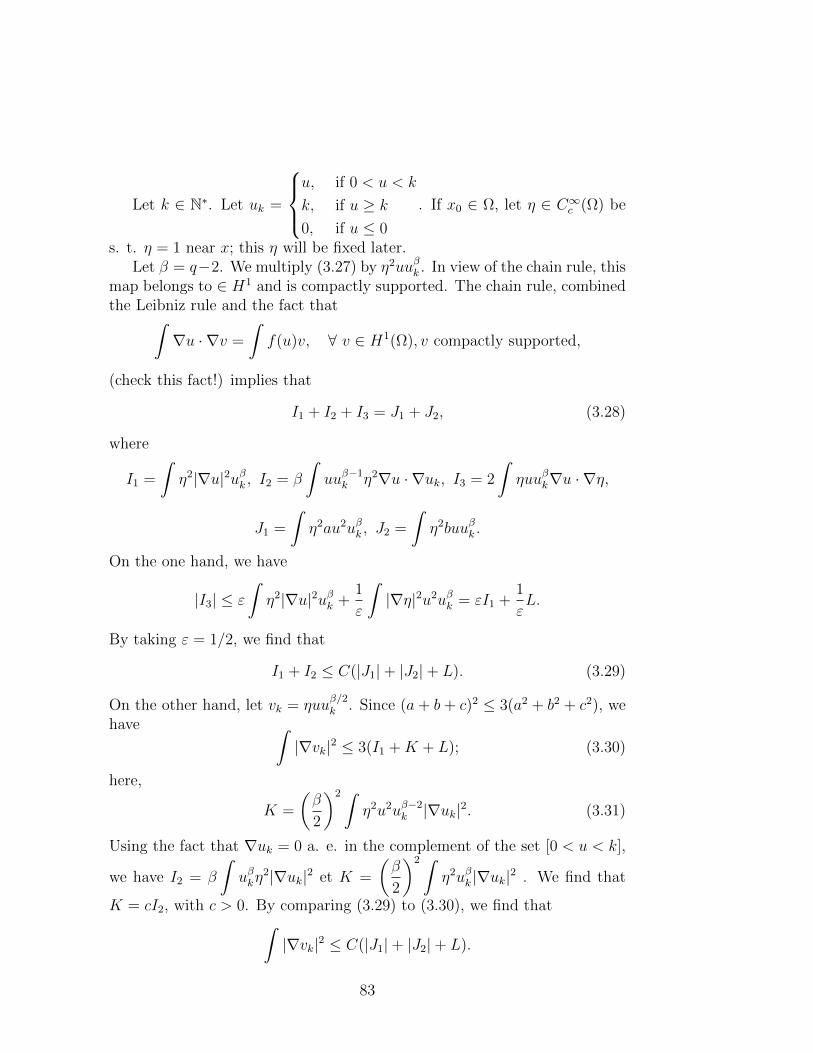
Let k ∈ N∗. Let uk =
u, if 0 < u < k
k, if u ≥ k
0, if u ≤ 0
. If x0 ∈ Ω, let η ∈ C∞c (Ω) be
s. t. η = 1 near x; this η will be fixed later.Let β = q−2. We multiply (3.27) by η2uuβk . In view of the chain rule, this
map belongs to ∈ H1 and is compactly supported. The chain rule, combinedthe Leibniz rule and the fact thatˆ
∇u · ∇v =
ˆf(u)v, ∀ v ∈ H1(Ω), v compactly supported,
(check this fact!) implies that
I1 + I2 + I3 = J1 + J2, (3.28)
where
I1 =
ˆη2|∇u|2uβk , I2 = β
ˆuuβ−1
k η2∇u · ∇uk, I3 = 2
ˆηuuβk∇u · ∇η,
J1 =
ˆη2au2uβk , J2 =
ˆη2buuβk .
On the one hand, we have
|I3| ≤ ε
ˆη2|∇u|2uβk +
1
ε
ˆ|∇η|2u2uβk = εI1 +
1
εL.
By taking ε = 1/2, we find that
I1 + I2 ≤ C(|J1|+ |J2|+ L). (3.29)
On the other hand, let vk = ηuuβ/2k . Since (a+ b+ c)2 ≤ 3(a2 + b2 + c2), we
have ˆ|∇vk|2 ≤ 3(I1 +K + L); (3.30)
here,
K =
(β
2
)2 ˆη2u2uβ−2
k |∇uk|2. (3.31)
Using the fact that ∇uk = 0 a. e. in the complement of the set [0 < u < k],
we have I2 = β
ˆuβkη
2|∇uk|2 et K =
(β
2
)2 ˆη2uβk |∇uk|
2 . We find that
K = cI2, with c > 0. By comparing (3.29) to (3.30), we find thatˆ|∇vk|2 ≤ C(|J1|+ |J2|+ L).
83

The Sobolev embedding implies that
‖vk‖2L2N/(N−2) ≤ C(|J1|+ |J2|+ L). (3.32)
It remains to estimate the integrals in (3.32). Holder’s inequality yields
|J1| ≤ˆ|a|v2
k ≤ ‖a‖LN/2(supp η)‖vk‖2L2N/(N−2) .
Now comes the key point: we choose η. If the support of η is sufficientlysmall, then we have C|J1| ≤ 1/2‖vk‖2
L2N/(N−2) .On the other hand, we have |uk| ≤ |u|, so that
|J2| ≤ C‖u‖q−1Lq−1(supp η) and L ≤ C‖u‖qLq(supp η).
For appropriate η, we find thus
‖vk‖2L2N/(N−2) ≤ C(‖u‖q−1
Lq−1(supp η) + ‖u‖qLq(supp η)).
If we let k → ∞, then we find that η(u+)q/2 ∈ L2N/(N−2) (i. e., that u+ ∈LNq/(N−2) near x) provided that u ∈ Lqloc.
3.27 Proposition. If N ≥ 3 and f is critical, then H1loc solutions of (3.23)
are C∞.
Proof. Write f(t) = g(t)t + b, where b = f(0) ∈ L∞ and g(t) =f(t)− f(0)
tsatisfies |g(t)| ≤ C(1 + |t|4/(N−2)). Then (3.23) rewrites as −∆u = a(x)u+ b,
with a(x) = f(u(x)). Since u ∈ L2N/(N−2)loc , we find that a ∈ LN/2loc . By the
previous lemma, we have u ∈ Lqloc for each q <∞, so that f(u) ∈ Lqloc for eachq <∞. As in the proof of Proposition 3.25, this implies that u ∈ C∞.
3.3.3 Standard estimates
This is a ubiquitous type of results. We will prove here just one. In thesequel, they will be all left to the reader.
3.28 Proposition. Let K, L be two compact subsets of Ω s. t. K ⊂L. If
−∆u = f inL and 1 < p <∞, then
‖u‖W 2,p(K) ≤ C(‖f‖Lp(L) + ‖u‖L1(L)).
84

Before going into the details of the proof, let us explain the philosophyof such estimates (the same applies to all standard estimates involving theLaplace equation): a) the estimate has to be true for the special solutionu = E ∗ f of −∆u = f ; b) the r. h. s. has to contain not only f , but also acontrol of u (think of u = 1, f = 0!).
Proof. Let ζ ∈ C∞c (L) be s. t. ζ = 1 near K. Set g = ζf and let v = E ∗ g.
Then ‖v‖W 2,p(L) ≤ C‖g‖Lp ≤ C‖f‖Lp(L). Let now w = u − v, which isharmonic in a neighborhood M of K. Let 0 < r <dist(K,RN \ M). If
x ∈ K, then
ˆ r
r/2
ˆS(x,s)
|u| ds ≤ C‖w‖L1(L), and thus we may find some
s = s(x) ∈ (r/2, r) s. t.
ˆS(x,s)
|w| ≤ C‖w‖L1(L). In B(x, s), we may
compute w via the Poisson fromula. If we differentiate under the integralsign in the Poisson formula, we find that |∂αw| ≤ C‖w‖L1(L) in B(x, r/4),with C independent of x. Finally, we have ‖w‖W 2,p(B(x,r/4)) ≤ C‖w‖L1(L), sothat ‖w‖W 2,p(K) ≤ C‖w‖L1(L).
We find that
‖u‖W 2,p(K) ≤ ‖v‖W 2,p(K) + ‖w‖W 2,p(K) ≤ C(‖f‖Lp(L) + ‖v‖L1(L) + ‖u‖L1(L)).
We complete the proof by noting that ‖v‖L1(L) ≤ C‖v‖Lp(L) ≤ C‖v‖W 2,p(L) ≤C‖f‖Lp(L).
3.4 Exercises
3.29 Exercise (Hilbert transform). For a compactly supported distribution
f in R, we define its Hilbert transform through the formula Tu =v. p.1
x∗u.
Prove that T is continuous from Lpc into Lp, 1 < p <∞
3.30 Exercise (Regularity for ∂). Let, in R2, ∂ :=1
2∂1 +
1
2ı∂2. Prove that,
for 1 < p <∞, ∂ u ∈ Lploc =⇒ u ∈ W 1,ploc .
3.31 Exercise (Riesz transforms). This exercise relies on the Fourier trans-form of temperate distributions, see, e. g., Hormander.
We define the Riesz transforms through the formulaeRju = F−1
(ξj|ξj|
u
),
j = 1, . . . , N . Here, u ∈ L2(RN). Alternatively, we have Rju = Kj ∗u, where
Kj = F−1
(ξj|ξj|
).
85

a) Let u ∈ L1(RN) be radial. Prove that its Fourier transform is radial, too
b) The same holds if u ∈ L2
c) Let N/2 < α < N . Let uα(x) =1
|x|α. Prove that F (uα) = CαuN−α
Hint: prove first that F (uα) is a radial function. Prove next that F (uα)is homogeneous of degree α−N
d) Prove that Cα =πN/22N−αΓ((N − α)/2)
Γ(α/2)
e) For N ≥ 2, determine the Fourier transform of ∂juN−1. Obtain thatKj ∈ C∞(RN \ 0) satisfies the assumptions of the Calderon-Zygmundtheorem (general form)
f) Derive the following: the Riesz transforms map continuously Lp ∩ L2
(endowed with the Lp norm) into Lp, for 1 < p <∞
g) What becomes the Riesz transform when N = 1?
3.32 Exercise. We prove here that, in the limiting cases uncovered by theCalderon-Zygmund or Korn theorems, there is no good regularity result. Wealso prove that, in general, one cannot replace local regularity conclusionsby global ones (basically, this is due to the fact that u may behave badly atinfinity).
a) Let K,L b RN . Assume that the linear continuous operator S : Lpc →Msends LpK into Lploc (i. e., we have f ∈ LpK =⇒ ΦSf ∈ Lp, for eachΦ ∈ C∞c (RN)). Prove that ΦS is continuous from LpK into LpL, providedsupp Φ ⊂ L
b) By starting with f = ρε, prove that f ∈ L1c 6=⇒ u ∈ W 2,1
loc
c) (Weierstrass’ example) Let v(x) = (x21−x2
2) ln |x|. Prove that −∆v = f ∈C(RN), but that −∆u = f has no C2
loc solution
d) Adapt the following example and find an example of Lipschitz function fs. t. −∆u = f has no solution in C2,1
loc
e) Prove that, if f ∈ L∞c , then the equation −∆u = f need not have asolution in W 2,∞
loc
f) Prove that, if u is harmonic in RN and if |u(x)| ≤ C(1 + |x|)m, then u isa polynomial of degree at most m
86

g) Prove that, if N = 2, then there is some f ∈ Cαc s. t. the equation
−∆u = f has no solution in C2,α
Hint: find first f ∈ Cαc s. t. u 6∈ C2,α, then use the previous question
h) If N ≥ 3, prove that f ∈ Cαc =⇒ u ∈ C2,α.
i) Let 1 < p < ∞ and let N = 2. Prove that, if f ∈ Lpc , then we need nothave u ∈ W 2,p
j) If N ≥ 3 and p ≤ N/(N − 2), prove that f ∈ Lpc 6=⇒ u ∈ W 2,p
k) If N ≥ 3 and p > N/(N − 2), prove that f ∈ Lpc =⇒ u ∈ W 2,p.
3.33 Exercise. We try to discuss here to what extent the would be impli-cations (*) f ∈ L1
c =⇒ ∂j∂ku ∈ L1loc and (**) f ∈ L∞c =⇒ ∂j∂ku ∈ L∞loc are
wrong. If (*) where true, then we would have, via the Sobolev embeddings,
∇u ∈ LN/(N−1)loc and, if N = 2, u ∈ L∞loc. Similarly, (**), if true, would imply
∇u ∈ Liploc.In this exercise, we give a qualitative form to the fact that the last im-
plications are almost true. This is expressed in the context of the BMO(=bounded mean oscillations) space of John et Nirenberg, defined as follows:
f ∈ BMO⇐⇒ ∃K = K(f) s. t.
C
∣∣∣∣f − C
f
∣∣∣∣ ≤ K, for each cube C ⊂ RN .
For a thorough study of BMO, we refer to Stein, Chapter IV. We mentionhere, without proof, the John-Nirenberg inequality: there is some c = c(N)s. t. exp(cf/K) ∈ L1
loc. In particular, f ∈ BMO=⇒ f ∈ Lploc for p <∞.
a) If m ∈ R, prove that
C
∣∣∣∣f − C
f
∣∣∣∣ ≤ 2
C
|f−m|. Consequently, in order
to prove that f ∈ BMO, it suffices to prove that, for each cube C, there
is some m s. t.
C
|f −m| ≤ K
b) Prove that x 7→ ln |x| ∈ BMO
c) If f ∈ L∞c , prove that ∂j∂ku ∈ BMO
d) If f ∈ L∞c , prove that |∇u(x)−∇u(y)| ≤ C|x− y|(1 + | ln |x− y||)
e) If f ∈ L1c , prove that ∇u ∈ W 1,q
loc for q < N/(N − 1). The same holds if fis a compactly supported measure
f) If f ∈ L1c and N = 2, prove that u ∈ BMO. The same holds if f is a
compactly supported measure.
87

3.34 Exercise. We discuss here various consequences of the maximal func-tion theorem. Recall that, if u ∈ L1
loc(RN), then the maximal function of u at
x is defined as Mu(x) = supx∈C
C
|u(y)| dy. Here, the supremum is taken over
the cubes (or balls) containing x. The maximal function is a Borel function.Recall the following special case of the Hardy-Littlewood maximal theorem:
if u ∈ L1, then there is some K = K(N) s. t. |Mu(x) > t| ≤ K‖u‖L1
t,
∀ t > 0. For a proof, see the first pages in Stein.
a) Let ϕ be integrable, radial, non increasing. Prove that |u ∗ ϕε(x)| ≤‖ϕ‖L1Mu(x), ∀ x, ∀ ε > 0Hint: start with a step function
b) If ρ is a mollifier, prove that there is some C = C(ρ) s. t. |u ∗ ρε(x)| ≤CMu(x), ∀ x, ∀ ε > 0
c) If u ∈ L1loc, prove that u ∗ ρε → u a. e. as ε→ 0
Hint: start with the case where u ∈ C∞c (RN). For the general case, usethe converse to the dominated convergence theorem
d) (Lebesgue’s differentiation theorem) If u ∈ L1loc(RN), prove that
limx∈C, |C|→0
C
|u(y)− u(x)| dy = 0 for a. e. x.
In particular, we have limx∈C, |C|→0
C
u(y) dy = u(x) for a. e. x.
88