Introduzione a MATLAB Paolo Valigi

Dipartimento di Ingegneria Università degli Studi di Perugia

2 MATLAB - Basic

Credits

Based on material from the net, and in particular:

•  Sergio Bittanti, Politecnico di Milano (Technical University of Milan)

•  Ashok Krishnamurthy, Ohio Supercomputer Center

3 MATLAB - Basic

Table of Contents

•  Overview •  Basic Interfaces •  Arrays, Matrices, Operators •  Programming •  Data I/O

•  Basic Data Analysis •  Numerical Analysis •  Graphics, Data Visualization, Movies •  Inter-language Programming

Overview

5

MATLAB

•  “MATrix LABoratory” •  Powerful, extensible, highly integrated

computation, programming, visualization, and simulation package

•  Widely used in engineering, mathematics, and

science •  Why?

6 MATLAB - Basic

MATLAB’s Appeal

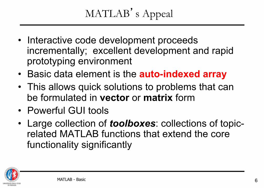
•  Interactive code development proceeds incrementally; excellent development and rapid prototyping environment

•  Basic data element is the auto-indexed array •  This allows quick solutions to problems that can

be formulated in vector or matrix form •  Powerful GUI tools •  Large collection of toolboxes: collections of topic-

related MATLAB functions that extend the core functionality significantly

7 MATLAB - Basic

Toolboxes, Software, & Links

8 MATLAB - Basic

MATLAB System

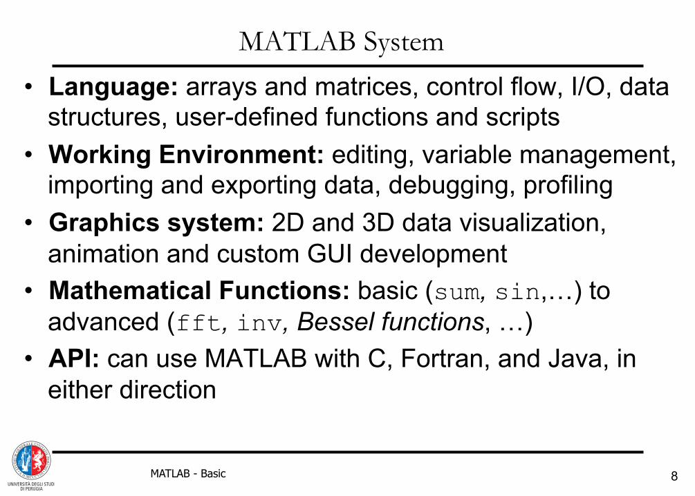
•  Language: arrays and matrices, control flow, I/O, data structures, user-defined functions and scripts

•  Working Environment: editing, variable management, importing and exporting data, debugging, profiling

•  Graphics system: 2D and 3D data visualization, animation and custom GUI development

•  Mathematical Functions: basic (sum, sin,…) to advanced (fft, inv, Bessel functions, …)

•  API: can use MATLAB with C, Fortran, and Java, in either direction

9 MATLAB - Basic

Online MATLAB Resources

•  www.mathworks.com/!•  http://it.mathworks.com/academia/student_center/tutorials/launchpad.html!

•  https://www.youtube.com/watch?v=QOJCvHUkJSs!

•  http://www.uniroma2.it/didattica/CMCA3/deposito/MATLAB_base.pdf!

•  …. mille altre fonti e pagine

Basic Interfaces

11 MATLAB - Basic

Main MATLAB Interface

12 MATLAB - Basic

Some MATLAB Development Windows

•  Command Window: where you enter commands •  Command History: running history of commands which is

preserved across MATLAB sessions •  Current directory: Default is $matlabroot/work •  Workspace: GUI for viewing, loading and saving MATLAB

variables •  Array Editor: GUI for viewing and/or modifying contents of

MATLAB variables (openvar varname or double-click the array’s name in the Workspace)

•  Editor/Debugger: text editor, debugger; editor works with file types in addition to .m (MATLAB “m-files”)

13 MATLAB - Basic

MATLAB Editor Window

14 MATLAB - Basic

MATLAB Help Window (Very Powerful)

15 MATLAB - Basic

Command-Line Help �: List of MATLAB Topics

>> help HELP topics: matlab\general - General purpose commands. matlab\ops - Operators and special characters. matlab\lang - Programming language constructs. matlab\elmat - Elementary matrices and matrix manipulation. matlab\elfun - Elementary math functions. matlab\specfun - Specialized math functions. matlab\matfun - Matrix functions - numerical linear algebra. matlab\datafun - Data analysis and Fourier transforms. matlab\polyfun - Interpolation and polynomials. matlab\funfun - Function functions and ODE solvers. matlab\sparfun - Sparse matrices. matlab\scribe - Annotation and Plot Editing. matlab\graph2d - Two dimensional graphs. matlab\graph3d - Three dimensional graphs. matlab\specgraph - Specialized graphs. matlab\graphics - Handle Graphics. …etc...

16 MATLAB - Basic

Command-Line Help �: List of Topic Functions

>> help matfun Matrix functions - numerical linear algebra. Matrix analysis. norm - Matrix or vector norm. normest - Estimate the matrix 2-norm. rank - Matrix rank. det - Determinant. trace - Sum of diagonal elements. null - Null space. orth - Orthogonalization. rref - Reduced row echelon form. subspace - Angle between two subspaces.

…

17 MATLAB - Basic

Command-Line Help �: Function Help >> help det DET Determinant. DET(X) is the determinant of the square matrix X. Use COND instead of DET to test for matrix singularity. See also cond. Overloaded functions or methods (ones with the same name in other directories)

help laurmat/det.m Reference page in Help browser doc det

18 MATLAB - Basic

Keyword Search of Help Entries

>> lookfor who newton.m: % inputs: 'x' is the number whose square

root we seek testNewton.m: % inputs: 'x' is the number whose

square root we seek WHO List current variables. WHOS List current variables, long form. TIMESTWO S-function whose output is two times its

input. >> whos Name Size Bytes Class Attributes ans 1x1 8 double fid 1x1 8 double i 1x1 8 double

Variables (Arrays) and Operators

20 MATLAB - Basic

Variable Basics

no declarations needed

mixed data types

semi-colon suppresses output of the calculation’s result

>> 16 + 24 ans = 40 >> product = 16 * 23.24 product = 371.84 >> product = 16 *555.24; >> product product = 8883.8

21 MATLAB - Basic

Variable Basics

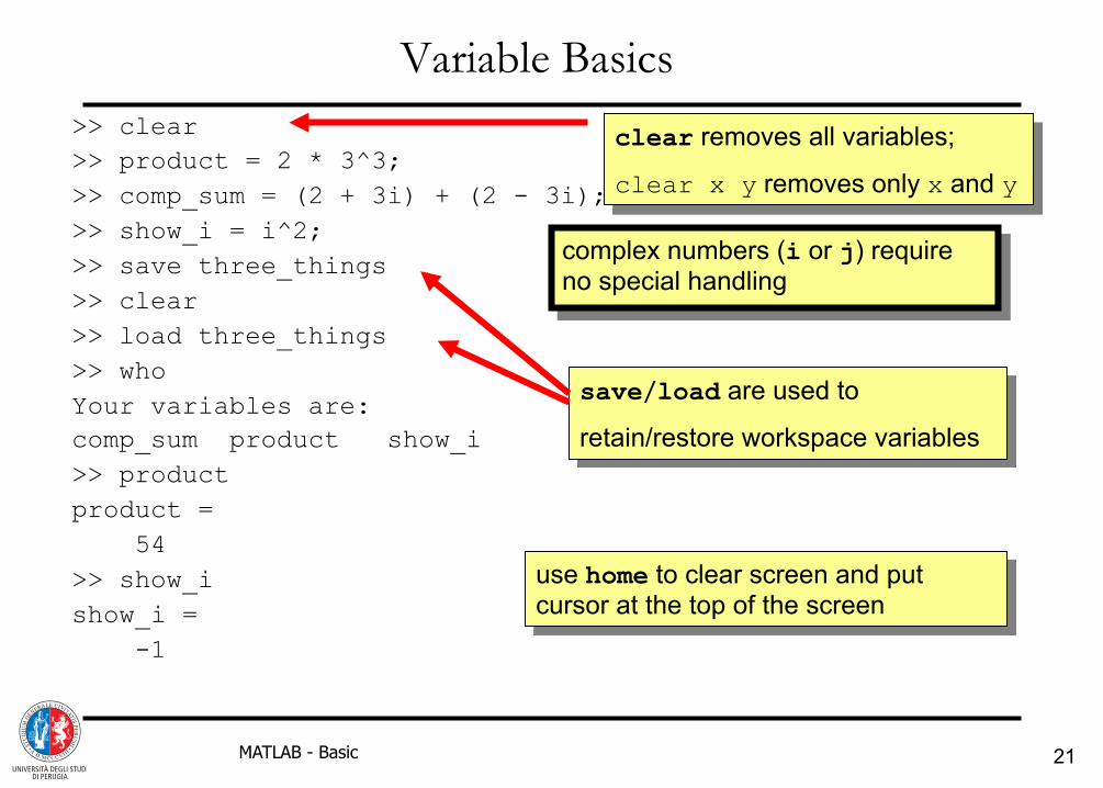
complex numbers (i or j) require no special handling

clear removes all variables;

clear x y removes only x and y

save/load are used to

retain/restore workspace variables

>> clear >> product = 2 * 3^3; >> comp_sum = (2 + 3i) + (2 - 3i); >> show_i = i^2; >> save three_things >> clear >> load three_things >> who Your variables are: comp_sum product show_i >> product product = 54 >> show_i show_i = -1

use home to clear screen and put cursor at the top of the screen

22 MATLAB - Basic

MATLAB Data • 

The basic data type used in MATLAB is the double precision array •  No declarations needed: MATLAB automatically allocates required memory •  Resize arrays dynamically •  To reuse a variable name, simply use it in the left hand side of an assignment statement •  MATLAB displays results in scientific notation

o  Use File/Preferences and/or format function to change default §  short (5 digits), long (16 digits) §  format short; format compact

23 MATLAB - Basic

Variables Revisited •  Variable names are case sensitive and over-written when re-used •  Basic variable class: Auto-Indexed Array

–  Allows use of entire arrays (scalar, 1-D, 2-D, etc…) as operands

–  Vectorization: Always use array operands to get best performance (see next slide)

•  Terminology: “scalar” (1 x 1 array), “vector” (1 x N array), “matrix” (M x N array)

•  Special variables/functions: ans, pi, eps, inf, NaN, i, nargin, nargout, ...

•  Commands who (terse output) and whos (verbose output) show

variables in Workspace

24 MATLAB - Basic

Vectorization Example*

>> type slow.m tic; x=0.1; for k=1:199901 y(k)=besselj(3,x) + log(x);

x=x+0.001; end toc; >> slow Elapsed time is 21.861525 seconds. *times measured on this MacBook

>> type fast.m tic; x=0.1:0.001:200; y=besselj(3,x) + log(x); toc; >> fast Elapsed time is 0.216881 seconds. Roughly 100 times faster without use of for loop

25 MATLAB - Basic

Operating on Scalars

>> z = 3 + i*5; >> z = 3 + j*5;

Matlab operates also on complex numbers

i and j are pre-defined constants Unless overwritten !!

>> r = real(z) >> w = imag(z)

Real part and imaginary of complex z!

>> m = abs(z) >> p = phase(z)

Complex modulus (magnitude) and phase (radians) of complex z!

26 MATLAB - Basic

Matrices: Magic Squares

This matrix is called a “magic square”

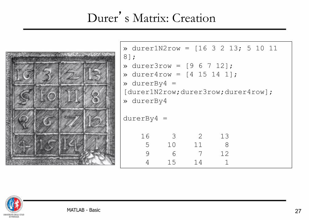
Interestingly, Durer also dated this engraving by placing 15 and 14 side-by-side in the magic square.

http://en.wikipedia.org/wiki/Magic_square!

Sagrada Família Barcelona Antoni Gaudí Josep Maria Subirachs

27 MATLAB - Basic

Durer’s Matrix: Creation

» durer1N2row = [16 3 2 13; 5 10 11 8]; » durer3row = [9 6 7 12]; » durer4row = [4 15 14 1]; » durerBy4 = [durer1N2row;durer3row;durer4row]; » durerBy4 durerBy4 = 16 3 2 13 5 10 11 8 9 6 7 12 4 15 14 1

28 MATLAB - Basic

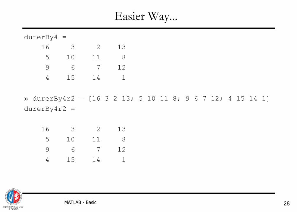
Easier Way...

durerBy4 = 16 3 2 13

5 10 11 8

9 6 7 12

4 15 14 1

» durerBy4r2 = [16 3 2 13; 5 10 11 8; 9 6 7 12; 4 15 14 1]

durerBy4r2 =

16 3 2 13

5 10 11 8

9 6 7 12

4 15 14 1

29 MATLAB - Basic

Working with matrices

>> matrix=[1 2 3; 3 4 5; 0 0 1]

matrix =

1 2 3

3 4 5

0 0 1

>> det(matrix)

ans =

-2

30 MATLAB - Basic

Working with matrices (2)

>> rank(matrix) ans =

3

>> size(matrix)

ans =

3 3

>> matinv=inv(matrix)

matinv =

-2.0000 1.0000 1.0000

1.5000 -0.5000 -2.0000

0 0 1.0000

31 MATLAB - Basic

Working with matrices (3)

>> p=poly(matrix) p =

1.0000 -6.0000 3.0000 2.0000

>> eigmat=eig(matrix)

eigmat =

-0.3723

5.3723

1.0000

>> roots(p)

ans =

5.3723

1.0000

-0.3723

32 MATLAB - Basic

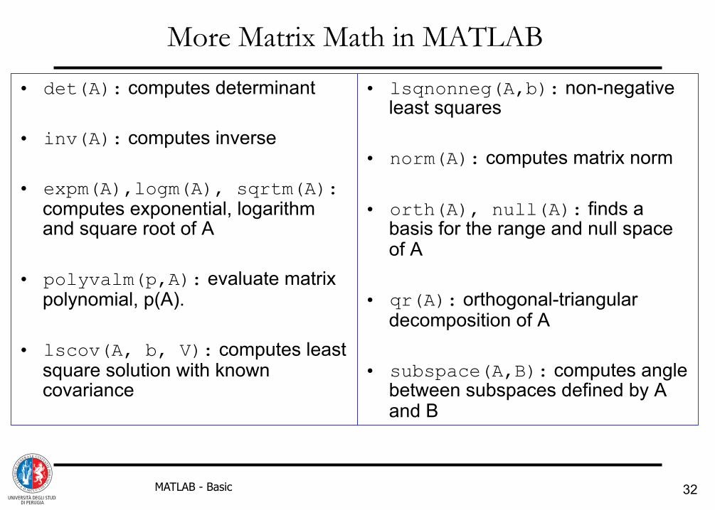
More Matrix Math in MATLAB

•  det(A): computes determinant •  inv(A): computes inverse •  expm(A),logm(A), sqrtm(A):

computes exponential, logarithm and square root of A

•  polyvalm(p,A): evaluate matrix

polynomial, p(A). •  lscov(A, b, V): computes least

square solution with known covariance

•  lsqnonneg(A,b): non-negative least squares

•  norm(A): computes matrix norm •  orth(A), null(A): finds a

basis for the range and null space of A

•  qr(A): orthogonal-triangular

decomposition of A •  subspace(A,B): computes angle

between subspaces defined by A and B

33 MATLAB - Basic

Working with polinomials

>> p1=[1 1] p1 =

1 1

>> p2=[1 2]

p2 =

1 2

>> p12=conv(p1,p2)

p12 =

1 3 2

>> roots(p12)

ans =

-2

-1

>> polyval(p12,-1) ans =

0

>> polyval(p12,1)

ans =

6

>> p13=poly([-1, -3])

p13 =

1 4 3

>> polyder(p13)

ans =

2 4

34 MATLAB - Basic

Multidimensional Arrays >> r = randn(2,3,4) % create a 3 dimensional array filled with normally distributed random numbers r(:,:,1) =

-0.6918 1.2540 -1.4410

0.8580 -1.5937 0.5711

r(:,:,2) =

-0.3999 0.8156 1.2902

0.6900 0.7119 0.6686

r(:,:,3) =

1.1908 -0.0198 -1.6041

-1.2025 -0.1567 0.2573

r(:,:,4) =

-1.0565 -0.8051 0.2193

1.4151 0.5287 -0.9219

randn(2,3,4): 3 dimensions, filled with normally distributed random numbers

“%” sign precedes comments, MATLAB ignores the rest of the line

35 MATLAB - Basic

Character Strings >> hi = ' hello'; >> class = 'MATLAB'; >> hi hi = hello >> class class = MATLAB >> greetings = [hi class] greetings = helloMATLAB >> vgreetings = [hi;class] vgreetings = hello MATLAB

semi-colon: join vertically

concatenation with blank or with “,”

36 MATLAB - Basic

Character Strings as Arrays >> greetings

greetings =

helloMATLAB

>> vgreetings = [hi;class]

vgreetings =

hello

MATLAB

>> hi = 'hello'

hi =

hello

>> vgreetings = [hi;class]

??? Error using ==> vertcat

CAT arguments dimensions are not consistent.

note deleted space at beginning of word; results in error

37 MATLAB - Basic

yo =

Hello

Class

>> ischar(yo)

ans =

1

>> strcmp(yo,yo)

ans =

1

String Functions

returns 1 if argument is a character array and 0 otherwise

returns 1 if string arguments are the same and 0 otherwise; strcmpi ignores case

38 MATLAB - Basic

Set Functions Arrays are ordered sets: >> a = [1 2 3 4 5] a = 1 2 3 4 5 >> b = [3 4 5 6 7] b = 3 4 5 6 7 >> isequal(a,b) ans = 0 >> ismember(a,b) ans = 0 0 1 1 1

returns true (1) if arrays are the same size and have the same values

returns 1 where a is in b and 0 otherwise

39 MATLAB - Basic

>> durer = [16 3 2 13; 5 10 11 8; 9 6 7 12; 4 15 14 1] durer = 16 3 2 13 5 10 11 8 9 6 7 12 4 15 14 1 >> % durer's matrix is "magic" in that all rows, columns, >> % and main diagonals sum to the same number >> column_sum = sum(durer) % MATLAB operates column-wise column_sum = 34 34 34 34

Matrix Operations

MATLAB also has magic(N) (N > 2) function

40 MATLAB - Basic

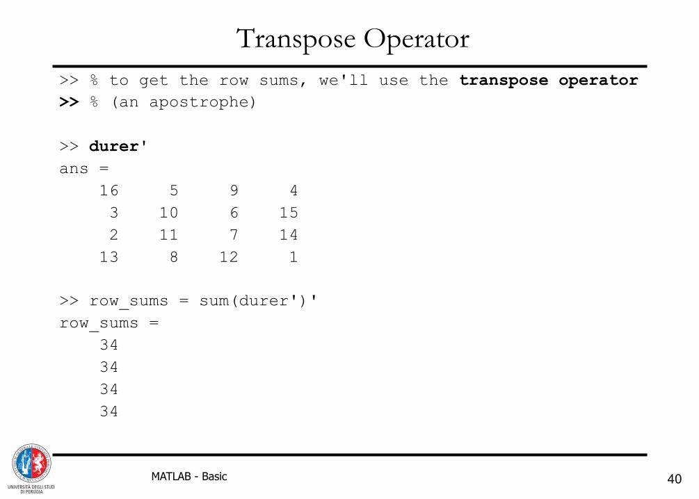
Transpose Operator >> % to get the row sums, we'll use the transpose operator >> % (an apostrophe) >> durer' ans = 16 5 9 4 3 10 6 15 2 11 7 14 13 8 12 1 >> row_sums = sum(durer')' row_sums = 34 34 34 34

41 MATLAB - Basic

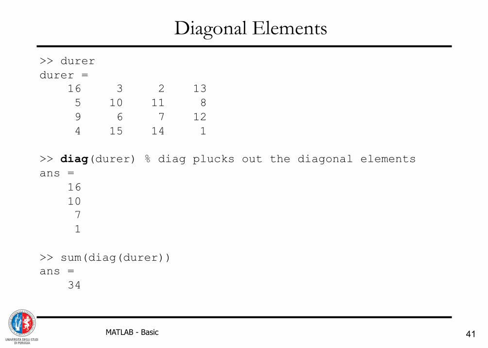
Diagonal Elements >> durer durer = 16 3 2 13 5 10 11 8 9 6 7 12 4 15 14 1 >> diag(durer) % diag plucks out the diagonal elements ans = 16 10 7 1 >> sum(diag(durer)) ans = 34

42 MATLAB - Basic

The Other Diagonal… >> durer durer = 16 3 2 13 5 10 11 8 9 6 7 12 4 15 14 1 >> fliplr(durer) % “flip left-right” ans = 13 2 3 16 8 11 10 5 12 7 6 9 1 14 15 4 >> sum(diag(fliplr(durer))) ans = 34

43 MATLAB - Basic

Matrix Subscripting >> durer durer = 16 3 2 13 5 10 11 8 9 6 7 12 4 15 14 1 >> diag_sum = durer(1,1) + durer(2,2) + durer(3,3) diag_sum = 33 >> durer(4,4) = pi durer = 16.0000 3.0000 2.0000 13.0000 5.0000 10.0000 11.0000 8.0000 9.0000 6.0000 7.0000 12.0000 4.0000 15.0000 14.0000 3.1416 >> durer(4,4) = 1

44 MATLAB - Basic

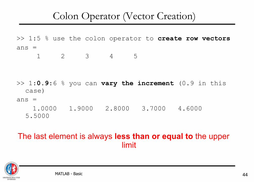
Colon Operator (Vector Creation) >> 1:5 % use the colon operator to create row vectors ans = 1 2 3 4 5 >> 1:0.9:6 % you can vary the increment (0.9 in this

case) ans = 1.0000 1.9000 2.8000 3.7000 4.6000

5.5000

The last element is always less than or equal to the upper

limit

45 MATLAB - Basic

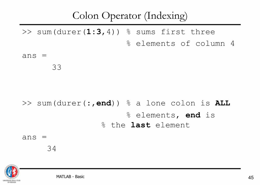
Colon Operator (Indexing) >> sum(durer(1:3,4)) % sums first three % elements of column 4

ans =

33

>> sum(durer(:,end)) % a lone colon is ALL % elements, end is % the last element

ans = 34

46 MATLAB - Basic

The “Dot Operator” •  By default and whenever possible MATLAB will

perform true matrix operations (+ - *). The operands in every arithmetic expression are considered to be matrices.

•  If, on the other hand, the user wants the scalar version of an operation a “dot” must be put in front of the operator, e.g., .*. Matrices can still be the operands but the mathematical calculations will be performed element-by-element.

•  A comparison of matrix multiplication and scalar multiplication is shown on the next slide.

47 MATLAB - Basic

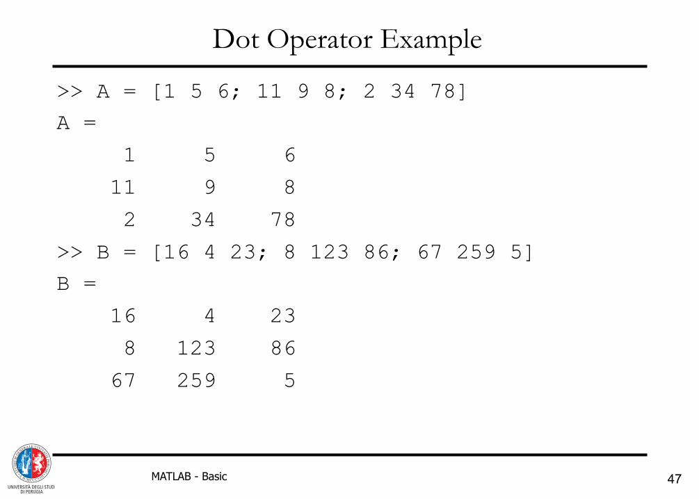
Dot Operator Example

>> A = [1 5 6; 11 9 8; 2 34 78] A =

1 5 6

11 9 8

2 34 78

>> B = [16 4 23; 8 123 86; 67 259 5] B =

16 4 23

8 123 86

67 259 5

48 MATLAB - Basic

Dot Operator Example (cont.) >> C = A * B % “normal” matrix multiply C =

458 2173 483

784 3223 1067

5530 24392 3360

>> CDOT = A .* B % element-by-element CDOT =

16 20 138

88 1107 688 134 8806 390

49 MATLAB - Basic

Easy 2-D Graphics

>> x = [0: pi/100: pi]; % [start: increment: end] >> y = sin(x);

>> plot(x,y), title('Simple Plot')

50 MATLAB - Basic

Adding Another Curve

Line color, style, marker type, all within single quotes; type

>> doc LineSpec

for all available line properties

>> z = cos(x); >> plot(x,y,'g.',x,z,'b-.'),title('More complicated')

51 MATLAB - Basic

Changing scales

>> help loglog loglog Log-log scale plot. loglog(...) is the same as PLOT(...), except logarithmic scales are used for both the X- and Y- axes.

>> help semilogx

semilogx Semi-log scale plot. semilogx(...) is the same as PLOT(...), except a

logarithmic (base 10) scale is used for the X-axis.

>> help semilogy

semilogy Semi-log scale plot. semilogy(...) is the same as PLOT(...), except a

logarithmic (base 10) scale is used for the Y-axis.

Programming

53 MATLAB - Basic

•  MATLAB m-file Editor –  To start: click icon or enter edit command in

Command Window, e.g., >> edit test.m •  Scripts and Functions •  Decision Making/Looping

–  if/else –  switch –  for and while

•  Running Operating System Commands

Outline

54 MATLAB - Basic

You can save and run the file/function/script in one step by clicking here

Tip: semi-colons suppress printing, commas (and semi-colons) allow multiple commands on one line, and 3 dots (…) allow continuation of lines without execution

m-file Editor Window

55 MATLAB - Basic

Scripts and Functions

•  Scripts do not accept input arguments, nor do they produce output arguments. Scripts are simply MATLAB commands written into a file. They operate on the existing workspace.

•  Functions accept input arguments and produce output variables. All internal variables are local to the function and commands operate on the function workspace.

•  A file containing a script or function is called an m-file •  If duplicate functions (names) exist, the first in the

search path (from path command) is executed.

56 MATLAB - Basic

function [a b c] = myfun(x, y) b = x * y; a = 100; c = x.^2; >> myfun(2,3) % called with zero outputs ans = 100 >> u = myfun(2,3) % called with one output u = 100 >> [u v w] = myfun(2,3) % called with all outputs u = 100 v = 6 w = 4

Functions – First Example Write these two lines to a file myfun.m and save it on MATLAB’s path

Any return value which is not stored in an output variable is simply discarded

57 MATLAB - Basic

Function Syntax Summary •  If the m-file name and function name differ, the file

name takes precedence •  Function names must begin with a letter •  First line must contain function followed by the most

general calling syntax •  Statements after initial contiguous comments (help lines)

are the body of the function •  Terminates on the last line or a return statement

58 MATLAB - Basic

Function Syntax Summary (cont.)

•  error and warning can be used to test and continue execution (error-handling)

•  Scripts called in m-file functions are evaluated in the

function workspace •  Additional functions (subfunctions) can be included in an

m-file •  Use which command to determine precedence, e.g., >> which title C:\MATLAB71\toolbox\matlab\graph2d\title

59 MATLAB - Basic

if/elseif/else Statement >> A = 2; B = 3; >> if A > B 'A is bigger' elseif A < B 'B is bigger' elseif A == B 'A equals B' else error('Something odd is happening') end ans = B is bigger

60 MATLAB - Basic

switch Statement

>> n = 8 n = 8 >> switch(rem(n,3)) case 0 m = 'no remainder' case 1 m = ‘the remainder is one' case 2 m = ‘the remainder is two' otherwise error('not possible') end m = the remainder is two

61 MATLAB - Basic

for Loop >> for i = 2:5

for j = 3:6

a(i,j) = (i + j)^2

end

end

>> a

a =

0 0 0 0 0 0

0 0 25 36 49 64

0 0 36 49 64 81

0 0 49 64 81 100

0 0 64 81 100 121

62 MATLAB - Basic

while Loop

>> b = 4; a = 2.1; count = 0; >> while b - a > 0.01 a = a + 0.001; count = count + 1; end >> count count = 1891

63 MATLAB - Basic

MATLAB’s Search Path

•  Is name a variable?

•  Is name a built-in function?

•  Does name exist in the current directory?

•  Does name exist anywhere in the search path?

•  “Discovery functions”: who, whos, what, which, exist, help, doc, lookfor, dir, ls, ...

64 MATLAB - Basic

Changing the Search Path

•  The addpath command adds directories to the MATLAB search path. The specified directories are added to the beginning of the search path.

•  rmpath is used to remove paths from the search path

>> path

MATLABPATH

E:\MATLAB\R2006b\work E:\MATLAB\R2006b\work\f_funcs E:\MATLAB\R2006b\work\na_funcs E:\MATLAB\R2006b\work\na_scripts E:\MATLAB\R2006b\toolbox\matlab\general E:\MATLAB\R2006b\toolbox\matlab\ops

>> addpath('c:\'); >> matlabpath

MATLABPATH

c:\ E:\MATLAB\R2006b\work E:\MATLAB\R2006b\work\f_funcs E:\MATLAB\R2006b\work\na_funcs E:\MATLAB\R2006b\work\na_scripts E:\MATLAB\R2006b\toolbox\matlab\general E:\MATLAB\R2006b\toolbox\matlab\ops

65 MATLAB - Basic

Common OS Commands

•  ls / dir provide a directory listing of the current directory

•  pwd shows the current directory

>> ls . .. sample.m >>

>> pwd ans = e:\Program Files\MATLAB\R2006b\work >>

66 MATLAB - Basic

Running OS Commands

•  The system command can be used to run OS commands •  On Unix systems, the unix command can be used as well •  On DOS systems, the corresponding command is dos

>> dos('date') The current date is: Thu 01/04/2007 Enter the new date: (mm-dd-yy) ans = 0

Data I/O

68 MATLAB - Basic

Loading and Saving Workspace Variables

•  MATLAB can load and save data in .MAT format

•  .MAT files are binary files that can be transferred across platforms; as much accuracy as possible is preserved.

•  Load: load filename OR A = load(‘filename’)

loads all the variables in the specified file (the default name is MATLAB.MAT)

•  Save: save filename variables saves the specified variables (all variables by default) in the specified file (the default name is MATLAB.MAT)

69 MATLAB - Basic

ASCII File Read/Write

load and save can also read and write ASCII files with rows of space separated values: •  load test.dat –ascii

•  save filename variables (options are ascii, double, tabs, append)

•  save example.dat myvar1 myvar2 -ascii -double

70 MATLAB - Basic

Import Wizard Import ASCII and binary files using the Import Wizard. Type uiimport at the Command line or choose Import Data from the File menu.

71 MATLAB - Basic

Low-Level File I/O Functions •  File Opening and Closing

–  fclose: Close one or more open files –  fopen: Open a file or obtain information about open files

•  Unformatted I/O –  fread: Read binary data from file –  fwrite: Write binary data to a file

•  Formatted I/O –  fgetl: Return the next line of a file as a string

without line terminator(s) –  fgets: Return the next line of a file as a string with line terminator(s) –  fprintf: Write formatted data to file –  fscanf: Read formatted data from file

72 MATLAB - Basic

Format String Specification

%-12.5e initial % character width and

precision

conversion specifier

alignment flag

Specifier Description %c Single character %d Decimal notation (signed) %e Exponential notation %f Fixed-point notation %g The more compact of %e or %f %o Octal notation (unsigned) %s String of characters %u Decimal notation (unsigned) %x Hexadecimal notation ...others...

73 MATLAB - Basic

Other Formatted I/O Commands •  fgetl: line = fgetl(fid);

reads next line from file without line terminator •  fgets: line = fgets(fid);

reads next line from file with line terminator •  textread: [A,B,C,...] = textread('filename','format',N)

reads N lines of formatted text from file filename •  sscanf: A = sscanf(s, format, size);

reads string under format control •  sprintf: s = sprintf(format, A);

writes formatted data to a string

74 MATLAB - Basic

•  Multidimensional MATLAB arrays •  Access elements using textual field designators •  Create structures by using periods (.): >> class.name = ‘MATLAB’;

>> class.day1 = ‘2/27/07’;

>> class.day2 = ‘2/28/07’;

>> class

class =

name: ‘MATLAB’

day1: ‘2/27/07’

day2: ‘2/28/07’

Structures

75 MATLAB - Basic

•  Structures are arrays (no surprise) •  Fields can be added one at a time: >> class(2).name = ‘MPI’;

>> class(2).day1 = ‘TBA’;

>> class(2).day2 = ‘TBA’; •  Can also use a single statement: >> class(2) = struct(‘name’,‘MPI’,... ‘day1’,‘TBA’,‘day2’,‘TBA’)

Manipulating Structures

76 MATLAB - Basic

•  Consider the simple structure >> exam.name = ‘Jim Kirk’;

>> exam.score = 79;

>> exam(2).name = ‘Janice Lester’;

>> exam(2).score = 89; >> [exam.score] ans =

79 89

Manipulating Structures (cont.)

square brackets produce a numeric row vector

Basic Data Analysis

78 MATLAB - Basic

Basic system analysis

•  Basic, and more advanced, systems analysis is easily accomplished in MATLAB.

•  Remember that the MATLAB default is to

assume variables are matrices.

79

To describe a continuous time system, the ss command (state space) is available

     dx/dt  =  Ax(t)  +  Bu(t)                            y(t)  =  Cx(t)  +  Du(t)  >>  system=  ss(A,B,C,D)  [ss(A,B,C,0)];  

                       as well as the tf command (transfer function)

W(s) = num(s)/den(s) >>  system_5=  5(num,den);

Similar commands for discrete time and sampled-data system

Basic system analysis (2)

80

•  Impulse response: –  impulse(system) –  Impulse(system_tf)

•  Step response: –  step(system) –  step(system_tf)

•  Response to a generic input signal: –  [y,t,x] = lsim(system,u,t,x0)

•  Frequency response:

–  Bode(system)

Basic system analysis (3)

81 MATLAB - Basic

Basic Data Analysis

•  Basic, and more advanced, statistical analysis is easily accomplished in MATLAB.

•  Remember that the MATLAB default is to

assume vectors are columnar. •  Each column is a variable, and each row is an

observation.

82 MATLAB - Basic

Vibration Sensors Data

Each column is the raw rpm sensor data from a different sensor used in an instrumented engine test. The rows represent the times readings were made.

83 MATLAB - Basic

Plotting the Data

Note that in this case the plot command generates one time-series for each column of the data matrix

>> plot(rpm_raw) >> xlabel('sample number - during time slice'); >> ylabel('Unfiltered RPM Data'); >> title(‘3 sequences of samples from RPM sensor’)

84 MATLAB - Basic

Average of the Data:

Applying the mean function to the data matrix yields the mean of each column

But you can easily compute the mean of the entire matrix (applying a function to either a single row or a single column results in the function applied to the column, or the row, i.e., in both cases, the application is to the vector).

1

2

>> mean(rpm_raw) ans = 1081.4 1082.8 1002.7 >> mean(mean(rpm_raw)) ans = 1055.6

85 MATLAB - Basic

The mean Function

But we can apply the mean function along any dimension

So we can easily obtain the row means

3

>> help mean MEAN Average or mean value. For vectors, MEAN(X) is the mean value of the elements in X. For matrices, MEAN(X) is a row vector containing the mean value of each column. For N-D arrays, MEAN(X) is the mean value of the elements along the first non-singleton dimension of X. MEAN(X,DIM) takes the mean along the dimension DIM of X. Example: If X = [0 1 2 3 4 5] then mean(X,1) is [1.5 2.5 3.5] and mean(X,2) is [1 4] >> mean(rpm_raw, 2)

ans = 1045.7 1064.7 1060.7 1055 1045

86 MATLAB - Basic

max and its Index

We can compute the max of the entire matrix, or of any dimension

1 2 MAX Largest component. For vectors, MAX(X) is the largest

element in X. For matrices, MAX(X) is a row vector containing the

maximum element from each column. For N-D arrays, MAX(X) operates along

the first non-singleton dimension. [Y,I] = MAX(X) returns the indices of

the maximum values in vector I. If the values along the first non-

singleton dimension contain more than one maximal element, the index

of the first one is returned.

>> max(rpm_raw) ans = 1115 1120 1043 >> max(max(rpm_raw)) ans = 1120 >> [y,i] = max(rpm_raw) y = 1115 1120 1043 i = 8 2 17 max along the columns

87 MATLAB - Basic

Data Analysis: Histogram

HIST Histogram. N = HIST(Y) bins the elements of Y into 10 equally spaced containers and returns the number of elements in each container. If Y is a matrix, HIST works down the columns. N = HIST(Y,M), where M is a scalar, uses M bins. N = HIST(Y,X), where X is a vector, returns the distribution of Y among bins with centers specified by X. The first bin includes data between -inf and the first center and the last bin includes data between the last bin and inf. Note: Use HISTC if it is more natural to specify bin edges instead. . . .

88 MATLAB - Basic

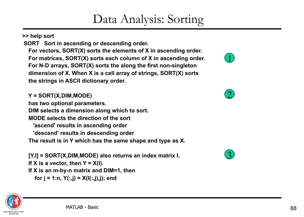
Data Analysis: Sorting

1

2

3

>> help sort SORT Sort in ascending or descending order. For vectors, SORT(X) sorts the elements of X in ascending order. For matrices, SORT(X) sorts each column of X in ascending order. For N-D arrays, SORT(X) sorts the along the first non-singleton dimension of X. When X is a cell array of strings, SORT(X) sorts the strings in ASCII dictionary order. Y = SORT(X,DIM,MODE) has two optional parameters. DIM selects a dimension along which to sort. MODE selects the direction of the sort 'ascend' results in ascending order 'descend' results in descending order The result is in Y which has the same shape and type as X. [Y,I] = SORT(X,DIM,MODE) also returns an index matrix I. If X is a vector, then Y = X(I). If X is an m-by-n matrix and DIM=1, then for j = 1:n, Y(:,j) = X(I(:,j),j); end

89 MATLAB - Basic

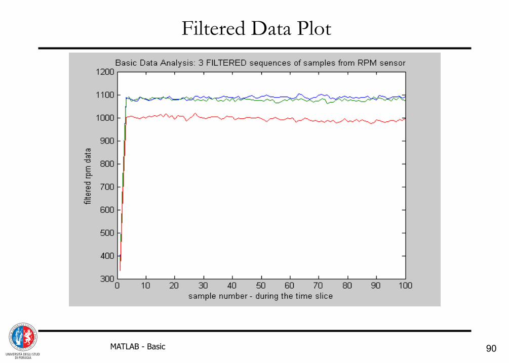
Bin Average Filtering FILTER One-dimensional digital filter. Y = FILTER(B,A,X) filters the data in vector X with the filter described by vectors A and B to create the filtered data Y. The filter is a "Direct Form II Transposed" implementation of the standard difference equation: a(1)*y(n) = b(1)*x(n) + b(2)*x(n-1) + ... + b(nb+1)*x(n-nb) - a(2)*y(n-1) - ... - a(na+1)*y(n-na) >> filter(ones(1,3), 3, rpm_raw) ans = 359 351 335.67 719 724.33 667 1088.3 1081.7 1001 1084 1091.7 1004.7 1081 1073 1006.7

This example uses an FIR filter to compute a moving average using a window size of 3

90 MATLAB - Basic

Filtered Data Plot

91 MATLAB - Basic

Fast Fourier Transform (FFT)

•  fft is one of the built-in functions in MATLAB •  The fft function can compute the discrete Fourier

transform of any arbitrary length sequence. fft incorporates most known fast algorithms for various lengths (e.g. power of 2)

•  Not all lengths are equally fast

92 MATLAB - Basic

Example: FFT of sine Wave in Noise

>> fs = 1000; >> t = [0:999]*(1/fs); >> x = sin(2*pi*250*t); >> X = fft(x(1:512)); >> noise = 0.8*randn(size(x)); >> xn = x + noise; >> XnMag = fftshift(20*log10(abs(fft(xn(1:512))))); >> XnMagPf = XnMag(256:512); >> frq = [0:length(XnMagPf) - 1]'*(fs/length(XnMag)); >> plot(frq, XnMagPf) >> xlabel('freq. (Hz)'); >> ylabel('Mag. (db)');

93 MATLAB - Basic

Frequency Spectrum

Numerical Analysis

95 MATLAB - Basic

Solving Linear Equations

Consider the set of equations Ax = b • A is an n x m matrix, x is an m x 1 vector and b is

an n x 1 vector •  The rank of a matrix is the number of independent

rows (or columns). Rank can be checked using the MATLAB command rank

•  Equations are

• consistent if rank(A) = rank([A b]) •  independent if rank(A) = n

Existence of solution

Uniqueness of solution

96 MATLAB - Basic

Linear Equations, n = m

•  When A is square (i.e., n = m) and the equations

are independent and consistent, the unique solution can be found using the \ operator.

•  MATLAB finds the solution

using a LU decomposition of A.

>> A = [1 2 3; 4 5 6; 7 8 0] A = 1 2 3 4 5 6 7 8 0 >> b = [366; 804; 351] b = 366 804 351 >> [rank(A) rank([A b])] ans = 3 3 >> x = A\b x = 25 22 99

97 MATLAB - Basic

Ordinary Differential Equations

•  MATLAB has a collection of m-files, called the ODE suite to solve initial value problems of the form

M(t,y)dy/dt = f(t, y)

y(t0) = y0

where y is a vector.

•  The ODE suite contains several procedures to solve

such coupled first order differential equations.

98 MATLAB - Basic

Steps in ODE Solution Using MATLAB •  Express the differential equation as a set of first-order ODEs

M(t,y)dy/dt = f(t,y)

•  Write an m-file to compute the state derivative function dydt = myprob(t, y)

•  Use one of the ODE solvers to solve the equations

[t, y] = ode_solver(‘myprob’, tspan, y0);

Time index

Solution matrix

ODE solver

ODE file for

derivatives

Solution time span

[t0 tf]

Initial conditions

99 MATLAB - Basic

ODE Suite Solvers

•  ode23: explicit, one-step Runge-Kutta low-order solver

•  ode45: explicit, one-step Runge-Kutta medium order solver. First solver to try on a new problem

•  ode113: multi-step Adams-Bashforth-Moulton solver of varying order

•  ode23s: implicit, one-step modified Rosenbrock solver of order 2

•  ode15s: implicit, multi-step numerical differentiation solver of varying order. Solver to try if ode45 fails or is too inefficient

Non-stiff equations Stiff equations

100 MATLAB - Basic

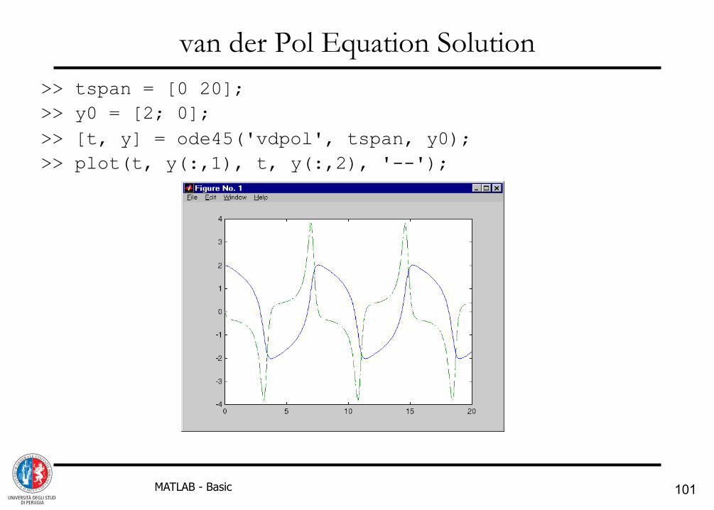
Example : van der Pol Equation

•  Equation is d2x/dt2 - µ(1-x2)dx/dt + x = 0 •  Convert to first order ODEs

using y1 = x, y2 = dx/dt

dy1/dt = y2

dy2/dt=µ(1-y12)y2-y1

function dydt = vdpol(t,y)

%

% van der Pol equation

mu = 2;

dydt = [y(2);mu*(1- … y(1)^2)*y(2)-y(1)];

ODE File vdpol.m

101 MATLAB - Basic

van der Pol Equation Solution >> tspan = [0 20]; >> y0 = [2; 0]; >> [t, y] = ode45('vdpol', tspan, y0); >> plot(t, y(:,1), t, y(:,2), '--');

102 MATLAB - Basic

More on ODE Solvers

•  There are a number of different options in specifying the ODE file. Check HELP on odefile for details.

•  odeset and odeget can be used to set and examine

the ODE solver options. •  Can find events (such as max/min/zero, crossings etc.)

in the solution.

Graphics, Data Visualization & Movies

104 MATLAB - Basic

Overview

•  Plots –  Simple plots –  Subplots (Multiple Axis Regions) –  Mesh plots (Colored wire-frame view of surface) –  Surface Plots –  Patches –  Contour Plots –  Visualization

•  Images –  Indexed images –  Intensity images –  Truecolor images –  Reading and writing images

•  Movies

105 MATLAB - Basic

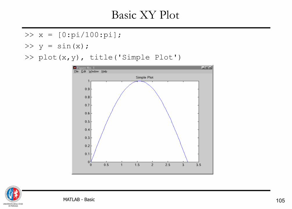
Basic XY Plot

>> x = [0:pi/100:pi];

>> y = sin(x);

>> plot(x,y), title('Simple Plot')

106 MATLAB - Basic

Multiple Curve Plots

Line color, style, marker type, all within single quotes

>> z = cos(x);

>> plot(x,y,'g.',x,z,'b-.'), title('More Complicated')

107 MATLAB - Basic

Plot Power: Contour & 3-D Mesh

To save:

print -djpeg myfigure.jpg

use help print for options

>> t = 0:pi/25:pi; >> [x,y,z] = cylinder(4*cos(t));

>> subplot(2,1,1)

>> contour(y)

>> subplot(2,1,2)

>> mesh(x,y,z)

>> xlabel('x')

>> ylabel('this is the y axis')

>> text(1,-2,0.5,...

'\it{Note the gap!}')

108 MATLAB - Basic

Subplots

Used to display multiple plots in the same figure window, subplot(m,n,i) subdivides the window into m-by-n subregions

(subplots) and makes the ith subplot active for the current plot

>> subplot(2,3,1) >> plot(t, sin(t), 'r:square') >> axis([-Inf,Inf,-Inf,Inf]) >> subplot(2,3,3) >> plot(t, cos(t), 'g') >> axis([-Inf,Inf,-1,1]) >> subplot(2,3,5) >> plot(t, sin(t).*cos(t), 'b-.') >> axis([-Inf,Inf,-Inf,Inf])

4 5 6

2

3 1

109 MATLAB - Basic

Surface Plots

• surf(Z) generates a colored faceted 3-D view of the surface. –  By default, the faces are quadrilaterals, each of constant color,

with black mesh lines –  The shading command allows you to control the view

>> figure(2); >> [X,Y] = meshgrid(-16:1.0:16); >> Z = sqrt(X.^2 + Y.^2 + 5000); >> surf(Z)

>> shading flat

>> shading interp

Default: shading faceted