lecture 5: functions, debugging - b0b17mtb, be0b17mtb matlab

Lecture 5: Functions, DebuggingB0B17MTB, BE0B17MTB – MATLAB

Miloslav Čapek, Viktor Adler, Michal Mašek, and Vít Losenický

Department of Electromagnetic FieldCzech Technical University in Prague

Czech [email protected]

October 11Winter semester 2021/22

B0B17MTB, BE0B17MTB – MATLAB Lecture 5: Functions, Debugging 1 / 73

https://cw.fel.cvut.cz/b211/courses/mtb


mailto:[email protected]



Outline

1. Functions

2. Debugging

3. Excercises


https://www.cvut.cz/en



Functions

Functions in MATLAB

I More efficient, more transparent, and faster than scripts.I Defined input and output, comments → function header is necessary.I Can be called from Command Window, script, or from other function (in all cases the

function has to be accessible).I Each function has its own Workspace created upon the function’s call and terminated

with the last line of the function.I All principles of programming covered at earlier stages of the course (memory allocation,

data type conversion, indexing, etc.) apply also to MATLAB functions.I In case of overloading a built-in function, e.g., defining your own variable/function sum,

builtin function is applicable. Scriptsan

dFu

nction

s





Functions

Function Header

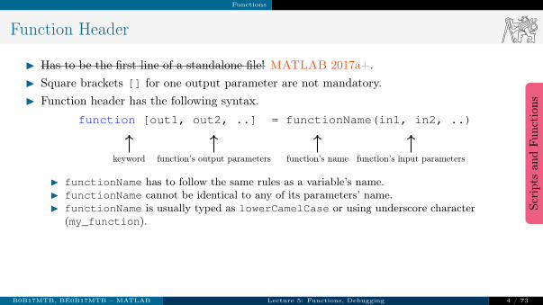
I Has to be the first line of a standalone file! MATLAB 2017a+.I Square brackets [] for one output parameter are not mandatory.I Function header has the following syntax.

function [out1, out2, ..] = functionName(in1, in2, ..)

keyword function’s output parameters function’s name function’s input parameters

I functionName has to follow the same rules as a variable’s name.I functionName cannot be identical to any of its parameters’ name.I functionName is usually typed as lowerCamelCase or using underscore character

(my_function).

Scriptsan

dFu

nction

s





Functions

Simple Example of a Function

I Any function in MATLAB can be called with less input parameters or less outputparameters than stated in the header.I For instance, consider following function:

function [out1, out2, out3] = funcG(in1, in2, in3)

I All following calling syntaxes are correct:[out1, out2] = funcG(in1)funcG(in1, in2, in3)[out1] = funcG(in1, in2, in3)[~, ~, out3] = funcG(in1, in2)

I Another header definitions:function funcA % unusual, but possible, without input and outputfunction funcB(in1, in2) % e.g. function with GUI output, print, etc.function out1 = funcC % data preparation, pseudorandom data, etc.function out1 = funcD(in1) % "proper" functionfunction [out1, out2] = funcE(in1, in2) % proper function with more parameters

Scriptsan

dFu

nction

s





Functions

Calling MATLAB Function

Change Fibonacci script into a function:I Input parameter:

limit (f(end) < limit)I output parameter:

f (Fibonacci sequence)

function f = fibonacci(limit)%% Fibonacci sequencef = [1 1]; pos = 1;while f(pos) + f(pos + 1) < limit

f(pos + 2) = f(pos) + f(pos + 1);pos = pos + 1;

endend

I drawbacks:I Input is not validated.I Matrix f is not allocated, i.e., matrix

keeps growing (slow)

>> f = fibonacci(1000);>> plot(f); grid on;

450





Functions

Comments Inside a Function

Function help displayedupon: » help myFcn1.

1st line (so called H1line), this line is searchedfor by lookfor. Usuallycontains function’s namein capital characters anda brief description of thepurpose of the function.

function [dataOut, idx] = myFcn1(dataIn, method)%MYFCN1: Calculates...% syntax, description of input, output,% expamples of function's call, author, version% other similar functions, other parts of help

matX = dataIn(:, 1);sumX = sum(matX); % sumation%% displaying the result:disp(num2str(sumX));

DO COMMENT!!Comments significantly improve transparency of functions’ code.

Scriptsan

dFu

nction

s





Functions

Function Documentation: Example

Scriptsan

dFu

nction

s





Functions

Simple Example of a Function I.

I Propose a function to calculate length of a belt between two wheels.I Diameters of both wheels d1, d2, are known as well as their distance d (= function’s inputs).I Sketch a draft, analyze the situation and find out what you need to calculate.I Test the function for some scenarios and verify results.I Comment the function, apply commands doc, lookfor, help, type.

100





Functions

Simple Example of a Function II.

I Total length is: L = l1 + 2l2 + l3.I Known diameters → recalculate to radii: r1 = d1/2, r2 = d2/2.

I l2 to be determined using Pythagorean theorem: l2 =

√d2 − (r2 − r1)

2.

I Analogically for ϕ: ϕ = asin

(r2 − r1d

).

I Finally, the arches: l1 = (π − 2ϕ) r1, l3 = (π + 2ϕ) r2.

I Verify your results:d1 = 2, d2 = 2, d = 5L = 2π+2·5 ≈ 16.2832.

d

ϕ

ϕ

ϕ

ϕ

d

r2 − r1

r1

r2

l2

l1 l31 2

500





Functions

Simple Example of a Function III.

function L = band_wheel(d1,d2,d)%% band_wheel: calculation of band-wheellength%% Syntax:% [L] = band_wheel(d1,d2,d);% Example:% L = band_wheel(4,8,12)% Input:% d1 ... diameter of 1st wheel% d2 ... diameter of 2nd wheel% d ... distance between wheels% Output:% L ... length of band-wheel%% ver. 2, 03-2013,[email protected]

r1 = d1/2; % radius of 1st wheelr2 = d2/2; % radius of 2nd wheelL2 = sqrt(d^2 - (r2-r1)^2); % lengthof l2 segmentphi = asin((r2 - r1)/d); % angle phiom1 = pi - 2*phi;om2 = pi + 2*phi;L1 = om1*r1; % length of 1st arcL3 = om2*r2; % length of 2nd arcL = L1 + 2*L2 + L3; % overall lengthend

doc band_wheelhelp band_wheeltype band_wheellookfor band_wheel

Scriptsan

dFu

nction

s





Functions

Workspace of a Function

I Each function has its own workspace.

Scriptsan

dFu

nction

s





Functions

Data Space of a Function

I When calling a function:I Input variables are not copied into workspace of the function, they are just made accessible

for the function (call-by-reference, copy-on-write technique) unless they are modified.I If an input variable is modified inside the function, its value is copied into the function’s

workspace.I If an input variable is also used as an output variable, it is immediately copied.I Beware of using large arrays as input parameters to the functions which are then modifying

them. With respect to memory demands and calculation speed-up, it is preferred to takethe necessary elements out of the array and take care of them separately.

I In the case of the recursive calling of a function, the function’s workspace is created foreach call.I Pay attention to the excessive increase in the number of workspaces.

I Sharing variables between multiple workspaces (global variables) is generally notrecommended and can be avoided in most cases.

Scriptsan

dFu

nction

s





Functions

Function execution

I When is function terminated?I MATLAB interpreter reaches the last line.I Interpreter comes across the keyword return.I Interpreter encounters an error (can be evoked by error as well).I On pressing CTRL+C.

function res = myFcn2(matrixIn)

if isempty(matrixIn)error('matrixInCannotBeEmpty');

endnormMat = matrixIn - max(max(matrixIn));

if matrixIn == 5res = 20;return

endend

Scriptsan

dFu

nction

s





Functions

Number of Input and Output Variables I.

I Number of input and output variables is specified by functions nargin and nargout.I These functions enable to design the function header in a way to enable variable number

of input/output parameters.function [out1, out2] = myFcn3(in1, in2)nArgsIn = nargin;if nArgsIn == 1

% do somethingelseif nArgsIn == 2

% do somethingelse

error('Bad inputs!');end% computation of out1if nargout == 2

% computation of out2endend

Scriptsan

dFu

nction

s





Functions

Number of Input and Output Variables III.a

Modify the function fibonacci.m to enable variable input/output parameters:I It is possible to call the function without input parameters.

I The series is generated in the way that the last element is less than 1000.I It is possible to call the function with one input parameter in1.

I The series is generated in the way that the last element is less than in1.I It is possible to call the function with two input parameters in1, in2.

I The series is generated in the way that the last element is less than in1 and at the sametime the first 2 elements of the series are given by vector in2.

I It is possible to all the function without output parameters or with one outputparameter.I The generated series is returned.

I It is possible to call the function with two output parameters.I The generated series is returned together with an object of class Line, which is plotted in a

graph: hLine = plot(f);. 500





Functions

Number of Input and Output Variables III.b

function [out1, out2] = fibonacciFcn(in1, in2)% documentation is here!!!nArgIn = nargin;if nArgIn == 0

limit = 1e3;f = [0, 1];

elseif nArgIn == 1limit = in1;f = [0, 1];

elseif nArgIn == 2limit = in1;f = in2;

end

n = 1; % index for series generationwhile f(n+1) < limit

f(n+2) = f(n) + f(n+1);n = n + 1;

endf(end) = [];

out1 = f;if nargout == 2

out2 = plot(f);endend





Functions

Syntactical Types of Functions

Function type Descriptionmain The only one in the m-file visible from outside, above principles apply.local All functions in the same file except the main function, accessed by the

main function, has its own workspace, can be placed into [private]folder to preserve the private access, function in script file (2016b+).

nested The function is placed inside the main function or local function, seesthe WS of all superior functions.

handle Function reference (mySinX = @sin).anonymous Similar to handle functions (myGFcn = @(x) sin(x) + cos(x)).OOP Class methods with specific access, static methods.

I Any function in MATLAB can launch a script which is then evaluated in the workspaceof the function that launched it, not in the base workspace of MATLAB (as usual).

I The order of local functions is not important (logical connection!).I Help of local functions is not accessible using help.

Scriptsan

dFu

nction

s





Functions

Local Functions I.

I Local functions launched by a main function. TheyI can (should) be terminated with the keyword end,I are used for repeated tasks inside the main function (helps to simplify the problem by

decomposing it into simple parts),I “see” each other and have their own workspace,I are often used to process graphical elements’ events (callbacks) when developing GUI.

function PRx = getRxPower(R, PTx, GAnt, freq)% main function bodyFSL = computeFSL(R, freq); % free-space lossPRx = PTx + 2*GAnt - FSL; % received powerend

function FSL = computeFSL(R, freq)% local function bodyc0 = 3e8;lambda = c0./freq;FSL = 20*log10(4*pi*R./lambda);end

Scriptsan

dFu

nction

s





Functions

Local Functions II.

I Local functions launched by a script (new from R2016b). TheyI have to be at the end of file,I have to be terminated with the keyword end,I “see” each other and have their own workspace,I are not accessible outside the script file.

clear;% start of scriptr = 0.5:5; % radii of circlesareaOfCirles = computeArea(r);

function A = computeArea(r)% local function in scriptA = pi*r.^2;end

Scriptsan

dFu

nction

s





Functions

Local Functions III.

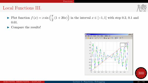
I Plot function f (x) = x sin(π

2(1 + 20x)

)in the interval x ∈ [−1, 1] with step 0.2, 0.1 and

0.01.I Compare the results!

close all; clear; clc[x1, f1] = myFunc(-1:0.2:1);[x2, f2] = myFunc(-1:0.1:1);[x3, f3] = myFunc(-1:0.01:1)

figure;hold on; grid on;plot(x1, f1, 'r');plot(x2, f2, 'g');plot(x3, f3, 'b');legend('0.2', '0.1', '0.01');

function [x, f] = myFunc(x)f = x .* sin(pi/2*(1+20*x));

end

300





Functions

Nested Functions

I Nested functions are placed inside other functions.I In enables us to use workspace of the parent function and to efficiently work with (usually

small) workspace of the nested function.I Functions can not be placed inside conditional/loop control statements

(if-elseif-else/switch-case/for/while/try-catch).

function x = A(p)% single% nested function..

function y = B(q)..end

..end

function x = A(p)% more% nested functions..

function y = B(q)..end

function z = C(r)..end

..end

function x = A(p)% multiple% nested function..

function y = B(q)..function z = C(r)..end

..end

..end

Scriptsan

dFu

nction

s





Functions

Nested Functions: Calling

I Apart from its workspace, nestedfunctions can also access workspaces of allfunctions it is nested in.

I Nested functions can be called from:I its parent function,I nested functions on the same level of

nesting,I function nested in it.

I It is possible to create handle to a nestedfunction.I See later.

function x = A(p)function y = B(q)..

function z = C(t)..end

end..

function u = D(r)..

function v = E(s)..end

..end

..end

Scriptsan

dFu

nction

s





Functions

Private Functions

I They are basically the local functions, and they can be called by all functions placed inthe root folder.

I Reside in sub-folder [private] of the main function.I Private functions can be accessed only by functions placed in the folder immediately

above that private sub-folder.I [private] is often used with larger applications or in the case where limited visibility of

files inside the folder is desired.

...\TCMapp

private\

eigFcn.m

impFcn.m

rwgFcn.m

parTCM.m

preTCM.m

These functions can be calledby parTCM.m and preTCM.monly.

parTCM.m calls functions in[private].

Scriptsan

dFu

nction

s





Functions

Handle Functions

I It is not a function as such.I Handle = reference to a given function.

I Properties of a handle reference enable to call a function that is otherwise not visible.I Reference to a handle (here fS) can be treated is a usual way.

I Typically, handle references are used as input parameters of functions.>> fS = @sin; % handle creation>> fS(pi/2)ans =

1

Scriptsan

dFu

nction

s





Functions

Anonymous functions I.

I Anonymous functions make it possible to create handle reference to a function that is notdefined as a standalone file.I The function has to be defined as one executable expression.

>> sqr = @(x) x.^2; % create anonymous function (handle)>> res = sqr(5); % x ~ 5, res = 5^2 = 25;

I Anonymous function can have more input parameters.>> A = 4; B = 3; % parameters A,B have to be defined>> sumAxBy = @(x, y) (A*x + B*y); % function definition>> res2 = sumAxBy(5,7); % x = 5, y = 7% res2 = 4*5+3*7 = 20+21 = 41

I Anonymous function stores variables required as well as prescription.

I » doc Anonymous Functions

>> Fcn = @(hndl, arg) (hndl(arg))>> res = Fcn(@sin, pi)

>> A = 4;>> multAx = @(x) A*x;>> clear A>> res3 = multAx(2);% res3 = 4*2 = 8

Scriptsan

dFu

nction

s





Functions

Anonymous functions II.

I Create anonymous function A (p) = [A1 (p) A2 (p) A3 (p)] so that

A1 (p) = cos2 (p) ,

A2 (p) = sin (p) + cos (p) ,

A3 (p) = 1.

I Calculate and display its components for range p = [0, 2π].

A = @(p) [cos(p).^2, sin(p)+cos(p), 1*ones(size(p))]p = linspace(0, 2*pi).';plot(p, A(p));

I Check the function A (p) with MATLAB built-in function functions, i.e.,functions(A).

500





Functions

Functions: Advanced Techniques

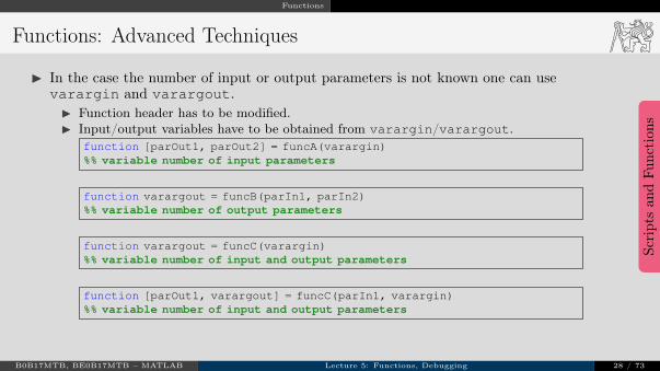
I In the case the number of input or output parameters is not known one can usevarargin and varargout.I Function header has to be modified.I Input/output variables have to be obtained from varargin/varargout.

function [parOut1, parOut2] = funcA(varargin)%% variable number of input parameters

function varargout = funcB(parIn1, parIn2)%% variable number of output parameters

function varargout = funcC(varargin)%% variable number of input and output parameters

function [parOut1, varargout] = funcC(parIn1, varargin)%% variable number of input and output parameters

Scriptsan

dFu

nction

s





Functions

varargin Function

I Typical usage: functions with many optional parameters/attributes.I e.g., visualisation (functions like stem, surf etc. include varargin)

I Variable varargin is always of type cell (see later), even when it contains just singleitem.

I Function nargin in the body of a function returns the number of input parameters uponthe function’s call.

I Function nargin(fx) returns number of input parameters in function’s header.I When varargin is used in function’s header, returns negative value.

function plot_data(varargin)nargincelldisp(varargin)

par1 = varargin{1};par2 = varargin{2};

Scriptsan

dFu

nction

s





Functions

varargout Function

I Variable number of output variables.I Principle analogical to varargin function.

I Bear in mind that function’s output variables are of type cell.

I Used occasionally.function [s, varargout] = sizeout(x)nout = max(nargout, 1) - 1;s = size(x);for k = 1:nout

varargout{k} = s(k);end

>> [s, rows, cols] = sizeout(rand(4, 5, 2))% s = [4 5 2], rows = 4, cols = 5

Scriptsan

dFu

nction

s





Functions

Advanced Anonymous Functions

I Inline conditional:>> iif = @(varargin) varargin{2*find([varargin{1:2:end}], 1, 'first')}();

I Usage:>> min10 = @(x) iif(any(isnan(x)), 'Don''t use NaNs', ...

sum(x) > 10, 'This is ok', ...sum(x) < 10, 'Sum is low')

>> min10([1 10]) % ans = 'This is ok'>> min10([1 nan]) % ans = 'Don't use NaNs'

I Map:>> map = @(val, fcns) cellfun(@(f) f(val{:}), fcns);

I Usage:>> x = [3 4 1 6 2];>> values = map({x}, {@min, @sum, @prod})>> [extreme, indices] = map({x}, {@min, @max})

Scriptsan

dFu

nction

s





Functions

Variable Number of Input Parameters

I Input arguments are usually inpairs.

I Example of setting of severalparameters to line object.

I For all properties see » docline.

Property ValueColor [RGB]

LineWidth 0.1 - ...Marker ’o’, ’*’, ’x’, ...

MarkerSize 0.1 - ......

>> plot_data(magic(3),...'Color',[.4 .5 .6],'LineWidth',2);

>> plot_data(sin(0:0.1:5*pi),...'Marker','*','LineWidth',3);

function plot_data(data, varargin)if isnumeric(data) && ~isempty(data)

hndl = plot(data);else

fprintf(2, ['Input variable ''data''', ...'is not a numerical variable.']);

return;end

while length(varargin) > 1set(hndl, varargin{1}, varargin{2});varargin(1:2) = [];

endend

Scriptsan

dFu

nction

s





Functions

Output Parameter varargout

I Modify the function fibonacciFcn.m so that it has only one output parametervarargout and its functionality was preserved.

function varargout = fibonacciFcn2(in1, in2)% documentation is here!!!nArgIn = nargin;if nArgIn == 0

limit = 1e3;f = [0, 1];

elseif nArgIn == 1limit = in1;f = [0, 1];

elseif nArgIn == 2limit = in1;f = in2;

end

n = 1; % index for series generationwhile f(n+1) < limit

f(n+2) = f(n) + f(n+1);n = n + 1;

endf(end) = [];varargout{1} = f;if nargout == 2

varargout{2} = plot(f);end

180





Functions

Expression Evaluated in Another Workspace

I Function evalin (“evaluate in”) can be used to evaluate an expression in a workspacethat is different from the workspace where the expression exists.

I part from current workspace, other workspaces can be used as wellI 'base': base workspace of MATLAB.I 'caller': workspace of parent function (from which the function was called).

I Can not be used recursively.

>> clear; clc;>> A = 5;>> res = eval_in% res = 12.7976

function out = eval_in%% no input parameters (A isn't known here)

k = rand(1,1);out = evalin('base', ['pi*A*', num2str(k)]);end

Scriptsan

dFu

nction

s





Functions

Recursion

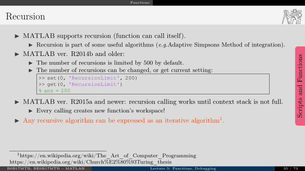
I MATLAB supports recursion (function can call itself).I Recursion is part of some useful algorithms (e.g.Adaptive Simpsons Method of integration).

I MATLAB ver. R2014b and older:I The number of recursions is limited by 500 by default.I The number of recursions can be changed, or get current setting:

>> set(0, 'RecursionLimit', 200)>> get(0, 'RecursionLimit')% ans = 200

I MATLAB ver. R2015a and newer: recursion calling works until context stack is not full.I Every calling creates new function’s workspace!

I Any recursive algorithm can be expressed as an iterative algorithm1.

Scriptsan

dFu

nction

s

1https://en.wikipedia.org/wiki/The_Art_of_Computer_Programminghttps://en.wikipedia.org/wiki/Church%E2%80%93Turing_thesis





Functions

Number of Recursion Steps

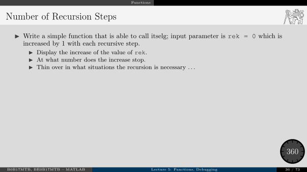
I Write a simple function that is able to call itselg; input parameter is rek = 0 which isincreased by 1 with each recursive step.I Display the increase of the value of rek.I At what number does the increase stop.I Thin over in what situations the recursion is necessary . . .

function out = test_function(rek)%% for testing purposes

rek = rek + 1out = test_function(rek);end

>> test_function(0)

360





Functions

MATLAB Path

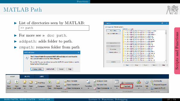
I List of directories seen by MATLAB:>> path

I For more see » doc path.I addpath: adds folder to path.I rmpath: removes folder from path

Scriptsan

dFu

nction

s





Functions

Namespace

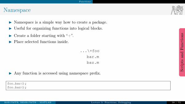
I Namespace is a simple way how to create a package.I Useful for organizing functions into logical blocks.

I Create a folder starting with “+”.I Place selected functions inside.

...\+foo

bar.m

baz.m

I Any function is accessed using namespace prefix.

foo.bar();foo.baz();

Scriptsan

dFu

nction

s





Functions

Order of Function Calling

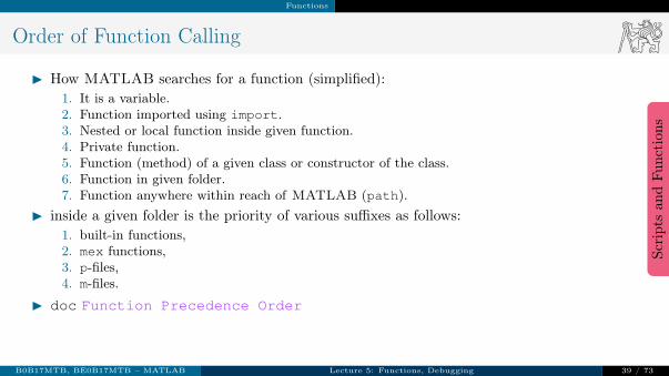
I How MATLAB searches for a function (simplified):1. It is a variable.2. Function imported using import.3. Nested or local function inside given function.4. Private function.5. Function (method) of a given class or constructor of the class.6. Function in given folder.7. Function anywhere within reach of MATLAB (path).

I inside a given folder is the priority of various suffixes as follows:1. built-in functions,2. mex functions,3. p-files,4. m-files.

I doc Function Precedence Order

Scriptsan

dFu

nction

s





Functions

Class inputParser I.

I Enables to easily test input parameters of a function.I It is especially useful to create functions with many input parameters with pairs

'parameter', value.I Very typical for graphical functions.

>> x = -20:0.1:20;>> fx = sin(x)./x;>> plot(x, fx, 'LineWidth', 3, 'Color', [0.3 0.3 1], 'Marker', 'd',...'MarkerSize', 10, 'LineStyle', ':')

I Method addParameter enables to insert optional parameter.I Initial value of the parameter has to be set.I The function for validity testing is not required.

I Method addRequired defines name of mandatory parameter.I On function call it always has to be entered at the right place.

Scriptsan

dFu

nction

s





Functions

Class inputParser II.

I Following function plots a circle or a square of defined size, color and line width.function drawGeom(dimension, shape, varargin)p = inputParser; % instance of inputParserp.CaseSensitive = false; % parameters are not case sensitivedefaultColor = 'b'; defaultWidth = 1;expectedShapes = {'circle', 'rectangle'};validationShapeFcn = @(x) any(ismember(expectedShapes, x));p.addRequired('dimension', @isnumeric); % required parameterp.addRequired('shape', validationShapeFcn); % required parameterp.addParameter('color', defaultColor, @ischar); % optional parameterp.addParameter('linewidth', defaultWidth, @isnumeric) % optional parameterp.parse(dimension, shape, varargin{:}); % parse input parameters

switch shapecase 'circle'

figure;rho = 0:0.01:2*pi;plot(dimension*cos(rho), dimension*sin(rho), ...

p.Results.color, 'LineWidth', p.Results.linewidth);axis equal;

case 'rectangle'figure;plot([0 dimension dimension 0 0], ...

[0 0 dimension dimension 0], p.Results.color, ...'LineWidth', p.Results.linewidth)

axis equal;end

Scriptsan

dFu

nction

s





Functions

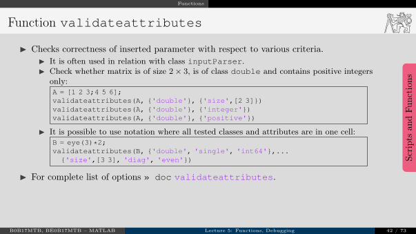
Function validateattributes

I Checks correctness of inserted parameter with respect to various criteria.I It is often used in relation with class inputParser.I Check whether matrix is of size 2× 3, is of class double and contains positive integers

only:A = [1 2 3;4 5 6];validateattributes(A, {'double'}, {'size',[2 3]})validateattributes(A, {'double'}, {'integer'})validateattributes(A, {'double'}, {'positive'})

I It is possible to use notation where all tested classes and attributes are in one cell:B = eye(3)*2;validateattributes(B, {'double', 'single', 'int64'},...{'size',[3 3], 'diag', 'even'})

I For complete list of options » doc validateattributes.

Scriptsan

dFu

nction

s





Functions

Original Names of Input Variables

I Function inputname makes it possible to determine names of input parameters ahead offunction call.I Consider folowing function call:

>> y = myFunc1(xdot, time, sqrt(25));

I And then inside the function:function output = myFunc1(par1, par2, par3)

% ...p1str = inputname(1); % p1str = 'xdot';p2str = inputname(2); % p2str = 'time';P3str = inputname(3); % p3str = '';% ... Sc

riptsan

dFu

nction

s





Functions

Advanced example of a Function I.a

I Write a function that implements the array binary search.I Input parameters are array (sorted array) and value (searched value).I Output parameter pos is the position in the array. If the value is not there pos = -1.





Functions

Advanced example of a Function I.b

Algorithm 1: Pseudocode of an implementation of the Binary searchDetermine the outer bounds l and r of the array A.while Left bound <= Right bound doSet the middle element mif Am = searched value thenReturn m.

else if Am < searched value thenSet the left bound to m+ 1.

else if Am > searched value thenSet the right bound to m− 1.

end ifend whileIndicate failure of the search. Return -1.

500





Functions

Advanced example of a Function I.c

function pos = binarySearch(array, value)left = 1;right = length(array);while left <= right

mid = left + round((right - left)/2);if array(mid) == value

pos = mid;return

elseif array(mid) < valueleft = mid + 1;

elseright = mid - 1;

endendpos = -1;end





Functions

Function and m-file Dependence

I Identify all the files and functions required for sharing your code.I Function matlab.codetools.requiredFilesAndProducts

I returns user files and products necessary for evaluation of a function/script,I does not return which are part of required products.

I Dependencies of Homework1 checker:

[fList, plist] = matlab.codetools.requiredFilesAndProducts('homework1')fList =1x5 cell array{'C:\Homework1\homework1.m'}{'C:\Homework1\problem1A.m'}{'C:\Homework1\problem1B.m'}{'C:\Homework1\problem1C.m'}{'C:\Homework1\problem1D.m'}

plist =struct with fields:

Name: 'MATLAB'Version: '9.4'

ProductNumber: 1Certain: 1

Program

Flow





Functions

Function why

I It is a must to try that one!I Try help why.I Try to find out how many answers exist.

Scriptsan

dFu

nction

s





Functions

Script startup.m

I Script startup.m:I Is always executed at MATLAB start-up.I It is possible to put your predefined constant and other operations to be executed(loaded)

at MATLAB start-up.I Location (use which startup):

I ...\Matlab\R20XXx\toolbox\local\startup.m

I Change of base folder after MATLAB start-up:%% script startup.m in ..\Matlab\Rxxx\toolbox\local\clc;disp('Workspace is changed to: ');cd('d:\Data\Matlab');cddisp(datestr(now, 'mmmm dd, yyyy HH:MM:SS.FFF AM'))

Scriptsan

dFu

nction

s





Debugging

Debugging I.

I Bug → debugging.I We distinguish:

I Semantic errors (“logical” or “algorithmic” errors).I Usually difficult to identify.

I Syntax errors (“grammatical” errors).I Pay attention to the content of error messages – it makes error elimination easier.

I Unexpected events (see later).I For example, a problem with writing to open file, not enough space on disk etc.

I Rounding errors (everything is calculated as it should be but the result is wrong anyway).I It is necessary to analyze the algorithm in advance, to determine the dynamics of calculation

etc.

I Software debugging and testing is an integral part of software development.I Later we will discuss the possibilities of code acceleration using MATLAB profile.

Scriptsan

dFu

nction

s





Debugging

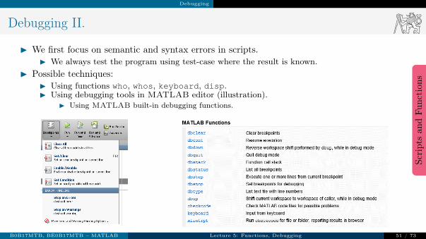
Debugging II.

I We first focus on semantic and syntax errors in scripts.I We always test the program using test-case where the result is known.

I Possible techniques:I Using functions who, whos, keyboard, disp.I Using debugging tools in MATLAB editor (illustration).

I Using MATLAB built-in debugging functions.

Scriptsan

dFu

nction

s





Debugging

Useful Functions for Script Generation

I The function keyboard stops execution of the code and gives control to the keyboard.I The function is widely used for code debugging as it stops code execution at the point

where any doubts about the code functionality existK>>

I keyboard status is indicated by K» (K appears before the prompt).I The keyboard mode is terminated by dbcont or press F5 (Continue).

I Function pause halts code execution.I pause(x) halts code execution for x seconds.

% code; code; codepause;

I See also: echo, waitforbuttonpress.I Special purpose functions.

Scriptsan

dFu

nction

s





Debugging

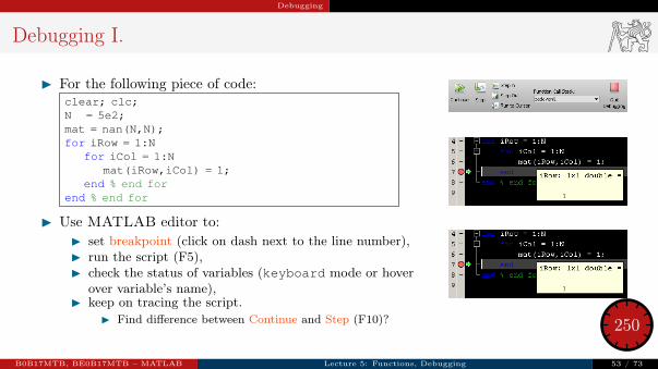
Debugging I.

I For the following piece of code:clear; clc;N = 5e2;mat = nan(N,N);for iRow = 1:N

for iCol = 1:Nmat(iRow,iCol) = 1;

end % end forend % end for

I Use MATLAB editor to:I set breakpoint (click on dash next to the line number),I run the script (F5),I check the status of variables (keyboard mode or hover

over variable’s name),I keep on tracing the script.

I Find difference between Continue and Step (F10)? 250





Debugging

Advanced Debugging

I Conditional breakpoints:I Serve to suspend the execution of code when a condition is fulfilled.

I Sometimes, the set up of the correct condition is not an easy task . . .I Easier to find errors in loops.

I Code execution can be suspended in a particular loop.

I The condition may be arbitrary evaluable logical expression.% code with an errorclear; clc;N = 100;mat = magic(2*N);selection = zeros(N, N);for iRow = 1:N+2

selection(iRow, :) = ...mat(iRow, iRow:N+iRow-1);

end

Scriptsan

dFu

nction

s





Debugging

Selected Hints for Code Readability I.

I Use indention of loop’s body, indention of code inside conditions(TAB).I Size of indention can be adjusted in preferences (usually 3 or 4 spaces).

I Use “positive” conditions.I i.e.use isBigger or isSmaller, not isNotBigger (can be confusing).

I Complex expressions with logical and relation operators should be evaluated separately→ higher readability of code.I Compare:

if (val>lowLim)&(val<upLim)&~ismember(val,valArray)% do something

end

isValid = (val > lowLim) & (val < upLim);isNew = ~ismember(val, valArray);if isValid & isNew

% do somethingend

Scriptsan

dFu

nction

s





Debugging

Selected Hints for Code Readability II.

I Code can be separated with a blank line to improve clarity.I Use two lines for separation of blocks of code.

I Alternatively use cells or commented lines, for example:% ---------

I Consider to use of spaces to separate operators (=, &, |).I To improve code readability:

(val>lowLim)&(val<upLim)&~ismember(val,valArray)

I vs.(val > lowLim) & (val < upLim) & ~ismember(val, valArray)

I In the case of nesting use comments placed after end. Scriptsan

dFu

nction

s





Debugging

Useful Tools for Long Functions

I Bookmarks:I CTRL+F2 (add/remove

bookmark),I F2 (next bookmark),I SHIFT+F2 (previous

bookmark).I Go to . . .

I CTRL+G (go to line).I Long files can be split.

I Same file can be openede.g.twice.

bookmarks

Scriptsan

dFu

nction

s





Debugging

Function publish I.

I Serves to create script, function or class documentation.I Provides several output formats (html, doc, ppt, LATEX, . . . ).I Help creation (» doc my_fun) directly in the code comments!

I Provides wide scale of formatting properties(titles, numbered lists, equations, graphicsinsertion, references, . . . ).

I Enables to insert print screens into documentation.I Documented code is implicitly launched on publishing.

I Supports documentation creation directly from editor menu:

Scriptsan

dFu

nction

s





Debugging

Function publish II.%% Solver of Quadratic Equation% Function *solveQuadEq* solves quadratic equation.%% Theory% A quadratic equation is any equation having the form% $ax^2+bx+c=0$% where |x| represents an unknown, and |a|, |b|, and |c|% represent known numbers such that |a| is not equal to 0.%% Head of function% All input arguments are mandatory!function x = solveQuadEq(a, b, c)%%% Input arguments are:%%% * |a| - _qudratic coefficient_% * |b| - _linear coefficient_% * |c| - _free term_%% Discriminant computation% Gives us information about the nature of roots.D = b^2 - 4*a*c;%% Roots computation% The quadratic formula for the roots of the general% quadratic equation:%% $$x_{1,2} = \frac{ - b \pm \sqrt D }{2a}.$$%% Matlab code:%%x(1) = (-b + sqrt(D))/(2*a);x(2) = (-b - sqrt(D))/(2*a);%%% For more information visit <http://elmag.org>.

publish

Scriptsan

dFu

nction

s





Excercises

Exercises




Excercises

Exercise I.

I Using integral function calculate integral of a function G =

∫g (x) dt in the interval

t ∈ [0, 1] s. The function has following time dependency, where f = 50Hz.

g (t) = 10 cos (2πft) + 5 cos (4πft)

I Solve the problem using handle function.

t = 0:0.001:1;g = my_func(t);plot(t, I)myFunc_hndl = @my_func;G = integral(myFunc_hndl, t(1), t(end))

function I = my_func(t)f = 50;I = 10*cos(2*pi*f*t) +5*cos(4*pi*f*t);end

I Solve the problem using anonymous function.

clear; close all; clc;t_min = 0; t_max = 1;f = 50;g_hndl = @(t) 10*cos(2*pi*f*t) + 5*cos(4*pi*f*t);G = integral(g_hndl, t_min, t_max)

600





Excercises

Exercise II.a

I Find the unknown x in equation f (x) = 0 using Newton’s method.I Typical implementation steps:

I Mathematical model.I Size the problem, its formal solution.

I Pseudocode.I Layout of consistent and efficient code.

I MATLAB code.I Transformation into MATLAB’s syntax.

I Testing.I Usually using a problem with known (analytic) solution.I Try other examples . . .





Excercises

Exercise II.b

I Find the unknown x in equation of type f (x) = 0.I Use Newton’s method.

I Newton’s method:

x

y

f (x)

0 xkxk+1

f (xk)

f ′ (x) =∆f

∆x≈ df

dx

f ′ (x) =∆f

∆x=f (xk − 0)

xk − xk+1

xk+1 = xk −f (xk)

f ′ (xk)

xkxk+1

f (x)





Excercises

Exercise II.c

I Find the unknown x in equation of type f (x) = 0.I Pseudocode:

Algorithm 2: Pseudocode of an implementation of the Newton’s Methodwhile |(xk+1 − xk) /xk| ≥ error and simultaneously k < 20 do

xk+1 = xk −f (xk)

f ′ (xk)display [k xk+1 f (xk+1)]k = k + 1

end while

I Pay attention to correct condition of the (while) cycle.I Create a new function to evaluate f (x) and f ′ (x).I Use following numerical difference scheme to calculate f ′ (x):

f ′ (x) ≈ ∆f =f (xk + ∆)− f (xk −∆)

2∆.





Excercises

Exercise II.d

I Find the unknown x in equation of type f (x) = 0.I Implement the above metnod in MATLAB to find the unknown x in x3 + x− 3 = 0.I This method comes in the form of a script calling following function:

function fx = optim_fcn(x)fx = x^3 + x - 3;end

clear; close all; clc;% enter variables% xk, xk1, err, k, delta

while (cond1 and_simultaneously cond2)% get xk from xk1% calculate f(xk)% calculate df(xk)% calculate xk1% display results% increase value of k

end600





Excercises

Exercise II.e

clear; close all; clc;

xk1 = 5;err = 0.0001;xk = 10*xk1/(1+err);k = 1;K = 20;while (abs((xk1-xk)/xk) >= err) && (k < K)

xk = xk1;fx = optim_fcn(xk);delta = 10*eps(xk);dfx = (optim_fcn(xk + delta) - optim_fcn(xk - delta))/(2*delta);xk1 = xk - fx/dfx;disp([k xk1 fx]);k = k + 1;

end

I What are the limitations of Newton’s method.I In relation with existence of multiple roots.

I Is it possible to apply the method to complex values of x?B0B17MTB, BE0B17MTB – MATLAB Lecture 5: Functions, Debugging 66 / 73




Excercises

Exercise III.

I Modify Newton’s method in the way that the polynomial is entered in the form of ahandle function.I Verify the code by finding roots of a following polynomials: x− 2 = 0, x2 = 1.I Verify the result using function roots.

function [x0, k] = newton_method(xk1, fcn, err, K)xk = 10*xk1/(1+err); % error high enough so the while cycle is enteredk = 1; % first stepwhile (abs((xk1-xk)/xk) >= err) && (k < K)

xk = xk1;delta = 10*eps(xk);fx = feval(fcn, xk);dfx = (feval(fcn, xk + delta) - feval(fcn, xk-delta)) / (2*delta);xk1 = xk - fx/dfx;disp([k xk1 fx]);k = k + 1;

endx0 = xk1;end

600





Excercises

Exercise IV.a

I Expand exponential function using Taylor series:I In this case is is in fact Maclaurin series (expansion about 0).

ex =∞∑

n=0

xn

n!= 1 + x +

x2

2+

x3

6+

x4

24+ . . .

I Compare with result obtained using exp(x).I Find out the deviation in % (what is the base, i.e., 100%?).I Find out the order of expansion for deviation to be lower than 1%.

I Implement the code as a function.I Choose the appropriate name for the function.I Input parameters of the functions are: x (function argument) and N (order of the series).I Output parameters are values: f1 (result of the series), f2 (result of exp(x)) and err

(deviation in %).I Add appropriate comment to the function (H1 line, inputs, outputs).I Test the function! 600





Excercises

Exercise IV.b

function [f1, f2, err] = exp_approx(x, N)%% exp_approx: calculates an aproximation of exp(x)% [f1, f2, err] = exp_approx(x,N)% x ... function argument, N ... order of approximation% f1 ... calculated value% f2 ... "exact" value (given by built-in function)% err ... relative error% example: [fa, fp] = exp_approx(4, 30);

n = 0:N;f = (x.^n)./factorial(n); % it is vectorizedf1 = sum(f); % approximative valuef2 = exp(x); % exact valueerr = 100*abs(1 - f1/f2); % relative error (in [%])end





Excercises

Exercise IV.c

I Create a script to call the above function (with various N).I Find out accuracy of the approximation for x = 0.9, n ∈ {1, . . . , 10}.I Plot the resulting progress of the accuracy (error as a function of n).

clear; close all;Order = 1:10;x = 0.9;Error = zeros(size(Order));for mErr = 1:length(Order)

[~, ~, Error(mErr)] =exp_approx(x, Order(mErr));endplot(Order, Error);% semilogy(Order, Error);xlabel('N (-)'); ylabel('Error(%)');

x = 0.9, n ∈ {1, . . . , 10}





Excercises

Example V.a

I Write a function that approximates definite integral by trapezoidal rule.I Trapezoidal rule:

Sk Sk+1 Sk+2

x

y

f (x)

0 xk xk+1 . . .

f(xk)

f(xk+1)

b∫a

f (x) dx ≈

≈N−1∑n=1

f (xn) + f (xn+1)

2∆xn

xk xk+1

f (xk)

f (xk+1)





Excercises

Example V.b

I Implement a function that approximates definite integral of a function given by handlefunction.I Choose the appropriate name for the function.I Input parameters are f (anonymous function), a (lower limit), b (upper limit) and N

(number of divisions).I Output parameter is I (value of the integral).I Test the function.

I Compare the results with function integral for: f (x) =√

2x + 1; x ∈ [0, 5].

f = @(x) sqrt(2.^x + 1);I = integral_approx(f, 0, 5, 10)integral(f, 0, 5)

function I = integral_approx(f, a, b,N)x = linspace(a, b, N + 1);fx = f(x);S = (fx(1:end-1) + fx(2:end)) .* ...

(x(2:end) - x(1:end-1));I = 0.5 * sum(S);end

600





Questions?B0B17MTB, BE0B17MTB – MATLAB

[email protected]

October 11Winter semester 2021/22

This document has been created as a part of B0B17MTB course.Apart from educational purposes at CTU in Prague, this document may be reproduced, stored, or transmittedonly with the prior permission of the authors.Acknowledgement: Filip Kozák, Pavel Valtr.




mailto:[email protected]



lecture 5: functions, debugging - b0b17mtb, be0b17mtb matlab

Documents