Influence of grain shape on the mechanical behaviour of granular materials

K. Szarf, G. Combe∗, P. Villard

Universite de Grenoble - Laboratoire Sols, Solides, Structures - Risques (3S-R, UJF-INPG-CNRS UMR 5521) DomaineUniversitaire BP53 38041 Grenoble Cedex 9 - France

Abstract

We performed series of numerical vertical compression tests on assemblies of 2D granular material using aDiscrete Element code and studied the results in regard to the grain shape. The samples consist of 5000grains made either of 3 overlapping discs (clump - grain with concavities) or of six-edged polygons (convexgrain). These two types of grains have a similar external envelope, ruled with a geometrical parameter α.In the paper the applied numerical procedure is briefly described followed by the description of the granularmodel used. Observations and mechanical analysis of dense and loose granular assemblies under isotropicloading are made. The mechanical response of our numerical granular samples is studied in the framework ofthe classical vertical compression test with constant lateral stress (biaxial test). The macroscopic responsesof dense and loose samples with various grain shapes comparison show that the shear resistance of a samplemade of clumps increase with the grains concavity. Dense samples made of polygons are less dependant onthe particle shape. This observation is not valid for loose samples made of polygons. The micromechanicalorigins of these results are explored by contact analysis, focusing especially on dense samples made ofclumps: grain concavity furthers particles imbrications and increase shear resistance. Finally we presentsome remarks concerning the kinematics of the deformed samples. Whereas polygon samples submitted to avertical compression present large damage zones (whatever polygons shape), dense samples made of clumpsalways exhibit thin reflecting shear zones caused by clump imbrications only, even if our granular model iscohesionless.This work was done as a part of CEGEO research project1

Key words: DEM, grains shape, clumps of discs, polygons, isotropic compression, vertical compression,friction angle, shear localisationPACS: 04.60.Nc, 81.05.Rm, 45.70.-n

1. Introduction

A typical numerical approach to discrete element modelling of granular materials is to use simple forms ofparticles (discs in 2D [1] or spheres in 3D [2]). Although the computation time is short that way, these modelsare not able to reflect some of the more complex aspects of real granular media behaviour, such as highshear resistance or high volumetric changes [3]. In order to model it properly either numerical parameters(intergranular rolling resistance [4, 5, 6]) or other grain shapes (aggregate of spheres [7] or polyhedral grains[8]) have to be used. The influence of grain shape is not fully understood yet. In this paper we wanted topresent our investigations concerning the influence of grain shape on the mechanical behaviour of granularassemblies, grain concavity in particular. We compared two groups of grains - convex irregular polygonsand non-convex clumps made of three overlapping discs.

1www.granulo-science.org/CEGEO∗Corresponding authorEmail address: gael.combe@ujf-grenoble.fr (G. Combe)

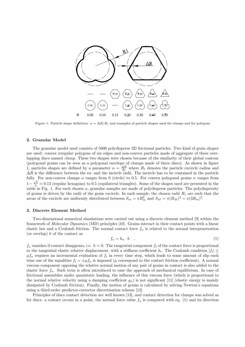
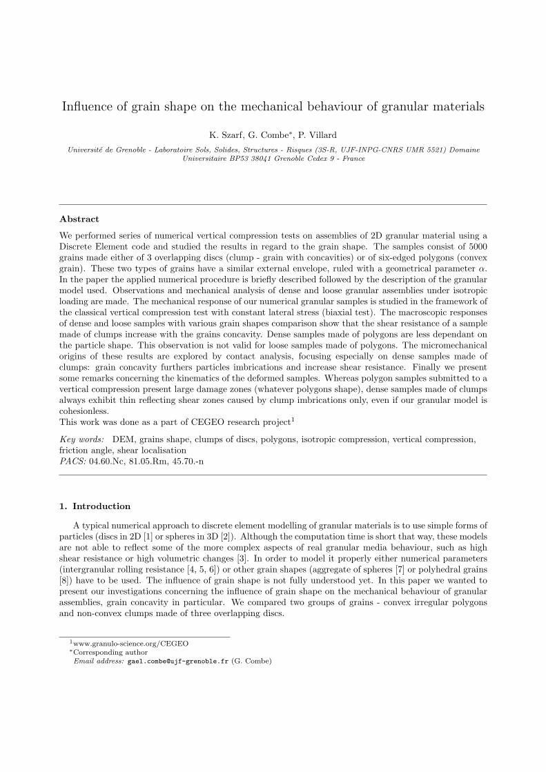
Figure 1: Particle shape definition: α = ∆R/R1 and examples of particle shapes used for clumps and for polygons

2. Granular Model

The granular model used consists of 5000 polydisperse 2D frictional particles. Two kind of grain shapesare used: convex irregular polygons of six edges and non-convex particles made of aggregate of three over-lapping discs named clump. These two shapes were chosen because of the similarity of their global contour(polygonal grains can be seen as a polygonal envelope of clumps made of three discs). As shown in figure1, particles shapes are defined by a parameter α = ∆R

R1

where R1 denotes the particle excircle radius and∆R is the difference between the ex- and the incircle radii. The incircle has to be contained in the particlefully. For non-convex clumps α ranges from 0 (circle) to 0.5. For convex polygonal grains α ranges from

1−√

3

2≃ 0.13 (regular hexagons) to 0.5 (equilateral triangles). Some of the shapes used are presented in the

table in Fig. 1. For each chosen α, granular samples are made of polydisperse particles. The polydispersityof grains is driven by the radii of the grain excircle. In each sample, the chosen radii R1 are such that theareas of the excircle are uniformly distributed between Sm = πR2

m and SM = π(RM )2 = π(3Rm)2.

3. Discrete Element Method

Two-dimensional numerical simulations were carried out using a discrete element method [9] within theframework of Molecular Dynamics (MD) principles [10]. Grains interact in their contact points with a linearelastic law and a Coulomb friction. The normal contact force fn is related to the normal interpenetration(or overlap) h of the contact as

fn = kn · h , (1)

fn vanishes if contact disappears, i.e. h = 0. The tangential component ft of the contact force is proportionalto the tangential elastic relative displacement, with a stiffness coefficient kt. The Coulomb condition |ft| ≤µfn requires an incremental evaluation of ft in every time step, which leads to some amount of slip eachtime one of the equalities ft = ±µfn is imposed (µ correspond to the contact friction coefficient). A normalviscous component opposing the relative normal motion of any pair of grains in contact is also added to theelastic force fn. Such term is often introduced to ease the approach of mechanical equilibrium. In case offrictional assemblies under quasistatic loading, the influence of this viscous force (which is proportional tothe normal relative velocity using a damping coefficient gn) is not significant [11] (elastic energy is mainlydissipated by Coulomb friction). Finally, the motion of grains is calculated by solving Newton’s equationsusing a third-order predictor-corrector discretisation scheme [12].

Principles of discs contact detection are well known [13], and contact detection for clumps was solved asfor discs: a contact occurs in a point, the normal force value fn is computed with eq. (1) and its direction

(A)

(B)

Figure 2: Contact types for clumps and polygons: corner-to-edge (A) and edge-to-edge (B). This figure also show that for acontact between two polygon edges, two contact points are considered. Only one is considered if there is a contact between anedge and a corner

connects the centres of discs in contact, Fig. 2. Contact detection and contact forces calculations betweenpolygons do not use classical methods based on the area overlap between polygons [14, 15, 16, 17]. Insteadthey use the shadow overlap technique proposed by J.-J. Moreau [18] which was originally applied within theContact Dynamic approach [19] for convex polygonal particles. In our study, this technique is adapted to theMD approach. Three geometrical contacts can exist between polygons: corner-to-corner, edge-to-corner andedge-to-edge contact. Corner-to-corner contacts are geometrically (or mathematically) realistic but neveroccur in our simulations because of numerical round errors. When dealing with edge-to-edge contact, shadowoverlap involves two contact points and their associated overlap h, figure 2. This is the main difference withthe classical method (area overlap calculations) where only one contact is considered between edges.

Finally, one may be interested in the main contact law parameters: the normal and tangential stiffness:kn and kt, and the friction coefficient µ. Assuming that samples would be loaded with a 2D isotropicstress σ0 = 10 kN/m, the normal stiffness of contact kn was computed according to the dimensionless 2Dstiffness parameter κ = kn/σ0 [20, 11, 21], which express the mean level of contact deformation (1/κ). κwas arbitrarily set to 1000. As a comparison, a sample made of glass beams under an isotropic loading of100 kPa reach κ = 3000. The tangential stiffness kt can be expressed as a fraction of the normal stiffness,k = kt/kn, k > 0. In discrete element literature k is often equal one. k > 1 can presents specific behaviourwhere Poisson coefficient of grain assemblies become negative, [22, 23, 24, 25]. Running several numericalsimulations with various k, 0 < k ≤ 1, [20] have shown that if 0.5 ≤ k ≤ 1, the macroscopic behaviourremains similar. Thus we arbitrarily fixed k to 1.

4. Sample Preparation - Isotropic Compression

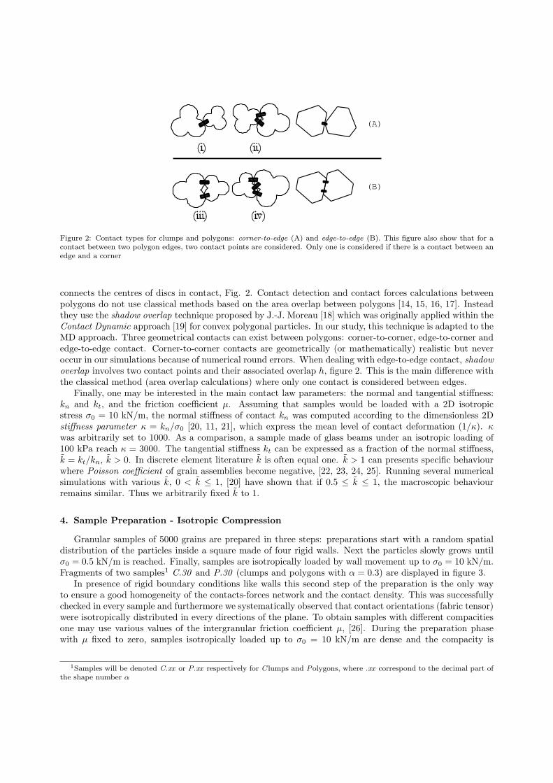
Granular samples of 5000 grains are prepared in three steps: preparations start with a random spatialdistribution of the particles inside a square made of four rigid walls. Next the particles slowly grows untilσ0 = 0.5 kN/m is reached. Finally, samples are isotropically loaded by wall movement up to σ0 = 10 kN/m.Fragments of two samples1 C.30 and P.30 (clumps and polygons with α = 0.3) are displayed in figure 3.

In presence of rigid boundary conditions like walls this second step of the preparation is the only wayto ensure a good homogeneity of the contacts-forces network and the contact density. This was successfullychecked in every sample and furthermore we systematically observed that contact orientations (fabric tensor)were isotropically distributed in every directions of the plane. To obtain samples with different compacitiesone may use various values of the intergranular friction coefficient µ, [26]. During the preparation phasewith µ fixed to zero, samples isotropically loaded up to σ0 = 10 kN/m are dense and the compacity is

1Samples will be denoted C.xx or P.xx respectively for C lumps and Polygons, where .xx correspond to the decimal part ofthe shape number α

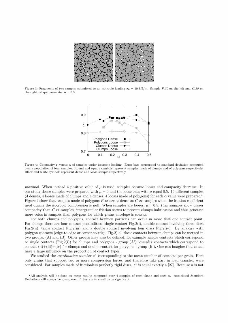
Figure 3: Fragments of two samples submitted to an isotropic loading σ0 = 10 kN/m. Sample P.30 on the left and C.30 onthe right. shape parameter α = 0.3

0.7

0.8

0.9

0 0.1 0.2 0.3 0.4 0.5

Polygons DensePolygons Loose

Clumps DenseClumps Loose

ξ

α

Figure 4: Compacity ξ versus α of samples under isotropic loading. Error bars correspond to standard deviation computedover a population of four samples. Round and square symbols represent samples made of clumps and of polygons respectively.Black and white symbols represent dense and loose sample respectively

maximal. When instead a positive value of µ is used, samples became looser and compacity decrease. Inour study dense samples were prepared with µ = 0 and the loose ones with µ equal 0.5. 16 different samples(4 denses, 4 looses made of clumps and 4 denses, 4 looses made of polygons) for each α value were prepared2.Figure 4 show that samples made of polygons P.xx are as dense as C.xx samples when the friction coefficientused during the isotropic compression is null. When samples are looser, µ = 0.5, P.xx samples show biggercompacity than C.xx samples: intergranular friction seems to prevent clumps imbrication and thus generatemore voids in samples than polygons for which grains envelope is convex.

For both clumps and polygons, contact between particles can occur in more that one contact point.For clumps there are four contact possibilities: single contact Fig.2(i), double contact involving three discsFig.2(ii), triple contact Fig.2(iii) and a double contact involving four discs Fig.2(iv). By analogy withpolygon contacts (edge-to-edge or corner-to-edge, Fig.2) all these contacts between clumps can be merged intwo groups, (A) and (B). Other groups may also be defined, for example simple contacts which correspondto single contacts (Fig.2(i)) for clumps and polygons - group (A’); complex contacts which correspond tocontact (ii)+(iii)+(iv) for clumps and double contact for polygons - group (B’). One can imagine that α canhave a large influence on the proportion of contact types.

We studied the coordination number z∗ corresponding to the mean number of contacts per grain. Hereonly grains that support two or more compression forces, and therefore take part in load transfer, wereconsidered. For samples made of frictionless perfectly rigid discs, z∗ is equal exactly 4 [27]. Because κ is not

2All analysis will be done on mean results computed over 4 samples of each shape and each α. Associated StandardDeviations will always be given, even if they are to small to be significant.

(A’)

3

4.5

6

0 0.1 0.2 0.3 0.4 0.5

Polygons DensePolygons Loose

Clumps DenseClumps Loose

z∗

α

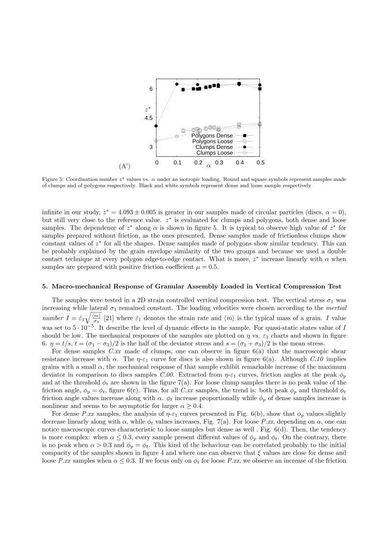
Figure 5: Coordination number z∗ values vs. α under an isotropic loading. Round and square symbols represent samples madeof clumps and of polygons respectively. Black and white symbols represent dense and loose sample respectively

infinite in our study, z∗ = 4.093 ± 0.005 is greater in our samples made of circular particles (discs, α = 0),but still very close to the reference value. z∗ is evaluated for clumps and polygons, both dense and loosesamples. The dependence of z∗ along α is shown in figure 5. It is typical to observe high value of z∗ forsamples prepared without friction, as the ones presented. Dense samples made of frictionless clumps showconstant values of z∗ for all the shapes. Dense samples made of polygons show similar tendency. This canbe probably explained by the grain envelope similarity of the two groups and because we used a doublecontact technique at every polygon edge-to-edge contact. What is more, z∗ increase linearly with α whensamples are prepared with positive friction coefficient µ = 0.5.

5. Macro-mechanical Response of Granular Assembly Loaded in Vertical Compression Test

The samples were tested in a 2D strain controlled vertical compression test. The vertical stress σ1 wasincreasing while lateral σ3 remained constant. The loading velocities were chosen according to the inertial

number I = ε1

√

〈m〉σ3

[21] where ε1 denotes the strain rate and 〈m〉 is the typical mass of a grain. I value

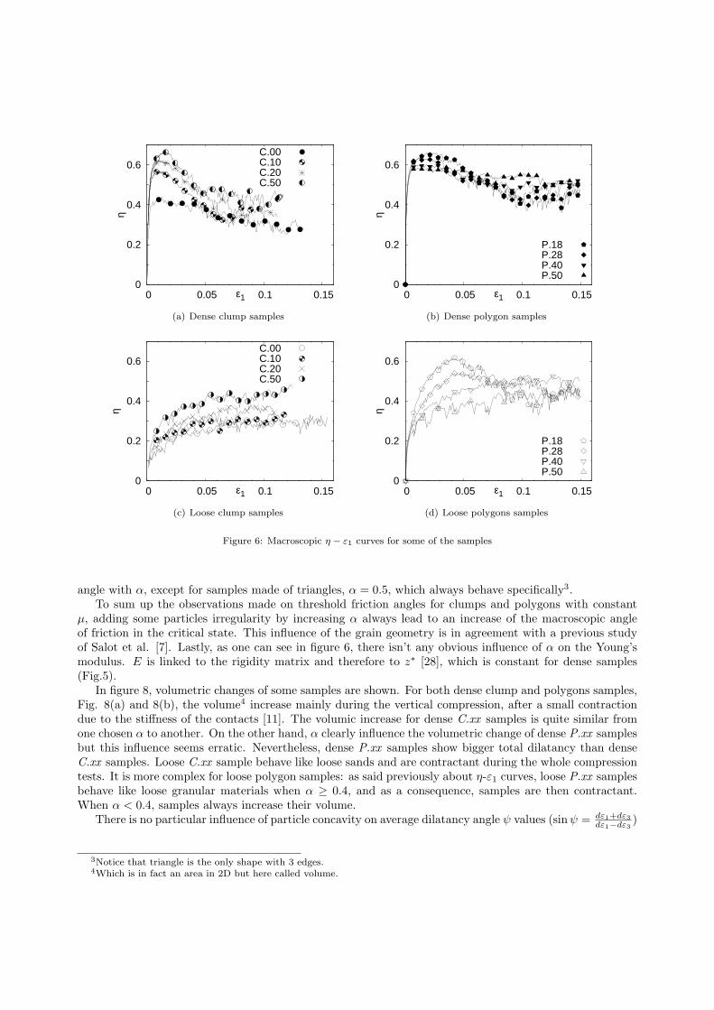
was set to 5 · 10−5. It describe the level of dynamic effects in the sample. For quasi-static states value of Ishould be low. The mechanical responses of the samples are plotted on η vs. ε1 charts and shown in figure6. η = t/s, t = (σ1 − σ3)/2 is the half of the deviator stress and s = (σ1 + σ3)/2 is the mean stress.

For dense samples C.xx made of clumps, one can observe in figure 6(a) that the macroscopic shearresistance increase with α. The η-ε1 curve for discs is also shown in figure 6(a). Although C.10 impliesgrains with a small α, the mechanical response of that sample exhibit remarkable increase of the maximumdeviator in comparison to discs samples C.00. Extracted from η-ε1 curves, friction angles at the peak φp

and at the threshold φt are shown in the figure 7(a). For loose clump samples there is no peak value of thefriction angle, φp = φt, figure 6(c). Thus, for all C.xx samples, the trend is: both peak φp and threshold φt

friction angle values increase along with α. φt increase proportionally while φp of dense samples increase isnonlinear and seems to be asymptotic for larger α ≥ 0.4.

For dense P.xx samples, the analysis of η-ε1 curves presented in Fig. 6(b), show that φp values slightlydecrease linearly along with α, while φt values increases, Fig. 7(a). For loose P.xx, depending on α, one cannotice macroscopic curves characteristic to loose samples but dense as well , Fig. 6(d). Then, the tendencyis more complex: when α ≤ 0.3, every sample present different values of φp and φt. On the contrary, thereis no peak when α > 0.3 and φp = φt. This kind of the behaviour can be correlated probably to the initialcompacity of the samples shown in figure 4 and where one can observe that ξ values are close for dense andloose P.xx samples when α ≤ 0.3. If we focus only on φt for loose P.xx, we observe an increase of the friction

0

0.2

0.4

0.6

0 0.05 0.1 0.15

η

ε1

C.00C.10C.20C.50

(a) Dense clump samples

0

0.2

0.4

0.6

0 0.05 0.1 0.15

η

ε1

P.18P.28P.40P.50

(b) Dense polygon samples

0

0.2

0.4

0.6

0 0.05 0.1 0.15

η

ε1

C.00C.10C.20C.50

(c) Loose clump samples

0

0.2

0.4

0.6

0 0.05 0.1 0.15

η

ε1

P.18P.28P.40P.50

(d) Loose polygons samples

Figure 6: Macroscopic η − ε1 curves for some of the samples

angle with α, except for samples made of triangles, α = 0.5, which always behave specifically3.To sum up the observations made on threshold friction angles for clumps and polygons with constant

µ, adding some particles irregularity by increasing α always lead to an increase of the macroscopic angleof friction in the critical state. This influence of the grain geometry is in agreement with a previous studyof Salot et al. [7]. Lastly, as one can see in figure 6, there isn’t any obvious influence of α on the Young’smodulus. E is linked to the rigidity matrix and therefore to z∗ [28], which is constant for dense samples(Fig.5).

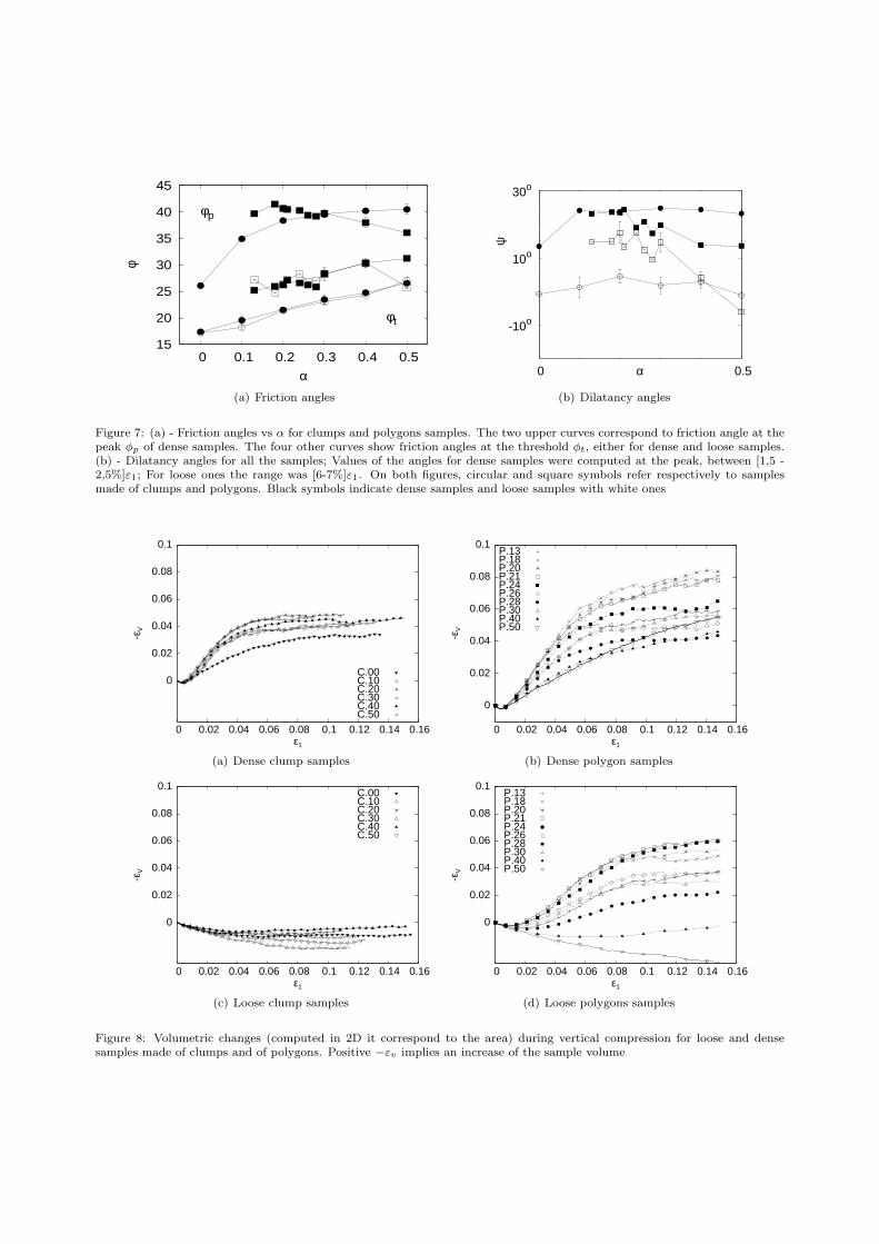
In figure 8, volumetric changes of some samples are shown. For both dense clump and polygons samples,Fig. 8(a) and 8(b), the volume4 increase mainly during the vertical compression, after a small contractiondue to the stiffness of the contacts [11]. The volumic increase for dense C.xx samples is quite similar fromone chosen α to another. On the other hand, α clearly influence the volumetric change of dense P.xx samplesbut this influence seems erratic. Nevertheless, dense P.xx samples show bigger total dilatancy than denseC.xx samples. Loose C.xx sample behave like loose sands and are contractant during the whole compressiontests. It is more complex for loose polygon samples: as said previously about η-ε1 curves, loose P.xx samplesbehave like loose granular materials when α ≥ 0.4, and as a consequence, samples are then contractant.When α < 0.4, samples always increase their volume.

There is no particular influence of particle concavity on average dilatancy angle ψ values (sinψ = dε1+dε3

dε1−dε3

)

3Notice that triangle is the only shape with 3 edges.4Which is in fact an area in 2D but here called volume.

15

20

25

30

35

40

45

0 0.1 0.2 0.3 0.4 0.5

φ

α

φp

φt

(a) Friction angles

-10o

10o

30o

0 0.5

ψ

α

(b) Dilatancy angles

Figure 7: (a) - Friction angles vs α for clumps and polygons samples. The two upper curves correspond to friction angle at thepeak φp of dense samples. The four other curves show friction angles at the threshold φt, either for dense and loose samples.(b) - Dilatancy angles for all the samples; Values of the angles for dense samples were computed at the peak, between [1,5 -2,5%]ε1; For loose ones the range was [6-7%]ε1. On both figures, circular and square symbols refer respectively to samplesmade of clumps and polygons. Black symbols indicate dense samples and loose samples with white ones

0

0.02

0.04

0.06

0.08

0.1

0 0.02 0.04 0.06 0.08 0.1 0.12 0.14 0.16

-εV

ε1

C.00C.10C.20C.30C.40C.50

(a) Dense clump samples

0

0.02

0.04

0.06

0.08

0.1

0 0.02 0.04 0.06 0.08 0.1 0.12 0.14 0.16

-εV

ε1

P.13P.18P.20P.21P.24P.26P.28P.30P.40P.50

(b) Dense polygon samples

0

0.02

0.04

0.06

0.08

0.1

0 0.02 0.04 0.06 0.08 0.1 0.12 0.14 0.16

-εV

ε1

C.00C.10C.20C.30C.40C.50

(c) Loose clump samples

0

0.02

0.04

0.06

0.08

0.1

0 0.02 0.04 0.06 0.08 0.1 0.12 0.14 0.16

-εV

ε1

P.13P.18P.20P.21P.24P.26P.28P.30P.40P.50

(d) Loose polygons samples

Figure 8: Volumetric changes (computed in 2D it correspond to the area) during vertical compression for loose and densesamples made of clumps and of polygons. Positive −εv implies an increase of the sample volume

0 %

20 %

40 %

60 %

80 %

100 %

0.1 0.2 0.3 0.4 0.5

α

Polygons DensePolygons Loose

Clumps DenseClumpsLoose

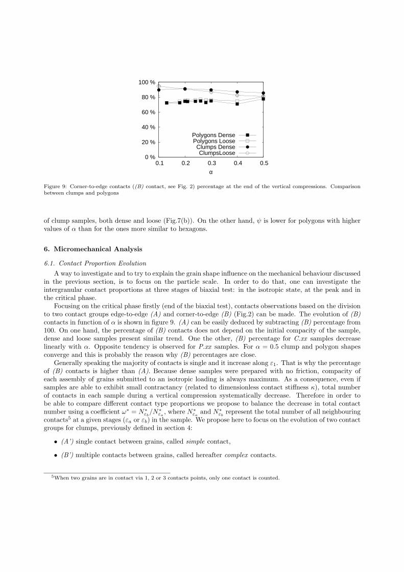
Figure 9: Corner-to-edge contacts ((B) contact, see Fig. 2) percentage at the end of the vertical compressions. Comparisonbetween clumps and polygons

of clump samples, both dense and loose (Fig.7(b)). On the other hand, ψ is lower for polygons with highervalues of α than for the ones more similar to hexagons.

6. Micromechanical Analysis

6.1. Contact Proportion Evolution

A way to investigate and to try to explain the grain shape influence on the mechanical behaviour discussedin the previous section, is to focus on the particle scale. In order to do that, one can investigate theintergranular contact proportions at three stages of biaxial test: in the isotropic state, at the peak and inthe critical phase.

Focusing on the critical phase firstly (end of the biaxial test), contacts observations based on the divisionto two contact groups edge-to-edge (A) and corner-to-edge (B) (Fig.2) can be made. The evolution of (B)contacts in function of α is shown in figure 9. (A) can be easily deduced by subtracting (B) percentage from100. On one hand, the percentage of (B) contacts does not depend on the initial compacity of the sample,dense and loose samples present similar trend. One the other, (B) percentage for C.xx samples decreaselinearly with α. Opposite tendency is observed for P.xx samples. For α = 0.5 clump and polygon shapesconverge and this is probably the reason why (B) percentages are close.

Generally speaking the majority of contacts is single and it increase along ε1. That is why the percentageof (B) contacts is higher than (A). Because dense samples were prepared with no friction, compacity ofeach assembly of grains submitted to an isotropic loading is always maximum. As a consequence, even ifsamples are able to exhibit small contractancy (related to dimensionless contact stiffness κ), total numberof contacts in each sample during a vertical compression systematically decrease. Therefore in order tobe able to compare different contact type proportions we propose to balance the decrease in total contactnumber using a coefficient ω∗ = N∗

εb/N∗

εa, where N∗

εaand N∗

εbrepresent the total number of all neighbouring

contacts5 at a given stages (εa or εb) in the sample. We propose here to focus on the evolution of two contactgroups for clumps, previously defined in section 4:

• (A’) single contact between grains, called simple contact,

• (B’) multiple contacts between grains, called hereafter complex contacts.

5When two grains are in contact via 1, 2 or 3 contacts points, only one contact is counted.

0.2

0.4

0.6

0.8

1

1.2

1.4

1.6

0.1 0.2 0.3 0.4 0.5

λ

α

SingleComplex

(a)

0.2

0.4

0.6

0.8

1

1.2

1.4

1.6

0.1 0.2 0.3 0.4 0.5

λ

α

SingleComplex

(b)

Figure 10: Transformation of complex clump contacts to simple, quantified by λ and evaluated between the maximum stressdeviator (peak) and the isotropic initial state for figure (a), and between the peak and the critical state, Fig. (b)

We observed the evolution of clump contact number of each group between two successive stages andnormalised that evolution with ω∗. Thus we define a new variable λ = ω∗ · Nεa/Nεb , where Nεa andNεb denotes the number of (A’) or (B’) contacts between two different stages εa and εb of the verticalcompression. In figure 10(a), we can observe that for α = 0.1, λ is smaller than 1 for complex (B’) contactsand greater than 1 for simple (A’). These were computed between εa: isotropic state and εb: maximumstress deviator (peak). This can be analysed as a transformation of complex contacts into simple betweenthese two stages. When all complex contacts transform into simple, graphical points are in equal distancefrom 1, 1−λ(B’) = λ(A’) − 1. If 1−λ(B’) > λ(A’) − 1, it means that some complex contacts transform in

simple but some disappear as well. When α goes to 0.5 these transformations are still active but with lessintensity. Geometrical imbrications between clumps increase with α and are ”more difficult to lose” duringbiaxial test. λ seems to reach a threshold when α ≥ 0.4, Fig. 10(a). This last observation may be correlatedto the evolution of φp which also reach a threshold for the same value of α, Fig. 7(a).

Focusing on λ between the peak and the critical state, Fig. 10(b), we can observe that the increase ofsimple contacts is small for every α (λ(A’) − 1 ≃ 0) and complex contact are mainly lost 1 − λ(B’) > 0,

especially when α is small. Greater is α, smaller is the amount of lost complex contacts (grains imbricationare destroyed less). This may explain that φt of clumps increase with α, Fig. 7(a).

6.2. Contact Orientation Evolution

Contact orientations and their evolutions during the vertical compression tests are classically analysed.Usually one can observe that contacts are lost in the extension direction and gained in the direction ofcompression, [29]. In figure 11 we present statistical analysis of contact orientations between different stagesfor two values of α, by evaluation of P (θ) = Nεb

(θ)/Nεa(θ), where εa and εb correspond to two successive

stages, Nεx(θ) is the number of contacts in the direction θ for the stage εx; P (θi) = 1 express that the

number of contact in the direction θi remain constant between the two studied stages; if P (θi) < 1, contactsare lost and if P (θi) > 1 contacts are gained in θi direction. When we focus on the evolution of contactnumbers between the isotropic state and the peak, Fig. 11(a) for α = 0.2 and Fig. 11(c) for α = 0.5, we canobserve that there is no contact gain in any direction. P (θ) ≃ 1 in the compression direction and P (θ) < 1indicate that most of the contacts are lost in the extension direction. Computed of θ, the mean of P issmaller than 1 for both α and we have checked that it is almost constant for all studies α. This simplyindicate that contacts are mainly lost during the vertical compression of dense samples made of clumps.Finally, we noticed that greater α is, bigger is the imbrication between grains and smaller is the amount ofcontacts lost in the extension direction.

(a) α = 0.2

(b) α = 0.2

(c) α = 0.5 (d) α = 0.5

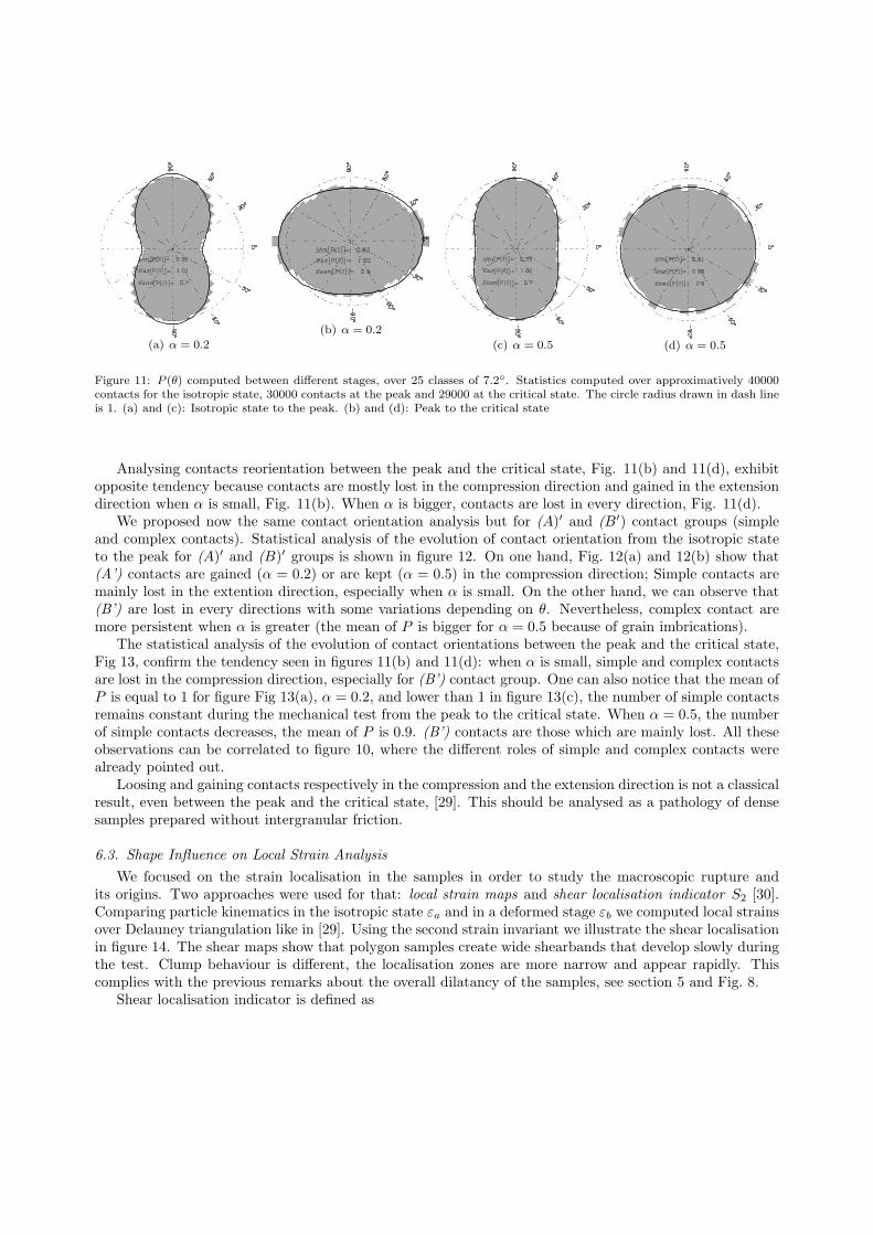
Figure 11: P (θ) computed between different stages, over 25 classes of 7.2◦. Statistics computed over approximatively 40000contacts for the isotropic state, 30000 contacts at the peak and 29000 at the critical state. The circle radius drawn in dash lineis 1. (a) and (c): Isotropic state to the peak. (b) and (d): Peak to the critical state

Analysing contacts reorientation between the peak and the critical state, Fig. 11(b) and 11(d), exhibitopposite tendency because contacts are mostly lost in the compression direction and gained in the extensiondirection when α is small, Fig. 11(b). When α is bigger, contacts are lost in every direction, Fig. 11(d).

We proposed now the same contact orientation analysis but for (A)′ and (B′) contact groups (simpleand complex contacts). Statistical analysis of the evolution of contact orientation from the isotropic stateto the peak for (A)′ and (B)′ groups is shown in figure 12. On one hand, Fig. 12(a) and 12(b) show that(A’) contacts are gained (α = 0.2) or are kept (α = 0.5) in the compression direction; Simple contacts aremainly lost in the extention direction, especially when α is small. On the other hand, we can observe that(B’) are lost in every directions with some variations depending on θ. Nevertheless, complex contact aremore persistent when α is greater (the mean of P is bigger for α = 0.5 because of grain imbrications).

The statistical analysis of the evolution of contact orientations between the peak and the critical state,Fig 13, confirm the tendency seen in figures 11(b) and 11(d): when α is small, simple and complex contactsare lost in the compression direction, especially for (B’) contact group. One can also notice that the mean ofP is equal to 1 for figure Fig 13(a), α = 0.2, and lower than 1 in figure 13(c), the number of simple contactsremains constant during the mechanical test from the peak to the critical state. When α = 0.5, the numberof simple contacts decreases, the mean of P is 0.9. (B’) contacts are those which are mainly lost. All theseobservations can be correlated to figure 10, where the different roles of simple and complex contacts werealready pointed out.

Loosing and gaining contacts respectively in the compression and the extension direction is not a classicalresult, even between the peak and the critical state, [29]. This should be analysed as a pathology of densesamples prepared without intergranular friction.

6.3. Shape Influence on Local Strain Analysis

We focused on the strain localisation in the samples in order to study the macroscopic rupture andits origins. Two approaches were used for that: local strain maps and shear localisation indicator S2 [30].Comparing particle kinematics in the isotropic state εa and in a deformed stage εb we computed local strainsover Delauney triangulation like in [29]. Using the second strain invariant we illustrate the shear localisationin figure 14. The shear maps show that polygon samples create wide shearbands that develop slowly duringthe test. Clump behaviour is different, the localisation zones are more narrow and appear rapidly. Thiscomplies with the previous remarks about the overall dilatancy of the samples, see section 5 and Fig. 8.

Shear localisation indicator is defined as

(a) α = 0.2, (A’) contacts (b) α = 0.5, (A’) contacts (c) α = 0.2, (B’) contacts (d) α = 0.5, (B’) contacts

Figure 12: P (θ) computed between the isotropic state and the peak, over 25 classes of 7.2◦. The circle radius drawn in dashline is 1

(a) α = 0.2, (A’) contacts

(b) α = 0.5, (A’) contacts (c) α = 0.2, (B’) contacts(d) α = 0.5, (B’) contacts

Figure 13: P (θ) computed between the peak and the critical state, over 25 classes of 7.2◦. The circle radius drawn in dash lineis 1

(a) Clumps (b) Polygons

Figure 14: Shearmaps on samples made of grains with α = 0.3. ε1 = 0 − 13.5%

0.2

0.4

0.6

0 0.05 0.1 0.15ε1

Dense Clump α=0.5

Loose Clump α=0.3

Dense Poly α=0.24

Loose Poly α=0.28

Loose Poly α=0.4S2

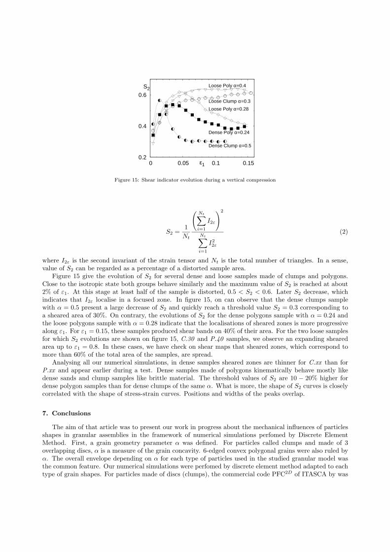
Figure 15: Shear indicator evolution during a vertical compression

S2 =1

Nt

(

Nt∑

i=1

I2ε

)2

Nt∑

i=1

I22ε

(2)

where I2ε is the second invariant of the strain tensor and Nt is the total number of triangles. In a sense,value of S2 can be regarded as a percentage of a distorted sample area.

Figure 15 give the evolution of S2 for several dense and loose samples made of clumps and polygons.Close to the isotropic state both groups behave similarly and the maximum value of S2 is reached at about2% of ε1. At this stage at least half of the sample is distorted, 0.5 < S2 < 0.6. Later S2 decrease, whichindicates that I2ε localise in a focused zone. In figure 15, on can observe that the dense clumps samplewith α = 0.5 present a large decrease of S2 and quickly reach a threshold value S2 = 0.3 corresponding toa sheared area of 30%. On contrary, the evolutions of S2 for the dense polygons sample with α = 0.24 andthe loose polygons sample with α = 0.28 indicate that the localisations of sheared zones is more progressivealong ε1. For ε1 = 0.15, these samples produced shear bands on 40% of their area. For the two loose samplesfor which S2 evolutions are shown on figure 15, C.30 and P.40 samples, we observe an expanding shearedarea up to ε1 = 0.8. In these cases, we have check on shear maps that sheared zones, which correspond tomore than 60% of the total area of the samples, are spread.

Analysing all our numerical simulations, in dense samples sheared zones are thinner for C.xx than forP.xx and appear earlier during a test. Dense samples made of polygons kinematically behave mostly likedense sands and clump samples like brittle material. The threshold values of S2 are 10 − 20% higher fordense polygon samples than for dense clumps of the same α. What is more, the shape of S2 curves is closelycorrelated with the shape of stress-strain curves. Positions and widths of the peaks overlap.

7. Conclusions

The aim of that article was to present our work in progress about the mechanical influences of particlesshapes in granular assemblies in the framework of numerical simulations perfomed by Discrete ElementMethod. First, a grain geometry parameter α was defined. For particles called clumps and made of 3overlapping discs, α is a measure of the grain concavity. 6-edged convex polygonal grains were also ruled byα. The overall envelope depending on α for each type of particles used in the studied granular model wasthe common feature. Our numerical simulations were perfomed by discrete element method adapted to eachtype of grain shapes. For particles made of discs (clumps), the commercial code PFC2D of ITASCA by was

used. For polygonal particles, we developed our own computer code which implement some special contactdetection between objects in the framework of Molecular Dynamic approach. In this paper we highlightedthat changing grain geometry influence granular assembly mechanical behaviour under the classical verticalcompression test, also called biaxial test in 2D. More complex grain shapes allow reaching higher levelsof internal friction angle and large volumetric strains comparing to discs. Some clear differences in thebehaviour of polygons (convex) and clump (non-convex) assemblies were shown. One should notice alsothat the chosen shapes of particles demonstrate similarities as well, caused by the global envelope, thatjustify the comparison. Granular assemblies generation and compaction was presented. By the use of twoextremes values of the intergranular friction angle µ, dense and loose samples were prepared, both for samplesmade of clumps and polygons.

First, focusing on the macroscopic mechanical behaviour of our granular model we show that loose sam-ples composed of polygons with low values of α present behaviour typical to consolided soils where theinitial contractance stage was not only due to contact stiffness but also to large intergranular reorganisa-tions. Apart from that, loose and dense samples of all shapes behave as expected (loose samples only showcontractant behaviour while dense ones mostly exhibit large dilatancy), showing similar behaviour whendiscussing friction residual angle φt or percentage of contacts. All samples show higher values of maximuminternal friction angle φp and φt than samples only made of circular grains (each particle is a disc). Thecorrelations between shape parameter α and friction angles are different for clumps and polygons. On onehand, for dense clump samples, φp increase with α and seems to reach a assymptotic value φp = 40◦. Onthe other hand, φp linearly decrease when α goes from 0.13 to 0.5. On that occasion, the particular case oftriangular shape (α = 0.5) is also discussed briefly. Overall dilatancy of clump samples is bigger than theone of disc assemblies, but spectacularly smaller than dilatancy of polygons.

Secondly, at the granular scale, we proposed to correlate macroscopic observations by the meaning ofcontact evolution analysis which lead us to introduce two groups of contacts between particles: single andmultiple, called simple and complex in that paper. Thus, we observed that complex contacts betweenclumps transform to simple and that this process depends on the size of concavities, i.e. α. We tend tolink it with an increase of shear resistance in the case of dense granular samples made of clumps. Focusingon granular assemblies failures, we study shear bands localisation and tried to characterise it by a scalar.It was observed that reflecting shear band were thinner in dense samples made of clumps than ones madeof polygons, whatever α, highlighting evident geometrical imbrications of clumps that way. In a sense,polygons samples behave more like soil, they slowly create wide shearbands, while clump samples resemblebrittle material more.

Acknowledgments

This work was done as a part of CEGEO research project. The authors would like to express specialthanks to F. Radjai, C. Nouguier for fruitful discussions. The authors are indebt to J.-J. Moreau for hisguidance on algorithm for contact detection between polygon objects.

References

[1] J. Lanier, M. Jean, Experiments and numerical simulations with 2D-disks assembly, Powder technology (special issue onNumerical simulations of discrete particle systems) 109 (1–3) (2000) 206–221.

[2] C. Thornton, J. Lanier, Uniaxial compression of granular media: Numerical simulations and physical experiment, in: R. P.Behringer, J. Jenkins (Eds.), Powders and Grains 97, Balkema, Rotterdam, 1997, pp. 223–226.

[3] M. Oda, K. Iwashita (Eds.), Mechanics of granular materials, an introduction, A.A. Balkema, 1999, iSBN 90-5410-461-9.[4] K. Iwashita, M. Oda, Rotational resistance at contacts in the simulation of shear band development by dem, ASCE Journal

of Engineering Mechanics 124 (1998) 285–292.[5] A. Tordesillas, D. C. Stuart, Incorporating rolling resistance and contact anisotropy in micromechanical models of granular

media, Powder Technology 124 (2002) 106–111.[6] F. Gilabert, J.-N. Roux, A. Castellanos, Computer simulation of model cohesive powders: Influence of assembling proce-

dure and contact laws on low consolidation states, Physical Review E 75 (2007) 011303.[7] C. Salot, P. Gotteland, P. Villard, Influence of relative density on granular materials behavior: Dem simulations of triaxial

tests, Granular Matter - in press.

[8] E. Azema, F. Radjai, R. Peyroux, G. Saussine, Force transmission in a packing of pentagonal particles, Physical ReviewE (Statistical, Nonlinear, and Soft Matter Physics) 76 (1) (2007) 011301.

[9] P. A. Cundall, O. D. L. Strack, A discrete numerical model for granular assemblies, Geotechnique 29 (1) (1979) 47–65.[10] D. Rapaport, The Art of Molecular Dynamics Simulation, Cambridge University Press, 1995, iSBN 0-521-82568-7.[11] J.-N. Roux, G. Combe, On the meaning and microscopic origins of “quasistatic deformation” of granular materials, in:

Proceedings of the EM03 ASCE conference, CD-ROM published by ASCE, Seattle, 2003.[12] M. Allen, D. Tildesley, Computer simulation of liquids, Oxford Science Publications, 1994.[13] S. Luding, Stress distribution in static two-dimensional granular model media in the absence of friction, Phys. Rev. E

55 (4) (1997) 4720–4729.[14] M. Hopkins, On the ridging of intact lead ice, Journal of Geophysical Research 99 (1994) 16351,16360.[15] H.-G. Matuttis, Simulation of the pressure distribution under a two-dimensional heap of polygonal particles, Granular

matter 1 (2) (1998) 83–91.[16] F. Alonso-Marroquin, S. Luding, H. J. Herrmann, I. Vardoulakis, The role of the anisotropy in the elastoplastic response

of a polygonal packing, Physical Review E 71 (2005) 051304.[17] F. Alonso-Marroquin, H. J. Herrmann, Calculation of the incremental stress-strain relation of a polygonal packing, Phys.

Rev. E 66 (2) (2002) 021301. doi:10.1103/PhysRevE.66.021301.[18] J.-J. Moreau, Private communication (2006).[19] G. Saussine, C. Cholet, P.-E. Gautier, F. Dubois, C. Bohatier, J.-J. Moreau, Modelling ballast behaviour under dy-

namic loading. part 1: A 2d polygonal discrete element method approach, Computer Methods in Applied Mechanics andEngineering 195 (2006) 2841–2859.

[20] G. Combe, Origines microscopiques du comportement quasi-statique des materiaux granulaires, Ph.D. thesis, Ecole Na-tionale des Ponts et Chaussees, Champs-sur-Marne, France (2001).

[21] J.-N. Roux, F. Chevoir, Discrete numerical simulation and the mechanical behavior of granular materials, Bulletin desLaboratoires des Ponts et Chaussees 254 (2005) 109–138.

[22] B. Emeriault, B. Cambou, A. Mahboudi, Homogenization for granular materials: non reversible behaviour, Mechanics ofcohesive-frictional materials 1 (1996) 199–218.

[23] B. Cambou, P. Dubujet, F. Emeriault, F. Sidoroff, Homogenization for granular materials, European J. of MechanicsA/Solids 14 (1995) 255–276.

[24] J. Bathurst, L. Rothenburg, Micromechanical aspects of isotropic granular assemblies with linear contact interactions,Journal of Applied Mechanics 55 (1988) 17–23.

[25] J. Bathurst, L. Rothenburg, Note on a random isotropic granular material with negative poisson’s ratio, InternationalJournal Engineering Science 26 (1988) 373–383.

[26] B. Chareyre, P. Villard, Dynamic spar elements and dem in two dimensions for the modeling of soil-inclusion problems,Journal of Engineering Mechanics 131 (2005) 689–698.

[27] I. Agnolin, J.-N. Roux, Internal states of model isotropic granular packings. i. assembling process, geometry, and contactnetworks, Physical Review E (Statistical, Nonlinear, and Soft Matter Physics) 76 (6) (2007) 061302.

[28] I. Agnolin, J.-N. Roux, Internal states of model isotropic granular packings. III. Elastic properties., Physical Review E:Statistical, Nonlinear, and Soft Matter Physics 76 (6) (2007) 061304.

[29] F. Calvetti, G. Combe, J. Lanier, Experimental micromechanical analysis of a 2D granular material: relation betweenstructure evolution and loading path, Mechanics of Cohesive-frictional materials 2 (1997) 121–163.

[30] A. Sornette, P. Davy, D. Sornette, Fault growth in brittle-ductile experiments and the mechanics of continental collisions,Journal of geophysical research 98 (1993) 12111–12140.