inventory control in case of unknown demand and control ... · unknown demand and control...
TRANSCRIPT

Inventory Control in Case ofUnknown Demand and Control
Parameters


Inventory Control in Case ofUnknown Demand and Control
Parameters
Proefschrift
ter verkrijging van de graad van doctor aan deUniversiteit van Tilburg, op gezag van de rectormagnificus, prof.dr. Ph. Eijlander, in het openbaar teverdedigen ten overstaan van een door het college voorpromoties aangewezen commissie in de aula van deUniversiteit op vrijdag 7 mei 2010 om 14.15 uur door
Elleke Janssen
geboren op 2 oktober 1980 te Nijmegen.

Promotor: prof.dr.ir. D. den HertogCopromotor: dr.ir. L.W.G. Strijbosch

Preface
Het voorwoord is zowel in het Nederlands als in het Engels geschreven.Hieronder staat de Engelse versie; de Nederlandse versie kunt u vinden oppagina ix.
The preface is the place to thank all those people that have had a direct, or indirect,
influence on the dissertation you are reading right now. I have chosen to write this
part both in English and in Dutch, mainly because the mother tongue of the majority
of the people mentioned in this preface is Dutch. However, since this dissertation is
written in English, apart from the Dutch preface and summary in Dutch, also an
English version of the preface should be present. This is not a direct translation of
the Dutch one, but it covers the same topics.
Let me start thanking the person without whom this dissertation would never have
appeared in the first place: Dick. When I was finishing my master’s thesis, studying
a topic that has nothing in common with this dissertation, he asked me to become a
PhD-student. During my study Econometrics and OR I have never considered this
career path, since doing purely theoretical research is not something I saw myself
doing for four years. However, at the time I was finishing my master’s thesis, there
was a project at Tilburg University, in collaboration with Involvation, with a very
practical application, namely inventory management. And they were looking for a
PhD-student to join the project. So I started my career in academia. Dick is also
my promotor, but not my daily supervisor; that role is for Leo, my copromotor. He
helped me by brainstorming about the difficult theoretical parts in my dissertation,
by giving me new ideas, but also by letting me follow up on my own ideas. I always
liked going to our meetings, even when I was thinking “I did not get any step further
since the last time, help!”. In most cases our meeting let me see that, although I
did not find the great idea on how to move forward, I at least had investigated, and
rejected, some promising ideas that did not lead to anything. By letting me explain
what I had done and what I had tried to show Leo helped me getting further. Even

vi Preface
when Leo retired, approximately the last half year of writing this dissertation, he
never shied away from reading my texts carefully and in doing so, he improved this
dissertation significantly.
Also the discussions with and remarks of Ruud Brekelmans, Fred Janssen and
Hans Moors have a great influence on the contents of this dissertation. They helped
doing the research on which Chapter 2 (Hans), Chapters 3 and 4 (Ruud), and Chapter
5 (Fred) are based. One of these chapters (Chapter 3) is already published, a second
one is almost published and Chapters 2 and 4 will be submitted in the near future.
The last group of people that has had a direct influence on the appearance of
my dissertation is the committee that has read and, probably even more important,
approved it. The committee consists of John Boylan, Ton de Kok, Fred Janssen,
Ruud Brekelmans, Leo Strijbosch and Dick den Hertog.
Next to the relative small group of people that has had a direct influence, there is
a rather large group that (very) indirectly influenced my dissertation. My colleagues
at the department of Econometrics and Operations Research at Tilburg University
belong to this group. They made sure that I liked going to my work all four years and
that I still do. At almost all my working days I am looking forward to the lunch, not
just because I was having an appetite, but mostly because of the talks on all kinds of
serious and mostly non-serious topics, like the food in the university restaurant, the
sport performances (or failures) of last weekend, television programmes, the political
party one has voted for (or is going to vote for), the mall in Tilburg, the departmental
trips that were going to happen or happened, the television in the Triangel and
thousand-and-one other topics. In random order this involves Peter, Herbert, Henk,
Hans Reijnierse, Jacob, Willem, Bart, Annemiek, Ruud Hendrickx, Gerwald, John,
Gijs, Mark Voorneveld, Marieke, Marloes, Salima, Edwin Lohmann, Edwin van Dam,
Rene, Hein, Ruud Brekelmans, Josine and, recently, Mirjam and Iris. After eating
our lunch there is often some time left to kick back and relax a little more and that
time we enjoy in the Triangel. Besides continuing the talks at lunch, watching sports
(unfortunately, the television is not working anymore) and collecting items one gets
when doing grocery shopping at Appie, we solve puzzles (cryptic crosswords, Mona),
play games (Duck rally, Fluxx) or finding (three)double animals: words consisting of
two (or three) animals, that have a non-animal meaning.
Aside from working on my dissertation and relaxing also some ‘real’ work needed
to be done. I taught several courses (Statistics for HBO-graduates, Mathematics 2,
Quantitative Methods 1, Statistics 1, BEM, Mathematics 1 for Economics, Math-

Preface vii
ematics D) and I would like to thank Marieke, Herbert, Willem, Edwin van Dam,
Gert and Marloes for the nice cooperation during these courses. During the first two
years of working at my dissertation I found out that I like teaching very much and
when I got the opportunity to extend my contract in exchange for extra education
tasks, I took that opportunity. I should thank Marieke, Herbert, Peter and Sprint,
the people (and organization) that made this extension possible.
My officemates at Tilburg University, Marlies, Marloes, Katya, Gijs, Frans, Roy
and Mohammed, always had (and have) time for a chat, a cup of coffee, jokes on radio
Veronica or adventure stories of last weekend in which the police does not always have
a positive role. Luckily they also knew when to let my work. Many thanks to all of
you.
Also outside the university buildings there is time to relax with (part of) my
colleagues during Christmas dinners, mathematics D dinners, departmental trips,
visits to the Efteling, Sinterklaas and mostly the game afternoons and evenings, the
(jigsaw) puzzle evenings and the subdepartmental trips (Ruud Hendrickx, Marieke,
John, Gerwald, Edwin Lohmann, Marloes, Josine, Gijs, Mirjam and Iris).
A special paragraph should be awarded to Marieke, Salima and Marloes. Next
to all the fun things we do, these three girls have been there for me during difficult
(personal) times. And they have given me a push when I needed it.
One of the advantages of working as a PhD-student are the conference visits. I
have met nice people (Ingrid Vliegen and her colleagues of TU Eindhoven, Marco
Bijvank, Rommert Dekker, Ruud Teunter, John Boylan and Aris Syntetos), listened
to interesting presentations (and even more not so interesting presentations. . . ) and
enjoyed visiting new and interesting cities.
Besides all colleagues and (other) people from academia, I also want to thank
everyone outside this world that has supported me. My parents, Wim and Annelies,
have always believed that my talents made me special, they have made me do my
best, but have never pushed me in one direction and let me find out what I liked
doing. Who would have imagined that I would end up in education, just like my
father. . .
Raike and Matthijs, my sister and brother-in-law, and Rob, my brother, might
not have had a big influence, but just knowing that they are there for me, helps me.
When I went to the university, 1012years ago, and I came home for the weekend,
the first thing my brother used to ask me, was “When are you going back?”, but
nowadays we can have good talks. The long telephone calls with my sister help me

viii Preface
keeping a hold on reality, since that could get a little lost in academia.
To my family — my grandmother, my aunts and uncles, my cousins — who still
think of me being a regular student: I have finished and starting a ‘real’ job, although
I still will be working at the university for a couple more years. Their questions about
what I was doing exactly, were often difficult to answer without being (to) technical.
My four-year research resulted in this book (most likely unreadable for those without
a mathematics background) and my doctor’s title (if everything goes like planned at
May, 7th).
Also Ab and Ada, my parents-in-law and Frank, Jozien and Lars, my brother-in-
law, sister-in-law and nephew, have always supported me by being there for Mark
and me. We have had many nice conversations, cosy diners, some nice holidays and
celebrated Sinterklaas and Christmas together. They helped my, together with my
family, to keep in touch with reality and made sure that I did not start thinking too
much of myself just because I am able to learn a little easier than the average person.
The birth of nephew opened up a new world for me and showed me how miraculously
fast a human being can develop and grow.
Last, but certainly not least, I must thank Mark, who is already almost nine years
my boyfriend, my friend and my love. He is there for me when I need him. Sometimes
just by putting his arm around me, by offering me a shoulder to cry on or by lending
me his ear; often by enjoying nature together, by planning to travel and making these
plans come true, by having nice and beautiful holidays or just by eating together.

Voorwoord
The preface is available both in English and in Dutch. This is the Dutchversion; you can find the English version at page v.
Het voorwoord is de plek waar menigeen bedankt wordt voor de direct of indirecte
invloed op het tot stand komen van het proefschrift dat nu voor u ligt. Ik heb ervoor
gekozen om dit stukje van mijn proefschrift zowel in het Nederlands als in het Engels
te schrijven, omdat Nederlands de moedertaal is voor verreweg de meeste mensen die
een plekje hebben weten te veroveren in dit voorwoord. Aangezien de rest van het
proefschrift, op de samenvatting na, in het Engels is, is het voorwoord ook in het
Engels beschikbaar en alhoewel het geen letterlijke vertaling is, staat er wel hetzelfde
in.
Laat ik beginnen met degene te bedanken zonder wie dit proefschrift uberhaupt
nooit geschreven zou zijn: Dick. Toen ik bezig was met het onderzoek dat zou leiden
tot mijn afstudeerscriptie, over een onderwerp dat overigens totaal niets met mijn
proefschrift te maken heeft, heeft Dick mij gevraagd om AiO te worden. Ik heb
tijdens mijn studie altijd gezegd dat dat niets voor mij was, dat continu bezig zijn
met (theoretisch) onderzoek. Nu was er op dat moment een project met praktische
toepassing, namelijk voorraadbeheer, in samenwerking met Involvation. En bij dat
project was plek voor een AiO, waarbij Dick aan mij dacht. Zo ben ik dus mijn AiO-
schap ingerold. Dick is ook mijn promotor, maar de ‘dagelijkse’ begeleiding lag meer
bij mijn copromotor, Leo. Hij heeft me geholpen door mee te denken over moeilijke
stukken in mijn onderzoek, nieuwe ideeen aan te dragen, maar mij ook mijn eigen
dingen te laten doen. Onze afspraken waren nooit iets om tegen op te zien, alhoewel
ik wel eens dacht “Ik ben geen *** opgeschoten, wat nu?”. Maar dan bleek tijdens
onze afspraken dat ik stiekem toch wel iets verder gekomen was, doordat ik uit moest
leggen wat me allemaal niet gelukt was. Zelfs toen Leo al met pensioen was, ongeveer
het laatste halve jaar, heeft hij de tijd genomen om alle teksten secuur te blijven lezen
en daardoor nog een flink aantal verbeteringen aangebracht.

x Voorwoord
Naast Leo heb ik inhoudelijk ook veel gehad aan de opmerkingen van en discussies
met Ruud Brekelmans, Fred Janssen en Hans Moors. Ze hebben samen met Leo en
mij het onderzoek gedaan waarop hoofdstuk 2 (Hans), hoofdstukken 3 en 4 (Ruud)
en hoofdstuk 5 (Fred) gebaseerd zijn. Ze zullen dus ook co-auteur zijn van de papers
die nog gaan komen, of die al (bijna) gepubliceerd zijn.
Wat betreft de directe bijdrage aan mijn proefschrift behoort nog een groep
mensen bedankt te worden: de commissie die dit proefschrift gelezen heeft en, mis-
schien wel belangrijker, het goedgekeurd heeft. Dit zijn John Boylan, Ton de Kok,
Fred Janssen, Ruud Brekelmans, Leo Strijbosch en Dick den Hertog.
Naast de relatief kleine groep die direct invloed heeft gehad op dit proefschrift is
er een grote groep die een (zeer) indirecte invloed heeft uitgeoefend. Hiertoe behoren
mijn collega’s die ervoor gezorgd hebben dat ik het al die jaren bij het departement
Econometrie & Operations Research naar mijn zin heb gehad (en nog steeds heb).
Zo goed als iedere dag dat ik gewerkt heb, heb ik uitgekeken naar de lunch. En niet
zozeer omdat ik trek had of zo, maar vanwege de gezellige en vaak ook onzinnige
gesprekken aan tafel over het eten in de mensa, de verscheidene sportprestaties (of
wanprestaties) van het afgelopen weekend, boer zoekt vrouw, daten in het donker en
andere televisieprogramma’s, de politieke partij waarop je gaat stemmen (of gestemd
had), de Tilburgse mall, de departementsuitjes die eraan kwamen of geweest waren,
de televisie in de Triangel en nog duizend-en-een andere onderwerpen. In willekeurige
volgorde gaat het hierbij om Peter, Herbert, Henk, Hans Reijnierse, Jacob, Willem,
Bart, Annemiek, Ruud Hendrickx, Gerwald, John, Gijs, Mark Voorneveld, Marieke,
Marloes, Salima, Edwin Lohmann, Edwin van Dam, Rene, Hein, Ruud Brekelmans,
Josine en sinds kort ook Mirjam en Iris. Na de lunch is het tijd voor nog iets meer
ontspanning om over de after-lunch-dip heen te komen en daarvoor is de Triangel
uitermate geschikt gebleken. Naast een vervolg op de gesprekken aan de lunchtafel,
het volgen van een of andere wedstrijd of het sparen van producten die bij de Appie
te krijgen zijn, is hier altijd ruimte voor een puzzeltje (cryptogrammen, Mona), een
spelletje (eendenrally, Fluxx) of het vinden van (drie)dubbeldieren, zoals zebrapad,
vlinderdas en kadodoos.
Uiteraard moet er ook nog eens af en toe gewerkt worden en naast het onderzoek
voor en schrijven aan mijn proefschrift heb ik behoorlijk wat onderwijs gegeven.
Daarin heb ik zeer prettig samengewerkt met Marieke, Herbert, Willem, Edwin van
Dam, Gert en Marloes. Ik kwam er in mijn eerste twee jaar achter dat ik onderwijs
eigenlijk erg leuk vind en toen ik de kans kreeg om mijn contract met een jaartje te

Voorwoord xi
verlengen in ruil voor extra onderwijs, heb ik die kans met beide handen aangegrepen,
met dank aan Marieke, Herbert, Peter en Sprint, die dat mogelijk gemaakt hebben.
Bij mijn kamergenoten op de UvT, Marlies, Marloes, Katya, Gijs, Frans, Roy en
Mohammed, was (en is) er altijd tijd voor een praatje, een kop koffie, moppen op
radio Veronica of een verhaal over het afgelopen weekend, waar dan de politie een
niet altijd positieve hoofdrol heeft. Gelukkig wisten ze ook wanneer ze me aan het
werk moesten laten gaan. Veel dank daarvoor.
Ook naast het werk op de UvT is er de nodige tijd om te ontspannen met (een
deel van) mijn collega’s tijdens kerstdiners, wiskunde D etentjes, departementsuit-
jes, bezoek aan de Efteling, Sinterklaasvieringen en met name de spelletjesavonden,
de puzzelavonden en de subdepartementale uitjes (Ruud Hendrickx, Marieke, John,
Gerwald, Edwin Lohmann, Marloes, Gijs, Josine, Mirjam, Iris).
Een speciale alinea moet besteed worden aan Marieke, Salima en Marloes, die er
altijd voor me zijn geweest om me door moeilijke (prive-)momenten heen te helpen,
naar me te luisteren, een arm om me heen te slaan en me dat zetje te geven dat ik
nodig had. En dat naast alle leuke dingen die we samen doen en gedaan hebben.
Een van de voordelen van het werken als AiO zijn de (betaalde) congresbezoeken.
Ik heb daarbij leuke mensen ontmoet (met name, maar niet enkel, Ingrid Vliegen
en haar collega’s van de TU Eindhoven, Marco Bijvank, Rommert Dekker, Ruud
Teunter, John Boylan en Aris Syntetos), interessante praatjes aangehoord (en nog
meer minder interessante praatjes. . . ) en interessante steden bezocht.
Naast alle collega’s en (andere) academici, zijn er nog meer mensen die me vooral
moreel gesteund hebben. Mijn ouders, Wim en Annelies, die altijd geloofd hebben dat
mijn talenten mij bijzonder maken en me altijd gesteund hebben om zover mogelijk
te komen, maar me nooit in een richting gestuurd hebben en me zelf hebben laten
uitzoeken wat ik wilde. Dat ik, net als mijn vader, uiteindelijk in het onderwijs
terecht zou komen, zou ik tot een paar jaar geleden niet bedacht hebben. . .
Raike en Matthijs, mijn zusje en mijn zwager, en Rob, mijn broertje, hebben
misschien inhoudelijk niet veel bijgedragen, maar het feit dat ze er zijn als het nodig
is, is voor mij genoeg. Toen ik ging studeren, tien-en-een-half jaar geleden, en ik in
het weekend thuis kwam, was het eerste dat mijn broertje tegen me zei: “Wanneer
ga je weer?”, maar tegenwoordig kunnen we goede gesprekken hebben. De lange
telefoongesprekken met mijn zusje zijn altijd goed om me weer met beide benen in
de werkelijkheid te zetten.
Aan de rest van mijn familie — mijn oma, ooms, tantes, neven, nichten, en

xii Voorwoord
achterneefjes en -nichtjes — voor wie ik toch een beetje de eeuwige student ben: ik
ben nu klaar en ga ‘echt’ werken, al blijf ik nog wel een tijdje op de universiteit
hangen. Hun vragen over wat ik nu precies aan het doen was, waren vaak moeilijk
te beantwoorden zonder al te veel in technische details te duiken en toch te laten
blijken dat het niet zo eenvoudig was als dat ik meestal vertelde. Mijn onderzoek,
dat vier jaar geduurd heeft, heeft uiteindelijk geleid tot dit, voor niet-wiskundigen
waarschijnlijk onleesbare, boekje en tot de titel van ‘doctor’ (als alles goed gaat op 7
mei 2010).
Ook mijn schoonouders, Ab en Ada, mijn zwager en schoonzus, Frank en Jozien,
en mijn neefje Lars, hebben me altijd gesteund door er voor mij en Mark te zijn. We
hebben vele fijne gesprekken gehad, vaak gezellig gegeten, soms samen op vakantie
geweest en Sinterklaas en Kerst samen gevierd. Samen met mijn eigen familie, zorgen
zij ervoor dat ik het nooit te hoog in mijn bol heb gekregen doordat ik toevallig wat
beter dan gemiddeld kan leren. Mijn neefje heeft een hele nieuwe wereld voor mij
geopend en laat zien hoe wonderbaarlijk snel een mens(je) kan groeien, zowel figuurlijk
als letterlijk.
Last, but certainly not least, moet ik Mark bedanken, die al bijna negen jaar
mijn vriend, maatje en liefste is. Hij is er altijd als ik hem nodig heb. Soms door
een arm om me heen te slaan, door een schouder te bieden om op uit te huilen of een
luisterend oor te geven; vaak door samen te genieten van de natuur, samen (plannen
te maken om) te reizen, mooie vakanties te hebben of gewoon samen te eten.

Contents
Preface (voorwoord in Engels) v
Voorwoord (preface in Dutch) ix
1 Introduction 1
1.1 Background . . . . . . . . . . . . . . . . . . . . . . . . . . . . . . . . 1
1.2 Notation . . . . . . . . . . . . . . . . . . . . . . . . . . . . . . . . . . 4
1.3 Introduction to the (R, S) policy and service levels . . . . . . . . . . 5
1.3.1 Inventory control policy . . . . . . . . . . . . . . . . . . . . . 5
1.3.2 Service level . . . . . . . . . . . . . . . . . . . . . . . . . . . . 8
1.4 Contributions and overview . . . . . . . . . . . . . . . . . . . . . . . 12
I Modified distributions 15
2 Modified shifted gamma distributions 17
2.1 Introduction . . . . . . . . . . . . . . . . . . . . . . . . . . . . . . . . 17
2.2 Modified normal distribution . . . . . . . . . . . . . . . . . . . . . . . 19
2.3 Modified shifted gamma distributions . . . . . . . . . . . . . . . . . . 22
2.3.1 Modified gamma distribution with point mass at zero . . . . . 24
2.3.2 Modified gamma distribution truncated at zero . . . . . . . . 26
2.4 Determination of order-up-to levels . . . . . . . . . . . . . . . . . . . 27
2.4.1 Using F+ρ,θ,∆ . . . . . . . . . . . . . . . . . . . . . . . . . . . . 28
2.4.2 Using F ∗ρ,θ,∆ . . . . . . . . . . . . . . . . . . . . . . . . . . . . 29
2.4.3 Results with general distributions . . . . . . . . . . . . . . . . 30
2.5 Mistakenly using the (shifted) gamma distribution . . . . . . . . . . 33
2.5.1 Not using F+ρ,θ,∆ . . . . . . . . . . . . . . . . . . . . . . . . . . 34
2.5.2 Not using F ∗ρ,θ,∆ . . . . . . . . . . . . . . . . . . . . . . . . . . 38

xiv Contents
2.6 Summary results . . . . . . . . . . . . . . . . . . . . . . . . . . . . . 41
II Unknown demand parameters 43
3 Normal demand with unknown demand parameters 45
3.1 Introduction . . . . . . . . . . . . . . . . . . . . . . . . . . . . . . . . 45
3.2 P1 service level criterion . . . . . . . . . . . . . . . . . . . . . . . . . 47
3.3 P2 service level criterion . . . . . . . . . . . . . . . . . . . . . . . . . 49
3.3.1 Only expected demand unknown . . . . . . . . . . . . . . . . 50
3.3.2 Expected demand and its variance unknown (ν known) . . . . 53
3.3.3 Expected demand and its variance unknown (ν unknown) . . 56
3.3.4 Correction of the order-up-to level . . . . . . . . . . . . . . . 58
3.4 Summary results . . . . . . . . . . . . . . . . . . . . . . . . . . . . . 64
4 Gamma demand with unknown demand parameters 67
4.1 Introduction . . . . . . . . . . . . . . . . . . . . . . . . . . . . . . . 67
4.2 P1 service level criterion . . . . . . . . . . . . . . . . . . . . . . . . . 70
4.2.1 Using estimates in determining the order-up-to level . . . . . 70
4.2.2 Determining the correction . . . . . . . . . . . . . . . . . . . 80
4.3 P2 service level criterion . . . . . . . . . . . . . . . . . . . . . . . . . 84
4.3.1 Using estimates in determining the order-up-to level . . . . . . 85
4.3.2 Determining the correction . . . . . . . . . . . . . . . . . . . 91
4.4 Case study . . . . . . . . . . . . . . . . . . . . . . . . . . . . . . . . . 94
4.5 Summary results . . . . . . . . . . . . . . . . . . . . . . . . . . . . . 101
5 Mixed Erlang demand and random inventory control parameters 103
5.1 Introduction . . . . . . . . . . . . . . . . . . . . . . . . . . . . . . . 103
5.2 Demand distribution and inventory policy . . . . . . . . . . . . . . . 105
5.2.1 Inventory policy . . . . . . . . . . . . . . . . . . . . . . . . . . 105
5.2.2 Demand distribution . . . . . . . . . . . . . . . . . . . . . . . 106
5.2.3 Determining the order-up-to level . . . . . . . . . . . . . . . . 108
5.3 Validations and results . . . . . . . . . . . . . . . . . . . . . . . . . . 109
5.4 Summary results . . . . . . . . . . . . . . . . . . . . . . . . . . . . . 113

Contents xv
6 Conclusions and future research 115
6.1 Conclusions . . . . . . . . . . . . . . . . . . . . . . . . . . . . . . . . 115
6.2 Ideas for future research . . . . . . . . . . . . . . . . . . . . . . . . . 118
A Derivations Chapter 2 123
A.1 Derivation of equations (2.1) and (2.2) . . . . . . . . . . . . . . . . . 123
A.2 First three moments of shifted gamma distribution . . . . . . . . . . 124
B Nested linear regression 129
C Derivations Chapter 3 137
C.1 Independence of achieved performance of µ and σ . . . . . . . . . . . 137
C.1.1 S(dt, stτ, cτβ) . . . . . . . . . . . . . . . . . . . . . . . . . . . . 137
C.1.2 S(dt, stτ, cτβ) . . . . . . . . . . . . . . . . . . . . . . . . . . . . 138
C.1.3 S(dt + κi (νt, t, β) st, stτ, cτβ) . . . . . . . . . . . . . . . . . . . 139
D Derivations Chapter 4 141
D.1 The attained service level in simulation . . . . . . . . . . . . . . . . 141
D.2 Equality order-up-to levels under P1 and P2 if demand is exponential 141
D.3 Simulation results . . . . . . . . . . . . . . . . . . . . . . . . . . . . . 142
E Derivations Chapter 5 157
E.1 Fitting a mixed-Erlang distribution . . . . . . . . . . . . . . . . . . . 157
E.2 Expected backlog at start replenishment cycle . . . . . . . . . . . . . 158
E.3 Distribution of demand during lead time and review period . . . . . . 161
E.4 Expected backlog at end replenishment cycle . . . . . . . . . . . . . . 164
Bibliography 167
Nederlandse samenvatting (summary in Dutch) 173
Author index 181
Subject index 183


Chapter 1
Introduction
This chapter starts with a background literature review. The next sectioncontains notation that is used throughout this dissertation. Section 1.3introduces inventory control as it is used in this research. The last sectionprovides an overview of this dissertation.
1.1 Background
Inventory control involves decisions on what to order, when, and in what quantity.
Standard text books on inventory management (see e.g., Silver et al., 1998, or Zipkin,
2000) provide methods to deal with these decisions. These methods need information
about the (distribution of) demand during some period, e.g., the demand during lead
time or during the review period. Bulinskaya (1990) discriminates between three
situations:
(a) the type of distribution is known, but its parameters are unspecified;
(b) only several first moments of the demand distribution are known;
(c) there is no prior knowledge about the demand.
The third situation is of course the most realistic and different approaches to deal with
situation (c) have been proposed in literature. These approaches can be categorized
into parametric and nonparametric methods. An example of a parametric method is
using Bayesian models; examples of the nonparametric methods include using order
statistics, the bootstrap procedure and kernel densities.
One of the most widespread approaches to deal with unknown demand is assuming
a distribution, estimating its parameters and replacing the unknown parameters by its

2 Chapter 1. Introduction
estimates in the theoretically correct formulae in which distribution and parameters
are supposed to be known. Sani and Kingsman (1997), Artto and Pylkkanen (1999),
Strijbosch et al. (2000) and Syntetos and Boylan (2006) use this approach with dif-
ferent inventory models, while Kottas and Lau (1980) provide a short discussion on
estimating the parameters needed for their model. Another parametric method is the
Bayesian approach; Azoury and Miller (1984), Azoury (1985) and Karmarkar (1994)
are three examples of this approach. Also Larson et al. (2001) use it, but they intro-
duce a nonparametric form. Other nonparametric approaches involve order statistics,
references include Lordahl and Bookbinder (1994) and Liyanage and Shanthikumar
(2005), the bootstrap procedure, see, e.g., Bookbinder and Lordahl (1989) and Fricker
and Goodhart (2000), or using kernel densities, see Strijbosch and Heuts (1992).
This dissertation is mainly about the effect of forecasting on inventory control.
Most of the literature is either on forecasting or on inventory control, but one can
easily imagine that forecasting influences inventory control. Although not many pa-
pers consider both forecasting and inventory control, the problem has already been
mentioned in 1958 (Scarf, 1958). He considers situation (b): it is assumed that the
mean and variance of demand are known and considers a set of two-point distribu-
tions to solve a max-min objective function (maximize the minimal profit). Hayes
(1969) considers situation (a) with two different demand distributions. More recent
references include Watson (1987), Strijbosch and Heuts (1992), Snyder et al. (2002),
Bertsimas and Thiele (2006), Lu et al. (2006) and Syntetos and Boylan (2006). Wat-
son (1987) considers Erlang distributed demand and studies the effect forecasting has
on the attained service using simulation. Strijbosch and Heuts (1992) use simulation
to show the trade-off between attained service and expected average costs while es-
timating the lead time demand in four different ways, including a distribution-free
approach. Snyder et al. (2002) use simulation to show the effects of using adapted
exponentially smoothed forecasts, which incorporates the possibility of having non-
constant variance. Bertsimas and Thiele (2006) assume that the mean and variance
of the demand are known, while the family to which it belongs, is not and use ro-
bust optimization to find good inventory control parameters. Lu et al. (2006) focus
on the way the demand forecasts evolve over time as more information becomes
available and use that to find solution bounds and cost error bounds for general dy-
namic inventory models with possibly nonstationary and autocorrelated demands.
Syntetos and Boylan (2006) compare four estimators for intermittent demand and
study their stock control performance using an empirical data sample containing
1.1. Background 3
monthly demand of 3000 stock keeping units during a period of two years.
Part II of this dissertation deals with the effect of estimating unspecified param-
eters. Therefore, it deals with situation (a), not (c): the true distribution is known,
but its parameters are unspecified. Silver and Rahnama (1986, 1987) investigate the
effect of estimating parameters in a reorder point, order quantity inventory policy
(known as an (s,Q) or (r, Q) policy in literature) with a cost criterion. They construct
a function that determines the expected cost of estimating the demand distribution
rather than knowing it and they conclude that this function is not symmetrical:
underestimating causes larger costs than overestimating. In the second article they
propose a method that deliberately biases the reorder point upwards. Strijbosch et al.
(1997) and Strijbosch and Moors (2005) investigate the same effect for a periodic re-
view, order-up-to level inventory policy with a service level criterion under normally
distributed demand. Both papers conclude that also in this case the order-up-to level
needs to be biased upwards. Note that the reorder point, order quantity and periodic
review, order-up-to level policies are equivalent (see Silver et al., 1998), so the results
of Silver and Rahnama (1986, 1987) apply for the periodic review, order-up-to level
policy and the results of Strijbosch et al. (1997) and Strijbosch and Moors (2005) for
the reorder point, order quantity policy as well.
Both in practice and in literature demand is often assumed to be normally dis-
tributed, see Zeng and Hayya (1999). However, the normal distribution can take on
negative values, while in practice demand cannot be negative (unless one considers
net demand: demanded goods minus returned goods). Strijbosch and Moors (2006)
develop two modified normal distributions to tackle this problem: one is truncated at
zero; the other assigns a value of zero to all negative values, creating a point mass at
zero. They derive the new order-up-to levels and show comparisons between results
using the new demand distributions and mistakenly using a (nonmodified) normal
distribution. One could see this as a particular case of situation (b), as the wrong
distribution is assumed, while the mean and variance of the demand are known.
In Part I of the dissertation these modified demand distributions are discussed
further and two new demand distributions are introduced. A gamma distribution
does not have negative values, but one can shift such a distribution to the left, and
then negative values will occur. Starting from this shifted gamma distribution we
develop two modified shifted gamma distributions.
4 Chapter 1. Introduction
1.2 Notation
This section contains the notation as it is used throughout this dissertation. If in the
chapter itself some specific notation is used, it is explained in that chapter.
Dℓ : demand during ℓ units of time
D : demand during 1 unit of time
R : length of the review period
L : length of the lead time
S : order-up-to level
α : P1 service level; cycle service
β : P2 service level; fill rate
P (A) : probability of event A
E [X ] , µX : expected value of X
V [X ] , σ2X : variance of X
SD [X ] , σX : standard deviation of X (SD [X ] =√
V [X ])
CX , νX : coefficient of variation of X (CX = νX = σX/µX)
(x)+ : maximum of 0 and x ((x)+ = max{x, 0})IC : indicator function: 1 if C is true and 0 otherwise
pdf : shorthand notation for probability density function
cdf : shorthand notation for cumulative distribution function
f(x) : a (general) probability density function (pdf)
F (x) : a (general) cumulative distribution function (cdf)
fparameters(x) : a pdf with its distribution parameters
Fparameters(x) : a cdf with its distribution parameters
ϕ(x) : the pdf of a standard normally distributed variate
Φ(x) : the cdf of a standard normally distributed variate
The length of the review period, length of the lead time and the order-up-to level
are denoted with capital letters; this usually implies that these variables are random
variables. However, it depends on the chapter whether these are random or not. The
order-up-to level is assumed to be random in Part II; the length of the review period
and lead time are only assumed to be random in Chapter 5.

1.3. Introduction to the (R, S) policy and service levels 5
1.3 Introduction to the (R,S) policy and service
levels
This section provides a short introduction to the (R, S) inventory control policy
and service levels as it is used throughout this dissertation. We have chosen the
(R, S) policy, because derivations and calculations are relatively easy. Hence, we can
use this policy to illustrate our results, which often involve analytical derivations.
Furthermore, the results we obtain for the (R, S) policy also hold for the (s,Q) policy,
since the (R, S) and (s,Q) policy are equivalent (Silver et al., 1998). Extending the
results to other inventory control policies is one direction for further research.
1.3.1 Inventory control policy
Inventory is needed for selling products (inventory of final products) or for producing
products (inventory of materials and semi-finished products). However, inventory
should not be too high, as holding inventory costs money. So there is a trade-off
between service offered and inventory costs. With help of an inventory control policy
such a trade-off can be made in a thoughtful manner.
This dissertation considers a periodic review, order-up-to level inventory control
policy. The (R, S) policy reviews the inventory position every R periods and replen-
ishes it up to the order-up-to level S. That order is delivered L periods later. The
inventory position at time t (IPt) is not only the inventory on hand at that time
(OHt), but also considers the orders that are not yet delivered (the pipeline inven-
tory, PIt) and the demand that is not yet satisfied (the backlog, BLt). If a customer
arrives and the inventory is not sufficient to satisfy its demand, that demand is back-
logged; i.e., the demand is satisfied as soon as new products are delivered by the
firm’s supplier. The net stock at time t (NSt) is defined as OHt−BLt, so if positive,
inventory is present (OHt = NSt) and there is no backlog (BLt = 0). If NSt is
negative, then no inventory is available at the firm (OHt = 0) and some demand is
backlogged (BLt = −NSt). The inventory position is determined according to
IPt = OHt −BLt + PIt = NSt + PIt. (1.1)
The order size at time t, Qt, is determined by Qt = S − IPt. Figures 1.1 and 1.2
display these different terms graphically for two cases: R > L and R < L. In Figure
1.1 the first order (Q0) is placed at time 0. This order raises the inventory position

6 Chapter 1. Introduction
L R R + L 2R 2R + L
L R R + L 2R 2R + L
S
Q0
QR
Q2R
Q0
QR Q2R
DeliveryQ0
DeliveryQR
DeliveryQ2R
Figure 1.1: Inventory position (dashed line), net stock (solid line) and pipeline inventory(thick solid line) displayed graphically for R > L.
up to S, but it does not change the net stock. The amount of orders in the pipeline
is now Q0. Then some customers arrive and their demands are satisfied. These de-
mands lower both the inventory position and the net stock. At time L the order
placed at time 0 arrives; this raises the net stock and lowers the amount of orders
in the pipeline both by Q0. The difference between net stock and inventory position
is the amount of orders in the pipeline and since no orders are left in the pipeline,
the inventory position and net stock coincide. Then, at time R, the cycle of order
placement and order delivering starts again. Note that shortly prior to the delivery
of the third order (Q2R) the net stock drops below 0, which means that the firm is
out of stock and part of the demand of the customer arrived at that time, is back-
logged. It is satisfied when the order Q2R is delivered. Finally, note that the order
sizes differ for different time epochs. This policy has a fixed order-up-to level and
fixed time between orders, hence the amount ordered can vary. For the (s,Q) policy
the contrary holds: the order sizes are equal at each order epoch (it is Q) but the time

1.3. Introduction to the (R, S) policy and service levels 7
−R + L R L 2R R + L
−R + L R L 2R R + L
S
Q−R
Q0
QR Q2R
Q−R Q−R+Q
0
Q0
Q0+Q
R
QR QR+Q
2R
Q2R
DeliveryQ−R
DeliveryQ0
DeliveryQR
Figure 1.2: Inventory position (dashed line), net stock (solid line) and pipeline inventory(thick solid line) displayed graphically for R < L (order Q−R is placed at the lastreview before time 0).
between orders and the inventory position just after ordering vary.
In Figure 1.2 the lead time is longer than the review period. Just before time 0
one order is in the pipeline. That order is placed at the last review before time 0, so
at time −R. At time 0 a new order is placed (Q0). This raises the inventory position
and the amount of orders in the pipeline by Q0, so now there are two orders in the
pipeline. After the review moment customers arrive and their demands are satisfied
8 Chapter 1. Introduction
from stock. At time −R + L the first order, placed at time −R, arrives. This raises
the net stock by Q−R and lowers the pipeline inventory by the same amount. Now
only the order placed at time 0 is left in the pipeline. Again a customer arrives and
his demand can be satisfied from stock. At time R a new order is placed, another
customer arrives and then, at time L, the order placed at time 0 is delivered. Note
that in this graph the inventory position and net stock never coincide, since there is
always at least one order in the pipeline. If the probability of no demand during a
review period is negligible, the net stock and inventory position never coincide under
an (R, S) policy with L > R.
The value of the order-up-to level S should be chosen in such a way that the
firm can make a good trade-off between service offered and inventory costs incurred.
The preferred method for making this decision is minimizing costs, but one needs
costs for backlogging demand or for lost sales and those costs are usually extremely
difficult to determine (see, e.g., Silver et al., 1998). Hence, service levels are used
instead. We impose that S needs to be large enough to attain a certain service and
by assuming that this service level is attained exactly (and not exceeded) inventory
is kept as low as possible. Hence, inventory costs are not too high and the desired
service is reached. How to choose the value of the order-up-to level exactly is subject
of this dissertation.
1.3.2 Service level
In order to decide whether the service the firm provides to its customers is good
enough, one has to define it. This dissertation considers two types of service levels:
• P1 service level;
• P2 service level.
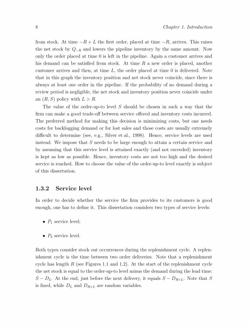
Both types consider stock out occurrences during the replenishment cycle. A replen-
ishment cycle is the time between two order deliveries. Note that a replenishment
cycle has length R (see Figures 1.1 and 1.2). At the start of the replenishment cycle
the net stock is equal to the order-up-to level minus the demand during the lead time:
S −DL. At the end, just before the next delivery, it equals S −DR+L. Note that S
is fixed, while DL and DR+L are random variables.

1.3. Introduction to the (R, S) policy and service levels 9
P1 service level
The P1 service level measures the fraction of replenishment cycles without stock out
occurrences. In literature it is also referred to as cycle service. Both terms are used
in this dissertation, as well as the notation α. Mathematically, the P1 service level is
defined as:
α = P (DR+L ≤ S) . (1.2)
Example 1.1 (P1 service)
Assume that demand during review plus lead time is distributed according to:
dR+L 15 25 35 45P (DR+L = dR+L)
18
38
38
18
.
If we set the order-up-to level to 25 (S = 25), the P1 service is
αS=25 = P (DR+L ≤ 25) =4
8= 0.50.
If we set the order-up-to level to 35, the P1 service is
αS=35 = P (DR+L ≤ 35) =7
8= 0.8750.
�
P2 service level
The P2 service level measures the fraction of demand satisfied directly from shelf. In
literature it is often referred to as fill rate. Both terms are used in this dissertation,
as well as the notation β. Mathematically, the P2 service level is defined as:
β = 1− E [(DR+L − S)+]− E [(DL − S)+]
E [DR]. (1.3)
The second term in the numerator prevents counting backlog twice: if there is already
a backlog at the start of the replenishment cycle, this should be subtracted from the
backlog at the end of the replenishment cycle. This second term is not always taken
into account in literature, mostly since the probability of having backlog at the start
of a replenishment cycle is negligible if the desired service level is high, which is
common in practice.

10 Chapter 1. Introduction
Example 1.2 (P2 service)
Assume that demand during lead time is distributed according to
dL 5 15
P (DL = dL)12
12
,
the demand during the review period according to
dR 10 20 30
P (DR = dR)14
24
14
,
and the demand during the review plus lead time according to
dR+L 15 25 35 45
P (DR+L = dR+L)18
38
38
18
.
If we set the order-up-to level to 25 (S = 25), the P2 service is determined by
E[(DR+L − 25)+
]= (35− 25) · 3
8+ (45− 25) · 1
8=
50
8E[(DL − 25)+
]= 0
E [DR] = 10 · 14+ 20 · 2
4+ 30 · 1
4= 20
βS=25 = 1−508− 0
20=
11
16= 0.6875.
If we set the order-up-to level to 35, the P2 service is
E[(DR+L − 35)+
]= (45− 35) · 1
8=
10
8E[(DL − 35)+
]= 0
E [DR] = 10 · 14+ 20 · 2
4+ 30 · 1
4= 20
βS=35 = 1−108− 0
20=
15
16= 0.9375.
�
One can think of many more service level definitions, for example the fraction of time
the net stock is positive or the probability that an arbitrary customer has to wait.
This dissertation focuses on the P1 and P2 service levels. One cannot say that one
of the two is better without knowing anything about the product and its market.
Consider the following two examples.

1.3. Introduction to the (R, S) policy and service levels 11
Example 1.3 (P1 versus P2 service (1))
A shop sells office supplies. The demand for a set of pens in the past ten days is
given below.
day 1 2 3 4 5 6 7 8 9 10demand 90 92 88 91 88 86 93 89 91 92
The store has an (R, S) policy, with the review period equal to one day (R = 1) and
the order-up-to level equal to 90 (S = 90). Its lead time is 0: the order is made after
closing and delivered the next morning before opening again.
The attained P1 service level in the past 10 days is only 0.50, while the attained
P2 service level is 0.99. In this case one could argue that the P2 service level is more
suitable, since the shopkeeper is more interested in the amount of demand he can
satisfy directly. He does not mind too much whether he can satisfy all the demand
during one day or not, as long as he satisfies most of the demand. �
Example 1.4 (P1 versus P2 service (2))
A maintenance department of a big factory has inventory of spare parts. The demand
for a certain spare part in the past ten days is given below.
day 1 2 3 4 5 6 7 8 9 10demand 7 11 8 12 9 9 13 9 12 10
The store has an (R, S) policy, with the review period equal to one day (R = 1) and
the order-up-to level equal to 9 (S = 9). Its lead time is 0: the order is made after
the end of the last shift and delivered the next morning before the first shift starts.
The attained P1 service level in the past 10 days is only 0.50, while the attained
P2 service level is 0.91. In this case one could argue that the P1 service level is more
suitable, since it is important that all the demand in a replenishment cycle is satisfied.
If a certain spare part is not available, a machine does not work and a factory cannot
produce, hence the factory does not generate revenue. �
So the P1 service level is best suited for situations in which missing one item is just
as bad as missing multiple items, e.g., spare parts. The P2 service suits situations
in which the amount of nonsatisfied demand is important, e.g., retail stores and
wholesale business.

12 Chapter 1. Introduction
1.4 Contributions and overview
The remainder of this dissertation is split into two parts. The first part, consisting of
Chapter 2, deals with modified demand distributions. This is an example of situation
(b), since we assume that we do know the mean, variance and third moment of
demand. In this part the demand follows a non-standard distribution and we show the
effect of using a wrong distribution (fitted with help of the mean, variance and third
moment of the demand) on the achieved performance. The second part, consisting
of Chapters 3–5, considers situation (a): not knowing the exact characteristics of
demand. In classic inventory control demand distribution is assumed to be known
completely. In practice this is rarely true. A demand distribution is assumed and
its parameters are estimated using historical demand observations. The effect of
replacing true, but unknown, parameters by their estimates is subject of the second
part. Chapter 6 concludes this dissertation.
Chapter 2 defines two modified shifted gamma distributions to be used in in-
ventory control. It provides a method to find the order-up-to levels under the new
demand distribution and compares the results to the regular and shifted gamma dis-
tribution.The main contribution of this chapter lies in providing demand distributions
that are more flexible.
Chapter 3 considers demand with a normal distribution with unknown parame-
ters. Under strong assumptions it is shown analytically that the desired service level
is not met when using estimates instead of the true parameters. When these assump-
tions are relieved, analytical derivations are no longer possible, but simulation shows
that also now the desired service is not met. This chapter provides a method that
improves the attained service and assures that the desired service is (almost) met.
The method is based on the analytical proof of not reaching the desired service and
on a regression technique. The main contributions of this chapter are the analytical
proof of not reaching the desired service level, and the development of a correction
function.
Chapter 4 considers demand with a gamma distribution with unknown parame-
ters. Also in this case the desired service level is not met when using estimates. This
is shown analytically under strong conditions and with simulation if these conditions
are relieved. A method that improves the attained service, based on analytical deriva-
tions and regression, is provided. Simulation shows that the desired service level is
(almost) met. The main contributions in this chapter are the analytical proof of not

1.4. Contributions and overview 13
reaching the desired service level, and the development of the correction functions.
Chapter 5 is more general compared to Chapters 3 and 4. An effect of estimating
the demand parameters is that the order-up-to level becomes a random variable (see
Sections 3.2 and 4.2.1). This chapter takes this given as a starting-point: the order-
up-to level is a random variable instead of a fixed number, as are the length of the
review period and the length of the lead time. The order-up-to level, the demand
during the review period and the demand during the lead time follow a mixed-Erlang
distribution. It is shown that the desired service level is not met when ignoring
the randomness. The correct order-up-to levels are derived analytically. The main
contribution in this chapter is simultaneously considering demand, the length of the
review period, the length of the lead time, and the order-up-to level to be random.
Chapter 6 provides the overall conclusion and directions for further research.


Part I
Modified distributions


Chapter 2
Modified shifted gammadistributions
This chapter considers the shifted gamma distribution: the gamma dis-tribution that also has a location parameter. If we assume that demandis distributed according to this gamma distribution, negative demand ob-servations may occur, which is often not realistic in practice. The twomodified shifted gamma distributions discussed in this chapter only havenonnegative values. Assuming that demand is distributed according to themodified shifted gamma distribution, the order-up-to level in an (R, S) in-ventory control policy is derived under the P1 and under the P2 servicelevel constraint. Finally, the results are compared to using a regular orshifted gamma distribution, while the true distribution is one of the twomodified shifted gamma distributions.
2.1 Introduction
The normal distribution is often used to model demand, because of its tractability
(see also Sections 1.1 and 3.1). The two main problems with this distribution are
that it is symmetric, and the probability of negative realizations is non-negligible
(more than 1%) if the coefficient of variation is larger than 0.43. In practice, demand
is often skewed to the right and, more important, negative demand hardly ever oc-
curs. Strijbosch and Moors (2006) have solved these two problems by constructing
two modified normal distributions: one with a point mass at zero and one truncated
at zero. These two modified normal distributions are skewed to the right and cannot
have negative realizations. They discuss these new distributions and their limitations
(the coefficient of variation cannot be large). Furthermore, they use these distribu-

18 Chapter 2. Modified shifted gamma distributions
tions to model the demand in an (R, S) inventory control policy with cycle service
and fill rate constraints. Finally, they show that using the regular normal distribution
while in fact the demand is distributed according to a modified normal distribution
leads to underperformance. The modified normal distribution with a point mass at
zero has the nice side-effect that it can be used as the distribution of intermittent
demand, since the probability of zero demand is positive. Intermittent demand is
often modeled using a compound distribution: the demand occurrences follow some
distribution, e.g., the Bernoulli distribution, and the demand sizes follow another
distribution, e.g., the gamma distribution; see, e.g., Janssen et al. (1998). Thus, we
need two distributions to model the intermittent demand if we use the compound
distribution approach, whereas one of the modified normal distributions captures the
intermittency directly.
Another way to capture the nonnegativity of demand is using the gamma distribu-
tion to model demand (see also Section 4.1). This distribution does not have negative
realizations and, furthermore, it is skewed to the right. Also the gamma distribution
is easy to work with, although it does not have all the nice properties of the normal
distribution. A disadvantage is that the probability of having zero demand is zero,
and therefore this distribution cannot be used for intermittent demand.
Starting from the regular gamma distribution one can construct a shifted gamma
distribution, simply by shifting the complete pdf either to the left or to the right. If it
is shifted to the left, negative realizations can occur and we can use this shifted gamma
distribution to construct two modified shifted gamma distributions, analogously to
Strijbosch and Moors (2006).
These two modified shifted gamma distributions have the major advantage that
they are more flexible than the regular gamma distribution, since the modified shifted
gamma distribution has three parameters instead of the two parameters of the regular
gamma distribution. Furthermore, the modified shifted gamma distribution with a
point mass at zero can be used to directly model intermittent demand, since the
probability of having zero demand is positive.
These two modified shifted gamma distribution are used to model demand during
review in an (R, S) inventory control policy with lead time equal to zero. So, every R
periods the inventory position is replenished up to the order-up-to level S and that
order is delivered instantaneously. The size of the order-up-to level is chosen such
that either the cycle service or the fill rate reaches a prescribed value. Note that the
assumption of zero lead time is not as rigid as it might seem at first sight. Consider,
2.2. Modified normal distribution 19
e.g., a supermarket that makes its order at the end of opening hours and receives
this order the next morning before opening hours. The time it takes the supplier to
deliver is then approximately 12 hours (depending on the opening hours), but since
the supermarket is closed during that time, one can take the lead time equal to zero.
This chapter starts with a summary of the results obtained by Strijbosch and
Moors (2006) (the use of modified normal distributions to model demand). Next,
the shifted gamma distribution is defined and also the two modified shifted gamma
distributions are constructed from this shifted gamma distribution. In Section 2.4 the
order-up-to levels under the modified shifted gamma distributions are derived and
some general results considering the order-up-to levels using modified distributions
are provided. Section 2.5 considers the use of the regular and modified gamma
distribution, while demand actually follows a modified gamma distribution. This
chapter is concluded in Section 2.6.
2.2 Modified normal distribution
Strijbosch and Moors (2006) have introduced two modified normal distributions, that
only consider nonnegative observations. They start from the regular normal distri-
bution with pdf fµ,σ2(x) and cdf Fµ,σ2(x).
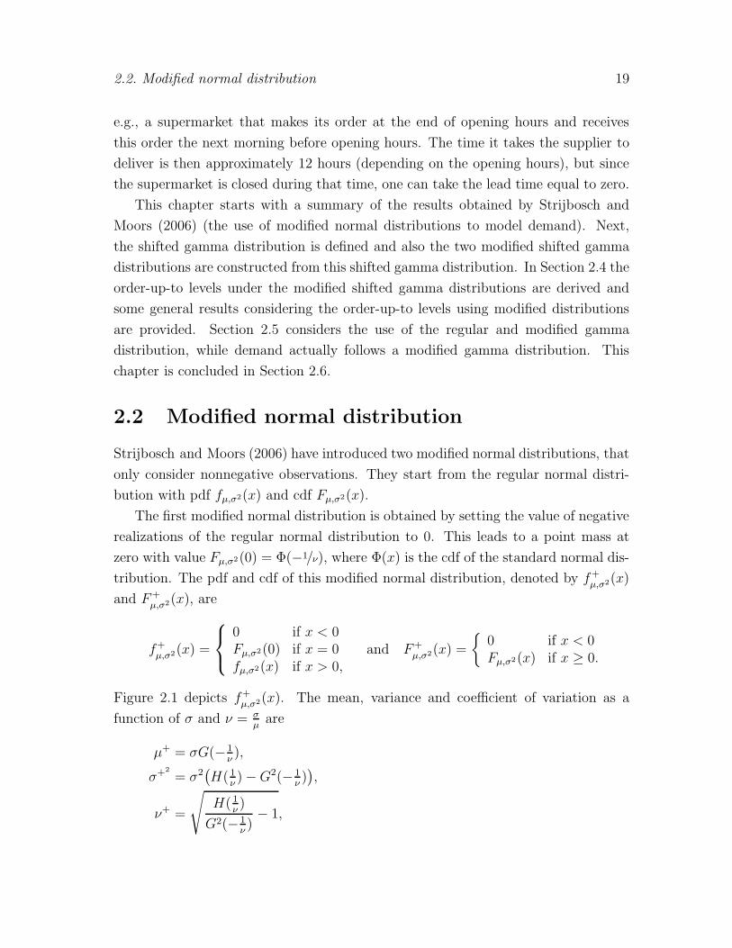
The first modified normal distribution is obtained by setting the value of negative
realizations of the regular normal distribution to 0. This leads to a point mass at
zero with value Fµ,σ2(0) = Φ(−1/ν), where Φ(x) is the cdf of the standard normal dis-
tribution. The pdf and cdf of this modified normal distribution, denoted by f+µ,σ2(x)
and F+µ,σ2(x), are
f+µ,σ2(x) =
0 if x < 0Fµ,σ2(0) if x = 0fµ,σ2(x) if x > 0,
and F+µ,σ2(x) =
{0 if x < 0Fµ,σ2(x) if x ≥ 0.
Figure 2.1 depicts f+µ,σ2(x). The mean, variance and coefficient of variation as a
function of σ and ν = σµare
µ+ = σG(− 1ν),
σ+2
= σ2(H( 1
ν)−G2(− 1
ν)),
ν+ =
√H( 1
ν)
G2(− 1ν)− 1,

20 Chapter 2. Modified shifted gamma distributions
Fµ,σ2(0)
σ
f+µ,σ2(x)
fµ,σ2(x)
x →0 µ
Figure 2.1: The pdf of a modified normal distribution with a point mass at zero (f+µ,σ2).
where G(x) denotes the loss function of a standard normal variate, i.e.,
G(x) = E[(Z − x)+
]=
∫ ∞
x
(z − x)ϕ(z)dz = ϕ(x)− xΦ(−x),
and H(x) is an auxiliary function, which denotes
H(x) = xϕ(x) + (x2 + 1)Φ(x).
Finally, ϕ(x) and Φ(x) are the pdf and cdf of a standard normal variate.
The second modified normal distribution is constructed by ignoring all negative
realizations of a regular normal distribution; this is a normal distribution truncated
at zero. The pdf and cdf (f ∗µ,σ2(x) and F ∗
µ,σ2(x)) of this truncated normal distribution
are
f ∗µ,σ2(x) =
0 if x < 0fµ,σ2(x)
Φ(1ν
) if x ≥ 0,and F ∗
µ,σ2(x) =
0 if x < 0Fµ,σ2(x)− Φ
(− 1
ν
)
Φ(1ν
) if x ≥ 0.
The pdf belonging to the truncated normal distribution is depicted in Figure 2.2. The
mean, variance and coefficient of variation belonging to this modified distribution,
are
µ∗ = σG(− 1
ν)
Φ( 1ν),
σ∗2 = σ2Φ(1ν)H( 1
ν)−G2(− 1
ν)
Φ2( 1ν)
,
ν∗ =
√Φ( 1
ν)H( 1
ν)
G(− 1ν)
− 1.
2.2. Modified normal distribution 21
σ
f ∗µ,σ2(x)
fµ,σ2(x)
x →0 µ
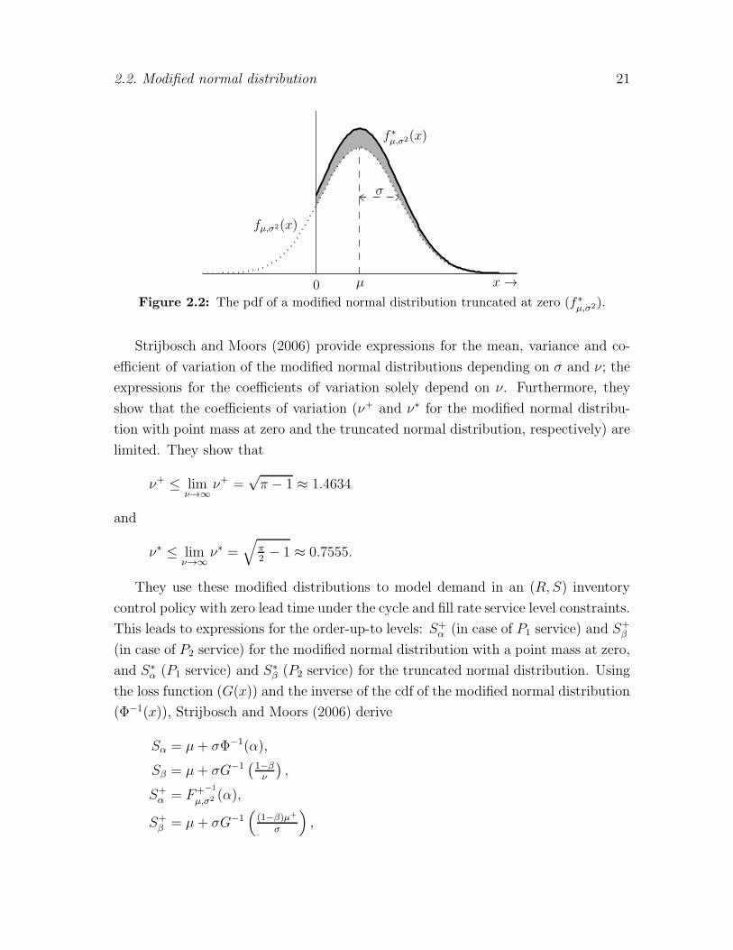
Figure 2.2: The pdf of a modified normal distribution truncated at zero (f∗µ,σ2).
Strijbosch and Moors (2006) provide expressions for the mean, variance and co-
efficient of variation of the modified normal distributions depending on σ and ν; the
expressions for the coefficients of variation solely depend on ν. Furthermore, they
show that the coefficients of variation (ν+ and ν∗ for the modified normal distribu-
tion with point mass at zero and the truncated normal distribution, respectively) are
limited. They show that
ν+ ≤ limν→∞
ν+ =√π − 1 ≈ 1.4634
and
ν∗ ≤ limν→∞
ν∗ =√
π2− 1 ≈ 0.7555.
They use these modified distributions to model demand in an (R, S) inventory
control policy with zero lead time under the cycle and fill rate service level constraints.
This leads to expressions for the order-up-to levels: S+α (in case of P1 service) and S+
β
(in case of P2 service) for the modified normal distribution with a point mass at zero,
and S∗α (P1 service) and S∗
β (P2 service) for the truncated normal distribution. Using
the loss function (G(x)) and the inverse of the cdf of the modified normal distribution
(Φ−1(x)), Strijbosch and Moors (2006) derive
Sα = µ+ σΦ−1(α),
Sβ = µ+ σG−1(1−βν
),
S+α = F+−1
µ,σ2 (α),
S+β = µ+ σG−1
((1−β)µ+
σ
),

22 Chapter 2. Modified shifted gamma distributions
S∗α = µ+ σΦ−1
(α + (1− α)Φ
(− 1
ν
)),
S∗β = µ+ σG−1
((1−β)µ∗Φ
(1ν
)
σ
),
where Sα and Sβ are the well-known order-up-to levels using a regular normal dis-
tribution. Using the order-up-to levels as defined above and the expressions for µ+
and µ∗, it is easily shown that
S+α = Sα and S∗
β = S+β .
Furthermore, it holds that
S∗α > Sα and S+
β < Sβ.
Section 2.4 shows that these properties also hold for the modified gamma distribu-
tions and, in fact, for general modified distributions constructed in an analogous way
(Section 2.4.3).
Finally, Strijbosch and Moors (2006) show the consequences of using a regular
normal distribution while in fact the demand is distributed according to the modi-
fied normal distribution: the desired service level is not reached and the larger the
coefficient of variation is, the larger the underperformance is.
2.3 Modified shifted gamma distributions
This chapter considers two modified shifted gamma distributions, that start from
the shifted gamma distribution. This distribution is also known as a Pearson type
III distribution or a three-parameter gamma distribution, although there are also
references to other three-parameter gamma distributions, so the latter is not uniquely
defined. The shifted gamma distribution has three parameters: a location parameter
∆, a shape parameter ρ and a scale parameter θ. Its pdf (fρ,θ,∆(x)) and cdf (Fρ,θ,∆(x))
are defined as
fρ,θ,∆(x) =
(x+∆)ρ−1e−x+∆θ
θρΓ(ρ)if x ≥ −∆
0 if x < −∆
=
{fρ,θ(x+∆) if x ≥ −∆0 if x < −∆,
Fρ,θ,∆(x) =
{Fρ,θ(x+∆) if x ≥ −∆0 if x < −∆,

2.3. Modified shifted gamma distributions 23
where fρ,θ(x) and Fρ,θ(x) denote the pdf and cdf of a regular gamma distribution
(the shifted gamma distribution with ∆ = 0) and Γ(x) denotes the gamma function.
Figure 2.3 displays the pdf of a shifted gamma distribution and a regular gamma
distribution with the same shape and scale parameter. Note that, in order to obtain
x →0−∆
fρ,θ(x)
fρ,θ,∆(x)
Figure 2.3: The pdf of a shifted gamma distribution, with probability of negative realiza-tions depicted in gray, compared to the regular gamma distribution
the pdf of the shifted gamma distribution, the complete pdf of the regular gamma
distribution with the same scale and shape parameters shifts ∆ to the left. The mean
and variance of a regular gamma distribution are ρθ and ρθ2; the mean and variance
of the shifted gamma distribution are easily obtained using the shift of size ∆:
µ = ρθ −∆,
σ2 = ρθ2,
ν =σ
µ=
√ρθ
ρθ −∆.
Two important results from the regular gamma distribution can be translated to
the shifted gamma distribution:
Gρ,θ,∆(x) =
∫ ∞
x
(z − x)fρ,θ,∆(z)dz
= ρθ[1 − Fρ+1,θ,∆(x)]− (x+∆)[1− Fρ,θ,∆(x)], (2.1)
xfρ,θ,∆(x) = θρfρ+1,θ,∆(x)−∆fρ,θ,∆(x). (2.2)
The derivations of (2.1) and (2.2) are in Appendix A.1. Using (2.2), we obtain the
24 Chapter 2. Modified shifted gamma distributions
following two expressions:
x2fρ,θ,∆(x) = θ2ρ(ρ+ 1)fρ+2,θ,∆(x)− 2∆θρfρ+1,θ,∆(x) + ∆2fρ,θ,∆(x), (2.3)
x3fρ,θ,∆(x) = θ3ρ(ρ+ 1)(ρ+ 2)fρ+3,θ,∆(x)− 3∆θ2ρ(ρ+ 1)fρ+2,θ,∆(x)
+ 3∆2θρfρ+1,θ,∆(x)−∆3fρ,θ,∆(x). (2.4)
Equation (2.3) is obtained by multiplying both the left-hand side and right-hand side
of (2.2) by x and using (2.2) on the right-hand side again. Equation (2.4) is derived
by multiplying both the left-hand side and right-hand side of (2.3) by x and using
(2.2) on the right-hand side again. The exact derivations are also in A.1.
In general, the location parameter ∆ could have any value, but since we start
from a distribution with possibly negative realizations, ∆ is assumed to be positive
in the remainder of this chapter.
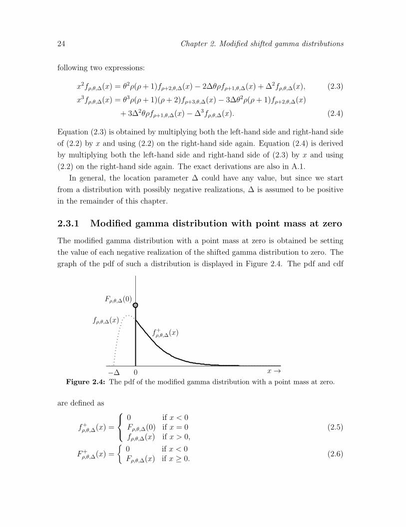
2.3.1 Modified gamma distribution with point mass at zero
The modified gamma distribution with a point mass at zero is obtained be setting
the value of each negative realization of the shifted gamma distribution to zero. The
graph of the pdf of such a distribution is displayed in Figure 2.4. The pdf and cdf
x →0−∆
f+ρ,θ,∆(x)
fρ,θ,∆(x)
Fρ,θ,∆(0)
Figure 2.4: The pdf of the modified gamma distribution with a point mass at zero.
are defined as
f+ρ,θ,∆(x) =
0 if x < 0Fρ,θ,∆(0) if x = 0fρ,θ,∆(x) if x > 0,
(2.5)
F+ρ,θ,∆(x) =
{0 if x < 0Fρ,θ,∆(x) if x ≥ 0.
(2.6)

2.3. Modified shifted gamma distributions 25
The mean of this distribution, denoted by µ+, is
µ+ =
∫ ∞
0
xf+ρ,θ,∆(x)dx = 0 · Fρ,θ,∆(0) +
∫ ∞
0
xfρ,θ,∆(x)dx = Gρ,θ,∆(0).
The second moment, denoted by µ+2 , is
µ+2 =
∫ ∞
0
x2f+ρ,θ,∆(x)dx = 02 · Fρ,θ,∆(0) +
∫ ∞
0
x2fρ,θ,∆(x)dx =
∫ ∞
0
x2fρ,θ,∆(x)dx
(2.3)=
∫ ∞
0
(θ2ρ(ρ+ 1)fρ+2,θ,∆(x)− 2∆θρfρ+1,θ,∆(x) + ∆2fρ,θ,∆(x)
)dx
= θ2ρ(ρ+ 1)(1− Fρ+2,θ,∆(0)
)− 2∆θρ
(1− Fρ+1,θ,∆(0)
)+∆2
(1− Fρ,θ,∆(0)
)
= θρGρ+1,θ,∆(0)−∆Gρ,θ,∆(0).
We will need the third moment in Section 2.5; the third moment, µ+3 , is
µ+3 =
∫ ∞
0
x3f+ρ,θ,∆(x)dx = 03 · Fρ,θ,∆(0) +
∫ ∞
0
x3fρ,θ,∆(x)dx =
∫ ∞
0
x3fρ,θ,∆(x)dx
(2.4)=
∫ ∞
0
(θ3ρ(ρ+ 1)(ρ+ 2)fρ+3,θ,∆(x)− 3∆θ2ρ(ρ+ 1)fρ+2,θ,∆(x)
+ 3∆2θρfρ+1,θ,∆(x)−∆3fρ,θ,∆(x))dx
= θ3ρ(ρ+ 1)(ρ+ 2)(1− Fρ+3,θ,∆(0)
)− 3∆θ2ρ(ρ+ 1)
(1− Fρ+2,θ,∆(0)
)
+ 3∆2θρ(1− Fρ+1,θ,∆(0)
)−∆3
(1− Fρ,θ,∆(0)
)
= θ2ρ(ρ+ 1)Gρ+2,θ,∆(0)− 2∆θρGρ+1,θ,∆(0) + ∆2Gρ,θ,∆(0).
The variance of a modified gamma distributed variable with a point mass at zero,
denoted by σ+2
, is
σ+2
= µ+2 − (µ+)2 = ρθGρ+1,θ,∆(0)−∆Gρ,θ,∆(0)−G2
ρ,θ,∆(0)
= θ2ρ(ρ+ 1)(1− Fρ+2,θ,∆(0)
)− 2∆ρθ
(1− Fρ+1,θ,∆(0)
)+∆2
(1− Fρ,θ,∆(0)
)
−(ρ2θ2
(1− Fρ+1,θ,∆(0)
)2
− 2ρθ∆(1− Fρ+1,θ,∆(0)
)(1− Fρ,θ,∆(0)
)+∆2
(1− Fρ,θ,∆(0)
)2)
= θ2ρ(ρ+ 1)(1− Fρ+2,θ,∆(0)
)+∆2
(1− Fρ,θ,∆(0)
)(1−
(1− Fρ,θ,∆(0)
))
− ρθ(1− Fρ+1,θ,∆(0)
)(2∆ + ρθ
(1− Fρ+1,θ,∆(0)
)− 2∆
(1− Fρ,θ,∆(0)
))
= θ2ρ(ρ+ 1)(1− Fρ+2,θ,∆(0)
)+∆2Fρ,θ,∆(0)
(1− Fρ,θ,∆(0)
)
− ρθ(1− Fρ,θ,∆(0)
)(ρθ(1− Fρ+1,θ,∆(0)
)+ 2∆
(1−
(1− Fρ,θ,∆(0)
)))

26 Chapter 2. Modified shifted gamma distributions
= θ2ρ(ρ+ 1)(1− Fρ+2,θ,∆(0)
)+∆2Fρ,θ,∆(0)
(1− Fρ,θ,∆(0)
)
− ρθ(1− Fρ,θ,∆(0)
)(ρθ(1− Fρ+1,θ,∆(0)
)+ 2∆Fρ,θ,∆(0)
).
Finally, the coefficient of variation, denoted by ν+, is
ν+ =
√ρθGρ+1,θ,∆(0)−∆Gρ,θ,∆(0)−G2
ρ,θ,∆(0)
Gρ,ρ∆(0).
2.3.2 Modified gamma distribution truncated at zero
The modified gamma distribution truncated at zero is obtained by ignoring negative
realizations of the shifted gamma distribution. The graph of the pdf belonging to
the modified gamma distribution that is truncated at zero, is provided in Figure 2.5.
The pdf and cdf of this modified distribution, denoted by f ∗ρ,θ,∆ and F ∗
ρ,θ,∆, are
x →0−∆
f ∗ρ,θ,∆(x)
fρ,θ,∆(x)
Figure 2.5: The pdf of the modified gamma distribution truncated at zero.
f ∗ρ,θ,∆(x) =
0 if x < 0fρ,θ,∆(x)
1− Fρ,θ,∆(0)if x ≥ 0,
(2.7)
F ∗ρ,θ,∆(x) =
0 if x < 0Fρ,θ,∆(x)− Fρ,θ,∆(0)
1− Fρ,θ,∆(0)if x ≥ 0.
(2.8)
Let P denote 1−Fρ,θ,∆(0). Then the kth moment of the modified shifted gamma
distribution truncated at zero, denoted by µ∗k, is
µ∗k =
∫ ∞
0
xkf ∗ρ,θ,∆(x)dx =
∫ ∞
0
xk fρ,θ,∆(x)
P dx =1
P
∫ ∞
0
xkfρ,θ,∆(x)dx =µ+k
P .
2.4. Determination of order-up-to levels 27
Hence, the expected value, and the second and third moment of the truncated shifted
gamma distribution are
µ∗ =µ+
P , µ∗2 =
µ+2
P , and µ∗3 =
µ+3
P .
The variance of a truncated shifted gamma distribution, denoted by σ∗2 , is
σ∗2 = µ∗2 − (µ∗)2 =
µ+2
P − (µ+)2
P2=
(1− Fρ,θ,∆(0)
)µ+2 − (µ+)2
P2
=
(1− Fρ,θ,∆(0)
)(θ2ρ(ρ+ 1)
(1− Fρ+2,θ,∆(0)
)+∆2
(1− Fρ,θ,∆(0)
))
P2
+
(1− Fρ,θ,∆(0)
)(− 2∆θρ
(1− Fρ+1,θ,∆(0)
))− ρ2θ2
(1− Fρ+1,θ,∆(0)
)2
P2
+2ρθ∆
(1− Fρ+1,θ,∆(0)
)(1− Fρ,θ,∆(0)
)−∆2
(1− Fρ,θ,∆(0)
)2
P2
=θ2ρ(ρ+ 1)
(1− Fρ,θ,∆(0)
)(1− Fρ+2,θ,∆(0)
)+∆2
(1− Fρ,θ,∆(0)
)2
P2
+−2∆θρ
(1− Fρ+1,θ,∆(0)
)(1− Fρ,θ,∆(0)
)− ρ2θ2
(1− Fρ+1,θ,∆(0)
)2
P2
+2ρθ∆
(1− Fρ+1,θ,∆(0)
)(1− Fρ,θ,∆(0)
)−∆2
(1− Fρ,θ,∆(0)
)2
P2
=θ2ρ(ρ+ 1)
(1− Fρ,θ,∆(0)
)(1− Fρ+2,θ,∆(0)
)− ρ2θ2
(1− Fρ+1,θ,∆(0)
)2
P2.
The coefficient of variation, ν∗, is
ν∗ =θ√ρ√(ρ+ 1)
(1− Fρ,θ,∆(0)
)(1− Fρ+2,θ,∆(0)
)− ρ(1− Fρ+1,θ,∆(0)
)2
µ+
=θ√ρ√(ρ+ 1)
(1− Fρ,θ,∆(0)
)(1− Fρ+2,θ,∆(0)
)− ρ(1− Fρ+1,θ,∆(0)
)2
ρθ(1− Fρ+1,θ,∆(0)
)−∆
(1− Fρ,θ,∆(0)
) .
2.4 Determination of order-up-to levels
First, we derive the order-up-to levels for the shifted gamma distribution, since this
distribution is not widely applied in inventory control. We consider both the P1
service criterion and the P2 service criterion.
28 Chapter 2. Modified shifted gamma distributions
If the demand, denoted by D, is shifted gamma distributed with demand parame-
ters ρ, θ and ∆, the order-up-to level under the P1 criterion, denoted by Sα, is found
by solving
P (D ≤ Sα) = α.
Using that Fρ,θ,∆(Sα) = P (D ≤ Sα), we obtain
Sα = F−1ρ,θ,∆(α).
If the fill rate criterion is considered, the order-up-to level, Sβ, is determined by
solving
1− E [(D − Sβ)+]
E [D]= 1− E [(D − Sβ)
+]
µ= β.
Rewriting the above and using (2.1) leads to the following expression for the order-
up-to level:
(1− β)µ = E[(D − Sβ)
+]=
∫ ∞
Sβ
(x− Sβ)fρ,θ,∆(x)dx = Gρ,θ,∆(Sβ),
Sβ = G−1ρ,θ,∆((1− β)µ).
2.4.1 Using F+ρ,θ,∆
Let us now assume that demand (D) is distributed according to a modified shifted
gamma distribution with a point mass at zero with parameters ρ, θ and ∆. The
order-up-to level using the cycle service criterion, denoted by S+α is obtained by
solving
P(D ≤ S+
α
)= α.
The order-up-to level under the P1 service level is
S+α = F+−1
ρ,θ,∆(α)(∗)= F−1
ρ,θ,∆(α) = Sα.
Note that the equality at (∗) is obtained using (2.6) and that it implicitly assumes
that α > Fρ,θ,∆(0). This is not a limitation in practice, since there will not be many
SKUs (an SKU is a stock-keeping unit) that have a probability of zero demand that
is higher than the desired service level.

2.4. Determination of order-up-to levels 29
If we consider the P2 service level criterion, the order-up-to level S+β needs to
satisfy
1−E[(D − S+
β )+]
E [D]= 1−
E[(D − S+
β )+]
µ+= β.
Rewriting and using both (2.5) and (2.1) leads to
(1− β)µ+ = E[(D − S+
β )+]=
∫ ∞
S+
β
(x− S+β )f
+ρ,θ,∆(x)dx
=
∫ ∞
S+
β
(x− S+β )fρ,θ,∆(x)dx = Gρ,θ,∆(S
+β ),
S+β = G−1
ρ,θ,∆((1− β)µ+) < Sβ.
We implicitly assumed that S+β > 0, which is a reasonable assumption in practice;
there will not be many SKUs that have negative order-up-to levels. Furthermore,
the inequality is obtained from the fact that µ+ > µ and G−1ρ,θ,∆(x) is a decreasing
function, as Gρ,θ,∆(x) is a decreasing function.
2.4.2 Using F ∗
ρ,θ,∆
Let us now assume that demand D is distributed according to a truncated shifted
gamma distribution with parameters ρ, θ and ∆. As before, let P = 1−Fρ,θ,∆(0) for
brevity. The order-up-to level under the P1 service level, S∗α, is found by solving
P (D ≤ S∗α) = α.
Rewriting and using (2.8) leads to
F ∗ρ,θ,∆(S
∗α) =
Fρ,θ,∆(S∗α)− Fρ,θ,∆(0)
P = α,
Fρ,θ,∆(S∗α) = αP + Fρ,θ,∆(0) = α(1− Fρ,θ,∆(0)) + Fρ,θ,∆(0)
= α + (1− α)Fρ,θ,∆(0),
S∗α = F−1
ρ,θ,∆(α + (1− α)Fρ,θ,∆(0)) > Sα = S+α .
The inequality is obtained by noting that α+(1−α)Fρ,θ,∆(0) > α and that Fρ,θ,∆(x)
is an increasing function, and therefore also F−1ρ,θ,∆(x) is. Again, we need that the
order-up-to level is positive.

30 Chapter 2. Modified shifted gamma distributions
If a fill rate criterion is used, the order-up-to level, denoted by S∗β, is determined
using
1−E[(D − S∗
β)+]
E [D]= 1−
E[(D − S∗
β)+]
µ∗ = β.
Rewriting the above and using (2.7) provides an expression for the order-up-to level,
namely
(1− β)µ∗ = E[(D − S+
β )∗] =
∫ ∞
S∗
β
(x− S∗β)f
∗ρ,θ,∆(x)dx
=
∫ ∞
S∗
β
(x− S∗β)fρ,θ,∆(x)
P dx =1
PGρ,θ,∆(S∗β),
S∗β = G−1
ρ,θ,∆((1− β)µ∗P)(∗)= G−1
ρ,θ,∆((1− β)µ+) = S+β .
Also here we need that S∗β > 0. For the equality at (∗) we use that µ∗ = µ+
P . Note
that since S+β < Sβ it also holds that S∗
β < Sβ.
2.4.3 Results with general distributions
Note that for both the modified normal distribution and the modified shifted gamma
distribution the following properties for the order-up-to levels hold (see Sections 2.2
and 2.4):
S+α = Sα ≤ S∗
α,S∗β = S+
β ≤ Sβ.(2.9)
In the remainder of this section it is proven to be true for any modified distribution
constructed in the same way.
Let f(x) and F (x) be a general density and distribution function of a continuous
distribution. Now let us construct the two modified distributions f+(x) and F+(x),
and f ∗(x) and F ∗(x); the first has a point mass at zero with probability F (0) and the
second is truncated at zero. The pdf and cdf of the distribution with a point mass
are defined as follows:
f+(x) =
0 if x < 0F (0) if x = 0f(x) if x > 0,
and F+(x) =
{0 if x < 0F (x) if x ≥ 0.
The pdf and cdf of the truncated distribution are
f ∗(x) =
0 if x < 0f(x)
1− F (0)if x ≥ 0,
and F ∗(x) =
0 if x < 0F (x)− F (0)
1− F (0)if x ≥ 0.

2.4. Determination of order-up-to levels 31
Note that in case only nonnegative realizations are possible under the original dis-
tribution (so, if F (0) = 0), the original distribution and the modified distributions
coincide. In that case also the order-up-to levels coincide, hence the conjecture that
(2.9) will hold in general is trivial. Therefore, for the remainder of this section we
assume that F (0) > 0 and in that case strict inequalities will hold in (2.9).
Further, the expected value of the distribution with a point mass, denoted by µ+
is given by
µ+ =
∫ ∞
−∞xf+(x)dx = 0F (0) +
∫ ∞
0
xf(x)dx =
∫ ∞
0
xf(x)dx,
while the expected value of the truncated distribution, µ∗, is
µ∗ =
∫ ∞
−∞xf ∗(x)dx =
∫ ∞
0
xf(x)
1 − F (0)dx =
1
1− F (0)
∫ ∞
0
xf(x)dx.
Hence, µ∗ = µ+
1−F (0).
Let G(z) denote the loss function belonging to a variable X that is distributed
according to f(x), so
G(z) =
∫ ∞
z
(x− z)f(x)dx = E[(X − z)+
].
The order-up-to levels of the original distribution under the P1 and P2 service
equation, denoted by Sα and Sβ respectively, are
Sα = F−1(α),
Sβ = G−1((1− β)µ),
where µ denotes the expected value of the original distribution. Note that
µ =
∫ ∞
−∞xf(x)dx =
∫ 0
−∞xf(x)dx+
∫ ∞
0
xf(x)dx <
∫ ∞
0
xf(x)dx = µ+.
Now let us consider the case that demand (D) is distributed according to the
distribution with a point mass at zero. The order-up-to levels under the cycle service
and fill rate criterion are denoted by S+α and S+
β respectively. First consider the P1
service criterion. The order-up-to level is chosen such that
α = F+(S+α ) = F (S+
α ).

32 Chapter 2. Modified shifted gamma distributions
The order-up-to level is
S+α = F−1(α) = Sα,
so indeed S+α = Sα. For the fill rate service criterion the order-up-to level needs to
satisfy
1−E[(D − S+
β )+]
E [D]= 1−
E[(D − S+
β )+]
µ+= β.
The order-up-to level is obtained by rewriting:
(1− β)µ+ =
∫ ∞
S+
β
(x− S+β )f
+(x)dx
=
∫ ∞
S+
β
(x− S+β )f(x)dx = G(S+
β ),
S+β = G−1((1− β)µ+).
Since µ+ > µ andG(x) is a strictly decreasing function, we know that G−1((1−β)µ) >
G−1((1− β)µ+) and hence
S+β < Sβ .
Finally, let us consider the case that demand D is distributed according to the
truncated distribution. The order-up-to levels under the cycle service and fill rate
criterion are S∗α and S∗
β respectively. First, S∗α is chosen such that F ∗(S∗
α) = α.
Rewriting this leads to
F ∗(S∗α) =
F (S∗α)− F (0)
1− F (0)= α,
F (S∗α) = α(1− F (0)) + F (0) = α + (1− α)F (0),
S∗α = F−1(α + (1− α)F (0)).
Since α + (1 − α)F (0) > α and F (x) is a strictly increasing function, we know that
F−1(α + (1− α)F (0)) > F−1(α) and hence
S∗α > Sα.
Consider S∗β. This order-up-to level needs to satisfy 1 − E[(D−S∗
β)+]
E[D]= β; rewriting
provides us with
(1− β)µ∗ =
∫ ∞
S∗
β
(x− S∗β)f
∗(x)dx =
∫ ∞
S∗
β
(x− S∗β)
f(x)
1− F (0)dx =
1
1− F (0)G(S∗
β),
S∗β = G−1((1− β)µ∗(1− F (0))).
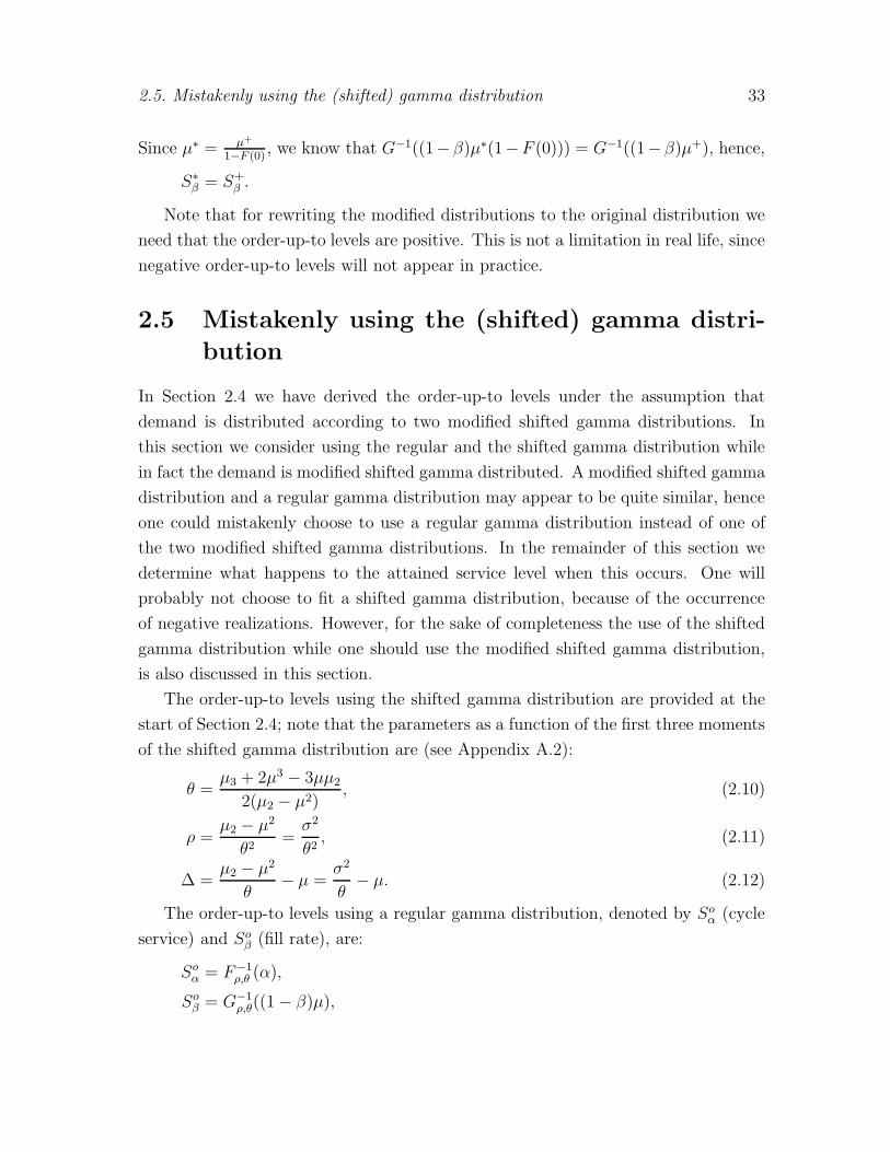
2.5. Mistakenly using the (shifted) gamma distribution 33
Since µ∗ = µ+
1−F (0), we know that G−1((1− β)µ∗(1−F (0))) = G−1((1− β)µ+), hence,
S∗β = S+
β .
Note that for rewriting the modified distributions to the original distribution we
need that the order-up-to levels are positive. This is not a limitation in real life, since
negative order-up-to levels will not appear in practice.
2.5 Mistakenly using the (shifted) gamma distri-
bution
In Section 2.4 we have derived the order-up-to levels under the assumption that
demand is distributed according to two modified shifted gamma distributions. In
this section we consider using the regular and the shifted gamma distribution while
in fact the demand is modified shifted gamma distributed. A modified shifted gamma
distribution and a regular gamma distribution may appear to be quite similar, hence
one could mistakenly choose to use a regular gamma distribution instead of one of
the two modified shifted gamma distributions. In the remainder of this section we
determine what happens to the attained service level when this occurs. One will
probably not choose to fit a shifted gamma distribution, because of the occurrence
of negative realizations. However, for the sake of completeness the use of the shifted
gamma distribution while one should use the modified shifted gamma distribution,
is also discussed in this section.
The order-up-to levels using the shifted gamma distribution are provided at the
start of Section 2.4; note that the parameters as a function of the first three moments
of the shifted gamma distribution are (see Appendix A.2):
θ =µ3 + 2µ3 − 3µµ2
2(µ2 − µ2), (2.10)
ρ =µ2 − µ2
θ2=
σ2
θ2, (2.11)
∆ =µ2 − µ2
θ− µ =
σ2
θ− µ. (2.12)
The order-up-to levels using a regular gamma distribution, denoted by Soα (cycle
service) and Soβ (fill rate), are:
Soα = F−1
ρ,θ (α),
Soβ = G−1
ρ,θ((1− β)µ),

34 Chapter 2. Modified shifted gamma distributions
where Fρ,θ = Fρ,θ,0 and Gρ,θ = Gρ,θ,0. The parameters as a function of the first two
moments are
θ =µ2 − µ2
µ=
σ2
µ, (2.13)
ρ =µ2
µ2 − µ2=
µ2
σ2. (2.14)
We first consider that demand is distributed according to the modified shifted
gamma distribution with a point mass at zero, next the truncated shifted gamma
distribution is considered.
2.5.1 Not using F+ρ,θ,∆
If we know that demand is distributed according the modified shifted gamma distri-
bution with a point mass at zero with demand parameters ρ, θ and ∆, the first three
moments are (see Section 2.3.1)
µ+ = Gρ,θ,∆(0),
µ+2 = θρGρ+1,θ,∆(0)−∆Gρ,θ,∆(0),
µ+3 = θ2ρ(ρ+ 1)Gρ+2,θ,∆(0)− 2∆θρGρ+1,θ,∆(0) + ∆2Gρ,θ,∆(0).
We can estimate the parameters of the shifted and regular gamma distribution by
substituting these three moments in (2.10)–(2.14). Let us denote these parameters
by θ+, ρ+ and ∆+ for the shifted gamma distribution, and θ+ and ρ+ for the regular
gamma distribution, so, e.g.,
θ+ =µ+3 + 2µ+3 − 3µ+µ+
2
2(µ+2 − µ+2)
.
This leads to the estimated order-up-to levels
S+α = F−1
ρ+,θ+,∆+(α),
S+β = G−1
ρ+,θ+,∆+((1− β)µ+),
S+α = F−1
ρ+,θ+(α),
S+β = G−1
ρ+,θ+((1− β)µ+).
Since the true demand distribution is known, we can also obtain the attained service
levels using the wrong order-up-to levels. The attained service using the shifted

2.5. Mistakenly using the (shifted) gamma distribution 35
gamma distribution, denoted by α+ and β+ for the P1 and P2 service level respectively,
is
α+ = F+ρ,θ,∆(S
+α ),
β+ = 1−Gρ,θ,∆(S
+β )
µ+.
Finally, the attained service levels using the regular gamma distribution, α+ and β+,
are
α+ = F+ρ,θ,∆(S
+α ),
β+ = 1−Gρ,θ,∆(S
+β )
µ+.
Figures 2.6–2.9 show the attained service level when using S+α , S+
β , S+α and S+
β ,
respectively, for two values of the desired service level, for three values of ρ, and for
different values of ∆. The value of θ is 10ρ
for all graphs. Also other values of θ
are used and these result in similar graphs (not shown here). Figure 2.6 shows the
∆
α
α = 0.90
ρ = 14
ρ = 1 ρ = 4
0 5 10 150.88
0.89
0.9
0.91
0.92
∆
α
α = 0.95
ρ = 14
ρ = 1 ρ = 4
0 5 10 150.93
0.94
0.95
0.96
Figure 2.6: Attained P1 service when using a shifted gamma distribution, while demandis distributed according to F+
ρ,θ,∆.
attained cycle service when using the shifted gamma distribution, while in fact the
demand is modified shifted gamma distributed with a point mass at zero. In both
the left graph (α = 0.90) and the right graph (α = 0.95) the attained service level
is close to the desired service level. In case of α = 0.95 the attained service is below
the desired service for all values of ∆, but the largest underperformance is less than
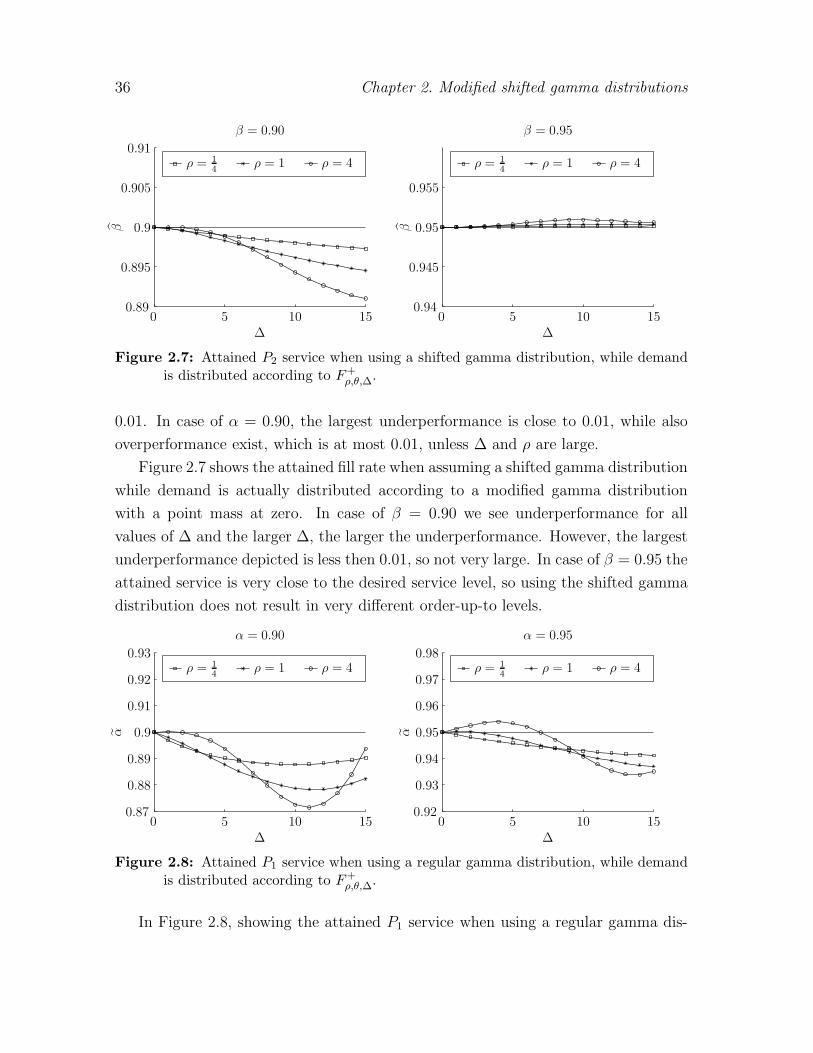
36 Chapter 2. Modified shifted gamma distributions
∆
ββ = 0.90
ρ = 14
ρ = 1 ρ = 4
0 5 10 150.89
0.895
0.9
0.905
0.91
∆
β
β = 0.95
ρ = 14
ρ = 1 ρ = 4
0 5 10 150.94
0.945
0.95
0.955
Figure 2.7: Attained P2 service when using a shifted gamma distribution, while demandis distributed according to F+
ρ,θ,∆.
0.01. In case of α = 0.90, the largest underperformance is close to 0.01, while also
overperformance exist, which is at most 0.01, unless ∆ and ρ are large.
Figure 2.7 shows the attained fill rate when assuming a shifted gamma distribution
while demand is actually distributed according to a modified gamma distribution
with a point mass at zero. In case of β = 0.90 we see underperformance for all
values of ∆ and the larger ∆, the larger the underperformance. However, the largest
underperformance depicted is less then 0.01, so not very large. In case of β = 0.95 the
attained service is very close to the desired service level, so using the shifted gamma
distribution does not result in very different order-up-to levels.
∆
α
α = 0.90
ρ = 14
ρ = 1 ρ = 4
0 5 10 150.87
0.88
0.89
0.9
0.91
0.92
0.93
∆
α
α = 0.95
ρ = 14
ρ = 1 ρ = 4
0 5 10 150.92
0.93
0.94
0.95
0.96
0.97
0.98
Figure 2.8: Attained P1 service when using a regular gamma distribution, while demandis distributed according to F+
ρ,θ,∆.
In Figure 2.8, showing the attained P1 service when using a regular gamma dis-

2.5. Mistakenly using the (shifted) gamma distribution 37
tribution, we see that when α = 0.90, the desired service is only reached for small
values of ∆; otherwise there exist underperformance, which is at most almost 0.03.
The underperformance first is getting bigger when ∆ is getting bigger, but it is de-
creasing after a certain point. In case of α = 0.95 the attained service levels show
approximately the same pattern; they are a little closer to the desired service levels
and in case of ρ = 4, we even see a small overperformance for relative small values
for ∆. The largest underperformance is almost 0.02 in this case.
∆
β
β = 0.90
ρ = 14
ρ = 1 ρ = 4
0 5 10 150.87
0.88
0.89
0.9
0.91
0.92
0.93
∆
β
β = 0.95
ρ = 14
ρ = 1 ρ = 4
0 5 10 150.92
0.93
0.94
0.95
0.96
0.97
0.98
Figure 2.9: Attained P2 service when using a regular gamma distribution, while demandis distributed according to F+
ρ,θ,∆.
Figure 2.9, finally, shows the attained fill rates when using a regular gamma
distribution while we should use the modified gamma distribution. The graphs for
β = 0.90 and β = 0.95 are quite similar. Both show overperformance, being at most
a little over 0.02.
In general the under- and overperformance is not large. Therefore, it seems not
to lead to big problems when using the wrong distribution. However, also a small
underperformance could lead to loss of clientele if it happens frequently. Overperfor-
mance, on the other side, means that too much inventory is kept. Even a relative
small reduction in inventory could lead to large savings, if we consider a company
with large amounts of SKUs. Furthermore, the attained service level is closer to
the desired one if we consider a shifted gamma distribution compared to a regular
gamma distribution. This can be explained by the fact that the modified shifted
gamma distributions are closer to the shifted gamma distribution than to the regular
gamma distribution.

38 Chapter 2. Modified shifted gamma distributions
2.5.2 Not using F ∗
ρ,θ,∆
If we know that demand is distributed according to the shifted gamma distribution
truncated at zero with parameters ρ, θ and ∆, the first three moments are (see Section
2.3.2)
µ∗ =µ+
P , µ∗2 =
µ+2
P , and µ∗3 =
µ+3
P ,
where P = 1 − Fρ,θ,∆(0). Using these moments and the functions (2.10)–(2.12), we
can obtain estimates for the parameters of the shifted gamma distribution, denoted
by ρ∗, θ∗ and ∆∗. The order-up-to levels using the shifted gamma distribution, while
the true distribution is the truncated shifted gamma distribution, are
S∗α = F−1
ρ∗,θ∗,∆∗(α),
S∗β = G−1
ρ∗,θ∗,∆∗((1− β)µ∗),
for the cycle service and the fill rate service respectively. The attained service, α∗ and
β∗ is determined using that demand is truly truncated shifted gamma distributed:
α∗ = F ∗ρ,θ,∆(S
∗α),
β∗ = 1−1PGρ,θ,∆(S
∗β)
µ∗ .
Figures 2.10 and 2.11 show the attained service when a shifted gamma distribution is
used, while the demand is actually truncated shifted gamma distributed for different
values of ρ and ∆. The parameter θ is chosen according to 10ρ. Figure 2.10 shows the
attained P1 service for α = 0.90 and α = 0.95. The left and right graph are quite
similar, with under- and overperformance both occurring and both being small, i.e.,
less then 0.005. Note that in case of ρ = 1 the desired service level is reached exactly
for all values of ∆.
Figure 2.11 shows the attained fill rates. The graphs are actually quite similar
to the graphs in Figure 2.10; the main difference is that the attained service is even
closer to the desired service in case of β = 0.95. We can see that also in these graphs
the desired service is exactly reached in case of ρ = 1.
Note that the over- and underperformance is not bigger than 0.005, hence using
the shifted gamma distribution while in fact we should be using the truncated shifted
gamma distribution does not result in big problems.
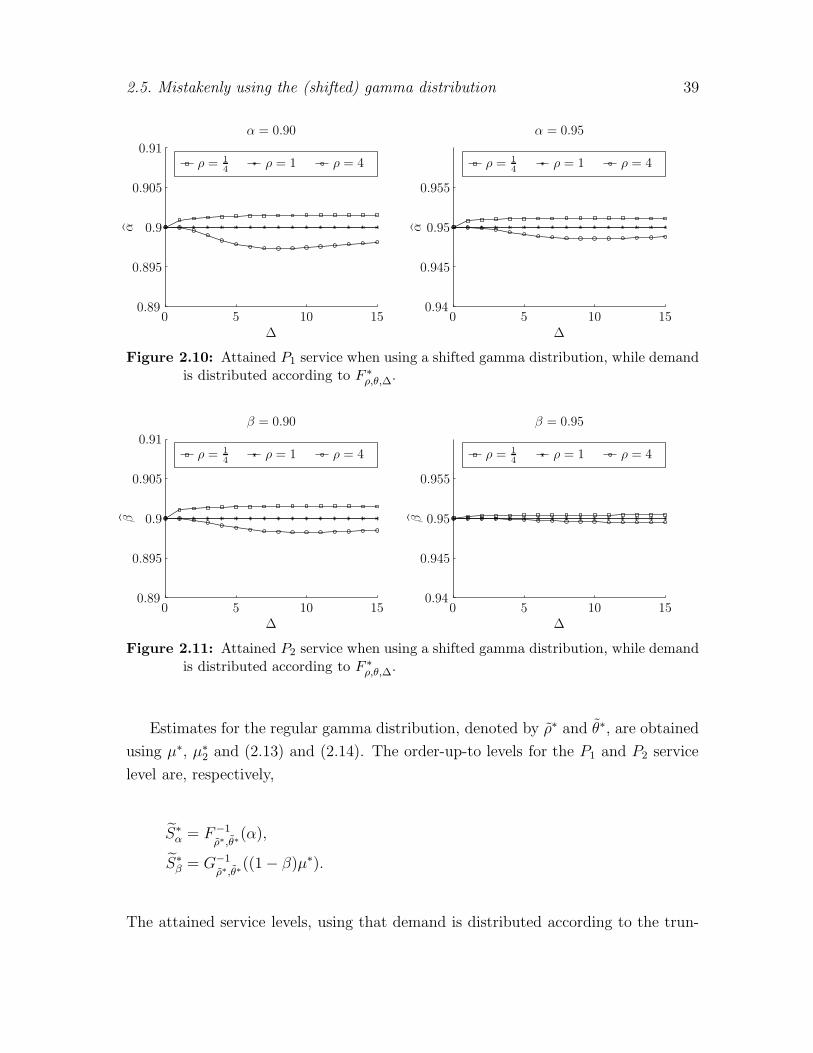
2.5. Mistakenly using the (shifted) gamma distribution 39
∆
αα = 0.90
ρ = 14
ρ = 1 ρ = 4
0 5 10 150.89
0.895
0.9
0.905
0.91
∆
α
α = 0.95
ρ = 14
ρ = 1 ρ = 4
0 5 10 150.94
0.945
0.95
0.955
Figure 2.10: Attained P1 service when using a shifted gamma distribution, while demandis distributed according to F ∗
ρ,θ,∆.
∆
β
β = 0.90
ρ = 14
ρ = 1 ρ = 4
0 5 10 150.89
0.895
0.9
0.905
0.91
∆
ββ = 0.95
ρ = 14
ρ = 1 ρ = 4
0 5 10 150.94
0.945
0.95
0.955
Figure 2.11: Attained P2 service when using a shifted gamma distribution, while demandis distributed according to F ∗
ρ,θ,∆.
Estimates for the regular gamma distribution, denoted by ρ∗ and θ∗, are obtained
using µ∗, µ∗2 and (2.13) and (2.14). The order-up-to levels for the P1 and P2 service
level are, respectively,
S∗α = F−1
ρ∗,θ∗(α),
S∗β = G−1
ρ∗,θ∗((1− β)µ∗).
The attained service levels, using that demand is distributed according to the trun-

40 Chapter 2. Modified shifted gamma distributions
cated shifted gamma distribution, are
α∗ = F ∗ρ,θ,∆(S
∗α),
β∗ = 1−1PGρ,θ,∆(S
∗β)
µ∗ .
Figures 2.12 and 2.13 show the attained service when the regular gamma distribu-
tion is used while demand is distributed according to the truncated modified shifted
gamma distribution for different values of ρ and ∆; θ is determined according to 10ρ.
Note that also in these figures the desired service level is exactly attained in case of
ρ = 1. Figure 2.12 show the attained cycle service for α = 0.90 and α = 0.95. The
∆
α
α = 0.90
ρ = 14
ρ = 1 ρ = 4
0 5 10 150.89
0.895
0.9
0.905
0.91
∆
α
α = 0.95
ρ = 14
ρ = 1 ρ = 4
0 5 10 150.94
0.945
0.95
0.955
Figure 2.12: Attained P1 service when using a regular gamma distribution, while demandis distributed according to F ∗
ρ,θ,∆.
left and right graph show both under- and overperformance, but the deviations from
the desired service level are small: all attained service levels are within 0.005 from
the desired service. Note that for α = 0.90 the deviations are a little larger compared
to the deviations when using the shifted gamma distribution, which is logical, since
the shifted gamma distribution is closer to the truncated shifted gamma distribution
compared to the regular gamma distribution.
Figure 2.13 show the attained P2 service for β = 0.90 and β = 0.95. The left
and right graph are quite similar: both show small underperformance in case of
ρ = 14and overperformance in case of ρ = 4. The deviations from the desired service
level are small: all attained service levels are within 0.005 from the desired service.
The deviations for both β = 0.90 and β = 0.95 are a little larger compared to the
deviations in 2.11; this is intuitively explained by the fact that the shifted gamma

2.6. Summary results 41
∆
ββ = 0.90
ρ = 14
ρ = 1 ρ = 4
0 5 10 150.89
0.895
0.9
0.905
0.91
∆
β
β = 0.95
ρ = 14
ρ = 1 ρ = 4
0 5 10 150.94
0.945
0.95
0.955
Figure 2.13: Attained P2 service when using a regular gamma distribution, while demandis distributed according to F ∗
ρ,θ,∆.
distribution is more similar to the truncated shifted gamma distribution than the
regular gamma distribution.
2.6 Summary results
This chapter discusses two modified shifted gamma distributions: one that has a
point mass at zero and one that is truncated at zero. These distributions provide
more flexible ways to model demand, at least when the lead time is zero, including
the possibility to model intermittent demand using one distribution instead of using
a compound distribution. The regular gamma distribution is a special case of both
modified shifted gamma distributions.
These two modified gamma distribution are used to model demand in a peri-
odic review, order-up-to level inventory control policy with zero lead time under two
service level restrictions. Using these distributions leads to nice expressions for the
order-up-to levels, hence, it is not very difficult to implement these distributions in
an inventory control system. Furthermore, we find that the order-up-to levels of the
shifted gamma distribution and the modified shifted gamma distribution with a point
mass at zero are equal when considering the cycle service. Besides that, the order-
up-to levels of the two modified shifted gamma distributions coincide when using the
fill rate service. Strijbosch and Moors (2006) found the same results for the normal
distribution and Section 2.4.3 shows that this holds for any modified distribution
with a point mass at zero and truncated modified distribution if they are constructed

42 Chapter 2. Modified shifted gamma distributions
in the same way as in this chapter.
Finally we show that using either the gamma distribution or the shifted gamma
distribution when demand is actually distributed according to one of the two modified
shifted gamma distributions leads to not reaching the desired service level (unless we
consider the truncated shifted gamma distribution and ρ = 1). The figures in Section
2.5 show that both under- and overperformance occur and that the attained service
is close to the desired one: the largest deviation from the desired service level is
0.03. However, even this small underperformance could have negative effects. If
one would have negotiated a certain service and in the long run this service is not
reached, customers could choose another supplier. Also, overperformance has its
disadvantages, since this implies that too much inventory is kept. Less inventory
would results in less inventory costs and even a relative little decrease could already
lead to large cost savings, as in many companies inventory costs are a substantial
part of the costs.
If these distributions are used in a real life inventory control policy, we need to
estimate the three parameters ρ, θ and ∆. We could use the expressions of the
first three moments of the modified demand distributions to estimate the demand
parameters. Of course, the true values of the first three moments are not known,
hence, we need to substitute the first, second and third moment by estimates of these
three moments. These estimates are obtained using historical demand observations.
Another possibility for finding estimates of the three demand parameters, is using
maximum likelihood estimators. Note that using estimators for the demand param-
eters will lead to randomness in the order-up-to level, as estimators themselves are
random variables and the order-up-to level is a function of the estimators. This will
probably lead to underperformance, that can be serious, as is shown in Chapters
3–5 for normally distributed demand, gamma distributed demand, and mixed Erlang
distributed demand, respectively.

Part II
Unknown demand parameters


Chapter 3
Normal demand with unknowndemand parameters
Inventory models need information about the demand distribution. Inpractice, this information is not known with certainty and has to be es-timated with often relatively few historical demand observations. Usingthese estimates leads to underperformance. This chapter focuses on nor-mal distributed demand and an (R, S) inventory control policy, where theorder-up-to level satisfies a service equation. The cause and size of this un-derperformance are determined. Furthermore the formulae for the order-up-to levels are corrected analytically where possible and otherwise by useof simulation and linear regression. Simulation shows that these correc-tions improve the attained service. This chapter is based on Janssen et al.(2009).
3.1 Introduction
This chapter considers the assumption that demand is normally distributed; the nor-
mality assumption is often used both in research and in practice, see Zeng and Hayya
(1999). Furthermore, see Strijbosch and Moors (2006) for references to recent arti-
cles that involve the normal distribution. The assumption of normality is made
because it yields tractable results and it seems to give quite good approximations
when used on demand data with a low coefficient of variation (Silver et al., 1998
and Zipkin, 2000). However, the normal distribution has two major disadvantages:
it is symmetric and can take on negative values, while demand is nonnegative and
often skewed to the right. This may not impose serious problems if the coefficient of

46 Chapter 3. Normal demand with unknown demand parameters
variation is low (Zipkin, 2000) or if the demand during review/lead time consists of
many individual and independent demands (Silver et al., 1998). However, for high
values of the coefficient of variation, these disadvantages get more important; hence
Strijbosch and Moors (2006) suggest two simple modifications of the normal distri-
bution (see also Section 2.2). Tyworth and O’Neill (1997) and Lau and Lau (2003)
investigate the (non)robustness of using the normal approximation with a reorder-
point, order quantity inventory policy.
We assume that demand is truly normally distributed, but that the parameters
of the normal distribution (the mean and variance) are unknown. These parameters
are estimated using historical demand observations and the effect of estimating the
parameters is studied. Silver and Rahnama (1986, 1987) have considered the effect
of estimating parameters when using a reorder-point, order quantity inventory policy
with a cost criterion. They construct a function that determines the expected cost of
estimating the demand distribution rather than knowing it, and they conclude that
this function is not symmetrical: underestimating the demand causes larger costs
than overestimating. In the second article they propose a method that deliberately
biases the reorder point upwards.
This chapter focuses on two service level criteria within an (R, S) inventory policy
with zero lead time. The independent and identically distributed demands during
review periods have a normal distribution with mean µ and standard deviation σ,
which leads to a coefficient of variation ν = σ/µ. As mentioned before, the normal
distribution could lead to negative demand and in our model this is interpreted as
returned goods, so demand is actually net demand (demanded goods minus returned
goods). In addition the goods returned by customers can be sent back to the supplier,
thus the inventory level at the start of a review period always equals S. Furthermore,
demand during t+1 consecutive review periods is assumed to be stationary, and the
first t periodic review demands are used to estimate the mean and standard deviation
of the demand in review period t+1. The mean and standard deviation are estimated
by their sample statistics. We prefer using sample statistics instead of exponential
smoothing, since derivations are more tractable, while the conclusions are similar. In
forecasting, using sample statistics in order to obtain estimates is often referred to
as (simple) moving average.
Section 3.2 discusses the P1 service criterion in short. An analytical correction
of the order-up-to level is given for the case that only µ is unknown. Section 3.3
focuses on the P2 service criterion. First two theoretical situations are considered for

3.2. P1 service level criterion 47
illustrative purposes: the case that µ is unknown, but σ and ν are known, and the
case that µ and σ are unknown, but ν is known. The main Sections 3.3.3 and 3.3.4
treat the important case that these three parameters are all unknown. We show by
simulation that just plugging in estimates leads to serious underperformance. Besides,
we develop a correction function for the safety factor that nearly gives the desired fill
rates. The last section provides a short summary of the results.
3.2 P1 service level criterion
This section considers the P1 service criterion. It is common to express the order-up-
to level as a function of the mean µ, the standard deviation σ, and a safety factor cα.
Since demand is normally distributed, the order-up-to level is (see, e.g., Silver et al.,
1998)
S(µ, σ, cα) = µ+ cασ. (3.1)
The safety factor cα is Φ−1(α), where Φ(·) is the cdf of the standard normal distribu-
tion. S without arguments is used to denote the theoretically correct order-up-to level
when all parameters are known, so S = S(µ, σ, cα) in case of a P1 service criterion.
In practice, the mean and variance are unknown, which means that S is unknown
too. The common solution is to replace the parameters µ and σ by its estimates. If
we (unrealistically) assume that only µ is unknown and use the sample mean dt to
estimate it, the resulting order-up-to level is S(dt, σ, cα) with dt =1t
∑ti=1 di, where
di is the observed demand during period i and t is the number of historical demand
observations. This order-up-to level, although unbiased, does not meet the service
requirements in the long run. Consider Figure 3.1. Since S(dt, σ, cα) is normally
distributed, with mean S and variance σ2/t, it is symmetric and the realization S − ε
is equally likely as the realization S+ε. The realization S+ε decreases the probability
of having backlogged demand with the darker area in Figure 3.1, while the realization
S − ε increases the probability of having backlogged demand with the lighter area.
The surface of the lighter area is larger than the surface of the darker area and this
implies that in the long run the achieved service level falls short of the desired one.
This phenomenon is mathematically explained by (τ denotes√1 + 1/t)
P(DR < S(dt, σ, cα)
)= P
(DR − dt < cασ
)= Φ
(cατ
)< Φ (cα) = α, (3.2)

48 Chapter 3. Normal demand with unknown demand parameters
if cα > 0, hence α > 0.5. Note that α > 0.50 is not a limitation in practice: in real
life the desired service level will be larger than 0.50.
µ S
S(dt, σ, cα)
DR
S − ε S + ε
Figure 3.1: The PDF of demand during review DR and order-up-to level S(dt, σ, cα).
Now let Z be a general biased estimator of S and let Z ∼ N(S + vσ, (w2 − 1)σ2),
where w ≥ 1. The probability of not having backorders in a review period is given
by
P (DR < Z) = Φ
(cα + v
w
). (3.3)
In general, this expression does not equal α, unless v and w are chosen according
to the relation v = (w − 1)cα (see also Strijbosch et al., 1997). This phenomenon is
depicted in Figure 3.2. The curved surface depicts the attained service level at values
of 0 ≤ v ≤ 1.6 and 1 ≤ w ≤ 1.5. The fine grid depicts the desired service level.
The attained service is below this level in some cases, while it is above it in other
cases. The attained service reaches the required one only on the solid line, for which
obviously holds v = (w− 1)cα. Furthermore, if an unbiased estimator is used (v = 0,
the dashed line), the desired service is reached only if w = 1. That case corresponds
to having an estimator with standard deviation equal to 0, which is not possible in
practice. So, an unbiased normally distributed estimator leads to underperformance.
Now consider the order-up-to level S(dt, στ, cα), where τ denotes√
1 + 1/t. This
order-up-to level is normally distributed with mean µ+ cαστ and variance σ2/t, so it
is a special case of Z with w = τ and v = (w − 1)cα; note that w cannot be chosen
freely, since the variance of the order-up-to level depends on the used estimator.
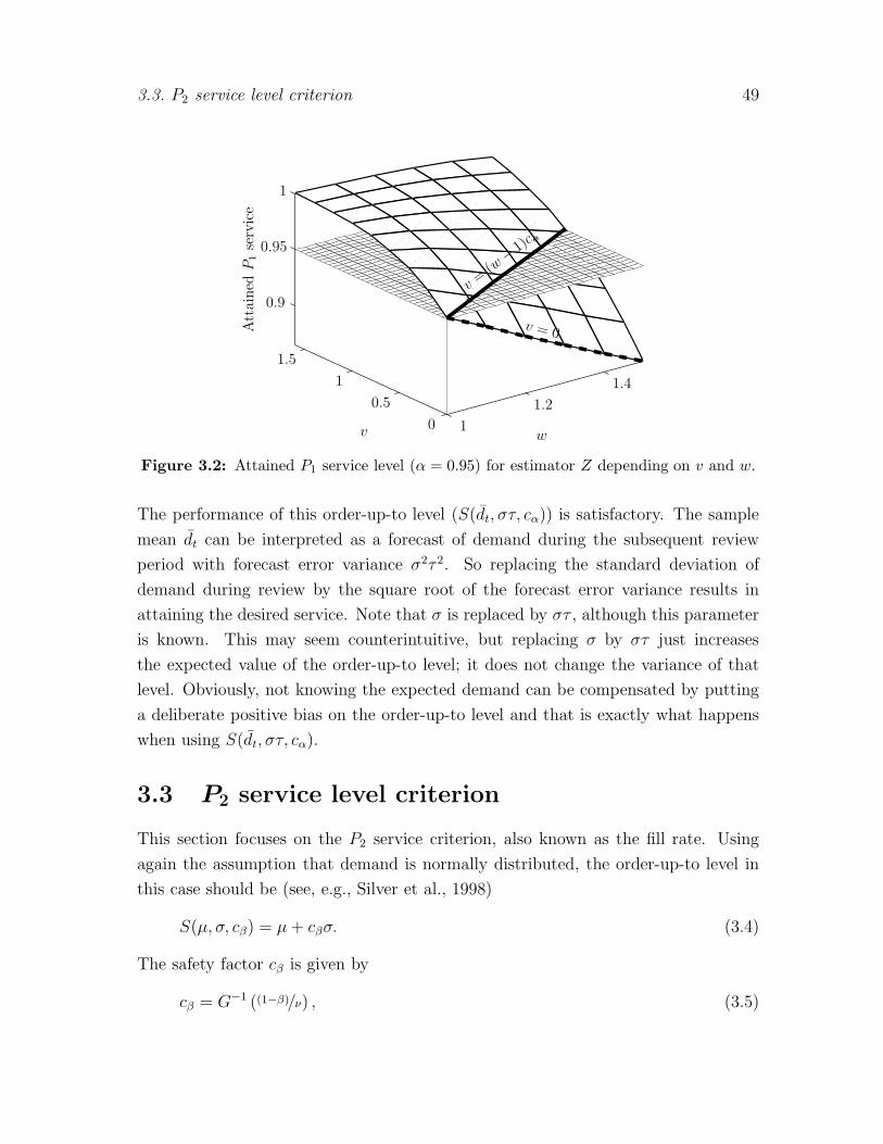
3.3. P2 service level criterion 49
v = 0
v =(w
− 1)cα
wv
Attained
P1service
1
1.2
1.4
0
0.5
1
1.5
0.9
0.95
1
Figure 3.2: Attained P1 service level (α = 0.95) for estimator Z depending on v and w.
The performance of this order-up-to level (S(dt, στ, cα)) is satisfactory. The sample
mean dt can be interpreted as a forecast of demand during the subsequent review
period with forecast error variance σ2τ 2. So replacing the standard deviation of
demand during review by the square root of the forecast error variance results in
attaining the desired service. Note that σ is replaced by στ , although this parameter
is known. This may seem counterintuitive, but replacing σ by στ just increases
the expected value of the order-up-to level; it does not change the variance of that
level. Obviously, not knowing the expected demand can be compensated by putting
a deliberate positive bias on the order-up-to level and that is exactly what happens
when using S(dt, στ, cα).
3.3 P2 service level criterion
This section focuses on the P2 service criterion, also known as the fill rate. Using
again the assumption that demand is normally distributed, the order-up-to level in
this case should be (see, e.g., Silver et al., 1998)
S(µ, σ, cβ) = µ+ cβσ. (3.4)
The safety factor cβ is given by
cβ = G−1 ((1−β)/ν) , (3.5)

50 Chapter 3. Normal demand with unknown demand parameters
where G (·) denotes the loss function of the standard normal distribution (G (x) =
E [(Y − x)+] with Y a standard normal random variable). Note that G (x) is equal
to G (x) = ϕ(x) − xΦ(−x), where ϕ(·) denotes the pdf of the standard normal
distribution. As in the previous section, S without arguments denotes the correct
order-up-to level. Furthermore, the service level attained by using an order-up-to
level Z is
1− E[(DR − Z)+
]
E [DR]= 1− E
[(DR − Z)+
]
µ. (3.6)
Note that if Z is constructed using estimates instead of the true values of the mean,
standard deviation and coefficient of variation, it is a random variable. When using a
P2 service criterion, one needs values of µ and σ, and, in contrast to the P1 criterion,
also the coefficient of variation ν plays a role, as can be seen from (3.5). In practice,
these parameters have to be estimated. The next two sections illustrate the effect of
estimating µ and σ in the case where the correct safety factor is used, i.e., when ν
is known. Section 3.3.3 considers the more realistic case where also the coefficient of
variation needs to be estimated, and hence the safety factor as well.
3.3.1 Only expected demand unknown
This section assumes that only µ is unknown and thus that σ and ν are known.
This is a purely theoretical assumption, since if σ and ν are known, µ can easily be
determined. Yet, this case is interesting since even now the commonly used order-
up-to level does not guarantee reaching the desired service level. If the sample mean
is used to estimate µ, the order-up-to level is S(dt, σ, cβ). Note that S(dt, σ, cβ) is
normally distributed with mean S and variance σ2/t. Using S(dt, σ, cβ) does not result
in attaining the desired service level β in the long run:
1−E
[(DR − S(dt, σ, cβ)
)+]
µ= 1− στG
( cβτ
)
µ< 1− ντG (cβ)
= 1− ντ1− β
ν< β, (3.7)
where τ still denotes√
1 + 1/t. The first inequality follows from the fact that the
derivative of G (x) is −Φ(−x) < 0, so G (x) is a strictly decreasing function. Note
also that cβ has to be positive, or, β > 1 − ν/√2π. Again, this is not a limitation in
practice, since the desired service level will be high. Only if ν <√
π/50 ≈ 0.2507 the

3.3. P2 service level criterion 51
desired service level needs to be larger than 0.90 for the first inequality in (3.7) to
hold.
Again, even in this simple case, using the unbiased estimator for S leads to a
lower attained service level than β. We consider both the attained service levels (β)
and their relative deviations (δβ(β)). The relative deviation δβ(β) is defined as
δβ(β) =(1− β)− (1− β)
(1− β)=
β − β
1− β,
where β is the attained service level and β the desired service level. This is a good
performance measure, since it takes the height of the desired service level into account:
if the service is 0.01 too low when the desired service level is 0.90, it will not be
considered as bad as when the desired service level is 0.99. Note that when δβ(β) is
positive, β is less than β and we experience underperformance; when δβ(β) < 0, there
is overperformance. Overperformance might not be as bad as underperformance, but
it implies that too many items are in inventory and we could reach the desired service
level with less inventory, hence with less costs. Five different attained service levels
and their relative deviations are discussed in the remainder of this chapter; these
attained service levels and there notation is listed in Table 3.1.
β0: Attained service when µ unknown, but σ and ν known (Section 3.3.1);
β1: Attained service when µ and σ unknown, but ν known (Section 3.3.2);
β2: Attained service when µ, σ, and ν unknown (Section 3.3.3);
β3: Attained service when using correction function κσ(ν, t, β) (Section 3.3.4);
β4: Attained service when using correction function κs(ν, t, β) (Section 3.3.4).
Table 3.1: The attained service levels discussed in Section 3.3 and their notation.
The attained service and its relative deviation assuming that only µ is unknown
are shown in Figure 3.3; note that the x- and y-axes in the right graphs are reversed
compared to the left graphs. This figure shows that the underperformance is larger
when t is smaller (ceteris paribus, c.p. for short), when ν is larger (c.p.) and when β is
larger (c.p.; underperformance measured through δβ(β0)). When t is smaller, the vari-
ance of the order-up-to level is larger, hence, intuitively the underperformance should
be larger too. The same line of reasoning applies to ν being larger; also in that case the
variance of the order-up-to level is larger and thus the underperformance is larger. If

52 Chapter 3. Normal demand with unknown demand parameters
ν t
β0
β = 0.90
0.2
0.5
0.8 26
1015
0.8
0.85
0.9
ν t
δ β(β
0)
β = 0.90
0.2
0.5
0.82
610
15
0
0.5
1
ν t
β0
β = 0.95
0.2
0.5
0.8 26
1015
0.85
0.9
0.95
ν t
δ β(β
0)
β = 0.95
0.2
0.5
0.82
610
15
0
1
2
ν t
β0
β = 0.99
0.2
0.5
0.8 26
1015
0.9
0.95
1
ν t
δ β(β
0)
β = 0.99
0.2
0.5
0.82
610
15
0
5
10
Figure 3.3: Attained service (β0) and relative deviation (δβ(β0)) if only µ unknown.
β is larger, 1 − β is smaller and the same absolute deviation is worse if β is larger,
hence the underperformance, measured through the relative deviation, is larger. The
extreme attained service levels for all three desired service levels are displayed in
Table 3.2. One can clearly see that the deviations from the desired service level
cannot be neglected, since they can become as large as 0.0561 (0.90− 0.8439), which

3.3. P2 service level criterion 53
Desired service Minimum attained Maximum attained Mean attained
level service (δβ(β0)) service (δβ(β0)) service (δβ(β0))β = 0.90 0.8439 (0.561) 0.8974 (0.026) 0.8838 (0.162)β = 0.95 0.9080 (0.840) 0.9475 (0.050) 0.9372 (0.256)β = 0.99 0.9721 (1.790) 0.9888 (0.120) 0.9844 (0.560)
Table 3.2: Extreme deviations for β ∈ {0.90, 0.95, 0.99} when only µ unknown.
is more than 5 percent points below the desired service.
In case of the P1 criterion, the problem of underperformance was solved by re-
placing the standard deviation σ by the square root of the forecast error variance,
στ . So we might apply the same adjustment in this case. Note however that σ has to
be replaced twice: once explicitly and once implicitly, as the safety factor cβ depends
on σ via ν. Now let us denote the new safety factor by cτβ:
cτβ = G−1
(1− β
ντ
). (3.8)
Obviously cτβ > cβ. Upwards biasing the safety factor has been mentioned in the
literature; see Section 3.1. However, to our knowledge, applying the factor τ both
to the explicit and the implicit standard deviation has never been mentioned. Now
consider the attained service level when using the order-up-to level S(dt, στ, cτβ):
1−E
[(DR − S(dt, στ, c
τβ))+]
µ= 1− ντG
(cτβ)= 1− ντ
1− β
ντ= β. (3.9)
So using S(dt, στ, cτβ) indeed results in attaining the desired service level in the long
run.
3.3.2 Expected demand and its variance unknown (ν known)
Now assume that only ν is known, so σ has to be estimated too. We choose to use
the sample standard deviation st. One could also use the known ν and the estimate
of µ to estimate the value of σ, but since the next step is to assume that ν is also
unknown, we do not follow that approach. The sample standard deviation is defined
as st =√
1t−1
∑ti=1
(di − dt
)2. Substituting this estimator yields the order-up-to level
S(dt, stτ, cτβ). Consider the expected value of this order-up-to level and note that s2t
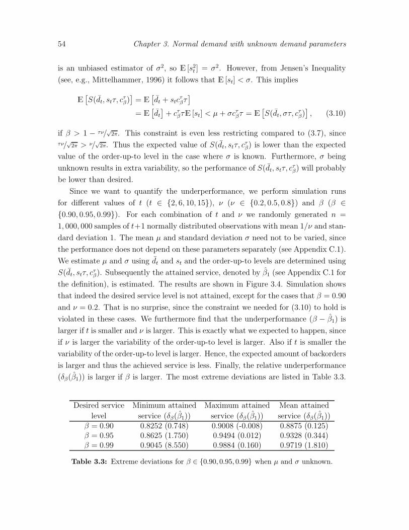
54 Chapter 3. Normal demand with unknown demand parameters
is an unbiased estimator of σ2, so E [s2t ] = σ2. However, from Jensen’s Inequality
(see, e.g., Mittelhammer, 1996) it follows that E [st] < σ. This implies
E[S(dt, stτ, c
τβ)]= E
[dt + stc
τβτ]
= E[dt]+ cτβτE [st] < µ+ σcτβτ = E
[S(dt, στ, c
τβ)], (3.10)
if β > 1 − τν/√2π. This constraint is even less restricting compared to (3.7), since
τν/√2π > ν/
√2π. Thus the expected value of S(dt, stτ, c
τβ) is lower than the expected
value of the order-up-to level in the case where σ is known. Furthermore, σ being
unknown results in extra variability, so the performance of S(dt, stτ, cτβ) will probably
be lower than desired.
Since we want to quantify the underperformance, we perform simulation runs
for different values of t (t ∈ {2, 6, 10, 15}), ν (ν ∈ {0.2, 0.5, 0.8}) and β (β ∈{0.90, 0.95, 0.99}). For each combination of t and ν we randomly generated n =
1, 000, 000 samples of t+1 normally distributed observations with mean 1/ν and stan-
dard deviation 1. The mean µ and standard deviation σ need not to be varied, since
the performance does not depend on these parameters separately (see Appendix C.1).
We estimate µ and σ using dt and st and the order-up-to levels are determined using
S(dt, stτ, cτβ). Subsequently the attained service, denoted by β1 (see Appendix C.1 for
the definition), is estimated. The results are shown in Figure 3.4. Simulation shows
that indeed the desired service level is not attained, except for the cases that β = 0.90
and ν = 0.2. That is no surprise, since the constraint we needed for (3.10) to hold is
violated in these cases. We furthermore find that the underperformance (β − β1) is
larger if t is smaller and ν is larger. This is exactly what we expected to happen, since
if ν is larger the variability of the order-up-to level is larger. Also if t is smaller the
variability of the order-up-to level is larger. Hence, the expected amount of backorders
is larger and thus the achieved service is less. Finally, the relative underperformance
(δβ(β1)) is larger if β is larger. The most extreme deviations are listed in Table 3.3.
Desired service Minimum attained Maximum attained Mean attained
level service (δβ(β1)) service (δβ(β1)) service (δβ(β1))β = 0.90 0.8252 (0.748) 0.9008 (-0.008) 0.8875 (0.125)β = 0.95 0.8625 (1.750) 0.9494 (0.012) 0.9328 (0.344)β = 0.99 0.9045 (8.550) 0.9884 (0.160) 0.9719 (1.810)
Table 3.3: Extreme deviations for β ∈ {0.90, 0.95, 0.99} when µ and σ unknown.

3.3. P2 service level criterion 55
ν t
β1
β = 0.90
0.2
0.5
0.8 26
1015
0.8
0.85
0.9
ν t
δ β(β
1)
β = 0.90
0.2
0.5
0.82
610
15
0
0.5
1
ν t
β1
β = 0.95
0.2
0.5
0.8 26
1015
0.85
0.9
0.95
ν t
δ β(β
1)
β = 0.95
0.2
0.5
0.82
610
15
0
1
2
ν t
β1
β = 0.99
0.2
0.5
0.8 26
1015
0.9
0.95
1
ν t
δ β(β
1)
β = 0.99
0.2
0.5
0.82
610
15
0
5
10
Figure 3.4: Attained service (β1) and relative deviation (δβ(β1)) if µ and σ unknown.
Since it is difficult to consider this case analytically and it is not of practical
interest (as ν is assumed to be known), we continue with the most practical case, in
which all parameters are unknown.
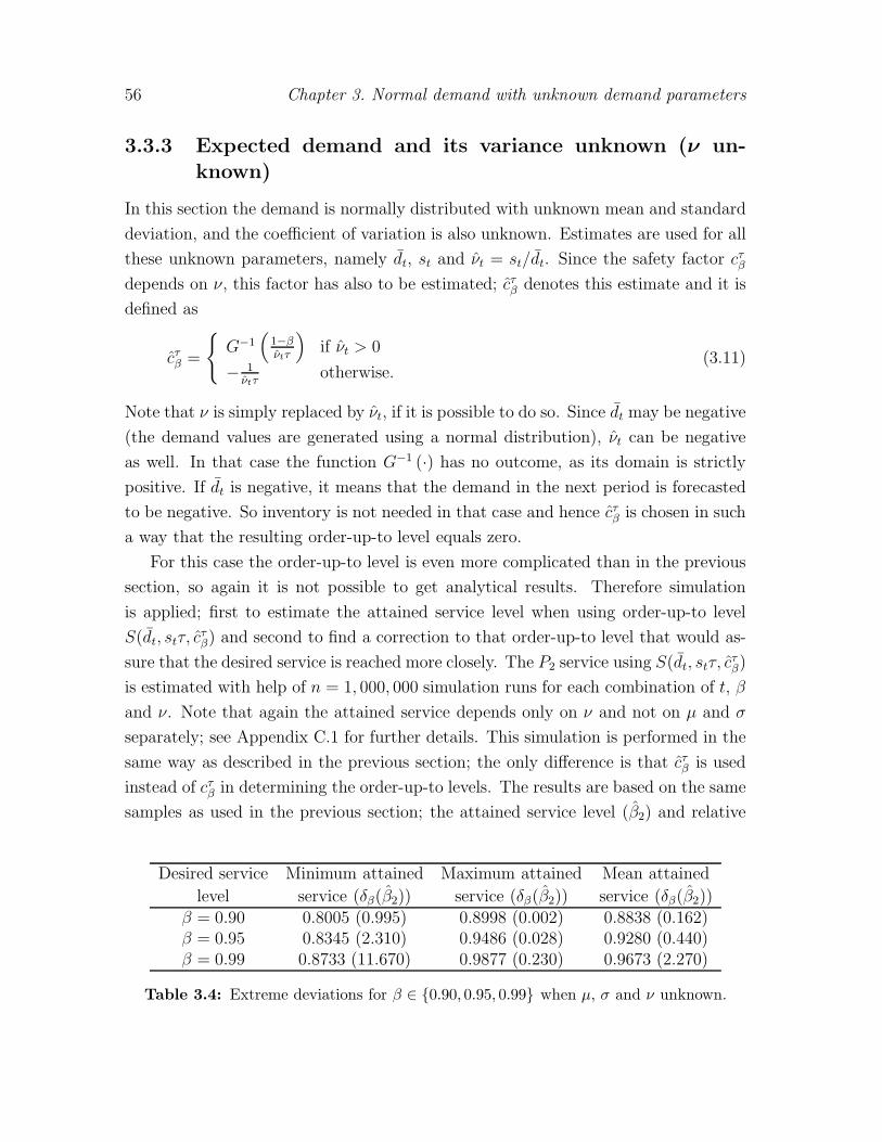
56 Chapter 3. Normal demand with unknown demand parameters
3.3.3 Expected demand and its variance unknown (ν un-
known)
In this section the demand is normally distributed with unknown mean and standard
deviation, and the coefficient of variation is also unknown. Estimates are used for all
these unknown parameters, namely dt, st and νt = st/dt. Since the safety factor cτβdepends on ν, this factor has also to be estimated; cτβ denotes this estimate and it is
defined as
cτβ =
{G−1
(1−βνtτ
)if νt > 0
− 1νtτ
otherwise.(3.11)
Note that ν is simply replaced by νt, if it is possible to do so. Since dt may be negative
(the demand values are generated using a normal distribution), νt can be negative
as well. In that case the function G−1 (·) has no outcome, as its domain is strictly
positive. If dt is negative, it means that the demand in the next period is forecasted
to be negative. So inventory is not needed in that case and hence cτβ is chosen in such
a way that the resulting order-up-to level equals zero.
For this case the order-up-to level is even more complicated than in the previous
section, so again it is not possible to get analytical results. Therefore simulation
is applied; first to estimate the attained service level when using order-up-to level
S(dt, stτ, cτβ) and second to find a correction to that order-up-to level that would as-
sure that the desired service is reached more closely. The P2 service using S(dt, stτ, cτβ)
is estimated with help of n = 1, 000, 000 simulation runs for each combination of t, β
and ν. Note that again the attained service depends only on ν and not on µ and σ
separately; see Appendix C.1 for further details. This simulation is performed in the
same way as described in the previous section; the only difference is that cτβ is used
instead of cτβ in determining the order-up-to levels. The results are based on the same
samples as used in the previous section; the attained service level (β2) and relative
Desired service Minimum attained Maximum attained Mean attained
level service (δβ(β2)) service (δβ(β2)) service (δβ(β2))β = 0.90 0.8005 (0.995) 0.8998 (0.002) 0.8838 (0.162)β = 0.95 0.8345 (2.310) 0.9486 (0.028) 0.9280 (0.440)β = 0.99 0.8733 (11.670) 0.9877 (0.230) 0.9673 (2.270)
Table 3.4: Extreme deviations for β ∈ {0.90, 0.95, 0.99} when µ, σ and ν unknown.
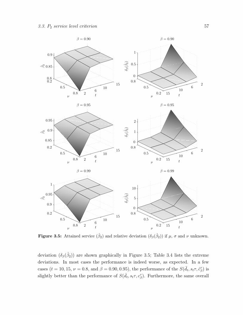
3.3. P2 service level criterion 57
ν t
β2
β = 0.90
0.2
0.5
0.8 26
1015
0.8
0.85
0.9
ν t
δ β(β
2)
β = 0.90
0.2
0.5
0.82
610
15
0
0.5
1
ν t
β2
β = 0.95
0.2
0.5
0.8 26
1015
0.85
0.9
0.95
ν t
δ β(β
2)
β = 0.95
0.2
0.5
0.82
610
15
0
1
2
ν t
β2
β = 0.99
0.2
0.5
0.8 26
1015
0.9
0.95
1
ν t
δ β(β
2)
β = 0.99
0.2
0.5
0.82
610
15
0
5
10
Figure 3.5: Attained service (β2) and relative deviation (δβ(β2)) if µ, σ and ν unknown.
deviation (δβ(β2)) are shown graphically in Figure 3.5; Table 3.4 lists the extreme
deviations. In most cases the performance is indeed worse, as expected. In a few
cases (t = 10, 15, ν = 0.8, and β = 0.90, 0.95), the performance of the S(dt, stτ, cτβ) is
slightly better than the performance of S(dt, stτ, cτβ). Furthermore, the same overall

58 Chapter 3. Normal demand with unknown demand parameters
results as in Section 3.3.2 appear: the underperformance increases as t decreases and
as ν increases. The relative underperformance also increases as β increases.
3.3.4 Correction of the order-up-to level
Now the underperformance is quantified in Section 3.3.3, we also want to find a cor-
rection for S(dt, stτ, cτβ), such that the desired service is reached or at least approached
more closely. This correction depends on ν, t and β and is denoted by κ (ν, t, β). Such
a correction function can be useful in practice, since it provides inventory managers
with a simple tool to improve their easy-to-understand order-up-to levels. After con-
sidering several options to correct the order-up-to level, a dimensionless correction
factor is determined in order to provide an upwards bias to S(dt, stτ, cτβ). The cor-
rected order-up-to level is S(dt+κ (ν, t, β) st, stτ, cτβ). Note that this is not applicable
in practice, since ν is unknown. However, replacing ν by νt does improve the attained
service, as is shown in Figures 3.8 and 3.9.
Simulation is used to estimate the correction needed for various values of ν, t and
β. The two simulations performed earlier used only a limited number of values for
the three parameters; more values are needed to be able to estimate the correction
using ν, t, and β. So a new simulation is performed in which n = 100, 000 samples of
t + 1 observations are generated for each combination of t, ν, and β; (3.12) provides
the values of the three parameters used in the simulation:
T = {2, 3, 4, 5, 6, 7, 8, 10, 12, 15, 20}V = {0.1, 0.2, 0.3, 0.4, 0.5, 0.6, 0.7, 0.8, 0.9, 1.0}B = {0.90, 0.91, 0.92, 0.93, 0.94, 0.95, 0.96, 0.97, 0.98, 0.99}.
(3.12)
The range of the values do not differ much from the range used in the earlier simula-
tions (t between 2 and 15; ν between 0.2 and 0.8; β between 0.90 and 0.99). The size
of the underperformance will not become much larger; only when ν = 0.9 and ν = 1
and t small the differences are larger than the values reported in Tables 3.2–3.4.
The number of generated samples is smaller, since we need considerably more
simulations, which are time-consuming; the complete simulation needed more than
one week to finish. For each simulation run j (j = 1, . . . , n) the estimated order-
up-to level, denoted by Sj, is calculated using the first t observations and the (t +
1)th observation dj is used to quantify the backlogged demand that occurred. The
correction needed can be determined using either the true value σ or the sample

3.3. P2 service level criterion 59
standard deviations stj (j = 1, . . . , n) found in the simulation. On the one hand
using the true value might be better, since it is the true value. On the other hand, a
correction is needed since an estimate is used instead of the true value. It is difficult to
decide a priori which would result in a better correction formula, so both corrections,
denoted by kσ and ks respectively, are determined, by solving the following two
equations:
n∑
j=1
(dj − (Sj + kσσ))+ = (1− β)
n∑
j=1
dj, (3.13)
n∑
j=1
(dj − (Sj + ksstj))+ = (1− β)
n∑
j=1
dj. (3.14)
The values for kσ and ks for all combinations of ν, t and β can be found by solving
this equation numerically using binary search. Note that the left hand sides of (3.13)
and (3.14) are decreasing in kσ and ks, so there is one value for kσ and one for ks
for which equality holds. The corrections are denoted by ki (ν, t, β) (i ∈ {σ, s}). Thecorrections for different values of ν, t and β are depicted in Figures 3.6 and 3.7.
ν t
kσ(ν,t,β
)
Average over β = 0.90–0.93
0.5
1510
1520
0
0.5
1
1.5
ν t
kσ(ν,t,β
)
Average over β = 0.94–0.96
0.5
1510
1520
0
0.5
1
1.5
ν t
kσ(ν,t,β
)
Average over β = 0.97–0.98
0.5
15
1015
20
0
0.5
1
1.5
ν t
kσ(ν,t,β
)
β = 0.99
0.5
15
1015
20
0
0.5
1
1.5
Figure 3.6: Corrections kσ (ν, t, β) of the order-up-to level S(dt, stτ, cτβ).

60 Chapter 3. Normal demand with unknown demand parameters
ν t
ks(ν,t,β
)
Average over β = 0.90–0.93
0.5
1510
1520
0
10
20
ν t
ks(ν,t,β
)
Average over β = 0.94–0.96
0.5
1510
1520
0
10
20
ν t
ks(ν,t,β
)
Average over β = 0.97–0.98
0.5
15
101520
0
10
20
ν t
ks(ν,t,β
)
β = 0.99
0.5
15
101520
0
10
20
Figure 3.7: Corrections ks (ν, t, β) of the order-up-to level S(dt, stτ, cτβ).
For the first three graphs in Figures 3.6 and 3.7 the corrections needed for different
values of β are averaged, since they do not differ much. One sees that if ν increases,
the correction needs to be larger. The same is true if t decreases and if β increases.
These conclusions correspond to the results in Section 3.3.3.
The simulation resulted in some values kσ (ν, t, β) and ks (ν, t, β), but a func-
tion that is able to estimate these values is more practical. Therefore a regression
technique we call nested regression is applied, following the method described by
Strijbosch and Moors (1999). This method is described elaborately in Appendix B.
The estimation process is split into three steps:
1. Choose one of the three parameters (denoted by q1), and use linear regres-
sion to estimate the correction needed depending on that parameter for each
combination of the other two parameters;
2. Choose one of the remaining two parameters (q2) and regress that parameter
on the coefficients found in Step 1 for each value of the third parameter;
3. Regress the third parameter (q3) on the coefficients found in Step 2.

3.3. P2 service level criterion 61
Finally the regression equations are combined in order to get a correction function.
A different ordering of choosing the parameters could influence the result, hence
all six orderings are examined, both for kσ (ν, t, β) and ks (ν, t, β). Example B.2 in
Appendix B shows how ks (ν, t, β) is constructed in detail. The fit, determined by R2
(coefficient of determination), of all possible orderings of adding the parameters and
for both kσ (ν, t, β) and ks (ν, t, β) are given in Table 3.5. So using ks (ν, t, β) instead
q1 q2 q3 R2 of kσ (ν, t, β) R2 of ks (ν, t, β)t ν β 0.9897 0.9960t β ν 0.9894 0.9962ν t β 0.9828 0.9963ν β t 0.9872 0.9889β t ν 0.9876 0.9958β ν t 0.9840 0.9900
Table 3.5: R2 found for different orderings of choosing parameters.
of kσ (ν, t, β) results in slightly better values of R2, although the R2s for both correc-
tions are very good. Next a simulation is performed to determine which correction
provides the best performance. Again the samples of size n = 1, 000, 000 are used
(see Section 3.3.2), now to determine the performance of S(dt+ κσ (νt, t, β) st, stτ, cτβ)
and S(dt + κs (νt, t, β) st, stτ, cτβ). The function κσ (νt, t, β) is based on kσ (ν, t, β) de-
termined using q1 = t, q2 = ν and q3 = β, while κs (νt, t, β) is based on ks (ν, t, β)
determined using q1 = ν, q2 = t and q3 = β; the corresponding R2s are printed in
boldface in Table 3.5. Also the performance of these order-up-to levels is independent
of σ and µ; see Appendix C.1.
Figure 3.8 shows the attained service levels (β3) and the corresponding relative
deviations (δβ(β3)) when using κσ (·). Table 3.6 lists the extreme deviations using
this correction function.
Desired service Minimum attained Maximum attained Mean attained
level service (δβ(β1)) service (δβ(β3)) service (δβ(β3))β = 0.90 0.8449 (0.551) 0.9005 (-0.005) 0.8917 (0.083)β = 0.95 0.8882 (1.236) 0.9497 (0.006) 0.9400 (0.200)β = 0.99 0.9332 (5.680) 0.9900 (0.000) 0.9796 (1.040)
Table 3.6: Extreme deviations for β ∈ {0.90, 0.95, 0.99} using correction κσ (νt, t, β).

62 Chapter 3. Normal demand with unknown demand parameters
ν t
β3
β = 0.90
0.2
0.5
0.8 26
1015
0.8
0.85
0.9
ν t
δ β(β
3)
β = 0.90
0.2
0.5
0.82
610
15
0
0.5
1
ν t
β3
β = 0.95
0.2
0.5
0.8 26
1015
0.85
0.9
0.95
ν t
δ β(β
3)
β = 0.95
0.2
0.5
0.82
610
15
0
1
2
ν t
β3
β = 0.99
0.2
0.5
0.8 26
1015
0.9
0.95
1
ν t
δ β(β
3)
β = 0.99
0.2
0.5
0.82
610
15
0
5
10
Figure 3.8: Attained service (β3) and relative deviation (δβ(β3)) using correctionκσ (νt, t, β).
The resulting attained service levels (β4) when using κs (·) are displayed in Fig-
ure 3.9, together with the relative deviations (δβ(β4)). The extreme deviations when
using the second correction function are shown in Table 3.7. Comparing the results

3.3. P2 service level criterion 63
ν t
β4
β = 0.90
0.2
0.5
0.8 26
1015
0.8
0.85
0.9
ν t
δ β(β
4)
β = 0.90
0.2
0.5
0.82
610
15
0
0.5
1
ν t
β4
β = 0.95
0.2
0.5
0.8 26
1015
0.85
0.9
0.95
ν t
δ β(β
4)
β = 0.95
0.2
0.5
0.82
610
15
0
1
2
ν t
β4
β = 0.99
0.2
0.5
0.8 26
1015
0.9
0.95
1
ν t
δ β(β
4)
β = 0.99
0.2
0.5
0.82
610
15
0
5
10
Figure 3.9: Attained service (β4) and relative deviation (δβ(β4)) using correctionκs (νt, t, β).
of using a correction, either κσ (·) or κs (·), to not using a correction, we see that the
achieved service level is closer to the desired one in most cases (33 out of 36 for κσ (·)and 28 out of 36 for κs (·)). So we may conclude that using a correction improves the
attained service level.
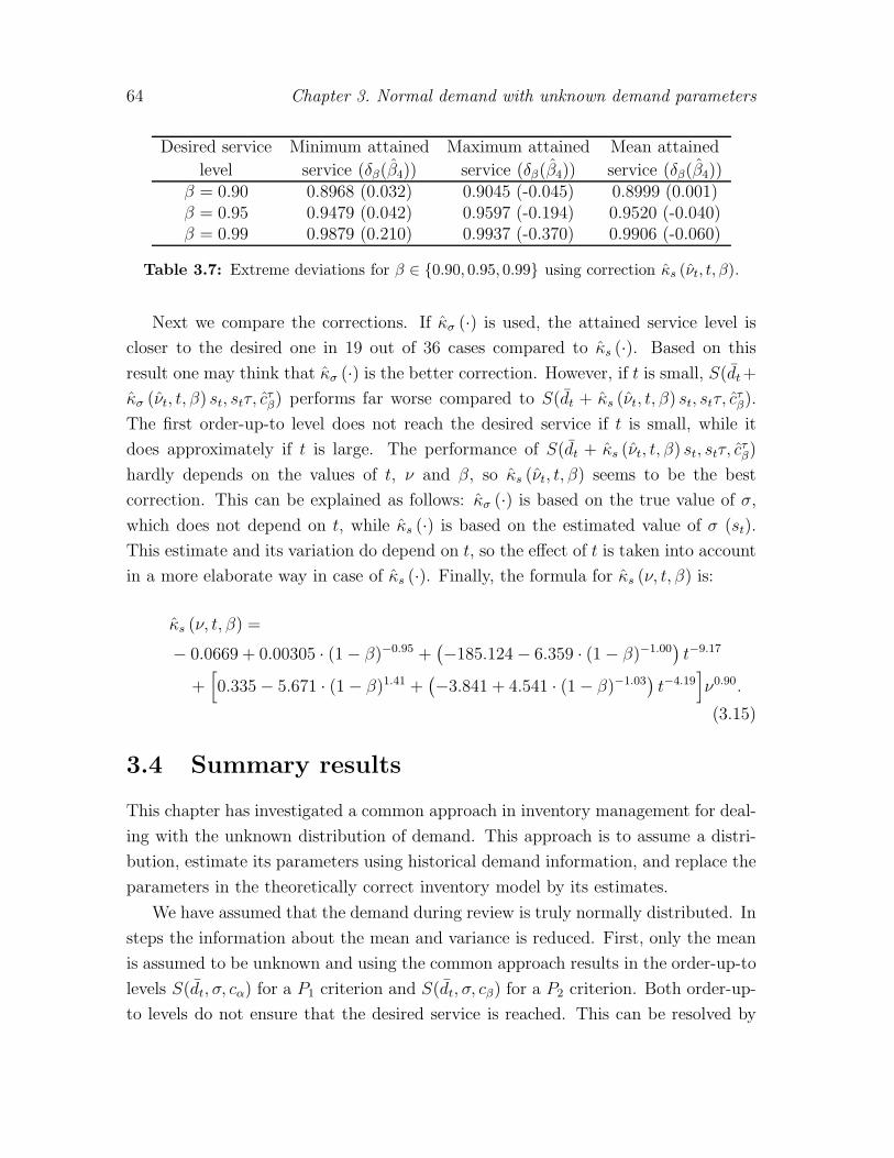
64 Chapter 3. Normal demand with unknown demand parameters
Desired service Minimum attained Maximum attained Mean attained
level service (δβ(β4)) service (δβ(β4)) service (δβ(β4))β = 0.90 0.8968 (0.032) 0.9045 (-0.045) 0.8999 (0.001)β = 0.95 0.9479 (0.042) 0.9597 (-0.194) 0.9520 (-0.040)β = 0.99 0.9879 (0.210) 0.9937 (-0.370) 0.9906 (-0.060)
Table 3.7: Extreme deviations for β ∈ {0.90, 0.95, 0.99} using correction κs (νt, t, β).
Next we compare the corrections. If κσ (·) is used, the attained service level is
closer to the desired one in 19 out of 36 cases compared to κs (·). Based on this
result one may think that κσ (·) is the better correction. However, if t is small, S(dt+
κσ (νt, t, β) st, stτ, cτβ) performs far worse compared to S(dt + κs (νt, t, β) st, stτ, c
τβ).
The first order-up-to level does not reach the desired service if t is small, while it
does approximately if t is large. The performance of S(dt + κs (νt, t, β) st, stτ, cτβ)
hardly depends on the values of t, ν and β, so κs (νt, t, β) seems to be the best
correction. This can be explained as follows: κσ (·) is based on the true value of σ,
which does not depend on t, while κs (·) is based on the estimated value of σ (st).
This estimate and its variation do depend on t, so the effect of t is taken into account
in a more elaborate way in case of κs (·). Finally, the formula for κs (ν, t, β) is:
κs (ν, t, β) =
− 0.0669 + 0.00305 · (1− β)−0.95 +(−185.124− 6.359 · (1− β)−1.00
)t−9.17
+[0.335− 5.671 · (1− β)1.41 +
(−3.841 + 4.541 · (1− β)−1.03
)t−4.19
]ν0.90.
(3.15)
3.4 Summary results
This chapter has investigated a common approach in inventory management for deal-
ing with the unknown distribution of demand. This approach is to assume a distri-
bution, estimate its parameters using historical demand information, and replace the
parameters in the theoretically correct inventory model by its estimates.
We have assumed that the demand during review is truly normally distributed. In
steps the information about the mean and variance is reduced. First, only the mean
is assumed to be unknown and using the common approach results in the order-up-to
levels S(dt, σ, cα) for a P1 criterion and S(dt, σ, cβ) for a P2 criterion. Both order-up-
to levels do not ensure that the desired service is reached. This can be resolved by

3.4. Summary results 65
replacing the standard deviation σ with the square root of the forecast error variance
στ , where τ =√
1 + 1/t.
Second, also the standard deviation becomes unknown, although the coefficient
of variation is assumed to be known. This case is less tractable and, therefore, only
the more interesting P2 criterion is considered for this case. The order-up-to level
using the correction factor τ becomes S(dt, stτ, cτβ), for which we have shown that the
expected value is too low. Furthermore, simulation has shown that the desired service
is indeed not reached when using this order-up-to level. Underperformance ranges
from 0.0875 to 0.0006 (in one case a small overperformance of 0.0008 is obtained);
the relative deviation ranges from 8.550 to −0.008).
Finally, also the coefficient of variation ν is unknown and in that case only simu-
lation is used to find that the performance is again worse compared to the case when
ν is known. Underperformance ranges from 0.1167 to 0.0002; the relative deviation
ranges from 11.670 to 0.002.
We have developed a correction for the order-up-to level with the help of simula-
tion and linear regression. Using this correction, which is a function of ν, β and t,
ensures that the desired service is reached closely in general: the largest deviations
are 0.0032 below the desired service and 0.0097 above; the relative deviation ranges
from 0.042 to −0.370.
It can be concluded that simply replacing the parameters in a theoretical correct
inventory control model by its estimates results in underperformance, even if the true
distribution belongs to the assumed distribution family. With a simple correction the
achieved service can be improved and using the correction function κs (ν, t, β) results
in closely reaching the desired service. This correction function provides inventory
managers with a relatively simple tool that improves the service levels of their SKUs
and can be implemented without much effort.

Chapter 4
Gamma demand with unknowndemand parameters
Inventory models need information about the demand distribution. Inpractice, this information is not known with certainty and has to be es-timated with often relatively few historical demand observations. Us-ing these estimates leads to underperformance. This chapter focuses ongamma distributed demand and an (R, S) inventory control policy, wherethe order-up-to level satisfies a service equation. Under this policy the un-derperformance is quantified analytically under strong assumptions andwith help of simulation if these assumptions are relaxed. The attainedservice level can be improved with help of the analytical results. Usingsimulation and nested regression further improvements can be obtained.These two improvements lead to (almost) reaching the desired servicelevel. Finally, the method developed in this chapter is applied to realdemand data using simulation. This chapter is based on Janssen et al.(2007).
4.1 Introduction
Inventory control models need information about the demand distribution. These
models are developed assuming that all the information they need (e.g., moments,
family of distribution, parameters) is known with certainty. However, in practice
often relatively few historical demand observations are known and these are used to
estimate the demand distribution characterization that is needed.
In this chapter the family of distributions to which the demand belongs, is assumed
to be known, but its parameters are not. Hence, estimates are needed to use the

68 Chapter 4. Gamma demand with unknown demand parameters
inventory model and the effect of using these estimates is studied. In Chapter 3 the
effects of using estimates with normally distributed demand is studied. Although
the normal distribution is commonly assumed in inventory control, it certainly has
some problems. According to Burgin (1975) demand distributions generally only
exist for nonnegative values of demand and the shape of the density function changes
from monotonic decreasing (low mean demand) via a unimodal distribution that is
skewed to the right to a normal type distribution that is truncated at zero (high
mean demand). A normal distribution does not fit all these criteria: the probability
that a normally distributed variable can be negative, is nonnegligible (more than
1%) if the coefficient of variation is larger than 0.43; further, the normal distribution
is symmetric. The gamma distribution does fit the criteria of Burgin (1975), since
it is nonnegative and the value of the shape parameter can be adjusted to get all
three forms described. The gamma distribution also has some nice properties which
makes it relatively easy to work with, although maybe not as easy as the normal
distribution, and that is probably why the normal distribution is used so often in
literature and in practice.
The gamma distribution has proven its worth. Watson (1987) considers an Er-
lang distribution (i.e., a special case of the gamma distribution) and studies the
effect forecasting has on attaining the desired service level using simulation. Note
that the Erlang assumption implies that demand during lead time has a relatively
small coefficient of variation, hence demand cannot be highly variable, which limits
the applicability of Watson (1987). Furthermore, he does restrict his research to inter-
mittent demand. Segerstedt (1994) develops another inventory control policy, which
also uses gamma distributions. Yeh (1997) slightly adapts this policy to implement
it in an electronics industrial company. Both mention that parameters in the model
need to be estimated, but they do not show the effects of doing this. The consultancy
firm Involvation has applied the gamma distribution in their stock control software
and its customers are satisfied with the achieved improvements. This consultancy
firm generously provided demand data of one of their customers, the Dutch Ministry
of Defence, which is used to test the method developed in this chapter.
The demand is assumed to follow a gamma process, i.e., the demand during a
period of length ℓ, denoted by Dℓ, has a gamma distribution with shape parameter
ℓρ and scale parameter θ, or Dℓ ∼ Γ(ℓρ, θ) for short. If ℓ = 1 demand is denoted by
D. Also, demands during disjoint time intervals are independent.
Demand is assumed to be stationary for t+ L+ 1 periods, which means that the

4.1. Introduction 69
actual demand during the first t periods can be used to estimate the demand during
the last L + 1 periods. This method of forecasting is known as moving average and
it is used because either one has only few observations or one wants to account for
nonstationarity. In the latter case one cannot use all the demand observations in a
large set of historical demand data, since the demand pattern has changed over time
and earlier demand observations might not reflect the current demand pattern. The
moving average tries to take nonstationarity into account by only considering the last
t demand observations, for which we assume that they do reflect the demand as it
will occur in the coming L+ 1 periods. Besides that, moving average also allows us
to find some analytical results.
Furthermore, an (R, S) inventory control policy is used with R = 1 (without
loss of generality). This policy states that every R periods the inventory position
is reviewed and replenished up to S. The order is then delivered after a fixed and
deterministic lead time L. It is possible that an order is negative, since the order-up-
to level is determined using estimates: if some periods with high demand are followed
by some periods with low demand, the order-up-to level is high first, but low later
and then a negative order can arise. We assume that products can be sent back to
the supplier in that case. If products cannot be sent back, the attained service levels
will be higher.
The order-up-to level S is chosen such that the required service level is reached.
This chapter considers both the P1 and P2 service level. The demand that cannot be
satisfied immediately, is backlogged.
The remainder of the chapter consists of three parts. Section 4.2 considers the
P1 service criterion. The theoretically correct order-up-to level is provided and the
impact of using estimates for the unknown parameters is investigated. We prove that
underperformance always occurs under the assumption that demand is exponentially
distributed and that it occurs when the desired service level is over 50% in case of
Erlang demand with a known shape parameter. Relaxing these assumptions leads to
intractable results and at this point simulation is used to show that underperformance
occurs for values of the desired service level that are commonly used in practice. With
help of simulation a correction to the order-up-to level is found such that the desired
service level is reached and regression techniques are applied to estimate the relation
between the correction needed and the parameters of the model. Using the regression
equation to correct the order-up-to level results in reaching the desired service level
more closely. Section 4.3 has approximately the same structure, but focuses on the

70 Chapter 4. Gamma demand with unknown demand parameters
P2 service criterion. It provides the theoretically correct order-up-to level under the
assumption that the complete demand distribution is known. Further, the effects
of using estimates are discussed. We prove that the order-up-to levels under the
P1 and the P2 criterion are equal in case of exponentially distributed demand and
hence the results of the P1 criterion can be adopted. For the remainder of this section
simulation is used to show that underperformance occurs if the desired service level is
relatively high. Further, a correction to the estimated order-up-to level is provided;
using this correction reduces the underperformance significantly. Section 4.4 uses
the order-up-to levels developed in Sections 4.2 and 4.3 on actual demand data; large
improvements are obtained. Section 4.5 concludes this chapter with a short summary
of the results.
4.2 P1 service level criterion
This section focuses on the P1 service level criterion, so we need an order-up-to level
such that P (D1+L ≤ S) = α. Furthermore, we know that D1+L ∼ Γ((1 + L)ρ, θ).
Define ρ := (1 + L)ρ. If the parameters of a gamma distribution are known, the
order-up-to level is easily determined:
α = Fρ,θ(S) ⇔ S = F−1ρ,θ (α) ⇔ S = θF−1
ρ,1 (α). (4.1)
The function Fρ,θ (F−1ρ,θ ) is the distribution function (inverse distribution function) of
a gamma distribution with parameters ρ and θ. In the next section also fρ,θ is used,
which denotes the corresponding density function.
4.2.1 Using estimates in determining the order-up-to level
The order-up-to level determined in (4.1) is correct, given that the parameters ρ and
θ are known, which is not true in practice. So this section will consider the effect of
estimating the parameters.
Only θ unknown
First, only θ is considered to be unknown, so ρ and thus the coefficient of variation
(ν = ρ−1/2) are assumed to be known; the last part of this subsection considers the
situation that ρ is unknown as well. One possible estimator for θ is derived from the
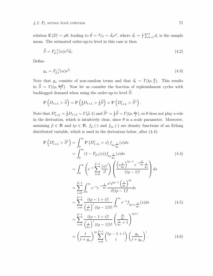
4.2. P1 service level criterion 71
relation E [D] = ρθ, leading to θ = dt/ρ = dtν2, where dt =
1t
∑ti=1 di is the sample
mean. The estimated order-up-to level in this case is then
S = F−1ρ,1 (α)ν
2dt. (4.2)
Define
gα = F−1ρ,1 (α)ν
2. (4.3)
Note that gα consists of non-random terms and that dt ∼ Γ(tρ, θt). This results
in S ∼ Γ(tρ, gαθt). Now let us consider the fraction of replenishment cycles with
backlogged demand when using the order-up-to level S:
P
(D1+L > S
)= P
(1θD1+L > 1
θS)= P
(D∗
1+L > S∗).
Note that D∗1+L = 1
θD1+L ∼ Γ(ρ, 1) and S∗ = 1
θS ∼ Γ(tρ, gα
t), so θ does not play a role
in the derivation, which is intuitively clear, since θ is a scale parameter. Moreover,
assuming ρ ∈ N and tρ ∈ N, fρ,·(·) and ftρ,·(·) are density functions of an Erlang
distributed variable, which is used in the derivation below, after (4.4):
P
(D∗
1+L > S∗)=
∫ ∞
0
P(D∗
1+L > s)ftρ,
tgα
(s)ds
=
∫ ∞
0
(1− Fρ,1(s))ftρ, tgα
(s)ds (4.4)
=
∫ ∞
0
(e−s
ρ−1∑
i=0
(s)i
i!
)
(s tgα
)tρ−1
e−s
tgα t
gα
(tρ− 1)!
ds
=
ρ−1∑
i=0
∫ ∞
0
e−se−s
tgα
sistρ−1(
tgα
)tρ
i!(tρ− 1)!ds
=
ρ−1∑
i=0
(tρ− 1 + i)!(
tgα
)i(tρ− 1)!i!
∫ ∞
0
e−sftρ+i,
tgα
(s)ds (4.5)
=
ρ−1∑
i=0
(tρ− 1 + i)!(
tgα
)i(tρ− 1)!i!
(tgα
tgα
+ 1
)tρ+i
=
(t
t+ gα
)tρ ρ−1∑
i=0
(tρ− 1 + i
i
)(gα
t+ gα
)i
. (4.6)

72 Chapter 4. Gamma demand with unknown demand parameters
Note that the integral part of (4.5) is the Laplace-Stieltjes transform of an Erlang-
(tρ + i) distribution. Now consider the special case of exponentially distributed
demand (ρ = 1) and zero lead time. Then gα = − ln(1− α) and (4.6) simplifies to
P
(D∗
1+L > S∗)=
(t
t+ gα
)t
=
(t
t− ln(1− α)
)t
.
Now we prove that the desired service level is not reached, in other words that
( tt−ln(1−α)
)t > 1 − α. The left hand side of this equation is a function of t and α:
h(t, α) = tt−ln(1−α)
)t. A graph of this function illustrates that indeed h(t, α) has 1−α
as its asymptote and reaches this asymptote from above; see Figure 4.1. Note that
α = 0.90α = 0.95α = 0.99
t
h(t,α
)
0 20 40 60 80 1000
0.05
0.1
0.15
0.2
0.25
0.3
Figure 4.1: The function h(t, α) for three different values of α and its asymptote.
the difference between the attained stock out probability (h(t, α)) and the desired
stock out probability (1 − α) is large when t is small, so it is not negligible. The
conjecture h(t, α) > 1 − α can be rewritten as ( t+ln((1−α)−1)t
)t < (1 − α)−1; note that
the left hand side is increasing in t. We finish our derivation as follows:
(1 +
ln(
11−α
)
t
)t
< limt→∞
(1 +
ln(
11−α
)
t
)t
= eln(
11−α
)
=1
1− α.
So in case of exponentially distributed demand and zero lead time, the desired service
level will not be attained and the underperformance is larger if t is smaller. If we
would replace α by α′ = 1−exp(t(1−(1−α)−1/t)), where obviously α′ > α, the desired
service would be attained again. Unfortunately, we cannot find such analytical results
if L > 0 or if ρ ∈ N/{1}.

4.2. P1 service level criterion 73
Now let us assume that ρ ∈ N and tρ ∈ N, with ρ ≥ 2. In this case we can
use (4.6) to investigate the attained service level numerically. These calculations,
not shown here, indicate that at low desired service levels the attained service level
exceeds the desired one, while this reverses at higher values of α. If α approximates
either 0 or 1, the attained service level approximates the desired one. This is easily
explained: if α = 0, gα = 0 and thus S = 0, so demand is not satisfied in any period.
On the other hand, if α = 1, gα → ∞ and thus S → ∞. In that case we can always
satisfy demand. Further, there is one α ∈ (0, 1) such that the attained service equals
the desired service level. These breakeven points are shown in Table 4.1 for several
combinations of ρ, t and L. Table 4.1 clearly shows that the breakeven point gets
L = 0 L = 1 L = 3ρ t = 2 t = 10 t = 20 t = 2 t = 10 t = 20 t = 2 t = 10 t = 202 0.2499 0.2612 0.2627 0.3288 0.3474 0.3500 0.3688 0.3932 0.39716 0.3729 0.3817 0.3828 0.4055 0.4172 0.4189 0.4253 0.4400 0.442310 0.4038 0.4107 0.4116 0.4274 0.4366 0.4380 0.4423 0.4537 0.455620 0.4329 0.4380 0.4387 0.4489 0.4556 0.4565 0.4593 0.4674 0.468750 0.4579 0.4612 0.4616 0.4678 0.4720 0.4727 0.4743 0.4794 0.4803
Table 4.1: Values of α for which the non-stock-out probability using order-up-to level Sequals α (ρ known).
higher if ρ is larger, if t is larger or if L is larger. It also appears to converge to
some value if ρ increases. In that case the coefficient of variation gets smaller and
the gamma distribution looks more and more like a normal distribution. For this
distribution it can easily be shown that the breakeven point is at α = 0.50 (see (3.2)
in Section 3.2).
In the remainder of this section and in Section 4.3 we will consider five different
attained service levels. The notation of these service levels is denoted in Table 4.2.
α0(β0): Attained service when θ unknown, but ρ known;
α1(β1): Attained service when ρ and θ unknown and using α(β);
α2(β2): Attained service when ρ and θ unknown and using α′(β ′);
α3(β3): Attained service when using correction function kα(ρ, t, α, L)(kβ(ρ, t, β, L));
α4(β4): Attained service when using correction function kα(ρ, t, α, L)(kβ(ρ, t, β, L)).
Table 4.2: The attained service levels discussed in Sections 4.2 and 4.3 and their notation.

74 Chapter 4. Gamma demand with unknown demand parameters
ρL
α0
t = 4t = 8t = 12
α=0.90
13
4413
16517
01
46
0.7
0.8
0.9
ρL
δ α(α
0)
t = 4t = 8t = 12
α=0.90
1344
13
16517
01
46
0
1
2
3
ρL
α0
t = 4t = 8t = 12
α=0.95
13
4413
16517
01
46
0.7
0.8
0.9
ρL
δ α(α
0)
t = 4t = 8t = 12
α=0.95
1344
13
16517
01
46
0
2
4
6
ρL
α0
t = 4t = 8t = 12
α=0.99
13
4413
16517
01
46
0.8
0.9
1
ρL
δ α(α
0)
t = 4t = 8t = 12
α=0.99
1344
13
16517
01
46
0
10
20
Figure 4.2: Attained service (α0) and relative deviation (δα(α0)) for non-integer butknown values of ρ.
Now let us consider ρ > 0 and tρ > 0, not necessarily integer. In this case it is no
longer possible to derive a closed-form expression, but we can numerically evaluate
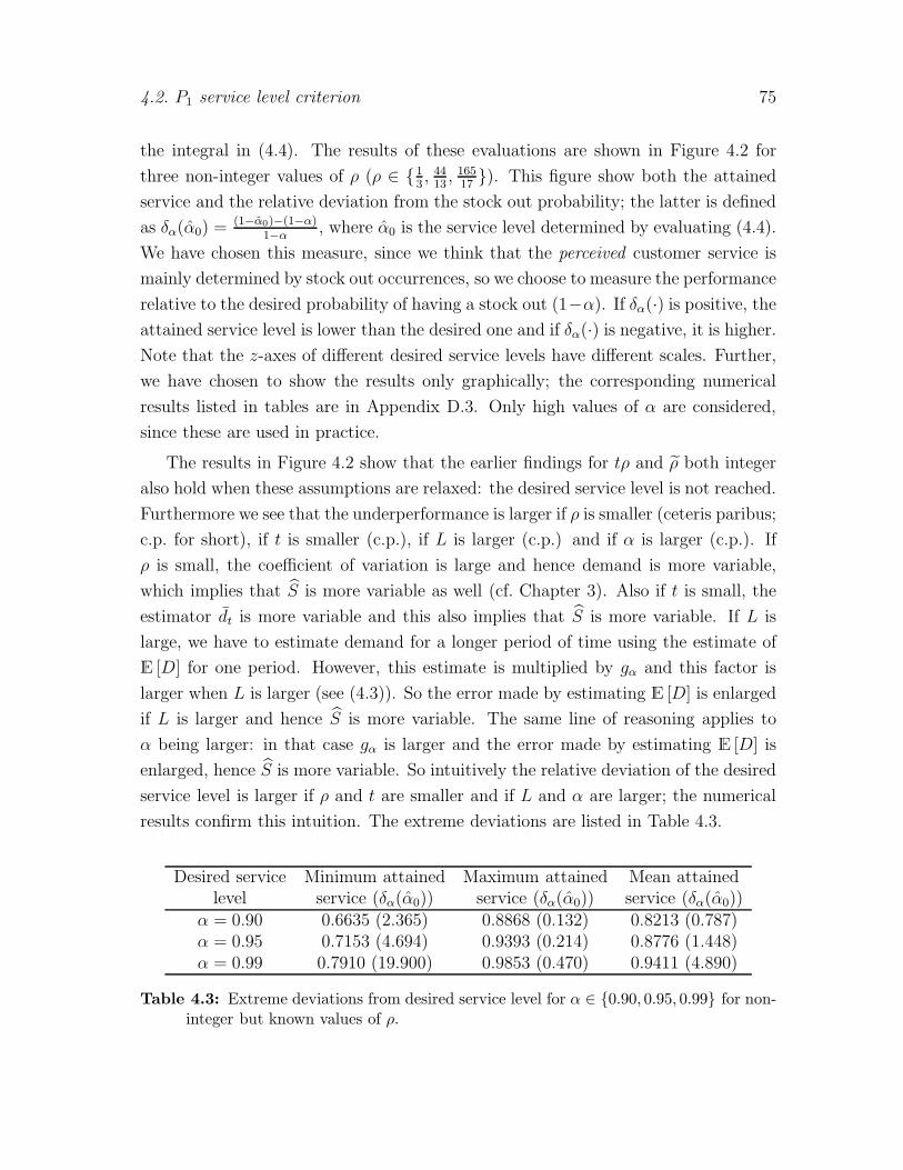
4.2. P1 service level criterion 75
the integral in (4.4). The results of these evaluations are shown in Figure 4.2 for
three non-integer values of ρ (ρ ∈ {13, 4413, 165
17}). This figure show both the attained
service and the relative deviation from the stock out probability; the latter is defined
as δα(α0) =(1−α0)−(1−α)
1−α, where α0 is the service level determined by evaluating (4.4).
We have chosen this measure, since we think that the perceived customer service is
mainly determined by stock out occurrences, so we choose to measure the performance
relative to the desired probability of having a stock out (1−α). If δα(·) is positive, theattained service level is lower than the desired one and if δα(·) is negative, it is higher.Note that the z-axes of different desired service levels have different scales. Further,
we have chosen to show the results only graphically; the corresponding numerical
results listed in tables are in Appendix D.3. Only high values of α are considered,
since these are used in practice.
The results in Figure 4.2 show that the earlier findings for tρ and ρ both integer
also hold when these assumptions are relaxed: the desired service level is not reached.
Furthermore we see that the underperformance is larger if ρ is smaller (ceteris paribus;
c.p. for short), if t is smaller (c.p.), if L is larger (c.p.) and if α is larger (c.p.). If
ρ is small, the coefficient of variation is large and hence demand is more variable,
which implies that S is more variable as well (cf. Chapter 3). Also if t is small, the
estimator dt is more variable and this also implies that S is more variable. If L is
large, we have to estimate demand for a longer period of time using the estimate of
E [D] for one period. However, this estimate is multiplied by gα and this factor is
larger when L is larger (see (4.3)). So the error made by estimating E [D] is enlarged
if L is larger and hence S is more variable. The same line of reasoning applies to
α being larger: in that case gα is larger and the error made by estimating E [D] is
enlarged, hence S is more variable. So intuitively the relative deviation of the desired
service level is larger if ρ and t are smaller and if L and α are larger; the numerical
results confirm this intuition. The extreme deviations are listed in Table 4.3.
Desired service Minimum attained Maximum attained Mean attainedlevel service (δα(α0)) service (δα(α0)) service (δα(α0))
α = 0.90 0.6635 (2.365) 0.8868 (0.132) 0.8213 (0.787)α = 0.95 0.7153 (4.694) 0.9393 (0.214) 0.8776 (1.448)α = 0.99 0.7910 (19.900) 0.9853 (0.470) 0.9411 (4.890)
Table 4.3: Extreme deviations from desired service level for α ∈ {0.90, 0.95, 0.99} for non-integer but known values of ρ.
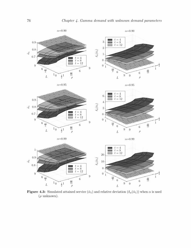
76 Chapter 4. Gamma demand with unknown demand parameters
ρL
α1
α=0.90
t = 4t = 8t = 12
121
4413
69
01
133
69
0.7
0.8
0.9
ρL
δ α(α
1)
12
α=0.90
t = 4t = 8t = 12
144136
9
0 1133 6
9
0
1
2
3
ρL
α1
α=0.95
t = 4t = 8t = 12
121
4413
69
01
133
69
0.7
0.8
0.9
ρL
δ α(α
1)
12
α=0.95
t = 4t = 8t = 12
144136
9
0 1133 6
9
0
2
4
6
ρL
α1
α=0.99
t = 4t = 8t = 12
121
4413
69
01
133
69
0.8
0.9
1
ρL
δ α(α
1)
12
α=0.99
t = 4t = 8t = 12
144136
9
0 1133 6
9
0
10
20
Figure 4.3: Simulated attained service (α1) and relative deviation (δα(α1)) when α is used(ρ unknown).

4.2. P1 service level criterion 77
Both θ and ρ unknown
In the first part of this section ρ is assumed to be known. In the remainder of this
subsection this assumption is relaxed, hence, an estimate of ρ is needed. The sample
mean and sample variance(s2t =
1t−1
∑ti=1(di − dt)
2)are used to estimate ρ and θ:
ρ = d2t/s2t and θ = s2t/dt. Using these in the estimate of the order-up-to level results
in S = θF−1(1+L)ρ,1(α) and this is no longer gamma distributed. So derivations become
intractable and hence simulation is used to determine the attained service level α1
(see Appendix D.1). This simulation is restricted to high values of α, since values
lower than 0.90 will not often be used in practice. The simulation has n = 100, 000
replicates for each combination of ρ, t, α and L and its results are displayed in Figure
4.3. Remember that θ is a scale parameter and hence has no influence on the attained
service level. Note that the scales of the z-axes of the graphs equal the scales of the
z-axes of the graphs of Figure 4.2 with corresponding α-values for easy comparison.
The same holds for the z-axes of Figures 4.4 and 4.6. Figure 4.3 clearly show that in
all cases considered the desired service level is not reached. The underperformance
again is larger if ρ is smaller (c.p.), if t is smaller (c.p.), if L is larger (c.p.) and if α
is larger (c.p.). The extreme deviations and mean attained service level are displayed
in Table 4.4.
Desired service Minimum attained Maximum attained Mean attainedlevel service (δα(α1)) service (δα(α1)) service (δα(α1))
α = 0.90 0.6144 (2.856) 0.8847 (0.153) 0.8089 (0.911)α = 0.95 0.6575 (5.850) 0.9366 (0.268) 0.8624 (1.752)α = 0.99 0.7244 (26.560) 0.9819 (0.810) 0.9253 (6.470)
Table 4.4: Extreme deviations from desired service level for α ∈ {0.90, 0.95, 0.99} when α
is used (ρ unknown).
A first improvement
In the case of an exponential distribution (ρ = 1) and zero lead time, using α′ instead
of α ascertains that the desired service level is met. Using α′ while ρ is unknown
and L ≥ 0 will probably not lead to meeting the desired service level, but since
α′ > α it certainly increases the attained service level, denoted by α2. The results
of replacing α by α′ are shown in Figure 4.4; Table 4.5 displays the extreme devi-

78 Chapter 4. Gamma demand with unknown demand parameters
ρL
α2
α=0.90
t = 4t = 8t = 12
121
4413
69
01
133
69
0.7
0.8
0.9
ρL
δ α(α
2)
12
α=0.90
t = 4t = 8t = 12
144136
9
0 1133 6
9
0
1
2
3
ρL
α2
α=0.95
t = 4t = 8t = 12
121
4413
69
01
133
69
0.7
0.8
0.9
ρL
δ α(α
2)
12
α=0.95
t = 4t = 8t = 12
144136
9
0 1133 6
9
0
2
4
6
ρL
α2
α=0.99
t = 4t = 8t = 12
121
4413
69
01
133
69
0.8
0.9
1
ρL
δ α(α
2)
12
α=0.99
t = 4t = 8t = 12
144136
9
0 1133 6
9
0
10
20
Figure 4.4: Simulated attained service (α2) and relative deviation (δα(α2)) when α′ isused (ρ unknown).
ations. Figure 4.4 indeed shows that the performance improves significantly compared
to using α; improvements range from almost 18% up to almost 80%. These relative
improvements, denoted by Iα(αi, αj), are measured by considering the percentage

4.2. P1 service level criterion 79
Desired service Minimum attained Maximum attained Mean attainedlevel service (δα(α2)) service (δα(α2)) service (δα(α2))
α = 0.90 0.6624 (2.376) 0.8975 (0.025) 0.8382 (0.618)α = 0.95 0.7197 (4.606) 0.9478 (0.044) 0.8933 (1.134)α = 0.99 0.8134 (17.660) 0.9881 (0.190) 0.9546 (3.540)
Table 4.5: Extreme deviations from desired service level for α ∈ {0.90, 0.95, 0.99} whenα′ is used (ρ unknown).
change in the attained stock out probability. Let αi denote the attained service level
using the order-up-to level determined by method i, here α1, while αj denotes the
attained service level using method j, α2. The improvements Iα(αi, αj) are calculated
using
Iα(αi, αj) =δα(αi)− δα(αj)
δα(αi)· 100% =
αj − αi
α− αi· 100%.
So if Iα(αi, αj) is between 0 and 100%, αj is closer to the desired service level than
αi. If it is negative, this reverses, i.e., the αi is closer to the desired service level
than αj. If Iα(αi, αj) is larger than 100%, using method j instead of i results in
overperformance, if under i there was underperformance and vice versa. If it is
smaller than 200%, αj is closer to the desired service level compared to αi and this
reverses if the improvement is larger than 200%.
Four cases are considered in detail; see Table 4.6. In the first case the attained
α ρ t L α1 (δα(α1)) α2 (δα(α2)) Iα(α1, α2)
0.90 4413
8 413
0.8016 ( 0.984) 0.8350 ( 0.650) 33.94%0.95 9 12 1 0.9178 ( 0.644) 0.9375 ( 0.250) 61.18%0.95 6 12 0 0.9262 ( 0.464) 0.9449 ( 0.102) 78.57%0.99 1
24 6 0.7579 (23.210) 0.8445 (14.550) 37.31%
Table 4.6: Examples of improvement of attained service using α′ instead of α.
service level increases from 0.8016 (δα(α1) = 0.984) to 0.8350 (δα(α2) = 0.650), which
is an improvement of (0.8350− 0.8016)/(0.90− 0.8016) · 100% = 33.94%. Using the
relative deviations (δα(·)), the same improvement is found: (0.984 − 0.650)/0.984 ·100% = 33.94%. In the second case one can see that, although the attained service
level is already pretty close to the desired service level (compared to the first and
fourth case), a large improvement is possible using α′ instead of α. This leads to
almost reaching the desired service level. In the third case the desired service level

80 Chapter 4. Gamma demand with unknown demand parameters
is reached even closer. In the fourth case the attained service level is a lot closer to
the desired service level, but there is still a large underperformance. This case has
the most difficult parameter setting: both ρ and t are small while both α and L are
large.
4.2.2 Determining the correction
As seen in Subsection 4.2.1 the desired service level is not met when using estimates in
the determination of the order-up-to level. The attained service level can be improved
by using α′ instead of α, but still the desired service level is not reached. Another
idea could be to use (an estimate of) the variance of the forecast error instead of
the variance of demand (cf. Chapter 3). We have tried using this correction, but
unfortunately simulation indicates no consistent improvement and hence we decided
to consider other methods to improve the attained service level.
In this section it is shown that the attained service level is further improved
(compared to only using α′ instead of α) by using a multiplicative correction. That
is, the estimated order-up-to level is multiplied by a certain factor that depends on
the value of ρ, t, α and L (used parameter values are listed in Table 4.7). We also
Parameter Values used in simulationρ 0.5, 1, 2, 4, 6, 8, 10t 4, 6, 8, 10, 12, 20α 0.90, 0.91, 0.92, 0.93, 0.94, 0.95, 0.96, 0.97, 0.98, 0.99L 0, 0.5, 1, 3, 6
Table 4.7: Parameter values used for finding correction values.
tried to use a additive correction, as is used in Chapter 3, but this did not lead to
consistent improvements. This might be intuitively explained by the functional form
of the order-up-to level: if we assume gamma distributed demand, the order-up-to
level is a multiplication of several terms, see (4.2). On the other hand, if demand
is assumed to be normally distributed, the order-up-to level is a sum of two terms,
see (3.1) and (3.4). Hence, a multiplicative correction might perform better for the
gamma distribution, while an additive correction might be more suitable for the
normal distribution.
Simulation is used to find the multiplication factor. The values of the corrections
are found by first determining the order-up-to levels one would get while using ρ, θ
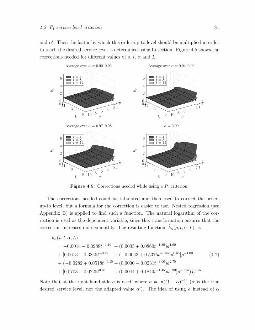
4.2. P1 service level criterion 81
and α′. Then the factor by which this order-up-to level should be multiplied in order
to reach the desired service level is determined using bi-section. Figure 4.5 shows the
corrections needed for different values of ρ, t, α and L.
Average over α = 0.90–0.93
ρL
kα
12
t = 4t = 8t = 12
1246810
0 121
3
6
0
2
4
6
Average over α = 0.94–0.96
ρL
kα
12
t = 4t = 8t = 12
1246810
0 121
3
6
0
2
4
6
replacemen
Average over α = 0.97–0.98
ρL
kα
12
t = 4t = 8t = 12
1246810
0 121
3
6
0
2
4
6
α = 0.99
ρL
kα
12
t = 4t = 8t = 12
1246810
0 121
3
6
0
2
4
6
Figure 4.5: Corrections needed while using a P1 criterion.
The corrections needed could be tabulated and then used to correct the order-
up-to level, but a formula for the correction is easier to use. Nested regression (see
Appendix B) is applied to find such a function. The natural logarithm of the cor-
rection is used as the dependent variable, since this transformation ensures that the
correction increases more smoothly. The resulting function, kα(ρ, t, α, L), is
kα(ρ, t, α, L)
= −0.0014− 0.0988t−1.10 + (0.0005 + 0.0860t−1.80)a1.90
+ [0.0613− 0.3845t−0.45 + (−0.0043 + 0.5375t−0.85)a0.85]ρ−1.00 (4.7)
+(−0.0282 + 0.0518t−0.15 + (0.0000− 0.0231t−3.00)a2.75
+ [0.0703− 0.0225t0.35 + (0.0044 + 0.1840t−1.45)a0.90]ρ−0.75)L0.55.
Note that at the right hand side a is used, where a = ln((1 − α)−1) (α is the true
desired service level, not the adapted value α′). The idea of using a instead of α

82 Chapter 4. Gamma demand with unknown demand parameters
originates from the fact that gα = a in case of exponentially distributed demand and
zero lead time, hence a influences the order-up-to level directly. In short, (4.7) has
been found as follows: we first choose only one dependent variable (L in case of (4.7))
and regress that on the logarithm of the correction needed, with different values for
the power. We choose the power that results in the lowest sum of squared errors.
Next we choose a second variable (ρ) and that is regressed on the coefficients found
in the first regression. Also the third (a) and fourth (t) variable are treated in this
manner; see Appendix B for a detailed description of the method. We choose to use
this method, instead of, e.g., stepwise linear regression, because of the way the values
of the powers are determined. Note that there are 4! = 24 orderings for choosing the
parameters; we have tried all orderings and have selected the best.
Using (4.7) on the parameter values listed in Table 4.7 results in an R2 (coefficient
of determination) of 0.9988 (adjusted R2 = 0.9987), which is very high. However,
using (4.7) implies that ρ is known, which is obviously not true in practice. We solve
this by using the estimate for ρ, but that will be at the expense of a lower attained
service. The size of the difference between the attained and desired service level is
determined with help of simulation (n = 100, 000) using (4.7). The order-up-to level
in this simulation is thus determined by S · exp(kα(ρ, t, α, L)). Figure 4.6 displays
the resulting attained service levels (α3) and the corresponding relative deviations
(δα(α3)); the extreme deviations are listed in Table 4.8. This simulation shows that
Desired service Minimum attained Maximum attained Mean attainedlevel service (δα(α3)) service (δα(α3)) service (δα(α3))
α = 0.90 0.8387 (0.613) 0.9034 (-0.034) 0.8909 (0.091)α = 0.95 0.8899 (1.202) 0.9509 (-0.018) 0.9391 (0.218)α = 0.99 0.9479 (4.210) 0.9901 (-0.010) 0.9826 (0.740)
Table 4.8: Extreme deviations from desired service level for α ∈ {0.90, 0.95, 0.99} using
S · ekα(ρ,t,α,L).
indeed the desired service level is reached more closely; in case of ρ large, α = 0.90
and t = 12 the desired service is even reached completely. Additional improvements
for the remainder of the cases range from 60% to 99%. Total improvements for
the cases in which the desired service level is not met range from 76% up to 99%.

4.2. P1 service level criterion 83
ρL
α3
α=0.90
t = 4t = 8t = 12
121
4413
69
01
133
69
0.7
0.8
0.9
ρL
δ α(α
3)
12
α=0.90
t = 4t = 8t = 12
144136
9
0 1133 6
9
0
1
2
3
ρL
α3
α=0.95
t = 4t = 8t = 12
121
4413
69
01
133
69
0.7
0.8
0.9
ρL
δ α(α
3)
12
α=0.95
t = 4t = 8t = 12
144136
9
0 1133 6
9
0
2
4
6
ρL
α3
α=0.99
t = 4t = 8t = 12
121
4413
69
01
133
69
0.8
0.9
1
ρL
δ α(α
3)
12
α=0.99
t = 4t = 8t = 12
144136
9
0 1133 6
9
0
10
20
Figure 4.6: Simulated attained service (α3) and relative deviation (δα(α3)) using S ·ekα(ρ,t,α,L).
See Table 4.9 for the four cases that were also considered in Table 4.6. In the first
case the attained service level is improved a lot and the desired service level is almost

84 Chapter 4. Gamma demand with unknown demand parameters
α ρ t L α2 (δα(α2)) α3 (δα(α3)) Iα(α2, α3) Iα(α1, α3)
0.90 4413
8 413
0.8350 ( 0.650) 0.8911 (0.089) 86.31% 90.96%0.95 9 12 1 0.9375 ( 0.250) 0.9498 (0.004) 98.40% 99.38%0.95 6 12 0 0.9449 ( 0.102) 0.9493 (0.014) 86.27% 97.06%0.99 1
24 6 0.8445 (14.550) 0.9508 (3.920) 73.06% 83.11%
Table 4.9: Examples of improvement of attained service using the correction kα(ρ, t, α, L)instead of only α′.
reached. In the second and third case we can state that it actually is reached and in
the fourth case we again see a large improvement upon the situation without using a
correction, but unfortunately the underperformance is still quite large in this case.
The fact that the desired service level is not reached completely in almost all
cases (see Figure 4.6), is due to using ρ instead of ρ. If this true value could be used,
simulation shows (resulting in attained service levels α4) that the desired service level
is reached; the extreme deviations are denoted in Table 4.10.
Desired service Minimum attained Maximum attained Mean attainedlevel service (δα(α4)) service (δα(α4)) service (δα(α4))
α = 0.90 0.8972 (0.028) 0.9109 (-0.109) 0.9013 (-0.013)α = 0.95 0.9462 (0.076) 0.9556 (-0.112) 0.9499 (0.002)α = 0.99 0.9886 (0.140) 0.9919 (-0.190) 0.9898 (0.020)
Table 4.10: Extreme deviations from desired service level for α ∈ {0.90, 0.95, 0.99} using
S · ekα(ρ,t,α,L).
We determined the estimates of the attained service in all our simulations in
Section 4.2 using independent samples (each estimate was determined using different
simulated demand periods). However, in practice one uses a rolling horizon. Our
simulations have been repeated with a rolling horizon and the results are similar.
4.3 P2 service level criterion
This section considers the P2 service level criterion, so we need to find an order-up-
to level S such that E [(D1+L − S)+] − E [(DL − S)+] = (1 − β)E [D]. Note that
shortages at the start of a replenishment cycle are included and if L = 0, the second
expectation vanishes. When assuming that both parameters are known, it is not
difficult to find the order-up-to level that satisfies this criterion. We have to find the

4.3. P2 service level criterion 85
value of S that satisfies the equality above. First note that the left hand side can be
rewritten to
E[(D1+L − S)+
]− E
[(DL − S)+
]
=
∫ ∞
S
(x− S)fρ,θ(x)dx−∫ ∞
S
(x− S)fLρ,θ(x)dx =: Lρ,θ(S)− LLρ,θ(S).
It is well known that Lρ,θ(y) =∫∞y(x−y)fρ,θ(x)dx = ρθ[1−Fρ+1,θ(y)]−y[1−Fρ,θ(y)].
Note that there is no closed-form expression for the order-up-to level in general, hence
we need to solve it numerically. However, if an exponential distribution is assumed,
the order-up-to level using the P2 criterion equals the order-up-to level using the P1
criterion when α = β (see Appendix D.2). Hence, if ρ = 1, S = θF−11+L,1(β).
4.3.1 Using estimates in determining the order-up-to level
The method described above can only be used when ρ and θ are known. This sub-
section discusses the effect of estimating ρ and θ on the attained P2 service.
Only θ unknown
Let us first consider the case that only θ is unknown and ρ = 1, hence we have
exponentially distributed demand during the review period. Since in the case of
exponentially distributed demand the theoretically correct order-up-to levels of the
P1 and the P2 criterion are equal, the order-up-to level in case of the P2 criterion can
be estimated by S = gβdt , where gβ = F−11+L,1(β). Then it is known that S ∼ Γ(t,
gβθ
t).
The attained service, using again the fact that θ is a scale parameter and S∗ = 1θS,
is (using relation (D.2) in Appendix D.2)
E
[(D∗
1+L − S∗)+]− E
[(D∗
L − S∗)+]
= E
[E
[(D∗
1+L − S∗)+|S∗]− E
[(D∗
L − S∗)+|S∗]]
(D.2)= E
[P
(D∗
1+L > S∗|S∗)]
= P
(D∗
1+L > S∗)
=
(t
t+ gβ
)t L∑
i=0
(t− 1 + i
i
)(gβ
t+ gβ
)iL=0=
(t
t + gβ
)t
> 1− β.
Hence, in case of zero lead time the attained service always falls short of the desired
one. In fact, as long as we are considering exponentially distributed demand during

86 Chapter 4. Gamma demand with unknown demand parameters
ρL
β0
β=0.90
t = 4t = 8t = 12
121
4413
69
01
133
69
0.6
0.7
0.8
0.9
ρL
δ β(β
0)
12
β=0.90
t = 4t = 8t = 12
144136
9
0 1133 6
9
0
1
2
3
ρL
β0
β=0.95
t = 4t = 8t = 12
121
4413
69
01
133
69
0.7
0.8
0.9
ρL
δ β(β
0)
12
β=0.95
t = 4t = 8t = 12
144136
9
0 1133 6
9
0
2
4
6
ρL
β0
β=0.99
t = 4t = 8t = 12
121
4413
69
01
133
69
0.8
0.9
1
ρL
δ β(β
0)
12
β=0.99
t = 4t = 8t = 12
144136
9
0 1133 6
9
0
10
20
Figure 4.7: Simulated attained service (β0) and relative deviation (δβ(β0)) for non-integerbut known values of ρ.
the review period, the results of the P1 criterion also hold for the P2 criterion. Un-
fortunately, if ρ 6= 1, no tractable results can be derived, due to the non-existence
of a closed-form expression for S. Hence, simulation is used in this case (again with

4.3. P2 service level criterion 87
n = 100, 000 replicates) to obtain the performance of using an estimate for θ (θ = dtρ)
in determining the order-up-to level. Note that ρ is still assumed to be known.
The relative deviation from the desired fraction of backlogged demand, denoted by
δβ(β0) = (1−β0)−(1−β)1−β
, where β0 is the service attained in simulation (see Appendix
D.1), is shown in Figure 4.7; Table 4.11 displays the extreme deviations from the
desired service level and the mean attained service levels. Note that the scales of
Desired service Minimum attained Maximum attained Mean attained
level service (δβ(β0)) service (δβ(β0)) service (δβ(β0))β = 0.90 0.6491 (2.509) 0.8964 (0.036) 0.8303 (0.697)β = 0.95 0.6987 (5.026) 0.9472 (0.056) 0.8863 (1.274)β = 0.99 0.7794 (21.060) 0.9883 (0.170) 0.9487 (4.130)
Table 4.11: Extreme deviations from desired service level for β ∈ {0.90, 0.95, 0.99} fornon-integer but known values of ρ.
the graphs in Figure 4.7 of the z-axes vary across the different desired service levels.
This simulation shows that the desired service level is not met when we have to use
an estimate for θ instead of the true value. Also the underperformance is larger if ρ
is smaller (c.p.), if t is smaller (c.p.), if L is larger (c.p.) and if β is larger (c.p.).
Both θ and ρ unknown
If also ρ is assumed to be unknown, that parameter has to be estimated as well. The
estimates for the parameters ρ and θ are ρ =d2ts2t
and θ =s2tdt, where dt is the sample
mean and s2t the sample variance. The order-up-to level based on these estimates (S)
is determined by solving (using binary search)
L(1+L)ρ,1(S∗)− LLρ,1(S
∗) = (1− β)ρ (4.8)
to get S∗ and then S = θS∗. Note that the left hand side of (4.8) is decreasing in
S∗, since it denotes the amount of backlogged demand, hence using binary search
is appropriate. Next, simulation is used to estimate the performance of the order-
up-to level determined in this way; β1 denotes the attained service. The results of
this simulation, again based on n = 100, 000 replicates, are shown in Figure 4.8.
The z-axes in Figure 4.8 equal the z-axes in Figure 4.7 for easy comparison, just
as the z-axes in Figures 4.9 and 4.11. Comparing Figure 4.8 to Figure 4.7 clearly
shows that the underperformance is larger if both ρ and θ are assumed to be unknown.

88 Chapter 4. Gamma demand with unknown demand parameters
ρL
β1
β=0.90
t = 4t = 8t = 12
121
4413
69
01
133
69
0.6
0.7
0.8
0.9
ρL
δ β(β
1)
12
β=0.90
t = 4t = 8t = 12
144136
9
0 1133 6
9
0
1
2
3
ρL
β1
β=0.95
t = 4t = 8t = 12
121
4413
69
01
133
69
0.7
0.8
0.9
ρL
δ β(β
1)
12
β=0.95
t = 4t = 8t = 12
144136
9
0 1133 6
9
0
2
4
6
ρL
β1
β=0.99
t = 4t = 8t = 12
121
4413
69
01
133
69
0.8
0.9
1
ρL
δ β(β
1)
12
β=0.99
t = 4t = 8t = 12
144136
9
0 1133 6
9
0
10
20
Figure 4.8: Simulated attained service (β1) and relative deviation (δβ(β1)) when β is used(ρ unknown).
Furthermore, we again see that the underperformance is larger when ρ is smaller
(c.p.), when t is smaller (c.p.), when L is larger (c.p.) and when β is larger (c.p.).
The extreme deviations from the desired service level are displayed in Table 4.12.

4.3. P2 service level criterion 89
Desired service Minimum attained Maximum attained Mean attained
level service (δβ(β1)) service (δβ(β1)) service (δβ(β1))β = 0.90 0.5970 (3.030) 0.8938 (0.062) 0.8074 (0.926)β = 0.95 0.6381 (6.238) 0.9434 (0.132) 0.8614 (1.772)β = 0.99 0.7115 (27.850) 0.9853 (0.470) 0.9251 (6.490)
Table 4.12: Extreme deviations from desired service level for β ∈ {0.90, 0.95, 0.99} whenβ is used (ρ unknown).
A first improvement
In case of exponential demand and zero lead time under the P1 criterion the desired
service level could be attained by using α′ instead of α. Since the order-up-to levels
under the P1 and P2 criterion are equal in case of exponential demand, the same holds
here; i.e., if β is replaced by β ′ = 1− exp(t(1− (1− β)−1/t)), the desired service level
is met again, when lead time is zero. Of course, when demand is not exponentially
distributed, this does not hold, but we can use this correction as a first improvement.
The attained service level (β2) and relative deviation (δβ(β2)) when using β ′ in-
stead of β are shown in Figure 4.9; the extreme deviations in Table 4.13. Figure
4.9 clearly shows that, although the desired service is still not met (except for some
Desired service Minimum attained Maximum attained Mean attained
level service (δβ(β2)) service (δβ(β2)) service (δβ(β2))β = 0.90 0.6472 (2.528) 0.9234 (-0.234) 0.8371 (0.629)β = 0.95 0.7019 (4.962) 0.9616 (-0.232) 0.8927 (1.146)β = 0.99 0.8026 (18.740) 0.9910 (-0.100) 0.9543 (3.570)
Table 4.13: Extreme deviations from desired service level for β ∈ {0.90, 0.95, 0.99} whenβ′ is used (ρ unknown).
cases where ρ large, L = 0 and t large), the attained service is significantly im-
proved. In the cases where the desired service level is not met, improvements range
from 16% to 99%; see Table 4.14 for the four cases of the previous examples. The
improvements shown in this table are actually quite similar compared to the improve-
ments for the P1 criterion, except for the third case. In this case the desired service
level is not only met, but even exceeded, which leads to an improvement of more
than 100%, i.e., overperformance. Still, the attained service level is closer than be-
fore, since the absolute deviation now is 0.0038, while without using β ′ it was 0.0134.

90 Chapter 4. Gamma demand with unknown demand parameters
ρL
β2
β=0.90
t = 4t = 8t = 12
121
4413
69
01
133
69
0.6
0.7
0.8
0.9
ρL
δ β(β
2)
12
β=0.90
t = 4t = 8t = 12
144136
9
0 1133 6
9
0
1
2
3
ρL
β2
β=0.95
t = 4t = 8t = 12
121
4413
69
01
133
69
0.7
0.8
0.9
ρL
δ β(β
2)
12
β=0.95
t = 4t = 8t = 12
144136
9
0 1133 6
9
0
2
4
6
ρL
β2
β=0.99
t = 4t = 8t = 12
121
4413
69
01
133
69
0.8
0.9
1
ρL
δ β(β
2)
12
β=0.99
t = 4t = 8t = 12
144136
9
0 1133 6
9
0
10
20
Figure 4.9: Simulated attained service (β2) and relative deviation (δβ(β2)) when β′ isused (ρ unknown).
Therefore, the improvement is between 100% and 200%: the underperformance is
changed to overperformance, but the absolute deviation from the desired service
level is smaller. In the second case the desired service level is almost reached (closer
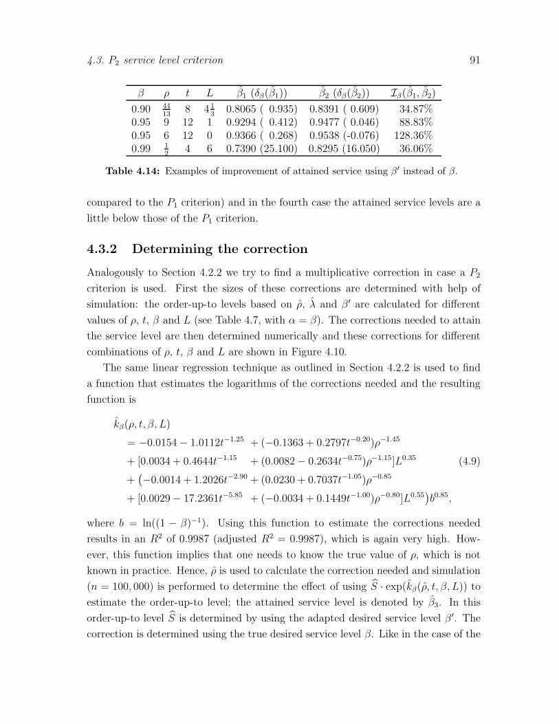
4.3. P2 service level criterion 91
β ρ t L β1 (δβ(β1)) β2 (δβ(β2)) Iβ(β1, β2)
0.90 4413
8 413
0.8065 ( 0.935) 0.8391 ( 0.609) 34.87%0.95 9 12 1 0.9294 ( 0.412) 0.9477 ( 0.046) 88.83%0.95 6 12 0 0.9366 ( 0.268) 0.9538 (-0.076) 128.36%0.99 1
24 6 0.7390 (25.100) 0.8295 (16.050) 36.06%
Table 4.14: Examples of improvement of attained service using β′ instead of β.
compared to the P1 criterion) and in the fourth case the attained service levels are a
little below those of the P1 criterion.
4.3.2 Determining the correction
Analogously to Section 4.2.2 we try to find a multiplicative correction in case a P2
criterion is used. First the sizes of these corrections are determined with help of
simulation: the order-up-to levels based on ρ, λ and β ′ are calculated for different
values of ρ, t, β and L (see Table 4.7, with α = β). The corrections needed to attain
the service level are then determined numerically and these corrections for different
combinations of ρ, t, β and L are shown in Figure 4.10.
The same linear regression technique as outlined in Section 4.2.2 is used to find
a function that estimates the logarithms of the corrections needed and the resulting
function is
kβ(ρ, t, β, L)
= −0.0154− 1.0112t−1.25 + (−0.1363 + 0.2797t−0.20)ρ−1.45
+ [0.0034 + 0.4644t−1.15 + (0.0082− 0.2634t−0.75)ρ−1.15]L0.35 (4.9)
+(−0.0014 + 1.2026t−2.90 + (0.0230 + 0.7037t−1.05)ρ−0.85
+ [0.0029− 17.2361t−5.85 + (−0.0034 + 0.1449t−1.00)ρ−0.80]L0.55)b0.85,
where b = ln((1 − β)−1). Using this function to estimate the corrections needed
results in an R2 of 0.9987 (adjusted R2 = 0.9987), which is again very high. How-
ever, this function implies that one needs to know the true value of ρ, which is not
known in practice. Hence, ρ is used to calculate the correction needed and simulation
(n = 100, 000) is performed to determine the effect of using S · exp(kβ(ρ, t, β, L)) toestimate the order-up-to level; the attained service level is denoted by β3. In this
order-up-to level S is determined by using the adapted desired service level β ′. The
correction is determined using the true desired service level β. Like in the case of the

92 Chapter 4. Gamma demand with unknown demand parameters
Average over β = 0.90–0.93
ρL
kβ
12
t = 4t = 8t = 12
1246810
0 121
3
6
0
2
4
6
Average over β = 0.94–0.96
ρL
kβ
12
t = 4t = 8t = 12
1246810
0 121
3
6
0
2
4
6
Average over β = 0.97–0.98
ρL
kβ
12
t = 4t = 8t = 12
1246810
0 121
3
6
0
2
4
6
β = 0.99
ρL
kβ
12
t = 4t = 8t = 12
1246810
0 121
3
6
0
2
4
6
Figure 4.10: Corrections needed while using a P2 criterion.
P1 criterion, the coefficients are rounded to 10−4. The results are shown in Figure 4.11;
the extreme deviations are in Table 4.15. This simulation shows that the desired ser-
vice level is reached more closely, but not reached completely yet; also in the few cases
it was reached when not using this correction function (β2; see Figure 4.9) the service
is not reached, since the correction needed is smaller than 1 for those cases. In general,
additional improvements range from only a few percent or even a little decline, in the
cases were the desired service level was (almost) met, to 94%. The total improvements
range from 66% to 94%. Table 4.16 shows the four cases we have considered earlier.
Desired service Minimum attained Maximum attained Mean attained
level service (δβ(β3)) service (δβ(β3)) service (δβ(β3))β = 0.90 0.8231 (0.769) 0.9066 (-0.066) 0.8859 (0.141)β = 0.95 0.8781 (1.438) 0.9541 (-0.082) 0.9360 (0.280)β = 0.99 0.9447 (4.530) 0.9908 (-0.080) 0.9810 (0.900)
Table 4.15: Extreme deviations from desired service level for β ∈ {0.90, 0.95, 0.99} using
S · ekβ(ρ,t,β,L).

4.3. P2 service level criterion 93
ρL
β3
β=0.90
t = 4t = 8t = 12
121
4413
69
01
133
69
0.6
0.7
0.8
0.9
ρL
δ β(β
3)
12
β=0.90
t = 4t = 8t = 12
144136
9
0 1133 6
9
0
1
2
3
ρL
β3
β=0.95
t = 4t = 8t = 12
121
4413
69
01
133
69
0.7
0.8
0.9
ρL
δ β(β
3)
12
β=0.95
t = 4t = 8t = 12
144136
9
0 1133 6
9
0
2
4
6
ρL
β3
β=0.99
t = 4t = 8t = 12
121
4413
69
01
133
69
0.8
0.9
1
ρL
δ β(β
3)
12
β=0.99
t = 4t = 8t = 12
144136
9
0 1133 6
9
0
10
20
Figure 4.11: Simulated attained service (β3) and relative deviation (δβ(β3)) using S ·ekβ(ρ,t,β,L).
In the first case the attained service level is improved upon considerably and the
desired service level is almost reached. In the second case we only see a minor
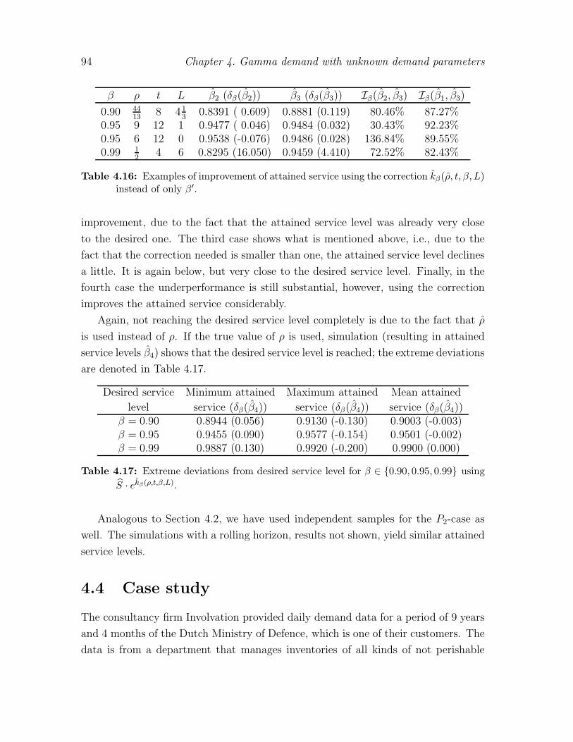
94 Chapter 4. Gamma demand with unknown demand parameters
β ρ t L β2 (δβ(β2)) β3 (δβ(β3)) Iβ(β2, β3) Iβ(β1, β3)
0.90 4413
8 413
0.8391 ( 0.609) 0.8881 (0.119) 80.46% 87.27%0.95 9 12 1 0.9477 ( 0.046) 0.9484 (0.032) 30.43% 92.23%0.95 6 12 0 0.9538 (-0.076) 0.9486 (0.028) 136.84% 89.55%0.99 1
24 6 0.8295 (16.050) 0.9459 (4.410) 72.52% 82.43%
Table 4.16: Examples of improvement of attained service using the correction kβ(ρ, t, β, L)instead of only β′.
improvement, due to the fact that the attained service level was already very close
to the desired one. The third case shows what is mentioned above, i.e., due to the
fact that the correction needed is smaller than one, the attained service level declines
a little. It is again below, but very close to the desired service level. Finally, in the
fourth case the underperformance is still substantial, however, using the correction
improves the attained service considerably.
Again, not reaching the desired service level completely is due to the fact that ρ
is used instead of ρ. If the true value of ρ is used, simulation (resulting in attained
service levels β4) shows that the desired service level is reached; the extreme deviations
are denoted in Table 4.17.
Desired service Minimum attained Maximum attained Mean attained
level service (δβ(β4)) service (δβ(β4)) service (δβ(β4))β = 0.90 0.8944 (0.056) 0.9130 (-0.130) 0.9003 (-0.003)β = 0.95 0.9455 (0.090) 0.9577 (-0.154) 0.9501 (-0.002)β = 0.99 0.9887 (0.130) 0.9920 (-0.200) 0.9900 (0.000)
Table 4.17: Extreme deviations from desired service level for β ∈ {0.90, 0.95, 0.99} using
S · ekβ(ρ,t,β,L).
Analogous to Section 4.2, we have used independent samples for the P2-case as
well. The simulations with a rolling horizon, results not shown, yield similar attained
service levels.
4.4 Case study
The consultancy firm Involvation provided daily demand data for a period of 9 years
and 4 months of the Dutch Ministry of Defence, which is one of their customers. The
data is from a department that manages inventories of all kinds of not perishable

4.4. Case study 95
products, ranging from screws and bolts to first aid equipment and spare parts for
vehicles. We use these data to test the method for determining the order-up-to level
developed in Sections 4.2 and 4.3. Since gamma demand is assumed, the demand
should be continuous. However, with daily demand this is difficult to accomplish,
so we aggregated the daily demand data to monthly demand data (resulting in 112
months). The review period R is set to 1 month and the lead time L is expressed in
months. Still a lot of products have intermittent demand and therefore we selected
products that faced positive monthly demand for at least 17 consecutive months;
2462 products satisfied this requirement. Of those 2462 products 602 had two or more
non-overlapping periods with monthly demand occurrence for at least 17 consecutive
months, resulting in 3153 demand streams to work with. The length of the demand
streams range from 17 to 112 months, mostly (84%) less than 50 months. Next,
we used a two-tailed Anderson-Darling test to test whether each of the 3153 demand
streams are gamma distributed or not at a significance level of 5%. In 401 cases there
is evidence to support that the demand is not gamma distributed; in the remaining
2752 cases there is not enough evidence. However, we do not discard those 401 cases
from our simulation.
We have not identified which products could be nonstationary. However, the
Dutch army is reducing in size and therefore less products are demanded. Hence,
at least part of the demand streams exhibits a downward trend. Therefore, using a
moving average to forecast demand is not illogical.
Since the shape parameter ρ is now determined by the demand data available,
we only have 3 parameters left: the number of observations used (t ∈ {4, 8, 12}), thedesired service level (α(β) ∈ {0.90, 0.95, 0.99}) and the lead time (L ∈ {0, 1, 4}). Forevery demand stream we determined the order-up-to levels under the P1(P2) criterion
using α(β), α′(β ′) and the correction k1(k2) for every combination of t, α(β) and L
as follows. Since we need independent observations of the stock out occurrences (P1)
and the demand backlogged (P2), the data streams were split up into parts, each
containing t + L + 1 observations (therefore we selected products with at least 17
consecutive periods with demand: 12 + 4 + 1 = 17). The first t periods are used to
estimate ρ and θ and those estimates are used to find the order-up-to levels. Next, if
L 6= 0, the demand during lead time (the (t+1)th up till the (t + L)th observation)
is subtracted from the order-up-to level to get the net inventory at the start of the
replenishment cycle. Finally the demand in the replenishment cycle (the (t+L+1)th
observation) is subtracted from the net inventory at the start of the replenishment

96 Chapter 4. Gamma demand with unknown demand parameters
cycle, which results in the net inventory at the end of the replenishment cycle. See
Figure 4.12 for an example where we have a demand stream containing 20 periods,
t = 4 and L = 1. The demand during the replenishment cycle is denoted by DRC ,
1 2 3 4 5 6 7 8 9 10 11 12 13 14 15 16 17 18 19 20
︷ ︸︸ ︷ ︷ ︸︸ ︷ ︷ ︸︸ ︷ ︷ ︸︸ ︷Part 1 Part 2 Part 3 Not used
︸ ︷︷ ︸Order-up-to
level S
︸︷︷︸DL
︸︷︷︸DRC
︸ ︷︷ ︸Order-up-to
level S
︸︷︷︸DL
︸︷︷︸DRC
︸ ︷︷ ︸Order-up-to
level S
︸︷︷︸DL
︸︷︷︸DRC
I0 = S −DL
I1 = I0 −DRC
I0 = S −DL
I1 = I0 −DRC
I0 = S −DL
I1 = I0 −DRC
Figure 4.12: Example of obtaining net inventory in the case study with t = 4 and L = 1.
I0 denotes the net inventory at the start of the replenishment cycle, and I1 the net
inventory at the end of the replenishment cycle. We split this demand stream in three
parts, each containing six demand observations. We have two observations left which
are not used. The order-up-to level used in part one is determined by the demand
observations in months 1 up to and including 4. The net inventory at the start of the
first replenishment cycle (at the start of month 6) is determined by subtracting the
demand of month 5 from the order-up-to level. Finally, the net inventory at the end
of the first replenishment cycle is determined by subtracting the demand of month 6
from I0. In the same way the net inventories of parts two and three are determined.
For P1 service we need the number of replenishment cycles with a stock out occur-
rence, so the number of times a negative net inventory at the end of the replenishment
cycle occurs is counted. For P2 service we need the amount of demand that cannot
be satisfied immediately, so the backlog in all replenishment cycles is summed. The
backlog during a replenishment cycle is determined by (−I1)+ − (−I0)
+.
The net inventory at the start and at the end of the replenishment cycle are used
to determine the attained service level, denoted by αC for the cycle service and βC
in case of the fill rate.
Figure 4.13 displays the resulting aggregated attained service for the P1 criterion;
Table 4.18 displays the extreme deviations while using α, α′ and kα(ρ, t, α, L). If we
consider the 3153 demand streams individually, we find that some of them have an at-
tained service that is higher than the desired one, while there are also demand streams

4.4. Case study 97
tL
αC
α = 0.90
Using αUsing α′
Using kα
4
8
12
01
40.7
0.75
0.8
0.85
0.9
tL
δ α(α
C)
α = 0.90
Using αUsing α′
Using kα
4
8
12
01
4
0
0.5
1
1.5
2
tL
αC
α = 0.95
Using αUsing α′
Using kα
4
8
12
01
40.75
0.8
0.85
0.9
0.95
tL
δ α(α
C)
α = 0.95
Using αUsing α′
Using kα
4
8
12
01
4
0
1
2
3
4
tL
αC
α = 0.99
Using αUsing α′
Using kα
4
8
12
01
4
0.85
0.9
0.95
1
tL
δ α(α
C)
α = 0.99
Using αUsing α′
Using kα
4
8
12
01
4
0
5
10
15
Figure 4.13: Attained service (αC) and relative deviation (δα(αC)) using the P1 criterionin the case study.
with an attained service lower than the desired one. If we consider the aggregated
service of all demand streams, we see that the desired service is not reached. One can
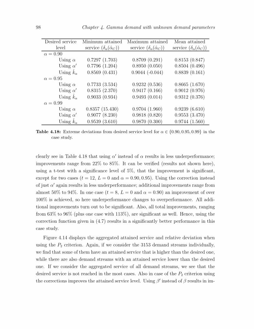
98 Chapter 4. Gamma demand with unknown demand parameters
Desired service Minimum attained Maximum attained Mean attainedlevel service (δα(αC)) service (δα(αC)) service (δα(αC))
α = 0.90Using α 0.7297 (1.703) 0.8709 (0.291) 0.8153 (0.847)Using α′ 0.7796 (1.204) 0.8950 (0.050) 0.8504 (0.496)
Using kα 0.8569 (0.431) 0.9044 (-0.044) 0.8839 (0.161)α = 0.95
Using α 0.7733 (3.534) 0.9232 (0.536) 0.8665 (1.670)Using α′ 0.8315 (2.370) 0.9417 (0.166) 0.9012 (0.976)
Using kα 0.9033 (0.934) 0.9493 (0.014) 0.9312 (0.376)α = 0.99
Using α 0.8357 (15.430) 0.9704 (1.960) 0.9239 (6.610)Using α′ 0.9077 (8.230) 0.9818 (0.820) 0.9553 (3.470)
Using kα 0.9539 (3.610) 0.9870 (0.300) 0.9744 (1.560)
Table 4.18: Extreme deviations from desired service level for α ∈ {0.90, 0.95, 0.99} in thecase study.
clearly see in Table 4.18 that using α′ instead of α results in less underperformance;
improvements range from 22% to 85%. It can be verified (results not shown here),
using a t-test with a significance level of 5%, that the improvement is significant,
except for two cases (t = 12, L = 0 and α = 0.90, 0.95). Using the correction instead
of just α′ again results in less underperformance; additional improvements range from
almost 50% to 94%. In one case (t = 8, L = 0 and α = 0.90) an improvement of over
100% is achieved, so here underperformance changes to overperformance. All addi-
tional improvements turn out to be significant. Also, all total improvements, ranging
from 63% to 96% (plus one case with 113%), are significant as well. Hence, using the
correction function given in (4.7) results in a significantly better performance in this
case study.
Figure 4.14 displays the aggregated attained service and relative deviation when
using the P2 criterion. Again, if we consider the 3153 demand streams individually,
we find that some of them have an attained service that is higher than the desired one,
while there are also demand streams with an attained service lower than the desired
one. If we consider the aggregated service of all demand streams, we see that the
desired service is not reached in the most cases. Also in case of the P2 criterion using
the corrections improves the attained service level. Using β ′ instead of β results in im-

4.4. Case study 99
tL
βC
β = 0.90
Using βUsing β ′
Using kβ
4
8
12
01
40.7
0.75
0.8
0.85
0.9
tL
δ β(β
C)
β = 0.90
Using βUsing β ′
Using kβ
4
8
12
01
4
0
0.5
1
1.5
2
tL
βC
β = 0.95
Using βUsing β ′
Using kβ
4
8
12
01
40.75
0.8
0.85
0.9
0.95
tL
δ β(β
C)
β = 0.95
Using βUsing β ′
Using kβ
4
8
12
01
4
0
1
2
3
4
tL
βC
β = 0.99
Using βUsing β ′
Using kβ
4
8
12
01
4
0.85
0.9
0.95
1
tL
δ β(β
C)
β = 0.99
Using βUsing β ′
Using kβ
4
8
12
01
4
0
5
10
15
Figure 4.14: Attained service (βC) and relative deviation (δβ(βC)) using the P2 criterionin the case study for.
provements ranging from almost 23% to 98%, plus one case (t = 8, L = 1, β = 0.90)
in which the desired service level is attained; the attained service level is 0.9004.

100 Chapter 4. Gamma demand with unknown demand parameters
Unfortunately, not all of these improvements are significant according to a t-test
with a significance level of 5%; 10 out of the 27 cases are not: all the cases at which
t = 12 plus the case at which t = 8, L = 4 and β = 0.90. If not only β ′ is used,
but also the correction function given in (4.9), additional improvements, ranging
from 2% up to 90% can be achieved in case the desired service level is not reached
completely. In four more cases the desired service level is reached: α = 0.90, 0.95,
t = 8, 12 and L = 0. Only if L = 4 and t = 4, t = 8 these improvements turn out to be
significant (for all the desired service levels). The total improvements range from 53%
to 95% for the 22 cases in which the desired service level is not reached completely,
and from 110% to 161% for the five cases in which the underperformance changes
to overperformance. If we consider the total improvements all of them, except for
t = 12, L = 1 and β = 0.90, 0.99, are significant. Hence we can state that using
the adapted desired service β ′ and the correction function, depending on β, together
improves the attained service level. Table 4.19 displays the extreme deviations.
Desired service Minimum attained Maximum attained Mean attained
level service (δβ(βC)) service (δβ(βC)) service (δβ(βC))β = 0.90
Using β 0.7705 (1.295) 0.8739 (0.261) 0.8288 (0.712)Using β ′ 0.8318 (0.682) 0.9004 (-0.004) 0.8648 (0.352)
Using kβ 0.8624 (0.376) 0.9184 (-0.184) 0.8915 (0.085)β = 0.95
Using β 0.8244 (2.512) 0.9290 (0.420) 0.8808 (1.384)Using β ′ 0.8836 (1.328) 0.9488 (0.024) 0.9147 (0.706)
Using kβ 0.9064 (0.872) 0.9585 (-0.170) 0.9354 (0.292)β = 0.99
Using β 0.8868 (10.320) 0.9762 (1.380) 0.9348 (5.520)Using β ′ 0.9353 (5.470) 0.9859 (0.410) 0.9608 (2.920)
Using kβ 0.9551 (3.490) 0.9887 (0.130) 0.9736 (1.640)
Table 4.19: Extreme deviations from desired service level for β ∈ {0.90, 0.95, 0.99} in thecase study.
We also did the case study calculations with a rolling horizon and the results are
similar; the significance results cannot be checked, since the outcomes on which the
attained service levels are based are no longer independent.

4.5. Summary results 101
4.5 Summary results
This chapter has considered the case of an (R, S) inventory control model with gamma
demand and a service criterion. It is shown that using estimates in the determination
of the order-up-to levels derived under the assumption that all parameters are known,
leads to underperformance. If demand is exponentially distributed and the lead time
is zero, it is shown that the desired service level is never reached. For the case of
the P1 criterion, Erlang demand, integer lead time and known shape parameter, we
have derived closed-form expressions for the attained service and use these to show
that the desired service is not met for higher values of α, i.e., α ≥ 0.50. For the
most realistic situation treated in this chapter (demand is truly gamma distributed
with unknown parameters) simulation is used to show that indeed underperformance
exists for both the P1 and P2 criterion and the desired service level set at 0.90 or
higher; these values are used in practice. Part of this underperformance could be
solved by using α′ instead of α for the P1 criterion (improvements range from 18% to
80%) and β ′ instead of β for the P2 criterion (improvements range from 16% to 99%
in case the desired service level is not met; it is met in 17 out of 180 cases).
Further improvements are obtained by applying a multiplicative correction to the
estimated order-up-to level. This correction is found using simulation and with help
of nested regression a function is constructed. Using the correction function causes
the attained service to reach the desired service even more closely. However, the
desired service level is not reached completely, due to the fact that the correction
functions are determined using the true value of ρ while in practice only ρ can be
used. The additional (total) improvements range from 60% to 99% (76% to 99%) for
the P1 criterion. The results for the additional improvements of the P2 criterion are
a bit more complicated, since in some cases the desired service level is (almost) met
without using the multiplicative correction. So in some cases the attained service
level declines a little, but in general the additional improvements are between a few
percent up to 94%. Total improvements range from 66% to 94%.
We also applied the corrections developed in this chapter to real demand data,
that was provided by Involvation and the Dutch Ministry of Defence. In case of
the P1 criterion the total improvements range from 63% to 96% and in one case the
desired service level is met. For the P2 criterion the total improvements range from
53% to 95% in the 22 cases in which the desired service level is not met; it is met
in the remaining 5 cases. This case study showed that, although our method has its

102 Chapter 4. Gamma demand with unknown demand parameters
limitations, it works well in practice.

Chapter 5
Mixed Erlang demand and randominventory control parameters
In this chapter the effect of randomness in the inventory control param-eters under mixed Erlang demand is discussed. For some industries, likeprocess industry, it is difficult to produce exactly the required replenish-ment quantity, due to, e.g., yield problems. Hence the optimal controlparameter is more a target than an exact result. We provide a method todeal with this uncertainty in inventory control by considering the controlparameters to be random, unlike classical inventory control. The methoddescribed in this chapter is for a periodic review, order-up-to policy (the(R, S) policy) under a service level constraint.
5.1 Introduction
Classical inventory theory assumes that demand can be stochastic, but that its dis-
tribution is known completely. Using that information it is possible to determine
the control parameter settings of a chosen reordering system to either minimize the
total costs or to reach a pre-specified service level. If the control parameters of the
reordering system are chosen, they will not change, and, assuming that the demand
is stationary, one can use these parameter settings, either to have minimal expected
cost or to reach the desired service level in the long run. This chapter considers the
effects that occur when these control parameters are random.
Chapters 3 and 4 treat the case that the demand parameters are random, which
results in the order-up-to level, one of the control parameters, being random. This
is not the only cause of randomness in the order-up-to level. Assume that indeed

104 Chapter 5. Mixed Erlang demand and random inventory control parameters
the demand distribution is completely known, so that the correct order-up-to level
can be determined. Due to certain circumstances the value of this order-up-to level
might not be attained exactly. One can think of manufacturing products: a certain
number of products fail quality tests and have to be repaired or even discarded. The
number of products that will be discarded is not exactly known beforehand, so there
is some uncertainty in the amount of products that will be available in order to satisfy
demand. This is often referred to as random yield; see Yano and Lee (1995) for a
review of literature of lot sizing under random yield. Another example, from process
industry, is the production of bacteria. It is possible to accurately aim the production
at a certain level, but occasionally a batch is contaminated and the whole batch has
to be destroyed.
The randomness of the length of the lead time is discussed in literature (see,
e.g., Kaplan, 1970, Chapter 7 of Zipkin, 2000, or Silver and Robb, 2008); uncertainty
in delivery times may be caused by, e.g., congestion, stock out at the supplier, or
weather conditions in case of sea transport.
However, the fact that the length of the review period may be random is less
present in literature. The source of this randomness might not be as intuitive com-
pared to the lead time: one simply states that the inventory position is reviewed at a
certain time interval, e.g., once a week, and then it is fixed. However, many chemical
companies do face randomness in the length of the review period. These companies
often have a cyclic production schedule: they produce products 1, . . . , n and then
start again with 1; see, e.g., Ashayeri et al. (2006). These cycles are also called cam-
paigns. In order to determine the optimal inventory level such that a certain desired
service level is attained, mostly an (R, S) or (R, s, S) policy is used; the latter implies
that the inventory position is reviewed every R units of time and is replenished up to
S if the inventory position is below s. The review of the inventory position typically
takes place at the start of the campaign. The length of the review period may be
exposed to variation, due to possible variation in the setup times or in the production
times for each of the products in the campaign.
This chapter does not focus on the cause of the uncertainty but considers the
consequences instead. In Chapters 3 and 4 the cause of the uncertainty of the order-
up-to level is used to find a first improvement of the attained service. In this chapter,
we do not only consider more control parameters being random (R and L are fixed
in earlier chapters), but we also include more causes for the randomness of S, so this
chapter is more general compared to Chapters 3 and 4.
5.2. Demand distribution and inventory policy 105
For reasons of flexibility in estimating demand and mathematical convenience, we
consider demand that follows a mixed Erlang distribution. Furthermore, we assume
that an (R, S) policy is used, subject to a service level constraint; P2 is considered.
The demand distribution and inventory policy are discussed in Section 5.2. Section
5.3 shows that if the length of the review period R and/or the lead time L and/or
the order-up-to level S are stochastic, the desired service level is not reached. Fur-
thermore, an easy algorithm to solve this problem is described and, under certain
conditions, the optimal order-up-to levels in case of random R, L, and S are found.
Section 5.4 concludes this chapter.
5.2 Demand distribution and inventory policy
This chapter considers four random elements in determining the correct (target)
order-up-to level:
1. Demand per period, with expected value E [D] and coefficient of variation CD;
2. Length of review period, with expected value E [R] = 1 and coefficient of vari-
ation CR;
3. Lead time, with expected value E [L] and coefficient of variation CL;
4. Order-up-to level, with expected value E [S] and coefficient of variation CS.
The first, stochastic demand, is treated extensively in literature (see, e.g., Silver et al.,
1998). This randomness is taken into account in all our calculations without elab-
orating on it. The remainder of this chapter discusses the three random elements
remaining explicitly and we refer to those as the three sources of randomness. In the
majority of the literature it is assumed that the length of the review period (in case
of a periodic review policy) and the length of the lead time are known and fixed.
Furthermore, it is assumed that the ordered amount will be received completely.
5.2.1 Inventory policy
We assume that an (R, S) inventory control policy with lead time L is used: each R
units of time an order is placed such that the inventory position is equal to the order-
up-to level S and that order is delivered L units of time later. This order-up-to level is
chosen such that the fraction of demand that can be satisfied immediately, is at least

106 Chapter 5. Mixed Erlang demand and random inventory control parameters
β. Demand that cannot be satisfied immediately, is backlogged. Mathematically, the
attained service is defined as
β = 1− E [(DR+L − S)+]− E [(DL − S)+]
E [DR], (5.1)
where DR+L (DL, DR) is demand during the review period plus lead time (lead time,
review period) and (x)+ = max(x, 0).
The possibility of R, L, and S being random implies that evaluating (5.1) could
be more difficult. An easy ‘solution’ to the problem created by randomness is to
assume that R and L are fixed and determine the order-up-to level using the expected
value. However, if we ignore the extra variability caused by R and L, we may expect
underperformance. Furthermore, also S may be random; if we ignore the randomness
of S and substitute S by E [S], we may expect additional underperformance (see
Chapters 3 and 4).
We still can use (5.1) to find the attained service level, but we need to take into
account that not only the demand per period is random, but also R, L and S are.
5.2.2 Demand distribution
Equation (5.1) is elaborated on while assuming mixed Erlang distributed demand
during the review period and during the lead time. If a variable X is mixed Erlang
distributed, its pdf (fζ(x)) is
fζ(x) = p1µk11
xk1−1
(k1 − 1)!e−µ1x + p2µ
k22
xk2−1
(k2 − 1)!e−µ2x,
where ζ is a vector containing the six demand parameters p1, p2, k1, k2, µ1, and µ2.
All parameters are nonnegative, p1 + p2 = 1, and k1, k2 ∈ N. The demand during
the review period has the demand parameters ζ = [p1, p2, k1, k2, µ1, µ2]; the demand
during lead time has the demand parameters η = [q1, q2, l1, l2, λ1, λ1].
Also the order-up-to level S is assumed to be mixed Erlang distributed, with
demand parameters ξ = [w1, w2, m1, m2, ρ1, ρ2].
Assuming that demand during review, demand during lead time, and the order-
up-to level can be accurately fitted to a mixed Erlang distribution with demand
parameters ζ, η, and ξ, respectively, we can determine two of the three expected
values in (5.1), namely E [DR] and E [(DL − S)+]:
E [DR] = p1k1µ1
+ p2k2µ2
, (5.2)

5.2. Demand distribution and inventory policy 107
E[(DL − S)+
]
S fixed=
2∑
j=1
qj
ljλj
lj∑
t=0
(λjS)t
t!e−λjS − S
lj−1∑
t=0
(λjS)t
t!e−λjS
, (5.3)
E[(DL − S)+
]
S random=
2∑
j=1
2∑
i=1
qjwi
lj∑
t=0
ρmi
i ljλt−1j (mi + t− 1)!
(mi − 1)!t!(λj + ρi)mi+t
−lj−1∑
t=0
ρmi
i λtj(mi + t)!
(mi − 1)!t!(λj + ρi)mi+t+1
. (5.4)
See Appendix E.2 for the derivation of (5.3) and (5.4).
We also need an expression for E [(DR+L − S)+]. If DR+L is mixed Erlang dis-
tributed, we would get similar expressions as in (5.3) and (5.4). However, the sum of
two mixed Erlang distributed variables is, in general, not mixed Erlang distributed.
The mixed Erlang distribution is a special case of the phase type distribution (see
Appendix E.3) and the sum of two phase type distributed variables has again a phase
type distribution. Hence, we know that DR+L is phase type distributed with demand
parameters τR+L and TR+L. If S is not assumed to be random, the expected amount
of backlog at the end of the replenishment cycle is
E[(DR+L − S)+
]=
∫ ∞
S
xfTR+L,τR+L(x)dx− S
(1− FTR+L,τR+L
(S)),
where fTR+L,τR+Ldenotes the pdf of a phase type distribution. If S is random, the
expected amount of backlog at the end of the replenishment cycle is
E[(DR+L − S)+
]=
∫ ∞
0
(∫ ∞
s
xfTR+L,τR+L(x)dx
)fξ(s)ds−
(w1
m1
ρ1+ w2
m2
ρ2
)
+
∫ ∞
0
sFTR+L,τR+L(s)fξ(s)ds,
with fξ the pdf of a mixed Erlang distribution with parameters ξ. The derivation of
these two expressions is in Appendix E.4, as are the algorithms needed to calculate
the pdf and cdf of the phase type distribution. Note that these expressions still have
integrals, which need to be numerically determined. This causes calculations to be
slow.

108 Chapter 5. Mixed Erlang demand and random inventory control parameters
5.2.3 Determining the order-up-to level
We find the distribution parameters in ζ, η, and ξ by assuming that we know the
first two moments of the demand per period (E [D] and CD), the length of the review
period (E [R] and CR) and the lead time (E [L] and CL). With help of those we can
determine the first two moments of the demand during review, and demand during
lead time:
E [Dℓ] = E [ℓ] · E [D] ℓ ∈ {R,L}C
2Dℓ
= C2D + C
2ℓ + C
2DC
2ℓ ℓ ∈ {R,L}.
Next, we can use (E.1) to find the parameters of the mixed Erlang distribution be-
longing to DR and DL. Further, we assume that the order-up-to level S has expected
value E [S] and coefficient of variation CS. If we fit a mixed Erlang distribution using
these first two moments using (E.1), the order-up-to level S has parameters ξ.
The attained backlogged demand is
E[(DR+L − S)+
]− E
[(DL − S)+
](5.5)
and the desired backlogged demand is
(1− β)E [DR] , (5.6)
where β is the desired service level. Note that (5.5) is decreasing in S, since the
higher the order-up-to level is, the lower the amount of backlogged demand will be.
If S is assumed to be deterministic, we can use binary search to find the value
for S such that (5.5) and (5.6) are equal. However, if we take possible randomness
of S into account, finding a value for S is not straightforward. In fact, we would
like to have values for E [S] and CS; having these values we should aim at realizing
these values in practice. However, it is not realistic that we can choose a value for
CS , since this value is a function of the production system itself. Being able to vary
the expected value does seem reasonable, since simply ordering a little more or a
little less will change the expected value. Hence, we decided to keep the coefficient of
variation fixed and only vary the expected value in the binary search. The resulted
expected value is then a target value for the order-up-to level instead of the value.

5.3. Validations and results 109
5.3 Validations and results
We have determined eight order-up-to levels for all combinations of different values
for the eight demand and control parameters listed in Table 5.1. The eight order-
Demand/control parameter Values usedE [D] 10, 20CD 0.25, 0.50, 0.75E [R] 1CR 0.25, 0.50, 0.75E [L] 0.5, 1, 2, 4CL 0.25, 0.50, 0.75CS 0, 0.25, 030, 0.35, 0.40, 0.45, 0.50, 0.55, 0.60β 0.90, 0.95
Table 5.1: Values used in simulation.
up-to levels take account of the randomness in various degrees. First, we assume no
randomness and the order-up-to level is denoted by Srls. The indices show the three
possible sources of randomness (length of review period, lead time and order-up-to
level, respectively). Lower case letters indicate no randomness assumed, while upper
case letters denote randomness. Next, we assume randomness in one of the three
sources; the three order-up-to levels are SrlS, SrLs and SRls. Then, two sources of
randomness are assumed; the order-up-to levels are SrLS, SRlS and SRLs. Finally, we
assume randomness in all three sources and this order-up-to level is SRLS .
The eight order-up-to levels are determined for all 3,888 combinations of de-
mand/control parameters listed in Table 5.1 as described in Section 5.2.3. The cor-
rectness of the computer program and formulae is checked using simulation. For each
of the 3, 888 combinations we generated n = 10, 000 times the demand during review
from a mixed Erlang distribution with parameters ζ, denoted by
diR, i = 1, . . . , n,
and 10, 000 times the demand during lead time from a mixed Erlang distribution
with parameters η, denoted by
diL, i = 1, . . . , n.
The demand during review plus lead time is the sum of these two:
diR+L = diR + diL, i = 1, . . . , n.
110 Chapter 5. Mixed Erlang demand and random inventory control parameters
Since S is assumed to be random for four of the order-up-to levels, also 10, 000 values
for each of SrlS, SrLS, SRlS, and SRLS need to be generated from a mixed Erlang
distribution with parameters ξ; denote these order-up-to levels by si,rlS, si,rLS, si,RlS,
and si,RLS. Note that si,rls = Srls, si,rLs = SrLs, si,Rls = SRls, and si,RLs = SRLs,
since there is no randomness in these order-up-to levels.
The simulated attained services βrls, . . . , βRLS for all eight order-up-to levels for
each combination are then determined using the n = 10, 000 demand observations:
βC = 1−1n
∑ni=1
((diR + diL − si,C)
+ − (diL − si,C)+
)
1n
∑ni=1 diR
, C ∈ {rls, . . . , RLS}.
We found that the simulated attained service levels are indeed very close to the
desired service levels; using a standard t-test with a significance level of 5% we find
that 95.07% of the 3, 888 · 8 = 31, 104 simulated attained service levels did not differ
significantly from the desired service level, so we can state that the (target) order-
up-to levels determined in the way described in Section 5.2.3 do result in reaching
the desired service level.
The remainder of this section considers the implications of adding the three
sources of randomness (length of review period, lead time, size of order-up-to level).
Beforehand, we expect that randomness in each of the variables will lead to a higher
(targeted) order-up-to level for the desired service level to be reached, since addi-
tional randomness causes variability in timing and quantities. Thus, in general, more
inventory is needed to be able to cope with this variability.
Figure 5.1 displays the eight (target) order-up-to levels for various values of CS and
the attained service when using Srls, SrlS, . . . , SRLS while all randomness is present.
First consider the left graph. The target order-up-to level is the expected value of
the order-up-to level when S is random. Note that if the order-up-to level is not
assumed to be random, CS does not have an effect on the order-up-to level, which
is logical. These order-up-to levels are depicted with the solid markers. Further,
comparing the two order-up-to levels for which only the randomness in S differs, e.g.,
SrLs (solid squares) and SrLS (open squares), one sees that the larger CS, the larger
the order-up-to level, as we expected. Figure 5.1 also shows that if one takes the
randomness of the length of the review period into account, while keeping the other
sources of randomness fixed, the order-up-to level increases; compare the lines with
the circles (R deterministic) to the lines with the diamonds (R random) and the lines
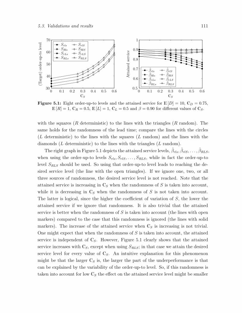
5.3. Validations and results 111
CS
(Target)
order-up-tolevel
Srls
SRls
SrLs
SRLs
SrlS
SRlS
SrLS
SRLS
0 0.1 0.2 0.3 0.4 0.5 0.630
40
50
60
70
CS
Attained
service
βrls
βRls
βrLs
βRLs
βrlS
βRlS
βrLS
βRLS
0 0.1 0.2 0.3 0.4 0.5 0.60.5
0.6
0.7
0.8
0.9
1
Figure 5.1: Eight order-up-to levels and the attained service for E [D] = 10, CD = 0.75,E [R] = 1, CR = 0.5, E [L] = 1, CL = 0.5 and β = 0.90 for different values of CS.
with the squares (R deterministic) to the lines with the triangles (R random). The
same holds for the randomness of the lead time; compare the lines with the circles
(L deterministic) to the lines with the squares (L random) and the lines with the
diamonds (L deterministic) to the lines with the triangles (L random).
The right graph in Figure 5.1 depicts the attained service levels, βrls, βrlS, . . . , βRLS,
when using the order-up-to levels Srls, SrlS, . . . , SRLS, while in fact the order-up-to
level SRLS should be used. So using that order-up-to level leads to reaching the de-
sired service level (the line with the open triangles). If we ignore one, two, or all
three sources of randomness, the desired service level is not reached. Note that the
attained service is increasing in CS when the randomness of S is taken into account,
while it is decreasing in CS when the randomness of S is not taken into account.
The latter is logical, since the higher the coefficient of variation of S, the lower the
attained service if we ignore that randomness. It is also trivial that the attained
service is better when the randomness of S is taken into account (the lines with open
markers) compared to the case that this randomness is ignored (the lines with solid
markers). The increase of the attained service when CS is increasing is not trivial.
One might expect that when the randomness of S is taken into account, the attained
service is independent of CS . However, Figure 5.1 clearly shows that the attained
service increases with CS, except when using SRLS; in that case we attain the desired
service level for every value of CS. An intuitive explanation for this phenomenon
might be that the larger CS is, the larger the part of the underperformance is that
can be explained by the variability of the order-up-to level. So, if this randomness is
taken into account for low CS the effect on the attained service level might be smaller

112 Chapter 5. Mixed Erlang demand and random inventory control parameters
than if it is taken into account for high CS.
These graphs can be made for all different combinations of E [D], CD, E [L], CL,
E [R], CR, and β. They all have similar characteristics (the more variability, the
higher the order-up-to level). However, the relative increase in the order-up-to level
differs among the different combinations. Figures 5.2 and 5.3 provide two examples.
Figure 5.2 displays a situation where the coefficient of variation of the length of the
CS
(Target)
order-up-tolevel
Srls
SRls
SrLs
SRLs
SrlS
SRlS
SrLS
SRLS
0 0.1 0.2 0.3 0.4 0.5 0.630
40
50
60
70
CS
Attained
service
βrls
βRls
βrLs
βRLs
βrlS
βRlS
βrLS
βRLS
0 0.1 0.2 0.3 0.4 0.5 0.60.5
0.6
0.7
0.8
0.9
1
Figure 5.2: Eight order-up-to levels and the attained service for E [D] = 10, CD = 0.75,E [R] = 1, CR = 0.25, E [L] = 1, CL = 0.75 and β = 0.90 for different values of CS.
review period is low compared to the coefficient of variation of the length of the
lead time. Comparing the lines for which only the randomness of R differs (circles
to diamonds and squares to triangles) one sees that those differences are smaller
than the differences between the lines for which the randomness of L differs (circles
to squares and diamonds to triangles). Figure 5.3 displays a situation where the
coefficient of variation of the length of the review period is high compared to the
coefficient of variation of the length of the lead time. Comparing the lines for which
only the randomness of R differs (circles to diamonds and squares to triangles) one
sees that those differences are larger than the differences between the lines for which
the randomness of L differs (circles to squares and diamonds to triangles).
Considering Figures 5.1–5.3, one clearly sees that ignoring randomness while it is
present leads to nonnegligible underperformance. In order to reach the desired service
level the target order-up-to level needs to be considerably larger, up to more than
twice as large. This implies that inventory level will increase considerably and that
means more inventory costs. Whether increasing inventory level (and thus inventory
costs) is justified by reaching the desired service level, is a subjective question, that
every inventory manager needs to answer for himself. However, the method described

5.4. Summary results 113
CS
(Target)
order-up-tolevel
Srls
SRls
SrLs
SRLs
SrlS
SRlS
SrLS
SRLS
0 0.1 0.2 0.3 0.4 0.5 0.630
40
50
60
70
80
CS
Attained
service
βrls
βRls
βrLs
βRLs
βrlS
βRlS
βrLS
βRLS
0 0.1 0.2 0.3 0.4 0.5 0.60.5
0.6
0.7
0.8
0.9
1
Figure 5.3: Eight order-up-to levels and the attained service for E [D] = 10, CD = 0.75,E [R] = 1, CR = 0.75, E [L] = 1, CL = 0.50 and β = 0.90 different values of CS .
in this chapter provides a tool for that inventory manager to make this decision.
Furthermore, it is often difficult to change the underlying reason of R, L and S being
random. However, seeing how much can be gained in terms of inventory costs, the
inventory manager might consider measures that seemed to be too expensive before.
He might consider using the supplier that is more expensive, but has a less variable
or even fixed lead time.
5.4 Summary results
This chapter has considered the effect of randomness in inventory control parameters.
In most literature it is assumed that control parameters are fixed, while in fact they
may be random. We have considered a periodic review, order-up-to level inventory
control policy (the (R, S) policy), which leads to three control parameters: the length
of the review period, the length of the lead time and the order-up-to level. A method
to take these three sources of randomness into account is provided while assuming
that the demand during the review period and demand during lead time is mixed
Erlang distributed. The order-up-to levels for 3888 combinations of demand and
control parameter values are determined, together with the attained service levels.
Simulation is used to validate the correctness of the order-up-to levels.
It is shown that not taking the randomness of the inventory control parameters
into account can lead to considerable underperformance. The figures in this chapter
show attained service levels below 0.70, while the desired service level is 0.90: an
underperformance of more than 20 percent points. The highest underperformance

114 Chapter 5. Mixed Erlang demand and random inventory control parameters
for all the 3888 combinations of demand and control parameters considered is 0.3659
(parameter setting E [D] = 10, CD = 0.25, E [R] = 1, CR = 0.75, E [L] = 1,
CL = 0.25, β = 0.95 and CS = 0.60).
Furthermore, the more randomness is taken into account and the more variable the
control parameters are, the higher the order-up-to level needs to be. This confirms our
a priori intuition and also is in line with the results of Chapters 3 and 4, in which we
showed that the more variable the order-up-to level, the larger the underperformance
is. We especially considered the randomness of the order-up-to level and showed with
graphs that the order-up-to level rapidly increases when the coefficient of variation
of the order-up-to level increases. This leads to higher inventory levels and, hence,
higher inventory costs. One could argue that it might be wiser to investigate the
source of the randomness thoroughly than to implement this method without a second
thought.
A second limitation on implementing this method directly is that it assumes that
the first two moments of demand, length of the review period, length of the lead time
and the height of the order-up-to level are known with certainty. However, in real
life, this will not be the case and we need to estimate them. This will probably again
lead to underperformance (see Chapters 3 and 4).
The main idea of this method, taking account of the randomness of the inventory
control parameters, has been applied to the inventory control in a big Dutch chemical
company, although it is not exactly as described in this chapter. In that case the
order-up-to level is assumed to follow a continuous uniform distribution, while de-
mand during review, lead time and review plus lead time is mixed Erlang distributed.
Using this approach has led to improving the inventory management of this company
considerably.

Chapter 6
Conclusions and future research
This chapter discusses overall results and conclusions. Also ideas for futureresearch are provided.
6.1 Conclusions
In the first part of this dissertation we construct a more flexible way to model demand
using two modified shifted gamma distributions. The first one, the modified shifted
gamma distribution with a point mass at zero, is constructed from a shifted gamma
distribution by setting all negative realizations to zero. This leads to the point mass
at zero, with probability of having a negative realization in the shifted gamma distri-
bution we start from. The second one, the truncated shifted gamma distribution, is
constructed from a shifted gamma distribution by ignoring all negative realizations.
Using these distributions leads to nice expressions for the order-up-to levels that are
easy to implement. Furthermore, the modified shifted gamma distribution with a
point mass at zero can directly be used to model intermittent demand, since the
possibility of having zero demand is not zero. Most commonly used demand distri-
butions do not have this property and, therefore, other approaches are used to model
intermittent demand. Furthermore, we prove that some results derived for both mod-
ified normal and modified gamma distributions hold in general. Finally, we show the
attained service when using a regular gamma distribution or a shifted gamma distri-
bution, while demand is actually modified shifted gamma distributed. We see that
the attained service does not differ largely from the desired service level; in some cases
it is a little below (maximal underperformance is 2.86 percent points) and in some
cases it is a little above (maximal overperformance is 2.37 percent points). Still, not

116 Chapter 6. Conclusions and future research
using the correct demand distribution does lead to not reaching the desired service
level and a deviation of 2.5 percent points can be too large, depending on the market
requirements.
The second part of this dissertation, Chapters 3–5, shows that not taking all ex-
isting randomness into account leads to serious underperformance. In Chapters 3 and
4 we focus on randomness in the order-up-to level that is caused by estimation of the
demand parameters. These estimates are based on historical demand observations.
The fewer the number of demand observations, the higher the variability in param-
eter estimates and hence the higher the variability in the order-up-to level, which is
a function of the demand parameters in most inventory control policies. Intuitively
this will lead to larger underperformance and it is shown that this indeed happens
in case of normal and gamma distributed demand, if the desired service level is rel-
atively large (at levels commonly used in practice). It is also shown that the larger
the variability in demand, the larger the underperformance, and that the larger the
desired service, the larger the relative underperformance. In Chapter 4 also lead time
is included and the larger the lead time, the larger the underperformance. None of
these results are counterintuitive.
Not only the existence and size of the underperformance is determined, also a
method to find an order-up-to level that leads to (almost) attaining the desired ser-
vice level is constructed. Both for the normal and gamma demand we analytically
derive a first improvement under strong assumptions (only mean demand unknown
in case of normal demand and exponential demand with zero lead time in case of
gamma demand). Next to that, we use a technique we call nested regression to con-
struct a correction function. In case of normal demand we find an additive correction
function, depending on the coefficient of variation, the number of historical demand
observations and the desired service level. If the true coefficient of variation is used,
the desired service level is indeed reached. However, in real life the coefficient of
variation needs to be estimated. Using this estimate leads to attaining the desired
service level with a deviation of at most 0.5 percent points. In case of gamma demand
we construct a multiplicative correction function depending on the coefficient of vari-
ation, the number of historical demand observations, the desired service level and
the lead time. Using this function with the true value of the coefficient of variation
leads to reaching the desired service level. If we use an estimate for the coefficient of
variation, the desired service level is not reached in all cases and especially in case of a
large coefficient of variation, the underperformance can still be substantial. However,

6.1. Conclusions 117
using the correction function together with the first improvement does improve the
attained service level significantly. The method of modeling demand according to a
gamma distribution and using the first improvement and the correction function is
applied to a case study. Not using any correction results in substantial underperfor-
mance, the first improvement increases the attained service, and using the correction
function as well leads to almost reaching the desired service level. Hence, the case
study shows that the method developed in Chapter 4 can also be used in practice.
The method for finding a correction to the order-up-to level as developed in Chap-
ters 3 and 4 can be used more general. If we have one output variable that depends
on multiple input variables and we use a full factorial design of the different values
of those input variables, nested linear regression (see Appendix B) can be used to
determine a function of the input variables that estimates the output variable. All
three correction functions in this dissertation (determined using nested linear regres-
sion) have high coefficients of determination; they are all more than 0.99. Hence, we
can state that the determined correction functions are very accurate in estimating
the correction needed.
Chapter 5 does not only consider randomness in the order-up-to level, but also
randomness in the other two inventory control parameters: length of the review pe-
riod and length of the lead time. Furthermore, we do not reflect on the cause of the
randomness in the three control parameters. This chapter studies the effect these
three sources of randomness have on attaining the desired service level in case of
mixed Erlang distributed demand during the review period and during the lead time
and a mixed Erlang distributed order-up-to level. We have chosen the mixed Er-
lang distribution, since it is a flexible distribution that is mathematically tractable
as well. We show analytically that ignoring the randomness leads, again, to substan-
tial underperformance. Taking the randomness of the three control parameters into
account leads to reaching the desired service level at the expense of high order-up-to
levels, which result in high inventory costs. Hence, it could be wiser to try reducing
the randomness than to mindlessly implement the new order-up-to levels. One could
reduce the randomness in several ways, e.g., by choosing a more expensive but more
reliable supplier to decrease the randomness in the lead time, or investing in new
production equipment, which leads to less rejected products, hence less randomness
in the order-up-to level. Also investing in a better forecast method could help, since
also forecasting (estimation of the demand parameters) leads to randomness in the
order-up-to level, as discussed in Chapters 3 and 4.

118 Chapter 6. Conclusions and future research
6.2 Ideas for future research
In this dissertation we consider the (R, S) inventory control policy, because of the
relative easy derivation of the order-up-to levels. One main idea for future research
is considering other inventory control policies. We expect to see similar results, es-
pecially regarding Part II: if randomness in the control parameters is not taking into
account, the desired service level will not be reached and substantial underperfor-
mance arises.
Furthermore, in this dissertation we are interested in the attained service in the
long run. In case of the cycle service criterion, it does not make a difference whether
we consider the attained service over a finite horizon or whether we consider the long
run attained service, but in case of the fill rate the expected attained service over
a finite horizon can be shown to be higher than the long run attained service, see
Thomas (2005). It might be interesting to study the attained service over a finite
horizon in the case of unknown demand and control parameters, especially in the
light of the assumption of a finite number of historical demand observations.
Chapter 2 considers two modified shifted gamma distributions to model demand
in a setting with zero lead time. The work in this chapter is inspired by the work of
Strijbosch and Moors (2006), who also assume zero lead time. It is already argued
that zero lead time might seem very rigid, but that it could occur in practice, e.g.,
a supermarket could order after opening hours and that order is delivered the next
morning before the supermarket opens again. However, the lead time will be posi-
tive in general and therefore one could expand the work done in Chapter 2 and in
Strijbosch and Moors (2006) by including the possibility of a positive lead time.
One of the advantages of using the modified shifted gamma distribution with a
point mass at zero is that it can be used to model intermittent demand. We have
not elaborated on that in this dissertation; it is an idea for future research, including
comparing using the modified shifted gamma distribution with a point mass at zero
to using a compound distribution to model intermittent demand, e.g., the compound
Bernoulli distribution, as described in Janssen et al. (1998).
Furthermore, in this chapter it is assumed that all demand parameters are known
with certainty, while in practice this will not be the case. Hence, the demand pa-
rameters need to be estimated, for example by using the first three moments of the
modified gamma distributions. In Chapters 3 and 4 we have seen that estimation of
the demand parameters leads to underperformance, and, therefore, we expect that

6.2. Ideas for future research 119
this will also occur in case of the modified gamma distributions. This is an interesting
idea to elaborate on.
First shifting the gamma distribution and using this shifted gamma distribution
to construct the modified shifted gamma distribution might be a little artificial, but
the shifted gamma distribution can be used in the context of inventory management,
albeit a little different compared to the use in this thesis. One could think of an
inventory model in which the distribution of the forecast errors plays a role. One
makes a forecast of the demand and the error belonging to that forecast can be either
positive, when demand is higher than forecasted, or negative, when demand is lower
than forecasted. The lowest demand possible is zero, so the forecast error can never
be smaller than minus the forecast. In this situation the shifted gamma distribution
arises naturally, since the forecast error can become infinitely large, but is bounded
from below. The location parameter of the shifted gamma distribution (∆) should
be taken equal to the forecasted demand. So, if one would have an inventory model
that needs the distribution of the forecast error as an input, using the shifted gamma
distribution would be an interesting idea.
Part II considers the effect of randomness in the inventory control parameters, as-
suming that demand is stationary. In real life situations the demand pattern changes
over time. A first study on the influence of forecasting on inventory control in case
of non-stationary demand is performed by Strijbosch et al. (2010), which is accepted
for publication. This is a very interesting topic to study further.
In Chapters 3 and 4 we consider sample statistics and the first two moments of
the normal and gamma distribution to estimate demand during the review period
and during the lead time. This is a very simple method of estimating demand (also
known as (simple) moving average in forecasting), and is used in this dissertation be-
cause of the tractable results. There are more sophisticated methods to estimate or
forecast demand. One widely used method is exponential smoothing; in this method
the more recent demand observations are more important than the older demand
observations and therefore it will react faster to changing demand patterns. Also
exponential smoothing leads to tractable results and therefore most of the analytical
derivations in this dissertation could also be performed with parameters that are es-
timated using exponential smoothing. Furthermore, we could also use more complex
forecasting methods, e.g., ARIMA. If the method is calibrated in a good way, this will
probably result in less underperformance. However, it is not likely that we will find
any analytical results when using complex forecasting methods. Finally, we could

120 Chapter 6. Conclusions and future research
also use maximum likelihood estimation to estimate the parameters. Unfortunately,
this could lead to intractable results, depending on the distribution we want to fit
on the historical demand observations. We could, of course, use simulation to find
whether the maximum likelihood estimators lead to less underperformance.
In Chapters 3 and 4 correction functions are derived that depend, amongst others,
on the coefficient of variation of demand. This is in both correction functions the
only input variable that we do not know. Therefore, we estimate the coefficient of
variation using the estimates for the mean and standard deviation. This estimate
is not unbiased (the estimate of the standard deviation is not unbiased; see also
Section 3.3.2), and therefore it is hard to believe that this is the best estimate for the
coefficient of variation. Finding a better one could help in improving the attained
service even further.
The correction functions in Chapters 3 and 4 are constructed using a technique
we call nested linear regression. Of course, there are other methods known to esti-
mate function prescriptions based on a set of values for input and output variables.
Comparing these other methods to nested linear regression is an interesting idea to
follow up.
In Chapter 3 the lead time is assumed to be zero. Zero lead time might not
be unrealistic, but in most cases lead times will be positive. Hence, considering
the possibility of non-zero (deterministic) lead time is a logical addition. We expect
results analogous to Chapter 4, where non-zero lead time is considered. So, intuitively
we expect to find that the larger the lead time, the lower the attained service and
that the correction function needs to depend on the lead time, next to the coefficient
of variation, the number of historical demand observations and the desired service
level.
We could also include a random lead time in the situations described in Chapters
3 and 4. This will probably lead to even lower attained service levels if this random-
ness is ignored, as seen in Chapter 5. If it is taken into account, it will probably
result in another input variable in the correction function, the coefficient of varia-
tion in the lead time, which needs to be estimated. It will complicate the analysis
of these situations (normally distributed demand and gamma distributed demand)
even further and probably no tractable results will exist, unless strict assumptions
are made. However, since random lead times often appear in real life and the normal
distribution is widely used (also the gamma distribution is used in practice), it will
be a useful extension to the work as presented in Chapters 3 and 4.

6.2. Ideas for future research 121
The derivations in Chapter 5 are quite theoretical: we assume that we do know
the means and coefficients of variation of demand, the length of the review period, the
length of the lead time and the order-up-to level in order to show that randomness in
the three control parameters leads to underperformance if ignored. In practice, we do
not know these means and coefficients of variation with certainty, and we would need
to estimate them using historical observations, probably leading again to even more
underperformance. This model becomes very complex if we would like to include
all unknown demand and control parameters and, therefore, tractable results cannot
be expected. However, using simulation we could find the influences of all random
elements in the model. Furthermore, if we make the ideas discussed in Chapter 5
more applicable in practice, we can do a comparison study of the three methods
discussed in Chapters 3–5 and find which distribution, i.e., normal, gamma or mixed
Erlang, is best to assume in different situations.
The three methods discussed in Chapters 3–5 all assume a continuous demand
distribution, which implies that demand occurs in every review period (the probability
of having zero demand is zero in a continuous distribution). However, a lot of types of
products will have an intermittent demand pattern. If the possibility of zero demand
is small or even negligible, then using a continuous demand distribution will not lead
to large under- or overperformance. If this probability is not small, then we should use
another method to estimate demand. One possibility is using the truncated normal
distribution or truncated shifted gamma distribution, as discussed in Chapter 2.
Another possibility is using a compound distribution. In both methods we need to
estimate demand parameters and this estimation leads to variability in the order-up-
to level. Since intermittent demand is essentially different from continuous demand,
this does not necessarily lead to large underperformance and, hence, studying this
situation might lead to interesting results and insights.
This dissertation is mainly about the effects of randomness in the demand and
control parameters on the attained service. We have seen that these effects can be
quite large and therefore the randomness cannot be ignored. Methods are provided
to deal with the uncertainty in demand parameters, i.e., the correction functions con-
structed in Chapters 3 and 4. A really distribution-free approach can be found using
robust optimization. In practice, one does not know the demand distribution and
therefore assumes a distribution, e.g., the normal or gamma distribution. Not using
the true distribution could lead to not reaching the desired service level (see Chap-
ter 2), but whether under- or overperformance will occur, is not known beforehand;

122 Chapter 6. Conclusions and future research
note that both under- and overperformance are undesirable. If a distribution-free
approach is used, one does not have the problem of choosing a good distribution.
Applying robust optimization to inventory control is a relative new field of research.
The main idea is using historical demand observations and a goodness-of-fit test to
determine robust control parameters that can deal with uncertainty in demand and
in the demand distribution. This might lead to an elegant solution to the problems
that arise from the randomness in the demand and control parameters.

Appendix A
Derivations Chapter 2
A.1 Derivation of equations (2.1) and (2.2)
Let fρ,θ(x) and Fρ,θ(x) denote the pdf and cdf of the regular gamma distribution and
fρ,θ,∆(x) and Fρ,θ,∆(x) the pdf and cdf of the shifted gamma distribution. We know
that
∫ ∞
x
(z − x)fρ,θ(z)dz = ρθ[1− Fρ+1,θ(x)]− x[1− Fρ,θ(x)],
xfρ,θ(x) = θρfρ+1,θ(x).
We can rewrite these equations to the shifted gamma distribution using that fρ,θ,∆(x) =
fρ,θ(x+∆) and Fρ,θ,∆(x) = Fρ,θ(x+∆) (or fρ,θ,∆(x−∆) = fρ,θ(x) and Fρ,θ,∆(x−∆) =
Fρ,θ(x)):
∫ ∞
w
(y − w)fρ,θ(y)dy = ρθ[1− Fρ+1,θ(w)]− w[1− Fρ,θ(w)],
∫ ∞
w
(y − w)fρ,θ,∆(y −∆)dy = ρθ[1− Fρ+1,θ,∆(w −∆)]− w[1− Fρ,θ,∆(w −∆)],
Substitute z = y −∆, y = z +∆, dy = dz (since dydz
= 1),∫ ∞
w−∆
(z +∆− w)fρ,θ,∆(z)dz = ρθ[1− Fρ+1,θ,∆(w −∆)]− w[1− Fρ,θ,∆(w −∆)],
Substitute x = w −∆, w = x+∆,∫ ∞
x
(z − x)fρ,θ,∆(z)dz = ρθ[1− Fρ+1,θ,∆(x)]− (x+∆)[1− Fρ,θ,∆(x)],

124 Appendix A. Derivations Chapter 2
(x+∆)fρ,θ(x+∆) = θρfρ+1,θ(x+∆),
(x+∆)fρ,θ,∆(x) = θρfρ+1,θ,∆(x),
xfρ,θ,∆(x) = θρfρ+1,θ,∆(x)−∆fρ,θ,∆(x). (A.1)
In one of the derivations in Chapter 2 we need to rewrite x2fρ,θ,∆(x); we can obtain
that result by first multiplying both the left-hand side and right-hand side of (A.1)
by x and then applying (A.1) to the right-hand side:
x · (xfρ,θ,∆(x)) = x ·(θρfρ+1,θ,∆(x)−∆fρ,θ,∆(x)
)(A.2)
= θρxfρ+1,θ,∆(x)−∆xfρ,θ,∆(x),
x2fρ,θ,∆(x) = θρ[θ(ρ+ 1)fρ+2,θ,∆(x)−∆fρ+1,θ,∆(x)]
−∆[θρfρ+1,θ,∆(x)−∆fρ,θ,∆(x)],
x2fρ,θ,∆(x) = θ2ρ(ρ+ 1)fρ+2,θ,∆(x)− 2∆θρfρ+1,θ,∆(x) + ∆2fρ,θ,∆(x). (A.3)
In another derivation in Chapter 2 we need to rewrite x3fρ,θ,∆(x); we can obtain that
result by first multiplying both the left-hand side and right-hand side of (A.3) by x
and then applying (A.1) to the right-hand side:
x · (x2fρ,θ,∆(x)) = x ·(θ2ρ(ρ+ 1)fρ+2,θ,∆(x)− 2∆θρfρ+1,θ,∆(x) + ∆2fρ,θ,∆(x)
),
x3fρ,θ,∆(x) = θ2ρ(ρ+ 1)xfρ+2,θ,∆(x)− 2∆θρxfρ+1,θ,∆(x) + ∆2xfρ,θ,∆(x)
= θ2ρ(ρ+ 1)(θ(ρ+ 2)fρ+3,θ,∆(x)−∆fρ+2,θ,∆(x)
)
− 2∆θρ(θ(ρ+ 1)fρ+2,θ,∆(x)−∆fρ+1,θ,∆(x)
)
+∆2(θρfρ+1,θ,∆(x)−∆fρ,θ,∆(x)
)
= θ3ρ(ρ+ 1)(ρ+ 2)fρ+3,θ,∆(x)− 3∆θ2ρ(ρ+ 1)fρ+2,θ,∆(x)
+ 3∆2θρfρ+1,θ,∆(x)−∆3fρ,θ,∆(x).
A.2 First three moments of shifted gamma distri-
bution
In this section we derive the first three moments of the shifted gamma distribution
and use these to write the three demand parameters as a function of the first three
moments. If X is distributed according to a regular gamma distribution with param-
eters ρ and θ (the shifted gamma distribution with ρ, θ, and ∆ = 0), the kth moment
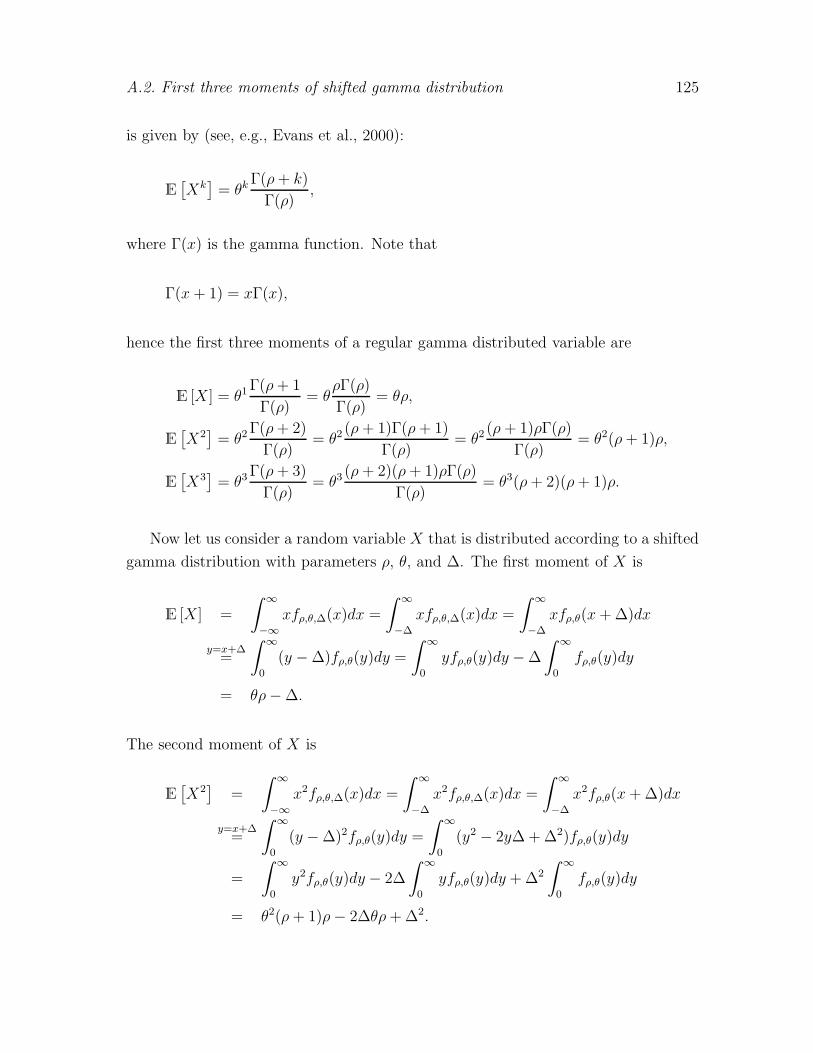
A.2. First three moments of shifted gamma distribution 125
is given by (see, e.g., Evans et al., 2000):
E[Xk]= θk
Γ(ρ+ k)
Γ(ρ),
where Γ(x) is the gamma function. Note that
Γ(x+ 1) = xΓ(x),
hence the first three moments of a regular gamma distributed variable are
E [X ] = θ1Γ(ρ+ 1
Γ(ρ)= θ
ρΓ(ρ)
Γ(ρ)= θρ,
E[X2]= θ2
Γ(ρ+ 2)
Γ(ρ)= θ2
(ρ+ 1)Γ(ρ+ 1)
Γ(ρ)= θ2
(ρ+ 1)ρΓ(ρ)
Γ(ρ)= θ2(ρ+ 1)ρ,
E[X3]= θ3
Γ(ρ+ 3)
Γ(ρ)= θ3
(ρ+ 2)(ρ+ 1)ρΓ(ρ)
Γ(ρ)= θ3(ρ+ 2)(ρ+ 1)ρ.
Now let us consider a random variable X that is distributed according to a shifted
gamma distribution with parameters ρ, θ, and ∆. The first moment of X is
E [X ] =
∫ ∞
−∞xfρ,θ,∆(x)dx =
∫ ∞
−∆
xfρ,θ,∆(x)dx =
∫ ∞
−∆
xfρ,θ(x+∆)dx
y=x+∆=
∫ ∞
0
(y −∆)fρ,θ(y)dy =
∫ ∞
0
yfρ,θ(y)dy −∆
∫ ∞
0
fρ,θ(y)dy
= θρ−∆.
The second moment of X is
E[X2]
=
∫ ∞
−∞x2fρ,θ,∆(x)dx =
∫ ∞
−∆
x2fρ,θ,∆(x)dx =
∫ ∞
−∆
x2fρ,θ(x+∆)dx
y=x+∆=
∫ ∞
0
(y −∆)2fρ,θ(y)dy =
∫ ∞
0
(y2 − 2y∆+∆2)fρ,θ(y)dy
=
∫ ∞
0
y2fρ,θ(y)dy − 2∆
∫ ∞
0
yfρ,θ(y)dy +∆2
∫ ∞
0
fρ,θ(y)dy
= θ2(ρ+ 1)ρ− 2∆θρ+∆2.

126 Appendix A. Derivations Chapter 2
The third moment of X is
E[X3]
=
∫ ∞
−∞x3fρ,θ,∆(x)dx =
∫ ∞
−∆
x3fρ,θ,∆(x)dx =
∫ ∞
−∆
x3fρ,θ(x+∆)dx
y=x+∆=
∫ ∞
0
(y −∆)3fρ,θ(y)dy =
∫ ∞
0
(y3 − 3y2∆+ 3y∆2 −∆3)fρ,θ(y)dy
=
∫ ∞
0
y3fρ,θ(y)dy − 3∆
∫ ∞
0
y2fρ,θ(y)dy + 3∆2
∫ ∞
0
yfρ,θ(y)dy
−∆3
∫ ∞
0
yfρ,θ(y)dy
= θ3(ρ+ 2)(ρ+ 1)ρ− 3∆θ2(ρ+ 1)ρ+ 3∆2θρ−∆3.
Let us denote the first, second and third moment by µ, µ2 and µ3, so we have:
µ = θρ−∆,
µ2 = θ2ρ2 + θ2ρ− 2∆θρ+∆2,
µ3 = θ3ρ3 + 3θ3ρ2 + 2θ3ρ− 3∆θ2ρ2 − 3∆θ2ρ+ 3∆2θρ−∆3.
We now have these three moments as functions of the demand parameters ρ, θ
and ∆; it could be useful to have the demand parameters as functions of µ, µ2 and µ3
(see 2.5). With a little rewriting we can obtain such functions. First, let us consider
µ:
µ = ρθ −∆ ⇒ θρ = µ+∆ ⇒ ρ =µ+∆
θ.
Next, substitute all ρ in the expression for µ2 by µ+∆θ
(or, equivalently, all θρ by
µ+∆):
µ2 = (µ+∆)2 + θ(µ+∆)− 2∆(µ+∆) +∆2
= µ2 + 2µ∆+∆2 + θµ+ θ∆− 2µ∆− 2∆2 +∆2
= θµ+ θ∆+ µ2.
Analogously for the expression of µ3:
µ3 = (µ+∆)3 + 3θ(µ+∆)2 + 2θ2(µ+∆)
− 3∆(µ+∆)2 − 3∆θ(µ+∆) + 3∆2(µ+∆)−∆3
= µ3 + 3µ2∆+ 3µ∆2 +∆3 + 3θµ2 + 6θµ∆+ 3θ∆2 + 2θ2µ+ 2θ2∆
− 3∆µ2 − 6µ∆2 − 3∆3 − 3∆θµ− 3θ∆2 + 3∆2µ+ 3∆3 −∆3
= µ3 + 3θµ2 + 2θ2µ+ 3θµ∆+ 2θ2∆.

A.2. First three moments of shifted gamma distribution 127
Now we can rewrite µ2:
µ2 = θµ+ θ∆+ µ2 ⇒ θ∆ = µ2 − µ2 − θµ
⇒ ∆ =µ2 − µ2 − θµ
θ=
µ2 − µ2
θ− µ.
Note that we can use this to rewrite the expression for ρ:
ρ =µ+ µ2−µ2
θ− µ
θ=
µ2 − µ2
θ2=
σ2
θ2.
Also substitute ∆ = µ2−µ2
θ− µ in the expression for µ3:
µ3 = µ3 + 3θµ2 + 2θ2µ+ 3θµ(
µ2−µ2
θ− µ
)+ 2θ2
(µ2−µ2
θ− µ
)
= µ3 + 3θµ2 + 2θ2µ+ 3µµ2 − 3µ3 − 3θµ2 + 2θµ2 − 2θµ2 − 2θ2µ
= −2µ3 + 3µµ2 + 2θµ2 − 2θµ2 = −2µ3 + 3µµ2 + 2θ(µ2 − µ2).
Rewriting this last equation provides an expression of θ that solely depends on the
first three moments of X :
2θ(µ2 − µ2) = µ3 + 2µ3 − 3µµ2 ⇒ θ =µ3 + 2µ3 − 3µµ2
2(µ2 − µ2).
The expressions for ∆ and ρ follow easily when θ is substituted with the expression
above:
∆ = (µ2 − µ2)2(µ2 − µ2)
µ3 + 2µ3 − 3µµ2=
2(µ2 − µ2)2
µ3 + 2µ3 − 3µµ2,
ρ = (µ2 − µ2)
(2(µ2 − µ2)
µ3 + 2µ3 − 3µµ2
)2
=4(µ2 − µ2)3
(µ3 + 2µ3 − 3µµ2)2.


Appendix B
Nested linear regression
Nested regression is used in Chapters 3 and 4 to estimate a correction function for
the order-up-to level. To our knowledge, Strijbosch and Moors (1999) are the first to
use this technique. The method is explained in this appendix.
We start with a dependent variable Y that depends on n independent variables
X1, X2, . . . , Xn. The different values of the independent variables (denoted by Xi)
form a full factorial design, so every combination of different values of X1, X2, . . . , Xn
exists.
Example B.1 (Full factorial design)
The sets of possible values of X1, X2 and X3 are X1 = {10, 20, 30}, X2 = {0.90, 0.95}and X3 = {0.4, 0.8}. So there are 3 · 2 · 2 = 12 combinations of X1, X2, X3 for which
a value of Y is known, i.e., the combinations:
X1 X2 X3 X1 X2 X3 X1 X2 X3
10 0.90 0.4 20 0.90 0.4 30 0.90 0.410 0.90 0.8 20 0.90 0.8 30 0.90 0.810 0.95 0.4 20 0.95 0.4 30 0.95 0.410 0.95 0.8 20 0.95 0.8 30 0.95 0.8
�
The estimation process has n steps and in each of the steps one independent variable
is chosen to be regressed on Y (in the first step) or on the estimated coefficients of
the previous step. The regression is repeated for all combinations of the values of the
variables that are not chosen that step or any of the previous steps. The estimated
coefficients therefore depend on the non-chosen variables and this dependency is used
in the following step(s). We follow this complicated procedure, since we want to have

130 Appendix B. Nested linear regression
the possibility to choose a power to which the chosen independent variable is raised.
Below the steps are described in more detail. In this description we choose X1
in the first step, X2 in the second step, X3 in the third, etcetera, but of course any
order of choosing the independent variables is possible. Furthermore, let Xi denote
the vector [Xi, Xi+1, . . . , Xn]′ and X denote [X1, X2, . . . , Xn]
′.
Step 1 For every combination of values of X2, . . . , Xn the value of Y is estimated
depending on X1. We assume that the relation has the following form:
Y (X) = γ0(r,X2) + γ1(r,X2)Xr1 + ε.
Note that the coefficients depend on the non-chosen variables and on the power to
which X1 is raised. If we would not have a constant (γ0), we could use logarithms to
find the value of r with help of linear regression, but this is not possible in the current
form. Therefore, the coefficients are estimated for a set of values of r (denoted by
R), and the value for which the sum of squared errors (SSE for short) is minimized is
chosen. For each value of r a regression equation Y (r,X) = g0(r,X2) + g1(r,X2)Xr1
is estimated. Then the best value of r, denoted by r, is found by solving
r = argminr∈R∑
X1∈X1
∑
X2∈X2
· · ·∑
Xn∈Xn
(Y (X)− Y (r,X)
)2.
Step 2 In this step the coefficients g0 and g1 are regressed on the independent
variable X2 for each of the combinations of X3, . . . , Xn. The relations are supposed
to have the following form:
g0 = γ00(r0,X3) + γ01(r0,X3)Xr02 + ε,
g1 = γ10(r1,X3) + γ11(r1,X3)Xr12 + ε.
For each value of r0 and r1 a regression equation gi(ri,X2) = gi0(ri,X3)+gi1(ri,X3)Xri2
(i ∈ {0, 1}) is estimated and the best values for r0 and r1 are found by minimizing
the SSE:
r0 = argminr0∈R∑
X2∈X2
· · ·∑
Xn∈Xn
(g0(X2)− g0(r0,X2))2 ,
r1 = argminr1∈R∑
X2∈X2
· · ·∑
Xn∈Xn
(g1(X2)− g1(r1,X2))2 .

B. Nested linear regression 131
Step 3 In this step the coefficients gij (i, j ∈ {0, 1}) are regressed on the inde-
pendent variable X3 for each of the combinations of X4, . . . , Xn. The relations are
supposed to have the following form:
gij = γij0(rij ,X4) + γij1(rij,X4)Xrij3 + ε.
For each value of rij a regression equation gij(rij,X3) = gij0(rij,X4)+gij1(rij ,X4)Xrij3
is estimated and the best values for rij are found by minimizing the SSE:
rij = argminrij∈R∑
X3∈X3
· · ·∑
Xn∈Xn
(gij(X3)− gij(rij,X3))2 .
These steps are repeated in a similar way until the last step n.
Step n In the previous step coefficients gi1,...,in−1(i1, . . . , in−1 ∈ {0, 1}) were esti-
mated. In this last step we apply linear regression one more time. The relations are
supposed to have the following form:
gi1,...,in−1= γi1,...,in−10(ri1,...,in−1
) + γi1,...,in−11(ri1,...,in−1)X
ri1,...,in−1
n + ε.
For each value of ri1,...,in−1a regression equation is estimated, resulting in gi1,...,in−1
=
gi1,...,in−10(ri1,...,in−1) + gi1,...,in−11(ri1,...,in−1
)Xri1,...,in−1
n and the values for ri1,...,in−1are
chosen such that the SSE is minimized:
ri1,...,in−1= argminri1,...,in−1
∈R∑
Xn∈Xn
(gi1,...,in−1
(Xn)− gi1,...,in−1(ri1,...,in−1
, Xn))2
.
Finally, the estimates for the coefficients are substituted in each other and we
obtain a formula which can be used to estimate Y , depending on X1, . . . , Xn:
Y = g0 + g1Xr1
=(g00 + g01X
r02
)+(g10 + g11X
r12
)Xr
1
=((
g000 + g001Xr003
)+(g010 + g011X
r013
)Xr0
2
)
+((
g100 + g101Xr103
)+(g110 + g111X
r113
)Xr1
2
)Xr
1
= . . .
In order to clarify this procedure we will show how we estimated (3.15).

132 Appendix B. Nested linear regression
Example B.2 (Nested regression)
In Section 3.3.4 we try to find a good formula for the correction needed to attain the
desired service level, denoted by ks. This correction depends on ν, t and β (in the
calculations we use 1− β). We will first choose ν, then t and finally β.
Step 1 In the first step ν is regressed on ks. The relation is assumed to have the
following form:
ks(ν, t, β) = γ0(r, t, β) + γ1(r, t, β)νr + ε. (B.1)
Figure B.1 displays the relation between ν and ks for three different combinations
of t and β. It shows that the assumed relation seems to fit quite well to the actual
ks(ν, 4, 0.90)
ks(ν, 4, 0.95)
ks(ν, 10, 0.95)
ν
ks
0.1 0.2 0.3 0.4 0.5 0.6 0.7 0.8 0.9-0.1
0
0.1
0.2
0.3
0.4
0.5
0.6
0.7
0.8
0.9
Figure B.1: ks (ν, t, β) for some values of t and β.
situation; the value of r probably is close to 1.
In order to find a good value for r, regression (for each combination of t and β)
is performed for values of r ranging from −20 to 20 in steps of 0.01 (0 is excluded),
resulting in a regression equation ks(r, ν, t, β) = g0(r, t, β) + g1(r, t, β)νr. We need
to perform these regressions for every value of r because the form in (B.1) does not
allow to estimate values for γ0, γ1, and r in one regression step. Further, we cannot
decide on a good value for r a priori, hence we use a greedy approach to find it. The

B. Nested linear regression 133
sum of squared errors (SSE) is determined for each value of r according to
SSE(r) =∑
ν∈V
∑
t∈T
∑
β∈B(ks(ν, t, β)− ks(r, ν, t, β))
2,
where V, T and B are the sets of values for ν, t and β (see also (3.12)). The value of r
is chosen such that the SSE is minimized. Figure B.2 shows the SSE depending on
r. The value of r for which the SSE is lowest, is r = 0.90. The estimated coefficients
r
SSE(r)
-20 -15 -10 -5 0 5 10 15 200
100
200
300
400
500
600
700
800
Figure B.2: SSE(r) depending on the exponent r.
g0 and g1 for every combination of t and β are listed in Tables B.1 and B.2.
β = 0.90 β = 0.91 β = 0.92 β = 0.93 β = 0.94 β = 0.95 β = 0.96 β = 0.97 β = 0.98 β = 0.99t = 2 −1.252 −0.835 −0.687 −0.560 −0.528 −0.520 −0.532 −0.481 −0.480 −0.483t = 3 0.435 0.054 −0.043 −0.100 −0.144 −0.159 −0.154 −0.171 −0.179 −0.177t = 4 0.273 0.077 −0.005 −0.041 −0.057 −0.083 −0.080 −0.077 −0.087 −0.085t = 5 0.199 0.068 0.004 −0.010 −0.021 −0.033 −0.040 −0.042 −0.044 −0.043t = 6 0.157 0.063 0.023 0.010 −0.007 −0.012 −0.017 −0.021 −0.025 −0.023t = 7 0.148 0.059 0.034 0.023 −0.001 −0.002 −0.015 −0.014 −0.014 −0.013t = 8 0.149 0.067 0.035 0.025 0.009 0.000 −0.004 −0.007 −0.011 −0.010t = 10 0.127 0.065 0.040 0.015 0.012 0.001 0.002 −0.008 −0.007 −0.005t = 12 0.093 0.056 0.034 0.022 0.002 −0.002 0.000 −0.007 −0.005 −0.001t = 15 0.077 0.047 0.024 0.012 0.009 0.008 0.004 −0.003 −0.003 −0.006t = 20 0.060 0.034 0.021 0.015 0.004 0.006 −0.001 −0.005 −0.007 −0.001
Table B.1: Estimated values for γ0.

134 Appendix B. Nested linear regression
β = 0.90 β = 0.91 β = 0.92 β = 0.93 β = 0.94 β = 0.95 β = 0.96 β = 0.97 β = 0.98 β = 0.99t = 2 28.812 14.135 9.298 6.758 5.299 4.421 3.815 3.209 2.856 2.564t = 3 4.323 2.963 2.238 1.851 1.583 1.356 1.165 1.065 0.965 0.859t = 4 2.082 1.488 1.168 0.975 0.810 0.717 0.619 0.535 0.481 0.422t = 5 1.309 0.922 0.748 0.590 0.492 0.424 0.370 0.324 0.284 0.249t = 6 0.913 0.626 0.500 0.394 0.339 0.284 0.242 0.209 0.185 0.153t = 7 0.659 0.478 0.356 0.281 0.253 0.206 0.179 0.158 0.128 0.105t = 8 0.472 0.352 0.277 0.212 0.187 0.158 0.133 0.115 0.099 0.080t = 10 0.306 0.223 0.178 0.152 0.117 0.114 0.082 0.087 0.072 0.053t = 12 0.252 0.164 0.125 0.103 0.108 0.090 0.070 0.067 0.058 0.032t = 15 0.184 0.115 0.096 0.087 0.065 0.052 0.042 0.043 0.038 0.030t = 20 0.117 0.085 0.063 0.047 0.053 0.034 0.036 0.037 0.031 0.017
Table B.2: Estimated values for γ1.
So, for example, if we know that t = 4 and β = 0.90, the correction is estimated to
be
0.273 + 2.082ν0.90.
Note that, although the results in both tables are rounded to three decimals, we have
used the unrounded results for the following step.
Step 2 In this step we will regress t on the estimated coefficients of Step 1 for every
value of β. We assume the relations
g0(r0, β) = γ00(r0, β) + γ01(r0, β)tr0 + ε,
g1(r1, β) = γ10(r0, β) + γ11(r0, β)tr1 + ε.
If we consider β = 0.90, then we take all g0 for which β = 0.90 and regress tr0 on
those values. The value of r0 is chosen in the same way as in Step 1, i.e., we find
the value of r for which the SSE is minimized. This value is r0 = −9.17. In the
same way we estimate γ10, γ11, and the best value for r1, which is r1 = −4.19. The
values of g00, g01, g10, and g11 are listed in Table B.3. If we know that β = 0.90, the
correction, depending on ν and t, is estimated to be
(−0.035− 259.665t−9.17) + (0.124 + 45.646t−4.19)ν0.90.
Again, the results in this table are rounded to three decimals; we have used the
unrounded results for the final step.
Step 3 In the last step β is regressed on the four sets of coefficients found in step
2. Actually, we have chosen to use (1 − β) as an independent variable, since this is

B. Nested linear regression 135
g00 g01 g10 g11β = 0.90 −0.035 −259.665 0.124 45.646β = 0.91 −0.037 −257.118 0.150 50.630β = 0.92 −0.034 −259.279 0.170 56.782β = 0.93 −0.029 −291.183 0.183 67.574β = 0.94 −0.026 −286.663 0.215 78.252β = 0.95 −0.018 −295.662 0.248 93.834β = 0.96 −0.001 −323.357 0.277 119.946β = 0.97 0.019 −406.928 0.314 165.327β = 0.98 0.061 −516.219 0.351 252.385β = 0.99 0.175 −817.650 0.288 517.293
Table B.3: Estimated values for γ00, γ01, γ10, and γ11.
used in the determination of the safety factor cτβ; see (3.11). The following relations
are assumed:
g00(r00, β) = γ000(r00) + γ001(r00)(1− β)r00 + ε,
g01(r01, β) = γ010(r01) + γ011(r01)(1− β)r01 + ε,
g10(r10, β) = γ100(r10) + γ101(r10)(1− β)r10 + ε,
g11(r11, β) = γ110(r11) + γ111(r11)(1− β)r11 + ε.
The coefficients and values of r00, r01, r10, and r11 are estimated in the same way as
before. The best values for the powers are r00 = −0.95, r01 = −1.00, r10 = 1.41 and
r11 = −1.03; the obtained estimates g000, g001, . . . , g111 are in Table B.4. The final
g000 g001 g010 g011 g100 g101 g110 g111−0.0669 0.00305 −185.124 −6.359 0.335 −5.671 −3.481 4.541
Table B.4: The estimates for the coefficients γ000, . . . , γ111.
formula for estimating the correction needed is now given by
ks(ν, t, β) =[ (−0.0669 + 0.00305(1− β)−0.95
)+(−185.124− 6.359(1− β)−1.00
)t−9.17
]
+[ (
0.335− 5.671(1− β)1.41)+(−3.481 + 4.541(1− β)−1.03
)t−4.19
]ν0.90.
�


Appendix C
Derivations Chapter 3
C.1 Independence of achieved performance of µ
and σ
This appendix shows that the achieved performance depends on the quotient of σ
and µ (and thus on the coefficient of variation ν), but that it is independent of
µ and σ separately. Three order-up-to levels, S(dt, stτ, cτβ), S(dt, stτ, c
τβ) and S(dt +
κi (νt, t, β) st, stτ, cτβ), are considered. The first is discussed in Section 3.3.2, the second
in Section 3.3.3 and the third in Section 3.3.4. Remember that (x)+ = max(0, x).
C.1.1 S(dt, stτ, cτβ)
The service achieved in simulation is denoted by β (Sn), where Sn is the vector of
the n order-up-to levels determined for the n samples. It is defined as
β (Sn) = 1−∑n
j=1 (dj − Sj)+
∑nj=1 dj
.
In this definition dj denotes the observation that is used to check the order-up-to
level obtained in the j-th simulation run (n runs in total). Sj = S(dtj , stjτ, cτβ) is the
order-up-to level determined in the j-th simulation, where dtj and stj are defined as
dtj =1t
t∑
i=1
dij and stj =
√√√√ 1t−1
t∑
i=1
(dij − dtj
)2.
In the above d1j, . . . , dtj are the t demand observations that are used in the j-th
simulation run to determine the order-up-to level.

138 Appendix C. Derivations Chapter 3
Since dj ∼ N(µ, σ2), d∗j =dj−µ
σ∼ N(0, 1) and hence d∗j is indeed independent of
µ and σ. Note that the same holds for d∗ij = (dij − µ)/σ. Also S∗j = (Sj − µ)/σ is
independent of µ and σ:
S∗j =
1t
∑ti=1 dij + stjc
τβτ − µ
σ=
1
t
t∑
i=1
((dij − µ
σ
)+(stjσ
)cτβτ
)
=1
t
t∑
i=1
d∗ij + s∗tjcτβτ.
In the above s∗tj = stj/σ. It suffices to show that s∗tj is independent of µ and σ:
s∗tj =stjσ
=
√1
t−1
∑ti=1
(dij − 1
t
∑ti=1 dij
)2
σ
=
√√√√ 1t−1
t∑
i=1
(dij − µ
σ− 1
t
t∑
i=1
dij − µ
σ
)2
=
√√√√ 1t−1
t∑
i=1
(d∗ij − 1
t
t∑
i=1
d∗ij
)2
.
Note that dj = d∗jσ+µ and Sj = S∗j σ+µ. If these are substituted in the definition
for the simulated performance, we obtain
β (Sn) = 1−1n
∑nj=1
(d∗jσ + µ−
(S∗jσ + µ
))+1n
∑nj=1 d
∗jσ + µ
= 1−1n
∑nj=1 σ
(d∗j − S∗
j
)+1n
∑nj=1 d
∗jσ + µ
= 1−1n
∑nj=1
(d∗j − S∗
j
)+1n
∑nj=1 d
∗j + ν−1
.
Thus the performance only consists of terms independent of µ and σ. It does, however,
clearly depend on ν: directly through ν−1 in the denominator and indirectly through
cτβ in S∗j .
C.1.2 S(dt, stτ, cτβ)
The only thing that changes with respect to the previous section is that now ν has
to be estimated (else cτβ cannot be found). Using the same line of reasoning results
in s∗t = st/σ and d∗t = (dt − µ)/σ being both independent of µ and σ. So νt = st/dt
is independent of µ and σ:
νt =stdt
=s∗tσ
d∗tσ + µ=
s∗td∗t + ν−1
.

C.1. Independence of achieved performance of µ and σ 139
As stated before cτβ is defined as
cτβ =
{G−1
(1−βνtτ
)if νt > 0,
− 1νtτ
otherwise.
Thus both for νt > 0 and νt ≤ 0, cτβ purely depends on terms independent of µ and
σ. Hence, cτβ is independent of µ and σ and it is already shown that the other terms
in (S(dt, stτ, cτβ) − µ)/σ are. Hence the performance will again be independent of µ
and σ.
C.1.3 S(dt + κi (νt, t, β) st, stτ, cτβ)
So again (S(dt + κi (νt, t, β) st, stτ cτβ)− µ)/σ (i ∈ {σ, s}) should be independent of µ
and σ. This order-up-to level can be rewritten as
S(dt + κi (νt, t, β) st, cτβ) = S(dt, stτ, c
τβ) + κi (νt, t, β) st.
Hence it suffices to show that κi (νt, t, β) st/σ is independent of µ and σ. This is
easily seen, if one realizes that νt and st/σ are independent of µ and σ. Thus the
performance of this order-up-to level is independent of µ and σ.


Appendix D
Derivations Chapter 4
D.1 The attained service level in simulation
n : Number of simulations;i : Simulation run (i = 1, . . . , n);diR : Demand during review in ith run;diL : Demand during lead time in ith run;si : Estimated order-up-to level in ith run;I(c) : Indicator function: 1 if c is true and 0 otherwise.
In case of a P1 criterion the attained service level (αj, j ∈ {1, 2, 3, 4}) is determined
by
αj =
∑ni=1 I(si > diR + diL)
n.
In case of a P2 criterion the attained service level (βj , j ∈ {0, 1, 2, 3, 4}) is determined
by
βj = 1−∑n
i=1
[(diR + diL − si)
+ − (diL − si)+]
∑ni=1 diR
.
D.2 Equality order-up-to levels under P1 and P2
if demand is exponential
Remember that in case of the P1 criterion the order-up-to level S satisfied the equality
P (D1+L > S) = 1−α or P(D∗
1+L > S∗) = 1−α, where S∗ = 1θS. Let us now consider

142 Appendix D. Derivations Chapter 4
the service equality in case of a P2 criterion. Choose S such that it satisfies
E[(D1+L − S)+
]− E
[(DL − S)+
]= (1− β)E [D]
⇔ θ(E[(D∗
1+L − S∗)+]− E
[(D∗
L − S∗)+])
= (1− β)θ
⇔ E[(D∗
1+L − S∗)+]− E
[(D∗
L − S∗)+]= 1− β. (D.1)
Note that, analogously to the P1 case, D∗ℓ = 1
θDℓ ∼ Γ(ℓ, 1) and S∗ = 1
θS. Since it
is assumed that the desired service levels under the P1 and P2 policy are chosen to
be equal, we have α = β. Hence, the right hand sides of both service equations are
equal, so if the left hand sides of the service equations are equal as well, then S∗ = S∗
or S = S. So consider the left hand side of (D.1). Note that rf1+r,1(x) = xfr,1(x)
and F1+r,1(x) = Fr,1(x)− f1+r,1(x). We obtain that
E[(D∗
1+L − S∗)+]− E
[(D∗
L − S∗)+]
= L1+L,1(S∗)−LL,1(S
∗)
= (1 + L)[1− F2+L,1(S∗)]− S∗[1− F1+L(S
∗)]− LL,1(S∗)
= (1 + L)[1− F1+L,1(S∗) + f2+L(S
∗)]
− S∗[1− FL(S∗) + f1+L(S
∗)]− LL,1(S∗)
= (1 + L)[1− F1+L,1(S∗)]− S∗[1− FL(S
∗)] (D.2)
+ (1 + L)f2+L(S∗)− S∗f1+L(S
∗)−LL,1(S∗)
= 1− F1+L,1(S∗) + LL,1(S
∗) + S∗f1+L(S∗)− S∗f1+L(S
∗)− LL,1(S∗)
= 1− F1+L,1(S∗) = P
(D∗
1+L > S∗) .
Thus, the left hand sides of the service equations are equal as well and therefore the
order-up-to levels under the P1 and P2 criterion will be equal if demand is exponen-
tially distributed.
D.3 Simulation results
The tables below display the results of the calculations and simulations for figures
and tables with extreme values in Chapter 4.

D.3. Simulation results 143
α = 0.90 α = 0.95 α = 0.99L ρ t = 4 t = 8 t = 12 t = 4 t = 8 t = 12 t = 4 t = 8 t = 120 1
30.8158 0.8572 0.8714 0.8681 0.9094 0.9232 0.9269 0.9621 0.9726
4413
0.8541 0.8761 0.8839 0.9102 0.9299 0.9366 0.9682 0.9801 0.983716517
0.8624 0.8804 0.8868 0.9184 0.9340 0.9393 0.9743 0.9828 0.98531 1
30.7696 0.8304 0.8527 0.8238 0.8850 0.9066 0.8910 0.9453 0.9623
4413
0.8261 0.8600 0.8726 0.8846 0.9161 0.9272 0.9516 0.9727 0.979016517
0.8370 0.8659 0.8766 0.8956 0.9218 0.9310 0.9605 0.9766 0.98154 1
30.6935 0.7783 0.8138 0.7470 0.8353 0.8708 0.8220 0.9070 0.9374
4413
0.7702 0.8229 0.8452 0.8293 0.8821 0.9031 0.9083 0.9510 0.965316517
0.7841 0.8311 0.8510 0.8437 0.8903 0.9088 0.9219 0.9576 0.96956 1
30.6635 0.7542 0.7944 0.7153 0.8113 0.8523 0.7910 0.8866 0.9232
4413
0.7450 0.8037 0.8300 0.8028 0.8634 0.8891 0.8844 0.9373 0.956316517
0.7596 0.8127 0.8366 0.8181 0.8726 0.8955 0.8996 0.9452 0.9613
Table D.1: Attained service level for Figure 4.2.

144 Appendix D. Derivations Chapter 4
α = 0.90 α = 0.95 α = 0.99L ρ t = 4 t = 8 t = 12 t = 4 t = 8 t = 12 t = 4 t = 8 t = 120 1
20.7991 0.8447 0.8606 0.8445 0.8933 0.9112 0.9000 0.9485 0.9638
1 0.8054 0.8494 0.8662 0.8567 0.9023 0.9171 0.9169 0.9564 0.96814413
0.8196 0.8594 0.8730 0.8718 0.9103 0.9236 0.9299 0.9649 0.97346 0.8238 0.8615 0.8731 0.8746 0.9114 0.9262 0.9312 0.9657 0.97499 0.8264 0.8620 0.8756 0.8781 0.9142 0.9264 0.9333 0.9659 0.9761
1 12
0.7483 0.8146 0.8400 0.7959 0.8676 0.8924 0.8592 0.9270 0.94991 0.7670 0.8256 0.8507 0.8169 0.8826 0.9010 0.8862 0.9413 0.95964413
0.7917 0.8410 0.8604 0.8437 0.8959 0.9138 0.9082 0.9533 0.96756 0.7967 0.8468 0.8637 0.8508 0.8992 0.9173 0.9120 0.9568 0.96929 0.8015 0.8480 0.8650 0.8533 0.9030 0.9178 0.9156 0.9581 0.9705
413
12
0.6685 0.7554 0.7975 0.7142 0.8118 0.8525 0.7855 0.8822 0.92001 0.6993 0.7776 0.8097 0.7477 0.8327 0.8688 0.8216 0.9050 0.93534413
0.7357 0.8016 0.8295 0.7869 0.8586 0.8850 0.8586 0.9255 0.94876 0.7419 0.8088 0.8346 0.7946 0.8645 0.8878 0.8685 0.9307 0.95269 0.7484 0.8101 0.8365 0.7993 0.8671 0.8912 0.8714 0.9339 0.9551
6 12
0.6449 0.7405 0.7818 0.6911 0.7894 0.8370 0.7579 0.8653 0.90721 0.6785 0.7611 0.7982 0.7291 0.8159 0.8570 0.8014 0.8912 0.92554413
0.7165 0.7872 0.8153 0.7656 0.8411 0.8727 0.8378 0.9152 0.94116 0.7255 0.7942 0.8203 0.7753 0.8490 0.8794 0.8484 0.9192 0.94489 0.7332 0.7970 0.8243 0.7834 0.8527 0.8819 0.8518 0.9246 0.9470
9 12
0.6144 0.7106 0.7599 0.6575 0.7658 0.8132 0.7244 0.8375 0.88771 0.6497 0.7353 0.7761 0.6970 0.7880 0.8332 0.7675 0.8677 0.90914413
0.6924 0.7634 0.7992 0.7367 0.8184 0.8552 0.8110 0.8952 0.92616 0.7030 0.7698 0.8062 0.7483 0.8272 0.8609 0.8210 0.9022 0.93219 0.7063 0.7745 0.8073 0.7563 0.8302 0.8633 0.8276 0.9050 0.9339
Table D.2: Attained service level for Figure 4.3.

D.3. Simulation results 145
α = 0.90 α = 0.95 α = 0.99L ρ t = 4 t = 8 t = 12 t = 4 t = 8 t = 12 t = 4 t = 8 t = 120 1
20.8515 0.8740 0.8811 0.8989 0.9211 0.9302 0.9534 0.9711 0.9769
1 0.8632 0.8802 0.8870 0.9141 0.9305 0.9360 0.9651 0.9774 0.98064413
0.8768 0.8905 0.8942 0.9260 0.9383 0.9425 0.9731 0.9833 0.98556 0.8802 0.8919 0.8941 0.9280 0.9397 0.9449 0.9742 0.9837 0.98659 0.8824 0.8929 0.8968 0.9312 0.9419 0.9453 0.9746 0.9843 0.9865
1 12
0.8032 0.8454 0.8608 0.8553 0.8988 0.9127 0.9249 0.9549 0.96611 0.8266 0.8570 0.8721 0.8801 0.9134 0.9218 0.9471 0.9677 0.97474413
0.8517 0.8730 0.8819 0.9037 0.9265 0.9338 0.9624 0.9761 0.98126 0.8571 0.8786 0.8857 0.9099 0.9288 0.9370 0.9641 0.9779 0.98239 0.8593 0.8799 0.8864 0.9114 0.9329 0.9375 0.9655 0.9792 0.9834
413
12
0.7220 0.7860 0.8190 0.7787 0.8467 0.8759 0.8678 0.9197 0.94211 0.7568 0.8095 0.8323 0.8162 0.8679 0.8919 0.9021 0.9403 0.95614413
0.7940 0.8350 0.8524 0.8532 0.8929 0.9083 0.9305 0.9570 0.96796 0.8005 0.8420 0.8567 0.8613 0.8990 0.9108 0.9374 0.9616 0.96999 0.8070 0.8429 0.8590 0.8641 0.9010 0.9129 0.9399 0.9634 0.9729
6 12
0.6964 0.7705 0.8030 0.7554 0.8253 0.8605 0.8445 0.9053 0.93191 0.7328 0.7933 0.8201 0.7960 0.8523 0.8800 0.8861 0.9302 0.94764413
0.7736 0.8196 0.8377 0.8344 0.8772 0.8975 0.9160 0.9504 0.96176 0.7834 0.8268 0.8430 0.8426 0.8842 0.9026 0.9236 0.9532 0.96529 0.7913 0.8295 0.8466 0.8491 0.8880 0.9053 0.9253 0.9571 0.9658
9 12
0.6624 0.7400 0.7807 0.7197 0.8005 0.8374 0.8134 0.8811 0.91451 0.7032 0.7660 0.7986 0.7623 0.8251 0.8581 0.8571 0.9087 0.93454413
0.7492 0.7951 0.8208 0.8032 0.8541 0.8795 0.8949 0.9335 0.94946 0.7583 0.8027 0.8286 0.8172 0.8628 0.8847 0.9025 0.9403 0.95499 0.7639 0.8066 0.8299 0.8240 0.8656 0.8880 0.9086 0.9422 0.9561
Table D.3: Attained service level for Figure 4.4.

146 Appendix D. Derivations Chapter 4
α = 0.90 α = 0.95 α = 0.99L ρ t = 4 t = 8 t = 12 t = 4 t = 8 t = 12 t = 4 t = 8 t = 120 1
20.8826 0.8935 0.8961 0.9290 0.9414 0.9446 0.9756 0.9836 0.9861
1 0.8883 0.8949 0.8976 0.9373 0.9449 0.9467 0.9804 0.9857 0.98704413
0.8924 0.8982 0.8995 0.9417 0.9464 0.9486 0.9841 0.9881 0.98866 0.8938 0.8975 0.8977 0.9419 0.9461 0.9493 0.9858 0.9881 0.98939 0.8956 0.8977 0.8998 0.9464 0.9485 0.9493 0.9877 0.9887 0.9893
1 12
0.8654 0.8876 0.8924 0.9149 0.9365 0.9414 0.9676 0.9789 0.98401 0.8767 0.8913 0.8974 0.9247 0.9416 0.9436 0.9744 0.9833 0.98554413
0.8868 0.8952 0.8991 0.9357 0.9467 0.9475 0.9806 0.9861 0.98816 0.8898 0.8984 0.9008 0.9393 0.9457 0.9498 0.9836 0.9874 0.98859 0.8915 0.8995 0.9002 0.9414 0.9487 0.9498 0.9856 0.9884 0.9896
413
12
0.8434 0.8730 0.8878 0.8953 0.9254 0.9347 0.9543 0.9743 0.97961 0.8616 0.8834 0.8898 0.9103 0.9301 0.9399 0.9634 0.9789 0.98274413
0.8746 0.8911 0.8953 0.9226 0.9406 0.9428 0.9721 0.9830 0.98666 0.8785 0.8957 0.8979 0.9274 0.9418 0.9443 0.9767 0.9848 0.98619 0.8840 0.8967 0.9001 0.9303 0.9442 0.9458 0.9791 0.9860 0.9882
6 12
0.8399 0.8757 0.8849 0.8916 0.9222 0.9343 0.9508 0.9722 0.97891 0.8575 0.8831 0.8894 0.9081 0.9305 0.9393 0.9615 0.9776 0.98224413
0.8733 0.8910 0.8941 0.9203 0.9378 0.9434 0.9696 0.9829 0.98506 0.8782 0.8943 0.8975 0.9245 0.9399 0.9447 0.9737 0.9840 0.98639 0.8865 0.8970 0.8992 0.9309 0.9434 0.9462 0.9760 0.9857 0.9870
9 12
0.8387 0.8734 0.8854 0.8899 0.9221 0.9335 0.9479 0.9709 0.97781 0.8587 0.8818 0.8895 0.9055 0.9295 0.9368 0.9587 0.9763 0.98194413
0.8747 0.8905 0.8955 0.9161 0.9368 0.9421 0.9658 0.9805 0.98446 0.8809 0.8957 0.9008 0.9228 0.9414 0.9436 0.9683 0.9842 0.98639 0.8872 0.8990 0.9034 0.9292 0.9436 0.9467 0.9730 0.9850 0.9877
Table D.4: Attained service level for Figure 4.6.

D.3. Simulation results 147
α = 0.90 α = 0.95 α = 0.99L ρ t = 4 t = 8 t = 12 t = 4 t = 8 t = 12 t = 4 t = 8 t = 120 1
20.9014 0.9006 0.8992 0.9490 0.9502 0.9493 0.9895 0.9900 0.9897
1 0.9002 0.8988 0.8994 0.9504 0.9499 0.9492 0.9901 0.9897 0.98934413
0.8988 0.8999 0.9005 0.9486 0.9487 0.9497 0.9891 0.9899 0.98976 0.8979 0.8991 0.8985 0.9478 0.9479 0.9502 0.9895 0.9893 0.99009 0.8991 0.8985 0.9000 0.9504 0.9498 0.9501 0.9902 0.9898 0.9898
1 12
0.8998 0.9009 0.8996 0.9482 0.9507 0.9497 0.9895 0.9897 0.98971 0.8991 0.8993 0.9016 0.9492 0.9501 0.9484 0.9901 0.9894 0.98934413
0.8993 0.8994 0.9009 0.9496 0.9511 0.9499 0.9894 0.9894 0.98966 0.9001 0.9011 0.9022 0.9502 0.9496 0.9515 0.9900 0.9897 0.98989 0.9000 0.9017 0.9016 0.9506 0.9515 0.9516 0.9903 0.9903 0.9908
413
12
0.8992 0.8984 0.9023 0.9494 0.9500 0.9501 0.9895 0.9898 0.99001 0.8998 0.8988 0.8982 0.9488 0.9473 0.9494 0.9904 0.9895 0.98944413
0.8972 0.9000 0.9003 0.9473 0.9490 0.9476 0.9889 0.9889 0.98976 0.8972 0.9013 0.9016 0.9475 0.9486 0.9479 0.9897 0.9893 0.98909 0.9005 0.9022 0.9024 0.9473 0.9503 0.9492 0.9901 0.9898 0.9903
6 12
0.9044 0.9031 0.9029 0.9509 0.9508 0.9522 0.9895 0.9903 0.99031 0.9023 0.9008 0.8997 0.9516 0.9487 0.9502 0.9909 0.9900 0.98964413
0.9007 0.9008 0.8996 0.9484 0.9484 0.9488 0.9891 0.9897 0.98936 0.8992 0.9022 0.9012 0.9483 0.9485 0.9489 0.9893 0.9895 0.98949 0.9047 0.9034 0.9025 0.9504 0.9505 0.9499 0.9892 0.9903 0.9895
9 12
0.9109 0.9082 0.9077 0.9556 0.9544 0.9545 0.9909 0.9910 0.99061 0.9109 0.9051 0.9033 0.9550 0.9523 0.9500 0.9919 0.9906 0.99094413
0.9079 0.9025 0.9022 0.9498 0.9486 0.9493 0.9899 0.9891 0.98906 0.9063 0.9060 0.9058 0.9505 0.9510 0.9493 0.9886 0.9906 0.98979 0.9086 0.9071 0.9077 0.9526 0.9515 0.9516 0.9893 0.9904 0.9906
Table D.5: All attained service levels for Table 4.10.

148 Appendix D. Derivations Chapter 4
β = 0.90 β = 0.95 β = 0.99L ρ t = 4 t = 8 t = 12 t = 4 t = 8 t = 12 t = 4 t = 8 t = 120 1
20.7950 0.8463 0.8605 0.8515 0.9009 0.9180 0.9188 0.9589 0.9714
1 0.8393 0.8663 0.8798 0.8919 0.9215 0.9315 0.9536 0.9731 0.97864413
0.8715 0.8852 0.8910 0.9237 0.9364 0.9420 0.9748 0.9837 0.98576 0.8792 0.8895 0.8926 0.9305 0.9396 0.9443 0.9791 0.9849 0.98709 0.8835 0.8911 0.8942 0.9346 0.9421 0.9451 0.9811 0.9857 0.9873
1 12
0.7662 0.8264 0.8456 0.8209 0.8855 0.9026 0.8934 0.9448 0.96251 0.8024 0.8485 0.8659 0.8596 0.9048 0.9185 0.9306 0.9622 0.97384413
0.8408 0.8675 0.8789 0.8973 0.9231 0.9319 0.9595 0.9750 0.98086 0.8522 0.8742 0.8835 0.9074 0.9279 0.9359 0.9658 0.9793 0.98299 0.8583 0.8788 0.8855 0.9130 0.9332 0.9379 0.9702 0.9810 0.9841
413
12
0.7029 0.7776 0.8168 0.7558 0.8383 0.8718 0.8313 0.9108 0.93981 0.7339 0.8011 0.8286 0.7938 0.8591 0.8868 0.8729 0.9319 0.95354413
0.7741 0.8256 0.8476 0.8329 0.8858 0.9050 0.9110 0.9515 0.96636 0.7836 0.8341 0.8532 0.8447 0.8932 0.9089 0.9223 0.9578 0.96829 0.7937 0.8383 0.8566 0.8510 0.8972 0.9124 0.9299 0.9616 0.9719
6 12
0.6778 0.7646 0.8000 0.7331 0.8161 0.8587 0.8098 0.8977 0.93221 0.7121 0.7842 0.8118 0.7699 0.8435 0.8770 0.8536 0.9196 0.94534413
0.7518 0.8104 0.8325 0.8082 0.8690 0.8927 0.8896 0.9422 0.95886 0.7632 0.8179 0.8386 0.8216 0.8770 0.8987 0.9035 0.9478 0.96279 0.7743 0.8225 0.8438 0.8316 0.8818 0.9025 0.9078 0.9526 0.9649
9 12
0.6491 0.7376 0.7789 0.6987 0.7957 0.8362 0.7794 0.8698 0.91211 0.6823 0.7596 0.7934 0.7381 0.8151 0.8538 0.8190 0.8973 0.93064413
0.7250 0.7828 0.8143 0.7760 0.8426 0.8736 0.8595 0.9225 0.94496 0.7368 0.7926 0.8226 0.7893 0.8533 0.8797 0.8717 0.9309 0.95089 0.7414 0.7967 0.8253 0.7993 0.8566 0.8835 0.8787 0.9335 0.9531
Table D.6: Attained service level for Figure 4.7.

D.3. Simulation results 149
β = 0.90 β = 0.95 β = 0.99L ρ t = 4 t = 8 t = 12 t = 4 t = 8 t = 12 t = 4 t = 8 t = 120 1
20.7078 0.7853 0.8154 0.7648 0.8455 0.8759 0.8448 0.9192 0.9441
1 0.7803 0.8291 0.8526 0.8340 0.8885 0.9076 0.9024 0.9479 0.96144413
0.8457 0.8714 0.8810 0.8941 0.9200 0.9306 0.9475 0.9710 0.97716 0.8629 0.8807 0.8866 0.9094 0.9284 0.9366 0.9573 0.9750 0.98069 0.8723 0.8850 0.8903 0.9187 0.9337 0.9394 0.9636 0.9776 0.9820
1 12
0.6905 0.7760 0.8047 0.7411 0.8342 0.8642 0.8187 0.9033 0.93341 0.7468 0.8141 0.8404 0.8006 0.8707 0.8928 0.8751 0.9335 0.95394413
0.8080 0.8487 0.8657 0.8596 0.9033 0.9179 0.9219 0.9579 0.97036 0.8272 0.8608 0.8741 0.8789 0.9123 0.9254 0.9351 0.9654 0.97419 0.8395 0.8687 0.8785 0.8892 0.9209 0.9294 0.9445 0.9698 0.9773
413
12
0.6408 0.7334 0.7830 0.6868 0.7924 0.8354 0.7587 0.8662 0.90631 0.6878 0.7693 0.8037 0.7390 0.8246 0.8622 0.8150 0.9001 0.93074413
0.7425 0.8065 0.8334 0.7939 0.8636 0.8891 0.8655 0.9293 0.95146 0.7564 0.8181 0.8415 0.8101 0.8735 0.8950 0.8828 0.9381 0.95649 0.7692 0.8238 0.8466 0.8201 0.8801 0.9002 0.8921 0.9442 0.9615
6 12
0.6200 0.7217 0.7668 0.6684 0.7698 0.8235 0.7390 0.8511 0.90031 0.6691 0.7545 0.7893 0.7196 0.8115 0.8524 0.7974 0.8869 0.92154413
0.7219 0.7921 0.8182 0.7712 0.8460 0.8766 0.8441 0.9193 0.94356 0.7366 0.8014 0.8271 0.7877 0.8572 0.8851 0.8607 0.9262 0.94949 0.7499 0.8080 0.8331 0.8006 0.8641 0.8900 0.8689 0.9342 0.9526
9 12
0.5970 0.6987 0.7468 0.6381 0.7515 0.8018 0.7115 0.8237 0.88011 0.6433 0.7305 0.7709 0.6915 0.7834 0.8300 0.7642 0.8632 0.90624413
0.6963 0.7661 0.8012 0.7415 0.8212 0.8582 0.8150 0.8980 0.92836 0.7118 0.7770 0.8123 0.7577 0.8340 0.8656 0.8304 0.9084 0.93629 0.7185 0.7827 0.8142 0.7695 0.8391 0.8708 0.8412 0.9134 0.9398
Table D.7: Attained service level for Figure 4.8.
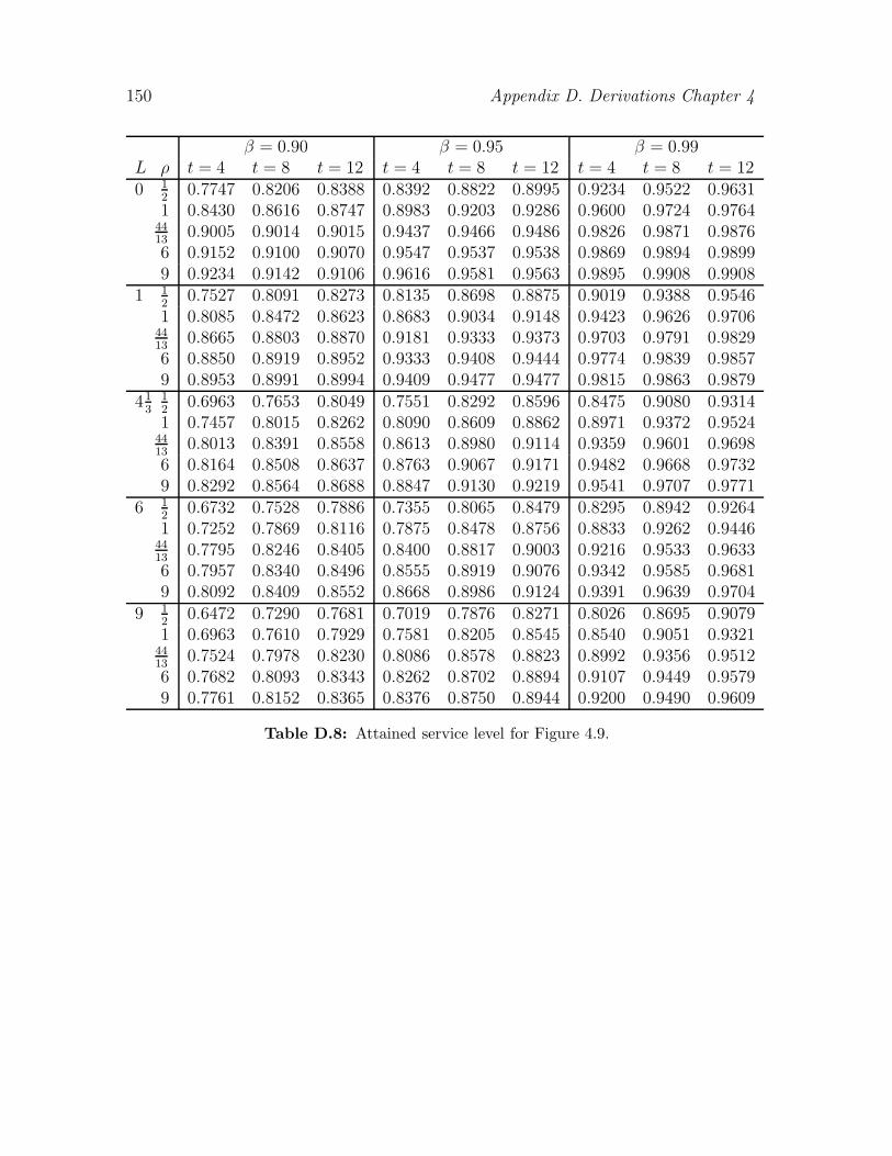
150 Appendix D. Derivations Chapter 4
β = 0.90 β = 0.95 β = 0.99L ρ t = 4 t = 8 t = 12 t = 4 t = 8 t = 12 t = 4 t = 8 t = 120 1
20.7747 0.8206 0.8388 0.8392 0.8822 0.8995 0.9234 0.9522 0.9631
1 0.8430 0.8616 0.8747 0.8983 0.9203 0.9286 0.9600 0.9724 0.97644413
0.9005 0.9014 0.9015 0.9437 0.9466 0.9486 0.9826 0.9871 0.98766 0.9152 0.9100 0.9070 0.9547 0.9537 0.9538 0.9869 0.9894 0.98999 0.9234 0.9142 0.9106 0.9616 0.9581 0.9563 0.9895 0.9908 0.9908
1 12
0.7527 0.8091 0.8273 0.8135 0.8698 0.8875 0.9019 0.9388 0.95461 0.8085 0.8472 0.8623 0.8683 0.9034 0.9148 0.9423 0.9626 0.97064413
0.8665 0.8803 0.8870 0.9181 0.9333 0.9373 0.9703 0.9791 0.98296 0.8850 0.8919 0.8952 0.9333 0.9408 0.9444 0.9774 0.9839 0.98579 0.8953 0.8991 0.8994 0.9409 0.9477 0.9477 0.9815 0.9863 0.9879
413
12
0.6963 0.7653 0.8049 0.7551 0.8292 0.8596 0.8475 0.9080 0.93141 0.7457 0.8015 0.8262 0.8090 0.8609 0.8862 0.8971 0.9372 0.95244413
0.8013 0.8391 0.8558 0.8613 0.8980 0.9114 0.9359 0.9601 0.96986 0.8164 0.8508 0.8637 0.8763 0.9067 0.9171 0.9482 0.9668 0.97329 0.8292 0.8564 0.8688 0.8847 0.9130 0.9219 0.9541 0.9707 0.9771
6 12
0.6732 0.7528 0.7886 0.7355 0.8065 0.8479 0.8295 0.8942 0.92641 0.7252 0.7869 0.8116 0.7875 0.8478 0.8756 0.8833 0.9262 0.94464413
0.7795 0.8246 0.8405 0.8400 0.8817 0.9003 0.9216 0.9533 0.96336 0.7957 0.8340 0.8496 0.8555 0.8919 0.9076 0.9342 0.9585 0.96819 0.8092 0.8409 0.8552 0.8668 0.8986 0.9124 0.9391 0.9639 0.9704
9 12
0.6472 0.7290 0.7681 0.7019 0.7876 0.8271 0.8026 0.8695 0.90791 0.6963 0.7610 0.7929 0.7581 0.8205 0.8545 0.8540 0.9051 0.93214413
0.7524 0.7978 0.8230 0.8086 0.8578 0.8823 0.8992 0.9356 0.95126 0.7682 0.8093 0.8343 0.8262 0.8702 0.8894 0.9107 0.9449 0.95799 0.7761 0.8152 0.8365 0.8376 0.8750 0.8944 0.9200 0.9490 0.9609
Table D.8: Attained service level for Figure 4.9.

D.3. Simulation results 151
β = 0.90 β = 0.95 β = 0.99L ρ t = 4 t = 8 t = 12 t = 4 t = 8 t = 12 t = 4 t = 8 t = 120 1
20.8344 0.8681 0.8789 0.8912 0.9219 0.9316 0.9564 0.9747 0.9802
1 0.8651 0.8820 0.8931 0.9175 0.9374 0.9441 0.9704 0.9811 0.98414413
0.8862 0.8959 0.8988 0.9363 0.9442 0.9481 0.9806 0.9869 0.98816 0.8887 0.8955 0.8974 0.9398 0.9455 0.9486 0.9827 0.9873 0.98889 0.8885 0.8936 0.8963 0.9420 0.9461 0.9481 0.9841 0.9875 0.9886
1 12
0.8387 0.8712 0.8789 0.8929 0.9237 0.9307 0.9569 0.9734 0.98021 0.8608 0.8869 0.8937 0.9145 0.9355 0.9413 0.9677 0.9802 0.98404413
0.8805 0.8925 0.8972 0.9311 0.9443 0.9466 0.9771 0.9847 0.98756 0.8855 0.8946 0.8981 0.9374 0.9449 0.9484 0.9807 0.9864 0.98829 0.8873 0.8956 0.8975 0.9394 0.9478 0.9484 0.9828 0.9874 0.9891
413
12
0.8283 0.8638 0.8826 0.8847 0.9191 0.9300 0.9471 0.9710 0.97661 0.8529 0.8780 0.8867 0.9045 0.9268 0.9377 0.9598 0.9774 0.98164413
0.8686 0.8881 0.8939 0.9182 0.9388 0.9429 0.9676 0.9819 0.98616 0.8716 0.8911 0.8947 0.9229 0.9396 0.9434 0.9732 0.9837 0.98609 0.8763 0.8916 0.8962 0.9249 0.9419 0.9447 0.9753 0.9849 0.9878
6 12
0.8272 0.8645 0.8775 0.8809 0.9140 0.9282 0.9459 0.9692 0.97791 0.8499 0.8770 0.8829 0.9034 0.9268 0.9363 0.9593 0.9759 0.98154413
0.8685 0.8891 0.8914 0.9169 0.9372 0.9428 0.9670 0.9824 0.98526 0.8737 0.8922 0.8953 0.9223 0.9399 0.9444 0.9713 0.9836 0.98639 0.8821 0.8949 0.8972 0.9277 0.9432 0.9464 0.9736 0.9855 0.9871
9 12
0.8231 0.8620 0.8747 0.8781 0.9118 0.9263 0.9447 0.9669 0.97471 0.8512 0.8741 0.8833 0.9022 0.9261 0.9335 0.9562 0.9751 0.98104413
0.8740 0.8890 0.8934 0.9160 0.9367 0.9431 0.9661 0.9809 0.98496 0.8828 0.8970 0.9014 0.9243 0.9438 0.9453 0.9693 0.9848 0.98729 0.8893 0.9016 0.9039 0.9323 0.9465 0.9495 0.9743 0.9861 0.9885
Table D.9: Attained service level for Figure 4.11.

152 Appendix D. Derivations Chapter 4
β = 0.90 β = 0.95 β = 0.99L ρ t = 4 t = 8 t = 12 t = 4 t = 8 t = 12 t = 4 t = 8 t = 120 1
20.8988 0.9000 0.8979 0.9488 0.9498 0.9495 0.9892 0.9895 0.9896
1 0.9004 0.8966 0.9014 0.9494 0.9507 0.9517 0.9897 0.9891 0.98894413
0.8992 0.8999 0.9009 0.9495 0.9489 0.9506 0.9891 0.9899 0.98986 0.8969 0.8979 0.8985 0.9490 0.9485 0.9501 0.9888 0.9894 0.98999 0.8944 0.8952 0.8970 0.9490 0.9482 0.9491 0.9889 0.9892 0.9895
1 12
0.9012 0.9015 0.8982 0.9494 0.9515 0.9482 0.9899 0.9899 0.99011 0.9003 0.9031 0.9030 0.9518 0.9507 0.9506 0.9905 0.9899 0.99004413
0.9001 0.8990 0.9006 0.9512 0.9510 0.9502 0.9896 0.9893 0.98986 0.9000 0.8989 0.9003 0.9518 0.9498 0.9508 0.9900 0.9897 0.98999 0.8986 0.8989 0.8991 0.9511 0.9515 0.9503 0.9902 0.9899 0.9904
413
12
0.8987 0.9004 0.9033 0.9498 0.9509 0.9496 0.9895 0.9903 0.98941 0.9004 0.8990 0.8989 0.9501 0.9482 0.9499 0.9911 0.9898 0.98974413
0.8970 0.8983 0.8993 0.9486 0.9494 0.9488 0.9891 0.9891 0.99006 0.8951 0.8986 0.8986 0.9475 0.9480 0.9479 0.9896 0.9892 0.98919 0.8961 0.8979 0.8994 0.9460 0.9488 0.9484 0.9894 0.9895 0.9902
6 12
0.8999 0.8986 0.8993 0.9483 0.9488 0.9489 0.9887 0.9898 0.99021 0.9003 0.8985 0.8960 0.9519 0.9476 0.9488 0.9909 0.9900 0.98974413
0.8998 0.9003 0.8975 0.9492 0.9492 0.9494 0.9900 0.9900 0.98976 0.8986 0.9006 0.8997 0.9490 0.9490 0.9492 0.9895 0.9898 0.98959 0.9030 0.9020 0.9009 0.9503 0.9509 0.9505 0.9895 0.9903 0.9899
9 12
0.8964 0.8991 0.8996 0.9486 0.9467 0.9494 0.9899 0.9892 0.98871 0.9048 0.8986 0.8975 0.9542 0.9499 0.9475 0.9914 0.9903 0.99044413
0.9082 0.9013 0.9000 0.9517 0.9495 0.9500 0.9912 0.9898 0.98976 0.9092 0.9067 0.9063 0.9529 0.9537 0.9508 0.9905 0.9913 0.99079 0.9118 0.9091 0.9081 0.9564 0.9547 0.9539 0.9910 0.9914 0.9914
Table D.10: All attained service levels for Table 4.17.

D.3. Simulation results 153
α = 0.90 α = 0.95 α = 0.99OUL L t = 4 t = 8 t = 12 t = 4 t = 8 t = 12 t = 4 t = 8 t = 12Using α
0 0.8172 0.8659 0.8709 0.8670 0.9146 0.9232 0.9232 0.9623 0.97041 0.7923 0.8410 0.8381 0.8377 0.8923 0.8973 0.8980 0.9456 0.95294 0.7297 0.7719 0.8106 0.7733 0.8292 0.8642 0.8357 0.8994 0.9280
Using α′
0 0.8737 0.8950 0.8917 0.9198 0.9385 0.9417 0.9629 0.9799 0.98181 0.8435 0.8723 0.8607 0.8935 0.9205 0.9188 0.9492 0.9666 0.96594 0.7796 0.8059 0.8309 0.8315 0.8637 0.8831 0.9077 0.9341 0.9499
Using kα0 0.8906 0.9044 0.8993 0.9351 0.9493 0.9488 0.9764 0.9838 0.98701 0.8817 0.8972 0.8849 0.9268 0.9409 0.9367 0.9709 0.9794 0.97644 0.8569 0.8649 0.8753 0.9033 0.9156 0.9241 0.9539 0.9691 0.9725
Table D.11: Attained service level for Figure 4.13.
β = 0.90 β = 0.95 β = 0.99OUL L t = 4 t = 8 t = 12 t = 4 t = 8 t = 12 t = 4 t = 8 t = 12Using β
0 0.8163 0.8689 0.8739 0.8640 0.9192 0.9290 0.9150 0.9634 0.97621 0.7966 0.8699 0.8545 0.8392 0.9194 0.9048 0.8874 0.9654 0.95654 0.7705 0.7950 0.8131 0.8244 0.8592 0.8684 0.8868 0.9280 0.9341
Using β ′
0 0.8700 0.8994 0.8960 0.9123 0.9444 0.9488 0.9524 0.9777 0.98591 0.8443 0.9004 0.8750 0.8841 0.9449 0.9247 0.9374 0.9803 0.96744 0.8318 0.8334 0.8330 0.8836 0.8964 0.8925 0.9353 0.9519 0.9585
Using kβ0 0.8706 0.9030 0.9063 0.9133 0.9475 0.9536 0.9551 0.9795 0.98871 0.8624 0.9184 0.8922 0.9064 0.9585 0.9384 0.9554 0.9865 0.97594 0.8931 0.8932 0.8845 0.9281 0.9402 0.9322 0.9643 0.9760 0.9811
Table D.12: Attained service level for Figure 4.14.

154 Appendix D. Derivations Chapter 4
α = 0.90 α = 0.95 α = 0.99L ρ t = 4 t = 8 t = 12 t = 4 t = 8 t = 12 t = 4 t = 8 t = 120 1
21.4562 1.1883 1.1250 1.7770 1.3169 1.2169 2.7866 1.6461 1.3977
1 1.2208 1.0926 1.0644 1.3544 1.1480 1.1013 1.7590 1.3144 1.22742 1.1110 1.0470 1.0300 1.2008 1.0755 1.0488 1.4242 1.1779 1.10914 1.0651 1.0220 1.0186 1.1144 1.0433 1.0264 1.2806 1.0930 1.06036 1.0487 1.0174 1.0112 1.0871 1.0337 1.0187 1.2152 1.0658 1.04708 1.0382 1.0114 1.0117 1.0765 1.0259 1.0144 1.1793 1.0710 1.037510 1.0356 1.0106 1.0088 1.0676 1.0236 1.0143 1.1708 1.0686 1.0317
12
12
1.6414 1.2726 1.1674 1.9821 1.3997 1.2599 3.2745 1.7831 1.49581 1.3045 1.1433 1.0901 1.4575 1.2134 1.1444 1.8399 1.3682 1.24302 1.1577 1.0690 1.0450 1.2440 1.1072 1.0673 1.4943 1.2014 1.12784 1.0932 1.0397 1.0278 1.1484 1.0664 1.0390 1.2992 1.1172 1.07796 1.0662 1.0296 1.0231 1.1122 1.0463 1.0308 1.2402 1.0951 1.05448 1.0530 1.0227 1.0151 1.0960 1.0410 1.0266 1.1956 1.0803 1.052810 1.0464 1.0217 1.0146 1.0792 1.0296 1.0222 1.1684 1.0664 1.0475
1 12
1.7432 1.3281 1.2135 2.1574 1.4774 1.3054 3.3868 1.8762 1.52541 1.3485 1.1665 1.1089 1.5134 1.2330 1.1531 1.9991 1.3972 1.27342 1.1928 1.0857 1.0616 1.2894 1.1292 1.0917 1.5150 1.2187 1.14964 1.1095 1.0521 1.0357 1.1684 1.0822 1.0496 1.3194 1.1387 1.09186 1.0844 1.0408 1.0253 1.1284 1.0523 1.0382 1.2436 1.1013 1.07088 1.0697 1.0319 1.0220 1.1083 1.0434 1.0332 1.2079 1.0867 1.055310 1.0584 1.0275 1.0187 1.0887 1.0376 1.0263 1.1752 1.0764 1.0485
3 12
2.0505 1.4391 1.2824 2.5880 1.6369 1.3853 4.4704 2.0870 1.67041 1.4893 1.2268 1.1562 1.6934 1.3166 1.2177 2.2799 1.5306 1.35022 1.2659 1.1305 1.0838 1.3567 1.1788 1.1164 1.6381 1.2960 1.19334 1.1553 1.0766 1.0569 1.2171 1.1099 1.0721 1.3659 1.1705 1.11796 1.1204 1.0585 1.0398 1.1674 1.0784 1.0525 1.2878 1.1287 1.08678 1.1000 1.0496 1.0357 1.1352 1.0645 1.0465 1.2332 1.1134 1.077110 1.0869 1.0409 1.0301 1.1187 1.0588 1.0384 1.2040 1.0996 1.0683
6 12
2.2445 1.5189 1.3463 2.9569 1.7501 1.4661 5.2085 2.3673 1.80671 1.5962 1.2822 1.1893 1.8406 1.3846 1.2594 2.4657 1.6115 1.41022 1.3238 1.1657 1.1102 1.4473 1.2242 1.1500 1.7320 1.3566 1.24004 1.1923 1.1019 1.0690 1.2687 1.1368 1.0957 1.4206 1.2118 1.14856 1.1495 1.0786 1.0541 1.1958 1.1051 1.0767 1.3255 1.1593 1.11108 1.1197 1.0640 1.0463 1.1650 1.0877 1.0619 1.2744 1.1373 1.093010 1.1057 1.0576 1.0388 1.1445 1.0768 1.0519 1.2248 1.1184 1.0820
Table D.13: Values corrections for Figure 4.5.

D.3. Simulation results 155
β = 0.90 β = 0.95 β = 0.99L ρ t = 4 t = 8 t = 12 t = 4 t = 8 t = 12 t = 4 t = 8 t = 120 1
22.1065 1.5378 1.3422 2.5853 1.6504 1.4471 3.7405 2.1279 1.6209
1 1.3631 1.1907 1.1380 1.4859 1.2372 1.1805 1.8366 1.3866 1.28552 1.0977 1.0466 1.0324 1.1594 1.0727 1.0594 1.3352 1.1692 1.10284 0.9809 0.9834 0.9928 1.0027 0.9979 0.9971 1.1269 1.0437 1.03656 0.9439 0.9683 0.9810 0.9711 0.9768 0.9833 1.0631 1.0119 1.00318 0.9323 0.9605 0.9718 0.9514 0.9676 0.9805 1.0182 0.9925 0.987510 0.9206 0.9560 0.9703 0.9393 0.9640 0.9711 1.0010 0.9857 0.9814
12
12
2.1229 1.5078 1.3441 2.6210 1.6866 1.4471 4.0146 2.0935 1.69091 1.4043 1.2038 1.1420 1.5721 1.2721 1.1925 1.9905 1.4798 1.32722 1.1579 1.0860 1.0544 1.2242 1.1058 1.0766 1.4445 1.2073 1.13554 1.0428 1.0238 1.0158 1.0776 1.0322 1.0241 1.2104 1.0867 1.06576 1.0043 0.9970 0.9977 1.0250 1.0113 1.0041 1.1154 1.0451 1.02478 0.9869 0.9854 0.9932 1.0003 0.9947 0.9950 1.0781 1.0295 1.011910 0.9737 0.9841 0.9882 0.9891 0.9871 0.9949 1.0428 1.0074 1.0076
1 12
2.1626 1.5107 1.3296 2.5951 1.6396 1.4611 4.3824 2.1214 1.69481 1.4522 1.2251 1.1523 1.6037 1.3012 1.2000 2.1387 1.4912 1.32672 1.1861 1.0956 1.0668 1.2774 1.1377 1.0911 1.4948 1.2398 1.15184 1.0730 1.0351 1.0240 1.1237 1.0593 1.0396 1.2447 1.1086 1.06226 1.0391 1.0145 1.0112 1.0694 1.0288 1.0184 1.1665 1.0629 1.03888 1.0141 1.0050 1.0037 1.0350 1.0133 1.0112 1.1065 1.0444 1.026810 1.0014 1.0005 0.9983 1.0218 1.0072 1.0038 1.0826 1.0345 1.0150
3 12
2.2784 1.5300 1.3515 2.8426 1.7342 1.4719 4.8252 2.2884 1.76631 1.5369 1.2676 1.1638 1.7518 1.3560 1.2290 2.3281 1.5601 1.36782 1.2678 1.1363 1.0889 1.3702 1.1864 1.1285 1.6694 1.2871 1.20134 1.1431 1.0700 1.0481 1.1978 1.0998 1.0673 1.3279 1.1677 1.11516 1.0971 1.0484 1.0331 1.1343 1.0695 1.0484 1.2339 1.1160 1.07648 1.0741 1.0388 1.0272 1.1034 1.0528 1.0362 1.1853 1.0921 1.059010 1.0614 1.0306 1.0214 1.0826 1.0445 1.0280 1.1531 1.0758 1.0520
6 12
2.4791 1.6024 1.3836 3.0792 1.8474 1.5171 5.5196 2.4841 1.85891 1.6163 1.2960 1.1982 1.8605 1.4093 1.2821 2.5789 1.6308 1.44322 1.3249 1.1697 1.1127 1.4489 1.2292 1.1537 1.7359 1.3598 1.23674 1.1924 1.1000 1.0687 1.2495 1.1330 1.0920 1.4007 1.1969 1.13686 1.1359 1.0727 1.0502 1.1815 1.0969 1.0697 1.2902 1.1488 1.10528 1.1102 1.0591 1.0411 1.1468 1.0807 1.0556 1.2353 1.1184 1.081310 1.0919 1.0494 1.0341 1.1231 1.0671 1.0462 1.2000 1.1031 1.0689
Table D.14: Values corrections for Figure 4.10.

Appendix E
Derivations Chapter 5
E.1 Fitting a mixed-Erlang distribution
If X is a mixed-Erlang distributed variable, its pdf (f(x)) is the mixture of the pdfs
of two Erlang distributed variables:
f(x) = p1µk11
xk1−1
(k1 − 1)!e−µ1x + p2µ
k22
xk2−1
(k2 − 1)!e−µ2x.
Hence, such a distribution has six parameters: p1, p2, k1, k2, µ1, and µ2. These
parameters are nonnegative, p1 + p2 = 1, and k1, k2 ∈ N.
Note that the expected value and variance of X are
E [X ] = p1k1µ1
+ p2k2µ2,
and
V [X ] = p1k1µ21
(1 + k1) + p2k2µ22
(1 + k2)− p21k21µ21
− p22k22µ22
− 2p1p2k1k2µ1µ2
.
The coefficient of variation of X is determined using CX =√
V [X ]/E [X ]. Since we
have five unknown demand parameters (p2 = 1 − p1), we would need the first five
moments to fit a mixed-Erlang distribution. Methods exist that use only the first two
moments, see Tijms (1994), Van der Heijden (1993), and Janssen (1998). In Chapter
5 the method described by Janssen (1998) is used to fit a mixed-Erlang distribution
158 Appendix E. Derivations Chapter 5
to the first two moments:
if CX < 1 if CX ≥ 1
k1 =
⌊1
C2X
⌋k1 = 1
k2 = k1 + 1 k2 = 1
p1 =k2C
2X −
√k2(1 + C2
X)− k22C
2X
1 + C2X
µ1 =2
E [X ]
(1 +
√C2
X − 12
C2X + 1
)
p2 = 1− p1 µ2 =4
E [X ]− µ1
µ1 =k2 − p1E [X ]
p1 =µ1 (µ2E [X ]− 1)
µ2 − µ1
µ2 = µ1 p2 = 1− p1.
(E.1)
We use ζ to denote all the parameters of the mixed-Erlang distribution, so
ζ = [p1, p2, k1, k2, µ1, µ2].
Let Dℓ denote the demand during ℓ periods. We assume that DR can be accurately
fitted to a mixed Erlang distribution with parameters ζ = [p1, p2, k1, k2, µ1, µ2] and
DL to a mixed Erlang distribution with parameters η = [q1, q2, l1, l2, λ1, λ2].
E.2 Expected backlog at start replenishment cycle
This appendix provides the derivation of the expected backlog at the start of the
replenishment cycle (E [(DL − S)+]); it is based on Janssen (1998). We assume that
the demand during lead time is mixed Erlang distributed with parameters q1, q2,
l1, l2, λ1, and λ2. Furthermore, let hl,λ(x) denote the pdf of an Erlang distributed
variable and Hl,λ(x) its cdf. We have closed form expressions for these, namely:
hl,λ(x) = λl xl−1
(l − 1)!e−λx,
Hl,λ(x) = 1− e−λxl−1∑
t=0
(λx)t
t!.
If S is assumed to be fixed and fη(x) denotes the pdf of DL, we can determine
E.2. Expected backlog at start replenishment cycle 159
the expected backlog as follows:
E[(DL − S)+
]
=
∫ ∞
S
(x− S)fη(x)dx
=
∫ ∞
S
(x− S)2∑
j=1
qjλljj
xlj−1
(lj − 1)!e−λjxdx
=
2∑
j=1
qj
∫ ∞
S
(x− S)λljj
xlj−1
(lj − 1)!e−λjxdx
=2∑
j=1
qj
(∫ ∞
S
xλljj
xlj−1
(lj − 1)!e−λjxdx− S
∫ ∞
S
λljj
xlj−1
(lj − 1)!e−λjxdx
)
=2∑
j=1
qj
(∫ ∞
S
λljj
xlj
(lj − 1)!e−λjxdx− S(1−Hlj ,λj
(S))
)
=
2∑
j=1
qj
(∫ ∞
S
λlj+1j
xlj
lj !e−λjx
lj!
λj(lj − 1)!dx− S(1−Hlj ,λj
(S))
)
=
2∑
j=1
qj
(ljλj
∫ ∞
S
λlj+1j
xlj
lj !e−λjxdx− S(1−Hlj ,λj
(S))
)
=2∑
j=1
qj
(ljλj
(1−Hlj+1,λj(S))− S(1−Hlj ,λj
(S))
)
=
2∑
j=1
qj
ljλj
lj∑
t=0
(λjS)t
t!e−λjS − S
lj−1∑
t=0
(λjS)t
t!e−λjS
.
Note that it is a closed form expression containing sums with a finite number of
terms.
If S is assumed to be random, it can be fitted to a mixed Erlang distribution with
parameters w1, w2, m1, m2, ρ1, and ρ2; the pdf that belongs to this mixed Erlang
distribution is denoted by fξ(x). The derivation is as follows:
E[(DL − S)+
]
=
∫ ∞
0
∫ ∞
z
(x− z)fη(x)dxfξ(z)dz
=
∫ ∞
0
∫ ∞
z
(x− z)fη(x)fξ(z)dxdz

160 Appendix E. Derivations Chapter 5
=
∫ ∞
0
∫ ∞
z
(x− z)
2∑
j=1
qjλljj
xlj−1
(lj − 1)!e−λjx
2∑
i=1
wiρmi
i
zmi−1
(mi − 1)!e−ρizdxdz
=2∑
j=1
2∑
i=1
qjwi
∫ ∞
0
∫ ∞
z
(x− z)λljj
xlj−1
(lj − 1)!e−λjxρmi
i
zmi−1
(mi − 1)!e−ρizdxdz
=2∑
j=1
2∑
i=1
qjwi
∫ ∞
0
ρmi
i
zmi−1
(mi − 1)!e−ρiz
∫ ∞
z
(x− z)λljj
xlj−1
(lj − 1)!e−λjxdxdz
=
2∑
j=1
2∑
i=1
qjwi
(∫ ∞
0
ρmi
i
zmi−1
(mi − 1)!e−ρiz
∫ ∞
z
xλljj
xlj−1
(lj − 1)!e−λjxdxdz
−∫ ∞
0
ρmi
i
zmi−1
(mi − 1)!e−ρiz
∫ ∞
z
zλljj
xlj−1
(lj − 1)!e−λjxdxdz
)
=
2∑
j=1
2∑
i=1
qjwi
(∫ ∞
0
ρmi
i
zmi−1
(mi − 1)!e−ρiz
lj !
λj(lj − 1)!
∫ ∞
z
λlj+1j
xlj
lj !e−λjxdxdz
−∫ ∞
0
ρmi
i
zmi−1
(mi − 1)!e−ρizz
∫ ∞
z
λljj
xlj−1
(lj − 1)!e−λjxdxdz
)
=2∑
j=1
2∑
i=1
qjwi
(∫ ∞
0
ρmi
i
zmi−1
(mi − 1)!e−ρiz
ljλj
(1−Hlj+1,λj(z))dz
−∫ ∞
0
ρmi
i
zmi−1
(mi − 1)!e−ρizz(1 −Hlj ,λj
(z))dz
)
=2∑
j=1
2∑
i=1
qjwi
∫ ∞
0
ρmi
i
zmi−1
(mi − 1)!e−ρiz
ljλj
lj∑
t=0
(λjz)t
t!e−λjzdz
−∫ ∞
0
ρmi
i
zmi−1
(mi − 1)!e−ρizz
lj−1∑
t=0
(λjz)t
t!e−λjzdz
=
2∑
j=1
2∑
i=1
qjwi
lj∑
t=0
ljρmi
i λtj
λj(mi − 1)!t!
∫ ∞
0
zmi−1e−ρizzte−λjzdz
−lj−1∑
t=0
ρmi
i λtj
(mi − 1)!t!
∫ ∞
0
zmi−1e−ρizzzte−λjzdz
=
2∑
j=1
2∑
i=1
qjwi
lj∑
t=0
ljρmi
i λt−1j
(mi − 1)!t!
∫ ∞
0
zmi+t−1e−(λj+ρi)zdz
−lj−1∑
t=0
ρmi
i λtj
(mi − 1)!t!
∫ ∞
0
zmi+te−(λj+ρi)zdz

E.3. Distribution of demand during lead time and review period 161
=
2∑
j=1
2∑
i=1
qjwi
lj∑
t=0
ljρmi
i λt−1j
(mi − 1)!t!
(mi + t− 1)!
(λj + ρi)mi+t
∫ ∞
0
(λj + ρi)mi+t zmi+t−1
(mi + t− 1)!e−(λj+ρi)zdz
−lj−1∑
t=0
ρmi
i λtj
(mi − 1)!t!
(mi + t)!
(λj + ρi)mi+t+1
∫ ∞
0
(λj + ρi)mi+t+1 zmi+t
(mi + t)!e−(λj+ρi)zdz
=2∑
j=1
2∑
i=1
qjwi
lj∑
t=0
ljρmi
i λt−1j
(mi − 1)!t!
(mi + t− 1)!
(λj + ρi)mi+t
∫ ∞
0
hmi+t,λj+ρi(z)dz
−lj−1∑
t=0
ρmi
i λtj
(mi − 1)!t!
(mi + t)!
(λj + ρi)mi+t+1
∫ ∞
0
hmi+t+1,λj+ρi(z)dz
=
2∑
j=1
2∑
i=1
qjwi
lj∑
t=0
ljρmi
i λt−1j (mi + t− 1)!
(mi − 1)!t!(λj + ρi)mi+t
−lj−1∑
t=0
ρmi
i λtj(mi + t)!
(mi − 1)!t!(λj + ρi)mi+t+1
.
Note that again we have a closed form expression containing sums with a finite
number of terms.
E.3 Distribution of demand during lead time and
review period
As stated in Section 5.2 the mixed Erlang distribution is a special case of the phase
type distribution. Since the phase type distribution is not a well-known distribution,
this distribution is introduced in short.
A phase type distributed variable X consist of the sum of a (possibly random)
number of exponentially distributed variables, possibly with different scale param-
eters. The phase type distribution can easily be linked to a Markov process; X
measures the time until absorption in the corresponding Markov process. For a thor-
ough introduction in phase type distributions see Neuts (1981) and Latouche and
Ramaswami (1999).

162 Appendix E. Derivations Chapter 5
1
k1+1
2
k1+2
k1. . .
. . . k1+k2
0
p1
p2
µ1
µ2
µ1
µ2
µ1
µ2
µ1
µ2
Figure E.1: The Markov process belonging to a mixed Erlang distribution.
Let us consider the mixed Erlang distribution. The corresponding Markov pro-
cess is depicted in Figure E.1. The parameters p1 and p2 are the probabilities of
drawing from either the first or the second Erlang distribution. The states 1, . . . , k1
belong to that first distribution and the time it takes to get from state 1 to state
0 is the sum of k1 exponentially distributed transition times with rate µ1, so it is
indeed Erlang distributed with shape parameter k1 and scale parameter 1/µ1. The
states k1 + 1, . . . , k1 + k2 belong to the second Erlang distribution of the mixture of
two Erlangs; the time it takes to get from state k1+1 to 0 is the sum of k2 exponen-
tially distributed transition times with rate µ2, so it is Erlang distributed with shape
parameter k2 and scale parameter 1/µ2.
This Markov process is characterized by a (k1 + k2) × (k1 + k2) matrix T and a
(k1 + k2)× 1 vector τ , where:
T =
−µ1 µ1 0 . . . 0 0 0 0 0 . . . 0 00 −µ1 µ1 . . . 0 0 0 0 0 . . . 0 0...
......
. . ....
......
......
. . ....
...0 0 0 . . . −µ1 µ1 0 0 0 . . . 0 00 0 0 . . . 0 −µ1 0 0 0 . . . 0 00 0 0 . . . 0 0 −µ2 µ2 0 . . . 0 00 0 0 . . . 0 0 0 −µ2 µ2 . . . 0 0...
......
. . ....
......
......
. . ....
...0 0 0 . . . 0 0 0 0 0 . . . −µ2 µ2
0 0 0 . . . 0 0 0 0 0 . . . 0 −µ2
k1
k2
︸ ︷︷ ︸ ︸ ︷︷ ︸k1 k2
(E.2)

E.3. Distribution of demand during lead time and review period 163
and
τ =[p1 0 . . . 0 p2 0 . . . 0
].
︸ ︷︷ ︸ ︸ ︷︷ ︸k1 k2
(E.3)
The element Tij in (E.2) is the transition rate from state i to state j and the element
τ j in (E.3) denotes the probability to start in state j. According to Theorem 2.4.1 in
Latouche and Ramaswami (1999) the density and distribution functions of the phase
type distribution, characterized by T and τ , are
fT,τ (x) = τ exp(Tx)t,
FT,τ (x) = 1− τ exp(Tx)1,
where
1 =
11...1
,
t = −T1,
and
exp(A) =
∞∑
i=0
1
i!Ai.
Since both DR and DL are mixed Erlang distributed, they are phase type dis-
tributed with parameters TR and τR and with TL and τL. According to Theorem
2.6.1 in Latouche and Ramaswami (1999) the sum of DR and DL, DR+L, is again
phase type distributed, with parameters
TR+L =
[TR tR · τL
0 TL
],
τR+L =[τR τ 0RτL
],
where
tR = −TR1,
τ 0R = 1− τR1.
Note that τR1 = 1, since p1 + p2 = 1, hence τ 0R = 0.

164 Appendix E. Derivations Chapter 5
E.4 Expected backlog at end replenishment cycle
If S is assumed to be fixed, the expected backlog at the end of the replenishment
cycle is
E[(DR+L − S)+
]=
∫ ∞
S
(x− S)fTR+L,τR+L(x)dx,
where fTR+L,τR+Ldenotes the pdf of a phase type distribution. We can rewrite this a
little, so that we obtain
E[(DR+L − S)+
]=
∫ ∞
S
xfTR+L,τR+L(x)dx−
∫ ∞
S
SfTR+L,τR+L(x)dx
=
∫ ∞
S
xfTR+L,τR+L(x)dx− S
∫ ∞
S
fTR+L,τR+L(x)dx
=
∫ ∞
S
xfTR+L,τR+L(x)dx− S
(1− FTR+L,τR+L
(S)).
If S is random, we need to condition on the value of S and we obtain
E[(DR+L − S)+
]=
∫ ∞
0
∫ ∞
s
(x− s)fTR+L,τR+L(x)dxfξ(s)ds,
with fξ the pdf of a mixed Erlang distribution with parameters ξ. Rewriting this
expression leads to
E[(DR+L − S)+
]=
∫ ∞
0
(∫ ∞
s
xfTR+L,τR+L(x)dx− s
(1− FTR+L,τR+L
(s)))
fξ(s)ds
=
∫ ∞
0
(∫ ∞
s
xfTR+L,τR+L(x)dx
)fξ(s)ds−
∫ ∞
0
sfξ(s)ds
+
∫ ∞
0
sFTR+L,τR+L(s)fξ(s)ds
=
∫ ∞
0
(∫ ∞
s
xfTR+L,τR+L(x)dx
)fξ(s)ds−
(w1
m1
ρ1+ w2
m2
ρ2
)
+
∫ ∞
0
sFTR+L,τR+L(s)fξ(s)ds.
Note that both the cdf and pdf of a phase type distributed variable depend on
exp(Tx), which is an infinite sum. Latouche and Ramaswami (1999) provide an
algorithm to determine the value of FT,τ (x). We first need to define two variables,
depending on the n× n-matrix T :
c = max{−Tii}, i ∈ {1, . . . , n},P = 1
cT + I,

E.4. Expected backlog at end replenishment cycle 165
where I is the identity matrix. Note that c is the maximum of the negative of the
diagonal of T and thus the diagonal elements of P are all less than or equal to one.
The value of FT,τ (x) can now be determined numerically by the following algorithm
(ǫ provides the precision):
M := τ (I − P )−1;a0 := τ1;k := 0;v := P1;repeatk := k + 1;ak := τv;v := Pv;
until |∑k
i=0 ai −M | < ǫ;K1 := k;for any x of interest dop := e−cx
Y := pa0;for k := 1 to K1 dop := p cx
k;
Y := Y + pak;od
odFT,τ (x) = 1− Y.
A similar algorithm can be provided for fT,τ (x).


Bibliography
Artto, K. A. and E. Pylkkanen (1999). An effective procedure for the distribution
of magazines. International Transactions in Operational Research, 289–310.
Ashayeri, J., R. J. M. Heuts, H. G. L. Lansdaal, and L. W. G. Strijbosch (2006).
Cyclic production-inventory planning and control in the pre-Deco industry: a
case study. International Journal of Production Economics , 715–725.
Azoury, K. S. (1985). Bayes solution to dynamic inventory models under unknown
demand distribution. Management Science, 1150–1160.
Azoury, K. S. and B. L. Miller (1984). A comparison of the optimal ordering levels
of Bayesian and non-Bayesian inventory models. Management Science, 993–
1003.
Bertsimas, D. and A. Thiele (2006). A robust optimization approach to inventory
theory. Operations Research, 150–168.
Bookbinder, J. H. and A. E. Lordahl (1989). Estimation of inventory reorder level
using the bootstrap statistical procedure. IIE Transactions , 302–312.
Bulinskaya, E. V. (1990). Inventory control in case of unknown demand distribu-
tion. Engineering Costs and Production Economics , 301–306.
Burgin, T. A. (1975). The gamma distribution and inventory control. Operational
Research Quarterly , 507–525.
Evans, M., N. Hastings, and B. Peacock (2000). Statistical distributions (3 ed.).
Wiley series in probability and statistics. New York: John Wiley & Sons, Inc.
Fricker, R. D. and C. A. Goodhart (2000). Applying a bootstrap approach for
setting reorder points in military supply systems. Naval Research Logistics ,
459–478.

168 Bibliography
Hayes, R. H. (1969). Statistical estimation problems in inventory control. Manage-
ment Science, 686–701.
Heijden, M. C. van der (1993). Performance analysis for reliability and inventory
models. Ph. D. thesis, Free University of Amsterdam.
Janssen, E., L. W. G. Strijbosch, and R. C. M. Brekelmans (2007). How to deter-
mine the order-up-to level when demand is gamma distributed with unknown
parameters. Center discussion paper, Tilburg University.
Janssen, E., L. W. G. Strijbosch, and R. C. M. Brekelmans (2009). Assessing
the effects of using demand parameters estimates in inventory control and im-
proving the performance using a correction function. International Journal of
Production Economics , 34–42.
Janssen, F. B. S. L. P. (1998). Inventory management systems control and infor-
mation issues. Ph. D. thesis, Tilburg University.
Janssen, F. B. S. L. P., R. J. M. Heuts, and A. G. de Kok (1998). On the (R, s,Q)
inventory model when demand is modelled as a compound Bernoulli process.
European Journal of Operational Research, 423–436.
Kaplan, R. S. (1970). A dynamic inventory model with stochastic lead times. Man-
agement Science, 491–507.
Karmarkar, U. S. (1994). A robust forecasting technique for inventory and leadtime
management. Journal of Operations Management , 45–54.
Kottas, J. F. and H.-S. Lau (1980). The use of versatile distribution families in
some stochastic inventory calculations. The Journal of the Operational Research
Society , 393–403.
Larson, C. E., L. J. Olson, and S. Sharma (2001). Optimal inventory policies when
the demand distribution is not known. Journal of Economic Theory , 281–300.
Latouche, G. and V. Ramaswami (1999). Introduction to matrix analytic methods
in stochastic modeling. ASA-SIAM series on statistics and applied probability.
Philadelphia, USA: ASA SIAM.
Lau, H.-S. and A. H.-L. Lau (2003). Nonrobustness of the normal approximation
of lead-time demand in a (Q,R) system. Naval Research Logistics , 149–166.
Liyanage, L. H. and J. F. Shanthikumar (2005). A practical inventory policy using
operational statistics. Operations Research Letters , 341–348.

Bibliography 169
Lordahl, A. E. and J. H. Bookbinder (1994). Order-statistic calculation, costs and
service in an (s,Q) inventory system. Naval Research Logistics , 81–97.
Lu, X., J.-S. Song, and A. Regan (2006). Inventory planning with forecast updates:
approximate solutions and cost error bounds. Operations Research, 1079–1097.
Mittelhammer, R. C. (1996). Mathematical statistics for economics and business.
New York: Springer-Verlag.
Neuts, M. F. (1981). Matrix-geometric solutions in stochastic models. Johns Hop-
kins series in the mathematical sciences. Baltimore, USA: The Johns Hopkins
University Press.
Sani, B. and B. G. Kingsman (1997). Selecting the best periodic inventory con-
trol and demand forecasting methods for low demand items. Journal of the
Operational Research Society , 700–713.
Scarf, H. (1958). A min-max solution of an inventory problem. In K. J. Arrow,
S. Karlin, and H. E. Scarf (Eds.), Studies in the mathematical theory of inven-
tory and production, pp. 201–209. Stanford, CA: Stanford University Press.
Segerstedt, A. (1994). Inventory control with variation in lead times, especially
when demand is intermittent. International Journal of Production Economics ,
365–372.
Silver, E. A., D. F. Pyke, and R. Peterson (1998). Inventory management and
production planning and scheduling (Third ed.). New York: John Wiley &
Sons.
Silver, E. A. and M. R. Rahnama (1986). The cost effects of statistical sampling
in selecting the reorder point in a common inventory model. Journal of the
Operational Research Society , 705–713.
Silver, E. A. and M. R. Rahnama (1987). Biased selection of the inventory reorder
point when demand parameters are statistically estimated. Engineering Costs
and Production Economics , 283–292.
Silver, E. A. and D. J. Robb (2008). Some insights regarding the optimal reorder
period in periodic review inventory systems. International Journal of Produc-
tion Economics , 354–366.
Snyder, R. D., A. B. Koehler, and J. K. Ord (2002). Forecasting for inventory

170 Bibliography
control with exponential smoothing. International Journal of Forecasting , 5–
18.
Strijbosch, L. W. G. and R. M. J. Heuts (1992). Modelling (s,Q) inventory systems:
parametric versus non-parametric approximations for the lead time demand
distribution. European Journal of Operational Research, 86–101.
Strijbosch, L. W. G., R. M. J. Heuts, and E. H. M. van der Schoot (2000). A
combined forecast–inventory control procedure for spare parts. Journal of the
Operational Research Society , 1184–1192.
Strijbosch, L. W. G. and J. J. A. Moors (1999). Simple expressions for safety factors
in inventory control. Center discussion paper, Tilburg University.
Strijbosch, L. W. G. and J. J. A. Moors (2005). The impact of unknown demand
parameters on (R, S)-inventory control performance. European Journal of Op-
erational Research, 805–815.
Strijbosch, L. W. G. and J. J. A. Moors (2006). Modified normal demand distri-
butions in (R, S)-inventory control. European Journal of Operational Research,
201–212.
Strijbosch, L. W. G., J. J. A. Moors, and A. G. de Kok (1997). On the interaction
between forecasting and inventory control. Few research memorandum, Tilburg
University.
Strijbosch, L. W. G., A. A. Syntetos, J. E. Boylan, and E. Janssen (2010). On the
interaction between forecasting and stock control: the case of non-stationary
demand. Accepted for publication in: International Journal of Production Eco-
nomics .
Syntetos, A. A. and J. E. Boylan (2006). On the stock control performance of in-
termittent demand estimators. International Journal of Production Economics ,
36–47.
Thomas, D. J. (2005). Measuring item fill-rate performance in a finite horizon.
Manufacturing & Service Operations Management , 74–80.
Tijms, H. C. (1994). Stochastic models: an algorithmic approach. Chichester: John
Wiley & Sons.
Tyworth, J. E. and L. O’Neill (1997). Robustness of the normal spproximation of
lead-time demand in a distribution setting. Naval Research Logistics , 165–186.

Bibliography 171
Watson, R. B. (1987). The effects of demand-forecast fluctuations on customer ser-
vice and inventory cost when demand is lumpy. Journal of Operational Research
Society , 75–82.
Yano, C. A. and H. L. Lee (1995). Lot sizing with random yields: a review. Oper-
ations Research, 311–334.
Yeh, Q.-J. (1997). A practical implementation of gamma distribution to the re-
ordering decision of an inventory control problem. Production and Inventory
Management Journal , 51–57.
Zeng, A. Z. and J. C. Hayya (1999). The performance of two popular service mea-
sures on management effectiveness in inventory control. International Journal
of Production Economics , 147–158.
Zipkin, P. H. (2000). Foundations of inventory management. Boston: McGraw-Hill
Higher Education.


Nederlandse samenvatting
In het vakgebied voorraadbeheer gaat het erom om op een verstandige manier te
kiezen wat we wanneer bestellen en hoeveel we dan bestellen. Om deze keuze te
maken, wordt een aantal aannames gedaan omtrent het vraagproces, bijvoorbeeld
over de kansverdeling van de vraag, de verwachte vraag en de spreiding van de vraag.
Daarnaast wordt ook vaak a priori een voorraadbeleid vastgesteld. In dit proef-
schrift wordt uitgegaan van een periodieke controle van het voorraadniveau, waarna
de voorraad wordt aangevuld tot een bepaald aanvulniveau. Er wordt dan bijvoor-
beeld iedere dag, iedere week of iedere maand gecontroleerd hoe hoog de voorraad
is en dan wordt een bestelling gedaan bij een toeleverancier die zodanig groot is
dat het voorraadniveau weer op het aanvulniveau ligt. Deze bestelling wordt na een
bepaalde levertijd geleverd. De grootte van de bestelling kan dus varieren, maar de
tijd tussen bestellingen is altijd gelijk, namelijk de tijd tussen de periodieke controles
(mits er vraag naar het product is geweest tussen twee periodieke controles). In
het kort wordt dit beleid het (R, S) beleid genoemd, waarbij R de tijd tussen twee
voorraadcontroles is en S het aanvulniveau; de levertijd wordt genoteerd door L. De
waarde bij R wordt vaak van tevoren vastgesteld, bijvoorbeeld door afspraken met de
toeleverancier; de waarde van S moet zodanig gekozen worden dat er genoeg voorraad
is om aan de vraag van klanten te voldoen, maar aan de andere kant niet zo groot
zijn dat er bergen voorraad in het magazijn liggen, want dat kost geld. Geld dat
geınvesteerd is in voorraden kan immers niet voor bijvoorbeeld productontwikkeling
of een reclamecampagne gebruikt worden. De waarde van L hangt af van de toele-
verancier en de afspraken die daarmee gemaakt zijn. Soms kan worden gesteld dat
de levertijd gelijk is aan nul. Niet omdat de levering dan direct op de stoep staat,
maar omdat een bestelling die na sluitingstijd gedaan wordt, de volgende dag voor
opening aangeleverd zal zijn.
We willen het aanvulniveau dus zodanig kiezen dat de winst maximaal is (of dat
de kosten minimaal zijn). Daarvoor moeten we weten wat het kost als een product

174 Nederlandse samenvatting
niet in voorraad is wanneer een klant daarom vraagt. Maar wat doet een klant als
het product waar hij om vraagt niet op voorraad is? Gaat hij dan het product ergens
anders kopen en blijft hij dat dan ook doen? En de overige producten waarvoor de
klant kwam, wil hij die wel kopen of doet hij dat dan ook bij een ander bedrijf? Is de
klant bereid om te wachten totdat het product weer op voorraad is? Zo niet, kunnen
we een spoedbestelling plaatsen waardoor we het product sneller kunnen leveren? En
wat kost zo’n spoedbestelling dan? Dit soort overwegingen maakt het erg moeilijk
om de precieze kosten van een nee-verkoop in te kunnen schatten.
Een andere manier om een goed voorraadniveau te kiezen is door de voorraad zo
laag mogelijk te houden, maar wel hoog genoeg om aan een bepaald serviceniveau te
voldoen. In dit proefschrift worden twee definities van service gebruikt. Ten eerste
is dat de zogenoemde P1-service: deze meet de fractie aanvulcycli waarin we aan
alle vraag kunnen voldoen. Een aanvulcyclus is de tijd tussen twee opeenvolgende
leveringen. De tweede servicemaat is de zogenoemde P2-service: deze meet de fractie
van de vraag waaraan we direct kunnnen voldoen. Men kiest een bepaalde service,
zoals “in 90% van de aanvulcycli moet aan alle vraag worden voldaan” (α = 0.90) of
”95% van de vraag moet direct geleverd kunnen worden” (β = 0.95), en vervolgens
wordt S zodanig gekozen dat de gewenste service precies gehaald wordt.
In het eerste deel van dit proefschrift wordt gekeken naar nieuwe vraagverdelin-
gen, namelijk twee modified verschoven gammaverdelingen. Deze verdelingen wor-
den geconstrueerd door te beginnen met een verschoven gammaverdeling, waar-
bij negatieve realisaties mogelijk zijn; de cumulatieve verdelingsfunctie (cdf) van
deze verdeling wordt genoteerd door F en de kansdichtheidsfunctie (pdf) door f .
Een negatieve vraag is natuurlijk erg vreemd en we veranderen de verschoven gam-
maverdeling zodanig dat de negatieve realisaties verdwijnen. Je kunt dat doen door
iedere negatieve realisatie de waarde nul te geven. Dat betekent dan dat er periodes
zijn zonder vraag. De verdeling, genoteerd door F+ (cdf) en f+ (pdf), heeft een
puntmassa op nul, waarvan de waarde dus gelijk is aan de kans op nul-vraag (geno-
teerd door F (0)), en is, voor x > 0 gelijk aan een verschoven gammaverdeling. Een
tweede manier om de negatieve realisaties onmogelijk te maken is door ze simpelweg te
negeren. In de verdeling die dan ontstaat, genoteerd door F ∗ (cdf) en f ∗ (pdf), wordt
de kans op een negatieve realisatie in de verschoven gammaverdeling ‘uitgesmeerd’
over alle positieve realisaties. Zie ook de figuur bovenaan de volgende pagina voor een
grafische weergave van beide kansdichtheidsfuncties. Deze nieuwe verdelingen zorgen
ervoor dat vraagpatronen die min of meer verdeeld lijken te zijn volgens een gamma

Nederlandse samenvatting 175
x →0−∆
f+
f
F (0)
x →0−∆
f ∗
f
(a): puntmassa op x = 0. (b): afgekapt op x = 0.
Figuur: Kansdichtheidsfuncties van de modified verschoven gammaverdelingen.
verdeling op een meer flexibele manier geschat kunnen worden, aangezien deze nieuwe
verdelingen een uitbreiding vormen op de gammaverdeling; de reguliere gammaver-
deling is een speciaal geval van beide modified verschoven gammaverdelingen.
Als de vraag daadwerkelijk een van de twee modified verschoven gammaverdelin-
gen volgt, is het mogelijk om het aanvulniveau te bepalen waarbij de P1- of P2-service
gehaald wordt, als gebruik gemaakt wordt van een (R, S)-voorraadbeleid. Dit wordt
uitgewerkt in paragraaf 2.4. Aangezien deze modified verschoven gammaverdelingen
hier, voor zover bekend, voor het eerst afgeleid zijn, kan het goed zijn dat de ver-
keerde vraagverdeling gekozen wordt. Een reguliere of verschoven gammaverdeling
ligt dan voor de hand, omdat de vraag toch min of meer gamma verdeeld lijkt. De
verdelingsparameters van de reguliere gammaverdeling kunnen worden geschat met
behulp van het eerste en tweede moment van de vraag; voor de verschoven gammaver-
deling is ook het derde moment nodig. Als de reguliere of verschoven gammaverdeling
ten onrechte wordt gebruikt om de vraag te modelleren, omdat de vraag verdeeld is
volgens een modified verschoven gamma verdeling, zien we dat de behaalde service
tussen ongeveer drie procentpunten onder de gewenste service tot drie procentpunten
boven de gewenste service ligt. Dit verschil is niet heel groot, maar een behaalde ser-
vice die drie procentpunten lager ligt dan de gewenste service kan toch een heleboel
klanten, en dus omzet, kosten. Overigens is een hogere dan gewenste service ook niet
zomaar goed; het impliceert immers dat er meer voorraad aangehouden wordt dan
nodig is om de gewenste service te halen en dus dat er teveel geld geınvesteerd wordt
in voorraden.

176 Nederlandse samenvatting
Een belangrijk probleem binnen het vakgebied voorraadbeheer is dat de (verde-
ling van de) vraag onbekend is. Er zijn enkel wat historische observaties van de vraag
en aan de hand daarvan zullen we belangrijke vraaggegevens moeten schatten. Een
veelgebruikte methode is het aannemen van een bepaalde familie van verdelingen, bij-
voorbeeld de normale of de gamma verdeling, en vervolgens de verdelingsparameters
schatten aan de hand van de historische observaties. Merk op dat de schatters van
de verdelingsparameters stochasten zijn en dat het aanvulniveau een functie is van
de verdelingsparameters. Hierdoor is het aanvulniveau niet langer een determinis-
tische parameter van het voorraadbeleid, maar een stochast en hierdoor wordt extra
onzekerheid in het voorraadbeheer geıntroduceerd. De vraag is nu welke invloed deze
extra onzekerheid heeft op de behaalde service. Intuıtief geldt dat meer onzekerheid
aanleiding geeft tot het aanhouden van meer voorraad om deze onzekerheid op te
kunnen vangen. Als er geen rekening wordt gehouden met de extra onzekerheid zal
de behaalde service dus onder het gewenste niveau komen te liggen. In deel twee van
dit proefschrift wordt analytisch (voor zover mogelijk) en met behulp van simulatie
aangetoond dat dit inderdaad het geval is in het geval van normaal verdeelde, gamma
verdeelde en mixed Erlang verdeelde vraag.
In hoofdstuk 3 wordt de normale verdeling besproken. Een belangrijke aanname
is dat de vraag ook daadwerkelijk normaal verdeeld is, maar dat de verdelingspa-
rameters onbekend zijn. Onder stricte aannames kunnen we analytisch aantonen
dat de gewenste service niet gehaald wordt. In eerste instantie wordt aangenomen
dat alleen de verwachte vraag (µ) onbekend is en geschat wordt met behulp van
het steekproefgemiddelde. Zelfs in dit geval kunnen we aantonen dat zowel voor P1
als P2 de gewenste service niet gehaald wordt mits de gewenste service niet te laag
is. Dit geldt echter voor alle gangbare gewenste serviceniveau’s, dus dit levert geen
beperkingen op in de praktijk. De behaalde service ligt lager als er minder historische
waarnemingen zijn en als er meer onzekerheid in de vraag is; in beide gevallen zal de
geschatte vraag immers meer onzekerheid bevatten. Ook het gewenste serviceniveau
is van invloed, al is die invloed minder duidelijk. Men zal hiervoor naar het relatieve
verschil tussen de gewenste en behaalde service moeten kijken; dan geldt dat hoe
hoger de gewenste service, des te groter dit relatieve verschil is.
We vinden dankzij de theoretische afleiding ook een correctie: als we de stan-
daarddeviatie in de functie van het aanvulniveau vervangen door de wortel van de
voorspelfout, wordt de gewenste service weer gehaald.
Vervolgens wordt ook de spreiding van de vraag (σ2) onbekend verondersteld;

Nederlandse samenvatting 177
deze wordt geschat met behulp van de steekproefvariantie. We kunnen aantonen
dat het verwachte aanvulniveau lager is dan het aanvulniveau als alleen µ onbekend
is. Hierbij gebruiken we de analytisch gevonden correctie en veronderstellen we nog
wel dat de variatiecoefficient (ν = σ/µ) bekend is. Een lager verwacht aanvulniveau
betekent nog niet automatisch dat de gewenste service niet gehaald wordt, al is dat
wel zeer waarschijnlijk, en als we simulaties uitvoeren om dit te controleren, blijkt de
behaalde service behoorlijk onder het gewenste niveau te liggen.
Tenslotte nemen we ook aan dat de variatiecoefficient onbekend is; op dit moment
kunnen we geen analytische resultaten meer afleiden en zijn we aangewezen op simu-
latie. We gebruiken nog steeds de wortel van de geschatte voorspelfout in plaats van
de (steekproek)standaarddeviatie. Na uitvoerige simulaties blijkt dat de behaalde
service opnieuw lager uitvalt; de gemiddelde behaalde service ligt 2.03 procentpunt
onder het gewenste niveau, maar er zijn uitschieters tot bijna 12 procentpunten.
Alleen het bepalen van de mate waarin de service niet gehaald is, is niet voldoende.
Met behulp van simulatie en een nieuwe regressietechniek (geneste lineaire regressie
genaamd) is een additieve correctiefunctie gevonden. Deze functie hangt af van het
aantal historische waarnemingen, het gewenste serviceniveau en de onzekerheid in de
vraag, gemeten aan de hand van de variatiecoefficient van de vraag. Door deze cor-
rectiefunctie toe te passen met de werkelijke waarde van de variatiecoefficient van de
vraag, wordt het gewenste serviceniveau gehaald. Echter, in werkelijkheid kennen we
deze waarde niet. Ook als we deze weer vervangen door de geschatte variatiecoefficient
ligt de behaalde service wel erg dicht bij de gewenste service, namelijk binnen een
procentpunt (zie figuur 3.9).
Hoofdstuk 4 behandelt gamma verdeelde vraag, waarvan de verdelingsparameters
onbekend zijn. Qua opzet lijkt dit hoofdstuk op hoofdstuk 3. Eerst wordt enkel de
schaalparameter (θ) onbekend verondersteld. Deze wordt geschat met behulp van de
bekende waarde van de vormparameter (ρ) en het steekproefgemiddelde. Het is aan
te tonen dat deze schatter ook gamma verdeeld is en onder zeer stricte voorwaarden
(ρ = 1 en L = 0) kunnen we dan laten zien dat de gewenste service niet gehaald
wordt; zowel onder P1-service als onder P2-service. Als we deze voorwaarden wat
verzachten, we staan een positieve levertijd toe en ρ is discreet, dan kunnen we, in
geval van P1-service, numeriek laten zien dat de behaalde service onder de gewenste
service ligt voor gebruikelijke waarden van het gewenste serviceniveau. Indien we
ook ρ volledig vrij laten, zijn er geen analytische resultaten meer mogelijk en in geval
van de P2-service zijn er uberhaupt geen analytische resultaten meer mogelijk als we

178 Nederlandse samenvatting
ρ = 1 en L = 0 loslaten. In dit geval gebruiken we simulatie om te laten zien dat de
behaalde service onder het gewenste niveau ligt. Verder zien we ook dat dit verschil
groter is als ρ kleiner is, wat betekent dat de variatie in de vraag groter is. Het
verschil is groter als het aantal historische waarnemingen kleiner is, wat betekent dat
de variatie in de schatter van θ groter is. Het verschil is ook groter als de levertijd
langer is, wat betekent dat we de vraag over een langere periode moeten voorspellen
en dat zorgt weer voor meer onzekerheid. Tenslotte is het relatieve verschil groter als
de gewenste service groter is en dat is ook weer niet geheel onlogisch, aangezien een
hogere service moeilijker te behalen is.
Als ook de vormparameter onbekend wordt verondersteld, kunnen we enkel simu-
latie gebruiken om te laten zien dat de gewenste service opnieuw niet gehaald wordt
als we schatters gebruiken in plaats van de werkelijke, maar onbekende, waarde van
de verdelingparameters. Het verschil tussen de behaalde en gewenste service is boven-
dien groter dan wanneer enkel de schaalparameter onbekend is, dus we zien opnieuw
dat meer onzekerheid een lagere behaalde service impliceert. Het gemiddelde ver-
schil tussen de behaalde en gewenste service is 8.11 (P1-service) en 8.20 (P2-service)
procentpunten, met uitschieters naar bijna 30 procentpunten.
Onder de zeer stricte voorwaarden dat ρ = 1 en L = 0 kunnen we een correctie
vinden, waarmee de service onder die voorwaarden weer gehaald wordt. Uiteraard
zal dit niet voldoende zijn als we meer onzekerheid toevoegen, maar het zou alvast
een goede eerste stap kunnen zijn. En inderdaad, door deze eerste verbetering toe te
passen ligt de behaalde service alweer dichterbij de gewenste service. Het gemiddelde
verschil in geval van P1-service is nu 5.13 procentpunten en in geval van P2-service is
dat 5.20 procentpunten; voor beide servicematen zijn er uitschieters tot ongeveer 25
procentpunten.
Aangezien het verschil tussen de behaalde en de gewenste service nog steeds
aanzienlijk is, zoeken we ook hier een correctiefunctie met behulp van simulatie en
geneste lineaire regressie. Deze functie is afhankelijk van de vormparameter van de
verdeling (en daarmee ook van de variatiecoefficient van de vraag), het aantal his-
torische waarnemingen, de gewenste service en de levertijd. Als we de werkelijke,
maar onbekende, waarde van de vormparameter gebruiken in de correctiefunctie, dan
zal de gewenste service behaald worden. In de praktijk is dit echter niet mogelijk en
zal deze weer vervangen moeten worden door een schatter van deze parameter. De
gewenste service wordt nu niet meer in alle gevallen gehaald, maar de behaalde ser-
vice ligt in ieder geval dicht bij de gewenste service. Het gemiddelde verschil is 0.91

Nederlandse samenvatting 179
procentpunten in geval van P1-service en 1.24 procentpunten in geval van P2-service,
met uitschieters tot een kleine 8 procentpunten.
Tenslotte hebben we dit voorraadbeleid toegepast op werkelijke vraaggegevens.
Uit deze case study blijkt dat als de gammaverdeling met geschatte verdelingspa-
rameters zonder correcties wordt toegepast, de behaalde service ver onder het ge-
wenste niveau ligt. De eerste verbetering helpt al enigszins en als daar bovenop de
correctiefunctie gebruikt wordt, wordt de gewenste service bijna gehaald; in een enkel
geval komt de behaalde service zelfs iets boven de gewenste service uit.
In hoofdstuk 5 onderzoeken we opnieuw het effect van het niet meenemen van
onzekerheid op het behalen van de service. In dit geval kijken we niet naar wat nu
die oorzaak is; we nemen wel meer bronnen van onzekerheid mee in de analyse. In
hoofdstukken 3 en 4 zijn de aanvulniveaus onzeker, maar de tijd tussen twee voor-
raadcontroles en de lengte van de levertijd worden bekend verondersteld. Als ook deze
onzeker zijn, zal dit weer extra onzekerheid toevoegen in het voorraadbeleid en, naar
verwachting, zal de behaalde service weer lager zijn dan de gewenste service. In dit
hoofdstuk zijn we uitgegaan van mixed-Erlang verdeelde vraag, vanwege de handige
eigenschappen en de flexibiliteit van deze verdeling. Door die handige eigenschappen
kunnen we analytisch laten zien dat de gewenste service inderdaad niet gehaald wordt
als er geen rekening gehouden wordt met de extra onzekerheid in de tijd tussen twee
voorraadcontroles, in de levertijd en in het aanvulniveau. Bovendien zien we ook dat
hoe meer onzekerheid er is, hoe hoger de voorraad moet zijn om ervoor te zorgen
dat de gewenste service gehaald wordt, precies zoals intuıtief ook wel te verwachten
is. Het verschil tussen de gewenste en behaalde service kan oplopen tot meer dan 20
procentpunten.
Kortom, in deel II wordt aangetoond dat als (extra) onzekerheid in de beleidspa-
rameters (R, S en L) genegeerd wordt, de gewenste service niet gehaald wordt en
dat het verschil tussen de behaalde en gewenste service aanzienlijk kan zijn. Aan de
andere kant zal de voorraad ook aanzienlijk hoger moeten zijn om al deze onzekerheid
op te vangen; dit laatste wordt vooral geıllustreerd in de figuren 5.1–5.3. Het kan dus
lonen om de oorzaak van de onzekerheid aan te pakken in plaats van de symptomen
(te lage service) te bestrijden door een hogere voorraad aan te houden.


Author index 181
Author index
Artto, K. A. . . . . . . . . . . . . . . . . . . . . . . . .2
Ashayeri, J. . . . . . . . . . . . . . . . . . . . . . . 104
Azoury, K. S. . . . . . . . . . . . . . . . . . . . . . . .2
Bertsimas, D. . . . . . . . . . . . . . . . . . . . . . . 2
Bookbinder, J. H. . . . . . . . . . . . . . . . . . . 2
Boylan, J. E. . . . . . . . . . . . . . . . . . . 2, 119
Brekelmans, R. C. M. . . . . . . . . . .45, 67
Bulinskaya, E. V. . . . . . . . . . . . . . . . . . . .1
Burgin, T. A. . . . . . . . . . . . . . . . . . . . . . 68
Evans, M. . . . . . . . . . . . . . . . . . . . . . . . . 125
Fricker, R. D. . . . . . . . . . . . . . . . . . . . . . . 2
Goodhart, C. A. . . . . . . . . . . . . . . . . . . . .2
Hastings, N. . . . . . . . . . . . . . . . . . . . . . 125
Hayes, R. H. . . . . . . . . . . . . . . . . . . . . . . . 2
Hayya, J. C. . . . . . . . . . . . . . . . . . . . . 3, 45
Heijden, M. C. van der . . . . . . . . . . . 157
Heuts, R. M. J. . . . . . . . 2, 18, 104, 118
Janssen, E. . . . . . . . . . . . . . . . 45, 67, 119
Janssen, F. B. S. L. P. . . 18, 118, 157,
158
Kaplan, R. S. . . . . . . . . . . . . . . . . . . . . 104
Karmarkar, U. S. . . . . . . . . . . . . . . . . . . . 2
Kingsman, B. G. . . . . . . . . . . . . . . . . . . . 2
Koehler, A. B. . . . . . . . . . . . . . . . . . . . . . .2
Kok, A. G. de . . . . . . . . . . . . . .3, 18, 118
Kottas, J. F. . . . . . . . . . . . . . . . . . . . . . . . 2
Lansdaal, H. G. L. . . . . . . . . . . . . . . . 104
Larson, C. E. . . . . . . . . . . . . . . . . . . . . . . . 2
Latouche, G. . . . . . . . . . . . 161, 163, 164
Lau, A. H.-L. . . . . . . . . . . . . . . . . . . . . . 46
Lau, H.-S. . . . . . . . . . . . . . . . . . . . . . . 2, 46
Lee, H. L. . . . . . . . . . . . . . . . . . . . . . . . . 104
Liyanage, L. H. . . . . . . . . . . . . . . . . . . . . .2
Lordahl, A. E. . . . . . . . . . . . . . . . . . . . . . .2
Lu, X. . . . . . . . . . . . . . . . . . . . . . . . . . . . . . .2
Miller, B. L. . . . . . . . . . . . . . . . . . . . . . . . . 2
Mittelhammer, R. C. . . . . . . . . . . . . . . 54
Moors, J. J. A. . . 3, 17–19, 21, 22, 41,
45, 46, 60, 118, 129
Neuts, M. F. . . . . . . . . . . . . . . . . . . . . . 161
O’Neill, L. . . . . . . . . . . . . . . . . . . . . . . . . 46
Olson, L. J. . . . . . . . . . . . . . . . . . . . . . . . . 2
Ord, J. K. . . . . . . . . . . . . . . . . . . . . . . . . . . 2
Peacock, B. . . . . . . . . . . . . . . . . . . . . . . 125
Peterson, R. . . . . . 1, 3, 5, 8, 45–47, 49
Pyke, D. F. . . . . . . 1, 3, 5, 8, 45–47, 49
Pylkkanen, E. . . . . . . . . . . . . . . . . . . . . . . 2
Rahnama, M. R. . . . . . . . . . . . . . . . . 3, 46
Ramaswami, V. . . . . . . . . 161, 163, 164
Regan, A. . . . . . . . . . . . . . . . . . . . . . . . . . . 2
Robb, D. J. . . . . . . . . . . . . . . . . . . . . . . 104
Sani, B. . . . . . . . . . . . . . . . . . . . . . . . . . . . . 2
Scarf, H. . . . . . . . . . . . . . . . . . . . . . . . . . . . 2
Schoot, E. H. M. van der . . . . . . . . . . . 2
Segerstedt, A. . . . . . . . . . . . . . . . . . . . . . 68
Shanthikumar, J. F. . . . . . . . . . . . . . . . . 2
Sharma, S. . . . . . . . . . . . . . . . . . . . . . . . . . 2
182 Author index
Silver, E. A. .1, 3, 5, 8, 45–47, 49, 104
Snyder, R. D. . . . . . . . . . . . . . . . . . . . . . . 2
Song, J.-S. . . . . . . . . . . . . . . . . . . . . . . . . . 2
Strijbosch, L. W. G. . . 2, 3, 17–19, 21,
22, 41, 45, 46, 60, 67, 104, 118,
119, 129
Syntetos, A. A. . . . . . . . . . . . . . . . . 2, 119
Thiele, A. . . . . . . . . . . . . . . . . . . . . . . . . . . 2
Thomas, D. J. . . . . . . . . . . . . . . . . . . . 118
Tijms, H. C. . . . . . . . . . . . . . . . . . . . . . 157
Tyworth, J. E. . . . . . . . . . . . . . . . . . . . . 46
Watson, R. B. . . . . . . . . . . . . . . . . . . 2, 68
Yano, C. A. . . . . . . . . . . . . . . . . . . . . . . 104
Yeh, Q.-J. . . . . . . . . . . . . . . . . . . . . . . . . . 68
Zeng, , A. Z. . . . . . . . . . . . . . . . . . . . .3, 45
Zipkin, P. H. . . . . . . . . . . . 1, 45, 46, 104

Subject index 183
Subject index
P1 service . . . . . . . . . . . . . . . . . . . . . . . . . . 9
P2 service . . . . . . . . . . . . . . . . . . . . . . . . . . 9
backlog . . . . . . . . . . . . . . . . . . . . . . . . . . . . .5
cycle service . . . . . . . . . . . . . . . . . . . . . . . . 9
fill rate . . . . . . . . . . . . . . . . . . . . . . . . . . . . . 9
gamma distribution
order-up-to level P1
θ unknown . . . . . . . . . . . . . . . . . . 71
θ, ρ unknown . . . . . . . . . . . . . . . . 77
all parameters known . . . . . . . . 70
case study results . . . . . . . . . . . .96
correction function . . . . . . . . . . 81
first correction . . . . . . . . . . . 72, 77
order-up-to level P2
θ unknown . . . . . . . . . . . . . . .85, 86
θ, ρ unknown . . . . . . . . . . . . . . . . 87
all parameters known . . . . . . . . 85
case study results . . . . . . . . . . . .98
correction function . . . . . . . . . . 91
first correction . . . . . . . . . . . . . . .89
inventory on hand . . . . . . . . . . . . . . . . . . 5
inventory position . . . . . . . . . . . . . . . . . . 5
mixed Erlang distribution . . . . . . . . 106
order-up-to level P2
S deterministic . . . . . . . . . . . . . 108
S random . . . . . . . . . . . . . . . . . . 108
parameter estimation . . . . . . . . .158
modified gamma distribution
point mass at 0 . . . . . . . . . . . . . . . .24
moments . . . . . . . . . . . . . . . . . . . . 25
order-up-to level P1 . . . . . . . . . .28
order-up-to level P2 . . . . . . . . . .29
truncated . . . . . . . . . . . . . . . . . . . . . 26
moments . . . . . . . . . . . . . . . . . . . . 26
order-up-to level P1 . . . . . . . . . .29
order-up-to level P2 . . . . . . . . . .30
modified normal distribution . . . . . . 19
point mass at 0 . . . . . . . . . . . . . . . .19
moments . . . . . . . . . . . . . . . . . . . . 19
order-up-to level P1 . . . . . . . . . .21
order-up-to level P2 . . . . . . . . . .21
truncated . . . . . . . . . . . . . . . . . . . . . 20
moments . . . . . . . . . . . . . . . . . . . . 20
order-up-to level P1 . . . . . . . . . .22
order-up-to level P2 . . . . . . . . . .22
nested regression . 60, 81, 91, 129–135
net stock . . . . . . . . . . . . . . . . . . . . . . . . . . . 5
normal distribution
order-up-to level P1 . . . . . . . . . . . 21
µ unknown . . . . . . . . . . . . . . . . . . 47
µ unknown (corrected) . . . . . . 48
all parameters known . . . . . . . . 47
order-up-to level P2 . . . . . . . . . . . 21
µ unknown . . . . . . . . . . . . . . . . . . 50
µ unknown (corrected) . . . . . . 53
µ, σ unknown . . . . . . . . . . . . . . . 53
µ, σ, ν unknown . . . . . . . . . . . . .56
all parameters known . . . . . . . . 49
correction function . . . . . . . . . . 64
pipeline inventory . . . . . . . . . . . . . . . . . . 5

184 Subject index
random yield . . . . . . . . . . . . . . . . . . . . . 104
shifted gamma distribution . . . . . . . . 22
moments . . . . . . . . . . . . . . . . . . . . . . 23
order-up-to level P1 . . . . . . . . . . . 28
order-up-to level P2 . . . . . . . . . . . 28