Inverse Problems in Image Processing

Effrosyni Kokiopoulou, Martin Plesinger

{effrosyni.kokiopoulou; martin.plesinger}@sam.math.ethz.ch

Welcome to the world of inverse problems!

Outline

• Seminar organization

• Manipulating images in MATLAB

• Motivation & A brief introduction to image deblurring

• Reading assignments

Seminar organization

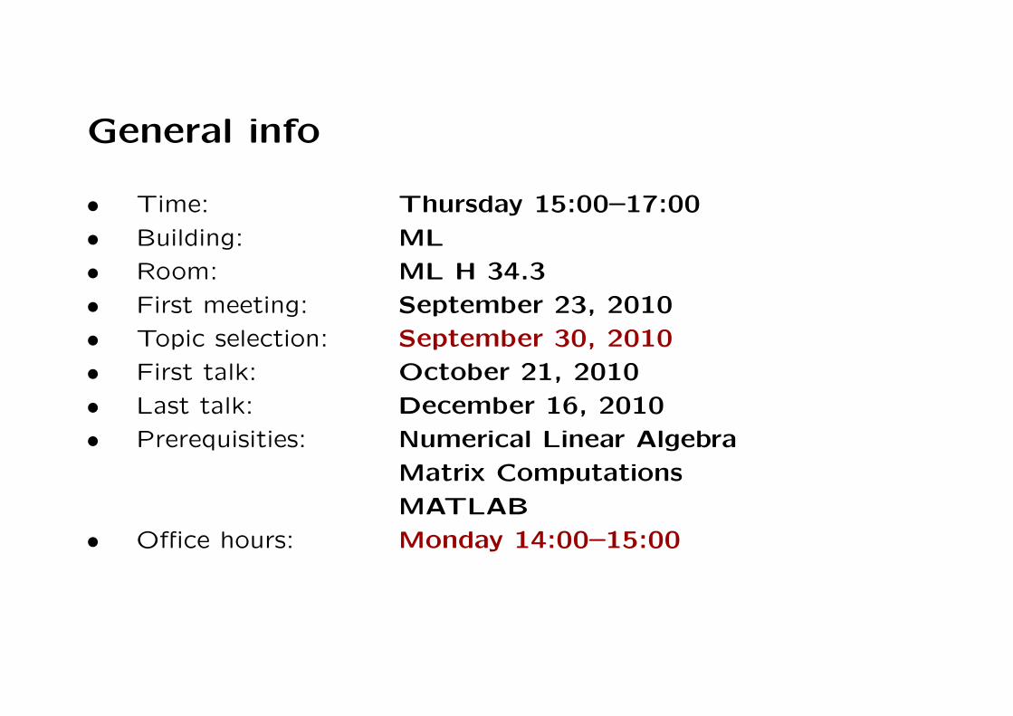
General info

• Time: Thursday 15:00–17:00

• Building: ML

• Room: ML H 34.3

• First meeting: September 23, 2010

• Topic selection: September 30, 2010

• First talk: October 21, 2010

• Last talk: December 16, 2010

• Prerequisities: Numerical Linear Algebra

Matrix Computations

MATLAB

• Office hours: Monday 14:00–15:00

What do I have to do?

• Regularly attend the seminar.• Give a successful talk about the given topic in English.

Please, meet us for consultation before the talk,– 1st approximately 2 weeks before,– 2nd approximately 3 days before.Send us the presentation slides after the talk.

• Write a short report (summary) about the topic (3 pages).

Optionally

• MATLAB task: play with simple 1D problems as well asimage deblurring.

• Implement in MATLAB some experiments from the reading material.

Send us the slides and report via e-mail.

Organization

• 2 presentations per week =⇒ 9 weeks

Timetable (Tentative)

• 1 week October 21 the first two talks bachelor st.• 2 week October 28 bachelor st.• 3 week November 04 bachelor st.• 4 week November 11 ¿an important date? BSc/MSc st.• 5 week November 18 master st.• 6 week November 25 master st.• 7 week December 02 master st.• 8 week December 09 master st.• 9 week December 16 the last two talks master st.

(recommendation only)

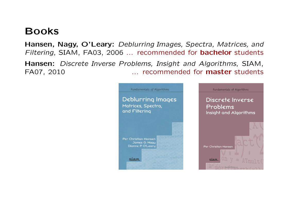
BooksHansen, Nagy, O’Leary: Deblurring Images, Spectra, Matrices, andFiltering, SIAM, FA03, 2006 ... recommended for bachelor students

Hansen: Discrete Inverse Problems, Insight and Algorithms, SIAM,FA07, 2010 ... recommended for master students

Books – availability

Legal possibilities:

• Amazon.com ($130 together, for seriously interested only ;))

• ETHZ library (the second book only)

• Privat

Other possibilities:

• Electronic (pre-version of the first book only)

• Copy

MATLAB code

We recommend:

Regularization Tools

http://www2.imm.dtu.dk/~pch/Regutools

by P. C. Hansen,

HNO package

http://www2.imm.dtu.dk/~pch/HNO

by P. C. Hansen, J. Nagy, D. O’Leary.

Google “Per Christian Hansen ” > go to “Stuff to Download ” > open

“Regularization Tools ” and “Debluring Images ”.

Manipulating images in MATLAB

What is an image?

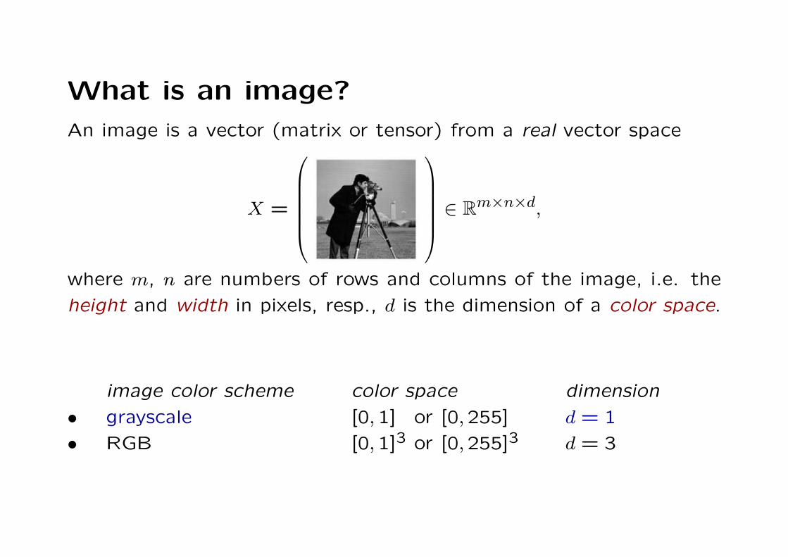
An image is a vector (matrix or tensor) from a real vector space

X =

⎛⎜⎜⎜⎜⎜⎝

⎞⎟⎟⎟⎟⎟⎠

∈ Rm×n×d,

where m, n are numbers of rows and columns of the image, i.e. the

height and width in pixels, resp., d is the dimension of a color space.

image color scheme color space dimension

• grayscale [0,1]3 or [0,255] d = 1

• RGB [0,1]3 or [0,255]3 d = 3

Image Basics

• Images can be color, grayscale or binary.

• Grayscale intensity image: 2D array where each entry

contains the intensity value of the corresponding pixel.

There are many types of image file formats:

• GIF (Graphics Interchange Format)

• JPEG (Joint Photographic Experts Group)

• PNG (Portable Network Graphics)

• TIFF (Tagged Image File Format)

Images can be also stored using the “MAT-file” format.

Reading, Displaying and Writing Images

The command imfinfo displays information about the images stored

in the data file:

info = imfinfo(’cameraman.tif’);

The command imread loads an image in MATLAB:

I = imread(’cameraman.tif’);

Images can be displayed by three commands:

imshow, imagesc, and image.

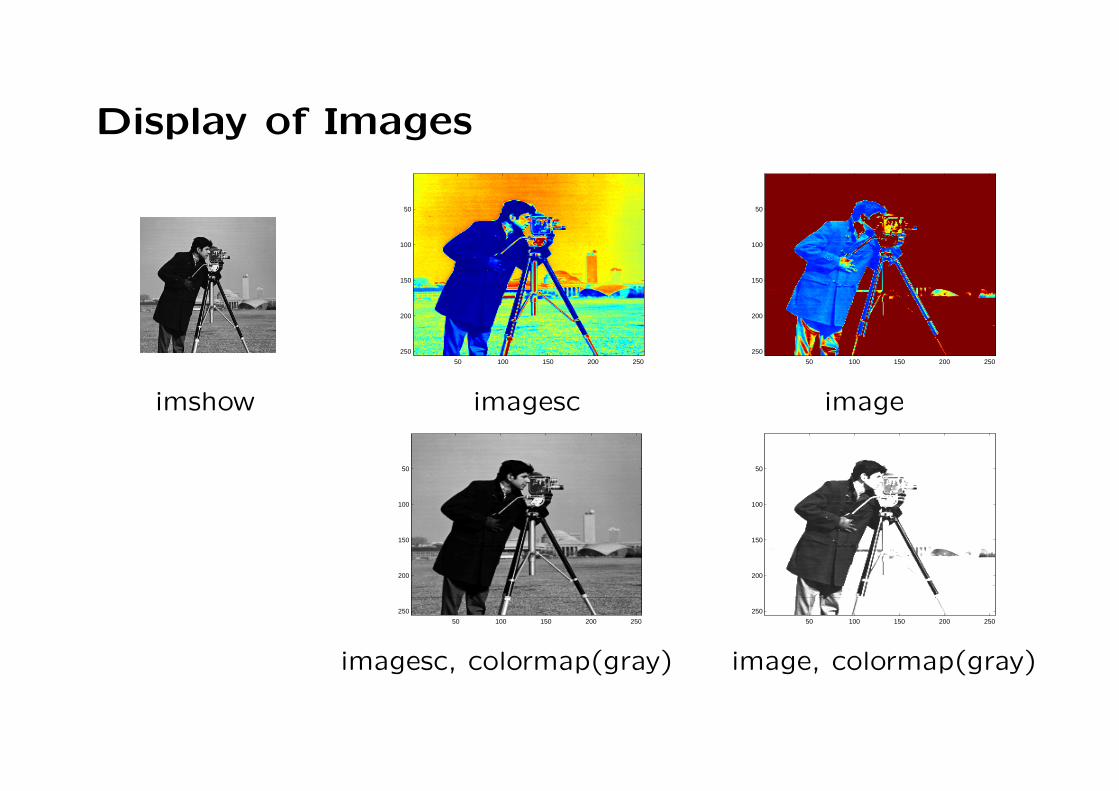
Display of Images

imshow imagesc image

50 100 150 200 250

50

100

150

200

250

50 100 150 200 250

50

100

150

200

250

imagesc, colormap(gray) image, colormap(gray)

50 100 150 200 250

50

100

150

200

250

50 100 150 200 250

50

100

150

200

250

Display of Images (cont’d)

• imshow renders images more accurately in terms of size and color

• image and imagesc display images with a false colormap

• image does not provide a proper scaling of the pixel values

• imagesc should be combined with axis image

Writing of Images

The imwrite command writes an image to a file:

imwrite(I, ’image.jpg’);

Arithmetic on Images

• Integer representation of images can be limiting.

• Common practice: convert the image to double precision,

process it, and convert it back to the original format.

• The function double does the conversion: Id = double(I);

• When the input image has double entries, imshow expects values

in [0,1].

• Use imshow(Id,[]) to avoid unexpected results!

• The function rgb2gray can be used to convert color images

to grayscale intensity images.

Summary: A very short guide to manipulat-ing images in MATLAB

X = imread(’file.bmp’); % opens an image in MATLAB

X = double(X); % converts X to doubles

% X is a standard matrix (2D array) in grayscale case

% X is a 3D array in color case, three 2D arrays (for R, G, and B)

colormap gray; % changes the color scheme in MATLAB

imshow(X); % plots the (real) matrix X as an image

imagesc(X); % ditto

% the first function is better, but available only with the

% Image Processing Toolbox.

% Convention: min(min(X)) is black, max(max(X)) is white.

Further information

• MATLAB (online) help,

• Image Processing Toolbox help,

• Chapter 2 of the first book [H., N., O’L., Deblurring Images],

• Regularization Tools Manual (available online),

• consultations.

Motivation

A gentle start

[Kjøller, Master Thesis, DTU Lyngby, 2007]

Another examples• Computer tomography (CT) maps a 3D object to � X-ray pictures,

A(·) ≡ : RM×N×K −→

�⊗j=1

Rm×n

is a mapping (not opeartor) of MNK voxels, to �-times mn pixels.

Boundary problem, from real analysis we know that it is (under someassumptions) uniquely solvable. In numerical computations (roundingerrors, other sources of noise, e.g. electronic noise on semiconductorsPN-junctions in transistors) it is difficult to solve (Medicine).

We lose some important information.

• Transmision tomography in crystalographics is used, e.g., for re-construction of orientation-distribution-function (ODF) of grains in a

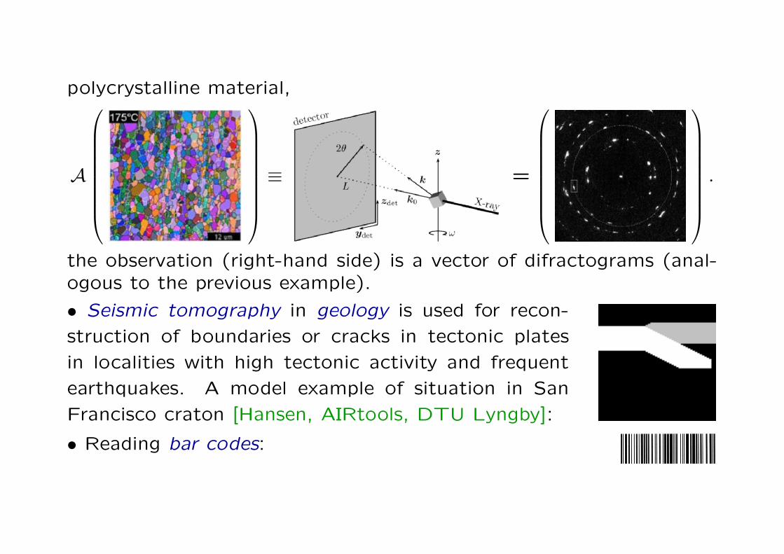
polycrystalline material,

A

⎛⎜⎜⎜⎜⎜⎜⎜⎜⎝

⎞⎟⎟⎟⎟⎟⎟⎟⎟⎠

≡ =

⎛⎜⎜⎜⎜⎜⎜⎜⎜⎝

⎞⎟⎟⎟⎟⎟⎟⎟⎟⎠

.

the observation (right-hand side) is a vector of difractograms (anal-ogous to the previous example).

• Seismic tomography in geology is used for recon-

struction of boundaries or cracks in tectonic plates

in localities with high tectonic activity and frequent

earthquakes. A model example of situation in San

Francisco craton [Hansen, AIRtools, DTU Lyngby]:

• Reading bar codes:

A brief introduction to imagedeblurring

Linear operators on a vector space Rm×n×d

Consider for simplicity the grayscale color scheme, thus d = 1.

A simple linear operator

A(X) = B, X, B ∈ Rm×n (real matrices)

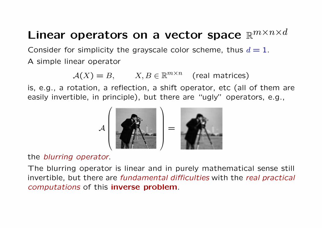
is, e.g., a rotation, a reflection, a shift operator, etc (all of them areeasily invertible, in principle), but there are “ugly” operators, e.g.,

A

⎛⎜⎜⎜⎜⎜⎝

⎞⎟⎟⎟⎟⎟⎠

=

the blurring operator.

The blurring operator is linear and in purely mathematical sense stillinvertible, but there are fundamental difficulties with the real practicalcomputations of this inverse problem.

Naive solution of an equation with the blur-ring operatorSince the operator is linear we can rewrite the problem as a systemof linear algebraic equations

Ax = b, A ∈ Rnm×nm, x, b ∈ R

nm

and solve it: True x and blured b image, and naive solution A−1b: x = true image

,

b = blurred, noisy image

,

x = inverse solution

,(example by James Nagy, Emory University, Atlanta).

Question: What did it happen ???

Blurring operator – Gaußian blur

The simplest case is the Gaußian blurring operator (used in the pre-vious example).

First recall the Gauß function in 1D and 2D:

−3 −2 −1 0 1 2 3

0

0.5

1

1.5

−4

−2

0

2

4

−4

−2

0

2

4

0

0.5

1

1.5

f1D(k) = e−k2f2D(h, w) = e−(h2+w2)

Note that the 2D Gauß function is separable, i.e. can be written as a product of

two functions of one variable f2D(h, w) = e−(h2+w2) = e−h2

e−w2

= f1D(h)f1D(w).

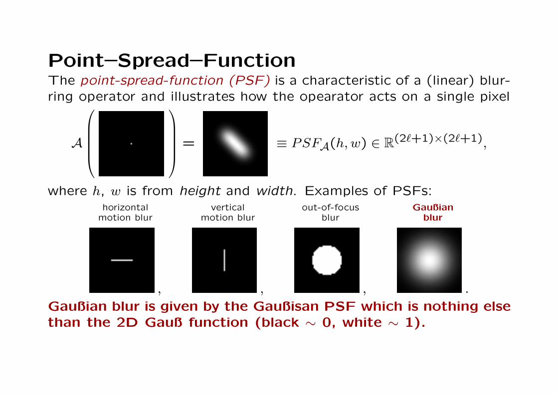
Point–Spread–FunctionThe point-spread-function (PSF) is a characteristic of a (linear) blur-ring operator and illustrates how the opearator acts on a single pixel

A

⎛⎜⎜⎜⎜⎝

⎞⎟⎟⎟⎟⎠ = ≡ PSFA(h, w) ∈ R

(2�+1)×(2�+1),

where h, w is from height and width. Examples of PSFs:horizontal vertical out-of-focus Gaußian

motion blur motion blur blur blur

, , , .

Gaußian blur is given by the Gaußisan PSF which is nothing elsethan the 2D Gauß function (black ∼ 0, white ∼ 1).

Relatioship between A and PSFAThe PSF construction from the operator A(·) =⇒ PSFA(w, h) is clearfrom the previous slide.

The (grayscale) image can be represented as a 2D function X =X(w, h) = xw,h (color of the pixel at position (w, h)), the action of Acan be obtained by the 2D convolution of X with the PSFA.

In (our) discrete and finite case, recall that

X ∈ Rm×n, PSFA ∈ R

(2�+1)×(2�+1)

are matrices, it is

A(X) =�∑

η=−�

�∑ν=−�

X(w − ν, h − η)PSFA(� + 1 + ν, � + 1 + η).

Problem: Entries xw,h are not defined for w = −� + 1, . . . ,0, andm + 1, . . . , m + � and w = −� + 1, . . . ,0, and n + 1, . . . , n + � !!!

Question: Is it possible to construct the matrix A from the PSF ???

Boundary conditions

The action of the (inverse) operator is not defined close to boundaryof the image. There are several possibilities, typically:

zero boundary periodic boundary reflexive boundary

which involve structure of the matrix in the linear system.

Boundary conditions – 1D problemPSF is a Toplitz matrix

b ≡

⎡⎢⎢⎢⎢⎢⎢⎣

b1b2b3b4b5

⎤⎥⎥⎥⎥⎥⎥⎦

=

⎡⎢⎢⎢⎢⎢⎢⎣

p3 p2 p1p4 p3 p2 p1p5 p4 p3 p2 p1

p5 p4 p3 p2p5 p4 p3

⎤⎥⎥⎥⎥⎥⎥⎦

⎡⎢⎢⎢⎢⎢⎢⎣

x1x2x3x4x5

⎤⎥⎥⎥⎥⎥⎥⎦≡ APSF x,

with the boundary condition⎡⎢⎢⎢⎢⎢⎢⎣

b1b2b3b4b5

⎤⎥⎥⎥⎥⎥⎥⎦

=

⎡⎢⎢⎢⎢⎢⎢⎣

p5 p4 p3 p2 p1p5 p4 p3 p2 p1

p5 p4 p3 p2 p1p5 p4 p3 p2 p1

p5 p4 p3 p2 p1

⎤⎥⎥⎥⎥⎥⎥⎦

⎡⎢⎢⎢⎢⎢⎢⎣

??x??

⎤⎥⎥⎥⎥⎥⎥⎦

.

Note: The row [p1, p2, p3, p4, p5] is, e.g., the discretized 1D Gauß function f1D(k).

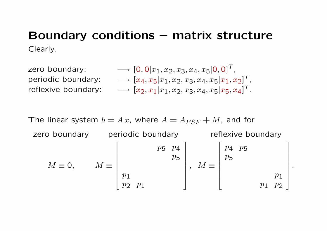
Boundary conditions – matrix structureClearly,

zero boundary: −→ [0,0|x1, x2, x3, x4, x5|0,0]T ,periodic boundary: −→ [x4, x5|x1, x2, x3, x4, x5|x1, x2]

T ,reflexive boundary: −→ [x2, x1|x1, x2, x3, x4, x5|x5, x4]

T .

The linear system b = A x, where A = APSF + M , and for

zero boundary periodic boundary reflexive boundary

M ≡ 0, M ≡

⎡⎢⎢⎢⎢⎢⎢⎣

p5 p4p5

p1p2 p1

⎤⎥⎥⎥⎥⎥⎥⎦

, M ≡

⎡⎢⎢⎢⎢⎢⎢⎣

p4 p5p5

p1p1 p2

⎤⎥⎥⎥⎥⎥⎥⎦

.

Back to the naive solutionThere are fundamental difficulties with solving the linear problem:

• Action of the blurring operator A is realized by convolution with verysmooth 2D Gauß function, the operator has a smoothing property.

• The (example) right-hand side B is represented by smooth function.

• While solving the linear system, i.e. evaluation A−1(B), we invert asmoothing operator, apply it on a smooth function, and we want toobtain an image X which is typically discontiuous function. Recall

B =

b = blurred, noisy image

, X =

x = true image

.

Inverse problems ≡ Troubles!• The problem is typically very sensitive to small perturbations (e.g.,

smooth B, smooth A, nonsmooth solution).

• But B is always corrupted by rounding errors (noise). Thus we have

system of equations

Ax = b + eexact, where e ∈ Rmn is unknown,

and we want to find xtrue ≡ A−1b. The naive solution ilustrates the

catastophical impact of noise

Xnaive ≡ A−1(Bexact + E) =

x = inverse solution

.

Instead of the solution we see the amplified noise only.

• Condition number of A is very large, e.g. κ(A) ≈ 10100, i.e. A is

close to singular, we can easily lose some important information.

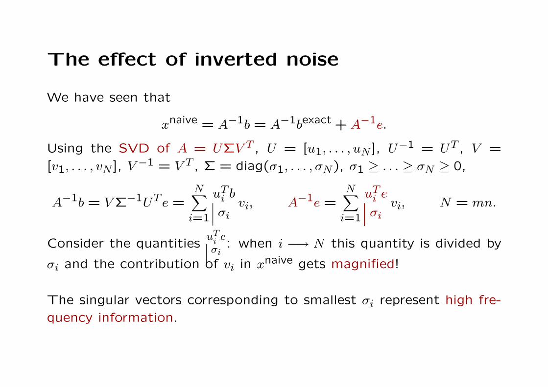
The effect of inverted noise

We have seen that

xnaive = A−1b = A−1bexact + A−1e.

Using the SVD of A = UΣV T , U = [u1, . . . , uN ], U−1 = UT , V =

[v1, . . . , vN ], V −1 = V T , Σ = diag(σ1, . . . , σN), σ1 ≥ . . . ≥ σN ≥ 0,

A−1b = V Σ−1UTe =N∑

i=1

uTi b

σivi, A−1e =

N∑i=1

uTi e

σivi, N = mn.

Consider the quantitiesuT

i eσi

: when i −→ N this quantity is divided by

σi and the contribution of vi in xnaive gets magnified!

The singular vectors corresponding to smallest σi represent high fre-

quency information.

The effect of inverted noise — SVD

0 10 20 30 40 50 60

10−40

10−30

10−20

10−10

100

j

σj

|u*jb

e|

|u*jb

s|

Don’t panic!

We have a plan B!Using “clever” methods (regularization, spectral filtering) survive theproblem

B =

b = blurred, noisy image

−→ Xapprox =

659 iterations

.

Main idea of regularization methods: Filter out the components cor-responding to the small σi.

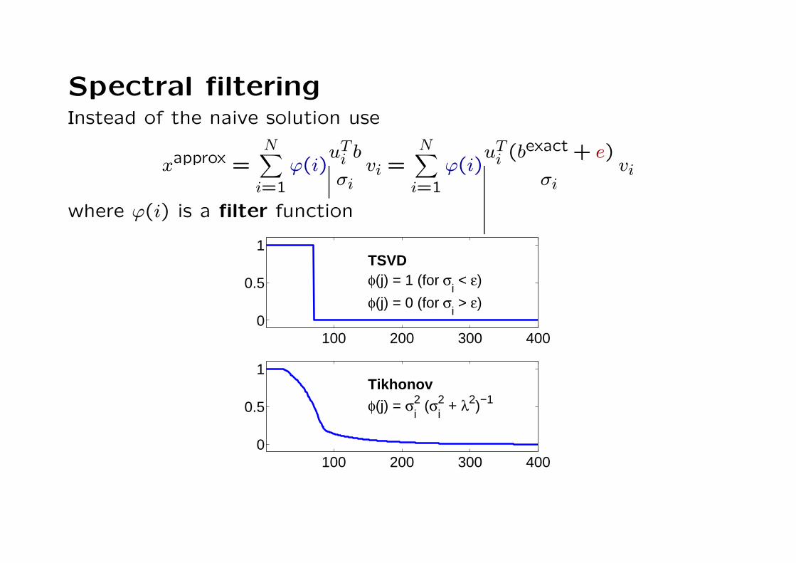
Spectral filteringInstead of the naive solution use

xapprox =N∑

i=1

ϕ(i)uT

i b

σivi =

N∑i=1

ϕ(i)uT

i (bexact + e)

σivi

where ϕ(i) is a filter function

100 200 300 4000

0.5

1TSVDφ(j) = 1 (for σ

i < ε)

100 200 300 4000

0.5

1Tikhonovφ(j) = σ

i2 (σ

i2 + λ2)−1

φ(j) = 0 (for σi > ε)

Fredholm integral equation of the first kind

Generic form (1D):∫ 1

0K(s, t)f(t)dt = g(s), 0 ≤ s ≤ 1.

Inverse problem: Given the “kernel” K and g, compute f

(typically g is smooth and f has discontinuities!)

Deconvolution problem: special case of the above∫ 1

0h(s − t)f(t)dt = g(s), 0 ≤ s ≤ 1.

Singular value expansion (SVE) of K: Important analysis tool.

Reading assignments topics

See the list of topics.