Investigating a Physically­Based Signal Power Model 

for Robust Low Power Wireless Link Simulation

Philip Levispal@cs.stanford.edu

Computer Systems

Laboratory

Stanford University

Tal Rusaktr76@cornell.edu

Department of

Computer Science

Cornell University

2

Outline

• Introduction

• Phase correction and signal extrapolation

• Validation and Evaluation

• Conclusion

3

Low Power Wireless Link Performance Is Poor

• Protocols for sensor networks are carefully designed and heavily simulated

• Packet yield in real deployments is low:

– Volcano Study: 68% [ESWN 05]

– Great Duck Island: 58% [SenSys 04]

– Redwood Study: 40% [SenSys 05]

– Potato Agriculture Study: 2% [WPDRTS 06]

• Low packet yield leads to loss of information from networks

4

Wireless Link Simulation

• Analytical Models

– For example, Path Loss and Shadowing Model [ICEE 06]

– Many assume packet reception independence

• Empirical Models 

– Packet receptions and losses are not temporally independent

– Noise+Interference modeled using CPM [IPSN 07]

5

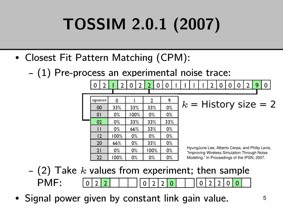
TOSSIM 2.0.1 (2007)

• Closest Fit Pattern Matching (CPM):

– (1) Pre­process an experimental noise trace:

– (2) Take k values from experiment; then sample PMF:

• Signal power given by constant link gain value.

k = History size = 2

HyungJune Lee, Alberto Cerpa, and Philip Levis, "Improving Wireless Simulation Through Noise Modeling." In Proceedings of the IPSN, 2007.

6

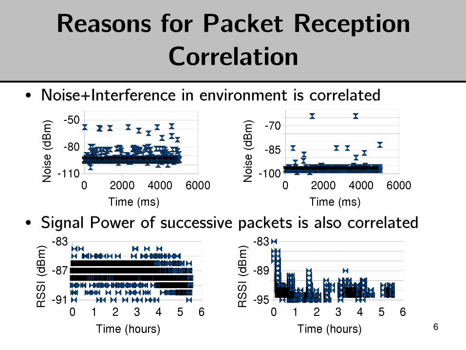
Reasons for Packet Reception Correlation

• Noise+Interference in environment is correlated

• Signal Power of successive packets is also correlated

7

Physically Modeling Signal Power

• Idea: Collect a signal power trace and use CPM to model signal power.

• Collecting power traces is more complex than collecting noise traces, since: 

– Signal power is a property of a pair of nodes in the network

– Signal power can only be approximated by sampling the RSSI register, which actually reports signal+noise, where wave phases are considered

– If a packet is lost in transmission, then even the RSSI estimate is not possible.

8

Contributions

• We suggest solutions to major challenges in modeling signal power:

– Correcting for phase

– Two algorithms for extrapolating from lossy traces: Average Value and Expected Value

• Our algorithms improve simulation substantially:

– PRR simulated to within 22% absolute difference

– Methods reduce KW distance of simulations by 66% compared to current approaches

9

Outline

• Introduction

• Phase correction and signal extrapolation

• Validation and Evaluation

• Conclusion

10

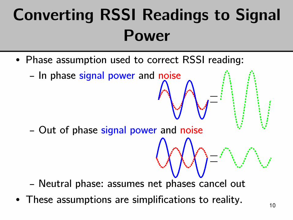
Converting RSSI Readings to Signal Power

• Phase assumption used to correct RSSI reading:

– In phase signal power and noise

– Out of phase signal power and noise 

– Neutral phase: assumes net phases cancel out

• These assumptions are simplifications to reality.

11

Algorithm for Filling­In Lossy Signal Power Links

• Two algorithms suggested:

– Fill in average value for all missing values

– Compute expected distribution of missing signal power values over the whole trace and then sample the distribution

12

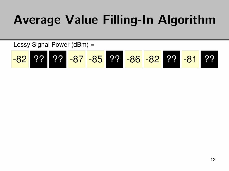
Average Value Filling­In Algorithm

Lossy Signal Power (dBm) =

­82 ?? ?? ­87 ­85 ?? ­86 ­82 ?? ­81 ??

13

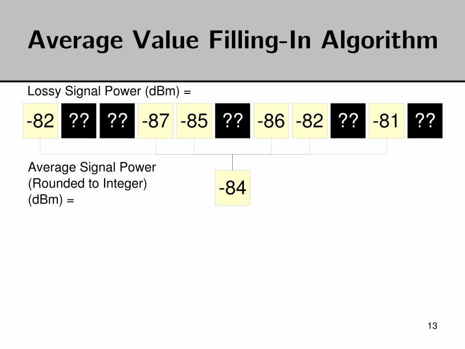
Average Value Filling­In Algorithm

Lossy Signal Power (dBm) =

­82 ?? ?? ­87 ­85 ?? ­86 ­82 ?? ­81 ??

Average Signal Power(Rounded to Integer) (dBm) =

­84

14

Average Value Filling­In Algorithm

Lossy Signal Power (dBm) =

­82 ?? ?? ­87 ­85 ?? ­86 ­82 ?? ­81 ??

Filled­In Signal Power (dBm) =

­82 ­84 ­84 ­87 ­85 ­84 ­86 ­82 ­84 ­81 ­84

Average Signal Power(Rounded to Integer) (dBm) =

­84

15

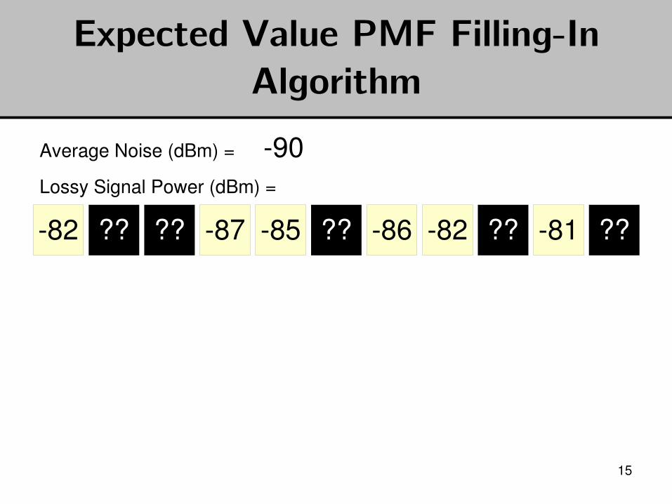
Expected Value PMF Filling­In Algorithm

Average Noise (dBm) =       ­90 Lossy Signal Power (dBm) =

­82 ?? ?? ­87 ­85 ?? ­86 ­82 ?? ­81 ??

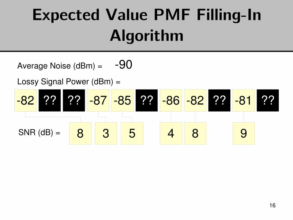
16

Expected Value PMF Filling­In Algorithm

Average Noise (dBm) =       ­90 Lossy Signal Power (dBm) =

­82 ?? ?? ­87 ­85 ?? ­86 ­82 ?? ­81 ??

SNR (dB) = 8 3 5 4 98

17

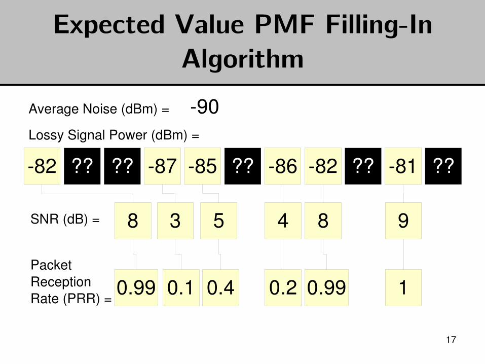
Expected Value PMF Filling­In Algorithm

Average Noise (dBm) =       ­90 Lossy Signal Power (dBm) =

­82 ?? ?? ­87 ­85 ?? ­86 ­82 ?? ­81 ??

SNR (dB) = 8 3 5 4 98

PacketReceptionRate (PRR) =

0.99 0.1 0.4 0.2 10.99

18

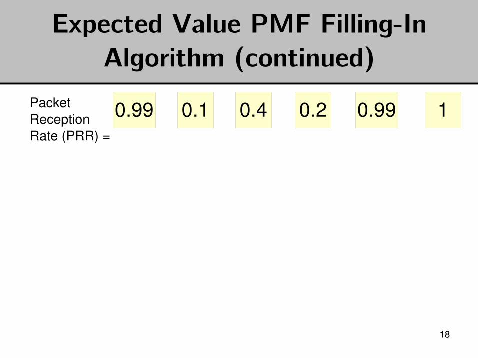
Expected Value PMF Filling­In Algorithm (continued)

PacketReceptionRate (PRR) =

0.99 0.1 0.4 0.2 10.99

19

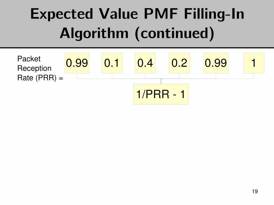
Expected Value PMF Filling­In Algorithm (continued)

PacketReceptionRate (PRR) =

0.99 0.1 0.4 0.2 10.99

1/PRR ­ 1

20

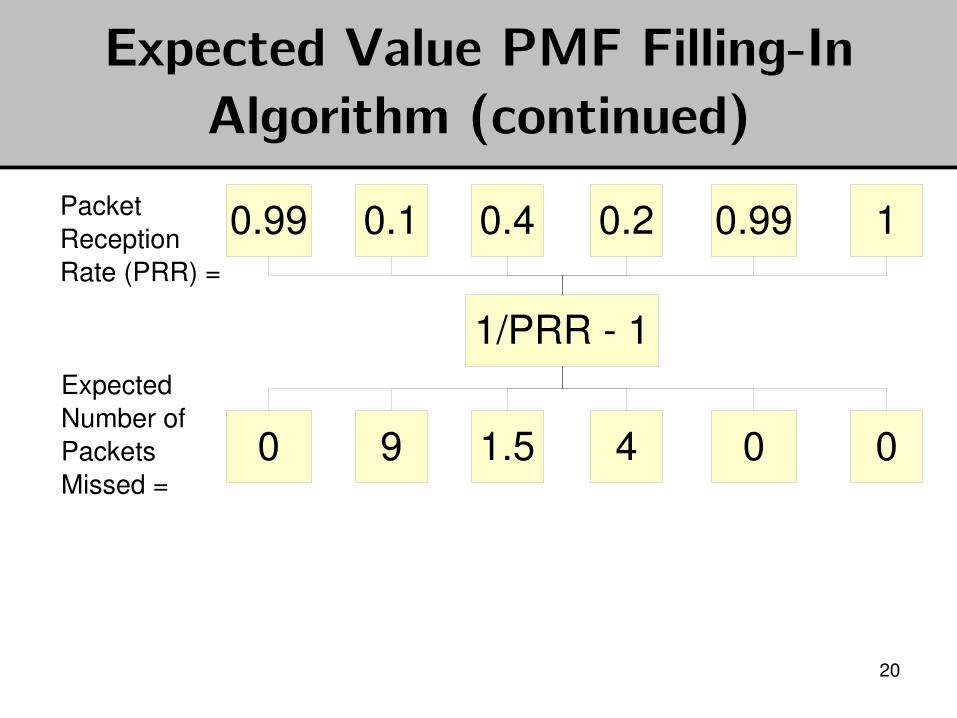
Expected Value PMF Filling­In Algorithm (continued)

PacketReceptionRate (PRR) =

0.99 0.1 0.4 0.2 10.99

1/PRR ­ 1

0 9 1.5 4 00

Expected Number of Packets Missed =

21

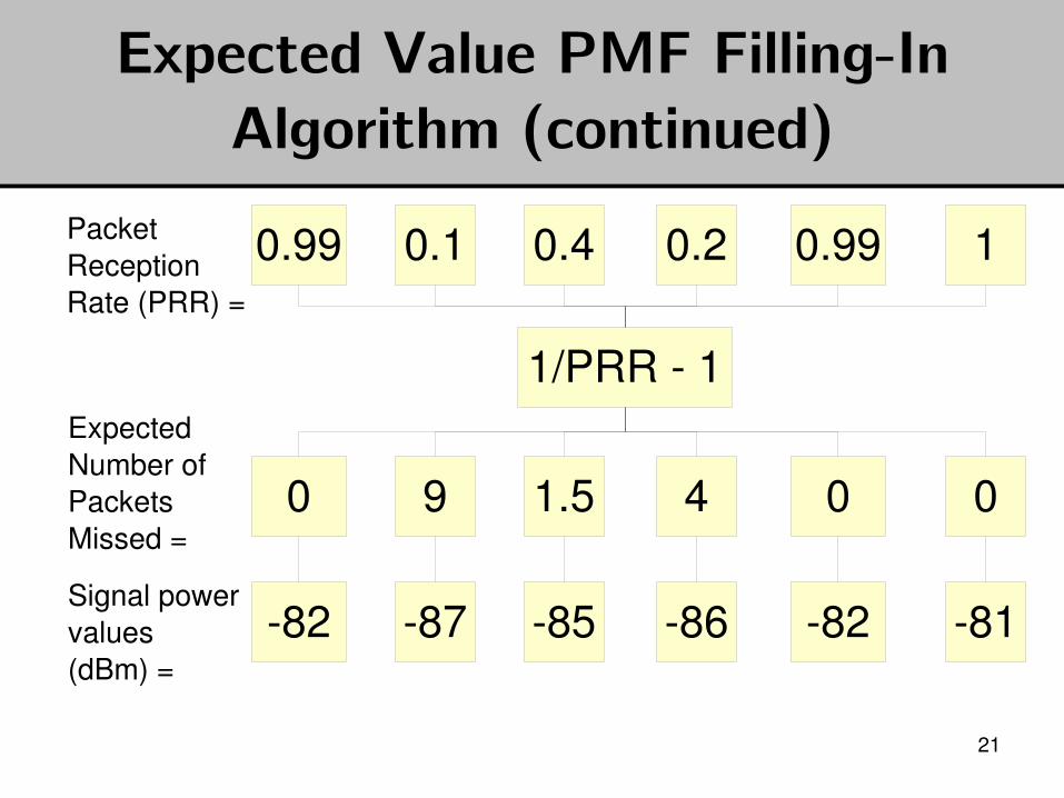
Expected Value PMF Filling­In Algorithm (continued)

PacketReceptionRate (PRR) =

0.99 0.1 0.4 0.2 10.99

1/PRR ­ 1Expected Number of Packets Missed =

0 9 1.5 4 00

­82 ­87 ­85 ­86 ­81­82Signal power values (dBm) =

22

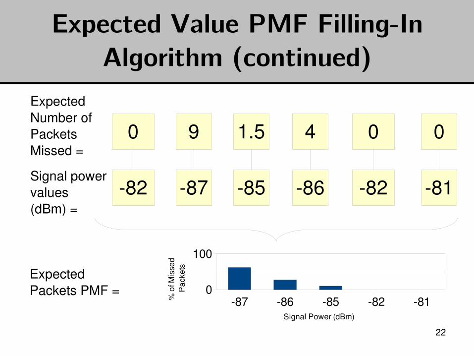
Expected Value PMF Filling­In Algorithm (continued)

Expected Packets PMF =

­87 ­86 ­85 ­82 ­810

100

Signal Power (dBm)

% o

f Mis

sed 

Pac

kets

Expected Number of Packets Missed =

0 9 1.5 4 00

­82 ­87 ­85 ­86 ­81­82Signal power values (dBm) =

23

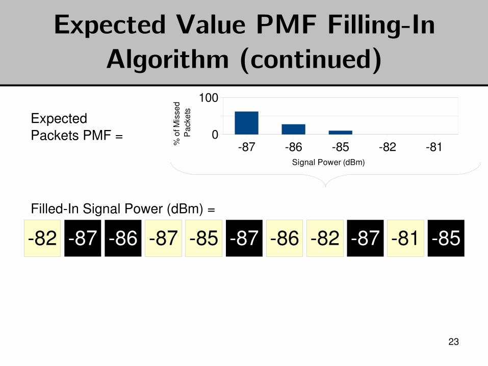
Expected Value PMF Filling­In Algorithm (continued)

Filled­In Signal Power (dBm) =

­82 ­87 ­86 ­87 ­85 ­87 ­86 ­82 ­87 ­81 ­85

Expected Packets PMF =

­87 ­86 ­85 ­82 ­810

100

Signal Power (dBm)

% o

f Mis

sed 

Pac

kets

24

Outline

• Introduction

• Phase correction and signal extrapolation

• Validation and Evaluation

• Conclusion

25

Validation

• Goal is to correctly simulate a particular link between to nodes

• It is possible to use experiments to validate this simulation method

• Conducted packet delivery experiments at 4 Hz for 12 hours at various locations on the Cornell University Campus.

• 4 Hz frequency chosen as a baseline: future work will investigate different collection frequencies and the impacts on the results.

26

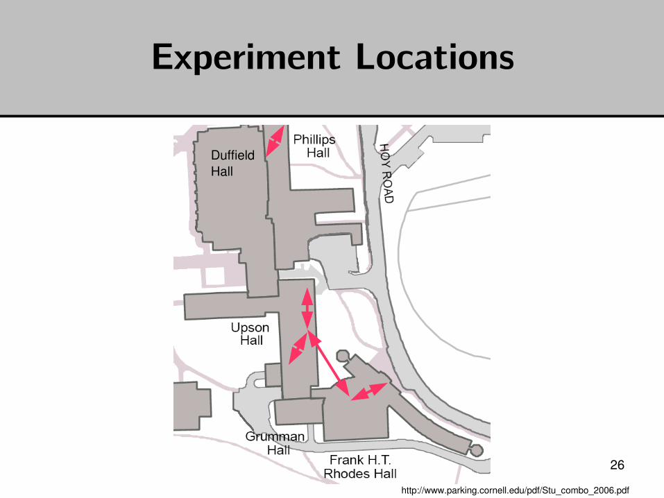
Experiment Locations

http://www.parking.cornell.edu/pdf/Stu_combo_2006.pdf

Duffield  Hall

27

Evaluation Criteria

• Packet Reception Rate (PRR)

– First order parameter, difficult to get right in general wireless simulators

• Kantorovich­Wasserstein (KW) distance on Conditional Packet Delivery Functions (CPDFs)

– Rigorous measure of the similarity between two distributions, which places more emphasis on rare rather than common case

– Captures packet burstiness at the level of individual packets.

28

0.426 0.591 0.672 0.7550.000.050.100.150.200.250.300.350.400.450.50

In PhaseNo CorrectionOut of PhaseTOSSIM 2.0.2 

Experimental PRR

|Exp

erim

enta

l PR

R ­

 Sim

ulat

ed P

RR

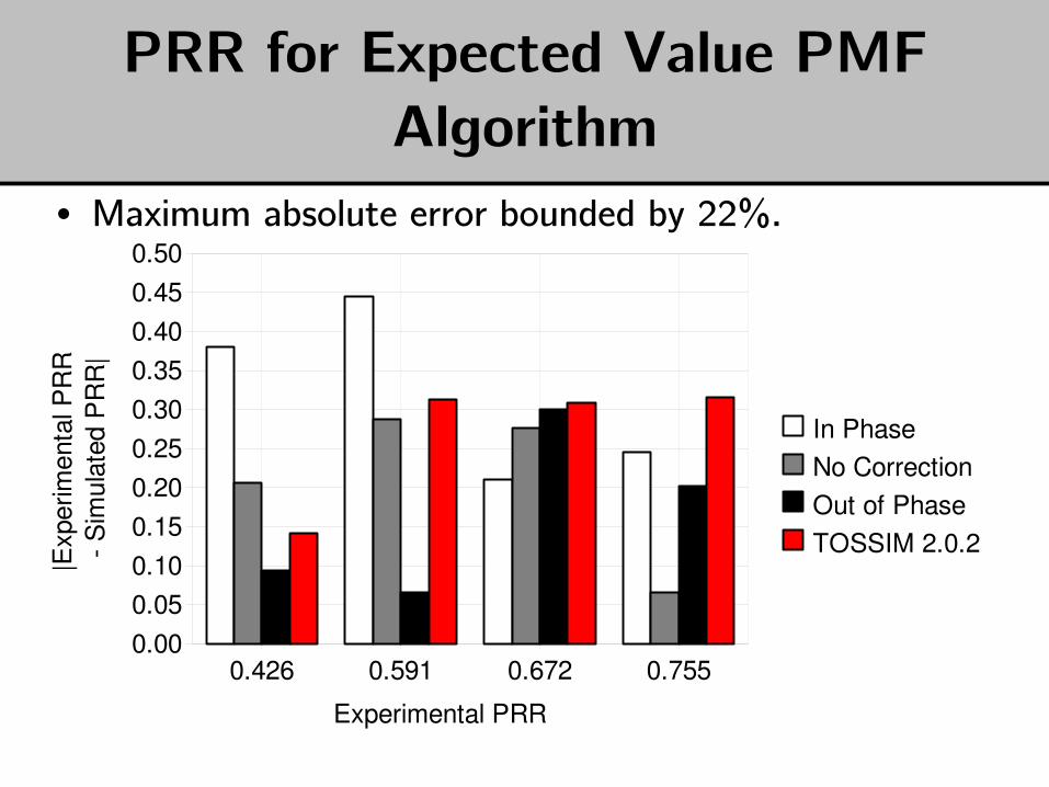
|PRR for Expected Value PMF 

Algorithm• Maximum absolute error bounded by 22%.

29

0.426 0.591 0.672 0.7550.000.050.100.150.200.250.300.350.400.450.50

In PhaseNo CorrectionOut of PhaseTOSSIM 2.0.2 

Experimental PRR

|Exp

erim

enta

l PR

R ­

 Sim

ulat

ed P

RR

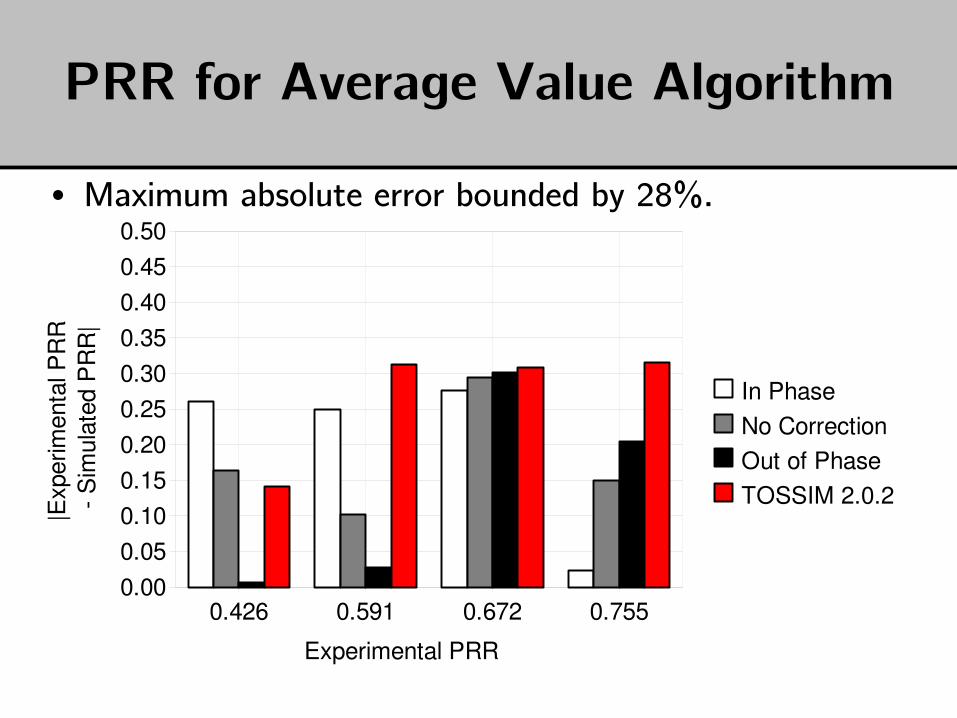
|PRR for Average Value Algorithm

• Maximum absolute error bounded by 28%.

30

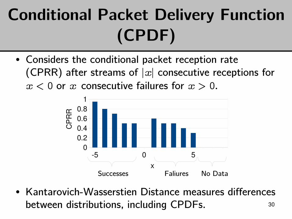
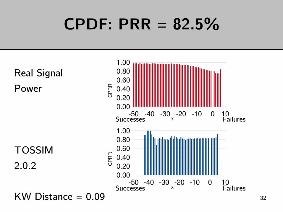
Conditional Packet Delivery Function (CPDF)

• Considers the conditional packet reception rate (CPRR) after streams of |x| consecutive receptions for x < 0 or x consecutive failures for x > 0.

• Kantarovich­Wasserstien Distance measures differences between distributions, including CPDFs.

­5 0 50

0.20.40.60.8

1

x

CP

RR

Successes Faliures No Data

31

­50 ­40 ­30 ­20 ­10 0 100.000.200.400.600.801.00

x

CP

RR

­50 ­40 ­30 ­20 ­10 0 100.000.200.400.600.801.00

x

CP

RR

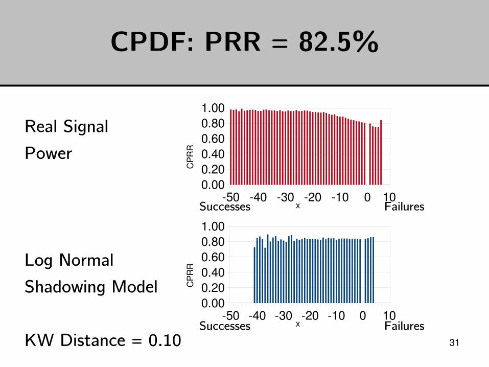
CPDF: PRR = 82.5%

Real Signal

Power

Log Normal

Shadowing Model

KW Distance = 0.10Successes Failures

Successes Failures

32

­50 ­40 ­30 ­20 ­10 0 100.000.200.400.600.801.00

x

CP

RR

­50 ­40 ­30 ­20 ­10 0 100.000.200.400.600.801.00

x

CP

RR

CPDF: PRR = 82.5%

Real Signal

Power

TOSSIM

2.0.2

KW Distance = 0.09Successes Failures

Successes Failures

33

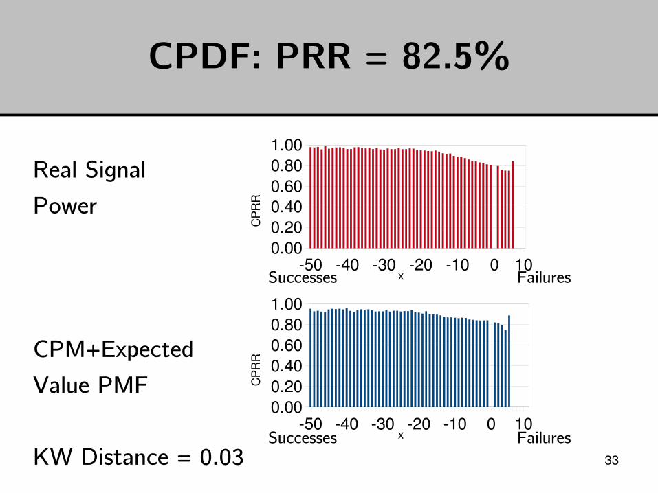
­50 ­40 ­30 ­20 ­10 0 100.000.200.400.600.801.00

x

CP

RR

­50 ­40 ­30 ­20 ­10 0 100.000.200.400.600.801.00

x

CP

RR

CPDF: PRR = 82.5%

Real Signal

Power

CPM+Expected 

Value PMF

KW Distance = 0.03Successes Failures

Successes Failures

34

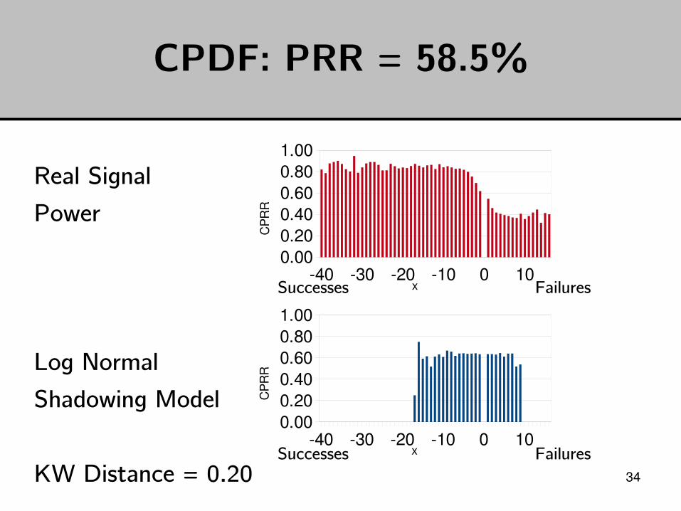
CPDF: PRR = 58.5%

­40 ­30 ­20 ­10 0 100.000.200.400.600.801.00

x

CP

RR

­40 ­30 ­20 ­10 0 100.000.200.400.600.801.00

x

CP

RR

Real Signal

Power

Log Normal 

Shadowing Model

KW Distance = 0.20Successes Failures

Successes Failures

35

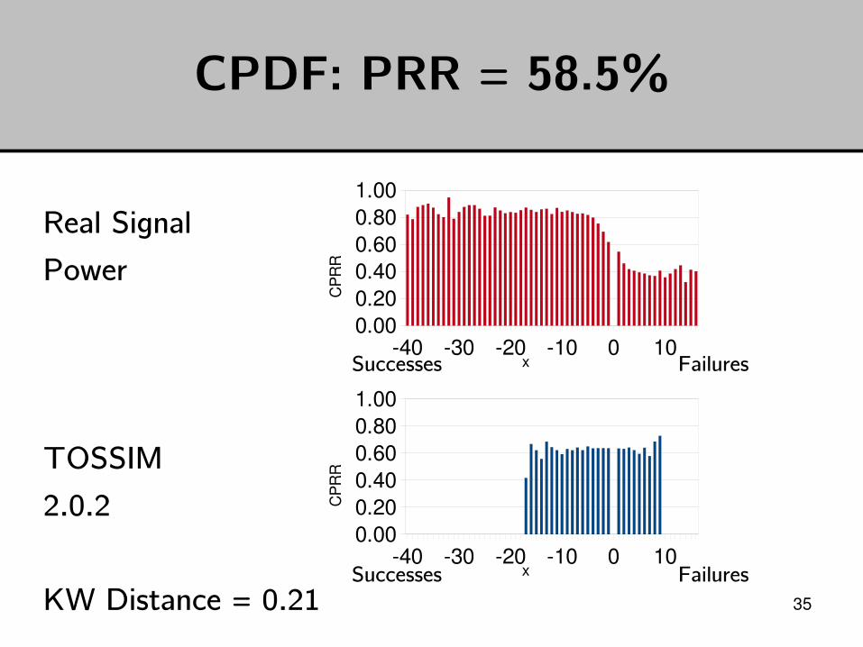
­40 ­30 ­20 ­10 0 100.000.200.400.600.801.00

x

CP

RR

CPDF: PRR = 58.5%

Real Signal

Power

TOSSIM

2.0.2

KW Distance = 0.21

­40 ­30 ­20 ­10 0 100.000.200.400.600.801.00

x

CP

RR

Successes Failures

Successes Failures

36

­40 ­30 ­20 ­10 0 100.000.200.400.600.801.00

x

CP

RR

CPDF: PRR = 58.5%

Real Signal

Power

CPM+Expected 

Value PMF

KW Distance = 0.06

­40 ­30 ­20 ­10 0 100.000.200.400.600.801.00

x

CP

RR

Successes Failures

Successes Failures

37

Outline

• Introduction

• Phase correction and signal extrapolation

• Validation and Evaluation

• Conclusion

38

Conclusions and Future Work

• KW distance < 0.1 for our experiments (substantially reduced as compared to current methods)

• PRR estimated to within 22% (typically to 10%)

• As expected, different assumptions work more effectively for different experiments.

• Future work: Development of an automated optimization layer to predict the most reasonable assumptions for a given environment.

• Future work: Investigate a signal power model that considers burstiness at many time scales, not just that of an individual packet.

39

Thank you.

Questions?

tr76@cornell.edu

40

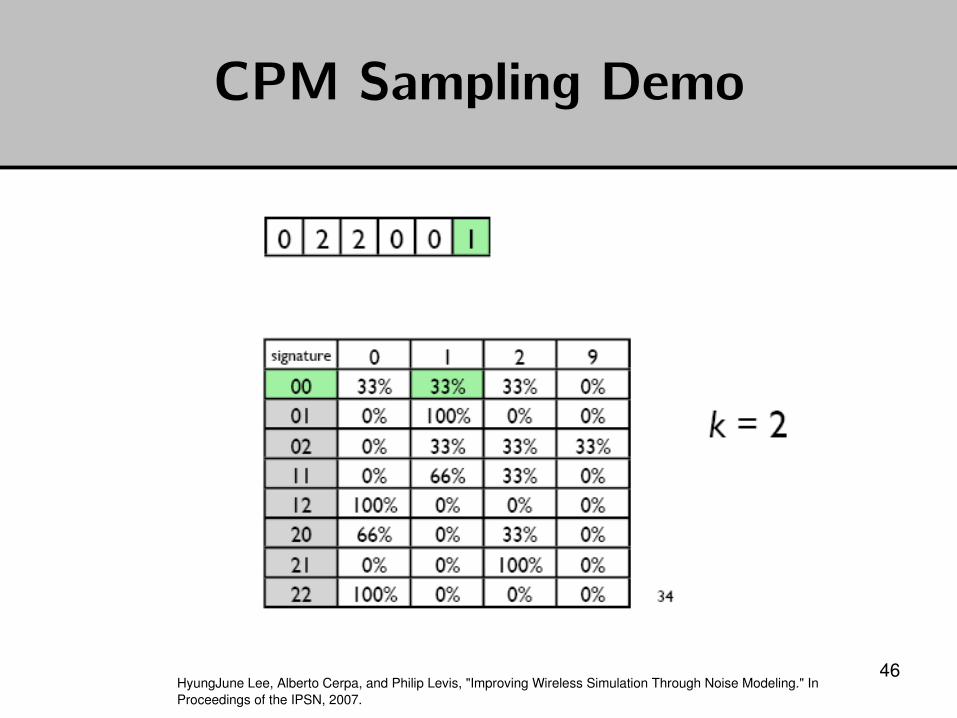
CPM Model for Trace Histories

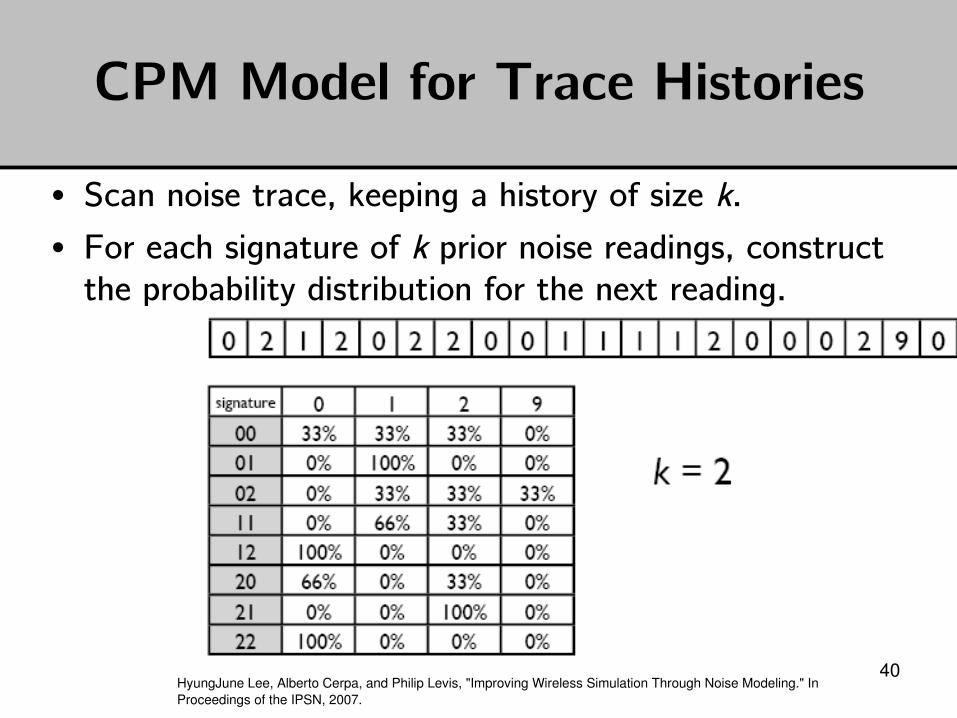
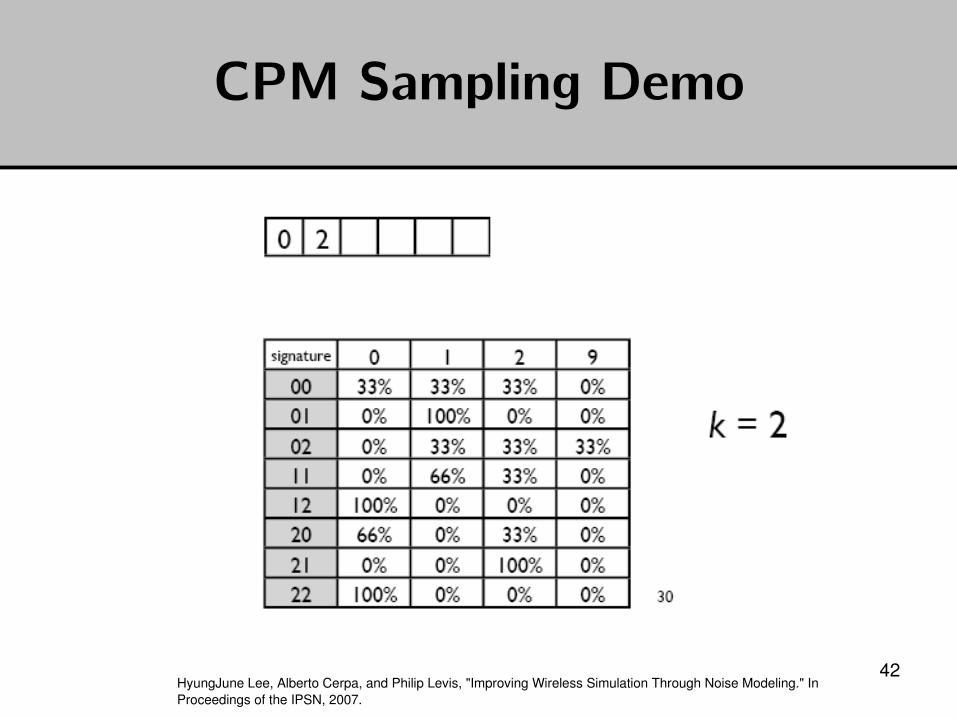
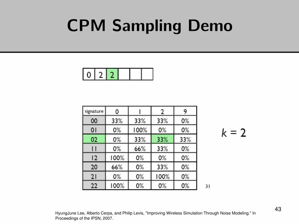
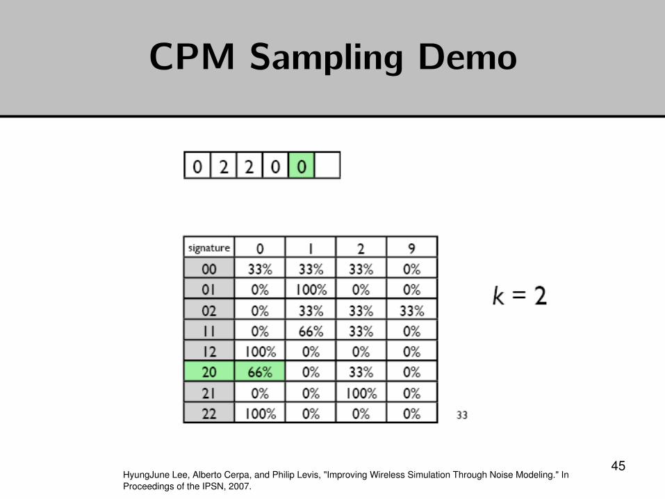
• Scan noise trace, keeping a history of size k.

• For each signature of k prior noise readings, construct the probability distribution for the next reading.

HyungJune Lee, Alberto Cerpa, and Philip Levis, "Improving Wireless Simulation Through Noise Modeling." In Proceedings of the IPSN, 2007.

41

CPM Model for Trace Histories

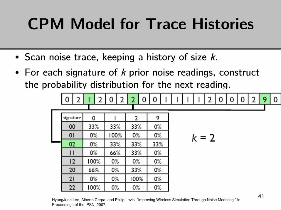
• Scan noise trace, keeping a history of size k.

• For each signature of k prior noise readings, construct the probability distribution for the next reading.

HyungJune Lee, Alberto Cerpa, and Philip Levis, "Improving Wireless Simulation Through Noise Modeling." In Proceedings of the IPSN, 2007.

42

CPM Sampling Demo

HyungJune Lee, Alberto Cerpa, and Philip Levis, "Improving Wireless Simulation Through Noise Modeling." In Proceedings of the IPSN, 2007.

43

CPM Sampling Demo

HyungJune Lee, Alberto Cerpa, and Philip Levis, "Improving Wireless Simulation Through Noise Modeling." In Proceedings of the IPSN, 2007.

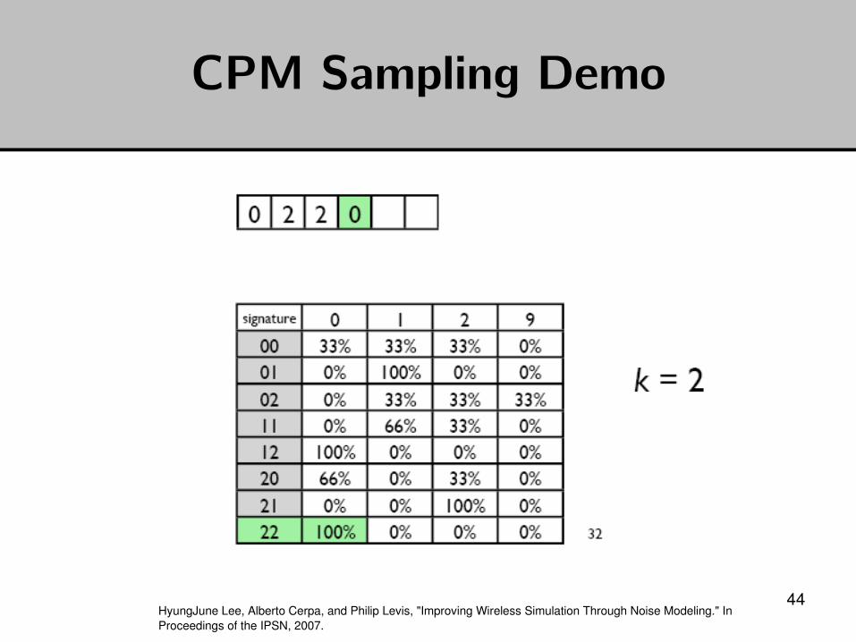
44

CPM Sampling Demo

HyungJune Lee, Alberto Cerpa, and Philip Levis, "Improving Wireless Simulation Through Noise Modeling." In Proceedings of the IPSN, 2007.

45

CPM Sampling Demo

HyungJune Lee, Alberto Cerpa, and Philip Levis, "Improving Wireless Simulation Through Noise Modeling." In Proceedings of the IPSN, 2007.

46

CPM Sampling Demo

HyungJune Lee, Alberto Cerpa, and Philip Levis, "Improving Wireless Simulation Through Noise Modeling." In Proceedings of the IPSN, 2007.

47

CPM Sampling Result

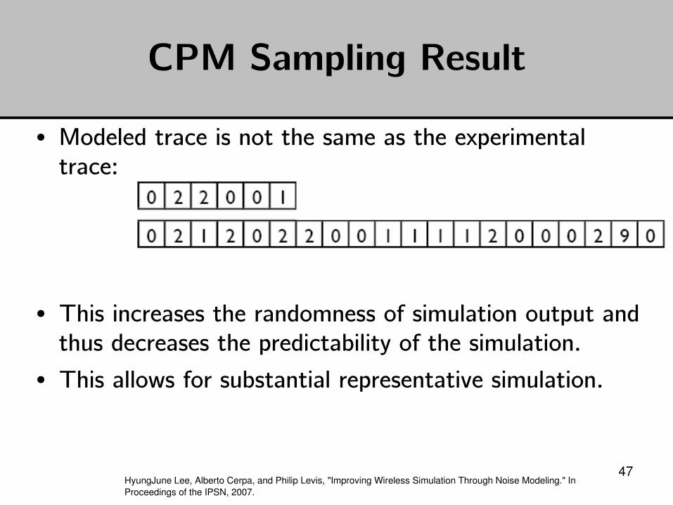
• Modeled trace is not the same as the experimental trace:

• This increases the randomness of simulation output and thus decreases the predictability of the simulation.

• This allows for substantial representative simulation.

HyungJune Lee, Alberto Cerpa, and Philip Levis, "Improving Wireless Simulation Through Noise Modeling." In Proceedings of the IPSN, 2007.