Investigating Galaxy Evolution and Active Galactic Nucleus Feedback with the

Sunyaev-Zel’dovich Effect

by

Alexander Edward Spacek

A Dissertation Presented in Partial Fulfillmentof the Requirements for the Degree

Doctor of Philosophy

Approved June 2017 by theGraduate Supervisory Committee:

Evan Scannapieco, ChairJudd Bowman

Nat ButlerChris GroppiPatrick Young

ARIZONA STATE UNIVERSITY

August 2017

ABSTRACT

Galaxy formation is a complex process with aspects that are still very uncertain or

unknown. A mechanism that has been utilized in simulations to successfully resolve

several of these outstanding issues is active galactic nucleus (AGN) feedback. Recent

work has shown that a promising method for directly measuring this energy is by

looking at small increases in the energy of cosmic microwave background (CMB)

photons as they pass through ionized gas, known as the thermal Sunyaev-Zel’dovich

(tSZ) effect.

In this work, I present stacked CMB measurements of a large number of elliptical

galaxies never before measured using this method. I split the galaxies into two redshift

groups, “low-z” for z=0.5-1.0 and “high-z” for z=1.0-1.5. I make two independent

sets of CMB measurements using data from the South Pole Telescope (SPT) and the

Atacama Cosmology Telescope (ACT), respectively, and I use data from the Planck

telescope to account for contamination from dust emission. With SPT I find average

thermal energies of 7.6+3.0−2.3× 1060 erg for 937 low-z galaxies, and 6.0+7.7

−6.3× 1060 erg for

240 high-z galaxies. With ACT I find average thermal energies of 5.6+5.9−5.6 × 1060 erg

for 227 low-z galaxies, and 7.0+4.7−4.4 × 1060 erg for 529 high-z galaxies.

I then attempt to further interpret the physical meaning of my observational

results by incorporating two large-scale cosmological hydrodynamical simulations, one

with (Horizon-AGN) and one without (Horizon-NoAGN) AGN feedback. I extract

simulated tSZ measurements around a population of galaxies equivalent to those used

in my observational work, with matching mass distributions, and compare the results.

I find that the SPT measurements are consistent with Horizon-AGN, falling within

0.4σ at low-z and 0.5σ at high-z, while the ACT measurements are very different

from Horizon-AGN, off by 6.9σ at low-z and 14.6σ at high-z. Additionally, the SPT

measurements are loosely inconsistent with Horizon-NoAGN, off by 1.8σ at low-z

i

but within 0.6σ at high-z, while the ACT measurements are loosely consistent with

Horizon-NoAGN (at least much more so than with Horizon-AGN), falling within 0.8σ

at low-z but off by 1.9σ at high-z.

ii

Dedicated to Amanda, Sneezy, and Flurry. They inspire all I do.

iii

ACKNOWLEDGMENTS

For all of the general work contained within this dissertation, I owe much to my

advisor, Evan Scannapieco, who has helped me with every aspect of it. I have also

been helped immensely by the other co-authors of Chapters 2 and 3: Seth Cohen,

Bhavin Joshi, and Phil Mauskopf. A special debt is also owed to Mark Richardson for

countless reasons, especially for qualifying exam help and the work done in Chapter

4. I also must thank all current and former members of my PhD committee for

their years of keeping tabs on my progress and giving me advice: Judd Bowman,

Nat Butler, Chris Groppi, Sangeeta Malhotra, Phil Mauskopf, and Patrick Young.

Obvious gratitude goes to Arizona State University, the School of Earth and Space

Exploration, and anyone within those groups who has been helpful. Enormous thanks

go to Amanda Truitt, Rick Sarmento, and Luke Probst for sharing offices with me

and for their help through insightful talks and general support. Finally, thanks to

Mike Veto for sharing a house with me for several years, Anusha Kalyan and Peter

Nguyen for sharing an office with me, George Che and Becky Jackson for late-night

homework sessions, and the rest of my fellow graduate students who I took classes

with, played games with, watched movies with, and everything else.

For my South Pole Telescope work specifically, I thank Shantanu Desai, Mariska

Kriek, Eliot Quataert, and Daniel Marrone for helpful discussions, and the anonymous

ApJ referee for very helpful comments. This work was supported by the National

Science Foundation (NSF) under grant AST14-07835. ES gratefully acknowledges

Joanne Cohn, Eliot Quataert, the UC Berkeley Theoretical Astronomy Center, and

Uros Seljak and the Lawrence Berkeley National Lab Cosmology group, for hosting

him when a lot of this work was done. I would also like to thank the Joint Space-

Science Institute for letting me present a poster of this work at the 2015 Supermassive

Black Hole Formation and Feedback conference.

iv

For my Atacama Cosmology Telescope (ACT) work specifically, I would like to

thank Arthur Kosowsky for helpful discussions. The publication makes use of data

products from the WISE, which is a joint project of UCLA, JPL, and Caltech funded

by NASA. It also makes use of data produced from SDSS-III, which was funded by the

Alfred P. Sloan Foundation, the NSF, the U.S. Department of Energy Office of Science,

and the SDSS-III Participating Institutions. Finally, I make use of data from the ACT

project, which operates in the Parque Astronomico Atacama in northern Chile under

the auspices of the Comision Nacional de Investigacion Cientıfica y Tecnologica de

Chile (CONICYT), and is funded by the NSF, Princeton University, U. Penn., and a

Canada Foundation for Innovation award to UBC. This work was supported by the

NSF under grant AST14-07835.

For my Horizon simulation work specifically, I would like to thank Julien De-

vriendt, Mark Richardson, and the University of Oxford for hosting me when a sig-

nificant part of the work was carried out. I’d also like to thank the ASU Graduate

and Professional Student Association for funding part of my travel to the United

Kingdom through their travel grant. This work has made use of the Horizon Cluster,

hosted by Institut d’Astrophysique de Paris, and data from the Horizon simulations

(horizon-simulation.org/about.html), with generous help from Stephane Rouberol.

For my life in general while completing this work, I’d like to sincerely thank

my entire extended family (aunts, uncles, cousins) for being amazing, and especially

thank my mom, dad, grandma, and grandpa for their incredible and constant support.

Infinite thanks to Amanda Truitt for literally everything, and thanks to her mom,

dad, sister, and the rest of her family for being amazing. Thanks to all my friends

for being awesome, especially Marcus Ghiasi for decades of good times. Thanks to

Sneezy and Flurry for bringing me joy. And finally, thanks to Rick and Morty, Key &

Peele, and the (American) Office for making me laugh throughout graduate school.

v

TABLE OF CONTENTS

Page

LIST OF TABLES . . . . . . . . . . . . . . . . . . . . . . . . . . . . . . . . . . . . . . . . . . . . . . . . . . . . . . . . . ix

LIST OF FIGURES . . . . . . . . . . . . . . . . . . . . . . . . . . . . . . . . . . . . . . . . . . . . . . . . . . . . . . . . xi

CHAPTER

1 INTRODUCTION . . . . . . . . . . . . . . . . . . . . . . . . . . . . . . . . . . . . . . . . . . . . . . . . . . . 1

1.1 Perspective . . . . . . . . . . . . . . . . . . . . . . . . . . . . . . . . . . . . . . . . . . . . . . . . . . . . . 1

1.2 Galaxies and Active Galactic Nucleus Feedback . . . . . . . . . . . . . . . . . . . 3

1.3 The Thermal Sunyaev-Zel’dovich Effect . . . . . . . . . . . . . . . . . . . . . . . . . . 5

1.4 Observational Motivation . . . . . . . . . . . . . . . . . . . . . . . . . . . . . . . . . . . . . . . . 7

2 CONSTRAINING AGN FEEDBACK IN MASSIVE ELLIPTICALS WITH

SOUTH POLE TELESCOPE MEASUREMENTS OF THE THERMAL

SUNYAEV-ZEL’DOVICH EFFECT . . . . . . . . . . . . . . . . . . . . . . . . . . . . . . . . . . 14

2.1 Introduction . . . . . . . . . . . . . . . . . . . . . . . . . . . . . . . . . . . . . . . . . . . . . . . . . . . . 14

2.2 Methods . . . . . . . . . . . . . . . . . . . . . . . . . . . . . . . . . . . . . . . . . . . . . . . . . . . . . . . 20

2.2.1 The tSZ Effect . . . . . . . . . . . . . . . . . . . . . . . . . . . . . . . . . . . . . . . . . . . 20

2.2.2 Models of Gas Heating . . . . . . . . . . . . . . . . . . . . . . . . . . . . . . . . . . . 22

2.3 Data . . . . . . . . . . . . . . . . . . . . . . . . . . . . . . . . . . . . . . . . . . . . . . . . . . . . . . . . . . . 24

2.3.1 The BCS . . . . . . . . . . . . . . . . . . . . . . . . . . . . . . . . . . . . . . . . . . . . . . . . 25

2.3.2 The VHS . . . . . . . . . . . . . . . . . . . . . . . . . . . . . . . . . . . . . . . . . . . . . . . . 27

2.3.3 The SPT-SZ Survey . . . . . . . . . . . . . . . . . . . . . . . . . . . . . . . . . . . . . . 28

2.4 Selecting Galaxies to Constrain AGN Feedback . . . . . . . . . . . . . . . . . . . 29

2.5 Creating a Catalog of Galaxies . . . . . . . . . . . . . . . . . . . . . . . . . . . . . . . . . . . 32

2.5.1 Image Matching . . . . . . . . . . . . . . . . . . . . . . . . . . . . . . . . . . . . . . . . . 32

2.5.2 Detecting and Measuring Sources . . . . . . . . . . . . . . . . . . . . . . . . . 33

2.5.3 Photometric Fitting . . . . . . . . . . . . . . . . . . . . . . . . . . . . . . . . . . . . . . 38

vi

CHAPTER Page

2.6 Final Galaxy Selection . . . . . . . . . . . . . . . . . . . . . . . . . . . . . . . . . . . . . . . . . . 40

2.7 Measuring the tSZ Signal . . . . . . . . . . . . . . . . . . . . . . . . . . . . . . . . . . . . . . . . 44

2.7.1 SPT-SZ Filtering . . . . . . . . . . . . . . . . . . . . . . . . . . . . . . . . . . . . . . . . 44

2.7.2 Galaxy Co-adds . . . . . . . . . . . . . . . . . . . . . . . . . . . . . . . . . . . . . . . . . . 46

2.7.3 Removing Residual Contamination . . . . . . . . . . . . . . . . . . . . . . . . 49

2.7.4 Removing Residual Contamination Using Planck Data . . . . . . 55

2.7.5 Anderson-Darling Goodness-of-fit Test . . . . . . . . . . . . . . . . . . . . . 64

2.8 Discussion . . . . . . . . . . . . . . . . . . . . . . . . . . . . . . . . . . . . . . . . . . . . . . . . . . . . . . 66

3 SEARCHING FOR FOSSIL EVIDENCE OF AGN FEEDBACK IN

WISE-SELECTED STRIPE-82 GALAXIES BY MEASURING THE THER-

MAL SUNYAEV-ZEL’DOVICH EFFECT WITH THE ATACAMA COS-

MOLOGY TELESCOPE. . . . . . . . . . . . . . . . . . . . . . . . . . . . . . . . . . . . . . . . . . . . . 72

3.1 Introduction . . . . . . . . . . . . . . . . . . . . . . . . . . . . . . . . . . . . . . . . . . . . . . . . . . . . 72

3.2 Methods . . . . . . . . . . . . . . . . . . . . . . . . . . . . . . . . . . . . . . . . . . . . . . . . . . . . . . . 77

3.3 Data . . . . . . . . . . . . . . . . . . . . . . . . . . . . . . . . . . . . . . . . . . . . . . . . . . . . . . . . . . . 80

3.4 Galaxy Selection and Characterization . . . . . . . . . . . . . . . . . . . . . . . . . . . 82

3.5 Filtering . . . . . . . . . . . . . . . . . . . . . . . . . . . . . . . . . . . . . . . . . . . . . . . . . . . . . . . 87

3.6 Stacking . . . . . . . . . . . . . . . . . . . . . . . . . . . . . . . . . . . . . . . . . . . . . . . . . . . . . . . 89

3.7 Modeling and Removing Dusty Contamination . . . . . . . . . . . . . . . . . . . . 92

3.8 Modeling and Removing Dusty Contamination With Planck . . . . . . . 100

3.9 Discussion . . . . . . . . . . . . . . . . . . . . . . . . . . . . . . . . . . . . . . . . . . . . . . . . . . . . . . 109

4 USING REAL AND SIMULATED MEASUREMENTS OF THE THER-

MAL SUNYAEV-ZEL’DOVICH EFFECT TO CHARACTERIZE AND

CONSTRAIN MODELS OF AGN FEEDBACK . . . . . . . . . . . . . . . . . . . . . . . 113

vii

CHAPTER Page

4.1 Introduction . . . . . . . . . . . . . . . . . . . . . . . . . . . . . . . . . . . . . . . . . . . . . . . . . . . . 113

4.2 The tSZ Effect . . . . . . . . . . . . . . . . . . . . . . . . . . . . . . . . . . . . . . . . . . . . . . . . . 118

4.3 The Horizon-AGN Simulation . . . . . . . . . . . . . . . . . . . . . . . . . . . . . . . . . . . 120

4.4 Data . . . . . . . . . . . . . . . . . . . . . . . . . . . . . . . . . . . . . . . . . . . . . . . . . . . . . . . . . . . 121

4.5 Measurements . . . . . . . . . . . . . . . . . . . . . . . . . . . . . . . . . . . . . . . . . . . . . . . . . . 123

4.6 Discussion . . . . . . . . . . . . . . . . . . . . . . . . . . . . . . . . . . . . . . . . . . . . . . . . . . . . . . 131

5 CONCLUSION . . . . . . . . . . . . . . . . . . . . . . . . . . . . . . . . . . . . . . . . . . . . . . . . . . . . . . 134

5.1 Results . . . . . . . . . . . . . . . . . . . . . . . . . . . . . . . . . . . . . . . . . . . . . . . . . . . . . . . . 134

5.2 Future Work . . . . . . . . . . . . . . . . . . . . . . . . . . . . . . . . . . . . . . . . . . . . . . . . . . . 138

REFERENCES . . . . . . . . . . . . . . . . . . . . . . . . . . . . . . . . . . . . . . . . . . . . . . . . . . . . . . . . . . . . 144

viii

LIST OF TABLES

Table Page

2.1 Band/Filter Information. BCS Depths Are 10σ AB Magnitude Point

Source Depths; VHS Depths Are 5σ Median AB Magnitude Depths;

SPT Depths Use a Gaussian Approximation for the Beam. The BCS

Information Is Taken from http://www.ctio.noao.edu/noao/content/

MOSAIC-Filters and Desai et al. (2012), the VHS Information from

http://casu.ast.cam.ac.uk/ surveys-projects/vista/technical/ filter-set

and McMahon (2012), and the SPT Information from Schaffer et al.

(2011). . . . . . . . . . . . . . . . . . . . . . . . . . . . . . . . . . . . . . . . . . . . . . . . . . . . . . . . . . . . . 25

2.2 SExtractor Input Parameters for All Ks-aligned Tiles. . . . . . . . . . . . . . . . . 34

2.3 Mean and Mass-averaged Values for Several Relevant Galaxy Parame-

ters in the Two Final Redshift Ranges. . . . . . . . . . . . . . . . . . . . . . . . . . . . . . . 44

2.4 Final Co-added Signals. The Columns Show Four Different Aperture

Sizes by Radius. The Smallest Aperture Represents Roughly the Beam

FWHM. . . . . . . . . . . . . . . . . . . . . . . . . . . . . . . . . . . . . . . . . . . . . . . . . . . . . . . . . . . . 49

2.5 Previous tSZ Measurements. LRGs = Luminous Red Galaxies; LBGs

= Locally Brightest Galaxies. Masses Refer to Halo Masses, Except

for Those of Greco et al. (2015) and Ruan et al. (2015) LBGs Which

Refer to Stellar Masses (?). We Select Hand et al. (2011) and Greco

et al. (2015) Values That Have the Most Similar Masses to Our Galaxies. 61

2.6 Our Final tSZ Measurements Using Various Methods for Removing

Contamination. The Last Three Columns Represent the Best Fit

Etherm Values with ±1σ Values and ±2σ Values and the Etherm Signal-

to-noise Ratio (S/σ), Respectively. . . . . . . . . . . . . . . . . . . . . . . . . . . . . . . . . . . 62

ix

Table Page

3.1 Mean and Mass-averaged Values for Several Relevant Galaxy Param-

eters in the Two Final Redshift Ranges. “All” Represents Our Com-

plete, Final Galaxy Sample, and “Planck” Represents Our Final Galaxy

Sample with Further Cuts Applied, as Discussed in Section 3.8. . . . . . . . 84

3.2 Final Season-averaged Co-added Signals. The Columns Show Redshift

Bin, Band, and Integration over a 1 arcmin Radius Region Around the

Galaxies. . . . . . . . . . . . . . . . . . . . . . . . . . . . . . . . . . . . . . . . . . . . . . . . . . . . . . . . . . . 95

3.3 Our Final tSZ Measurements Using Various Methods for Removing

Contamination. The Last Three Columns Represent the Best Fit

Etherm Values with ±1σ Values and ±2σ Values and the Etherm Signal-

to-noise Ratio (Etherm/1σ), Respectively. . . . . . . . . . . . . . . . . . . . . . . . . . . . . . 97

3.4 A Comparison Between Spacek et al. (2016) and the Current Work. Y

Is the Angularly Integrated Compton-y Parameter given by Equation

(3.30). Mass Refers to Stellar Mass. . . . . . . . . . . . . . . . . . . . . . . . . . . . . . . . . . 105

4.1 Final Cumulative Numbers for Each Redshift Bin (“low-z” = 0.5 <

z < 1.0 and “high-z” = 1.0 < z < 1.5) of Each Corresponding Survey,

Compared with the Numbers from SpSPT and SpACT That Included

Planck Contamination Modeling. . . . . . . . . . . . . . . . . . . . . . . . . . . . . . . . . . . . . 125

4.2 Mean and Mass-averaged Values for Several Relevant Galaxy Parame-

ters, Comparing SpSPT and SpACT with the Matched Horizon Galaxies.126

x

LIST OF FIGURES

Figure Page

1.1 Top: Distance from the Golden Gate Bridge (Red Square) to the Statue

of Liberty (White Circle), 2566 mi. Bottom: Magnification of the

Red Square in the Top Image, Now With the Golden Gate Bridge

(Red Square) and Alcatraz Island (Purple Square), 3 mi Away, Clearly

Visible. Taken from Google Maps, 2017. . . . . . . . . . . . . . . . . . . . . . . . . . . . . . 2

1.2 Simple Diagrams of Radiative Mode (Left) and Kinetic Mode (Right)

Models of AGN Feedback. . . . . . . . . . . . . . . . . . . . . . . . . . . . . . . . . . . . . . . . . . . 4

1.3 Left: 3 × 7 deg Image of Fluctuations of the CMB at 150 GHz from

the South Pole Telescope (Schaffer et al., 2011), Revealing Large-scale

Anisotropies. Right: The Same Region and Data, but Filtered Such

That the Large-scale Fluctuations Are Suppressed, Revealing Small-

scale Anisotropies Such as the SZ Effect (See Figure 2.8). . . . . . . . . . . . . . 6

2.1 Approximate Locations on the Sky for the Overlapping BCS Tiles

(Red), VHS Tiles (Black), and SPT-SZ Field (Blue). . . . . . . . . . . . . . . . . . 26

2.2 Left: Optical and Infrared Magnitudes of Early-type Galaxies as a

Function of Mass (Indicated by Line Type), Age (Indicated by Color),

and Redshift, as Compared with Limits from VHS (Ks) and BCS (g, z;

Solid Black Lines). Upper-right: Color-redshift Plot Showing How Age

and Redshift Are Distinguished in a Galaxy’s z − Ks Color. Lower-

right: Color-color Plot Illustrating How Passive z ≥ 0.5 Galaxies Are

Easily Distinguished from Stars and Young Galaxies. The Red and

Blue Lines Represent Equations (2.17) and (2.18), Respectively. . . . . . . . 30

xi

Figure Page

2.3 Comparison Between Our VHS-band Measurements (M0) and Mea-

surements from the Catalog That Came with the VHS Data (mMcMahon)

(McMahon, 2012) for a Random Subset of ≈900 Stars. J Is Shown in

Black, H in Green, and Ks in Red. Solid Lines Represent the Mean

Y-axis Errors (Shown as an Offset from 0), as a Function of MMcmahon

in Bins of 1 Mag. These Represent the Uncertainty Expected in Com-

paring the Two Catalogs. . . . . . . . . . . . . . . . . . . . . . . . . . . . . . . . . . . . . . . . . . . . 36

2.4 Color-color Plots of a Random 1/50th of the Total Sources Described

in Section 2.5.3 (Black), Our Final 0.5 ≤ z ≤ 1.0 Galaxies (Blue),

and Our Final 1.0 ≤ z ≤ 1.5 Galaxies (Red). Upper Left: gzKs Plot

with No Correction for Galactic Dust Extinction, Showing the Cuts

Described in Section 2.4. Notice the Clear Distinction Between Stars

(Sources below the Red Line) and Galaxies (Sources above the Red

Line). Upper Right: gzKs Plot Where Galaxies Have Been Corrected

for Galactic Dust Extinction. Lower Left: rJKs Plot Where Galaxies

Have Been Corrected for Galactic Dust Extinction. Lower Right: iHKs

Plot Where Galaxies Have Been Corrected for Galactic Dust Extinction. 37

2.5 Sky Distribution of Our Final Selected Galaxies for 0.5 ≤ z ≤ 1.0

(Black) and 1.0 < z ≤ 1.5 (Red). . . . . . . . . . . . . . . . . . . . . . . . . . . . . . . . . . . . . 39

2.6 Normalized Ks Band Magnitude Histograms of Our Identified Stars

(Black Solid), Galaxies (Blue Dashed), and Final Selected Galaxies At

Low Redshift (Dotted Red Line) and High Redshift (Dotted-dashed

Green Line). Galaxy Magnitudes Have Been Corrected for Dust Ex-

tinction, as Discussed in Section 2.5.3. . . . . . . . . . . . . . . . . . . . . . . . . . . . . . . . 41

xii

Figure Page

2.7 Redshift, Age, and Mass Distributions for Our Final z = 0.5 − 1.0

(Black Solid Lines), and z = 1.0− 1.5 (Blue Dashed Lines) Galaxies. . . 42

2.8 Optimal Azimuthally-averaged Filter Curves in `-space for Both SPT

Bands. These Are Scaled to Preserve the Flux Within a 1 arcmin

Radius Circle in the SPT Images. . . . . . . . . . . . . . . . . . . . . . . . . . . . . . . . . . . . 45

2.9 Final Co-added Galaxy Images. Left: 150 GHz. Right: 220 GHz.

Top: 0.5 ≤ z ≤ 1.0. Bottom: 1.0 ≤ z ≤ 1.5. The Images Are 8 × 8

arcmin (33 × 33 Pixels). They Represent the Region Where We Have

Rejected Any Contaminating Sources (See Section 2.6). The Black

Circles Represent a 1 arcmin Radius Aperture. . . . . . . . . . . . . . . . . . . . . . . . 47

2.10 The Filter Curves for Several of the Data Sets Used in This Paper Are

Shown. From Left to Right: BCS and VHS Bands Used for Galaxy

Selection, Wide-field Infrared Survey Explorer (WISE), AKARI, and

Planck Bands Used for Identifying and Constraining the Signal from

Dusty Contaminating Sources, and SPT-SZ Bands Used for Measuring

the tSZ Effect. The First Four Surveys Alternate Between Black and

Red for Each Band, While Planck Bands Are All Black and SPT-SZ

Bands Are All Red to Distinguish Between the Two. Also Shown Are

Blackbody Curves for the CMB (Green), 20 K Dust at z = 1 (Light

Blue), and 50 K Dust at z = 1 (Dark Blue), All Normalized to 50% on

the Plot. The Horizontal Dashed Line Indicates 100% Transmission. . . . 52

xiii

Figure Page

2.11 Plot of the Contaminant-corrected Etherm (See Equation (2.16)) for

Different Choices of αdust, αsync, and Smin. Points Are Located at

the Peak χ2 Probability for Each Model. Increasing Size Represents

Increasing (i.e. More Positive) αs, and Changing Color from Red to

Black Represents Increasing αd. The Light and Dark Gray Regions

Represent the Complete Span of ±1σ and ±2σ, Respectively, for All

Points. The Hatched Regions Represent the ±1σ Range for Egrav (See

Equation (2.12)). . . . . . . . . . . . . . . . . . . . . . . . . . . . . . . . . . . . . . . . . . . . . . . . . . . 53

2.12 Plot of the Contaminant-corrected Etherm (See Equation (2.16)) for

Different Choices of αdust, αsync, and Smin, Incorporating the Planck

Bands. The Light and Dark Gray Regions Represent the Complete

Span of ±1σ and ±2σ, Respectively, for All Points, and the Black

Regions Represent the Peak of the χ2 Probability Distribution, i.e.

the Most Favorable Models. The Hatched Regions Represent the ±1σ

Range for Egrav (See Equation (2.12)). . . . . . . . . . . . . . . . . . . . . . . . . . . . . . . . 60

2.13 Same Data Points as Figure 2.11, but with the Points Colored Accord-

ing to the A-D Statistics. . . . . . . . . . . . . . . . . . . . . . . . . . . . . . . . . . . . . . . . . . . . 65

xiv

Figure Page

3.1 (Left) These Two Plots Show Expected Galaxy Tracks According to

Models From Bruzual & Charlot (2003). The Bottom Plot Shows the

Color-color Selection of Our gzW1 Diagram in Analogy to the bzK

Selection of Daddi et al. (2004), With Dashed Lines Corresponding to

Equations (3.9) and (3.10). Shown Are Tracks in Redshift for Fixed

Ages and Assuming a Star Formation Timescale τ ' 0.5 Gyr. In

the Absence of Extinction, Our Selection Region Will Choose & 2 Gyr

Population With 1 . z . 2. The Top Plot Shows the z−W1 Evolution

As a Function of Age and Redshift. (Right) the Same Plots As on the

Left With the Same Scales and Colors, but With Our Actual Data.

The Colored Lines in the Top Plot Represent Mean z−W1 Values For

0.1-width Redshift Bins for Each Age. The Red Regions in the Bottom

Plot Represent Roughly the Slopes of the Age Lines in the Left Plot,

and the Ages Given Are Mean Ages for Each Red Region. . . . . . . . . . . . . 82

3.2 Location on the Sky of Our Final Selection of Galaxies. Black Repre-

sents 0.5 ≤ z ≤ 1.0 (1179 Galaxies) and Red Represents 1.0 ≤ z ≤ 1.5

(3274 Galaxies). Note That This Image Has Been Stretched Vertically

for Clarity, as the True Aspect Ratio of the Field Is ≈ 1/60. . . . . . . . . . . 83

3.3 Redshift, Mass, and Age Distributions of Our Final Selection of Galax-

ies. Solid Lines Represent 0.5 ≤ z ≤ 1.0 (1179 Galaxies) and Dashed

Lines Represent 1.0 ≤ z ≤ 1.5 (3274 Galaxies). The Redshift His-

togram Has a Bin Size Of 0.1, and the Mass and Age Histograms Have

Bin Sizes Of 0.1 in Log-space. . . . . . . . . . . . . . . . . . . . . . . . . . . . . . . . . . . . . . . . 85

xv

Figure Page

3.4 Scaled Filters for Both Bands, Averaged Between Seasons, in Fourier-

space. The Solid Line Represents 148 GHz and the Dashed Line Rep-

resents 220 GHz. . . . . . . . . . . . . . . . . . . . . . . . . . . . . . . . . . . . . . . . . . . . . . . . . . . . 89

3.5 Season-averaged Stacked Galaxy Stamps. Left Is 148 GHz, Right Is 220

GHz, Top Is Low-z (1179 Galaxies), Bottom Is High-z (3274 Galaxies).

Units Are µK, with Black Circles Representing the 1 arcmin Radius

Aperture We Use for Our Final Values. . . . . . . . . . . . . . . . . . . . . . . . . . . . . . . 90

3.6 The Filter Curves for Several of the Data Sets Used in This Paper.

From Left to Right: SDSS and WISE Bands Used for Galaxy Selection,

AKARI and Planck Bands Used for Identifying and Constraining the

Signal from Dusty Contaminating Sources, and ACT Bands Used for

Measuring the tSZ Effect. The First Three Surveys Alternate Between

Black and Red for Each Band for Clarity, While Planck Bands Are

All Black and ACT Bands Are All Red to Distinguish Between the

Two. Also Shown Are Blackbody Curves for the CMB (Green), 20 K

Dust at z = 1 (Light Blue), and 50 K Dust at z = 1 (Dark Blue), All

Normalized to 50% on the Plot. The Horizontal Dashed Line Indicates

100% Transmission. . . . . . . . . . . . . . . . . . . . . . . . . . . . . . . . . . . . . . . . . . . . . . . . . 93

xvi

Figure Page

3.7 Plot of the Contaminant-corrected Etherm (See Equation (3.8)) for Dif-

ferent Choices of αdust, αsync, and Smin. Points Are Located at the Peak

χ2 Probability for Each Model. Increasing Size Represents Increasing

(i.e. More Positive) αs, and Changing Color from Red to Black Repre-

sents Increasing αd. The Light and Dark Gray Regions Represent the

Complete Span of ±1σ and ±2σ, Respectively, for All Points. Black

Regions Represent the Most Favorable Models with Peak χ2 Probabil-

ity. The Horizontal Solid Black Lines Represent the Best Estimates

for Egrav, and the Horizontal Dashed Black Lines Represent the −1σ

Values for Egrav (See Equation (3.5)). . . . . . . . . . . . . . . . . . . . . . . . . . . . . . . . . 98

3.8 Plot of the Contaminant-corrected Etherm (See Equation (3.8)) for

Different Choices of αdust, αsync, and Smin, Incorporating the Planck

Bands. The Light and Dark Gray Regions Represent the Complete

Span of ±1σ and ±2σ, Respectively, for All Points, and the Black Re-

gions Represent the Peak of the χ2 Probability Distribution, i.e. the

Most Favorable Models. The Horizontal Solid Black Lines Represent

the Best Estimates for Egrav, and the Horizontal Dashed Black Lines

Represent the −1σ Values for Egrav (See Equation (3.5)). . . . . . . . . . . . . . 104

xvii

Figure Page

3.9 Plot of Y vs. Stellar Mass for Spacek et al. (2016) (Black Circles), the

Current Work (Red Circles), Planck Collaboration et al. (2013) (Blue

Squares), Greco et al. (2015) (Orange Diamonds), and Ruan et al.

(2015) (Light Blue Triangles). Using Equations (3.5), (3.6), and (3.30),

We Can Use Our Simple Models to Make Estimates of Y vs. Stellar

Mass. These Model Estimates Are Shown for Gravitational Heating

Only (Black Line for z = 0.8, Blue Line for z = 1.2) and Gravitational

plus AGN Feedback Heating (Red Line for z = 0.8, Orange Line for

z = 1.2), with ±1σ Errorbars. . . . . . . . . . . . . . . . . . . . . . . . . . . . . . . . . . . . . . . . 107

4.1 Plot of Normalized Angularly-integrated tSZ Signal vs. Stellar Mass for

Spacek et al. (2016) (Black Circles), Spacek et al. (2017) (Red Circles),

Planck Collaboration et al. (2013) (Blue Squares), Greco et al. (2015)

(Orange Diamonds), and Ruan et al. (2015) (Light Blue Triangles).

Solid Lines Are Estimates Using Simple Models from (Spacek et al.,

2016), Shown for Gravitational Heating Only (Black Line for z = 0.8,

Blue Line for z = 1.2) and Gravitational plus AGN Feedback Heating

(Red Line for z = 0.8, Orange Line for z = 1.2), with ±1σ Errorbars. . . 116

4.2 Number of Galaxies per Redshift Bin for the Initial Population, af-

ter Removing Active Black Holes, and Then after Matching Both the

SpSPT and SpACT Mass Distributions. On the Left Is the Y-AGN

Simulation and on the Right Is the N-AGN Simulation. . . . . . . . . . . . . . . . 121

4.3 Mass Selection Comparisons. . . . . . . . . . . . . . . . . . . . . . . . . . . . . . . . . . . . . . . . . 123

4.4 Redshift and Age Selection Comparisons. The Left Plots Are Compar-

isons with SPT and the Right Plots Are Comparisons with ACT. . . . . . . 124

xviii

Figure Page

4.5 SpSPT 150 GHz Stacked Averages Around Galaxies for Y-AGN (Left),

N-AGN (Left Middle), Low-z (Top), and High-z (Bottom). On the

Right Are the Initial Stacking Results from Spacek et al. (2016) with

the Same Scale, for 150 GHz (Right Middle) and 220 GHz (Right).

Black Circles Represent a 1 arcmin Radius. . . . . . . . . . . . . . . . . . . . . . . . . . . 127

4.6 SpACT 148 GHz Stacked Averages Around Galaxies for Y-AGN (Left),

N-AGN (Left Middle), Low-z (Top), and High-z (Bottom). On the

Right Are the Initial Stacking Results from Spacek et al. (2017) with

the Same Scale, for 148 GHz (Right Middle) and 220 GHz (Right).

Black Circles Represent a 1 arcmin Radius. . . . . . . . . . . . . . . . . . . . . . . . . . . 128

4.7 Comparison Between Angularly-integrated, Mass-binned Compton-y

Measurements at a Subset of Simulation Redshifts. Red Is SPT-

matched Y-AGN, Orange Is ACT-matched Y-AGN, Blue Is SPT N-

AGN, and Green Is ACT N-AGN. . . . . . . . . . . . . . . . . . . . . . . . . . . . . . . . . . . . 129

4.8 Final Matched Stack Values for SPT and ACT. The Error Bars on

the Horizon Average Points (Red and Blue) Represent the Standard

Deviation of the Corresponding Galaxy Samples. . . . . . . . . . . . . . . . . . . . . . 130

xix

Chapter 1

INTRODUCTION

1.1 Perspective

A large part of the world’s population, especially in the United States, lives either

in or relatively close to areas of modern human technology and the corresponding light

pollution. This makes nothing but the brightest stars, planets, and moon visible. I

have been one of these people for most of my life, growing up about 10 miles from

San Francisco, California, going to college near San Diego, California, and going to

graduate school near Phoenix, Arizona. It is really not so bad, given just how much

wonderful and mysterious magnificence is contained within a single star or planet, but

it is far from the full picture and represents just a minuscule sphere within the scale

of the Universe. Any time I have traveled away from the light of the cities, though, I

have been treated to a much more glorious sight: countless stars, unique phenomena

such as nebulae and star clusters, and what impresses me the most, the Andromeda

galaxy.

To provide perspective, the visible, bright, and fairly distant star Deneb, located

in our own Milky Way galaxy, is approximately 800 pc from Earth (Schiller & Przy-

billa, 2008), while the Andromeda galaxy is approximately 770,000 pc from Earth

(Karachentsev et al., 2004). This is roughly equivalent to the following scenario: if

the Earth was at the Golden Gate Bridge, and Andromeda was at the Statue of Lib-

erty, 2566 mi away (a scale of 300 parsecs per mile), then Deneb would be at Alcatraz

Island, a mere 3 mi away (see Figure 1.1). The closest star to us, Proxima Centauri,

1

Figure 1.1: Top: distance from the Golden Gate Bridge (red square) to the Statueof Liberty (white circle), 2566 mi. Bottom: magnification of the red square in the topimage, now with the Golden Gate Bridge (red square) and Alcatraz Island (purplesquare), 3 mi away, clearly visible. Taken from Google Maps, 2017.

would only be 23 ft away, about the width of two of the lanes1 going across the bridge

(Lurie et al., 2014). This illustrates the vast scale of galaxies, still just a tiny scale

within the Universe, but a scale at which a seemingly endless number of fascinating

and important processes take place.

1goldengatebridge.org/projects/MoveableMedianBarrier.php

2

1.2 Galaxies and Active Galactic Nucleus Feedback

Starting at just a few hundred million years after the Big Bang (e.g. Richard

et al., 2011), galaxies have been the main observable component of the large-scale

structure of the Universe, revealing both dark matter (e.g. Blumenthal et al., 1984)

and dark energy (e.g. Blake et al., 2011), and ultimately creating the conditions that

formed our Solar System and allowed life to evolve on Earth. Since 1929, when Edwin

Hubble first observed that Cepheid variable stars in the Andromeda galaxy indicated

a distance much larger than the rest of the stars in the sky (Hubble, 1929), and even

earlier (e.g. MacPherson, 1916), galaxies have been a prominent focus in astrophysics

research. The broad focus of the work presented here is the evolution of galaxies over

time.

As more and more galaxies, likely numbering in the millions today, are observed

with increasingly powerful telescopes, they are found to vary wildly in all imaginable

aspects. Still, a significant fraction of them (e.g. ∼1% of local galaxies; Page, 2001)

are host to an active galactic nucleus (AGN). Early studies of AGNs (before they

were known to be the active centers of galaxies) were done by Carl Seyfert in 1943

(Seyfert, 1943), who looked at galaxies with nuclear emission lines, and then by

Maarten Schmidt and others in 1963 (Schmidt, 1963), who looked at extremely bright

quasars at high redshifts (for a nice history of AGNs, see Shields, 1999). By the early

1970s it was becoming clear that these quasars were located at the centers of galaxies

(Gunn, 1971; Kristian, 1973), and soon AGNs became associated with accretion onto

supermassive black holes at the centers of galaxies (e.g. Lynden-Bell, 1969; Rees,

1984). It also became apparent that several different types of observed objects (i.e.

Seyfert galaxies, quasars, BL Lac objects, and radio galaxies) were actually AGNs

viewed at different orientations (e.g. Antonucci, 1993).

3

Figure 1.2: Simple diagrams of radiative mode (left) and kinetic mode (right) modelsof AGN feedback.

These AGNs are some of the most energetic phenomena observed in the Universe.

Not only are these extreme energies impressive to witness, they also have a potentially

drastic impact on the evolution of the galaxies containing them, a process known as

AGN feedback. A good detailed review of AGN feedback is given in Fabian (2012).

The basis of the feedback process is accretion onto the supermassive black hole,

and it can be categorized into two modes: radiative mode (also known as quasar

mode; Figure 1.2 left) and kinetic mode (also known as radio mode; Figure 1.2 right).

Radiative mode happens when the black hole accretion is extremely energetic, close

to the Eddington limit (i.e. the point where the energy released threatens to rip the

black hole apart; see above Equation 2.13), and the radiative winds are able to push

cold gas around. Kinetic mode typically happens at lower accretion rates where the

black hole has powerful radio jets that are able to inject large amounts of energy into

the surrounding medium and heat gas up. One potentially important consequence of

this AGN feedback is that it may be able to both heat up and push out cool gas in

and around galaxies and prevent further collapse of gas into star formation and AGN

accretion.

4

Many details regarding the specific nature, evolution, and impact of AGN feedback

are highly uncertain, and although it is often utilized in modern galaxy simulations

with great success, direct observations of AGN feedback and the associated ener-

getics have been difficult. Quasar activity and the richness of gas in galaxies, and

therefore the impact of AGN feedback, likely peaked around z ∼ 2− 3 (e.g. Fabian,

2012). Directly observing galaxies and their associated feedback at these high red-

shifts typically requires very powerful telescopes with high angular resolutions and

high sensitivities. However, there is a novel way of measuring the thermal energy

around galaxies at any redshift by looking at the scattering of photons from the cos-

mic microwave background (CMB), known as the thermal Sunyaev-Zel’dovich (tSZ)

effect.

1.3 The Thermal Sunyaev-Zel’dovich Effect

The origins of this CMB phenomenon go back to 1923, when Arthur Compton

discovered that photons could scatter off of electrons and transfer some of their mo-

mentum to the electrons, a process known as Compton scattering (Compton, 1923).

Then in the 1940s, Eugene Feenberg and Henry Primakoff did work on the interaction

between photons and cosmic rays (Feenberg & Primakoff, 1948), where the electrons

had such high energies that they boosted the momentum of the photons, a process

known as inverse Compton scattering (e.g. Jones, 1965). This coincided with the

first predictions of the CMB in 1948 by Ralph Alpher and Robert Herman (Alpher

& Herman, 1948), which was finally detected in 1965 by Arno Penzias and Robert

Wilson (Penzias & Wilson, 1965, see left panel of Figure 1.3). Following this, Rashid

Sunyaev and Yakov Zel’dovich developed a theory for expected small perturbations

in the CMB due to inverse Compton scattering of the CMB photons off of ionized

5

Figure 1.3: Left: 3 × 7 deg image of fluctuations of the CMB at 150 GHz fromthe South Pole Telescope (Schaffer et al., 2011), revealing large-scale anisotropies.Right: the same region and data, but filtered such that the large-scale fluctuationsare suppressed, revealing small-scale anisotropies such as the SZ effect (see Figure2.8).

gas, known as the Sunyaev-Zel’dovich (SZ) effect (Sunyaev & Zeldovich, 1970, 1972,

see right panel of Figure 1.3).

Jump ahead to the late 1990s, and Natarajan and Sigurdsson suggested that

AGN feedback might create a detectable SZ signal (Natarajan & Sigurdsson, 1999).

In the 2000s, the upcoming launches of several next-generation millimeter-sensitive

telescopes, including the South Pole Telescope (SPT), Atacama Cosmology Telescope

(ACT), Planck space telescope (Planck), and Atacama Large Millimeter/ submillime-

ter Array (ALMA), opened up the opportunity for unprecedentedly powerful CMB

measurements. In 2004, Scannapieco and Oh investigated the significance of AGN

feedback in galaxy evolution and proposed that future CMB measurements might help

constrain the impact of AGN feedback (Scannapieco & Oh, 2004). These possibilities

prompted Chatterjee and Kosowsky to theoretically investigate the promise of mea-

suring AGN feedback energy with the tSZ effect in 2007 (Chatterjee & Kosowsky,

2007), applying this theory to cosmological simulations in 2008 (Chatterjee et al.,

2008) around the same time as separate simulation studies by Scannapieco, Thacker,

6

and Couchman (Scannapieco et al., 2008), whose paper forms the main conceptual

basis for the work done in this dissertation.

1.4 Observational Motivation

From the 1970s to the 1990s, the prevailing model of galaxy formation consisted

of the idea that galaxies form through the collapse of gas into the densest dark matter

structures (e.g. White & Rees, 1978; White & Frenk, 1991; Kauffmann et al., 1993;

Lacey & Cole, 1993). As time goes on, larger structures are able to form, and as

gas falls into these potential wells it gets heated. The gas needs time to radiate this

energy away so that it can collapse further and form stars (and thus galaxies), and

this cooling time grows longer the more the gas is heated (e.g. Binney, 1977; Rees

& Ostriker, 1977; Silk, 1977). This corresponds to larger dark matter structures and

later times. Further heating and growth occurs as galaxies merge within dark matter

halos, and this is observed to be related to AGN evolution (e.g. Richstone et al.,

1998; Cattaneo et al., 1999; Kauffmann & Haehnelt, 2000; Menci, 2006). Overall,

structures are expected to form hierarchically with the largest and most energetic

structures forming at the latest times (i.e. larger galaxies forming today than in the

past).

Starting in the 1990s, though, and building greatly in the 2000s, an increasing

number of observations started revealing a much more complex picture of structure

formation with anti-hierarchical trends. Since z ≈ 2 the typical mass of star-forming

galaxies has decreased by a factor of ≈10 or more (Cowie et al., 1996; Brinchmann

et al., 2004; Kodama et al., 2004; Bauer et al., 2005; Bundy et al., 2005; Feulner et al.,

2005; Treu et al., 2005; Papovich et al., 2006; Noeske et al., 2007; Cowie & Barger,

2008; Drory & Alvarez, 2008; Vergani et al., 2008; Kang et al., 2016; Rosas-Guevara

et al., 2016; Siudek et al., 2016). During roughly the same time, the typical luminosity

7

of AGNs is observed to have decreased by as much as a factor of ≈1000 (Pei, 1995;

Ueda et al., 2003; Barger et al., 2005; Hopkins et al., 2007; Buchner et al., 2015). These

trends indicate that less massive galaxies are forming stars and smaller black holes

are becoming AGNs as time goes on, contrary to the simple hierarchical formation

model. It is possible that the standard hierarchical model naturally produces these

anti-hierarchical trends (e.g. Enoki et al., 2014), but it is more likely that these trends,

combined with other well-known relationships between black holes and their host

galaxies like the MBH–σ? relation (e.g. Shankar et al., 2016), indicate a mechanism

affecting both the small scale of the black hole and the large scale of the galaxy.

One promising mechanism used to explain these trends is energetic feedback from

accreting supermassive black holes, i.e. AGN feedback, which heats and blows out

cool gas around galaxies and which has become a prominent process in theoretical

and numerical models of galaxy evolution (Merloni, 2004; Scannapieco & Oh, 2004;

Scannapieco et al., 2005; Bower et al., 2006; Neistein et al., 2006; Thacker et al.,

2006; Sijacki et al., 2007; Merloni & Heinz, 2008; Chen et al., 2009; Hirschmann

et al., 2012; Mocz et al., 2013; Hirschmann et al., 2014; Lapi et al., 2014; Schaye

et al., 2015; Kaviraj et al., 2016; Keller et al., 2016). AGN feedback has been most

notably observed in the form of giant radio jets within galaxy clusters (Schawinski

et al., 2007; Rafferty et al., 2008; Fabian, 2012; Farrah et al., 2012; Page et al., 2012;

Teimoorinia et al., 2016), where central galaxies tend to host these jets and may have

energies large enough to effectively prevent gas from cooling (Burns, 1990; Bırzan

et al., 2004; Best et al., 2005; McNamara et al., 2005; Rafferty et al., 2006; Bruggen

& Scannapieco, 2009; Simionescu et al., 2009).

Direct measurements of AGN feedback in environments less dense than clusters are

uncommon because of the high redshifts and faint signals involved. Broad absorption-

line outflows are observed in the spectra of ≈20% of all of quasars (Hewett & Foltz,

8

2003; Ganguly & Brotherton, 2008; Knigge et al., 2008), but in order to quantify

the AGN feedback energy the mass and energy of the outflows must be estimated

(e.g. Wampler et al., 1995; de Kool et al., 2001; Hamann et al., 2001; Feruglio et al.,

2010; Sturm et al., 2011; Veilleux et al., 2013). This is often highly uncertain, and

while several of these measurements have been made (e.g. Chartas et al., 2007; Moe

et al., 2009; Dunn et al., 2010; Greene et al., 2012; Borguet et al., 2013; Chamberlain

et al., 2015), it is unclear how these results generalize to AGNs as a whole. The same

goes for a select few measurements that provide evidence of AGN feedback in nearby

galaxies (e.g. Tombesi et al., 2015; Lanz et al., 2016; Schlegel et al., 2016).

An effective, novel method for measuring the AGN feedback energy around galax-

ies at high redshifts and low signals is by stacking CMB measurements of the tSZ

effect. The CMB has large-scale fluctuations that have been measured in great detail

recently and provide insight into the cosmological parameters that shape our universe

(e.g., Planck Collaboration et al., 2015d). At angular scales smaller than ≈5 arcmin,

though, Silk damping suppresses the primary CMB fluctuations (Silk, 1968; Planck

Collaboration et al., 2015d), revealing small-scale fluctuations such as the SZ effect,

where CMB photons are scattered by hot, ionized gas (Sunyaev & Zeldovich, 1970,

1972). When the gas has a bulk velocity, CMB photons interacting with electrons in

the gas experience a Doppler boost, resulting in frequency-independent fluctuations

in the CMB temperature known as the kinematic Sunyaev-Zel’dovich (kSZ) effect.

The kSZ effect can be used to measure where ionized gas is located within dark

matter halos, providing insight on the hot gas around galaxies. This can be useful

for understanding how AGN feedback heats up gas and moves it around (Battaglia

et al., 2010). Some of the first detections of the kSZ effect in galaxy clusters have

been made recently by stacking CMB observations with Planck (Planck Collaboration

et al., 2016), the SPT (Soergel et al., 2016), and the ACT (Schaan et al., 2016).

9

On the other hand, for hot enough gas, inverse Compton scattering will shift the

CMB photons to higher energies, resulting in the redshift-independent tSZ effect.

The tSZ effect depends on the thermal energy of the free electrons that the CMB

radiation passes through, and it has a unique spectral signature that makes it well

suited for measuring AGN feedback energy (Voit, 1994; Birkinshaw, 1999; Natarajan

& Sigurdsson, 1999; Platania et al., 2002; Lapi et al., 2003; Chatterjee & Kosowsky,

2007; Chatterjee et al., 2008; Scannapieco et al., 2008; Battaglia et al., 2010). Mea-

surements of the tSZ effect have been useful in detecting massive galaxy clusters (e.g.

Reichardt et al., 2013), and simulations have shown that the tSZ effect can be effective

in distinguishing between models of AGN feedback (e.g. Chatterjee et al., 2008; Scan-

napieco et al., 2008). Individual tSZ signals are weak, however, so a stacking analysis

must be performed on many galaxies in order to derive a significant measurement.

This method has been used previously by a handful of studies in relation to AGNs

and galaxies. Chatterjee et al. (2010) found a tentative detection of quasar feedback

using the Sloan Digital Sky Survey (SDSS) and Wilkinson Microwave Anisotropy

Probe (WMAP), though the significance of AGN feedback in their measurements is

disputed (Ruan et al., 2015). Hand et al. (2011) stacked >2300 SDSS-selected “lumi-

nous red galaxies” in data from the ACT and found a 2.1σ− 3.8σ tSZ detection after

selecting radio-quiet galaxies and binning them by luminosity. Planck Collaboration

et al. (2013) investigated the relationship between tSZ signal and stellar mass using

≈260,000 “locally brightest galaxies” with significant results, especially with stellar

masses & 1011M. Gralla et al. (2014) stacked data from the ACT at the positions

of a large sample of radio AGNs selected at 1.4 GHz to make a 5σ detection of the

tSZ effect associated with the haloes that host active AGNs. Greco et al. (2015) used

Planck full-mission temperature maps to examine the stacked tSZ signal of 188,042

“locally brightest galaxies” selected from the SDSS Data Release 7, finding a signifi-

10

cant measurement of the stacked tSZ signal from galaxies with stellar masses above

≈2×1011M. Ruan et al. (2015) stacked Planck tSZ Compton-y maps centered on the

locations of 26,686 spectroscopic quasars identified from SDSS to estimate the mean

thermal energies in gas surrounding such z ≈ 1.5 quasars to be ≈1062 erg, although

the significance of AGN feedback in their measurements has also been disputed (Cen

& Safarzadeh, 2015b). Crichton et al. (2016) stacked >17,000 radio-quiet quasars

from the SDSS in ACT data and found 3σ evidence for the presence of associated

thermalized gas and 4σ evidence for the thermal coupling of quasars to their sur-

rounding medium. Hojjati et al. (2016) used data from Planck and RCSLenS to find

a tSZ signal suggestive of AGN feedback. These tSZ AGN feedback measurements

continue to be promising.

Quasars are a popular target for measuring AGN feedback due to their brightness

and their active feedback processes, but they have drawbacks due to their relative

scarcity and the contaminating emission they contain that obscures the tSZ signatures

of AGN feedback. In Chapters 2 and 3 of this dissertation, we focus on measuring

co-added tSZ distortions in the CMB around massive (≥ 1011M) quiescent elliptical

galaxies at moderate redshifts (0.5 ≤ z ≤ 1.5), using data from the Blanco Cosmology

Survey (BCS; Desai et al., 2012), SDSS (Alam et al., 2015), VISTA Hemisphere Survey

(VHS; McMahon, 2012), Wide-Field Infrared Survey Explorer (WISE; Wright et al.,

2010), SPT SZ survey (SPT-SZ; Schaffer et al., 2011), and ACT (Dunner et al.,

2013). These galaxies contain almost no dust and are numerous in the sky, making

them well-suited for co-adding in large numbers in order to obtain constraints on the

energy stored in the surrounding gas.

Directly measuring the energy and distribution of hot gas around galaxies can only

reveal so much about the specific physical mechanisms resulting in the observations.

In order to place constraints on AGN feedback and other non-gravitational heat-

11

ing processes, it is necessary that observational work be complimented by accurate,

detailed simulations. There is a rich history of complementing tSZ measurements

and AGN feedback with simulations. For example, both Scannapieco et al. (2008)

and Chatterjee et al. (2008) used large-scale cosmological simulations to give details

about the possibilities of measuring AGN feedback with the tSZ effect, Cen & Sa-

farzadeh (2015b) used simulations to investigate the feedback energies from quasars

and implications for tSZ measurements, Hojjati et al. (2015) used large-scale cos-

mological simulations to estimate AGN feedback effects on cross-correlation signals

between gravitational lensing and tSZ measurements, and Dolag et al. (2016) used

large-scale simulations to study the impact of structure formation and evolution with

AGN feedback on tSZ measurements.

In Chapter 4 of this dissertation, we utilize the large-scale cosmological simula-

tions Horizon-AGN and Horizon-noAGN, which are simulations with and without

AGN feedback, respectively (Dubois et al., 2012, 2014; Kaviraj et al., 2015, 2016), to

compliment the work done in Chapters 2 and 3. We investigate looking at a similar

population of moderate redshift, quiescent elliptical galaxies and simulate their tSZ

measurements. We then use their measurement distribution and stacking statistics to

give insight into the previous observational results. These Horizon simulations have

a comoving volume of 100 Mpc/h, 10243 dark matter particles, and a minimum cell

size of 1 physical kpc, which allow for a large enough population of the generally

uncommon galaxies we are interested in.

The structure of this manuscript is as follows: in Chapter 2, I present the pub-

lished work “Constraining AGN Feedback in Massive Ellipticals with South Pole

Telescope Measurements of the Thermal Sunyaev-Zel’dovich Effect” (Spacek et al.,

2016). In Chapter 3, I present the published work “Searching for Fossil Evidence

of AGN Feedback in WISE-selected Stripe-82 Galaxies by Measuring the Thermal

12

Sunyaev-Zel’dovich Effect with the Atacama Cosmology Telescope” (Spacek et al.,

2017). In Chapter 4, I present an analysis of the observational results presented in

the previous two chapters by comparing their tSZ stacking measurements with galaxy

measurements taken from the Horizon-AGN and Horizon-noAGN cosmological sim-

ulations. In Chapter 5, I discuss the overall results, tying together the work done in

the previous three chapters, and conclude with an outline of future work that can be

done to improve and enhance the results presented here.

13

Chapter 2

CONSTRAINING AGN FEEDBACK IN MASSIVE ELLIPTICALS WITH

SOUTH POLE TELESCOPE MEASUREMENTS OF THE THERMAL

SUNYAEV-ZEL’DOVICH EFFECT

2.1 Introduction

In the prevailing model of galaxy formation, the collapse of baryonic matter follows

the collapse of overdense regions of dark matter (e.g., White & Rees, 1978; White &

Frenk, 1991; Kauffmann et al., 1993; Lacey & Cole, 1993). Over time, these dark

matter halos accrete and merge to form deep gravitational potential wells. These, in

turn, lead to strong gravitationally powered shocks that cause the inflowing gas to

be heated to high temperatures. To collapse and form stars, the gas must radiate

this energy away, a process that takes longer in the largest, most gravitationally

bound structures (e.g., Binney, 1977; Rees & Ostriker, 1977; Silk, 1977). Furthermore,

galaxies also accrete and merge over time within their dark matter halos, a process

that appears to be closely linked to the evolution of active galactic nuclei (AGNs;

e.g., Richstone et al., 1998; Cattaneo et al., 1999; Kauffmann & Haehnelt, 2000).

Together, these processes point to a hierarchical picture in which larger star-forming

galaxies, hosting larger AGNs, form at later times as larger dark matter halos coalesce

and more gas cools and condenses.

On the other hand, an increasing amount of observational evidence suggests that

recent trends in galaxy and AGN evolution were anti-hierarchical. More massive

galaxies appear to be forming stars at higher redshift, and since z ≈ 2 the charac-

teristic mass of star-forming galaxies appears to have dropped by more than a factor

14

of 3 (Cowie et al., 1996; Brinchmann et al., 2004; Kodama et al., 2004; Bauer et al.,

2005; Bundy et al., 2005; Feulner et al., 2005; Treu et al., 2005; Papovich et al., 2006;

Noeske et al., 2007; Cowie & Barger, 2008; Drory & Alvarez, 2008; Vergani et al.,

2008). Similarly, since z ≈ 2 the characteristic AGN luminosity has dropped by more

than a factor of 10, indicating that the typical masses of active supermassive black

holes were larger in the past (Pei, 1995; Ueda et al., 2003; Barger et al., 2005; Buchner

et al., 2015). While it has been argued that this observed “downsizing” is a natural

result of the standard hierarchical framework (e.g., Enoki et al., 2014), most work has

suggested that it requires additional heating of the circumgalactic medium by AGN

feedback (Merloni, 2004; Scannapieco & Oh, 2004; Scannapieco et al., 2005; Bower

et al., 2006; Neistein et al., 2006; Thacker et al., 2006; Sijacki et al., 2007; Merloni &

Heinz, 2008; Chen et al., 2009; Hirschmann et al., 2012, 2014; Mocz et al., 2013; Lapi

et al., 2014; Schaye et al., 2015).

In a general AGN feedback model (e.g., Scannapieco et al., 2005), energetic AGN

outflows due to broad absorption-line winds and/or radio jets blow cool gas out of

the galaxy and/or heat the nearby intergalactic medium (IGM) enough to suppress

the cooling needed to form further generations of stars and AGNs. This quenching is

redshift dependent, as the higher-redshift IGM is more dense and rapidly radiating

and therefore a highly energetic outflow driven by a large AGN is required to have

effective feedback. In the less dense lower-redshift IGM, a less energetic outflow by a

smaller AGN can produce similar cooling times. This means that at lower redshifts the

AGNs in smaller galaxies can exert efficient feedback, preventing larger galaxies from

forming stars, suppressing AGN accretion, and resulting in the cosmic downsizing

that we observe.

There has been significant observational evidence of AGN feedback in action in

galaxy clusters, primarily in the form of radio jets (Schawinski et al., 2007; Rafferty

15

et al., 2008; Fabian, 2012; Farrah et al., 2012; Page et al., 2012). Galaxies near

the center of clusters show a boosted likelihood of hosting large radio-loud jets of

AGN-driven material (Burns, 1990; Best et al., 2005; McNamara et al., 2005), whose

energies are comparable to those needed to stop the gas from cooling (e.g., Simionescu

et al., 2009). Furthermore, AGN feedback from the central cD galaxies in clusters

increases in proportion to the cooling luminosity, as expected in an operational feed-

back loop (e.g., Bırzan et al., 2004; Rafferty et al., 2006; Bruggen & Scannapieco,

2009).

Direct measurements of the characteristic heating of the interstellar medium (ISM)

and surrounding IGM by AGN feedback have been more difficult due to the relatively

high redshifts and faint signals involved. Broad absorption-line outflows (winds) are

observed as blueshifted troughs in the rest-frame spectra of ≈20% of all of quasars

(Hewett & Foltz, 2003; Ganguly & Brotherton, 2008; Knigge et al., 2008). However,

quantifying AGN feedback requires estimating the mass-flux and the energy released

by these outflows (e.g., Wampler et al., 1995; de Kool et al., 2001; Hamann et al., 2001;

Feruglio et al., 2010; Sturm et al., 2011; Veilleux et al., 2013). These quantities, in

turn, can only be computed in cases for which it is possible to estimate the distance to

the outflowing material from the central source, which is often highly uncertain. While

these measurements have been carried out for a select set of objects (e.g., Chartas

et al., 2007; Moe et al., 2009; Dunn et al., 2010; Borguet et al., 2013; Chamberlain

et al., 2015), it is still unclear how these results generalize to AGNs as a whole. At

the same time it is still an open question whether AGN outflows triggered by galaxy

interactions actually quench star formation in massive, high-redshift galaxies (e.g.,

Fontanot et al., 2009; Pipino et al., 2009; Debuhr et al., 2010; Ostriker et al., 2010;

Faucher-Giguere & Quataert, 2012; Newton & Kay, 2013; Feldmann & Mayer, 2015).

16

A promising method for quantifying the effect of AGN feedback is through mea-

surements of the cosmic microwave background (CMB) radiation. The CMB has

large-scale anisotropies that have been measured in great detail and provide insight

into the cosmological parameters that shape our universe (e.g., Planck Collaboration

et al., 2015d). At angular scales smaller than≈5 arcmin, though, Silk damping washes

out the primary CMB anisotropies (Silk, 1968; Planck Collaboration et al., 2015d),

leaving room for secondary anisotropies. These include the Sunyaev-Zel’dovich effect,

where CMB photons are scattered by hot, ionized gas (Sunyaev & Zeldovich, 1970,

1972). If the gas is sufficiently heated, inverse Compton scattering will shift the CMB

photons to higher energies. This thermal Sunyaev-Zel’dovich (tSZ) effect directly de-

pends on the thermal energy of the free electrons that the CMB radiation passes

through, and it has a unique spectral signature that makes it well suited to mea-

suring the heating of gas and characterizing AGN feedback (Voit, 1994; Birkinshaw,

1999; Natarajan & Sigurdsson, 1999; Platania et al., 2002; Lapi et al., 2003; Chat-

terjee & Kosowsky, 2007; Chatterjee et al., 2008; Scannapieco et al., 2008; Battaglia

et al., 2010). On the other hand, if an object is moving along the line of sight with

respect to the CMB rest frame, then the Doppler effect will lead to an observed distor-

tion of the CMB spectrum, referred to as the kinetic Sunyaev-Zel’dovich effect. The

magnitude of this effect is proportional to the overall column depth of the gas times

the velocity of the line of sight motion, and its spectral signature is indistinguishable

from primary CMB anisotropies.

The expected tSZ distortion per source is too small to be detected by current

instruments (e.g., Scannapieco et al., 2008), and so a stacking method must be applied

to many sources in order to derive a significant signal from them. Chatterjee et al.

(2010) found a tentative detection of quasar feedback using the Sloan Digital Sky

Survey (SDSS) and Wilkinson Microwave Anisotropy Probe (WMAP), although it is

17

ambiguous how much of their detected signal is due to AGN feedback and how much is

due to other processes (see Ruan et al., 2015). Hand et al. (2011) stacked>2300 SDSS-

selected “luminous red galaxies” in data from the Atacama Cosmology Telescope

(ACT) and found a 2.1σ − 3.8σ tSZ detection after selecting radio-quiet galaxies

and binning them by luminosity. Gralla et al. (2014) stacked data from ACT at the

positions of a large sample of radio AGN selected at 1.4 GHz to make a 5σ detection

of the tSZ effect associated with the haloes that host active AGN. Greco et al. (2015)

used Planck full mission temperature maps to examine the stacked tSZ signal of

188,042 “locally brightest galaxies” selected from the SDSS Data Release 7, finding

a significant measurement of the stacked tSZ signal from galaxies with stellar masses

above ≈2×1011M. Ruan et al. (2015) stacked Planck tSZ Compton-y maps centered

on the locations of 26,686 spectroscopic quasars identified from SDSS to estimate the

mean thermal energies in gas surrounding such z ≈ 1.5 quasars to be ≈1062 erg. On

the contrary, Cen & Safarzadeh (2015b) used a statistical analysis of stacked y maps

of quasar hosts using the Millennium Simulation and found that, with the 10 arcmin

full width at half maximum (FWHM) resolution of their Planck stacking process, the

results of Ruan et al. (2015) could be explained by gravitational heating alone, with a

maximum feedback energy of about 25% of their stated value. In addition, they found

that a 1 arcmin FWHM beam is much more favorable in distinguishing between quasar

feedback models. Crichton et al. (2016) stacked >17,000 radio-quiet quasars from

SDSS in ACT data and found 3σ evidence for the presence of associated thermalized

gas and 4σ evidence for the thermal coupling of quasars to their surrounding medium.

These initial tSZ AGN feedback measurements using quasars are promising, and they

continue to motivate direct measurements that probe different AGN feedback regimes,

especially at the 1 arcmin FWHM resolution of the South Pole Telescope (SPT) used

in this work.

18

Although quasars are a popular target for measuring AGN feedback due to their

brightness and their active feedback processes, their drawbacks are that they are

relatively scarce and contain contaminating emission that obscures the signatures of

AGN feedback. In this paper, we focus on measuring co-added tSZ distortions in the

CMB around massive (≥ 1011M) quiescent elliptical galaxies at moderate redshifts

(0.5 ≤ z ≤ 1.5) using data from the Blanco Cosmology Survey (BCS; Desai et al.,

2012), VISTA Hemisphere Survey (VHS; McMahon, 2012), and South Pole Telescope

SZ survey (SPT-SZ; Schaffer et al., 2011), in order to characterize the energy injected

by the AGNs they once hosted. These galaxies contain almost no dust and are very

numerous on the sky, making them well-suited for co-adding in large numbers in order

to obtain good constraints on the energy stored in the gas that surrounds them.

The structure of this paper is as follows. In Section 2, we give an overview of the

tSZ effect and provide a theoretical basis for our tSZ results. In Section 3, we describe

the data that we use from the BCS, VHS, and SPT-SZ surveys. In Section 4, we

describe our method of selecting optimal galaxies for our measurements. In Section

5, we describe how we generate a reliable catalog of sources and the parameters

that describe their properties. In Section 6, we describe how we generate the final

catalog of galaxies for our tSZ measurements. In Section 7, we describe our SPT-SZ

filtering, the galaxy co-add process, and our overall results. This includes the initial

measurements, χ2 statistics using just the SPT-SZ data, χ2 statistics incorporating

Planck data, and a goodness-of-fit test using the Anderson-Darling (A-D) statistic.

In Section 8, we summarize our results, discuss the implications for AGN feedback,

and provide conclusions.

Throughout this work, we adopt a Λ cold dark matter cosmological model with

parameters (from Planck Collaboration et al., 2015d), h = 0.68, Ω0 = 0.31, ΩΛ = 0.69,

and Ωb = 0.049, where h is the Hubble constant in units of 100 km s−1 Mpc−1, and

19

Ω0, ΩΛ, and Ωb are the total matter, vacuum, and baryonic densities, respectively, in

units of the critical density. All of our magnitudes are quoted in the AB magnitude

system (i.e., Oke & Gunn, 1983).

2.2 Methods

2.2.1 The tSZ Effect

The tSZ effect describes the process by which CMB photons gain energy when

passing through ionized gas (Sunyaev & Zeldovich, 1970, 1972). The photons are

shifted to higher energies by thermally energetic electrons through inverse Compton

scattering, and the resulting CMB anisotropy has a distinctive frequency dependence

which causes a deficit of photons at frequencies below νnull = 217.6 GHz and an excess

of photons above νnull, with no change at νnull. For the nonrelativistic plasma we will

be interested in here, the change in CMB temperature as a function of frequency due

to the tSZ effect is

∆T

TCMB

= y

(xex + 1

ex − 1− 4

), (2.1)

where the dimensionless Compton-y parameter is defined as

y ≡∫dl σT

nek (Te − TCMB)

mec2, (2.2)

where σT is the Thomson cross section, k is the Boltzmann constant, me is the

electron mass, c is the speed of light, ne is the electron number density, Te is the

electron temperature, TCMB is the CMB temperature (we use TCMB = 2.725 K), and

the integral is performed over the line of sight distance l. Finally, the dimensionless

frequency x is given by

x ≡ hν

kTCMB

=ν

56.81 GHz, (2.3)

where h is the Planck constant.

20

We can calculate the total excess thermal energy associated with a source by

integrating Equation (2.2) over a region of sky around the source as (e.g., Scannapieco

et al., 2008; Ruan et al., 2015),∫dθ y(θ) =

∫dθ

∫dl σT

nekTemec2

=σTmec2

l−2ang

∫dV nekTe, (2.4)

where θ is a two-dimensional vector in the plane of the sky in units of radians, lang is

the angular diameter distance to the source, V is the volume of interest around the

source, and we have restricted our attention to hot gas with Te TCMB. In Equation

(2.4), the Compton-y integral has become a volume integral of the electron pressure

(i.e. Pe = nekTe), which is related to the associated thermal energy as∫dV nekTe =

(2

3

)(1 + A

2 + A

)Etherm, (2.5)

where A = 0.08 is the cosmological number abundance of helium, and Etherm is the

total thermal energy associated with the source: that gained from the initial collapse

of the baryons, plus the contribution from the AGN, minus the losses due to cooling

and the PdV work done during expansion. We can combine Equations (2.4) and (2.5)

and solve for Etherm to get

Etherm = 2.9mec

2

σTl2ang

∫dθy(θ)

= 2.9× 1060erg

(lang

Gpc

)2 ∫dθy(θ)

10−6 arcmin2

(2.6)

(we feel it worth noting that working out the units while going from the first to the

second line of the above equation does indeed yield almost exactly 1060 erg). Finally,

we can combine Equations (2.1) and (2.6) to get Etherm in terms of ∆T at a given

dimensionless frequency x,

Etherm =1.1× 1060erg

x ex+1ex−1− 4

(lang

Gpc

)2 ∫ ∆T (θ)dθ

µK arcmin2 . (2.7)

21

2.2.2 Models of Gas Heating

To compare the energies and angular sizes above with the expectations from mod-

els of feedback, we can construct a simple model of gas heating with and without

AGN feedback. To do this we first compute Rvir, the virial radius of a (spherical)

dark matter halo defined as the physical radius within which the density is 200 times

the mean cosmic value. As a function of redshift z and mass M, this is

Rvir =

[M

(4π/3)200Ω0ρcrit(1 + z)3

]1/3

= 0.67 MpcM1/313 (1 + z)−1,

(2.8)

where ρcrit is the critical density at z = 0, and M13 is the mass of the halo in units

of 1013M. This can be compared to the angular scales above, using the fact that at

an angular diameter distance of 1 Gpc, 1 arcminute corresponds to 0.29 Mpc.

If the gas collapses and virializes along with the dark matter, it will be shock-

heated during gravitational infall to the virial temperature,

Tvir =GM

Rvir

µmp

2k= 2.4× 106KM

2/313 (1 + z), (2.9)

where G is the gravitational constant, mp is the proton mass, and µ = 0.62 is the aver-

age particle mass in units of mp. If we approximate the gas distribution as isothermal

at this temperature, its total thermal energy can then be estimated as

Etherm,gravity =3kTvir

2

Ωb

Ω0

M

µmp

= 1.5× 1060 ergM5/313 (1 + z).

(2.10)

To relate the stellar masses of the galaxies we will be stacking to the dark matter

halo masses, we can take advantage of the observed relation between black hole mass

and halo circular velocity, vc, from Ferrarese (2002, see also Merritt & Ferrarese, 2001;

Tremaine et al., 2002), and convert the black hole mass to its corresponding bulge

22

dynamical mass using a factor of 400 (Marconi & Hunt, 2003). This gives

Mstellar = 6.6+5.5−3.2 × 1010M

( vc

300 km s−1

)5

= 2.8+2.4−1.4 × 1010MM

5/313 (1 + z)5/2,

(2.11)

where we have used the fact that vc = (GM/Rvir)1/2 = 254 km s−1M

1/313 (1 + z)1/2,

and taken Mstellar ∝ vαcc with the power law index αc = 5, which is near the center of

the allowed range of 5.4 ± 1.1, and we take our uncertainties from Ferrarese (2002).

Substituting Equation (2.11) into Equation (2.10) gives

Etherm,gravity = 5.4+5.4−2.9 × 1060 erg × Mstellar

1011M(1 + z)−3/2. (2.12)

This is the total thermal energy expected around a galaxy of stellar mass Mstellar

due purely to gravitational heating, and ignoring both radiative cooling, which will

decrease Etherm, and AGN feedback, which will increase it.

While there are many models of AGN feedback, each of which will lead to some-

what different signatures in our data, we can estimate the overall magnitude of this

effect by making use of the simple model described in Scannapieco & Oh (2004, see

also Thacker et al., 2006; Scannapieco et al., 2008). In this case, AGN feedback is

described as tapping into a small fraction, εk, of the total bolometric luminosity of the

AGN to heat the surrounding gas. In particular, black holes are assumed to shine at

the Eddington luminosity (1.2× 1038 erg s−1 M−1 ) for a time 0.035 tdynamical, where

tdynamical ≡ Rvir/vc = 2.6 Gyr (1 + z)−3/2. (2.13)

This choice of timescale gives a good match to the observed evolution of the quasar

luminosity function (Wyithe & Loeb, 2002, 2003; Scannapieco & Oh, 2004). This

gives

Etherm,feedback = 4.1× 1060 ergs εk,0.05 ×Mstellar

1011M(1 + z)−3/2. (2.14)

23

Here εk,0.05 ≡ εk/0.05, such that the kinetic energy input is normalized to a typical

value needed to achieve antiheirarchical galaxy evolution through effective feedback

(e.g., Scannapieco & Oh, 2004; Thacker et al., 2006; Costa et al., 2014). Note that

the uncertainty in this equation is completely dominated by the εk,0.05 term, which is

uncertain to within an order of magnitude.

This energy input is equal in magnitude to the errors in Etherm,gravity, meaning that

the differences between models with and without AGN feedback will not be dramatic.

Thus only detailed simulations will be able to make precise predictions on the level

needed to rule out or lend support to a particular model of AGN feedback. Although

carrying out such simulations is beyond the scope of this paper, Equations (2.12)

and (2.14) are roughly consistent with such sophisticated models (e.g., Thacker et al.,

2006; Chatterjee et al., 2008), meaning that they can be used as an approximate guide

to interpreting our results. Thus, we will use them to provide a general context for

thinking about our observational results in terms of AGN feedback.

Finally, we note that the sound speed cs of the gas in the gravitationally heated

case is similar to the circular velocity (i.e., cs = [γkT/(µmp)]1/2 = (γ/2)1/2vc, where

γ is the adiabatic index), and the expected energy input from the AGN is similar to

the energy input from gravitational heating. This means that the energy input from

the AGN will take a timescale ≈ tdynamical to impact gas on the scale of the halo, and

it is unlikely to affect scales much larger than ≈ 2Rvir. These sizes and timescales

mean that at the moderate redshifts we will be exploring, the majority of the gas

heating we are interested in will occur on scales . 2 arcmin.

2.3 Data

Three public datasets are critical to our analysis. To detect, measure, and select

galaxies, we use optical and infrared data from the BCS (Desai et al., 2012) and

24

Filter Center [nm] Width [nm] Depth [AB] Seeing [FWHM] Survey

g 481.3 153.7 23.9 1.0 arcsec BCS

r 628.7 146.8 24.0 1.0 arcsec BCS

i 773.2 154.8 23.6 0.8 arcsec BCS

z 940.0 200.0 22.1 0.9 arcsec BCS

J 1252 172.0 20.86 1.1 arcsec VHS DES

H 1645 291.0 20.40 1.0 arcsec VHS DES

Ks 2147 309.0 20.16 1.0 arcsec VHS DES

150GHz 153.4 GHz 35.2 GHz 17 µK-arcmin 1.15 arcmin SPT-SZ

220GHz 219.8 GHz 43.7 GHz 41 µK-arcmin 1.05 arcmin SPT-SZ

Table 2.1: Band/filter information. BCS depths are 10σ AB magnitudepoint source depths; VHS depths are 5σ median AB magnitude depths; SPTdepths use a Gaussian approximation for the beam. The BCS informationis taken from http://www.ctio.noao.edu/noao/content/MOSAIC-Filters and De-sai et al. (2012), the VHS information from http://casu.ast.cam.ac.uk/surveys-projects/vista/technical/filter-set and McMahon (2012), and the SPT informationfrom Schaffer et al. (2011).

infrared data from the VHS (McMahon, 2012). To stack microwave observations to

detect the tSZ signal, we use data from the SPT-SZ survey (Schaffer et al., 2011).

The three datasets overlap over an area of ≈43 deg2, as can be seen in Figure 2.1,

and provide good wavelength coverage and sensitivities, as can be seen in Table 2.1.

Here we describe each of these data sets in turn.

2.3.1 The BCS

The BCS was a National Optical Astronomy Observatory (NOAO) Large Survey

project that observed ≈80 deg2 of the southern sky over 60 nights between 2005

November and 2008 November on the 4m Vıctor M. Blanco telescope at the Cerro

Tololo Inter-American Observatory in Chile using the Mosaic II imager with g, r, i,

25

Figure 2.1: Approximate locations on the sky for the overlapping BCS tiles (red),VHS tiles (black), and SPT-SZ field (blue).

and z bands (Desai et al., 2012). The filter centers, effective widths, and magnitude

limits are given in Table 2.1.

The BCS data is split up into many smaller 36 × 36 arcmin (8192 × 8192 pixel)

images called tiles, with ≈1 arcmin overlap between neighboring tiles. Each pixel

subtends 0.27 arcsec on the sky. As described in Desai et al. (2012), each raw data

tile is put through a detrending pipeline, which consists of crosstalk corrections,

overscan, flatfield, bias and illumination correction, and astrometric calibration. The

average FWHM of the seeing disk in the single epoch images ranges between 0.7 and

1.6 arcsec. Each tile is then put through a co-addition pipeline that combines data

taken over the same locations on the sky to build deeper single images. This results

26

in a co-added tile image and an inverse-variance weightmap (confidence image) for

each tile region of the survey. We use the area of the BCS that overlaps with the

VHS and SPT-SZ, known as the 5 hr field (referring to its right ascension). This

dataset consists of 135 tiles and their associated weightmaps for each band, covering

≈45 deg2.

2.3.2 The VHS

The VHS is a large-scale near-infrared survey whose goal is to survey the entire

southern celestial hemisphere (≈20,000 deg2; McMahon, 2012). The survey compo-

nent in which we are interested is called the VHS DES (DES because it overlaps with

the Dark Energy Survey), a 5000 deg2 region that is imaged with 120 s exposure

times in the J , H, and Ks bands (see Table 2.1). The data was obtained from 2009

to 2011 on the 4.1 m Visible and Infrared Survey Telescope for Astronomy (VISTA)

at the Paranal Observatory in Chile.

The VHS data is split up into ≈2 × 1.5 deg (≈12,770 × 15,660 pixel) tiles. Each

pixel subtends 0.33 arcsec on the sky. As described on the VISTA data processing

web page,2 the raw VHS data go through a pipeline that involves reset correction,

dark correction, linearity correction, flat field correction, sky background correction,

destripe, jitter stacking, astrometric and photometric calibration, and tile generation.

Tiles are generated from six smaller, stacked pawprints, each containing 16 even

smaller detector-level images,3 and the median image seeing as measured from stellar

FWHM on VHS pawprints ranges from 0.89 arcsec in Ks to 0.99 arcsec in J . The

stacked paw prints then result in a science-ready tile image and inverse-variance

weightmap for each tile region of the survey. We are interested in the area of the

2http://casu.ast.cam.ac.uk/surveys-projects/vista/technical/data-processing

3http://casu.ast.cam.ac.uk/surveys-projects/vista/technical/tiles

27

VHS that overlaps with the BCS (see Figure 2.1). This results in 20 tiles and their

associated weightmaps, covering ≈ 55 deg2.

2.3.3 The SPT-SZ Survey

The SPT-SZ survey (Schaffer et al., 2011) used the 10m SPT at the National

Science Foundation’s (NSF) Amundsen-Scott South Pole Station to survey a large

area of the sky at millimeter and sub-millimeter wavelengths with arcminute angular

resolution and low noise (Ruhl et al., 2004; Padin et al., 2008; Carlstrom et al., 2011).

The survey observed 2500 deg2 of the southern sky during the austral winter seasons

of 2008 through 2011. Data from the 2011 release that we are using covers ≈95 deg2

to a depth of 17 and 41 µK arcmin at 150 GHz and 220 GHz, respectively, centered

at (R.A., decl.) = (82.7, -55) degrees (see Table 2.1).

The SPT-SZ data is contained in a single image per band, ≈20 × 10 (≈3000 ×

3000 pixels) projected as either a Sanson-Flamsteed projection or an oblique Lambert

equal-area azimuthal projection. The Sanson-Flamsteed projection is most useful for

cluster-finding and contains masked point-sources, while the Lambert projection is

most useful for point-source analysis. Since we are interested in individual sources that

are undetected and within the noise level, we use the Sanson-Flamsteed projection

with point-sources masked. Each pixel subtends 15 arcsec on the sky. As described

in Schaffer et al. (2011), the raw data goes through a pre-processing stage where the

data from a single observation of the field is calibrated, data selection cuts are applied,

and initial filtering and instrument characterization are performed. A map-making

stage with additional filtering is performed on the pre-processed data and the data are

binned into single-observation maps used for final co-adds. The final data products

include a co-added image, two-dimensional beam functions, filter transfer functions,

and noise power spectral densities for each band.

28

It is worth noting that 220 GHz is very close to the frequency at which there is

no change in the CMB due to the tSZ effect (νnull = 217.6 GHz), while 150 GHz,

which is close to the peak of the undistorted CMB spectrum (160 GHz), will see a

decrement in radiation. Equations (2.1) and (2.3) can be rewritten for these bands,

though the equations must now involve integration over the SPT filter curves. Once

this is done, we can write the Compton-y parameter as

y = −0.41∆T150

1Kand y = 9.9

∆T220

1K, (2.15)

where ∆T150 and ∆T220 are the temperature anisotropies at 150 and 220 GHz, re-

spectively. Here we can explicitly see that, for the same y, the increase in ∆T220 is

about 24 times less than the decrease in ∆T150. A measurement of the tSZ effect is

therefore expected to give us a clear decrement at 150 GHz and no detectable change

at 220 GHz.

We can also use Equations (2.3) and (2.7), integrated over the SPT filter curve

as mentioned above, to compare the tSZ decrement at 150 GHz to the total thermal

energy of an object as

Etherm = −1.2× 1060ergs

(lang

Gpc

)2 ∫ ∆T150(θ)dθ

µK arcmin2 . (2.16)

Given the arcminute angular resolution and 17 µK arcmin sensitivity of the SPT 150

GHz data, this means that for stacks of several thousand sources we can hope to

derive constraints on the order of ∆Etherm ≈ 1060 erg. This is sufficient to derive

constraints that are interesting for discriminating between models of AGN feedback,

as discussed in Section 2.2.2.

2.4 Selecting Galaxies to Constrain AGN Feedback

If we compare Equation (2.6) with (2.12) and (2.14), we can see that achieving

constraints on Etherm at the level to discriminate between the models above requires

29

Figure 2.2: Left: Optical and infrared magnitudes of early-type galaxies as a func-tion of mass (indicated by line type), age (indicated by color), and redshift, as com-pared with limits from VHS (Ks) and BCS (g, z; solid black lines). Upper-right:Color-redshift plot showing how age and redshift are distinguished in a galaxy’s z−Ks

color. Lower-right: Color-color plot illustrating how passive z ≥ 0.5 galaxies are eas-ily distinguished from stars and young galaxies. The red and blue lines representEquations (2.17) and (2.18), respectively.

measurements with sensitivities on the order of∫dθy(θ) ≈ 10−6 arcmin2. With cur-

rent instruments at arcminute resolution, this requires stacking & 1000 sources. Thus,

the first step to constraining AGN feedback is selecting an appropriate set of objects

around which to co-add CMB data. Here we must balance several competing con-

cerns.

At the earliest times, when the most luminous AGNs are in the midst of heating

the surrounding gas, tSZ measurements are particularly difficult. This is both because

emission from the AGN and its host are likely to contribute in the interesting 100-

300 GHz frequency range, as well as because the low number density of such sources

30

makes it very difficult to co-add them in meaningful numbers using the SPT data we

are working with (although with a large field and spectral energy distribution (SED)

fitting it is possible to extract a tSZ signal, i.e. Gralla et al., 2014). On the other hand,

the cooling times of regions heated by the most luminous AGNs are likely to be longer

than the Hubble time (e.g., Scannapieco & Oh, 2004), making the heated gas we are

interested in detectable long after the active AGN phase has passed. Furthermore, at

the lowest redshifts, the largest bulge galaxies will be absorbed into galaxy clusters,

where gravitational heating effects will be sufficiently large as to make AGN feedback

processes difficult to distinguish.

For these reasons, we restrict our attention to elliptical galaxies, rather than lumi-

nous AGNs or dusty late-type galaxies, and select only galaxies with redshifts greater

than z = 0.5. The left panel of Figure 2.2 illustrates the g, z, and Ks band magnitudes

of ellipticals as a function of age and mass, computed from GALAXEV population

synthesis models (Bruzual & Charlot, 2003; for band information see Table 2.1). Here

we have taken a star formation history ∝ exp(-t/τ), where τ = 0.51 Gyr, and ages of

1, 2, and 4 Gyr. Note that in the standard cosmology, the ages of the universe at z

= 0.5, 1, 1.5, and 2.0 are 8.5, 5.9, 4.3, and 3.3 Gyr, respectively.

In Figure 2.2 we have also plotted the magnitude limits of the BCS and VHS data.

By comparing the models and limits we can see that large passive galaxies are indeed

detectable in this data at a wide range of redshifts above z = 0.5. In particular,

galaxies with ages ≈1 Gyr with stellar masses above 1011M are detectable in both

the optical and infrared data from z = 0.5 to 1.2 while 1 Gyr galaxies with stellar

masses above 1011.5M are detectable out to z = 2. At ages of 2 Gyr, galaxies

with stellar masses above 1011 M are detectable out to z = 1.0 and galaxies with

stellar masses above 1011.5 M are detectable out to z = 1.6. Finally, for an age of 4

31

Gyr, galaxies with stellar masses above 1011M can be detected out to z = 0.7, and

galaxies with stellar masses above 1011.5M can be detected out to z = 1.2.

The right panel of Figure 2.2 shows that we can also use g − z vs. z −Ks colors

to cleanly separate & 1 Gyr old galaxies at 0.5 ≤ z ≤ 1.5 from stars and star-forming

systems, making use of the gzKs method outlined in Arcila-Osejo & Sawicki (2013)

(see also Daddi et al., 2004; Cameron et al., 2011). In particular, by applying a cut

(z −Ks) ≥ 0.35(g − z)− 0.2, (2.17)

where g, z, and Ks are AB magnitudes, we are able to separate the galaxies we are

interested in from Galactic stars. Furthermore, by applying a cut

(z −Ks) ≤ 2(g − z)− 0.7, (2.18)

we can also separate passively evolving galaxies from young galaxies over the full

redshift range in which we are interested. Taken together, these results make clear

that if we focus on the redshift range 0.5− 1.5, we should be able to efficiently select

a large number of suitable galaxies from the BCS and VHS data that we are using.

2.5 Creating a Catalog of Galaxies

2.5.1 Image Matching

As seen in Figure 2.2, the sources we are interested in are brightest in the Ks

band, and thus we use it to make all of our detections. Because the BCS and VHS

tiles are different sizes and in different locations (see Figure 2.1), we consider every

possible overlap between images when aligning the other data to the Ks tiles. We then

match pixel sizes and locations, and to insure that fixed aperture flux measurements

are consistent between bands, we also match the seeing between the Ks tiles and the

other bands.

32

If the Ks tile has worse seeing than the other band, we simply degrade the other

image with a Gaussian filter until it matches the FWHM of the Ks image. On the

other hand, if the Ks image has better seeing, we degrade it to match the other

band, compute the ratio of 3 arcsec diameter aperture fluxes between the two bands

described below, and finally multiply the ratio by the 3 arcsec diameter flux measured

from the unconvolved Ks. That is, we compute and apply an aperture correction as

FluxgrizJH = FluxgrizJH,0 × (FluxKs,0 / FluxKs,degraded), where 0 denotes the non-

degraded measurement. This is done to preserve both accurate colors and the best

possible Ks flux in every case, since that is the most important band for our purposes.

Note that, since the seeing is nearly the same for all tiles (≈1 arcsec, see Table 2.1),

this correction is minor, with a mean ratio (FluxKs,0 / FluxKs,degraded) of 1.026 across

all tiles.

2.5.2 Detecting and Measuring Sources

To detect and measure every object in our field, we use the SExtractor software

package, version 2.8.6 (Bertin & Arnouts, 1996).4 ,5 The code detects and measures

sources in an image through the following five-step process: (i) it creates a background

map that estimates the noise at every pixel in the image; (ii) it detects sources using a

thresholding technique; (iii) it uses a multiple isophotal analysis technique to deblend

objects; (iv) it throws out spurious detections made in the wings of larger objects;

and (v) it estimates the flux of each remaining object. Each of these steps can be

adjusted by the user through configuration parameters, and we list our choice of these

parameters for both BCS and VHS tiles in Table 2.2.

4SExtractor v2.13 User’s manual, E. Bertin

5http://www.astromatic.net/software/sextractor

33

Configuration parameter Value Configuration parameter Value

DETECT TYPE ccd PHOT AUTOPARAMS 2.5,3.5

DETECT MINAREA 4 PHOT AUTOAPERS 0.0,0.0

THRESH TYPE relative SATUR LEVEL 32,000 (VHS)

DETECT THRESH 3.0 · · · 20,000 (BCS)

ANALYSIS THRESH 3.0 GAIN 4.2 (VHS)

FILTER y · · · 0 (BCS)

FILTER NAME gauss 3.0 3x3.conv PIXEL SCALE 0

DEBLEND NTHRESH 32 BACKPHOTO TYPE local

DEBLEND MINCONT 0.005 BACKPHOTO THICK 24

CLEAN y BACK TYPE auto

CLEAN PARAM 1.0 BACK VALUE 3.0

MASK TYPE correct BACK SIZE 64

WEIGHT TYPE map weight BACK FILTERSIZE 3

WEIGHT GAIN n BACK FILTERTHRESH 0.0

RESCALE WEIGHTS y MEMORY OBJSTACK 10,000

PHOT APERTURES 9 MEMORY PIXSTACK 1,500,000

Table 2.2: SExtractor input parameters for all Ks-aligned tiles.

In all cases, we use SExtractor’s dual-image mode, which allows us to make flux

measurements in all bands from the same sources detections in the Ks band. This

results in a catalog of Ks-detected sources with MAG AUTO and 3 arcsec diameter

aperture flux measurements in every band. We use corrected MAG AUTO for our final

catalogs and the 3 arcsec diameter aperture MAG APER to compute aperture corrections

as described in Section 2.5.1. Finally, the overlap between tiles within both the BCS

and VHS images leads to some sources being detected in multiple tiles. To correct

for this, we match our catalog with itself and remove multiple occurrences of sources

within 1 arcsec of each other. At this point in the analysis, our full catalog contains

34

565,561 sources, 168,944 (30%) of which are identified as duplicates. This leaves

396,617 total sources.

To confirm the reliability of our measurements, we compare our J , H, and Ks

magnitudes with the source catalog released with the public VHS data. In particular,

we select stars from our catalog using Equation (2.17), with < instead of ≥, and

SExtractor FLAGS = 0 and match them with a random 10,000 source subset of the

pre-made VHS catalog, where we define a match as two sources within 0.5 arcsec

of each other. Note that our magnitudes are measured within 3 arcsec diameter

apertures while the pre-made catalog uses 2.83 arcsec diameter apertures. A plot of

the difference in magnitudes between our catalog and the pre-made VHS catalog can

be seen in Figure 2.3. To remove extreme outliers, magnitudes from both catalogs

are cut at the depths given in Table 2.1. The mean offsets from 0 in the magnitude

differences are -0.11, -0.05, and -0.03 mag for J , H, and Ks, respectively. The mean

photometric uncertainty in those offsets across all magnitudes are ±0.09, ±0.12, and

±0.18 mag, respectively. The solid lines in Figure 2.3 represent the mean uncertainty

within magnitude bins of width 1 mag, and they are plotted as positive offsets from

0 on the y-axis. The uncertainty includes any differences in the measurement process

between this paper and McMahon (2012), as well as the inherent uncertainty in the

SExtractor measurements. As can be seen, the difference in magnitudes is reasonably

within the uncertainty.

We are not able to carry out a similar comparison for the BCS bands because

the data do not come with reliable zeropoints, which are required to convert the

measured image-level fluxes to actual fluxes. Instead, we compute the BCS band

zeropoints ourselves using the stellar locus regression (SLR) code Big MACS (Kelly

et al., 2014).6 This code calibrates the photometric zeropoints by creating a model

6code.google.com/p/big-macs-calibrate

35

Figure 2.3: Comparison between our VHS-band measurements (m0) and measure-ments from the catalog that came with the VHS data (mMcMahon; McMahon, 2012)for a random subset of ≈900 stars. J is shown in black, H in green, and Ks in red.Solid lines represent the mean y-axis errors (shown as an offset from 0), as a functionof mMcMahon in bins of 1 mag. These represent the uncertainty expected in comparingthe two catalogs.

stellar locus for every input filter and fitting them simultaneously to a selection of

input stars. To input the best possible selection of stars for this purpose, we use a

combination of several criteria that are fine-tuned for each tile to balance between

quality and quantity. These include selecting stars using Equation (2.17), SExtractor

FLAGS = 0, CLASS STAR ≥ 0.9, A IMAGE/B IMAGE ≥ 0.8, FWHM IMAGE within a certain

range from the point-source limit, and selecting bright, but unsaturated fluxes.

Our star selection results in a mean of 525 stars used per tile. We run the code

using the BCS bands (g, r, i, z) plus J and H. Since the VHS bands (J , H, Ks)

36

Figure 2.4: Color-color plots of a random 1/50th of the total sources describedin Section 2.5.3 (black), our final 0.5 ≤ z ≤ 1.0 galaxies (blue), and our final1.0 ≤ z ≤ 1.5 galaxies (red). Upper left: gzKs plot with no correction for Galacticdust extinction, showing the cuts described in Section 2.4. Notice the clear distinctionbetween stars (sources below the red line) and galaxies (sources above the red line).Upper right: gzKs plot where galaxies have been corrected for Galactic dust extinc-tion. Lower left: rJKs plot where galaxies have been corrected for Galactic dustextinction. Lower right: iHKs plot where galaxies have been corrected for Galacticdust extinction.

already have accurate zeropoints, we use the code to compute the zeropoints of the

other 5 bands relative to H. This allows us to do an independent check on the code

by comparing the code’s value for the J zeropoint with the actual J zeropoint. We

find that the mean difference between the two is 0.0078 mag, which is close to the

37

uncertainty of the code. The mean uncertainties in the derived zeropoint calibrations

are 0.043, 0.037, 0.018, 0.012, and 0.0052 mag for g, r, i, z, and J , respectively.

2.5.3 Photometric Fitting

Having obtained a calibrated catalog of sources, we then apply an initial set of cuts

to remove cases that are too uncertain to be suitable for stacking. Our goal here is not

to select a statistically complete set of large, old, passive, z ≥ 0.5 galaxies in the survey

area, but rather to select a subset of such galaxies that can be cleanly identified. To

count any source as reliable, we first require that it triggers no SExtractor output flags

(FLAGS = 0). This choice excludes: (i) sources that have neighbors bright enough to

bias the photometry; (ii) sources that were originally blended with another source; (iii)

sources with at least one saturated pixel; (iv) sources with incomplete or corrupted

data; and (v) sources for which a memory overflow occurred when measuring their

flux. Furthermore, we remove all sources with a measured FLUXERR APER ≤ 0 in any

band, and any source within 3 × FWHM IMAGE from the edge of a tile, since the data

become unreliable near these boundaries due to dithering.

Next, we separate stars from galaxies by making use of the gzKs method given by

Equation (2.17). As in the plot of model galaxies (lower-right panel of Figure 2.2), our

data (Figure 2.4) shows a clear division between the galaxy locus and the stellar locus

along this limit. Note however that Arcila-Osejo & Sawicki (2013) proposed a star

cut of (z −Ks) < 0.45(g − z) − 0.57, which differs from ours slightly. Furthermore,

we apply Equation (2.18) to separate out young, lower-redshift galaxies from the

z ≥ 0.5 old, passive galaxies we are interested in. After applying these criteria, we

are left with a catalog of 332,037 sources consisting of 123,567 stars (37%) and 208,470

galaxies (63%), 195,426 (59%) of which satisfy Equation (2.18). We then correct for

Galactic dust extinction using the Schlegel et al. (1998) dust map and the extinction

38

Figure 2.5: Sky distribution of our final selected galaxies for 0.5 ≤ z ≤ 1.0 (black)and 1.0 < z ≤ 1.5 (red).

curve of Fitzpatrick & Massa (1999). Source-count histograms of the Ks magnitudes

for stars and the corrected Ks magnitudes for galaxies are shown by the solid black

and dashed blue lines, respectively, in Figure 2.6.

With our catalog of galaxies we use the EAZY software package (Brammer et al.,

2008) to estimate photometric redshifts and the FAST software package (Kriek et al.,

2009) to estimate various characteristics such as redshift, age, mass, and star forma-

tion rate (SFR). First, EAZY steps through a grid of redshifts, fits linear combinations

of template spectra to our photometric data, and ultimately finds the best estimate for

redshift, including optional flux- and redshift-based priors. We allow for fits to make

use of linear combinations of up to two of the default template spectra, and also apply

39

the default K-band flux- and redshift-based prior derived from the GOODS-Chandra

Deep Field-South (Wuyts et al., 2008).

The resulting redshifts are then fed into the FAST code, along with our seven-

band photometric data, to fit for six additional parameters: age, mass, star forma-

tion timescale τ , SFR, dust content, and metallicity. FAST allows for a range of

parameters when generating model fluxes, and in this analysis we choose: (i) a stel-

lar population synthesis model as in Conroy & Gunn (2010); (ii) a Chabrier (2003)

initial stellar mass function; (iii) an exponentially declining star formation history

∝ exp(−t/τ); and (iv) a dust extinction law as given by Kriek & Conroy (2013). To

determine the best-fit parameters, the code simply determines the χ2 of every point

of the model cube and finds the minimum. While the code allows for confidence

intervals calibrated using Monte-Carlo simulations, here we simply make use of the

best-fit values for each galaxy, recording its χ2 for use in our final galaxy selections,

described in Section 2.6.

2.6 Final Galaxy Selection

To select the final galaxies used to measure the tSZ signal, we first cut out the

least reliable FAST model fits by requiring χ2 ≤ 5. Motivated by Sections 2.2.2 and

2.4, we then select galaxies with ages ≥ 1 Gyr and masses ≥ 1011M. To remove

any presently star-forming galaxies, we also require the specific star formation rate

SSFR ≡ SFR/mass ≤ 0.01 Gyr−1 (Kimm et al., 2012). This insures that we select

massive, old, and quiescent galaxies. We further split the resulting galaxies into two

redshift ranges, 0.5 ≤ z ≤ 1.0 (“low-z”) and 1.0 < z ≤ 1.5 (“high-z”). Applying

these constraints results in 4537 galaxies at low-z and 1259 galaxies at high-z.

Our final step is to remove any galaxies known to be a likely contamination to the

tSZ signal we are interested in, due to: (i) the presence of a dusty Galactic molecular

40

Figure 2.6: Normalized Ks band magnitude histograms of our identified stars (blacksolid), galaxies (blue dashed), and final selected galaxies at low redshift (dotted redline) and high redshift (dotted-dashed green line). Galaxy magnitudes have beencorrected for dust extinction, as discussed in Section 2.5.3.

cloud; (ii) the presence of an AGN; (iii) the presence of a galaxy with strong dust

emission; or (iv) the presence of a galaxy cluster, such that the tSZ signal would

be dominated by the intracluster medium rather than the circumgalactic medium

in which we are interested. Thus, we cut out any galaxy that is within 4 arcmin

of any source found within a large number of external source catalogs, chosen to

remove all such sources. Regarding these external source catalogs, to exclude the

presence of Galactic molecular clouds, we remove sources correlated with the Planck

Catalogue of Galactic Cold Clumps (Planck Collaboration et al., 2015f). To exclude

the presence of bright AGN, we remove sources correlated with the ROSAT All-Sky

41

Figure 2.7: Redshift, age, and mass distributions for our final z = 0.5− 1.0 (blacksolid lines), and z = 1.0− 1.5 (blue dashed lines) galaxies.

Survey Bright Source, Correlation, and Faint Source Catalogs (Voges et al., 1999). To

exclude strong dust emitting sources, we remove sources correlated with the Planck

Catalogue of Compact Sources (Planck Collaboration et al., 2014), the SPT-SZ Point

Source Catalog (Mocanu et al., 2013), the AKARI/FIS All-Sky Survey Bright Source

Catalogue (Yamamura et al., 2010), the AKARI/IRC All-Sky Survey Point Source

Catalog (Ishihara et al., 2010), the IRAS Point Source Catalog (Helou & Walker,

1988), and all sources classified as Hot DOGs from the WISE All-Sky Data Release

Source Catalog (Wright et al., 2010). Hot DOGs are defined as sources detected in

WISE bands W3 or W4 but not in either W1 or W2 (e.g., Eisenhardt et al., 2012).

Finally, to exclude sources in galaxy clusters, we remove sources correlated with the

Planck Catalogue of Sunyaev-Zeldovich Sources (Planck Collaboration et al., 2015e)

and the SPT-SZ Cluster Catalog (Bleem et al., 2015).

We also carry out additional co-adds removing sources correlated with three radio

surveys in addition to the cuts above, in order to further exclude potential bright

AGNs. These are the Australia Telescope 20 GHz Survey Source Catalog (Murphy

et al., 2010), the Parkes-MIT-NRAO (PMN) Southern Survey Source Catalog (Wright

et al., 1994), and the Sydney University Molonglo Sky Survey (SUMSS) Source Cat-

42

alog (Mauch et al., 2003). We find that these additional cuts do not significantly

change our results, as explained further in Section 2.7.2.

The purpose of using all of these external catalogs is to increase the reliability of

our galaxy catalog, which we maximize by aggressively using every external source

catalog relevant for potential contamination. This process is imperfect, though, due

to the completeness limits of the external catalogs we use as well as the restriction of

only using existing publicly available catalogs. We implicitly account for the residual

contamination left over from our imperfect contamination removal in Section 2.7.3,

where we model what the impact of this undetected contamination is on our mea-

surements.

Applying these cuts results in our final sample of galaxies: 3394 at low-z and 924

at high-z. Their distribution on the sky is shown in Figure 2.5, where we can perhaps

start to see signs of large-scale structure. Histograms of the Ks magnitudes for these

final two groups are shown in Figure 2.6. Their locations in color-space are plotted

in Figure 2.4. Several things are evident in this figure. First, in the gzKs-plot the

stars clearly separate out from the galaxies (red line and Equation (2.17)), showing

the quality of our photometry. Secondly, we can see that the blue line (Equation

(2.18)) used to pare down the sample and select old and quiescent galaxies is, in fact,

a conservative cut with respect to the results of the SED fitting, i.e., there are very

few red or blue points near the blue line. The upper two plots show the results before

and after correction for Galactic extinction (Schlegel et al., 1998). These plots show

that making the color-cuts before applying this correction does not introduce any

substantial contamination of our final sample that is selected after the SED fitting

stage.

Figure 2.7 shows the redshift, age, and mass distributions of our final galaxy

selection. We can see that the number of galaxies as a function of mass is dominated

43

z 〈z〉⟨l2ang

⟩〈M〉 〈Age〉 〈LKs〉 〈z〉M

⟨l2ang

⟩M

(Gpc2) (M) (Gyr) (erg s−1 Hz−1) (Gpc2)

0.5− 1.0 0.72 2.30 1.51 × 1011 4.34 2.78 ×1030 0.72 2.30

1.0− 1.5 1.17 3.02 1.78 × 1011 2.64 4.07 ×1030 1.19 3.03

Table 2.3: Mean and mass-averaged values for several relevant galaxy parametersin the two final redshift ranges.

by the lowest mass galaxies, although there are fewer of the fainter, lower mass galaxies

detected in the higher redshift range. Notice also that the oldest galaxies are found

in the lower redshift bin, as expected. To allow for ease of comparison between our

results and theoretical models, mean values for redshift, l2ang, mass, age, and Ks-band

luminosity, as well as mass-averaged values of redshift and l2ang, are shown for both

redshift subsets in Table 2.3. The mean and mass-averaged redshifts and luminosity

distances are very close to each other, indicating no strong evolution of the mass

distribution within each redshift bin.

2.7 Measuring the tSZ Signal

2.7.1 SPT-SZ Filtering

As discussed in Section 2.2.2, the signal we are looking for occurs on arcminute

scales, comparable to the resolution of the SPT-SZ data we are working with. On the

other hand, the overall anisotropy of the CMB is dominated by the primary signal,

which is strongest on degree scales. For this reason it is essential for us to filter our

maps before obtaining our measurements. Since we are making measurements on the

smallest scales (approaching the beam size), we apply a filter to the SPT-SZ data in

order to optimize point-source measurements. This optimal filter in Fourier-space, ψ,

44

Figure 2.8: Optimal azimuthally-averaged filter curves in `-space for both SPTbands. These are scaled to preserve the flux within a 1 arcmin radius circle in theSPT images.

is (Schaffer et al., 2011)

ψ =τ

P

[∫d2k

τ 2

P

]−1

, (2.19)

where τ is the Fourier-space source profile and P is the Fourier-space noise power

spectrum, which is the sum of the (squared) instrument-plus-atmosphere power spec-

tral density and the primary CMB power spectrum. For a point source τ = B × F ,

where B is the Fourier-space beam function and F is the Fourier-space filter transfer

function. We then scale ψ in order to preserve the total flux within a 1 arcmin radius

circle in each map. Thus we expect our primary signal, which we measure in a 1

arcmin radius aperture around our stacked galaxies, to be minimally affected by our

filtering. The resulting optimal point source filters for the 150 and 220 GHz bands

are shown in Figure 2.8.

45

2.7.2 Galaxy Co-adds

We carried out our final co-add measurements by averaging the SPT-SZ maps

around the galaxies in both our final low- and high-redshift galaxy samples. Before

we are able to measure a signal from these averages, however, we first need to correct

for a bias introduced by our removal of all sources within 4 arcmin of contaminating

sources. Because the SPT-SZ maps themselves are normalized to a mean of 0, and

all of the contaminating sources introduce positive signal into the maps, the average

value in the uncontaminated regions of the maps is slightly biased to negative values.

We therefore calculate a bias for the “contaminant-free” images by choosing 140,000

random points in our field (chosen so that there are not more random points than

possible beams on the sky) and subjecting the points to the same contaminating-

source cuts as our galaxies. We then take the resulting 107,561 random points and

compute the mean sums within a 1 arcmin radius around each point. With these

values we calculate an offset value needed to re-normalize the mean to 0. These offset

values are 0.24± 0.09 and 0.58± 0.13 µK arcmin2 at 150 and 220 GHz, respectively.

We then sum and average the total signal within 0.5, 1, 1.5, and 2 arcmin radius

apertures around our sources and add the offset, scaling them appropriately for the

different aperture sizes. The 0.5 arcmin radius aperture represents roughly the size

of the 150 and 220 GHz beam FWHMs, which are 1.15 arcmin and 1.05 arcmin,

respectively. Additionally, we calculate the standard deviation for each of these mea-

surements by finding the standard deviation of the same size co-added region around

an equal number of random points in our field, subjected to the same contaminating

source cuts. The offset uncertainties are also included but are negligible. The final

co-add values for each aperture size and redshift range are given in Table 2.4. The

final galaxy co-add images for both redshift ranges are shown in Figure 2.9.

46

Figure 2.9: Final co-added galaxy images. Left: 150 GHz. Right: 220 GHz. Top:0.5 ≤ z ≤ 1.0. Bottom: 1.0 ≤ z ≤ 1.5. The images are 8 × 8 arcmin (33 × 33pixels). They represent the region where we have rejected any contaminating sources(see Section 2.6). The black circles represent a 1 arcmin radius aperture.

The upper left panel of this figure shows a clear ≈1 arcmin size ≈2σ negative

feature centered directly on our stack of low-z galaxies, with a magnitude consistent

with a significant tSZ signal. Moreover, the low-z 220 GHz measurements show a

strong positive signal centered on our co-added sources. Because the tSZ effect has

a negligible impact at this frequency, this indicates that despite our cuts on detected

contaminating sources, there still remains a significant positive contaminating signal

at 220 GHz, made up of the sum of fainter sources. Looking at the emission by

47

the typical range of dust temperatures at z = 1 (light blue and dark blue curves in

Figure 2.10), the CMB spectrum (green curve in Figure 2.10), and the frequencies

of our SPT measurements (rightmost red hatched regions in Figure 2.10), it appears

likely that this contaminating signal at 220 GHz extends into the 150 GHz band,

meaning that the true tSZ signal for the lower-redshift galaxies we have selected is

even more negative than the values in Table 2.4.

Moving to the higher redshift stacks shown in the bottom panel of Figure 2.9,

we find that the stacked emission of our galaxies in the 150 GHz map is consistent

with zero signal. However, as this band measures the sum of the (negative) tSZ and

the (positive) contaminating sources, it is difficult to interpret these results without

also considering the high-z measurements at 220 GHz. As in the lower redshift case,

this band shows a clear excess, but now at a magnitude that is roughly twice that

seen in the low-z stack. This suggests that, because it is more difficult to identify

contaminating sources at higher redshift, the high-z 150 GHz measurement is more

contaminated than the lower-redshift measurement, covering up the negative signal

in which we are interested. In both redshift ranges, however, it is clear that obtaining

the best possible constraints on AGN feedback requires making the best possible

separation between the tSZ signal and the contaminating signal, a topic we address

in detail below. Finally, we can convert our co-added ∆T signal into gas thermal

energy using Equation (2.16). These values (using a 1 arcmin radius aperture) are

shown in Table 2.6, under “Data only”.

As mentioned in Section 2.6, we performed the same co-adding method while also

removing galaxies near bright radio sources. After these additional cuts, the number

of final galaxies becomes 2,219 for our low-z subset and 614 for our high-z subset.

The resulting co-add values for a 1 arcmin radius aperture are: −1.7±0.9 µK arcmin2

for 150 GHz low-z, 2.4 ± 1.7 µK arcmin2 for 220 GHz low-z, 0.9 ± 1.7 µK arcmin2

48

z Band 0.5 arcmin 1 arcmin 1.5 arcmin 2 arcmin

(GHz) (µK arcmin2) (µK arcmin2) (µK arcmin2) (µK arcmin2)

0.5 - 1.0 150 -0.53 ± 0.26 -1.5 ± 0.7 -2.3 ± 1.3 -2.7 ± 1.9

0.5 - 1.0 220 0.85 ± 0.53 3.0 ± 1.4 5.4 ± 2.3 6.4 ± 3.0

1.0 - 1.5 150 0.39 ± 0.49 1.6 ± 1.4 2.8 ± 2.5 3.2 ± 3.7

1.0 - 1.5 220 2.6 ± 1.0 6.3 ± 2.7 7.9 ± 4.4 7.4 ± 5.7

Table 2.4: Final co-added signals. The columns show four different aperture sizesby radius. The smallest aperture represents roughly the beam FWHM.

for 150 GHz high-z, and 10.4 ± 3.3 µK arcmin2 for 220 GHz high-z. We find that

the additional radio source cuts do not significantly change our results except for an

increased positive signal at 220 GHz in the high-z subset, though they do increase the

noise in our measurements because we are co-adding a smaller number of galaxies.

As a result, we do not use the radio source cuts in our modeling and analysis below,

though the higher 220 GHz signal in the high-z subset may suggest a more significant

tSZ detection in our high-z results.

2.7.3 Removing Residual Contamination

In order to constrain the impact that undetected contaminating sources have

on our tSZ measurements, we build a detailed model of contaminants based on an

extrapolation of the SPT source counts measured in Mocanu et al. (2013). Our

approach is to extend these counts to fainter values by modeling a random population

of undetected sources that follow the trend of the detected sources into the unresolved

region, which we then relate to the contaminating signal in both our 150 and 220 GHz

measurements.

To be clear about this process, the initial motivation is the observed contamina-

tion signal in the 150 and 220 GHz measurements. Since we have cut out galaxies

49

near all possible known contaminating sources that we could find, we associate the

contamination signal with undetected contaminants. We therefore want to find out

what types of undetected contaminants produce signals across the 150 and 220 GHz

bands that best fit our measurements. Since we do not know how the undetected

contaminants behave across the 150 and 220 GHz bands, we cannot just do a simple

subtraction of the 220 GHz pure contamination signal from the 150 GHz contamina-

tion + tSZ signal. This leads to the main strategy used here: we vary the number

of undetected contaminants, whether the contaminants have a dust spectrum or a

synchrotron spectrum, the fraction of our measured galaxies that are affected by con-

tamination, and the underlying 150 GHz tSZ signal. We do this using a range of

values for each of these parameters that reflects the most likely value and its corre-

sponding uncertainty. For every combination of these parameter ranges, we find out

how well the observed signals are duplicated, and ultimately we hope to find out what

combination of parameters best reflects the observed signals.

Following Mocanu et al. (2013) we separate contaminants into synchrotron sources,

which emit most at lower frequencies, and dusty sources, which emit most at higher

frequencies. For each source population we model the number counts as a power law,

dN

dS=

N0

Smax

(S

Smax

)α, (2.20)

where dN/dS is the number of sources between flux S and S + dS, N0 is an overall

amplitude, α is the power-law slope, and Smax is the flux at which all brighter sources

have a 100% completeness level in the source count catalog. We then compute a range

of allowed source count slopes from the Mocanu et al. (2013) data, by carrying out

a χ2 fit in log-space. Our best-fit slopes at 150 GHz were αs = −2.05± 0.04 for the

synchrotron sources and αd = −2.70± 0.19 for the dusty sources.

50

Note that our calculated values for αd are much steeper than αs, meaning that

while the number density of detected sources is dominated by synchrotron sources,

the number density of undetected sources is likely to be dominated by dusty emitters.

Note also that αd and αs are sufficiently steep that the number of sources diverges

as S goes to 0, meaning that the source count distribution must fall off below some

as-yet undetected flux. For simplicity, we model this fall-off as a minimum flux Smin

below which there are no contaminating sources associated with the galaxies we are

stacking.

For any choice of αd, αs, and Smin (which we will call a “source-count model”), we

are then able to construct a model population of contaminating source fluxes through

a four-step procedure as follows: (i) for each model source, we randomly decide

whether it is a synchrotron source or a dusty source, such that the overall fraction of

detectable dusty sources to synchrotron sources matches the observed source counts;

(ii) we then assign the source a random 150 GHz flux, S150,rand, by inverting∫ S150,rand

S150,min

dSdN

dS= R

∫ S150,max

S150,min

dSdN

dS, (2.21)

where R ∈ [0, 1] is a random number, such that their overall population matches the

source count slopes. This gives

S150,rand =[(1−R)Sα+1

150,min +RSα+1150,max

] 1α+1 ; (2.22)

(iii) to obtain a corresponding flux for the source at 220 GHz we use the α150220 spectral

index distributions from Mocanu et al. (2013), which we assume to have normalized

Gaussian shapes with the properties (center, σ) = (-0.55, 0.55) for synchrotron sources

and (3.2, 0.89) for dusty sources. We then randomly choose α150220 values that fit these

distributions and calculate the 220 GHz flux (following Mocanu et al., 2013) as

S220,rand = S150,rand × 0.82× 1.43α150220 , (2.23)

51

Figure 2.10: The filter curves for several of the data sets used in this paper areshown. From left to right: BCS and VHS bands used for galaxy selection, Wide-FieldInfrared Survey Explorer (WISE), AKARI, and Planck bands used for identifyingand constraining the signal from dusty contaminating sources, and SPT-SZ bandsused for measuring the tSZ effect. The first four surveys alternate between black andred for each band, while Planck bands are all black and SPT-SZ bands are all red todistinguish between the two. Also shown are blackbody curves for the CMB (green),20 K dust at z = 1 (light blue), and 50 K dust at z = 1 (dark blue), all normalizedto 50% on the plot. The horizontal dashed line indicates 100% transmission.

where we use units of µK arcmin2 for all S; and (iv) finally, if the source had a

detectable 150 or 220 GHz flux, we randomly discard it with a probability chosen to

match the completeness percentages in the source count catalog.

For any single source-count model, we repeat the process 100,000 times, resulting

in a large catalog of contaminating fluxes in both bands. From these, we compute

the mean flux per contaminating source in each band, 〈S150,cont〉 and 〈S220,cont〉, which

represents the contamination we are measuring in our stacks. To account for varia-

tions in the input parameters, we compute model contamination signals for a wide

range of source-count models, with S150,max = 260µK arcmin2. We vary both αd and

αs from −2σ to +2σ in steps of σ, and we let log10(Smin) vary from log10(0.01 µK

arcmin2) to log10(30 µK arcmin2) in steps of 0.2 in log-space.

52

Figure 2.11: Plot of the contaminant-corrected Etherm (see Equation (2.16)) fordifferent choices of αdust, αsync, and Smin. Points are located at the peak χ2 probabilityfor each model. Increasing size represents increasing (i.e. more positive) αs, andchanging color from red to black represents increasing αd. The light and dark grayregions represent the complete span of ±1σ and ±2σ, respectively, for all points. Thehatched regions represent the ±1σ range for Egrav (see Equation (2.12)).

For each source-count model, we compute best-fit tSZ values by varying our two

free parameters, tSZ signal (SSZ) and the fraction of our measured sources that are

contaminated (fcont). We vary the tSZ signal from -50 to 50 µK arcmin2 in steps of

0.1 µK arcmin2, and we vary the fraction contaminated from -3 to 9 in steps of 0.01.

For every combination of these parameters we compute

χ2(fcont, SSZ) = B ×A−1 × BT , (2.24)

where B is the signal array,

B =

fcont × 〈S150,cont〉+ SSZ − S150

fcont × 〈S220,cont〉 − S220

, (2.25)

53

and A is the noise matrix containing the noise for each band plus the covariance terms

between each band,

A =

σ2150 σ150σ220

σ150σ220 σ2220

. (2.26)

Here, S150, S220, σ150, and σ220 are our measured 1 arcmin radius values from Table

2.4. As discussed in Section 2.7.2, the σ values are computed using random point

measurements. To be explicit here,

σiσj =

∑Nrand

a=0 (Sai,rand − 〈Si,rand〉)× (Saj,rand − 〈Sj,rand〉)NrandNsource

, (2.27)

where i and j represent the bands, Sa,rand and Sb,rand represent the 1 arcmin radius

aperture values for the random points, Nrand = 107, 561 is the number of random

points used, and Nsource is the number of galaxies used (3394 for low-z and 924 for

high-z). We then convert the χ2 values to Gaussian probabilities P by taking

P (SSZ) =

∑fcont∈[0,1] exp[−χ2(fcont, SSZ)/2]∑fcont

∑SSZ

exp[−χ2(fcont, SSZ)/2], (2.28)

where the lower sum over fcont runs from −3 to 9 and the lower sum over SSZ runs

from −50 to 50 µK arcmin2. Our approach is thus to marginalize over values of fcont

in the full physical range from 0 to 1, but normalize the overall probability by the

sum of fcont over a much larger range, including unphysical values. This excludes

models in which a good fit to the data can only be achieved by moving fcont outside

the range of physically possible values.

Equation (2.28) then gives us a function P (SSZ) for each combination of αd, αs,

and Smin. We can convert the corresponding SSZ value to the gas thermal energy,

Etherm, using Equation (2.16) and the average l2ang from Table 2.3. Note that a positive

detection of the tSZ effect is seen as a negative ∆T signal at 150 GHz, and it represents

a positive injection of thermal energy into the gas around the galaxy. Additionally,

54

we compute a corresponding range for Egrav using Equation (2.12) and values from

Table 2.3. The peak of each P (SSZ) curve is shown as the colored points in Figure

2.11, where αs (represented by point size) is increasing (i.e. becoming more positive)

downwards, and αd (represented by point color) is increasing upwards. The 1σ and

2σ contours are computed for each Smin by averaging P (SSZ) across αd and αs. The

resulting probability distribution depends only on Etherm and Smin, and 1σ and 2σ

are represented by the values P (SSZ) = 0.61 and 0.13, respectively (i.e. exp[−σ2/2]).

These contours are shown in Figure 2.11, along with the ±1σ range for Egrav. From

this figure we see that there is a > 2σ tSZ detection for every source model at low-z,

and a ≈ 1σ detection of a signal exceeding the range that can be explained without

feedback. At high-z, where the contaminants are harder to constrain, there is a ≈ 1σ

tSZ detection for every source model.

Finally, we average the probability distribution across Smin to get a final distribu-

tion as a function of only Etherm. The significance values of this curve are shown in

the “SPT only” part of Table 2.6. We see a > 3σ total tSZ detection at low-z, and

a nearly 1σ tSZ detection at high-z. Furthermore, in both redshift bins, the best fit

values are higher than expected from models that do not include AGN energy input.

2.7.4 Removing Residual Contamination Using Planck Data

In order to better constrain the impact of dusty contaminating sources on our

measurements, we made use of the 2015 public data release from the Planck mission,

focusing on the high-frequency bands at 857, 545, 353, and 217 GHz (see the rightmost

black hatched regions in Figure 2.10). While the FWHM beam size for this data is

about 5 arcmin (Planck Collaboration et al., 2015a), and thus too low-resolution to

detect the tSZ signal in which we are interested, the data provides information at the

higher frequencies at which the dusty sources should be much brighter (i.e. the light

55

blue and dark blue curves in Figure 2.10). Therefore these measurements have the

potential to discriminate between contaminant models, allowing us to better remove

this contribution from the tSZ signal.

Our goal is to use this data to add terms to our χ2 fit that quantify, for each

source model, how consistent a given choice of fcont is with the Planck measurements.

In addition to the parameters used in the previous section, we also now vary our

models over reasonable values for contaminating dust temperature and residual CMB

primary signal. Since there are now several more terms to fit, we can weight our final

probabilities by the best fitting χ2 values for each model. To compute these extra

χ2 terms, we again construct stacks of the data over each of our galaxies, but now,

because of the lower resolution of the Planck data, we extend our contaminant source

cuts to within 10 arcmin of known potentially contaminating sources. This results in

a decreased number of final galaxies, now 937 at low-z and 240 at high-z. In order

to filter out the primary CMB signal, we convolve each map with a 7 arcmin FWHM

Gaussian and subtract the resulting map from the original. We then stack the central

pixels of every source to get co-added values for our galaxies in each of the Planck

bands. In addition, we degrade the SPT 150 and 220 GHz maps to match the beam

size of Planck, apply the same 7 arcmin FWHM filtering, and stack the galaxies on

those images as well.

As was the case in Section 2.7.2, in all of these stacks there is an offset we need

to correct for since we are purposely avoiding positive contaminations in the maps.

To do this we also make measurements at 3,000 random points on the sky that were

restricted to the same contaminating-source cuts as our galaxies. These measurements

allow us to compute offset values needed to re-normalize each band to a mean of 0,

which we applied to our final measurements.

56

Finally, we compute our measurement errors by using the random point measure-

ments (since the proper noise covariance matrix is not provided, i.e. Planck Collabo-

ration et al., 2015b), corrected in two ways. First, because we account for the residual

CMB primary signal in the χ2 calculations as discussed below, we remove the error

due to the CMB primary itself. To estimate this contribution, we take 95% of the

minimum covariance between the SPT 150 and 220 GHz bands (filtered to match

the Planck bands) and the Planck 217 GHz band, since these are mostly dominated

by the CMB primary signal which will therefore be correlated between them. The

minimum covariance is between the two SPT bands, and it is 7.85 µK. Second, there

is an error introduced due to our offset corrections because they are made from a

large, but finite number of points. We then get the corrected error from

(σiσj)corr =

√σiσj − σ2

cov

Nsource

+σiσj

Nrandom

, (2.29)

where σiσj is given by Equation (2.27) with i and j representing the various bands

used, σcov = 7.85µK is the minimum CMB covariance discussed above, Nsource is the

number of sources used for the measurements (937 for low-z and 240 for high-z), and

Nrandom = 3000 is the number of random points used.

Note that this represents both the error due to detector noise in each band, as well

as the error due to contributions from foregrounds on the sky. In fact, the majority

of the variance at the highest frequencies is correlated between the bands and likely

due to contributions from Galactic dust emission. However, unlike the primary CMB

signal, the spectral shape of this foreground is similar to that of the dusty sources we

are trying to constrain, and it cannot be removed by fitting it separately.

In the same manner as the previous section, we model SPT-SZ 150 and 220 GHz

contaminant source fluxes using a range of different source-count models (i.e. αd,

αs, and Smin), resulting again in 100,000 modeled contaminating source fluxes in

57

each SPT band, S150,cont and S220,cont. We also model what the contaminating signal

would be in the Planck bands and the SPT bands filtered to match Planck. For each

modeled contaminating source, if it is chosen to be a synchrotron source we simply

extrapolate the Planck-based fluxes as

Sν,sync = S150,cont ×( ν

150

)α150220 × Cν × F, (2.30)

where α150220 is the same used in the previous section, Cν is a frequency-dependent

factor involved in the conversion from Jy/sr to µK, and F = 0.021 is the factor

required to preserve the signal within a 1 arcmin radius aperture after applying the

Planck filtering we used.

In order to accurately describe thermal dust emission across the Planck frequen-

cies, we adopt a modified blackbody with a free emissivity index, β, and dust tem-

perature, Tdust, often referred to as a graybody (Planck Collaboration et al., 2015c).

This requires us to add another free parameter, the temperature of the contaminant

dust, Tdust. This slope of each dusty source as a function of frequency is then

d lnSνd ln ν

∣∣∣∣ν=185GHz

= 3 + β − x185[1− exp(−x185)]−1, (2.31)

where x185 ≡ (185 GHz)×h/(kT ) = (185/416)(1 + z)/T20 and T20 is Tdust in units

of 20 K, and we use the slope of the blackbody function at ν = 185 GHz because it

is halfway between our two SPT bands (150 and 220 GHz). This can be related, in

turn, to the power law index α150220, from Section 2.7.3, as

β + 3 = α150220 + x185[1− exp(−x185)]−1. (2.32)

This then gives

Sν,dust = S150,cont ×( ν

150

)α150220+x185[1−exp(−x185)]−1

× exp[(150/416)(1 + z)/T20]− 1

exp[(ν/416)(1 + z)/T20]− 1× Cν × F,

(2.33)

58

where we vary Tdust from 20 K to 50 K in steps of 3 K (equivalently, T20 from 1 to

2.5 in steps of 0.15).

With these expressions, we are able to compute χ2 values for each source-count

model accounting for the Planck measurements. This time, in addition to varying

fcont and SSZ, we also vary Tdust (as discussed above) and a parameter ∆, which

represents the offset due to the CMB primary signal, which we vary from -3 µK to 3

µK in steps of 0.1 µK. Computing χ2 now involves the original SPT terms plus the

new Planck terms, and it follows the same process as in the previous section (e.g.

Equation (2.24)),

χ2(fcont, SSZ, Tdust,∆) = B ×A−1 × BT , (2.34)

where B is the signal array and A is the noise matrix containing the noise for each

band plus the covariance terms between each band. We will denote each element of

the signal array Bi, where i runs over the two SPT bands (i.e. 150 and 220 GHz)

and then every Planck-filtered band (i.e. the Planck bands at 857, 545, 353, and 217

GHz, plus the SPT bands at 220 and 150 GHz filtered to match the Planck images).

We then have B1 = fcont × 〈S150,cont〉+ SSZ − S150, B2 = fcont × 〈S220,cont〉 − S220, and

B3−8 = fcont × 〈S3−8,cont〉+ ∆− S3−8. As before, Si represents the final values of our

galaxy stacks for each band. We similarly define the elements of the noise matrix as

Aij = σiσj, where i and j run over all of the bands and σiσj is given by Equation

(2.29).

As in the previous section, we then convert the χ2 values to Gaussian probabilities

by taking

P (SSZ) =∑

fcont∈[0,1],Tdust,∆

exp[−χ2(fcont, SSZ, Tdust,∆)/2]∑all exp[−χ2/2]

, (2.35)

where the whole function is normalized to a total of 1, and each final SZ value contains

the sum over the corresponding Tdust, ∆, and fractions from 0 to 1. Since in this case

59

Figure 2.12: Plot of the contaminant-corrected Etherm (see Equation (2.16)) fordifferent choices of αdust, αsync, and Smin, incorporating the Planck bands. The lightand dark gray regions represent the complete span of ±1σ and ±2σ, respectively, forall points, and the black regions represent the peak of the χ2 probability distributions,i.e. the most favorable models. The hatched regions represent the ±1σ range for Egrav

(see Equation (2.12)).

there are 8 terms contributing to χ2 and 4 fit parameters, this leaves us with 4 degrees

of freedom. Thus the minimum χ2 will not be 0 in every case as they were previously

with just 2 parameters and 2 fit parameters, and so for each model we scale the final

probabilities by exp(−χ2min/2), where χ2

min is the minimum χ2 value for that model.

We find that the the best fit χ2 values are smaller than expected for 4 degrees of

freedom (with some minimum values < 2) due to the correlations between the errors

of the various frequency bands due primarily to foreground contamination by Galactic

dust. We still expect the results to provide relative confidence levels indicating which

models fit the data the best.

This again gives us a function P (SSZ) for each combination of αd, αs, and Smin,

which we can convert to an energy Etherm. The 1σ and 2σ contours are created for

60

Study N Type z Mass (M) tSZ Measurement Type

Chatterjee et al. (2010) 500,000 SDSS quasars 0.08− 2.82 − (7.0±3.4) ×10−7 y

Chatterjee et al. (2010) 1,000,000 SDSS LRGs 0.4− 0.6 − (5.3±2.5) ×10−7 y

Hand et al. (2011) 1732 SDSS radio-quiet LRGs 0.30 (mean) 8.0 ×1013 (7.9±6.2) ×10−7 Mpc2 Y200ρ

Gralla et al. (2014) 667 SDSS radio-loud AGN 0.3 (median) 2× 1013 (1.5±0.5) ×10−7 Mpc2 Y200

Gralla et al. (2014) 4,352 FIRST AGN 1.06 (median) − (5.7±1.3) ×10−8 Mpc2 Y200

Greco et al. (2015) 188,042 SDSS LBGs 0.05− 0.3 1.4× 1011? (0.6+5.4−0.6) ×10−6 arcmin2 Y cyl

c

Ruan et al. (2015) ≈14,000 SDSS quasars 1.96 (median) 5.0× 1012 (4.8±0.8) ×10−6 Mpc2 Y

Ruan et al. (2015) ≈14,000 SDSS quasars 0.96 (median) 5.0× 1012 (2.2±0.9) ×10−6 Mpc2 Y

Ruan et al. (2015) 81,766 SDSS LBGs 0.54 (median) 3.2× 1011? (1.4±0.4) ×10−6 Mpc2 Y

Crichton et al. (2016) 17,468 SDSS radio-quiet quasars 0.5− 3.5 − (6.2±1.7) ×1060 erg Eth

Table 2.5: Previous tSZ measurements. LRGs = luminous red galaxies; LBGs =locally brightest galaxies. Masses refer to halo masses, except for those of Greco et al.(2015) and Ruan et al. (2015) LBGs which refer to stellar masses (?). We select Handet al. (2011) and Greco et al. (2015) values that have the most similar masses to ourgalaxies.

each Smin by averaging P (SSZ) across αd and αs and then dividing the final result

by the single maximum value. 1σ and 2σ are again represented by the values 0.61

and 0.13, respectively, with peak probability values represented by P (SSZ) > 0.99.

These contours are shown in Figure 2.12, along with the ±1σ range for Egrav. From

this figure we can see that the σ values have slightly decreased at both low-z and

high-z, especially at higher Smin values for high-z. This is where the contaminants

are hardest to constrain with just SPT, and where Planck data helps us the most.

Finally, we average the probability distribution across Smin, divided by the max-

imum value again, and get a final distribution as a function of only Etherm. The

significance (σ) values of this curve are shown in the “With Planck” part of Table

2.6. Planck has helped to constrain the tSZ signal, especially at high-z, although it

is clear that the gain in sensitivity has been limited by the decrease in the number of

galaxies in each redshift bin due to the much larger beam size of Planck compared to

SPT.

61

Model N z∫

∆T150(θ)dθ Y Etherm(±1σ) Etherm(±2σ) S/N

(µK arcmin2) (10−7 Mpc2) (1060 erg) (1060 erg) (S/σ)

Data only 3394 0.5− 1.0 −1.5± 0.7 1.2± 0.6 4.1± 1.9 4.1± 3.8 2.2

924 1.0− 1.5 1.6± 1.4 −1.7± 1.5 −5.8± 5.1 −5.8± 10.2 -1.1

χ2 (SPT only) 3394 0.5− 1.0 −2.9+0.9−1.1 2.3+0.9

−0.7 8.1+3.0−2.5 8.1+6.8

−4.8 3.5

924 1.0− 1.5 −1.8+1.9−2.3 1.9+2.4

−2.0 6.7+8.3−7.0 6.7+18.6

−13.3 0.9

χ2 (With Planck) 937 0.5− 1.0 −2.8+0.8−1.1 2.2+0.9

−0.7 7.6+3.0−2.3 7.6+7.1

−4.3 3.6

240 1.0− 1.5 −1.7+1.7−2.1 1.7+2.2

−1.8 6.0+7.7−6.3 6.0+18.0

−12.3 0.9

Table 2.6: Our final tSZ measurements using various methods for removing contam-ination. The last three columns represent the best fit Etherm values with ±1σ valuesand ±2σ values and the Etherm signal-to-noise ratio (S/σ), respectively.

Alternatively, we can also characterize the total tSZ signal for our coadds with

the angularly integrated Compton-y parameter, Y (e.g., Ruan et al., 2015). While we

cannot directly compare peak Compton-y values with past measurements, as these

are beam-dependent quantities, we can compare the angularly integrated Y values

between our results and past experiments (see Table 2.5). Using Equation (2.15) at

150 GHz, this is

Y ≡ l2ang

∫y(θ)dθ = −3.5× 10−8 Mpc2

(lang

Gpc

)2 ∫ ∆T150(θ)dθ

µK arcmin2 , (2.36)

such that Y = 2.9× 10−8 Mpc2E60, where E60 is Etherm in units of 1060 erg. In these

units, the mean Y values computed directly from the 150 GHz maps from our co-

added galaxies are 1.2(±0.6)× 10−7 Mpc2 for low-z and −1.7(±1.5)× 10−7 Mpc2 for

high-z. When these measurements are corrected for contamination using the 220 GHz

SPT data, the mean Y values become 2.3+0.9−0.7×10−7 Mpc2 for low-z and 1.9+2.4

−2.0×10−7

Mpc2 for high-z, and once the Planck data is incorporated, the mean Y values become

2.2+0.9−0.7 × 10−7 Mpc2 for low-z and 1.7+2.2

−1.8 × 10−7 Mpc2 for high-z. These values are

also given in Table 2.6.

62

Our 0.5 ≤ z ≤ 1.0 value of 2.2+0.9−0.7 × 10−7 Mpc2 is more than 3 times smaller

than the Hand et al. (2011) z ≈ 0.3 SDSS radio-quiet LRG result. If we estimate the

stellar mass for the Hand et al. (2011) results using Table 2.5 and Equation (2.11)

we get 1.7× 1012M, which is about an order of magnitude greater than the average

stellar mass of our galaxies. Our smaller values could be indicative of the relation

that tSZ signal increases with halo (and stellar) mass (i.e., Gralla et al., 2014). Our

low-z result is within about 1σ of the Gralla et al. (2014) z ≈ 0.3 SDSS radio-loud

AGN result, though our 1.0 < z ≤ 1.5 result of 1.7+2.2−1.8 × 10−7 Mpc2 is > 3σ higher

than their z ≈ 1.1 FIRST AGN result. This discrepancy is not too significant because

our high-z detection is only at a 0.9σ confidence. Our results are also within ≈1σ of

Greco et al. (2015) when comparing their results for galaxies with masses similar to

ours. At smaller masses our results are consistent with theirs while at larger masses

they find even greater tSZ signal, following the relation that tSZ signal increases

with stellar mass. Ruan et al. (2015) also obtain values from stacks of SDSS quasars

about an order of magnitude (> 2σ) higher than ours, although, according to Cen

& Safarzadeh (2015b), the maximum AGN feedback signal from Ruan et al. (2015)

can only be 25% of their quoted values. Furthermore, the ≈ 1011M galaxy results

from Ruan et al. (2015) are consistent with zero signal, while their ≈ 3 × 1011M

galaxy results are > 2σ larger than ours. Their high mass sample represents almost

3 times the mean mass of our galaxies, though, so the larger values may be indicative

of the stellar mass−tSZ signal relation as well as the potential overestimation of the

tSZ signal. We can compare our results to Cen & Safarzadeh (2015b) by multiplying

their average Compton-y values over 1 arcmin by π× l2ang (where l2ang = 3.18 Gpc2 for

z = 1.5) to get Y values of ≈ 6.8×10−7 Mpc2 for their halo occupation distribution

(HOD) model, and ≈ 4.2×10−7 Mpc2 for their Cen & Safarzadeh (2015a, CS) model,

which places quasars in lower mass dark matter halos. This CS model value is within

63

≈ 2σ of our results, and our measurements would favor the lower estimates of their

CS model over their HOD model. Finally, both our low-z and high-z Etherm results

are well within 1σ of the Crichton et al. (2016) SDSS radio-quiet quasar results.

With Equations (2.12) and (2.14) and the redshifts and masses from Table 2.3, we

can also investigate theoretical thermal energies of the gas around elliptical galaxies

due to both gravity and AGN feedback. We estimate the gravitational heating energy

to be Etherm,grav = 3.6+3.6−1.9×1060 erg for our low-z sample and Etherm,grav = 3.0+3.0

−1.6×1060

erg for our high-z sample. We therefore measure excess non-gravitational energies

(for our results using Planck) of Etherm,feed,dat = 4.0+3.6−4.3 × 1060 erg for low-z and

Etherm,feed,dat = 3.0+7.9−7.0× 1060 erg for high-z. Plugging these into Equation (2.14) and

solving for εk, we get feedback efficiencies of 7.5+6.5−8.0% for low-z and 6.5+17.5

−15.5% for high-

z. These values are very uncertain, though they are consistent with the suggested 5%

(i.e., Scannapieco et al., 2005; Ruan et al., 2015).

2.7.5 Anderson-Darling Goodness-of-fit Test

The measurements described above depend on co-adding data from a large number

of sources. In principle, however, there is additional information in the distribution

of measured values that is lost through this process. For example, imagine a set of

1001 150 GHz measurements, 1000 of which contributed a negative signal of -2 µK

arcmin2 and one of which contributed a positive signal of 2000 µK arcmin2. While

the average value of these measurements would be zero, looking at the distribution of

values would indicate strong evidence of a negative tSZ signal, offset by contamination

from a single, overpowering positive source.

To quantify the additional information available by the full distribution of SPT

data, we apply the same contaminant source modeling described above (i.e. Section

2.7.3) and use a goodness-of-fit test, the Anderson-Darling (A-D) test (Anderson &

64

Figure 2.13: Same data points as Figure 2.11, but with the points colored accordingto the A-D statistics.

Darling, 1954), to find models that poorly fit the data. In this case we restrict our

attention purely to the 1 arcmin resolution data used to construct Figure 2.9, without

folding in the lower resolution Planck data as described in Section 2.7.4. To perform

the test, we run through every pair of galaxy measurements (i.e., the 1 arcmin radius

aperture sums at both 150 and 220 GHz) and find the fraction of galaxy measurements

in each of the four quadrants around the pair of measurements (i.e., (x < xi, y < yi);

(x < xi, y > yi); (x > xi, y < yi); (x > xi, y > yi); where x and y represent the co-add

sum in each band, and i runs through all the galaxies). We will call these fractions

fi,j where i specifies the galaxy (i = [1, 2, . . . , n], with n being the number of galaxies)

and j specifies the quadrant (j = [1, 2, 3, 4]). In the same four quadrants we also find

the fraction of model measurements, Fi,j. We therefore define our A-D statistic as:

SAD = n∑ (fi,j − Fi,j)2

Fi,j(1− Fi,j), (2.37)

where a smaller SAD indicates a better fit between the model and the data.

Each model, as a function of Smin, αdust, and αsync, will have a corresponding SAD.

In order to interpret our results, we follow the same process, but instead of using data

65

from our selected galaxies we use a random subset of the modeled sources, with the

subset containing the same number of elements as the number of galaxies we are using

for both redshift ranges. We do this 200 times each for four different combinations

of Smin, αdust, and αsync. We then define our confidence of the model fits, P (< SAD),

as the fraction of these subset calculations that are less than the corresponding SAD.

When defined in this way, P indicates our confidence that the model is not a good

fit with the data. The fractions correspond to σ in the standard way (i.e., 1σ = 0.68,

2σ = 0.95, etc.).

As mentioned above, we only do these subset calculations for four sets of model

parameters, which is due to the time-intensive nature of these computations. To

get confidence values for every other set of model parameters, we simply do a linear

interpolation between the four sets of model parameters we did use. The results are

shown in Figure 2.13. They reveal that models with both the highest Smin and the

highest αdust are disfavored up to ≈ 1.5σ (87%) confidence, with the trend much more

pronounced in the high-z range. On the other hand, unlike the analysis using the

Planck data, the A-D test primarily serves to constraint Smin rather than Ethermal,

meaning that it does not allow us to obtain significantly better constraints on feedback

itself. Finally, we note that we also carried out a two-dimensional Kolmogorov-

Smirnov test (e.g., Peacock, 1983) but it was far less constraining than the A-D test,

and so we do not present it here.

2.8 Discussion

Since z ≈ 2, star formation has occurred in progressively less massive galaxies,

and AGNs have occurred around progressively less massive black holes. While these

are fundamental observations of galaxy evolution, a consensus has yet to be reached

about the physical processes that dictate them. The anti-hierarchical quenching of

66

galaxies and AGNs might be partially caused by stable virial shocks and gravitational

heating due to infalling galaxies (e.g., Feldmann & Mayer, 2015), but most successful

models invoke additional energy input, most likely from AGNs. In fact, strong quasar

activity is known to launch rapid outflows of gas, and powerful radio jets are observed

to play an important role in galaxy clusters, but the total energy released by these

processes as a function of redshift and environment remains largely unknown. As our

understanding of galaxy formation increasingly relies on understanding this feedback,

it is apparent that we need increasingly sensitive observations to constrain it.

An extremely promising approach to making these constraints is co-adding the mi-

crowave background around a large number of sources to measure the signal imprinted

by the tSZ effect. Several recent studies have applied this approach, making detec-

tions of galaxies at low redshifts (z . 0.5) and AGNs from z = 0 to 3, as summarized

in Table 2.5. There are potential issues with each of these approaches, though. At

low redshifts the additional gravitational heating from structure formation obscures

the additional energy input from AGNs, while working with AGNs directly leads to

problems of strong contamination from dust and synchrotron emission. These have

motivated us to choose massive (> 1011M) elliptical galaxies at moderate redshifts

(0.5 ≤ z ≤ 1.5), where we expect these various limitations on the AGN feedback

signal to be minimal, and to make our measurements using data from the South Pole

Telescope, which has a ≈ 1 arcmin beam size well matched to the expected sizes of

heated regions.

To construct a catalog of such large, 0.5 ≤ z ≤ 1.5 elliptical galaxies, we made use

of data from the BCS in the g, r, i, and z bands, as well as VHS data in the J , H, and

Ks bands over a ≈ 43 deg2 area overlapping with the public SPT fields. We separated

galaxies from stars using a gzKs color cut, and for each of the galaxies, we fit stellar

population synthesis models to limit the sample to the most massive, z ≥ 0.5 passive

67

galaxies. Furthermore, to limit the contamination of the tSZ signal, we removed all

galaxies if they were within 4 arcmin of a galaxy cluster, an active AGN, a dusty

Galactic molecular cloud, or a galaxy with strong dust emission. Finally, around the

remaining sources, we co-added 150 and 220 GHz SPT maps that were optimally

filtered for point sources. This alone gave us a tSZ detection in our low-z subset

(0.5 ≤ z ≤ 1.0) 150 GHz band of > 2σ significance. At the same time, we also had

a > 2σ contaminant signal in our low-z 220 GHz band, which is expected to also

extend to and contaminate the 150 GHz band.

In order to account for this contamination, we modeled the potential contaminat-

ing sources using the SPT point source number counts from Mocanu et al. (2013),

extrapolated them between the two bands, and used χ2 statistics to get best-fit val-

ues across all reasonable parameter choices. This improved our low-z subset tSZ

detection to 3.5σ significance. To even further constrain the contamination in our

measurements, we stacked our galaxies in the four highest Planck bands as well, re-

jecting galaxies within 10 arcmin of potential contaminant sources. We again used

χ2 statistics to get best-fit values across all reasonable parameter choices, and found

a low-z subset tSZ detection at 3.6σ significance, as well as a 0.9σ measurement of

the tSZ signal in the high-z subset (1.0 ≤ z ≤ 1.5). A summary of all our results is

found in Table 2.6.

In comparison with previous work measuring the tSZ signal around AGNs, we

find a similar and slightly larger (≈ 1σ) tSZ signal than the lower redshift results of

Gralla et al. (2014), and a significantly larger (> 3σ) signal than their higher redshift

results. However, we find a much smaller tSZ signal than both the high and low

redshift results of Ruan et al. (2015), although it is suspected that their values are

significantly overestimated (e.g., Cen & Safarzadeh, 2015b). We also find a slightly

smaller tSZ signal than the simulated results of Cen & Safarzadeh (2015b), and our

68

results favor their CS model, which associates quasars with lower mass dark matter

halos. Our Etherm results are consistent with Crichton et al. (2016). In comparison

with previous work measuring the tSZ signal around galaxies, we find a signal that is

about 3.5 times less than the more massive galaxies used by Hand et al. (2011) which

may be indicative of the stellar mass−tSZ signal relation. We find a signal within

≈ 1σ of the similar-mass galaxy stacks of Greco et al. (2015), though our results

are consistent with their results at lower masses. The lower mass Ruan et al. (2015)

galaxy signal is consistent with zero, while the higher mass (≈ 3 times our mean mass)

results are > 2σ larger than ours. This may again reflect the mass−tSZ signal relation

as well as their potential overestimation of the tSZ signal. Finally, our low redshift

results suggest an AGN feedback efficiency of 7.5+6.5−8.0%, which is consistent with the

5% value found in Ruan et al. (2015) and suggested by, for example, Scannapieco

et al. (2005).

Measurements such as the one described here are likely to improve significantly in

the near future. While the first public SPT-SZ data release (2011) covers a 95 deg2

field with the 150 and 220 GHz bands, the upcoming full survey release will include a

2500 deg2 field using bands at 95, 150, and 220 GHz. The much larger field will allow

for a much larger set of galaxies to be co-added, vastly improving the signal-to-noise

of the measurements, while the additional 95 GHz band will also allow for further

constraints on contaminating signals. In addition to SPT, the Atacama Cosmology

Telescope (ACT) has observed for four seasons from 2007 to 2011 using the Millimeter

Bolometric Array Camera (MBAC) with bands at 148, 218, and 277 GHz, producing

more than 90 TB of data (Dunner et al., 2013). In 2012 they released a 780 deg2

temperature map at 148 GHz,7 in 2014 they released a few thousand deg2 at 148 and

7http://lambda.gsfc.nasa.gov/product/act/act tmaps info.cfm

69

218 GHz,8 and more fields using all 3 bands will be released in the future. Measur-

ing galaxies using ACT can compliment work using SPT because they observe both

different and overlapping regions of the sky. Furthermore, the higher frequency 277

GHz band can also provide important help in constraining contaminant signal. In the

future, separating out such contaminants will become even more practical, through

surveys such as those to be undertaken by the upgraded ACT telescope (Advanced

ACTPol) and the proposed Cerro Chajnantor Atacama Telescope (CCAT).9

Another approach to constraining AGN feedback is through deep measurements

of smaller samples of galaxies identified as the most interesting using large radio tele-

scopes. In this case rather than co-adding as many galaxies as possible, one would

select a handful of the most promising galaxies for detecting AGN feedback. The

Goddard IRAM Superconducting Two Millimeter Camera (GISMO) and the New

IRAM KIDs Array (NIKA) are powerful new instruments mounted on the Institute

de Radioastronome Millimetrique (IRAM) 30 meter telescope10 that may prove use-

ful for this purpose. Also promising is the National Radio Astronomy Observatories

(NRAO) Green Bank Telescope (GBT), whose Continuum Backend operates at lower

frequencies where the tSZ signal is roughly three times larger. On the other hand,

interferometers appear to be less suited to constraining AGN heating, because they

are more likely to resolve the affected regions and thus be limited by surface bright-

ness concerns. Nevertheless, several interferometers may prove useful for AGN feed-

back studies, including the IRAM interferometer, the Combined Array for Research

in Millimeter-wave Astronomy (CARMA), and the Atacama Large Millimeter/sub-

millimeter Array (ALMA).

8http://lambda.gsfc.nasa.gov/product/act/act maps2013 info.cfm

9http://www.ccatobservatory.org/

10http://www.iram-institute.org/EN/30-meter-telescope.php

70

Finally, tSZ simulations and observations can be combined to produce weighted

stacks that are adapted to be as sensitive as possible to the differences between

feedback models. This is because with a suite of simulations in hand, one can not

only perform stacks of the tSZ signal around simulated galaxies with exactly the same

mass, redshift, and age distribution as in a given observational sample, but also vary

the weights applied to such stacks so as to arrive at the combination that allows for

the observations to best discriminate between competing models. We are only now

beginning to map out the history of AGN feedback through measurements of the tSZ

effect.

71

Chapter 3

SEARCHING FOR FOSSIL EVIDENCE OF AGN FEEDBACK IN

WISE-SELECTED STRIPE-82 GALAXIES BY MEASURING THE THERMAL

SUNYAEV-ZEL’DOVICH EFFECT WITH THE ATACAMA COSMOLOGY

TELESCOPE

3.1 Introduction

Galaxy formation was long expected to proceed hierarchically, with larger galaxies

forming at later times when larger dark matter halos coalesce and gas has longer to

cool and condense (e.g. Rees & Ostriker, 1977; White & Frenk, 1991; Richstone et al.,

1998; Cattaneo et al., 1999; Kauffmann & Haehnelt, 2000; Menci, 2006). However, an

increasing amount of observational evidence suggests recent anti-hierarchical trends

in both galaxy and active galactic nucleus (AGN) evolution (Kang et al., 2016; Rosas-

Guevara et al., 2016; Siudek et al., 2016). For example, beyond z ≈ 2 the typical

mass of star-forming galaxies has dropped by more than a factor of ≈3 (Cowie et al.,

1996; Brinchmann et al., 2004; Kodama et al., 2004; Bauer et al., 2005; Bundy et al.,

2005; Feulner et al., 2005; Treu et al., 2005; Papovich et al., 2006; Noeske et al.,

2007; Cowie & Barger, 2008; Drory & Alvarez, 2008; Vergani et al., 2008), while the

characteristic AGN luminosity has dropped by more than a factor of ≈10 (Pei, 1995;

Ueda et al., 2003; Barger et al., 2005; Buchner et al., 2015). To explain these trends,

it is widely suggested that galaxy evolution models require additional heating of the

circumgalactic medium by energetic AGN feedback (Merloni, 2004; Scannapieco &

Oh, 2004; Scannapieco et al., 2005; Bower et al., 2006; Neistein et al., 2006; Thacker

et al., 2006; Sijacki et al., 2007; Merloni & Heinz, 2008; Chen et al., 2009; Hirschmann

72

et al., 2012; Mocz et al., 2013; Hirschmann et al., 2014; Lapi et al., 2014; Schaye et al.,

2015; Keller et al., 2016). This typically involves an energetic AGN outflow caused

by radiation pressure or jets that blow material out of the galaxy, heating the nearby

intergalactic medium enough to suppress further generations of stars and AGNs.

In fact, there is abundant observational evidence of AGN feedback in action in

galaxy clusters (Schawinski et al., 2007; Rafferty et al., 2008; Fabian, 2012; Farrah

et al., 2012; Page et al., 2012; Teimoorinia et al., 2016). Most notably, the cen-

ters of clusters are more likely to contain galaxies that host large radio-loud jets of

AGN-driven material (Burns, 1990; Best et al., 2005; McNamara et al., 2005), whose

energies are comparable to those needed to stop the gas from cooling (e.g. Simionescu

et al., 2009). Furthermore, AGN feedback from the central cD galaxies in clusters in-

creases in proportion to the cooling luminosity, as expected in an operational feedback

loop (e.g. Bırzan et al., 2004; Rafferty et al., 2006).

Direct measurements of AGN feedback in less dense environments are much less

common, primarily because of the relatively high redshifts and faint signals involved,

although evidence of AGN feedback has also been seen in relatively nearby galaxies

(Tombesi et al., 2015; Lanz et al., 2016; Schlegel et al., 2016). For example, broad

absorption-line outflows are observed as blueshifted troughs in the rest-frame spectra

of ≈20% of all of quasars (Hewett & Foltz, 2003; Ganguly & Brotherton, 2008; Knigge

et al., 2008), but quantifying AGN feedback requires estimating mass-flow and the

energy released by these outflows (e.g. Wampler et al., 1995; de Kool et al., 2001;

Hamann et al., 2001; Feruglio et al., 2010; Sturm et al., 2011; Veilleux et al., 2013).

These quantities can only be computed in cases for which it is possible to estimate

the distance to the outflowing material from the central source, which is often highly

uncertain. While these measurements have been carried out for a select set of objects

(e.g. Chartas et al., 2007; Moe et al., 2009; Dunn et al., 2010; Greene et al., 2012;

73

Borguet et al., 2013; Chamberlain et al., 2015), it is still unclear how these results

generalize to AGNs as a whole. Furthermore, it is still an open question as to whether

AGN outflows triggered by galaxy interactions in massive, high-redshift galaxies ac-

tually quench star formation (e.g. Fontanot et al., 2009; Pipino et al., 2009; Debuhr

et al., 2010; Ostriker et al., 2010; Faucher-Giguere & Quataert, 2012; Newton & Kay,

2013; Feldmann & Mayer, 2015; Bongiorno et al., 2016).

One way to get around the high redshifts and faint signals involved in AGN feed-

back measurements is to stack measurements of the cosmic microwave background

(CMB) radiation. At angular scales smaller than ≈5 arcmin, Silk damping washes out

the primary CMB anisotropies (Silk, 1968; Planck Collaboration et al., 2015d), leav-

ing room for secondary anisotropies such as the Sunyaev-Zel’dovich (SZ) effect, where

CMB photons interact with hot, ionized gas (Sunyaev & Zeldovich, 1970, 1972). When

the gas has a bulk velocity, CMB photons interacting with electrons in the gas expe-

rience a Doppler boost, resulting in frequency-independent fluctuations in the CMB

temperature, known as the kinematic Sunyaev-Zel’dovich (kSZ) effect. Although the

kSZ effect does not measure the energy of the gas, it can be used to detect the ionized

gas profile within dark matter halos, thereby providing information on where hot gas

is located around galaxies. This can be useful for understanding how AGN feedback

heats up gas and moves it around (Battaglia et al., 2010). Several recent studies have

made significant measurements of the kSZ effect in galaxy clusters by stacking CMB

observations (e.g. Planck Collaboration et al., 2016; Schaan et al., 2016; Soergel et al.,

2016).

If the gas is sufficiently heated, inverse Compton scattering coupled with the

thermal motions of electrons will shift the CMB photons to higher energies. This

thermal Sunyaev-Zel’dovich (tSZ) effect directly depends on the temperature of the

free electrons that the CMB radiation passes through, and it has a unique redshift-

74

independent spectral signature that makes it well suited for measuring the gas heated

through AGN feedback (Voit, 1994; Birkinshaw, 1999; Natarajan & Sigurdsson, 1999;

Platania et al., 2002; Lapi et al., 2003; Chatterjee & Kosowsky, 2007; Chatterjee et al.,

2008; Scannapieco et al., 2008; Battaglia et al., 2010). Individual tSZ distortions per

source are very small, however, so a stacking analysis must be performed on many

measurements in order to derive a significant signal.

This method has been used previously by a handful of studies in relation to AGNs

and galaxies. Chatterjee et al. (2010) found a tentative detection of quasar feedback

using the Sloan Digital Sky Survey (SDSS) and Wilkinson Microwave Anisotropy

Probe (WMAP), though the significance of AGN feedback in their measurements

is disputed (Ruan et al., 2015). Hand et al. (2011) stacked >2300 SDSS-selected

“luminous red galaxies” in data from the Atacama Cosmology Telescope (ACT) and

found a 2.1σ − 3.8σ tSZ detection after selecting radio-quiet galaxies and binning

them by luminosity. Planck Collaboration et al. (2013) investigated the relationship

between tSZ signal and stellar mass using ≈ 260, 000 “locally brightest galaxies”

with significant results, especially with stellar masses & 1011M. Gralla et al. (2014)

stacked data from the ACT at the positions of a large sample of radio AGNs selected

at 1.4 GHz to make a 5σ detection of the tSZ effect associated with the haloes that

host active AGNs. Greco et al. (2015) used Planck full-mission temperature maps to

examine the stacked tSZ signal of 188,042 “locally brightest galaxies” selected from

the SDSS Data Release 7, finding a significant measurement of the stacked tSZ signal

from galaxies with stellar masses above ≈ 2 × 1011M. Ruan et al. (2015) stacked

Planck tSZ Compton-y maps centered on the locations of 26,686 spectroscopic quasars

identified from SDSS to estimate the mean thermal energies in gas surrounding such

z ≈ 1.5 quasars to be ≈1062 erg, although the significance of AGN feedback in

their measurements has also been disputed (Cen & Safarzadeh, 2015b). Crichton

75

et al. (2016) stacked >17,000 radio-quiet quasars from the SDSS in ACT data and

found 3σ evidence for the presence of associated thermalized gas and 4σ evidence

for the thermal coupling of quasars to their surrounding medium. Spacek et al.

(2016) stacked 937 massive elliptical galaxies using the South Pole Telescope (SPT)

and made a 3.6σ detection of the tSZ effect at a magnitude suggesting an excess of

non-gravitational thermal energy, possibly due to AGN feedback. These tSZ AGN

feedback measurements continue to be promising, and in this paper we will especially

focus on the methods and results from Spacek et al. (2016).

As evidenced above, quasars are a popular target for measuring AGN feedback due

to their brightness and their active feedback processes, but they have drawbacks due

to their relative scarcity and the contaminating emission they contain that obscures

the tSZ signatures of AGN feedback. In this paper, we follow Spacek et al. (2016) and

focus on measuring co-added tSZ distortions in the CMB around massive (≥ 1011M)

quiescent elliptical galaxies at moderate redshifts (0.5 ≤ z ≤ 1.5). To accomplish this,

we use data from the Wide-Field Infrared Survey Explorer (WISE; Wright et al.,

2010), SDSS (Alam et al., 2015), and ACT (Dunner et al., 2013). These galaxies

contain almost no dust and are numerous on the sky, making them well-suited for

co-adding in large numbers in order to obtain good constraints on the energy stored

in the surrounding gas.

The structure of this paper is as follows: in Section 3.2, we explain our method

of measuring the thermal energy around galaxies using the tSZ effect and how that

might relate to non-gravitational heating by AGN feedback. In Section 3.3, we discuss

the data that we use to both select galaxies and make our tSZ measurements. In

Section 3.4, we outline our galaxy selection process and how we estimate the physical

parameters of the galaxies. In Section 3.5, we explain how we filter the ACT images.

In Section 3.6, we discuss our stacking procedure and results. In Section 3.7, we use

76

a χ2 analysis to model and remove contaminant signal, and in Section 3.8 we do the

same but with data from Planck included. In Section 3.9, we summarize our results,

discuss the implications for AGN feedback, and provide conclusions.

Throughout this work, we adopt a ΛCDM cosmological model with parameters

(from Planck Collaboration et al., 2015d), h = 0.68, Ω0 = 0.31, ΩΛ = 0.69, and

Ωb = 0.049, where h is the Hubble constant in units of 100 km s−1 Mpc−1, and Ω0,

ΩΛ, and Ωb are the total matter, vacuum, and baryonic densities, respectively, in

units of the critical density. All of our magnitudes are quoted in the AB system (i.e.

Oke & Gunn, 1983).

3.2 Methods

The tSZ effect is the process by which CMB photons gain energy when passing

through ionized gas (Sunyaev & Zeldovich, 1970, 1972) through inverse Compton

scattering with energetic electrons. The resulting CMB anisotropy has a distinctive

frequency dependence, which causes a deficit of photons at frequencies below νnull =

217.6 GHz and an excess of photons above νnull. The change in CMB temperature

∆T as a function of frequency due to the (nonrelativistic) tSZ effect is

∆T

TCMB

= y

(xex + 1

ex − 1− 4

), (3.1)

where the dimensionless Compton-y parameter is defined as

y ≡∫dl σT

nek (Te − TCMB)

mec2, (3.2)

where σT is the Thomson cross section, k is the Boltzmann constant, me is the electron

mass, c is the speed of light, ne is the electron number density, Te is the electron

temperature, TCMB is the CMB temperature (we use TCMB = 2.725 K), the integral

is performed over the line-of-sight distance l, and the dimensionless frequency x is

77

given by x ≡ hνkTCMB

= ν56.81 GHz

, where h is the Planck constant. We can calculate the

total excess thermal energy Etherm associated with a source by integrating Equation

(3.2) over a region of sky around the source, as detailed in Spacek et al. (2016), and

combining the result with Equation (3.1) to get Etherm as a function of x and ∆T .

This gives

Etherm =1.1× 1060ergs

x ex+1ex−1− 4

(lang

Gpc

)2 ∫ ∆T (θ)dθ

µK arcmin2 . (3.3)

To compare the measured energies above with the expectations from models of

feedback, we use the simple models of gas heating with and without AGN feedback

worked out in Spacek et al. (2016). For purely gravitational heating, we can assume

that the gas collapses and virializes along with an encompassing spherical halo of dark

matter. The gas is shock-heated during gravitational infall to a virial temperature

Tvir, and if we approximate the gas as isothermal at this temperature we can estimate

its total thermal energy as

Etherm,gravity =3kTvir

2

Ωb

Ω0

M

µmp

= 1.5× 1060 ergM5/313 (1 + z),

(3.4)

where mp is the proton mass, µ = 0.62 is the average particle mass in units of mp, and

M13 is the mass of the halo in units of 1013M. We can convert from halo mass to the

stellar mass of the galaxies we will be measuring if we use the observed relation be-

tween black hole mass and halo circular velocity vc from Ferrarese (2002), convert the

black hole mass to its corresponding bulge dynamical mass using a factor of 400 (Mar-

coni & Hunt, 2003), use the fact that vc = (GM/Rvir)1/2 = 254 km s−1M

1/313 (1+ z)1/2,

where G is the gravitational constant, and take Mstellar ∝ v5c . As shown in Spacek

et al. (2016), this gives Mstellar = 2.8+2.4−1.4 × 1010MM

5/313 (1 + z)5/2, and substituting

this into Equation (3.4) yields

Etherm,gravity = 5.4+5.4−2.9 × 1060 erg

Mstellar

1011M(1 + z)−3/2. (3.5)

78

This is the total thermal energy expected around a galaxy of stellar mass Mstellar

ignoring both radiative cooling, which will decrease Etherm, and AGN feedback, which

will increase it.

For heating due to AGN feedback it is difficult to be precise because little is

known about the dominant mechanism by which AGN feedback operates, and as a

result there are many models, each of which leads to somewhat different signatures in

our data. We can, however, try to estimate the overall magnitude of AGN feedback

heating by making use of the simple model described in Scannapieco & Oh (2004).

This is characterized as the heating of gas by a fraction εk of the total bolometric

luminosity of the AGN, where the black hole shines at the Eddington luminosity

(1.2 × 1038 erg s−1 M−1 ) for a time 0.035 tdynamical, with tdynamical ≡ Rvir/vc =

2.6 Gyr (1 + z)−3/2, where Rvir is the halo virial radius. This gives

Etherm,feedback = 4.1× 1060 erg εk,0.05Mstellar

1011M(1 + z)−3/2, (3.6)

where εk,0.05 ≡ εk/0.05. In this case, 5% is a typical, though still very uncertain, effi-

ciency needed to achieve anti-heirarchical galaxy evolution through effective feedback

(e.g. Scannapieco & Oh, 2004; Thacker et al., 2006; Costa et al., 2014).

It is evident that our simple model of feedback energy falls within the errors of our

model for gravitational energy, indicating that the differences between models with

and without AGN feedback are subtle. Detailed simulations beyond the scope of this

paper will be needed to make precise predictions regarding particular AGN feedback

models. Even so, our models above are roughly consistent with more sophisticated

models (e.g. Thacker et al., 2006; Chatterjee et al., 2008), and we will therefore use

them to provide a general context for our results.

79

3.3 Data

In order to select a large number of galaxies for our stacking analysis, we wanted

to use a large region of the sky that was covered with a wide wavelength range of

telescope surveys and included microwave data for our tSZ measurements. We there-

fore chose the SDSS Stripe-82 region, which is covered by many surveys, including

ultraviolet, visible, and infrared data from the SDSS, infrared data from the WISE

All-Sky Data Release, and microwave data from the ACT. We also used the extensive

pre-existing source catalogs corresponding to the SDSS and WISE data.

Our SDSS data were taken from Data Release 12 (DR12) of the third generation

of the Sloan Digital Sky Survey (SDSS-III; Alam et al., 2015). Since 2000 the SDSS

has used a 2.5 m wide-field telescope at Apache Point Observatory in New Mexico to

image roughly one-third of the sky (31,637 deg2), and the catalog contains information

on over 1 billion objects. The SDSS bands we used are u, g, r, i, and z, with average

wavelengths of 355.1, 468.6, 616.5, 748.1, and 893.1 nm, respectively, and an average

point spread function (PSF) width of 1.4 arcsec in r-band.11 Stripe-82 is a 2.5 wide

stripe along the celestial equator that was imaged multiple times, resulting in deeper

SDSS data than the main survey. The general Stripe-82 region runs from −1.25 to

1.25 decl. and −65 to 60 R.A., with an area of ≈312 deg2.12

The WISE All-Sky Data Release contains data from the full WISE mission in

2010 using the 0.4 m space telescope (Wright et al., 2010). The four WISE infrared

bands are labelled W1, W2, W3, and W4, and are centered at 3.4, 4.6, 12, and 22

µm, respectively, with average PSF full-width-at-half-maximum (FWHM) values of

11http://classic.sdss.org/dr7/

12http://classic.sdss.org/dr7/coverage/sndr7.html

80

6.1, 6.4, 6.5, and 12.0 arcsec, respectively. The corresponding source catalog contains

over 500 million sources with a signal-to-noise ratio (S/N) >5.13

The ACT is a 6 m telescope on Cerro Toco in Chile which started observing in

2007. It was equipped with the Millimeter Bolometric Array Camera (MBAC), with

bands at 148, 220, and 277 GHz (Dunner et al., 2013). The data used in this paper

covering the equatorial Stripe-82 region are from ACT seasons 3 and 4 (2009 and

2010) using the 148 and 220 GHz bands.14 These have beam FWHM values of ≈1.44

and ≈1.08 arcmin, respectively. We used the data designated as “src free,” where

flux from point sources has been removed. Since both seasons cover the same region

of sky, we are able to average them together to increase our S/N.

The ACT bands at 148 and 220 GHz are ideal for our tSZ measurements because

148 GHz is close to the peak of the undistorted CMB spectrum (160 GHz) and will

see a significant decrement, while 220 GHz is very close to a frequency where the

tSZ effect has no effect (νnull = 217.6 GHz). Equation (3.1) can be rewritten for the

ACT bands after integrating over their filter curves and solving for the Compton-y

parameter. The filter curves are taken from Swetz et al. (2011). This gives

y = −0.38∆T148

1Kand y = 5.4

∆T220

1K, (3.7)

where ∆T148 and ∆T220 are the temperature anisotropies at 148 and 220 GHz. We can

similarly integrate Equation (3.3) over the ACT 148 GHz filter curve to get the total

thermal energy surrounding a galaxy as a function of the 148 GHz tSZ decrement,

Etherm = −1.1× 1060ergs

(lang

Gpc

)2 ∫ ∆T148(θ)dθ

µK arcmin2 . (3.8)

13http://wise2.ipac.caltech.edu/docs/release/allsky/

14http://lambda.gsfc.nasa.gov/product/act/act prod table.cfm

81

Figure 3.1: (Left) These two plots show expected galaxy tracks according to modelsfrom Bruzual & Charlot (2003). The bottom plot shows the color-color selectionof our gzW1 diagram in analogy to the BzK selection of Daddi et al. (2004), withdashed lines corresponding to Equations (3.9) and (3.10). Shown are tracks in redshiftfor fixed ages and assuming a star formation timescale τ ' 0.5 Gyr. In the absenceof extinction, our selection region will choose & 2 Gyr population with 1 . z . 2.The top plot shows the z −W1 evolution as a function of age and redshift. (Right)The same plots as on the left with the same scales and colors, but with our actualdata. The colored lines in the top plot represent mean z −W1 values for 0.1-widthredshift bins for each age. The red regions in the bottom plot represent roughly theslopes of the age lines in the left plot, and the ages given are mean ages for each redregion.

3.4 Galaxy Selection and Characterization

In order to select galaxies best suited for our tSZ measurements, we have followed

the selection criteria in Spacek et al. (2016). We therefore have restricted our attention

to massive elliptical galaxies with redshifts 0.5 ≤ z ≤ 1.5. Galaxies are initially

selected from the WISE catalog to have equatorial coordinates that lie within SDSS

82

Figure 3.2: Location on the sky of our final selection of galaxies. Black represents0.5 ≤ z ≤ 1.0 (1179 galaxies) and red represents 1.0 ≤ z ≤ 1.5 (3274 galaxies). Notethat this image has been stretched vertically for clarity, as the true aspect ratio ofthe field is ≈ 1/60.

Stripe-82 (306 < α2000 < 62 and −1.27 < δ2000 < 1.27). A cut was made requiring

S/N > 5 in both W1 and W2.

We incorporated the SDSS bands in order to perform a color selection analogous

to the passive BzK selection of Daddi et al. (2004) using g − z and z −W1 colors.

This gzW1-selection is illustrated for several example spectral energy distributions

(SEDs) from Bruzual & Charlot (2003) in the left plots of Figure 3.1. The selection

lines (in the AB magnitude system) are

(z −W1) ≤ (g − z)− 0.02, (3.9)

and

(z −W1) ≥ 2.0, (3.10)

which define the wedge in the upper right of the bottom plots in Figure 3.1. The

color-selection was necessary to reduce the sample to a useable size. Galaxies whose

colors lie in this wedge should be old and passively evolving galaxies at 1 . z . 2.

Following the WISE and gzW1 criteria, and selecting only WISE sources with unique

SDSS-DR12 matches, we arrived at a sample of ≈30,000 galaxies which were further

pared down using redshift and SED parameters. We emphasize that we are after

a highly reliable sample and are willing to sacrifice completeness in the interest of

purity.

83

Cut z N 〈z〉⟨l2ang

⟩〈M〉 〈Age〉 〈LW1〉 〈z〉M

⟨l2ang

⟩M

(Gpc2) (M) (Gyr) (erg s−1 Hz−1) (Gpc2)

All 0.5− 1.0 1179 0.83 2.56 7.81 × 1011 3.80 7.83 ×1030 0.86 2.61

All 1.0− 1.5 3274 1.20 3.04 10.1 × 1011 3.56 12.8 ×1030 1.21 3.05

Planck 0.5− 1.0 227 0.83 2.55 6.93 × 1011 3.63 7.04 ×1030 0.86 2.60

Planck 1.0− 1.5 529 1.21 3.05 9.68 × 1011 3.44 12.4 ×1030 1.21 3.05

Table 3.1: Mean and mass-averaged values for several relevant galaxy parameters inthe two final redshift ranges. “All” represents our complete, final galaxy sample, and“Planck” represents our final galaxy sample with further cuts applied, as discussedin Section 3.8.

Photometric redshifts were computed with extinction-corrected SDSS ugriz and

WISE W1 and W2 photometry using EAZY (Brammer et al., 2008). The W3 and

W4 bands were omitted since they are not comparably deep and are dominated by a

warm/hot dust component that obscures the stellar component of the target galaxies

that we are after. We then applied the constraint that 0.5 ≤ z ≤ 1.5. The seven-band

SEDs were fit with Bruzual & Charlot (2003) exponentially declining star formation

rate (with timescale τ) models. We only used those objects with reliable SED fits by

selecting galaxies with reduced χ2 ≤ 5. We applied further selections based on the

results of the SED fits by taking only galaxies with ages ≥ 1 Gyr and specific star

formation rates ≤ 0.01 Gyr−1. This ensured that we were choosing older galaxies that

were not actively forming stars, especially excluding dusty starbursts which made it

through the color-cuts. This gave a sample of ≈10,000 galaxies, which were then

pruned of known contaminants to the tSZ signal.

In order to estimate the possible contamination of our sample, we can appeal

to morphological measurements where the same SED selection criteria as above are

applied. Unfortunately, we cannot use the sample we have selected from Stripe-82

because Hubble Space Telescope (HST) resolution is required to classify galaxies at

84

Figure 3.3: Redshift, mass, and age distributions of our final selection of galaxies.Solid lines represent 0.5 ≤ z ≤ 1.0 (1179 galaxies) and dashed lines represent 1.0 ≤z ≤ 1.5 (3274 galaxies). The redshift histogram has a bin size of 0.1, and the massand age histograms have bin sizes of 0.1 in log-space.

0.5 . z . 1.5. Instead we use the largest HST survey available, CANDELS (Grogin

et al., 2011; Koekemoer et al., 2011). We use the SED fit parameters from Skelton

et al. (2014) and Sersic function fits from van der Wel et al. (2012), who used GALFIT

(Peng et al., 2002) to fit the 2D light profiles to the CANDELS HST images in the

HF160W -band. Since galaxies with stellar mass greater than 1011M are rare on

the sky and even the largest HST survey is significantly smaller than the ≈300 deg2

Stripe-82 survey, we lower our mass limit to M ≥ 1010M for this exercise. We choose

all galaxies with age greater than 1 Gyr and SSFR < 0.01 Gyr−1. Additionally, we

require a reliable Sersic fit from van der Wel et al. (2012) and choose Sersic index

85

n > 2.5 to be representative of “elliptical” galaxies. For samples of 364 and 346

galaxies, we find that 82% and 78% are n > 2.5 galaxies at 0.5 ≤ z ≤ 1.0 and

1.0 ≤ z ≤ 1.5, respectively. If we remove the age and SSFR requirements we get only

45% and 30% n > 2.5 ellipticals at low and high redshift, respectively. Therefore,

assuming morphology and SED parameters are correlated in this way, we estimate

that our sample of old galaxies that are not actively forming stars is ' 80% pure.

Removing this 20% contamination is part of the focus of Sections 3.7 and 3.8.

The most significant contaminants that must be removed are known AGN and

galaxy clusters. We therefore removed sources from the ROSAT Bright and Faint

Source catalogs (BSC and FSC; Voges et al., 1999). We additionally removed known

clusters from ROSAT (Piffaretti et al., 2011). Clusters selected via the SZ effect

would completely counter our measurements, so we removed both known Planck

(Planck Collaboration et al., 2015e) and ACT (Marriage et al., 2011; Hasselfield

et al., 2013) clusters. X-ray sources from XMM-Newton and Chandra (LaMassa et al.,

2013), sources from the AKARI/FIS Bright Source Catalog (Yamamura et al., 2010),

and sources from the AKARI/IRC Point Source Catalog (Ishihara et al., 2010) were

also removed. We also removed Galactic molecular clouds by cross-matching with

the Planck Catalogue of Galactic Cold Clumps (Planck Collaboration et al., 2015f),

compact sources from the nine-band Planck Catalog of Compact Sources (Planck

Collaboration et al., 2014), and removed all sources from the IRAS Point Source

Catalog (Helou & Walker, 1988, pp. 1-265) and radio sources from Best & Heckman

(2012). We also verified that none of our sources satisfied the “W1W2-dropout”

criteria for extremely luminous infrared galaxies of Eisenhardt et al. (2012). In all

cases, sources with a possible contaminant within 4.0 arcmin, approximately double

our region of interest around each source, were flagged and those sources were removed

86

from further consideration. This left ≈7200 massive, quiescent, 0.5 ≤ z ≤ 1.5 galaxies

that are away from known potential contaminants.

Finally, to make sure we were selecting galaxies with the most reliable parameters,

we limited the AB magnitude errors in the SDSS bands (ugriz), with mag error < 1.5

mag, required log10(SSFR) to be finite, and limited the galaxy stellar mass as M <

1013M. This resulted in a final selection of 4453 galaxies to include in our tSZ stacks.

To narrow down our measurements in redshift space we split our galaxy sample into

two redshift bins: a “low-z” bin with 1179 0.5 ≤ z < 1.0 galaxies and a “high-z”

bin with 3274 1.0 ≤ z ≤ 1.5 galaxies. We show how our final galaxy selection fits in

with our original SED color selection in the right plots of Figure 3.1. The locations

of the final selection of galaxies is shown in Figure 3.2. The mass, redshift, and age

distribution of the final sample is shown in Figure 3.3. Mean and mass-averaged

values for redshift, angular diameter distance, mass, age, and W1 luminosity in both

redshift bins are given in Table 3.1.

3.5 Filtering

Before stacking the ACT data around our selected galaxies, we needed to filter the

ACT maps to remove the primary CMB anisotropy and maximize the signal-to-noise

at the spatial scales we are measuring. An ideal Fourier-space point source filter is

given by ψ = τP

[∫d2k τ

2

P

]−1

, where τ is the Fourier-space source profile and P is

the Fourier-space noise covariance matrix (e.g. Haehnelt & Tegmark, 1996). For the

source profile we assumed a slightly extended source such that τ = B ×G, where B

is the Fourier-space beam function and G is a Fourier-space Gaussian function. We

have also approximated the noise P as the ACT noise power spectra given in Das

et al. (2014) for seasons 3 and 4 plus the CMB power spectrum. We therefore have

approximated the filter as

87

ψ ≈ B ×GN

[∫d2k

(B ×G)2

N

]−1

, (3.11)

where N is the Fourier-space CMB+noise power spectrum. We did this for each band

in each season and then averaged the two seasons together, resulting in an averaged

filter for each band. For G we chose a Gaussian with a FWHM of 1.5 arcmin to

represent a slightly extended source. This is because our signal of interest is from hot

gas within and surrounding the galaxies that likely represents the cumulative heating

due to multiple cycles of AGN activity. We have no way of knowing the true shape

of this gas but we expect the tSZ signal to be greatest near the galaxy and decrease

away from it, meaning it is simplest to assume a slightly extended Gaussian profile.

We note that this Gaussian we use is slightly larger than the ACT 148 GHz beam,

which has a FWHM of 1.44 arcmin.

We then scaled the filters so that the flux within a 1 arcmin radius aperture is

preserved in our maps after filtering, representing the regions of interest we measure

around the selected galaxies. This choice of aperture follows from Spacek et al. (2016),

where it is noted that the energy input from AGN feedback is unlikely to affect scales

much larger than twice the dark matter halo virial radius, which corresponds to

about 2 arcmin at the redshifts we are investigating. Although the gas surrounding

the galaxies will have both intrinsically different angular sizes and different angular

sizes due to their differing redshifts, we have no way of knowing these sizes and the

best we can do is take an aperture that is not unnecessarily large and that we expect

to contain most of the signal in all cases. Additionally, we want these measurements

to be comparable with cosmological AGN feedback simulations, and that is easiest

to do with a constant measurement aperture. The factors used to scale the filters

are 0.0167 and 0.0162 for 148 and 220 GHz, respectively. The final averaged, scaled

filters are applied to the corresponding ACT maps for both seasons. Pictures of the

88

Figure 3.4: Scaled filters for both bands, averaged between seasons, in Fourier-space.The solid line represents 148 GHz and the dashed line represents 220 GHz.

final scaled Fourier-space filters are shown in Figure 3.4. The lack of smoothness is

due primarily to the CMB power spectrum.

3.6 Stacking

To stack the CMB data we first made a 8.4×8.4 arcmin (17×17 pixel) stamp

around each galaxy at 148 and 220 GHz in the filtered ACT data for seasons 3 and

4. Then we averaged the individual stamps together to make two stacked stamps for

each band in each season, split into low-z and high-z galaxies. Finally, we averaged

the seasons together. The resulting stamps are shown in Figure 3.5, with scales

centered around 0 in units of µK. Any pixels > 4 arcmin away from the center were

set to 0 since that was the distance of our potential contaminant cuts. We get our

89

Figure 3.5: Season-averaged stacked galaxy stamps. Left is 148 GHz, right is 220GHz, top is low-z (1179 galaxies), bottom is high-z (3274 galaxies). Units are µK,with black circles representing the 1 arcmin radius aperture we use for our final values.

final measurements integrated over the sky by summing the stacked signal within a

1 arcmin radius aperture (corresponding to a 2 pixel radius), shown as black circles

in Figure 3.5.

The upper left panel of this figure shows a signal close to zero, while the lower

left panel shows a clear positive signal in the center. These are the low-z and high-z

148 GHz stamps, respectively, and there is no tSZ detection in our initial stacks,

which would be a negative signal at 148 GHz. In fact, at least at high-z, there is

a significant contaminant signal. Looking at the right panels, at 220 GHz, we see

90

that the stamps are even more dominated by positive contaminant signals. Since

the tSZ effect has a negligible impact at this frequency, indicated by Equation (3.7),

this indicates that our galaxy selection process was imperfect, and there still remains

a positive contaminating signal composed of faint sources that we were unable to

account for. Looking at a typical range of emission by dust at z = 1 (light and

dark blue curves in Figure 3.6), the CMB spectrum (green curve in Figure 3.6), and

the ACT bands (rightmost red hatched region in Figure 3.6), it seems likely that

this contaminating signal at 220 GHz also extends into the 148 GHz band. It is

therefore likely that we are in fact seeing a significant tSZ signal that is obscured by

contaminant emission.

In order to estimate the uncertainty in our final measurements we generated

429,571 random points in our field on the sky, a number chosen by dividing the

area of our field by the area of the 148 GHz beam which we approximated as 2πσ2,

where σ is the Gaussian beam standard deviation. We then applied the same 4 ar-

cmin contaminant source cuts as we applied to our galaxy selection, leaving us with

294,176 random points. We stacked these random points on the sky for each band

in the same way as we stacked our galaxies, and we computed the corresponding 1

arcmin radius aperture sums. First we computed an overall offset from the random

points by getting the mean value of these sums. Since we remove galaxies anywhere

near potential contaminants that might have positive or negative signal, we inherently

bias the zeropoint of the ACT maps. We therefore corrected our aperture sums by

subtracting off these mean offset values. These season-averaged offsets are 0.014 and

-0.35 µK arcmin2 for 148 and 220 GHz, respectively. Next we used the random point

sums to compute the variance for an individual measurement in each case. If we first

91

define the normal variance of N random values x as

var =1

N − 1

N∑i=1

(xi − 〈x〉)2 , (3.12)

where N = 294,176, we can then define our overall uncertainty σ as a combination of

measurement error and offset error, given by

σ =(var

n+

var

N

)1/2

, (3.13)

where n is the number of galaxy measurements (1179 for low-z and 3274 for high-z).

The result is final co-added sums and uncertainties for each individual season-averaged

band and redshift bin, and these are given in Table 3.2.

From this table, we can directly see that there is a ≈ 1−2σ contaminant signal at

148 GHz, and a ≈ 3− 6σ contaminant signal at 220 GHz. It is clear that obtaining

the best possible constraints on non-gravitational heating and AGN feedback requires

making the best possible separation between the tSZ signal and the contaminating

signal, which is addressed in the following sections. Finally, we convert our co-added

∆T signal into gas thermal energy using Equation (3.8). These values are shown in

Table 3.3, under “Data only.”

3.7 Modeling and Removing Dusty Contamination

As evidenced by Table 3.2, there appears to still be a significant contamination

signal indicated by the large positive 220 GHz values, which is likely contributing

to the 148 GHz values that we are interested in for our tSZ measurements. This is

illustrated by the blue lines in Figure 3.6, where it is clear that dust at reasonable

temperatures around z = 1 will have significant emission in the ACT bands we are

using. In order to constrain and subtract out this undetected contamination, we have

followed the process described in Spacek et al. (2016) and built a detailed model of

92

Figure 3.6: The filter curves for several of the data sets used in this paper. From leftto right: SDSS and WISE bands used for galaxy selection, AKARI and Planck bandsused for identifying and constraining the signal from dusty contaminating sources,and ACT bands used for measuring the tSZ effect. The first three surveys alternatebetween black and red for each band for clarity, while Planck bands are all black andACT bands are all red to distinguish between the two. Also shown are blackbodycurves for the CMB (green), 20 K dust at z = 1 (light blue), and 50 K dust at z = 1(dark blue), all normalized to 50% on the plot. The horizontal dashed line indicates100% transmission.

contaminants based on extrapolations of the source counts measured for SPT data in

Mocanu et al. (2013). We extended these source counts to fainter values by modeling a

random population of undetected sources that follow the trend of the detected sources

into the unresolved region. We then related these models to the contaminating signal

in our 148 and 220 GHz measurements.

To be clear about this process, the initial motivation is the observed contamina-

tion signal in the 148 and 220 GHz measurements. Since we have cut out galaxies

near all possible known contaminating sources that we could find, we associate the

contamination signal with undetected contaminants. We therefore want to find out

what types of undetected contaminants produce signals across the 148 and 220 GHz

bands that best fit our measurements. Since we do not know how the undetected

contaminants behave across the 148 and 220 GHz bands, we cannot just do a simple

93

subtraction of the 220 GHz pure contamination signal from the 148 GHz contamina-

tion + tSZ signal. This leads to the main strategy used here: we vary the number

of undetected contaminants, whether the contaminants have a dust spectrum or a

synchrotron spectrum, the fraction of our measured galaxies that are affected by con-

tamination, and the underlying 148 GHz tSZ signal. We do this using a range of

values for each of these parameters that reflects the most likely value and its corre-

sponding uncertainty. For every combination of these parameter ranges, we find out

how well the observed signals are duplicated, and ultimately we hope to find out what

combination of parameters best reflects the observed signals.

Following Mocanu et al. (2013) we then separated contaminants into synchrotron

sources, which emit mostly at lower frequencies, and dusty sources, which emit mostly

at higher frequencies. For each source population we modeled the number counts as

a power law,

dN

dS=

N0

Smax

(S

Smax

)α, (3.14)

where dN/dS is the number of sources between flux S and S + dS, N0 is an overall

amplitude, α is the power-law slope, and Smax is the flux at which we expect all

brighter sources to have a 100% completeness level in the source count catalog. We

then computed a range of allowed source count slopes from the Mocanu et al. (2013)

data, by carrying out a χ2 fit in log-space. Our best-fit slopes at 220 GHz were

αs = −2.08 ± 0.09 for the synchrotron sources and αd = −2.91 ± 0.17 for the dusty

sources.

Note that our calculated values for αd are much steeper than αs, meaning that

while the number density of detected sources is dominated by synchrotron sources,

the number density of undetected sources is likely to be dominated by dusty emitters.

Note also that αd and αs are sufficiently steep that the number of sources diverges

as S goes to 0, meaning that the source count distribution must fall off below some

94

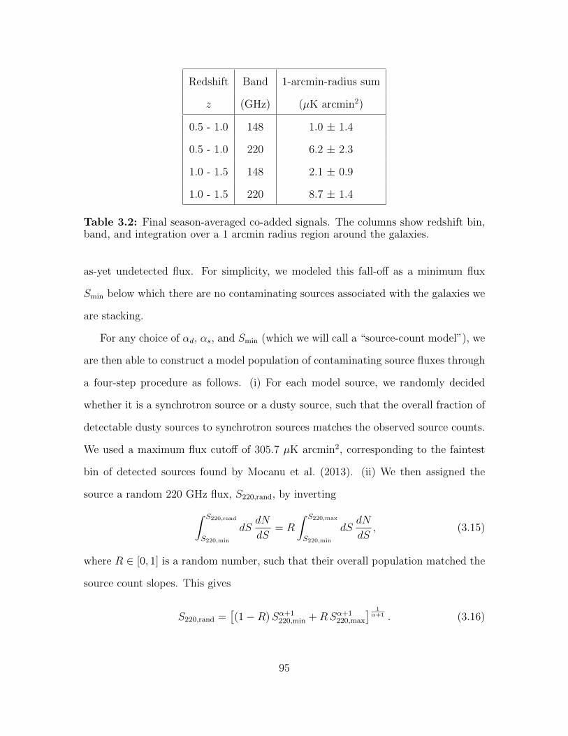
Redshift Band 1-arcmin-radius sum

z (GHz) (µK arcmin2)

0.5 - 1.0 148 1.0 ± 1.4

0.5 - 1.0 220 6.2 ± 2.3

1.0 - 1.5 148 2.1 ± 0.9

1.0 - 1.5 220 8.7 ± 1.4

Table 3.2: Final season-averaged co-added signals. The columns show redshift bin,band, and integration over a 1 arcmin radius region around the galaxies.

as-yet undetected flux. For simplicity, we modeled this fall-off as a minimum flux

Smin below which there are no contaminating sources associated with the galaxies we

are stacking.

For any choice of αd, αs, and Smin (which we will call a “source-count model”), we

are then able to construct a model population of contaminating source fluxes through

a four-step procedure as follows. (i) For each model source, we randomly decided

whether it is a synchrotron source or a dusty source, such that the overall fraction of

detectable dusty sources to synchrotron sources matches the observed source counts.

We used a maximum flux cutoff of 305.7 µK arcmin2, corresponding to the faintest

bin of detected sources found by Mocanu et al. (2013). (ii) We then assigned the

source a random 220 GHz flux, S220,rand, by inverting∫ S220,rand

S220,min

dSdN

dS= R

∫ S220,max

S220,min

dSdN

dS, (3.15)

where R ∈ [0, 1] is a random number, such that their overall population matched the

source count slopes. This gives

S220,rand =[(1−R)Sα+1

220,min +RSα+1220,max

] 1α+1 . (3.16)

95

(iii) To obtain a corresponding flux for the source at 148 GHz we used the α150220 spectral

index distributions from Mocanu et al. (2013), which we assume to have normalized

Gaussian shapes with the properties (center, σ) = (-0.55, 0.55) for synchrotron sources

and (3.2, 0.89) for dusty sources. We then randomly chose α150220 values that fit these

distributions and calculated the 148 GHz flux (following Mocanu et al., 2013) as

S148,rand =S220,rand

C1 × C2

, (3.17)

where C1 is the conversion factor between Jy and µK arcmin2 integrated over the

band filter curves, C2 is the relating factor (ν220/ν148)α150220 integrated over the band

filter curves, and we used units of µK arcmin2 for all S. (iv) Finally, we estimated

the completeness of our 220 GHz measurements and randomly discarded modeled

sources to match the estimated fraction of 220 GHz sources detected per flux. To do

the estimation, we assumed a cutoff Scut of 250 µK arcmin2, representing the 3σ limit

of our 220 GHz source measurements. We discarded galaxies with signals greater

than Scut or signals less than −Scut. We then determined the completeness fractions

for the modeled sources, and accounted for our measurement uncertainty, by adding

the 220 GHz random point distribution onto Scut in a cumulative manner using the

fraction of random point measurements below a given flux. This means Scut has a

50% completeness, while fainter fluxes are increasingly less complete and brighter

fluxes are increasingly more complete.

For each source-count model, we repeated the process 100,000 times, resulting in

a large catalog of contaminating fluxes in both bands. From these, we computed the

mean flux per contaminating source in each band, 〈S148,cont〉 and 〈S220,cont〉, which

represents the contamination we are measuring in our stacks. To account for varia-

tions in the input parameters, we computed model contamination signals for a wide

range of source-count models, with S220,max = 305.7µK arcmin2. We varied αs from

96

Model N z∫

∆T148(θ)dθ Y Etherm(±1σ) Etherm(±2σ) S/N

(µK arcmin2) (10−7 Mpc2) (1060 erg) (1060 erg) (Etherm/1σ)

Data only 1179 0.5− 1.0 1.0± 1.4 −0.8± 1.1 −2.8± 3.9 −2.8± 7.9 -0.72

3274 1.0− 1.5 2.1± 0.9 −1.9± 0.8 −7.0± 3.0 −7.0± 6.0 -2.33

χ2 (ACT only) 1179 0.5− 1.0 −1.6+1.8−1.9 1.2+1.4

−1.4 4.5+5.4−5.1 4.5+11.0

−10.7 0.85

3274 1.0− 1.5 −2.1+1.1−1.2 1.9+1.1

−1.0 7.0+4.0−3.7 7.0+8.4

−7.7 1.78

χ2 (With Planck) 227 0.5− 1.0 −2.0+2.0−2.1 1.5+1.6

−1.5 5.6+5.9−5.6 5.6+12.4

−11.6 0.97

529 1.0− 1.5 −2.1+1.3−1.4 1.9+1.3

−1.2 7.0+4.7−4.4 7.0+9.7

−9.4 1.50

Table 3.3: Our final tSZ measurements using various methods for removing contam-ination. The last three columns represent the best fit Etherm values with ±1σ valuesand ±2σ values and the Etherm signal-to-noise ratio (Etherm/1σ), respectively.

−2.26 to −1.90 in steps of 0.09 and we varied αd from −3.25 to −2.57 in steps of 0.17,

representing ranges of ±2σ in steps of σ. We let log10(Smin) vary from log10(0.01 µK

arcmin2) to log10(30 µK arcmin2) in steps of 0.2 in log-space.

For each source-count model, we computed best-fit tSZ values by varying our two

free parameters, tSZ signal (SSZ) and the fraction of our measured sources that are

contaminated (fcont). We varied the tSZ signal from -50 to 50 µK arcmin2 in steps

of 0.1 µK arcmin2, and we varied the fraction contaminated from -3 to 9 in steps of

0.01. For every combination of these parameters we computed a χ2 value,

χ2(fcont, SSZ) = B ×A−1 × BT , (3.18)

where B is the signal array,

B =

fcont × 〈S148,cont〉+ SSZ − S148

fcont × 〈S220,cont〉 − S220

, (3.19)

and A is the noise matrix containing the noise for each band plus the covariance terms

between each band,

A =

σ2148 σ148σ220

σ148σ220 σ2220

. (3.20)

97

Figure 3.7: Plot of the contaminant-corrected Etherm (see Equation (3.8)) for dif-ferent choices of αdust, αsync, and Smin. Points are located at the peak χ2 probabilityfor each model. Increasing size represents increasing (i.e. more positive) αs, andchanging color from red to black represents increasing αd. The light and dark grayregions represent the complete span of ±1σ and ±2σ, respectively, for all points.Black regions represent the most favorable models with peak χ2 probability. Thehorizontal solid black lines represent the best estimates for Egrav, and the horizontaldashed black lines represent the −1σ values for Egrav (see Equation (3.5)).

Here, S148, S220, σ148, and σ220 are our measured 1 arcmin radius values from Table

3.2. The σ values are computed using random point measurements, given by

σiσj =

∑Nrand

a=0 (Sai,rand − 〈Si,rand〉)× (Saj,rand − 〈Sj,rand〉)NrandNsource

, (3.21)

where i and j represent the bands, Sa,rand and Sb,rand represent the 1 arcmin radius

aperture values for the random points, Nrand = 294,176 is the number of random

points used, and Nsource is the number of galaxies used (1179 for low-z and 3274 for

high-z). We then converted the χ2 values to Gaussian probabilities P by taking

P (SSZ) =

∑fcont∈[0,1] exp[−χ2(fcont, SSZ)/2]∑fcont

∑SSZ

exp[−χ2(fcont, SSZ)/2]. (3.22)

98

where the lower sum over fcont runs from −3 to 9 and the lower sum over SSZ runs

from −50 to 50 µK arcmin2. Our approach was thus to marginalize over values of

fcont in the full physical range from 0 to 1, but normalize the overall probability by

the sum of fcont over a much larger range, including unphysical values. This excludes

models in which a good fit to the data can only be achieved by moving fcont outside

the range of physically possible values.

Equation (3.22) then gives us a function P (SSZ) for each combination of αd, αs,

and Smin. We can convert the corresponding SSZ value to the gas thermal energy,

Etherm, using Equation (3.8) and the average l2ang from Table 3.1. Note that a positive

detection of the tSZ effect is seen as a negative ∆T signal at 148 GHz, and it represents

a positive injection of thermal energy into the gas around the galaxy. Additionally,

we compute a corresponding range for Egrav using Equation (3.5) and values from

Table 3.1. The peak of each P (SSZ) curve is shown as the colored points in Figure

3.7, where αs (represented by point size) is increasing (i.e. becoming more positive)

downwards, and αd (represented by point color) is increasing upwards. The 1σ and

2σ contours are computed for each Smin by averaging P (SSZ) across αd and αs. The

resulting probability distribution depends only on Etherm and Smin, and 1σ and 2σ

are represented by the values P (SSZ) = 0.61 and 0.13, respectively (i.e. exp[−σ2/2]).

These contours are shown in Figure 3.7, along with the −1σ range for Egrav. Peak

probability values are chosen using P (SSZ) > 0.99, shown as the black regions in

Figure 3.7. From this figure we see that there is a ≈ 1σ tSZ detection for Smin & 3µK

arcmin2 at low-z. At high-z we see a ≈ 2σ tSZ detection for Smin & 5µK arcmin2.

Finally, we average the probability distribution across Smin to get a final distri-

bution as a function of only Etherm. The significance values of this curve are shown

in Table 3.3 under “ACT only.” We see a 0.9σ tSZ detection at low-z and a 1.8σ

detection at high-z.

99

3.8 Modeling and Removing Dusty Contamination With Planck

As indicated by Figure 3.6, we should be able to better constrain the contami-

nation due to undetected dusty sources by incorporating data at higher frequencies

than the ACT bands we are using to make our measurements. We therefore made

use of the 2015 public data release from the Planck mission, and focused on the high-

frequency bands at 217, 353, 545, and 857 GHz. These data, with a≈5 arcmin FWHM

beam (Planck Collaboration et al., 2015a), is too low-resolution to be useful in our

direct tSZ measurements, but can still provide useful information about our galaxies

at higher frequencies where the contaminant emission should be much brighter (see

the light blue and dark blue curves in Figure 3.6). By incorporating these Planck

measurements we should be able to better discriminate between contaminant models,

allowing us to better identify the true tSZ signal.

To utilize the Planck data, we followed the same process as in the previous section

by computing χ2 values for a number of modeled contaminants, but now we had

several extra terms in each computed χ2 relating to the Planck measurements. In

addition to the parameters used in the previous section, we also varied our models

over reasonable values for contaminating dust temperature and residual CMB primary

signal. Since there were now several more terms to fit, we could weight our final

probabilities by the best fitting χ2 values for each model. In order to stack our

galaxies in the Planck data, we first extended our contaminant source cut distance

from 4 to 10 arcmin due to the much lower resolution. This resulted in a significant

decrease in our number of galaxies, with 227 at low-z and 529 at high-z. In order to

filter out the primary CMB signal, we convolved each Planck map with a 7 arcmin

FWHM Gaussian and subtracted the resulting image from the original. We then

stacked the central pixels of each galaxy to get co-added values in each of the Planck

100

bands. In addition, we degraded the ACT 148 and 220 GHz maps to match the

Planck beam, applied the same 7 arcmin FWHM filtering, and stacked the central

pixels of galaxies in those images as well.

As was the case in Section 3.6, in all of these stacks there is an offset we needed

to correct for since we are purposely avoiding positive contaminations in the maps.

To do this we also made measurements at 54,962 random points on the sky that were

restricted to the same contaminating-source cuts as our galaxies. These measurements

allowed us to compute offset values needed to shift each band to a mean of 0, which

we applied to our final measurements.

Finally, we computed our measurement errors by using the random point mea-

surements (since the proper noise covariance matrix is not provided, i.e. Planck Col-

laboration et al., 2015b), corrected in two ways. First, because we account for the

residual CMB primary signal in the χ2 calculations, discussed below, we removed

the corresponding uncertainty term, taken to have a covariance of 7.85 µK as used in

Spacek et al. (2016). Second, there is an error introduced due to our offset corrections

because they are made from a large, but finite, number of points. We then get the

corrected error from

(σiσj)corr =

√σiσj − σ2

cov

Nsource

+σiσj

Nrandom

, (3.23)

where σiσj is given by Equation (3.21) with i and j representing the various bands

used, σcov = 7.85µK is the minimum CMB covariance discussed above, Nsource is the

number of sources used for the measurements (227 for low-z and 529 for high-z), and

Nrandom = 54,962 is the number of random points used. This represents both the

error due to detector noise in each band as well as the error due to contributions

from foregrounds on the sky. The majority of the variance at the highest frequen-

cies is correlated between the bands and likely due to contributions from Galactic

101

dust emission. However, unlike the primary CMB signal, the spectral shape of this

foreground is similar to that of the dusty sources we are trying to constrain, and it

cannot be removed by fitting it separately.

In the same manner as the previous section, we modeled ACT 148 and 220 GHz

contaminant source fluxes using a range of different source-count models (i.e. αd, αs,

and Smin), resulting again in 100,000 modeled contaminating source fluxes in each

ACT band, S148,cont and S220,cont. We also modeled what the contaminating signal

would be in the Planck bands and the ACT bands filtered to match Planck. For each

modeled contaminating source, if it was chosen to be a synchrotron source we simply

extrapolated the Planck-based fluxes as

Sν,sync = S148,cont ×(

ν

ν148

)α150220

× Cν × F, (3.24)

integrated over the relevant band filter curves, where α150220 is the same used in the

previous section, Cν is a frequency-dependent factor involved in the conversion from

Jy to µK arcmin2, and F = 0.021 is the factor required to preserve the signal within

a 1 arcmin radius aperture after applying the Planck filtering we used.

In order to accurately describe thermal dust emission across the Planck frequen-

cies, we adopted a modified blackbody with a free emissivity index, β, and dust tem-

perature, Tdust, often referred to as a gray-body (Planck Collaboration et al., 2015c).

This requires us to add another free parameter, the temperature of the contaminant

dust, Tdust. This slope of each dusty source as a function of frequency is then

d lnSνd ln ν

∣∣∣∣ν=185 GHz

= 3 + β − x185[1− exp(−x185)]−1, (3.25)

where x185 ≡ (185 GHz)×h/(kT ) = (185/416)(1 + z)/T20 and T20 is the dust temper-

ature in units of 20 K, and we use the slope of the blackbody function at ν = 185

GHz because it is halfway between our two ACT bands (148 and 220 GHz). This can

102

be related, in turn, to the power law index α150220 as

β + 3 = α150220 + x185[1− exp(−x185)]−1. (3.26)

This then gives

Sν,dust = S148,cont ×(

ν

ν148

)α150220+x185[1−exp(−x185)]−1

× exp[(ν148/416)(1 + z)/T20]− 1

exp[(ν/416)(1 + z)/T20]− 1× Cν × F,

(3.27)

integrated over the relevant band filter curves, where we vary Tdust from 20 to 50 K

in steps of 3 K.

With these expressions, we were able to compute χ2 values for each source-count

model accounting for the Planck measurements. This time, in addition to varying

fcont and SSZ, we also varied Tdust (as discussed above) and a parameter ∆, which

represents the offset due to the CMB primary signal, which we vary from -3 to 3 µK

in steps of 0.1 µK. Computing χ2 now involved the original ACT terms plus the new

Planck terms, and it followed the same process as in Equation (3.18),

χ2(fcont, SSZ, Tdust,∆) = B ×A−1 × BT , (3.28)

where B is the signal array and A is the noise matrix containing the noise for each

band plus the covariance terms between each band. We denote each element of the

signal array Bi, where i runs over the two ACT bands (i.e. 148 and 220 GHz) and

then every Planck-filtered band (i.e. the Planck bands at 857, 545, 353, and 217

GHz, plus the ACT bands at 220 and 148 GHz filtered to match the Planck images),

such that B1 = fcont × 〈S148,cont〉 + SSZ − S148, B2 = fcont × 〈S220,cont〉 − S220, and

B3−8 = fcont × 〈S3−8,cont〉+ ∆− S3−8. As before, Si represents the final values of our

galaxy stacks for each band. We similarly define the elements of the noise matrix as

Aij = σiσj, where i and j run over all of the bands and σiσj is given by Equation

(3.23).

103

Figure 3.8: Plot of the contaminant-corrected Etherm (see Equation (3.8)) for differ-ent choices of αdust, αsync, and Smin, incorporating the Planck bands. The light anddark gray regions represent the complete span of ±1σ and ±2σ, respectively, for allpoints, and the black regions represent the peak of the χ2 probability distribution,i.e. the most favorable models. The horizontal solid black lines represent the bestestimates for Egrav, and the horizontal dashed black lines represent the −1σ valuesfor Egrav (see Equation (3.5)).

As in the previous section, we then converted the χ2 values to Gaussian probabil-

ities by taking

P (SSZ) =∑

fcont∈[0,1],Tdust,∆

exp[−χ2(fcont, SSZ, Tdust,∆)/2]∑all exp[−χ2/2]

, (3.29)

where the whole function is normalized to a total of 1, and each final SZ value contains

the sum over the corresponding Tdust, ∆, and fractions from 0 to 1. Since in this case

there are eight terms contributing to χ2 and four fit parameters, this leaves us with

four degrees of freedom. Thus the minimum χ2 was not 0 in every case as it was

above with just 2 measurements and 2 fit parameters, and so for each model we scale

the final probabilities by exp(−χ2min/2), where χ2

min is the minimum χ2 value for that

model.

104

Study N Type z (mean) Mass (M) tSZ Y (10−7 Mpc2)

Spacek et al. (2016) 3394 SPT 0.5− 1.0 (0.72) 1.51× 1011 2.3+0.9−0.7

Spacek et al. (2016) 924 SPT 1.0− 1.5 (1.17) 1.78× 1011 1.9+2.4−2.0

Spacek et al. (2016) 937 SPT+Planck 0.5− 1.0 (0.72) 1.51× 1011 2.2+0.9−0.7

Spacek et al. (2016) 240 SPT+Planck 1.0− 1.5 (1.17) 1.78× 1011 1.7+2.2−1.8

Current 1179 ACT 0.5− 1.0 (0.83) 7.81× 1011 1.2+1.4−1.4

Current 3274 ACT 1.0− 1.5 (1.20) 10.1× 1011 1.9+1.1−1.0

Current 227 ACT+Planck 0.5− 1.0 (0.83) 6.93× 1011 1.5+1.6−1.5

Current 529 ACT+Planck 1.0− 1.5 (1.21) 9.68× 1011 1.9+1.3−1.2

Table 3.4: A comparison between Spacek et al. (2016) and the current work. Y isthe angularly integrated Compton-y parameter given by Equation (3.30). Mass refersto stellar mass.

This again gave us a function P (SSZ) for each combination of αd, αs, and Smin,

which we can convert to an energy Etherm. The 1σ and 2σ contours are created for

each Smin by averaging P (SSZ) across αd and αs and then dividing the final result

by the single maximum value. 1σ and 2σ are again represented by the values 0.61

and 0.13, respectively, with peak probability values represented by P (SSZ) > 0.99.

These contours are shown in Figure 3.8, along with the −1σ range for Egrav. From

this figure we can see that, for low-z, including Planck has slightly increased the

estimated tSZ effect, though it now favors higher Smin values. The high-z result has

not changed much besides an increased uncertainty due to fewer galaxies. For both

redshift bins, the σ values have increased due to the large decrease in the number of

stacked galaxies because of Planck’s much larger beam.

Finally, we average the probability distribution across Smin, divided by the max-

imum value again, and get a final distribution as a function of only Etherm. The

significance (σ) values of this curve are shown in the “With Planck” part of Ta-

ble 3.3. At low-z, the significance of our tSZ detection has increased from 0.9σ to

105

1.0σ, while at high-z the tSZ detection significance decreases from 1.8σ to 1.6σ. It is

clear that the gain in sensitivity with Planck has been limited by the decrease in the

number of galaxies in each redshift bin due to the much larger beam size of Planck

compared to the ACT. To clearly show this, we followed the methods of Section 3.7

(i.e. only ACT data were used), using this limited galaxy sample. The result is a

0.1σ tSZ detection at low-z and a 0.5σ tSZ detection at high-z. It is apparent, then,

that adding the Planck data helps immensely with constraining the tSZ signal when

the same number of galaxies are used, but since we have to limit our galaxy sample

size so much to avoid contaminants in the Planck beam, the loss of accuracy due to

fewer measurements just about offsets the gain in accuracy given by the added Planck

data.

Alternatively, we can also characterize the total tSZ signal for our co-adds with

the angularly integrated Compton-y parameter, Y . While we cannot directly com-

pare peak Compton-y values with past measurements, as these are beam-dependent

quantities, we can compare the angularly integrated Y values between our results and

past experiments. Using Equation (3.7) at 148 GHz, this is

Y ≡ l2ang

∫y(θ)dθ

= −3.2× 10−8 Mpc2

(lang

Gpc

)2 ∫ ∆T148(θ)dθ

µK arcmin2 ,

(3.30)

such that Y = 2.7× 10−8 Mpc2E60, where E60 is Etherm in units of 1060 erg. We can

use this to compare the results in this paper with the similar work in Spacek et al.

(2016), with a detailed comparison shown in Table 3.4. Comparing the two results,

we see a decrease in Y at low-z in this work compared to Spacek et al. (2016), and

similar Y values at high-z, but we also see a significant increase in the average galaxy

mass. This is contrary to the expected trend of higher Y with higher mass seen in

106

Figure 3.9: Plot of Y vs. stellar mass for Spacek et al. (2016) (black circles), thecurrent work (red circles), Planck Collaboration et al. (2013) (blue squares), Grecoet al. (2015) (orange diamonds), and Ruan et al. (2015) (light blue triangles). UsingEquations (3.5), (3.6), and (3.30), we can use our simple models to make estimates of

Y vs. stellar mass. These model estimates are shown for gravitational heating only(black line for z = 0.8, blue line for z = 1.2) and gravitational plus AGN feedbackheating (red line for z = 0.8, orange line for z = 1.2), with ±1σ errorbars.

previous work (e.g. Planck Collaboration et al., 2013; Greco et al., 2015; Ruan et al.,

2015).

We can compare with this previous work by defining Y ≡ Yl2ang×E−2/3×

(lang

500 Mpc

)2

,

where E(z) is the Hubble parameter, and this is shown in Figure 3.9. The circles

represent Spacek et al. (2016) (black) and this work (red), both using measurements

of massive quiescent elliptical galaxies with average redshifts greater than 0.7 for

the lower-mass values of either color and 1.1 for the higher-mass values of either

color. The blue squares represent Planck Collaboration et al. (2013) measurements

107

of locally brightest galaxies, with redshifts less than ≈0.3. The orange diamonds

represent Greco et al. (2015) measurements of locally brightest galaxies, with redshifts

less than ≈0.3. The light blue triangles represent Ruan et al. (2015) measurements

of locally brightest galaxies, with median redshifts of ≈0.5 and redshifts less than

≈0.8. Looking at this figure, we see that the results of Spacek et al. (2016) are

roughly consistent with the previous tSZ measurements, while the results of this

work are over ≈2 orders of magnitude smaller than previous tSZ measurements at

the same mass. We note that the measurements of locally brightest galaxies from

Planck Collaboration et al. (2013), Ruan et al. (2015), and Greco et al. (2015) are

of significantly lower redshifts than our galaxies, with the highest overall redshift

being no more than ≈0.8 from Ruan et al. (2015) while our average redshifts range

from 0.7 to 1.2. In addition, our selection criteria involve choosing quiescent elliptical

galaxies and removing any galaxies in or around all detectable clusters, while the

low-redshift locally brightest galaxies of the previous studies are more likely to be

found in the centers of massive galaxy groups and clusters. Redshift alone cannot

account for the ≈2 orders of magnitude difference in measurements, as is made clear

by the black and red lines representing our models at z = 0.8 (without and with

AGN feedback, respectively) and the blue and orange lines representing our models

at z = 1.2 (without and with AGN feedback, respectively). However, the differences

in redshift combined with the different galaxy selection methods suggest that the

galaxies used in this paper could be from fundamentally different populations and

environments.

With Equations (3.5) and (3.6) and the redshifts and masses from Table 3.1, we

can also investigate theoretical thermal energies of the gas around elliptical galaxies

due to both gravity and AGN feedback. Without Planck, we estimate the gravita-

tional heating energy to be Etherm,grav = 17.0+17.0−9.1 × 1060 erg for our low-z sample

108

and Etherm,grav = 16.7+16.7−9.0 × 1060 erg for our high-z sample. We therefore measure

excess non-gravitational energies of Etherm,feed,dat = −12.5+17.7−10.6 × 1060 erg for low-z

and Etherm,feed,dat = −9.7+17.1−9.8 × 1060 erg for high-z, both of these values consistent

with zero detection. For completeness, we can plug these into the theoretical AGN

feedback energy equation and solving for εk, we get feedback efficiencies of −4.8+6.8−4.1%

for low-z and −3.8+6.7−3.9% for high-z.

With Planck, we estimate the gravitational heating energy to be Etherm,grav =

15.1+15.1−8.1 × 1060 erg for our low-z sample and Etherm,grav = 15.9+15.9

−8.5 × 1060 erg for our

high-z sample. We therefore measure excess non-gravitational energies of Etherm,feed,dat

= −9.5+16.1−10.0 × 1060 erg for low-z, and Etherm,feed,dat = −8.9+16.5

−9.7 × 1060 erg for high-z,

both consistent with 0. Plugging these into the theoretical AGN feedback energy

equation and solving for εk, we get feedback efficiencies of −4.1+7.0−4.4% for low-z and

−3.7+6.8−4.0% for high-z. These values are very uncertain and consistent with a detected

AGN feedback signal of 0. They also do not rule out the suggested and measured

≈5% (e.g. Scannapieco et al., 2005; Ruan et al., 2015; Spacek et al., 2016). We also

note that the feedback efficiencies stated in Spacek et al. (2016) are mistakenly off by

a factor of 5, and they should be 7.3+6.6−7.8% for low-z and 6.6+17.3

−15.3% for high-z.

3.9 Discussion

In this paper we have performed a stacking analysis of the tSZ signal around

4453 massive elliptical galaxies that are promising candidates for containing relic

heating due to past episodes of AGN feedback. We split our selected galaxies into

two redshifts bins, with 1179 galaxies in our “low-z” bin (0.5 ≤ z ≤ 1.0) and 3274

galaxies in our “high-z” bin (1.0 ≤ z ≤ 1.5). Our initial stacks were dominated

by considerable contaminating emission which was much stronger at 220 GHz than

at 148 GHz. Since dusty contaminant emission emits at both 148 and 220 GHz,

109

as suggested by Figure 3.6, the large signals at 220 GHz, where the tSZ effect is

expected to be negligible, indicate a corresponding large contaminant signal at 148

GHz, where the tSZ effect causes a decrement. We therefore performed an analysis

of the contaminating signal by modeling potential undetected sources and running a

χ2 probability test on the models. This revealed the underlying tSZ signal, with a

0.9σ significance at low-z and a 1.8σ significance at high-z. Finally, in order to better

constrain the stacked contaminating signal, we incorporated high-frequency Planck

measurements of a subset of 227 low-z galaxies and 529 high-z galaxies. These results

indicated tSZ detections with a 1.0σ significance at low-z and a 1.6σ significance at

high-z. The values for each of these analyses are given in Table 3.3.

The work done here is complementary to the work done in Spacek et al. (2016),

which stacked 4318 galaxies in a southern patch of sky using SPT data, while we

stacked 4453 galaxies in the Stripe-82 equatorial band using ACT data. Both analyses

used similar galaxy selection criteria, though that of Spacek et al. (2016) favored

lower-mass, 0.5 ≤ z ≤ 1.0 “low-z” galaxies while our selection favored 1.0 ≤ z ≤ 1.5

“high-z” galaxies with higher stellar masses. Their most significant low-z and high-z

tSZ detections were at 3.6σ and 0.9σ levels, respectively, while ours were at 1.0σ and

1.8σ, respectively. A detailed comparison between the two studies can be seen in

Table 3.4, where we see similar tSZ Y measurements in this work, although we use

galaxies with higher masses. A plot comparing these results, as well as results from

other previous galaxy tSZ measurements from Planck Collaboration et al. (2013),

Greco et al. (2015), and Ruan et al. (2015), is shown in Figure 3.9. These last three

results appear to be significantly higher than the results of this paper. This may

be due to several factors, including inherent differences in the measurements due

to different galaxy populations. The previous studies focus on lower-redshift locally

brightest galaxies, while this work looks at quiescent elliptical galaxies at significantly

110

higher redshifts. We also perform extensive cuts to avoid clusters and dusty galaxies.

There is the additional possibility that we are not completely accounting for and

removing the contamination signal in this work despite our best efforts, though this

seems unlikely to be the main reason for the discrepancy. Also shown in Figure 3.9

are lines representing our simple gravitational and AGN feedback heating models

given by Equations (3.5) and (3.6). These simple models indicate that the types of

galaxies and redshifts that we are looking at are expected to produce significantly

lower tSZ measurements. The measurements presented here are also unique, with

a review of the literature revealing no other similar measurements of the tSZ signal

around such massive, high-redshift, quiescent elliptical galaxies. It therefore may not

be completely appropriate to make direct comparisons between these measurements

and measurements of less massive, lower-redshift locally brightest galaxies. While

Spacek et al. (2016) estimate AGN feedback efficiencies of around ≈7%, close to

the suggested 5% (e.g. Scannapieco et al., 2005; Ruan et al., 2015), this work sees

an AGN feedback heating signal consistent with 0, with efficiencies of −4.1+7.0−4.4%

for low-z and −3.7+6.8−4.0% for high-z. It is important to note, however, that we use

simple, general models of gravitation and AGN feedback in this paper to estimate

the corresponding energies, and that specific, detailed galaxy simulations are needed

to draw more precise conclusions from these measurements.

tSZ measurements of galaxies and AGNs are likely to improve significantly in the

near future. More data and an additional band at 277 GHz will be released from ACT

observations (Dunner et al., 2013), while an upcoming full survey release of SPT data

will include a 2500 deg2 field using bands at 95, 150, and 220 GHz (Schaffer et al.,

2011). These much larger fields with more bands will allow for a much larger set of

galaxies to be co-added at more frequencies, vastly improving the signal-to-noise of the

measurements and allowing for further constraints on contaminating signals. Separat-

111

ing out such contaminants will also become more effective with future surveys such as

the upgraded ACT telescope (Advanced ACTPol) and the proposed Cerro Chajnan-

tor Atacama Telescope (CCAT).15 Another approach to constraining AGN feedback

is through deep measurements of smaller samples of galaxies, identified as the most

interesting, using large radio telescopes. The Goddard IRAM Superconducting Two

Millimeter Camera (GISMO) and the New IRAM KIDs Array (NIKA) are powerful

new instruments mounted on the Institute de Radioastronome Millimetrique (IRAM)

30 m telescope16 that may prove useful for this purpose. Also promising is the National

Radio Astronomy Observatories (NRAO) Green Bank Telescope (GBT), whose Con-

tinuum Backend operates at lower frequencies where the tSZ signal is roughly three

times larger. Finally, although tSZ observations reveal the total thermal heating

around galaxies, they must be complimented by theoretical models and simulations

in order to best distinguish between heating due to gravitation, AGN feedback, and

other effects. Observations can therefore be combined with tSZ simulations of the

same types of objects with the same average parameters (e.g. mass, redshift, age)

to produce weighted stacks that are adapted to be as sensitive as possible to the

differences between AGN feedback models. The tSZ effect provides a promising tool

for future measurements to improve our understanding of AGN feedback and galaxy

evolution.

15http://www.ccatobservatory.org/

16http://www.iram-institute.org/EN/30-meter-telescope.php

112

Chapter 4

USING REAL AND SIMULATED MEASUREMENTS OF THE THERMAL

SUNYAEV-ZEL’DOVICH EFFECT TO CHARACTERIZE AND CONSTRAIN

MODELS OF AGN FEEDBACK

4.1 Introduction

Galaxies are some of the most common and prominent objects in the Universe.

As important as they are, the processes governing their formation and evolution are

surprisingly uncertain. Although simple early models favored hierarchical growth in

which progressively larger galaxies are expected to form stars at later times (e.g. Rees

& Ostriker, 1977; White & Frenk, 1991), an increasing amount of observational ev-

idence reveals galaxy evolution to be more complex (e.g. Cowie et al., 1996). Since

z ≈ 2 the typical mass of star-forming galaxies has decreased by a factor of ≈10

or more (Drory & Alvarez, 2008). The same goes for active galactic nucleus (AGN)

evolution, where the typical luminosity of AGNs is observed to have decreased by as

much as a factor of ≈1000 since z ≈ 2 (Hopkins et al., 2007). This observed downsiz-

ing trend of both galaxies and AGNs, combined with other well-known relationships

between supermassive black holes and their host galaxies like the MBH–σ? relation

(e.g. Shankar et al., 2016), points to a mechanism affecting both the small scale of

the supermassive black hole (. 1 ly) and the large scale of the galaxy (& 100 kly).

One such mechanism that has been proposed to resolve many of the problems

mentioned above is the AGN phase of the supermassive black hole (e.g. Sijacki et al.,

2007). AGNs are energetic enough to drive out enormous, powerful radio jets, as well

as extremely luminous radiative winds, causing energetic outflows through the host

113

galaxy. This feedback has the potential to blow out and heat up cool gas within and

around the galaxy, preventing both further star formation in the galaxy and further

accretion onto the supermassive black hole. Incorporating AGN feedback into numer-

ical galaxy evolution models has been shown to be very effective in reproducing the

observed downsizing (e.g. Scannapieco & Oh, 2004; Sijacki et al., 2007; Hirschmann

et al., 2012; Lapi et al., 2014; Kaviraj et al., 2016). However, the specific details of

AGN feedback remain uncertain because precise details are very difficult to measure

(e.g. Fabian, 2012).

One of the most promising methods for directly measuring the impact of AGN

feedback on galaxies and clusters is by looking at anisotropies in the cosmic microwave

background (CMB) photons passing through hot, ionized gas, known as the Sunyaev-

Zel’dovich (SZ) effect (Sunyaev & Zeldovich, 1972). If the gas is moving with a bulk

velocity, there will be frequency-independent fluctuations in the CMB temperature

known as the kinematic SZ (kSZ) effect, which can be used to detect the profile

of ionized gas within dark matter halos, providing information on where hot gas is

located around galaxies. This method is becoming increasingly promising, with some

of the first detections of the kSZ effect in galaxy clusters made recently by stacking

CMB observations with Planck (Planck Collaboration et al., 2016), the South Pole

Telescope (SPT) (Soergel et al., 2016), and the Atacama Cosmology Telescope (ACT)

(Schaan et al., 2016).

Additionally, if the gas is sufficiently heated, there will be redshift-independent

fluctuations in the CMB temperature known as the thermal SZ (tSZ) effect, which can

be integrated over a region of the sky to give a direct measurement of the gas thermal

energy (e.g. Scannapieco et al., 2008). Measurements of the tSZ effect have been very

useful in detecting massive galaxy clusters (e.g. Reichardt et al., 2013). Simulations

114

have also shown that the tSZ effect can be effective in distinguishing between models

of AGN feedback (e.g. Chatterjee et al., 2008; Scannapieco et al., 2008).

Significant observational work has already been done to try and measure the tSZ

effect. For example, Chatterjee et al. (2010) used data from WMAP and SDSS around

both quasars and galaxies to find a tentative tSZ signal suggesting AGN feedback;

Hand et al. (2011) used data from SDSS and ACT to find a significant tSZ signal

around galaxies; Gralla et al. (2014) used ACT to find a significant tSZ signal around

AGNs; Greco et al. (2015) used SDSS and Planck to find a significant tSZ signal

round galaxies; Ruan et al. (2015) used SDSS and Planck to find significant tSZ

signals around both quasars and galaxies; Crichton et al. (2016) used SDSS and ACT

to find a significant tSZ signal around quasars; and Hojjati et al. (2016) used data

from Planck and RCSLenS to find a tSZ signal suggestive of AGN feedback.

Additionally, recent measurements have been made around quiescent, moderate

redshift elliptical galaxies (Spacek et al., 2016, 2017), where a signal due to AGN

feedback is expected (e.g. Scannapieco et al., 2008). The signal is very faint, though,

so measurements from a large number of galaxies must be stacked. Spacek et al.

(2016) performed this type of stacking analysis using the VISTA Hemisphere Survey

(VHS) and Blanco Cosmology Survey (BCS) along with the 2011 SPT data release,

finding a signal hinting at non-gravitational heating based on simple energy models.

Spacek et al. (2017) used the Sloan Digital Sky Survey (SDSS) and Wide-Field In-

frared Survey Explorer (WISE) along with the 2008/2009 ACT data, finding a signal

consistent with gravitational-only heating based on the same simple energy models.

These SPT and ACT results are shown in Figure 4.1 (black and red circles, respec-

tively), along with the simple model predictions and some previous studies. Note the

large discrepancy between the higher-mass ACT results and previous measurements

using Planck data, which is likely due to the differences in redshift, environment, and

115

Figure 4.1: Plot of normalized angularly-integrated tSZ signal vs. stellar massfor Spacek et al. (2016) (black circles), Spacek et al. (2017) (red circles), PlanckCollaboration et al. (2013) (blue squares), Greco et al. (2015) (orange diamonds),and Ruan et al. (2015) (light blue triangles). Solid lines are estimates using simplemodels from (Spacek et al., 2016), shown for gravitational heating only (black linefor z = 0.8, blue line for z = 1.2) and gravitational plus AGN feedback heating (redline for z = 0.8, orange line for z = 1.2), with ±1σ errorbars.

overall galaxy population being studied in these various papers. This highlights the

need to look at a diverse range of galaxies in order to understand the complete picture

of thermal heating.

Directly measuring the energy and distribution of hot gas around galaxies can only

reveal so much about the specific physical mechanisms resulting in the observations.

In order to place constraints on AGN feedback and other non-gravitational heat-

ing processes, it is necessary that observational work be complimented by accurate,

detailed simulations. There is a rich history of complementing tSZ measurements

and AGN feedback with simulations. For example, both Scannapieco et al. (2008)

116

and Chatterjee et al. (2008) used large-scale cosmological simulations to give details

about the possibilities of measuring AGN feedback with the tSZ effect, Cen & Sa-

farzadeh (2015b) used simulations to investigate the feedback energies from quasars

and implications for tSZ measurements, Hojjati et al. (2015) used large-scale cos-

mological simulations to estimate AGN feedback effects on cross-correlation signals

between gravitational lensing and tSZ measurements, and Dolag et al. (2016) used

large-scale simulations to study the impact of structure formation and evolution with

AGN feedback on tSZ measurements.

In this work, we utilize the large-scale cosmological simulations Horizon-AGN and

Horizon-noAGN, which are simulations with and without AGN feedback, respectively

(Dubois et al., 2012, 2014; Kaviraj et al., 2015, 2016), to compliment the work done

in Spacek et al. (2016, 2017). We will investigate looking at a similar population of

moderate redshift, quiescent elliptical galaxies and simulate their tSZ measurements.

We will then use their measurement distribution and stacking statistics to give insight

into the previous observational results. These Horizon simulations have a comoving

volume of 100 Mpc/h, 10243 dark matter particles, and a minimum cell size of 1

physical kpc, which allow for a large enough population of the generally uncommon

galaxies we are interested in.

The structure of this paper is as follows: in Section 4.2, we discuss the tSZ effect

and various models of AGN feedback. In Section 4.3, we discuss the Horizon-AGN

simulation. In Section 4.4, we discuss how we select and measure the tSZ effect around

galaxies. In Section 4.5, we give the parameters and measurements of our selected

galaxies. In Section 4.6, we discuss implications for our results in regard to Spacek

et al. (2016, 2017) and tSZ measurements of AGN feedback in general.

Throughout this work, we use a Λ Cold Dark Matter cosmological model with

parameters (from Planck Collaboration et al., 2015d), h = 0.68, Ω0 = 0.31, ΩΛ =

117

0.69, and Ωb = 0.049, where h is the Hubble constant in units of 100 km s−1 Mpc−1,

and Ω0, ΩΛ, and Ωb are the total matter, vacuum, and baryonic densities, respectively,

in units of the critical density.

4.2 The tSZ Effect

When CMB photons pass through hot, ionized gas along our line of sight, inverse

Compton scattering between the photons and electrons causes the photons to gain

energy. The resulting shift in the CMB spectrum has a distinctive frequency depen-

dence, with a weaker signal below, and a stronger signal above, 217.6 GHz. The

nonrelativistic change in the CMB temperature ∆T as a function of frequency ν due

to the tSZ effect is

∆T

TCMB

= y

(xex + 1

ex − 1− 4

). (4.1)

Here, TCMB = 2.725 K is the CMB temperature, x is a dimensionless frequency given

by x ≡ hνkTCMB

= ν56.81 GHz

, h is the Planck constant, k is the Boltzmann constant, and

the dimensionless Compton-y parameter is defined as

y ≡∫dl σT

nek (Te − TCMB)

mec2, (4.2)

where σT is the Thomson cross section, me is the electron mass, c is the speed of light,

ne is the electron number density, Te is the electron temperature, and the integral is

performed over the line-of-sight distance l.

When observing the tSZ effect on the sky, a useful quantity is the angularly

integrated Compton-y parameter, Y , given by

Y ≡ l2ang

∫y(θ)dθ, (4.3)

where lang is the angular diameter distance. For the SPT 150 GHz parameters from

Spacek et al. (2016), this is YSPT = 2.7×10−8 Mpc2E60, where E60 is the total line-of-

sight gas thermal energy Etherm in units of 1060 erg. For the ACT 148 GHz parameters

118

from Spacek et al. (2017), this is YACT = 2.9× 10−8 Mpc2E60. The values are slightly

different due to the slightly different frequency sensitivities and beam profiles of the

two telescopes. Y can additionally be scaled and written as (i.e. Planck Collaboration

et al., 2013)

Y ≡ Y

l2ang

× E−2/3 ×(

lang

500 Mpc

)2

, (4.4)

where E(z) ≡√

Ω0(1 + z)3 + ΩΛ is the Hubble parameter.

Spacek et al. (2016, 2017) use simple models of heating due to gravitation and

AGN feedback to compare with the above observational equations. For gravity, they

assume that as gas collapses and virializes along with an encompassing spherical halo

of dark matter, it is shock-heated to a virial temperature Tvir. For isothermal gas,

this gives a total thermal energy of

Etherm,gravity =3kTvir

2

Ωb

Ω0

M

µmp

= 1.5× 1060 ergM5/313 (1 + z), (4.5)

where mp is the proton mass, µ = 0.62 is the average particle mass in units of mp,

and M13 is the mass of the halo in units of 1013M. Using the relation between halo

mass and stellar mass described in Spacek et al. (2016, 2017), Mstellar = 2.8+2.4−1.4 ×

1010MM5/313 (1 + z)5/2, this gives

Etherm,gravity = 5.4+5.4−2.9 × 1060 erg

Mstellar

1011M(1 + z)−3/2. (4.6)

This is the total thermal energy expected around a galaxy of stellar mass Mstellar

ignoring both radiative cooling, which will decrease Etherm, and AGN feedback, which

will increase it.

For AGN feedback, they use the simple model described in Scannapieco & Oh

(2004), where the black hole emits energy at the Eddington luminosity, LEdd = 1.26×

1038(MBH/M)erg s−1 (e.g. Shankar et al., 2013), for a time 0.035 tdynamical, with

tdynamical ≡ Rvir/vc = 2.6 Gyr (1 + z)−3/2, and the gas is heated by a fraction εk of the

119

total bolometric luminosity of the AGN. This gives

Etherm,feedback = 4.1× 1060 erg εk,0.05Mstellar

1011M(1 + z)−3/2, (4.7)

where εk,0.05 ≡ εk/0.05 represents a typical efficiency factor of 5%.

4.3 The Horizon-AGN Simulation

The Horizon-AGN simulation is a cosmological hydrodynamical simulation that

uses the adaptive mesh refinement Eulerian hydrodynamics code RAMSES (Teyssier,

2002). The simulation is described in more detail in Dubois et al. (2012, 2014)

and Kaviraj et al. (2015, 2016), and here we will just restate some of the most

relevant information. The simulation box is 100/h Mpc comoving on each side, with

10243 dark matter particles at a resolution of 8 × 107M. The simulation grid is

refined throughout the simulation, with a minimum cell size of 1 physical kpc. Gas

cools through emission by H, He, and metals. Stars are created when the density of

hydrogen gas reaches 0.1 cm−3, and star particles have a resolution of ≈ 2× 106M.

Black holes are seeded at 105M when the gas and stellar densities and stellar

velocity dispersion are high, with a maximum accretion rate at the Eddington limit

and a radiative efficiency of 0.1. When the accretion rate is high (> 0.01LEdd), a

quasar-like feedback mode is assumed with 1.5% of the accretion energy injected as

thermal energy in the surrounding gas. When the accretion rate is low (< 0.01LEdd),

a radio feedback mode is assumed with bipolar jets at 10% efficiency. Feedback

parameters are chosen to match the MBH −M? and MBH − σ? relations observed at

z = 0. Black holes are said to merge when they are closer than 4 kpc and slower than

their mutual escape velocity.

120

Figure 4.2: Number of galaxies per redshift bin for the initial population, afterremoving active black holes, and then after matching both the SpSPT and SpACTmass distributions. On the left is the Y-AGN simulation and on the right is theN-AGN simulation.

4.4 Data

We use the Horizon-AGN (abbreviated here as “Y-AGN”) and Horizon-noAGN

(abbreviated here as “N-AGN”) simulations for our simulated galaxy data, and make

comparisons with observational measurements from Spacek et al. (2016) (abbreviated

here as “SpSPT”) and Spacek et al. (2017) (abbreviated here as “SpACT”). In order

to obtain as robust of a galaxy sample as possible, we collect data from the full

available spread of redshift outputs: 0.52, 0.56, 0.59, 0.63, 0.67, 0.72, 0.76, 0.81, 0.86,

0.91, 0.97, 1.03, 1.09, 1.16, 1.23, 1.31, 1.40, and 1.49. We initially find all galaxies

in the simulations with at least 250 star particles at each redshift. We then extract

various parameters for each galaxy (stellar mass, age, star formation rate, and active

black hole flag in the Y-AGN case) and corresponding dark matter halo (total mass,

gas mass, stellar mass, black hole mass, and dark matter mass) in both Y-AGN and

N-AGN. The active black hole flag says that a black hole is active if its mass is greater

than 106M and its luminosity is greater than 0.01LEdd. The stellar mass is taken

121

within a radius R200, defined as the radius enclosing an overdensity of 200 times the

critical density, given by

M(< R200)43πR3

200

= 200ρc(z), (4.8)

where M(< R200) is the mass enclosed within R200, and ρc(z) = 3H2(z)/(8πG). We

then perform a cut on the galaxies corresponding to the selection criteria in SpSPT

and SpACT, requiring Mstellar ≥ 1011M, Age ≥ 1 Gyr, and a non-active black hole

in the Y-AGN case. In addition, to prevent spurious measurements from galaxies

near the edge of the simulation box, we require dark matter halos to be at least 10

R200 away from any edge. The simulation is periodic and these galaxies could be

correctly measured by including the other side of the box, but since only a handful

of galaxies are excluded using this constraint we decide to use this cut for simplicity.

The number of galaxies left after the initial parameter cuts and the active black hole

cut at each redshift bin is shown in Figure 4.2.

We will note that we see a steady increase in the fraction of galaxies that are

flagged as active as we increase in redshift, generally < 20% for 0.5 < z < 1.0

(15% mean) and > 20% for 1.0 < z < 1.5 (25% mean). This makes sense, since

z ≈ 2 represents the peak of AGN activity, and it should decrease for lower z. The

0.7 < z < 0.8 bin is the one outlier, with 42% of the galaxies flagged as active. This is

due solely to the z = 0.76 data, which flagged 72% of its galaxies as active, much more

than it should have. This does not have any major effect on our results, though, since

the lower redshift galaxies are plentiful and the final SpSPT and SpACT matching

cuts are limited by the number of higher redshift galaxies.

For each galaxy, we use the electron pressure to compute Compton-y values (Equa-

tion 4.2) and then project these values into the x, y, and z directions. We then select

a square region around each galaxy and simulate measurements corresponding to the

beam and pixel sizes in both SpSPT and SpACT. For SpSPT, we use regions that are

122

Figure 4.3: Mass selection comparisons.

8.25 × 8.25 arcmin, 33 × 33 pixels, convolved with a 1.15 arcmin FWHM Gaussian

(corresponding to the 150 GHz SPT beam). For SpACT, we use regions that are

8.36 × 8.36 arcmin, 17 × 17 pixels, convolved with a 1.44 arcmin FWHM Gaussian

(corresponding to the 148 GHz ACT beam). This results in a selection of galaxies for

both Y-AGN and N-AGN at 0.5 < z < 1.5 with tSZ measurements in the x, y, and

z projections matching both SpSPT and SpACT. For simplicity, we will use only the

x projections from now on, with the y and z results being very similar.

4.5 Measurements

In order to compare the simulated galaxies with the observational galaxies, we ran-

domly build a population of simulated galaxies until their mass distribution matches

the histogram distributions in SpSPT and SpACT. The matched distribution is scaled

by whichever bin has the lowest fraction of Horizon galaxies compared to that bin

for SpSPT or SpACT. An issue arises since the SpACT mass distribution is skewed

to higher masses while the overall Horizon distributions favor lower masses. This

makes it difficult to match the SpACT distribution at the highest masses, so instead

123

Figure 4.4: Redshift and age selection comparisons. The left plots are comparisonswith SPT and the right plots are comparisons with ACT.

we choose some mass limit for each Horizon subset where we just keep all Horizon

galaxies above that mass. This is especially clear for the Y-AGN z = 1.0 − 1.5 line

in the right plot of Figure 4.3, where we only match the SpACT distribution up to

≈ 1012M and keep every galaxy above that. The original SpSPT and SpACT distri-

butions for mass along with the matched Horizon distributions are shown in Figure

4.3. The resulting SpSPT, SpACT, and Horizon distributions for redshift and age are

shown in Figure 4.4, the final number of Horizon galaxies at each redshift bin after

124

Final bin: Number N(SpSPT/SpACT)

SPT low-z Y-AGN: 5345 937

SPT low-z N-AGN: 19249 937

SPT high-z Y-AGN: 2293 240

SPT high-z N-AGN: 12004 240

ACT low-z Y-AGN: 1154 227

ACT low-z N-AGN: 8073 227

ACT high-z Y-AGN: 207 529

ACT high-z N-AGN: 1087 529

Table 4.1: Final cumulative numbers for each redshift bin (“low-z” = 0.5 < z < 1.0and “high-z” = 1.0 < z < 1.5) of each corresponding survey, compared with thenumbers from SpSPT and SpACT that included Planck contamination modeling.

this matching are shown in Figure 4.2, and the final number of total galaxies in each

redshift bin (“low-z” = 0.5 < z < 1.0 and “high-z” = 1.0 < z < 1.5) for each survey

is given in Table 4.1.

The Horizon redshift distributions follow SpSPT well, with the number of galaxies

decreasing as redshift increases. They do not follow SpACT as well, since SpACT

peaks at higher redshifts while the mass distribution of SpACT requires a selection

of lower redshift, higher mass Horizon galaxies. The Horizon age distributions are

similar to those from SpSPT and SpACT, though N-AGN galaxies tend to be younger

than Y-AGN galaxies.

A comparison of averaged parameters from SpSPT and SpACT with the final

Horizon galaxies is shown in Table 4.2. Notice that the average redshifts of the

Horizon galaxies are very close to the corresponding SpSPT and SpACT bins except

for the SpACT low-z bin due to the fact that it drops off drastically towards z = 0.5.

The average masses are all very similar except for the Y-AGN SpACT case, which

125

Survey z 〈z〉⟨l2ang

⟩〈M〉 〈Age〉 〈z〉M

⟨l2ang

⟩M

Y

(Gpc2) (1011M) (Gyr) (Gpc2) (10−7Mpc2)

SPT 0.5-1.0 0.72 2.30 1.51 4.34 0.72 2.30 2.3+0.9−0.7

Y-AGN SPT 0.5-1.0 0.70 2.22 1.52 3.91 0.70 2.23 2.67

N-AGN SPT 0.5-1.0 0.71 2.26 1.52 3.05 0.70 2.25 1.05

SPT 1.0-1.5 1.17 3.02 1.78 2.64 1.19 3.03 1.9+2.4−2.0

Y-AGN SPT 1.0-1.5 1.20 3.04 1.72 2.46 1.20 3.03 3.05

N-AGN SPT 1.0-1.5 1.22 3.05 1.72 1.85 1.22 3.05 0.79

ACT 0.5-1.0 0.83 2.56 7.81 3.80 0.86 2.61 1.2+1.4−1.4

Y-AGN ACT 0.5-1.0 0.69 2.21 7.00 4.25 0.69 2.20 10.82

N-AGN ACT 0.5-1.0 0.69 2.22 8.10 3.22 0.69 2.22 2.26

ACT 1.0-1.5 1.20 3.04 10.1 3.56 1.21 3.05 1.9+1.1−1.0

Y-AGN ACT 1.0-1.5 1.19 3.02 7.67 2.59 1.18 3.02 17.96

N-AGN ACT 1.0-1.5 1.20 3.04 10.30 1.96 1.19 3.03 4.01

Table 4.2: Mean and mass-averaged values for several relevant galaxy parameters,comparing SpSPT and SpACT with the matched Horizon galaxies.

struggles to match the high redshift distribution of SpACT with its limited number

of galaxies. SpSPT and SpACT galaxies tend to be older than the Horizon galaxies,

again except for the Y-AGN SpACT case which has older galaxies due to its greater

number of low redshift galaxies compared to SpACT.

When compared to low-z SpSPT, the Y-AGN Y value is high by 0.4σ, while the

N-AGN value is low by 1.8σ (this is simply compared to the observational results

plus errors, not taking into account simulation uncertainties). For high-z SpSPT, the

Y-AGN value is high by 0.5σ while the N-AGN value is low by 0.6σ. When compared

to low-z SpACT, the Y-AGN value is high by 6.9σ while the N-AGN value is high by

0.8σ. For high-z SpACT, the Y-AGN value is high by 14.6σ while the N-AGN value

is high by 1.9σ. From these numbers, it appears that the low-z SpSPT results suggest

126

Figure 4.5: SpSPT 150 GHz stacked averages around galaxies for Y-AGN (left),N-AGN (left middle), low-z (top), and high-z (bottom). On the right are the initialstacking results from Spacek et al. (2016) with the same scale, for 150 GHz (rightmiddle) and 220 GHz (right). Black circles represent a 1 arcmin radius.

AGN feedback energy, while the high-z SpSPT results do not distinguish between the

models. On the other hand, both the low-z and high-z SpACT results heavily disfavor

AGN feedback energy, with the low-z measurements strongly favoring N-AGN.

Final average stacked stamps for the SpSPT redshift bins are shown in Figure

4.5 for Y-AGN and N-AGN, along with the initial stamps from SpSPT 150 and 220

GHz with matching scales. Final average stacked stamps for the SpACT redshift bins

are shown in Figure 4.6 for Y-AGN and N-AGN, along with the initial stamps from

SpACT 148 and 220 GHz with matching scales. The plot scales for both figures are

set by the highest and lowest pixels out of all four Horizon stamps. The low-z SpSPT

stamps indicate a larger extent to the signal than for the high-z stamps, perhaps due

to both larger sizes at lower redshifts and longer times for the hot gas to expand (the

average ages are more than 1.5 times as long). This effect is not seen as clearly for

SpACT, possibly due to the pixels being twice as large or the masses, and therefore

signal, being so much greater. These stamps also indicate that the 1 arcmin radius

127

Figure 4.6: SpACT 148 GHz stacked averages around galaxies for Y-AGN (left),N-AGN (left middle), low-z (top), and high-z (bottom). On the right are the initialstacking results from Spacek et al. (2017) with the same scale, for 148 GHz (rightmiddle) and 220 GHz (right). Black circles represent a 1 arcmin radius.

measurement aperture might be too small to contain the full tSZ signal. The low-z

SpSPT stamps would have the full signal better contained within a twice as large

aperture of 2 arcmin radius, while the high-z SpSPT stamps would need a 1.5-1.75

arcmin radius aperture. The SpACT stamps appear to need a 1.5-2 arcmin radius

aperture to contain the full signal.

Mass binned averages for a subset of nine redshifts spanning the full range com-

paring Horizon to the model predictions are shown in Figure 4.7. There are several

trends to notice here. Both the Y-AGN and N-AGN curves seem to roughly follow

the Y ∝ Y ∝ Etherm ∝M? relation indicated by the simple models in Equations (4.6)

and (4.7), except for the lowest redshifts of z = 0.52 and 0.63 where Y appears to

stay almost flat for the lower masses. The Y-AGN and N-AGN curves also seem to

stay roughly the same distance apart, though at the highest redshift the N-AGN line

falls right on the model prediction while the Y-AGN line is considerably higher than

the model prediction. This could be due to the Horizon AGN feedback prescription

128

Figure 4.7: Comparison between angularly-integrated, mass-binned Compton-ymeasurements at a subset of simulation redshifts. Red is SPT-matched Y-AGN,orange is ACT-matched Y-AGN, blue is SPT-matched N-AGN, and green is ACT-matched N-AGN.

using more powerful feedback (e.g. longer feedback times, multiple feedback episodes,

radio-mode jet feedback). The Horizon lines then both drop relative to the models as

the redshift decreases, likely due to an increasingly larger time for radiative cooling

to happen, which the models do not account for.

Final mass-binned averages for each redshift bin with each telescope, compared

to the model predictions and the SpSPT and SpACT results, are shown in Figure

4.8. Here we see that there is not a distinct redshift dependence as predicted by the

129

Figure 4.8: Final matched stack values for SPT and ACT. The error bars on theHorizon average points (red and blue) represent the standard deviation of the corre-sponding galaxy samples.

models, or if anything the high-z values seem to be larger more often than the low-z

values, contrary to the model predictions. This is possibly due to the fact that the

curves are averaged over a range of redshifts, as well as the possibility of different

behavior due to radiative cooling. Looking at the final measurements from SpSPT

and SpACT, we see as expected that the black SpSPT measurements are consistent

with the Y-AGN curves, although it is hard to rule out the N-AGN curves which are

about 1σ away. On the other hand, the red SpACT measurements are consistent with

the N-AGN curves and not at all consistent with the Y-AGN curves.

We also gain some insight on potentially troublesome trends seen in the obser-

vational results. The SpSPT low-z results are actually quite a bit higher than the

simple AGN feedback model predicts, while the SpACT results are all significantly

lower than the simple gravitational model. Interestingly, both of these trends are

reproduced in the Horizon results, suggesting it might not be the measurements that

are errant, but instead the simple models are lacking in details that the Horizon

simulations are able to incorporate.

130

4.6 Discussion

In this work, we have taken the large-scale cosmological hydrodynamical simula-

tion Horizon-AGN, with AGN feedback, and its counterpart without AGN feedback,

and extracted a sample of galaxies that match those from Spacek et al. (2016, 2017).

We have then performed the same stacking procedure as SpSPT and SpACT, mea-

suring the tSZ effect by redshift, mass, and telescope survey. Our results can be

summarized as follows:

(i) Low-z galaxies (i.e. 0.5 < z < 1.0) appear to have a tSZ signal with significantly

more angular extent than high-z galaxies (1.0 < z < 1.5). This may be due to the

fact that at these redshifts, lower redshift means a closer galaxy which means a larger

angular extent. It may also be related to longer times since the peak of AGN activity

around z ≈ 2, giving hot gas impacted by AGN feedback longer time to expand.

(ii) The angularly integrated tSZ effect aperture size of 1 arcmin radius appears

to poorly capture the total stacked tSZ signal in both redshift bins and both Y-AGN

and N-AGN simulations. This means less data (i.e. pixels with our signal of interest)

and therefore a less statistically robust result than could be possible. It looks like an

aperture of 1.5-2.0 arcmin radius would be more effective in capturing the full signal,

but would not be too large as to excessively increase the noise.

(iii) At low redshifts (z ≈ 0.52− 0.63), both the Y-AGN and N-AGN Y measure-

ments appear to be flat with respect to mass at low masses (M . 1012M), especially

N-AGN. This is not predicted by the simple models.

(iv) While at the highest redshift (z = 1.49) the N-AGN Y curve follows the

model very well, the Y-AGN curve is significantly higher than the model predicts.

This might be due to the differences in how the simple model and Horizon handle the

amount of AGN feedback energy, either in magnitude or in duration.

131

(v) Both the Y-AGN and N-AGN Y curves appear to systematically drop relative

to the model predictions as the redshift decreases. This is likely due to the fact

that the models do not take into account the radiative cooling of the galaxies and

surrounding gas, which would lower the tSZ signal, and which would increase in

magnitude at lower redshifts as gas has longer to cool.

(vi) The models predict a distinct increase in Y going from high-z to low-z, while

the Horizon measurements show either no redshift dependence, or perhaps even an

opposite effect where Y increases going from low-z to high-z.

(vii) The SpSPT results are consistent with the Y-AGN curves and inconsistent

with the N-AGN curves at around a 1σ level, while the SpACT results are consistent

with the N-AGN curves and inconsistent with the Y-AGN curves at & 7σ. Further-

more, the discrepancy between the SpSPT low-z results being higher than the Y-AGN

model curves is promisingly supported by the Horizon Y-AGN curves, which tend to

be higher than the corresponding models. Similarly, the discrepancy between the

SpACT high-z results being lower than the N-AGN model curves is reproduced by

the Horizon N-AGN curves, which tend to be lower than the corresponding models.

Overall, it would appear that the SpSPT results are mostly consistent with AGN

feedback (although not very strongly), while the SpACT results are mostly consis-

tent with no AGN feedback. These results seem to be inconsistent with each other,

and it is not clear how to resolve this issue. It may perhaps be the case that the

differences in galaxy selection, redshift, mass, and age distribution, and contamina-

tion removal between the two studies creates the need to perform their tSZ stacking

analyses differently than they were done. There is also the fact that these studies are

essentially unprecedented in their attempts to measure the tSZ effect around mod-

erate redshift elliptical galaxies using the first publicly available data from the SPT

and ACT surveys. There are also clearly still a lot of open questions that should be

132

investigated regarding these tSZ stacking measurements, as indicated by many of the

above summary points.

There is a lot of further work to be done in the near future on these measurements.

It may be interesting to investigate redshifts lower than 0.5 and higher than 1.5, as

well as different cuts on galaxy parameters, to see if improvements can be made

in these tSZ stacks and to understand the overall evolution of the hot gas around

galaxies. In addition to the stellar mass of galaxies, it could be useful to explore

relations between dark matter halo masses and the tSZ effect. This work could also

be expanded by doing similar simulations to Horizion-AGN but using various models

of AGN feedback, in order to understand a much more detailed picture of the AGN

feedback process that is giving the observational results. Finally, there are several

next-generation CMB detectors currently running and potentially releasing data soon,

including Advanced-ACT and SPT-Pol, which have a large increase in sensitivity as

well as more frequency bands. These will give much better tSZ measurements and the

extra frequency bands would improve the ability to deal with contamination to the

tSZ signal. These measurements can then provide future simulation work with even

more robust observations to compare to and lead to increasingly constrained results.

133

Chapter 5

CONCLUSION

In the past two decades, galaxy and cluster observations have started revealing

a more complex history for structure formation in the Universe than was previously

thought. Recent cosmological simulations have also shown that many outstanding

problems in the theory of galaxy and cluster evolution are significantly resolved by

the inclusion of non-gravitational heating in the form of energetic feedback from

AGNs. The true nature of AGN feedback, though, remains highly uncertain due to

the difficulty of direct observations. The recent generation of microwave telescopes,

like SPT, ACT, ALMA, and Planck, has opened up for the first time a new realm

of possibilities in directly measuring the impact of AGN feedback on galaxies and

clusters through measurements of anisotropies in the CMB caused by the tSZ effect.

In this work, we have explored some of these new possibilities by using SPT and ACT

data to measure the thermal energy in gas around massive moderate-redshift elliptical

galaxies using the tSZ effect, and we have used the large Horizon-AGN cosmological

simulation to better understand the implications for these tSZ measurements on AGN

feedback models.

5.1 Results

In Chapter 2, we used BCS and VHS data to detect and measure elliptical galaxies

with SExtractor and select them using gzKs colors. We then applied cuts, requiring

age ≥ 1 Gyr, mass ≥ 1011M, and SSFR ≤ 0.01 Gyr−1, and we split the galaxies

into two redshift bins, “low-z” (0.5 < z < 1.0) and “high-z” (1.0 < z < 1.5). We

attempted to remove any possible contamination due to dust, AGNs, or clusters.

134

The result was 3394 low-z galaxies and 924 high-z galaxies. We made stacks of these

galaxies in 150 and 220 GHz SPT data, and we saw a 2.2σ tSZ signal in the low-z

bin, suggesting a gas thermal energy of 4.1± 1.9× 1060 erg, but with contamination

still clearly present. We used dust and synchrotron source counts to model and

remove possible undetected contamination, and this resulted in thermal energies of

8.1+3.0−2.5×1060 erg at low-z and 6.7+8.3

−7.0×1060 erg at high-z, detections at 3.5σ and 0.9σ

confidence levels, respectively. We then included Planck data in our contamination

removal and measured thermal energies of 7.6+3.0−2.3 × 1060 erg for 937 low-z galaxies

and 6.0+7.7−6.3 × 1060 erg for 240 high-z galaxies, detections at 3.6σ and 0.9σ confidence

levels, respectively. Using simple models of gravitational heating, we estimated non-

gravitational thermal energies of 4.0+3.6−4.3 × 1060 erg for low-z and Etherm,feed,dat =

3.0+7.9−7.0 × 1060 erg for high-z, suggesting corresponding AGN feedback efficiencies of

7.5+6.5−8.0% for low-z and 6.5+17.5

−15.5% for high-z. We also found that the Anderson-Darling

goodness-of-fit test only helped us constrain our contaminant modeling parameters

and not the thermal energy results.

In Chapter 3, we used SDSS and WISE data to select galaxies with the same

requirements as in Chapter 2. The result was 1179 low-z galaxies and 3274 high-z

galaxies. The initial stacks of these galaxies in 148 and 220 GHz ACT data showed

only a hint of a tSZ signal at low-z and significant contamination in all cases. We

did the same contamination modeling as in Chapter 2, and the results were thermal

energies of 4.5+5.4−5.1 × 1060 erg at low-z and 7.0+4.0

−3.7 × 1060 erg at high-z, representing

0.85σ and 1.78σ confidence levels, respectively. After including Planck data, we saw

thermal energies of 5.6+5.9−5.6 × 1060 erg for 227 low-z galaxies and 7.0+4.7

−4.4 × 1060 erg

for 529 high-z galaxies, representing 0.97σ and 1.50σ confidence levels, respectively.

Using simple models of gravitational heating, we estimated non-gravitational thermal

135

energies of −9.5+16.1−10.0 × 1060 erg for low-z and −8.9+16.5

−9.7 × 1060 erg for high-z, both

consistent with gravitational-only heating.

In Chapter 4, we used the Horizon-AGN (“Y-AGN”) and Horizon-noAGN (“N-

AGN”) cosmological simulations to select galaxies using the same requirements as in

Chapters 2 and 3, with the goal of making comparison measurements of the tSZ effect

to both those previous works. We utilized simulation outputs from redshifts of 0.52,

0.56, 0.97, 1.03, 1.09, 1.31, and 1.49. We then matched the redshift distributions

of those previous works and made our tSZ measurements match the pixel and beam

sizes of the SPT and ACT work. Our resulting SPT-matched galaxy sample consisted

of 2195 low-z Y-AGN, 10,240 low-z N-AGN, 1485 high-z Y-AGN, and 9374 high-z

N-AGN. Our resulting ACT-matched galaxy sample consisted of 751 low-z Y-AGN,

3506 low-z N-AGN, 1071 high-z Y-AGN, and 6759 high-z N-AGN. After stacking

the tSZ signals, we measured SPT-matched thermal energies of 16.3 × 1060 erg for

low-z Y-AGN, 5.0 × 1060 erg for low-z N-AGN, 16.4 × 1060 erg for high-z Y-AGN,

and 4.5 × 1060 erg for high-z N-AGN. We measured ACT-matched thermal energies

of 15.0× 1060 erg for low-z Y-AGN, 4.4× 1060 erg for low-z N-AGN, 14.7× 1060 erg

for high-z Y-AGN, and 4.2× 1060 erg for high-z N-AGN.

We found that these numbers, which are binned by mass and plotted in Figure

4.8, indicated that the SPT results from Chapter 2 are consistent with the Y-AGN

results (with the low-z and high-z measurements within 0.4σ and 0.5σ, respectively,

of the observational results) and discrepant with the N-AGN results, especially at

low-z (with the low-z measurement off by 1.8σ from the observational results and the

high-z measurement within 0.6σ). Additionally, the ACT results from Chapter 3 are

consistent with the N-AGN results, especially at low-z (with the low-z measurement

within 0.8σ of the observational results and the high-z measurement off by 1.9σ), and

they are not at all consistent with the Y-AGN results (with the low-z and high-z

136

measurements off by 6.9σ and 14.6σ, respectively). We also found that the simple

models for gravitational and AGN feedback heating used in Chapters 2 and 3 were

potentially underestimating AGN feedback energies in general, and overestimating all

energies at lower redshifts due to ignoring radiative cooling. We additionally found

that the 1 arcmin radius apertures used to measure the angularly integrated tSZ effect

were possibly too small and missing a significant amount of the extended tSZ signal,

although the impact of increasing the size of the apertures is uncertain due to the

resulting increase in noise uncertainty.

The results presented here lead to several interesting and open questions regard-

ing AGN feedback. The SPT work done in Chapter 2 suggested the presence of

non-gravitational heating at a level of about 0.9σ at low-z and 0.4σ at high-z, and

while this is very uncertain due to both the measurements and the models used, it

hints at the presence of AGN feedback. On the other hand, the ACT work done in

Chapter 3, using a process very similar to that of Chapter 2, highly suggested the

presence of only gravitational heating, with no hint of any other heating sources.

The simulation results from Chapter 4 lended even more support to both of these

contradictory conclusions. For consistent results, there are a few possibilities that

seem most likely. First, the statistical confidence in the SPT results (≈1σ at the

most) is not overwhelming, so the SPT galaxy sample might have happened to have

contained more tSZ signal than would be reflected in a complete sample, and better

measurements would actually support only gravitational heating. It is also possible

that the contaminant signal was overcompensated for and therefore the resulting tSZ

signal was higher than it should be, or that the SPT galaxies, which tend to be

lower redshift, are in larger group and cluster gravitational wells that have additional

gravitational heating that is not accounted for. For the ACT results, it is possible

that the contaminant signal was not accounted for fully and still dominates the final

137

results, resulting in too small of a tSZ signal. It is worth noting, though, that the

methods used in both cases to account for and remove contamination were very sim-

ilar. Additionally, there is uncertainty in the parameter calculations, especially for

redshift and mass, that could have a significant effect on the results. The Compton-y

measurements depend on redshift, e.g. resulting in a shift along the y-axis in Figure

4.8, and incorrect masses would result in a shift along the x-axis. Finally, it may be

possible that there are additional effects on the thermal energies of higher mass ellip-

tical galaxies that neither the simple models nor Horizon take into account, affecting

the ACT results more which involve galaxies with much higher masses than both the

SPT work and Horizon work.

5.2 Future Work

Clearly, there is room for a lot more work to be done on tSZ measurements around

moderate redshift elliptical galaxies. For the observational work done here, the results

are limited by the number of galaxies, the telescope sensitivities, and the effectiveness

of modeling and removing contaminating signals. In Chapter 2 we only had SPT

data at 150 and 220 GHz from 2008 covering 95 deg2, and we used Planck data to

model and remove undetected dusty contaminants. Due to our selection criteria,

the larger beam size of Planck greatly reduced our sample of galaxies and therefore

our measurement significance. However, the full data from the first-generation SPT

observations includes 4 years of observations (2008-2011) and 3 bands (95, 150, and

220 GHz). With the 95 GHz band, which has a beam FWHM of 1.6 arcmin (Bleem

et al., 2015), an additional 3 years of data, and greater sky coverage (2500 deg2),

constraints on contaminant signal could be improved while also preserving the full

galaxy sample size, potentially leading to a much better measurement. Since the

work done in Chapter 2 there have also been updates to both the BCS and VHS

138

with greater sensitivity and larger survey areas: the Dark Energy Survey (DES;

Dark Energy Survey Collaboration et al., 2016) and VHS data release 3, released in

December 2015. Starting back in 2012, the second-generation SPT detector, SPTpol,

is collecting 4 seasons of data, covering 625 deg2, with bands centered at 90 and 150

GHz (Austermann et al., 2012). The tSZ-relevant 150 GHz band is more than 3 times

as sensitive with SPTpol than it was with the first-generation SPT detector used in

Chapter 2.

In Chapter 3 we only had ACT data at 148 and 218 GHz from 2008 and 2009,

along with Planck. The full data from the first-generation ACT Millimeter Bolometric

Array Camera (MBAC) observations includes 4 years of observations (2007-2010) and

3 bands (148, 218, and 277 GHz). Like with the SPT 95 GHz band, the 277 GHz ACT

band, which has a beam FWHM of 0.9 arcmin (Das et al., 2011), would allow improved

constraints on the dust signal. Additionally, from 2013 to 2016 the second-generation

ACT detector, ACTPol, collected 3 seasons of data, covering a few thousand square

degrees, with bands centered at 97 and 148 GHz (Thornton et al., 2016). The tSZ-

relevant 148 GHz band is more than twice as sensitive with ACTPol than it was

with MBAC, used in Chapter 3. The sky coverage of a few thousand square degrees,

compared with ≈300 deg2 in Chapter 3, would also allow for a much larger selection

of galaxies to be measured, and the 97 GHz band could provide another measurement

of the tSZ signal and additional constraints on potentially contaminating synchrotron

and dust emission.

While improved SPT and ACT data can give improved constraints on AGN feed-

back by measuring and stacking a lot of galaxies, it also may be possible to constrain

AGN feedback by using dedicated measurements of a handful of promising galaxies

with large radio telescopes and arrays. The tSZ signal is frequency dependent, and it

turns out to be greater at lower frequencies. For example, the tSZ signal at 90 GHz

139

is 1.7 times greater than it is at 150 GHz, and at 45 GHz it is 2 times greater than at

150 GHz. This means the tSZ signal for the Very Large Array (VLA) and Atacama

Large Millimeter/submillimeter Array (ALMA) telescopes is close to twice as strong

as it is for SPT and ACT measurements. AGN feedback simulations looking at the

tSZ effect (e.g. Scannapieco et al., 2008) suggest a sensitivity level of about 1 µK

arcmin2 to have a chance at constraining AGN feedback. Using the online sensitivity

calculators for VLA and ALMA, where sensitivity × beam area = 1 µK arcmin2,

gives needed observation times of 4.33 hours for the VLA (FWHM = 0.038 arcmin,

sensitivity = 0.88 mK) and 9.3 minutes for ALMA (FWHM = 0.1 arcmin, sensitivity

= 0.13 mK). The sample values used for the VLA calculation include array config-

uration D, 25 antennas, 45 GHz frequency, and 8 GHz bandwidth, and for ALMA

include 90 GHz frequency, 7.5 GHz bandwidth, and the 12m array with 40 anten-

nas. These are rough calculations, but they highlight the reasonable amount of time

needed at either of these telescopes to make significant measurements. There may

be additional difficulties in these measurements due to the high resolutions, though,

since at a redshift of 1, an angular size of 0.04 and 0.1 arcmin correspond to approxi-

mate physical sizes of 19 and 49 kpc, respectively. This means these telescopes could

possibly resolve the regions of interest and therefore be limited by surface brightness

concerns. Nevertheless, these types of measurements might prove to be effective.

There are also other radio telescopes with large sizes and high sensitivities. The

Green Bank Telescope (GBT) has potential for significant tSZ measurements. It can

operate at 30 GHz with a 0.37 arcmin resolution and reach fairly high sensitivity

within a few hours. One major obstacle is the confusion limit, which is around

20 µK at this frequency, while the necessary sensitivity is close to 9 µK. Stacking

measurements from a fairly small number of galaxies could fix this problem. There

are also 1/f gain fluctuations that essentially limit the possible integration time,

140

especially at the higher frequencies of interest. These are big problems, but it could

be worth looking into more closely with the wide array of receivers, backends, and

observing techniques available to the GBT. Other possibilities include the Institut

de Radioastronomie Millimetrique (IRAM) 30m telescope and Northern Extended

Millimeter Array (NOEMA).

A future instrument that will make powerful CMB measurements is the TolTEC

camera mounted on the Large Millimeter Telescope (LMT; toltec.astro.umass.edu/

about.php), a 50 m telescope in Mexico. It will have three bands at 125, 214, and

273 GHz, with beam FWHM sizes of 9.5, 6.3, and 5 arcsec, respectively. To give an

example of its potential, the planned TolTEC Large Scale Structure Survey will map

100 deg2 of the sky to depths of 0.18, 0.24, and 0.26 mJy at 125, 214, and 273 GHz,

respectively (toltec.astro.umass.edu/science lss.php). To put this in perspective, the

depths of the SPT-SZ survey used in this work are 42, 18, and 85 µK arcmin at 95,

150, and 220 GHz, respectively (Schaffer et al., 2011). To compare TolTEC with

SPT-SZ we can use the Jy-to-K conversion factors for the TolTEC beam sizes and

frequencies, which are 0.868 Jy/K for 125 GHz, 0.672 Jy/K for 214 GHz, and 0.658

Jy/K for 273 GHz. Converting the TolTEC depths from mJy to µK using the above

factors and then multiplying by the TolTEC beam sizes in arcmin gives comparable

TolTEC values of 25, 17, and 14 µK arcmin at 125, 214, and 273 GHz, respectively.

To directly compare, then, we have depths of 42 and 18 µK arcmin at 95 and 150

GHz for SPT-SZ, and 25 µK arcmin at 125 GHz for TolTEC. Additionally, we have

a depth of 85 µK arcmin at 220 GHz for SPT-SZ, and 17 µK arcmin at 214 GHz for

TolTEC. It is apparent that the TolTEC CMB sensitivities will be comparable, and

likely significantly better, than the sensitivities of the telescopes used in this work,

while having vastly better resolution. This could allow for deep, accurate studies of

141

the regions around the galaxies investigated in this work without having to worry

about contamination from the central galaxy.

There are also many possibilities for further simulation work. The Horizon simu-

lation contains more redshift coverage, filling in the gaps in the data used in Chapter

4. It also contains larger and smaller redshifts than those used here, which could be

useful in doing further investigation on AGN feedback signals over cosmic time. The

Horizon simulation also uses a single prescription for implementing AGN feedback,

and in order to make distinctions between different possible modes and magnitudes of

feedback it will be important to perform multiple simulations with varying feedback

models. The stacking analysis used in this work did not use any sort of weighting

scheme, but by analyzing different ways of weighting the tSZ stacks in simulations,

there may be weighting methods that optimize the ability to distinguish between dif-

ferent AGN feedback models. Finally, a deeper look into the physical processes going

on in these simulations will be important in understanding the discrepancies between

the simple heating models used in Chapters 2 and 3 and the simulation results from

Chapter 4.

In this dissertation, I have investigated the heating of gas around a unique group of

elliptical galaxies that are expected to contain the remnant energy from past episodes

of AGN feedback. I successfully detected the tSZ effect, and found hints of AGN feed-

back energy around lower-mass galaxies with the SPT and no sign of AGN feedback

energy around higher-mass galaxies with the ACT. I used a pair of state-of-the-art,

large-scale cosmological simulations to further interpret my observational results, re-

inforcing the conclusions made previously. The work done here represents both an

important step in understanding the complete picture of galaxy evolution and a sig-

nificant motivation for further research on this very important topic, especially as

more powerful, more advanced detectors make increasingly better CMB measure-

142

ments. The future is extremely promising, and our understanding of galaxy evolution

and the role that AGN feedback plays is going to keep getting drastically better, with

no end in sight.

143

REFERENCES

Alam, S., Albareti, F. D., Allende Prieto, C., et al. 2015, ApJS, 219, 12

Alpher, R. A., & Herman, R. C. 1948, Physical Review, 74, 1737

Anderson, T. W., & Darling, D. A. 1954, Journal of the American Statistical Associ-ation, 49, pp. 765

Antonucci, R. 1993, ARA&A, 31, 473

Arcila-Osejo, L., & Sawicki, M. 2013, MNRAS, 435, 845

Austermann, J. E., Aird, K. A., Beall, J. A., et al. 2012, in Proc. SPIE, Vol. 8452,Millimeter, Submillimeter, and Far-Infrared Detectors and Instrumentation for As-tronomy VI, 84521E

Barger, A. J., Cowie, L. L., Mushotzky, R. F., et al. 2005, AJ, 129, 578

Battaglia, N., Bond, J. R., Pfrommer, C., Sievers, J. L., & Sijacki, D. 2010, ApJ, 725,91

Bauer, A. E., Drory, N., Hill, G. J., & Feulner, G. 2005, ApJL, 621, L89

Bertin, E., & Arnouts, S. 1996, A&AS, 117, 393

Best, P. N., & Heckman, T. M. 2012, MNRAS, 421, 1569

Best, P. N., Kauffmann, G., Heckman, T. M., et al. 2005, MNRAS, 362, 25

Binney, J. 1977, ApJ, 215, 483

Birkinshaw, M. 1999, Phys. Rep., 310, 97

Bırzan, L., Rafferty, D. A., McNamara, B. R., Wise, M. W., & Nulsen, P. E. J. 2004,ApJ, 607, 800

Blake, C., Davis, T., Poole, G. B., et al. 2011, MNRAS, 415, 2892

Bleem, L. E., Stalder, B., de Haan, T., et al. 2015, ApJs, 216, 27

Blumenthal, G. R., Faber, S. M., Primack, J. R., & Rees, M. J. 1984, Nature, 311,517

Bongiorno, A., Schulze, A., Merloni, A., et al. 2016, A&A, 588, A78

Borguet, B. C. J., Arav, N., Edmonds, D., Chamberlain, C., & Benn, C. 2013, ApJ,762, 49

Bower, R. G., Benson, A. J., Malbon, R., et al. 2006, MNRAS, 370, 645

Brammer, G. B., van Dokkum, P. G., & Coppi, P. 2008, ApJ, 686, 1503

144

Brinchmann, J., Charlot, S., White, S. D. M., et al. 2004, MNRAS, 351, 1151

Bruggen, M., & Scannapieco, E. 2009, MNRAS, 398, 548

Bruzual, G., & Charlot, S. 2003, MNRAS, 344, 1000

Buchner, J., Georgakakis, A., Nandra, K., et al. 2015, ApJ, 802, 89

Bundy, K., Ellis, R. S., & Conselice, C. J. 2005, ApJ, 625, 621

Burns, J. O. 1990, AJ, 99, 14

Cameron, E., Carollo, C. M., Oesch, P. A., et al. 2011, ApJ, 743, 146

Carlstrom, J. E., Ade, P. A. R., Aird, K. A., et al. 2011, PASP, 123, 568

Cattaneo, A., Haehnelt, M. G., & Rees, M. J. 1999, MNRAS, 308, 77

Cen, R., & Safarzadeh, M. 2015a, ApJL, 798, L38

—. 2015b, ApJL, 809, L32

Chabrier, G. 2003, PASP, 115, 763

Chamberlain, C., Arav, N., & Benn, C. 2015, MNRAS, 450, 1085

Chartas, G., Brandt, W. N., Gallagher, S. C., & Proga, D. 2007, AJ, 133, 1849

Chatterjee, S., Di Matteo, T., Kosowsky, A., & Pelupessy, I. 2008, MNRAS, 390, 535

Chatterjee, S., Ho, S., Newman, J. A., & Kosowsky, A. 2010, ApJ, 720, 299

Chatterjee, S., & Kosowsky, A. 2007, ApJL, 661, L113

Chen, Y.-M., Wild, V., Kauffmann, G., et al. 2009, MNRAS, 393, 406

Compton, A. H. 1923, Physical Review, 21, 483

Conroy, C., & Gunn, J. E. 2010, ApJ, 712, 833

Costa, T., Sijacki, D., & Haehnelt, M. G. 2014, MNRAS, 444, 2355

Cowie, L. L., & Barger, A. J. 2008, ApJ, 686, 72

Cowie, L. L., Songaila, A., Hu, E. M., & Cohen, J. G. 1996, AJ, 112, 839

Crichton, D., Gralla, M. B., Hall, K., et al. 2016, MNRAS, 458, 1478

Daddi, E., Cimatti, A., Renzini, A., et al. 2004, ApJ, 617, 746

Dark Energy Survey Collaboration, Abbott, T., Abdalla, F. B., et al. 2016, MNRAS,460, 1270

Das, S., Marriage, T. A., Ade, P. A. R., et al. 2011, ApJ, 729, 62

145

Das, S., Louis, T., Nolta, M. R., et al. 2014, J. Cosmology Astropart. Phys., 4, 014

de Kool, M., Arav, N., Becker, R. H., et al. 2001, ApJ, 548, 609

Debuhr, J., Quataert, E., Ma, C.-P., & Hopkins, P. 2010, MNRAS, 406, L55

Desai, S., Armstrong, R., Mohr, J. J., et al. 2012, ApJ, 757, 83

Dolag, K., Komatsu, E., & Sunyaev, R. 2016, MNRAS, 463, 1797

Drory, N., & Alvarez, M. 2008, ApJ, 680, 41

Dubois, Y., Devriendt, J., Slyz, A., & Teyssier, R. 2012, MNRAS, 420, 2662

Dubois, Y., Pichon, C., Welker, C., et al. 2014, MNRAS, 444, 1453

Dunn, J. P., Bautista, M., Arav, N., et al. 2010, ApJ, 709, 611

Dunner, R., Hasselfield, M., Marriage, T. A., et al. 2013, ApJ, 762, 10

Eisenhardt, P. R. M., Wu, J., Tsai, C.-W., et al. 2012, ApJ, 755, 173

Enoki, M., Ishiyama, T., Kobayashi, M. A. R., & Nagashima, M. 2014, ApJ, 794, 69

Fabian, A. C. 2012, ARA&A, 50, 455

Farrah, D., Urrutia, T., Lacy, M., et al. 2012, ApJ, 745, 178

Faucher-Giguere, C.-A., & Quataert, E. 2012, MNRAS, 425, 605

Feenberg, E., & Primakoff, H. 1948, Physical Review, 73, 449

Feldmann, R., & Mayer, L. 2015, MNRAS, 446, 1939

Ferrarese, L. 2002, ApJ, 578, 90

Feruglio, C., Maiolino, R., Piconcelli, E., et al. 2010, A&A, 518, L155

Feulner, G., Gabasch, A., Salvato, M., et al. 2005, ApJL, 633, L9

Fitzpatrick, E. L., & Massa, D. 1999, ApJ, 525, 1011

Fontanot, F., De Lucia, G., Monaco, P., Somerville, R. S., & Santini, P. 2009, MN-RAS, 397, 1776

Ganguly, R., & Brotherton, M. S. 2008, ApJ, 672, 102

Gralla, M. B., Crichton, D., Marriage, T. A., et al. 2014, MNRAS, 445, 460

Greco, J. P., Hill, J. C., Spergel, D. N., & Battaglia, N. 2015, ApJ, 808, 151

Greene, J. E., Zakamska, N. L., & Smith, P. S. 2012, ApJ, 746, 86

Grogin, N. A., Kocevski, D. D., Faber, S. M., et al. 2011, ApJS, 197, 35

146

Gunn, J. E. 1971, ApJL, 164, L113

Haehnelt, M. G., & Tegmark, M. 1996, MNRAS, 279, 545

Hamann, F. W., Barlow, T. A., Chaffee, F. C., Foltz, C. B., & Weymann, R. J. 2001,ApJ, 550, 142

Hand, N., Appel, J. W., Battaglia, N., et al. 2011, ApJ, 736, 39

Hasselfield, M., Hilton, M., Marriage, T. A., et al. 2013, J. Cosmology Astropart.Phys., 7, 008

Helou, G., & Walker, D. W., eds. 1988, Infrared astronomical satellite (IRAS) catalogsand atlases. Volume 7: The small scale structure catalog, Vol. 7

Hewett, P. C., & Foltz, C. B. 2003, AJ, 125, 1784

Hirschmann, M., Dolag, K., Saro, A., et al. 2014, MNRAS, 442, 2304

Hirschmann, M., Somerville, R. S., Naab, T., & Burkert, A. 2012, MNRAS, 426, 237

Hojjati, A., McCarthy, I. G., Harnois-Deraps, J., et al. 2015, J. Cosmology Astropart.Phys., 10, 047

Hojjati, A., Troster, T., Harnois-Deraps, J., et al. 2016, ArXiv e-prints,arXiv:1608.07581

Hopkins, P. F., Richards, G. T., & Hernquist, L. 2007, ApJ, 654, 731

Hubble, E. P. 1929, ApJ, 69, 103

Ishihara, D., Onaka, T., Kataza, H., et al. 2010, A&A, 514, A1

Jones, F. C. 1965, Physical Review, 137, 1306

Kang, Y., Kim, Y.-L., Lim, D., Chung, C., & Lee, Y.-W. 2016, ApJS, 223, 7

Karachentsev, I. D., Karachentseva, V. E., Huchtmeier, W. K., & Makarov, D. I.2004, AJ, 127, 2031

Kauffmann, G., & Haehnelt, M. 2000, MNRAS, 311, 576

Kauffmann, G., White, S. D. M., & Guiderdoni, B. 1993, MNRAS, 264, 201

Kaviraj, S., Devriendt, J., Dubois, Y., et al. 2015, MNRAS, 452, 2845

Kaviraj, S., Laigle, C., Kimm, T., et al. 2016, ArXiv e-prints, arXiv:1605.09379

Keller, B. W., Wadsley, J., & Couchman, H. M. P. 2016, MNRAS, arXiv:1604.08244

Kelly, P. L., von der Linden, A., Applegate, D. E., et al. 2014, MNRAS, 439, 28

Kimm, T., Kaviraj, S., Devriendt, J. E. G., et al. 2012, MNRAS, 425, L96

147

Knigge, C., Scaringi, S., Goad, M. R., & Cottis, C. E. 2008, MNRAS, 386, 1426

Kodama, T., Yamada, T., Akiyama, M., et al. 2004, MNRAS, 350, 1005

Koekemoer, A. M., Faber, S. M., Ferguson, H. C., et al. 2011, ApJS, 197, 36

Kriek, M., & Conroy, C. 2013, ApJL, 775, L16

Kriek, M., van Dokkum, P. G., Labbe, I., et al. 2009, ApJ, 700, 221

Kristian, J. 1973, ApJL, 179, L61

Lacey, C., & Cole, S. 1993, MNRAS, 262, 627

LaMassa, S. M., Urry, C. M., Cappelluti, N., et al. 2013, MNRAS, 436, 3581

Lanz, L., Ogle, P. M., Alatalo, K., & Appleton, P. N. 2016, ApJ, 826, 29

Lapi, A., Cavaliere, A., & De Zotti, G. 2003, ApJL, 597, L93

Lapi, A., Raimundo, S., Aversa, R., et al. 2014, ApJ, 782, 69

Lurie, J. C., Henry, T. J., Jao, W.-C., et al. 2014, AJ, 148, 91

Lynden-Bell, D. 1969, Nature, 223, 690

MacPherson, H. 1916, The Observatory, 39, 131

Marconi, A., & Hunt, L. K. 2003, ApJL, 589, L21

Marriage, T. A., Acquaviva, V., Ade, P. A. R., et al. 2011, ApJ, 737, 61

Mauch, T., Murphy, T., Buttery, H. J., et al. 2003, MNRAS, 342, 1117

McMahon, R. 2012, in Science from the Next Generation Imaging and SpectroscopicSurveys, 37

McNamara, B. R., Nulsen, P. E. J., Wise, M. W., et al. 2005, Nature, 433, 45

Menci, N. 2006, in ESA Special Publication, Vol. 604, The X-ray Universe 2005, ed.A. Wilson, 557

Merloni, A. 2004, MNRAS, 353, 1035

Merloni, A., & Heinz, S. 2008, MNRAS, 388, 1011

Merritt, D., & Ferrarese, L. 2001, ApJ, 547, 140

Mocanu, L. M., Crawford, T. M., Vieira, J. D., et al. 2013, ApJ, 779, 61

Mocz, P., Fabian, A. C., & Blundell, K. M. 2013, MNRAS, 432, 3381

Moe, M., Arav, N., Bautista, M. A., & Korista, K. T. 2009, ApJ, 706, 525

148

Murphy, T., Sadler, E. M., Ekers, R. D., et al. 2010, MNRAS, 402, 2403

Natarajan, P., & Sigurdsson, S. 1999, MNRAS, 302, 288

Neistein, E., van den Bosch, F. C., & Dekel, A. 2006, MNRAS, 372, 933

Newton, R. D. A., & Kay, S. T. 2013, MNRAS, 434, 3606

Noeske, K. G., Faber, S. M., Weiner, B. J., et al. 2007, ApJL, 660, L47

Oke, J. B., & Gunn, J. E. 1983, ApJ, 266, 713

Ostriker, J. P., Choi, E., Ciotti, L., Novak, G. S., & Proga, D. 2010, ApJ, 722, 642

Padin, S., Staniszewski, Z., Keisler, R., et al. 2008, Appl. Opt., 47, 4418

Page, M. J. 2001, MNRAS, 328, 925

Page, M. J., Symeonidis, M., Vieira, J. D., et al. 2012, Nature, 485, 213

Papovich, C., Moustakas, L. A., Dickinson, M., et al. 2006, ApJ, 640, 92

Peacock, J. A. 1983, MNRAS, 202, 615

Pei, Y. C. 1995, ApJ, 438, 623

Peng, C. Y., Ho, L. C., Impey, C. D., & Rix, H.-W. 2002, AJ, 124, 266

Penzias, A. A., & Wilson, R. W. 1965, ApJ, 142, 419

Piffaretti, R., Arnaud, M., Pratt, G. W., Pointecouteau, E., & Melin, J.-B. 2011,A&A, 534, A109

Pipino, A., Silk, J., & Matteucci, F. 2009, MNRAS, 392, 475

Planck Collaboration, Ade, P. A. R., Aghanim, N., et al. 2013, A&A, 557, A52

—. 2014, A&A, 571, A28

Planck Collaboration, Adam, R., Ade, P. A. R., et al. 2015a, ArXiv e-prints,arXiv:1502.01586

—. 2015b, ArXiv e-prints, arXiv:1502.01587

—. 2015c, ArXiv e-prints, arXiv:1502.01588

Planck Collaboration, Ade, P. A. R., Aghanim, N., et al. 2015d, ArXiv e-prints,arXiv:1502.01589

—. 2015e, ArXiv e-prints, arXiv:1502.01598

—. 2015f, ArXiv e-prints, arXiv:1502.01599

—. 2016, A&A, 586, A140

149

Platania, P., Burigana, C., De Zotti, G., Lazzaro, E., & Bersanelli, M. 2002, MNRAS,337, 242

Rafferty, D. A., McNamara, B. R., & Nulsen, P. E. J. 2008, ApJ, 687, 899

Rafferty, D. A., McNamara, B. R., Nulsen, P. E. J., & Wise, M. W. 2006, ApJ, 652,216

Rees, M. J., & Ostriker, J. P. 1977, MNRAS, 179, 541

Rees, M. J. 1984, ARA&A, 22, 471

Reichardt, C. L., Stalder, B., Bleem, L. E., et al. 2013, ApJ, 763, 127

Richard, J., Kneib, J.-P., Ebeling, H., et al. 2011, MNRAS, 414, L31

Richstone, D., Ajhar, E. A., Bender, R., et al. 1998, Nature, 395, A14

Rosas-Guevara, Y., Bower, R. G., Schaye, J., et al. 2016, MNRAS, 462, 190

Ruan, J. J., McQuinn, M., & Anderson, S. F. 2015, ApJ, 802, 135

Ruhl, J., Ade, P. A. R., Carlstrom, J. E., et al. 2004, in Society of Photo-OpticalInstrumentation Engineers (SPIE) Conference Series, Vol. 5498, Z-Spec: a broad-band millimeter-wave grating spectrometer: design, construction, and first cryo-genic measurements, ed. C. M. Bradford, P. A. R. Ade, J. E. Aguirre, J. J. Bock,M. Dragovan, L. Duband, L. Earle, J. Glenn, H. Matsuhara, B. J. Naylor, H. T.Nguyen, M. Yun, & J. Zmuidzinas, 11–29

Scannapieco, E., & Oh, S. P. 2004, ApJ, 608, 62

Scannapieco, E., Silk, J., & Bouwens, R. 2005, ApJL, 635, L13

Scannapieco, E., Thacker, R. J., & Couchman, H. M. P. 2008, ApJ, 678, 674

Schaan, E., Ferraro, S., Vargas-Magana, M., et al. 2016, Phys. Rev. D, 93, 082002

Schaffer, K. K., Crawford, T. M., Aird, K. A., et al. 2011, ApJ, 743, 90

Schawinski, K., Thomas, D., Sarzi, M., et al. 2007, MNRAS, 382, 1415

Schaye, J., Crain, R. A., Bower, R. G., et al. 2015, MNRAS, 446, 521

Schiller, F., & Przybilla, N. 2008, A&A, 479, 849

Schlegel, D. J., Finkbeiner, D. P., & Davis, M. 1998, ApJ, 500, 525

Schlegel, E. M., Jones, C., Machacek, M., & Vega, L. D. 2016, ApJ, 823, 75

Schmidt, M. 1963, Nature, 197, 1040

Seyfert, C. K. 1943, ApJ, 97, 28

150

Shankar, F., Weinberg, D. H., & Miralda-Escude, J. 2013, MNRAS, 428, 421

Shankar, F., Bernardi, M., Sheth, R. K., et al. 2016, MNRAS, 460, 3119

Shields, G. A. 1999, PASP, 111, 661

Sijacki, D., Springel, V., Di Matteo, T., & Hernquist, L. 2007, MNRAS, 380, 877

Silk, J. 1968, ApJ, 151, 459

—. 1977, ApJ, 211, 638

Simionescu, A., Roediger, E., Nulsen, P. E. J., et al. 2009, A&A, 495, 721

Siudek, M., Ma lek, K., Scodeggio, M., et al. 2016, ArXiv e-prints, arXiv:1605.05503

Skelton, R. E., Whitaker, K. E., Momcheva, I. G., et al. 2014, ApJS, 214, 24

Soergel, B., Flender, S., Story, K. T., et al. 2016, MNRAS, 461, 3172

Spacek, A., Scannapieco, E., Cohen, S., Joshi, B., & Mauskopf, P. 2016, ApJ, 819,128

—. 2017, ApJ, 834, 102

Sturm, E., Gonzalez-Alfonso, E., Veilleux, S., et al. 2011, ApJL, 733, L16

Sunyaev, R. A., & Zeldovich, Y. B. 1970, Ap&SS, 7, 3

—. 1972, Comments on Astrophysics and Space Physics, 4, 173

Swetz, D. S., Ade, P. A. R., Amiri, M., et al. 2011, ApJS, 194, 41

Teimoorinia, H., Bluck, A. F. L., & Ellison, S. L. 2016, MNRAS, 457, 2086

Teyssier, R. 2002, A&A, 385, 337

Thacker, R. J., Scannapieco, E., & Couchman, H. M. P. 2006, ApJ, 653, 86

Thornton, R. J., Ade, P. A. R., Aiola, S., et al. 2016, ArXiv e-prints, arXiv:1605.06569

Tombesi, F., Melendez, M., Veilleux, S., et al. 2015, Nature, 519, 436

Tremaine, S., Gebhardt, K., Bender, R., et al. 2002, ApJ, 574, 740

Treu, T., Ellis, R. S., Liao, T. X., & van Dokkum, P. G. 2005, ApJL, 622, L5

Ueda, Y., Akiyama, M., Ohta, K., & Miyaji, T. 2003, ApJ, 598, 886

van der Wel, A., Bell, E. F., Haussler, B., et al. 2012, ApJS, 203, 24

Veilleux, S., Melendez, M., Sturm, E., et al. 2013, ApJ, 776, 27

Vergani, D., Scodeggio, M., Pozzetti, L., et al. 2008, A&A, 487, 89

151

Voges, W., Aschenbach, B., Boller, T., et al. 1999, A&A, 349, 389

Voit, G. M. 1994, ApJL, 432, L19

Wampler, E. J., Chugai, N. N., & Petitjean, P. 1995, ApJ, 443, 586

White, S. D. M., & Frenk, C. S. 1991, ApJ, 379, 52

White, S. D. M., & Rees, M. J. 1978, MNRAS, 183, 341

Wright, A. E., Griffith, M. R., Burke, B. F., & Ekers, R. D. 1994, ApJs, 91, 111

Wright, E. L., Eisenhardt, P. R. M., Mainzer, A. K., et al. 2010, AJ, 140, 1868

Wuyts, S., Labbe, I., Schreiber, N. M. F., et al. 2008, ApJ, 682, 985

Wyithe, J. S. B., & Loeb, A. 2002, ApJ, 581, 886

—. 2003, ApJ, 595, 614

Yamamura, I., Makiuti, S., Ikeda, N., et al. 2010, VizieR Online Data Catalog, 2298,0

152