investigating the behaviour of twitter users to construct...

National Centre for Research Methods Working Paper

05/13

Investigating the behaviour of Twitter users

to construct an individual-level model of

metropolitan dynamics

Mark Birkin and Nick Malleson, TALISMAN node, University of

Leeds

Investigating the Behaviour of Twitter Users to Construct an Individual-Level Model of Metropolitan Dynamics

Mark Birkin and Nick Malleson

School of Geography, University of Leeds, Leeds LS2 9JT

September 2012

Abstract

In this paper, consideration is given to the use of new forms of social network data as a means to enrich our understanding of complex structures and activity patterns in urban areas. Specifically, a sample of Twitter messages (‘tweets’) in the city of Leeds is assembled from publicly available sources, and spatial and temporal patterns in these data are demonstrated, with special reference to the geo-demographic profiles of service users. It is argued that classical space-time models of individual behaviour provide one possible framework for the interpretation of patterns, and the process of attempting to classify activities is begun with reference to the geographical distribution, timing and, importantly, the content of messages. Some initial analysis is undertaken to examine emerging networks of interconnection between users and individual users’ spatio-temporal behaviour. In the discussion, it is suggested that the integration of this form of social data analysis with existing micro-scale representations and multi-agent models of city structure and dynamics will provide fertile ground for future research.

Key Words

Social networks; Twitter; space-time path; complexity; microsimulation; agent-based model.

1 Introduction

This paper aims to explore a new approach to the dynamics and evolution of urban spatial structure. In the classic theories, competition for space gives rise to zoning of urban activities (Burgess, 1925) which can be reinforced by the manipulation of transport networks or land use plans, and standard equilibrium models to approximate these processes have long been available (see, for example, Putman (1983) or Miller et al. (2004)) for a slightly more modern twist).

Recent work recognising the character of cities as complex systems has made it clear that at a disaggregate level cities are in a constant state of flux and aggregate models have the effect of smoothing out this underlying dynamism (Batty, 2005). The phenomenon of traffic congestion is an excellent example. Although congestion emerges consistently at known times and places and appears to be in equilibrium, observing the phenomenon at a higher resolution reveals a complex, fluctuating event were thousands of individual units make unique decisions to drive a phenomenon that is far from stable. To avoid this smoothing effect, individual-level models have emerged as more realistic representations of cities. Common methods include cellular automata (CA) (Keith and Gaydos, 1998), agent-based modelling (ABM) (Parker et al., 2003) and microsimulation (Birkin et al., 2006; Ballas and Clarke, 2001).

Some of the difficulty here simply reflects the fact that the critical interrelationship between time and space is undervalued in the classical models of urban structure. Although time may be recognised to the extent that lack of accessibility or long journey times generates a reduction in utility, a more fundamental consideration is that people themselves cannot be in two places at one time; and more generally where they are and what they are doing at one point in time is a restriction on where they can go and what they do next. Of course this observation is not especially novel and forms the central pillar of TorstenHägerstrand’s notion of time geography (Hägerstrand, 1970), which is also of central importance to the related developments of behavioural geography in the work of scholars such as Alan Pred, RegGolledge and others (Pred, 1967; Golledge et al., 1972).

Consider, for example, the famous ‘space-time prism’ which is represented in Figure 1. Here an individual has a known location at two points in time, ti and tj – suppose that the individual is initially

at home and later at work. The prism enfolds the set of all locations which it is possible to reach under these constraints, within a fixed region denoted in the shaded area of the illustration. Using this formalism, it becomes possible to explore the spatio-temoral dynamics of locations and peoples’ behaviours to better understand, for example, who visits particular locations, which other locations have those people visitted and how might they have met during their journey (Hornsby and Egenhofer, 2002). This will have a variety of uses including contageous disease modelling, transport simulations, knowdledge transmission and for understanding dynamic populations at risk.

Although these frameworks have been of conceptual and empirical interest to geographers for a long period of time, one of the contentions which we wish to explore in this paper is that for the first time new data sources, and perhaps to some extent the availability of associated modelling methods and frameworks, makes it possible to think about testing and applying these concepts on a much more universal scale – for example, for an entire city.

Figure 1: The ‘space time prism’ (Hägerstrand, 1970). Source: Miller (2004)

As individual-level models directly simulate the behaviour of individual city occupants, they are ideally suited to capturing Hägerstrand’s theoretical framework and providing a strong theoretical base to a spatial urban model. Agent-based modelling, in particular, potentially offers the most substantial benefit because it can provide the most “natural description” (Bonabeau, 2002) of a system. Specific advantages of the methodology, over aggregate or statistical techniques, include:

• Capturing complexity. Linear models face difficulties with modelling complex systems (such as cities) because they generally use simple functional relationships; failing to capture factors such as the the historical path of individuals and its effect on their later behaviour.

• Spatial realism. It is easy to incorporate a realistic spatial environment in an agent-based model. This is not the case with many other techniques which revert to Euclidean distance measures. These do not take items such as road networks, congestion or impassable barriers into account which will strongly influence where, and how, people travel.

• Non-monotonically changing variables. It is likely that some variables in a complex social system will have both positive and negative effects on an outcome depending on their context. With crime, for example, a traffic volume variable is neither positively or negatively correlated to burglary risk – it could increase risk because a larger number of people will pass a house and be aware of it, but it could decrease risk because the footfall might make it more difficult to actually break into. An agent-based model can cope with these effects directly simulating peoples’ movement, rather than attempting to work to an average, general rule. On the whole, the functional complexity of the problem is greater than statistical modelling will cope with.

Prior research (Birkin et al., 2006) has used UK census data to synthesise a richly specified population of individual people and households for the city of Leeds, UK and a dynamic spatial microsimulation to model demographic change. Advantages of the spatial microsimulation approach are that it allows an efficient representation of highly disaggregate populations, and is well suited to modelling transitions of ‘slowly evolving’ individual and household characteristics, such as age, employment, home address, income etc (Birkin and Clarke, 2011). However, microsimulation is not appropriate for more general social phenomenon such as retailing, crime, transport, etc. which involve characteristics that evolve more quickly. In these cases, an approach is required that focusses much more heavily on

an individuals’ cognition, choice, interactions and overall behaviour. For this reason, agent-based modelling is an essential methodological component for this research.

The most contentious issues surrounding the use of agent-based models are how they should be calibrated and validated and in many respects agent-based models of social phenomena are lagging behind other fields in terms of how they approach these problems. Meteorology models, for example, use incoming weather data to improve their predictions as new data become available in real time (Collins, 2007). Similarly, it is increasingly common for transport control systems to rely on real-time feedback between current traffic systems and control networks such as traffic lights or variable direction of flow (e.g. Prothmann et al., 2008). Agent-based models rarely, if ever, use dynamic data streams to improve their predictions as new social data become available.

The reason that social models are lacking in these respects is largely due to data availability; models often use population censuses and social surveys that tend to deal with aggregate groups rather than individuals and occur infrequently. They are focused on the attributes and characteristics of the population, rather than attitudes and behaviours, and they offer a snapshot view rather than a dynamic and continuous perspective. In recent years, however, new data sources have become available that contain a wealth of information about peoples’ spatio-temporal behaviour at an individual-level and are being updated continuously. These sources are commonly referred to as “crowd-sourced data” (Savage and Burrows, 2007) or “volunteered geographical information” (Goodchild, 2007) and have the potential to revolutionise our understanding of social phenomena and our approach to model evaluation. Research with large-scale social network data can be compared to the “fourth paradigm” data intensive research (Bell et al., 2009) activities usually limited to the physical sciences.

The focus of this research is to develop a framework for calibrating an agent-based model of daily travel behaviour using a novel set of crowd-sourced data from Twitter. In order to incorporate dynamic individual behaviour, we work towards the identification of five essential behaviours: domestic living, education, work, recreation and shopping. These behaviours are similar to those used in other relevant research – Yang et al. (2008), for example, use the behaviours “study time”, “working time”, “sleeping time” in their model of disease spread. Through this modelling process we seek not just to understand residential patterns within the city, but the dynamic ebb and flow of the population in everyday metropolitan life.

2 Crowd-Sourced Data from Twitter

2.1 Crowd-Sourced Data

The capacity to capture, process and analyse data has been increasing dramatically as technologies have continued to evolve and progress. In the field of computational science and engineering, commentators have gone so far as to suggest the emergence of a new ‘fourth paradigm’ of data intensive experimental reasoning (Bell et al., 2009). These trends are perhaps even more acutely manifest with respect to social data. Savage and Burrows (2007) have noted a “crisis” in “empirical sociology” arising from the fact that survey-based enquiries into the behaviour of small and selected groups of individuals are now potentially superseded by massivelyâ “crowd-sourced” databases which monitor the activity patterns on either a discrete or a continuous basis. Commentators with a more specific interest in the representation of spatial phenomena have noted a rise in “volunteered geographical information” (Goodchild, 2007) including both map and feature data. The growth of

OpenStreetMap as a credible alternative to proprietary datasets (e.g. Ordnance Survey) is a notable example in this context. Furthermore, Stefanidis et al. (2011) discuss “Ambient Geographical Information” (AGI) as the second step in geospatial data evolution after volunteered geographical information, where citizens move from simply being the data sensors to becoming observations themselves (the existence of a spatially-located piece of data can in itself be illuminating).

2.2 Data Overview

For this research, crowd-sourced data from the Twitter service is being used. Twitter is a social networking / microblogging service that allows users to broadcast short messages of up to 140 characters called tweets. Although it is possible to broadcast private messages to other users the most common use of the service is for public information sharing; a public tweet can be read by any Twitter user. In order to allow access to a larger volume of data than a single person could analyse, Twitter also provide the ‘Streaming API’. This service allows a computer to listen to all tweets filtered in a particular manner, such as by their geographic location. Not all tweets have an associated location, however. For privacy reasons a user must enable the ‘Tweeting With Location’ feature (it is inactive by default) and it is possible that the device used to create the tweet has no means of establishing its exact location in the first place. Therefore the data used in this research do not represent all tweets in the Leeds area, but rather all tweets in the area that also have exact geographical information. The findings of Stefanidis et al. (2011) and Cheng et al. (2010) suggest that 16% and 5% of users provide accurate coordinates respectively.

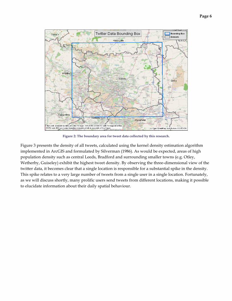
Tweets that can be geolocated to an area surrounding Leeds (as shown in Figure2) have been collected for the time period 22nd June – 12th October 2011. This consists of 290,215 individual tweets from 9,223 different users. The data are highly skewed; the top 10% most prolific users (922) are responsible for 78% of the total tweets (227,652) and 28% of the users (2,612) only generate one tweet. Although some of the tweet data clearly originate from businesses – examples include advertising cars or night club events – examination of the data reveals that the great majority of messages have been generated by real people. Although formal cleaning routines will be required if the data are to be used as model inputs, in the analyses later we focus on individual user behaviour and thus disregard superfluous data.

Figure 2: The boundary area for tweet data collected by this research.

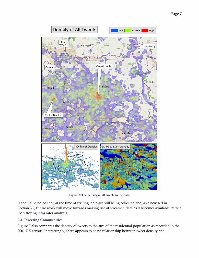
Figure 3 presents the density of all tweets, calculated using the kernel density estimation algorithm implemented in ArcGIS and formulated by Silverman (1986). As would be expected, areas of high population density such as central Leeds, Bradford and surrounding smaller towns (e.g. Otley, Wetherby, Guiseley) exhibit the highest tweet density. By observing the three-dimensional view of the twitter data, it becomes clear that a single location is responsible for a substantial spike in the density. This spike relates to a very large number of tweets from a single user in a single location. Fortunately, as we will discuss shortly, many prolific users send tweets from different locations, making it possible to elucidate information about their daily spatial behaviour.

Figure 3: The density of all tweets in the data.

It should be noted that, at the time of writing, data are still being collected and, as discussed in Section 3.2, future work will move towards making use of streamed data as it becomes available, rather than storing it for later analysis.

2.3 Tweeting Communities

Figure 3 also compares the density of tweets to the size of the residential population as recorded in the 2001 UK census. Interestingly, there appears to be no relationship between tweet density and

population density and this is verified by the scatterplot in Figure 4. This finding is somewhat unexpected because, given the obvious tweet density spikes around population centres, a relationship to residential population would be an understandable assumption. The fact that tweets do not correlate to residential density is encouraging as it suggests that twitter data could be used as a means of improving non-residential population estimates which are extremely difficult to estimate from traditional sources such as censuses. On the other hand, it could be simply that the use of tweets as the independent variable allows a small number of randomly located high volume users to influence this pattern, and that an ability to discriminate between tweets and tweeters – in particular, to define the normal residence for tweeters/ users – could help to refine this pattern. Section 3.2 will discuss this in more detail.

Figure 4: The number of tweets and the number of people (from the UK census) in each output area.

Further information about where tweets originate from, which will be extremely valuable in assessing how representative the data are of the whole Leeds population, can be found by examining the geodemographic profiles of the areas that the tweets are located in. The output area classification (OAC: Vickers and Rees, 2007) is a public domain classification using 2001 census data. The classification uses 41 separate census variables to partition the population into distinct socio-economic groups. Its most detailed level identifies 52 distinct sub-groups which in turn nest into 21 groups and 7 super-groups. To assess which groups have the largest number of tweets, Table 1 provides analysis of the number of tweets in each of the seven super-groups. The ratio of tweet proportions to OAC group proportions is indexed so that OAC groups with index values above 100 have more tweets than would be expected if tweets were distributed evenly across the whole city and those with an index under 100 have fewer tweets than would be expected.

Table 1: The number of tweets originating from different OAC groups in Leeds.

Counts Proportions OAC Group Tweet

s Group

s Tweet

s Group

s Index

2 - City Living 34482 211 0.268 0.087 309.5 3 - Countryside 4440 62 0.034 0.025 135.6 7 - Multicultural 16883 273 0.131 0.112 117.1 6 - Typical Traits 26283 571 0.204 0.234 87.2

5 - Constrained by Circumstances

19818 443 0.154 0.182 84.7

4 - Prospering Suburbs 17524 530 0.136 0.217 62.6 1 - Blue Collar 9349 349 0.073 0.143 50.7 Grand Total 128779 2439 1 1

Interestingly, ‘city living’ areas have three times as many tweets in them than would be expected if tweets were distributed evenly; a considerable amount. This adds support to the finding that most tweets emerge from non-residential areas because this group largely represents city-centre communities. However, as Section 3.2 will discuss, the subset of users who produce the largest number of tweets do not follow this pattern so strongly. Table 1 also exhibits a notable dip in tweeting activity in areas characterised by a high concentration of elderly (‘prospering suburbs’), manual employment (‘blue collar’) and deprived (‘constrained by circumstances’) populations.

2.4 Analysis of the Content of Messages

In addition to exploring the volume of tweets that originate from the different socio-deomgraphic groups, it is also illuminating to explore the locations of different words used in tweets. Research along these lines could help us to understand whether people use different types of words in different situations (e.g. at home or at work) and hence provide a means of identifying the type of activity that a person is engaged in.

The research begins by identifying all the unique words that are used in all the tweets in the dataset (note that, as with the previous analyses, tweets originating from outside the Leeds boundary are discarded). Here a ‘word’ is defined as a series of alphabetic characters surrounded by non-alphabetic characters (including whitespace).

Once unique words have been identified it is possible to find their locations (by examining the tweets in which they appear) and then map these distributions – as in Figure 5, in which clear patterns begin to emerge. For example, the results for the word ‘bar’ and ‘sleep’ are very different, as we would expect, but even this simple case is suggestive for some of the possibilities for connecting semantic and behavioural analyses – i.e. that the spatial patterns of daily living (sleep) and leisure time (bar) are somewhat different.

This analysis can be extended through a geodemographic analysis which profiles each word across the associated OAC communities. As with Section 2.3, the ratio of word proportions to OAC group

proportions is indexed to account for the relative prevalences of different OAC groups. Finally, the gini1 coefficient was calculated for each word to determine which words are the least dispersed across the community groups – and hence which are the most strongly associated with particular groups. Table 2 presents the results of the analysis for a selection of words that occur commonly, have relatively high Gini values and are potentially representative of a person’s activity. There are over 94,000 unique words so an exhaustive list of all words cannot be included.

Figure 5: The densities of some of the words identified in Table 2

1 The gini coefficient is a measure which is commonly applied to understand patterns of concentration in socio-spatial data – for example in the study of income inequalities (e.g. Deininger and Squire, 1996). In this work, a bespoke Python application – that made use of the gini function implemented in the R statistical package (following Handcock and Morris, 1999) – was written and applied to the twitter data.

Table 2: Results of the Gini analysis: the proportions of words that occur in each of the seven OAC groups. The OAC group names are: Blue collar (1); City living (2); Countryside (3); Prospering suburbs (4); Constrained by circumstances (5);

Typical Traits (6) and Multicultural (7)

Word GiniIndex Total Count

OAC Group Indices

1 2 3 4 5 6 7 railway 0.828 1147 34 1023 7 3 0 24 0 busines

s 0.640 444 50 724 122 12 68 31 42

bar 0.637 599 28 714 97 28 31 67 39 google 0.617 618 24 498 25 25 210 28 26 leeds 0.565 14001 23 607 158 58 54 43 68

lol 0.397 4192 46 145 115 45 73 66 351 today 0.394 4343 34 187 77 38 54 229 48 work 0.365 2282 53 345 64 52 97 100 78 job 0.364 574 63 338 74 46 129 71 89

fuck 0.312 704 63 278 193 67 104 60 129 sleep 0.299 849 65 278 214 73 90 84 84

Some of the results are as would be expected; the word “railway”, for example, occurs more than 100 times as often in the City Living group than would be expected if words were distributed evenly across social groups. This is because Leeds railway station is located in a City Living group. In fact, most words occur in City Living groups which supports the findings in Section 2.3 (future research will explore normalisation of the data further to remove this bias). Therefore it is extremely interesting that the word “google” has a high occurrence rate in Constrained by Circumstances groups, the words “business”, “leeds” and “sleep” are often used in Countryside groups, “lol” is used regularly in Multicultural groups and “today” is used in Typical Traits communities more than any other.

There are a number of ways that spatial word distributions could be explored further. Firstly, it would be interesting to disaggregate the data by time to gauge whether or not certain words exhibited temporal clustering. For example, if spatio-temporal clusters of words can be found around large cultural attractors (e.g. nightclubs) then this might be an indication of behaviour that holds in other situations as well (such as a person who attends a residential party rather than visiting their regular nightclub but whose use of language is consistent in both situations). Furthermore, by first estimating where the Twitter users live (see Section 3.3 for example) it would be possible to associate word usage to the places that people live, rather than where the tweets themselves originate. In this manner it could be possible to classify words and phrases demographically to explore how the use of language varies socially. Similarly, by linking the data to a classification of individual people or households (e.g. Malleson and Birkin, 2011) it would become possible to explore the individual socio-demographic differences in language use. All this would be invaluable when creating an individual-level model of urban dynamics in terms of classifying behaviour and calibrating to social data.

2.5 Temporal Patterns

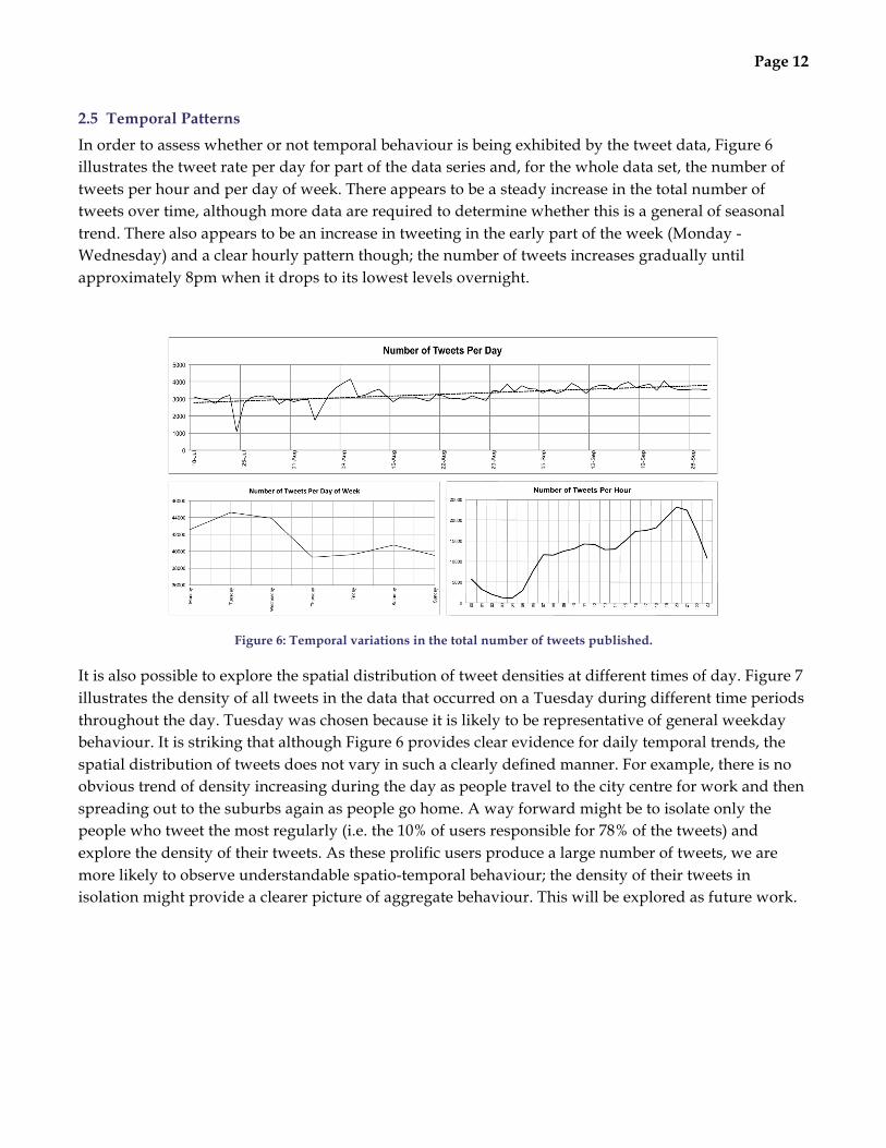
In order to assess whether or not temporal behaviour is being exhibited by the tweet data, Figure 6 illustrates the tweet rate per day for part of the data series and, for the whole data set, the number of tweets per hour and per day of week. There appears to be a steady increase in the total number of tweets over time, although more data are required to determine whether this is a general of seasonal trend. There also appears to be an increase in tweeting in the early part of the week (Monday - Wednesday) and a clear hourly pattern though; the number of tweets increases gradually until approximately 8pm when it drops to its lowest levels overnight.

Figure 6: Temporal variations in the total number of tweets published.

It is also possible to explore the spatial distribution of tweet densities at different times of day. Figure 7 illustrates the density of all tweets in the data that occurred on a Tuesday during different time periods throughout the day. Tuesday was chosen because it is likely to be representative of general weekday behaviour. It is striking that although Figure 6 provides clear evidence for daily temporal trends, the spatial distribution of tweets does not vary in such a clearly defined manner. For example, there is no obvious trend of density increasing during the day as people travel to the city centre for work and then spreading out to the suburbs again as people go home. A way forward might be to isolate only the people who tweet the most regularly (i.e. the 10% of users responsible for 78% of the tweets) and explore the density of their tweets. As these prolific users produce a large number of tweets, we are more likely to observe understandable spatio-temporal behaviour; the density of their tweets in isolation might provide a clearer picture of aggregate behaviour. This will be explored as future work.

Figure 7: The density of all tweets produced on a Tuesday.

Fortunately, because the data are available at the level of the individual person, it is possible to analyse individual users in detail without the reliance on aggregate patterns for an understanding of the spatio-temporal dynamics inherent in the data. The following section will explore this avenue in more detail.

3 Identifying Behaviour

3.1 Evidence for Theoretical Principles

In the introduction we examined the idea of Hägerstrand’s space-time prisms, which in practice are manifest as individual space-time paths. By observing the spatio-temporal locations of individuals’ tweets, it is a relatively straightforward matter to monitor the space-time paths of a large number of actors as they move around the urban environment. These data have the important characteristic that

they, for the most part, represent data at what Hornsby and Egenhofer (2002) refer to as a high granuality. Exploring space-time paths – or “lifelines” (Hornsby and Egenhofer, 2002) – with a high granularity makes it possible to explore highly detailed movements (such as making a single journey from 09:00–09:30 on a Tuesday) rather than more aggregate patterns (such commuting from one area to another in the morning). This level of granularity is essential for modelling the phenomena associated with dynamic urban systems.

For example, if we assume that a user’s ‘home’ is the place where they publish the largest number of tweets (Section 3.2 discusses this assumption in more detail) then Figure 8 is able to illustrate the distance that a single user travels away from home over the course of 112 days. It appears that they remain at home until 07:00 when they travel approximately 2.5km, returning home at 16:50. This diagram is effectively a representation of what time geography would refer to as a ‘space-time path’ (i.e. an individual section through the space-time prism) and could be used to better understand the constraints under which a particular user must operate. Over time, for example, it could be possible to estimate average speed of travel for different journeys and hence the type of transport that the user employs. Information of this sort would be extremely useful for the calibration of an agent-based simulation.

Figure 8: The distance from home over a short period of time for a single user.

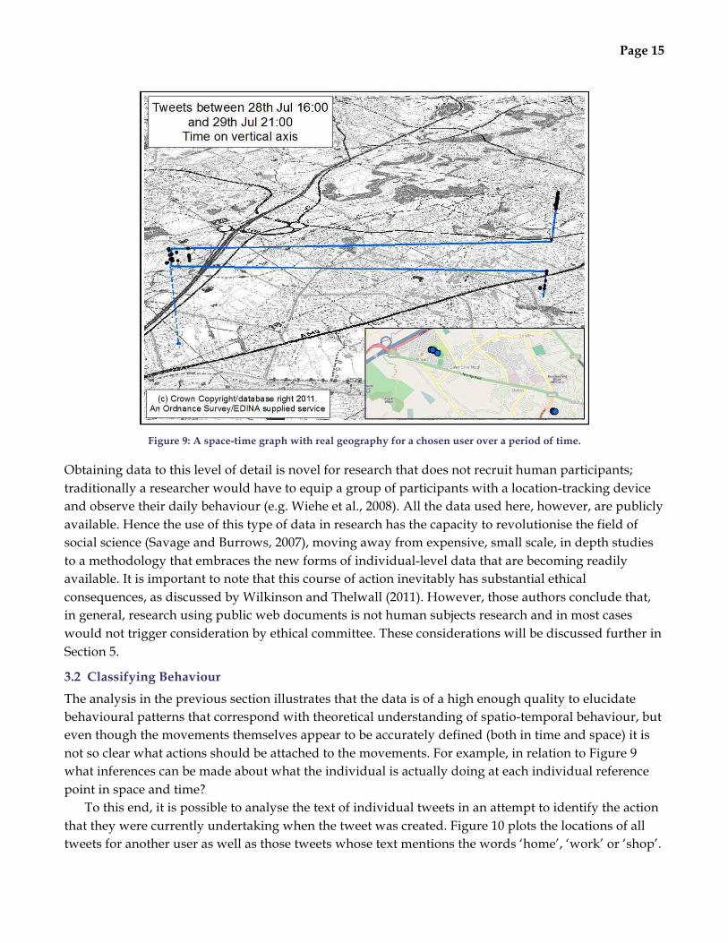
Given the richness of the data it is possible to extend this analysis and generate a complete 3D space-time prism constrained to a real-word geography, as illustrated by Figure 9. Visualising the data in this manner shows that it holds great promise for modelling travel behaviour. The two locations are linked by a major road which would most likely be used by the user if they had access to a car. Or, alternatively, by comparing the journey to local bus timetables or real-time bus location information it would be possible to predict, given the known time interval that the journey occurred in, whether public transport was used instead.

Figure 9: A space-time graph with real geography for a chosen user over a period of time.

Obtaining data to this level of detail is novel for research that does not recruit human participants; traditionally a researcher would have to equip a group of participants with a location-tracking device and observe their daily behaviour (e.g. Wiehe et al., 2008). All the data used here, however, are publicly available. Hence the use of this type of data in research has the capacity to revolutionise the field of social science (Savage and Burrows, 2007), moving away from expensive, small scale, in depth studies to a methodology that embraces the new forms of individual-level data that are becoming readily available. It is important to note that this course of action inevitably has substantial ethical consequences, as discussed by Wilkinson and Thelwall (2011). However, those authors conclude that, in general, research using public web documents is not human subjects research and in most cases would not trigger consideration by ethical committee. These considerations will be discussed further in Section 5.

3.2 Classifying Behaviour

The analysis in the previous section illustrates that the data is of a high enough quality to elucidate behavioural patterns that correspond with theoretical understanding of spatio-temporal behaviour, but even though the movements themselves appear to be accurately defined (both in time and space) it is not so clear what actions should be attached to the movements. For example, in relation to Figure 9 what inferences can be made about what the individual is actually doing at each individual reference point in space and time?

To this end, it is possible to analyse the text of individual tweets in an attempt to identify the action that they were currently undertaking when the tweet was created. Figure 10 plots the locations of all tweets for another user as well as those tweets whose text mentions the words ‘home’, ‘work’ or ‘shop’.

These words were used because they correspond with three of the five key behaviours for the agent-based model as outlined in Section 1 (and given the difficulty of the task, further investigation of ‘education’ and ‘leisure’ is postponed for later work).

Figure 10: Attempting to classify the behaviour of a single user based on a keyword search of their tweet contents.

The vast majority of tweets that mention ‘home’ occur in a very small area, which is also the area of the highest tweet density for the user (indicated on the map). There are also a large number of tweets along the main road between their home and the centre of Leeds so a fair assumption might be that the user works in the city centre. Both of these assumptions could be investigated further by examining the times that tweets were sent and verifying whether or not the times correspond to those that we would expect a person to be at home or at work.

It should be noted that, as Section 2.3 pointed out, most tweet data originate from non-residential areas. This casts doubt on using the data for behavioural modelling because it might be impossible to establish the main anchor point for a person’s travel behaviour: their home. However, it is likely that for the small subset of users who generate enough data for us to understand their travel behaviour (only 6% of users produce more than 100 tweets) most of their tweets will not originate from non-residential areas. This can be verified by Table 3 which provides the ratio index for the number of tweets in different communities for the 6% of users who generate more than 100 tweets. With a comparison to Table 1, it is clear that the index of tweets in ‘city living’ communities has reduced from 310 (more than three times as many tweets) to 250. This is encouraging as it suggests that it will be possible to estimate the home locations for the most important users (those with sufficient data to

analyse). Hence a safe assumption, at this stage, is that a person’s home location is that which has the greatest density of their tweets. Future work will, of course, aim to improve this assumption through the use of text mining or other methods (e.g. analysing the surrounding environment).

Table 3: The number of tweets generated by ‘prolific’ users (those 100 or more tweets in total) originating from different

OAC groups.

Counts Proportions OAC Group Tweet

s Group

s Tweet

s Group

s Index

2 - City Living 18775 211 0.216 0.087 249.8 7 - Multicultural 13703 273 0.158 0.112 140.9 3 - Countryside 2240 62 0.026 0.025 101.4

5 - Constrained by Circumstances

14672 443 0.169 0.182 93.0

6 - Typical Traits 18810 571 0.217 0.234 92.5 4 - Prospering Suburbs 12023 530 0.138 0.217 63.7

1 - Blue Collar 6651 349 0.077 0.143 53.5 Grand Total 86874 2439 1 1

In terms of identifying a persons’ actions, a naïve keyword search. The most obvious drawback is that the ‘home’ location is the most common place for all tweets, even those that have been identified by ‘shop’ and ‘work’ key words. Hence simply searching for a key word is insufficient for establishing the action that the person was undertaking when they published the tweet. By analysing individual tweets it becomes obvious why this is the case. Table 4 provides some examples of tweets that include one of the chosen keywords but clearly cannot be classified by that activity. The names of other twitter users have been replaced by ‘[user]’ to preserve anonymity.

Table 4: Examples of the text captured with a keyword search.

Word Text Work “Cheese on toast for breakfast before I venture into the rain to

go to work.” “Does anyone fancy going to work for me? Don’t want to get

up” “Beer does work. Having blurted out to a girl that she is the spit

of [user] I’ve bagged her number. And she likes rugby! ” Home “Pizza ordered ready for ones arrival home”

“[user] that’s not a nice thing to say about your home. It did

look grim at that time of night though” “Ah the good old sight of The White Rose shopping centre.

Means I’m nearly home” “Home time at long last”

Shop “Ah the good old sight of The White Rose shopping centre. Means I’m nearly home”

“[user] haha well played. Was she taking him shopping? ” “Are the shops in town open today? I really need a hammer,

picture hooks, Stanley knife and spirit level. DIY bonanza day”

Although the examples in Table 4 illustrate where the keyword search fails to classify behaviour, it also suggests that most text could actually be classified by a more intelligent routine. Phrases such as “Don’t want to get up”, and “I’m nearly home” are indicative of clearly defined activities – preparing to leave home or arrive home respectively. Also, through a manual inspection of tweets it was possible to identify when the user was spending time in a local pub and when they were shopping in nearby town centres.

Hence an advanced algorithm that analysed the entire text rather than single words and also considered tweet location should be able to successfully classify a large number of the data points. There is a rapidly growing body of literature that apply techniques such as sentiment analysis to classify meaning or action in crowd-sourced data. See, for example, Gomide et al. (2011), Russell (2011), Ananiadouet al. (2010), and Gelernter et al. (2011).

Although we are aware of no published work that combines textual and spatio-temporal clustering methods, social data mining techniques – see, for example, Russell (2011) – offer a strong starting position.

3.3 Establishing Social Networks

It is inevitable that a realistic model of city dynamics should include some representation of social networks. Davis Jr et al. (2011), for example, use friendship networks to attempt to spatially locate tweets that otherwise have no location information. There are two mechanisms for users to refer to each other in their tweets:

• A user can ‘mention’ someone else by preceding the recipient’s username with an ‘at’ symbol (@) anywhere in the tweet. For example, the hypothetical tweet “Having coffee with @Sam” mentions another user called ‘Sam’.

• A user can also ‘reply’ directly to another user by starting the text with that person’s user name. For example: “@Sam I’m on my way?” is a message specifically for the user ‘Sam’.

These different mechanisms have consequences for how messages are displayed on users’ twitter pages but otherwise both types of messages are the same (they are collected identically when gathering tweets from the Streaming API). Hence it is possible to parse tweet data and construct different types of

social network. At present, we do not differentiate between messages that are addressed directly to a specific individual (‘replies’) or those that merely mention antother user (‘mentions’) but this is a clear avenue for future work. A preliminary procedure for this research assigned a single ‘home’ location to each user by calculating – using the Kernel Density Estimation algorithm – the most dense point for all of the user’s tweets. Although in some cases this point will not represent a person’s home, a short manual inspection suggests that the procedure is largely successful. Figure 11 illustrates the social network that is generated after assigning individual points as users’ homes. Each link indicates that one user has mentioned the other and the strength of the link indicates the total number of separate mentions. At this stage the network is directionless so does not indicate which user wrote the tweet.

Figure 11: The social network constructed from the twitter data. The a-spatial network (produced using the GUESS

software (Adar, 2006)) focusses on a sub-graph surrounding one user in particular. This sub-graph has also been mapped spatially. Each node is the ‘home’ location of a single user and the edges represent communications (one or many).

From Figure 11 it becomes clear that there are a large number of small, disconnected networks and a single much larger network. It would potentially be illuminating to explore the relationship between the size and shape of a user’s social network and the community classification of their estimated home location. However, the current social network is relatively sparse (it contains less than 800 separate edges) so a larger data set will be collected prior to drawing any firm conclusions regarding social relationships in the data.

However, there are a range of potentially illuminating analyses that could be conducted once more data are available. By statistically measuring the network structure – using, for example, measures of connectivity and centrality – we could explore:

• The relationship to mobility and activities – do well-connected individuals tend to go to bars more often?

• The relationship to geodemographics – do multicultural individuals have bigger social networks than typical traits?

• Whether or not there general differences in the social networks found in different cities or countries.

There is also scope for more broadly exploring the relationship between physical and social networks. For example, there might be similarities between virtual communication and physical patterns of movement. This has obvious relevance for models that are inherently spatial but are backed by social networks such as models of disease outbreak.

4 Discussion: Towards an Agent-Based Model of Urban Dynamics

We have argued above that individual agents could prove to be the most effective way of representing entities and their behaviour patterns, especially when we are concerned with actions which are discrete in space and time – such as visiting a bar or restaurant. In the paper we have classified such behaviours into some broad types and aim to extend them to include all of the following: at home, at work, shopping, leisure and education. Note that of course much more detail could be introduced into many of these categories, so for example the behaviour patterns associated with a regular weekly shop for groceries could be very different to an occasional excursion for shoes or clothes. Activities undertaken at home could take a wide range of forms (gardening, sleeping, reading, cooking, and so on) – and we begin to speculate why these might be of particular interest to the analyst or policy-maker below. It is also worth noting however that the value of agent-based models in simulating the ‘slow dynamics’ associated with more strategic decisions (e.g. moving home) have also been championed in certain quarters (Jordan et al., 2011).

We have begun to develop illustrations of real activity patterns which have a distinct resonance with the theoretical frameworks of behavioural geography and time geography. Through detailed analysis of individual entries in a corpus of geo-located twitter messages it has been shown that constrained intra-urban movement patterns, e.g. from home to work to shop and home again, and so on, can be detected and illustrated. In order to extend this work in the direction of a more general framework for agent-based modelling of urban dynamics, at least two further steps are required:

• First, it is not feasible to attempt the detection of behaviour patterns in a data set with hundreds of thousands of entries through manual inspection. To take this further step requires some kind of automated mining procedure which is able to infer, with reasonable confidence, what a person is doing at a particular point in time; or which common sets of entries together imply that a subject is ‘at home’ or ‘at work’. There are some parallels in the text mining software which has been under development for some time. For example, the National Centre for Text Mining (NaCTeM) is currently investigating the application of text mining services and software tools to problems relating to biomedical research and drug discovery, social history and language

technologies (http://www.nactem.ac.uk/research.php; Ananiadou et al, 2010). The use of algorithms to detect sentiment in financial markets is surely a subject of interest, and not just in popular fiction (Harris, 2011). Indeed the Guardian Newspaper has commissioned and published a range of analyses of social network data relating to the London riots of 2011 (Lewis, 2011) with a view to a better understanding of the causes, dynamics and chronology of these events. For all this, one suspects that the software tools available are still far from maturity and that further work is needed to construct a set of methods which can extract maximum value from information which is specifically geo-temporal in its character – again the recurrence of activity at particular locations such as home, work, or a preferred leisure spot; or in the context of urban unrest then perhaps the gathering and dispersal of groups that the notion of a riot suggests.

• Secondly, the kind of data which comes from crowds is not the subject of regular stratified samples, and it is not controlled for quality, completeness and accuracy. We have already seen in our sample dataset that there is an enormous skew in which a very large portion of the data is generated by a small number of prolific individuals. In order to smooth out the significant biases in these data we require at the least some powerful reweighting tools. The idea of geodemographics may have some currency here. Whenever a tweet is geo-located then this location itself could be used as a basis for estimating the character of the individual from whom this message is sourced. Linking the twitter data to some kind of spatial microsimulation model would be a more refined way of attempting something similar. In this case we assume that our target class is not a homogeneous geodemographic type at each location but a distribution of individuals whose profile of socio-economic and demographic characteristics can be estimated. This approach could be made more powerful still if appropriate inferences could be made to qualify the characteristics of the individuals in the twitter data. For example, is it possible to make inferences about age or ethnicity from the names posted by individuals – certainly gender should be identifiable with reasonable confidence. Maybe it is possible to identify family and relationship status from textual analysis, while the use of specific words and phrases could be associated with particular ages or social and income groups.

In order to articulate this model framework more fully, we propose that a population of agents could be initiated through an existing microsimulation model. This population would be provided with a set of attributes which can now be regarded as reasonably standard i.e. age, gender, ethnicity, occupation, household composition, health status – see, for example, Wu et al. (2010) or Malleson and Birkin (2011). Other characteristics can be synthesised if necessary. The dynamics of a spatial microsimulation of this type can be analysed over long time periods using demographic projection methods (Wu et al., 2008) in which the transition between locations and states is monitored in discrete annual time intervals. What we suggest here is that the behaviour of a set of agents could be traced over a much finer timescale, perhaps even dividing each day into individual hourly segments. At each point in time both the location and current activity of the agent would be simulated (where at its most straightforward these activities comprise our standard categories of home, work, shop, leisure etc). From one time period to the next, the transition probabilities are estimated using a function of the form:

P(j,b,t+1 | i,a,t) = f (a,t,t*,y0) (1)

In other words, the probability that an individual at location i, engaged in activity a at time t moves to location j and activity b at time t+1 is related to the current activity (a), the time of day (t), the length of time over which the current activity has been conducted (t*) and the characteristics of the individual agent (y0). Through the implementation of the generic textual and spatial analyses which have been

described above we would be optimistic about the possibility of establishing a reasonable approximation to these functional relationships.

The idea of data linkage and microsimulation could itself be extended to examine the synthesis not just of traditional sources such as the census and government surveys, but also to other new forms of data. For example, Savage and Burrows (2007) particularly note the rise of commercial data sources, including lifestyle data, as a potentially valuable source. If twitter data could be linked to a microsimulation, then it could also be linked to something like a lifestyle database (Thompson et al., 2012), for example to add extra intelligence about how people actually spend their time (and money) whilst at home, or out and about in the urban system. This kind of information (enjoys reading, gardening etc) could be of value not just to the marketers of retail businesses, but to planners of services such as libraries, civic advice centres, health clinics etc. For example, if the prevalence of smoking is high then maybe there is a greater need for education or intervention (cfTomintz et al., 2009).

There is also some considerable scope for integrating other social network data sources (e.g. Facebook and FourSquare) as well as similar commercial data. For example, Stefanidis et al. (2011) propose a framework for collecting and analysing social data from multiple sources and Nagurney&Tranos (in press) make use of anonymised mobile telephone data better understand who social behaviour varies spatially in the Netherlands.On the other hand, it is understandable that many researchers have reservations about the apparent lack of quality control in crowd-sourced datasets of this type. For example, census data in the UK and elsewhere has almost universal population coverage and has full backing from the national government to ensure a minimum of misreporting. Other social surveys, whether academic, commercial or governmental, are typically rigorously stratified and carefully administered through a variety of channels to guarantee robust responses from willing participants. In this context, it could be objected that social media are biased in their coverage, offer distorted behavioural profiles, use collection methods that are ethically dubious, and have content which is poorly aligned to the needs of the research community. There is an element of truth in each of these, but none exposes a critical limitation in the data:

a) Bias. It is true that people who tweet are not representative of the population as a whole. This has been demonstrated in our geodemographic analysis of Section 2.3, which complements other evidence about the demographic profile of users (e.g. 80% of tweets by individuals in their 20s and 30s). However, when compared to a blue chip source such as the National Travel Survey (NTS) in the UK, potential advantages become apparent, The NTS, for example, collects data for about 10,000 individuals each year, wheras the data used here captures about 10,000 individuals in Leeds alone every month. There is every chance that even undersampled demographics such as the elderly are more represented in volume terms in the Twitter data than in the NTS. Commercial organisations routinely use reweighting techniques to make surveys fully representative against a national population (e.g. Thompson et al, 2010) – in effect, stratification is applied to the sample after its collection, rather than

beforehand as in much social research and market research. In the models which are proposed here, microsimulation would provide an effective base for reweighting activity data from Twitter. This could be based initially on a crude geodemographic matching process, although we are also exploring the use of third party data (Acxiom ROP) to generate robust social and demographic profiles of social media users.

b) Behavioural distortion. It is clear intuitively, and also from the evidence presented above (Figure 6c), that some activities are much more likely to provoke tweets than others. Again, we believe it is possible here to triangulate against other sources to get a more accurate picture. For example, once the modelling process which we outline here is complete then flows of employees to workplaces and catchment areas for schoolchildren would be generated. These models could then be calibrated against journey to work data from the 2011 census, and against the National Pupil Database (which contains full pupil flows in England) to reduce model distortions. In effect, this is a powerful model-based approach to the problem of reweighting and stratification of the data. It is also possible that panel surveys could be introduced at some point to detect and inform the relationship between activity patterns and engagement with social media including tweets.

c) Ethics. We have noted already that there are some ethical concerns about the use of social media data for purposes other than that for which it was originally intended. However the streaming APIs which generate the data which has been presented here operate using randomised 1% samples of the full data set which is handled by the twitter server. Although precise details of names, locations and message content can be obtained, these will not usually be required for the kinds of analysis advocated within this paper. Simple protocols can be invoked to ensure that private data is never shared or published, and in principle these protocols could be extended to give extra protection through spatial aggregation or randomisation of the underlying data. Similar work is routinely carried out with other forms of sensitive data such as that of victims of crime (Chainey and Ratcliffe, 2005). Although it could be argued that many core uses of twitter, such as stalking and hate messages against named individuals, is distasteful and ethically dubious, the academic research community should have both the skills and responsibility to sidestep any worries of this nature.

d) Poor alignment of content. As we showed in Section x, it is not straightforward to extract usable information content from twitter messages. This is true regarding both activity patterns (e.g distinguishing ‘ready to go home’ from ‘at home’) and social networks (one might tweet an opinion about Barack Obama without being a personal friend). A problem here is that algorithms for the extraction of content from text messages are still rather unsophisticated. However significant effort is being invested in the development of more sophisticated techniques – for example, it is now possible to perform analyses of ‘sentiment’ to extract the strength and direction of opinion about topics such as public attitudes to crime and policing (SentiStrengthreference). It seems inevitable that text mining tools of this ilk will become increasingly reliable as more work is devoted towards their development.

In general, although this paper has mostly focused on behavioural modelling as an intellectual

challenge, the potential practical benefits in pursuing this research agenda are substantial. Whilst it may be convenient to assume that urban environments are slow moving and well-structured (and thus, for example, that something like a decennial population census can adequately capture its essential characteristics) in practice the daily ebb and flow of the population is surely critical in understanding

its needs, whether for healthcare, education, crime prevention, retailing, or any of the myriad of infrastructure and services which are critical to the lubrication of the urban ecosystem.

5 Conclusion

This paper has explored the contents of new social networking data from Twitter to gauge its applicability to a model of urban dynamics. Although there will be substantial challenges for identifying a person’s actions from their individual tweets, the problems are not insurmountable. Much of the data have high-resolution coordinates associated with them which lends them nicely for the calibration and validation of a model. Furthermore, these types of streaming data sources could potentially be used as a means of improving social models in situ as they are produced in a similar to that used in other fields such as meteorology (Collins, 2007). Observing social systems over time is a “fundamental problem” (Janssen and Ostrom, 2006) which this type of data might offer a solution to.

Clearly there are considerable ethical issues surrounding the use of these data that must be addressed. The traditional means of obtaining such high quality spatial/behavioural data would be through a formal qualitative interview process in which the subject gave their consent for the research and where any data collected were strictly guarded by data protection / privacy legislation. However, this approach is not feasible with the use of crowd-sourced data; even if it were possible to contact the individuals directly, the sheer quantity of data prohibits this. Also, even though the data is publicly available and users must opt-in to the location services that publish their location it is not clear whether or not they are fully aware of the implications. For example, it is not clear whether the users depicted in Figures 9 and 10 are aware of how much data they have made available to the public. Hence the need to, at this stage, hide user names and draw maps at a resolution that makes it impossible to identify individual houses.

The potential impact of Twitter and other social media data for the analysis of spatial systems is wide-ranging. However within the modelling framework proposed here the two most significant areas for immediate exploration are: developing spatial text mining techniques to identify people’s actions from their tweet data and working towards a formal means of updating a working agent-based model with streamed social data. Also, by searching for user names in the text of tweets it is possible to construct a social network of Twitter users who communicate via tweets – work along these lines could potentially be extremely interesting.

References Adar, E. (2006). GUESS: a language and interface for graph exploration. In CHI, Montreal, Canada. Ananiadou, S., Pyysalo, S., Tsujii, J. and Kell, D. B.. (2010). Event extraction for systems biology by text mining

the literature. Trends in Biotechnology, 28(7), 381-390 Ballas, D. and G. Clarke (2001). The Local Implications of Major Job Transformations in the City: A Spatial

Microsimulation Approach. Geographical Analysis 33(4), 1–21. Batty, M. (2005). Agents, cells, and cities: new representational models for simulating multiscale urban dynamics.

Environment and Planning A 37, 1373–1394. Bell, G., T. Hey, and A. Szalay (2009). Beyond the data deluge. Science 323, 1297–1298. Birkin, M. and G. Clarke (2011). Spatial Microsimulation: challenges of dealing with demographics at the small

area level. In J. Stillwell and M. Clarke (Eds.), Population Dynamics and Projection Methods: Essays in Honour of Philip Rees, pp. 193–208. Berlin: Springer.

Birkin, M., A. Turner, and B. Wu (2006). A synthetic demographic model of the UK population: Progress and problems. In 2nd International Conference on e-Social Science, Manchester.

Bonabeau, E. (2002). Agent-based modeling: Methods and techniques for simulating human systems. Proceedings of the National Academy of Sciences 99(90003), 7280–7287.

Burgess, E. W. (1925). The Growth of the City. In R. E. Park, E. W. Burgess, and R. D. McKenzie (Eds.), The City, pp. 47–62. University of Chicago Press.

Cheng, Z., J. Caverlee, and K. Lee (2010). You are where you tweet: a content-based approach to geo-locating twitter users. In Proceedings of the 19th ACM international conference on Information and knowledge management - CIKM ’10, pp. 759–768. New York, New York, USA: ACM Press.

Collins, M. (2007). Ensembles and probabilities: a new era in the prediction of climate change. Philosophical Transactions of the Royal Society A 365(1857), 1957–1970.

Chainey, S., & Ratcliffe, J. (2005). GIS and Crime Mapping. Chichester: John Wiley and Sons. Davis Jr, C. A., G. L. Pappa, D. R. R. de Oliveira, and F. de L Arcanjo (2011). Inferring the Location of Twitter

Messages Based on User Relationships. Transactions in GIS 15(6), 735–751. Deininger, M. and Squire, J. (1996) A new data set measuring income inequalities, World Bank Economic

Review, 10 (3), 565-591. Gelernter, J., & Mushegian, N. (2011). Geo-parsing Messages from Microtext. Transactions in GIS, 15(6), 753–

773. Golledge, R. G., L. A. Brown, and F. Williamson (1972). Behavioural approaches in geography: an overview.

Australian Geographer 12(1), 59–79. Gomide, J., Veloso, A., Meira, W., Almeida, V., Benevenuto, F., Ferraz, F., & Teixeira, M. (2011). Dengue

surveillance based on a computational model of spatio-temporal locality of Twitter (pp. 1–8). Proceedings of the ACM, Koblenz, Germany.

Goodchild, M. (2007). Citizens as sensors: the world of volunteered geography. GeoJournal 69, 211–221. Hägerstrand, T. (1970). What about people in regional science? Papers in Regional Science 24, 6–21. Handcock, M. and M. Morris (1999). Relative Distribution Methods in the Social Sciences, New York: Springer-

Verlag Harris, R. (2011). The Fear Index. London: Hutchinson. Hornsby, K., & Egenhofer, M. (2002). Modeling Moving Objects over Multiple Granularities. Annals of

Mathematics and Artificial Intelligence, 36, 177–194. Janssen, M. A. and E. Ostrom (2006). Empirically Based, Agent-based models. Ecology and Society 11, 1–13. Jordan, R., M. Birkin, and A. Evans (2011). Agent-based Simulation Modelling of Housing Choice and Urban

Regeneration Policy’. In T. Bosse, A. Geller, and C. Jonker (Eds.), Multi-Agent-Based Simulation XI, pp. 152–166. Berlin: Springer.

Keith, C. C. and L. J. Gaydos (1998). Loose-coupling a cellular automaton model and GIS: long-term urban growth prediction for San Francisco and Washington/Baltimore. International Journal of Geographical Information Science 12, 699–714.

Lewis, P. (2011, September). Reading the Riots study to examine causes and effects of August unrest. The Guardian.

Malleson, N. and M. Birkin (2011). Towards victim-oriented crime modelling in a social science e-infrastructure. Philosophical Transactions of the Royal Society A: Mathematical, Physical and Engineering Sciences 369(1949), 3353–3371.

Miller, E., J. Douglas Hunt, J. Abraham, and P. Salvini (2004). Microsimulating urban systems. Computers, Environment and Urban Systems 28(1-2), 9–44.

Miller, H. J. (2004). Activities in Space and Time. In P. Stopher, K. Button, K. Haynes, and D. Hensher (Eds.), Handbook of Transport 5: Transport Geography and Spatial Systems. Pergamon/Elsevier Science.

Parker, D. C., S. M. Manson, M. A. Janssen, M. J. Hoffmann, and P. Deadman (2003). Multi-Agent Systems for the Simulation of Land-Use and Land-Cover Change: A Review. Annals of the Association of American Geographers 93(2), 314–337.

Pred, A. (1967). Behaviour and Location: Foundations for a Geographic Dynamic Location Theory. Lund Studies in Geography Series B. Lund.

Prothmann, H., F. Rochner, S. Tomforde, J. Branke, C. Müller-Schloer, and H. Schmeck (2008). Organic Control of Traffic Lights. Lecture Notes in Computer Science 5060(Chapter 19), 219–233.

Putman, S. (1983). Integrated urban models Policy analysis of transportation and land use. London: Pion. Russell, M. (2011). Mining the Social Web. Analyzing Data from Facebook, Twitter, LinkedIn, and Other Social

Media Sites. O’Reilly Media, Inc. Savage, M. and R. Burrows (2007). The Coming Crisis of Empirical Sociology. Sociology 41(5), 885–899. Silverman, B. W. Density Estimation for Statistics and Data Analysis. New York: Chapman and Hall, 1986. Stefanidis, A., A. Crooks, and J. Radzikowski (2011). Harvesting ambient geospatial information from social

media feeds. GeoJournal. Thompson, C., G. Clarke, M. Clarke, and J. Stillwell (2012). Modelling the Future Opportunities for Deep

Discount Food Retailing in Great Britain. International Journal of Retail Distribution and Management (forthcoming).

Tomintz, M. N., G. P. Clarke, and J. E. Rigby (2009). Planning the Location of Stop Smoking Services at the Local Level: A Geographic Analysis. The Journal of Smoking Cessation 4(2), 61–73.

Vickers, D. and P. Rees (2007). Creating the UK national statistics 2001 output area classification. Journal of the Royal Statistical Society A 170, 379–403.

Wiehe, S. E., A. E. Carroll, G. C. Liu, K. L. Haberkorn, S. C. Hoch, J. S. Wilson, and J. D. Fortenberry (2008). Using GPS-enabled cell phones to track the travel patterns of adolescents. International Journal of Health Geographics 7(1), 22.

Wilkinson, D. and M. Thelwall (2011). Researching Personal Information on the Public Web: Methods and Ethics. Social Science Computer Review 29(4), 387–401.

Wu, B., M. Birkin, and P. Rees (2008). A spatial microsimulation model with student agents. Computers, Environment and Urban Systems 32(6), 440–453.

Wu, B. M., M. H. Birkin, and P. H. Rees (2010). A Dynamic MSM With Agent Elements for Spatial Demographic Forecasting. Social Science Computer Review 29(1), 145–160.

Yang, Y., P. Atkinson, and D. Ettema (2008). Individual space–time activity-based modelling of infectious disease transmission within a city. Journal of The Royal Society Interface 5(24), 759–772.

investigating the behaviour of twitter users to construct...

Documents