investigating the benefit of condition measurements for ... · degree project in investigating the...
TRANSCRIPT

Degree project in
Investigating the benefit of condition measurements for critical components
in power transmission systems
Johanna Gunhardson
Stockholm, Sweden 2013
XR-EE-ETK 2013:003
Electromagnetic EngineeringSecond Level, 30.0 HEC

2

3
ABSTRACT
This master thesis project has been conducted as a collaboration between Svenska Kraftnät and
the Royal Institute of Technology.
High demands are being put on all components in a transmission system to be available for
operation, making the allowed component down-time the limiting factor in the maintenance
budget for Svenska Kraftnät and other transmission system operators. By conducting condition
measurements that can be performed on-line, excessive down-times could be avoided in a step
towards an as efficient maintenance strategy as possible.
The approach of this thesis work has been to perform a case study for a population of
transmission grid circuit breakers, creating a model of the CBs’ lifetime which has then been
simulated with the aim of studying the benefit of periodic on-line condition measurements for
power system components. The main potential benefit examined is the decrease in total down-
time for the component population, in relation to the respective components’ criticality.
The conclusions of this thesis project are summarized below.
Replacing the periodic off-line preventive maintenance with on-line condition
measurements for the most critical circuit breakers in a power transmission system,
significantly diminishes the weighted overall down-time for all circuit breakers in the
system.
It is most preferable to use frequent intervals for condition measurements for a large
part of the circuit breaker population.
A maintenance strategy based on condition measurements is best motivated in cases
where the randomness of circuit breaker condition deterioration is high, the failure rate
is high, or condition measurements have low uncertainty, and least motivated in cases
where the conditions are the opposite.
Severe transient effects in average age of the component population may appear in
response to any changes in maintenance strategy (or the lack of it), having a harsh
impact for power system owners.

4

5
ACKNOWLEDGEMENTS
I would like to thank my supervisor at the RCAM research group at KTH, Patrik Hilber, for his
constant support in my work, regarding matters small and large and everything in between. I
would like to thank my supervisor at Svenska Kraftnät, Tommie Lindquist, for great direction and
input along the course of the project.
A big thank you also to Per Westerlund in the RCAM group for great attention to detail and for
helping me improve my methods.
Everyone in the RCAM group, that have become good friends to me, I would like to thank for
reminding me to take well-needed breaks, and of course for many laughs. A special thank you to
Johanna Rosenlind for exceptional brain-storming, helping me break through at some of the tough
moments in the project.
Another special thank you to Jenny Paulinder and Emil Andersson at Göteborg Energi Nät AB for
valuable insights into the challenges facing distribution system operators in questions regarding
maintenance and power system asset management.
These past months have taught me a lot regarding power grids, probably more even than I realize,
making me more and more impatient to start my career as a power system engineer. Thanks again
to everyone!

6

7
ENGLISH-SWEDISH DICTIONARY
English Swedish Description
3D simulation 3D-simulering The model varies the main variables according to
the model settings, running the simulation for
each of their possible combinations.
Availability Tillgänglighet The time a component is connected to the
network and in operation/ available for operation.
Circuit breaker (CB) Effektbrytare A mechanical switching device that may conduct
or break the current under normal operation and
that also can conduct, for a specified time, and
break currents under specified abnormal
conditions such as short circuits.
Condition Tillstånd A measure of how worn a component is. The
condition is good when the component is new,
and deteriorates with time and wear.
Condition based
maintenance
Tillståndsstyrt
underhåll
Makes use of the component’s estimated
condition [1] to determine when preventive
maintenance should take place.
Condition
measurement
Tillståndsmätning The estimation of a component’s condition
through periodic measurements (diagnostic
testing).
Condition
monitoring
Tillståndsövervakning Continuous on-line measurements of primary
equipment with the devices permanently installed.
[2]
Corrective
maintenance
Avhjälpande
underhåll
Carried out after a component failure in order to
restore the component to its required function.[1]
Critical component Kritisk komponent Important component to the overall function of a
system.

8
Critical transfer
sections
Kritiska
överföringssnitt,
“flaskhalsar”
“Bottle necks” in transmission system, limiting the
power transfer capability in a certain direction.
Decision process Beslutsprocess In this thesis referring to the decision of when to
schedule a replacement of a component.
Diagnostic testing Diagnostisk
mätning/test
The estimation of a component’s condition
through periodic measurements.
Down-time Tid ur drift Time when a component is not available for
service, while undergoing maintenance.
Equivalent age Ekvivalent ålder A measure of age combining a CB’s age and
number of performed operations.
Failure Fel, haveri A failed component is unable to perform all its
required functions.
Failure mode A Feltyp A Replacement is required to restore the CB to its
required function.
Failure mode B Feltyp B Repair to pre-fault condition is sufficient to restore
the CB to its required function.
Failure rate Felfrekvens The probability of a component failing.
Hazard rate Risknivå The probability of a component failing.
Importance Viktighet A measure of how critical a component is to the
overall system function.
Importance index Viktighetsindex A tool for determining a system’s components’
importance level in relation to each other.
Important CB Viktig brytare In this thesis a CB regarded as more critical to the
system.
Main variables Huvudvariabler QICB and MIICB, see Abbreviations and notations
below.
N-1 criterion N-1 kriteriet Deterministic criterion signifying that any single
component failure will not interrupt the system
function (delivering power to all load points)

9
Off-line Ur drift Equipment de-energized and disconnected from
network.[2]
On-line I drift Equipment energized and connected to
network.[2]
Operation Manöver
Drift
Opening or closing a circuit.
For instance, ‘operating a grid’ or ‘a component
being in operation’
Preventive
maintenance
Förebyggande
underhåll
Carried out with the aim of preventing component
failure.
Primary equipment Primärutrustning Components in a power grid with the main
function of transferring power, such as
transformers or over-head lines.
Reliability Tillförlitlighet The probability of a component performing its
required function during a specified amount of
time.
Reliability centered
maintenance
Funktionssäkerhets-
inriktat underhåll
Qualitative methodology with the purpose of
creating cost effective maintenance plans based
on probabilities and consequences of failure.
Repair Reparation In this thesis referring to restoring a failed CB to its
pre-fault condition.
Replacement Ersättning, utbyte Preventive repl. – in this thesis referring to the
scheduled replacement of a CB, in order to avoid
future failure.
Corrective repl. – In this thesis referring to the
replacement of a CB after failure.
Secondary
equipment
Sekundärutrustning Components in power systems that do not have
power transfer as their main function, such as
protection relays.
Single-point
simulation
Enpunktssimulering The model runs the simulation for one value each
of the main variables.

10
Time based
maintenance
Tidsstyrt underhåll Performed at periodic intervals.
Time out of service Tid ur drift Time when a component is not available for
service, while undergoing maintenance.
Transient Transient Diminishing oscillations that appear in response to
a step change, which in time settle.
Transmission
system/grid
Transmissionsnät,
stamnät
The back bone of a power grid, with the main
function of transferring large amounts of power
long distances.
Transmission
system operator
Stamnätsoperatör Organization responsible for the operation of a
transmission grid.
Unavailability Otillgänglighet The time a component is disconnected from the
network and not available for operation.
Unprioritized CB Oprioriterad brytare In this thesis a CB regarded as less critical to the
system.
Weighted […] Viktad […] In this thesis referred to results weighted
according to component importance.
ABBREVIATIONS AND NOTATIONS
Abbreviation/notation Description
ABAO As bad as old
af Age factor
AGAN As good as new
ageOps Age in operations
ageYears Age in years
CA Condition measurement (Condition assessment)
CB Circuit breaker
CBM Condition based maintenance
CM Corrective maintenance
cond Condition

11
Correlation a-d, A-D Correlation between main variables and 3D simulation output. See
section 6.2.
eqAge Equivalent age
ICB Important circuit breaker
ID Importance distribution, either
ID 1 – Importance unit
ID 2 – Importance ranking (1, 2, 3, 4, …)
ID 3 – Equal ranking (no importance weighting)
mCond Measured CB condition at CA
mEqAge Equivalent age of CB when CA takes place
MIICB Measurement interval for important circuit breakers – The number
of years between condition measurements for important breakers.
ops Operations
QICB Quota of important circuit breakers – The percentage of the total
amount of circuit breakers in the population to be regarded as
important
PM Preventive maintenance
RCAM Reliability centered asset management
RCM Reliability centered maintenance
RTF Run to failure (maintenance philosophy)
SvK Svenska Kraftnät, Swedish TSO
TBM Time based maintenance
TSO Transmission system operator
UCB Unprioritized circuit breaker
WRR Weighted replacement ratio = Ratio replacements due to failure
divided by scheduled replacements
WU Weighted unavailability = Total weighted time out of service on a
component level
yOps Yearly number of operations

12

13
SAMMANFATTNING
Detta examensarbetes svenska sammanfattning vänder sig främst till personer på Svenska
Kraftnät och på andra svenska elnätsföretag samt övriga aktörer inom branschen med intresse för
frågor om underhållsstrategier.
Examensarbetet har utförts i samarbete mellan Svenska Kraftnät och Kungliga Tekniska högskolan.
Med de höga krav på tillgänglighet som ställs på komponenter i transmissionsnät idag är det
viktigt att ha en så effektiv underhållsstrategi som möjligt. Av den anledningen är det intressant
att undersöka nyttan av att styra en större del av underhållsresurserna till de mest kritiska
komponenterna i nätet.
För Svenska Kraftnät utgörs den begränsande faktorn av tiden ur drift som tillåts på
komponentnivå för förebyggande underhåll. Med tillståndsmätningar som kan utföras på
komponenter i drift kan denna tid minskas.
Syftet med examensarbetet har varit att undersöka nyttan av regelbundna tillståndsmätningar
som kan utföras i drift för kritiska komponenter i transmissionsnät. Den potentiella nyttan som
huvudsakligen studerats är en minskad total tid ur drift för komponentpopulationen, i förhållande
till komponenternas respektive viktighet.
Tillvägagångssättet som använts i undersökningen har varit att utföra en fallstudie för
kraftbrytarna i ett transmissionsnät gällande tillståndsmätningar. En modell skapades för
brytarnas levnad, som sedan simulerades i syftet att iaktta påverkan av
intervallet med vilket mätningar utförs på kritiska brytare,
andelen av den totala mängden brytare som anses vara kritiska
på den totala viktade tiden ur drift.
Genom att utföra en känslighetsanalys för resultaten av simuleringarna kunde vilka faktorer som
är kritiska för beslutsfattande gällande regelbundna tillståndsmätningar identifieras.
Rekommendationerna från projektet består i huvudsak av ett antal punkter som skulle behöva
undersökas av nätoperatörer för att resultaten från studien ska vara fullt applicerbara.

14
Inledningsvis behöver de mest kritiska komponenterna i nätet identifieras för att klargöra var
underhållsresurser bör riktas i första hand. För att sedan tillståndsmätningar ska bli aktuella
behöver specifika mätmetoder och deras förmåga att återspegla komponenters tillstånd
undersökas. Utöver dessa punkter är det även rimligt att undersöka om det är lämpligt att helt
utesluta komponenter från förebyggande underhållsåtgärder som utförs ur drift.
Följande slutsatser kunde nås inom ramen för examensarbetet, sammanfattade i punktform.
Att ersätta det regelbundna förebyggande underhållet där komponenterna är ur drift
med tillståndsmätningar som utförs i drift för de mest kritiska kraftbrytarna i ett
transmissionsnät, kan den totala viktade tiden ur drift för alla brytare i systemet minskas
markant.
Exkluderas tiden ur drift för det förebyggande underhållet i den totala tiden ur drift för
brytarna, framgår det att det är mest fördelaktigt att använda frekventa intervall mellan
tillståndsmätningar för en stor andel av den totala mängden brytare, oavsett om
resultaten viktas mot kriticiteten hos brytarna eller inte.
En underhållsstrategi baserad på tillståndsmätningar är bäst motiverad för fall där
slumpmässigheten hos degraderingen av brytartillståndet är hög, felfrekvensen är hög,
tillståndsmätningarna har låg osäkerhet eller där tiden ur drift för avhjälpande
underhållsåtgärder är hög i förhållande till förebyggande underhållsåtgärder.
En underhållsstrategi baserad på tillståndsmätningar är mindre motiverad eller
omotiverad för fall där slumpmässigheten av brytartillståndet är låg, felfrekvensen är låg
eller där tillståndsmätningarna har hög osäkerhet.
Påtagliga transienter i komponentpopulationens medelålder kan uppstå som följd av
förändringar i underhållsstrategi (eller avsaknaden av förändring). Dessa transienter kan
leda till haveritoppar, samt därmed även toppar för kostnaderna för avhjälpande
underhåll, med stark påverkan för elnätsägare.
15
CONTENTS
1. INTRODUCTION ............................................................................................................................. 19
1.1. Background ........................................................................................................................... 19
1.2. Purpose ................................................................................................................................. 19
1.3. Approach ............................................................................................................................... 19
1.4. Outline ................................................................................................................................... 20
2. POWER SYSTEM MAINTENANCE ................................................................................................... 21
2.1. Types of maintenance ........................................................................................................... 21
2.1.1 Maintenance philosophies.............................................................................................. 21
2.2. Condition monitoring and condition measurements ............................................................ 23
2.2.1. Condition monitoring..................................................................................................... 23
2.2.2. Periodic condition measurements ................................................................................. 24
3. IMPORTANCE INDICES FOR POWER SYSTEM COMPONENTS........................................................ 25
3.1. Importance indices in general ............................................................................................... 25
3.2. Importance index with regard to system stability ................................................................. 26
4. THE SIMULATED SYSTEM .............................................................................................................. 27
4.1. Circuit breaker population .................................................................................................... 27
4.1.1. Distribution of main kind of service ............................................................................... 27
4.1.2. Distribution of circuit breaker importance .................................................................... 27
4.2. Modes of ageing .................................................................................................................... 30
4.2.1. Equivalent age ............................................................................................................... 30
4.2.2. Condition ....................................................................................................................... 31
5. MODEL .......................................................................................................................................... 33
5.1. Model settings ....................................................................................................................... 35
5.2. Start of model ....................................................................................................................... 36
5.3. Break-downs ......................................................................................................................... 36
5.3.1. Hazard function ............................................................................................................. 36

16
5.3.2. Two types of failures...................................................................................................... 36
5.4. Condition measurements ...................................................................................................... 38
5.4.1. Decision process ............................................................................................................ 39
5.5. Replacements ........................................................................................................................ 45
5.6. Repairs ................................................................................................................................... 45
5.7. Ageing.................................................................................................................................... 45
5.7.1. Equivalent age ............................................................................................................... 46
5.7.2. Condition ....................................................................................................................... 46
5.8. End of model ......................................................................................................................... 46
6. RESULTS ........................................................................................................................................ 47
6.1. Results of base case simulations ........................................................................................... 47
6.1.1. CA time out of service for UCBs = 36 hours ................................................................... 48
6.1.2. CA time out of service for UCBs = 0 hours ..................................................................... 51
6.1.3. Results of single-point simulation .................................................................................. 53
6.2. Results of sensitivity analysis ................................................................................................ 60
6.2.1. Base case for sensitivity analyses .................................................................................. 61
6.2.2. Varying the time out of service...................................................................................... 66
6.2.3. Varying the stress factor ................................................................................................ 73
6.2.4. Varying the age factor ................................................................................................... 77
6.2.5. Varying the hazard function .......................................................................................... 80
6.2.6. Varying the measurement uncertainty .......................................................................... 87
6.2.7. Varying the measurement uncertainty combined with an increased hazard rate ........ 91
6.2.8. Comments...................................................................................................................... 94
7. CLOSURE ....................................................................................................................................... 97
7.1. Discussion .............................................................................................................................. 97
7.2. Conclusions ......................................................................................................................... 100
7.3. Future work ......................................................................................................................... 101
REFERENCES .................................................................................................................................... 103
APPENDIX 1: Derivation of the hazard function ............................................................................. 105
APPENDIX 2: Settings for QICB, MIICB and number of iterations for each simulation ................... 109

17
APPENDIX 3: Calculating the RR ...................................................................................................... 111
APPENDIX 4: Select graphs from the sensitivity analysis ................................................................ 113
APPENDIX 5: Number of iterations versus variance reduction ....................................................... 117

18

19
1. INTRODUCTION
1.1. Background In power transmission systems, such as the Swedish transmission grid operated by Svenska
Kraftnät (SvK), the “N-1 criterion” is universally applied. The criterion signifies that should any
single component in the grid fail, the failure will not cause any disruption in power delivery to any
customers. This puts a high demand on all components in the system to be available for operation,
making the allowed component down-time the limiting factor in the maintenance budget for SvK
and other transmission system operators.
In the light of this, it is essential to have an as efficient maintenance strategy as possible. In the
interest of avoiding excessive down-time, alternative strategies to the time based maintenance
widely used today such as condition based maintenance with on-line methods are being
investigated as viable options.
1.2. Purpose The aim of this thesis has been to study the benefit of periodic on-line condition measurements as
a replacement for off-line preventive maintenance of critical transmission system components.
Due to the N-1 criterion, the main potential benefit studied is a decrease in total down-time for
the component population, in relation to the respective components’ criticality. In this way the
effects of channeling maintenance resources toward the most critical components is investigated.
1.3. Approach The approach of this thesis work has been to perform a case study for the population of
transmission grid circuit breakers of National Grid in Great Britain, regarding the potential benefits
of condition measurements.
The case study is carried out by the creation of a model of the CB’s lifetime and the behavior of
the CB condition. The model is then simulated with component importance index values applied,
to observe the impact of
the intervals with which measurements are carried out for critical CBs
The percentage of the complete CB population to be regarded as critical

20
on total weighted component down-time.
By conducting a sensitivity analysis for the results of the simulations, factors critical for decision
making regarding periodic condition measurements are identified.
1.4. Outline Chapter 2 describes various types of maintenance strategies in general terms, and specifically the
ideas behind condition based maintenance.
Chapter 3 explains the general theory of determining component criticality and more specifically
how this is done with respect to the system stability in systems where the N-1 criterion is applied.
Chapter 4 outlines the specifics of the system of circuit breakers simulated in the case study, in
particular which importance index distributions are considered and how they are assumed to age.
Chapter 5 provides an overview of the structure of the simulated model, an overview as well as
insights into the workings of each part of the model.
Chapter 6 presents the results of the base case simulations as well as the results of the sensitivity
analysis.
Chapter 7 concludes the thesis by a discussion, conclusions and suggestions for future work.

21
2. POWER SYSTEM MAINTENANCE
2.1. Types of maintenance
Figure 1. Schematic depiction of the sub-categories of maintenance.
There are in general two parts to maintenance, corrective and preventive maintenance. Corrective
maintenance is carried out after a component failure in order to restore the component to its
required function[1]. For instance, corrective maintenance could comprise bringing the
component’s condition back to its pre-fault state, making it as bad as old (ABAO), or replacing the
component altogether, bringing the component to the state as good as new (AGAN).
Preventive maintenance is, as the name implies, carried out in order to prevent component
failure. Preventive maintenance actions range from smaller tasks such as inspections or cleaning
[3] to larger tasks such as replacing the component ahead of failure with a new one.[1]
2.1.1 Maintenance philosophies
Preventive maintenance can be divided into time based maintenance and condition based
maintenance.[1] Time based maintenance is performed at periodic intervals, in the case of circuit
breakers intervals of for instance time or number of CB operations.

22
Condition based maintenance makes use of the component’s estimated condition [1] to determine
when preventive maintenance should take place. As mentioned in [1], a basic form of condition
based maintenance is to delay the time period until the first periodic maintenance, thus assuming
that its condition is better than the condition of older components. More advanced forms of
condition monitoring and diagnostic techniques are described in section 2.2.
Time based and condition based maintenance can be combined to form other maintenance
philosophies, such as reliability centered maintenance.[4] Reliability centered maintenance is a
structured qualitative methodology with the purpose of creating cost effective maintenance
schemes based on the probabilities and the consequences of failure.[4]
A separate maintenance strategy is to avoid preventive maintenance, letting all components run
to failure before taking any measures. In a comprehensive international survey conducted by Cigré
[5], it was shown that while run to failure may be feasible for non-critical functions or
subcomponents, no transmission or distribution system operators found it appropriate as an
overall maintenance philosophy.

23
2.2. Condition monitoring and condition measurements
Advanced versions of condition based maintenance aim to detect, through either continuous or
periodic measurements, both deterioration and wear due to age and normal usage as well as
faults and defects.[4]
Figure 2. Schematic depiction of sub-categories within the scope of condition based maintenance.
2.2.1. Condition monitoring
Condition monitoring signifies continuous on-line measurements of primary equipment for chosen
parameters with the devices permanently installed.[2] The measuring devices are either be
attached onto old equipment or built-in from fabrication, the latter being less costly.[4]
A few examples of parameters that can be measured by condition monitoring of circuit breakers
are presented in Table 1 [4].

24
Table 1. A few parameters that can be measured using condition monitoring.[4]
Subcomponent of CB Parameter
Insulating medium Gas pressure, gas density
Arcing contacts Summation of interrupted currents
Operating mechanism Number of operating cycles
Control/auxiliary circuits Trip and closing coils
The equipment necessary for continuous on-line monitoring does need maintenance in itself, and
may have as little as half the life expectancy of the circuit breaker it surveils.[4] These non-ideal
aspects of condition monitoring are the reasons why this thesis instead focuses on periodic
diagnostic testing.
2.2.2. Periodic condition measurements
Periodic diagnostic testing, in this thesis work referred to as simply condition measurements or
CAs, signifies recurring measurements of primary or secondary functions, either on-line or off-line.
Costs for measurement equipment of this type are distributed over a larger part of a component
population than condition monitoring equipment, making these measurements easier than
condition monitoring to motivate economically.[4]
Examples of parameters that can be measured by diagnostic testing of circuit breakers are
presented in Table 2 [4].
Table 2. A few parameters that can be measured using diagnostic testing.[4]
Subcomponent of CB Parameter
Insulating medium Insulation resistance
Arcing contacts Co-ordination with main contacts
Operating mechanism Force, damping
Control/auxiliary circuits Operating time
In agreement with [4], these types of measurements are used in the simulations in this thesis with
the purpose of determining when a circuit breaker needs to be replaced with a new one.

25
3. IMPORTANCE INDICES FOR POWER SYSTEM COMPONENTS
3.1. Importance indices in general The general idea behind importance indices is that they provide a means of assessing how
important components in a specified system are to the overall system reliability.[6] Each studied
component thus receives a quantitative measure of how critical it is to a specific system
function.[6] Based on the provided importance data the components can then be ranked in
accordance with their criticality to the system function, yielding an order in which to prioritize
components in for instance matters regarding maintenance of the system.[6]
The basis of computing the importance of each component is the probability of the component
failing to perform its required function, in the form of component reliability, as well as the
consequence of the component failing, in the form of its location in the network topology and load
demands.[6]
When applying traditional importance index calculations to power systems, some difficulties arise.
As discussed in [6] and [1], this is mainly due to the fact that a power system has numerous states
besides fully functional or non-functional. Within the RCAM research group at KTH, several
importance indices for power systems have been developed.[6] In [1] for instance, a means of
calculating the component importance based on the cost of the interruption caused by the
component failing is provided.

26
3.2. Importance index with regard to system stability Methods of determining component importance for distribution systems cannot be straight-
forwardly applied for transmission systems, as they are often based on the consequence, either
cost or energy not delivered [1], of the supply to certain load points being interrupted.[6] For
transmission systems, where a single component failure does not cause an interruption in power
delivery to any load points, alternative methods are required.
Setréus [6] presents three different importance indices based on the performance of transmission
systems. They are as follows:
Reduced transmission system security margin, of which one measure is the previously
mentioned deterministic N-1 criterion, which is of importance for transmission system
operators.
Interrupted load supply, importance from the point-of-view of a distribution company.
Disconnected generating units, importance from the stand point of a generating
company.
In [6], the reduced system security margin is studied specifically for the critical transfer sections1.
A critical transfer section, if overloaded or close to its transfer capability limits, gives an indication
of the system security margin and so the risk of system collapse.[6]
In this thesis the importance index and ranking in regard to reduced system security margin are
applied for the system simulated in [6], as they are of interest for the transmission system
operators such as Svenska Kraftnät.
1 ”Bottle necks” in transmission systems, limiting the power transfer capability in a certain direction across the system.

27
4. THE SIMULATED SYSTEM
For the case study in this thesis a specific population of components were chosen, namely
transmission system circuit breakers (CBs). Section 4.1 describes the CB population, which in the
model described in chapter 5 are simulated according to the various modes of aging described in
section 4.2.
4.1. Circuit breaker population The CB population in the case study and their respective component importance values used are
taken from Setréus [6], in which critical components of the power transmission system of National
Grid in Great Britain were identified, according to the method described in section 3.2.
4.1.1. Distribution of main kind of service
In the CB population the CBs have six different main kinds of service, i.e. different positions in the
transmission system, as displayed in Table 3.
Table 3. Number of CBs per main kind of service.
Main kind of service Number of CBs
Line2 926
Transformer 420
Shunt reactor 42
Capacitor 82
Bus-coupler 420
Other3 20
Total 1910
4.1.2. Distribution of circuit breaker importance
In the simulation the importance index values of the CBs have been applied in three different
manners. In the first instance the importance values are as given in [6]. Ordered from the highest
component importance to the lowest, the importance is distributed as shown in Figure 3.
2 Overhead line or cable
3 Series reactors or static VAR compensators

28
Figure 3. Distribution of component importance sorted by size.
The 152 CBs with the lowest component importance are not displayed in Figure 3, as they are
equal to 0 and cannot be displayed in a diagram with a logarithmic scale.
The data point in Figure 3 at importance 0.00001 represents the two most critical CBs in the
population. Their respective component importance are about 100 times larger than the
component importance for the third most critical CB. As these 2 out of 1 910 CBs would
significantly determine the outcome of the model, they have been adapted in the model to equal
the same component importance as the third most critical CB. Seen from a TSO perspective, such
superiorly critical CBs would need to be treated separately in a risk and vulnerability analysis.
In the second instance, the component importance values have been converted to importance
ranking, i.e. the CB with the highest component importance will get importance ranking 1910 (as
there are 1910 CBs in total in the population), the second highest will get importance ranking
1909, etc. See Figure 4.
1E-19
1E-17
1E-15
1E-13
1E-11
1E-09
0,0000001
0,00001
0,001
0,1 0 500 1000 1500
Co
mp
on
en
t im
po
rtan
ce
Circuit breaker number
Importance distribution 1

29
Figure 4. Distribution of importance ranking, ordered by size.
In the third instance, no component importance or ranking has been applied. The CBs all have the
component importance equal to 1, thus all CBs for this third case are regarded as equally critical.
See Figure 5.
Figure 5. Distribution at equal ranking, with no component importance or ranking applied.
0
400
800
1200
1600
2000
0 500 1000 1500
Imp
ort
ance
ran
kin
g
Circuit breaker number
Importance distribution 2
0
1
2
0 500 1000 1500
No
imp
ort
ance
ind
ex
Circuit breaker number
Importance distribution 3

30
4.2. Modes of ageing Several factors influence how fast the condition of a CB deteriorates, such as age, number of
operations (closing and opening circuits), and other types of stress such as fault currents.
For each calendar year run through in the simulation, one year will be added to the calendar age
(age in years) of each CB. In the same way, a number of yearly operations will each year add to
each CBs age in operations. The average yearly number of operations for a CB with a certain main
kind of service can be seen in Table 4 [5].
Table 4. Number of yearly operations per main kind of service.
Main kind of service Number of yearly
operations [5]
Line4 375
Transformer 38
Shunt reactor 279
Capacitor 114
Bus-coupler 22
Other6 173
Total 457
For the simulations, the number of yearly operations for each breaker is randomly generated in a
uniform distribution in an interval of +/- 30% of the average number of operations given in Table
4.
4.2.1. Equivalent age
The age in years and in operations for each CB can be combined into an equivalent age, according
to Equation 1. What Equation 1 represents is that 1 equivalent year, the least expected life-span of
a CB, corresponds to either 30 calendar years [7] or 10 000 operations [7],[8], or a combination of
these two as displayed in Figure 6.
4 Overhead line or cable
5 According to [9] these values are much lower for the line breakers SvK operates. 6 Series reactors or static VAR compensators
7 Weighted average over the number of CBs of each kind of service.

31
Eq. 1
Figure 6. Correlation between CB age, number of operations and equivalent age.
4.2.2. Condition
The condition of a CB is a measure of how worn the CB is. It takes into account both calendar age
and age in operations through the equivalent age as well as the impact of stress. The condition of
a brand new CB is 1 in the simulation, and with time it is reduced to lower values. Equation 2
shows the relationship between equivalent age, stress and CB condition in the general case.8
Eq. 2
How each CB’s condition is affected by an increased equivalent age varies somewhat in the
simulations. This is to say that the age factor af in Equation 2 differs for each CB, representing a
difference in durability for the breakers. The age factor is randomly generated with a normal
8 The numerator 0.5 is arbitrarily chosen. With an af of 1 and stress factor of 0, this would mean that
the CB condition is 0.5 at the equivalent age of 1.

32
distribution of mean value 1 and the standard deviation 0.15 for each CB. These values were
chosen so as to give some variation within reasonable limits.
The impact of stress on the CB condition is randomly generated according to a normal distribution
of mean value 0 and standard deviation 0.03. Positive values for stress represent stress such as
high fault currents for a real life CB. Negative values for stress represent a lack of the normal stress
affecting a real life CB. The negative values for stress are not to be interpreted as the CB condition
actually regressing, but rather as a mathematical mechanism for slowing or halting the
deterioration for a period of time.

33
5. MODEL
What the model mainly seeks to imitate, is a maintenance scheme where the CB population is
divided into two parts and subsequently treated according to which group they adhere to:
important CBs (ICBs) or unprioritized CBs (UCBs). UCBs will continue to receive preventive
maintenance off-line in a time based manner, while ICBs will receive off-line preventive
maintenance only when the periodic on-line condition measurements (CAs) deem it necessary.
See Table 5 for a structured picture of the difference in maintenance between the two groups.
Table 5. Differences in preventive maintenance between the two groups of CBs: ICBs and UCBs.
Preventive maintenance ICBs UCBs
On/Off-line On-line Off-line
Condition measurement Yes Yes
Other maintenance actions None Yes, such as lubricating the
operating mechanism and
exercising the CB. [3]
Maintenance interval 1 – 15 years 15 years [7]
As the UCBs are off-line during maintenance, it is assumed that the same information can be
procured from this more extensive type of maintenance as from the on-line CAs. The principal
differences are the maintenance intervals and that the preventive maintenance for the UCBs
requires a certain amount of component down-time. The potential positive effects from the other
maintenance actions performed, as presented in Table 5, are disregarded in the model due to the
difficulty of determining how significant these effects are.
The model written in Mathworks Matlab simulates a number of years in the life of a CB
population, as described in chapter 4. The purpose of the model is to identify how the
unavailability9 of the CBs on a component level is affected by changing two main variables. The
variables being changed are:
9 Total time out of service.

34
The quota of important CBs (QICB) – The percentage of the total amount of CBs in the
population that are to be regarded as important.
The measurement interval for important CBs (MIICB) – The interval with which the
important CBs undergo condition measurements.
A schematic depiction of the model is displayed in Figure 7, and the various model blocks are
described in sections 5.1-8.
Figure 7. Schematic depiction of the model for the CB population.

35
5.1. Model settings The behavior of the model is determined by a series of settings, described in Table 6.
Table 6. Settings for the simulation of the model.
Setting Value used Description
Length of model 40 years The number of fictive years the model
runs through and records before
presenting the model output.
Length of start-up period 30 years The number of years the model runs
through before it starts recording data,
in order to allow the model to settle.
See more in section 6.2.8.
Measurement interval for CA of
UCBs
15 years [7] The interval with which the UCBs
undergo CAs.
Time out of service for CA of
UCB
36 hours [3]/ 0
hours
The down-time of a UCB undergoing
CA.
Time out of service for CA of ICB 0 hours The down-time of an ICB undergoing
CA.
Time out of service for repair of
failed CB
24 hours [10] The down-time of a CB for a failure
requiring repair of the CB.
Time out of service for planned
replacement of CB
24 hours [10] The down-time of a CB being replaced
according to schedule.
Time out of service for
replacement of failed CB
48 hours [10] The down-time of a CB for a failure
requiring replacement of the CB.
Measurement interval for CA of
ICBs (MIICB)
Variable, 1 - 15
years
The interval with which the ICBs
undergo CAs.
Quota of ICBs (QICB) Variable, 0 - 100 % The percentage of the total amount of
CBs in the population to be regarded
as important.
Number of iterations 5 - 1000 The number of iterations performed
for each set of main variables.

36
5.2. Start of model The main task of the Start block of the model is to distinguish and separate which of the CBs are to
be regarded as important, using the QICB variable. For example, if QICB is set to 10 % the 191 CBs
with the highest component importance will be chosen from the total population of 1 910 CBs.
5.3. Break-downs The Break-down block of the model determines whether a CB fails or not during a certain year,
and what type of maintenance measure that will be required to regain the CB function.
5.3.1. Hazard function
Equation 3 represents the hazard function that determines the risk of the CB failing in the model.
The input is the CB condition.
Eq. 3
For information on how the hazard function was derived, see Appendix 1.
5.3.2. Two types of failures
In the simulations there are two types of failures with different resulting consequences. For failure
mode A a replacement is required to restore the CB to its original function, and it is therefore as
good as new (AGAN) after the required maintenance. For failure mode B a repair is sufficient,
bringing the CB back to the pre-fault condition, that is as bad as old (ABAO).
The risk of failure mode B is, as expressed in Equations 5 and 7 and Figure 8, the largest part of the
total risk of failure for brand new breakers, and then decreases linearly to 0 at the equivalent age
equal to 1. The risk of failure mode A increases linearly with increasing equivalent age, becoming
all-encompassing at the equivalent age equal to and above 1, shown in Equations 4 and 6.

37
Figure 8. The risk of failure mode A and B occurring in relation to the total risk of failure.
For
o Risk of failure mode A: Eq. 4
o Risk of failure mode B: Eq. 5
For
o Risk of failure mode A: Eq. 6
o Risk of failure mode B: Eq. 7
0
20
40
60
80
100
0 0,5 1 1,5 …
Pe
rce
nta
ge o
f to
tal r
isk
of
fa
uílu
re [
%]
Equivalent age of CB
Failure modes
Failure mode A
Failure mode B

38
5.4. Condition measurements In the model, condition measurements are made with the aim of obtaining a basis for decision-
making regarding when to replace the CB. Ideally the time at which to replace the CB is as late as
possible, however the risk of failure increases with CB age (see section 5.3.1), and so considering
this trade-off the replacement should not be scheduled for a too high CB age.
Figure 9 shows the general outline of the CA block of the model. The decision process uses the
measured value of the CB condition and the CB age at the measurement as input, and results in
the calendar age at which to replace the CB.
Figure 9. Schematic depiction of the CA block of the model.
Condition measurements are made for both important and unprioritized CBs, with the difference
that the interval between measurements are always 15 years for UCBs and for ICBs the interval is
changeable between 1 and 15 years.
There is also a period of down-time for the UCB CAs, equal to 36 hours, as specified in Table 6. The
real life CAs for the UCBs would occur at the preventive maintenance recurring for the CB every
15th year [7].
There is a measurement uncertainty incorporated in the model, causing the resulting measured
condition value to be somewhere within the interval of +/- 0.02 from the true value. It was set to
this relatively low value to create near-ideal conditions. In the sensitivity analysis in section 6.2,
the measurement uncertainty is removed and increased respectively for some of the cases.
Measured condition and
age at measurement
Decision process
Replacement scheduled at a
certain CB calendar age

39
5.4.1. Decision process
The decision process in the model consists of two main steps. Step A estimates the expected
future development of the CB’s condition and risk of failure based upon the information of the CBs
measured condition and its current equivalent age. Step B weighs the consequence of a planned
replacement against the probability and consequence of CB failure for each CB calendar age p. The
replacement is then planned to the age at which the compounded consequence, distributed over
the CB lifetime, is the lowest.
Step A
Based upon the measured condition, mCond, and the equivalent age at the measurement,
mEqAge, the following equations are used to estimate future development of the CB. p represents
the calendar age of the CB, and the factors below are calculated for each p of the breaker from its
current age until 100 years of age10.
i. Equivalent age:
ii. Condition:
iii. For , (see section 5.3.2)
a. Risk of failure and replacement :
b. Risk of failure and repair to ABAO:
iv. For , (see section 5.3.2)
a. Risk of failure and replacement :
b. Risk of failure and repair to ABAO:
10
This restriction was set to reduce the run time of the model.
Eq. 8
Eq. 9
Eq. 13
Eq. 11
Eq. 12
Eq. 10

40
Step B
Figure 10. Probability tree for CB lifetime.
For every calendar age of a CB, there are three possible outcomes, in accordance with Figure 10. In
Table 7 and Equations 14 to 25 x represents the calendar age of the CB at the time of the CA.

41
Table 7. Description of notations used in step B of the decision process.
Notation Description
r(q) The probability that the CB fails and is repaired to ABAO year
11
s(q) The probability that the CB fails and is replaced year
v(q) The probability that the CB does not fail year
v’(q) The probability that the CB has not been replaced
year
R(q) Summarized probability consequence of corrective repair
S(q) Summarized probability consequence of corrective replacement
V(q) Summarized probability consequence of a planned replacement
Eq. 14
Eq. 15
Eq. 16
Eq. 17
Eq. 18
Eq. 19
Eq. 20
Eq. 21
11
p = x + q : q represents the difference between the examined calendar age p and the CB’s current calendar age x.

42
Step B then summarizes the probability consequence for each outcome, distributed over the CB
lifetime, for each p from x+1 to 100.
Planned replacement of CB year p
CB failure and repair to ABAO from year x+1 to year p
This factor is somewhat underestimated, as the possibility of a CB failing and being
repaired to ABAO, then later on failing and being replaced, is not taken into account.
CB failure and replacement from year x+1 to year p
Lastly, step B finds the CB age p for which the sum of these factors has its minimum value:
Eq. 25
Example
For a CB that has the calendar age of 18 years, equivalent age of 0.75, a measured condition of
0.50, and the number of yearly operations equal to 250, the decision process is performed as
follows.

43
Step A
Based upon age and the measured CB condition, step A projects the future development of the
CB.
Figure 11. Projected future development of the example CB.
Table 8. Projected development of the example CB.
p eqAge(p) Cond(p) hazA(p) hazB(p)
0 0.0000 1.0000 0.0000 0.0023
1 0.0417 0.9722 0.0001 0.0024
2 0.0833 0.9444 0.0002 0.0025
… … … … …
17 0.7083 0.5278 0.0076 0.0031
18 0.7500 0.5000 0.0088 0.0029
19 0.7917 0.4722 0.0102 0.0027
… … … … …
66 2.7500 -0.8333 0.9233 0.0000
67 2.7917 -0.8611 1.0000 0.0000
The projection stops at the age of 67 in this case, as the risk of failure mode A occurring is 100 %.

44
Step B
Based on the information in Step A, Step B determines the probabilities of the CB failing or not
failing in the future years, as described earlier in this section.
Table 9. Projected probabilities of the example CB failing or not.
q s(q) r(q) v(q) v'(q)
1 0.0088 0.0029 0.9882 0.9912
2 0.0101 0.0027 0.9783 0.9810
3 0.0116 0.0023 0.9671 0.9694
… … … … …
24 0.0392 0 0.3718 0.3718
25 0.0388 0 0.3330 0.3330
26 0.0381 0 0.2949 0.2949
… … … … …
48 6.29E-06 0 1.17E-06 1.17E-06
49 1.08E-06 0 8.98E-08 8.98E-08
The probabilities are determined up until
As the final step in the decision process, the minimum of Equation 25 is found, the minimum of
the sum of all probabilities multiplied by their respective consequences.

45
Table 10. Sum of the probabilities multiplied by the consequences.
q V(q) R(q) S(q) Sum(q)
1 1,2520 0,0037 0,4247 1,6804
2 1,1772 0,0067 0,4490 1,6330
3 1,1079 0,0091 0,4755 1,5925
… … … … …
9 0,7208 0,0102 0,7201 1,4511
10 0,6756 0,0098 0,7608 1,4463
11 0,6322 0,0095 0,8027 1,4444
12 0,5903 0,0092 0,8456 1,4451
The minimum is found at , indicating that the year of replacement should be scheduled to
the CB’s calendar age
5.5. Replacements In the Replacement block of the model, CBs are replaced for two reasons:
Preventive replacement – The CB in question has reached the calendar age at which it
was planned to be replaced at its latest CA. The scheduled replacement takes 24 hours.
Corrective replacement at failure mode A – The CB has failed and needs to be replaced to
be restored to its required function. The corrective replacement takes 48 hours.
At replacement the CB’s age is restored to 0, its condition restored to 1, and a new age factor is
generated.
5.6. Repairs The process in the Repair block of the model restores the CB to pre-fault function and condition
should failure mode B occur. The corrective repair takes 24 hours.
5.7. Ageing All CBs that have not been replaced, either by scheduled or corrective replacement, pass through
the Ageing block of the model. Both the equivalent age and the CB’s condition is updated at this
point.

46
5.7.1. Equivalent age
The equivalent age is updated by one calendar year and one set of the individual CB’s yearly
operations.
5.7.2. Condition
The condition of the CB is updated according to its new equivalent age, and the impact of stress.
Eq. 26
The stress affecting the CB at the end of each loop of the simulation in the Ageing block, is
randomly generated according to a normal distribution of mean value 0 and standard deviation
0.03. In comparison the average condition deterioration from increased equivalent age equals
5.8. End of model At the end of the simulation, the output is summed up and displayed. There are two sets of output
to be obtained, depending on what type of run mode the model is assigned to perform.
3D simulation – The model varies the main variables QICB and MIICB according to the
model settings, and runs the simulation for each of their possible combinations. The
output is the sum of the weighted time out of service for each CB, here called the
weighted unavailability, for each case.
Single-point simulation – The model runs through the simulation for one fixed value each
of QICB and MIICB. This type of run gives a more detailed insight into the workings of the
model as output. For instance it is possible to see how the average age over the CB
population develops over the length of the simulation, how many ICBs and UCBs are
replaced either by schedule or failure each year, and what age they were at the
replacement.

47
6. RESULTS
The results of the simulation in the form of 3D-graphs over the total weighted component
unavailability as well as the results of a single-point simulation are displayed below in section 6.1.
In section 6.2 these results and a few additional simulation outputs are compared with simulations
for which various parameters were changed in a sensitivity analysis.
Throughout the results, the numbers 1, 2 and 3 in tables and 3D-graph headings refer to the
various importance distributions as described in section 4.1.2.
Table 11. Notation regarding importance distributions for the results.
Notation Importance distribution (ID)
WU 1 Unavailability weighted against component
importance
WU 2 Unavailability weighted against component
importance ranking
WU 3 Non-weighted unavailability
Simulation resolution and number of iterations per simulation for every simulation are catalogued
in Appendix 2.
6.1. Results of base case simulations In studying the output from the simulations, it became obvious early on that the 36 hours it takes
to perform the CA for the UCBs was significantly larger than any other down-times. From that
output it was difficult to draw any conclusions as to whether the MIICB had any significant
influence on the time out of service resulting from repairs and replacements. For this reason, the
results below for the base case are presented in two parts, one for which the simulations have
been performed with the CA time out of service for UCBs being 36 hours, and the second with this
factor being 0 hours.

48
6.1.1. CA time out of service for UCBs = 36 hours
Figure 12. WU 1 (with ID 1) for the base case, with CA down-time for UCBs being 36 hours.
49
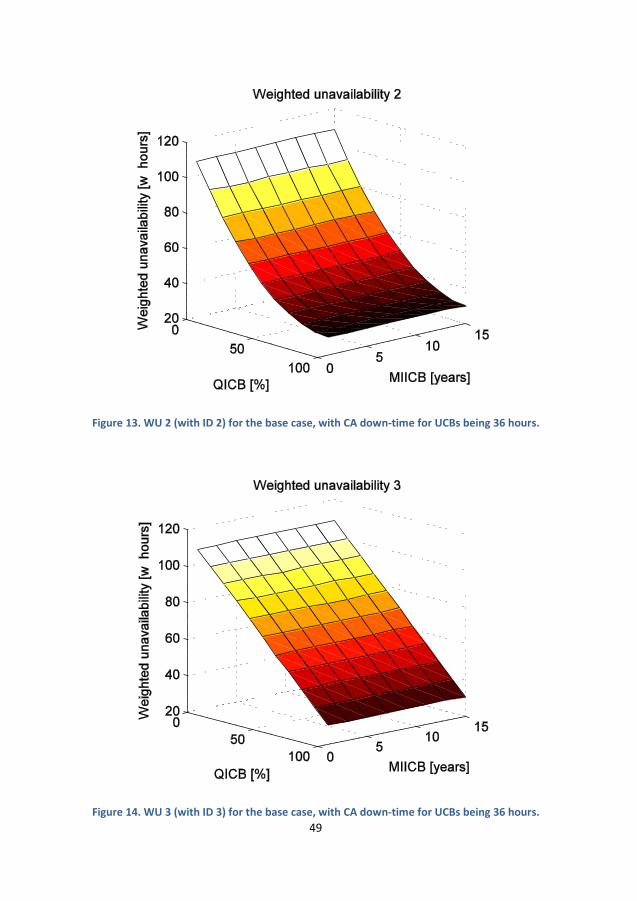
Figure 13. WU 2 (with ID 2) for the base case, with CA down-time for UCBs being 36 hours.
Figure 14. WU 3 (with ID 3) for the base case, with CA down-time for UCBs being 36 hours.

50
As previously mentioned in section 6.1, the only factor having a visible impact on the Figures 12-14
is the 36 hours CA time out of service for UCBs. The portion of the component population making
out the UCBs decreases as the QICB increases, hence the weighted unavailability of the
components decrease with an increasing QICB.
For these results, it becomes apparent what impact the different ways of taking component
importance into account makes. Figure 12 suggests that the impact of viewing up to 10 % of the
component population as important is sufficient, if the aim is to significantly decrease the
weighted time out of service by simply not performing the standard preventive maintenance
requiring 36 hours time out of service.
Figure 15 represents a similar simulation to the one represented in Figure 12, with the only
difference that QICB ranges from 0 to 0.1 instead of from 0 to 1.
Figure 15. WU 1 for the base case (QICB 0-10%), with CA down-time for UCBs being 36 hours.
This way zooming in on the steep increase in Figure 12, it is noticeable that the 3-4 % most critical
components stand for most of the decrease in WU.

51
6.1.2. CA time out of service for UCBs = 0 hours
Figure 16. WU 1 (with ID 1) for the base case, with CA down-time for UCBs being 0 hours.

52
Figure 17. WU 2 (with ID 2) for the base case, with CA down-time for UCBs being 0 hours.
Figure 18. WU 3 (with ID 3) for the base case, with CA down-time for UCBs being 0 hours.

53
With the CA time out of service for UCBs set to 0 hours, what the figures show is the WU from
corrective maintenance and scheduled replacements of CBs resulting from the various
combinations of QICB and MIICB. While WU in Figure 16 has seemingly no cohesive correlation (or
a very weak one) with the main variables, Figures 17 and 18 show that more frequent CAs and a
higher percentage of ICBs result in lower values for WU.
6.1.3. Results of single-point simulation
The results of a standard single-point simulation is displayed below, highlighting the inner
workings of the simulation. For a standard single-point simulation, the QICB is set to 10% and the
MIICB set to 5 years.
Time out of service
Total time and total weighted time out of service, due to corrective maintenance and scheduled
replacements of CBs are presented in Figures 19 and 20.
Figure 19. Total time out of service for the CB population.
0
500
1000
1500
2000
2500
1 4 7 10 13 16 19 22 25 28 31 34 37 40
Tim
e [
h]
Year
Total time out of service [h]

54
Figure 20. Total weighted (ID 1) time out of service for the CB population.
In Figure 20 the times out of service are weighted against the component importance (ID 1).
Number of measurements
The number of condition measurements for UCBs and ICBs respectively are shown in Figure 21.
Figure 21. Number of CAs for the CB population.
0,00
0,50
1,00
1,50
2,00
2,50
3,00
1 4 7 10 13 16 19 22 25 28 31 34 37 40
Tim
e [
we
igh
ted
ho
urs
]
Year
Total weighted time out of service [weight.h]
0
20
40
60
80
100
120
1 4 7 10 13 16 19 22 25 28 31 34 37 40
No
. of
me
asu
rem
en
ts
Year
No. of measurements
No. of CMs for UCBs
No. of CMs for ICBs

55
Number of replacements and repairs
The number of replacements due to failure and scheduling, as well as repairs due to failure.
Figure 22. Number of replacements and repairs for the CB population.
0
5
10
15
20
25
30
35
40
45
50
1 4 7 10 13 16 19 22 25 28 31 34 37 40
No
. of
mai
nte
nan
ce m
eas
ure
s
Year
No. of replacements & repairs
Sch. replacements
Fail. replacements
Fail. repairs
56
Age for scheduled replacement
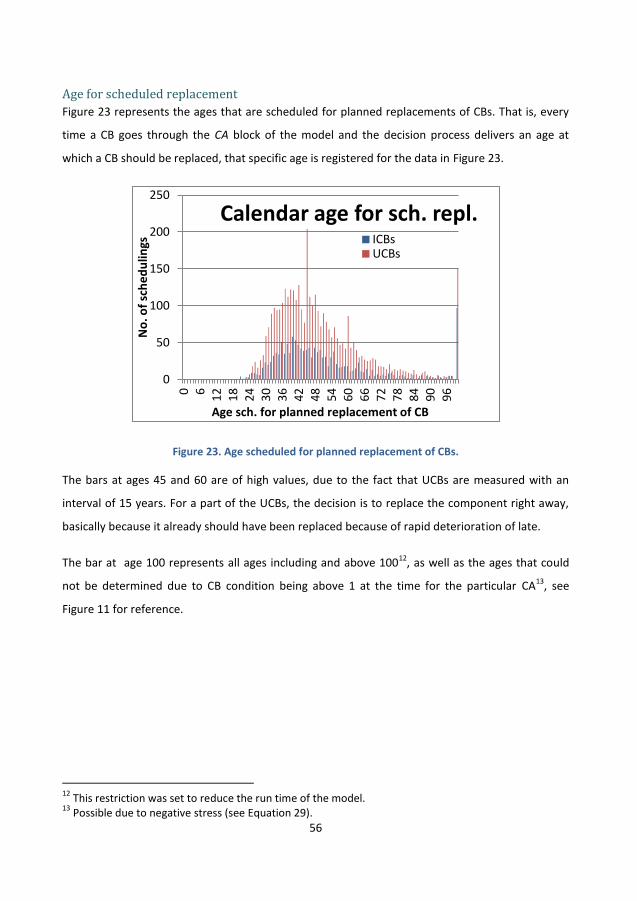
Figure 23 represents the ages that are scheduled for planned replacements of CBs. That is, every
time a CB goes through the CA block of the model and the decision process delivers an age at
which a CB should be replaced, that specific age is registered for the data in Figure 23.
Figure 23. Age scheduled for planned replacement of CBs.
The bars at ages 45 and 60 are of high values, due to the fact that UCBs are measured with an
interval of 15 years. For a part of the UCBs, the decision is to replace the component right away,
basically because it already should have been replaced because of rapid deterioration of late.
The bar at age 100 represents all ages including and above 10012, as well as the ages that could
not be determined due to CB condition being above 1 at the time for the particular CA13, see
Figure 11 for reference.
12
This restriction was set to reduce the run time of the model. 13
Possible due to negative stress (see Equation 29).
0
50
100
150
200
250 0
6
1
2
18
2
4
30
3
6
42
4
8
54
6
0
66
7
2
78
8
4
90
9
6
No
. of
sch
ed
ulin
gs
Age sch. for planned replacement of CB
Calendar age for sch. repl. ICBs
UCBs

57
Calendar age at replacement
Calendar age at the actual replacements of the CBs, as well as the numbers of replacements of
each category during the time horizon of the simulation are presented in Figures 24 and 25.
Figure 24. Age at replacement of CBs.
Figure 25. Number of replacements of CBs.
0
20
40
60
80
100
120
140 0
6
12
18
24
30
36
42
48
54
60
66
72
78
84
90
96
No
. of
CB
s
Calendar age at replacement
Calendar age at replacement
Fail. Repl.
Sch. Repl.
0
200
400
600
800
1000
1200
1400
1600
0 1 2 3 4 5 6 7 8 9 10
No
. of
CB
s
No. of replacements
No. of replacements
Fail. Repl.
Sch. Repl.

58
Average age at replacement
The average calendar and equivalent age respectively at replacement for each category of CBs.
Table 12. Average age at replacement for CB population.
CBs Calendar age Equivalent age
All CBs 40.7 1.38
Important CBs 43.3 1.45
Line CBs 41.4 1.39
Transformer CBs 41.8 1.40
Shunt reactor CBs 33.6 1.49
Capacitor CBs 39.7 1.40
Bus-coupler CBs 39.6 1.32
Other CBs 33.8 1.27
Average calendar age of CB population
The average calendar age of the CB population through the simulation is show-cased in Figure 26.
Figure 26. Average age of the CB population.
10
15
20
25
30
1 4 7 10 13 16 19 22 25 28 31 34 37 40
Cal
en
dar
age
Year
Average calendar age [years]
ICBs
All CBs

59
Five CBs’ conditions
The condition of 5 of the 1911 CBs in the population, throughout the simulation. The near-vertical
sections represent a replacement of the CB. The purpose of this plot is to show examples of how
CB condition may develop through the years.
Figure 27. The condition through the simulation of 5 breakers.
After replacement, breaker 1 and 3 clearly display the impact of the possibility of differing age
factors, as defined in Equation 2.
0
0,2
0,4
0,6
0,8
1
1,2
1 4 7 10 13 16 19 22 25 28 31 34 37 40
CB
co
nd
itio
n
Year
Five CBs' conditions
1
2
3
4
5

60
6.2. Results of sensitivity analysis The sensitivity analysis for this case study serves two purposes, first to verify that the model is
valid, and second to examine which factors are critical for a decision regarding introducing CAs in
a real component population. This is done solely for the results where the CA time out of service
for UCBs equals 0 hours, as any changes in the pattern are to be observed, and with this factor
equaling 36 hours, any patterns would be indistinguishable below the slope in Figures 12-15.
Several bases for comparison are used in this section, see Table 13. Among others, a previously
unmentioned part of the model output will be taken into account, namely the weighted ratio for
replacements due to failure versus scheduled replacements. A higher or lower value of this ratio is
not necessarily preferable or not, it does however provide a means of showing potential
differences between various cases in the sensitivity analysis. More information on how the ratio of
replacements is calculated is available in Appendix 3.
Table 13. Bases for comparison in the sensitivity analysis.
Model output Basis for
comparison
Weighted unavailability 1, 2, 3 (average)14 Value
Weighted unavailability 1, 2, 3 (3D-graph) Shape
Weighted replacement ratio15 1, 2, 3 (average) Value
Weighted replacement ratio 1, 2, 3 (3D-graph) Shape
Single-point simulation, QICB=10%, MIICB=5 yrs Various data16
In the following sections, the 3D-graphs have been assessed regarding the correlation they display
between the model variables and output. If a graph or the output data displays a distinguishable
(a-d) or distinct17 (A-D) correlation between the output data and the main variables, it is termed
correlation A through D, in accordance with Table 14. For example, Figure 18 in section 6.1.2
14
If QICB=[0,0.25,0.5,0.75,1] and MIICB=[1,3,6,9,12,15], then the WU average is the average of these 6*5=30 WU values 15
Replacements because of failure divided by scheduled replacements 16
Compare with figures 18 to 26 in section 6.1.3. 17
Subjectively assessed by the author

61
displays a distinguishable correlation a, having its lower values in the corner of large values for
QICB and small values for MIICB.
Table 14. An output 3D graph for either WU or WRR, is labeled according to which corner of the graph contains the lowest values.
Small
Large
QICB
QICB
Small MIICB C/c
A/a
Large MIICB D/d
B/b
Some 3D graphs are displayed directly in the following sections, marked in bold (A, a, B, …) in the
tables. For selected 3D-graphs from the sensitivity analysis that are not presented in the following
sections, marked with an x (AX, aX, BX, …) in the tables, see Appendix 4.
6.2.1. Base case for sensitivity analyses
Due to the limited time factor of the project, the output from the simulations in this sensitivity
analysis represent data averages from only 8 runs. To make these results comparable to the base
case of 1000 runs, the base case of 8 runs is presented in this section.
Run 0: The base case for the sensitivity analysis.
Table 15. Results of the base case adapted to the sensitivity analysis.
Run WU 1 WU 2 WU 3 WRR 1 WRR 2 WRR 3
0 30 - 31 - 31 - 0.62 - 0.62 a 0.62 a

62
Figure 28. WU 1 (with ID 1) for the sensitivity analysis base case.
Figure 29. WU 2 (with ID 2) for the sensitivity analysis base case.

63
Figure 30. WU 3 (with ID 3) for the sensitivity analysis base case.
The WU graphs in Figure 28-30 are after solely 8 runs not showing any correlation between either
QICB or MIICB and WU.

64
Figure 31. WRR 1 (with ID 1) for the sensitivity analysis base case.
Figure 32. WRR 2 (with ID 2) for the sensitivity analysis base case.

65
Figure 33. WRR 3 (with ID 3) for the sensitivity analysis base case.
The WRR graph in Figure 31 is not showing any correlation between the output and the main
variables. However, Figures 32 and 33 do show a distinguishable pattern, indicating a lower value
for lower values of MIICB and higher values of QICB (correlation a).
The output from a standard single-point simulation of the base case is the same as is displayed in
section 6.1.3.

66
6.2.2. Varying the time out of service
In this section the relationship between the times out of service for preventive and corrective
maintenance are varied.
Table 16. Altered values for times out of service.
Run Description Preventive
replacement
Corrective
repair
Corrective
replacement
0 24 h 24 h 48 h
1A No difference in down-times 48 h 48 h 48 h
1B Larger difference in down-times 24 h 48 h 96 h
Table 17. Results of the sensitivity analysis for case 1A and 1B.
Run WU 1 WU 2 WU 3 WRR 1 WRR 2 WRR 3
0 30 - 31 - 31 - 0.62 - 0.62 a 0.62 a
1A 39 - 39 - 39 - 1.76 - 1.78 a 1.78 a
1B 46 - 46 a 46 aX 0.22 - 0.22 a 0.22 a
The WU averages increase due to the time increases in both run 1A and run 1B, and have no
indication of the impact of the altered relationship between the factors. The WRR averages
however, clearly show that with larger times out of service for corrective maintenance, CBs are
replaced due to scheduling more often, and vice versa.

67
Figure 34. WU 2 for larger difference in down-times.
Figure 34 displays a correlation a.
Run 1A: Single-point simulation results
Calendar age at replacement
Figure 35. Age at replacement for no difference in down-times.
0
5
10
15
20
25
30
35
40
45
0
6
12
18
24
30
36
42
48
54
60
66
72
78
84
90
96
No
. of
CB
s
Calendar age at replacement
Calendar age at replacement
Fail. Repl.
Sch. Repl.

68
Figure 36. Number of replacements per CB for no difference in down-times.
The CBs run to failure or the age of 100, where they are automatically replaced in the simulation,
as displayed in Figure 35.
Average age at replacement
Table 18. Average age at replacement for no difference in down-times.
CBs Calendar age Equivalent age
All CBs 53.9 1.83
The average age of replacement is considerable higher than for the base case.
0
500
1000
1500
2000
0 1 2 3 4 5 6 7 8 9 10
No
. of
CB
s
No. of replacements
No. of replacements
Fail. Repl.
Sch. Repl.

69
Average calendar age of CB population
Figure 37. Average age of CB population for no difference in down-times.
The instability of the average calendar age of the CB population in this case is discussed in section
6.2.8. The instability is higher for the ICBs, as they only represent 10 % of the total CB population.
Five CBs’ conditions
Figure 38. Conditions of 5 CBs for no difference in down-times.
What Figure 38 clearly shows is that in a run to failure maintenance strategy the condition of a CB
can run very low before replacement.
20
25
30
35
40
1 4 7 10 13 16 19 22 25 28 31 34 37 40
Cal
en
dar
age
Year
Average calendar age [years]
ICBs
All CBs
-0,8
-0,6
-0,4
-0,2
0
0,2
0,4
0,6
0,8
1
1,2
1 4 7 10 13 16 19 22 25 28 31 34 37 40
CB
co
nd
itio
n
Year
Five CBs' conditions
1
2
3
4
5

70
Run 1B: Single-point simulation results
Calendar age at replacement
Figure 39. Age at replacement for larger difference in down-times.
Figure 40. Number of replacements per CB for larger difference in down-times.
In this run, as the Figures 39 and 40 display, the CBs are replaced much earlier than in the base
case.
0
50
100
150
200
250
300
350
400
450
0
6
12
18
24
30
36
42
48
54
60
66
72
78
84
90
96
No
. of
CB
s
Calendar age at replacement
Calendar age at replacement
Fail. Repl.
Sch. Repl.
0
500
1000
1500
2000
0 1 2 3 4 5 6 7 8 9 10
No
. of
CB
s
No. of replacements
No. of replacements
Fail. Repl.
Sch. Repl.

71
Average age at replacement
Table 19. Average age at replacement for larger difference in down-times.
CBs Calendar age Equivalent age
All CBs 29.4 1.00
The average age at replacement is lower than in the base case by more than a decade.
Average calendar age of CB population
Figure 41. Average age of CB population for larger difference in down-times.
As a result of early replacements, the average CB calendar age is lower than in the base case. The
oscillations for run 1B are not as considerable as the ones for run 1A, seen in Figure 37.
5
10
15
20
25
1 4 7 10 13 16 19 22 25 28 31 34 37 40
Cal
en
dar
age
Year
Average calendar age [years]
ICBs
All CBs

72
Five CBs’ conditions
Figure 42. Conditions of 5 CBs for larger difference in down-times.
Compared to run 1A or the base case, the CB conditions do not run as low before replacement in
run 1B.
0
0,2
0,4
0,6
0,8
1
1,2
1 4 7 10 13 16 19 22 25 28 31 34 37 40
CB
co
nd
itio
n
Year
Five CBs' conditions
1
2
3
4
5

73
6.2.3. Varying the stress factor
In this section the standard deviation of the randomly generated stress factor is altered.
Table 20. Altered stress factors.
Run Description Mean
value
Standard
deviation
0 0 0.03
2A No stress factor 0 0.00
2B Larger stress factor 0 0.06
Table 21. Results of the sensitivity analysis for case 2A and 2B.
Run WU 1 WU 2 WU 3 WRR 1 WRR 2 WRR 3
0 30 - 31 - 31 - 0.62 - 0.62 a 0.62 a
2A 31 - 31 - 31 a 0.63 - 0.60 d 0.60 d
2B 30 - 30 a 30 aX 0.63 - 0.63 A 0.64 A
Removing the stress factor, the WRR averages 2 and 3 display a correlation d, see Figure 43.
Meanwhile, an increased stress factor shows a clear correlation A, displayed in Figure 44.

74
Figure 43. WRR 3 for no stress factor.
Figure 44. WRR 3 for a larger stress factor.

75
Run 2A: Single-point simulation results
Five CBs’ conditions
Figure 45. Conditions of 5 CBs for no stress factor.
Without the impact of the stress factor, the condition deterioration follow a linear pattern.
Run 2B: Single-point simulation results
Five CBs’ conditions
Figure 46. Conditions of 5 CBs for larger stress factor.
0
0,2
0,4
0,6
0,8
1
1,2
1 4 7 10 13 16 19 22 25 28 31 34 37 40
CB
co
nd
itio
n
Year
Five CBs' conditions
1
2
3
4
5
0
0,2
0,4
0,6
0,8
1
1,2
1,4
1 4 7 10 13 16 19 22 25 28 31 34 37 40
CB
co
nd
itio
n
Year
Five CBs' conditions
1
2
3
4
5

76
An increased stress factor results in very unpredictable rates of deterioration for the CBs’
conditions. While breaker 3 in Figure 46 deteriorates rapidly before being replaced in the
beginning of the simulation, breaker 5 does not deteriorate at all over the course of the
simulation.

77
6.2.4. Varying the age factor
In this section the randomly generated age factor is altered.
Table 22. Altered age factor.
Run Description Mean
value
Standard
deviation
0 1 0.15
3A No difference in age factor 1 0.00
3B Increased range of age factor 1 0.30
Table 23. Results of the sensitivity analysis for cases 3A and 3B.
Run WU 1 WU 2 WU 3 WRR 1 WRR 2 WRR 3
0 30 - 31 - 31 - 0.62 - 0.62 a 0.62 a
3A 31 - 31 - 31 - 0.60 - 0.62 a 0.62 a
3B 31 - 31 a 31 a 0.62 - 0.63 a 0.63 AX
Run 3B provided clearer patterns in the correlations between the main variables and both WU 2
and 3 and WRR 3.

78
Figure 47. WU 3 for an increased range of age factor.
Run 3A: Single-point simulation results
Five CBs’ conditions
Figure 48. Conditions of 5 CBs for no difference in age factor.
0
0,2
0,4
0,6
0,8
1
1,2
1 4 7 10 13 16 19 22 25 28 31 34 37 40
CB
co
nd
itio
n
Year
Five CBs' conditions
1
2
3
4
5

79
In Figure 48, stress is the only factor separating the courses of deterioration for the CBs’
conditions. The stagnation or increase visible for CBs 4 and 5 are caused solely by negative stress,
as explained in section 4.2.2.
Run 3B: Single-point simulation results
Five CBs’ conditions
Figure 49. Conditions of 5 CBs for an increased range in age factor.
Breakers 1 and 5 represent two extremes in the respect of age factors in Figure 49. Where CB 1
appears to hardly deteriorate at all on average, the condition of CB 5 deteriorates with a relatively
steep slope as it ages.
0
0,2
0,4
0,6
0,8
1
1,2
1 4 7 10 13 16 19 22 25 28 31 34 37 40
CB
co
nd
itio
n
Year
Five CBs' conditions
1
2
3
4
5

80
6.2.5. Varying the hazard function
In this section the hazard function is altered in that the exponential factor is decreased and
increased.
Table 24. Altered hazard rate.
Run Description Exp. factor
0 0.0505
4A Decreased hazard rate 0.02525
4B Increased hazard rate 0.1010
Table 25. Results of the sensitivity analysis for cases 4A and 4B.
Run WU 1 WU 2 WU 3 WRR 1 WRR 2 WRR 3
0 30 - 31 - 31 - 0.62 - 0.62 a 0.62 a
4A 25 - 25 - 25 - 0.66 - 0.66 -X 0.66 -
4B 48 A 48 A 48 A 0.47 A 0.49 A 0.50 A
For the WU averages the value changes as one would expect with a more or less aggressive hazard
function, as it is an absolute measure. The WRR averages, a relative measure, however also display
a discrepancy from the results of the base case. An increased hazard rate results in a decrease in
the WRR average.
The shape of the 3D graphs clearly indicate a more distinct correlation A with a more aggressive
hazard function (Figure 50), and no correlation with a milder one (Figure 72).

81
Figure 50. WU 1 for an increased hazard rate.
Run 4A: Single-point simulation results
Calendar age at replacement
Figure 51. Age at replacement for a decreased hazard rate.
0
20
40
60
80
100
0
6
12
18
24
30
36
42
48
54
60
66
72
78
84
90
96
No
. of
CB
s
Calendar age at replacement
Calendar age at replacement
Fail. Repl.
Sch. Repl.

82
Figure 52. Number of replacements per CB for a decreased hazard rate.
The CBs are in general replaced at a far higher age in these results than in the base case.
Average age at replacement
Table 26. Average age at replacement for a decreased hazard rate.
CBs Calendar age Equivalent age
All CBs 62.6 2.12
The average age at replacement is significantly higher than in the base case.
0
200
400
600
800
1000
1200
1400
1600
0 1 2 3 4 5 6 7 8 9 10
No
. of
CB
s
No. of replacements
No. of replacements
Fail. Repl.
Sch. Repl.

83
Average calendar age of CB population
Figure 53. Average age of CB population for a decreased hazard rate.
The less aggressive hazard rate causes the average age of the CB population to oscillate
substantially. This effect is discussed further in section 6.2.8.
Five CBs’ conditions
Figure 54. Condition of 5 CBs for a decreased hazard rate.
With a less aggressive hazard rate, the CBs can deteriorate further than in the base case before
replacements are made.
25
30
35
40
45
1 3 5 7 9 11 13 15 17 19 21 23 25 27 29 31 33 35 37 39
Cal
en
dar
age
Year
Average calendar age [years]
ICBs
All CBs
-0,4
-0,2
0
0,2
0,4
0,6
0,8
1
1,2
1 4 7 10 13 16 19 22 25 28 31 34 37 40
CB
co
nd
itio
n
Year
Five CBs' conditions
1
2
3
4
5

84
Run 4B: Single-point simulation results
Calendar age at replacement
Figure 55. Age at replacement for an increased hazard rate.
Figure 56. Number of replacements per CB for an increased hazard rate.
The CBs are replaced at a considerably higher rate when the hazard function is more aggressive.
0
50
100
150
200
250
300
350
0
6
12
18
24
30
36
42
48
54
60
66
72
78
84
90
96
No
. of
CB
s
Calendar age at replacement
Calendar age at replacement
Fail. Repl.
Sch. Repl.
0
200
400
600
800
1000
1200
1400
0 1 2 3 4 5 6 7 8 9 10
No
. of
CB
s
No. of replacements
No. of replacements
Fail. Repl.
Sch. Repl.

85
Average age at replacement
Table 27. Average age at replacement for an increased hazard rate.
CBs Calendar age Equivalent age
All CBs 26.2 0.89
The higher replacement rate is reflected in the average age at replacement for the CBs.
Average calendar age of CB population
Figure 57. Average age of the CB population for an increased hazard rate.
Albeit stable, the average age of the CB population is low compared to the base case due to the
increased hazard rate.
5
10
15
20
25
1 4 7 10 13 16 19 22 25 28 31 34 37 40
Cal
en
dar
age
Year
Average calendar age [years]
ICBs
All CBs

86
Five CBs’ conditions
Figure 58. Condition of 5 CBs for an increased hazard rate.
The conditions of the CBs are not allowed to sink far before replacement, either corrective or
preventive.
0
0,2
0,4
0,6
0,8
1
1,2
1 4 7 10 13 16 19 22 25 28 31 34 37 40
CB
co
nd
itio
n
Year
Five CBs' conditions
1
2
3
4
5

87
6.2.6. Varying the measurement uncertainty
In this section the uncertainty of the CAs is altered.
Table 28. Altered CA uncertainty.
Run Description CA uncertainty
0 0.02
5A No CA uncertainty 0.00
5B Increased CA uncertainty 0.10
5C Increased CA uncertainty 0.20
Table29. Results of the sensitivity analysis of cases 5A, 5B and 5C.
Run WU 1 WU 2 WU 3 WRR 1 WRR 2 WRR 3
0 30 - 31 - 31 - 0.62 - 0.62 a 0.62 a
5A 30 - 31 - 31 - 0.61 aX 0.62 - 0.62 -
5B 30 - 31 - 31 - 0.60 - 0.61 AX 0.61 A
5C 31 d 31 - 32 - 0.57 - 0.57 A 0.58 A
For runs 5B and 5C the WRR averages 2 and 3 display a correlation A. However, it is difficult to
deduce any conclusions from these results, as the Wu averages remain unchanged. The exception
being WU 1 for run 5C, where correlation d can be distinguished, see Figure 59.

88
Figure 59. WU 1 for an increased CA uncertainty.
Run 5B: Single-point simulation results
Calendar age at replacement
Figure 60. Age at replacement for an increased CA uncertainty.
0
20
40
60
80
100
120
140
160
0
6
12
18
24
30
36
42
48
54
60
66
72
78
84
90
96
No
. of
CB
s
Calendar age at replacement
Calendar age at replacement
Fail. Repl.
Sch. Repl.

89
Figure 61. Number of replacements per CB for an increased CA uncertainty.
What the data in Figures 60 and 61 show is that the distribution of the replacements is the same
as in the base case, with the exception that the higher bars at every 15 years becomes higher the
higher the measurement uncertainty is.
Run 5C: Single-point simulation results
Calendar age at replacement
Figure 62. Age at replacement for an increased CA uncertainty.
0
500
1000
1500
2000
0 1 2 3 4 5 6 7 8 9 10
No
. of
CB
s
No. of replacements
No. of replacements
Fail. Repl.
Sch. Repl.
0
20
40
60
80
100
120
140
160
180
200
0
6
12
18
24
30
36
42
48
54
60
66
72
78
84
90
96
No
. of
CB
s
Calendar age at replacement
Calendar age at replacement
Fail. Repl.
Sch. Repl.

90
Figure 63. Number of replacements per CB for an increased CA uncertainty.
As explained earlier in this section, the graphs show a similar distribution to the base case, with a
higher concentration of CB replacements every 15 years. This is a direct measure of the
measurement uncertainty, as a larger amount of CBs is wrongly assumed to survive longer than it
will as well as wrongly deemed to be capable of going on longer than it is.
0
200
400
600
800
1000
1200
1400
1600
0 1 2 3 4 5 6 7 8 9 10
No
. of
CB
s
No. of replacements
No. of replacements
Fail. Repl.
Sch. Repl.

91
6.2.7. Varying the measurement uncertainty combined with an increased hazard
rate
Due to the difficulties determining any correlations solely from altering the uncertainty of the CA,
this section presents the alteration of CA uncertainty while keeping the hazard function as it is in
run 4B.
Table 30. Altered CA uncertainty in combination with an increased hazard rate.
Run Description CA uncertainty
4B Increased hazard rate 0.02
6A 4B + no CA uncertainty 0.00
6B 4B + increased CA uncertainty 0.10
6C 4B + increased CA uncertainty 0.20
Table 31. Results of the sensitivity analysis for cases 6A, 6B and 6C.
Run WU 1 WU 2 WU 3 WRR 1 WRR 2 WRR 3
4B 48 A 48 A 48 A 0.47 A 0.49 A 0.50 A
6A 48 A 48 A 48 A 0.47 A 0.49 A 0.50 A
6B 48 aX 49 A 49 A 0.46 A 0.49 A 0.50 A
6C 50 a 50 a 51 a 0.44 A 0.48 A 0.51 A
In the light of these simulations it would seem that an increased CA uncertainty weakens the
correlation A, to the point where the reverse might appear in the form of correlation d18.
18
Run 5C

92
Figure 64. WU 1 for an increased CA uncertainty and an increased hazard rate.
Run 6C: Single-point simulation results
Calendar age at replacement
Figure 65. Age at replacement for an increased CA uncertainty and an increased hazard rate.
0
50
100
150
200
250
300
350
400
450
0
6
12
18
2
4
30
3
6
42
4
8
54
6
0
66
7
2
78
8
4
90
9
6
No
. of
CB
s
Calendar age at replacement
Calendar age at replacement
Fail. Repl.
Sch. Repl.

93
Figure 66. Number of replacements per CB for an increased CA uncertainty and an increased hazard rate.
The same conclusion as in section 6.2.6 can be reached from comparing Figures 65 and 66 with
corresponding Figures 62 and 63, where only the hazard function was altered. A considerably
higher amount of CBs is replaced every 15 years due to CAs being far off the mark.
Five CBs’ conditions
Figure 67. Conditions of 5 CBs for an increased CA uncertainty and an increased hazard rate.
Breaker 3 in Figure 67 is very likely being replaced too early, and breaker 5 too late (first
replacement), possibly due to failure which could have been avoided had it been replaced earlier,
compare with Figure 58. This clearly shows the effects of poor measurement accuracy.
0
200
400
600
800
1000
1200
1400
0 1 2 3 4 5 6 7 8 9 10
No
. of
CB
s
No. of replacements
No. of replacements
Fail. Repl.
Sch. Repl.
0
0,2
0,4
0,6
0,8
1
1,2
1 4 7 10 13 16 19 22 25 28 31 34 37 40
CB
co
nd
itio
n
Year
Five CBs' conditions
1
2
3
4
5

94
6.2.8. Comments
Transient effects
For runs 1A and 4A (Figures 37 and 53) as well as the result in the base case (Figure 26) it can be
observed, through the single-point simulation graphs over average calendar age, that they are
affected by a transient effect causing oscillations in calendar age. The same effect also appears in
the graphs for time out of service and the number of maintenance measures performed. The
transient effects are caused by the simulations not having had enough time to settle after a
change has been introduced.
In the base case it merely concerns a change in the average calendar age over the population by a
couple of years. However, in run 1A it concerns a change of 5 years in average age, and in the case
of run 4A the change is as much as 12 years. These transients may significantly affect the results of
these runs.
Attempts to avoid this problem, that at first was present also for the base case results, have been
made in two parts. In the first simulations for the base case, the starting age of the CBs were
uniformly distributed between 0 and 30, creating an average age of 15. At the start of that
simulation, the average age rose to about 25, overshooting the eventually settled average age of
21 by 4 years, before sinking once more.
The first part of attempting to solve the problem, was to start a simulation for the base case as
described above, run it for several hundred years, and then take out the ages, age factors and
conditions19 of all CBs, henceforth using them as the new starting properties for the CB
population.
The approach mentioned above did significantly decrease the settling time of the oscillations,
killing it off after the first half period of the oscillations. The overshoot was nevertheless still as
prominent, even though the simulation started at the “right” average age. This is caused by the
fact that not all CBs have been measured for the first time until year 15 of the simulation, and may
because of that go for up to 15 years having a too high age than what would be optimal. To
19
The age factors and conditions were also included, as the problem is caused by between themselves unmatching ages, age factors and conditions as well as a too high or low starting average age of the CB population.

95
absolve the model of this, the first 30 years of the simulation, as mentioned in section 5.1 on the
model settings, were not recorded, this way allowing the oscillations to settle.
Yet, as proved, they still occur. For most single-point simulations of the cases in the sensitivity
analysis, the transient effects seem non-existent. However, as previously mentioned, it is
amplified for some cases. The common factor between runs 1A and 4A is a significantly higher
average age of the CB population after settling20. In run 1A it is due to nearly all CBs running to
failure, and in run 4A it is due to a decreased failure rate.
Drastically increasing the times out of service
At a number of trial simulations not presented in this thesis report, the times out of service for
corrective maintenance were increased by a factor 5 and a factor 10. For the latter case, the
results showed a clear correlation D. for the down-times being multiplied by 5, the results showed
a clear dip in the center of the WU 3D graph. After studying the results of the single-point
simulations, it was apparent that the simulation no longer represented any realistic scenario. For
instance, in a single-point simulation with the QICB at 10 %, nearly all UCBs were immediately
replaced after the first CA at age 15. In such a reality, the basic settings, such as not measuring CBs
until the age of 15, are unrealistic.
Thus it can be deduced that the model is not valid for very high values of the times out of service
for corrective maintenance in comparison to the value for scheduled replacements21.
Varying the equivalent age
At an earlier stage additional simulations were performed where the relationship between
calendar age and number of operations was altered. This did however not have any relevant
impact on the results. The sole visible change was that shunt reactor CBs and other types of CBs
with a high number of annual operations were replaced at an earlier or later calendar age
compared to what they are in the base case in relation to other types of CBs.
20
These values are not yet settled at the end of runs 1A and 4A. This can though be intuitively understood when viewing the preconditions for these simulations. 21
Kept at 24h.

96

97
7. CLOSURE
7.1. Discussion
Prevailing time for periodic preventive maintenance
The main results show that the 36 h it takes to perform a condition measurement for a UCB, has
the significantly highest impact on the weighted unavailability of the component population.
Looking at the edge of the graphs in Figures 12 to 14, where the QICB equals 100%, it logically
should coincide with the same edge in the graphs in Figures 16 to 18, that way showing a slight
impact of varying the MIICB. However, this effect is practically non-existent in comparison with
varying the QICB.
The effects of using component importance
The results in section 6.1.1 also show the effect of applying different component importance
values and rankings. The importance indices (ID 1) give a clear indication of how large a
percentage of the CB population should be viewed as important22 for significant savings in
component time out of service for preventive maintenance. The results from using the importance
ranking (ID 2), or no importance weighting (ID 3), are not presenting the same tangible limit.
For the results in section 6.1.2, where the CA time out of service for UCBs is set to 0, the effects of
the importance indices are the opposite. The cases where no importance weighting is applied are
the ones that in all cases are the quickest to show any patterns in the correlation between the
main variables and the weighted unavailability, followed by the cases with importance ranking.
The WU 3D graphs output from the simulation using the importance indices, are highly influenced
by the randomness of the simulations, seeing as only 3-4%23 of the CBs have the significantly
largest impact on the results. This way, the results reflect a CB population severely diminished,
requiring a high amount of iterations before any statistically verified results can be obtained.
Critical factors for decision-making regarding condition measurements
In examining the results of the sensitivity analysis, there are some key observations to be made.
22
In this case for the specific grid investigated in [6]. 23
See section 6.1.1, figures 11 and 14.

98
Altering the factors affecting the development of the CB condition, the age factor and the stress
factor, shows that an increased randomness in the behavior of the CB condition more quickly24
justifies the use of CAs as a means of obtaining a lower unavailability for the system’s
components. In the same way, an increased failure rate also motivates the use of condition
measurements. The shorter the intervals between measurements, and the larger the percentage
of CBs receiving this treatment, the more is to be gained in terms of lowered component
unavailability.
It has been showed to be more difficult to motivate a maintenance strategy including condition
measurements for cases with decreased failure rates, as well as for cases where the uncertainty of
the condition measurements is high.
The fact that the condition measurement uncertainty is a sensitive factor when deciding whether
to implement a maintenance strategy including CAs or not, puts a large focus on the availability of
reliable measurement methods. How accurately does the measurement reflect the measured
parameter? How does the measured parameter reflect on the CB’s condition, and how large a
percentage of the CB failure modes could measurements of the parameter anticipate? These are
valid questions when considering condition based maintenance strategies.
Model validity
While the model does not appear to be sensitive to large changes in the factors mentioned above,
changing the times out of service for corrective maintenance does have a limit for model validity,
as discussed in section 6.2.8. Increasing these down-times for corrective maintenance in relation
to down-times for preventive replacements, does nevertheless indicate a correlation between
frequent intervals of CAs, high percentages of important CBs and low values of WU.
Expectations and unforeseen findings
A great part of the results discussed above on the benefit of condition assessment could be
anticipated beforehand. There were however an amount of unexpected findings along the way,
discussed below in three parts.
24
In terms of number of iterations for the simulations, that is the randomness in the results are decreased.

99
The impact of the time for the periodic preventive maintenance of the UCBs, that is the
CA time out of service for these CBs, was considerably higher than anticipated. See
earlier discussion in this section.
An important factor that could have improved the results of this thesis, had it been
anticipated, is the number of iterations in running the simulations that are required for a
desirable statistical reliability. As listed in Appendix 2, the base case results are run with
1000 iterations, which is still too low for Figure 16 to show any clear result. For the
sensitivity analysis only 8 iterations were used per case, which is a very low number of
iterations, due to the overall time limit of this project. Refer to Appendix 5 for the
correlation between number of iterations and reduced variance of results.
Throughout the work on this thesis it has been obvious that any changes in maintenance
strategy, be it in this case the interval between condition measurements, the quota of
important circuit breakers or any other factors affecting the simulations, create transient
effects in the component population. The transient effects, affecting the mean age of the
component population and so the amount of corrective maintenance required due to an
increase or decrease in overall risk of failure, have period times spanning several
decades, and can take more than a century before showing any sign of settling. For a
power grid owner, this could have a deep financial impact, that needs to be anticipated
and taken into account when any decisions regarding maintenance strategy are to be
made.

100
7.2. Conclusions The recommendations from this project consist of a number of points that need to be investigated
by the individual grid operators for the results from this study to be fully applicable. Initially, the
most critical components (or component criticality for all the system components) need to be
identified. Secondly, methods of condition measurements and their accuracy in reflecting the
component condition need to be examined. In addition to these points it would also be logical to
investigate the feasibility of excluding components from all regular off-line preventive
maintenance actions.
In summary, the following conclusions were reached from the results of this thesis project:
Replacing the periodic off-line preventive maintenance with on-line condition
measurements for the most critical circuit breakers in a power transmission system,
significantly diminishes the weighted overall down-time for all circuit breakers in the
system.
Disregarding the down-time for the periodic preventive maintenance in the total
weighted unavailability of the circuit breakers, shows that it is most preferable to use
frequent intervals for condition measurements for a large part of the circuit breaker
population, regardless of whether importance indices, importance ranking, or no
importance weighting is applied.
A maintenance strategy based on condition measurements is best motivated in cases
where the randomness of circuit breaker condition deterioration is high, the failure rate
is high, condition measurements have low uncertainty, or the down-times for corrective
maintenance actions are high in relation to preventive maintenance actions.
A maintenance strategy based on condition measurements is less motivated or
unmotivated in cases where the randomness of circuit breaker condition deterioration is
low, the failure rate is low, or condition measurements have high uncertainty.
Severe transient effects in overall average age of the component population may appear
in response to any changes in maintenance strategy (or the lack of it). These transients
can lead to peaks in failures (and so costs for corrective maintenance), having a harsh
impact for power system owners.

101
7.3. Future work
Refining the model
The model in this thesis work is rough in several aspects. There are numerous improvements that
can be made, and factors to take into account. A few of them are listed below.
The decision process in the model could be replaced by more optimal ways of handling
the measurement data
More alternative failure mechanisms for circuit breakers could be explored, for instance
in the way they are investigated in [11], where several more corrective maintenance
actions are applied.
The positive effect of the periodic preventive maintenance, where actions such as
lubricating and exercising of the circuit breakers take place, should be taken into
account. There may still be a need of some sort of off-line maintenance being performed
during the circuit breakers’ lifetime.
Extending the simulations
For a future extension of the model, it would be of interest to run the simulations through more
iterations to reduce the noise in the resulting data. It would also be relevant to extend the start-up
period of the simulations or by other means avoid the impact on the results by the transient
effects.
The particular case study performed in this thesis work focuses on the circuit breaker population
of a power transmission system. It could be developed to include other types of components, such
as transformers, disconnectors, over-head lines and cables, as well as compensating equipment.
Cost aspects
For distribution grids, where the N-1 criterion is not applied as rigorously as in transmission grids,
the cost aspect of components being out of service might weigh heavier than the time aspect.
Looking at the cost aspect of different maintenance strategies, down-time is only one factor in
anticipating the consequence of component failure. Moreover, time-wise, on-line measurements
are free (as they are performed on-line) which in all likelihood is not correct cost-wise.

102
Impact of transient effects
The transient effect observed in this thesis has a veritably relevant equivalent in real life
transmission and distribution grids. The impact of an overall ageing component population, due to
a low level of re-investments, may very well result in peaks in component failure, having a
considerable impact on costs of corrective maintenance and man-power required. It would be
beneficial for any grid owner to be aware of the possibility of these peaks, that if anticipated in
time, perhaps could be avoided completely.
A study of this sort could also include investigations of when the peaks in the transients would be
likely to occur for the various component populations, as the respective component types
undoubtedly have differing life expectancies.

103
REFERENCES
[1] P. Hilber, “Maintenance Optimization for Power Distribution Systems”, Doctoral Thesis, KTH,
2008.
[2] Cigré Working Group B3.12, “462: Obtaining Value from On-Line Substation Condition
Monitoring”, 2011.
[3] Svenska Kraftnät, “TR12-09: Riktlinjer för underhåll av stationer”, Technical guideline, 2009
[4] Cigré Working Group 13.08, ”165: Life Management of Circuit-Breakers”, 2000.
[5] Cigré Working Group A3.06, “510: Final Report of the 2004 – 2007 International Enquiry on
Reliability of High Voltage Equipment: Part 2 – Reliability of High Voltage SF6 Circuit
Breakers”, 2012.
[6] J. Setréus, “Identifying critical components for system reliability in power transmission
systems”, Doctoral Thesis, KTH, 2011.
[7] ABB, “Produktmanual 1HSB445416-31 sv1 – Frånskiljande brytare”, 2009.
[8] IEC 62271-100 International Standard, “High-voltage switchgear and controlgear – Part 100:
Alternating-current circuit-breakers”, 2nd Ed., 2008.
[9] T. M. Lindquist, Svenska Kraftnät, Stockholm, 21 May 2013.
[10] T. M. Lindquist, Svenska Kraftnät, Stockholm, 11 March 2013.
[11] T. M. Lindquist, L. Bertling and R. Eriksson, “Circuit breaker failure data and reliability
modelling”, IET Generation, Transmission & Distribution, 2008.
[12] B. W. Lindgren, Statistical Theory, The Macmillan Company, 2nd Ed. 1968.

104

105
APPENDIX 1: Derivation of the hazard function
In this appendix, it is presented how the hazard function (Equation 27) is derived.
Eq. 27
The data in Table 32 and Figure 68, obtained from [5]25, gives an indication of how the risk of
failure26 depends on the age of a CB.
Table 32. Failure frequency per CB year [5].
Age Failure frequency (per
CB year)
Distribution of
population
25 0,0094 8 %
20 0,0062 13 %
15 0,0042 21 %
10 0,0044 22 %
5 0,004 21 %
0 0,0018 15 %
25
Table 2-109, All countries, Live tank 26
Major failure – defined by [5] as “Major failure modes prevent circuit breakers from performing their basic functions”.

106
Figure 68. Plotted failure rate per CB year.
The exponential curve fitted against the weighted data points give the risk function based on CB
calendar age.
Eq. 28
To obtain a hazard function based on CB condition, the following correlations are applied.
Eq. 29
Eq. 30
27
28 Eq. 31
Eq. 32
Discrepancy
The discrepancy caused by the approximation in Equation 30 has a limited impact. For instance, a
CB with 45 operations per year (the average for the CB population) has at the age of 25 performed
1125 operations:
27 Approximation, the number of operations are not included. 28
Estimated calendar age – as the calendar age has no causal dependence of the CB condition
y = 0,0024e0,0505x
0
0,001
0,002
0,003
0,004
0,005
0,006
0,007
0,008
0,009
0,01
0 10 20 30
Failu
res
pe
r C
B y
ear
Age

107
Approximate equivalent age:
Exact equivalent age:
Discrepancy:

108

109
APPENDIX 2: Settings for QICB, MIICB and number of iterations for each
simulation
Table 33. Settings for each simulation presented in Chapter 6.
Run QICB MIICB No. of iterations
Base case
(6.1.1)
0:0.1:1 1:2:15 5
Base case
(Fig 14)
0:0.01:0.1 1:2:15 5
Base case
(6.1.2)
0:0.2:1 [1,3,6,9,12,15] 1000
0 0:0.2:1 [1,3,6,9,12,15] 8
1A 0:0.25:1 [1,3,6,9,12,15] 8
1B 0:0.25:1 [1,3,6,9,12,15] 8
2A 0:0.25:1 [1,3,6,9,12,15] 8
2B 0:0.25:1 [1,3,6,9,12,15] 8
3A 0:0.25:1 [1,3,6,9,12,15] 8
3B 0:0.25:1 [1,3,6,9,12,15] 8
4A 0:0.25:1 [1,3,6,9,12,15] 8
4B 0:0.25:1 [1,3,6,9,12,15] 8
5A 0:0.25:1 [1,3,6,9,12,15] 8
5B 0:0.25:1 [1,3,6,9,12,15] 8
5C 0:0.25:1 [1,3,6,9,12,15] 8
6A 0:0.25:1 [1,3,6,9,12,15] 8
6B 0:0.25:1 [1,3,6,9,12,15] 8
6C 0:0.25:1 [1,3,6,9,12,15] 8

110
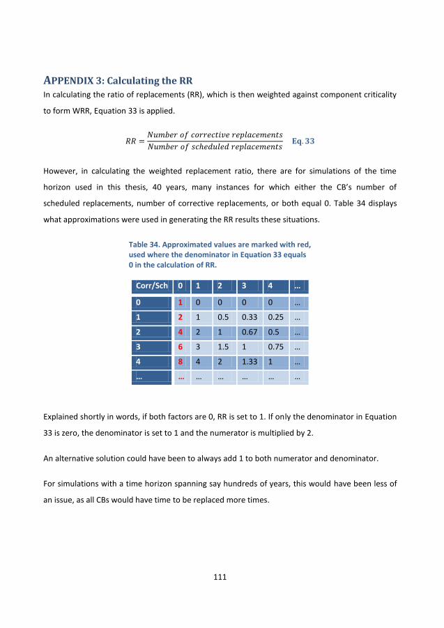
111
APPENDIX 3: Calculating the RR
In calculating the ratio of replacements (RR), which is then weighted against component criticality
to form WRR, Equation 33 is applied.
However, in calculating the weighted replacement ratio, there are for simulations of the time
horizon used in this thesis, 40 years, many instances for which either the CB’s number of
scheduled replacements, number of corrective replacements, or both equal 0. Table 34 displays
what approximations were used in generating the RR results these situations.
Table 34. Approximated values are marked with red, used where the denominator in Equation 33 equals 0 in the calculation of RR.
Corr/Sch 0 1 2 3 4 …
0 1 0 0 0 0 …
1 2 1 0.5 0.33 0.25 …
2 4 2 1 0.67 0.5 …
3 6 3 1.5 1 0.75 …
4 8 4 2 1.33 1 …
… … … … … … …
Explained shortly in words, if both factors are 0, RR is set to 1. If only the denominator in Equation
33 is zero, the denominator is set to 1 and the numerator is multiplied by 2.
An alternative solution could have been to always add 1 to both numerator and denominator.
For simulations with a time horizon spanning say hundreds of years, this would have been less of
an issue, as all CBs would have time to be replaced more times.

112

113
APPENDIX 4: Select graphs from the sensitivity analysis
Run 1B
Figure 69. WU 3 for a large difference in down-times.
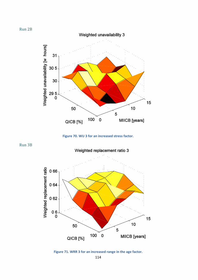
114
Run 2B
Figure 70. WU 3 for an increased stress factor.
Run 3B
Figure 71. WRR 3 for an increased range in the age factor.

115
Run 4A
Figure 72. WRR 2 for a decreased hazard rate.
Run 5A
Figure 73. WRR 1 for no CA uncertainty.

116
Run 5B
Figure 74. WRR 2 for an increased CA uncertainty.
Run 6B
Figure 75. WU 1 for an increased CA uncertainty and an increased hazard rate.

117
APPENDIX 5: Number of iterations versus variance reduction
The results of this thesis project has clearly shown that a higher number of simulation iterations
produces more smooth29 3D graphs. This is especially seen to be the case for the WU 1 (see
Figures 16 and 28), where a few number of components affect the largest part of the output data.
This process is explained in mathematical statistics as “The asymptotic distribution of the mean of
a random sample is (according to the central limit theorem) normal with mean and variance
. That is, the limiting distribution of
as becomes infinite, is standard normal – independent of the population distribution as long as
the latter has second moments.” [12]. See Table 35 for an idea of how quickly the number of
iterations necessary to produce results with reduced variance grows.
Table 35. The variance amongst the resulting data decreases with an increasing number of independent iterations.
No. of
iterations
Variance No. of
iterations
Variance
1 1.00 100 0.10
5 0.45 500 0.04
8 0.35 1 000 0.03
20 0.22 10 000 0.01
50 0.14 100 000 0.003
29
A lower variance among the data
Eq. 33