laboratory experiences and 3d measurements with … · laboratory experiences and 3d measurements...

Laboratory experiences and

3D measurements with AL5A Robot Arm

A thesis presented to

the Department of Mechanical Engineering

Politecnico di Milano

by

Ahmet Erhan DINC 749688

Fatih PEHLIVAN 749464

July 2011

APPROVED BY

Ing. Zappa EMANUELE__________________________________

i

Abstract

Lynxmotion AL5A robot arm is assembled in the measurement laboratory according to

instructions of the producer. After mechanical assembly, SSC-32 electric-control unit

connections are done in a suitable way. By using a serial-USB cable, RIOS computer program

can be run in order to set up configurations and calibrations. Through mounting GP2D12

sensor to the gripper and to the SSC-32 analog input pins, 3D scan images are taken

automatically. Besides, with the robot arm, basic experiments are created such as taking the

dices and carrying of them to the another place through steps and sequences. As a final step of

thesis, the possibility of interface with Labview program is investigated. For this purpose,

simple codes are written in Labview environment according to inverse kinematics and

Denavit-Hertanberg parameters of the robot arm.

ii

Table of Contents

Abstract ...................................................................................................................................... i

Table of Contents ..................................................................................................................... ii

List of Figures .......................................................................................................................... iv

List of Tables .......................................................................................................................... viii

1. Introduction ....................................................................................................................... 1

1.1. History of robotics ....................................................................................................... 1

1.2. Types and classification of robots ............................................................................... 4

2. AL5A robot arm ................................................................................................................ 6

2.1. Features of the AL5A robot arm .................................................................................. 6

2.1.1. The Mechanics of the robot .................................................................................. 6

2.1.2. The Electrical system of the robot ........................................................................ 6

2.1.3. Arm control options ............................................................................................. 7

2.2. Assembly of the AL5A robot arm ............................................................................... 9

2.2.1. Assembly of the base: .......................................................................................... 9

2.2.2. Assembly of the arm .......................................................................................... 16

2.2.3. Assembly for heavy-duty motion ....................................................................... 27

3. Controlling of AL5A with lynxmotion RIOS ............................................................... 30

3.1. Configuration of the SSC-32 card ............................................................................. 30

3.2. Configuration of the gravity compensate .................................................................. 35

3.3. The 'Moves / Motions' module .................................................................................. 36

3.3.1. Storing data of the robot position ....................................................................... 37

3.3.2. Storing data of the features ................................................................................. 39

3.4. The 'Play' module ...................................................................................................... 41

3.4.1. Play features ....................................................................................................... 41

3.4.2. Output options .................................................................................................... 42

3.4.3. Sequence list ....................................................................................................... 43

3.5. Analog inputs ............................................................................................................. 46

4. Basic experiments ............................................................................................................ 48

4.1. Project ........................................................................................................................ 48

4.1.1. Sequence 1 .......................................................................................................... 48

4.1.2. Sequence 2 .......................................................................................................... 51

iii

4.1.3. Sequence 3 .......................................................................................................... 54

4.2. Play of the project ...................................................................................................... 57

4.2.1. Example of “For” loops ...................................................................................... 57

4.2.2. Example of “If – Break” structure ...................................................................... 59

4.2.3. Example of “While-Do” structure ...................................................................... 61

5. Infrared distance sensors ............................................................................................... 63

5.1. Features, applications and maximum ratings ............................................................ 64

5.2. Outline dimensions .................................................................................................... 65

5.3. Electro-optical characteristics .................................................................................... 66

5.4. Internal block diagram and time chart of GP2D12 .................................................... 66

5.5. Analog output voltage graphics ................................................................................. 67

6. 3D scanning experiments ................................................................................................ 69

7. Controlling of the arm with Labview interface ............................................................ 76

7.1. Controlling of the D.O.F.s seperately ........................................................................ 76

7.2. Robot identification in Labview ................................................................................ 77

7.2.1. Introduction to kinematic analysis for Labview ................................................. 77

7.2.2. Denavit – Hertanberg (DH) parameters ............................................................. 78

7.2.3. Inverse kinematic frame and DH parameters of the AL5A robot arm ............... 80

8. Conclusion and future aspects ....................................................................................... 82

9. References ........................................................................................................................ 83

iv

List of Figures

Figure 1: Types of the robots ..................................................................................................... 4

Figure 2 : The overview of the robot electrical system .............................................................. 7

Figure 3 : Base bearings attachments ......................................................................................... 9

Figure 4 : Base ............................................................................................................................ 9

Figure 5 : Base mounting ........................................................................................................... 9

Figure 6 : Base bearings ........................................................................................................... 10

Figure 7 : Base servomotor ...................................................................................................... 10

Figure 8 : Base servo mounting ................................................................................................ 10

Figure 9 : Connection of the brackets ...................................................................................... 11

Figure 10 : Base lubrication ..................................................................................................... 11

Figure 11 : Front view of the base ............................................................................................ 11

Figure 12 : Cable of the base servomotor ................................................................................ 12

Figure 13 : Hex spacer connection ........................................................................................... 12

Figure 14 : Bracket of hex spacers ........................................................................................... 12

Figure 15 : Wiring connection ................................................................................................. 13

Figure 16 : Battery wire connection ......................................................................................... 13

Figure 17 : Mounting of SSC-32 to the hex spacer .................................................................. 13

Figure 18 : Power supply connections to the SSC-32 (Left side) ............................................ 14

Figure 19 : Power supply connections to the SSC-32 (Right Side) ......................................... 14

Figure 20 : Attaching of the base to the hex spacer and SSC-32 ............................................. 14

Figure 21 : Base servomotor connection to the SSC-32 .......................................................... 15

Figure 22 : Initial testing on Lynxmotion Terminal ................................................................. 15

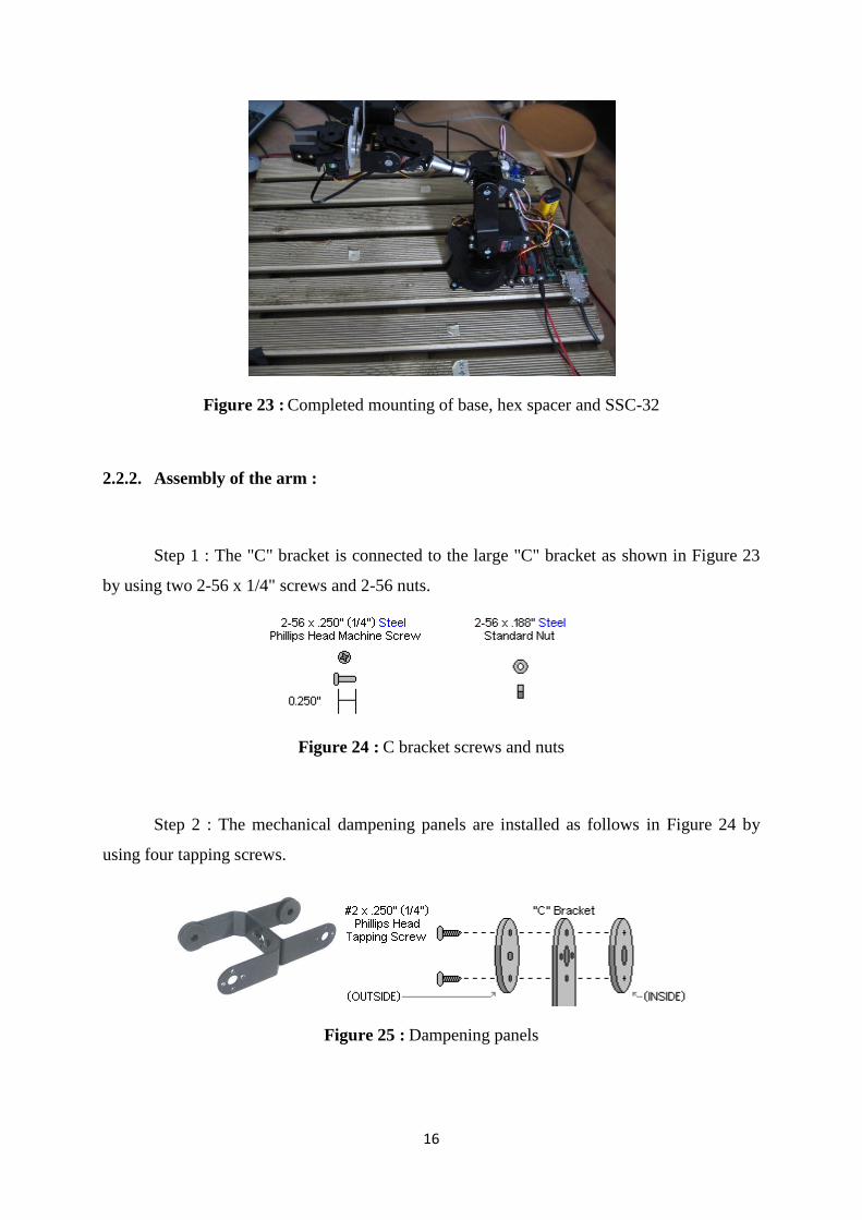
Figure 23 : Completed mounting of base, hex spacer and SSC-32 .......................................... 16

Figure 24 : C bracket screws and nuts ...................................................................................... 16

Figure 25 : Dampening panels.................................................................................................. 16

Figure 26 : Multi – purpose bracket for arm ............................................................................ 17

Figure 27 : Mounting of the arm to the bracket ....................................................................... 17

Figure 28 : Typical mega size of a servomotor ........................................................................ 18

Figure 29 : Mounting of HS-755HB to the arm bracket .......................................................... 18

Figure 30 : Mounting of the tubes ............................................................................................ 18

Figure 31 : Attaching of the tubes to the hubs ......................................................................... 19

v

Figure 32 : Attaching of the tubes to the multi-purpose brackets ............................................ 19

Figure 33 : Head screw connection to the multi purpose bracket of the tubes ........................ 19

Figure 34 : Output horn of servomotor .................................................................................... 20

Figure 35 : Attaching of HS-645HB to the bracket ................................................................. 20

Figure 36 : Gripper connector .................................................................................................. 21

Figure 37 : Mounting gripper connector to the C bracket ........................................................ 21

Figure 38 : Attaching of HS-422 to the C bracket ................................................................... 22

Figure 39 : Little grip ............................................................................................................... 22

Figure 40 : Extender cables for 6th servo................................................................................. 22

Figure 41 : Cable arrangement of wrist servo .......................................................................... 23

Figure 42 : Cable arrangement of the arm ................................................................................ 23

Figure 43 : Lynxterm channel slider ........................................................................................ 24

Figure 44 : Lynxterm All=1500 ............................................................................................... 24

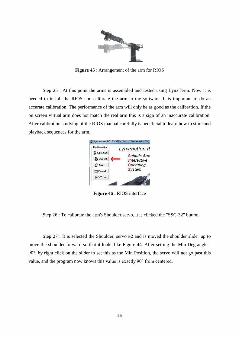
Figure 45 : Arrangement of the arm for RIOS ......................................................................... 25

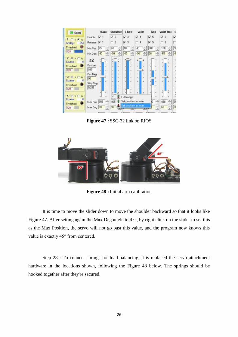
Figure 46 : RIOS interface ....................................................................................................... 25

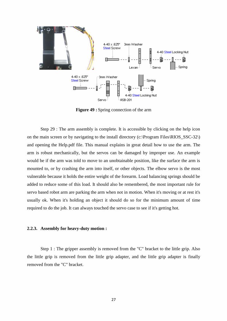
Figure 47 : SSC-32 link on RIOS ............................................................................................. 26

Figure 48 : Initial arm calibration ............................................................................................ 26

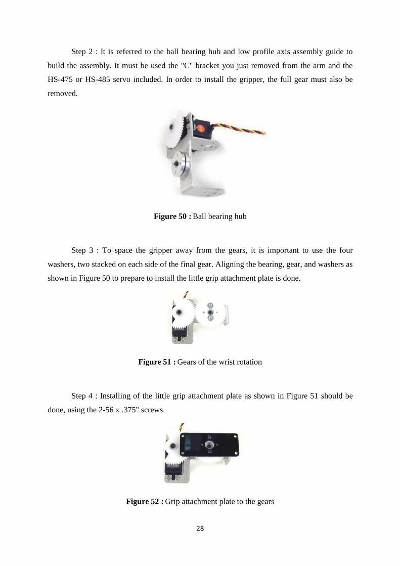
Figure 49 : Spring connection of the arm ................................................................................. 27

Figure 50 : Ball bearing hub ..................................................................................................... 28

Figure 51 : Gears of the wrist rotation ..................................................................................... 28

Figure 52 : Grip attachment plate to the gears ......................................................................... 28

Figure 53 : Attaching of the grip to the hexan ......................................................................... 29

Figure 54 : Panel of the program .............................................................................................. 30

Figure 55 : Adjusting Min and Max positions ......................................................................... 32

Figure 56 : Gravity compansate ............................................................................................... 35

Figure 57 : Moves part by mouse ............................................................................................. 36

Figure 58 : Panel of x,y and z motion ...................................................................................... 36

Figure 59 : Panel of distance, y and base angle motion ........................................................... 37

Figure 60 : Panel of joint motion ............................................................................................. 37

Figure 61 : Storing data interface ............................................................................................. 37

Figure 62 : Input preferences ................................................................................................... 40

Figure 63 : Play module of RIOS ............................................................................................. 41

Figure 64 : Output options ....................................................................................................... 42

Figure 65 : Sequence interface ................................................................................................. 43

vi

Figure 66 : For loop interface ................................................................................................... 43

Figure 67 : For – next interface ................................................................................................ 44

Figure 68 : Do-while interface ................................................................................................. 44

Figure 69 : The If-break interface ............................................................................................ 45

Figure 70 : The If-Else-Endif interface .................................................................................... 46

Figure 71 : Analog input screen ............................................................................................... 46

Figure 72 : Project photo in Lab ............................................................................................... 48

Figure 73 : Default position of the robot arm ........................................................................... 49

Figure 74 : Before picking up the red dice ............................................................................... 49

Figure 75 : Position of Step 3 for red dice ............................................................................... 49






Figure 81 : Default position of the robot arm ........................................................................... 52

Figure 82 : Position of Step 2 for white dice ............................................................................ 52






Figure 88 : Position of Step 1 for yellow dice .......................................................................... 54








Figure 96 : The main “play” interface ...................................................................................... 57

Figure 97 : Interface of creating for loops ................................................................................ 58

Figure 98 : Example of a created for loop ................................................................................ 59

Figure 99 : Example of If – Break structure ............................................................................. 60

vii

Figure 100 : If-Break structure interface .................................................................................. 61

Figure 101 : “Do” interface of the RIOS program ................................................................... 61

Figure 102 : GP2D12 Sensor ................................................................................................... 63

Figure 103 : GP2D12 Sensor connections to the SSC-32 ........................................................ 63

Figure 104 : GP2D12 Sensor interface with IR adaptor .......................................................... 64

Figure 105 : Outline dimensions of the GP2D12 sensor .......................................................... 65

Figure 106 : Internal block diagram of GP2D12 sensor .......................................................... 66

Figure 107 : Time chart of GP2D12 sensor ............................................................................. 67

Figure 108 : Analog output voltage vs Surface illuminance of reflective object ..................... 67

Figure 109 : Analog output voltage vs Distance to reflective object ....................................... 67

Figure 110 : Analog output voltage vs Detection distance ...................................................... 68

Figure 111 : Connecting of the GP2D12 sensor to the gripper just by rubber ......................... 69

Figure 112 : 3D scanning link and interface of the program ................................................... 69

Figure 113 : Photos of the 3D scanning experiments taken in laboratory ............................... 71

Figure 114 : Vertical, low resolution, single direction, linear .................................................. 72

Figure 115 : Vertical, low resolution, bidirectional, linear ...................................................... 72

Figure 116 : Vertical, low resolution, single direction, raw ..................................................... 72

Figure 117 : Vertical, low resolution, bidirectional, raw ......................................................... 73

Figure 118 : Vertical, normal resolution, single direction, linear ............................................ 73

Figure 119 : Vertical, normal resolution, bidirectional, linear ................................................. 73

Figure 120 : Vertical, normal resolution, single direction, raw ............................................... 74

Figure 121 : Vertical, normal resolution, bidirectional, raw .................................................... 74

Figure 122 : Horizontal, normal resolution, single direction, linear ........................................ 74

Figure 123 : Horizontal, normal resolution, bidirectional, linear ............................................. 75

Figure 124 : Block diagram of the Labview interface.............................................................. 76

Figure 125 : Diagram of the sliders in Labview ....................................................................... 76

Figure 126 : Sample Denavit - Hartenberg Diagram ............................................................... 79

Figure 127 : Frame assignment for AL5A Robot arm ............................................................. 80

viii

List of Tables

Table 1 : History of robot inventions ......................................................................................... 4

Table 2 : Pin connections of the servos .................................................................................... 31

Table 3 : Absolute maximum ratings ....................................................................................... 65

Table 4 : Electro-optical characteristics of GP2D12 sensor .................................................... 66

Table 5 : DH parameter representation .................................................................................... 79

Table 6 : Arm Joints and Actuators .......................................................................................... 81

Table 7 : DH parameter of AL5A robot arm ............................................................................ 81

1

1. Introduction

In recent years, robot technology has lots of advantages and industrial and commercial

systems with great performance and high efficiency have made use of them. One of the

interested fields in transportation, medical application, manufacturing industry, military, space

exploration is robot manipulator field. It can be used in dangerous, unpredictable and difficult

circumstances which human cannot reach. For instance, a robot instead of human should work

in nuclear reactors are very hazardous and so there is no risk to human life.

The most common manufacturing robot is the robotic arm. Most of us that already

know robotic arms are also usually used in heavy duties work place. It is already known that

robotic arms are able to lift and also move an object that is human are never be able to lift. For

example, in a factory robotic arms are used to assemble several kinds of products such as

vehicles. Another example can be given from the medical field. It is used in the surgery that

requires steady arm and also requires precise measurements.

In brief the robotic arms have many advantages such as very precise, they are able to

reduce material waste and the labor cost, improve work condition and also outcomes.

1.1. History of robotics

The word robot was introduced to the public by the Czech writer Karel Čapek in his

play R.U.R. (Rossum's Universal Robots), published in 1920. The play begins in a factory

that makes artificial people called robots creatures who can be mistaken for humans - though

they are closer to the modern ideas of androids. Karel Čapek himself did not coin the word.

He wrote a short letter in reference to an etymology in the Oxford English Dictionary in

which he named his brother Josef Čapek as its actual originator.

In 1927 the Maschinenmensch ("machine-human") gynoid humanoid robot (also

called "Parody", "Futura", "Robotrix", or the "Maria impersonator") was the first and perhaps

2

the most memorable depiction of a robot ever to appear on film was played by German actress

Brigitte Helm) in Fritz Lang's film Metropolis.

In 1942 the science fiction writer Isaac Asimov formulated his Three Laws of

Robotics and, in the process of doing so, coined the word "robotics".

In 1948 Norbert Wiener formulated the principles of cybernetics, the basis of practical

robotics.

Fully autonomous robots only appeared in the second half of the 20th century. The

first digitally operated and programmable robot, the Unimate, was installed in 1961 to lift hot

pieces of metal from a die casting machine and stack them. Commercial and industrial robots

are widespread today and used to perform jobs more cheaply, or more accurately and reliably,

than humans. They are also employed in jobs which are too dirty, dangerous, or dull to be

suitable for humans. Robots are widely used in manufacturing, assembly, packing and

packaging, transport, earth and space exploration, surgery, weaponry, laboratory research,

safety, and the mass production of consumer and industrial goods.

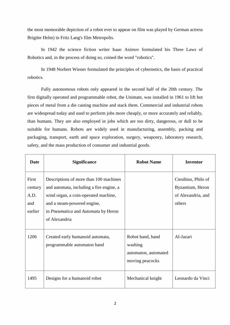
Date Significance Robot Name Inventor

First

century

A.D.

and

earlier

Descriptions of more than 100 machines

and automata, including a fire engine, a

wind organ, a coin-operated machine,

and a steam-powered engine,

in Pneumatica and Automata by Heron

of Alexandria

Ctesibius, Philo of

Byzantium, Heron

of Alexandria, and

others

1206 Created early humanoid automata,

programmable automaton band

Robot band, hand

washing

automaton, automated

moving peacocks

Al-Jazari

1495 Designs for a humanoid robot Mechanical knight Leonardo da Vinci

http://en.wikipedia.org/wiki/Hero_of_Alexandria

http://en.wikipedia.org/wiki/Hero_of_Alexandria

http://en.wikipedia.org/wiki/Ctesibius

http://en.wikipedia.org/wiki/Philo_of_Byzantium

http://en.wikipedia.org/wiki/Philo_of_Byzantium

http://en.wikipedia.org/wiki/Al-Jazari

http://en.wikipedia.org/wiki/Leonardo_da_Vinci

3

1738 Mechanical duck that was able to eat,

flap its wings, and excrete

Digesting Duck Jacques de

Vaucanson

1898 Nikola Tesla demonstrates first radio-

controlled vessel.

Teleautomaton Nikola Tesla

1921 First fictional automatons called "robots"

appear in the play R.U.R.

Rossum's Universal

Robots

Karel Čapek

1930s Humanoid robot exhibited at the 1939

and 1940 World's Fairs

Elektro Westinghouse

Electric Corporation

1948 Simple robots exhibiting biological

behaviors

Elsie and Elmer William Grey

Walter

1956 First commercial robot,from the

Unimation company founded by George

Devol and Joseph Engelberger, based on

Devol's patents

Unimate George Devol

1961 First installed industrial robot. Unimate George Devol

1963 First palletizing robot Palletizer Fuji Yusoki Kogyo

1973 First industrial robot with six

electromechanically driven axes

Famulus KUKA Robot

Group

1975 Programmable universal manipulation

arm, a Unimation product

PUMA Victor Scheinman

http://en.wikipedia.org/wiki/Digesting_Duck

http://en.wikipedia.org/wiki/Jacques_de_Vaucanson

http://en.wikipedia.org/wiki/Jacques_de_Vaucanson

http://en.wikipedia.org/wiki/Nikola_Tesla

http://en.wikipedia.org/wiki/Rossum%27s_Universal_Robots

http://en.wikipedia.org/wiki/Rossum%27s_Universal_Robots

http://en.wikipedia.org/wiki/Karel_%C4%8Capek

http://en.wikipedia.org/wiki/Expo_(exhibition)

http://en.wikipedia.org/wiki/Elektro

http://en.wikipedia.org/wiki/Westinghouse_Electric_(1886)

http://en.wikipedia.org/wiki/Westinghouse_Electric_(1886)

http://en.wikipedia.org/wiki/William_Grey_Walter

http://en.wikipedia.org/wiki/William_Grey_Walter

http://en.wikipedia.org/wiki/George_Devol


http://en.wikipedia.org/wiki/Joseph_Engelberger

http://en.wikipedia.org/wiki/Unimate


http://en.wikipedia.org/wiki/Unimate


http://en.wikipedia.org/wiki/Palletizer

http://en.wikipedia.org/w/index.php?title=Fuji_Yusoki_Kogyo&action=edit&redlink=1

http://en.wikipedia.org/wiki/Industrial_robot

http://en.wikipedia.org/wiki/KUKA

http://en.wikipedia.org/wiki/KUKA

http://en.wikipedia.org/wiki/Programmable_Universal_Machine_for_Assembly

http://en.wikipedia.org/wiki/Victor_Scheinman

4

2009 Largest and strongest industrial

robot with six axes

M-2000iA FANUC Robotics

America

Table 1 : History of robot inventions

1.2. Types and classification of robots

It is classified into six categories:

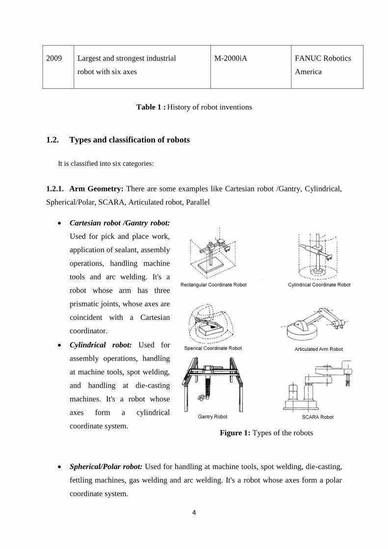
1.2.1. Arm Geometry: There are some examples like Cartesian robot /Gantry, Cylindrical,

Spherical/Polar, SCARA, Articulated robot, Parallel

Cartesian robot /Gantry robot:

Used for pick and place work,

application of sealant, assembly

operations, handling machine

tools and arc welding. It's a

robot whose arm has three

prismatic joints, whose axes are

coincident with a Cartesian

coordinator.

Cylindrical robot: Used for

assembly operations, handling

at machine tools, spot welding,

and handling at die-casting

machines. It's a robot whose

axes form a cylindrical

coordinate system.

Spherical/Polar robot: Used for handling at machine tools, spot welding, die-casting,

fettling machines, gas welding and arc welding. It's a robot whose axes form a polar

coordinate system.

Figure 1: Types of the robots



http://en.wikipedia.org/wiki/FANUC_Robotics_America_Corporation

http://en.wikipedia.org/wiki/FANUC_Robotics_America_Corporation

5

SCARA robot: Used for pick and place work, application of sealant, assembly

operations and handling machine tools. It's a robot which has two parallel rotary joints

to provide compliance in a plane.

Articulated robot: Used for assembly operations, die-casting, fettling machines, gas

welding, arc welding and spray painting. It's a robot whose arm has at least three

rotary joints.

Parallel robot: One use is a mobile platform handling cockpit flight simulators. It's a

robot whose arms have concurrent prismatic or rotary joints.

1.2.2. Degrees of freedom: It can be classified as Robot Arm, Robot Wrist.

1.2.3. Power sources: Electrical, Pneumatic; Hydraulic, Any Combination can be used as a

power source in robotic.

1.2.4. Type of motion: Slew Motion, Joint-Interpolation, Straight-Line Interpolation,

Circular Interpolation are the main motion types in current robotic area.

1.2.5. Path control: Limited sequence, point-to-point, continuous path, controlled path are

the most important and common ways in today‟s robotic world.

1.2.6. Intellligence level: Low-technology (nonservo), high-technology (servo) can be

classified as the level of intelligence of the robots.

6

2. AL5A robot arm

2.1. Features of the AL5A robot arm

Fast repeatable movements can be created by the AL5A robotic arm. The robot

features consist of base rotation, single plane shoulder, elbow, wrist motion, a functional

gripper, and optional wrist rotate. The AL5A robotic arm is an affordable system with a time

tested rock solid design that will last and last. Everything needed to assemble and operate the

robot is included in the kit, with several different software control options.

2.1.1. The Mechanics of the robot

Servo erector set components make the aluminum robotic arm ultimate in flexibility

and expandability. The kit consists of custom injection molded components, aluminum tubing

and hubs, black anodized aluminum brackets , and precision laser-cut Lexan components. The

arm uses 1 x HS-422 in the base, 1 x HS-755HB in the shoulder, 1 x HS-645MG in the elbow,

1 x HS-422 in the wrist, and 1 x HS-422 in the gripper.

2.1.2. The Electrical system of the robot

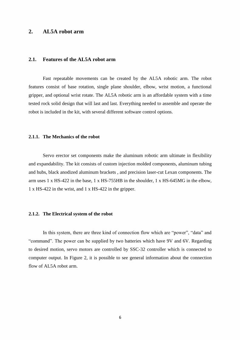
In this system, there are three kind of connection flow which are “power”, “data” and

“command”. The power can be supplied by two batteries which have 9V and 6V. Regarding

to desired motion, servo motors are controlled by SSC-32 controller which is connected to

computer output. In Figure 2, it is possible to see general information about the connection

flow of AL5A robot arm.

7

Figure 2 : The overview of the robot electrical system

2.1.3. Arm control options

There are three arm control options. Each of them have their own unique operating

feature sets. They all incorporate advanced Inverse Kinematics to easily and accurately

position the end effector in 3D space.

The first option is The Dual Lynx Arm Controller program which can be downloaded

freely. It allows AL5A arm to be controlled from a single SSC-32 servo controller. It allows

the creation and full editing of sequences of motion and steps. It uses a teach pendant style

control panel to emulate an industrial arm control system. It is also included the FlowStone

source code so the functionality to suit each purpose can be modified and customized.

The second option is to control with FlowArm program. It currently supports a single

AL5A arm with an SSC-32. It stores sequences of motion and allows full editing of sequence

steps. It uses a cool 2D, side view and top view graphical representation of the arm that is a

click or click-and-drag positioning system. FlowStone source code is available when

purchasing any version of FlowStone.

http://www.lynxmotion.com/p-822-free-download-lynx-arm-calibration-control.aspx

http://www.lynxmotion.com/p-821-free-download-flowarm-software.aspx

8

The third and most common option is RIOS which is operating system of robot with

also export and import options.. With RIOS, your robot can be taught sequences of motion via

the mouse or joystick. The inverse kinematics engine makes positioning the arm effortless.

This program uses external digital and analog inputs to affect the robot's motion for closed

loop projects. If-then, for-next, and do-while, are supported for the inputs. External outputs

can also be controlled. If stand alone operation is desired, RIOS/SSC-32 can actually create

the BASIC code to control the arm from our Bot Board and Basic Atom or Basic Stamp 2.

To have an alternative, the servo motors can also be controlled directly from a

microcontroller.

http://www.lynxmotion.com/p-419-rios-ssc-32-arm-control-software.aspx

9

2.2. Assembly of the AL5A robot arm

2.2.1. Assembly of the base:

Step-1 : As initial step of the assembly, base bearings are created as in Figure 3.

Figure 3 : Base bearings attachments

Step-2 : It should be installed the bearings into the base in the following Figure 4.

They will fit snugly. It is noted the notch in the bottom edge of the base indicates the back.

Figure 4 : Base

Step 3 : It is important lay a piece of 400 grit sandpaper on a flat surface and move the

base (upside down) in small circles on it. This will remove any imperfections on the bearings.

Figure 5 : Base mounting

10

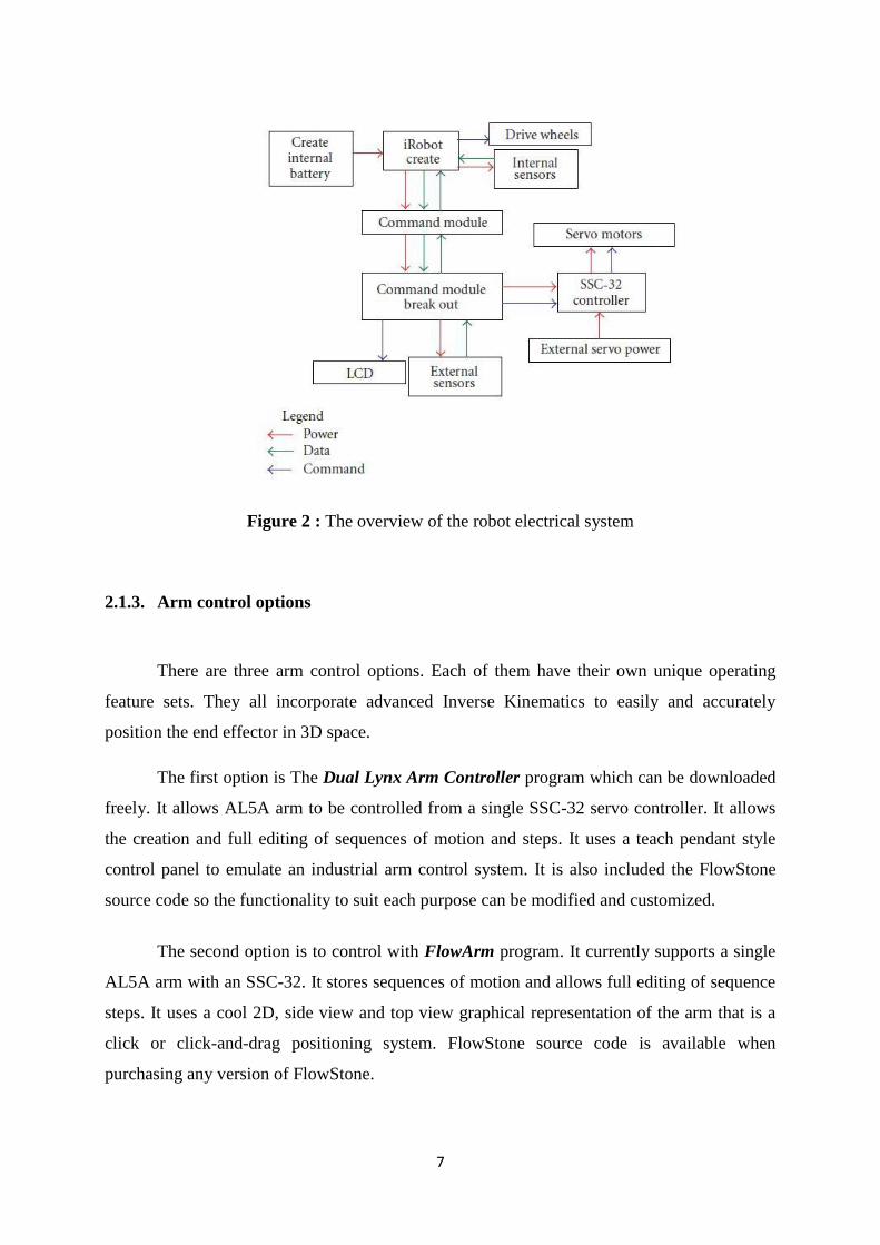
Step 4 : Figure 6 shows the circle pattern on the sandpaper and the inset shows the :

bearings after any imperfections have been removed.

Figure 6 : Base bearings

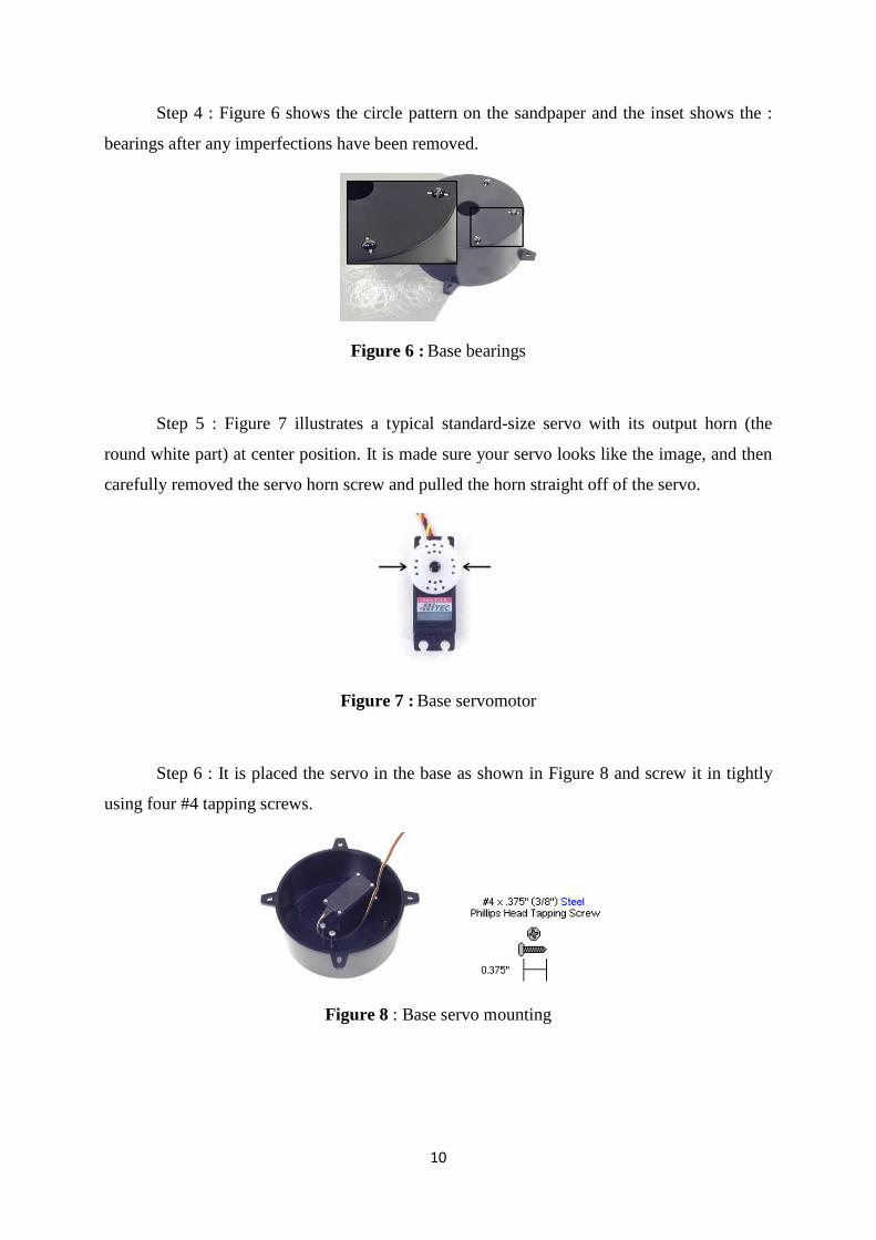
Step 5 : Figure 7 illustrates a typical standard-size servo with its output horn (the

round white part) at center position. It is made sure your servo looks like the image, and then

carefully removed the servo horn screw and pulled the horn straight off of the servo.

Figure 7 : Base servomotor

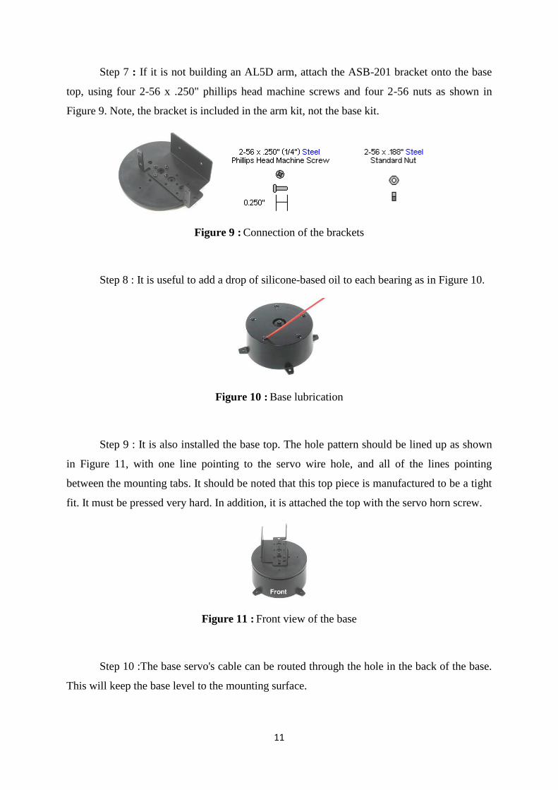
Step 6 : It is placed the servo in the base as shown in Figure 8 and screw it in tightly

using four #4 tapping screws.

Figure 8 : Base servo mounting

11

Step 7 : If it is not building an AL5D arm, attach the ASB-201 bracket onto the base

top, using four 2-56 x .250" phillips head machine screws and four 2-56 nuts as shown in

Figure 9. Note, the bracket is included in the arm kit, not the base kit.

Figure 9 : Connection of the brackets

Step 8 : It is useful to add a drop of silicone-based oil to each bearing as in Figure 10.

Figure 10 : Base lubrication

Step 9 : It is also installed the base top. The hole pattern should be lined up as shown

in Figure 11, with one line pointing to the servo wire hole, and all of the lines pointing

between the mounting tabs. It should be noted that this top piece is manufactured to be a tight

fit. It must be pressed very hard. In addition, it is attached the top with the servo horn screw.

Figure 11 : Front view of the base

Step 10 :The base servo's cable can be routed through the hole in the back of the base.

This will keep the base level to the mounting surface.

12

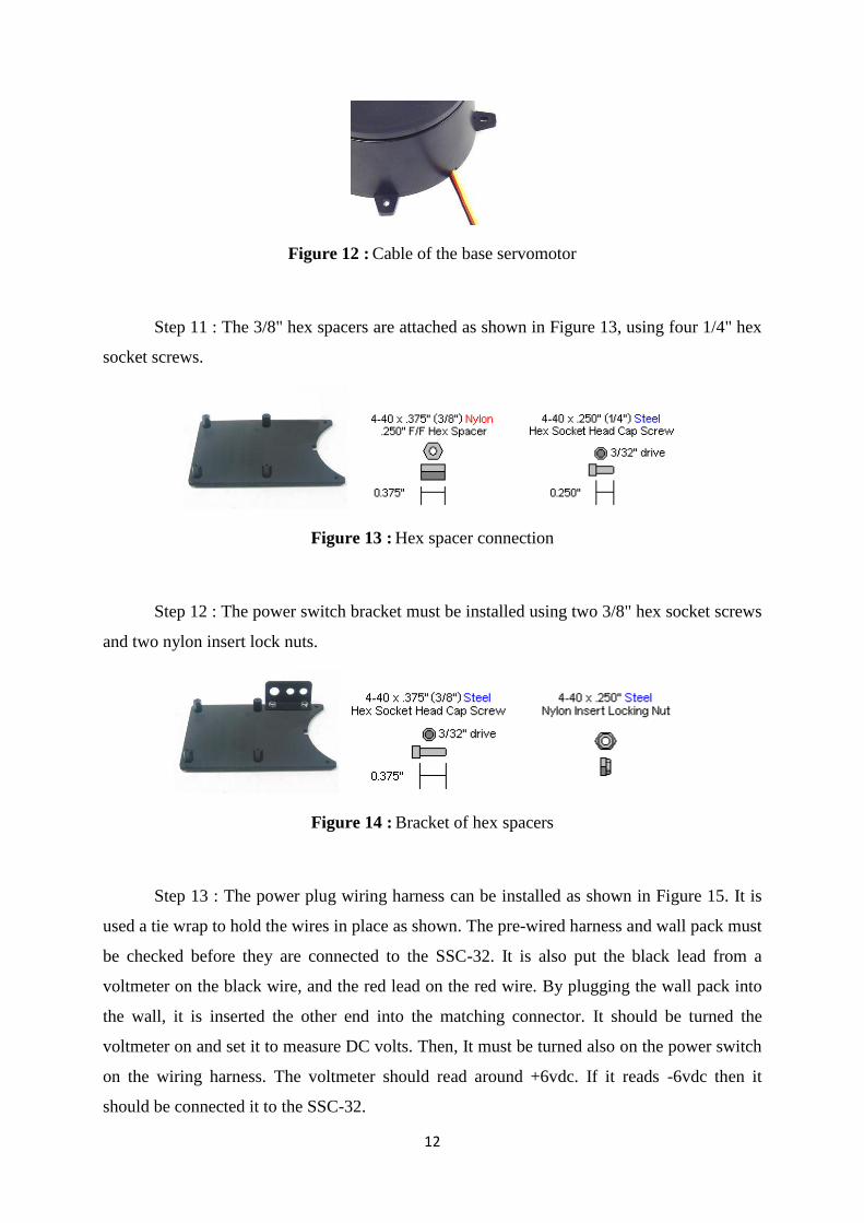
Figure 12 : Cable of the base servomotor

Step 11 : The 3/8" hex spacers are attached as shown in Figure 13, using four 1/4" hex

socket screws.

Figure 13 : Hex spacer connection

Step 12 : The power switch bracket must be installed using two 3/8" hex socket screws

and two nylon insert lock nuts.

Figure 14 : Bracket of hex spacers

Step 13 : The power plug wiring harness can be installed as shown in Figure 15. It is

used a tie wrap to hold the wires in place as shown. The pre-wired harness and wall pack must

be checked before they are connected to the SSC-32. It is also put the black lead from a

voltmeter on the black wire, and the red lead on the red wire. By plugging the wall pack into

the wall, it is inserted the other end into the matching connector. It should be turned the

voltmeter on and set it to measure DC volts. Then, It must be turned also on the power switch

on the wiring harness. The voltmeter should read around +6vdc. If it reads -6vdc then it

should be connected it to the SSC-32.

13

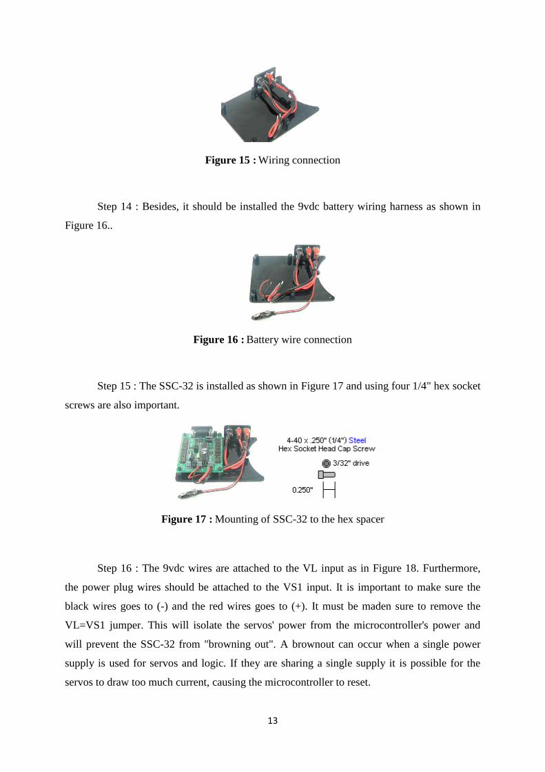
Figure 15 : Wiring connection

Step 14 : Besides, it should be installed the 9vdc battery wiring harness as shown in

Figure 16..

Figure 16 : Battery wire connection

Step 15 : The SSC-32 is installed as shown in Figure 17 and using four 1/4" hex socket

screws are also important.

Figure 17 : Mounting of SSC-32 to the hex spacer

Step 16 : The 9vdc wires are attached to the VL input as in Figure 18. Furthermore,

the power plug wires should be attached to the VS1 input. It is important to make sure the

black wires goes to (-) and the red wires goes to (+). It must be maden sure to remove the

VL=VS1 jumper. This will isolate the servos' power from the microcontroller's power and

will prevent the SSC-32 from "browning out". A brownout can occur when a single power

supply is used for servos and logic. If they are sharing a single supply it is possible for the

servos to draw too much current, causing the microcontroller to reset.

14

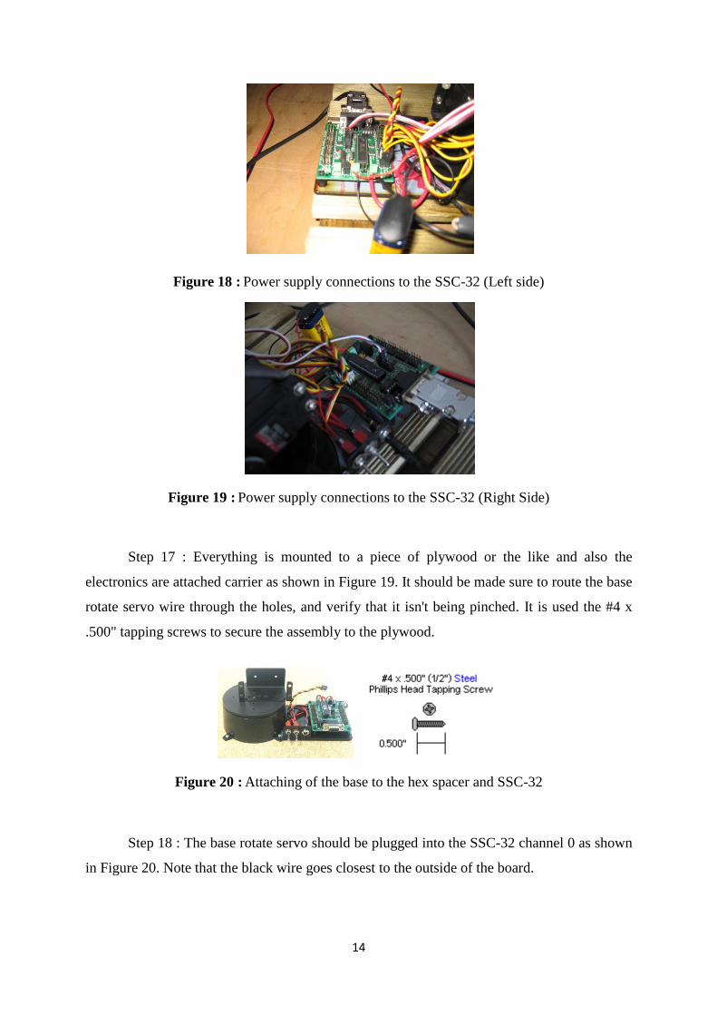
Figure 18 : Power supply connections to the SSC-32 (Left side)

Figure 19 : Power supply connections to the SSC-32 (Right Side)

Step 17 : Everything is mounted to a piece of plywood or the like and also the

electronics are attached carrier as shown in Figure 19. It should be made sure to route the base

rotate servo wire through the holes, and verify that it isn't being pinched. It is used the #4 x

.500" tapping screws to secure the assembly to the plywood.

Figure 20 : Attaching of the base to the hex spacer and SSC-32

Step 18 : The base rotate servo should be plugged into the SSC-32 channel 0 as shown

in Figure 20. Note that the black wire goes closest to the outside of the board.

15

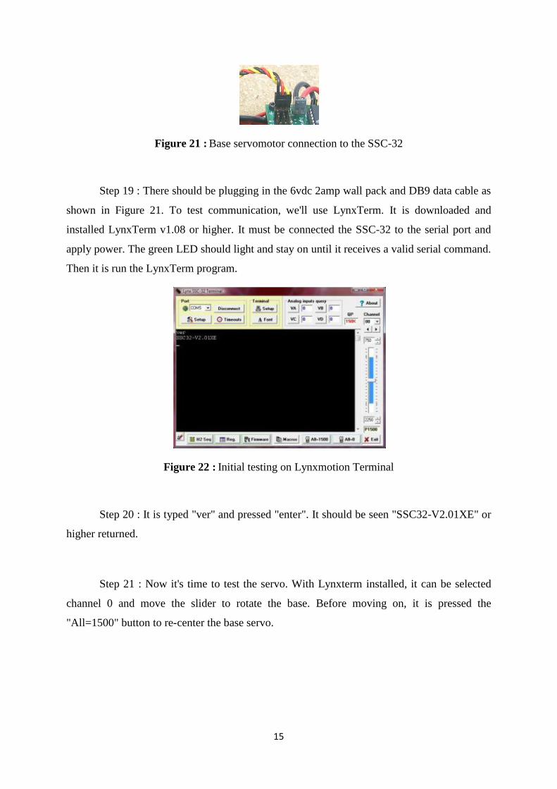
Figure 21 : Base servomotor connection to the SSC-32

Step 19 : There should be plugging in the 6vdc 2amp wall pack and DB9 data cable as

shown in Figure 21. To test communication, we'll use LynxTerm. It is downloaded and

installed LynxTerm v1.08 or higher. It must be connected the SSC-32 to the serial port and

apply power. The green LED should light and stay on until it receives a valid serial command.

Then it is run the LynxTerm program.

Figure 22 : Initial testing on Lynxmotion Terminal

Step 20 : It is typed "ver" and pressed "enter". It should be seen "SSC32-V2.01XE" or

higher returned.

Step 21 : Now it's time to test the servo. With Lynxterm installed, it can be selected

channel 0 and move the slider to rotate the base. Before moving on, it is pressed the

"All=1500" button to re-center the base servo.

16

Figure 23 : Completed mounting of base, hex spacer and SSC-32

2.2.2. Assembly of the arm :

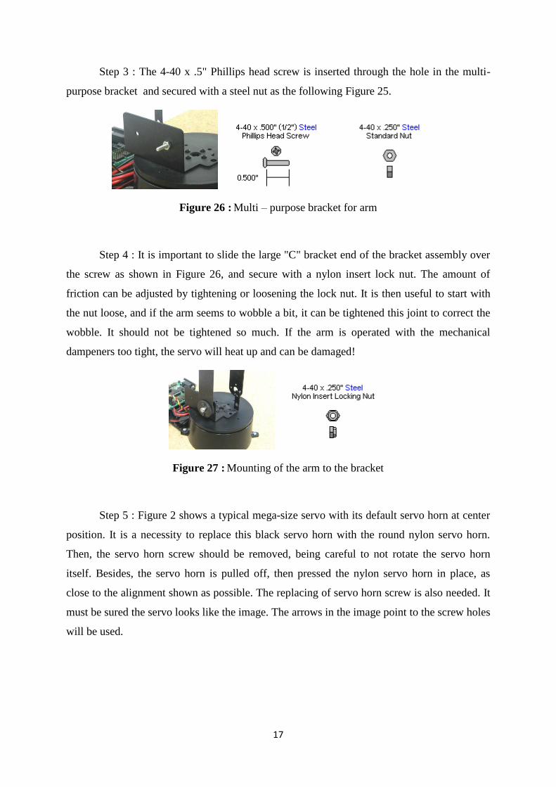
Step 1 : The "C" bracket is connected to the large "C" bracket as shown in Figure 23

by using two 2-56 x 1/4" screws and 2-56 nuts.

Figure 24 : C bracket screws and nuts

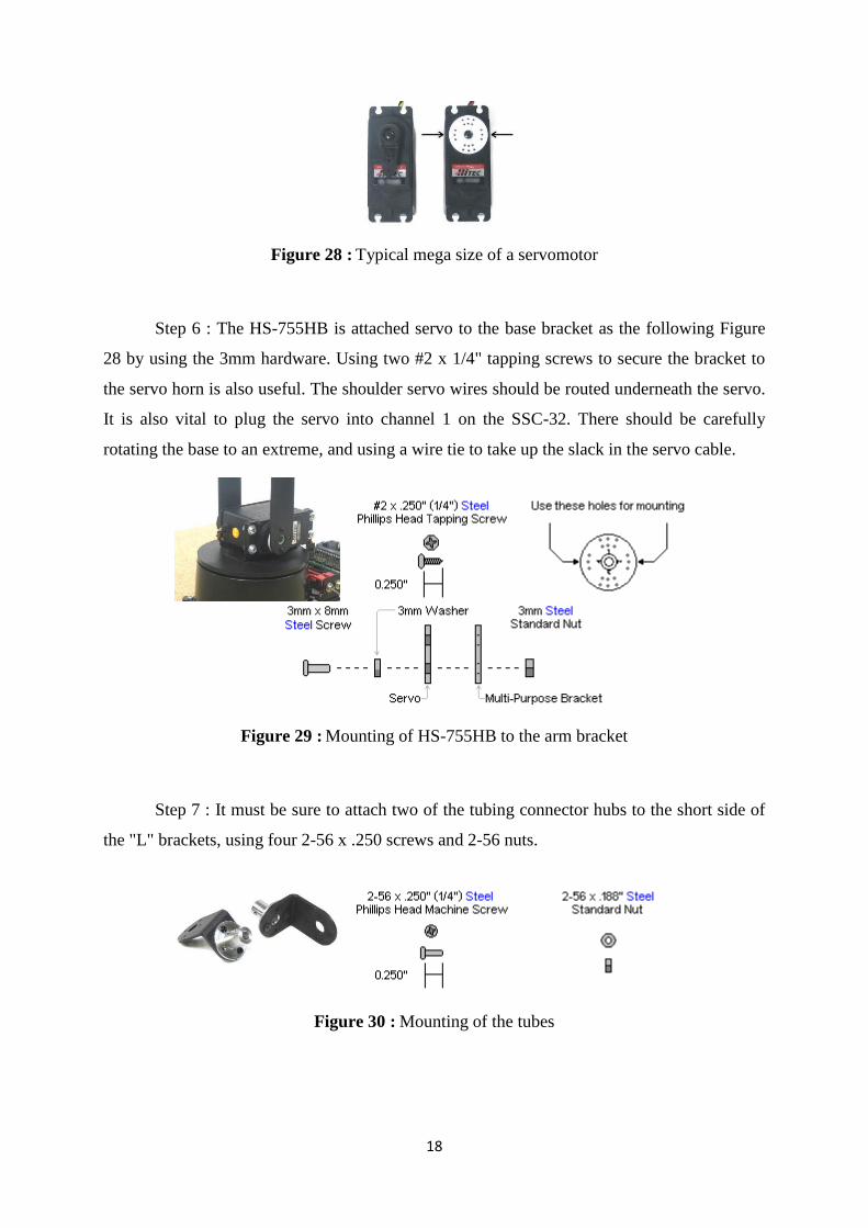
Step 2 : The mechanical dampening panels are installed as follows in Figure 24 by

using four tapping screws.

Figure 25 : Dampening panels

17

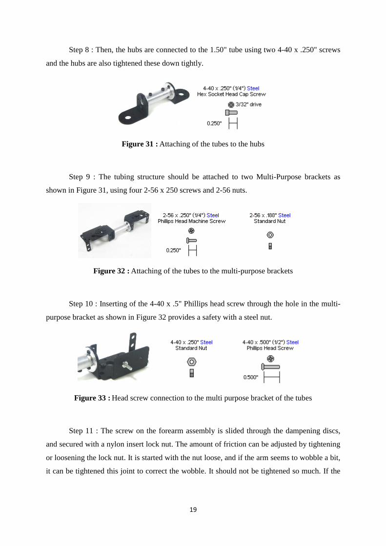
Step 3 : The 4-40 x .5" Phillips head screw is inserted through the hole in the multi-

purpose bracket and secured with a steel nut as the following Figure 25.

Figure 26 : Multi – purpose bracket for arm

Step 4 : It is important to slide the large "C" bracket end of the bracket assembly over

the screw as shown in Figure 26, and secure with a nylon insert lock nut. The amount of

friction can be adjusted by tightening or loosening the lock nut. It is then useful to start with

the nut loose, and if the arm seems to wobble a bit, it can be tightened this joint to correct the

wobble. It should not be tightened so much. If the arm is operated with the mechanical

dampeners too tight, the servo will heat up and can be damaged!

Figure 27 : Mounting of the arm to the bracket

Step 5 : Figure 2 shows a typical mega-size servo with its default servo horn at center

position. It is a necessity to replace this black servo horn with the round nylon servo horn.

Then, the servo horn screw should be removed, being careful to not rotate the servo horn

itself. Besides, the servo horn is pulled off, then pressed the nylon servo horn in place, as

close to the alignment shown as possible. The replacing of servo horn screw is also needed. It

must be sured the servo looks like the image. The arrows in the image point to the screw holes

will be used.

18

Figure 28 : Typical mega size of a servomotor

Step 6 : The HS-755HB is attached servo to the base bracket as the following Figure

28 by using the 3mm hardware. Using two #2 x 1/4" tapping screws to secure the bracket to

the servo horn is also useful. The shoulder servo wires should be routed underneath the servo.

It is also vital to plug the servo into channel 1 on the SSC-32. There should be carefully

rotating the base to an extreme, and using a wire tie to take up the slack in the servo cable.

Figure 29 : Mounting of HS-755HB to the arm bracket

Step 7 : It must be sure to attach two of the tubing connector hubs to the short side of

the "L" brackets, using four 2-56 x .250 screws and 2-56 nuts.

Figure 30 : Mounting of the tubes

19

Step 8 : Then, the hubs are connected to the 1.50" tube using two 4-40 x .250" screws

and the hubs are also tightened these down tightly.

Figure 31 : Attaching of the tubes to the hubs

Step 9 : The tubing structure should be attached to two Multi-Purpose brackets as

shown in Figure 31, using four 2-56 x 250 screws and 2-56 nuts.

Figure 32 : Attaching of the tubes to the multi-purpose brackets

Step 10 : Inserting of the 4-40 x .5" Phillips head screw through the hole in the multi-

purpose bracket as shown in Figure 32 provides a safety with a steel nut.

Figure 33 : Head screw connection to the multi purpose bracket of the tubes

Step 11 : The screw on the forearm assembly is slided through the dampening discs,

and secured with a nylon insert lock nut. The amount of friction can be adjusted by tightening

or loosening the lock nut. It is started with the nut loose, and if the arm seems to wobble a bit,

it can be tightened this joint to correct the wobble. It should not be tightened so much. If the

20

arm is operated with the mechanical dampeners too tight, the servo will heat up and can be

damaged.

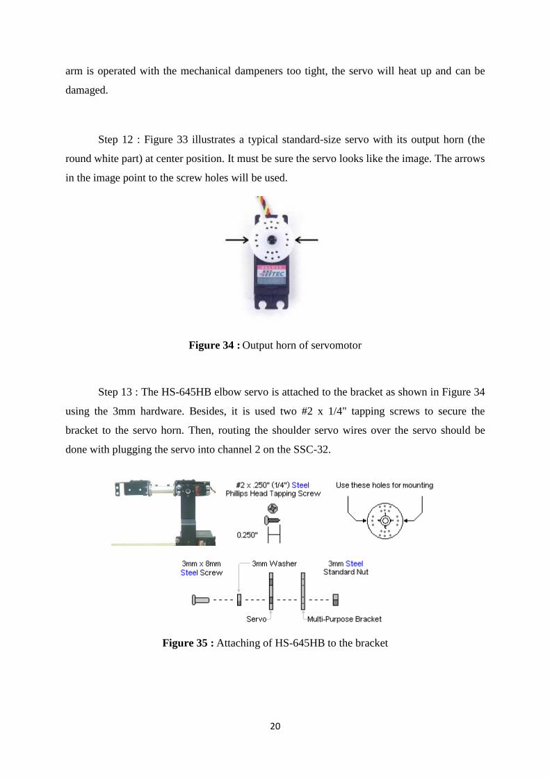
Step 12 : Figure 33 illustrates a typical standard-size servo with its output horn (the

round white part) at center position. It must be sure the servo looks like the image. The arrows

in the image point to the screw holes will be used.

Figure 34 : Output horn of servomotor

Step 13 : The HS-645HB elbow servo is attached to the bracket as shown in Figure 34

using the 3mm hardware. Besides, it is used two #2 x 1/4" tapping screws to secure the

bracket to the servo horn. Then, routing the shoulder servo wires over the servo should be

done with plugging the servo into channel 2 on the SSC-32.

Figure 35 : Attaching of HS-645HB to the bracket

21

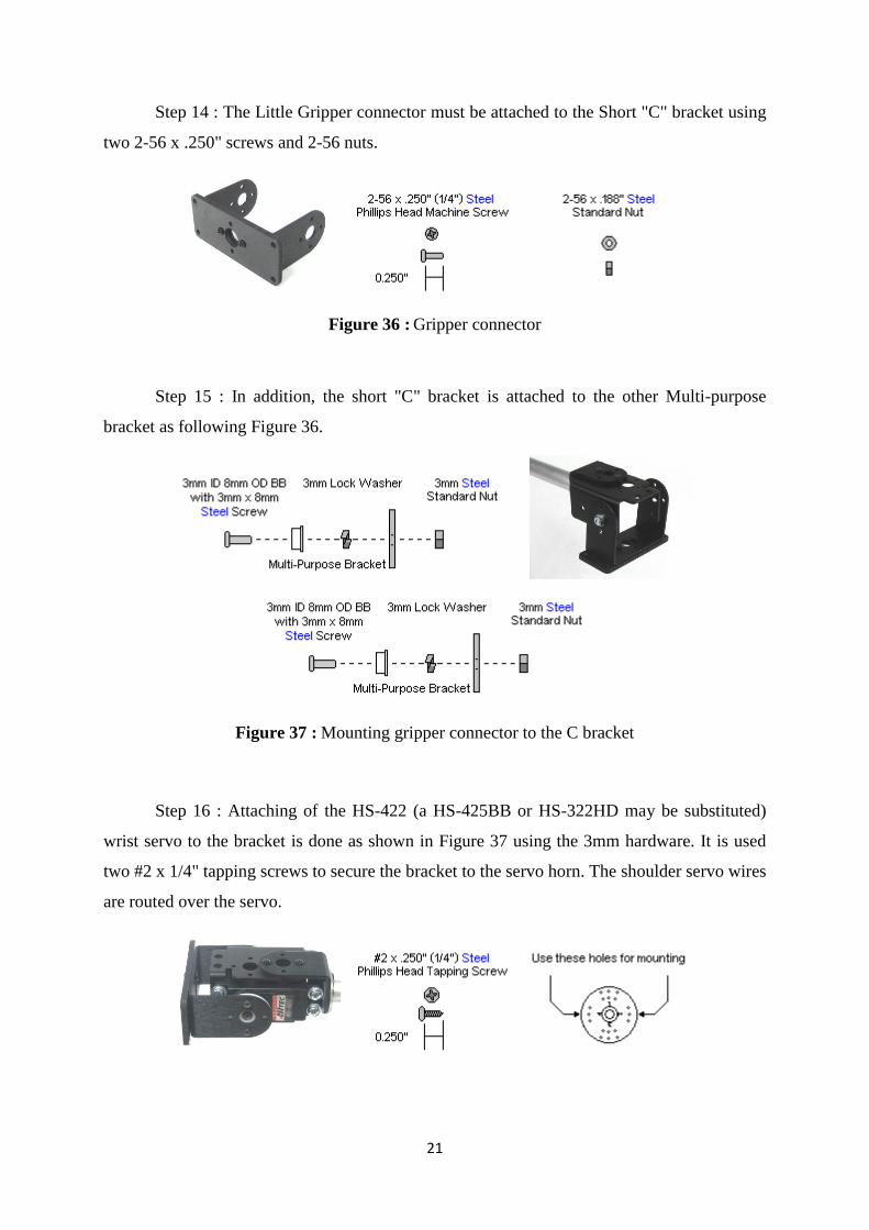
Step 14 : The Little Gripper connector must be attached to the Short "C" bracket using

two 2-56 x .250" screws and 2-56 nuts.

Figure 36 : Gripper connector

Step 15 : In addition, the short "C" bracket is attached to the other Multi-purpose

bracket as following Figure 36.

Figure 37 : Mounting gripper connector to the C bracket

Step 16 : Attaching of the HS-422 (a HS-425BB or HS-322HD may be substituted)

wrist servo to the bracket is done as shown in Figure 37 using the 3mm hardware. It is used

two #2 x 1/4" tapping screws to secure the bracket to the servo horn. The shoulder servo wires

are routed over the servo.

22

Figure 38 : Attaching of HS-422 to the C bracket

Step 17 : The Little Grip must be attached to the lexan as shown in Figure 38, using

three 4-40 x .375" button head screws and acorn locking nuts. Only three screws are used

(shown in the image) as the body of the gripper servo is in the way for the fourth.

Figure 39 : Little grip

It must be secured that the HS-422 (a HS-322HD may be substituted) servo is aligned

to mid-position, and the gripper is halfway open. Now the servo and gripper will be aligned

correctly. The servo screw and horn should be removed and the servo must be slided into the

gripper from the bottom. It is also necessity to wiggle it a bit to get it seated properly. By

using the servo screw to attach the servo, it is tightened this down, but then unscrew it half a

turn. Too much friction can bind the servo.

Step 18 : 6th servo extender cables are added to the wrist and gripper servos.

Figure 40 : Extender cables for 6th servo

23

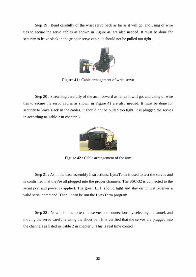
Step 19 : Bend carefully of the wrist servo back as far as it will go, and using of wire

ties to secure the servo cables as shown in Figure 40 are also needed. It must be done for

security to leave slack in the gripper servo cable, it should not be pulled too tight.

Figure 41 : Cable arrangement of wrist servo

Step 20 : Stretching carefully of the arm forward as far as it will go, and using of wire

ties to secure the servo cables as shown in Figure 41 are also needed. It must be done for

security to leave slack in the cables, it should not be pulled too tight. It is plugged the servos

in according to Table 2 in chapter 3.

Figure 42 : Cable arrangement of the arm

Step 21 : As in the base assembly Instructions, LynxTerm is used to test the servos and

is confirmed that they're all plugged into the proper channels. The SSC-32 is connected to the

serial port and power is applied. The green LED should light and stay on until it receives a

valid serial command. Then, it can be run the LynxTerm program.

Step 22 : Now it is time to test the servos and connections by selecting a channel, and

moving the servo carefully using the slider bar. It is verified that the servos are plugged into

the channels as listed in Table 2 in chapter 3. This is real time control.

24

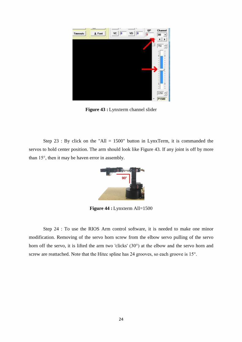
Figure 43 : Lynxterm channel slider

Step 23 : By click on the "All = 1500" button in LynxTerm, it is commanded the

servos to hold center position. The arm should look like Figure 43. If any joint is off by more

than 15°, then it may be haven error in assembly.

Figure 44 : Lynxterm All=1500

Step 24 : To use the RIOS Arm control software, it is needed to make one minor

modification. Removing of the servo horn screw from the elbow servo pulling of the servo

horn off the servo, it is lifted the arm two 'clicks' (30°) at the elbow and the servo horn and

screw are reattached. Note that the Hitec spline has 24 grooves, so each groove is 15°.

25

Figure 45 : Arrangement of the arm for RIOS

Step 25 : At this point the arms is assembled and tested using LynxTerm. Now it is

needed to install the RIOS and calibrate the arm to the software. It is important to do an

accurate calibration. The performance of the arm will only be as good as the calibration. If the

on screen virtual arm does not match the real arm this is a sign of an inaccurate calibration.

After calibration studying of the RIOS manual carefully is beneficial to learn how to store and

playback sequences for the arm.

Figure 46 : RIOS interface

Step 26 : To calibrate the arm's Shoulder servo, it is clicked the "SSC-32" button.

Step 27 : It is selected the Shoulder, servo #2 and is moved the shoulder slider up to

move the shoulder forward so that it looks like Figure 44. After setting the Min Deg angle -

90°, by right click on the slider to set this as the Min Position, the servo will not go past this

value, and the program now knows this value is exactly 90° from centered.

26

Figure 47 : SSC-32 link on RIOS

Figure 48 : Initial arm calibration

It is time to move the slider down to move the shoulder backward so that it looks like

Figure 47. After setting again the Max Deg angle to 45°, by right click on the slider to set this

as the Max Position, the servo will not go past this value, and the program now knows this

value is exactly 45° from centered.

Step 28 : To connect springs for load-balancing, it is replaced the servo attachment

hardware in the locations shown, following the Figure 48 below. The springs should be

hooked together after they're secured.

27

Figure 49 : Spring connection of the arm

Step 29 : The arm assembly is complete. It is accessible by clicking on the help icon

on the main screen or by navigating to the install directory (c:\Program Files\RIOS_SSC-32\)

and opening the Help.pdf file. This manual explains in great detail how to use the arm. The

arm is robust mechanically, but the servos can be damaged by improper use. An example

would be if the arm was told to move to an unobtainable position, like the surface the arm is

mounted to, or by crashing the arm into itself, or other objects. The elbow servo is the most

vulnerable because it holds the entire weight of the forearm. Load balancing springs should be

added to reduce some of this load. It should also be remembered, the most important rule for

servo based robot arm are parking the arm when not in motion. When it's moving or at rest it's

usually ok. When it's holding an object it should do so for the minimum amount of time

required to do the job. It can always touched the servo case to see if it's getting hot.

2.2.3. Assembly for heavy-duty motion :

Step 1 : The gripper assembly is removed from the "C" bracket to the little grip. Also

the little grip is removed from the little grip adapter, and the little grip adapter is finally

removed from the "C" bracket.

28

Step 2 : It is referred to the ball bearing hub and low profile axis assembly guide to

build the assembly. It must be used the "C" bracket you just removed from the arm and the

HS-475 or HS-485 servo included. In order to install the gripper, the full gear must also be

removed.

Figure 50 : Ball bearing hub

Step 3 : To space the gripper away from the gears, it is important to use the four

washers, two stacked on each side of the final gear. Aligning the bearing, gear, and washers as

shown in Figure 50 to prepare to install the little grip attachment plate is done.

Figure 51 : Gears of the wrist rotation

Step 4 : Installing of the little grip attachment plate as shown in Figure 51 should be

done, using the 2-56 x .375" screws.

Figure 52 : Grip attachment plate to the gears

29

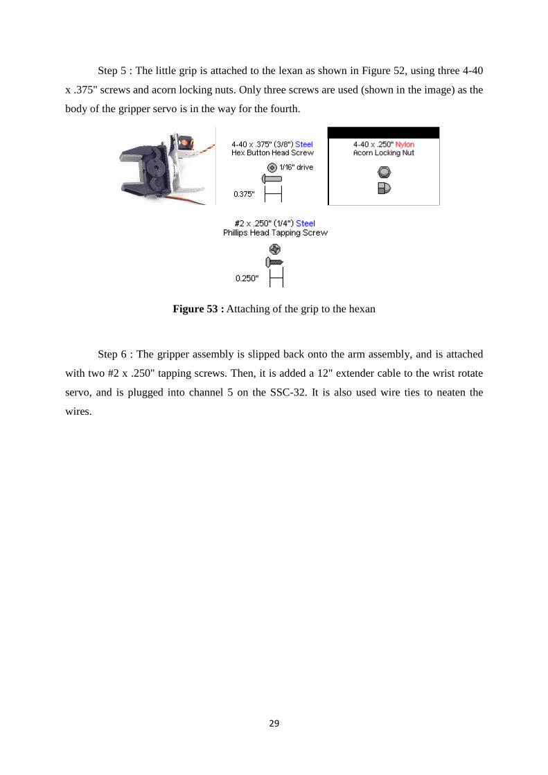
Step 5 : The little grip is attached to the lexan as shown in Figure 52, using three 4-40

x .375" screws and acorn locking nuts. Only three screws are used (shown in the image) as the

body of the gripper servo is in the way for the fourth.

Figure 53 : Attaching of the grip to the hexan

Step 6 : The gripper assembly is slipped back onto the arm assembly, and is attached

with two #2 x .250" tapping screws. Then, it is added a 12" extender cable to the wrist rotate

servo, and is plugged into channel 5 on the SSC-32. It is also used wire ties to neaten the

wires.

30

3. Controlling of AL5A with lynxmotion RIOS

Figure 54 : Panel of the program

3.1. Configuration of the SSC-32 card

Step 1. The RIOS program is installed. It is necessary to apply servo power to

complete the setup. Serial or serial to USB cable is connected, waited for the system to

recognize the card and the program is run. If the program was run before the system

recognized the card, the message box was seen "Can‟t find SSC card”. Then 'Yes' is clicked,

and the program will be enable the grayed buttons when the card is ready. If the card is not

detected, the right COM port number must be selected in the list box.

31

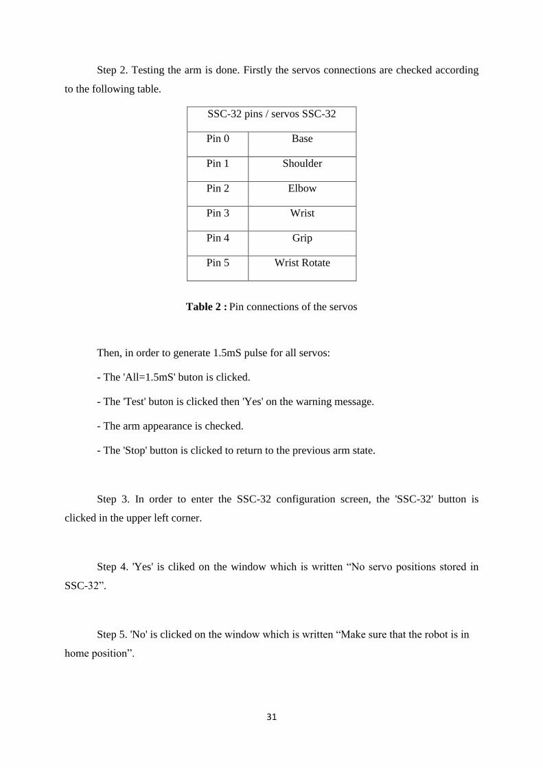
Step 2. Testing the arm is done. Firstly the servos connections are checked according

to the following table.

SSC-32 pins / servos SSC-32

Pin 0 Base

Pin 1 Shoulder

Pin 2 Elbow

Pin 3 Wrist

Pin 4 Grip

Pin 5 Wrist Rotate

Table 2 : Pin connections of the servos

Then, in order to generate 1.5mS pulse for all servos:

- The 'All=1.5mS' buton is clicked.

- The 'Test' buton is clicked then 'Yes' on the warning message.

- The arm appearance is checked.

- The 'Stop' button is clicked to return to the previous arm state.

Step 3. In order to enter the SSC-32 configuration screen, the 'SSC-32' button is

clicked in the upper left corner.

Step 4. 'Yes' is cliked on the window which is written “No servo positions stored in

SSC-32”.

Step 5. 'No' is clicked on the window which is written “Make sure that the robot is in

home position”.

32

Step 6. Adjusting the 'Min Pos' and the 'Max Pos' is done. The boxes in the top row

must be enable and also the robot power must be switched on.

Figure 55 : Adjusting Min and Max positions

Step 7. Configuration of the Base

Slider #1 is moved to the middle.

The robot base is manually moved to the middle.

The 'enable' checkbox #1 is checked, and the base moves a bit.

Slider #1 is slowly moved to the top and the base turns to the right. When the

slider is all the way at the top, the base must be at 90° to the right. If it is less than

this value, the 'Min Pos' box #1 is decreased. It allows to push the slider a bit more

to the top. If it is more, it is increased. It allows to push the slider down.

When it is finished, the same is done for the left. It must be full left (90°).

Finally the slider #1 must be at 0°.

33

Step 8. Configuration of the Shoulder


The robot shoulder is manually moved to the vertical position and it should be held

by hand for safe.

The 'enable' checkbox #2 is checked, and the shoulder moves a bit.

Slider #2 is slowly moved to the top and the arm must be at the front of the robot

and horizantal. The 'Min Pos' box #2 is adjusted if needed.

Slider #2 is slowly moved to the bottom and the arm must be at the rear of the

robot (45°). The 'Max Pos' box #2 is adjusted if needed.

Finally the slider #2 must be 0°.

Step 9. Configuration of the Elbow (forearm)


The robot forearm is manually moved to the horizontal position or vertical with

respect to shoulder. It should be held by hand for safe.

The 'enable' checkbox #3 is checked, and the elbow moves a bit.

Slider #3 is slowly moved to the top and the elbow must be slightly touching the

arm Hex Spacer. The 'Min Pos' box #3 is adjusted if needed.

Slider #3 is slowly moved to the bottom and the elbow must be at the rear of the

robot and horizontal. The 'Max Pos' box #3 is adjusted if needed.

Finally the slider #3 must be 0°.

Step 10. Configuration of the Wrist


The robot hand is manually moved to vertical with respect to shoulder. It should be

held by hand for safe.

The 'enable' checkbox #4 is checked, and the wrist moves a bit.

34

Slider #4 is slowly moved to the top and the hand must be at vertical with respect

to the forearm and below of it. The 'Min Pos' box #4 is adjusted if needed.

Slider #4 is slowly moved to the bottom and the hand must be at vertical with

respect to the forearm and above of it. The 'Max Pos' box #4 is adjusted if needed.

Finally the slider #4 must be -40° and the slider #3 must be changed as -65°.

Step 11. Configuration of the Gripper


The robot hand should not manually moved and it should be left how it is.

The 'enable' checkbox #5 is checked, and the gripper moves a bit.

Slider #5 is slowly moved to the top and the gripper must be fulley opened. The

'Min Pos' box #5 is adjusted if needed.

Slider #5 is slowly moved to the bottom and the gripper must be fulley closed. The

'Max Pos' box #5 is adjusted if needed.

Finally the slider #4 must be at 57° (the gripper should be half opened).

Step 12. Configuration of the Wrist Rotate


The robot wrist rotate should not manually moved and it should be left how it is.

The 'enable' checkbox #6 is checked, and the gripper moves a bit.

Slider #6 is slowly moved to the bottom and the gripper should be turned to left to

65°. The 'Max Pos' box #6 is adjusted if needed.

Slider #6 is slowly moved to the top and the gripper should be turned to right to

65°. The 'Max Pos' box #6 is adjusted if needed.

Finally the slider #6 must be at 0° (the gripper should be half opened).

Other values are entered for ‟'Min Deg' and 'Max Deg' and adjusted the Min Pos and

Max Pos to allow the robot to reach these values if wanted. However, it must be carefully to

not move the servos past its mechanical limits.

35

Step 13. In order to obtain default position, „Save‟ button must be clicked.

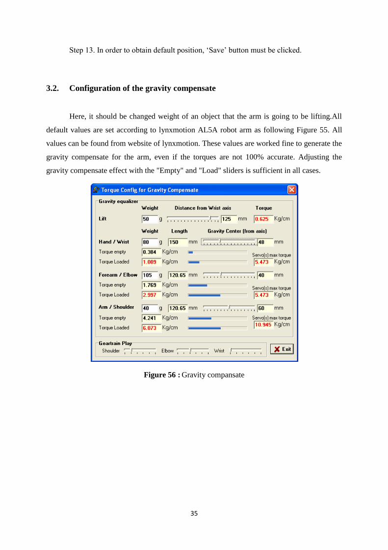
3.2. Configuration of the gravity compensate

Here, it should be changed weight of an object that the arm is going to be lifting.All

default values are set according to lynxmotion AL5A robot arm as following Figure 55. All

values can be found from website of lynxmotion. These values are worked fine to generate the

gravity compensate for the arm, even if the torques are not 100% accurate. Adjusting the

gravity compensate effect with the "Empty" and "Load" sliders is sufficient in all cases.

Figure 56 : Gravity compansate

36

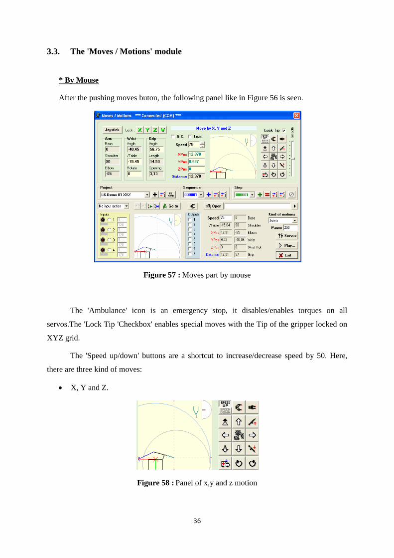
3.3. The 'Moves / Motions' module

* By Mouse

After the pushing moves buton, the following panel like in Figure 56 is seen.

Figure 57 : Moves part by mouse

The 'Ambulance' icon is an emergency stop, it disables/enables torques on all

servos.The 'Lock Tip 'Checkbox' enables special moves with the Tip of the gripper locked on

XYZ grid.

The 'Speed up/down' buttons are a shortcut to increase/decrease speed by 50. Here,

there are three kind of moves:

X, Y and Z.

Figure 58 : Panel of x,y and z motion

37

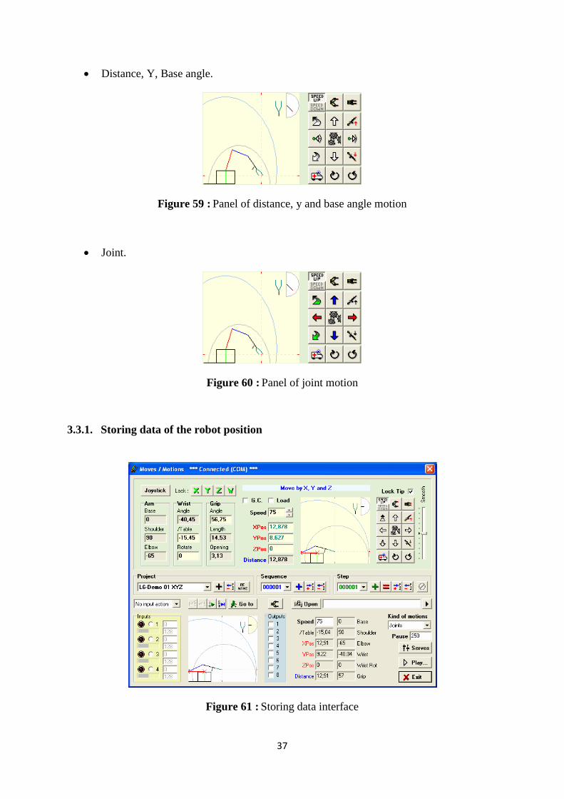
Distance, Y, Base angle.

Figure 59 : Panel of distance, y and base angle motion

Joint.

Figure 60 : Panel of joint motion

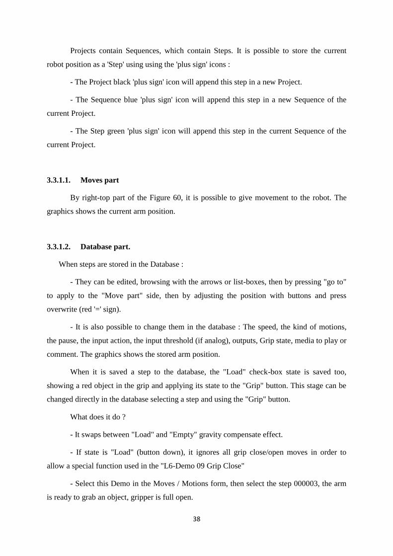
3.3.1. Storing data of the robot position

Figure 61 : Storing data interface

38

Projects contain Sequences, which contain Steps. It is possible to store the current

robot position as a 'Step' using using the 'plus sign' icons :

- The Project black 'plus sign' icon will append this step in a new Project.

- The Sequence blue 'plus sign' icon will append this step in a new Sequence of the

current Project.

- The Step green 'plus sign' icon will append this step in the current Sequence of the

current Project.

3.3.1.1. Moves part

By right-top part of the Figure 60, it is possible to give movement to the robot. The

graphics shows the current arm position.

3.3.1.2. Database part.

When steps are stored in the Database :

- They can be edited, browsing with the arrows or list-boxes, then by pressing "go to"

to apply to the "Move part" side, then by adjusting the position with buttons and press

overwrite (red '=' sign).

- It is also possible to change them in the database : The speed, the kind of motions,

the pause, the input action, the input threshold (if analog), outputs, Grip state, media to play or

comment. The graphics shows the stored arm position.

When it is saved a step to the database, the "Load" check-box state is saved too,

showing a red object in the grip and applying its state to the "Grip" button. This stage can be

changed directly in the database selecting a step and using the "Grip" button.

What does it do ?

- It swaps between "Load" and "Empty" gravity compensate effect.

- If state is "Load" (button down), it ignores all grip close/open moves in order to

allow a special function used in the "L6-Demo 09 Grip Close"

- Select this Demo in the Moves / Motions form, then select the step 000003, the arm

is ready to grab an object, gripper is full open.

39

- Now it is selected the step 000004, this move slowly and fully closes the gripper, an

input action is defined, expecting input #1 to occur to "stop this step".

- It is browsed now steps 000005 to 000007, these moves are carrying the object, the

"Grip" button is down so the Grip position stored in these 3 steps won't be used. These 3 steps

will be performed using the last grip position, that is the one stopped by the input #1 in the

step 000004. This feature allows to use a pressure sensor or a switch in the gripper to stop the

grip while closing, then carry the object discarding all further grip moves with the "Grip"

button pushed (useful when it is not known the object size).

- If it is seen now step 000008, this step fully opens the grip to drop the object, but

now the "Grip" button is release to allow this grip move. To try this feature, it is gone to the

"Play" form and is selected the "L6-Demo 09 Grip Close" project, by pressing the project's

Play button and waiting for the Step 000004 to start, it will say in the white status-bar:

"Waiting for input #1 to stop this move", press the input #1 button to simulate a

switch/pressure sensor and the grip close will stop.Then, depending on the moment you

pressed the button it will carry a larger or smaller object in the gripper.

3.3.2. Storing data of the features

It is used the combo-boxes to select a Project/Sequence/Step or use the four S-, I-, I+

and S+ icons to navigate through Sequences and Steps. 'Open' icon allows to add a media to

this Step, music or video, or it can be typed a little comment. It is test the media with the

black triangle icon. Speed is the one to reach this step. Pause (ms, 1000ms = 1 second) will be

performed at the end of Step, recommended value is 250 or more.

It is checked the Outputs check-boxes to set them On/Off (applied when starting the

Step). (Outputs 1 to 8 are Pin 8 to 15 on the SSC-32)

Kind of motion :

- "Joint" will perform curve trajectories and allows to move one joint only for

example. All "Home" positions should use "Joint" moves, it's the only one kind of motion

which won't hang in case of a joint is going to its limits during a travel and locks the move

(red cross on joint).

- "XYZ" will perform straight lines trajectories on the three axes.

40

- "Dist, Y, Base" will perform straight lines trajectories except the base rotation. Using

this kind of motion, the arm is carrying his "X axis" when the Base is moving, so the X axis is

renamed "Distance" (distance from base axis to gripper tip), then we are no more talking

about "Z" axis but a base rotation angle rather. To be short, it performs straight lines

trajectories in the vertical plan (Distance (from base axis) and Y (height)) and use a Base

angle to rotate this plan arround the vertical axis. The Moves panel will let you familiarize

with this three kind of moves (use the gears icon to swap kind of moves).

Figure 62 : Input preferences

It is selected an input action if needed.

- 'Wait for' means that robot will wait for an input to occur or a counter to reach a

value before starting the step.

- 'Pause/Play' means that robot will Swap between Pause and Play if an input occurs or

a counter reaches a value.

- 'Stop project' will stop the current Project if an input occurs or a counter reaches a

value.

- 'Stop this Step' will stop the current Step if an input occurs or a counter reaches a

value and go to the next Step.

It is selected an input to test and set a counter value.

- This version of RIOS allows only 'Relative' counter values and not 'Absolute'.

- So, if the counter value is set to '3', for example, the input selected must occur 3

times during the Step, no matter what the counter was at before the step.

41

3.4. The 'Play' module

3.4.1. Play features

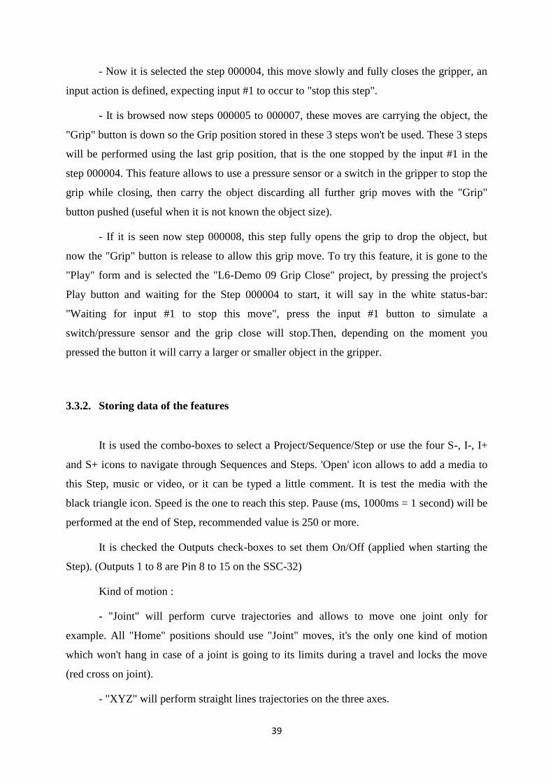
Figure 63 : Play module of RIOS

It is played a Project or a Sequence.Then, it is selected a position with the S-, I-, I+

and S+ icons.

'Go to' the position means the position that have been selected. It is selected 'inputs as

starter for sequence' and push the 'Scan' button, if a corresponding input occur, it will play the

Sequence selected (only if there's nothing already playing).

It can be built a Sequence list and can be played it. By options;

- Append If-Then-Else structure.

- Break a loop with If-Break instruction.

- Save a Sequence list by Project.

42

It can be clicked the robot picture to change the view. The robot picture shows the

current position and a ghost of the selected or next Step in Play mode. The Base, Shoulder,

Elbow and Wrist trajectories can be seen. Trigger inputs and watch outputs turn on and off. It

is possible to use 'Smooth' slider to eliminate shakes real time torques display. Outputs

configuration is with delays, durations and blink speed.

3.4.2. Output options

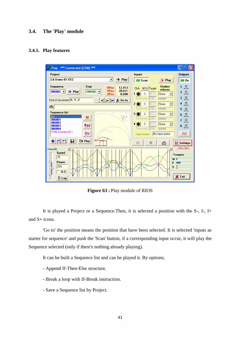
Figure 64 : Output options

Delay : When a Step sets an output on, this allows a delay before the output is

really set on.

Duration : When an output is really set on, it will auto set off after the Duration period

(if duration = 0 it will not auto set off).

Speed : If it is needed an output to blink, set a speed > 0. 1 is the slowest and 20 the

fastest, 0 is no blink. It is clicked on the test button to perform the Delay, then the blink/set

on, and after the duration, the auto set off

43

3.4.3. Sequence list

Figure 65 : Sequence interface

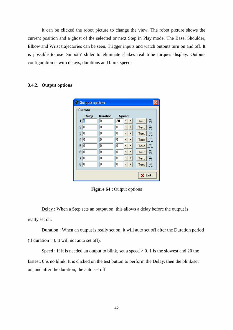
It is selected a Sequence in the Combo-box, and is clicked on the 'plus sign' to append,

or on the 'right arrow and the little plus sign' to insert. To delete a sequence (from list only), it

is selected a sequence in the list and is clicked on the 'left arrow with a minus sign'. It is

possible to delete only sequence with the delete icon, not the structures words. The Sequence

list contains Sequences from one Project only.

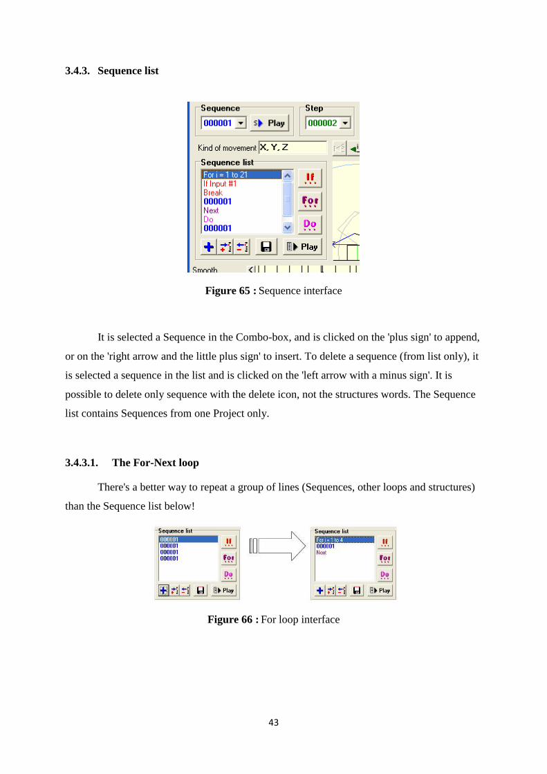
3.4.3.1. The For-Next loop

There's a better way to repeat a group of lines (Sequences, other loops and structures)

than the Sequence list below!

Figure 66 : For loop interface

44

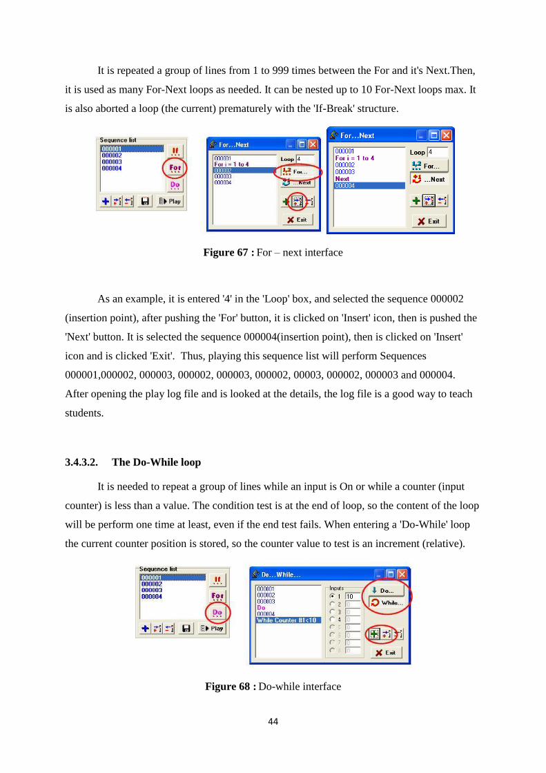
It is repeated a group of lines from 1 to 999 times between the For and it's Next.Then,

it is used as many For-Next loops as needed. It can be nested up to 10 For-Next loops max. It

is also aborted a loop (the current) prematurely with the 'If-Break' structure.

Figure 67 : For – next interface

As an example, it is entered '4' in the 'Loop' box, and selected the sequence 000002

(insertion point), after pushing the 'For' button, it is clicked on 'Insert' icon, then is pushed the

'Next' button. It is selected the sequence 000004(insertion point), then is clicked on 'Insert'

icon and is clicked 'Exit'. Thus, playing this sequence list will perform Sequences

000001,000002, 000003, 000002, 000003, 000002, 00003, 000002, 000003 and 000004.

After opening the play log file and is looked at the details, the log file is a good way to teach

students.

3.4.3.2. The Do-While loop

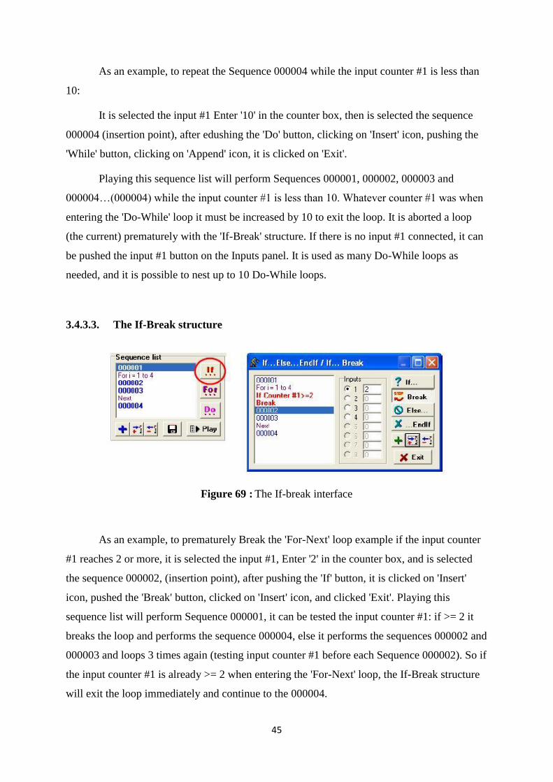
It is needed to repeat a group of lines while an input is On or while a counter (input

counter) is less than a value. The condition test is at the end of loop, so the content of the loop

will be perform one time at least, even if the end test fails. When entering a 'Do-While' loop

the current counter position is stored, so the counter value to test is an increment (relative).

Figure 68 : Do-while interface

45

As an example, to repeat the Sequence 000004 while the input counter #1 is less than

10:

It is selected the input #1 Enter '10' in the counter box, then is selected the sequence

000004 (insertion point), after edushing the 'Do' button, clicking on 'Insert' icon, pushing the

'While' button, clicking on 'Append' icon, it is clicked on 'Exit'.

Playing this sequence list will perform Sequences 000001, 000002, 000003 and

000004…(000004) while the input counter #1 is less than 10. Whatever counter #1 was when

entering the 'Do-While' loop it must be increased by 10 to exit the loop. It is aborted a loop

(the current) prematurely with the 'If-Break' structure. If there is no input #1 connected, it can

be pushed the input #1 button on the Inputs panel. It is used as many Do-While loops as

needed, and it is possible to nest up to 10 Do-While loops.

3.4.3.3. The If-Break structure

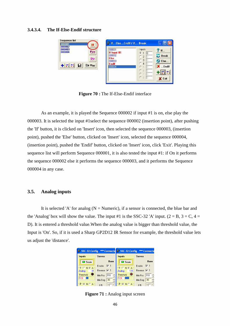
Figure 69 : The If-break interface

As an example, to prematurely Break the 'For-Next' loop example if the input counter

#1 reaches 2 or more, it is selected the input #1, Enter '2' in the counter box, and is selected

the sequence 000002, (insertion point), after pushing the 'If' button, it is clicked on 'Insert'

icon, pushed the 'Break' button, clicked on 'Insert' icon, and clicked 'Exit'. Playing this

sequence list will perform Sequence 000001, it can be tested the input counter #1: if >= 2 it

breaks the loop and performs the sequence 000004, else it performs the sequences 000002 and

000003 and loops 3 times again (testing input counter #1 before each Sequence 000002). So if

the input counter #1 is already >= 2 when entering the 'For-Next' loop, the If-Break structure

will exit the loop immediately and continue to the 000004.

46

3.4.3.4. The If-Else-Endif structure

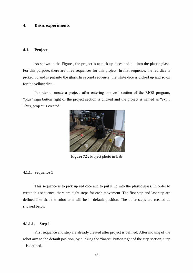
Figure 70 : The If-Else-Endif interface

As an example, it is played the Sequence 000002 if input #1 is on, else play the

000003. It is selected the input #1select the sequence 000002 (insertion point), after pushing

the 'If' button, it is clicked on 'Insert' icon, then selected the sequence 000003, (insertion

point), pushed the 'Else' button, clicked on 'Insert' icon, selected the sequence 000004,

(insertion point), pushed the 'Endif' button, clicked on 'Insert' icon, click 'Exit'. Playing this

sequence list will perform Sequence 000001, it is also tested the input #1: if On it performs

the sequence 000002 else it performs the sequence 000003, and it performs the Sequence

000004 in any case.

3.5. Analog inputs

It is selected 'A' for analog (N = Numeric), if a sensor is connected, the blue bar and

the 'Analog' box will show the value. The input #1 is the SSC-32 'A' input. (2 = B, 3 = C, 4 =

D). It is entered a threshold value.When the analog value is bigger than threshold value, the

Input is 'On'. So, if it is used a Sharp GP2D12 IR Sensor for example, the threshold value lets

us adjust the 'distance'.

Figure 71 : Analog input screen

47

This can also be tried:

* It is gone to the 'Moves' module and selected 'Demo 01 XYZ'.

* Then, it is selected sequence 000001 and after step 000001, and selected inputs #1.

* It will select 'Wait for' as default 'input action', it can changed the threshold value if

needed.

* Then, by going to the 'Play' module and is clicked on the Project Play button.

* The Program will wait until the analog input #1 > threshold value.

* If it is used a Sharp GP2D12 IR Sensor for example, just the sensor is approached

with your hand and the program will start!

48

4. Basic experiments

4.1. Project

As shown in the Figure , the project is to pick up dices and put into the plastic glass.

For this purpose, there are three sequences for this project. In first sequence, the red dice is

picked up and is put into the glass. In second sequence, the white dice is picked up and so on

for the yellow dice.

In order to create a project, after entering “moves” section of the RIOS program,

“plus” sign button right of the project section is clicked and the project is named as “exp”.

Thus, project is created.

Figure 72 : Project photo in Lab

4.1.1. Sequence 1

This sequence is to pick up red dice and to put it up into the plastic glass. In order to

create this sequence, there are eight steps for each movement. The first step and last step are

defined like that the robot arm will be in default position. The other steps are created as

showed below.

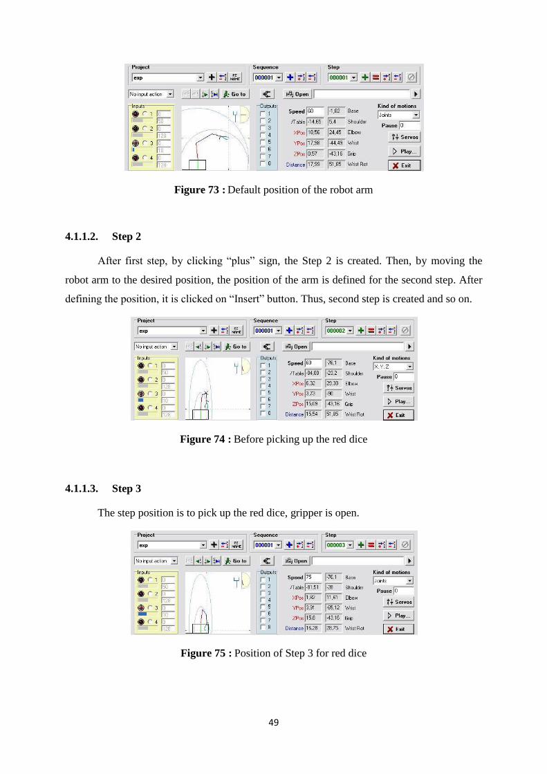
4.1.1.1. Step 1

First sequence and step are already created after project is defined. After moving of the

robot arm to the default position, by clicking the “insert” button right of the step section, Step

1 is defined.

49

Figure 73 : Default position of the robot arm

4.1.1.2. Step 2

After first step, by clicking “plus” sign, the Step 2 is created. Then, by moving the

robot arm to the desired position, the position of the arm is defined for the second step. After

defining the position, it is clicked on “Insert” button. Thus, second step is created and so on.

Figure 74 : Before picking up the red dice

4.1.1.3. Step 3

The step position is to pick up the red dice, gripper is open.

Figure 75 : Position of Step 3 for red dice

50

4.1.1.4. Step 4

The step position is to pick up the red dice, gripper is closed.The red dice is picked up.


4.1.1.5. Step 5

The robot arm is positioned slightly before putting of red dice into the plastic glass.


4.1.1.6. Step 6

The robot arm is positioned on putting of red dice into the plastic glass, the gripper is

still closed.


51

4.1.1.7. Step 7

The robot arm is positioned on putting of red dice into the plastic glass, the gripper is

opened and red dice is fallen down into the plastic glass.


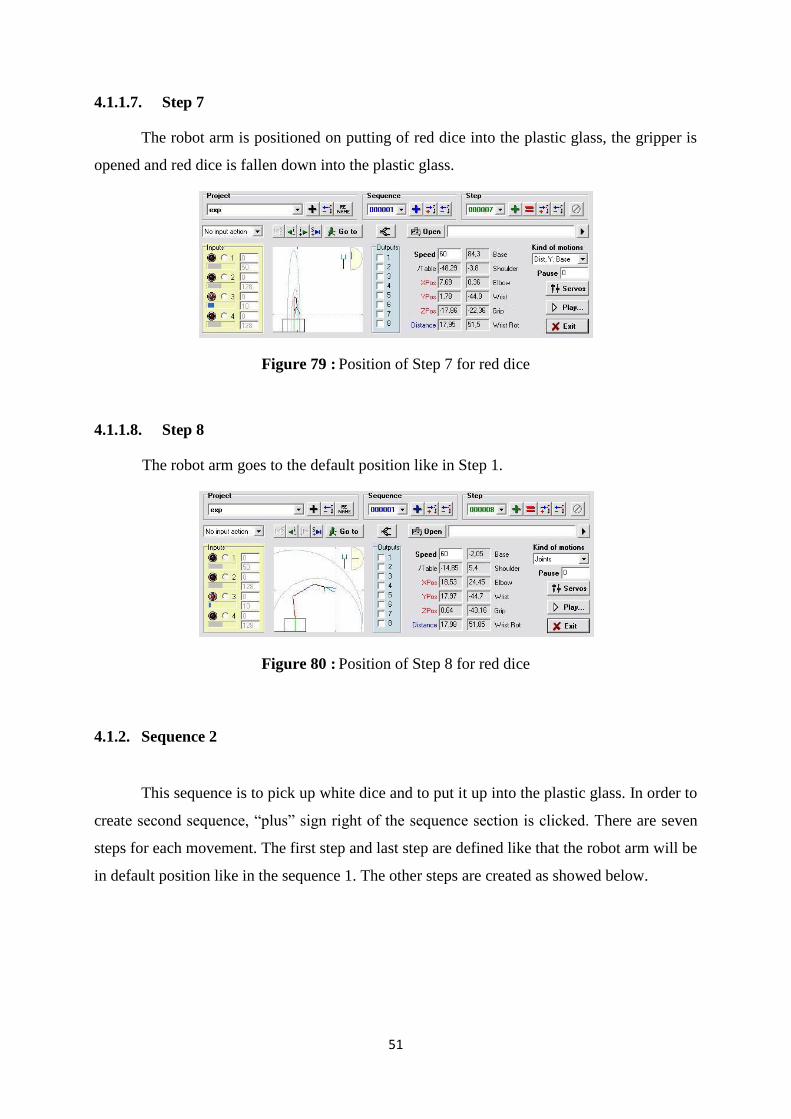
4.1.1.8. Step 8

The robot arm goes to the default position like in Step 1.


4.1.2. Sequence 2

This sequence is to pick up white dice and to put it up into the plastic glass. In order to

create second sequence, “plus” sign right of the sequence section is clicked. There are seven

steps for each movement. The first step and last step are defined like that the robot arm will be

in default position like in the sequence 1. The other steps are created as showed below.

52

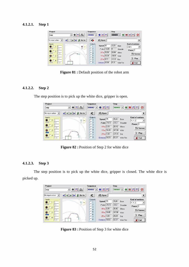
4.1.2.1. Step 1

Figure 81 : Default position of the robot arm

4.1.2.2. Step 2

The step position is to pick up the white dice, gripper is open.

Figure 82 : Position of Step 2 for white dice

4.1.2.3. Step 3

The step position is to pick up the white dice, gripper is closed. The white dice is

picked up.


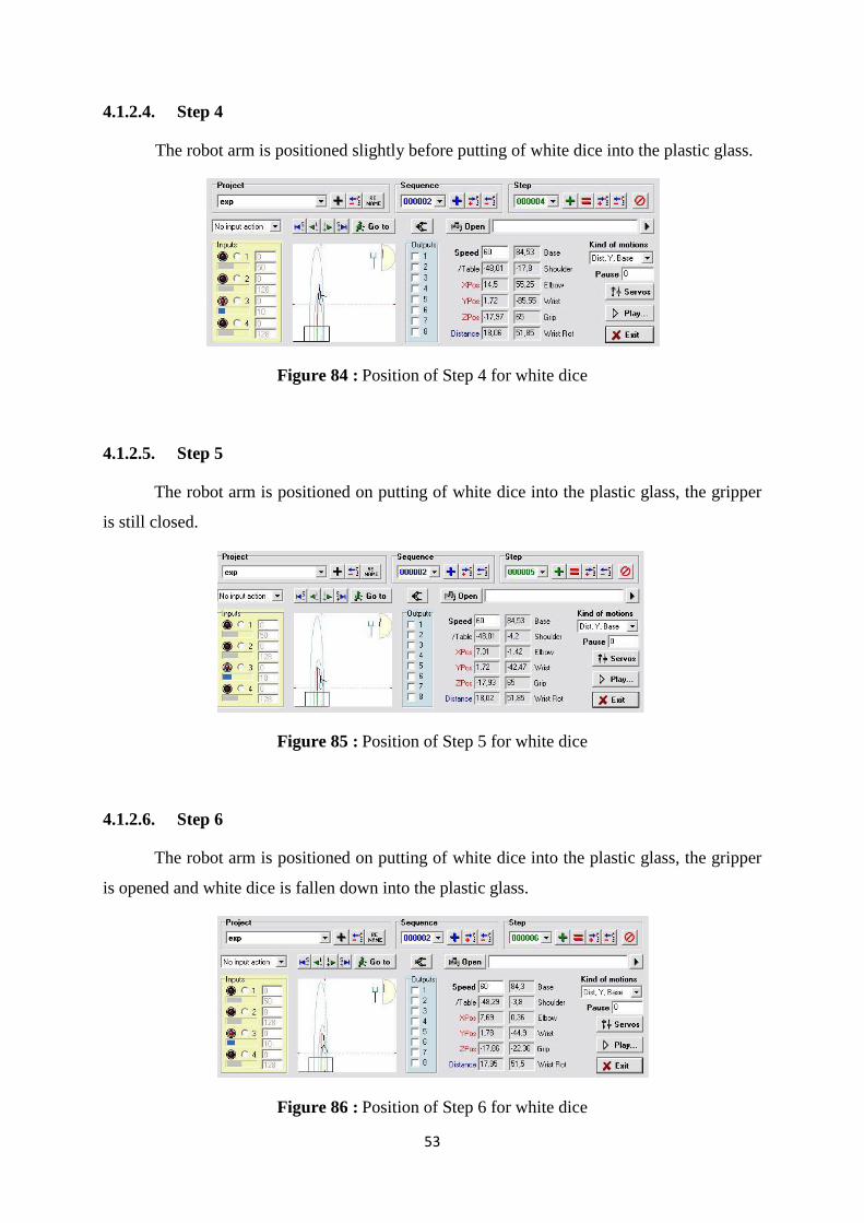
53

4.1.2.4. Step 4

The robot arm is positioned slightly before putting of white dice into the plastic glass.


4.1.2.5. Step 5

The robot arm is positioned on putting of white dice into the plastic glass, the gripper

is still closed.


4.1.2.6. Step 6

The robot arm is positioned on putting of white dice into the plastic glass, the gripper

is opened and white dice is fallen down into the plastic glass.


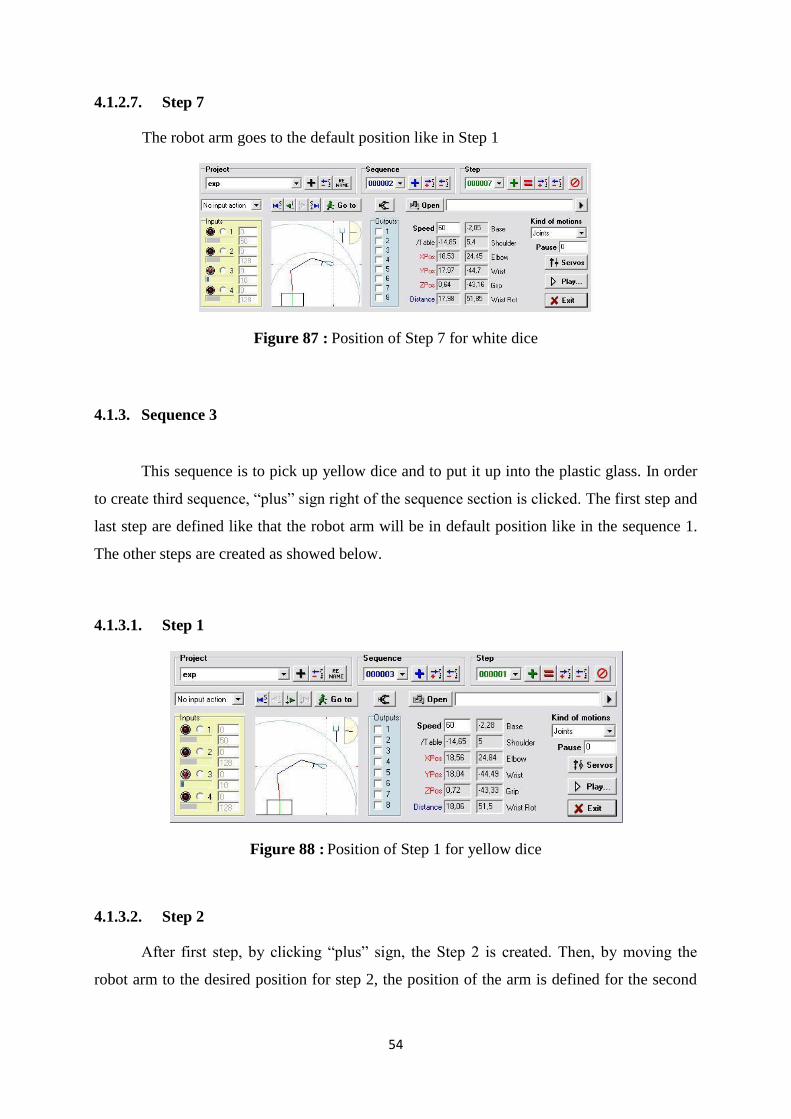
54

4.1.2.7. Step 7

The robot arm goes to the default position like in Step 1


4.1.3. Sequence 3

This sequence is to pick up yellow dice and to put it up into the plastic glass. In order

to create third sequence, “plus” sign right of the sequence section is clicked. The first step and

last step are defined like that the robot arm will be in default position like in the sequence 1.

The other steps are created as showed below.

4.1.3.1. Step 1

Figure 88 : Position of Step 1 for yellow dice

4.1.3.2. Step 2

After first step, by clicking “plus” sign, the Step 2 is created. Then, by moving the

robot arm to the desired position for step 2, the position of the arm is defined for the second

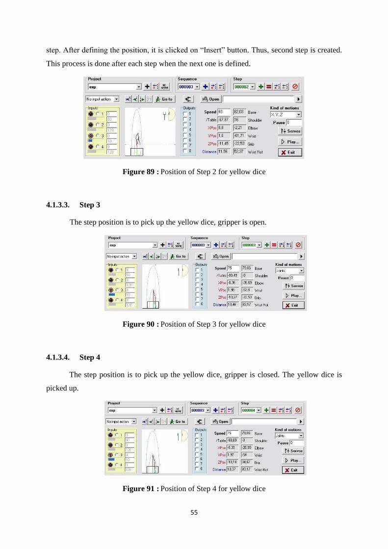
55

step. After defining the position, it is clicked on “Insert” button. Thus, second step is created.

This process is done after each step when the next one is defined.


4.1.3.3. Step 3

The step position is to pick up the yellow dice, gripper is open.


4.1.3.4. Step 4

The step position is to pick up the yellow dice, gripper is closed. The yellow dice is

picked up.


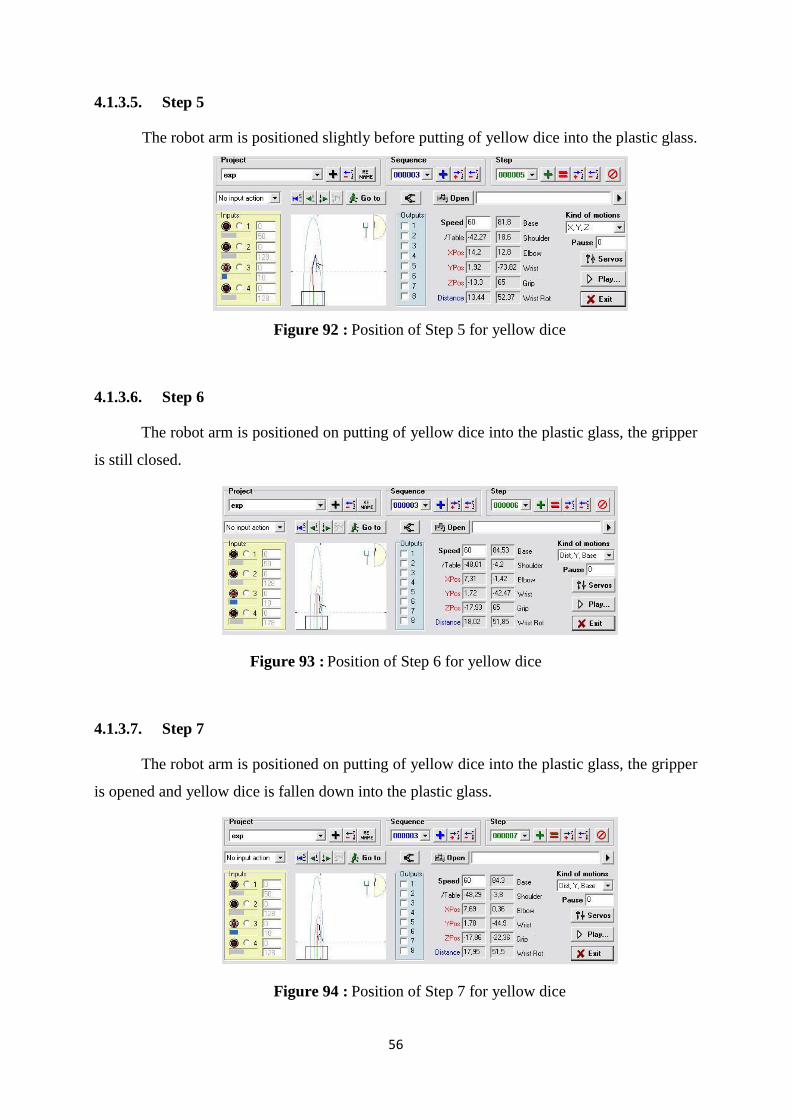
56

4.1.3.5. Step 5

The robot arm is positioned slightly before putting of yellow dice into the plastic glass.


4.1.3.6. Step 6

The robot arm is positioned on putting of yellow dice into the plastic glass, the gripper

is still closed.


4.1.3.7. Step 7

The robot arm is positioned on putting of yellow dice into the plastic glass, the gripper

is opened and yellow dice is fallen down into the plastic glass.


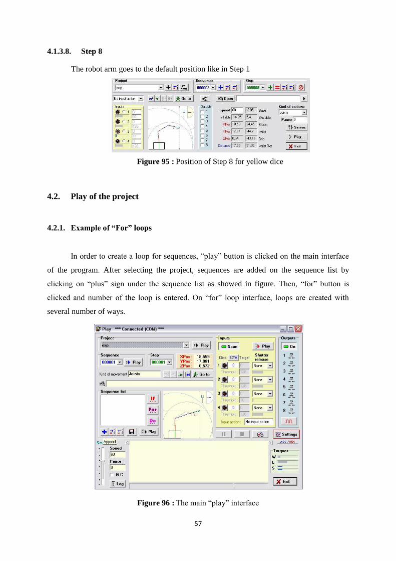
57

4.1.3.8. Step 8

The robot arm goes to the default position like in Step 1


4.2. Play of the project

4.2.1. Example of “For” loops

In order to create a loop for sequences, “play” button is clicked on the main interface

of the program. After selecting the project, sequences are added on the sequence list by

clicking on “plus” sign under the sequence list as showed in figure. Then, “for” button is

clicked and number of the loop is entered. On “for” loop interface, loops are created with

several number of ways.

Figure 96 : The main “play” interface

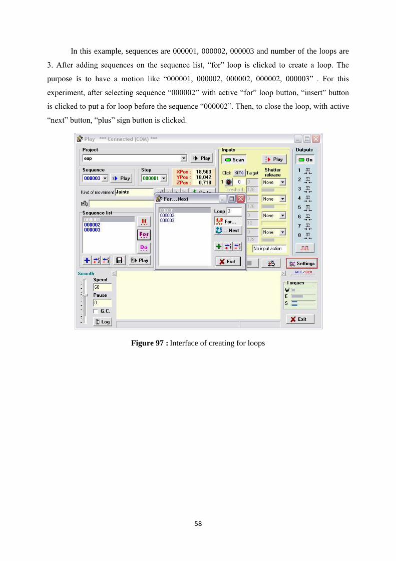
58

In this example, sequences are 000001, 000002, 000003 and number of the loops are

3. After adding sequences on the sequence list, “for” loop is clicked to create a loop. The

purpose is to have a motion like “000001, 000002, 000002, 000002, 000003” . For this

experiment, after selecting sequence “000002” with active “for” loop button, “insert” button

is clicked to put a for loop before the sequence “000002”. Then, to close the loop, with active

“next” button, “plus” sign button is clicked.

Figure 97 : Interface of creating for loops

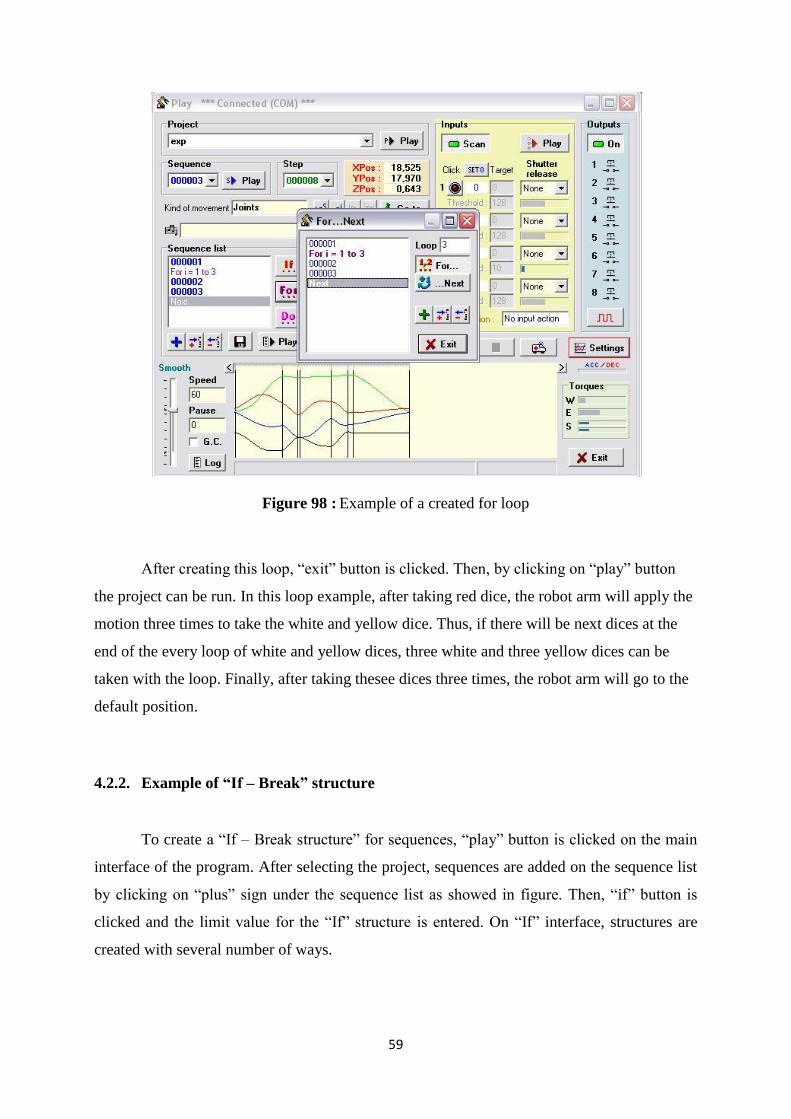
59

Figure 98 : Example of a created for loop

After creating this loop, “exit” button is clicked. Then, by clicking on “play” button

the project can be run. In this loop example, after taking red dice, the robot arm will apply the

motion three times to take the white and yellow dice. Thus, if there will be next dices at the

end of the every loop of white and yellow dices, three white and three yellow dices can be

taken with the loop. Finally, after taking thesee dices three times, the robot arm will go to the

default position.

4.2.2. Example of “If – Break” structure

To create a “If – Break structure” for sequences, “play” button is clicked on the main

interface of the program. After selecting the project, sequences are added on the sequence list

by clicking on “plus” sign under the sequence list as showed in figure. Then, “if” button is

clicked and the limit value for the “If” structure is entered. On “If” interface, structures are

created with several number of ways.

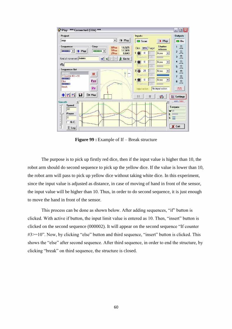
60

Figure 99 : Example of If – Break structure

The purpose is to pick up firstly red dice, then if the input value is higher than 10, the

robot arm should do second sequence to pick up the yellow dice. If the value is lower than 10,

the robot arm will pass to pick up yellow dice without taking white dice. In this experiment,

since the input value is adjusted as distance, in case of moving of hand in front of the sensor,

the input value will be higher than 10. Thus, in order to do second sequence, it is just enough

to move the hand in front of the sensor.

This process can be done as shown below. After adding sequences, “if” button is

clicked. With active if button, the input limit value is entered as 10. Then, “insert” button is

clicked on the second sequence (000002). It will appear on the second sequence “If counter

#3>=10”. Now, by clicking “else” button and third sequence, “insert” button is clicked. This

shows the “else” after second sequence. After third sequence, in order to end the structure, by

clicking “break” on third sequence, the structure is closed.

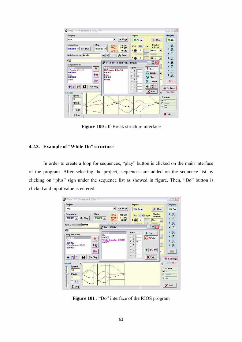
61

Figure 100 : If-Break structure interface

4.2.3. Example of “While-Do” structure

In order to create a loop for sequences, “play” button is clicked on the main interface

of the program. After selecting the project, sequences are added on the sequence list by

clicking on “plus” sign under the sequence list as showed in figure. Then, “Do” button is

clicked and input value is entered.

Figure 101 : “Do” interface of the RIOS program

62

In this example, input limit value is equal to 10. This means that the robot arm will do

firstly sequence “000001” . Then, it continues to do sequence “000002, while the input value

of the GP2D12 sensor is lower than 10. In case of passing this input value, for example,

moving of the hand in front of the sensor, the robot arm will do the next sequence “000003”.

Otherwise, that is, in case of having input value lower than 10, the robot arm will always

sequence “000002”. By this method, according to the distance values coming from the

GP2D12 sensor, several experiments can be done by writing simple commands in order to

show the capability of the robot in automation sector.

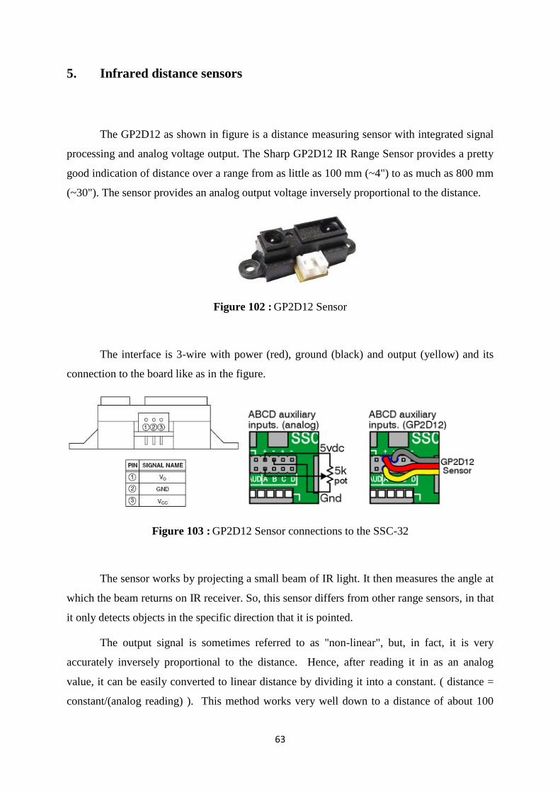
63

5. Infrared distance sensors

The GP2D12 as shown in figure is a distance measuring sensor with integrated signal

processing and analog voltage output. The Sharp GP2D12 IR Range Sensor provides a pretty

good indication of distance over a range from as little as 100 mm (~4") to as much as 800 mm

(~30"). The sensor provides an analog output voltage inversely proportional to the distance.

Figure 102 : GP2D12 Sensor

The interface is 3-wire with power (red), ground (black) and output (yellow) and its

connection to the board like as in the figure.

Figure 103 : GP2D12 Sensor connections to the SSC-32

The sensor works by projecting a small beam of IR light. It then measures the angle at

which the beam returns on IR receiver. So, this sensor differs from other range sensors, in that

it only detects objects in the specific direction that it is pointed.

The output signal is sometimes referred to as "non-linear", but, in fact, it is very

accurately inversely proportional to the distance. Hence, after reading it in as an analog

value, it can be easily converted to linear distance by dividing it into a constant. ( distance =

constant/(analog reading) ). This method works very well down to a distance of about 100

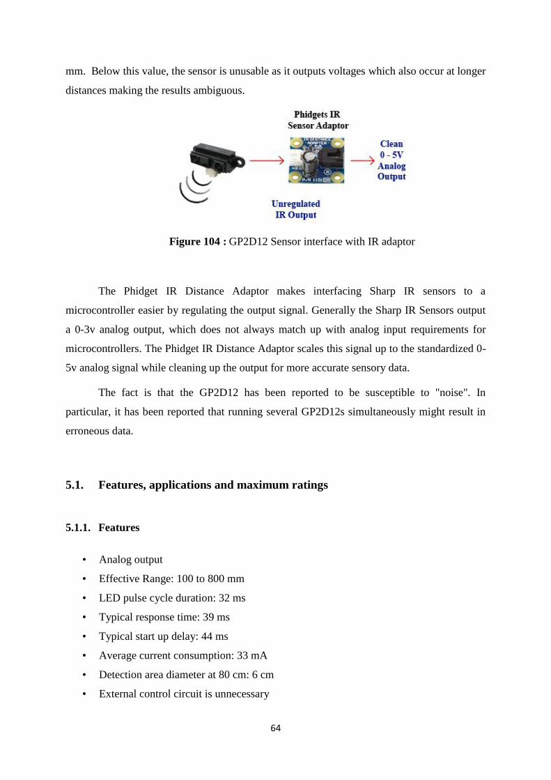
64

mm. Below this value, the sensor is unusable as it outputs voltages which also occur at longer

distances making the results ambiguous.

Figure 104 : GP2D12 Sensor interface with IR adaptor

The Phidget IR Distance Adaptor makes interfacing Sharp IR sensors to a

microcontroller easier by regulating the output signal. Generally the Sharp IR Sensors output

a 0-3v analog output, which does not always match up with analog input requirements for

microcontrollers. The Phidget IR Distance Adaptor scales this signal up to the standardized 0-

5v analog signal while cleaning up the output for more accurate sensory data.

The fact is that the GP2D12 has been reported to be susceptible to "noise". In

particular, it has been reported that running several GP2D12s simultaneously might result in

erroneous data.

5.1. Features, applications and maximum ratings

5.1.1. Features

• Analog output

• Effective Range: 100 to 800 mm

• LED pulse cycle duration: 32 ms

• Typical response time: 39 ms

• Typical start up delay: 44 ms

• Average current consumption: 33 mA

• Detection area diameter at 80 cm: 6 cm

• External control circuit is unnecessary

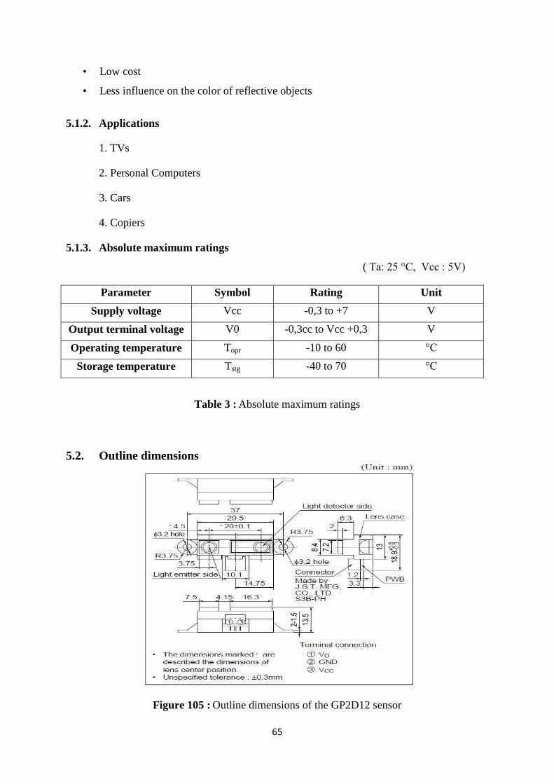
65

• Low cost

• Less influence on the color of reflective objects

5.1.2. Applications

1. TVs

2. Personal Computers

3. Cars

4. Copiers

5.1.3. Absolute maximum ratings

( Ta: 25 °C, Vcc : 5V)

Parameter Symbol Rating Unit

Supply voltage Vcc -0,3 to +7 V

Output terminal voltage V0 -0,3cc to Vcc +0,3 V

Operating temperature Topr -10 to 60 °C

Storage temperature Tstg -40 to 70 °C

Table 3 : Absolute maximum ratings

5.2. Outline dimensions

Figure 105 : Outline dimensions of the GP2D12 sensor

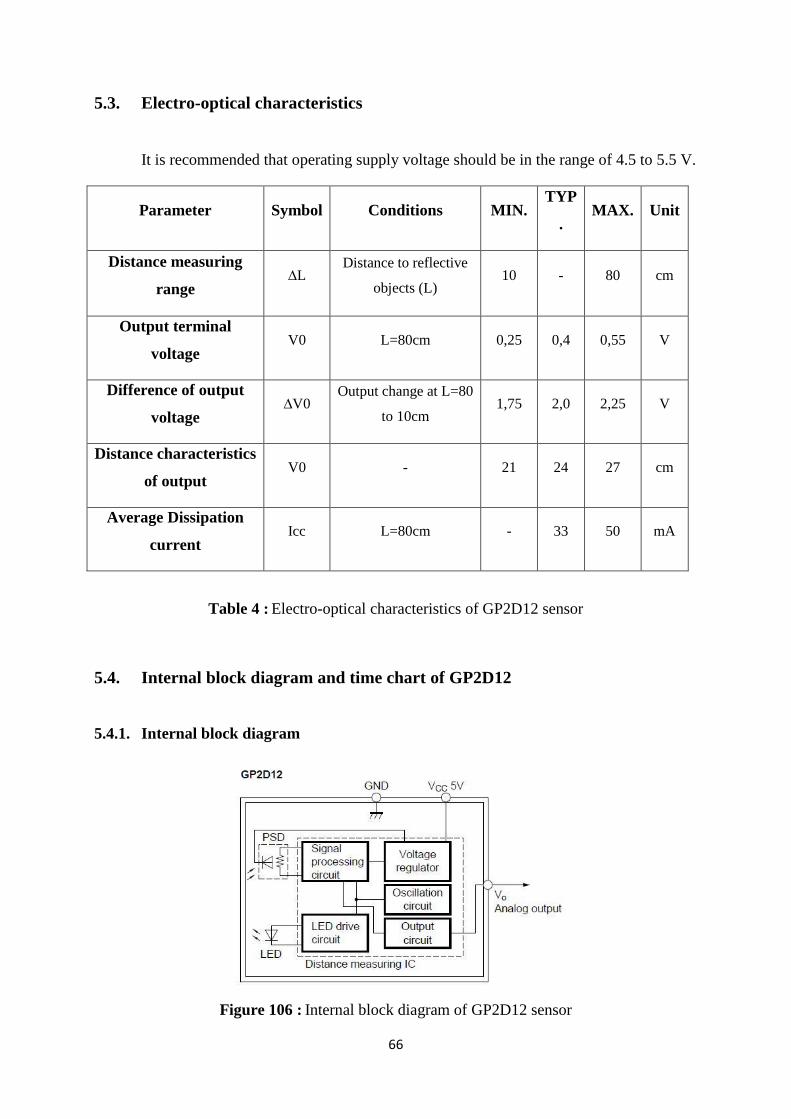
66

5.3. Electro-optical characteristics

It is recommended that operating supply voltage should be in the range of 4.5 to 5.5 V.

Parameter Symbol Conditions MIN. TYP

. MAX. Unit

Distance measuring

range ∆L

Distance to reflective

objects (L) 10 - 80 cm

Output terminal

voltage V0 L=80cm 0,25 0,4 0,55 V

Difference of output

voltage ∆V0

Output change at L=80

to 10cm 1,75 2,0 2,25 V

Distance characteristics

of output V0 - 21 24 27 cm

Average Dissipation

current Icc L=80cm - 33 50 mA

Table 4 : Electro-optical characteristics of GP2D12 sensor

5.4. Internal block diagram and time chart of GP2D12

5.4.1. Internal block diagram

Figure 106 : Internal block diagram of GP2D12 sensor

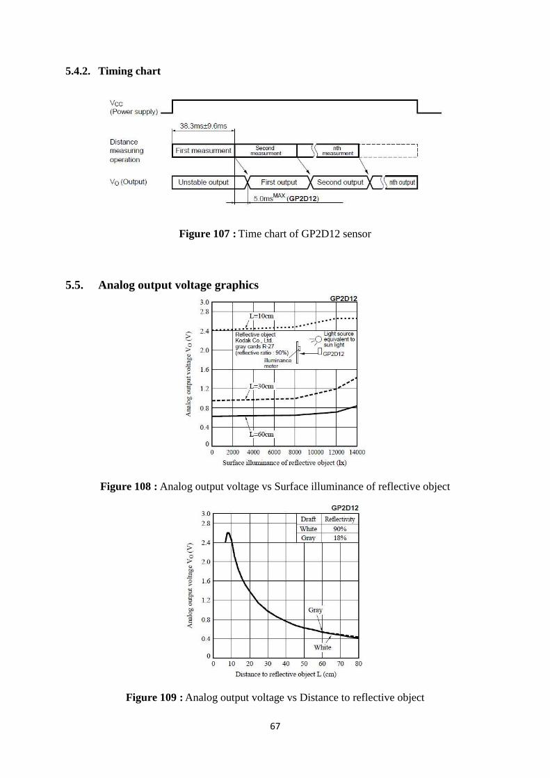
67

5.4.2. Timing chart

Figure 107 : Time chart of GP2D12 sensor

5.5. Analog output voltage graphics

Figure 108 : Analog output voltage vs Surface illuminance of reflective object

Figure 109 : Analog output voltage vs Distance to reflective object

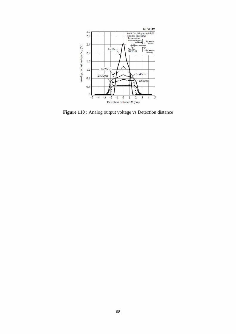
68

Figure 110 : Analog output voltage vs Detection distance

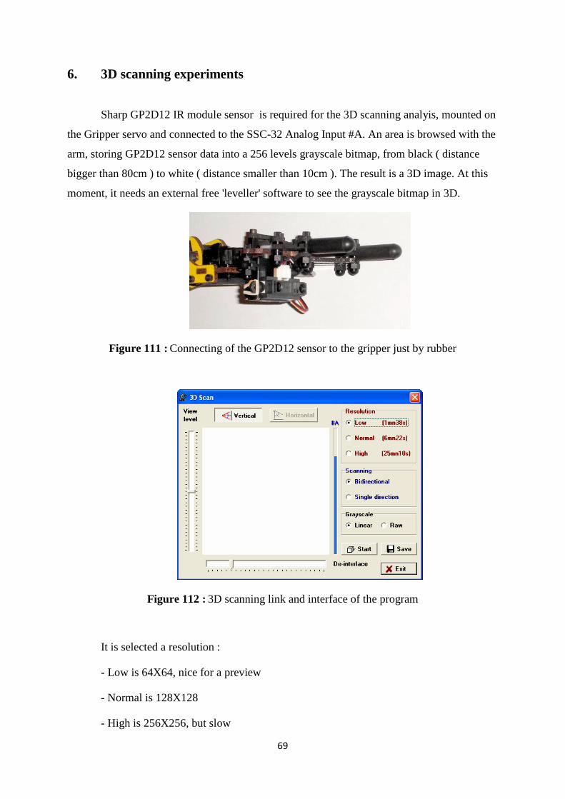
69

6. 3D scanning experiments

Sharp GP2D12 IR module sensor is required for the 3D scanning analyis, mounted on

the Gripper servo and connected to the SSC-32 Analog Input #A. An area is browsed with the

arm, storing GP2D12 sensor data into a 256 levels grayscale bitmap, from black ( distance

bigger than 80cm ) to white ( distance smaller than 10cm ). The result is a 3D image. At this

moment, it needs an external free 'leveller' software to see the grayscale bitmap in 3D.

Figure 111 : Connecting of the GP2D12 sensor to the gripper just by rubber

Figure 112 : 3D scanning link and interface of the program

It is selected a resolution :

- Low is 64X64, nice for a preview

- Normal is 128X128

- High is 256X256, but slow

70

It is selected scanning direction :

- Bidirectional is fast but not the best quality.

- Single direction is a bit slower but pretty good result.

It is pressed 'Start' to begin the Scan. In order to understand the sliders, it is import to

point out of physical explanations of the parameters below.

Grayscale :

- Linear option means that datas from the GP2D12 are corrected to be proportionally

spaced, according to the distance (correcting the non-linearity of the GP2D12).

- Raw option means that datas are only scaled to suit the 0-255 grayscale range.

There is no obligatory to choose the grayscale option before starting the scan. It is

possible to change this after the scan is complete to decide the one it will be saved, or it is

possible to select 'linear', save it as bmp image, then select 'raw' and save it too. This option

can be changed during the scanning process too, just to checking now.

De-interlace :

This slider allows fine adjustment to the odd and even lines matching. It's very useful

when using the bidirectional scanning option. For single direction scanning, set the slider in

the middle. This setting can be changed during the scanning process or after it's complete.

View level : (This is used when the scanning process is complete)

This can be used in two different ways :

- It is move the slider slowly to highlight in red the corresponding level (distance). It's

useful to see all the pixels on the 'same level'.

- It is clicked on the bitmap (left click) and keep pressed, then move the mouse cursor

on the bitmap, all the 'same level' pixels as the one hovering are highlighted in red, and the

view level slider reflects the current level.

Save :

It is saved the current scan to a 256X256 grayscale bitmap (*.bmp) file. It doesn't save

any red pixel from the 'view level' feature.

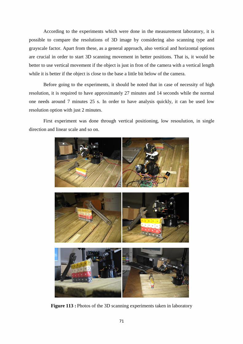
71

According to the experiments which were done in the measurement laboratory, it is

possible to compare the resolutions of 3D image by considering also scanning type and

grayscale factor. Apart from these, as a general approach, also vertical and horizontal options

are crucial in order to start 3D scanning movement in better positions. That is, it would be

better to use vertical movement if the object is just in fron of the camera with a vertical length

while it is better if the object is close to the base a little bit below of the camera.

Before going to the experiments, it should be noted that in case of necessity of high

resolution, it is required to have approximately 27 minutes and 14 seconds while the normal

one needs around 7 minutes 25 s. In order to have analysis quickly, it can be used low

resolution option with just 2 minutes.

First experiment was done through vertical positioning, low resoulution, in single

direction and linear scale and so on.

Figure 113 : Photos of the 3D scanning experiments taken in laboratory

72

Figure 114 : Vertical, low resolution, single direction, linear

Figure 115 : Vertical, low resolution, bidirectional, linear

Figure 116 : Vertical, low resolution, single direction, raw

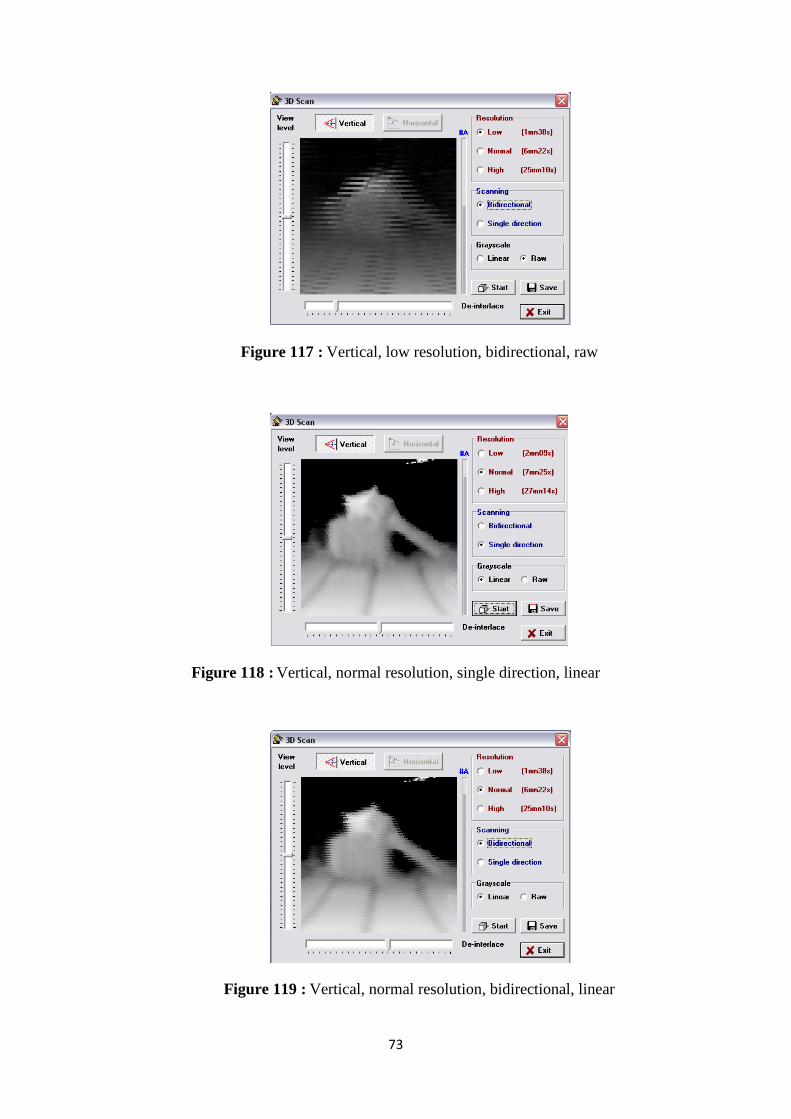
73

Figure 117 : Vertical, low resolution, bidirectional, raw

Figure 118 : Vertical, normal resolution, single direction, linear

Figure 119 : Vertical, normal resolution, bidirectional, linear

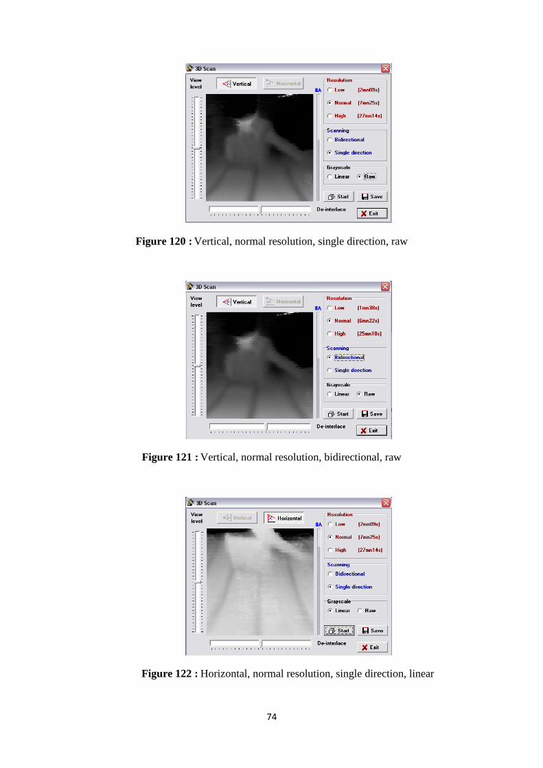
74

Figure 120 : Vertical, normal resolution, single direction, raw

Figure 121 : Vertical, normal resolution, bidirectional, raw

Figure 122 : Horizontal, normal resolution, single direction, linear

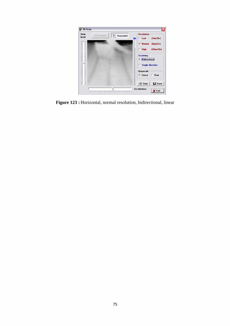
75

Figure 123 : Horizontal, normal resolution, bidirectional, linear

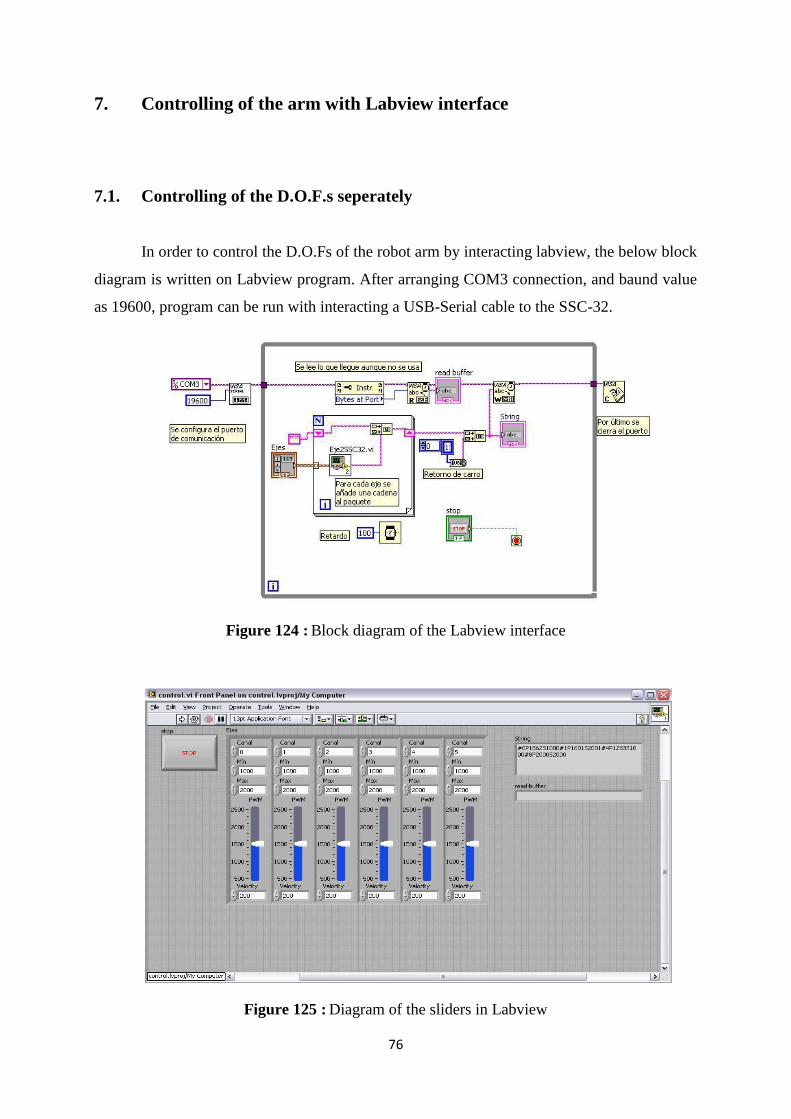
76

7. Controlling of the arm with Labview interface

7.1. Controlling of the D.O.F.s seperately

In order to control the D.O.Fs of the robot arm by interacting labview, the below block

diagram is written on Labview program. After arranging COM3 connection, and baund value

as 19600, program can be run with interacting a USB-Serial cable to the SSC-32.

Figure 124 : Block diagram of the Labview interface

Figure 125 : Diagram of the sliders in Labview

77

After running program, the servomotors of the robot arm can be controlled by the

sliders which are created according to number of the DOFs. On the bottom of the sliders,

velocity of the movement can be set to desired value. By moving the robot arm DOFs

seperately, it is enough to move the slider. Maximum and minumum Pulse Width

Module(PWM) can be rearranged accordint to the desired limit positions of the robot arm for

each DOF.

7.2. Robot identification in Labview

7.2.1. Introduction to kinematic analysis for Labview

Robot arms have n-links that are connected together by joints. For movement of these

joints, each motor combined its own joint gives the motion to the commanded link. The

outputs like position, velocity and torque are measured by feedback sensors which are

connected to the motors. Links and joints form a kinematic chain connected to ground from

previous side to the next side. For handling materials or welding or to do some tasks like

these, the end-effector (e.g. gripper, welding tool, or another tool) is placed at the end of the

open side. The number of the DOF, which refers to the number of joints, leads to name of the

robot manipulator For example, if robot arm has 5 joints, it means the robot has 5DOF, and so

on. In industrial and practical applications, the position of the end effector of the robot must

be defined in a global coordinate system. In order to convert of the coordinate systems, the

coordinates of the end effector from the local position to the global position, the robot

movements are represented by a series of movements of rigid links. Each link sets a proper

transformation matrix regarding the position of the current link to the previous link. As

mentioned previously, robot manipulator whose all joints are prismatic is known as a

cartesian manipulator while the robot whose joint variables are revolute is called an

articulated manipulator.

Kinematics is referred to motion geometry of the robot arm which starts from the

reference position to the desired position by ignoring the forces or other factors that effect

robot motion. Namely, the kinematics are created by the movement of the robot arm in

comparison to fixed frame as a function of time. The fixed frame shows the base and all other

movements measured from the base as reference. This is the most crucial disciplines in

78

robots, providing tools in order to define the structure and acts of robot arm mechanisms, and

it is vital in practical applications like control purposes and planning of the trajectory.

7.2.2. Denavit – Hertanberg (DH) parameters

Usually, kinematic analysis and its desription is so significant in order to control any

core of controller design of the robot arm. In industrial and academic field, this is done by

applying a common method, that is Denavit-Hartenberg method. A mathematical definining

for all serial arms depending on the robot geometry is taken by the distinct of this method, and

it defines the position and orientation of the current link in comparison to previous link.

Furthermore, it allows the desired frame to create a set of steps to bring the other links

coordinate into corresponding with another one. The kinematic solution in this chapter will

focus on two important problem arises in robot manipulator. Section (2.2) discusses

methodologies to solve the forward and inverse kinematic respectively.

The first problem is how to determine the forward kinematic (FK) where the robot arm

end-effector will take place if all joints are already known. This means what rigid motion each

joint effect on its link to obtain the desired configuration. The configuration space of the end-

effector contains the transformation matrix T that relates the position and orientation of the

end-effector. The following equation explains the forward kinematic problem.

F(θ1, θ2, ..., θn) = [x, y, z, Rd ]

where θ1, θ2 , and θn are the input variables, [x, y, z] are the desired position and Rd the

desired rotation.

The second problem is determining the inverse kinematic (IK), which calculates the

value of each joint variable if the desired position and orientation of end-effector are known.

That means if the final link configuration is known, what is the possible configuration (e.g.

solutions) of the robot manipulator to move the end effector of the robot arm to desired

position and orientation in space. Inverse kinematic problem may express mathematically as

follows:

F(x, y, z, Rd) = [θ1, θ2, ..., θn]

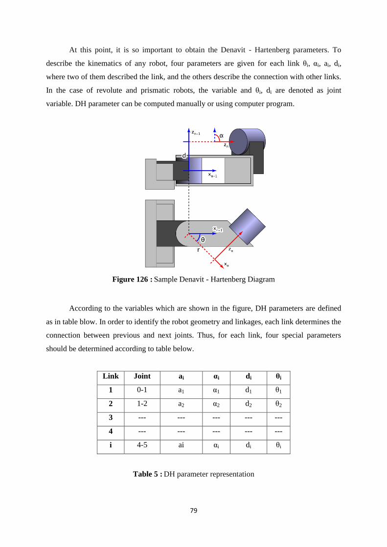
79

At this point, it is so important to obtain the Denavit - Hartenberg parameters. To

describe the kinematics of any robot, four parameters are given for each link θi, αi, ai, di,

where two of them described the link, and the others describe the connection with other links.

In the case of revolute and prismatic robots, the variable and θi, di are denoted as joint

variable. DH parameter can be computed manually or using computer program.

Figure 126 : Sample Denavit - Hartenberg Diagram

According to the variables which are shown in the figure, DH parameters are defined

as in table blow. In order to identify the robot geometry and linkages, each link determines the

connection between previous and next joints. Thus, for each link, four special parameters

should be determined according to table below.

Link Joint ai αi di θi

1 0-1 a1 α1 d1 θ1

2 1-2 a2 α2 d2 θ2

3 --- --- --- --- ---

4 --- --- --- --- ---

i 4-5 ai αi di θi

Table 5 : DH parameter representation

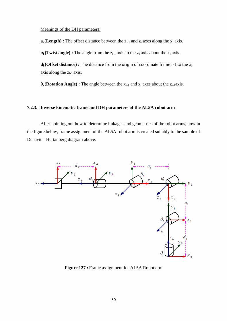
80

Meanings of the DH parameters:

ai (Length) : The offset distance between the zi-1 and zi axes along the xi axis.

αi (Twist angle) : The angle from the zi-1 axis to the zi axis about the xi axis.

di (Offset distance) : The distance from the origin of coordinate frame i-1 to the xi

axis along the zi-1 axis.

θi (Rotation Angle) : The angle between the xi-1 and xi axes about the zi-1axis.

7.2.3. Inverse kinematic frame and DH parameters of the AL5A robot arm

After pointing out how to determine linkages and geometries of the robot arms, now in

the figure below, frame assignment of the AL5A robot arm is created suitably to the sample of

Denavit – Hertanberg diagram above.

Figure 127 : Frame assignment for AL5A Robot arm

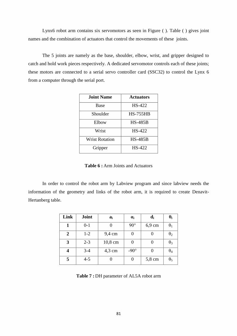
81

Lynx6 robot arm contains six servomotors as seen in Figure ( ). Table ( ) gives joint

names and the combination of actuators that control the movements of these joints.

The 5 joints are namely as the base, shoulder, elbow, wrist, and gripper designed to

catch and hold work pieces respectively. A dedicated servomotor controls each of these joints;

these motors are connected to a serial servo controller card (SSC32) to control the Lynx 6

from a computer through the serial port.

Joint Name Actuators

Base HS-422

Shoulder HS-755HB

Elbow HS-485B

Wrist HS-422

Wrist Rotation HS-485B

Gripper HS-422

Table 6 : Arm Joints and Actuators

In order to control the robot arm by Labview program and since labview needs the

information of the geometry and links of the robot arm, it is required to create Denavit-

Hertanberg table.

Link Joint ai αi di θi

1 0-1 0 90° 6,9 cm θ1

2 1-2 9,4 cm 0 0 θ2

3 2-3 10,8 cm 0 0 θ3

4 3-4 4,3 cm -90° 0 θ4

5 4-5 0 0 5,8 cm θ5

Table 7 : DH parameter of AL5A robot arm

82

8. Conclusion and future aspects

In conclusion, after assembly and calibration of the AL5A robot arm, some basic

movements and experiments can be created through using the RIOS program in PC

environment. By exporting the files as .csv format, and then by editing the positions, desired

motion of the robot can be imported again on the program in order to move the robot in

desired way. Besides of this movements and experiments, also 3D scanning interface of the

program can get the 3D images by the GP2D12 sensor which is mounted on the gripper. As

seen in last part of the thesis, on labview interface, some basic codes can be written in order to

move the servos of the robot.

In the future, by developing the codes which were written in Labview, it would be

possible to move the robot arm with a web-camera that is mounted on the gripper. According

to the image acquisitions from web camera, the robot can follow the positions which are

programmed in Labview environment. By this method, some approaches can be investigated

with the purpose of their usage on the industrial automation sector.

83

9. References

[1] B. Koyuncu and M. Güzel, “Software Development for the Kinematic Analysis of a

Lynx 6 Robot Arm,” Proceedings of World Academy of Science, Engineering and

Technology., Oct. 2007.

[2] http://www.lynxmotion.com/driver.aspx?Topic=assem01

[3] Ahmed Zakari Alassar, “A Thesis in Modeling and Control of 5DOF Robot Arm Using

Supervisory Control”, The Islamic University of Gaza, March 2010

[4] The Tech Museum of Innovation, "Robotics: About the Exhibition", Sep. 2009.

[5] Kurt E. Clothier and Ying Shang, “A Geometric Approach for Robotic Arm

Kinematics with Hardware Design, Electrical Design, and Implementation”, Department

of Electrical & Computer Engineering, Southern Illinois University Edwardsville, 18 August

2010

[6] http://www.osha.gov/dts/osta/otm/otm_iv/otm_iv_4.html#2

[7] http://prime.jsc.nasa.gov/ROV/types.html

http://www.lynxmotion.com/driver.aspx?Topic=assem01

http://www.osha.gov/dts/osta/otm/otm_iv/otm_iv_4.html#2

laboratory experiences and 3d measurements with … · laboratory experiences and 3d measurements...

Documents