NREL is a national laboratory of the U.S. Department of Energy, Office of Energy Efficiency & Renewable Energy, operated by the Alliance for Sustainable Energy, LLC.

Contract No. DE-AC36-08GO28308

Investigating the Correlation Between Wind and Solar Power Forecast Errors in the Western Interconnection Preprint J. Zhang, B-M. Hodge, and A. Florita To be presented at the ASME 7th International Conference on Energy Sustainability and the 11th Fuel Cell Science, Engineering, and Technology Conference Minneapolis, Minnesota July 14–19, 2013

Conference Paper NREL/CP-5500-57816 May 2013

NOTICE

The submitted manuscript has been offered by an employee of the Alliance for Sustainable Energy, LLC (Alliance), a contractor of the US Government under Contract No. DE-AC36-08GO28308. Accordingly, the US Government and Alliance retain a nonexclusive royalty-free license to publish or reproduce the published form of this contribution, or allow others to do so, for US Government purposes.

This report was prepared as an account of work sponsored by an agency of the United States government. Neither the United States government nor any agency thereof, nor any of their employees, makes any warranty, express or implied, or assumes any legal liability or responsibility for the accuracy, completeness, or usefulness of any information, apparatus, product, or process disclosed, or represents that its use would not infringe privately owned rights. Reference herein to any specific commercial product, process, or service by trade name, trademark, manufacturer, or otherwise does not necessarily constitute or imply its endorsement, recommendation, or favoring by the United States government or any agency thereof. The views and opinions of authors expressed herein do not necessarily state or reflect those of the United States government or any agency thereof.

Available electronically at http://www.osti.gov/bridge

Available for a processing fee to U.S. Department of Energy and its contractors, in paper, from:

U.S. Department of Energy Office of Scientific and Technical Information P.O. Box 62 Oak Ridge, TN 37831-0062 phone: 865.576.8401 fax: 865.576.5728 email: mailto:reports@adonis.osti.gov

Available for sale to the public, in paper, from:

U.S. Department of Commerce National Technical Information Service 5285 Port Royal Road Springfield, VA 22161 phone: 800.553.6847 fax: 703.605.6900 email: orders@ntis.fedworld.gov online ordering: http://www.ntis.gov/help/ordermethods.aspx

Cover Photos: (left to right) PIX 16416, PIX 17423, PIX 16560, PIX 17613, PIX 17436, PIX 17721

Printed on paper containing at least 50% wastepaper, including 10% post consumer waste.

1

ESFuelCell2013-18423

INVESTIGATING THE CORRELATION BETWEEN WIND AND SOLAR POWER FORECAST ERRORS IN THE WESTERN INTERCONNECTION

Jie Zhang1 National Renewable Energy Laboratory

Golden, Colorado 80401 Email: Jie.Zhang@nrel.gov

Bri-Mathias Hodge2 National Renewable Energy Laboratory

Golden, Colorado 80401 Email: Bri.Mathias.Hodge@nrel.gov

Anthony Florita2 National Renewable Energy Laboratory

Golden, Colorado 80401 Email: Anthony.Florita@nrel.gov

1 Postdoctoral Researcher, Transmission and Grid Integration Group, ASME member, corresponding author 2 Research Engineer, Transmission and Grid Integration Group

ABSTRACT Wind and solar power generation differ from conventional

energy generation because of the variable and uncertain nature of their power output. This variability and uncertainty can have significant impacts on grid operations. Thus, short-term forecasting of wind and solar power generation is uniquely helpful for balancing supply and demand in an electric power system. This paper investigates the correlation between wind and solar power forecast errors. The forecast and the actual data were obtained from the Western Wind and Solar Integration Study. Both the day-ahead and 4-hour-ahead forecast errors for the Western Interconnection of the United States were analyzed. A joint distribution of wind and solar power forecast errors was estimated using a kernel density estimation method; the Pearson’s correlation coefficient between wind and solar forecast errors was also evaluated. The results showed that wind and solar power forecast errors were weakly correlated. The absolute Pearson’s correlation coefficient between wind and solar power forecast errors increased with the size of the analyzed region. The study is also useful for assessing the ability of balancing areas to integrate wind and solar power generation.

Keywords: Grid integration, correlation, solar forecasting, western interconnection, wind forecasting, forecasting error distribution

INTRODUCTION

Wind energy and solar energy are becoming increasingly important sources of renewable energy in the electric power system. It has been suggested that the United States can produce 20% of its electric power needs from wind power plants by the year 2030 [1]. The Utility Solar Assessment study reported that solar power could provide 10% of U.S. power needs by 2025 [2]. At these high levels of renewable energy

penetration, wind and solar power forecasting would become significantly important for electricity system operations. One of the critical challenges with wind and solar power generation in power system operations is the variable and uncertain nature of such resources. Because electric grid operators must continuously balance supply and demand to maintain the reliability of the power grid, forecast inaccuracies can result in substantial economic losses. Although forecast systems are improving, they will never be perfect, and wind and solar forecast errors are always present. It is crucial that electricity system operators understand the patterns of wind and solar forecast errors to maximize their economic benefits, and the correlations between wind and solar forecast errors is one area where a better understanding could lead to reduced system costs.

This paper focuses on analyzing wind forecast error distributions, solar forecast error distributions, and the correlations between the two. A general overview of wind and solar forecasts is provided in the next two sections, followed by the research objectives of this paper.

Overview of Wind Forecasting

Wind forecast models can be broadly divided into two categories [3]: (i) forecasting based on analysis of historical time series of wind; and (ii) forecasting based on numerical weather prediction (NWP) models. The first type of forecast model generally provides reasonable results in the estimation of long-term horizons, such as mean monthly, quarterly, and annual wind speed. Measure-correlate-predict is one of the most popular methods used for long-term wind and power forecasting [4, 5]. For short-term horizons (daily or hourly forecasts), the impact of atmospheric dynamics becomes more important, and NWP models become more suitable. Short-term wind power generation forecasting (between 1 and 72 hours) is uniquely helpful in power system planning for the unit

2

commitment and economic dispatch process, which is also a focus of this paper.

Overview of Solar Forecasting

Solar irradiance variations are caused primarily by cloud movement, cloud formation, and dissipation. In the literature, researchers have developed a variety of methods for solar power forecasting, such as the use of NWP models [6–8], tracking cloud movements from satellite images [9, 10], and tracking cloud movements from direct ground observations with sky cameras [11–13]. NWP models are the most popular method for forecasting solar irradiance several hours or days in advance. Mathiesen and Kleissl [7] analyzed the global horizontal irradiance in the continental United States forecasted by three popular NWP models: the North American Model, the Global Forecast System, and the European Centre for Medium-Range Weather Forecasts. Chen et al. [8] developed an advanced statistical method for solar power forecasting based on artificial intelligence techniques. Crispim et al. [11] used total sky imagers (TSI) to extract cloud features using a radial basis function–based neural network model for time horizons from 1 to 60 minutes. Chow et al. [12] also used TSI to forecast short-term global horizontal irradiance, and the results suggested that TSI was useful for forecasting time horizons up to 15 to 25 minutes. Marquez and Coimbra [13] presented a method to forecast 1-minute averaged direct normal irradiance at the ground level for time horizons between 3 and 15 minutes using TSI images. As discussed above, different solar irradiance forecast methods have been developed for various timescales; however, Loren et al. [14] showed that cloud movement–based forecasts likely provide better results than NWP forecasts for forecast timescales of 3 to 4 hours or less, beyond which NWP models perform better.

Research Motivation and Objectives

Wind and solar power forecast errors are generally important factors in variable renewable generation integration studies. The accuracy of wind and solar power forecast error distributions can have a significant impact on the confidence intervals associated with wind and solar power forecasting, and hence with the amount of reserves carried to accommodate these errors.

Confidence intervals can be estimated based on an assumed error distribution on the point forecasts. Different types of distribution methods have been developed to characterize wind forecast error distribution, including the normal distribution [15, 16], the Weibull distribution [17], the Beta distribution [18], and the hyperbolic distribution [19, 20]. Hodge et al. [20] showed that the hyperbolic distribution represented a better fit to the entire wind power forecast error distribution. For the analysis of the solar power forecast error distribution, Hodge et al. [21] analyzed solar ramping distributions at different timescales and weather patterns.

Understanding the correlation between wind power forecast errors and solar power forecast errors within different spatial and temporal scales can provide a better understanding of the flexibility requirements and reliability impacts of wind and solar integration on the grid. Therefore, the overall objective of this paper is to comprehensively analyze wind and solar power forecast errors by:

i. Developing a model to represent the joint distribution of wind and solar forecast errors. To this end, the multivariate kernel density estimation (KDE) method was adopted.

ii. Investigating the correlation between wind and solar power forecast errors at multiple spatial and temporal scales. Specifically, day-ahead and 4-hour-ahead wind and solar power forecast errors were analyzed.

iii. Investigating the correlation between wind and solar power forecast errors of (1) one electricity bus that consisted of both wind and solar power generations; (2) a group of electricity buses; and (3) all wind power plants and solar power plants in an interconnection area.

The remainder of the paper is organized as follows. The next section describes the methodology to characterize the joint distribution of forecast errors and the correlation between wind and solar forecast errors. Section III summarizes the data analyzed in the paper. The results and discussion for the three scenarios studied are presented in Section IV. Concluding remarks and ideas on how future work will proceed are given in the final section.

CORRELATION BETWEEN WIND AND SOLAR POWER FORECAST ERRORS

Wind and Solar Power Forecast Errors

The distributions of wind and solar power forecast errors at multiple spatial and temporal scales were investigated for this paper. The two timescales analyzed in this study were day-ahead and 4-hour-ahead forecast errors. The forecast errors were calculated using the following equations.

wfwaw PPe −= (1)

sfsas PPe −= (2)

where we and se represent wind and solar forecast errors,

respectively; wfP and waP are the forecast and actual wind

power generations, respectively; sfP and saP represent the forecast and actual solar power generations, respectively.

3

Correlation between Wind and Solar Forecast Errors

To evaluate the correlation between wind and solar forecast errors, (i) the KDE method [22] was adopted to represent the distribution of the forecast errors in this paper; and (ii) the Pearson’s correlation coefficient between wind and solar forecast errors was also evaluated.

The lack of solar photovoltaic energy generation at night is one concern with high penetrations of solar energy. Because of this lack of generation, a large portion of solar power forecast errors are zeros. These zero magnitude solar power forecast errors do not reflect the accuracy or ability of the forecast methods, and thus were removed when evaluating the distribution of solar power forecast errors. For the distribution of wind power forecast errors, the original data set was used. When evaluating the joint distribution of wind and solar power forecast errors, to match the wind and solar data set, wind power forecast errors that corresponded to times of zero solar power output were also removed from the data set.

Kernel Density Estimation, also known as the Parzen-Rosenblatt window method [23, 24], is a nonparametric approach to estimate the probability density function of a random variable. KDE has been widely used in the wind energy community for wind distribution characterization [25–28], wind power density estimation [29], and wind power forecasting [30]. For an independent and identically distributed sample, nxxx ,,, 21 , drawn from some distribution with an

unknown density f , the KDE is defined as [31].

∑∑==

−

=−=n

i

in

iih h

xxKnh

xxKn

hxf11

1)(1);(ˆ (3)

In the equation, )/()/1()( hKhK ⋅=⋅ has a kernel function K (often taken to be a symmetric probability density) and a bandwidth h (the smoothing parameter). For a d-variate random sample nXXX ,,, 21 drawn from a density f, the multivariate KDE is defined as

∑=

−=n

iiH XxK

nHxf

1)(1);(ˆ (4)

where Tdxxxx ),,,( 21 = , T

idiii XXXX ),,,( 21 = , and ni ,,2,1 = . Here, K(x) is the kernel that is a symmetric

probability density function, H is the bandwidth matrix that is symmetric and positive-definite, and

)()( 2/12/1 xHKHxK H−−= . The choice of K is not crucial to the

accuracy of KDEs [32]. In this paper, the Gaussian kernel, ( )xxxK Td 2/1exp)2()( 2/ −= −p , is considered throughout. In

contrast, the choice of H is crucial in determining the

performance of f̂ [33]. The mean integrated squared error, the most commonly used optimality criterion [33], is used in this paper.

Pearson’s Correlation Coefficient Pearson’s correlation coefficient is a measure of the correlation between two variables (or sets of data) [34]. In this paper, the Pearson’s correlation coefficient between wind and solar forecast errors is evaluated. The Pearson’s correlation coefficient, ρ, is defined as the covariance of wind and solar forecast error variables divided by the product of their standard deviations, which is expressed as

sw ee

sw eess

ρ),cov(

= (5)

In Eq. 5, we and se represent wind and solar forecast errors, respectively.

DATA SUMMARY

The data used in this work was obtained from the Western Wind and Solar Integration Study Phase 2 (WWSIS-2), which is one of the world’s largest regional integration studies to date [35, 36]. The WestConnect geographic footprint is shown in Fig. 1. Day-ahead and 4-hour-ahead wind and solar forecast errors were investigated in this study. The correlations between wind and solar power forecast errors were analyzed based on bus numbers of the wind and solar power plants. Five scenarios were created in the WWSIS-2 [36]; the high-solar scenario—8% wind and 25% solar—was adopted in this paper for the correlation analysis. A brief summary of the wind and solar data sets is given in the following sections.

Wind Data Sets

For the WWSIS, wind speeds were synthesized using an NWP model on a 10-minute, 2-km interval. Simulated wind plant power output for the years from 2004 to 2006 was generated, referred to here as the actuals [37]. Each wind plant was assumed to consist of 10 3-MW turbines. In this paper, the 60-minute wind plant output for 2006 was used as the actual (or real-time) data. The day-ahead wind power forecasts were synthesized using the same NWP model as the actuals with a different input data set and at a different geographic resolution. The details of the data can be found in the WWSIS Phase 1 report [35]. The 4-hour-ahead forecasts were synthesized using a 2-hour-ahead persistence approach. More information can be found in the WWSIS Phase 2 report [36].

4

FIGURE 1. GEOGRAPHIC FOOTPRINT OF

WESTCONNECT UTILITIES [36]

Solar Data Sets

The solar data was synthesized using the algorithm developed by Hummon et al. [38]. The algorithm generated synthetic global horizontal irradiance values based on a 1-minute interval using satellite-derived, 10-km x 10-km gridded, hourly irradiance data. In this paper, the 60-minute solar plant output for 2006 was used as the actual data. Day-ahead solar forecasts were taken from the WWSIS phase 1 solar forecasts conducted by 3TIER based on NWP simulations [36]. The 4-hour-ahead forecasts were synthesized using a 2-hour-ahead persistence of cloudiness approach.

CASE STUDIES

In this paper, wind and solar forecast error correlations are analyzed based on bus numbers. Each bus may aggregate multiple wind and solar plants. In total, wind power and solar power were aggregated into 76 and 455 buses, respectively. The wind power capacity in each bus varied from 30 MW to 2,230 MW; the solar power capacity in each bus varied from 1 MW to 1,050 MW. Among the 76 sets of wind data and 455 sets of solar data, there were 26 pairs of data sets that had the same bus number. Three scenarios were analyzed based on the

bus numbers of the wind and solar plants. The first scenario found all the buses that had both wind and solar power generation, and investigated the correlation between wind and solar forecast errors for each pair of wind and solar outputs. The second scenario analyzed wind and solar forecast correlation for all 26 pairs of wind and solar outputs considering wind forecast error aggregation and solar forecast error aggregation. The third scenario investigated the correlation of the aggregation of all wind plant forecast errors and aggregated solar plant forecast errors within the Western Interconnection of the United States.

Case I: Results and Discussion

The first case examined wind and solar plants that are located on the same bus, and investigated the correlation between wind and solar forecast errors for each pair of wind and solar outputs.

Distribution of Wind and Solar Forecast Errors All 26 pairs of data were analyzed in the first case. For brevity, the results for three pairs of wind and solar outputs were provided to show the diversity of distribution behavior. Figure 2 shows three typical types of joint distributions of wind and solar forecast errors. Figures 2(a)–(c) illustrate the distributions for day-ahead forecast errors, and Figs. 2(d)–(f) show the joint distributions for 4-hour-ahead forecast errors. For the 26 pairs of data sets, we obtained 52 distributions of wind and solar forecast errors, including day-ahead and 4-hour-ahead forecasts. Among the 52 distributions, only two of them were multimodal (shown in Figs. 2(b) and 2(c)). As shown in Figs. 2(b) and 2(c), there was one major mode in the joint distribution, and the other modes were relatively smaller; therefore, the two estimated distributions of wind and solar forecast errors could be treated practically as unimodal. In Fig. 2, the terms “Max wind actual” and “Max solar actual” represent the maximum actual wind power output and maximum actual solar power output for the corresponding bus number, respectively. The examination of these joint distributions provides important information for solar and wind power integration. The peak of each of the distributions is centered around zero, showing that the most likely occurrence is both a small wind power forecasting error, and a small solar power forecasting error. Additionally, the spread of the distribution is always in the cardinal directions (i.e. due North-South or East-West). This means that when there is a large forecasting error for either wind or solar, it is extremely rare that there is also a large error for the other technology. This is a fortuitous result, as a diagonal spread of the distribution sloping upward (along a Southwest to Northeast axis) would indicate that at a time of high system stress (large wind or solar forecasting error), the other forecast would compound the problems experienced. Of course, a large negative correlation would be preferable, a large positive wind forecasting event

5

would be offset by a large negative solar forecasting event, but this would be a highly unexpected outcome.

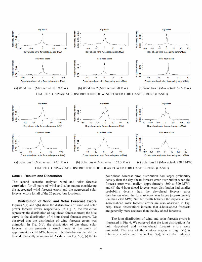
The univariate distributions of wind forecast errors are illustrated in Fig. 3. The three figures on the top show the distribution of day-ahead forecast errors; the figures on the bottom illustrate the distribution of 4-hour-ahead forecast errors. Figures 3(b) and 3(c) present the distributions of day-ahead forecast errors for wind power output in buses 2 and 8 for one principal mode and two relatively small modes; these correspond to the illustrations in Figs. 2(b) and 2(c). The distributions of day-ahead and 4-hour-ahead solar forecast errors are shown in Fig. 4. Among the 26 distributions of solar forecast errors, 22 distributions displayed a unimodal characteristic. Two typical multimodal distributions of solar forecast errors are illustrated in Figs. 4(b) and 4(c).

Pearson’s Correlation Coefficient We averaged the values of Pearson’s correlation coefficient between wind and solar forecast errors computed for the 26 pairs of wind and solar power outputs. The absolute maximum Pearson’s correlation coefficients of the day-ahead and 4-hour-ahead forecasts were estimated to be -0.08 and -0.15, respectively. In addition, the average Pearson’s correlation coefficients of day-ahead and 4-hour-ahead forecasts were estimated to be -0.03 and -0.07, respectively. Therefore, there is correlation between wind and solar power forecast errors on a single bus, though not a strong correlation. This is an important finding for power systems operations because it implies that in systems with high penetrations of both wind and solar power reserves that are held to accommodate the variability of wind or solar power can be shared.

(a) Day-ahead (pair 1) (b) Day-ahead (pair 2) (c) Day-ahead (pair 8)

(d) Four-hour-ahead (pair 1)

(Max wind actual: 110.9 MW; Max solar actual: 143.1 MW)

(e) Four-hour-ahead (pair 2) (Max wind actual: 50 MW;

Max solar actual: 340.7 MW)

(f) Four-hour-ahead (pair 8) (Max wind actual: 58.5 MW;

Max solar actual: 17 MW)

FIGURE 2. JOINT DISTRIBUTION OF WIND AND SOLAR POWER FORECAST ERRORS (CASE I)

6

(a) Wind bus 1 (Max actual: 110.9 MW) (b) Wind bus 2 (Max actual: 50 MW) (c) Wind bus 8 (Max actual: 58.5 MW)

FIGURE 3. UNIVARIATE DISTRIBUTION OF WIND POWER FORECAST ERRORS (CASE I)

(a) Solar bus 1 (Max actual: 143.1 MW) (b) Solar bus 4 (Max actual: 152.3 MW) (c) Solar bus 12 (Max actual: 228.3 MW)

FIGURE 4. UNIVARIATE DISTRIBUTION OF SOLAR POWER FORECAST ERRORS (CASE I)

Case II: Results and Discussion

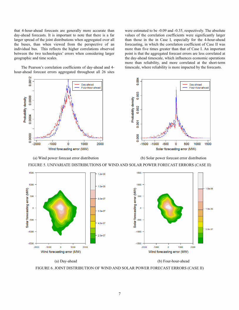
The second scenario analyzed wind and solar forecast correlation for all pairs of wind and solar output considering the aggregated wind forecast errors and the aggregated solar forecast errors for all of the 26 paired bus locations.

Distribution of Wind and Solar Forecast Errors Figures 5(a) and 5(b) show the distributions of wind and solar power forecast errors, respectively. In Fig. 5, the red curve represents the distribution of day-ahead forecast errors; the blue curve is the distribution of 4-hour-ahead forecast errors. We observed that the distribution of wind forecast errors was unimodal. In Fig. 5(b), the distribution of day-ahead solar forecast errors presents a small mode at the point of approximately -180 MW; however, the distribution can still be treated practically as unimodal. As shown in Fig. 5(a), (i) the 4-

hour-ahead forecast error distribution had larger probability density than the day-ahead forecast error distribution when the forecast error was smaller (approximately -300 to 300 MW); and (ii) the 4-hour-ahead forecast error distribution had smaller probability density than the day-ahead forecast error distribution when the forecast error was larger (approximately less than -300 MW). Similar results between the day-ahead and 4-hour-ahead solar forecast errors are also observed in Fig. 5(b). These observations indicate that 4-hour-ahead forecasts are generally more accurate than the day-ahead forecasts.

The joint distribution of wind and solar forecast errors is illustrated in Fig. 6. We observed that the joint distributions for both day-ahead and 4-hour-ahead forecast errors were unimodal. The area of the contour region in Fig. 6(b) is relatively smaller than that in Fig. 6(a), which also indicates

7

that 4-hour-ahead forecasts are generally more accurate than day-ahead forecasts. It is important to note that there is a far larger spread of the joint distributions when aggregated over all the buses, than when viewed from the perspective of an individual bus. This reflects the higher correlations observed between the two technologies’ errors when considering larger geographic and time scales.

The Pearson’s correlation coefficients of day-ahead and 4-hour-ahead forecast errors aggregated throughout all 26 sites

were estimated to be -0.09 and -0.35, respectively. The absolute values of the correlation coefficients were significantly larger than those in the in Case I, especially for the 4-hour-ahead forecasting, in which the correlation coefficient of Case II was more than five times greater than that of Case I. An important point is that the aggregated forecast errors are less correlated at the day-ahead timescale, which influences economic operations more than reliability, and more correlated at the short-term timescale, where reliability is more impacted by the forecasts.

(a) Wind power forecast error distribution (b) Solar power forecast error distribution

FIGURE 5. UNIVARIATE DISTRIBUTIONS OF WIND AND SOLAR POWER FORECAST ERRORS (CASE II)

(a) Day-ahead (b) Four-hour-ahead

FIGURE 6. JOINT DISTRIBUTION OF WIND AND SOLAR POWER FORECAST ERRORS (CASE II)

8

Case III: Results and Discussion

Case III investigated the correlation of the forecast errors arising from the aggregated power output of all 76 wind buses and 455 solar buses within the Western Interconnection of the United States.

Distribution of Wind and Solar Forecast Errors Figures 7(a) and 7(b) show the distributions of wind and solar power forecast errors, respectively. Figure 7(a) also presents a unimodal characteristic. Figure 7(b) shows the distribution of the 4-hour-ahead solar forecast errors to be multimodal. We

again observed that both the 4-hour-ahead wind and solar forecast error distributions had relatively larger probability densities than day-ahead forecast error distributions when forecast errors were smaller, and vice versa.

The joint distribution of wind and solar forecast errors is illustrated in Fig. 8. As shown, the joint distributions for both the day-ahead and 4-hour-ahead forecast errors were unimodal. The area of the contour region in Fig. 8(b) is relatively smaller than that in Fig. 8(a), which indicates that 4-hour-ahead forecasts are generally more accurate than day-ahead forecasts.

(a) Wind power forecast error distribution (b) Solar power forecast error distribution

FIGURE 7. UNIVARIATE DISTRIBUTIONS OF WIND AND SOLAR POWER FORECAST ERRORS (CASE III)

(a) Day-ahead (b) Four-hour-ahead

FIGURE 8. JOINT DISTRIBUTION OF WIND AND SOLAR POWER FORECAST ERRORS (CASE III)

9

Pearson’s Correlation Coefficient Pearson’s correlation coefficients of day-ahead and 4-hour-ahead forecasts were estimated to be -0.18 and -0.45, respectively. Table 1 lists the correlation coefficients for all three cases. It was observed that (i) wind and solar forecast errors are weakly correlated; (ii) the correlation coefficient between wind and solar forecast errors increases with the size of the analyzed region; and (iii) the absolute correlation coefficient of 4-hour-ahead forecast errors is generally greater than that of the day-ahead forecast errors.

TABLE 1 THE PEARSON'S CORRELATION COEFFICIENTS

Cases Day-ahead Four-hour-ahead

Case I -0.03 -0.07

Case II -0.09 -0.35

Case III -0.18 -0.45

CONCLUSION

This paper investigated the correlation between wind and solar power forecast errors. Both the day-ahead and 4-hour-ahead forecast errors for the Western Interconnection of the United States were analyzed. A joint distribution of wind and solar forecast errors was estimated using the KDE method.

Three cases were analyzed based on the bus numbers of the wind and solar plants. The results showed that the wind forecast error distribution was generally unimodal, and the solar forecast error distribution presented both unimodal and multimodal characteristics within different buses. The results also found that wind and solar forecast errors were weakly correlated. The absolute Pearson’s correlation coefficient between wind and solar forecast errors increased with the size of the analyzed region. As expected, 4-hour-ahead forecasts were generally more accurate than day-ahead forecasts for both wind and solar power outputs.

Future studies will quantify the impacts of the correlation between wind and solar forecast errors when assessing balancing areas’ ability to integrate wind and solar power generation.

ACKNOWLEDGMENTS

This work was supported by the U.S. Department of Energy under Contract No. DE-AC36-08-GO28308 with the National Renewable Energy Laboratory.

REFERENCES [1] Lindenberg, S., 2008, “20% Wind Energy by 2030: Increasing

Wind Energy Contribution to U.S. Electricity Supply,” Technical Report No. DOE/GO-02008-2567, U.S. Department

of Energy: Energy Efficiency & Renewable Energy, Washington, D.C.

[2] Pernick, R., and Wilder, C., 2008, “Utility Solar Assessment Study Reaching Ten Percent Solar by 2025,” Technical Report, Clean Edge, Inc. and Co-op America Foundation, Washington, D.C.

[3] Foley, A. M., Leahy, G. L., Marvuglia, A., and Mckeogh, E. J., 2012, “Current Methods and Advances in Forecasting of Wind Power Generation,” Renewable Energy, 37, pp. 1–8.

[4] Zhang, J., Chowdhury, S., Messac, A., and Castillo, L., 2012. “A hybrid measure-correlate-predict method for wind resource assessment”. In ASME 2012 6th International Conference on Energy Sustainability, San Diego, CA.

[5] Rogers, A. L., Rogers, J. W., and Manwell, J. F., 2005, “Comparison of the Performance of Four Measure-Correlate-Predict Algorithms,” J. Wind Eng. and Industrial Aerodyn., 93(3), pp. 243–264.

[6] Marquez, R., and Coimbra, C. F. M., 2011, “Forecasting of Global and Direct Solar Irradiance Using Stochastic Learning Methods, Ground Experiments and the NWS Database,” Solar Energy, 85(5), pp. 746–756.

[7] Mathiesen, P., and Kleissl, J., 2011, “Evaluation of Numerical Weather Prediction for Intra-Day Solar Forecasting in the Continental United States,” Solar Energy, 85(5), pp. 967–977.

[8] Chen, C., Duan, S., Cai, T., and Liu, B., 2011, “Online 24-h Solar Power Forecasting Based on Weather Type Classification Using Artificial Neural Network,” Solar Energy, 85(11), pp. 2856–2870.

[9] Hammer, A., Heinemann, D., Lorenz, E., and Ckehe, B. L., 1999, “Short-Term Forecasting of Solar Radiation: A Statistical Approach Using Satellite Data, Solar Energy, 67(1–3), pp. 139–150.

[10] Perez, R., Moore, K., Wilcox, S., Renné, D., and Zelenka, A., 2007, “Forecasting Solar Radiation—Preliminary Evaluation of an Approach Based Upon the National Forecast Database, Solar Energy, 81(6), pp. 809–812.

[11] Crispim, E. M., Ferreira, P. M., and Ruano, A. E., 2008, “Prediction of the Solar Radiation Evolution Using Computational Intelligence Techniques and Cloudiness Indices, Int. J. of Innovative Computing, Information and Control, 4(5), pp. 1121–1133.

[12] Chow, W. C., Urquhart, B., Lave, M., Dominquez, A., Kleissl, J., Shields, J., and Washom, B., 2011, “Intra-Hour Forecasting with a Total Sky Imager at the UC San Diego Solar Energy Testbed,” Solar Energy, 85(11), pp. 2881–2893.

[13] Marquez, R., and Coimbra, C. F. M., 2012, “Intra-Hour DNI Forecasting Based on Cloud Tracking Image Analysis,” Solar Energy, http://dx.doi.org/10.1016 /j.solener.2012.09.018.

[14] Lorenz, E., Heinemann, D., Wickramarathne, H., Beyer, H. G., and Bofinger, S., 2007, “Forecast of Ensemble Power Production by Grid-Connected PV Systems,” Proc. 20th European PV Conference, Milano, Italy.

10

[15] Methaprayoon, K., Yingvivatanapong, C., Lee, W. J., and Liao, J. R., 2007, “An Integration of ANN Wind Power Estimation Into Unit Commitment Considering the Forecasting Uncertainty, IEEE Trans. Ind. Appl., 43(6), pp. 1441–1448.

[16] Castronuovo, E., and Lopes, J., 2004, “On the Optimization of the Daily Operation of a Wind-Hydro Power Plant,” IEEE Trans. Power Syst., 19(3), pp. 1599–1606.

[17] Dietrich, K., Latorre, J., Olmos, L., Ramos, A., and Perez-Arriaga, I., 2009, “Stochastic Unit Commitment Considering Uncertain Wind Production in an isolated System,” 4th Conference on Energy Economics and Technology, Dresden, Germany.

[18] Bludszuweit, H., Domínguez-Navarro, J. A., and Llombart, A., 2008, “Statistical Analysis of Wind Power Forecast Error,” IEEE Trans. Power Syst., 23(3), pp. 983–991.

[19] Hodge, B. M., and Milligan, M., 2011, “Wind Power Forecasting Error Distributions Over Multiple Timescales,” IEEE Power and Energy Society General Meeting Proceedings, San Diego, CA, pp. 1–8.

[20] Hodge, B. M., Lew, D., Milligan, M., Holttinen, H., Sillanpaa, S., Gomez Lazaro, E., Scharff, R., Soder, L., Larsen, X. G., Giebel, G., Flynn, D., and Dobschinski, J., 2012, “Wind Power Forecasting Error Distributions: An International Comparison,” 11th Annual International Workshop on Large-Scale Integration of Wind Power into Power Systems as well as on Transmission Networks for Offshore Wind Power Plants, Lisbon, Portugal.

[21] Hodge, B. M., Hummon, M., and Orwig, K., 2011, “Solar Ramping Distributions Over Multiple Timescales and Weather Patterns,” 10th International Workshop on Large-Scale Integration of Wind Power into Power Systems as well as on Transmission Networks for Offshore Wind Power Plants, Aarhus, Denmark.

[22] Simonoff, J., 1996, Smoothing Methods in Statistics, 2 ed., Springer.

[23] Rosenblatt, M., 1956, “Remarks on Some Nonparametric Estimates of a Density Function,” The Annals of Mathematical Statistics, 27(3), pp. 832–837.

[24] Parzen, E., 1962, “On Estimation of a Probability Density Function and Mode,” The Annals of Mathematical Statistics, 33(3), pp. 1065–1076.

[25] Zhang, J., Chowdhury, S., Messac, A., and Castillo, L., 2013, “A Multivariate and Mmultimodal Wind Distribution Model,” Renewable Energy, 51, pp. 436–447.

[26] Zhang, J., Chowdhury, S., Messac, A., and Castillo, L., 2011, “Multivariate and Multimodal Wind Distribution Model Based on Kernel Density Estimation,” ASME 5th International Conference on Energy Sustainability, Washington, DC.

[27] Chowdhury, S., Zhang, J., Messac, A. and Castillo, L., 2013, “Optimizing the Arrangement and the Selection of Turbines for Wind Farms Subject to Varying Wind Conditions,” Renewable Energy, 52, pp. 273–282.

[28] Qin, Z., Li, W., and Xiong, X., 2011, “Estimating Wind Speed Probability Distribution Using Kernel Density Method,” Electric Power Syst. Research, 81(12), pp. 2139–2146.

[29] Jeon, J., and Taylor, J. W., 2012, “Using Conditional Kernel Density Estimation for Wind Power Density Forecasting,” J. American Statistical Assoc., 107(197), pp. 66–79.

[30] Juban, J., Siebert, N., and Kariniotakis, G. N., 2007, “Probabilistic Short-Term Wind Power Forecasting for the Optimal Management of Wind Generation,” Power Tech, IEEE Lausanne, pp. 683–688.

[31] Jones M., Marron J., and Sheather S., 1996, “A Brief Survey of Bandwidth Selection for Density Estimation,” J. American Statistical Assoc., 91(433), pp. 401–407.

[32] Epanechnikov V., 1969, “Non-Parametric Estimation of a Multivariate Probability Density,” Theory of Probability and Its Applications, 14. pp. 153–158.

[33] Duong T., and Hazelton M., 2003, “Plug-In Bandwidth Matrices for Bivariate Kernel Density Estimation,” Nonparametric Statistics. 15(1), pp. 17–30.

[34] Rodgers, J. L., and Nicewander, W. A., 1988, “Thirteen Ways to Look at the Correlation Coefficient,” The American Statistician, 42(1), pp. 59–66.

[35] Lew, D., 2010, “The Western Wind and Solar Integration Study,” Technical Report No. NREL/SR-550-47434, National Renewable Energy Laboratory, Golden, CO.

[36] Lew, D., 2013, “The Western Wind and Solar Integration Study Phase 2,” Technical Report No. NREL/TP-5500-55888, National Renewable Energy Laboratory, Golden, CO.

[37] Potter, C. W., Lew, D., McCaa, J., Cheng, S., Eichelberger, S., and Grimit, E., 2008, “Creating the Dataset for the Western Wind and Solar Integration Study (USA),” Wind Eng., 32(4), pp. 325–338.

[38] Hummon, M., Ibanez, E., Brinkman, G., and Lew, D., 2012, “Sub-Hour Solar Data for Power System Modeling from Static Spatial Variability Analysis,” 2nd International Workshop on Integration of Solar Power in Power Systems Proceedings, Lisbon, Portugal.