1 June 2012

Investigating the impact of offshore wind

farms on European Lobster (Homarus

gammarus) and Brown Crab (Cancer

pagurus) fisheries

Daniel J. Skerritt1, Clare Fitzsimmons1, Nicholas V.C. Polunin1, Peter Berney1,

Mike H. Hardy2,

1) School of Marine Science & Technology

Newcastle University

Newcastle upon Tyne NE1 7RU

2) Northumberland Inshore Fisheries & Conservation Authority

Unit 60B South Nelson Road

Cramlington

Northumberland

NE23 1WF

Report to

The Marine Management Organisation

June 2012

2 June 2012

Please print this report on recycled paper

Report to be cited as:

Skerritt, D.J., Fitzsimmons, C., Polunin, N.V.C., Berney, P., Hardy, M.H. (2012)

Investigating the impact of offshore wind farms on European Lobster (Homarus gammarus) and

brown Crab (Cancer pagurus) fisheries. Report to the Marine Management Organisation June 2012

3 June 2012

CONTENTS Page

SUMMARY 4

INTRODUCTION AND RATIONALE 5

1.1 Introduction 5

1.2 Rationale 6

1.3 Objectives 7

1.4 Study Area 7

METHODOLOGY 10

2.1 Fieldwork 10

2.2 Site Selection 10

2.3 Data Collection 10

2.4 Field Summary 13

MODELLING METHODOLOGY 14

3.1 Model Framework 14

3.2 Model Fitting 16

3.3 Estimating Population Size 18

3.4 Effort Modelling 18

RESULTS 19

4.1 Catch Data 19

4.2 Site Comparisons 22

4.3 Mark-Recapture Data 25

4.4 Effective Effort 26

4.5 Population size 27

4.6 Movement direction 29

DISCUSSION 31

5.1 Catch characteristics 31

5.2 Additional Outputs 33

5.3 Model Outputs 33

5.3 Model Framework and future development 34

CONCLUSION 36

ACKNOWLEDGEMENTS 36

REFERENCES 37

APPENDIX 41

4 June 2012

SUMMARY

Despite growing demand for offshore wind farms, relatively little is known about their

ecological impacts upon marine benthic fauna. Once constructed they could offer protection

from activities such as trawling and provide new artificial habitats; the degree to which

fishing is displaced and shellfish population dynamics changed is unknown. UK shellfisheries

account for over 35% of total UK landings and the evidence base for possible effects needs

urgently to be expanded. In previous Environmental Statements, methods have scarcely

informed the state of the shellfishery, but to understand future impacts, adequate baseline

data prior to construction are required. This study aims to establish four small (1km2) geo-

referenced study sites and gather baseline data for the proposed Blyth offshore

demonstration wind farm site (BODS) on movement and densities and population dynamics

of European lobster (Homarus gammarus) and brown crab (Cancer pagurus).

Differences in population structure between the areas were found. A smaller population of

lobster was present within the demonstration wind farm site than at the inshore ‘control’,

and the average size of lobster there was greater than inshore. A large population of crab,

with a larger average size was also observed at the wind farm site. However, it remains

unclear whether spatial variations in the shellfish populations are influenced by habitat

differences or other physical properties, such as distance from shore, depth of water or

temperature.

Capture and recapture rates were very low within the wind farm site, which made the

population modelling unfeasible there. The inshore site produced sufficient recaptures, and

a population of 6,163 lobsters per km2 was estimated; this figure is consistent with other

large mobile decapod density estimates. Despite poor weather impacting surveys, resulting

in insufficient data to fully exploit the proposed methodology, this study has attained

replicable and reliable catch data from within and outwith the BODS, to be used as a

baseline for future studies.

5 June 2012

INTRODUCTION AND RATIONALE

1.1 Introduction

The UK leads the world in generating electricity from offshore wind farms (OWF), with more

projects in planning or construction than any other country, and increased political and

public pressure to increase production (Smith et al., 1999). Assessments of possible OWF

locations and subsequent effects of installation must be based on existing knowledge; but,

despite growing demands, relatively little is known about their ecological impacts upon

marine benthic invertebrates and the associated fisheries. Once constructed, OWFs exclude

fishers, altering both perceptions of resource availability and subsequent fishing behaviour

(Dimech et al., 2009). Turbine arrays could provide new habitat for organisms (Landers et

al., 2001; Lacroix and Pioch, 2011; Lindeboom et al., 2011), but can also cause disturbance

to birds (Garthe and Huppop, 2004), fish (Whiteley and Taylor, 1990; Vijayakumaran et al.,

2009) and mammals (Karlsson and Christiansen, 1996; Harding and Mann, 2010); but to

what degree crustacean population dynamics change remains unknown.

Shellfish are economically important throughout Europe, yet most are managed by

comparatively few regulations; UK shellfish management measures are often locally specific,

enforced under IFCA byelaws. Stocks of several shellfish species, including European lobster

(Homarus gammarus) are considered to be fully exploited, and the UK government is

seeking improved management of key shellfish resources (Bannister, 2006; Lake and Utting,

2007). The collapse of some major finfish stocks underscores the immediate importance of

managing remaining shellfish; European Lobster form the most economically valuable part

of the catch for shellfish permit holders in the Northumberland Inshore Fisheries and

Conservation Authority (NIFCA) district (Fig. 1) (Lake and Utting, 2007), with landings of 204

tonnes in 2008, valued at an estimated £2.9 million (Aebischer et al., 1993; MFA, 2007;

Cowan, 2010; Skerritt et al., 2012). Yet knowledge gaps remain and sustainable

management of this valuable resource requires sound understanding of current fishing

activity, population dynamics, accurate and replicable baseline data, and local acceptance

and compliance with regulatory measures. Newcastle University have recently reviewed

these lobster fisheries in the NIFCA district, and have begun to quantify population

dynamics and movements via mark-recapture.

6 June 2012

Population size estimation via mark-recapture (MR) models dates back more than four

decades (Jolly, 1965; Seber, 1965). The method involves estimating probabilities of capture

(ρ) and survival/fidelity (φ), from MR data to calculate the population size implied by

observed numbers in sample catches (Dunnington et al., 2005). This approach is well-suited

to studies of fisheries resources; fishing methods by their nature capture samples of the

available population and direct observation is often impossible. MR allows for population

size estimation in an open population, with estimation of both population inputs

(recruitment & immigration) and outputs (mortality & emigration) simultaneously.

Population estimates, through MR are difficult to derive for shellfish, due to high mobility of

the animals, poorly understood behaviour, and in this instance a multi-species fishery

introducing inter-specific interactions (Cancer pagurus and H. gammarus) (Miller and

Addison, 1995; Williams et al., 2009). Despite difficulties, estimates of population via MR

have been applied to decapod crustaceans (Tremblay and Smith, 2001), for example Cancer

irroratus (Hilborn, 1997), Cancer maenas (Addison, 1997), Cancer pagurus (Bell et al., 2003),

Callinectes sapidus (Fitz and Wiegert, 1992) and Homarus americanus (Cobb et al., 1997;

Dunnington et al., 2005; Bowlby et al., 2008). Most MR approaches (Jolly-Seber and related)

are conducted over long time periods (months-years), where sampling is seen as occurring

at discrete intervals, with population dynamic processes occurring between sampling

occasions (Bell et al., 2003). However, over short time periods, the use of baited traps does

not conform to the Jolly-Seber approach, as the capture process is continuous while the trap

is set (soaking), operating alongside short-term population processes.

This study aims to build upon recent work funded by the Marine Management Organisation,

Natural England and NIFCA to develop robust MR methods (Taylor, 1982; Matsuda and

Yamakawa, 1997) and gather baseline data for European lobster, H. gammarus, prior to the

installation of turbines at the National Renewable Energy Centre’s (NaREC), BODS. This will

provide a basis from which to establish if shellfish populations are altered by OWF

installations in subsequent studies.

1.2 Rationale

Together, Newcastle University and NIFCA aim to describe small-scale European lobster

population dynamics based on a short-term continuous mark-recapture sampling method

7 June 2012

developed in previous collaborations with Natural England. The collaborative nature of the

project offers further benefits to each participating organisation, contributing to NIFCA

objectives ‘to monitor fisheries in the interest of the fishery itself and of the environment’,

while enhancing NIFCA research capacity and developing Newcastle University’s ability to

support local fisheries management.

1.3 Objectives

The objectives are:

to establish geo-referenced monitoring sites within the BODS, and appropriate

control sites outside the area

to determine shellfish distributions and population dynamics within the sites

to determine European lobster movements via tagging

to map substrate hardness within studied areas

1.4 Study Area

In August 2010 NaREC was successful in progressing a proposal for the development of the

BODS to the planning stage. Located between 1.8km and 13.8km off the east coast of

Northumberland, at Blyth, this is a 99.9MW grid-connected demonstration project with a

capacity of up to 20 large-scale prototype turbines (Fig. 1-2). Three arrays consisting of five

turbines each are currently planned, at increasing distances from shore and in depths of

approximately 35, 45 and 55 metres. Turbines will be approximately 1km apart within an

array, and arrays will be 5.5km apart.

Potting within the region is restricted by the available habitat for target species and

potential conflict with other gear types, particularly trawlers. The trap fishery targets four

main species: European lobster (H. gammarus), brown crab (C. pagurus), velvet swimming

crab (Necora puber) and prawns (Nephrops norvegicus). Many fishers use an assortment of

trap type; the majority being multi-purpose, and deployed on various ground types at

different times of year to target particular species. There are ~31 vessels under 10m in

length registered at the Port of Blyth, of which 12 are potting vessels. Each has the ability to

fish up to 800 traps within 6 nm of shore, and 95% of all Blyth potting activity occurs within

the surrounding 190km2 (Turner et al., 2009).

8 June 2012

Four survey sites were identified based on the proposed location of the BODS turbines,

previous survey sites and NIFCA knowledge; BL1 (55°08’13N, 01°22’95W); BL2 (55°06’70N,

01°23’32W); BL3 (55°04’82N, 01°21’38W) and BL4 (55°07’46N, 01°26’89W) (Fig. 2). Sites

were of differing depths, habitat and distance from turbine and shore. BL1 was located

between the two inner most arrays. Identified as an area not currently heavily fished, this

site was chosen to establish population changes between the two arrays, rather than in the

immediate vicinity, as it the case with BL2; located near to the inshore array, within an area

identified by Turner et al (2009) as an area of high potting intensity. BL3 was intended as a

control site, in similar depth but situated away from the BODS. BL4 is located inshore for

comparison between the current methods used. Six sites were initially proposed, but

weather conditions and winter daylight restricted operations. MB indicates a second site

from the 2010 winter survey, which will also be used for future analysis and comparison.

Figure 1. Northumberland coastline, the NIFCA district boundaries and major fishing ports

9 June 2012

Figure 2. Map showing the location of sampling sites, turbine arrays and ports. Overlaid on map of lobster

distribution based on landings, vessel sightings and average vessel home-range (Turner et al., 2009)

Figure 3. NIFCA Fisheries Patrol Vessel, St Oswald (ZNW04), used for the duration of this project, returning to port, North Shields

10 June 2012

METHODOLOGY

2.1 Fieldwork

All surveys were conducted on the 21m NIFCA fisheries patrol vessel, St Oswald, berthed at

Royal Quays marina, North Shields (Max/Average speed 12.7/10.8 knots) (Fig. 3). This had to

maintain its primary use as a patrol vessel, so reducing the number of days at sea. Fieldwork

commenced on the 29th October and despite two days lost to unfavourable weather was

completed on 15th December 2011.

2.2 Site Selection

Four survey sites were selected within the NaREC indicative layout, using local NIFCA

knowledge to minimise interaction with other fishing gear. One was selected near a random

turbine in array 2 (BL2), one within the BODS site (BL1) and one as a control (BL3). The final

site (BL4) was introduced to ensure the rigour of the methodology by repeating a site that

had been successfully sampled and modelled the previous winter. BL1 was dominated by

‘soft’ sediment, with slightly ‘harder’ areas in the north and west of the site (Fig. 14.a);

average depth of the site was 41.3m (min 38.8m; max 44.1m). BL2 was also dominated by

‘soft’ sediment, but was less homogeneous than BL1, with ‘harder’ areas to the north-west,

and central-southern areas of the site with an average depth 35.2m (min 29.7m; max

39.8m) (Fig. 14b). Habitat at BL3 and BL4 was much ‘harder’, with extensive areas of rock and

cobble (Fig 14c & 14d, respectively); average depth was 38.9m at BL3 (min 34.2m; max

42.8m), and 27.2m at the inshore BL4 site, which also had much more variance in depth, so

forming a more complex habitat (min 16.7m; max 31.8m). The substrate distribution and

depths in the areas outside of the immediate study areas have been interpolated from

known substrate hardness at the sites.

2.3 Data Collection

Standard steel framed parlour traps 0.66m in length were used, with 27mm mesh and

selective grill on the bottom and 130mm fixed diameter, single-side entrance. Traps were

arranged in eight identical fleets of eight traps (A-H; West-East), running North to South at

11 June 2012

each site (1-8; North-South), spaced approximately 40m between traps and 100m between

fleets. Traps were baited with one frozen flatfish per trap (Fig. 4).

On setting the fleets, the vessel was lined up to predetermined fleet positions using the on-

board navigation software, with a due North bearing. Fleets were then set once the vessel

was at the correct position and released at a speed of 3.5 knots.

Figure 4. Images of the indicative trap layout at BL4 (top); one fleet of eight traps prior to being set (bottom-left),

and image of the standard parlour trap, a: length of trap (0.66m), b: width (0.46m), and c: mesh size (27mm),

baited with flatfish (bottom-right)

a

b c

Blyth

¯0 0.5 10.25 Kilometers

Legend

BL4

3_mile_limit_OSGB

12 June 2012

The study consisted of hauling all 64 traps (8 fleets of 8 traps) at three day intervals over a

two week period, so all fleets were hauled four to five times at each site (Average soak time:

3.7 days; Min: 2 days; Max: 6 days) (Fig. 5). Fleets were allowed to soak for four to five days

prior to the first sampling occasion, to generate a sample of animals for marking. Position of

fleet and water depth were recorded for each trip, as fleets and traps can move during

unfavourable weather, shooting and resetting of the fleet, and from interaction with other

sea users. In fleets of traps, catch rates are often highest in the traps at the ends of the

fleets. One possible interpretation of this observation is that the individual trapping areas

interfere with one another (Fig. 7), therefore the distance between traps in this study was

increased from 20m standard commercial distance to 40m.

On hauling, all lobster caught were tagged with a persistent T-bar tag (Hallprint Pty Ltd,

Aus.), inserted just behind the carapace, into the abdominal musculature, offset to avoid the

alimentary canal and vital organs (Fig. 6). Inserted correctly they should remain post-

ecdysis, resulting in an individual lobster being identifiable for several seasons. Each tag has

an individual ID number printed on it making it possible to construct accurate capture and

movement records for each marked lobster (Fig. 6). All captures were released, unless

seriously damaged, in which case they were recorded as removed from the experiment.

Figure 5. The date of setting and hauling of fleets at all sites during the 12 week study period

13 June 2012

Release location was at the approximate location of the trap from which they were

captured. Additionally biometric data was recorded for every individual lobster and crab;

including carapace length/width (CL/CW) respectively (rear of eye socket to base of the

carapace for lobster), sex, species, and presence of eggs, general condition, and their

capture location (site, fleet and trap number).

2.4 Field Summary

The project ran smoothly, in part due to the strength of the working relationship between

Newcastle University, NIFCA, and the local fishing community. The initial start date was

planned for summer, with two sites conducted in July, two in August and two in September,

but delays to the project start date resulted in a winter survey, which had some adverse

implications. Traps were lost on only one occasion; the fleet was re-shot with replacement

traps, minimising impact, and the data removed from future analysis. The main issue was

the cutting of the lines to fleets on sixteen occasions, probably due to sites being located

near busy shipping lanes, which added time constraints. The study consisted of 20 sampling

days split between four sites (Fig. 5). Previous catch data demonstrates that lobster

numbers are lower during winter months, consequently low recaptures will weaken the

modelling methodology and subsequent population estimates. In total 206 European

lobsters were tagged with persistent individual T-bar tags, this will enable the continued

monitoring of their movements via commercial recapture. With such low numbers at BL1,

Figure 6. Images showing lobster with T-bar tag inserted into the abdominal musculature (top left), the tagging gun

and tags (top right), and the printed tags (bottom left)

14 June 2012

BL2 and BL3 analysis of the population at each site will be difficult, but total population

numbers are high enough for strong analysis of the population demographic as a whole. A

successive study period for the summer of 2012 is planned, to make up for the shortfall in

sampling occasions.

MODELLING METHODOLOGY

3.1 Model Framework

A general model framework for MR data was defined (Bell et al., 2003), in which a cohort of

marked lobster was released. Subsequent sampling was used to recapture the survivors

(those that remain in the study area), which were then re-released at approximately the

same place (and time) of capture. Consequently, a marked individual could be captured

several times, generating a capture history (CH) (Burnham et al., 1987); the probability of a

particular CH occurring can be predicted by parameters describing capture, movement, and

survival processes between release occasions. However, Jolly-Seber methods consider the

capture process as discrete; whereas short-term trap fishing is a continuous process

(capture could occur at any point between setting and hauling). Therefore population

processes are described over shorter intervals than the time between sampling occasions

(Dunnington et al., 2005). This can be either tidal or diel intervals, depending on the

sampling intervals. Tidal is a behaviourally meaningful period (Smith et al., 1999) that also

allows for easier specification of models for unequal sampling intervals; however, as all

fleets were hauled on the same day during this study, a diel is considered sufficient.

As with all MR methods, key assumptions made were: (1) tagged individuals mix freely with

the untagged population; (2) tags remain present or the rate of tag-loss is known; (3)

capture and tagging does not alter survival or behaviour that would change capture

probability relative to untagged or non-captured individuals; (4) individuals that leave the

study area do not return to the study area (Lebreton et al., 1992); and (5) species

interactions do not affect capture rate (See 4.8).

For each tagged individual one of three observed states was recorded for each tide after

first release, to generate the CH: 0 not observed; 1 captured and released; -1 captured and

15 June 2012

removed. The 0 state was recorded if no traps were hauled that day or if the tagged lobster

was not observed on a haul occasion.

The overall probability of a particular CH occurring is the product of a series of probabilities

of the possible fate of the individual over each day following marking and first release. Given

its availability in the ‘capture area’ (area over which experimental traps exercise an influence

and the area in between and around traps from which a lobster could potentially return to

the area of influence during the study (Bell et al., 2003) (Fig. 20), three possible fates could

be defined: (1) the lobster does not enter a trap, but remains in the capture area; (2) the

lobster enters a trap and is observed; (3) the lobster does not enter a trap and permanently

emigrates from the capture area.

The respective probabilities of each fate can be described by the following three equations:

The probability that a lobster is present in the capture area but not caught between times t1

and t2 can be calculated as:

[Eq. 1]

Where ρi is probability of capture per unit of effort over tide i; φi the fidelity to the capture

area over tide i; and fij the fishing effort exerted by fleet j over tide i. ‘Fidelity to capture

area’ is defined here as remaining available for capture: not emigrating, dying or losing the

tag.

The probability a lobster enters a trap in fleet j between times t1 and t2 can be calculated as:

[Eq. 2]

Equation [1], refers to the probability of not being captured in any fleet, so the effort is

summed across all fleets , whereas equation [2] demonstrates the probability of being

captured in one particular string, j; .

The probability of a lobster permanently leaving the capture area between times t1 and t2

can be calculated as;

[Eq. 3]

2

11 1

2

11

t

ti

i

J

j

iji

t

tfpU

2

11

1

1

2

1)(

t

ti

iji

i

t

t

tfpUjV

2

11 1

1

1

2

111

t

ti

i

J

j

iji

i

t

t

tfpUW

J

j

ijf1

ijf

16 June 2012

Given values of ρi, φi and fij, the probability of any CH can be calculated, from a combination

of equations [1-3].

Each CH probability takes into account the history of setting and hauling of each fleet during

the experiment, which allows for difficulties encountered from incomplete sampling of the

sites, especially during winter conditions. The approach taken assumed that average capture

probabilities in the fleets hauled on any given occasion were consistent with average

capture probabilities across all fleets (i.e. ρij = ρi for all j).

Given pre-determined values of fishing effort, f, (see section 2.6) for each hauling occasion i

and fleet of traps j, the model framework can be used to obtain estimates of ρi and φi from

MR data. Initial values of ρ and φ were constrained to 1, as no trap effects would be

observed in the first instance. Ultimately, it is the ρ and φ values that are the fundamental

quantities from which the CH probabilities are constructed (Lebreton et al., 1992).

3.2 Model Fitting

The probabilities of each observed CH were combined with the CH frequencies to calculate

the likelihood function (likelihood of a set of parameter values given observed outcomes are

equal to the probability of those observed outcomes given those parameter values). The

goal of the model fitting was to maximize this likelihood by adjusting the survival and

recapture probabilities. Twenty-five possible models were defined for the MR data, from

the most complex model (ρsex*time, φsex*time), to the simplest possible model with parameters

constant across time and between sexes (ρ, φ). The most parsimonious model and robust

basis for inference about population size was selected by minimum value of the Akaike

Information Criterion (AIC), in its bias-adjusted form, AICc (Burnham et al., 1987), calculated

as;

[Eq. 4]

[Eq. 5]

kLLAIC 2ln2

12ln2

kn

nLLAIC

C

17 June 2012

Where lnL is the log-likelihood for the model, k is the number of separately identifiable

model parameters and n is the sample size (number of marked individuals) (Burnham &

Anderson 2002).

MR data were presented in reduced m-array format (Table 1), observed and expected m-

array totals with χ2 contributions for a goodness-of-fit (GoF) test for all suitable models to

find the most parsimonious. Because low numbers of captures and few recaptures might

have yielded low power for the GoF tests, pooling by column (grey cells) was used. Total

numbers released on each occasion included recaptured, previously marked lobster added

to the newly marked lobster caught for the first time. Expected values were generated by

multiplying the model output probability of a particular capture history by the number of

new released individuals. Degrees of freedom were calculated as number of cells that

contribute to the χ2 value, minus number of model parameters (i.e. 11 – 2 = 9), the

contribution of each pooled cell to the GoF test statistic is shown in table 1. The P value at

the bottom shows a particularly good fit of the model with the data, therefore we accept

that the model is suitable to continue with population estimates.

Table 1. Reduced m-array (Burnham et al., 1987) showing observed, expected and χ2 values for the model (ρ, φ) at the BL4 site, used for GoF testing. Each row represents first recapture for a given release cohort.

Recaptures are added to the release totals, so that multiple recaptures are pooled with first recaptures from a new release cohort.

18 June 2012

3.3 Estimating Population Size

ρ and φ allow for appropriate scaling of catch data to obtain estimates of the size of the

local population from which the catches were drawn. These catch by fleet data were used to

obtain a separate estimate of population size from each fleet on each haul, thus, treating

each fleet catch as a realisation of average fleet catches over the whole capture area; this

avoided problems of definition of capture areas for individual fleets.

To calculate the population N, of a given fleet j, over a given tide t, we used the following

formula:

[Eq. 6]

Equation 6 was used to give separate population estimates from each observation of the

catch by a fleet, thus, treating each fleet’s catch as an average of all fleet catches over the

whole capture area.

Bootstrapping was not conducted on these data in the current report, instead variation

between individual fleet hauls was considered, and produced much larger confidence

intervals (Bell et al., 2003). Because spatial heterogeneity would inflate the variance of the

overall population estimate combined over all catches, the median of all estimates was

taken to reduce the impact of outliers.

3.4 Effort Modelling

Given unequal soak times and capture probabilities defined at the temporal scale of

individual tides, it was essential to adjust the effective fishing effort applied by each fleet on

each tide of its soak. Catches are commonly assumed to have asymptotic relationships with

soak time, due to trap saturation and declines in attractiveness of bait (Briand et al., 2001):

[Eq. 6]

Where C∞ is the asymptotic catch (maximum possible catch), Ct the catch for soak time of t

and b the rate at which the increase in catch declines over time.

If the effective effort exerted by a fleet of traps j is set equal to 1 over the first tide of soak

time, the effective effort on any subsequent tide is given as:

fffp

CN

jij

tj

tj**

bteCCt

1

19 June 2012

[Eq. 7]

No independent estimates of b exist for European Lobster, so the catch data from this

experiment were used to infer a value. The approach to assume a value of C∞ and estimate

b from the relationship by simple linear regression without an intercept, for effective effort

is unlikely to introduce serious biases into the population estimates.

The approach was:

[Eq. 8]

RESULTS

4.1 Catch Data

To test for interactions between fleets and traps the difference in catch rates of total

animals was tested between outside fleets (A and H) and inside fleets (B to G), and between

end traps (1 and 8) and inside traps (3 to 6). Average total catch rates did not differ

significantly between outside and inside fleets at BL2 (t-test: Total12 = P=0.559), BL3 (t-test:

Total18 = P=0.115) or BL4 (t-test: Total13 = P=0.733), but did significantly differ at BL1 (t-test:

Total24 = P=0.028). However, to minimise effects of unusually high catches that occurred on

inside fleets at BL1, the average catch of each fleet over the whole study period was used to

test for differences between outside and inside fleets at BL1; like the other sites, there was

no significant difference (t-test: Total6 = P=0.092). No significant difference between the

average catch of end traps and middle traps was observed at any site (BL1, BL2, BL3 and BL4

t-test: Total46 = P=0.246, 0.208, 0.162, and 0.343 respectively).

b

jiijeff

,1

t

tjb

C

CLn

1

Figure 7. Trap interaction visualisations (Bell et al., 2001); a. circles represent overlap of trapping areas, of radius

r, for three baited traps; b. overlap relating to capture probability, Pcapture, to distance from trap.

20 June 2012

In total 200 individual lobsters were caught (BL1 10; BL2 43; BL3 12; BL4 135) in 19 hauls at

the four sites; 91 were male and 115 were female, (M:F =1:1.26). The size distributions of

male and female lobsters were normally distributed around ~80mm (Fig. 8a). There was a

decrease in observations at 85-95mm, when the lobsters reach legal landing size (MLS =

87mm), 74% of the lobster caught being below MLS (Fig. 9). A second size peak ~93mm was

observed, that was not as obvious in 2010. There was no significant difference in mean CL

between male and female lobsters (t-test; Sex198, P=0.70). Fewer undersized lobsters were

observed in 2011 than 2010 (Fig. 8b), but no significant difference in the size distribution of

lobster between 2010 and 2011 (t-test: Year552 P<0.05). The distributions between 80 and

90mm were precisely matched between the years. Approximately 15% of the observed

female population had eggs present (ovigerous). The average CL of ovigerous females was

89.6 mm, however 41% of the ovigerous females were under the MLS of 87mm, with the

smallest size recorded at 79mm.

0

5

10

15

20

25

30

45

50

55

60

65

70

75

80

85

90

95

10

0

10

5

11

0

11

5

Mo

re

CL (mm)

a. Male and female lobster size distribution 2011

Male = 91

Female = 115

0

2

4

6

8

10

12

14

16

35

40

45

50

55

60

65

70

75

80

85

90

95

10

0

10

5

11

0

11

5

12

0

12

5

CL (mm)

b. Population size distribution of lobster 2010/2011

3 per. Mov. Avg. (2010)

3 per. Mov. Avg. (2011)

Figure 8. a. Size distribution of all female and male lobster caught throughout the survey period, 2011. b. Size distribution of all

lobster caught during the 2011 study (Red) against the size distribution of all lobster caught in the 2010 survey, MLS of 87mm

is represented by orange vertical line.

MF

120

110

100

90

80

70

60

CL (

mm

)

Lobster Sex Distribution

Figure 9. Distribution of CL between the sexes of lobster.

21 June 2012

In total 5,736 individual brown crabs were caught throughout the duration of the study (BL1

3,596; BL2 872; BL3 461; BL4 807) in 19 hauls at the four sites; 3,950 were male and 1,786

were female (Fig. 11a; F:M =1:2.22). There is a significant difference between the CW of

male crabs and females crab (t-test, Sex2811, P<0.05), with the male mean being slightly

lower than the female; however, female distribution was slightly skewed towards the

smaller size range (Fig. 10 and 11a). There was no obvious decrease in observations as the

crab become legal to land (MLS>130mm). In 2010, most crab observed were well below the

MLS, in part due to large numbers of juvenile crab observed at a homogeneous sandy

inshore site. When the offshore sites are excluded from the 2011 population (Fig. 11b, green

line), the graph more closely resembles that of 2010 (Fig. 11b).

0 50

100 150 200 250 300 350 400 450

65

75

85

95

10

5

11

5

12

5

13

5

14

5

15

5

16

5

17

5

18

5

19

5

20

5

Mo

re

CW (mm)

a. Female and male total Crab population

Female = 1,786

Male = 3,950

0

5

10

15

20

25

30

35

0

20

40

60

80

100

120

140

160

54

63

72

81

90

99

10

8

11

7

12

6

13

5

14

4

15

3

16

2

17

1

18

0

18

9

19

8

20

7

21

6

CW (mm)

b. Population size distribution of lobster 2010/2011

3 per. Mov. Avg. (2010)

3 per. Mov. Avg. (2011)

3 per. Mov. Avg. (2011 BL4 ONLY)

Figure 11. a. Size distribution of all female and male brown crab caught throughout the survey period, 2011. b. Size distribution of

all brown crab caught during the 2011 study (Red) against the size distribution of all in the 2010 survey, and 2011 inshore site BL4

only. MLS of 130mm is represented by orange vertical line.

MF

225

200

175

150

125

100

75

50

CW

(m

m)

Crab Sex Distribution

Figure 10. Distribution of CW between the sexes of crab.

22 June 2012

4.2 Site Comparison

Significantly more lobster were caught at the inshore site BL4 (catch per unit effort (CPUE) =

7.95 ±0.51) (Fig. 13 g) in the same period as at the three offshore sites: BL3 (CPUE = 0.91

±0.02); BL2 (CPUE = 2.95 ±0.12); BL1 (CPUE = 0.86 ±0.03) (Fig. 13 a, c, e). Mean CL of lobster

differed among sites (one-way ANOVA3; P<0.05); BL1, BL2, and BL3 were not significantly

different from each other (Fisher, post-hoc) but BL4 had lower mean CL than both BL2 and

BL3 (Fisher post-hoc; -6.52, 95% confidence range for mean difference (CR)) (Fig. 12b).

Highest observed crab catches, however, were offshore: BL1 (CPUE = 309.71 ±12.17), BL2

(CPUE = 59.75 ±2.49), and BL3 (CPUE = 34.85 ±0.95) (Fig. 13b, d & f). Inshore site BL4 crabs

were negatively skewed towards the smaller sizes (Fig. 13h), rather than normally

distributed as at BL1 and BL2 (CPUE = 46.52 ±2.99).

Mean CW of crabs also differed among sites (one-way ANOVA3; P<0.05). BL4 had a

significantly lower mean CW than the other sites (Fisher’s post-hoc, -19.31 95% CR), and BL3

was slightly lower than BL2; however BL1, BL2, and BL3 had similar mean CW (Fisher post-

hoc,-4.30 95% CR) (Fig. 12a). BL1 and BL2 had the largest crab population size and CW values

(Fig. 13b, d & Fig. 14a, b). BL1 (Fig. 14a) and BL2 (Fig. 14b) were similar in substrate and

depth although BL2 had more areas of hardness, distributed to the south of the study area.

BL3 (Fig. 14c) and BL4 (Fig. 14d) had much larger proportions of rock and cobble.

BL4BL3BL2BL1

225

200

175

150

125

100

75

50

CW

(m

m)

a. Crab Size Distribution

BL4BL3BL2BL1

120

110

100

90

80

70

60

CL (

mm

)

b. Lobster Size Distribution

Figure 12. a) Size distribution of crab caught at each site. b) Size distribution of lobster caught at each site

23 June 2012

0

5

10

15

20

25

30

35

45

50

55

60

65

70

75

80

85

90

95

10

0

10

5

11

0

11

5

Mo

re

Fre

qu

en

cy

CL (mm)

c. BL2 lobster population

n = 44

0

5

10

15

20

25

30

35

45

50

55

60

65

70

75

80

85

90

95

10

0

10

5

11

0

11

5

Mo

re

Fre

qu

en

cy

CL (mm)

g. BL4 lobster population

n = 135

0

20

40

60

80

100

120

140

65

75

85

95

10

5

11

5

12

5

13

5

14

5

15

5

16

5

17

5

18

5

19

5

20

5

Mo

re

Fre

qu

en

cy

CW (mm)

f. BL3 crab population

n = 947

0

20

40

60

80

100

120

140

65

75

85

95

10

5

11

5

12

5

13

5

14

5

15

5

16

5

17

5

18

5

19

5

20

5

Mo

re

Fre

qu

en

cy

CW (mm)

d. BL2 crab population

n = 1,218

0

20

40

60

80

100

120

140

65

75

85

95

10

5

11

5

12

5

13

5

14

5

15

5

16

5

17

5

18

5

19

5

20

5

Mo

re

Fre

qu

en

cy

CW (mm)

h. BL4 crab population

n = 1,048

0

5

10

15

20

25

30

35

45

50

55

60

65

70

75

80

85

90

95

10

0

10

5

11

0

11

5

Mo

re

Fre

qu

en

cy

CL (mm)

e. BL3 lobster population

n = 12

Figure 13 a-h. Observed population size-frequency distribution of European lobster (a, c, e, g) and brown crab (b, d, f, h)

0

50

100

150

200

250

300

65

75

85

95

10

5

11

5

12

5

13

5

14

5

15

5

16

5

17

5

18

5

19

5

20

5

Mo

re

Fre

qu

en

cy

CW (mm)

b. BL1 crab population

n = 2,450

0

5

10

15

20

25

30

35 4

5

50

55

60

65

70

75

80

85

90

95

10

0

10

5

11

0

11

5

Mo

re

Fre

qu

en

cy

CL (mm)

a. BL1 lobster population

n = 10

24 June 2012

Figure 14 a-d. Screenshots of Olex data for BL1 (a), BL2 (b), BL3 (c), and BL4 (d). The substrate hardness is mapped via a colour scale

from purple (0% hardness) through blue, yellow to red (100% hardness). Inset (upper) depth transect of fleet A (westerly fleet) from

each site.

a.

.

b.

c. d.

Figure 15. Lobster population size estimates for individual fleets from model φ (), ρ (), at BL4, showing mean estimates (circles), median,

and interquartile range (box).

HGFEDCBA

12000

10000

8000

6000

4000

2000

0

Fleet

Popula

tion S

ize

25 June 2012

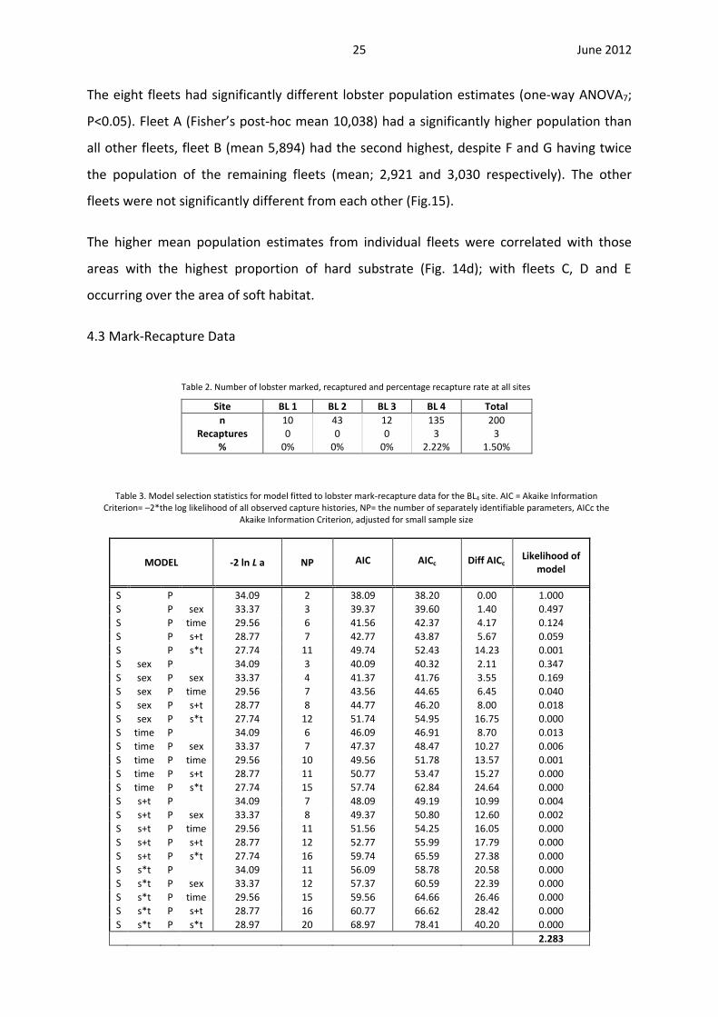
The eight fleets had significantly different lobster population estimates (one-way ANOVA7;

P<0.05). Fleet A (Fisher’s post-hoc mean 10,038) had a significantly higher population than

all other fleets, fleet B (mean 5,894) had the second highest, despite F and G having twice

the population of the remaining fleets (mean; 2,921 and 3,030 respectively). The other

fleets were not significantly different from each other (Fig.15).

The higher mean population estimates from individual fleets were correlated with those

areas with the highest proportion of hard substrate (Fig. 14d); with fleets C, D and E

occurring over the area of soft habitat.

4.3 Mark-Recapture Data

Table 2. Number of lobster marked, recaptured and percentage recapture rate at all sites

MODEL -2 ln L a NP AIC AICc Diff AICc Likelihood of

model

S

P 34.09 2 38.09 38.20 0.00 1.000

S

P sex 33.37 3 39.37 39.60 1.40 0.497

S

P time 29.56 6 41.56 42.37 4.17 0.124

S

P s+t 28.77 7 42.77 43.87 5.67 0.059

S

P s*t 27.74 11 49.74 52.43 14.23 0.001

S sex P 34.09 3 40.09 40.32 2.11 0.347

S sex P sex 33.37 4 41.37 41.76 3.55 0.169

S sex P time 29.56 7 43.56 44.65 6.45 0.040

S sex P s+t 28.77 8 44.77 46.20 8.00 0.018

S sex P s*t 27.74 12 51.74 54.95 16.75 0.000

S time P 34.09 6 46.09 46.91 8.70 0.013

S time P sex 33.37 7 47.37 48.47 10.27 0.006

S time P time 29.56 10 49.56 51.78 13.57 0.001

S time P s+t 28.77 11 50.77 53.47 15.27 0.000

S time P s*t 27.74 15 57.74 62.84 24.64 0.000

S s+t P 34.09 7 48.09 49.19 10.99 0.004

S s+t P sex 33.37 8 49.37 50.80 12.60 0.002

S s+t P time 29.56 11 51.56 54.25 16.05 0.000

S s+t P s+t 28.77 12 52.77 55.99 17.79 0.000

S s+t P s*t 27.74 16 59.74 65.59 27.38 0.000

S s*t P 34.09 11 56.09 58.78 20.58 0.000

S s*t P sex 33.37 12 57.37 60.59 22.39 0.000

S s*t P time 29.56 15 59.56 64.66 26.46 0.000

S s*t P s+t 28.77 16 60.77 66.62 28.42 0.000

S s*t P s*t 28.97 20 68.97 78.41 40.20 0.000

2.283

Table 3. Model selection statistics for model fitted to lobster mark-recapture data for the BL4 site. AIC = Akaike Information Criterion= –2*the log likelihood of all observed capture histories, NP= the number of separately identifiable parameters, AICc the

Akaike Information Criterion, adjusted for small sample size

Site BL 1 BL 2 BL 3 BL 4 Total

n 10 43 12 135 200 Recaptures 0 0 0 3 3

% 0% 0% 0% 2.22% 1.50%

26 June 2012

Recapture rates were exceptionally low; of the 200 individual lobster marked, only three

(1.5%) were recaptured. No recaptures occurred at the offshore sites; BL4 had a recapture

rate of 2.2% (Table 2). Due to the lack of recaptures, movement and fidelity to the capture

area cannot be estimated for sites BL1, BL2, and BL3.

Catch data from BL4 were used to estimate fidelity (φ) and capture (ρ). The minimum AICc

value, indicating the most parsimonious model of fidelity and capture probabilities for the

data, was for the simplest of models φ (), ρ () (Table 3). The model indicated probability of

capture and fidelity to the capture area was influenced neither by sex or time.

The probability of capture was low (ρ = 0.0036), did not change over time or between sexes.

Fidelity to the capture area also remained constant over time and between sexes, and was

very high (φ = 0.9999908).

With some reservations about heterogeneity of capture probabilities and fidelity, the model

φ (), ρ () sufficiently fits the data (GoF, BL49, χ2 = 4.73, d.f. = 9, P>0.05), and is an adequate

basis for inference about population size at BL4.

4.4 Effective Effort

As there is a lack of variation in soak time, no clear signal about the effect of soak time on

catch rates could be derived. The estimates of b show relatively narrow ranges of variation

(Fig. 16 a-d), but inferences from this relationship can only be weak. There was insufficient

information to quantify the maximum possible catch C∞, although catch data per day

declined with increased soak time and can be used to estimate C∞. The effort adjustment

was found to be relatively insensitive to choice of C∞ over a range of possible values (Bell et

al., 2003), so a value of 216 was used (C∞= highest observed n in trap+1 * number of traps

((26 +1) * 8 traps = 216)). The rate of increase in effective effort over time was calculated for

each site.

27 June 2012

4.5 Population size

Although recaptures were low at BL4, the GoF test suggests the chosen model is a good fit

for the data. From Eq. 6, using probabilities of ρ from model φ (), ρ (), and assuming that ρ

remains constant temporally, the catch data at BL4 suggest a population of about 1,730

lobsters within the 0.28 km2 capture area of the study (Fig. 17), a density of 6,163

lobsters/km2.

The large variation in the population estimate (Fig. 17) is attributable to the high catch rates

of fleets A and B (one-way ANOVA; P<0.05; Fig. 15). The wide confidence limits reflect the

high spatial variation (Fig. 18), but population estimates did not vary among occasions (one-

way ANOVA; P>0.05). CPUE show a similar pattern over time to that of population estimates

(Fig. 19), indicating that estimates may be driven largely by differences of catch rather than

ρ and φ.

The model output gives an estimate of lobster density in the 0.28 km2 area surrounding the

experimental fleets of traps (Fig. 20). Although this population is not closed, average

turnover (= 1- φ) was exceptionally low, <1% of the population emigrating during each study

day, with no difference observed between males and females. Most recaptures were also

0

2

4

6

8

10

0 5 10 15 20

Effe

ctiv

e Ef

fort

Soak Time

BL4 - b

0

2

4

6

8

10

0 5 10 15 20

Effe

ctiv

e Ef

fort

Soak Time

BL1 - b

0

2

4

6

8

10

0 5 10 15 20

Effe

ctiv

e Ef

fort

Soak Time

BL2 - b

0

2

4

6

8

10

0 5 10 15 20

Effe

ctiv

e Ef

fort

Soak Time

BL3 - b

Figure 16. Relationships between effective effort and soak time from catch data at each site, calculated from point estimate and 95% CI for b.

28 June 2012

within close proximity of their first capture site (<2km), with very few individuals migrating

greater distances.

The capture area, over which this population estimate applies, must then be calculated, to

determine the density. As boundaries of the study site are theoretical, and little information

exists on movements of European lobster, it was assumed that the population of lobster

was drawn from the area between and surrounding the traps; a minimum convex polygon

50m in diameter being assumed (Fig. 20). The minimum estimate was generated by taking

the only reported home-range estimation of H. gammarus, (Moland et al., 2011), and the

area of bait influence (Bell et al., 2001). It is unlikely the catch is drawn from a much greater

area than this, given the low population turnover and as no overlap was observed between

catches of fleets or traps (Section 4.1).

14131211109876543210

12000

10000

8000

6000

4000

2000

0

Haul Occassion

Popula

tion S

ize

6000

5000

4000

3000

2000

1000

Po

pu

lati

on

Siz

e

Figure 17. Lobster population estimates, with 95% CI quartiles displayed by the box

Figure 18. Lobster population size estimates for individual capture occasion.

29 June 2012

4.6 Movement direction

General movement vectors were inferred via tagging of individual lobsters and mapping the

vector formed between site of first capture and subsequent recapture locations, either

within the study area, or via commercial recapture. The mean linear directional movement

of all recaptures was 62o which is approximately North-East-East, but has a large variation

(0.76) and the mean movement distance was 510m. Mean directional movements for

female lobster were 91o, due East, again with large variation, and a mean length of 354m.

Male lobster mean directional movement was 41o, North East, with similar variation (0.73),

and mean distance of 633m (Fig. 21). No significant difference between distance moved

between sexes was observed (t-test: P= 0.437). Individuals recaptured during study periods

¯0 0.5 10.25 Kilometers

Legend

Pots

Capture_Area

Figure 20. Illustration of the capture area 299975 m2, formed from a minimum convex polygon of diameter 55m.

1

1.2

1.4

1.6

1.8

2

2.2

2000

2500

3000

3500

4000

4500

5000

0 5 10 15

Ave

rage

CP

UE

Po

pu

lati

on

Siz

e

Soak time

Population Size

CPUE

Figure 19. Average lobster population size for each capture occasion (square) and CPUE (diamonds)

30 June 2012

in 2010 and 2011 and from subsequent commercial sector recapture show predominantly

south-east movements from their initial release location.

DISCUSSION

5.1 Model outputs

Compared with other studies of decapod species (Eggleston et al., 1999; Dunnington et al.,

2005; Bowlby et al., 2008; Agnalt et al., 2009) our estimate of 6,163 lobsters per km2 at BL4,

is relatively low. A MR approach showed the un-fished northern fjords of Norway to hold a

population of 15,576 H. gammarus per km of shoreline (Agnalt et al., 2009). Population

estimates for H. americanus were generally higher, Rowe (2002) finding on average 10,000-

20,000 per km2, falling as low as 2,500 per km2 depending on substrate type

(Newfoundland, Canada). In contrast Dunnington et al. (2005) found 65,000 per km2 at their

summer peak via MR (Maine, US), however Bowlby (2008) found as few as 400-450 per km2

(Northumberland Strait, Canada). Previous studies conducted by Newcastle University using

similar methods to this study revealed densities of 2,359 per km2 and 9,096 per km2 for H.

gammarus at a study site ~750m South-west of BL4 and at MB (Fig.2) respectively (Skerritt et

al., 2011; Skerritt et al., 2012).

H. gammarus is perhaps more suited to MR methodologies than H. americanus, as the latter

are thought to disperse further (Smith et al., 1998; Frusher and Hoenig, 2003), increasing

turnover rate at a site and perhaps also the likelihood of overestimating populations. The

fidelity estimate (p) of 0.99 shows little or no turnover of population at the timescale

involved and one order of magnitude lower than previous years, probably due to the low

number of recaptures. Movement rates were lower than 2010 data where fidelity was 0.97

and 0.93 for Blyth and MB respectively. This would be expected during the winter months,

when activity levels of lobster are at their lowest (Smith et al., 1999; Moland et al., 2011).

Despite uncertainties, the data derived here and previously are winter estimates that are

considered to be on the low side (Skerritt et al., 2012). However, taking into account the

generally higher recorded catch rates of H. americanus, these estimates given here appear

to be reasonable, and are the first estimates of this kind for UK H. gammarus.

31 June 2012

5.2 Catch characteristics

The size distribution of total lobster was skewed towards smaller sizes (<MLS), due to

mortality and removal of larger individuals by fishing (Fig. 8a). There were fewer large male

lobster than females (Fig. 8a & 9, Q3=89mm) (Lizarraga-Cubedo et al., 2003), male C.

pagurus were also significantly smaller than females (Karlsson and Christiansen, 1996; Woll

et al., 2006; Harding and Mann, 2010). Male crab catch rates were over twice as high as

those of females throughout the study period; unlike lobster, berried crabs are rarely seen

in traps, which could account for some reduction in observations (Howard, 1982; Woll,

2003). A repeat study in the summer months would highlight any seasonal variation in sex

proportion of C. pagurus or H. gammarus. Reduced observations of undersized lobsters in

2011 compared with 2010, and a second peak around ~93mm (Fig. 7b) is attributed to a

spatial influence between inshore and offshore sites. Catch is lowest for lobster further

offshore with greater average depths. For crab, the offshore sites had higher catch rates

than inshore.

Lobsters were smaller at BL4 possibly due to interactions with high catch of crabs at offshore

sites, but more likely a difference in habitat type (Fig. 13d), (Tremblay and Smith, 2001) as

juvenile lobsters rely more heavily on habitat cover for predation avoidance than adults

(Herrnkind et al., 1997; Selgrath et al., 2007; Hovel and Wahle, 2010). The predominance of

hard habitat inshore could explain the slightly lower mean crab CW at BL3 (Figs. 13) and BL4

(Fig. 11a). Offshore sites in and around the BODS support a much larger average size of C.

pagurus and H. gammarus than inshore sites; this could be due to a natural size-led spatial

distribution, increased fishing pressure at inshore sites resulting in the removal of animals

>MLS, or the influence of habitat type.

Refuges are important to lobster, as they spend most of the day in shelter (Karnofsky et al.,

1989; Jensen et al., 1994); so structures providing this such as vegetation, rocks and

boulders can influence survival, distribution and abundance. Although numbers of lobster

caught over deeper, soft sediment are low in comparison to inshore, hard substrate, as

feeding activity of lobster might also decrease on homogeneous habitats. Instead lobsters

may use the soft habitat as a link between foraging grounds, reducing the likelihood of

observation (Addison and Bannister, 1994; Micheli and Peterson, 1999; Hanson et al., 2008).

32 June 2012

Increased knowledge of catch rates, spatial and temporal distribution of European lobster

using physical and habitat variables would benefit management. Studies conducted at small

scales, can note the shifts in distribution and abundance that patchiness of habitat

resources can produce (Eggleston et al., 1999), too large a scale and these nuances may be

overlooked.

The number of movements recorded was influenced by the variable distribution of

commercial fishing effort, and the small scale of the study site, constraining recapture

observations to within the trap array. In a very tentative way, the average net movement

was eastwards and offshore (Smith et al., 2001), with males moving on average twice as far

as females; only further research will highlight any clear patterns. Most lobsters move <1km

from first recapture location, but as yet no relationship has been found between movement,

sex, size or time (Rowe, 2001; Agnalt et al., 2007; Moland et al., 2011).

Trap saturation can impact conclusions drawn from catch data with unequal sampling time.

Therefore, it remains important that the traps were hauled regularly; a three day soak

period was sufficient for this study, but may need to be reduced for future summer surveys.

It is possible that larger individuals are more catchable than smaller (Gendron, 2005),

implying that exploitation rates are higher on larger animals and that larger animals should

therefore be rarer in areas with higher fishing pressure. Furthermore if large lobsters inhibit

smaller ones from entering traps the overall catch-rate will depend on population size

distribution and not just on overall abundance (Ihde et al., 2006).

The understanding of behaviours such as changes in catchability, feeding frequency, and

interspecific interactions are beyond the scope of this particular study, but is important in

the development of future work.

5.3 Additional Observations

As the T-bar tags should persist past ecdysis, it is possible that with the continued effort of

commercial fishermen, large scale, temporal and spatial movements may be inferred by

subsequent commercial capture. To date (01/06/2012), five tagged lobster have been

reported by commercial fishermen. Although capture-recapture only offers discrete point

data, this can still be very useful in determining movements in a cost effective manner.

33 June 2012

The presence of the black spot shell disease, the visible degradation of the shell of C.

pagurus by bacteria, was also noted throughout the study. From the total population in the

four sites at Blyth, only 2% of the population was observed to suffer from the disease; which

is very low compared with studies based in Langland Bay (Gower Peninsula, South Wales),

where high prevalence and severity of shell disease was noted in 49-61% of the population

(Vogan et al., 1999; Vogan and Rowley, 2002).

5.4 Model framework and its future development

The trapping methodology used in this study was developed by CEFAS and modified by

Newcastle University (Matsuda and Yamakawa, 1997; Bell et al., 2003; Skerritt et al., 2012).

Changes to Bell et al. (2003) included: increasing distance between traps to 40m to avoid

trap interaction; complete sampling of all fleets at the site to avoid fleets being at different

stages of their soak time and thus homogenising effort across fleets; and increasing the

number of fleets fished from four to eight, giving greater replication and statistical power.

Four key uncertainties were identified in the methodology.

(1) Value of b. Quantifying the decline in fishing effort over time is one of the weaker

aspects of the analyses, however Bell et al. (2003) found the method used here gave results

equivalent to those from more extensive methodologies. There was relatively little variation

in the relationship of effective effort with soak time (Fig. 9), but inferences about this

relationship can only be weak, as the ‘real’ value of b is impacted by numerous factors,

which will vary spatially and temporally. Generating a unique value of b for each study site,

from real data, is more suitable than finding a generic value. The estimate here extracted

from the catch data appears sound for the estimation of population size.

(2) Differences in catch rates of traps between fleets and haul occasions. Variation in catch

among traps and fleets are inevitable, but understanding micro-scale population changes,

and triggers for these changes would aid the introduction of a specific parameter in the

model for this impact.

(3) Small sample size and low recapture rates. The sparse data make it less likely that the

model will reflect any changes in catchability or fidelity, making it more likely that the

34 June 2012

simplest model would fit the data. Increasing the number of fishing occasions at each site to

increase the proportion of population tagged might increase the number of subsequent

recaptures.

(4) Estimate of capture area, and population from which catches were drawn. As

movement rates for size, sex, site and season specific are uncertain it is difficult to

accurately estimate capture area. The area of bait influence will vary between sites due to

hydrodynamics, as lobster locate bait by odour, and bottom complexity influences the

hydrodynamics of bait plumes (McLeese, 1973; Weissburg and Zimmerfaust, 1993). The

population estimate is derived via the ‘visible’ catch or individuals available to capture; for

example, lobster undergoing ecdysis or near to releasing eggs may not be captured, as

would be the case for all lobster <50mm and >150mm (Miller, 1989; Addison and Bannister,

1994; Watson et al., 2009).

The probability of a particular CH occurring can be predicted by parameters describing

capture, movement, and survival processes between release occasions. Therefore increasing

understanding of these three processes is paramount if the accuracy of MR population

estimates is to be increased, particularly those derived from the short periods mandated by

UK weather conditions. It is very difficult to increase capture rates without increasing the

fishing effort exerted, trap interaction, and cost. In any case this may not solve the issue of

subsequent recaptures; if it is assumed European lobster remain resident in an area (Smith

et al., 2001; Debuse et al., 2003; Bowlby et al., 2008), and turnover is slow, as highlighted in

this study, increasing the study period would increase subsequent recapture rates.

However, time constraints and delays to the start date of the project meant this could not

be attempted for this particular study.

CONCLUSION

This study aimed to apply MR methods to population estimates of lobster from short-term

continuous trapping data. Due to low catch rates, much analysis is based on catch data

alone. The population of lobster within the immediate BODS is low, but generally consists of

larger lobster than more heavily-fished shallow inshore sites. Crab catch rates within BODS

were generally greater than inshore sites and consisted of larger individuals, but this could

be an artefact of the inhibitive effect of the higher lobster numbers at inshore sites.

35 June 2012

Through this collaborative study with NIFCA, it was possible to identify significant

differences in population size and structure between the complex, inshore habitats and

those within the BODS. This study also produced one of the first density estimates of UK

Homarus gammarus via short-term trapping data and mark-recapture data. It also provides

replicable baseline data from within and outwith the BODS, which will inform management

of the Homarus gammarus and Cancer pagurus fishery by NIFCA. Effects of offshore wind

farm installation should be subject to on-going research.

ACKNOWLEDGEMENTS

Funding for this study came from the MMO via the Fisheries Challenge Fund. Special thanks

are due to A. Browne and the crew of the St Oswald for their commitment to the fieldwork,

and all those that helped and supported with the counting, measuring and tagging of catch.

Thanks to Mike Bell, Aileen Mill, and Steve Rushton for statistical assistance.

36 June 2012

REFERENCES

Addison, J.T. (1997) 'Lobster stock assessment: report from a workshop; I', Marine and Freshwater Research, 48(8), pp. 941-944.

Addison, J.T. and Bannister, R.C.A. (1994) 'Re-stocking and enhancement of clawed lobster stocks - A Review', Crustaceana, 67, pp. 131-155.

Aebischer, N.J., Robertson, P.A. and Kenward, R.E. (1993) 'Compositional analysis of habitat use form animalradio-tracking data', Ecology, 74(5), pp. 1313-1325.

Agnalt, A.-L., Farestveit, E., Gundersen, K., Jorstad, K.E. and Kristiansen, T.S. (2009) 'Population characteristics of the world's northernmost stocks of European lobster (Homarus gammarus) in Tysfjord and Nordfolda, northern Norway', New Zealand Journal of Marine and Freshwater Research, 43(1), pp. 47-57.

Agnalt, A.L., Kristiansen, T.S. and Jorstad, K.E. (2007) 'Growth, reproductive cycle, and movement of berried European lobsters (Homarus gammarus) in a local stock off southwestern Norway', Ices Journal of Marine Science, 64(2), pp. 288-297.

Bannister, R.C.A. (2006) 'Towards a National Development Strategy for Shellfish in England, Report for the Sea Fish Industry Authority'.

Bell, M.C., Addison, J.T. and Bannister, R.C.A. (2001) 'Estimating trapping areas from trap-catch data for lobsters and crabs', Marine and Freshwater Research, 52(8), pp. 1233-1242.

Bell, M.C., Eaton, D.R., Bannister, R.C.A. and Addison, J.T. (2003) 'A mark-recapture approach to estimating population density from continuous trapping data: application to edible crabs, Cancer pagurus, on the east coast of England', Fisheries Research, 65(1-3), pp. 361-378.

Bowlby, H.D., Hanson, J.M. and Hutchings, J.A. (2008) 'Stock structure and seasonal distribution patterns of American lobster, Homarus americanus, inferred through movement analyses', Fisheries Research, 90(1-3), pp. 279-288.

Briand, G., Matulich, S.C. and Mittelhammer, R.C. (2001) 'A catch per unit effort - soak time model for the Bristol Bay red king crab fishery, 1991-1997', Canadian Journal of Fisheries and Aquatic Sciences, 58(2), pp. 334-341.

Burnham, K.P., Anderson, D.R., White, G.C., Brownie, C. and Pollock, K.H. (1987) 'Design and analysis methods for fish survival experiments based on release-recapture', American Fisheries Society Monograph, No. 5, pp. American Fisheries Society, Bethesda, MD.

Cobb, J.S., Booth, J.D. and Clancy, M. (1997) 'Recruitment strategies in lobsters and crabs: a comparison', Marine and Freshwater Research, 48(8), pp. 797-806.

Cowan, D.F. (2010) 'Lobsters on the Move', The Lobster Newsletter, 23(1), pp. 14-17.

Debuse, V.J., Addison, J.T. and Reynolds, J.D. (2003) 'Effects of breeding site density on competition and sexual selection in the European lobster', Behavioral Ecology, 14(3), pp. 396-402.

Dimech, M., Darmanin, M., Smith, I.P., Kaiser, M.J. and Schembri, P.J. (2009) 'Fishers' perception of a 35-year old exclusive Fisheries Management Zone', Biological Conservation, 142(11), pp. 2691-2702.

Dunnington, M.J., Wahle, R.A., Bell, M.C. and Geraldi, N.R. (2005) 'Evaluating local population dynamics of the American lobster, Homarus americanus, with trap-based mark-recapture methods and seabed mapping', New Zealand Journal of Marine and Freshwater Research, 39(6), pp. 1253-1276.

Eggleston, D.B., Elis, W.E., Etherington, L.L., Dahlgren, C.P. and Posey, M.H. (1999) 'Organism responses to habitat fragmentation and diversity: Habitat colonization by estuarine macrofauna', Journal of Experimental Marine Biology and Ecology, 236(1), pp. 107-132.

Fitz, H.C. and Wiegert, R.G. (1992) 'Local populations dynamics of esturine blue crabs - Abundance, recruitment and loss', Marine Ecology-Progress Series, 87(1-2), pp. 23-40.

37 June 2012

Frusher, S.D. and Hoenig, J.M. (2003) 'Recent developments in estimating fishing and natural mortality and tag reporting rate of lobsters using multi-year tagging models', Fisheries Research, 65(1-3), pp. 379-390.

Garthe, S. and Huppop, O. (2004) 'Scaling possible adverse effects of marine wind farms on seabirds: developing and applying a vulnerability index', Journal of Applied Ecology, 41(4), pp. 724-734.

Gendron, L. (2005) 'Impact of minimum legal size increases on egg-per-recruit production, size structure, and ovigerous females in the American lobster (Homarus americanus) population off the Magdalen Islands (Quebec, Canada): a case study', New Zealand Journal of Marine and Freshwater Research, 39(3), pp. 661-674.

Hanson, K.C., Arrosa, S., Hasler, C.T., Suski, C.D., Philipp, D.P., Niezgoda, G. and Cooke, S.J. (2008) 'Effects of lunar cycles on the activity patterns and depth use of a temperate sport fish, the largemouth bass, Micropterus salmoides', Fisheries Management and Ecology, 15(5-6), pp. 357-364.

Harding, J.M. and Mann, R. (2010) 'Observations of distribution, size and sex ration of mature blue crabs, Callinectes Sapidus, from a Chesapeke Bay tributary in relation to oyster habitat and environmetnal factors', Bulletin of Marine Science, 86(1), pp. 75-91.

Herrnkind, W.F., Butler, M.J., Hunt, J.H. and Childress, M. (1997) 'Role of physical refugia: implications from a mass sponge die-off in a lobster nursery in Florida', Marine and Freshwater Research, 48(8), pp. 759-769.

Hilborn, R. (1997) 'Lobster stock assessment: report from a workshop; II', Marine and Freshwater Research, 48(8), pp. 945-947.

Hovel, K.A. and Wahle, R.A. (2010) 'Effects of habitat patchiness on American lobster movement across a gradient of predation risk and shelter competition', Ecology, 91(7), pp. 1993-2002.

Howard, A.E. (1982) 'The distribution and behaviour of ovigerous edible crabs (Cancer pagurus), and consequent sampling bias', Journal Du Conseil, 40(3), pp. 259-261.

Ihde, T.F., Frusher, S.D. and Hoenig, J.M. (2006) 'Do large rock lobsters inhibit smaller ones from entering traps? A field experiment', Marine and Freshwater Research, 57(7), pp. 665-674.

Jensen, A.C., Collins, K.J., Free, E.K. and Bannister, R.C.A. (1994) 'Lobster (Homarus Gammarus) movement on an artificial reef - The potential use of artificial reefs for stock enhancement', Crustaceana, 67, pp. 198-211.

Jolly, G.M. (1965) 'Explicit estimates from capture-recapture data with both death and immigration-stochastic model', Biometrika, 52, pp. 225-&.

Karlsson, K. and Christiansen, M.E. (1996) 'Occurrence and population composition of the edible crab (Cancer pagurus) on rocky shores of an islet on the south coast of Norway', Sarsia, 81(4), pp. 307-314.

Karnofsky, E.B., Atema, J. and Elgin, R.H. (1989) 'Field observations of social-behaviour, shelter use, and foraging in the lbster Homarus Americanus', Biological Bulletin, 176(3), pp. 239-246.

Lacroix, D. and Pioch, S. (2011) 'The multi-use in wind farm projects: more conflicts or a win-win opportunity?', Aquatic Living Resources, 24(2), pp. 129-135.

Lake, N. and Utting, S. (2007) 'English Shellfish Industry Development Strategy: 'Securing the industry's future'', Shellfish Association of Great Britain, Seafish.

Landers, D.F., Keser, M. and Saila, S.B. (2001) 'Changes in female lobster (Homarus americanus) size at maturity and implications for the lobster resource in Long Island Sound, Connecticut', Marine and Freshwater Research, 52(8), pp. 1283-1290.

Lebreton, J.D., Burnham, K.P., Clobert, J. and Anderson, D.R. (1992) 'Modeling survival and testing biological hypotheses using marked animals - a unified approach with case studies', Ecological Monographs, 62(1), pp. 67-118.

38 June 2012

Lindeboom, H.J., Kouwenhoven, H.J., Bergman, M.J.N., Bouma, S., Brasseur, S., Daan, R., Fijn, R.C., de Haan, D., Dirksen, S., van Hal, R., Lambers, R.H.R., Ter Hofstede, R., Krijgsveld, K.L., Leopold, M. and Scheidat, M. (2011) 'Short-term ecological effects of an offshore wind farm in the Dutch coastal zone; a compilation', Environmental Research Letters, 6(3).

Lizarraga-Cubedo, H.A., Tuck, I., Bailey, N., Pierce, G.J. and Kinnear, J.A.M. (2003) 'Comparisons of size at maturity and fecundity of two Scottish populations of the European lobster, Homarus gammarus', Fisheries Research, 65(1-3), pp. 137-152.

Matsuda, H. and Yamakawa, T. (1997) 'Effects of temperature on growth of the Japanese spiny lobster, Panulirus japonicus (V. Siebold) phyllosomas under laboratory conditions', Marine and Freshwater Research, 48(8), pp. 791-796.

McLeese, D.W. (1973) 'Orientation of lobsters (Homarus Americanus) to odour', Journal of the Fisheries Research Board of Canada, 30(6), pp. 838-840.

MFA (2007) 'UK Sea Fisheries Statistics 2007', Marine and Fisheries Agency, Defra, London. Available online: http://www.marinemanagement.org.uk/fisheries/statistics/documents/ukseafish/2007/final.pdf.

Micheli, F. and Peterson, C.H. (1999) 'Estuarine vegetated habitats as corridors for predator movements', Conservation Biology, 13(4), pp. 869-881.

Miller, R.J. (1989) 'Catchability of American lobsters (Homarus Americanus) and rock crabs (Cancer irroratus) by traps', Canadian Journal of Fisheries and Aquatic Sciences, 46(10), pp. 1652-1657.

Miller, R.J. and Addison, J.T. (1995) 'Trapping interactions of crabs and American lobster in laboratory tanks', Canadian Journal of Fisheries and Aquatic Sciences, 52(2), pp. 315-324.

Moland, E., Olsen, E.M., Andvord, K., Knutsen, J.A. and Stenseth, N.C. (2011) 'Home range of European lobster (Homarus gammarus) in a marine reserve: implications for future reserve design', Canadian Journal of Fisheries and Aquatic Sciences, 68(7), pp. 1197-1210.

Rowe, S. (2001) 'Movement and harvesting mortality of American lobsters (Homarus americanus) tagged inside and outside no-take reserves in Bonavista Bay, Newfoundland', Canadian Journal of Fisheries and Aquatic Sciences, 58(7), pp. 1336-1346.

Seber, G.A.F. (1965) 'A note on multiple-recapture census', Biometrika, 52, pp. 249-&.

Selgrath, J.C., Hovel, K.A. and Wahle, R.A. (2007) 'Effects of habitat edges on American lobster abundance and survival', Journal of Experimental Marine Biology and Ecology, 353(2), pp. 253-264.

Skerritt, D., Fitzsimmons, C., Polunin, N.V.C. and Scott, C. (2011) 'Establishment of local Lobster (Homarus gammarus) population', Interim Report to Natural England.

Skerritt, D.J., Scott, C., Bell, M., Polunin, N.V.C. and Fitzsimmons, C. (2012) 'Estimating European Lobster (Homarus gammarus) densities from continuous, short-term mark-recapture potting data.', Report to Natural England.

Smith, I.P., Collins, K.J. and Jensen, A.C. (1998) 'Movement and activity patterns of the European lobster, Homarus gammarus, revealed by electromagnetic telemetry', Marine Biology, 132(4), pp. 611-623.

Smith, I.P., Collins, K.J. and Jensen, A.C. (1999) 'Seasonal changes in the level and diel pattern of activity in the European lobster Homarus gammarus', Marine Ecology-Progress Series, 186, pp. 255-264.

Smith, I.P., Jensen, A.C., Collins, K.J. and Mattey, E.L. (2001) 'Movement of wild European lobsters Homarus gammarus in natural habitat', Marine Ecology-Progress Series, 222, pp. 177-186.

Taylor, E.W. (1982) 'Control and coordination of ventilation and circulation in crustaceans - responses to hypoxia and exercise', Journal of Experimental Biology, 100(OCT), pp. 289-319.

Tremblay, M.J. and Smith, S.J. (2001) 'Lobster (Homarus americanus) catchability in different habitats in late spring and early fall', Marine and Freshwater Research, 52(8), pp. 1321-1331.

39 June 2012

Turner, R.A., Hardy, M.H., Green, J. and Polunin, N.V.C. (2009) 'Defining the Northumberland Lobster Fishery', Report to the Marine and Fisheries Agency, London.

Vijayakumaran, M., Venkatesan, R., Murugan, T.S., Kumar, T.S., Jha, D.K., Remany, M.C., Thilakam, J.M.L., Jahan, S.S., Dharani, G., Kathiroli, S. and Selvan, K. (2009) 'Farming of spiny lobsters in sea cages in India', New Zealand Journal of Marine and Freshwater Research, 43(2), pp. 623-634.

Vogan, C.L., Llewellyn, P.J. and Rowley, A.F. (1999) 'Epidemiology and dynamics of shell disease in the edible crab Cancer pagurus: a preliminary study of Langland Bay, Swansea, UK', Diseases of Aquatic Organisms, 35(2), pp. 81-87.

Vogan, C.L. and Rowley, A.F. (2002) 'Dynamics of shell disease in the edible crab Cancer pagurus: a comparative study between two sites on the Gower Peninsula, South Wales, UK', Diseases of Aquatic Organisms, 52(2), pp. 151-157.

Watson, W.H., Golet, W., Scopel, D. and Jury, S. (2009) 'Use of ultrasonic telemetry to determine the area of bait influence and trapping area of American lobster, Homarus americanus, traps', New Zealand Journal of Marine and Freshwater Research, 43(1), pp. 411-418.

Weissburg, M.J. and Zimmerfaust, R.K. (1993) 'Life and death in moving fluids - Hydrodynamic effects on chemosensory-mediated predation', Ecology, 74(5), pp. 1428-1443.

Whiteley, N.M. and Taylor, E.W. (1990) 'The acid base consequences of aerial exposure in the lobster, Homarus gammarus (L) at 10-degrees-C and 20-degrees-C', Journal of Thermal Biology, 15(1), pp. 47-56.

Williams, P.J., MacSween, C. and Rossong, M. (2009) 'Competition between invasive green crab (Carcinus maenas) and American lobster (Homarus americanus)', New Zealand Journal of Marine and Freshwater Research, 43(1), pp. 29-33.

Woll, A.K. (2003) 'In situ observations of ovigerous Cancer pagurus Linnaeus, 1758 in Norwegian waters (Brachyura, Cancridae)', Crustaceana, 76, pp. 469-478.

Woll, A.K., van der Meeren, G.I. and Fossen, I. (2006) 'Spatial variation in abundance and catch composition of Cancer pagurus in Norwegian waters: biological reasoning and implications for assessment', Ices Journal of Marine Science, 63(3), pp. 421-433.

40 June 2012

APPENDIX

Table showing the total catch of lobster and crab for each fleet for each day, and

the average catch for each fleet over the whole study period

41 June 2012

Table showing the complete catch of Lobster and Crab and average catch for each trap at BL 1

42 June 2012

Table showing the complete catch of Lobster and Crab and average catch for each trap at BL2

43 June 2012

Table showing the complete catch of Lobster and Crab and average catch for each trap at BL3

44 June 2012

Table showing the complete catch of Lobster and Crab and average catch for each trap at BL4

45 June 2012

Table of approximate first and last trap coordinates (WGS ’84 UTM 30 N), for all fleets at all sites.