investigation into the behavior of bolted jointscecs.wright.edu/~jslater/students/page2006.pdf ·...

INVESTIGATION INTO THE BEHAVIOR OFBOLTED JOINTS

A thesis submitted in partial fulfillmentof the requirements for the degree of

Master of Science in Engineering

by

STEVEN M. PAGEB.S.M.E., Cedarville University, 2002

2006Wright State University

Wright State University

SCHOOL OF GRADUATE STUDIES

July 28, 2006

I HEREBY RECOMMEND THAT THE THESIS PREPARED UNDER MY SUPER-VISION BY Steven M.Page ENTITLEDInvestigation into the Behavior of Bolted JointsBE ACCEPTED IN PARTIAL FULFILLMENT OF THE REQUIREMENTS FOR THEDEGREE OFMaster of Science inEngineering.

Joseph C. Slater, Ph.D., PEThesis Director

Richard Bethke, Ph.D.Department Chair

Committee onFinal Examination

Joseph C. Slater, Ph.D., PE

Chris L. Pettit, Ph.D., PE

Ravi C. Penmetsa, Ph.D.

Joseph F. Thomas, Jr. , Ph.D.Dean, School of Graduate Studies

July 28, 2006

ABSTRACT

Page, Steven. M.S.Egr., Department of Mechanical and Materials Engineering, Wright State Uni-versity, 2006.Investigation into the Behavior of Bolted Joints.

Models to capture the physics of jointed structures have been proposed for over 40

years. These models approximate the behavior of the joint under carefully developed op-

erating conditions. When these conditions change, the model has to be changed. Recent

developments in numeric codes like finite elements have created interest in incorporating

joint models into the design process but joint models need to represent the joined structure

over a broader operating range.

This work investigates the dynamic response of a structure with a joint. Isolation of a

few dominant effects may give way to a model able to capture a broader operating range.

To isolate the effects of the joint two specimens were created. A specimen that is without

a joint serves as a control. The second specimen is geometrically similar and contains a

double lap joint with a bolt fastener. The differences between the specimens represent the

effects of the bolt.

Control variables of bolt tension, excitation level and sampling time were chosen. Am-

plitude response and hysteresis curves were recorded. This data was used to examine the

non-linear response of the bolted specimen. Qualitative observations are included.

The control specimen shows little effect from non-linear behavior in the frequency re-

sponse. The bolted specimen shows non-linear behavior in the frequency response. When

the joint is introduced to the geometry the system drops in amplitude, drops in resonant

frequency, and demonstrates a non-linear softening effect. As the initial bolt tension is re-

iii

July 28, 2006

duced the magnitudes of these changes increase. In addition when the system is allowed to

dwell with a single sine wave at resonance the amplitude of the response often increases.

Hysteresis curves reveal that more than a softening non-linearity affects the response.

The curve shows a softening affect when displacing in one direction and a hardening affect

when displacing in the opposite direction. This may be affected by the geometry as the

control specimen demonstrates a tri-linear stiffness.

It is evident that previous joint models do not capture all of the effects observed. Ad-

ditional research to link the physical cause to the observed affect will aid in adjusting or

creating a joint model to be used in numeric codes.

iv

July 28, 2006

List of Symbols

Chapter 1

Fs Joint slip force

αi AIBE - Stiffness after macro slip

fyi AIBE - Force level for macro-slip

βi AIBE - half width of density function forfyi

u(t) Input force

x Time derivative of displacement

x Second time derivative of displacement

F (x, x) Restoring force

m Mass

A Wen model - stiffness

γ Wen model - width of hysteresis loop

δ Wen model - softening and hardening ranges of hysteresis curve

K Stiffness matrix

k Spring stiffness

U Iwan joint relative displacement

X(t, φi) Jenkin element displacement

Chapter 3

Rg total resistance of the strain gage

Ri Resistance of the Wheatstone bridge resistors

Vout Voltage output from Wheatstone bridge

Vin Voltage input to excite Wheatstone bridge

Gamp Gain of the amplifier

∆Rg Change in resistance of due to deforming strain gage

Rnom Nominal resistance of undeformed strain gage

G.F. The gage factor relating relative change in resistance to strain

v

July 28, 2006

σ Axial stress

E Modulus of elasticity

P Force applied

A Cross sectional area

R1 Resistance

C1 Capacitance matching piezoelectric patch

C2 Capacitance of voltage dividing capacitors

Chapter 5

Nm Bending moment

N −m Torque applied

x Displacement of system

x Time derivative of displacement

x Second time derivative of displacement

ωn Single degree of freedom natural frequency

ζ Linear damping ratio

γ Non-linear cubic damping coefficient

k Linear spring stiffness

α Non-linear cubic stiffness coefficient

U Force amplitude divided by mass

Ω Forcing frequency

t Time

φ Phase

am Coefficient formth harmonic amplitude in harmonic series

a First coefficient in harmonic series

vi

Contents

1 Introduction 1

1.1 Motivations . . . . . . . . . . . . . . . . . . . . . . . . . . . . . . . . . . 1

1.2 Background research. . . . . . . . . . . . . . . . . . . . . . . . . . . . . 2

1.2.1 Physics-Based Models. . . . . . . . . . . . . . . . . . . . . . . . 2

1.2.2 Experiment-Based Models. . . . . . . . . . . . . . . . . . . . . . 6

1.2.3 Substructure-Based Identification Methods. . . . . . . . . . . . . 7

1.2.4 General Observations on Joint Models. . . . . . . . . . . . . . . . 8

1.2.5 Variability in Bolted Joints. . . . . . . . . . . . . . . . . . . . . . 8

1.3 Thesis Overview . . . . . . . . . . . . . . . . . . . . . . . . . . . . . . . 8

2 Experiment Design 11

2.1 Specimen. . . . . . . . . . . . . . . . . . . . . . . . . . . . . . . . . . .11

2.2 Experimental setup. . . . . . . . . . . . . . . . . . . . . . . . . . . . . .18

3 Validation Experiments 23

3.1 Validating Bolt Load . . . . . . . . . . . . . . . . . . . . . . . . . . . . .23

3.2 Testing the Support Structure. . . . . . . . . . . . . . . . . . . . . . . . . 27

3.3 Testing the Output from Piezoelectric Exciter. . . . . . . . . . . . . . . . 29

4 Control Specimen 31

4.1 Specimen Comparison. . . . . . . . . . . . . . . . . . . . . . . . . . . .31

4.2 Quantitative results. . . . . . . . . . . . . . . . . . . . . . . . . . . . . .33

vii

CONTENTS July 28, 2006

4.2.1 Effect of mounting. . . . . . . . . . . . . . . . . . . . . . . . . . 34

4.2.2 Linearity of control specimen. . . . . . . . . . . . . . . . . . . . 36

4.2.3 Well Separated Modes. . . . . . . . . . . . . . . . . . . . . . . . 38

4.2.4 Hysteresis Curves. . . . . . . . . . . . . . . . . . . . . . . . . . . 39

4.3 Qualitative results. . . . . . . . . . . . . . . . . . . . . . . . . . . . . . .40

5 Bolted Joint Dynamics 43

5.1 Affect of Bolt Tension on FRF. . . . . . . . . . . . . . . . . . . . . . . . 43

5.2 Sine Dwell and Sweep Tests. . . . . . . . . . . . . . . . . . . . . . . . . 45

5.2.1 Bolt Tension . . . . . . . . . . . . . . . . . . . . . . . . . . . . .47

5.2.2 Change in Amplitude Response. . . . . . . . . . . . . . . . . . . 48

5.2.3 Quantification of Damping Ratio and Natural Frequency. . . . . . 55

5.3 Hysteresis loops. . . . . . . . . . . . . . . . . . . . . . . . . . . . . . . .67

5.3.1 Hysteresis curves at resonance. . . . . . . . . . . . . . . . . . . . 68

5.3.2 Hysteresis curves at 65 Hz. . . . . . . . . . . . . . . . . . . . . . 70

5.4 Qualitative Observations. . . . . . . . . . . . . . . . . . . . . . . . . . . 70

6 Conclusions 77

6.1 Joint Dynamics. . . . . . . . . . . . . . . . . . . . . . . . . . . . . . . .77

6.2 Future Work. . . . . . . . . . . . . . . . . . . . . . . . . . . . . . . . . .79

Bibliography 80

A Preparing Specimen 82

A.1 Collect Parts. . . . . . . . . . . . . . . . . . . . . . . . . . . . . . . . . .82

A.2 Assemble Specimen. . . . . . . . . . . . . . . . . . . . . . . . . . . . . .83

A.3 Testing the Installation. . . . . . . . . . . . . . . . . . . . . . . . . . . .84

B Torque to preload calculations 85

C Application of transducers 87

C.1 Foil strain gages. . . . . . . . . . . . . . . . . . . . . . . . . . . . . . . .87

C.2 Piezoelectric Patches. . . . . . . . . . . . . . . . . . . . . . . . . . . . .87

viii

CONTENTS July 28, 2006

C.3 Piezoelectric Strain Gages. . . . . . . . . . . . . . . . . . . . . . . . . . 88

C.4 Piezoelectric Accelerometers. . . . . . . . . . . . . . . . . . . . . . . . . 89

D Coded Harmonic Balance 90

ix

List of Figures

1.1 Iwan’s Spring-Slider Model.. . . . . . . . . . . . . . . . . . . . . . . . . 3

2.1 Dimensions apparatus and instrumentation locations (dimensions in inches).12

2.2 First bending mode. Node locations used for mounting.. . . . . . . . . . . 14

2.3 Second mode is close to first, but is not excited with piezoelectric patches.. 14

2.4 Third mode bends out of plane.. . . . . . . . . . . . . . . . . . . . . . . . 15

2.5 Fourth Mode could be excited, but was well separated from first mode.. . . 15

2.6 Fifth mode was excited during hysteresis testing.. . . . . . . . . . . . . . 16

2.7 Sixth mode was rarely excited.. . . . . . . . . . . . . . . . . . . . . . . . 16

2.8 Seventh mode was not excited for this testing.. . . . . . . . . . . . . . . . 17

2.9 Instrumented bolt.. . . . . . . . . . . . . . . . . . . . . . . . . . . . . . .18

2.10 Thin stainless steel wires and bolts were used to support the specimen.. . . 19

2.11 Transducer wires are bent to be restrained but flexible.. . . . . . . . . . . 20

2.12 Lap-jointed specimen instrumented and ready for experiment.. . . . . . . 21

3.1 Diagram of a Wheatstone bridge.. . . . . . . . . . . . . . . . . . . . . . . 24

3.2 Calibration of gage 1. . . . . . . . . . . . . . . . . . . . . . . . . . . . .25



3.5 Circuit design for measuring the strain in a piezoelectric patch.. . . . . . . 30

4.1 Control specimen had material removed to match bolted specimen.. . . . . 32

x

LIST OF FIGURES July 28, 2006

4.2 Jig used for applying piezoelectric material.. . . . . . . . . . . . . . . . . 33

4.3 The magnitude responses for several excitation levels overlay each other.. . 37

4.4 There is a small discrepancy at the peak.. . . . . . . . . . . . . . . . . . . 37

4.5 Well-separated first bending mode.. . . . . . . . . . . . . . . . . . . . . . 39

4.6 Hysteresis curve of control specimen at 65 Hz and4.57× 10−2 excitation. . 40




5.1 An increase in spring softening is observed as initial bolt torque is reduced.44

5.2 Bolt tension leveled out in first 100 minutes of9.14× 10−2 Nm excitation.. 48

5.3 Bolt tension vs. time for4.57× 10−2 Nm excitation. . . . . . . . . . . . . 49

5.4 Response from9.14× 10−2 Nm excitation and 11.30 N-m bolt torque.. . . 50






5.10 Plot of peak response amplitudes for4.57× 10−2 Nm excitation. . . . . . . 53

5.11 Plot of peak response amplitudes for9.14× 10−2 Nm excitation. . . . . . . 54

5.12 Plot of peak response frequencies for4.57× 10−2 Nm excitation.. . . . . . 54

5.13 Plot of peak response frequencies for9.14× 10−2 Nm excitation.. . . . . . 55

5.14 Hysteresis loops from non-linear equation:α is zero. . . . . . . . . . . . . 58

5.15 Hysteresis loops from non-linear equation: sign ofα is negative. . . . . . . 58

5.16 Hysteresis loops from non-linear equation: sign ofα is positive. . . . . . . 59

5.17 Typical curve fit using least squares.. . . . . . . . . . . . . . . . . . . . . 60

5.18 Change inωn for 9.14× 10−2 Nm excitation. . . . . . . . . . . . . . . . . 61

5.19 Change inωn for 4.57× 10−2 Nm excitation. . . . . . . . . . . . . . . . . 61

5.20 Change inζ for 9.14× 10−2 Nm excitation. . . . . . . . . . . . . . . . . . 63

5.21 Change inζ for 4.57× 10−2 Nm excitation. . . . . . . . . . . . . . . . . . 63

xi

LIST OF FIGURES July 28, 2006

5.22 Change inγ for the9.14× 10−2 Nm excitation. . . . . . . . . . . . . . . . 64

5.23 Change inγ for the4.57× 10−2 Nm excitation. . . . . . . . . . . . . . . . 64

5.24 Change inα for the9.14× 10−2 Nm excitation. . . . . . . . . . . . . . . . 66

5.25 Change inα for the4.57× 10−2 Nm excitation. . . . . . . . . . . . . . . . 66

5.26 Hysteresis curves at 65 Hz and resonance are not comparable.. . . . . . . 68

5.27 Subtle features are hidden in the hysteresis curves at resonance.. . . . . . . 69

5.28 Hysteresis at 65 Hz with4.57× 10−2 Nm excitation and 6.78 N-m torque.. 71






5.34 Flange wear marks.. . . . . . . . . . . . . . . . . . . . . . . . . . . . . .75

5.35 Tongue wear marks.. . . . . . . . . . . . . . . . . . . . . . . . . . . . . .76

B.1 Thread dimensions illustrated.. . . . . . . . . . . . . . . . . . . . . . . . 85

xii

List of Tables

4.1 Resonances and damping ratios using top mount with un-notched control.. 34

4.2 Resonances and damping ratios using new mounting with notched control.. 35

4.3 Resonances and damping ratios with instrumentation.. . . . . . . . . . . . 36

B.1 Dimension information for 1/2-20 UNF thread.. . . . . . . . . . . . . . . 85

B.2 material properties of AL 7075-T7351.. . . . . . . . . . . . . . . . . . . . 86

xiii

Acknowledgement

I would like to thank my advisor, Dr. Joseph C. Slater, for giving me the opportunity to work

with him on this project. He gave me plenty of free reign during the experimental portion

of this research, and was patient with me during the writing of this document. Through his

leadership I was able to gleam insight about lab work and professional relationships.

None of the research presented in this document would have happened if Dr. Pettit and the

Air Vehicles Directorate of the Air Force Research Laboratories (AFRL) had not provided

the initial idea and support.

Several people helped me in collect the data presented in this thesis. Oleg Shiryayev was

involved in the entire process, helping plan the research early on and giving advice later.

Jonathan Smith performed numerous experiments on both the control and bolted specimen.

Amber McClung performed the sine sweeps with five levels of initial bolt torque presented

in Section5.1.

Two more individuals, Amanda Olsen and Jai Mantravadi, took the time to evaluate this

thesis. I am grateful for their willingness to help.

xiv

Dedicated to

Murry and Bonnie Page

xv

Introduction

1.1 Motivations

Joint models have been proposed for over 40 years. These models focused reproducing the

system response for a particular instance. Iwan [1] notes that the parameters for his model

change after dynamically loading a physical specimen. Numeric codes like finite elements

(FE) have become standard tools in design and analysis. Codes like FE have pushed design

and analysis to a new level of fidelity, but the addition of joints to a structure leads to either

extreme complexity or intuitive guessing.

Any joint interface consists of multiple contact surfaces. Structures held together by

even a single bolt have interactions between the bolt head and structural surface, the shank

and the hole, the mating surfaces of the structure, the nut to the structural surface, and

the threads and nut. Modeling in FE requires each contacting surface to have boundary

conditions delegating how the surfaces interact with each other. In these contact regions

high stresses occur in small areas like the tips of threads and at surface asperities. Fine

meshes resolve the stresses in these small areas, but are very computationally expensive.

The systems complexity is multiplied every time a joint is encountered.

1

Simplified joint models trade off computational expense for accuracy. They simulate

the effects of a joint, but have only a fraction of the elements or boundary conditions of a

detailed joint model. Several desired characteristics for joint models are that their parame-

ters have physical meaning, they are simple to implement, and easy to identify. However,

even promising models like Iwan’s [1] have problems approximating the physics of the

joint under varying circumstances [2].

The inability to approximate a joint under different operating conditions could stem

from a lack of understanding the physics in the joint interface. An investigation into the

behavior of bolted joints was carried out to give understanding to the complex physics

involved with joints. With an understanding of the physics a better joint model can be

made that does approximate the joint under different loading conditions.

1.2 Background research

Several joint models attempt to predict the behavior of structures. Joint models can gener-

ally be categorized as either (i) physics-based, (ii ) experiment-based (which are sometimes

known as model-free methods), or (iii ) joint parameter identification-based sub-structuring

methods[3].

1.2.1 Physics-Based Models

Two primary classes of physics-based models have been identified in the literature: phe-

nomenological, which define a global relation between friction force and displacement, and

2

k

k

φ

k

1

X(t, )

X(t, )

φ2

φ3

X(t, )

U

F

Figure 1.1:Iwan’s Spring-Slider Model.

constitutive, which describe the local behavior of interfaces and joints through their stress

and displacement fields.

Iwan Model

Iwan[1] developed an elasto-plastic model that can be used to account for the nonlinear

stiffness and energy dissipation at the joint interface. His model is composed of a parallel

system of spring-slider (i.e., Jenkins) elements, as shown in Figure1.1. The joint’s slip

force is based on the average slip force of the population of sliders.

Segalman’s [4] formulation of the Iwan joint model is completely characterized by

four model parameters. Joint slip force,Fs, is obtained directly from force-deflection mea-

surements, two other parameters are obtained by fitting the model to measured cyclic en-

3

ergy dissipation, and the last parameter is discovered after inserting the previous three into

a system of equations.

Song et al.[5] developed an adjusted Iwan model and a two-dimensional adjusted Iwan

beam element (AIBE). Their adjusted Iwan model takes into account the experimental fact

that the joint possesses some stiffness even when all spring-slider elements slip; i.e., when

macro-slip occurs. A spring added in parallel to the Iwan model accounts for the joint stiff-

ness during macro-slip. The AIBE employs two of these adjusted models corresponding to

the usual degrees of freedom for beam elements (transverse displacement and rotation at

each node).

Song et al. [5] used a multi-layer feed-forward (MLFF) neural network to solve the

inverse problem presented in the AIBE model. The element has six parameters that de-

scribe the force-displacement relation, three for each adjusted Iwan model. The parameters

αi, andfyi(i = 1, 2) represent the stiffness after macro-slip and the force level at which

macro-slip occurs, respectively. The initial force-deflection curve is a function of the pop-

ulation density obeyed by the individual slider elements. This density is assumed to be

uniform with width2βi and meanfyi. Experiments show that some micro-slip is observed

even for very small loads, soβi is chosen to allow some of the sliders to have vanishing

strength; hence, it is assumed thatβi = fyiso that only two parameters are independent for

each Iwan element.

When identifying AIBE parameters, classical optimization methods become problem-

atic owing to the lack of smoothness of the objective function. The MLFF neural network

provides a more robust method of solving for the parameters. Song, et al. initially set

4

α1 = α2, fy1 = fy2 andβi = 1.0 to increase efficiency of the identification procedure. The

identification requires training the network on the decay envelopes obtained computation-

ally using a range of model parameters, and then giving it a measured decay envelope to

identify.

This model is considered promising for future development but still has some Weak-

nesses. Iwan [1] recorded that his physical test joint changed with time but he could use

averaged identified parameters to model the system. Shiryayev et al. [2] demonstrated this

model does not accurately predict the response of the joint for different types of excitation.

This model does not take into account the variability associated with the joint though it does

address the hysteresis curve shape and demonstrate a spring softening type of nonlinearity.

Wen’s Model

In Wen’s model [6] the restoring force is governed by a nonlinear differential equation that

describes a hysteretic relationship between the force and the relative displacement. It is

important to note that the restoring force in Wen’s model depends not only on the history

of displacement and the instantaneous displacement but on the history of the restoring force

as well. There are four parameters that can be varied in Wen’s model. By adjusting these

factors, one can change the shape and size of the hysteresis loop, which quantifies energy

dissipation.

Wen’s model has great flexibility with the energy dissipation, but the parameters lack

physical meaning. Again, the parameters are considered constant, so effects like bolt loos-

ening would not enter into the formulated. Wen’s model has been implemented into finite

5

elements by Yue [3].

LuGre (Lund-Grenoble) Model

Dahl created a dynamic model to describe the observed spring-like phenomena during stic-

tion. The benefits and drawbacks of Dahl’s model are in its simplicity. In Dahl’s model,

the friction is solely based on displacement. The LuGre model[7] is based on Dahl’s model

but adds velocity dependence. It visualizes the contact surface as having irregularities that

act as bristles. Each bristle deflects like a spring until it reaches a limit and then slips to

a new position. The LuGre model uses the average properties of the population of bristles

to estimate joint dynamics. A velocity profile, stiffness, damping coefficient, and viscous

friction coefficient describe the dynamic friction force in the joint. The model accounts

for phenomena like stiction and lubrication but may not show dissipation if the damping

coefficient is not related to the velocity.

1.2.2 Experiment-Based Models

Experiment-based models provide an alternative approach based on fitting generalized re-

gression models to experimental data from specific classes of joints. The most common

of these models depend only on Newton’s 2nd law to estimate the joint restoring force,

F (x(t), x(t)), based on the measured input force,u(t), and the acceleration,x, of the

joint. Consequently, these models are often referred to as restoring force methods. For a

joint with known mass,m, the restoring force can be written directly as

F (x, x) = u−mx. (1.1)

6

The various methods differ primarily in the type of regression function used to represent

the restoring force. The advantages of this approach include its simplicity and the ability to

capture strongly nonlinear behavior. The disadvantages include the potential requirement

of large data sets and the possibility of over-fitting if the data set is too small to separate

higher-order physics from noise and random measurement errors. The ability to generalize

their results to new cases is also questionable.

1.2.3 Substructure-Based Identification Methods

The objective of these methods is to identify the properties of joints by measuring how the

presence of a joint affects known substructures[3]. The joint typically is assumed to be an

elastic linear substructure with viscous damping and it is assumed the frequency response

functions (FRF’s) of the separate substructures are known.

Yue[3] recently extended the ideas of Park and Fellipa to generate localized nonlin-

ear models of joints based on a generalization of Wen’s model. Yue defined the param-

eters needed to identify the Wen’s model asA, γ, andδ, which represent the stiffness,

width of hysteresis loop, and the softening and hardening ranges of the hysteresis curve,

respectively. For systems described by two or more degrees of freedom, the parameters

represent matrices of appropriate dimension. Identification starts with modeling the ex-

perimental system as linear and discovering the stiffness matrix,K. The approximation

begins with settingK = A and then adjustingA based on jointed system eigen-analysis

while γ = δ = 0. The parametersγ and δ are calculated by holdingA constant and

correlating the simulated FRF to the experimental FRF.

7

1.2.4 General Observations on Joint Models

Each of the hysteretic model classes described here has been employed primarily from a

deterministic calibration perspective. Efforts to quantify their variability does not appear

to have been published.

1.2.5 Variability in Bolted Joints

Bolted joints experience a vast array of changes. There can be as much variation as±30%

of the expected tension in a bolt when using the torque tightening method [8]. Besides the

variation involved with the initial joint constitution, bolt tension can drop more than 40%

over a short length of time [9], [10], and [11]. Then there are cases when bolt tension can

increase rather than decrease based on excitation frequency and level [12].

1.3 Thesis Overview

The first chapter discusses the problem with modeling bolted joints. The complexity of

joints has been the motivation for several models. These models approximate the response

of the joint at a particular operating condition, but fail to do so away from the design point.

A new model may be able to capture the physics of the joint better if the dominant features

introduced by a mechanical joint were known. This work looks at using a lap joint with a

single bolt to identify the dominant effects of the bolted joint.

Chapter two walks through the experimental hardware. Preliminary design work is

8

presented for the test specimen and the instrumented bolt. Their manufacturing is also

described. Particular attention was given to specimen and transducer mounting methods to

support the assumption of free-free boundary conditions. The data acquisition system is

also described.

Chapter three describes the hardware from an experimental point of view. Calibrations

are performed for the instrumented bolt and the piezoelectric patches. Support wires are

tested for interaction with the specimen. The room, table, and Uni-strut frame are tested

for possible responses that may interact with later experiments.

Chapter four describes responses from the control specimen tests. Impact testing is

done and the modal parameters are identified. Sine sweep tests and hysteresis curves are

taken for later comparison with the bolted specimen.

Chapter five investigates the dynamic effects of a bolted lap joint. Initial bolt tension

is varied to look at the immediate effect on the dynamic amplitude response. Amplitude re-

sponse and time are added to the experiment to track the resonant frequency and amplitude

response. A non-linear least squares curve fit routine is implemented to identify parameters

of the amplitude response. Hysteresis curves are also recorded for varying time, tension,

and amplitude.

Chapter six concludes with a description of what was accomplished. It also men-

tions some of the visual observations from the experiments. The chapter is concluded with

suggestions for future work.

The appendices include information for specimen preparation. Appendix A goes

through the procedure for preparing the bolted specimen for an experimental run. Ap-

9

pendix B contains the material data and geometry needed to estimate bolt tension due to

torque. Appendix C discusses how different transducers were applied. Appendix D con-

tains the MATLAB code for implementing the identification presented in Chapter 5.

10

Experiment Design

In order to separate the effects of instrumentation and mounting from those of the joint, two

specimen were made: A control specimen made of one integral piece to give a baseline for

observed behavior and a two-piece specimen with a double lap joint, sometimes called a

butt splice, that can be fixed with a single bolt. The change in behavior by adding a bolted

lap joint was expected to be small so care was taken in choosing instrumentation, test

frames, and apparatus to reduce unwanted interactions like electronic noise and parametric

excitation of the test frame.

2.1 Specimen

The specimens are rectangular beams with integral masses at either end (see Figure2.1).

The integral masses were included to lower the natural frequency of the extensional mode.

The flanges of the bolted specimen were made flexible so the fraying surfaces would have

the same normal load as the tension in the bolt.

Three different sized holes exist in the bolted specimen, but only the 12.7 mm hole

was used. Only one instrumented bolt was created and used with the structure. Previous

11

Figure 2.1:Dimensions apparatus and instrumentation locations (dimensions in inches).

12

work by Song et al. [5] used a similar method, but with a double butt splice. They modeled

two bolt interfaces as only one for their numeric simulations. The single bolt was used in

this work to model the effect of individual joint interfaces that may later be combined to

model the overall effect of several fasteners.

Aluminum 7075-T651 was chosen for the apparatus material. This aluminum alloy

and temper is used for aircraft framing and various other aircraft components. The use of

this material should allow for the findings to be quickly applied to structures that also use

this material.

The first seven modes of the two-piece specimen were estimated by finite elements

using commercially available software called Abaqus (see Figures2.2, 2.3, 2.4, 2.5, 2.6,

2.7, and2.8). These results do not account for structural damping or joint interaction.

Free-free boundary conditions were assumed for this modeling. This model was useful for

making sure a finite element model could capture the dynamics of the beam, determine

the nodal locations for the first bending mode, and to compare the ideal case of no joint

interaction to the control specimen.

Previous to this modeling, the specimen had been mounted using holes drilled at the

top of the integral masses (shown but not dimensioned in Figure2.1). This mounting loca-

tion was changed after the finite element model was compared to the specimen and shown

to be a valid solution for the first several modes. The change in dynamic characteristics can

best be seen in Section4.2.1. The new mounting method uses14− 20 Unified Fine (UNF)

socket cap screws threaded into the specimen at the nodal locations.

A single 12−20 UNF bolt, 50 washers, and 13 nuts were made from the same material

13

Figure 2.2:First bending mode. Node locations used for mounting.

Figure 2.3:Second mode is close to first, but is not excited with piezoelectric patches.

14

Figure 2.4:Third mode, bending in out of plane direction and not excited by hammer or

patches.

Figure 2.5:Fourth Mode could be excited, but was well separated from first mode.

15

Figure 2.6:Fifth mode was excited during hysteresis testing.

Figure 2.7:Sixth mode was rarely excited.

16

Figure 2.8:Seventh mode was not excited for this testing.

type and temper as the apparatuses. The material was matched to account for thermal

expansion. The bolt has a specially designed shoulder and head to allow strain gages and

lead wires to be applied without interfering with the structure (See Figure2.9) and to have

a Von-Misses stress less than the yield stress for 7075-T651 aluminum when up to 27 Nm

of torque and 1500 N of tensile load is applied.

Four foil strain gages are applied to the shoulder of the bolt. Three are uniaxial gages

applied axially on the outside bolt shoulder120o radially. The fourth foil gage is a half

bridge shear gage. These gages give the ability to measure strain in bending, axial load,

and shear.

17

Figure 2.9:Instrumented bolt.

2.2 Experimental setup

A test frame was made to allow the specimen to hang from 45-inch long 0.01-inch diameter

stainless steel wire. The length of the wire reduced the rigid body pendulum motion of the

specimen to 0.5 Hz. The rigid body vertical motion (bouncing) from the strings acts at 5

Hz. The length of the wires isolates the wire resonances from the excitation frequencies for

the specimen. The wires were connected to the structure by holes drilled through the edges

of the integral masses. This attachment method was changed to bolts located at the nodes

of the first resonance, Figure2.10. This simulates the structure having a free-free boundary

condition with minimal effect from the support mechanism for the first bending mode.

Tri-axial accelerometers were placed on the left and right, top and bottom of the bolted

joint (Figures2.1 and 2.12). They allowed for the loss in acceleration to be calculated

18

Figure 2.10:Thin stainless steel wires and bolts were used to support the specimen.

19

Figure 2.11:Transducer wires are bent to be restrained but flexible.

across the joint. Strain gages were also applied adjacent to or collocated with the ac-

celerometers. Strain data was collected to estimate the force acting in the beam, which

would allow for the calculation of the change in force across the joint. The result was a

way to generate hysteresis curves for the joint. All transducers were mounted with Loctite

420 adhesive.

Transducer cable management focused on reducing the motion of the cable while still

allowing the structure to move freely. Reduction in cable motion decreases damping from

the cables while often introducing stiffness to the structure. A compromise was found

by bending the transducer wires90o (Figure2.11) to be compliant to the motion of the

structure but constrain the motion of the cable itself.

Piezoelectric patches from Ferroperm type Pz29 were mounted to excite the structure.

They measure 50mm by 50mm by 0.5 mm thick. A conductive epoxy was used to fasten

the actuator to the specimen. A jig was made for applying the patches uniformly on each

20

Figure 2.12:Lap-jointed specimen instrumented and ready for experiment.

specimen. The patches were attached so that the polarity favored the extensional mode

configuration, i.e. the patches located by one integral mass shared the negative pole. In

doing this the patches experienced a greater voltage potential in extension than when driven

in bending.

The entire test setup was placed inside of a sound control chamber. The chamber

consisted of three layers. The closest layer to the specimen was a light foam often called

“egg-crate foam.” Its most common use is for adding comfort to beds. It was selected for

its porous texture. The pores help to reduce the transmission of high frequency sound. This

first layer was fixed in place using nails pounded through the second layer into the third.

The second layer is more densely packed foam often used for carpet padding. A contact

adhesive was used to hold this to the third layer. The third layer was34

inch plywood.

Rather than act as an absorber, this layer acted as a sound barrier. It kept low frequency

sound (bellow 500 Hz) from entering or exiting the experimental area. This sound box

was deemed necessary to protect the operator from high sound levels and the experiment

from the noisy environment it was in. After the box was assembled the experiment was

21

later moved from a lab with a noisy air handler to a quieter lab. Within the new lab the

experiment was no longer excited at frequencies close to hearing resonances, 1 kHz to 3

kHz, so the box was removed.

For data acquisition Three Spectral Dynamics Siglabs, model 22-20a, were used. The

Siglab units can be daisy chained to handle six channels of simultaneous data acquisition

with up to 20 kHz bandwidth. The unit has built in anti-aliasing filters and digital signal

processors. Software includes a sine sweep utility that incorporates a tracking bandwidth

filter for more precise measurements and has function generation for broadband excitation.

22

Validation Experiments

3.1 Validating Bolt Load

Getting accurate bolt tension data from a bolted joint is difficult. Strain gage sensitivity

to bolt tension was estimated from the part geometry and gage information supplied. An

experiment using an Instron tensile test machine was devised to compare the calculated

estimate to the experimentally observed.

A total of four gage patterns were installed on the bolt used in these experiments.

Three of these gages were installed independently along the bolt axis, and one was a 90-

degree shear rosette pattern. The axially aligned gages were tested using as a Vishay bridge

amplifier and Instron test machine. Each gage was tested for resistivity (350 ohms nominal)

and for possible shorts to ground.

The expected voltage from a Wheatstone bridge is expressed as equation3.1. Figure

3.1references the variables used to describe the Wheatstone bridge equations.

Vout =

[Rg

R3 + Rg

− R2

R1 + R2

]Vin ×Gamp (3.1)

23

Figure 3.1:Diagram of a Wheatstone bridge.

The change in resistance of the gage∆Rg is linearly related to the strain experienced with

a coefficient called the Gage Factor (G.F.). Strain is related to stress,σ, and with the cross

sectional areaA and modulus of elasticityE an expression for output voltage to input load

P can be made.

strain=

∆Rg

Rnom

G.F.=

σ

E=

P

AE(3.2)

∆Rg =P (G.F.)Rnom

AE(3.3)

Vout =

[Rnom + P (G.F.)Rnom

AE

R3 + Rnom + P (G.F.)Rnom

AE

− R2

R1 + R2

]Vin ×Gamp (3.4)

In this case,R1 = R2 = R3 = 350Ω, andRg = Rnom + ∆Rg, whereRnom = 350Ω.

The cross sectional area where the foil gages are applied is approximatelyA = 12.6πmm2,

E is listed in TableB.2, the Gage Factor (G.F.) is given from the manufacturer as 2.105,

Vin is 10Vdc,Gamp = 1000. These values result in equation3.5, where P is the tensile load

in Newtons.

Vout =

[3× 10−4P + 350

3× 10−4P + 700− 1

2

]10000 (3.5)

24

0 100 200 300 400 500 600 700 800 900 1000−0.5

0

0.5

1

1.5

2

2.5

3Calibration of gage 1 − 1k gain, 10VDC excite

Load (N)

Am

plifi

ed V

olta

ge (

V)

0.00304043x + 0.098194

ExperimentalLeast squares fit

Figure 3.2:Calibration of gage 1

Putting a load ofP = 1000 N into Equation3.5results in an output voltage of 2.14V. This

is the expected voltage from the amplifier.

The instrumented bolt was then tested to find the sensitivity to tensile loading. An

Instron tensile test machine was configured to apply an 890 N tensile load to the bolt and

then return to zero. The bolt was held by the head using a block of steal with a12

inch

slot. The threaded end of the bolt was screwed into the coupler connected to the machine.

A tensile load of 890 N was chosen as the upper limit because the threaded coupler only

engaged five threads. The estimated max load from torquing the bolt to 11.30 Nm was

1,112 N.

The resulting calibration curves do not match the linear assumption used for calibrat-

ing.It can be seen from Figures3.2, 3.3, and3.4 that all three axial gages experienced a

25

0 100 200 300 400 500 600 700 800 900 10000

0.5

1

1.5

2

2.5

3

3.5

4

4.5Calibration of gage 2 − 1k gain, 10VDC excite

Load (N)

Am

plifi

ed V

olta

ge (

V)

0.0045207x + 0.040278



0 100 200 300 400 500 600 700 800 900 1000−1.8

−1.6

−1.4

−1.2

−1

−0.8

−0.6

−0.4

−0.2

0

0.2Calibration of gage 3 − 1k gain, 10VDC excite

Load (N)

Am

plifi

ed V

olta

ge (

V)

−0.00169594x −0.121737



26

hysteresis affect during the loading cycle. Besides having voltages twice what was ex-

pected, the third gage responded with a negative voltage (Figure3.4). All of the Wheat-

stone bridges were wired to produce a positive voltage when in tension. In-lab experiments

demonstrate that all return signals are positive when the bolt is tightened.

One reason for the hysteresis may be that the Instron tensile test machine that was

used has a 100,000 N load cell model 2518-100. Only 0.89% of the full scale was used

in testing the bolt load. Increasing the load beyond this could damage the bolt. The load

uncertainty is±25 N over 0.4% of full scale. It would seem that the hysteresis in the data

might be an issue with the load cell and not with the bolt gage installation.

Other possibilities, like hysteresis of the gages, poor installation, bad connection,

could also exist. However, none of these explain the negative voltage from the third gage.

It is very likely that the bolt was pulled with an eccentric load. This would account for a

negative load on one gage and higher than expected in the other two. All bolt load results

are presented as percent of maximum voltage seen, or as an estimate based on gage 2 which

showed the most consistent response.

3.2 Testing the Support Structure

A test was devised to examine external influences on the test specimen. Specifically the

transmission of energy from the support structure to the specimen and from specimen to

support structure was examined.

To determine if the support structure was being excited during testing, a PCB ac-

27

celerometer (model 352C22) was mounted to the support wire using paraffin wax. The

monolithic specimen was excited at9.14 × 10−2 N-m and the auto spectral density of the

accelerometer signal was observed to be broadband noise.

The square Uni-strut pieces were not tested with an accelerometer because the stain-

less steal lines that attached them to the specimen did not produce any noticeable motion.

For the Uni-strut frame a test for electrical isolation was performed before each test. If

the specimen had a path to ground other than through the piezoelectric patches then the

assumed input moment would not be correct. Isolation was considered acceptable if a

handheld multi-meter reached overload, approximately 10 M-Ohms.

A Newport optics table supported the Uni-strut frame. Although the table does have

the ability to levitate on air, this option was not used because the table was unable to remain

level. To check for mechanical isolation, the floor was impacted with 750 Newtons and the

response from the accelerometers mounted to the specimen was observed. It was noted that

there were observable spikes in the signal when impacts occurred, indicating that occupants

in the room should refrain from walking during a test. Also, the table was impacted with

a rubber mallet and the auto-spectral density from the specimen-mounted accelerometers

was observed. There was little more than noise in the testing ranges of 65 Hz, 80 Hz, and

100-120 Hz.

28

3.3 Testing the Output from Piezoelectric Exciter

The desired force excitation for the specimen was a single frequency sinusoid. Dosch et. al

[13] uses piezoelectric constitutive laws to derive a closed form solution relating voltage

across the piezoelectric device to moment applied on the beam. These equations assume a

linear relationship. To test the assumption that the input matched a sinusoid, a test circuit

was created to measure the strain observed by the patches. This process is also outlined in

[13].

The piezoelectric patches have an equivalent capacitance of 43.6 nF measured at 100

Hz. The measurement was accomplished with a Hewlett Packard LCR meter (a device used

to measure inductance, capacitance, and resistance) and used 0.30 m long, powder coated,

30 gage copper wire to connect to the piezoelectric patches. The patches were mounted

to the specimen during the measurement and the average of all the patches was used to

estimate the equivalent capacitance.

The strain measuring circuit (Figure3.5) was used on the bolted two-piece specimen.

The strain at the piezoelectric patches was not a sinusoid but was like a triangle function.

The triangular shape of the strain is a result of the non-linearity inherent in the bolted sys-

tem. A duplicate test with just monolithic specimen was attempted but the hardware failed

to work properly. The signal was compared to a finite element model of the jointed structure

with a non-linear Iwan joint interface; the two were similar under the same sinusoidal exci-

tation. Additionally, using the formula for bending moment from the piezoelectric patches

yielded almost identical acceleration responses from the finite element model. This test

indicated that the patches were exciting the structure in such a way that an FE model was

29

R1

Piezoelectric

Piezoelectric

C1

C2 C2R1

Figure 3.5:Circuit design for measuring the strain in a piezoelectric patch.

able to capture the dominant response of that excitation.

30

Control Specimen

The control specimen is physically to the bolted specimen without the effects of the bolted

lap joint. The tests in this chapter create a baseline for later comparison to the bolted

specimen. It is assumed that the differences between the response of the control specimen

and the bolted specimen are due solely due to the bolt.

4.1 Specimen Comparison

The control specimen is geometrically similar to the jointed specimen. It should be noted

that the 1-inch by 2-inch portion of the control was 0.1 inch shorter, and that the three bolt

holes drilled into the jointed specimen are not present in the control.

The material used for the control was ordered and shipped from the same supplier of

the bolted specimen. Both were machined and finished at the same time, with the excep-

tion of a through hole in the control located at the tongue and groove interface on the bolted

specimen. This hole, shown in Figure4.1, was machined at a Wright State’s Instrumenta-

tion Shop using end mills and shapers rather then a plasma cutter. The residual stress from

the mill and shaper are typically greater than those from plasma cutting. Also, the surface

31

Figure 4.1:Control specimen had material removed to match bolted specimen.

finish is smoother for the plasma cut specimen.

The instrumentation was placed onto the specimen by measuring set distances from

the integral masses, maintaining the symmetry of the system. The same sensors were used

for both apparatuses and the piezoelectric exciters were all made from one batch of ma-

terial. Piezoelectric material can vary due to manufacturing process. The assumption that

the excitation moment is the same on each corner of each side is more reasonable when the

piezoelectric material was made at the same time. The same jig (Figure4.2) was used for

applying the piezoelectric exciters on both apparatuses.

The test stand, signal conditioning, and data acquisition are the same for both control

and bolted specimen. The control was tested first and then again after some tests had

been performed on the bolted specimen. The control did not experience the same number

of cycles the bolted specimen experienced. Excitation levels were not the same because

the control specimen’s amplitude response was over twice that of the bolted specimen. At

32

Figure 4.2:Jig used for applying piezoelectric material.

excitations above3.74×10−2 Nm and close to resonance the Loctite 420 adhesive attaching

the sensors began to crack.

4.2 Quantitative results

Three separate impact tests were performed on the control specimen: directly after receiv-

ing the unit, after changing the mounting location and removing some material, and after

all the instrumentation was added to the specimen. Each impact was performed using a

modal hammer, PCB 086C03, with a soft tip for exciting 0 - 1 kHz. The hammer delivered

approximately 220 N of force per blow. Each impact location was uniformly distributed

down the length of the beam. One PCB 352C22 accelerometer was mounted on the top

face, far corner of an integral mass. A Siglab unit was used to record the impact and re-

sponse. Five frequency domain averages were taken per impact location. Observing the

effect of each averaged FRF until little change was observed chose the number of averages.

The system changed very little after three averages, so five were used.

33

Table 4.1:Resonances and damping ratios using top mount with un-notched control.

Resonance # Frequency (Hz) Damping Ratio

1 129.42 0.0036

2 360.52 0.0013

3 817.47 0.0006

The frequency response was calculated using the Siglab’s built inH1 routine with

boxcar windowing. Boxcar windowing was chosen since accurate damping information

was desired. Spectral leakage from the relatively clean signals was less of an issue than

inflated damping from using an exponential window. Once the frequency response plots

were recorded, the Eigensystem Realization Algorithm (ERA) was used to identify the

state matrix and extract the frequencies and damping ratios.

4.2.1 Effect of mounting

When the control specimen was first received a series of impact tests were performed to

identify the resonant frequencies and damping ratios. The control was impacted every 2

cm on the surface of the 5.08 cm wide beam. Table4.1 shows the data for the first three

bending modes excited. The torsion, extensional, and the out of plane transverse bending

modes where not excited. This initial test used small holes drilled at the top of the integral

masses to support the structure. The mounting location can be seen in Figure2.10along

with the newer mounting method of a screw located at the first bending frequency node.

These results matched well with the finite element model, though when the bolted

34

Table 4.2:Resonances and damping ratios using new mounting with notched control.


1 127.2 0.00012

2 322.5 0.00009

3 717.6 0.00005

specimen was modeled with finite elements the missing material adjacent to the bolt lo-

cation changed the tensional mode significantly. It was decided to remove the material in

the control specimen to make it similar to the jointed specimen. While this operation was

being performed another investigation into mounting method was started.

Since the finite element model matched well with the experimental specimen, the

nodal locations of the bolted model were used to locate new mounting points. The holes

were drilled and tapped and strung as shown in Figure2.10. A new modal analysis was

performed.

It can be seen from Table4.2that the first bending frequency was changed by less than

two percent, but higher frequencies were affected more dramatically,10.5% and12.2%

respectively. Damping reduced by an order of magnitude for each bending mode. These

changes are attributed to the mounting rather than the removal of material. Moving the wire

attachment point to the first nodal location drastically reduced relative motion between the

wire and specimen, reducing energy lost through transmission and friction.

The previous impact tests had been performed with only one transducer attached to

the specimen. The control specimen was instrumented with the same transducers as the

35

Table 4.3:Resonances and damping ratios with instrumentation.


1 126.6 0.00019

2 322.1 0.00014

3 709.3 0.00021

jointed specimen and tested for resonant frequencies and damping ratios (Table4.3). The

damping ratios increased between 58%-76%. Some increase was expected from transducer

interaction with the specimen, and with energy transmission and dissipation in the trans-

ducers wires. Fully instrumented the test articles have eight transducer wires and four leads

to the piezoelectric exciters. Unlike the support wire, these are not located at nodal loca-

tions and do experience some excitation from the specimen. The effect of the transducers

to the specimen in terms of damping is significantly smaller than that of the mounting.

4.2.2 Linearity of control specimen

Direct comparison of the control specimen to the bolted specimen was difficult because the

same regimes of excitation were not used (See Section4.1). The change in excitation may

have caused the structure to behave differently. To test the effect of excitation amplitude

four sine sweeps of varying amplitude were performed.

Figure4.3shows that the overlaid magnitude plots of the FRF did not change based on

excitation amplitude. There is a small discrepancy at the frequency response peak between

up and down sweeps (Figure4.4) but the correlation also systematically dipped at these

36

123.5 124 124.5 125 125.5 126 126.5 127 127.5 128 128.5−40

−35

−30

−25

−20

−15

−10

−5

0

5

Frequency (Hz)

Mag

nitu

de o

f frf

in D

b

FRF comparison of 4 excitation levels

0.68 × 10−2 Nm excitation




Figure 4.3:The magnitude responses for several excitation levels overlay each other.

126 126.1 126.2 126.3 126.4 126.5 126.6−20

−15

−10

−5

0

5

Frequency (Hz)

Mag

nitu

de o

f frf

in D

b

FRF comparison of 4 excitation levels zoomed in at response peak





Figure 4.4:There is a small discrepancy at the peak.

37

locations. This is because the system has such light damping that when passing through

resonance the response beats longer than the five-second delay used for the data capture. If

the damping were higher then the off band frequencies would decay more. Other than at

the peak amplitude response the systems increasing and decreasing frequency sweeps are a

match. These results indicate that the linear effects of the structure dominate the non-linear

ones, and a linear assumption is made for the control specimen.

4.2.3 Well Separated Modes

The torsion mode is not listed in Tables4.1, 4.2, and4.3, but was affected by the removal of

material from the control. The change in frequency for the torsion mode brought it closer

to the first bending mode. For analysis the modes are still considered well separated since

the piezoelectric excitation does not excite this mode when exciting the bending mode, as

shown in Figure4.5.

The closest mode below the first bending resonance is about 14 Hz. This appears to be

a rigid body motion, most likely the vertical bouncing of the structure on the support wires.

This mode is only excited when using the impact hammer because the hammer impacts in

the same direction as the rigid body motion. The piezoelectric patches do not excite this

mode because they apply force as a coupled moment. Since this rigid body bouncing is a

decade away from the first bending mode it is not considered to have significant influence

on the first bending mode shape.

38

120 125 130 135 140 145 150−60

−50

−40

−30

−20

−10

0

Frequency (Hz)

Mag

nitu

de o

f frf

in D

b

FRF of control specimen frm piezopatch excitation

Figure 4.5:Well-separated first bending mode.

4.2.4 Hysteresis Curves

The energy dissipated per cycle is of great importance for the bolted joint case. For the

resonance case the excitation was picked to be1.03 × 10−2 Nm so as to maximize the

response without loosing transducers. The measured strain and acceleration signals are

averaged for 10,000 windows of data. The acceleration is then shifted to remove the dc

bias and the data sequence truncated to only contain whole periods of the signal. This

signal is then integrated twice to get displacement. The bending moment is estimated from

the piezoelectric strain gages located on the top and bottom of the structure.

The hysteresis curves do form a symmetric shape about the origin (Figures4.6 and

4.7). It was thought that the strange result might be the effect of gravity loading. The

specimen was turned over and the test was run again. The result was unexpected. The

39

−6 −4 −2 0 2 4 6

x 10−7

−5

−4

−3

−2

−1

0

1

2

3

4

5x 10

−3 Hysteresis curve of control, 65 Hz and 4.57 × 10−2 Nm excitation

Displacement (m)

Mom

ent (

N−

m)

Figure 4.6:Hysteresis curve of control specimen at 65 Hz and4.57× 10−2 excitation.

flipped over curves, Figures4.8 and4.9, are not even the same shapes as the previously

acquired ones. It is believed that the originally taken data may be suspect because the

curves are not symmetric about the origin.

4.3 Qualitative results

The control specimen emits high intensity sound when excited close to the extension fre-

quency. Initially it was thought that both the control and bolted specimen would need to

be operated within a sound barrier for safety. A sound barrier box was created for this

purpose. It was removed when the bolted specimen only produced a low audible hum.

The control produced amplitudes that could be observed with the unaided eye. The

40

−3 −2 −1 0 1 2 3

x 10−6

−0.015

−0.01

−0.005

0

0.005

0.01

0.015Hysteresis curve of control, 65 Hz and 9.14 × 10−2 Nm excitation

Displacement (m)

Mom

ent (

N−

m)


−2 −1.5 −1 −0.5 0 0.5 1 1.5 2

x 10−6

−5

−4

−3

−2

−1

0

1

2

3

4

5x 10

−3 Hysteresis curve of control inverted, 65 Hz and 4.57 × 10−2 Nm excitation

Displacement (m)

Mom

ent (

N−

m)


41

−4 −3 −2 −1 0 1 2 3 4

x 10−6

−0.01

−0.008

−0.006

−0.004

−0.002

0

0.002

0.004

0.006

0.008

0.01Hysteresis curve of control inverted, 65 Hz and 9.14 × 10−2 Nm excitation

Displacement (m)

Mom

ent (

N−

m)


observer could see the residual positions of the beam, like looking at a vibrating string

or a rubber band stretched and plucked. Chladni figures [14] were used to estimate the

nodal lines. The sand granules used were rather large making it difficult for the sand to

accumulate.

A finger was placed on the 5.08 cm surface of the beam while the system was being

excited at resonance. The shape of the beam did not appear to change, though the amplitude

did change. First mode nodal lines were felt close to the location of the mounting points,

but this method did not give a precise location.

Though neither qualitative method to find the nodal lines of the structure yielded pre-

cise results, they did agree with the locations predicted by the FE model. This increased

confidence in both the FE model and the locations used for supporting the structure.

42

Bolted Joint Dynamics

A set of experiments was designed to investigate how a bolted joint changes in its dy-

namic behavior. Some of these tests look at autonomous parameters, while others focus

non-autonomous. Autonomous parameters are those that do not change during the exper-

iment. Such parameters would be bolt size or initial bolt torque value. Non-autonomous

parameters are those that do change with time.

This work was performed using bending moment amplitudes of4.57× 10−2 Nm and

9.14 × 10−2 Nm. Three bolt torques, 6.78 N-m, 9.04 N-m, and 11.30 N-m, were used

for the majority of tests. The units of bolt torque are expressed as N-m, whereas the units

for bending moment are expressed as Nm. This change in units is to help clarify which

parameter is being discussed.

5.1 Affect of Bolt Tension on FRF

Although bolt tension is the desired control variable, torque is the controllable variable.

This test consisted of applying a torque to the bolt of 13.56 N-m, 11.30 N-m, 9.04 N-m,

6.78 N-m, and 4.52 N-m. At each torque level a sine sweep from 100 Hz to 120 Hz was

43

100 102 104 106 108 110 112 114 116 118 1200

0.2

0.4

0.6

0.8

1

1.2

1.4x 10

−4

Frequency (Hz)

Am

plitu

de (

m)

Comparison of different bolt tensions (indicated by inital torque)

4.52 N−m Up Sweep4.52 N−m Down Sweep6.78 N−m Up Sweep6.78 N−m Down Sweep9.04 N−m Up Sweep9.04 N−m Down Sweep11.30 N−m Up Sweep11.30 N−m Down Sweep13.56 N−m Up Sweep13.56 N−m Down Sweep

Figure 5.1:An increase in spring softening is observed as initial bolt torque is reduced.

performed. This frequency range encompasses the first bending mode of the structure.

Each sweep was approximately 30 minutes long. The result demonstrates a change in

frequency response based on initial tension in the bolt. The sweep excitation amplitude

was9.14× 10−2 Nm.

A separation between up and down frequency sweeps is observed at the peak. As

tension decreases the system continues to soften. The natural frequency appears to shift

to a lower frequency, along with a decrease in the response amplitude of the beam. At the

lowest levels of bolt tension, the up and down sweep peaks appear to separate more (Figure

44

5.1). It is not clear why the peaks separate as bolt torque is reduced.

At the lowest torque level, 4.52 N-m, a small, heavily damped peak appears after the

primary bending resonance. The higher bolt tensions do not show any signs of this second

peak. Future experiments were conducted above 4.52 N-m of torque to ensure the bending

mode was isolated from all other modes.

5.2 Sine Dwell and Sweep Tests

A set of experiments was performed to observe the change in the frequency response of the

first bending moment. A series of sine sweeps was used to document system behavior as it

varied in time. Between these sweeps the system was excited with a single frequency sinu-

soid. The frequency of the sinusoid was chosen from the previous sine sweeps maximum

amplitude frequency.

The control variables were bolt torque and bending moment. Three bolt torque levels

were used: 11.30 N-m, 9.04 N-m, and 6.78 N-m. Levels above 11.30 N-m put the bolt

at risk for shear failure, and values below 6.78 N-m changed the dynamics of the system

to include a heavily damped peak close to the bending moment peak (see Figure5.1 in

Section5.1). Excitation consisted of two bending moments. The first set of experiments

were completed for the9.14× 10−2 Nm excitation, then for4.57× 10−2 Nm.

Before starting this test the bolted specimen was separated and cleaned. It was then

reassembled using two unused washers and one unused nut. The bolt was tightened until

the desired torque was achieved. Data was collected from the vertical direction acceleration

45

and strain located on the top surface of the flange, the strain gages on the bolt, and the return

signal from the piezoelectric amplifier.

The structure was sine swept with fixed force amplitude of9.14× 10−2 Nm or4.57×

10−2 Nm. Each sine sweep took 20 minutes. The sweeps were performed as up and down

sweeps. A data point was taken every tenth of one Hz over a 5 Hz band that contained the

amplitude response peak. A three second delay was used between frequency changes, and

5 averages with a tracking filter bandwidth of 2 Hz for each point.

A tracking filter is a band pass filter that moves in frequency with the output signal.

This filter effectively removes the harmonics that may be non-linearly excited. The primary

benefit from this type of filter is that the amplitude reported is the amplitude of the response

frequency matching the input frequency [15]. If this type of filter were not used then the

amplitude and phase would be shifted and changed from the summation of multiple signals.

Between sine sweeps the structure underwent a sine dwell at the peak amplitude fre-

quency determined from the previous sine sweep. The same excitation level was used for

the dwell as for the sweep. The dwell times varied in length based on the amount of time

that had passed since reconstitution. Shortly after joint reconstitution the dwell time be-

tween sweeps averaged 10 minutes. After six sweep-dwell cycles, the average dwell time

is increased to 30 minutes. Similarly after several sweep-dwell cycles of 30 minutes the

dwell time was lengthened again. Data intervals were increased in this manner because the

majority of the change happened in the first 60 minutes.

Each time a sine dwell was started the voltages from the strain gages on the bolt were

manually recorded. When the change in strain was less than0.1% or there was a slight

46

increase in voltage the test was stopped and a different torque level was selected.

When applying a new bolt torque the system was left intact. The specimen was set on

blocks, the bolt was loosened then tightened to the desired level. The nut and washers were

left in contact with the same surfaces. There was no attempt to clean the specimen or to

remove the aluminum powder produced from the surfaces grinding together.

There are some anomalies with testing. In particular these tests were not all conducted

contiguously. That is, at the end of the day the specimen was allowed to set idly. The

number of minutes the structure was excited does not indicate this idle time. The number

of minutes excited only counts the minutes the system was excited with the sine dwell. The

result of this can be observed in Figure5.2at about 50-70 minutes where there is an instant

drop in the response.

5.2.1 Bolt Tension

It was assumed that the bolt would self loosen up to 50% while undergoing sine excitation

[10], [12] and [9]. However, the tensile load of the bolt changed less than 6%. Bolt tension

dropped rapidly at first, then slowed down after the first 100 minutes of excitation as shown

in Figures5.2and5.3.

These cases show the two higher bolt tensions eventually reached a steady tension

level. The tension dropped about 28 N for the9.14× 10−2 Nm excitation with11.30 N-m

and9.04 N-m bolt torques before leveling out and 24 N for the4.57× 10−2 Nm excitation

with 11.30 N-m and9.04 N-m bolt torques. The lowest bolt tension did not follow this

47

0 50 100 150 200 250 300 350 400 450 500−6

−5

−4

−3

−2

−1

0

Time excited (min)

% c

hang

e in

tens

ion

% change in bolt tension vs time excited, 9.14 × 10−2 Nm excitation

11.30 N−m / 944 N9.04 N−m / 711 N6.78 N−m / 666 N

Figure 5.2:Bolt tension leveled out in first 100 minutes of9.14× 10−2 Nm excitation.

trend. The6.78 N-m torque dropped to about 37 N for the9.14 × 10−2 Nm case, and did

not level out for the4.57× 10−2 Nm case.

The bolt tension took longer to reach steady state for the lower excitation level, and

the drop in tension was consistent in the two higher bolt torque cases. These results do not

indicate any significant bolt-nut loosening over the duration of the test.

5.2.2 Change in Amplitude Response

A drop in bolt tension was observed during the testing, as shown in Section5.2.1. It is

logical to assume that the response amplitude after 100 minutes of excitation would be

smaller from the reduction of tension. However, the opposite result is observed. Figures

48

0 50 100 150 200 250 300 350 400−4.5

−4

−3.5

−3

−2.5

−2

−1.5

−1

−0.5

0

Time excited (min)

% c

hang

e in

tens

ion

% change in bolt tension vs time excited, 4.57 × 10−2 Nm excitation

11.30 N−m / 1057 N9.04 N−m / 722 N6.78 N−m / 550 N

Figure 5.3:Bolt tension continues to drop after 100 minutes with4.57 × 10−2 Nm excita-

tion.

49

0

1000

2000

3000

4000

106

107

108

109

110

1110.2

0.4

0.6

0.8

1

1.2

1.4

1.6

1.8

2

x 10−5

Time excited (minutes)

Amplitude response for system with 11.30 N−m bolt torque and 9.14 × 10−2 Nm excitation

Frequency (Hz)

Am

plitu

de (

m)

Figure 5.4:Plot of response amplitudes for9.14×10−2 Nm excitation and 11.3 N-m torque.

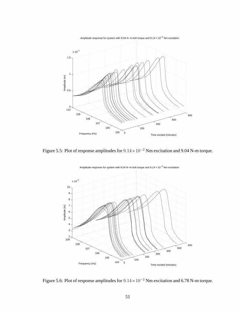
5.4, 5.5, 5.6, 5.7, 5.8, and5.9show the results from the tests. Figures5.10, 5.11, 5.12and

5.13show that as excitation time increased, the response amplitude of the system increased

for most cases.

This result demonstrates that the 4-6% drop in bolt tension has less affect on the dy-

namics than other phenomena that increase amplitude. If the drop in bolt tension were the

dominant effect then from Figure5.1 it would be assumed that the amplitude would drop.

The opposite is observed where the amplitude increases. This means that something more

dominant is happening to the system than the drop in bolt tension. It also appears that the

system responses have a reduced spring softening affect. It should be noted that when the

system sat unexcited the frequency response amplitude jumped both up and down, then

returned to level close to those from the day before.

50

0

200

400

600

800

105

106

107

108

109

1100

0.5

1

1.5

x 10−5



Frequency (Hz)

Am

plitu

de (

m)


0100

200300

400500

600

104

105

106

107

108

1092

3

4

5

6

7

8

9

10

x 10−6



Frequency (Hz)

Am

plitu

de (

m)


51

0

500

1000

1500

2000

107

108

109

110

111

1120

0.5

1

1.5

2

2.5

x 10−5



Frequency (Hz)

Am

plitu

de (

m)


0100

200300

400500

106

107

108

109

110

111

1120

0.5

1

1.5

2

2.5

x 10−5



Frequency (Hz)

Am

plitu

de (

m)


52

0100

200300

400500

104

105

106

107

108

109

1100

0.5

1

1.5

2

x 10−5



Frequency (Hz)

Am

plitu

de (

m)


0 50 100 150 200 250 300 350 4000.8

0.85

0.9

0.95

1

1.05

1.1

1.15

1.2

1.25

1.3x 10

−4

Time (minutes)

Am

plitu

de (

m)

Comparison of peak amplitudes vs. time at 4.57 × 10−2 Nm excitation

11.30 N−m9.04 N−m6.78 N−m

Figure 5.10:Plot of peak response amplitudes for4.57× 10−2 Nm excitation.

53

0 50 100 150 200 250 300 350 400 450 5000.8

0.9

1

1.1

1.2

1.3

1.4x 10

−4

Time (minutes)

Am

plitu

de (

m)

Comparison of peak amplitudes vs. time at 9.14 × 10−2 Nm excitation

11.30 N−m9.04 N−m6.78 N−m

Figure 5.11:Plot of peak response amplitudes for9.14× 10−2 Nm excitation.

0 50 100 150 200 250 300 350 400107

107.5

108

108.5

109

109.5

Time (minutes)

Fre

quen

cy (

Hz)

Frequencies of peak amplitudes vs. time at 4.57 × 10−2 Nm excitation

11.30 N−m9.04 N−m6.78 N−m

Figure 5.12:Plot of peak response frequencies for4.57× 10−2 Nm excitation.

54

0 50 100 150 200 250 300 350 400 450 500105.5

106

106.5

107

107.5

108

Time (minutes)

Fre

quen

cy (

Hz)

Frequencies of peak amplitudes vs. time at 9.14 × 10−2 Nm excitation

11.30 N−m9.04 N−m6.78 N−m

Figure 5.13:Plot of peak response frequencies for9.14× 10−2 Nm excitation.

5.2.3 Quantification of Damping Ratio and Natural Frequency

Non-linear Modeling

In order to compare how the system changes over the course of the experiment, model

identification was performed. It was desired for the parameters to represent commonly

understood dynamic features, like damping ratio and natural frequency. This model is

not supposed to be a predictive model, i.e. it is to be used as a metric for changes in the

system and may not to have the necessary complexity to consider the autonomous and

non-autonomous parameters in the system.

The experiment demonstrated a softening spring effect, but not drifting,. A cubic

stiffness nonlinearity matches this effect. The modes of the system are well isolated, so a

55

single degree of freedom model was adopted. Initial curve fits using the Duffing equation,

Equation5.1, did not give the desired results. The Duffing equation could fit the peak, but

lacked the ability to fit either side away from the peak. Cubic damping was added to the

Duffing equation giving Equation5.2.

x + 2ζωnx + kx + αx3 = U cos(Ωt) (5.1)

x + 2ζωnx + γx3 + kx + αx3 = U cos(Ωt) (5.2)

In order to solve for the steady state response of the system the method of harmonic

balance is used [16]. Harmonic balance expresses a periodic signal (Equation5.3). This

solution is substituted back into the governing differential equation and the coefficients of

each lowestM + 1 harmonics are set to zero.

x =M∑

m=0

am cos (mωt + mφ) (5.3)

The very narrowband-tracking filter used with the sine sweeps eliminates all but the

fundamental response frequency. This filtering justifies the use of a single term harmonic

balance solution to identify the damping ration and natural frequency. For the single term

case the phase shift is accounted for in the excitation giving

x + 2ζωnx + γx3 + kx + αx3 = U cos(Ωt + φ) (5.4)

56

with assumed solution

x = a cos(Ωt) (5.5)

Substituting equation5.5 into equation5.4and setting the coefficients ofsin(Ωt) and

cos(Ωt) equal to zero gives equations5.6and5.7

ω2n − Ω2 +

3

4αa2 =

U

acos(φ) (5.6)

−2ζΩωn −3

4γa2Ω3 =

U

asin(φ) (5.7)

Squaring the equations, adding them, then solving for the amplitudea yields six pos-

sible solutions. Three of those solutions are infeasible, as the amplitude for this system

is always positive. The remaining solutions are valid only for real values of amplitude.

The solution was found using Mathematica, and programmed into MATLAB to perform the

identification. The code containing the solution is presented in AppendixD.

It is important to note thata is a function ofΩ. The linear damping ratio,ζ, is a

measure of the energy dissipated from the system. The natural frequencyωn is the same as

if the system were linear,α = 0 Figure5.14. The non-linear coefficientα determines the

direction the backbone curves. It also determines the shape at the corner of the hysteresis

curve. When the system is spring softening, that isα < 0 as in Figure5.15, the amplitude

response curve looks like it leans to the left. The hysteresis loop also begins to bend at the

edges of the loop as Figures5.15and5.16demonstrate. The nonlinear damping termγ

adjusts the width of the response peak and height. It controls the shape of the amplitude

response plot in a very similar way that the linear damping ratio does.

57

−1 −0.8 −0.6 −0.4 −0.2 0 0.2 0.4 0.6 0.8 1−200

−150

−100

−50

0

50

100

150

200Hysteresis loop for linear system α = 0

Displacement

For

ce

Figure 5.14:Hysteresis loops from non-linear equation:α is zero.

−1 −0.8 −0.6 −0.4 −0.2 0 0.2 0.4 0.6 0.8 1−150

−100

−50

0

50

100

150Hysteresis loop for spring softening α <0

Displacement

For

ce

Figure 5.15:Hysteresis loops from non-linear equation: sign ofα is negative.

58

−1 −0.8 −0.6 −0.4 −0.2 0 0.2 0.4 0.6 0.8 1−250

−200

−150

−100

−50

0

50

100

150

200

250Hysteresis loop for spring hardening α >0

Displacement

For

ce

Figure 5.16:Hysteresis loops from non-linear equation: sign ofα is positive.

Identification of the Non-linear Differential Equation

The amplitude function can be used as a cost function to optimize the parametersωn, ζ,

γ, andα with known parametersa(Ω) andΩ. The phase,φ, is not used in finding the

amplitude of the response. MATLAB ’s optimization toolbox non-linear least squared error

curve fit routine was used to optimize the unknown parameters. AppendixD contains one

example routine for fitting data at 6.78 N-m.

A non-linear equation was used to curve fit each of the sine sweeps done to estimate

the parameters of the system (Section5.2.3). Particular interest was paid to the natural fre-

quency and the damping ratio. Figure5.17demonstrates a typical curve fit of the response

amplitude using the cubic damping and cubic stiffness nonlinear equation. The measured

59

106 106.5 107 107.5 108 108.5 109 109.5 110 110.5 1112

3

4

5

6

7

8

9

10

11x 10

−5

Frequency (Hz)

Am

plitu

de (

m)

Amplitude response at 0 min, 11.30 N−m torque, 9.14× 10−2 Nm excitation

Measured responseIdentifified response

Figure 5.17:Typical curve fit using least squares.

and identified fit well at the peak and along the higher frequency side, but separate on the

lower frequency side.

Natural Frequency

Figures5.18and5.19demonstrate that the natural frequency of the system did not notice-

ably change over time. The results obtained from changing the initial bolt torque indicate

the natural frequency should drop as the bolt tension is decreased. The reduction in tension

does not seem to be a major contributor to the changes seen in the response of the structure.

60

0 50 100 150 200 250 300 350 400 450 500106.5

107

107.5

108

108.5

109

Time excited (min)

ωn (

Hz)

Comparison of the natural frequency vs. time for 9.14 × 10−2 Nm excitation

11.30 N−m9.04 N−m6.78 N−m

Figure 5.18:Change inωn for 9.14× 10−2 Nm excitation.

0 50 100 150 200 250 300 350 400107.6

107.8

108

108.2

108.4

108.6

108.8

109

109.2

109.4

109.6

Time excited (min)

ωn (

Hz)

Comaprison of the natural frequency vs. time for 4.57 × 10−2 Nm excition

11.30 N−m9.04 N−m6.78 N−m

Figure 5.19:Change inωn for 4.57× 10−2 Nm excitation.

61

System Damping

Two damping terms are present in this model, non-linear cubic damping and linear damp-

ing. The original modeling used only the linear damping term to model the peaks, but

issues arose with getting the width of the peak to match the experimental data. The cubic

non-linear term was then added to account for this.

The linear damping ratio, shown in Figures5.20and5.21, is difficult to interpret. For

the9.14× 10−2 Nm excitation the damping ratio for the higher initial bolt torques appears

to drop, where as for the lowest bolt torque increases. When the non-linear damping ratios,

shown in Figures5.22 and5.23, are considered it becomes apparent that the linear and

non-linear terms are correlated to each other.

The lowest bolt torque for the9.14×10−2 Nm excitation case demonstrates this corre-

lation well. The linear damping starts low and increases, where as the non-linear ratio starts

high and drops. The other cases show this same behavior. Upon reviewing the cost function

used for curve fitting there seems to be a duality in the solution where either the non-linear

term is higher and the linear lower or visa-versa. The solution is highly dependent on the

initial guess for these parameters, leading to the jagged fits for the lower amplitude exci-

tation (Figures5.21and5.23). The non-linear term is necessary because results obtained

without the term did not converge to a solution that matched the data.

62

0 50 100 150 200 250 300 350 400 450 5000

1

2

3

4

5

6

7x 10

−3

Time excited (min)

ζ

Comparison of the damping ratio vs. time for 9.14 × 10−2 Nm excitation

11.30 N−m9.04 N−m6.78 N−m

Figure 5.20:Change inζ for 9.14× 10−2 Nm excitation.

0 50 100 150 200 250 300 350 4001

1.5

2

2.5

3

3.5

4x 10

−3

Time excited (min)

ζ

Comaprison of the damping ratio vs. time for 4.57 × 10−2 Nm excition

11.30 N−m9.04 N−m6.78 N−m

Figure 5.21:Change inζ for 4.57× 10−2 Nm excitation.

63

0 50 100 150 200 250 300 350 400 450 5000

500

1000

1500

2000

2500

3000

3500

4000

Time excited (min)

γ

Comprison of the cubic damping term vs. time for 9.14 × 10−2 Nm excitation

11.30 N−m9.04 N−m6.78 N−m

Figure 5.22:Change in cubic damping coefficient,γ, for the9.14× 10−2 Nm excitation.

0 50 100 150 200 250 300 350 4000

100

200

300

400

500

600

700

800

Time excited (min)

γ

Comaprison of the cubic damping term vs. time for 4.57 × 10−2 Nm excition

11.30 N−m9.04 N−m6.78 N−m

Figure 5.23:Change in cubic damping coefficient,γ, for the4.57× 10−2 Nm excitation.

64

Non-linear Stiffness

From a visual examination of Figure5.1 it might be assumed that as the bolt tension is

reduced the system non-linearity becomes softer. That is, the non-linear coefficient would

have a greater magnitude with negative sign. Figure5.25 and5.24 demonstrate that the

non-linear coefficient does not follow this trend. Thoughα for the 6.78 N-m case has the

greatest negative magnitude, the 11.30 N-m case does not have the smallest negative value

for 9.14× 10−2 Nm excitation.

The model may not have the accuracy to compare between excitation levels. It would

be expected that the initial sine sweep for each torque level should curve fit almost the

same. The curve fit of the 11.30 N-m bolt torque for9.14× 10−2 Nm and4.57× 10−2 Nm

differ by 70% initially.

65

0 50 100 150 200 250 300 350 400 450 500−14

−13

−12

−11

−10

−9

−8

−7

−6

−5x 10

11

Time excited (min)

α

Comparison of α vs. time for 9.14 × 10−2 Nm excitation

11.30 N−m9.04 N−m6.78 N−m

Figure 5.24:Change inα for the9.14× 10−2 Nm excitation.

0 50 100 150 200 250 300 350 400−9

−8

−7

−6

−5

−4

−3

−2x 10

11

Time excited (min)

α

Comaprison of the non−linear stifness coefficient vs. time for 4.57 × 10−2 Nm excition

11.30 N−m9.04 N−m6.78 N−m

Figure 5.25:Change inα for the4.57× 10−2 Nm excitation.

66

5.3 Hysteresis loops

A study was done to consider the change in the shape of the hysteresis loop based on

torque, time, frequency, and excitation level. The specimen was cleaned before the test

started. The torque levels and excitation levels were the same used for the sine dwell and

sweep tests (Section5.2). Unlike those tests, intermediate recordings during sine dwell

were not taken. That is, data was only taken at the beginning of the test and at the end of

the test. The vertical-direction acceleration and strain data were recorded from the top of

the flange. Data was also recorded from the lower flange strain gage and the upper strain

gage on the un-flanged side.

A sine sweep was performed from 110 Hz to 120 Hz using the same setup as Section

5.2. The sine sweep took 40-minutes to complete. Following the sweep the structure was

set to dwell at resonance with the same excitation used for the sweep. Five thousand time

averages were recorded. Another time history was recorded at 65 Hz. This frequency was

chosen based on isolation from system support interactions (See Section3.2). Interference

from lights or supplied electricity (120 Hz and 60 Hz) was insignificant. The frequency

was sufficiently far away from system resonances to make the low amplitude non-linear

phenomena observable.

A resonant frequency sine dwell was also recorded, though the amplitude of the re-

sponse made observing the non-linearly excited harmonics difficult. the system is allowed

to dwell for 36 hours, then another set of impact, sweeps, and dwells are recorded. For

analysis the measured strain from the specimen mounted strain gages was used to find mo-

ment collocated with the acceleration measured. The acceleration was integrated twice to

67

−6 −4 −2 0 2 4 6

x 10−5

−0.25

−0.2

−0.15

−0.1

−0.05

0

0.05

0.1

0.15

0.2

0.25

Hysteresis curve at 65 Hz with 6.78 N−m bolt torque and 4.57 × 10−2 Nm excitation

Displacement (m)

Mom

ent (

N−

m)

(a) Hysteresis away from resonance

−6 −4 −2 0 2 4 6

x 10−5

−0.25

−0.2

−0.15

−0.1

−0.05

0

0.05

0.1

0.15

0.2

0.25

Hysteresis curve at resonance with 6.78 N−m bolt torque and 4.57 × 10−2 Nm excitation

Displacement (m)

Mom

ent (

N−

m)

(b) Hysteresis at resonance

Figure 5.26:Hysteresis curves at 65 Hz and resonance are not comparable.

indicate the displacement of the system.

A direct comparison between loops taken at resonance and loops taken at 65 Hz is

difficult, as shown in Figure5.26. For this reason the results will be presented based on

frequency of excitation and broken down further based on excitation level.

5.3.1 Hysteresis curves at resonance

It was hoped that results taken at resonance would show non-linear harmonics and an in-

crease in energy dissipation because of the large response amplitude. This was not the case.

In Figure5.27the hysteresis curves are dominated by the primary resonant frequency ob-

scuring the non-linear effects of the system. However, these results do indicate a reduced

amplitude response with reduced initial bolt torque. This is in agreement with the bolt

torque frequency sweeps taken separately.

68

−6 −4 −2 0 2 4 6 8

x 10−5

−0.4

−0.3

−0.2

−0.1

0

0.1

0.2

0.3

Displacement (m)

Mom

ent (

N−

m)

Hysteresis curves at resonance with 6.78 N−m bolt torque and 4.57 × 10−2 Nm excitation

ReconstitutedRelaxed

(a) Lower excitation, 6.78 N-m bolt torque.

−1 −0.8 −0.6 −0.4 −0.2 0 0.2 0.4 0.6 0.8 1

x 10−4

−0.5

−0.4

−0.3

−0.2

−0.1

0

0.1

0.2

0.3

0.4

0.5

Displacement (m)

Mom

ent (

N−

m)



(b) Higher excitation, 6.78 N-m bolt torque.

−1 −0.8 −0.6 −0.4 −0.2 0 0.2 0.4 0.6 0.8 1

x 10−4

−0.4

−0.3

−0.2

−0.1

0

0.1

0.2

0.3

0.4

Displacement (m)

Mom

ent (

N−

m)



(c) Lower excitation, 9.04 N-m bolt torque.

−1.5 −1 −0.5 0 0.5 1 1.5

x 10−4

−0.8

−0.6

−0.4

−0.2

0

0.2

0.4

0.6

Displacement (m)

Mom

ent (

N−

m)



(d) Higher excitation, 9.04 N-m bolt torque.

−1 −0.8 −0.6 −0.4 −0.2 0 0.2 0.4 0.6 0.8 1

x 10−4

−0.5

−0.4

−0.3

−0.2

−0.1

0

0.1

0.2

0.3

0.4

0.5

Displacement (m)

Mom

ent (

N−

m)



(e) Lower excitation, 10.3 N-m bolt torque.

−1.5 −1 −0.5 0 0.5 1 1.5

x 10−4

−0.8

−0.6

−0.4

−0.2

0

0.2

0.4

0.6

0.8

Displacement (m)

Mom

ent (

N−

m)



(f) Higher excitation, 10.3 N-m bolt torque.

Figure 5.27:Subtle features are hidden in the hysteresis curves at resonance.

69

5.3.2 Hysteresis curves at 65 Hz

The curves recorded at 65Hz are different in appearance than those at resonance. The

hysteresis curves at4.57×10−2 Nm excitation, Figures5.28, 5.30, and5.32, have a crescent

like shape. The hysteresis curves at9.14 × 10−2 Nm, Figures5.29, 5.31, and5.33, excite

an additional frequency. This non-linearly excited frequency correlates to the fifth bending

mode, shown in Figure2.6.

The hysteresis curves from 6.78 N-m of bolt torque, Figures5.28and5.29, show a

clockwise rotation in the hysteresis curve. The clockwise rotation denotes that for the same

input more output is measured. At 9.04 N-m this changes to a slight counter clockwise

rotation (Figures5.30and5.31). When the bolt was given a torque of 11.30 N-m there was

no noticeable rotation in the hysteresis curve (Figures5.32and5.33).

Again, the results here do not contradict results from other experiments in this thesis.

The displacements between bolt torque levels do not change by much, but this is to be

expected since the specimen is being excited away from resonance. The introduction of

harmonics from single sine excitation indicates a non-linear system.

5.4 Qualitative Observations

The response amplitude of the jointed specimen at the first resonance was not perceivable

to the naked eye. The vibration of the specimen at this resonance could be felt. If the

specimen were in close proximity to the naked ear (within a foot) and the excitation was

greater than6.85 × 10−2 Nm then an audible hum could be heard. This is a noticeable

70

−1 −0.8 −0.6 −0.4 −0.2 0 0.2 0.4 0.6 0.8 1

x 10−6

−1.5

−1

−0.5

0

0.5

1

1.5x 10

−3

Displacement (m)

Mom

ent (

N−

m)

Hysteresis curves at 65 Hz with 6.78 N−m bolt torque and 4.57 × 10−2 Nm excitation


Figure 5.28:Hysteresis at 65 Hz with4.57× 10−2 Nm excitation and 6.78 N-m torque.

−2 −1.5 −1 −0.5 0 0.5 1 1.5 2

x 10−6

−2.5

−2

−1.5

−1

−0.5

0

0.5

1

1.5

2

2.5x 10

−3

Displacement (m)

Mom

ent (

N−

m)




71

−1 −0.8 −0.6 −0.4 −0.2 0 0.2 0.4 0.6 0.8 1

x 10−6

−1.5

−1

−0.5

0

0.5

1

1.5x 10

−3

Displacement (m)

Mom

ent (

N−

m)




−2 −1.5 −1 −0.5 0 0.5 1 1.5 2

x 10−6

−2.5

−2

−1.5

−1

−0.5

0

0.5

1

1.5

2

2.5x 10

−3

Displacement (m)

Mom

ent (

N−

m)




72

−1 −0.8 −0.6 −0.4 −0.2 0 0.2 0.4 0.6 0.8 1

x 10−6

−1.5

−1

−0.5

0

0.5

1

1.5x 10

−3

Displacement (m)

Mom

ent (

N−

m)


RecontsitutedRelaxed


−2 −1.5 −1 −0.5 0 0.5 1 1.5 2

x 10−6

−2.5

−2

−1.5

−1

−0.5

0

0.5

1

1.5

2x 10

−3

Displacement (m)

Mom

ent (

N−

m)




73

difference from the response of the control specimen. The jointed specimen did not appear

to rock or swing while being excited by the piezoelectric patches, and the support wires felt

still.

Depending on the level and frequency of excitation the thin flanges appeared to flap

away from the tongued portion, then slap against it. This phenomenon was not perceivable

at the frequencies used for testing the specimen. The compliance of the flanges also made

joint assembly more difficult. The assembly was visually inspected to make sure the joint

had been tightened without inadvertently bending the flanges. The bolt tension from using

the calibrated torque method was very dependent on the flange fastening position.

When the joint was separated a coating of metal dust was present between the tongue

and flanges. When cleaned using brake cleaner, the surface was polished and pitted (Figures

5.35& 5.34). The polishing and pitting was not visible when first machined.

The wear in the center of the surfaces might be from a small ridge on the inside of

the flanges. This ridge was formed during manufacturing, though it wasn’t noticed until

shortly after initial experiments began.

74

Figure 5.34:Wear patterns down the center of the flanges and scratching/polishing marks

from washers.

75

Figure 5.35:Polishing and pitting on one side of the tongue.

76

Conclusions

6.1 Joint Dynamics

Several experiments to characterize the dominant dynamic affects of adding a bolted joint

have been performed. A control specimen and a jointed specimen were tested. Two types

of tests were done. Frequency sweeps were performed to look at the effect of the joint in

the frequency domain and hysteresis curves were taken to examine the energy dissipated

per cycle. The difference in the response between the two specimens was attributed to the

effect of the bolted joint.

The effect of initial bolt tension can be a major factor in joint behavior. The resonant

frequency of the first bending mode shifted to a lower frequency as the initial bolt tension

was reduced. Bolt tension dropped as the system was excited. The bolt tension reduced

quickly just after tightening. This drop could be attributed to many different phenomena

like embedding and creep though no particular phenomena have been isolated. This reduc-

tion does not appear to be the dominant effect in the dynamics of the system. In some cases

the response amplitude increased 11-16% yet the bolt tension decreased up to 6%.

77

Two possibilities exist for this increase in magnitude. The first is a reduction in the

softening effect, effectively unbending the peak. The second is a decrease in the damping of

the joint. It could be reasoned that the linear stiffness could change but this term is directly

related to linear system natural frequency, which does not change. The curve fit data using

cubic damping and cubic stiffness does seem to suggest both the damping decrease and a

softening effect decrease, but the results are unreliable.

Initial conditions made curve fitting difficult. Many local minima existed making it

difficult to achieve a consistent solution. It also appears that the linear and non-linear

damping coefficients are correlated to each other. When one is identified as lower, the

other is identified as higher. The system non-linearity appears to need more or different

terms than cubic stiffness and cubic damping to describe them.

From sine dwell hysteresis curves its evident the joint response does not behave in a

manner predicted by joint models. The loops appear to be spring hardening in positive dis-

placement and spring softening in negative displacement. the control specimen exhibited

strange hysteretic behavior. The first time data was taken the system exhibited a tri-linear

response, then when the system was literally flipped over and testing again the tri-linear re-

gion disappeared. It’s unclear why this happened, as is unclear why the jointed specimen’s

hysteresis looks like a crescent.

78

6.2 Future Work

The initial thrust of this work was to adapt a joint model for non-deterministic approaches

in predicting dynamic motion in bolted joints. This goal was not feasible with the current

models found in the cited literature. More basic research needs to be performed to un-

derstand the physics involved at the joint interface. Finite elements can help but only in

limited ways. A highly refined mesh of the joint element can give insight into the effect of

geometry. Finite elements programs are limited in that they cannot accurately model the

pitting and polishing seen in the experiment. Additional lab testing will need to be done.

If a model could capture the physics with some consistency then the original purpose

of this work can be continued. Several washers were to be used as new joint surfaces. It

is advised that this testing be automated. The automation would keep testing consistent

between trials. Consistency would reduce operator variability. If a joint model were able

to capture the dynamics of the joint, then its parameters could be identified and used as a

metric. The statistical basis for the variability would be based on these identified parame-

ters.

79

Bibliography

[1] Iwan, W. D., “A Distributed-Element Model for Hysteresis and Its Steady-State Dy-

namic Response,”Journal of Applied Mechanics, Vol. 33, 1966, pp. 893–900.

[2] Shiryayev, O. V., Page, S. M., Pettit, C. L., and Slater, J. C., “Parameter Identification

and Investigation of a Bolted Joint Model,” To Appear in the Journal of Sound and

Vibration.

[3] Yue, X.,Developments of Joint Elements and Solution Algorithims for Dynamic Anal-

ysis of Jointed Structures, Ph.D. thesis, University of Colorado, 2002.

[4] Segalman, D. J., “A Four-Parameter Iwan Model for Lap-Type Joints,” Tech. Rep.

SAND-2002-3828, Sandia National Laboratories, November 2002.

[5] Song, Y., Hartwigsen, C. J., McFarland, D. M., Vakakis, A. F., and Bergman, L. A.,

“Simulation of Dynamics of Beam Structures with Bolted Joints Using Adjusted Iwan

Beam Elements,”Journal of Sound and Vibration, Vol. 273, 2004, pp. 249–276.

[6] Wen, Y. K., “Method for Random Vibration of Hysteretic Systems,”Journal of Engi-

neering Mechanics, Vol. 102-EM2, 1976, pp. 249–263.

[7] de Wit, C. C., Ollson, H.,Astrom, K. J., and Liscinsky, P., “A New Model for Control

of Systems with Friction,”IEEE Transactions on Automatic Control, Vol. 40, No. 3,

1995.

80

[8] Norton, R. L., Machine Design an Integrated Approach, chap. 14, Prentice-Hall,

2000, pp. 875–940.

[9] Pai, N. G. and Hess, D. P., “Experimental Study of Loosening of Threaded Fasteners

Due to Dynamic Shear Loads,”Journal of Sound and Vibration, Vol. 253, No. 3, 2002,

pp. 585–602.

[10] Bickford, J. H.,An Introduction to the Design and Behavior of Bolted Joints, New

York: Marcel Dekker, 3rd ed., 1995.

[11] Jiang, Y., Zhang, M., and Lee, C.-H., “A Study of Early Stage Self-Loosening of

Bolted Joints,”Transactions of the ASME, Vol. 125, September 2003, pp. 518–526.

[12] Basava, S. and Hess, D. P., “Bolted Joint Clamping Force Variation Due to Axial

Vibration,” Journal of Sound and Vibration, Vol. 210, No. 2, 1998, pp. 255–265.

[13] Dosch, J. J., Inman, D. J., and Garcia, E., “A Self-Sensing Piezoelectric Actuator for

Collocated Control,”Journal of Intelligent Material Systems and Structures, Vol. 3,

1992, pp. 166–185.

[14] Chladni, E.,Entdeckungenuber die Theroie des Klanges., Weidmanns Erban und

Reich, Leipzig, 1787.

[15] Keller, T., “On the Use of Tracking Filters During Sine Vibration Testing,”Sound and

Vibration, Vol. 36, No. 1, 2002, pp. 82–85.

[16] Nayfeh, A. H. and Mook, D. T.,Nonlinear Oscillations, John Wiley & Sons, Inc.,

1979.

81

Preparing Specimen

To insure accurate, repeatable measurements the test specimen needs to be configured in

a systematic fashion. This procedure focuses on the setup of the bolt-equipped appara-

tus, though the single piece structure is similar. Setting up the structure begins with the

collection of the necessary parts, assembling the structure, and an initial test for proper

assembly.

A.1 Collect Parts

Make sure the following instrumentation and parts are available

1. computer with DAQ

2. strain gage amplification systems

3. piezoelectric patch/accelerometer amplifiers

4. instrumented bolt

5. labeled washers and nut

6. both halves of instrumented jointed specimen

7. test frame

8. stainless steel wire

82

9. specimen stand

10. misc. wiring

A.2 Assemble Specimen

Prior to assembly it is assumed that all transducers were calibrated and that the sensitivities

are known. It is also assumed that transducers have been applied. If not see appendixC.

1. Clean a work area large enough to work with the test specimen. Examine the trans-

ducers and wires for any physical damage or looseness. Make sure that all transducer

wires are secured. Move the two pieces of the test specimen together so that the lap

joint can be secured with a bolt. the integral masses should rest on a stand so that the

specimen can be hung with little movement.

2. Put 1 washer onto the instrumented bolt and insert the bolt into the lap joint. Put a

washer followed by a nut on the exposed thread of the bolt and run the nut up to the

specimen.DO NOTcinch the nut. The bolt should be able to ‘jiggle’ in the joint.

3. Make a ‘splint’ for the joint. Put one piece of flat stock on each side (parallel to

hole) of the joint and hold with 2 clamps. Use caution to not rub, scrape, or pull the

transducers or their wires.

4. Balance the strain gage amplifiers. Make sure the bolt is still loose enough to not

bias the load.

5. Hold thehead of the boltwith a wrench while using a torque wrench to tighten the

nut. The head should remain stationary while the nut is rotated.Do not exceed 20

lbs-ft of torque.Apply the predetermined torque. Let the system set for 3-4 seconds,

loosen nut and re-tighten.

6. Hang the specimen buy looping stainless steel line around mounting bolts and through

test frame. Attach any remaining transducers, and connect all the instrumentation to

83

the equipment. Try to isolate wires from noise sources and secure them to avoid

vibration during testing.

7. remove the supports used to hold up the specimen. It should hang freely. Check to

make sure the specimen is electrically isolated. Make sure all the equipment is on

and has warmed up.

A.3 Testing the Installation

At this point the test rig and specimen are ready to be tested for proper installation.

1. Start the DAQ system and check for signals on all connected channels. Look at each

channel and determine if the signal is appropriate, i.e. there are no unexplained spikes

or bias voltages for the current conditions.

2. Input a signal1 to the piezoelectric patches and check that the strain gages on the

specimen detect the change.

3. If wires have been moved or put on for the first time check to see that their effect has

been minimized. Do this by loosening the wire and exciting the system at resonance.

hold the wire between your fingers at different locations and compare the resulting

amplitude. Locations with higher amplitudes have less damping and are desirable.

Now look for locations to fix the wire too.

4. Use the measured load from the bolt and compare with the estimated torque load.

AppendixB has the associated data and equations.

5. If everything makes sense and checks out then the experimentation begins.

1Only do steps2 and3 if the time history is not important for that run.

84

Torque to preload calculations

TableB.2 has the properties of aluminum needed to calculate the load.µ is listed for Al

on Al contact. FigureB.1 shows the dimensions needed and TableB.1 has dimensions for

1/2-20 UNF thread.

Figure B.1:Thread dimensions illustrated.

The equation for estimated torque from a desired load is shown inB.

T =

[(dm

2d

) (tan λ + µ sec α

1 − µ tan λ sec λ

)+ 0.625 µc

]Fi d (B.1)

µc andµ represent the coefficient of friction between the head and body and the bolt and

nut threads, respectively. Since this test case has only one material,µc = µ. Often the

Table B.1:Dimension information for 1/2-20 UNF thread.

d 0.500 in

dm 0.4374 in

P 0.050 in

α 30

λ 2.08

85

Table B.2:material properties of AL 7075-T7351.

E (Young’s Modulus) 72 GPa

σy 435 MPa

D (Density) 2810 Kg/m3

µ (Coeff. of friction) 0.40

majority of equationB is given the variableK because standard thread sizes have uniform

values.K andT are then given as

K =

(dm

2d

) (tan λ + µ sec α

1 − µ tan λ sec λ

)+ 0.625 µc

T = KFid (B.2)

Since the data used forµ has been estimated from uncertain Internet sources, it would

be advisable to figure out the preload and estimate theK value for the system. It is also

important to realize that the equation for torque to load is an estimate. The bolt torque

method has been found to be off as much as±40%.

86

Application of transducers

Heisenberg was a German scientist who worked with quantum mechanics. He made a

principle involving atoms stating “The more precisely the position is determined, the less

precisely the momentum is known in this instant, and vice versa.” Every piece of equip-

ment added to a test article changes it’s dynamics, making the measurement not the system

in question, but the modified system. The best method for measurements requires instru-

mentation that does not change the system. This is either impractical or impossible, so

methods have been introduced to reduce instrumentation impact and maintain precision.

C.1 Foil strain gages

Application of foil strain gages can be a tedious procedure. If care is taken then the gage

life will be lengthened and its precision will be maintained. A recommended procedure

exists in Bulletin 309D from Measurement Group. Gages are tested after installation for

isolation and proper resistance. The use of M-bond glue dictates a max life span for the

gage installation of one year.

C.2 Piezoelectric Patches

Piezoelectric patches were purchased from Ferro-perm for exciting the structure. They

measure 2.54 cm x 2.54 cm x 0.05 cm using material type Pz-29. To make the installation

87

more uniform a simple jig was used. The jig was machined on a vertical mill to space the

edge of the piezoelectric patch 2 inches from the closest integral mass.

The patches were attached to the structure using CircuitWorks®Conductive Epoxy,

a product made by Chemtronics®. The epoxy is designed for high strength conductive

bonding. During installation a hot air based paint stripper was used to heat the surround-

ing structure. The aluminum conducted the heat to the epoxy. In this manner the epoxy

set faster, harder, and with optimal conductivity but without damaging the piezoelectric

patches.

The patches were installed with the positive face exposed on the top and bottom of

the beam. When exciting the extensional frequency the patches were in parallel and the

voltage dropped across both upper and lower patches was equal to the excitation voltage.

When exciting the beam in bending, the patches were put into series

C.3 Piezoelectric Strain Gages

PCB model 740B02 strain gages were applied at 4 locations on the test specimen. They

were positioned so as to measure the axial strain in the specimen at almost the same location

as the accelerometers were measuring acceleration. The specimen was prepared by sanding

the surface with 400 grit sandpaper. The surface was then cleaned using common brake

cleaner. This removed all the surface oils and particles from sanding. Using a ruler and

straight edge a rectangle was drawn where the transducer was going to be mounted.

A piece of clear tape was placed over the sensor, with over an inch of tape over hanging

the sensor. Loctite 420 was applied to the sensor and a razor blade was used to smooth the

glue over the bottom of the sensor. The sensor was lined up with the previously made

rectangle and pressed down. The tape was used to secure the transducer while the glue

cured.

After 8 hours the sensor was tested for conductivity to the specimen. If the resistance

was greater than 10 MΩ the sensor was considered successfully installed. If not the senor

88

was removed and the process repeated.

C.4 Piezoelectric Accelerometers

PCB accelerometers models 356A16 and 356A24 were mounted in 4 locations, physically

close to 4 strain gages. The mounting for the accelerometers is the similar to the process

described for the strain gages in AppendixC.3 but the surface of the specimen was not

sanded.

89

Appendix D

Coded Harmonic Balance

Function for amplitude response: “har3.m”%Harmonic balance 3 (har3) uses a 1 term harmonic balance solution to the%SDOF GDEQ with both cubic damping and Cubic stiffness. This file is%intended to be used with a non-linear least squares curve fit routine.

function amp =har3(par,o)

w=par(1) * 1e2;z=par(2) * 1e-3;al=par(3) * 1e11;g=par(4)P=par(5) * 1e-2;

%The soultion uses a lot of repetitous code. To reduce number crunching%these repetitions have been labeled at p1, p1a, p2 and are used in%the following code.p1=alˆ2+gˆ2 * o.ˆ6;

p1a=-3456 * alˆ3 * o.ˆ6 - 31104 * al * gˆ2 * o.ˆ12 + 34992 * alˆ4 * Pˆ2 + ...69984 * alˆ2 * gˆ2 * o.ˆ6 * Pˆ2 + 34992 * gˆ4 * o.ˆ12 * Pˆ2 + 10368 * alˆ3 * o.ˆ4 * wˆ2 + ...93312 * al * gˆ2 * o.ˆ10 * wˆ2 - 10368 * alˆ3 * o.ˆ2 * wˆ4 - 93312 * al * gˆ2 * o.ˆ8 * wˆ4 + ...3456 * alˆ3 * wˆ6 + 31104 * al * gˆ2 * o.ˆ6 * wˆ6 - 103680 * alˆ2 * g* o.ˆ8 * w* z + ...62208 * gˆ3 * o.ˆ14 * w* z + 207360 * alˆ2 * g* o.ˆ6 * wˆ3 * z - 124416 * gˆ3 * o.ˆ12 * wˆ3 * z - ...103680 * alˆ2 * g* o.ˆ4 * wˆ5 * z + 62208 * gˆ3 * o.ˆ10 * wˆ5 * z - 124416 * alˆ3 * o.ˆ4 * wˆ2 * zˆ2 + ...207360 * al * gˆ2 * o.ˆ10 * wˆ2 * zˆ2 + 124416 * alˆ3 * o.ˆ2 * wˆ4 * zˆ2 - ...207360 * al * gˆ2 * o.ˆ8 * wˆ4 * zˆ2 + 248832 * alˆ2 * g* o.ˆ6 * wˆ3 * zˆ3 + ...27648 * gˆ3 * o.ˆ12 * wˆ3 * zˆ3;

p2=(p1a+(p1a.ˆ2+4 * (-576 * (al * o.ˆ2-al * wˆ2-2 * g* o.ˆ4 * w* z).ˆ2 ...+ 432 * (p1). * (o.ˆ4-2 * o.ˆ2 * wˆ2+wˆ4+4 * o.ˆ2 * wˆ2 * zˆ2)).ˆ3).ˆ(1/2)).ˆ(1/3);

%Amplitude is determined from a sixth order polynomial, which breaks down%to 3 possible solutions (amplitude is positive, eliminating 3 solutions)

a1=sqrt (8 * al * o.ˆ2./(9 * p1) - 8 * al * wˆ2./(9 * p1) - 16 * g* o.ˆ4 * w* z./(9 * p1)...+ 16* 2ˆ(1/3) * alˆ2 * o.ˆ4./(3 * p1. * p2)...- 16 * 2ˆ(1/3) * gˆ2 * o.ˆ10./(p1. * p2) ...- 32 * 2ˆ(1/3) * alˆ2 * o.ˆ2 * wˆ2./(3 * p1. * p2) ...+ 32* 2ˆ(1/3) * gˆ2 * o.ˆ8 * wˆ2./(p1. * p2) ...+ 16* 2ˆ(1/3) * alˆ2 * wˆ4./(3 * p1. * p2) ...

90

- 16 * 2ˆ(1/3) * gˆ2 * o.ˆ6 * wˆ4./(p1. * p2) ...- 256 * 2ˆ(1/3) * al * g* o.ˆ6 * w* z./(3 * p1. * p2) ...+ 256 * 2ˆ(1/3) * al * g* o.ˆ4 * wˆ3 * z./(3 * p1. * p2) ...- 64 * 2ˆ(1/3) * alˆ2 * o.ˆ2 * wˆ2 * zˆ2./(p1. * p2) ...+ 64* 2ˆ(1/3) * gˆ2 * o.ˆ8 * wˆ2 * zˆ2./(3 * p1. * p2) ...+ (p2)./(27 * 2ˆ(1/3) * p1));

a2=sqrt (8 * al * o.ˆ2./(9 * p1) - 8 * al * wˆ2./(9 * p1) - 16 * g* o.ˆ4 * w* z./(9 * p1)...- (8 * 2ˆ(1/3) * alˆ2 * o.ˆ4)./(3 * p1. * p2) ...+ (8 * i * 2ˆ(1/3) * alˆ2 * o.ˆ4)./( sqrt (3) * p1. * p2)...+ (8 * 2ˆ(1/3) * gˆ2 * o.ˆ10)./(p1. * p2) ...- (8 * i * 2ˆ(1/3) * sqrt (3) * gˆ2 * o.ˆ10)./(p1. * p2) ...+ (16 * 2ˆ(1/3) * alˆ2 * o.ˆ2 * wˆ2)./(3 * p1. * p2) ...- (16 * i * 2ˆ(1/3) * alˆ2 * o.ˆ2 * wˆ2)./( sqrt (3) * p1. * p2) ...- (16 * 2ˆ(1/3) * gˆ2 * o.ˆ8 * wˆ2)./(p1. * p2) ...+ (16 * i * 2ˆ(1/3) * sqrt (3) * gˆ2 * o.ˆ8 * wˆ2)./(p1. * p2) ...- (8 * 2ˆ(1/3) * alˆ2 * wˆ4)./(3 * p1. * p2) ...+ (8 * i * 2ˆ(1/3) * alˆ2 * wˆ4)./( sqrt (3) * p1. * p2) ...+ (8 * 2ˆ(1/3) * gˆ2 * o.ˆ6 * wˆ4)./(p1. * p2) ...- (8 * i * 2ˆ(1/3) * sqrt (3) * gˆ2 * o.ˆ6 * wˆ4)./(p1. * p2) ...+ (128 * 2ˆ(1/3) * al * g* o.ˆ6 * w* z)./(3 * p1. * p2) ...- (128 * i * 2ˆ(1/3) * al * g* o.ˆ6 * w* z)./( sqrt (3) * p1. * p2) ...- (128 * 2ˆ(1/3) * al * g* o.ˆ4 * wˆ3 * z)./(3 * p1. * p2) ...+ (128 * i * 2ˆ(1/3) * al * g* o.ˆ4 * wˆ3 * z)./( sqrt (3) * p1. * p2) ...+ (32 * 2ˆ(1/3) * alˆ2 * o.ˆ2 * wˆ2 * zˆ2)./(p1. * p2) ...- (32 * i * 2ˆ(1/3) * sqrt (3) * alˆ2 * o.ˆ2 * wˆ2 * zˆ2)./(p1. * p2) ...- (32 * 2ˆ(1/3) * gˆ2 * o.ˆ8 * wˆ2 * zˆ2)./(3 * p1. * p2) ...+ (32 * i * 2ˆ(1/3) * gˆ2 * o.ˆ8 * wˆ2 * zˆ2)./( sqrt (3) * p1. * p2) ...- p2./(54 * 2ˆ(1/3) * p1) ...- i * p2./(18 * 2ˆ(1/3) * sqrt (3) * p1));

a3=sqrt (8 * al * o.ˆ2./(9 * p1) - 8 * al * wˆ2./(9 * p1) - 16 * g* o.ˆ4 * w* z./(9 * p1)...- (8 * 2ˆ(1/3) * alˆ2 * o.ˆ4)./(3 * p1. * p2) ...- (8 * i * 2ˆ(1/3) * alˆ2 * o.ˆ4)./( sqrt (3) * p1. * p2)...+ (8 * 2ˆ(1/3) * gˆ2 * o.ˆ10)./(p1. * p2) ...+ (8 * i * 2ˆ(1/3) * sqrt (3) * gˆ2 * o.ˆ10)./(p1. * p2) ...+ (16 * 2ˆ(1/3) * alˆ2 * o.ˆ2 * wˆ2)./(3 * p1. * p2) ...+ (16 * i * 2ˆ(1/3) * alˆ2 * o.ˆ2 * wˆ2)./( sqrt (3) * p1. * p2) ...- (16 * 2ˆ(1/3) * gˆ2 * o.ˆ8 * wˆ2)./(p1. * p2) ...- (16 * i * 2ˆ(1/3) * sqrt (3) * gˆ2 * o.ˆ8 * wˆ2)./(p1. * p2) ...- (8 * 2ˆ(1/3) * alˆ2 * wˆ4)./(3 * p1. * p2) ...- (8 * i * 2ˆ(1/3) * alˆ2 * wˆ4)./( sqrt (3) * p1. * p2) ...+ (8 * 2ˆ(1/3) * gˆ2 * o.ˆ6 * wˆ4)./(p1. * p2) ...+ (8 * i * 2ˆ(1/3) * sqrt (3) * gˆ2 * o.ˆ6 * wˆ4)./(p1. * p2) ...+ (128 * 2ˆ(1/3) * al * g* o.ˆ6 * w* z)./(3 * p1. * p2) ...+ (128 * i * 2ˆ(1/3) * al * g* o.ˆ6 * w* z)./( sqrt (3) * p1. * p2) ...- (128 * 2ˆ(1/3) * al * g* o.ˆ4 * wˆ3 * z)./(3 * p1. * p2) ...- (128 * i * 2ˆ(1/3) * al * g* o.ˆ4 * wˆ3 * z)./( sqrt (3) * p1. * p2) ...+ (32 * 2ˆ(1/3) * alˆ2 * o.ˆ2 * wˆ2 * zˆ2)./(p1. * p2) ...+ (32 * i * 2ˆ(1/3) * sqrt (3) * alˆ2 * o.ˆ2 * wˆ2 * zˆ2)./(p1. * p2) ...- (32 * 2ˆ(1/3) * gˆ2 * o.ˆ8 * wˆ2 * zˆ2)./(3 * p1. * p2) ...- (32 * i * 2ˆ(1/3) * gˆ2 * o.ˆ8 * wˆ2 * zˆ2)./( sqrt (3) * p1. * p2) ...- p2./(54 * 2ˆ(1/3) * p1) ...+ i * p2./(18 * 2ˆ(1/3) * sqrt (3) * p1));

%Amplitude is also real, so not all of these solutions are valid for the%responce frequencies used.

z1= find ( imag (a1)<=0.0000001 & imag (a1)>=-0.0000001);z2= find ( imag (a2)<=0.0000001 & imag (a2)>=-0.0000001);z3= find ( imag (a3)<=0.0000001 & imag (a3)>=-0.0000001);

%initialize amplitude arrayamp=zeros ( size (o));

%fill array with possible solutionsamp(z1)=a1(z1);amp(z2)=a2(z2);

91

amp(z3)=a3(z3);

Script for curve fitting amplitude response: “data60.m”file=[’ 60inlbs_1day_0min.vss’;

’ 60inlbs_1day_10min.vss’;’ 60inlbs_1day_20min.vss’;’ 60inlbs_1day_32min.vss’;’ 60inlbs_1day_48min.vss’;’ 60inlbs_1day_58min.vss’;’ 60inlbs_1day_68min.vss’;’ 60inlbs_1day_80min.vss’;’ 60inlbs_7day_0min.vss’;’ 60inlbs_7day_30min.vss’;’ 60inlbs_7day_140min.vss’;’ 60inlbs_8day_0min.vss’;’ 60inlbs_8day_38min.vss’;’ 60inlbs_8day_68min.vss’;’ 60inlbs_8day_113min.vss’;’ 60inlbs_14day_0min.vss’;’ 60inlbs_14day_60min.vss’;’ 60inlbs_15day_0min.vss’;’ 60inlbs_15day_62min.vss’;’60inlbs_15day_122min.vss’;’60inlbs_15day_182min.vss’;’ 60inlbs_16day_0min.vss’];

T=[0 10 20 32 48 58 68 80 80.1 110 220 220.1 258 288 333 333.1 393 393.1 455 515 575 575.1];

ub=[];lb=[];x0=[6.735 5 -12 10 61];options=optimset(’TolFun’,1e-10,’LargeScale’,’off’,’TolX’,1e-10, ...

’maxFunEvals’,3e4,’MaxIter’,3e4);

for ind=1: size (file,1)load (file(ind,:),’-mat’)

%Curve fit duffing using Harmonic balance method type 2 - up sweep[x,resu]=lsqcurvefit(@har3,x0,Fvec(51:101) * 2* pi ,...

abs (XferDat(51:101,2)./-(Fvec(51:101) * 2* pi ).ˆ2 * 1000/1.057 * 9.75) * 1000);

%Curve fit duffing down sweep[y,resd]=lsqcurvefit(@har3,x0,Fvec(51:-1:1) * 2* pi ,...

abs (XferDat(51:-1:1,2)./-(Fvec(51:-1:1) * 2* pi ).ˆ2 * 1000/1.057 * 9.75) * 1000);

if ind>1frfu=[frfu XferDat(51:101,2)./-(Fvec(51:101) * 2* pi ).ˆ2 * 1000/1.057];frfd=[frfd XferDat(51:-1:1,2)./-(Fvec(51:-1:1) * 2* pi ).ˆ2 * 1000/1.057];resup=[resup; resu];resdn=[resdn; resd];frequ=[frequ Fvec(51:101)];freqd=[freqd Fvec(51:-1:1)];wduffu=[wduffu;x(1) * 1e2];zduffu=[zduffu;x(2) * 1e-3];wduffd=[wduffd;y(1) * 1e2];zduffd=[zduffd;y(2) * 1e-3];alphau=[alphau;x(3) * 1e11];alphad=[alphad;y(3) * 1e11];gammau=[gammau;x(4) * 1e2];gammad=[gammad;y(4) * 1e2];

elsefrfu=[XferDat(51:101,2)./-(Fvec(51:101) * 2* pi ).ˆ2 * 1000/1.057];frfd=[XferDat(51:-1:1,2)./-(Fvec(51:-1:1) * 2* pi ).ˆ2 * 1000/1.057];resup=[resu];resdn=[resd];

92

frequ=[Fvec(51:101)];freqd=[Fvec(51:-1:1)];wduffu=[x(1) * 1e2];zduffu=[x(2) * 1e-3];wduffd=[y(1) * 1e2];zduffd=[y(2) * 1e-3];alphau=[x(3) * 1e11];alphad=[y(3) * 1e11];gammau=[x(4) * 1e2];gammad=[y(4) * 1e2];x1=x;

endend

figure (1)plot (T,zduffu,’b’,T,zduffd,’g--’)legend (’Up Sweep’,’Down Sweep’)title ([’\zeta vs time excited for 6.78 N-m torqued bolt, 100% excitation’])xlabel (’Time excited (min)’)ylabel (’Damping Ratio’)

figure (2)plot (T,wduffu/(2 * pi ),’b’,T,wduffd/(2 * pi ),’g--’)legend (’Up Sweep’,’Down Sweep’)title ([’\omega_n vs time excited for 6.78 N-m torqued bolt, 100% excitation’])xlabel (’Time excited (min)’)ylabel (’\omega_n (Hz)’)

figure (3)plot (T,alphau,’b’,T,alphad,’g--’)legend (’Up Sweep’,’Down Sweep’)title (’The non-linear coefficiant \alpha vs. time excited, 6.78 N-m torque, 100%

excitation’)xlabel (’Time Excited (min)’)ylabel (’\alpha’)

figure (4)plot (T,gammau,’b’,T,gammad,’g--’)legend (’Up Sweep’,’Down Sweep’)title (’Cubic damping coefficiant \gamma vs. time excited, 6.78 N-m torque, 100% excitation

’)xlabel (’Time Excited (min)’)ylabel (’\gamma’)

figure (5)plot (frequ(:,1), abs (frfu(:,1)) * 9.75,’g--’,frequ(:,1),har3(x1,frequ(:,1) * 2* pi )/1000,’b’)legend (’Measured response’,’Identifified response’)title (’Comparison of measured to identified amplitude response at 0 min of excitation

, 6.78 N-m torque, 100% excitation’)xlabel (’Frequency (Hz)’)ylabel (’Amplitude (m)’)

93

investigation into the behavior of bolted jointscecs.wright.edu/~jslater/students/page2006.pdf ·...

Documents