investigation of electronic states of the nali molecule by...
TRANSCRIPT
Nguyen Huy Bang
Investigation of electronic states of the NaLi
molecule by polarization labelling spectroscopy
Doctoral dissertation written in the Institute of Physics, Polish Academy
of Sciences under the supervision of Professor Włodzimierz Jastrzębski
October 2008

Investigation of electronic states of the NaLi molecule by Polarization labelling spectroscopy
To my parents, my wife, and my sons

Investigation of electronic states of the NaLi molecule by Polarization labelling spectroscopy
Acknowledgments
The four years of my PhD studies at the Institute of Physics, Polish Academy of
Sciences (IF PAS) were very enjoyable, although often challenging. I found that every
moment there was someone on whom I could rely on support, either for my research or my
life. Without them, I would not have been able to finish this thesis. Therefore, I would like
to take this chance to express my sincere thanks to all of them.
First and foremost, I am deeply grateful to my supervisor, Professor Włodzimierz
Jastrzębski, for his enthusiasm, patience, support, insightful guidance, and mentoring of
my doctoral study. It was he who introduced me into this fascinating field, guided me
towards coherent thinking, and provided me with invaluable advice about the academic
career. He patiently taught me laser spectroscopy techniques and ways to solve challenges
in daily experimental work.
Very sincere thanks are due to Professor Paweł Kowalczyk for his support to
perform part of experiments in his laboratory, reading of the manuscript and valuable
comments.
Discussions with Dr Asen Pashov from Sophia University about numerical codes
were valuable. I sincerely thank him for reading the manuscript, and his comments which
make it clearer.
The construction of potential energy curves in terms of analytical functions was
initially guided by Professor Robert J LeRoy of Waterloo University during his short visit
in Warsaw. Discussions on analytical potential models were very fruitful. I am very
grateful for his kind guidance and support.
I would like to thank Professor Cao Long Van for recommending me to the IP PAS.
Sincere thanks are due to the IP PAS and Professor Maciej Kolwas for kindly providing
me with the doctoral scholarship.

Investigation of electronic states of the NaLi molecule by Polarization labelling spectroscopy
I would like to acknowledge my colleagues. Special thanks are due to P. Kortyka,
M. Kubkowska, and A. Grochola for their helpful collaborations.
I greatly appreciate help from the staff at the IP PAS during my PhD study.
The support and encouragement by Professor Dinh Xuan Khoa from Vinh
University during my PhD study are greatly acknowledged.
Last but not least, I would like to dedicate this thesis to my family. To my parents
for their supports and encouragements. To my sons, Cong and Dung, with my all love. To
Lan Anh, my wife, for her sacrifices for me, her love and understanding.
Nguyen Huy Bang

Investigation of electronic states of the NaLi molecule by Polarization labelling spectroscopy
Abstract
In this thesis we present the results of our experimental investigations of highly
excited electronic states of the NaLi molecules. In the course of current investigations we
observed for the first time four excited electronic states of 1Π symmetry. Measurements of
rotationally resolved spectra were carried out with the V-type polarisation labelling
technique and covered the 26000-36300 cm-1 spectral region with resolution of better than
0.1 cm-1. The use of high power pulsed lasers enabled us to also record spectral lines
resulting from very weak transition and finally to collect a comprehensive set of raw data
which allowed performing several precise numerical analyses. In particular, the salient
molecular (Dunham) constants and potential energy curves for the 31Π, 41Π, 61Π, and 71Π
states were determined for the first time, while description of the 41Σ+ state was
considerably refined in comparison with the literature.
Comparison of the experimental results with theoretical ones has become possible
only very recently, since first theoretical calculations dealing with these states appeared in
August 2008, and were published by two independent groups. The present experimental
results pose some intriguing questions about the assignment of the observed states and we
hope that they will be explained by revisiting the theoretical calculations.
Investigation of electronic states of the NaLi molecule by Polarization labelling spectroscopy
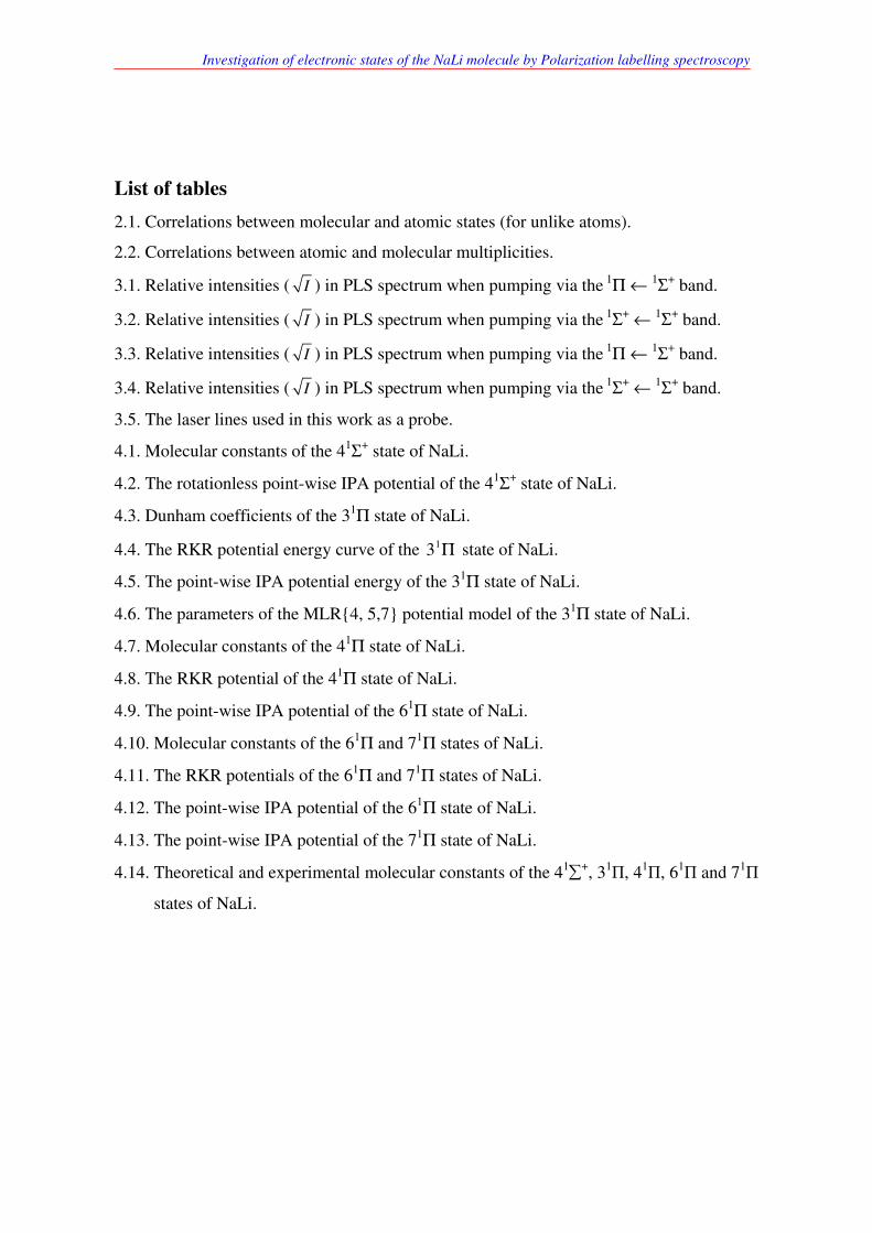
List of tables
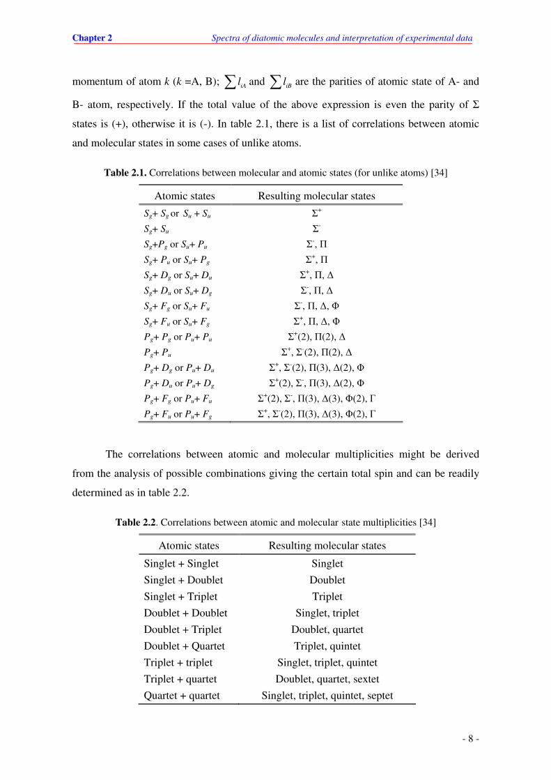
2.1. Correlations between molecular and atomic states (for unlike atoms).
2.2. Correlations between atomic and molecular multiplicities.
3.1. Relative intensities ( I ) in PLS spectrum when pumping via the 1Π ← 1Σ+ band.
3.2. Relative intensities ( I ) in PLS spectrum when pumping via the 1Σ+ ← 1Σ+ band.
3.3. Relative intensities ( I ) in PLS spectrum when pumping via the 1Π ← 1Σ+ band.
3.4. Relative intensities ( I ) in PLS spectrum when pumping via the 1Σ+ ← 1Σ+ band.
3.5. The laser lines used in this work as a probe.
4.1. Molecular constants of the 41Σ+ state of NaLi.
4.2. The rotationless point-wise IPA potential of the 41Σ+ state of NaLi.
4.3. Dunham coefficients of the 31Π state of NaLi.
4.4. The RKR potential energy curve of the 13 Π state of NaLi.
4.5. The point-wise IPA potential energy of the 31Π state of NaLi.
4.6. The parameters of the MLR4, 5,7 potential model of the 31Π state of NaLi.
4.7. Molecular constants of the 41Π state of NaLi.
4.8. The RKR potential of the 41Π state of NaLi.
4.9. The point-wise IPA potential of the 61Π state of NaLi.
4.10. Molecular constants of the 61Π and 71Π states of NaLi.
4.11. The RKR potentials of the 61Π and 71Π states of NaLi.
4.12. The point-wise IPA potential of the 61Π state of NaLi.
4.13. The point-wise IPA potential of the 71Π state of NaLi.
4.14. Theoretical and experimental molecular constants of the 41∑+, 31Π, 41
Π, 61Π and 71
Π
states of NaLi.

Investigation of electronic states of the NaLi molecule by Polarization labelling spectroscopy
List of figures
2.1. Coupling diagram of the angular momenta in Hund’s case (a).
2.2. The PEC of the 11Σ+ state of the NaLi molecule calculated theoretically [24]. The
equilibrium distance is Re = 2.89 Å, and the dissociation energy De = 7057cm-1.
2.3. Schematic outline of the algorithm for the IPA and DPotFit techniques.
2.4. Illustration of parity of rotational levels in the 1Σ+, 1Σ-, and 1Π states.
2.5. Potential energy diagrams with vertical transitions (Franck–Condon principle).
3.1. Scheme of the PLS method: P1 and P2 are the pair of crossed polarizers, D is detector
employed to detect polarization signal of the probe beam.
3.2. MJ - dependence of absorption cross-section (blue curves) for transitions between
Zeeman sublevels.
3.3. Excitation schemes in polarization labelling spectroscopy.
3.4. The three-section heat-pipe oven.
3.5. Experimental arrangement when the LD 500 dye laser system is used.
3.6. Experimental arrangement when the Frequency doubler-OPO/OPA system is used.
4.1. The PECs of the 1-71Π and 1-101
Σ+ states of NaLi calculated by Mabrouk et al [79].
The blue curves stand for 1Σ+ states, and the red ones stand for 1Π states.
4.2. A part of the PLS spectrum that consists of P and R lines when pump beam is
circularly polarized and probe at 15486.1 cm-1 excites simultaneously three transitions
starting at levels (0,30), (1,21) and (1,40) in the ground state. The vibrational quantum
numbers are denoted in figure.
4.3. Distribution of the experimental data in the field of quantum numbers of the 41Σ+ state
in NaLi.
4.4. Upper part: the solid curve represents the theoretical PEC for the 41Σ
+ state calculated
in [24], the solid-circle represents the IPA potential curve covered by experimental
data, and the circles represent the extrapolation of the IPA potential. Bottom: the dot-
star represents difference in energy between the current IPA potential and the
previous one [18].
4.5. A part of the PLS spectrum of the 31Π ←11Σ+ transitions observed in cases of linearly
(upper) and circularly (lower) polarized pumping light. In both cases the probe line is
set at 496.5 nm, thus labels level (0, 30) of the ground state.

Investigation of electronic states of the NaLi molecule by Polarization labelling spectroscopy
4.6. The envelope function (dashed) of the square of the FCFs (grey bar) and intensity
distribution of the observed spectral lines when labelling at level (1, 25).
4.7. Distribution of the experimental data in the field of quantum numbers of the 31Π state
in NaLi.
4.8. Plot R6[De-UMLR(R)] versus 1/R2 for different combinations of p, NS, NL parameters
in the MLR potential function.
4.9. Upper: the analytical MLR4, 5, 7 potential of the 31Π state of NaLi. Lower: the
curve of difference in energy between the IPA and MLR4, 5, 7 potentials.
4.10. Lambda-doubling strength function of the 31Π state of NaLi.
4.11. A part of PLS spectrum consists of P-, Q-, and R-lines of the 41Π ←11Σ+ band in
NaLi, observed in case of linearly polarized pump beam and 496.5 nm probe laser
line.
4.12. Distribution of the experimental data in the field of quantum numbers of the 41Π state
in NaLi.
4.13. The IPA potential of the 41Π state of NaLi, the red-solid circles stand for region
covered by experimental data, and the blue circles stand for extrapolation region.
4.14. Parts of PLS spectrum of the 61Π←11Σ band (red) and 71Π←11Σ (blue) observed in
the case of linearly polarized pump beam and 15539.3 cm-1 probe laser line. The
labelled level in this case is v"= 0 and J"= 22 in the ground state. Vibrational quantum
numbers of the progressions are indicated in figure.
4.15. Distribution of the experimental data in the field of quantum numbers of the 61Π state
in NaLi.
4.16. Distribution of the experimental data in the field of quantum numbers of the 71Π state
in NaLi.
4.17. The IPA potential curves of the 61П and 71
П states of NaLi
4.18. The potential energy curves of the 41Σ+ and 3-71Π states of NaLi calculated [79] (the
solid curves) and in our work (the solid-circles). The 51Π state has not been observed
in our experiment.
4.19. The theoretical potential energy curves of the 41Σ+ and 3-71Π states from [80] (the
solid curves) and the experimental ones (the solid-circles).
4.20. The theoretical potential curves of the 5-71Π states in [79] and [80], and the IPA
potential curves of the 61Π and 71
Π states determined in this work.

Investigation of electronic states of the NaLi molecule by Polarization labelling spectroscopy
Contents
Page
Abstract
List of tables
List of figures
1. Introduction 1
2. Spectra of diatomic molecules and interpretation of experimental data ......….. 5
2.1. Angular momenta and classification of electronic states ….......……………...…. 5
2.2. Correlations between atomic and molecular states …........………………….....…. 7
2.3. Schrödinger equation within the Born-Oppenheimer approximation …............ 9
2.4. Molecular constants and models of the potential ...................................….............. 12
2.4.1 Molecular constants …................……………………………………………………. 12
2.4.2 Dunham expansion…................……………………………….……………………... 15
2.4.3 Morse and Hulbert-Hirschfelder potentials ….........………………………… 17
2.4.4 RKR potential .………..………………………………………………..................……. 18
2.4.5 Long-range behaviour of potential energy curves ..........……….………… 19
2.4.6 Inverse perturbation approach and direct potential fit ….....……………. 21
2.5. Selection rules for optical transitions ...............................................................…..….. 23
2.5.1 Total parity and general selection rules...............…….……………..……….. 23
2.5.2 Selection rules …..................………………………………………………………….. 25
2.5.3 Franck-Condon principle ..............................................................................… 26
2.6. Perturbations in molecular spectra................................................................................. 27
2.6.1 Electrostatic and non-adiabatic perturbations ….......……………………... 27
2.6.2 Spin-orbit coupling …..............................…………………………………..... 29
2.6.3 Rotational perturbations …..............…………………….…………………………. 30

Investigation of electronic states of the NaLi molecule by Polarization labelling spectroscopy
3. Polarization labelling spectroscopy and experimental arrangement................. 33
3.1. Polarization labelling spectroscopy ….........…......….……………………................. 33
3.1.1 Basic principles …...................……………………………………………………….. 33
3.1.2 Amplitude of polarization signal ….............…………………………………….. 35
3.1.3 Excitation schemes …................................................…………………………….. 38
3.1.4 Relative intensities of spectral lines .............…………………………………... 39
3.2. Experimental……………..………………………………...………………...................…. 42
3.2.1 Preparation of NaLi molecules ……….............…………………………………. 42
3.2.2 Laser sources ………………………………………………………..................………. 44
3.2.3 Experimental arrangement ……..…………………………………….............…… 45
3.3. Determination of the absolute wavelength in PLS spectrum ............................... 47
4. Experimental results for the NaLi molecule ..……………………...........…………….. 48
4.1. Introduction …………………………………………………………....................………. 48
4.1.1 Historical overview of investigations of NaLi .......................................... 48
4.1.2 Outline of the electronic states observed in this work............................. 51
4.2. Methods of data analysis….………….................................…………………………………. 52
4.3. The 41Σ+ state ………………………….................................………………………………….. 53
4.3.1 Observation and assignment of the spectra …....................………………… 53
4.3.2 Molecular constants ……………………………………………..........................….. 55
4.3.3 Potential energy curve ……....................…………………………........................ 56
4.4. The 3 1Π state ………………………………..………………………….......................…. 59
4.4.1 Observation and assignment of the spectra ……….…………………........... 59
4.4.2 Dunham coefficients ……......…………………………………………................….. 62
4.4.3 Potential energy curve ……....................…………………………........................ 63
4.5. The 4 1Π state ......................……………………………………………………………… 71
4.5.1 Observation and assignment of the spectra …..........………………………... 71
4.5.2 Dunham coefficients ........................................................................................... 72
4.5.3 Potential energy curve ……....................…………………………........................ 73
4.6. The 51Π and 61Π states …………………….………………………….......................… 76

Investigation of electronic states of the NaLi molecule by Polarization labelling spectroscopy
4.6.1 Observation and assignment of the spectra ….....…….....………………….. 76
4.6.2 Dunham coefficients ............................................................................ 78
4.6.3 Potential energy curves …....................…………………………........................ 79
4.7 Comparison of the current results with recent theoretical calculations........... 83
5. Summary and conclusions .................…….……………………………………………….. 87
Bibliography............................................................................................................................................ 91

Chapter 1 Introduction
- 1 -
Chapter 1
Introduction
The alkali-metal diatomic molecules (dimers) have been for a long time very
attractive both for the theoreticians and experimentalists because they have a relatively
simple electronic structure. Their electronic structure is frequently considered by
theoreticians as a very convenient model for introducing and testing of several
approximations which can be further applied to more complex molecular systems. But the
final verification of applied theoretical assumptions and approximations is always provided
by experiment. From the experimental point of view alkali-metal dimers with their main
absorption bands placed in the visible and UV regions are very convenient objects for
investigations with modern laser spectroscopy techniques. Investigations of alkali-metal
dimers have recently experienced additional impetus since Bose-Einstein condensate in
dilute alkali-metal vapors was obtained [1] and presently there are many efforts to create
ultra-cold molecules and molecular condensates consisting of different alkali-metal
mixtures [2-8]. This makes the precision data delivered by spectroscopists crucial for
planning and interpretation of this new class of experiments. The heteronuclear cold
molecules are considered to be particularly interesting because they possess a permanent
dipole moment and can therefore interact (be manipulated) with external electric fields.
Among alkali-metal dimers, the knowledge of the electronic structure of
heteronuclear molecules is less advanced than for homonuclear ones. In particular for
NaLi, the lightest and simplest heteronuclear alkali-metal dimer, the number of
investigated electronic states is quite modest. The first experimental observation of the
spectrum of this molecule was reported only in 1971 by Hessel [11] while other dimers
were observed experimentally as early as 1928 [9]. Up to now, only few singlet-electronic
states have been studied experimentally [12-18]. On the theoretical side, the pioneering
study of the NaLi molecule was performed by Bertocini et al [19] in 1970. After that
Chapter 1 Introduction
- 2 -
several research groups used ab initio techniques to explore the electronic structure of this
molecule [20-24]; the most systematic and accurate were carried out by Schmidt-Mink et
al [24] and concerned the first sixteen singlet and triplet states of NaLi. Relatively poor
knowledge of the electronic structure of the NaLi molecule when compared with those for
the other dimers was one of the motivations of the present study. But it is also worth
mentioning at this point that Li and Na atoms have been already simultaneously trapped
and cooled in a magneto-optical trap (MOT) [4-6] which gives good prospects for further
work on cold NaLi in the near future.
Growing interest in the NaLi molecule resulted very recently (June and August
2008) in two new theoretical papers [79, 80] by two independent research teams. For the
first time the authors give comprehensive descriptions of highly excited states, particularly
of those that were for the first time investigated experimentally in the present study. Since
theoretical results presented in both papers differ considerably this makes comparison with
our results particularly relevant, and therefore we anticipate that the existing discrepancy
between the two theoretical predictions will be explained by theoreticians.
In fact we carried out our experiments much earlier, before the theoretical
calculations were made and we were able to interpret and assign the observed spectral lines
to individual electronic states on the basis of results of our experiments, analysed by
numerical algorithms developed in our laboratory. Presently, when we have two theoretical
sources for comparison we are able to critically evaluate them.
In order to attempt experimental investigations of the NaLi molecule one has to
find a way to form a sufficiently dense sample of the molecules and then to selectively
observe the spectra originating from the NaLi molecule, even though they coexist with the
Na2 and Li2 ones. The main problem in production of NaLi molecules comes from a big
difference of melting temperatures of metallic sodium and lithium resulting in big
difference of Na and Li densities in the gas phase. In the present experiment we overcame
this difficulty by using a special design of a heat-pipe oven, similar to the construction
already proved in investigations of KLi molecules [32]. Furthermore, selective
observations of NaLi spectra were carried out by means of polarization labelling
spectroscopy (PLS). Originally this method was invented by Schawlow and Hänsch [27]
and with some modifications [28] has been used in Warsaw for investigations of Li2 [29],
Na2 [30], K2 [31], NaK [31], KLi [32] and NaRb [33]. The method depends on the use of
two lasers: one selectively labels molecular levels while the other one induces optical

Chapter 1 Introduction
- 3 -
transitions from labelled levels to the investigated electronic state. By proper choice of the
wavelength of the labelling laser we could strongly suppress unwanted spectra of
homonuclear molecules thus making the analysis feasible. The experiment was performed
using the polarization labeling spectroscopy technique, in a version based on the V-type
optical - optical double resonance scheme.
The analysis of raw data and finally the description of the electronic states were
performed by several methods with computer codes already developed in our laboratory.
First of all we identified in the recorded spectra spectral lines corresponding to the
investigated states and assigned quantum numbers of levels involved in each transition. For
all states molecular constants (Dunham coefficients) were determined. Potential energy
curves were then constructed numerically by different methods: semiclassical one (RKR,
based WKB approximation), by fully quantum inverted perturbation approach technique
[54, 55] (IPA, point-wise implementation [57]) and in the case of one state with the direct-
potential-fit technique (DPotFit, with codes from [58]). The most reliable and accurate
potential energy curves capable of reproducing experimental data within the demanded
accuracy were obtained with the IPA technique and together with the molecular constants
were the subject of comparison with the theoretical results.
In this thesis the results of experimental investigation by means of the PLS
technique on the 41Σ
+, 31Π, 41
Π, 61Π, and 71
Π states of NaLi are described. All 1Π-symetry
states mentioned above were observed for the first time. Some of these results were already
published in the following papers:
1. Nguyen Huy Bang, W. Jastrzębski, and P. Kowalczyk. New observation and
analysis of the E(4)1Σ+ state in NaLi. J. Mol. Spectr. 233 (2005) 290-292.
2. Nguyen Huy Bang, A. Grochola, W. Jastrzębski, P. Kowalczyk, and H. Salami.
Investigation of a highly excited electronic 1Π state of NaLi molecule. Optica
Applicata 36 No4 (2006) 499-504.
3. Nguyen Huy Bang, A. Grochola, W. Jastrzębski, and P. Kowalczyk. First
observation of 31Π and 41Π states of NaLi molecule. Chem. Phys. Lett, 440
(2007) 199-202.
4. Nguyen Huy Bang, A. Grochola, W. Jastrzębski, and P. Kowalczyk. Spectroscopy
of mixed alkali dimers by polarization labelling technique: application to NaLi and
NaRb molecules. Opt. Mat. (2008) in press.
Chapter 1 Introduction
- 4 -
This thesis is organized in the following way:
• Chapter 2 is devoted to presentation of the basic information about the electronic
structure of diatomic molecules, standard approximations made in descriptions of
electronic states, selection rules for optical transitions and different techniques of
processing and interpretation of experimental data (i.e. molecular constants and
potential energy curves). Additionally some information about the origin of
perturbations of molecular levels is presented.
• Chapter 3 discusses the basic concepts of polarization labelling spectroscopy,
presents comparison of different schemes which can be used in experiments and of
relative intensities of spectral lines (polarization signal) observed for different
arrangements of polarization and different symmetry of states involved in labelling
process. Also a short description of the main parts of the experimental set-up is
given together with the procedure for precise frequency calibration of the spectra.
• Chapter 4 collects results obtained for the 41Σ
+, 31Π, 41
Π, 61Π, and 71
Π states of
NaLi with first comparison with theoretical predictions for these states. For each of
the investigated states molecular (Dunham) constants and potential energy curves
calculated with different methods are presented.
• Chapter 5 includes conclusions, and discussion of discrepancies between
experimental and theoretical results in a review of the most recent calculations.
• Finally there is a bibliography concerning literature presented in this thesis.
Chapter 2 Spectra of diatomic molecules and interpretation of experimental data
- 5 -
Chapter 2
Spectra of diatomic molecules and interpretation of experimental data
2.1. Angular momenta and classification of electronic states
Consider a diatomic molecule that consists of two nuclei A and B surrounded by
fast-moving electrons. If we disregard nuclear spin, which is responsible for the hyperfine
structure, then there are three sources of angular momentum in a diatomic molecule: the
spin of the electrons S
, the angular momenta due to orbital motion of electrons L , and the
rotation of the molecular framework R . The nuclear charges produce an axial symmetric
electric field about the internuclear axis. In such field the resultant electronic angular
momentum L precesses very fast about the axis. Hence, only the component ML of
L
along the internuclear axis is well defined. On the other hand, if one reverses the sense of
moving direction of all electrons the sign of ML is changed to – ML but the energy of
system will not be changed. Thus the states that differ only by the sign of ML have the
same energy (two-fold degeneracy) whereas the states with different values of |ML| have in
general different energies. Therefore it is convenient to classify the electronic states of
diatomic molecules according to:
Λ = |ML|, Λ = 0, 1, 2 … (in ħ unit) (2.1)
According to Λ = 0, 1, 2, 3 … the corresponding electronic states are denoted as Σ,
Π, ∆, Φ, .. . Among those, the Π, ∆, Φ, … states are doubly degenerated since ML can have
two +Λ and -Λ values, whereas the Σ states are non-degenerated.
In a diatomic molecule symmetric properties of electronic wavefunctions depend
on the symmetry of the electric field in which the electrons move. Any plane through the
internuclear axis is the plane of symmetry. Namely, the electronic wavefunctions either do
not change or change their sign to opposite under a reflection of electronic coordinates in
respect to the plane of symmetry. The first kind of states are classified as (+) parity
Chapter 2 Spectra of diatomic molecules and interpretation of experimental data
- 6 -
whereas the last one as (-) parity. The parity symbol (+/-) is placed as right superscript for
the notation of electronic state. In addition to the plane of symmetry, homonuclear
diatomic molecules also have a centre of symmetry (middle point of internuclear distance)
which leaves the electric field unaltered under reflection of coordinates of the nuclei
against this point. Upon such reflection the electronic wavefunctions either do not change
or change their sign. The states belong to the first type are called gerade (labelled by right
subscript g), and the states belong to the second type are called ungerade (right subscript
u).
Whenever spin of electrons is taken in to account, the spin of individual electrons
can form a resultant spin moment S with the corresponding quantum number S. Since
upon the orbital motion of electrons a magnetic field is produced along internuclear axis,
this causes a precession of S about the axis with a component along axis denoted by Σ.
For a given value of S there are 2S+1 possible values of Σ which correspond to different
energies for a given value of Λ. The value of 2S+1 called the multiplicity of the electronic
state is marked as left superscript in the notation of electronic state, 2S+1Λ. In addition to the
Λ and Σ quantum numbers in some notations also quantum number Ω is used and defined
as follows:
Ω = | Λ + Σ |. (2.2)
In spectroscopic nomenclature there are two ways to number electronic states: The
first one is to label electronic states by letters in which X is for the ground state, while A, B,
C, … label successively excited states of the same multiplicity as the ground state. States
with multiplicity different from that of the ground state are labelled with lowercase letters
a, b, c, … . An alternative way, becoming currently a standard one, is to label states of the
same symmetry by integers: 1 for the state of lowest energy state of each multiplicity, and
2, 3, … for the successive excited states (in each multiplicity-class).
The angular momenta described above are referred to fixed- molecular frame. Since
the rotation of the molecule leads to a rotation of nuclear framework a rotational angular
momentum R perpendicular to the internuclear axis is formed. Therefore,
ΩΩΩΩ couples with
R (fig. 2.1) resulting in a total angular momentum
J determined by:
= + = + + J R RΩ Λ ΣΩ Λ ΣΩ Λ ΣΩ Λ Σ . (2.3)

Chapter 2 Spectra of diatomic molecules and interpretation of experimental data
- 7 -
Such coupling scheme of angular momentums is known as Hund’s case (a) [34]
and it is a good approximation for many electronic states of diatomic molecules. Following
this scheme the total angular momentum is quantized in a fixed free-space with the
quantum number J. It is worth to point out that within the framework of Hund’s case (a),
the J, S, Ω, Λ, Σ is a good set of quantum numbers to represent quantum states of
rotating molecule. In addition to the Hund's case (a) coupling scheme there are also other
coupling schemes which are called Hund's case (b), (c), and (d) [34].
2. 2. Correlations between atomic and molecular states
In diatomic molecules correlations between atomic and molecular states might be
derived within the separated-atom model [34]. Following assumptions of this model,
couplings between angular momenta in the constituent atoms are assumed to obey the
Russell-Saunders scheme, where atomic states are determined in the central field
approximation [36]. By adding the components (along the internuclear axis) of the total
angular momenta of individual atoms one can obtain several possible values of Λ giving
rise to different molecular electronic states. The parity in particular case of Σ-symmetry
states is determined according to parity of electronic atomic states and total angular
momentum of atoms, following Wigner and Witmer correlation rules [34]. Namely, the
parity of the Σ states depends on A B iA iBL L l l+ + +∑ ∑ , where Lk is total angular
Figure 2.1. Coupling diagram of the angular momenta in Hund’s case (a).
A B
J
R
L
S
ΛΛΛΛ
ΣΣΣΣ
ΩΩΩΩ
Chapter 2 Spectra of diatomic molecules and interpretation of experimental data
- 8 -
momentum of atom k (k =A, B); iA
l∑ and iB
l∑ are the parities of atomic state of A- and
B- atom, respectively. If the total value of the above expression is even the parity of Σ
states is (+), otherwise it is (-). In table 2.1, there is a list of correlations between atomic
and molecular states in some cases of unlike atoms.
Table 2.1. Correlations between molecular and atomic states (for unlike atoms) [34]
Atomic states Resulting molecular states
Sg+ Sg or Su + Su Σ+
Sg+ Su Σ-
Sg+Pg or Su+ Pu Σ-, Π
Sg+ Pu or Su+ Pg Σ+, Π
Sg+ Dg or Su+ Du Σ+, Π, ∆
Sg+ Du or Su+ Dg Σ-, Π, ∆
Sg+ Fg or Su+ Fu Σ-, Π, ∆, Φ
Sg+ Fu or Su+ Fg Σ+, Π, ∆, Φ
Pg+ Pg or Pu+ Pu Σ+(2), Π(2), ∆
Pg+ Pu Σ+, Σ-(2), Π(2), ∆
Pg+ Dg or Pu+ Du Σ+, Σ-(2), Π(3), ∆(2), Φ
Pg+ Du or Pu+ Dg Σ+(2), Σ-, Π(3), ∆(2), Φ
Pg+ Fg or Pu+ Fu Σ+(2), Σ-, Π(3), ∆(3), Φ(2), Γ
Pg+ Fu or Pu+ Fg Σ+, Σ-(2), Π(3), ∆(3), Φ(2), Γ
The correlations between atomic and molecular multiplicities might be derived
from the analysis of possible combinations giving the certain total spin and can be readily
determined as in table 2.2.
Table 2.2. Correlations between atomic and molecular state multiplicities [34]
Atomic states Resulting molecular states
Singlet + Singlet Singlet
Singlet + Doublet Doublet
Singlet + Triplet Triplet
Doublet + Doublet Singlet, triplet
Doublet + Triplet Doublet, quartet
Doublet + Quartet Triplet, quintet
Triplet + triplet Singlet, triplet, quintet
Triplet + quartet Doublet, quartet, sextet
Quartet + quartet Singlet, triplet, quintet, septet

Chapter 2 Spectra of diatomic molecules and interpretation of experimental data
- 9 -
2.3. Schrödinger equation within the Born-Oppenheimer approximation
Consider a molecule consisting of n electrons and two nuclei, A and B. In a
laboratory frame the non-relativistic Schrödinger equation of the system can be written as
ˆ EΨ = ΨH . (2.4)
Here, Ψ - total wavefunction, H -the total Hamiltonian operator which consists of kinetic
energy operator of nuclei ( ˆ NT ), interaction potential between the two nuclei ( NNV ) and the
Hamiltonian of electrons ( ˆ elH ). In details the total Hamiltonian is written by:
ˆ ˆ ˆ= + +N NN elH T V H , (2.5)
2 22
ˆ2
A B
A BM M
∇ ∇= − +
NT
, (2.6)
2
A BZ Z e
R=NN
V , (2.7)
2 22 2
2
1 1 1
ˆ2
n n nA B
i
i i i je Ai Bi ij
Z e Z e e
m r r r= = < =
= − ∇ − + +
∑ ∑ ∑el
H
. (2.8)
In the above expressions, i stands for the ith electron, R is the internuclear distance, rij is
relative distance between ith electron and jth particle (electron or nucleus), M and me are
respectively masses of nucleus and electron; ZA and ZB are atomic numbers of the nuclei A
and B, respectively.
In order to solve Eq. (2.4) Born and Oppenheimer proposed an approximation (so
called Born-Oppenheimer approximation, abbreviated by BO) in which the motion of
electrons and nuclei can be treated separately in two steps. In the first step it is recognized
that the nuclei as much heavier than the electrons ( emM
< 1/1800) move very slowly in
comparison to the electronic motion. Thus the kinetic energy operator of nuclei can be
neglected when considering ˆ elH . Therefore the total wavefunction can be factorised as
product of the nuclear and electronic parts:
( ) ( , )tot BOR r RψΨ ≈ Ψ = Φ
. (2.9)
Chapter 2 Spectra of diatomic molecules and interpretation of experimental data
- 10 -
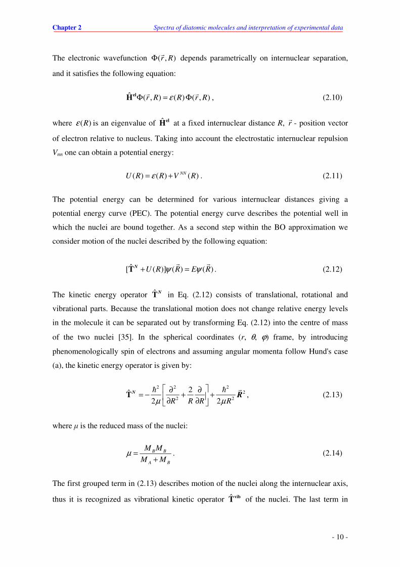
The electronic wavefunction ( , )r RΦ
depends parametrically on internuclear separation,
and it satisfies the following equation:
ˆ ( , ) ( ) ( , )r R R r RεΦ = ΦelH
, (2.10)
where ( )Rε is an eigenvalue of ˆ elH at a fixed internuclear distance R, r
- position vector
of electron relative to nucleus. Taking into account the electrostatic internuclear repulsion
Vnn one can obtain a potential energy:
( ) ( ) ( )NNU R R V Rε= + . (2.11)
The potential energy can be determined for various internuclear distances giving a
potential energy curve (PEC). The potential energy curve describes the potential well in
which the nuclei are bound together. As a second step within the BO approximation we
consider motion of the nuclei described by the following equation:
ˆ[ ( )] ( ) ( )U R R E Rψ ψ+ =T
N . (2.12)
The kinetic energy operator TN in Eq. (2.12) consists of translational, rotational and
vibrational parts. Because the translational motion does not change relative energy levels
in the molecule it can be separated out by transforming Eq. (2.12) into the centre of mass
of the two nuclei [35]. In the spherical coordinates (r, θ, ϕ) frame, by introducing
phenomenologically spin of electrons and assuming angular momenta follow Hund's case
(a), the kinetic energy operator is given by:
2 2 2
22 2
2ˆ2 2R R R Rµ µ
∂ ∂= − + +
∂ ∂ T
N R , (2.13)
where µ is the reduced mass of the nuclei:
B B
A B
M M
M Mµ =
+. (2.14)
The first grouped term in (2.13) describes motion of the nuclei along the internuclear axis,
thus it is recognized as vibrational kinetic operator ˆ vibT of the nuclei. The last term in

Chapter 2 Spectra of diatomic molecules and interpretation of experimental data
- 11 -
(2.13) depends on the rotational angular momentum R and it is recognized as rotational
kinetic operator ˆ rotT . Since the rotational and vibrational motions are separable the
wavefunction ( , , )rψ θ ϕ of the nuclei can therefore be factorized as the product of the
vibrational and rotational parts:
1
( , , ) ( ) ( , ) ( ) ( , )vib rot rotR R u R u
Rψ θ ϕ ξ θ ϕ χ θ ϕ= = . (2.15)
The operator ˆ rotT acts on the wavefunction ( , )rotu θ ϕ giving rotational energy given by:
2 2[ ( 1) ( 1) ]rotE B J J S S= + − Ω + + − Σ , (2.16)
where
2
22B
Rµ=
. (2.17)
Substituting (2.15) and (2.13) into (2.12) and regarding (2.16), we obtain:
2 2
2 2( ) ( ) ( )
2rot
q q q
dE U R R E R
R dRχ χ
µ
−+ + =
, (2.18)
where, q stands for all quantum numbers representing the state of the molecule. The
expression (2.18) is known as the Radial Schrödinger Equation (RSE) and describes
rovibrational motion of the nuclei under an effective potential energy, Ueff(R):
( ) ( ) rot
effU R U R E= + . (2.19)
For the singlet states (Σ = 0, Ω = Λ) the RSE is reduced to:
2 2
22
[ ( 1) ] ( ) ( ) ( )2 q q q
dB J J U R R E R
dRχ χ
µ
−+ + − Λ + =
. (2.20)
It is worth to remark here that within the framework of the BO approximation the
Schrödinger equation of a diatomic molecule is greatly simplified to the RSE from the Eq.
(2.18). From the theoretical point of view, in order to calculate U(R) one needs to have a
model that is capable to represent adequately interactions in the molecule (see [38], for
example). The theoretical methods for calculations of potential energy curve are presented

Chapter 2 Spectra of diatomic molecules and interpretation of experimental data
- 12 -
Figure 2.2. The PEC of the 11Σ+ state of the NaLi molecule calculated theoretically [24]. The
equilibrium distance is Re = 2.89 Å, and the dissociation energy De = 7057 cm-1.
in many textbooks and are beyond the scope of this thesis. From the experimental point of
view, the determination of U(R) is carried out in a different way. Namely, from the
experimentally observed spectral lines one can determine the energy levels of the
molecule. Having energy levels it is possible to determine the potential energy curve of the
molecule (see sect.2.4). Therefore such experimental potential curve besides giving
spectroscopic characterization of the molecular state, also gives the way to compare
experimental PEC with obtained theoretically.
In practice, the RSE (2.18) is well applicable to represent experimental level
energies of heavy molecules. However, for light molecules like hydrides the RSE is often
inadequate to describe experimental data because in these molecules the assumption for
neglecting the kinetic energy of the nuclei when describing electrons motion is no longer
valid. Therefore, in this case higher-order corrections must be taken in to account. These
corrections will be presented in section 2.6.
2.4. Molecular constants and models of the potential
2.4.1 Molecular constants
In case of bound electronic states the PEC has the following common properties [34, 39-
40] (fig. 2.2):

Chapter 2 Spectra of diatomic molecules and interpretation of experimental data
- 13 -
• It has a minimum at an equilibrium internuclear distance, denoted as Re.
• It should approach asymptotically to a finite value as R goes to infinity. The
energy which is needed to separate the atoms forming the molecule from the
equilibrium distance to infinity is called dissociation energy, denoted by De.
• Around the equilibrium, the potential function behaves approximately as the
harmonic one.
• It should become infinite at R = 0. This is merely a pure mathematic
condition. The repulsive electrostatic force between the nuclei increases
rapidly when nuclei approach each other from the equilibrium internuclear
distance.
Following those properties, one can derive an expression of level energies. The potential
energy function U(R) can be expanded in Taylor's series around the equilibrium
internuclear distance:
(1) (2) 21( ) ( ) ( )( ) ( )( )
2!e e e e eU R U R U R R R U R R R= + − + −
(3) 3 (4) 41 1( )( ) ( )( ) ...,
3! 4!e e e eU R R R U R R R+ − + − + (2.21)
where:
( ) ( )( ) , 1, 2,...
e
mm
e m
R R
d U RU R m
dR=
= =
In (2.21), the second term vanishes due to the minimum at Re, the third term corresponds to
harmonic potential with a force constant k = U(2)(Re). By introducing a new variable y =
R - Re the expression (2.21) has a form as:
2 (3) 2 (4) 41 1 12 6 24( ) (0) (0) (0) ...U q U ky U y U y= + + + + (2.22)
The RSE (2.20) now becomes:
2 2 2
22 2
1[ ( 1) ] ( ) ( ) ( )
2 2 ( ) q q q
e
dJ J U y y E y
dy R yχ χ
µ µ
−+ + − Λ + =
+
. (2.23)
Around the equilibrium distance we can expand:

Chapter 2 Spectra of diatomic molecules and interpretation of experimental data
- 14 -
2
22 2
2
1 1 1 2 31 ...
( )1
e e e e
e
e
y y
R y R R RyR
R
= = − + −
+ +
. (2.24)
In the zero-order approximation we retain the first two terms in (2.22) and the first
term in (2.24) and then substituting them into (2.23) we obtain the so called spectroscopic
term as follows:
, 212( , ) ( ) [ ( 1) ]v J
e e e
ET v J T v B J J
hcω= = + + + + − Λ , (2.25)
where
1
/2e k
cω µ
π=
, (2.26)
24e
e
Bc Rπ µ
=
. (2.27)
The first term on the right-hand side of (2.25) is called electronic energy which
corresponds to the value of potential energy at the equilibrium internuclear distance. The
second term represents energy of harmonic oscillator with a vibrational constant ωe which
relates to strength of chemical bonding between the two atoms. The last term is the energy
due to the rotation of the molecule. It is described by a rotational constant Be relating to
bond length.
In the first-order approximation the expanded potential is retained up to y4 whereas
expression (2.24) is retained up to y2. Using perturbation theory, we obtain:
2 21 12 2( , ) ( ) ( ) [ ( 1) ]e e e e eT v J T v x v B J Jω ω= + + − + + + − Λ -
2 2 2 212[ ( 1) ] ( )[ ( 1) ]
e eD J J v J Jα− + − Λ − + + − Λ . (2.28)
The third term in (2.28) represents a contribution to the unharmonicity of the potential. In
most cases ωexe > 0 and ωexe << ωe, thus vibrational spacing decreases gradually as one
approaches to higher vibrational levels. The fifth term in (2.28) is responsible for
centrifugal effect due to the rotation of molecule. The last term in (2.28) represents
coupling between rotations and vibrations.
In general, higher approximations can be carried out to obtain the higher corrections for the
spectroscopic term. Following these, the spectroscopic term is given by [34]:

Chapter 2 Spectra of diatomic molecules and interpretation of experimental data
- 15 -
T (v, J) = Te + G (v) + Fv (J), (2.29)
where
G (v) = ωe (v+ 12 ) - ωexe (v+ 1
2 ) 2 + ωeye(v+ 12 ) 3 +... (2.30)
Fv(J) = Bv J(J+1) – Dv [J(J+1)]2 + Hv [J(J+1)]3 +..., (2.31)
Bv = Be - αe (v+ 12 ) +...,
24e
e
Bc Rµ
=
(2.32)
Dv = De - βe (v+ 12 ) +...,
3
2
4 ee
e
BD
ω= (2.33)
Hv = He +..., 2 2
2
3 (12 )e
e
e e e e
DH
Bω α ω=
−. (2.34)
2.4.2 Dunham expansion
An alternative, but more general, form than the molecular constants for
representation of level energies of a diatomic molecule was derived by Dunham [41]. In
this method the effective potential in (2.19) is expanded in terms of power series
2 21 2( ) (1 ...)
eff e oU T a a aξ ξ ξ ξ= + + + + +
2 2 3[ ( 1) ](1 2 3 4 ...)e
B J J ξ ξ ξ+ + − Λ − + − + , (2.35)
with
e
e
R R
Rξ
−= , (2.36)
and ai (i = 0, 1, 2…) are constants determined with derivatives of the Dunham potential.
The first term in (2.35) is electronic energy, the second grouped-term represents vibrational
potential of the nuclei, and the last grouped-term stands for the rotational energy of the
molecule.
Although the exact solution of the RSE is not possible to derive with the Dunham
potential but one can find it within the semiclassical approximation. Indeed, using the first-
order semiclassical quantization condition (Wentzel-Kramers-Brillouin (WKB) theory
[42]) Dunham solved the RSE with the potential (2.35) yielding expression for the
spectroscopic term as follows:

Chapter 2 Spectra of diatomic molecules and interpretation of experimental data
- 16 -
212( , ) ( ) [ ( 1) ]i k
e ik
i k
T v J T Y v J J= + + + − Λ∑∑ . (2.37)
In (2.37), Yjk (i = 0, 1, 2…; k = 0, 1, 2…) are Dunham coefficients which are related to the
expansion coefficients ai in (2.35). The relations between the Yik and ai coefficients can
be found in [41]. On the other hand, by comparing (2.37) with (2.29) we obtain the
following relations between the Dunham coefficients and molecular constants:
Y10 = ωe, Y20 = - ωexe, Y30 = ωeye
Y01 = Be Y11 = -αe Y21 = γe (2.38)
Y02 = - De Y12 = -βe Y03 = He.
Actually it was pointed out by Dunham that there are some small deviations
between Dunham coefficients and molecular constants in relations (2.38). These deviations
are of the order of 2 2 6/ ~ 10e eB ω − ; therefore they are negligible. There is also a small non-
zero term Y00:
2 2
00 44 12 144 4e e e e e e e
e e
B xY
B B
α ω α ω ω= + + − . (2.39)
Small value of Y00 is because the first three terms in (2.39) are almost cancelled by the last
one, and in most cases Y00 is incorporated into the electronic energy Te.
Since the molecular constants are nuclear mass-dependent the values of the
Dunham coefficients are therefore altered from one isotopomer to the other. Within the BO
approximation the vibrational potential energy curves of different isotopomers are
identical. Therefore for an isotope with a reduced-mass µα, the Dunham expansion should
be modified to [34]:
[ ]( ) 2 212( , ) ( ) [ ( 1) ]
ki
e ik
i k
T v J T Y v J Jα ρ ρ = + + + − Λ ∑∑ , (2.40)
where
α
µρ
µ= . (2.41)
The Dunham expansion is widely used to represent level energies of diatomic
molecules because such representation is quite simple and is able to represent the high
order effects such as unharmonicities of the potential, centrifugal forces, as well as

Chapter 2 Spectra of diatomic molecules and interpretation of experimental data
- 17 -
couplings between vibrational and rotational motions. However some drawbacks may be
encountered in application of the Dunham method. Indeed, as pointed out by Beckel [43],
the Dunham potential is convergent in the region for which R < 2Re. For low vibrational
levels the inner and outer turning points of the potential are around the equilibrium
internuclear distance, thus the Dunham expansion represents fairly well experimental data.
When experimental data lie closely the dissociation limit, the outer turning points of highly
vibrational levels exceed 2Re, the power series is thus gradually diverged. In this case more
coefficients, some of them of no physical meaning, are needed to describe the overall
experimental data.
2.4.3 Morse and Hulbert-Hirschfelder potentials
One of the important models of the analytical potential was proposed by Morse
[44] in the following form
22 ( ) /( ) 1 e eR R RMorse e
eU R T D eβ− − = + − . (2.42)
Where: Te, De, and Re stand for the electronic energy, dissociation energy, and the
internuclear equilibrium distance, respectively; β is a parameter. If one disregards the
rotation of molecule, the RSE with this potential can be solved analytically yielding the
vibrational energy. Comparing this analytical result to expression (2.30), we obtain
correspondence of β and De with the molecular constants:
ee
c
D
π µβ ω=
,
2
4e e
e e
Dx
ω
ω= . (2.43)
Additionally taking into account the rotational motion of molecule Pekeris [47] solved the
RSE with Morse potential by using perturbation techniques. He obtained an expression for
rotational energy of the form (2.31) and among some molecular constants:
12
3
2
43( / ) 3( / ) , e
e e e e e e e e e e
e
BB x B x B x Dα ω ω
ω = − =
. (2.44)
The first expression of (2.44) gives quantitative relation between the rotational and
vibrational motions of the molecule; the second expression represents a relation among the
Chapter 2 Spectra of diatomic molecules and interpretation of experimental data
- 18 -
centrifugal, rotational and vibrational constants. By replacing these molecular constants
with the corresponding Dunham coefficients we obtain the so called Kratzer relation [47]:
3
0102 2
10
( )4
( )
YY
Y= − . (2.45)
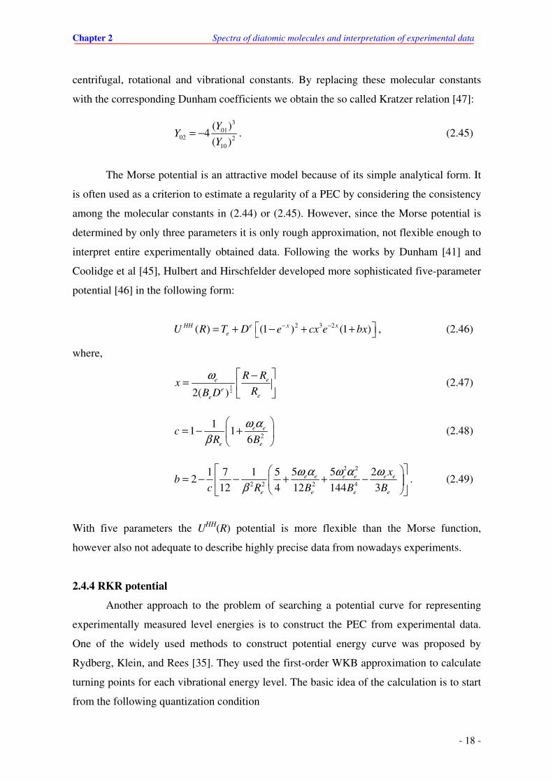
The Morse potential is an attractive model because of its simple analytical form. It
is often used as a criterion to estimate a regularity of a PEC by considering the consistency
among the molecular constants in (2.44) or (2.45). However, since the Morse potential is
determined by only three parameters it is only rough approximation, not flexible enough to
interpret entire experimentally obtained data. Following the works by Dunham [41] and
Coolidge et al [45], Hulbert and Hirschfelder developed more sophisticated five-parameter
potential [46] in the following form:
2 3 2( ) (1 ) (1 )HH e x x
eU R T D e cx e bx− − = + − + + , (2.46)
where,
122( )
e e
eee
R Rx
RB D
ω −=
(2.47)
2
11 1
6e e
e e
cR B
ω α
β
= − +
(2.48)
2 2
2 2 2 4
5 5 21 7 1 52
12 4 12 144 3e e e e e e
e e e e
xb
c R B B B
ω α ω α ω
β
= − − + + −
. (2.49)
With five parameters the UHH(R) potential is more flexible than the Morse function,
however also not adequate to describe highly precise data from nowadays experiments.
2.4.4 RKR potential
Another approach to the problem of searching a potential curve for representing
experimentally measured level energies is to construct the PEC from experimental data.
One of the widely used methods to construct potential energy curve was proposed by
Rydberg, Klein, and Rees [35]. They used the first-order WKB approximation to calculate
turning points for each vibrational energy level. The basic idea of the calculation is to start
from the following quantization condition

Chapter 2 Spectra of diatomic molecules and interpretation of experimental data
- 19 -
2
1
( )1/ 21
,2( )
2( ) [ ( )]
R v
v J J
R v
v E U R dRµ
π
+ = −
∫
. (2.50)
In (2.50), UJ(R) is the effective potential; R1 (v) and R2 (v) are inner and outer turning
points, respectively. The turning points are determined from:
Ev J = UJ (R1 (v)) = UJ (R2 (v)).
Next, the vibrational quantum number v is treated as a continuous function of energy. The
equation (2.50) can therefore be partially differentiated with respect to E and to J (J+1).
Finally one obtains two coupled equations for turning points:
2 '
1 2 ' 1/ 2( ) ( ) 22 [ ( ) ( )]
o
v
v
dvR v R v
G v G vµ− =
−∫
, (2.51a)
' '
2 ' 1/ 21 2
1 1 22
( ) ( ) [ ( ) ( )]o
v
v
v
Bdv
R v R v G v G v
µ− =
−∫
. (2.51b)
Here, vo is an extrapolated value of the vibrational quantum number to the potential
minimum, it is given by:
0012o
e
Yv
ω= − − . (2.52)
In practice, the functions Bv and G(v) can be determined from experimental data
therefore the RKR potential curve determined with pairs of turning points can be readily
numerically calculated.
2.4.5 Long-range behaviour of potential energy curves
Since depending on internuclear distance different forces (exchange or dispersion
forces) dominate, it is convenient to divide the potential into the short-range and long-
range parts in order to describe the PEC of a molecule. The short-range part involves
chemical bonding which depends strongly on the overlap of electronic clouds between the
two atoms and is governed by exchange forces. The long-range part involves the dispersion
forces which are resulting from electrostatic, induction, and resonance forces. It is usual to
represent the long-range part of a potential by the following form:
Chapter 2 Spectra of diatomic molecules and interpretation of experimental data
- 20 -
( ) e n
nn
CU R D
R= −∑ . (2.53)
From (2.53) one can see that the potential approaches the dissociation energy when the two
atoms are separated infinitively. The dispersion coefficients Cn are determined according to
the atomic electronic states at which the given molecule dissociates. From basic quantum -
mechanical considerations one can see that dominant terms in the expansion (2.53) depend
on symmetry of asymptotic atomic states. Namely [48]:
• For homonuclear diatomic molecules:
For nS – n'S asymptote, dominant terms in (2.53) are with n = 6, 8, 10…
nS – n'P asymptote: n = 3, 6, 8, 10 …
nS – n'D asymptote: n = 5, 6, 8, 10 …
nP – n'P asymptote: n = 5, 6, 8, 10 …
• For heteronuclear diatomic molecules:
nS – n'S asymptote: n = 6, 8, 10 …
nS – n'P asymptote: n = 6, 8, 10 …
nS – n'D asymptote: n = 6, 8, 10 …
nP – n'P asymptote: n = 5, 6, 8, 10 …
For alkali diatomic molecules, Marinescu et al [49-52] calculated coefficients Cn in
framework of the second-order perturbation theory.
We determine the pure long-range region as a range for which the exchange
interactions are weaker compared to the dispersion forces. LeRoy [48] proposed a
quantitative criterion for determining the value of internuclear distance from which the
expansion (2.53) is valid. Following his work the long-range expansion (2.53) is valid for
atomic separation larger than the so called LeRoy radius RLR, given by
1 12 22 22
LR A BR r r = +
. (2.54)
Here 122
r is the root mean square of radius of the outermost electron of the atom. Since
for non-spherical atomic orbitals the spatial distribution of the charge-cloud of the
outermost electron depends on spatial orientation of the overlap between outermost

Chapter 2 Spectra of diatomic molecules and interpretation of experimental data
- 21 -
electrons, thus depends on the projection of angular momentum l
along the internuclear
axis. Therefore Bing Ji et al [53] proposed to use a modified LeRoy radius determined by:
1 12 22 ' ' ' 2 ' ' '2 3LR mA B
R nlm z nlm n l m z n l m−
= + . (2.55)
Here n is the principal quantum number, and l is quantum number of angular momentum of
the outermost electron, z is the projection of position vector r
of the outermost electron on
the internuclear axis, and m is the quantum number of the projection of l
along the
internuclear axis. For alkali atoms, using hydrogen like wavefunctions the modified LeRoy
radius can be determined by
1 12 2
' ' ' '* *
2 2, ,, ; , ;
2 3LR m l m l mn l A n l B
R G r G r− = +
, (2.56)
where
122
,
1 2 3 ( 1)3 3 (2 3)(2 1)l m
m l lG
l l
− += −
+ − , (2.57)
*
2 2 42 *
2 2 2, ;*
3 ( 1) 1/ 31 1
2No
n l NN N
a M n l lr
Z nµ
+ −= + −
. (2.58)
In expression (2.58), ao is the Bohr radius, MN (N = A, B) the mass of nucleus, Z is the
nuclear charge, N
µ is the reduced mass of the atom, and *n is the effective principal
quantum number of the outermost electron of the atom.
2.4.6 Inverse perturbation approach and direct potential fit
The construction of a potential which is capable to reproduce experimental level
energies with a desired accuracy plays a crucial role in present spectroscopic
investigations. In the literature two quantum mechanical techniques were proposed to
attain this goal. The first one is the inverse perturbation approach (IPA) which was
proposed in 1975 [54-55]. This technique was originally applied to construct numerical
potentials. The second one is the direct potential fit (DPotFit) which was proposed by
LeRoy in 1974 for atom-diatom systems [56] and later applied for diatomic molecules
[58]. The DPotFit technique involves analytical potentials containing adjustable
parameters. Both IPA and DPotFit techniques have the same essential algorithm that is

Chapter 2 Spectra of diatomic molecules and interpretation of experimental data
- 22 -
outlined fig.2.3. The algorithm starts with an initial approximate trial potential. In the next
step the RSE is solved with the trial potential and then the calculated eigenvalues are
compared with the corresponding experimental level energies. If deviations are beyond a
criterion (experimental uncertainty, for example), the trial potential is modified so that to
minimize the deviations. The minimization of these deviations is performed by using least-
squares fit methods. The corrected potential is then used as the trial one and the procedure
is repeated until convergence.
In the original IPA technique [54-55] the potential correction is expanded over the
basis set of Legendre polynomials with adjustable coefficients. These coefficients are then
determined by using linear least-squares fit method. In practice the method depends
strongly on the choice of the number of basis functions in the calculations. Furthermore
Figure 2.3. Schematic outline of the algorithm for the IPA and DPotFit techniques.
Select an initial trial potential
Calculate predicted
eigenvalues
Agree with experiment?
DONE
Yes
No
Find corrections
START
Chapter 2 Spectra of diatomic molecules and interpretation of experimental data
- 23 -
shape of the potential may be quite irregular and it is difficult to guess an optimal number
of basis functions to be used. An improvement overcoming this drawback was proposed by
Pashov et al., [57]. Instead of employing the basis functions the authors introduced a
cubic-spline function to connect points of the numerical potential.
In DPotFit technique an analytical model potential including a set of adjustable
parameters is used as the trial one. Since the trial potential is expressed in analytical form
so the Hellmann-Feynman theorem is used to relate eigenvalues of the RSE to the
parameters of the given potential. Such relations serve for the minimization of deviations
between the experimental and calculated level energies, to find optimal values for the
parameters of the trial potential function.
2.5. Selection rules for optical transitions
2.5.1 Total parity and general selection rules
Let us consider a symmetry operator I that inverts all the coordinates of particles
(nuclei and electrons) in the laboratory frame with origin at the centre of masses. Upon
such operation the total wavefunction is given by
ˆ ( , , ) ( , , ) ( , , )i i i i i i i i i
X Y Z X Y Z X Y ZΨ = Ψ − − − = ±ΨI . (2.59)
Using (2.59) and the BO approximation we obtain:
ˆ ˆ[ ]el vib rotuξΨ = Ψ = ±ΨI I . (2.60)
Since the vibrational functions vibξ depend only on internuclear separation, they are
unchanged by the inversion operator I . However, the effects of I on electronic and
rotational wavefunctions are quite complicated because we only know the functions in the
molecular fixed frame but not in the laboratory frame. Following the group theory the
parity of a rotation level is given by [59]:
, , , ,ˆ ( 1)rot J rot
J M J Mu u−Ω
Ω −Ω= −I . (2.61)
It was Hougen who pointed out that the action of I on the wavefunction in the laboratory
frame is equivalent to the symmetry operation of the reflection operator ˆv
σσσσ (see [86], for
example) in the molecular frame.

Chapter 2 Spectra of diatomic molecules and interpretation of experimental data
- 24 -
The total parity under reflection of ˆv
σσσσ is given by:
, , , , ,ˆ ˆ[ ] , , , , ,el vib rot
v n S v J M vu n S v J MξΛ Σ ΩΨ = Λ Σ Ω σ σσ σσ σσ σ
= 2( 1) , , , , ,J S n S v J Mσ− Σ+ +− −Λ −Σ −Ω , (2.62)
where, σ = 0 for all states except Σ- for which σ =1.
The selection rules for electric dipole transitions can be derived by requiring a totally
symmetric integrand in the following integral:
*ik i k
dµ ψ τ= Ψ∫µµµµ . (2.63)
Because the electric dipole moment µµµµ has negative (-) parity, therefore only the levels of
opposite parities can be coupled by one photon electric dipole transitions. Namely,
+ ↔ − , + +, − − . (2.64)
Since the total parity changes sign with J because of the factor (-1)J in (2.62) so it is
convenient to introduce e and f parity (or rotationless parity [86]) given by:
ˆ ( 1)JΨ = − ΨI for e, (2.65a)
ˆ ( 1)JΨ = − − ΨI for f. (2.65b)
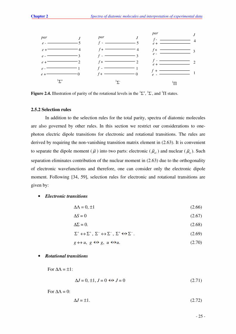
From (2.65) and (2.62) one can see that all rotational levels in 1Σ+ states are of e parity,
while levels in 1Σ- states are of f parity. For singlet states having Λ > 0 (i.e., 1Π, 1∆ ...) each
rotational level is composed of two components, one corresponds to e-parity and the other
corresponds to f-parity. Figure 2.4 illustrates parity of the rotational levels in Σ+, Σ-, and 1Π
states.
Chapter 2 Spectra of diatomic molecules and interpretation of experimental data
- 25 -
Figure 2.4. Illustration of parity of the rotational levels in the 1Σ+, 1Σ-, and 1Π states.
2.5.2 Selection rules
In addition to the selection rules for the total parity, spectra of diatomic molecules
are also governed by other rules. In this section we restrict our considerations to one-
photon electric dipole transitions for electronic and rotational transitions. The rules are
derived by requiring the non-vanishing transition matrix element in (2.63). It is convenient
to separate the dipole moment ( µ
) into two parts: electronic (el
µ
) and nuclear (n
µ
). Such
separation eliminates contribution of the nuclear moment in (2.63) due to the orthogonality
of electronic wavefunctions and therefore, one can consider only the electronic dipole
moment. Following [34, 59], selection rules for electronic and rotational transitions are
given by:
• Electronic transitions
∆Λ = 0, ±1 (2.66)
∆S = 0 (2.67)
∆Σ = 0. (2.68)
+ +Σ ↔ Σ , − −Σ ↔ Σ , +Σ −Σ . (2.69)
g ↔ u, g g, u u. (2.70)
• Rotational transitions
For ∆Λ = ±1:
∆J = 0, ±1, J = 0 J = 0 (2.71)
For ∆Λ = 0:
∆J = ±1. (2.72)
0
1
2
3
4
5
0
1
2
3
4
5
e +
e -
e +
e -
e +
e -
f +
f -
f +
f -
f +
f -
1
2
3
4
f +
f -
f +
f -
e -
e +
e -
e +
J par par par J J
1Π 1Σ- 1Σ+
Chapter 2 Spectra of diatomic molecules and interpretation of experimental data
- 26 -
For e/f parity:
e ↔ f for ∆J = 0 , (2.73)
e ↔ e, f ↔ f for ∆J = ±1. (2.74)
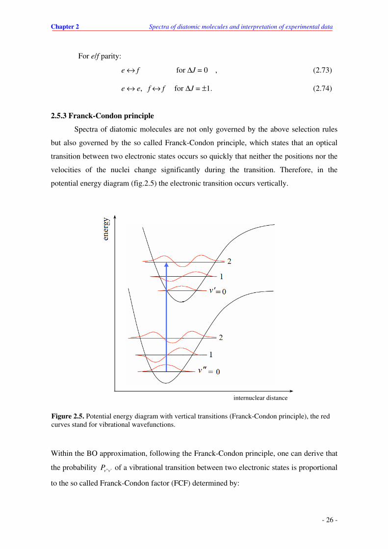
2.5.3 Franck-Condon principle
Spectra of diatomic molecules are not only governed by the above selection rules
but also governed by the so called Franck-Condon principle, which states that an optical
transition between two electronic states occurs so quickly that neither the positions nor the
velocities of the nuclei change significantly during the transition. Therefore, in the
potential energy diagram (fig.2.5) the electronic transition occurs vertically.
Within the BO approximation, following the Franck-Condon principle, one can derive that
the probability " 'v vP of a vibrational transition between two electronic states is proportional
to the so called Franck-Condon factor (FCF) determined by:
internuclear distance
Figure 2.5. Potential energy diagram with vertical transitions (Franck-Condon principle), the red curves stand for vibrational wavefunctions.

Chapter 2 Spectra of diatomic molecules and interpretation of experimental data
- 27 -
' "
22
" ' " '( ) ( )vib vib
v v v v v vP FCF R R dRξ ξ≅ ∫∼ . (2.75)
Here ' ( )vib
vRξ and " ( )vib
vRξ are vibrational wavefunction for level v
' and v
", respectively.
Since the integral (2.75) depends on vibrational wavefunctions and sensitively depends on
vibrational quantum numbers (v', v") as a consequence changes of the transition intensity
within the progressions starting from individual v" is observed. As an example in fig.2.5, is
shown situation where intensity of the transition v' = 0 - v" = 0 is much weaker than that of
the 0 - 2 due to different overlap between corresponding wavefunctions.
2.6. Perturbations in molecular spectra
In principle within the BO approximation it should be possible to deduce position
of all observed spectral lines from potential energy curves. Nevertheless it turns out that it
is not always the case - namely wavelengths of some spectral lines deviate more or less
pronouncedly from that calculated from the potentials. We call these shifted spectral lines
(or levels involved in certain transition) as perturbed. The perturbations in molecular
spectra involve the terms neglected in the total Hamiltonian in the BO approximation.
From the point of view of the perturbation theory one can consider the BO approximation
as the zero-order approximation and take into account the neglected BO terms as higher
order corrections. In general we can represent the total Hamiltonian H by:
ˆ ˆ ˆ ˆel N s= + +H H T H . (2.76)
In (2.76), ˆ elH stands for the electronic Hamiltonian including nuclear repulsion, ˆ NT stands
for the nuclear kinetic operator, and ˆ sH stands for the operator for the spin interactions.
The total energy of the molecule is calculated via the matrix elements of the above
operators in the basis of BO wavefunctions. In particular, the diagonal elements of (2.76)
give the energy of the molecule which we considered in the previous sections, while off-
diagonal elements of (2.76) give rise to perturbations.
2.6.1 Electrostatic and non-adiabatic perturbations
The electrostatic and non-adiabatic perturbations arise from off-diagonal elements
of ˆ elH and ˆ NT operators, respectively [60-63]. From the point of view of the perturbation

Chapter 2 Spectra of diatomic molecules and interpretation of experimental data
- 28 -
theory it is important to choose a basic functions in a way that the off-diagonal matrix
elements,
ˆ ˆ ˆ ˆN N
i k i k i kΨ + Ψ = Ψ Ψ + Ψ Ψel elH T H T (2.77)
are small. Because ˆ elH and ˆ NT operators do not commute there is no way to find a basis
of functions in which both two terms in (2.77) simultaneously vanish. In practice, two
equivalent ways for choosing the basic functions are used to get each term in (2.77)
alternatively vanished. The first, in which the off-diagonal elements of ˆ NT vanish, is
called the diabatic representation. In this representation the no-vanishing off-diagonal
elements of ˆ elH give rise to electrostatic perturbations. The second one is adiabatic
representation where the off-diagonal elements of ˆ elH vanish. In the adiabatic
approximation, off-diagonal elements of ˆ NT give rise to non-adiabatic couplings.
According to Neumann and Wigner any two potential curves of electronic states of
identical symmetry do not cross each other. If in a certain approximation the potential
curves cross each other then higher order corrections (electrostatic or non-adiabatic
couplings) has to be taken into account. The resultant potential curves obtained in these
cases usually have irregular shapes because of the avoided crossing.
In diabatic representation the electrostatic perturbations are represented by the
following matrix elements:
, ; ,ˆ
k l k l
d d d d e
k v l v k v l v k lH H v vχ χ= Φ Φ ≈elH , (2.78)
where
ˆe d d
k lH = Φ ΦelH , and ( )
k l
d d d d
k l v vv v R dRχ χ= ∫ . (2.79)
For most cases, He depends weakly on internuclear separation R. Therefore, using the R-
centroid approximation [61] the off-diagonal matrix elements can be estimated
theoretically.
In adiabatic representation the perturbations are due to the matrix elements of the
kinetic energy operator of the two nuclei. The diagonal matrix element of this operator is
called adiabatic correction, and the off-diagonal matrix elements are called non-adiabatic
couplings. In most cases the magnitude of adiabatic correction is much larger than those of

Chapter 2 Spectra of diatomic molecules and interpretation of experimental data
- 29 -
non-adiabatic couplings. Including the adiabatic correction into the BO potential one
obtains the so called adiabatic potential:
( ) ( )ad BO N
k k kkU R U R T= + . (2.80)
In higher approximations the potential energy of the molecule is calculated by adding
adiabatic potential ( )ad
kU R to the non-adiabatic coupling terms N
klT , where
, : ,ˆ
k l k l
N N ad ad ad ad
kl k v l v k v l vT T χ χ= = Φ ΦN
T . (2.81)
Therefore it is necessary to know adiabatic wavefunctions in order to estimate non-
adiabatic coupling.
2.6.2 Spin-Orbit coupling
In (2.76) the operator ˆ sH can be represented as a sum of the spin-orbit ( ˆ s-lH ) and
the spin-spin ( ˆ s-sH ) interactions. These interactions are responsible for spin perturbations
and usually the spin-orbit interactions are much stronger than that of the spin-spin
interactions. The spin-orbit interactions appear due to coupling among spins of electrons
and the angular momenta caused by moving electrons and the rotating molecule. Let's
consider a case where the couplings between the different angular momenta i
l
of the
electrons and between their spins i
s
are stronger than the interaction between i
l
and i
s
(Hund's case (a)). In this case the ˆ s-lH is approximated by [60-61]:
ˆ A=s-lH
LS with
il∑
L = and i
s∑ S = , (2.82)
where A is the spin-orbit coupling constant. It is then convenient to calculate ˆ s-lH in the
BO basis functions , , , ,S vΛ Σ Ω of Hund's case (a). The matrix elements of ˆ s-lH give the
energies of the fine-structure components. In the next step the higher-order couplings
(i k
s l
and i k
s s
) are introduced. The selection rules for non-vanishing matrix elements
ˆ, , , , , , , ,i i i i i k k k k k
S v S vΛ Σ Ω Λ Σ Ωs-lH (2.83)
of the spin-orbit coupling are following [60-61]:

Chapter 2 Spectra of diatomic molecules and interpretation of experimental data
- 30 -
0; 0, 1; 0.J S∆ = ∆ = ± ∆Ω = (2.84)
Generally only rotational levels with the same total angular momentum quantum number J
can interact through spin-orbit interactions. From the rules in (2.84) we see that, if the two
interacting states belong to the same electron configuration then ∆Λ = ∆Σ = 0 holds. If the
two states differ by one spin orbital then ∆Λ = - ∆Σ = ±1.
2.6.3 Rotational perturbations
The rotational perturbations arise from off-diagonal matrix elements of the
rotational kinetic energy operator. These matrix elements are determined by terms
neglected in BO approximation. In detail, the neglected terms are given by [61]:
2
1 ˆ ˆˆ ˆ( )2 Rµ
+ − − ++L S L S (2.85)
2
1 ˆ ˆˆ ˆ( )2 Rµ
+ − − +− +J S J S (2.86)
2
1 ˆ ˆ ˆ ˆ( )2 Rµ
+ − − +− +J L J L , (2.87)
where ˆ +X and ˆ −
X ( X stands for J , L , S operators) are lowering and rising operators,
respectively. These terms are responsible for the following perturbations:
• Homogeneous spin-electronic perturbation
The homogeneous spin-electronic perturbation arises from the off-diagonal matrix
elements of (2.85). These couplings are non-zero between states having the same Ω and S,
but different Λ and Σ. The selection rules for the spin-electronic perturbations are given by
[61]:
∆Ω = 0, ∆S =0, ∆Λ = -∆Σ = ±1. (2.85a)
Therefore, the spin-electronic perturbation gives rise to local perturbations between
electronic states of different symmetry.
• Heterogeneous electronic-rotation perturbations
The heterogeneous electronic-rotation perturbations arise from the operator (2.86) which is
called S
-uncoupling operator. This operator couples states having different Ω and Σ, but
Chapter 2 Spectra of diatomic molecules and interpretation of experimental data
- 31 -
having the same Λ and S. The heterogeneous electronic-rotation perturbations obey the
following selection rules [61]:
∆Ω = ∆Σ = ±1, ∆S = ∆Λ = 0. (2.86a)
In the heterogeneous electronic-rotation perturbations, the S
-uncoupling operator mixes
different components of the same electronic state, often between the substates of different
vibrational levels. Therefore, it gives rise to local perturbations. When rotation increases,
the S
-uncoupling operator tends to make transition from Hund's case (a) to case (b).
• Heterogeneous electronic-rotation perturbations
The term given by (2.87) is called L
-uncoupling operator. It is responsible for
heterogeneous electronic-rotation perturbations between states having different Ω- and Λ-
values but having the same Σ and S. The selection rules for this type of perturbations are
determined by [61]:
∆Ω = ∆Λ = ±1, ∆S = ∆Σ = 0. (2.87a)
As the rotation of the molecule increases, the L
-uncoupling operator tends to make
transition from Hund's case (a) to case (d), which is called the uncoupling phenomenon.
Upon such interactions the degenerated energy levels in states having Λ > 0 are gradually
split.
For 1П symmetry states, under such interactions the two-fold degenerate levels are
split - this is so called lambda-doubling. According to the selection rules (2.87a) levels in 1П state couple with levels in states of 1Σ+, 1Σ-, and 1∆ symmetry. For a given J, there are
two e- and f-components. If these degenerated levels are coupled by levels in a 1Σ+
electronic state, only e- parity components in 1П state are affected. Alternatively if the
degenerated levels are coupled with levels in a 1Σ- state, only f-parity components in 1П
state are affected. In general, the amplitude of the lambda-doubling splitting depends on
strength of coupling between vibrational and rotational motions. For convenience, such
splitting is often given in terms of double power expansion of vibrational and rotational
quantum numbers. Namely,
12
,
( , ) ( ) [ ( 1)]k l
kl
k l
T v J q v J J∆ = + +∑ , (2.88)
Chapter 2 Spectra of diatomic molecules and interpretation of experimental data
- 32 -
where qkl represent the lambda-doubling coefficients. The representation of the lambda-
doubling splitting in form (2.88) is convenient for cases where spectroscopic term values
are determined by Dunham expansion (2.37) or for construction of potential curve in
numerical form. An alternative form for representing the lambda-doubling splitting is a
function of internuclear distance [58]:
22
2( , ) ( ) ( )
2T v J T R f R
RµΛ
∆ = ∆ =
(2.89)
where ( )f RΛ is a so called lambda-doubling strength function. This representation of
lambda-doubling splitting is convenient for construction of potential curve in analytical
form.

Chapter 3 Polarization labelling spectroscopy and experimental arrangement
- 33 -
Chapter 3
Polarization labelling spectroscopy and experimental
arrangement
3.1. Polarization labelling spectroscopy
3.1.1 Basic principles
The polarization labelling spectroscopy (PLS) method was proposed in 1976 [27]. It
combines polarization spectroscopy and optical-optical double resonance techniques [64-
66]. The basic idea of the method is to monitor changes of polarization of a weak probe
laser beam after passing through a molecular sample optically pumped by a strong laser
light coming from another laser. A typical experimental scheme of PLS experiment is
shown in figure 3.1, where the molecular sample is placed between two crossed linear
polarizers P1 and P2.
Figure 3.1. Scheme of the PLS method: P1 and P2 are the pair of crossed linear polarizers, D is
detector to monitor signal of the probe beam.
Probe Laser
Pump Laser
λ/4 - plate
molecular sample P1
P2 D

Chapter 3 Polarization labelling spectroscopy and experimental arrangement
- 34 -
When the pump laser is off, the molecular sample is optically isotropic because
there is no preferential direction for total angular momentum J of each molecule. Namely
for a given value of quantum number J there are 2J + 1 degenerated Zeeman sublevels,
each has the same statistical weight. Each Zeeman sublevel corresponds to a value of
quantum number MJ which is a quantum number of the projection of J on the propagation
axis of the pump beam. Therefore, the linear polarization of the probe beam is unchanged
after passing through the sample, thus any light from probe laser reaches the detector D.
When the pump beam is on, let’s assume that the wavelength of the pump laser is
tuned to excite molecular transition J" → J
'. Hence, the pump light depopulates the
absorbing molecules at the lower level J" and then populates them to upper level J'. It is
known that the depopulation for the lower level (or the population for the upper level) is
not the same among the Zeeman sublevels because of the two following reasons. The first
one is the selection rules for transitions between Zeeman sublevels: ∆M = 0, +1, or -1 for
linear, right circular-, or left circular polarization, respectively. The second one is
dependence of absorption cross-section on value of MJ, as illustrated in fig.3.2. As a result
the sample becomes anisotropic for the probe light. Therefore, whenever the probe light
excites a transition which shares the lower or upper level with the pumped transition, the
polarization of the probe beam changes and the probe beam passes through the polarizer P2
and reaches the detector. Detail description for anisotropy due to optical pumping can be
found in [64-71].
Figure 3.2. MJ - dependence of absorption cross-section [98]. The notations σ+, σ-, and σo stand for right circular-, left circular-, and linear- polarization, respectively.

Chapter 3 Polarization labelling spectroscopy and experimental arrangement
- 35 -
In the original version of PLS technique [27], wavelength of the probe laser was
tunable whereas that of the pump laser was fixed. Consequently the PLS spectra exhibited
rovibrational structure of electronic states on which probe transitions terminate. An
alternative PLS version used in this work was based on a fixed-wavelength probe laser and
a tunable pump laser [28]. Thus the PLS spectra exhibit rovibrational structure of
electronic states on which pump transitions end on.
So summarizing, whenever the pump light is tuned to the transitions sharing
common level with the probe transition, the polarization of the probe changes slightly. As a
result, sweeping wavelength of the pump laser and monitoring probe light passing through
the analyzer we obtain excitation spectrum of the molecule starting only from the chosen
levels, as it is called labelled by the probe laser. In this way the spectrum is greatly
simplified in comparison to the usual absorption spectrum and consequently, rotational
resolution is obtained even for heavy molecules.
3.1.2 Amplitude of polarization signal
Let assume that the probe light propagates along z -axis and it is polarised in x -
direction (this is the optical axis of the polarizer P1)
exp[ ( )]; ,0,0o o ox
E E i t kz E Eω= − =
. (3.1)
Let us consider the case of the circularly polarized pump light. The electric vector E
of the
probe beam can be decomposed into left and right circularly polarized components in
terms of the following expressions:
12exp[ ( )], ( )
o o o x yE E i t k z E E e ieω+ + + += − = +
(3.2a)
12exp[ ( )], ( )
o o o x yE E i t k z E E e ieω− − − −= − = −
. (3.2b)
Here, x
e
and y
e
are unit vectors in the x and y directions, respectively; E+
and E−
are the
right and left circularly polarized components, respectively. Passing through the sample of
length L the two components experience a birefringence (due to the different refractive
indexes n+ and n-) and dichroism (due to the different absorption coefficients α+ and α-).
Therefore these two components of the probe beam after passing through the sample
become

Chapter 3 Polarization labelling spectroscopy and experimental arrangement
- 36 -
2( ) exp[ ( )]o
E z L E i t k L i Lαω++ + += = − +
, (3.3a)
2( ) exp[ ( )]o
E z L E i t k L i Lαω−+ − −= = − +
. (3.3b)
Superposition of these two components yields an elliptic polarization
E E E+ −= +
[ ]( / / 2)1
02 [( ) ( ) ]i nL c i Li t i i
x y x yE e e e ie e e ie e
ω αω − − ∆ ∆= + + −
. (3.4)
Where,
1 12 2( ); ( )n n n α α α+ − + −= + = +
are the average quantities, and
/ 2 / 4L n c iLω α∆ = ∆ − ∆
is phase factor which depending on the birefringence (∆n) and dichroism (∆α):
;n n n α α α+ − + −∆ = − ∆ = − .
If the transmission axis of the analyser P2 is tilted with a small angle θ << 1 against the y-
axis, the transmitted amplitude of the probe light could be written
sin cost x y x y
E E E E Eθ θ θ= + ≈ + . (3.5)
For most practical cases ∆αL << 1 and ∆nL << 1 thus one can expand exp [i∆] into the
Taylor series, retain the first term, and then substitute into (3.5). The transmitted amplitude
is then given by
12exp[ ]exp[ / ]( )
t oE E i t i nL c Lω ω α θ= − − ∆ . (3.6)
The polarization signal S(ω) at the detector is proportional to the transmitted intensity
given by:
*( ) ( )t o t tS I c E Eω ω ε∝ = ,
2( )L
t oI I e α ξ θ−= + + ∆
2 2
2
4L
o
LI e L n L n
c c
α ω ω αξ θ θ− ∆
= + + ∆ + ∆ +
, (3.7)
where the ξ-coefficient was introduced due to imperfect extinction of the polarizers.

Chapter 3 Polarization labelling spectroscopy and experimental arrangement
- 37 -
On the other hand from the Kramers-Krönig dispersion relation, ∆n can be represented in
terms of ∆α by:
2
( )( ) ( )
1o
o o
xc cn x
x
α ωω α ω
ω ω
∆∆ = ∆ =
+, (3.8)
where
2 2
2( ) ( ), ( )
1 1o o o
s
xx x
ω ω α ω αα ω
γ
− ∆ ∆= ∆ = =
+ +, (3.9)
and ωo central frequency of line with halfwidth γs.
Substituting (3.8) and (3.9) into (3.7) the transmitted intensity can be written as
22
22 2 2
13
1 4 1 4(1 )L o o
t o o
L L xxI I e L
x x x
α α αξ θ θ α− ∆ ∆
= + + ∆ + + + + +
. (3.10)
For the other case of linearly polarized pump light beam, maximum amplitude of
the polarization signal appears when polarization planes of the pump and probe beams are
tilted by 45o. In this case, the electric vector of the probe light could be decomposed into
two components, one parallel and the other perpendicular to the polarization direction of
the pump beam. After passing through the anisotropic sample the two components of the
probe beam also experience the birefringence and dichroism in a similar way to the
previously discussed case of the circularly polarized pump light. Therefore, the transmitted
intensity could be written:
22
22 2 2
13
1 4 1 4(1 )L o o
t o o
L L xxI I e L
x x x
α α αξ θ θ α− ∆ ∆
= + − ∆ + + + + +
, (3.11)
where ∆αo is defined as the difference between α⊥ and α|| for the perpendicular and parallel
components, respectively.
If one tunes the wavelength of the probe laser into resonance and assuming θ = 0 (perfect
crossing of the polarizer) both Eqs.(3.10) and (3.11) are reduced to
2
2
( )
16(1 )L o
t o
LI I e
x
α αξ− ∆
= + +
. (3.12)
The first term in (3.12) represents background signal (Ib) due to the extinction of the
polarizers, and the second term represents the polarization signal (Ip), where:

Chapter 3 Polarization labelling spectroscopy and experimental arrangement
- 38 -
exp( )b o
I I Lξ α= − (3.13a)
2
2
( )xp( )
16(1 )o
p o
LI I e L
x
αα
∆= −
+ . (3.13b)
At the resonance, a signal-to-background ratio can be estimated by
2
2 ( )16
p o
B
IL
I
α
ξ
∆= . (3.14)
Typical extinction of good quality polarizers is better than 10-6 and the sensitivity of
polarization spectroscopy is therefore greater several orders of magnitude in comparison to
that of saturation spectroscopy [64].
3.1.3 Excitation schemes
There are five types of excitation scheme [69-70] which can give rise to
polarization signal, as illustrated in figure 3.3.
In the type 1, also called V-type scheme, the pump and probe transitions share
lower common rovibrational level in the ground electronic state. If wavelength of the probe
light is fixed whereas that of pump laser is tuned over investigated spectral range, the
polarization spectrum exhibits rovibrational structure of the upper electronic state in which
the pumped transitions terminate.
In the type 2, also called Λ-type scheme, the pump and probe transitions share
upper common rovibrational level, and the probe light dumps the pumped molecules into
the rovibrational level in the lower electronic state. In this scheme, wavelength of the probe
beam is tuned, thus the PLS spectrum reveals rovibrational structure of the electronic state
in which the probe transition ends.
The transition scheme via type 3 is called step-wise scheme and occurs when the
molecules in the upper level of the pumped transition absorb a photon of the probe light
and they are excited to the higher levels. The step-wise PLS spectrum exhibits
rovibrational structure of the electronic state in which the probe transition end.
After absorption of the pump-photon fluorescence to lower state occurs and
populates unequally Zeeman sublevels in lower rovibrational levels (type 4 in fig. 3.3). If
the probe beam excites molecules from one of these levels the polarization signal appears.
If we have high density of molecules or high pressure of inert (buffer) gas,
collisional energy transfer between the pumped level and nearby rotational levels can be

Chapter 3 Polarization labelling spectroscopy and experimental arrangement
- 39 -
efficient. Such process leads also to unequal populations of Zeeman sublevels and gives
rise to polarization signal following scheme 5 in fig. 3.3.
Figure 3.3. Excitation schemes in polarization labelling spectroscopy.
Actually PLS signals due to transitions via 4 and 5 types are rarely met in literature.
Depending on particular purposes 1, 2, and 3 types are rather used. For instances, the Λ-
type can be used to investigate the ground electronic state [32] while the V-type, and step-
wise type is preferentially used for excited and Rydberg electronic states [33, 69].
3.1.4 Relative intensities of spectral lines
This section outlines expressions for relative intensities of spectral lines in V-type
PLS scheme. Let us consider wavelength of the probe beam tuned to the centre of the line
profile and let us neglect the background signal due to finite extinction of polarizers.
Following (3.13b), the intensity of the polarization signal is given as
type 1 (V-type)
pump
type 2 (Λ- type)
pump
probe
type 3 (two-step type)
pump
probe
type 4
pump
probe
type 5
pump probe
non-radiative relaxation
probe

Chapter 3 Polarization labelling spectroscopy and experimental arrangement
- 40 -
2
2( )xp( ) ( )
16o
p o o
LI I e L
αα α
∆= − ∝ ∆
. (3.15)
By introducing notation for the set of quantum numbers of the levels (Λk, Jk, Mk),
where k = 1 for upper level of the pumped transition, k = 2 for the upper level of the
probing transition, and k is omitted for the common lower level, the authors in [72] derived
expressions of ∆αo for cases of circularly and linearly polarized pump light as follows:
1 2
1 2 2 1
( ) ( )
1 1(2 1)(2 1)C Co
o J J J J J J JS SJ J
σα α α ζΛ Λ Λ Λ+ − ∆
∆ = − =+ +
(3.16a)
1 2
1 2 2 1
( ) ( )
1 1(2 1)(2 1)C z x Lo
o J J J J J J JS SJ J
σα α α ζΛ Λ Λ Λ∆
∆ = − =+ +
. (3.16b)
In these expressions the superscripts C and L denote the circular and linear polarizations of
the pump beam, respectively; oσ∆ is a parameter depending on product of electronic
transition dipole moment and the Franck-Condon factor; S is the Hönl-London factor
describing intrinsic line strength of rotational intensity:
1
1
2
11
1 1
1(2 1)(2 1)JJ
J JS J J
ΛΛ = + +
−Λ Λ − Λ Λ . (3.17)
The ζ -factor describes the dependence of line intensity on "spatial distribution" of the
angular momentum due to the optical pumping:
2 1
2 1
( )
2 2 2
1 2 2
1 2 2
(2 1)
1 1 1
1 1 1M M M
C
J J J oA J
J J J J J J
M M M M M M
ζ = +
× −
− − − − ∑
(3.18a)
2 1
2 1
2
1( )
1
2 2 2
2 2 2
2 2 2
1(2 1)
0
1 1 11.
0 1 12
M M M
L
J J J o
J JA J
M M
J J J J J J
M M M M M M
ζ
= + × −
× − −
− − − −
∑ (3.18b)
In the above expressions, the Wigner 3j-symbols are used, and the summations are carried
out over the M-sublevels.

Chapter 3 Polarization labelling spectroscopy and experimental arrangement
- 41 -
For diatomic molecules having the ground states of 1Σ+-symmetry, the selection
rules (presented in chapter 2) show that the upper electronic states of the pumped or probe
transitions are either of 1Σ+ or 1Π - symmetry. Thus the relative intensities between spectral
lines can be derived by substituting expressions (3.16) - (3.18) into (3.15). Tables 3.1- 3.4
list relative intensities for P, Q, and R branches with all possible combinations of the probe
and pump transitions, where for the sake of simplicity we present square roots of
intensities [72].
Table 3.1. Relative intensities ( I ) in PLS spectrum when pumping via the 1Π ← 1Σ+ band.
Probe via 1ΠΠΠΠ ←←←←
1ΣΣΣΣ+
Pump
P line Q line R line
Cir – P line 2
3( 1) ( 1) 3
8 (2 1)(2 1) 32
J J
J J J
− +→
− +
3( 1)0
8 (2 1)
J
J J
−→
−
3( 1)( 2) 3
8(2 1)(2 1) 32
J J
J J
− +→
− +
Cir – Q line 3( 1)
08 (2 1)
J
J J
−→
+
30
8 ( 1)J J→
+
3( 2)0
8( 1)(2 1)
J
J J
+→
+ +
Cir – R line 3( 1)( 2) 3
8(2 1)(2 3) 32
J J
J J
− +→
+ +
3( 2)0
8( 1)(2 3)
J
J J
+→
+ +
23 ( 2) 3
8( 1)(2 1)(2 3) 32
J J
J J J
+→
+ + +
Lin – P line 2
23( 1) ( 1)(2 3) 3
40 (2 1) (2 1) 160
J J J
J J J
− + +→
− +
3( 1)(2 3) 3
40 (2 1) 40
J J
J J
− +→
−
3( 1)( 2) 3
40 (2 1)(2 1) 160
J J
J J J
− +→
− +
Lin – Q line 3( 1)(2 3) 3
40 (2 1) 40
J J
J J
− +→
+
3(2 1)(2 3) 3
40 ( 1) 10
J J
J J
− +→
+
3( 2)(2 1) 3
40( 1)(2 1) 40
J J
J J
+ −→
+ +
Lin – R line 3( 1)( 2) 3
40 (2 1)(2 3) 160
J J
J J J
− +→
+ +
3( 2)(2 1) 3
40( 1)(2 3) 40
J J
J J
+ −→
+ +
2
2
3 ( 2) (2 1) 3
40( 1)(2 1)(2 3) 160
J J J
J J J
+ −→
+ + +
Table 3.2. Relative intensities ( I ) in PLS spectrum when pumping via the 1Σ+ ← 1Σ+ band. Probe via
1ΠΠΠΠ ←←←← 1ΣΣΣΣ+
Pump
P line Q line R line
Cir - P line 3( 1)( 1) 3
4(2 1)(2 1) 16
J J
J J
− +→
− +
30
4(2 1)J→
−
3 ( 2) 3
4(2 1)(2 1) 16
J J
J J
+→
− +
Cir - R line 3( 1)( 1) 3
4(2 1)(2 3) 16
J J
J J
− +→
+ +
30
4(2 3)J→
+
3 ( 2) 3
4(2 1)(2 3) 16
J J
J J
+→
+ +
Lin - P line 2
3( 1)( 1)(2 3) 3
20(2 1) (2 1) 80
J J J
J J
− + +→
− +
3(2 3) 3
20(2 1) 20
J
J
+→
−
3 ( 2) 3
20(2 1)(2 1) 80
J J
J J
+→
− +
Lin - R line 3( 1)( 1) 3
20(2 1)(2 3) 80
J J
J J
− +→
+ +
3(2 1) 3
20(2 3) 20
J
J
−→
+ 2
3 ( 2)(2 1) 3
20(2 1)(2 3) 80
J J J
J J
+ −→
+ +

Chapter 3 Polarization labelling spectroscopy and experimental arrangement
- 42 -
Table 3.3. Relative intensities ( I )in PLS spectrum when pumping the 1Π ← 1Σ+ band. Probe via
1ΣΣΣΣ+ ←←←←
1ΣΣΣΣ+ Pump
P line R line
Cir - P line 3( 1)( 1) 3
4(2 1)(2 1) 16
J J
J J
− +→
− +
3( 1)( 1) 3
4(2 1)(2 1) 16
J J
J J
− +→
− +
Cir - Q line 30
4(2 1)J→
+
30
4(2 1)J→
+
Cir - R line 3 ( 2) 3
4(2 1)(2 3) 16
J J
J J
+→
+ +
3 ( 2) 3
4(2 1)(2 3) 16
J J
J J
+→
+ +
Lin - P line 2
3( 1)( 1)(2 3) 3
20(2 1) (2 1) 80
J J J
J J
− + +→
− +
3( 1)( 1) 3
20(2 1)(2 1) 80
J J
J J
− +→
− +
Lin - Q line 3(2 3) 3
20(2 1) 20
J
J
+→
+
3(2 1) 3
20(2 1) 20
J
J
−→
+
Lin - R line 3 ( 2) 3
20(2 1)(2 3) 80
J J
J J
+→
+ + 2
3 ( 2)(2 1) 3
20(2 1)(2 3) 80
J J J
J J
+ −→
+ +
Table 3.4. Relative intensities ( I )in PLS spectrum when pumping via the 1Σ+ ← 1Σ+ band.
Probe via 1ΣΣΣΣ+
←←←← 1ΣΣΣΣ+
Pump
P line R line
Cir - P line 3 ( 1) 3
2(2 1)(2 1) 8
J J
J J
+→
− +
3 ( 1) 3
2(2 1)(2 1) 8
J J
J J
+→
− +
Cir - R line 3 ( 1) 3
2(2 1)(2 3) 8
J J
J J
+→
+ +
3 ( 1) 3
2(2 1)(2 3) 8
J J
J J
+→
+ +
Lin - P line 2
3 ( 1)(2 3) 3
10(2 1) (2 1) 40
J J J
J J
+ +→
− +
3 ( 1) 3
10(2 1)(2 1) 40
J J
J J
+→
− +
Lin - R line 3 ( 1) 3
10(2 1)(2 3) 40
J J
J J
+→
+ + 2
3 ( 1)(2 1) 3
10(2 1)(2 3) 40
J J J
J J
+ −→
+ +
3.2. Experimental
3.2.1 Preparation of NaLi molecules
Production of NaLi molecules from metallic Na and Li bulks encounters a
difficulty because of the big difference in melting-points of both substances (T1= 180.54oC
for Li and T2= 97.8oC for Na) and consequently big difference in concentration of Na and
Li atoms in the saturated vapour. In order to overcome such difficulty we used the three-
section heat-pipe, which was proposed in [73] to form NaLi molecules. The main
arrangement of the apparatus (fig.3.4) is briefly described below.

Chapter 3 Polarization labelling spectroscopy and experimental arrangement
- 43 -
The heat-pipe oven is made from a stainless steel pipe which is surrounded by three
heaters connected to the separated power supplies that allow independent control of the
temperature of each heater. The temperature of the each section of the pipe is measured
with a chromel-alumel thermocouple placed between the heater and the pipe wall. At both
ends, the pipe is closed with fused silica windows which are fixed by easily demountable
clamped flanges. The windows are kept by rubber O-rings and adjustable screws which
allow compensation of residual birefringence by gently squeezing. Both windows are tilted
against the tube axis in order to eliminate multi-reflection between the windows. Two
stainless steel pipes are welded at the ends of the pipe for connection to vacuum systems.
At each end of the pipe two water-cooler rings are soldered. Three layers of steel mesh are
inserted into the tube in order to assure circulation of the liquid metal by capillary forces.
The mesh matches the distance between the water coolers. A metallic Li is loaded to the
central part of the heat-pipe while Na is placed at outer parts. About 4 Torr of Helium is
filled into the pipe as buffer gas.
Figure 3.4. The three-section heat-pipe oven.
It was found that the best stable condition for forming NaLi molecules can be
achieved with the temperature T1 = 650oC (for the central heater) and T2 = 390oC (for the
outer ones). The NaLi molecules were produced mainly in the central zone of the pipe and
could be maintained in several hours, which was enough long time for us to perform
measurements.
Chapter 3 Polarization labelling spectroscopy and experimental arrangement
- 44 -
3.2.2 Laser sources
a. Pump lasers
The purpose of our experiments was to investigate electronic states of NaLi in a
wide spectral energy range, from 24500 up to 36000 cm-1 by V-type PLS. In order to cover
such spectral energy range we used two pump laser systems. The first one based on dye
laser whereas the second based on optical parametric oscillator/amplifier (OPO/OPA).
• Dye laser system.
The dye laser system was the Lumonics HD 500 operating on BBQ, Butyl PBD,
and BBD dyes pumped by a 308 nm XeCl excimer laser. The dye laser scans were
controlled by a remote controller or by a software equipped computer. This laser generates
light pulses with pulse energy of about 2 mJ, width 8 ns, and linewidth of less than 0.1
cm-1. Using three dyes mentioned above laser system was tunable in the 24500-27800 cm-1
spectral range.
• OPO/OPA- Frequency doubler system.
The system consists of Nd:YAG (3rd harmonic, 355nm) pumped optical parametric
oscillator/amplifier (OPO/OPA) and a frequency doubler. The laser system can be
controlled from a computer via RS-232 interface to scan wavelength in desired spectral
ranges. It generated light-pulses with energy of about 4 mJ, 10 Hz repetition rate and
linewidth of 0.15 cm-1. With this system wavelength of radiation was tunable in 28900 -
40000 cm-1 spectral range.
b. Probe lasers
The probe laser was either a multi-mode CW ion Ar+ laser (Carl Zeiss ILA 120) or
a home-built Littman type dye laser. The Ar+ laser was set at 496.5 nm line with power of
about 40 mW. This laser line excites the 11Π(1, 29) ← 11Σ+(0, 30) transition what was
known from literature in previous measurements in laboratory [16, 17]. The home-built
Littman type laser operated on DCM dye, and was pumped by either the excimer or
Nd:YAG laser. The dye laser generated radiation with energy pulse of about 0.003 mJ and
was tuned to excite desired transitions via the 21Σ+ ← 11Σ+ band system [15-16]. The laser
lines corresponding to the particular probe transition are listed in table 3.5.

Chapter 3 Polarization labelling spectroscopy and experimental arrangement
- 45 -
Table 3.5. The laser lines used in this work as a probe.
laser line probe transition (v’, J
’) ← (v”, J
”)
496.5 nm 11Π(1, 29) ← 11Σ+(0, 30)
15293.3 cm-1 21Σ+(8, 20) ← 11Σ+(1, 21)
15413.0 cm-1 21Σ+(9, 28) ← 11Σ+(0, 29)
15440.2 cm-1 21Σ+(9, 24) ← 11Σ+(1, 25)
15463.8 cm-1 21Σ+(9, 20) ← 11Σ+(1, 21)
21Σ+(11,55) ← 11Σ+(1, 56)
15484.2 cm-1 21Σ+(9,16) ← 11Σ+(1, 17)
15493.5 cm-1 21Σ+(8, 28) ← 11Σ+(0, 29)
21Σ+(9,46) ← 11Σ+(0, 47)
15521.2 cm-1 21Σ+(8,24) ← 11Σ+(0, 25)
21Σ+(9,11) ← 11Σ+(1, 10)
15544.8 cm-1 21Σ+(8, 20) ← 11Σ+(0, 21)
15560.6 cm-1 21Σ+(8, 17) ← 11Σ+(0, 18)
21Σ+(9,44 ) ← 11Σ+(0, 45)
15565.4 cm-1 21Σ+(8,16)← 11Σ+(0, 17)
3.2.3 Experimental arrangement
Depending on which pump laser was used, our experimental setup was arranged as
shown either in fig 3.5 or in fig. 3.6. In each arrangement the pump and probe laser beams
passed nearly collinearly through the heat-pipe oven. Before and after the heat- pipe, two
Glan-Thomson polarizers (P1, P2) were placed on the optical path of the probe beam.
These polarizers were fixed in rotating mounts for fine tuning of their optical axes. In order
to measure the wavelength of the probe beam, a small amount of radiation, extracted with
the beam splitter from the main beam, was directed into a WS5-wavelength meter. The
change of the polarization (circular or linear) of the pump beam was obtained by inserting
a λ/4 Fresnel rhomb before the heat-pipe into the optical path of the pump beam. The PLS
signal after the polarizer P2 was registered with a photomultiplier tube. Before the
photomultiplier, a monochromator was placed to suppress scattered light and fluorescence
outgoing from the heat-pipe oven. The signal from the photomultiplier was measured by a
Stanford SR 250- boxcar averager.
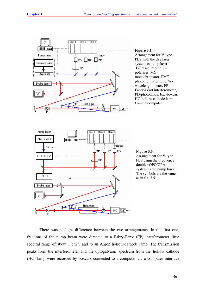
Chapter 3 Polarization labelling spectroscopy and experimental arrangement
- 46 -
Figure 3.5. Arrangement for V-type PLS with the dye laser system as pump laser. F-Fresnel rhomb, P-polarizer, MC-monochromator, PMT-photomultiplier tube, W-wavelength meter, FP-Fabry-Pérot interferometer, PD-photodiode, bxc-boxcar, HC-hollow cathode lamp, C-microcomputer.
Figure 3.6. Arrangement for V-type PLS using the Frequency doubler-OPO/OPA system as the pump laser. The symbols are the same as in fig. 3.5.
There was a slight difference between the two arrangements. In the first one,
fractions of the pump beam were directed to a Fabry-Pérot (FP) interferometer (free
spectral range of about 1 cm-1) and to an Argon hollow-cathode lamp. The transmission
peaks from the interferometer and the optogalvanic spectrum from the hollow cathode
(HC) lamp were recorded by boxcars connected to a computer via a computer interface
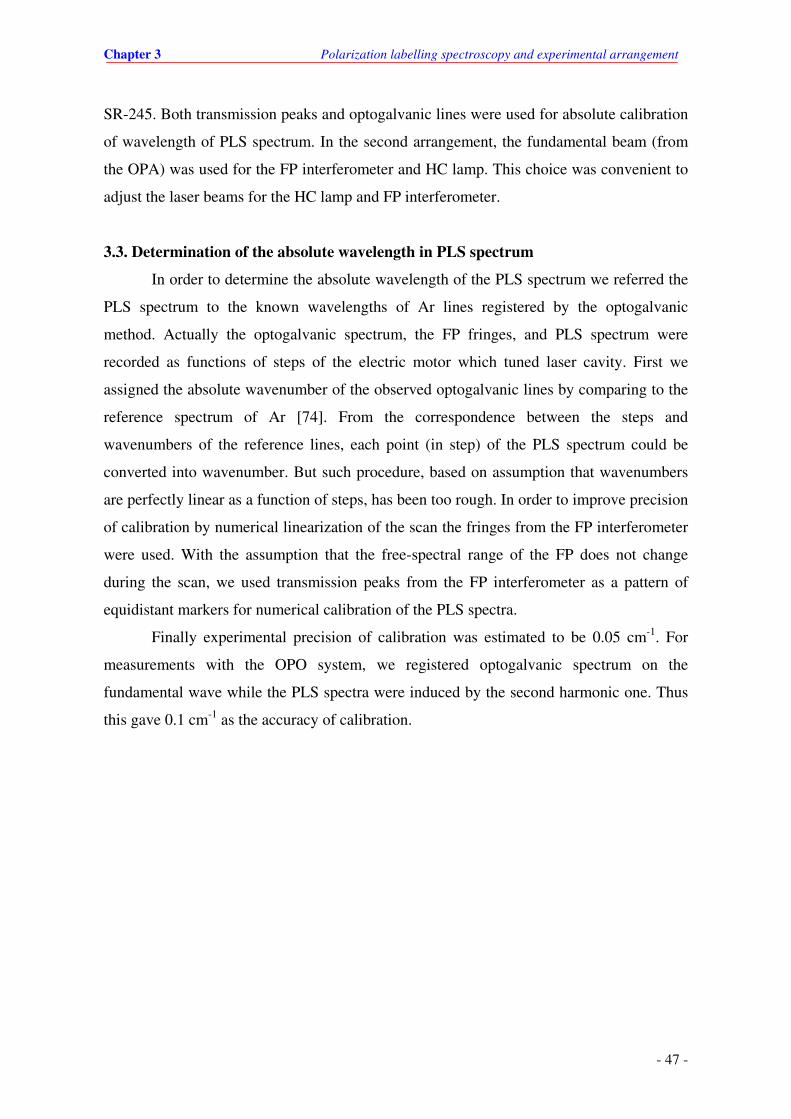
Chapter 3 Polarization labelling spectroscopy and experimental arrangement
- 47 -
SR-245. Both transmission peaks and optogalvanic lines were used for absolute calibration
of wavelength of PLS spectrum. In the second arrangement, the fundamental beam (from
the OPA) was used for the FP interferometer and HC lamp. This choice was convenient to
adjust the laser beams for the HC lamp and FP interferometer.
3.3. Determination of the absolute wavelength in PLS spectrum
In order to determine the absolute wavelength of the PLS spectrum we referred the
PLS spectrum to the known wavelengths of Ar lines registered by the optogalvanic
method. Actually the optogalvanic spectrum, the FP fringes, and PLS spectrum were
recorded as functions of steps of the electric motor which tuned laser cavity. First we
assigned the absolute wavenumber of the observed optogalvanic lines by comparing to the
reference spectrum of Ar [74]. From the correspondence between the steps and
wavenumbers of the reference lines, each point (in step) of the PLS spectrum could be
converted into wavenumber. But such procedure, based on assumption that wavenumbers
are perfectly linear as a function of steps, has been too rough. In order to improve precision
of calibration by numerical linearization of the scan the fringes from the FP interferometer
were used. With the assumption that the free-spectral range of the FP does not change
during the scan, we used transmission peaks from the FP interferometer as a pattern of
equidistant markers for numerical calibration of the PLS spectra.
Finally experimental precision of calibration was estimated to be 0.05 cm-1. For
measurements with the OPO system, we registered optogalvanic spectrum on the
fundamental wave while the PLS spectra were induced by the second harmonic one. Thus
this gave 0.1 cm-1 as the accuracy of calibration.
Chapter 4 Experimental results for the NaLi molecule
- 48 -
Chapter 4
Experimental results for the NaLi molecule
4.1. Introduction
4.1.1 Historical overview of investigations of NaLi
The electronic structure of NaLi was explored theoretically for the first time by
Bertoncini et al [19] in 1970, where authors performed ab initio calculations by using the
multiconfiguration self-consistent field method. They computed four potential curves for
the 11Σ
+, 13Σ
+ 11Π, and 13
Π states and the dipole moment for the ground state. Their results
anticipated that the NaLi molecule, which had not been observed spectroscopically until
that time, is physically stable with dissociation energy of 6850 cm-1 in the ground state.
Later, Green [20] performed calculations of electric dipole moment for the ground state
within the framework of the configuration interaction (CI) theory. The author revealed that
the value of the dipole moment obtained in [19], which was 1.24 debye, is too large owing
to neglect in the previous calculations of contributions from core-polarization effects.
Green’s prediction was later tested experimentally by Graff, Dagdigian and Wharton [25-
26], and results showed that the value of the dipole moment in the electronic ground state
of NaLi is only 0.46 debye. In the following years the dynamical core-polarization effects
in alkali dimer species were taken into consideration by Meyer’s group [21-23]. The
authors introduced operators which are responsible for the core-core and valence-core
interactions into the standard Hamiltonian of the self-consistent field method. Upon these
considerations they computed potential energy curves and some main spectroscopic
constants for the electronic ground state of several alkali dimers, including NaLi. By using
this method, Schmidt-Mink et al [24] computed potential energy curves and spectroscopic
constants for the first sixteen singlet and triplet electronic states of NaLi. The calculated
spectroscopic constants for the first six singlet states (11Σ+, 21Σ+, 11Π, 21Π , 31Σ+, and
41Σ+) were then confirmed by experimental works [12-18] with good overall agreement.
Very recently, Mabrouk et al [79] treated the first forty electronic states of NaLi by using

Chapter 4 Experimental results for the NaLi molecule
- 49 -
Figure 4.1. The PECs of the 1-71Π and 1-101
Σ+ states of NaLi calculated by Mabrouk et al [79].
The blue curves stand for 1Σ+ states, and the red ones for 1Π states.
the parameterized l-dependent polarization potential and full configuration interaction
calculations. Their values of spectroscopic constants for several electronic states were
compared to those obtained in previous experiments, including the 31Π and 41
Π states
observed for the first time in our work. The comparison showed very good agreement with
experimental results to within 1.3% relative error. In figure 4.4 we plotted all computed
PECs of singlet states from [79].

Chapter 4 Experimental results for the NaLi molecule
- 50 -
On the experimental side, the spectroscopic study of rovibrational structure in
electronic states of NaLi encounters two drawbacks. The first one is the difficulty in
producing sufficiently stable concentration of NaLi molecules in the vapour phase. The
second one is overlap of the NaLi spectra with spectra of Na2 and Li2 which makes their
interpretation very difficult. Therefore, despite several attempts since 1928 (see [10] and
references therein), the spectrum of NaLi has not been observed until in 1971 Hessel [11]
demonstrated for the first time experimental observation of spectrum of NaLi molecule by
using laser-induced fluorescence (LIF). He observed fluorescence of transitions assigned to
the 11Π →11Σ+ band system after excitation with the 496 nm Ar+ laser line. Since then
several groups performed experiments to explore rovibrational structure in electronic states
of NaLi. Much attention was focused on the ground state [12, 14-15], and the most
accurate measurements were carried out by Fellows [15]. He used the LIF technique
combined with Fourier transform spectroscopy and observed over 6400 spectral lines up to
almost the dissociation limit of the ground state (experimental data covered 99.5% of the
potential well depth). This resulted in determination of spectroscopic constants and the
rotationless potential energy curve. For excited states, Kappe et at [13] used two-photon
ionization techniques to access vibrational structure of the 21Σ+, 21Π, 31Σ+, 41Σ+, and 51Σ+
states. Since the experiment was carried out at low resolution (typically 2 cm-1), this
allowed determination of only a number of molecular constants (Te, ωe, ωexe, and De), in
particular without rotational constants. Next, Fellows [16] reinvestigated the 21Σ+ state by
means of the LIF combined with Fourier transform spectroscopy, and determined
molecular constants and the RKR potential. Latter, the same technique was used again by
Fellows et al [17] to reinvestigate the 11Π and 31Σ+ states. Perturbations in spectra of 11Π
and 31Σ+ as well as energy transfer from 11Π to 31Σ+ were experimentally confirmed.
Recently, Jastrzębski et al [18] performed experiments to investigate the 41Σ+ state. Those
authors used the V-type PLS technique in which the 496.5 nm Ar+ laser line was used as a
probe light beam to explore the rovibrational structure of the 41Σ+ state. A progression of
first ten vibrational levels in the 41Σ+←11Σ+ (0, 30) band, which consists of two P and R
doublets, was identified. Even though data set acquired in that work was rather sparse it
was still the first experiment able to resolve the rotational structure in the 41Σ+ state of the
NaLi molecule.

Chapter 4 Experimental results for the NaLi molecule
- 51 -
4.1.2 Outline of the electronic states observed in this work
In this work we focussed on investigations of excited electronic states of the NaLi
molecule, particularly the states which were not observed before. We performed V-type
PLS experiments to observe transitions over a wide spectral energy range, from 26000 to
36300 cm-1, and found spectral lines of transitions from the ground state to several 1Σ+ and 1Π states.
The spectra of the lowest 1Σ+- symmetry state observed in this work were found in
the range 26000-27500 cm-1. We readily identified this state as the 41Σ+ (see sect.4.3) since
preliminary molecular constants for this state were known from a previous experiment
[18].
We have also found several spectral lines in the range 28900 - 36000 cm-1
belonging to the 51Σ+, 61Σ+, 71Σ+, 81Σ+, 91Σ+, and 101Σ+ states which are expected in this
region on the basis of theoretical calculations. However the observed lines did not form
any regular pattern because of very irregular shapes of the potential energy curves for the 1Σ+ states (fig. 4.1) and the unambiguous assignment and interpretation was not possible.
Therefore we have concentrated on 1Π states which gave rise to much more regular
spectral patterns making their analysis possible. Finally we have identified observed states
as 31Π, 41Π, 61Π and 71Π. In order to perform such assignment first we compared
experimentally determined electronic energy Te obtained for each state with theoretical
predictions. Such preliminary assignment gave also atomic asymptotes for each state,
following theoretical calculations [79]. With Te = 29981.6, 31179.0, 34042.3, 34535.8 and
35985.4 cm-1 (section 4.4 - 4.6) obtained for successive states of 1Π-symmetry we assigned
the observed states as:
31Π → asymptotically correlated to Na(32D) + Li (22S) (4.1)
41Π → Na(42P) + Li (22S) (4.2)
61Π → Na(32S) + Li (32D) (4.3)
71Π → Na (32P) + Li (22P) (4.4)
Having this assignment and knowing the dissociation energy of the ground state
1[1 ]eD
+Σ = 7105.5 cm-1 [15] and energy of atomic levels [75] we could calculate the
dissociation energy (De) of each state. Since dissociation energies were independently
determined in the theoretical paper [79] this gave additional support for the assignment
(4.1) ÷ (4.4). Following (4.1) ÷ (4.4) we obtained the dissociation energy for each state:

Chapter 4 Experimental results for the NaLi molecule
- 52 -
1 2 2 1 1[3 ] [Na(3 D 3 S)] [1 ] [3 ]e e
eD v D T
+Π = − + Σ − Π = 6296.8 cm-1 (4.1a)
1 2 2 1 1[4 ] [Na(4 3 )] [1 ] [4 ]e e
eD v P S D T+Π = − + Σ − Π = 6193 cm-1 (4.2a)
1 2 2 1 1[6 ] [Li(3 2 )] [1 ] [6 ]e e
eD v D S D T+Π = − + Σ − Π = 4346 cm-1 (4.3a)
1 2 2 2 2 1 1
1
[7 ] [Li(2 2 )] [Na(3 3 )] [1 ] [7 ]
4429cm .
e e
eD v P S v P S D T+
−
Π = − + − + Σ − Π
= (4.4a)
Comparison of our values for electronic and dissociation energies with those calculated in
the theoretical paper [79] shows good agreement (deviations are smaller than 24 cm-1 for Te
and then 61 cm-1 for De), and demonstrates consistency between our assignment for the
observed electronic states and assignment in [79]. However, it is surprising that the above
assignment leads to missing observation of the 51Π state even though we did observations
throughout the whole spectral region between the 31Π and 71Π states. Discussion of the
missing observation of the 51Π state is presented at the end of this chapter.
4.2. Methods of data analysis
In order to derive molecular constants of an electronic state, the experimental term
values/level energies were fitted to the Dunham formula by using the linear least-squares
method. The fitted Dunham coefficients were derived by minimizing the following
quantities:
1. Standard error of the individual coefficient.
2. Deviation between the calculated and experimental values for each line.
3. The dimensionless root mean square deviation, DRMSD, which is given by
122
1
( ) ( )1( )
Nobs cal
i
v i v iDRMSD
N u i=
− = ∆ ∑ , (4.5)
where N is the number of the observed lines, ∆u (i) is experimental uncertainty
which is taken to be 0.1cm-1 for our work, ( )obs
v i and ( )cal
v i are the measured
and calculated wavenumbers of the ith transition, respectively.
In practice, the number of Dunham coefficients is not defined a priori. If the
number of coefficients is large this leads to small DRMSD, but increase the error
(ambiguity) of determined coefficients, so we search for the optimal set of Dunham
coefficients looking for the minimum of all above listed quantities.

Chapter 4 Experimental results for the NaLi molecule
- 53 -
For the construction of a potential energy curve by the IPA technique also the linear
least squares method is used to determine coefficients for the potential correction. Since in
this technique the minimization for the DRMSD leads to an over-determined system of
equations of unknown coefficients, therefore the singular value decomposition (SVD)
method [76] is used.
For construction of a potential curve by the DPotFit technique [58] the nonlinear
least squares method has to be used because in the DPotFit the eigenvalues of the RSE are
nonlinearly dependent on unknown coefficients of a chosen analytical potential function.
Therefore, unlike in the linear least squares method, in the nonlinear least squares one
needs trial values for the unknown coefficients and then it goes to search iteratively
corrections for these coefficients until a convergence is obtained.
4.3. The 4 1ΣΣΣΣ+
state
4.3.1 Observation and assignment of the spectra
Spectra of the 41Σ+ state of NaLi were observed in region 26000-28000 cm-1 for
various labelled levels (table 3.5) in the ground electronic state. The pump light was
delivered by a 308nm excimer laser-pumped HD 500 dye laser, and was circularly
polarized.
Although the 41Σ+ state was already characterized with some preliminary molecular
constants [18] within the current experiment we improved significantly its description by
enlarging almost 10 times number of lines used for analysis. Finally we identified 190
spectral lines of the 41Σ+ ← 11Σ+ band, spanning the range v = 0 -11, J = 9 - 46 in 41Σ+.
The theoretical calculation of Schmidt-Mink et al [24] shows that the 41Σ+ state is
characterized by a double minimum potential; all presently observed levels are confined in
the inner potential well and their numbering follows the progression in this well.
Figure 4.2 shows a part of PLS spectrum in the case of 15486.1 cm-1 probe laser
line. This laser line excites three transitions corresponding to the three labelled levels,
(0, 30), (1, 21) and (1, 40) in the ground state. In fig. 4.4, the distribution of the data in the
field of rotational and vibrational quantum numbers in the 41Σ+ state is plotted.
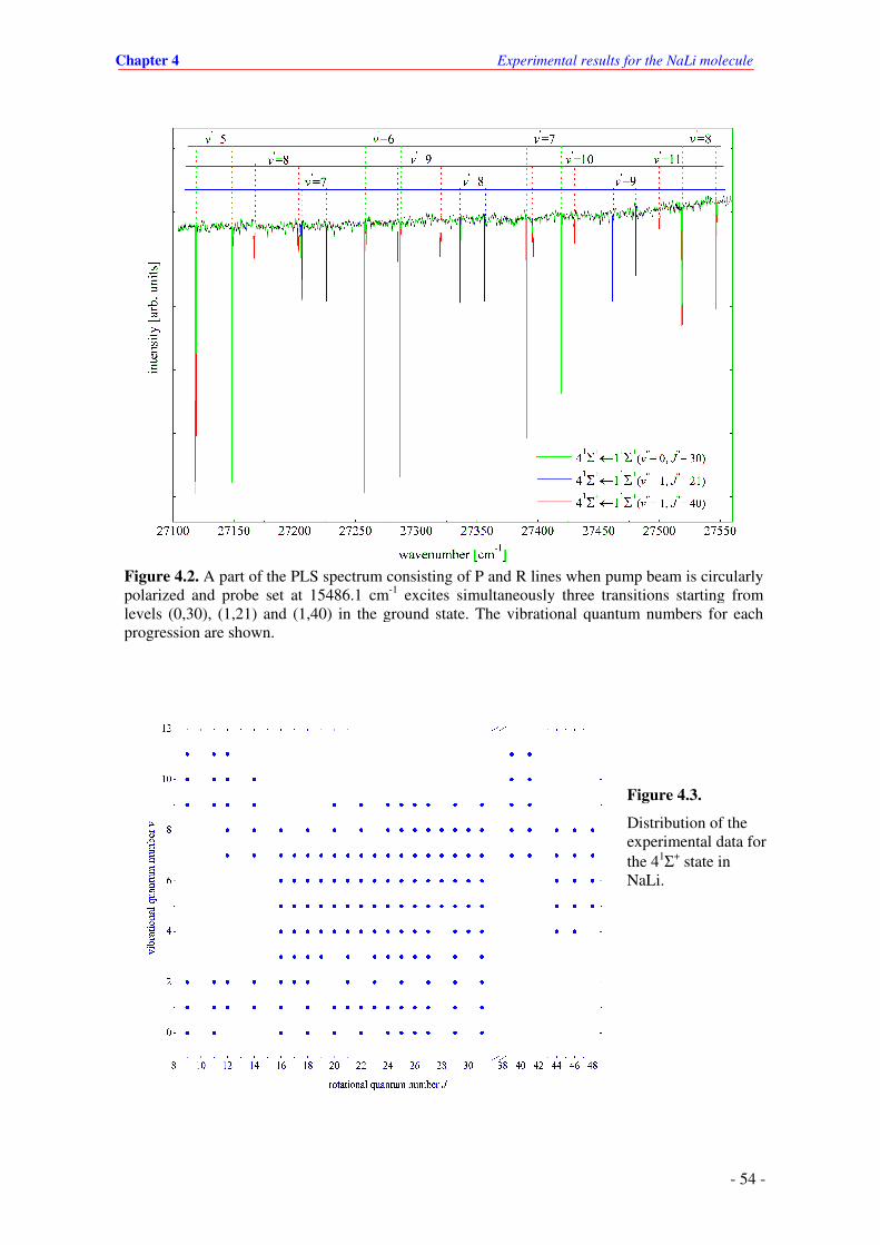
Chapter 4 Experimental results for the NaLi molecule
- 54 -
Figure 4.2. A part of the PLS spectrum consisting of P and R lines when pump beam is circularly polarized and probe set at 15486.1 cm-1 excites simultaneously three transitions starting from levels (0,30), (1,21) and (1,40) in the ground state. The vibrational quantum numbers for each progression are shown.
Figure 4.3.
Distribution of the experimental data for the 41Σ+ state in NaLi.

Chapter 4 Experimental results for the NaLi molecule
- 55 -
4.3.2 Molecular constants
In order to derive molecular constants for the 41Σ+ state the wavenumbers of all
observed spectral lines were fitted to the formula:
' ' ' " " "( , ) ( , )v T v J T v J= − , (4.6)
where T' and T" are the spectroscopic term values of the investigated and ground electronic
states, respectively. The term values for the labelled levels were calculated by using
Dunham coefficients obtained from [15] and fixed during the fitting procedure. The final
set of Dunham coefficients for the 41Σ+ state reproduced the experimental levels with
DRMSD = 0.44. Table 4.1 contains the list of the obtained Dunham coefficients with
values obtained theoretically [24] and from previous experiment [18].
Table 4.1. Dunham coefficients of the 41Σ+ state of NaLi.
Coefficient value [cm-1] uncertainty [cm-1] Error (%) References
Te
26474.64 26474.82 26416
0.042
1.59× 10⁻⁷ This work
[18] - experiment [24] - theory
Y10
178.893 180.29 181.66
0.052
2.9× 10⁻² This work [18]-experiment [24]-theory
Y20 -1.952 -3.10 -3.166
0.023 1.18 This work [18]-experiment [24]-theory
Y30 -0.2756 0.46× 10⁻² 1.67 This work Y40 0.2826× 10⁻¹ 0.43× 10⁻³ 1.52 This work Y50 -0.960×10⁻³ 0.15× 10⁻⁴ 1.56 This work
Y01 0.280441 0.28061 0.2812
0.71× 10⁻⁴ 0.025 This work [18]-experiment [24]-theory
Y11 -0.3509×10⁻²
-0.452× 10⁻²
-0.425× 10⁻²
0.65× 10⁻⁴ 1.86 This work [18]-experiment [24]-theory
Y21 -0.603×10⁻³ 0.20× 10⁻⁴ 3.33 This work Y31 0.738×10⁻⁴ 0.24× 10⁻⁵ 3.25 This work
Y41 -0.3310×10⁻⁵ 0.98× 10⁻⁷ 2.97 This work
Y02 -0.2723×10⁻⁵ 0.41× 10⁻⁷ 1.52 This work
Y12 -0.1089×10⁻⁶ 0.57× 10⁻⁸ 5.18 This work
De 6370 1.0 0.015 This work
[24]-theory DRMSD = 0.44 ---------- ------- This work

Chapter 4 Experimental results for the NaLi molecule
- 56 -
In order to test the consistency among some of Dunham coefficients the Kratzer
relation (2.45) was used. Taking value of the coefficients from table 4.1, we have:
Y02 = - 0.2723×10⁻⁵ (cm-1), 3
012
10
( )4
( )Y
Y− = - 0.2757× 10⁻⁵ (cm-1).
These numerical values give a relative deviation about 1.24 % that reveals a fairly regular
Morse-like shape of the potential in the investigated region (and only in this region).
It is interesting to compare spectroscopic constants obtained within the current
work with those found by theoretical calculations [24] and in previous experimental work
[18]. Comparison with the theoretical calculation gives:
∆Te = 58 cm-1.
∆ωe = 2.57 cm-1.
∆Be = 5×10⁻⁴ cm-1.
∆Re = 0.004 Ǻ.
∆De = 17 cm-1.
Such deviations are usually considered as “very good overall agreement” but one should
notice that current experimental accuracy is much higher, since it is of the order of 0.1
cm-1.
When we compare present experimental molecular constants with results of
previous ones we see also some differences. This is not surprising since, as was already
notice, first experimental data [18] consist of only 20 spectral lines.
4.3.3 Potential energy curve
As predicted in [24], the 41Σ+ state of NaLi has a double-minimum potential well
due to the non-crossing rule for the states having identical symmetry. The barrier between
two minima is 28423 cm-1 relative to the bottom of the PEC of ground electronic state,
what means it is much higher then the last observed presently level v' = 11 and we can
assume that all energy levels observed in this work are placed in the inner well of the
potential curve.
In order to construct a potential curve of the 41Σ+ state which is capable to
reproduce current experimental data, we employed the IPA method. At the beginning we
generated a trial potential by using the experimental potential obtained in the previous
work [18] but extended to both sides to ensure proper boundary conditions for solving the
RSE. The extended parts for the potential were taken from the theoretical ones [24] but
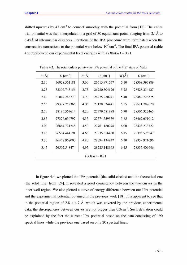
Chapter 4 Experimental results for the NaLi molecule
- 57 -
shifted upwards by 47 cm-1 to connect smoothly with the potential from [18]. The entire
trial potential was then interpolated in a grid of 30 equidistant-points ranging from 2.1Å to
6.45Å of internuclear distances. Iterations of the IPA procedure were terminated when the
consecutive corrections to the potential were below 10-5cm-1. The final IPA potential (table
4.2) reproduced our experimental level energies with a DRMSD = 0.21.
Table 4.2. The rotationless point-wise IPA potential of the 41Σ+ state of NaLi.
R [Ǻ] U [cm-1] R [Ǻ] U [cm-1] R [Ǻ] U [cm-1]
2.10 36028.361181 3.60 26613.971557 5.10 28368.393889
2.25 33307.743156 3.75 26780.504126 5.25 28428.234127
2.40 31049.246273 3.90 26975.230241 5.40 28482.726575
2.55 29377.252365 4.05 27178.334441 5.55 28511.787670
2.70 28186.567614 4.20 27379.581888 5.70 28506.322465
2.85 27376.650797 4.35 27574.539359 5.85 28462.651012
3.00 26864.721248 4.50 27761.180278 6.00 28428.233722
3.15 26584.444191 4.65 27935.656450 6.15 28395.525247
3.30 26478.968000 4.80 28094.134947 6.30 28359.921696
3.45 26502.548474 4.95 28225.148963 6.45 28335.409946
DRMSD = 0.21
In figure 4.4, we plotted the IPA potential (the solid circles) and the theoretical one
(the solid line) from [24]. It revealed a good consistency between the two curves in the
inner well region. We also plotted a curve of energy difference between our IPA potential
and the experimental potential obtained in the previous work [18]. It is apparent to see that
in the potential region of 2.8 ÷ 4.7 Å, which was covered by the previous experimental
data, the discrepancies between curves are not bigger then 0.3cm-1. Such deviation could
be explained by the fact the current IPA potential based on the data consisting of 190
spectral lines while the previous one based on only 20 spectral lines.
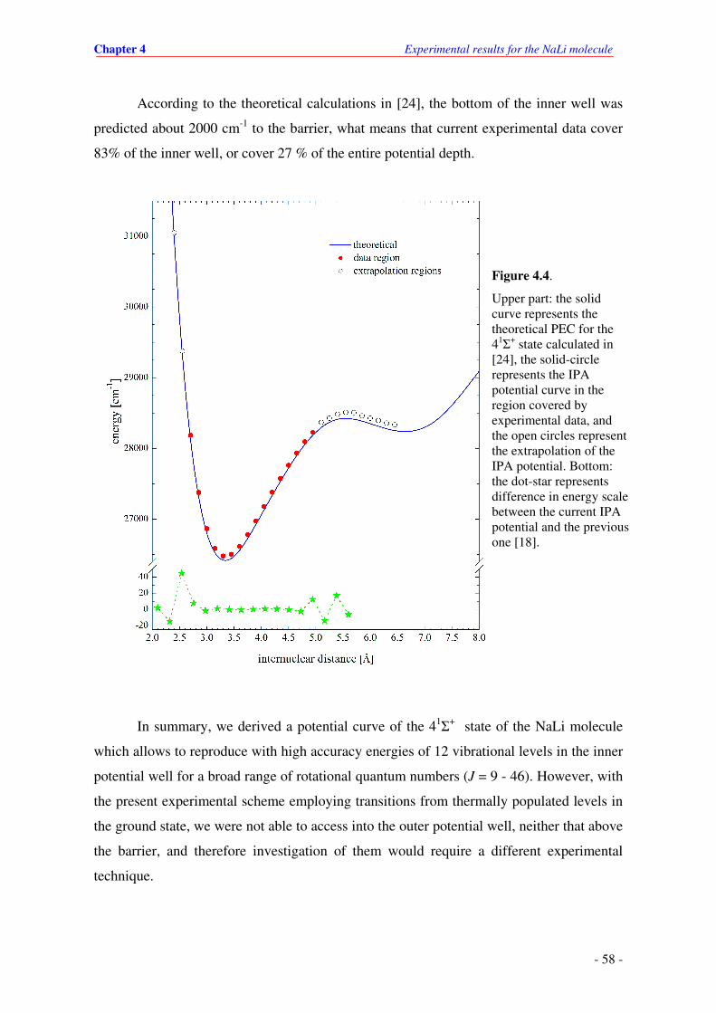
Chapter 4 Experimental results for the NaLi molecule
- 58 -
Figure 4.4.
Upper part: the solid curve represents the theoretical PEC for the 41Σ
+ state calculated in [24], the solid-circle represents the IPA potential curve in the region covered by experimental data, and the open circles represent the extrapolation of the IPA potential. Bottom: the dot-star represents difference in energy scale between the current IPA potential and the previous one [18].
According to the theoretical calculations in [24], the bottom of the inner well was
predicted about 2000 cm-1 to the barrier, what means that current experimental data cover
83% of the inner well, or cover 27 % of the entire potential depth.
In summary, we derived a potential curve of the 41Σ
+ state of the NaLi molecule
which allows to reproduce with high accuracy energies of 12 vibrational levels in the inner
potential well for a broad range of rotational quantum numbers (J = 9 - 46). However, with
the present experimental scheme employing transitions from thermally populated levels in
the ground state, we were not able to access into the outer potential well, neither that above
the barrier, and therefore investigation of them would require a different experimental
technique.
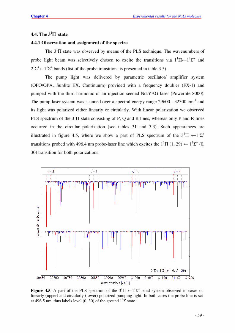
Chapter 4 Experimental results for the NaLi molecule
- 59 -
4.4. The 31ΠΠΠΠ state
4.4.1 Observation and assignment of the spectra
The 31Π state was observed by means of the PLS technique. The wavenumbers of
probe light beam was selectively chosen to excite the transitions via 11Π←11Σ+ and
21Σ+←11Σ+ bands (list of the probe transitions is presented in table 3.5).
The pump light was delivered by parametric oscillator/ amplifier system
(OPO/OPA, Sunlite EX, Continuum) provided with a frequency doubler (FX-1) and
pumped with the third harmonic of an injection seeded Nd:YAG laser (Powerlite 8000).
The pump laser system was scanned over a spectral energy range 29600 - 32300 cm-1 and
its light was polarized either linearly or circularly. With linear polarization we observed
PLS spectrum of the 31Π state consisting of P, Q and R lines, whereas only P and R lines
occurred in the circular polarization (see tables 31 and 3.3). Such appearances are
illustrated in figure 4.5, where we show a part of PLS spectrum of the 31Π ←11Σ+
transitions probed with 496.4 nm probe-laser line which excites the 11Π (1, 29) ← 11Σ+ (0,
30) transition for both polarizations.
Figure 4.5. A part of the PLS spectrum of the 31Π ←11Σ+ band system observed in cases of linearly (upper) and circularly (lower) polarized pumping light. In both cases the probe line is set at 496.5 nm, thus labels level (0, 30) of the ground 11Σ state.

Chapter 4 Experimental results for the NaLi molecule
- 60 -
The rotational quantum numbers of the observed spectral lines can be determined
by taking in to account selection rules (2.71) for change of rotational quantum number.
Assignment of vibrational quantum number was more complicated. Particularly
identification of lines terminating at v = 0 level in the upper state was necessary in order to
assign vibrational quantum numbers to all observed levels in that state. Initially, we
assumed that the lowest observed levels was v = 0. This assignment was confirmed at a
later stage of the analysis by comparison of the Franck–Condon factors with the observed
relative intensities of spectral lines in the following way.
The wavenumbers of these pre-assigned spectral lines were fitted to the relation:
' ' ' " " " ' '( , ) ( , ) ( , )v T v J T v J T v J= − + ∆ . (4.7)
Here, the ' '( , )T v J∆ -term describes the Λ-doubling in the 31Π state, which is given by
' ' 12
1 0
( , ) ( ) [ ( 1) 1]k l
kl
k l
T v J q v J Jδ= =
∆ = + + −
∑∑ , (4.8)
where δ = 0 for f-levels which give rise to Q lines and δ = 1 for e-levels which give rise to
P and R lines. The spectroscopic term values in (4.7) are determined with the Dunham
expansion:
12( , ) ( ) [ ( 1) 1]k l
e kl
k l
T v J T Y v J J= + + + −∑∑ . (4.9)
The obtained Dunham coefficients were used to build an RKR potential and then to
calculate the Franck-Condon (FC) factors for these transitions. In the next step we
compared the envelope-function of the calculated FC factors with the corresponding
intensity distribution of vibrational transitions. Such comparison allowed us to check the
correctness of the pre-assignment of vibrational quantum numbers. In figure 4.6, we
showed a comparison between the observed intensity distribution and the corresponding
FC factors (and its envelope function) in the case of labelled (1, 25) level. In this case
envelope function has a node at v’= 4 for which spectral lines were not observed what
confirms v –assignment.

Chapter 4 Experimental results for the NaLi molecule
- 61 -
Figure 4.7. Distribution of the experimental data in the field of rotational and vibrational quantum numbers of the 31
Π state in NaLi.
Figure 4.6. The envelope function (dashed) of the square of the calculated FCFs (grey bar) and intensity distribution of the observed spectral lines when labelling level was (1, 25).
Once the assignment of the quantum numbers for the chosen progression had been
established the preliminary Dunham coefficients were used to find spectral lines of other
vibrational progressions. Finally we identified 10 vibrational progressions consisting of
380 transitions in the 31Π ← 11Σ+ band system. Distribution of the experimental data in the
field of the rotational and vibrational quantum numbers in the 31Π is plotted in figure 4.7.
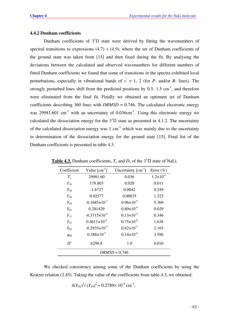
Chapter 4 Experimental results for the NaLi molecule
- 62 -
4.4.2 Dunham coefficients
Dunham coefficients of 31П state were derived by fitting the wavenumbers of
spectral transitions to expressions (4.7) ÷ (4.9), where the set of Dunham coefficients of
the ground state was taken from [15] and then fixed during the fit. By analysing the
deviations between the calculated and observed wavenumbers for different numbers of
fitted Dunham coefficients we found that some of transitions in the spectra exhibited local
perturbations, especially in vibrational bands of v' = 1, 2 (for P- and/or R- lines). The
strongly perturbed lines shift from the predicted positions by 0.3- 1.5 cm-1, and therefore
were eliminated from the final fit. Finally we obtained an optimum set of Dunham
coefficients describing 360 lines with DRMSD = 0.746. The calculated electronic energy
was 29981.601 cm-1 with an uncertainty of 0.036cm-1. Using this electronic energy we
calculated the dissociation energy for the 31П state as presented in 4.1.2. The uncertainty
of the calculated dissociation energy was 1 cm-1 which was mainly due to the uncertainty
in determination of the dissociation energy for the ground state [15]. Final list of the
Dunham coefficients is presented in table 4.3.
Table 4.3. Dunham coefficients, Te and De of the 31Π state of NaLi.
Coefficient Value [cm-1] Uncertainty [cm-1] Error (%)
Te 29981.60 0.036 1.2×10⁻⁴
Y10 178.803 0.020 0.011
Y20 -1.6727 0.0042 0.249
Y30 0.02577 0.00035 1.325
Y40 -0.1685×10⁻³ 0.96×10⁻⁵ 5.369
Y01 0.281429 0.80×10⁻⁴ 0.029
Y11 -0.3715×10⁻² 0.13×10⁻⁴ 0.346
Y21 0.4611×10⁻⁴ 0.75×10⁻⁶ 1.638
Y02 -0.2935×10⁻⁵ 0.62×10⁻⁷ 2.165
q01 0.388×10⁻³ 0.14×10⁻⁴ 3.586
De 6296.8 1.0 0.016
DRMSD = 0.746
We checked consistency among some of the Dunham coefficients by using the
Kratzer relation (2.45). Taking the value of the coefficients from table 4.3, we obtained:
4(Y01)3/ (Y10)
2 ≈ 0.2789× 10⁻⁵ cm-1,

Chapter 4 Experimental results for the NaLi molecule
- 63 -
what is close (within 5%) to Y02 and means that potential curve of 31Π state has regular,
close to Morse function shape (in the experimentally determined range of PEC).
Having precise value of the coefficient describing Λ-doubling (q01) we can try
(with some approximation) to check if it is possible to determine term energy of the state
responsible for Λ-doubling. Assuming Van Vleck’s pure precession model [77] and the
unique perturbation approximation [78], and assuming that Λ-doubling strength in the 13 Π
state is contributed mainly from the coupling between levels of the 13 Π and 16 +Σ states
we can write for the Λ-doubling coefficient following formula:
1
2
013 6
2 ( 1)B l lq
E Eπ +Σ
+≈
−, (4.10)
where B is rotational constant of the 13 Π state, l is angular quantum number of the valence
electron in the atomic state which correlates to both molecular states. Taking into account
B = Y01, q01, 11
3[3 ]eE T
Π= Π (from Tab. 4.3), l = 2 we obtained electronic energy 1[6 ]eT
+Σ
= 27359 cm-1. This value is definitely too low compared with the predicted 29313 cm-1 [24]
what shows that the assumed approximations is inadequate. In fact, the Van Vleck’s pure
precession approximation of the Λ-doubling requires several approximations [61] like :
unique perturber, identical shape of potential curves, each state described by a single
configuration which are weakly fulfilled in case of the 13 Π state: e.g. the potential shape
of the perturbing state ( 16 +Σ ) has not the same shape [24]. Therefore, more sophisticated
treatment is needed in order to explain the value of lambda-doubling coefficient
determined experimentally for the 13 Π .
4.4.3 Potential energy curve
RKR potential
In order to construct potential energy curve of the 13 Π state, first we employed the
semi-classical RKR method. The molecular constants from table 4.3 were used to generate
G(v) and B(v) functions ((2.30) and (2.32)). Pairs of turning points were then calculated
from (2.51a) and (2.51b). Finally we obtained an RKR potential determined with 18 pairs
of the turning points and having a bottom at Re ≅ 3.338 Å. The turning points range from
2.5499 to 5.0118 Å and are listed in table 4.4.

Chapter 4 Experimental results for the NaLi molecule
- 64 -
In the next step we tested accuracy of the RKR potential by comparing the term
values of the observed spectral lines to corresponding eigenvalues obtained by numerical
solving the following RSE (with RKR potential U(R) from tab.4.4):
2 2 2
012 2 [ ( 1) 1] ( ) [ ( 1) 1] ( ) ( )2 2
dJ J U R q J J R E R
dR Rδ χ χ
µ µ
−+ + − + + + − =
. (4.11)
Since the comparison revealed deviations whose magnitude was typically ± 0.9 cm-1 (is far
beyond our experimental uncertainty), therefore we used the IPA method to construct a
more reliable potential for this state.
Table 4.4. The RKR potential energy curve of the 13 Π state of NaLi.
v G(v) [cm-1] R1 [Å] R2[Å]
- 0.49992376(*) 0.000 3.3381392 (Re)
0 88.973 3.1627491 3.5387561
1 264.513 3.0479296 3.7041971
2 436.935 2.9746980 3.8282442
3 606.385 2.9183373 3.9355783
4 773.006 2.8717266 4.0332828
5 936.937 2.8316347 4.1245502
6 1098.311 2.7962768 4.2111259
7 1257.258 2.7645463 4.2940758
8 1413.907 2.7357025 4.3740992
9 1568.378 2.7092215 4.4516785
10 1720.790 2.6847167 4.5271580
11 1871.256 2.6618931 4.6007906
12 2019.889 2.6405193 4.6727656
13 2166.792 2.6204095 4.7432268
14 2312.069 2.6014117 4.8122851
15 2455.817 2.5833991 4.8800265
16 2598.131 2.5662642 4.9465187
17 2739.099 2.5499149 5.0118153
* this row corresponds to bottom of the RKR potential
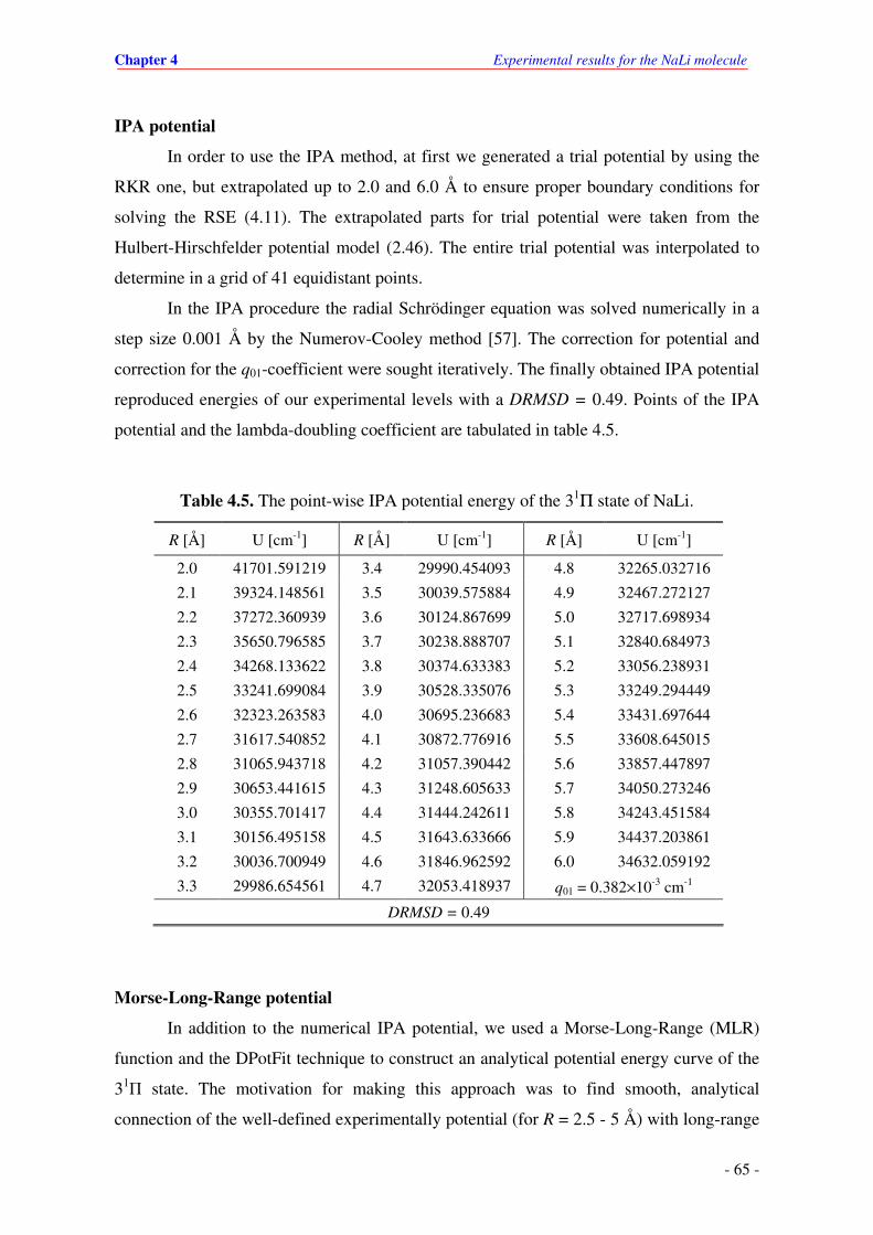
Chapter 4 Experimental results for the NaLi molecule
- 65 -
IPA potential
In order to use the IPA method, at first we generated a trial potential by using the
RKR one, but extrapolated up to 2.0 and 6.0 Å to ensure proper boundary conditions for
solving the RSE (4.11). The extrapolated parts for trial potential were taken from the
Hulbert-Hirschfelder potential model (2.46). The entire trial potential was interpolated to
determine in a grid of 41 equidistant points.
In the IPA procedure the radial Schrödinger equation was solved numerically in a
step size 0.001 Å by the Numerov-Cooley method [57]. The correction for potential and
correction for the q01-coefficient were sought iteratively. The finally obtained IPA potential
reproduced energies of our experimental levels with a DRMSD = 0.49. Points of the IPA
potential and the lambda-doubling coefficient are tabulated in table 4.5.
Table 4.5. The point-wise IPA potential energy of the 31Π state of NaLi.
R [Å] U [cm-1] R [Å] U [cm-1] R [Å] U [cm-1]
2.0 41701.591219 3.4 29990.454093 4.8 32265.032716
2.1 39324.148561 3.5 30039.575884 4.9 32467.272127
2.2 37272.360939 3.6 30124.867699 5.0 32717.698934
2.3 35650.796585 3.7 30238.888707 5.1 32840.684973
2.4 34268.133622 3.8 30374.633383 5.2 33056.238931
2.5 33241.699084 3.9 30528.335076 5.3 33249.294449
2.6 32323.263583 4.0 30695.236683 5.4 33431.697644
2.7 31617.540852 4.1 30872.776916 5.5 33608.645015
2.8 31065.943718 4.2 31057.390442 5.6 33857.447897
2.9 30653.441615 4.3 31248.605633 5.7 34050.273246
3.0 30355.701417 4.4 31444.242611 5.8 34243.451584
3.1 30156.495158 4.5 31643.633666 5.9 34437.203861
3.2 30036.700949 4.6 31846.962592 6.0 34632.059192
3.3 29986.654561 4.7 32053.418937 q01 = 0.382×10⁻³ cm-1
DRMSD = 0.49
Morse-Long-Range potential
In addition to the numerical IPA potential, we used a Morse-Long-Range (MLR)
function and the DPotFit technique to construct an analytical potential energy curve of the
31Π state. The motivation for making this approach was to find smooth, analytical
connection of the well-defined experimentally potential (for R = 2.5 - 5 Å) with long-range

Chapter 4 Experimental results for the NaLi molecule
- 66 -
curve described by (2.53), where Cn coefficients are taken from theory [49]. We expected
that analytical representation of the PEC should be the same as the IPA PEC in the region
of experimental data but also should be able to describe long-range behaviour of the PEC.
As presented in [58], the analytical form of MLR function is represented by:
2
,
,
1 /( ) 1 exp[ ( ). ( , )]
1 /
n m n
m ne eMLR p em n
m n e
RRU R D R y R R
R R
−
−
+ = − −Φ
+
R
R, (4.12)
where yp is the radial expansion variable given by
( , )p p
e
p e p p
e
R Ry R R
R R
−=
+, (4.13)
and
,m nR = Cm/Cn (4.14)
is the ratio between the dispersion coefficients Cm and Cn, and function ( )RΦ is a power
expansion of yp with the set of coefficients φ(k):
0
( ) ( )[ ( , )]NS
k
p e
k
R k y R Rφ=
Φ =∑ for R ≤ Re, (4.15)
0
( ) ( )[ ( , )]NL
k
p e
k
R k y R Rφ=
Φ =∑ for R > Re, (4.16)
where NS and NL are integer numbers to be determined in the DPotFit procedure.
In order to use DPotFit technique, first we generated MLR trial function by fitting
expression (4.12) to the RKR potential from table 4.4. We took value of C6 and C8
coefficients from theoretical calculations [49]. Since the MLR function changes from one
set of p, NS, NL to the other and it was difficult a priori to guess the best one, we
therefore generated the trial MLR function with several combinations of p, NS, NL. For
each combination the DPotFit procedure sought optimum value for the expansion
coefficients φ(k) minimizing deviations between the experimental term values and the
corresponding eigenvalues calculated from the following RSE:
2 2 2
2 2 [ ( 1) 1] ( ) ( ) ( 1) ( ) ( )2 2 MLR
dJ J U R T R J J R E R
dR Rχ χ
µ µ
−+ + − + + ∆ + =
, (4.17)
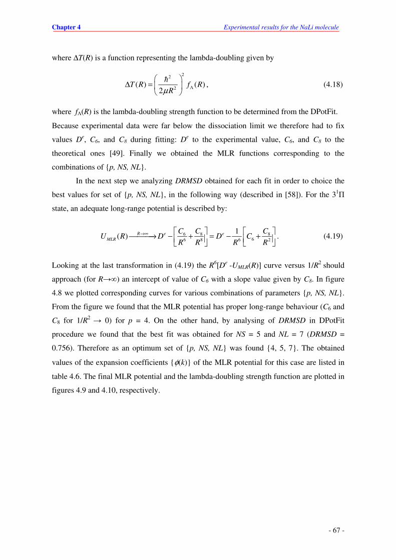
Chapter 4 Experimental results for the NaLi molecule
- 67 -
where ∆T(R) is a function representing the lambda-doubling given by
22
2( ) ( )
2T R f R
RµΛ
∆ =
, (4.18)
where fΛ(R) is the lambda-doubling strength function to be determined from the DPotFit.
Because experimental data were far below the dissociation limit we therefore had to fix
values De, C6, and C8 during fitting: D
e to the experimental value, C6, and C8 to the
theoretical ones [49]. Finally we obtained the MLR functions corresponding to the
combinations of p, NS, NL.
In the next step we analyzing DRMSD obtained for each fit in order to choice the
best values for set of p, NS, NL, in the following way (described in [58]). For the 31Π
state, an adequate long-range potential is described by:
6 8 866 8 6 2
1( ) R e e
MLR
C C CU R D D C
R R R R
→∞ → − + = − +
. (4.19)
Looking at the last transformation in (4.19) the R6[De -UMLR(R)] curve versus 1/R2 should
approach (for R→∞) an intercept of value of C6 with a slope value given by C8. In figure
4.8 we plotted corresponding curves for various combinations of parameters p, NS, NL.
From the figure we found that the MLR potential has proper long-range behaviour (C6 and
C8 for 1/R2 → 0) for p = 4. On the other hand, by analysing of DRMSD in DPotFit
procedure we found that the best fit was obtained for NS = 5 and NL = 7 (DRMSD =
0.756). Therefore as an optimum set of p, NS, NL was found 4, 5, 7. The obtained
values of the expansion coefficients φ(k) of the MLR potential for this case are listed in
table 4.6. The final MLR potential and the lambda-doubling strength function are plotted in
figures 4.9 and 4.10, respectively.

Chapter 4 Experimental results for the NaLi molecule
- 68 -
Figure 4.8. Plot of R6[De-UMLR(R)] function versus 1/R2 for different combinations of
p, NS, NL parameters in the MLR potential function.
Table 4.6. The parameters of MLR 4, 5, 7 potential for the 31Π state of NaLi.
Parameter Value Uncertainty Error (%)
De [cm-1] 6296.72 -------- --------
C6 [cm-1. Å6] 1.5229×10⁸ -------- --------
C8 [cm-1. Å8] 6.2003×10⁹ -------- --------
Re [Å] 3.338943738 1.6×10⁻³ 0.048
φ(0) -2.71837 9.6×10⁻⁴ 0.035
φ(1) 1.225 1.0×10⁻² 0.81
φ(2) 0.151 2.1×10⁻² 13.9
φ(3) 0.955 7.6×10⁻² 7.96
φ(4) 2.25 1.7×10⁻¹ 7.56
φ(5) 2.39 3.6×10⁻¹ 15.06
φ(6) -23.5 1.6 6.8
φ(7) 27.4 1.3 4.74
DRMSD = 0.756

Chapter 4 Experimental results for the NaLi molecule
- 69 -
Figure 4.9. The analytical MLR4, 5, 7 potential of the 31Π state of NaLi (red) and the
difference between the IPA and MLR4, 5, 7 potentials (blue).

Chapter 4 Experimental results for the NaLi molecule
- 70 -
Since last theoretical calculations [79] (which appeared after presented analysis was
done) predict irregular shape of the curve around R = 6.3 Å, so described below analytical
potential is definitely not applicable in the intermediate range of R (around anti-crossing
point). So we would rather consider this situation as a pronounced example that we can not
infer about the shape of PEC outside the region well-represented with the experimental
data.
Finally we compared the MLR potential with the IPA PEC. The comparison
showed that in the region covered by experimental data the agreement between two curves
is better than 0.1 cm-1 (see fig 4.9). Therefore one can conclude that thought both potentials
were constructed in different ways, nevertheless were able to reproduce experimental data
within the experimental uncertainty. Analytical MLR PEC has the long-range part
consistent with assumed expansion coefficients, however it should be greatly stressed that
in the range around anti-crossing point MLR PEC has not physical meaning.
Figure 4.10. Lambda-doubling strength function of the 31Π state.

Chapter 4 Experimental results for the NaLi molecule
- 71 -
4.5. The 41ΠΠΠΠ state
4.5.1 Observation and assignment of the spectra
Spectra of the 41Π state were observed in spectral range 30700 - 33900 cm-1 with
various labelled levels presented in table 3.5. In our experiments, polarization of the pump
light was set linearly in order to enrich experimental data (occurrence of Q branches
together with P and R ones). In figure 4.11, we show a part of polarization spectrum
observed in case of 496.5 nm probe laser line, which labels level (0, 30) in the ground
state.
In total we observed 12 vibrational progressions consisting of 418 spectral lines.
Vibrational quantum numbers for these progressions were determined by comparison
between the relative intensity distribution of spectral lines and the calculated FC factors, in
a similar way as was done before for the 31Π state. We finally identified the quantum
numbers of all spectral lines, ranging in v' = 0 - 19 and J
' = 9 - 57. Distribution of the
experimental data in the field of rotational and vibrational quantum numbers of the 41Π
state is shown in figure 4.12.
Figure 4.11. A part of PLS spectrum consists of P-, Q-, and R-lines of the 41Π ←11Σ+ band in
NaLi, observed for linearly polarized pump beam. The 496.5 nm probe laser line was used.

Chapter 4 Experimental results for the NaLi molecule
- 72 -
Figure 4.12.
Distribution of the experimental data in the field of quantum numbers of the 41
Π state in NaLi.
4.5.2 Dunham coefficients
In order to derive molecular constants for the 41Π state, wavenumbers of the
spectral lines were fitted to relation (4.7), where the lambda-doubling and term values were
represented by (4.8) and (4.9), respectively. The set of Dunham coefficients of the ground
state was taken from [15] and fixed during the fit. We finally obtained an optimum set of
Dunham coefficients (listed in table 4.7) with corresponding DRMSD = 0.62. The
electronic energy of the 41Π state was calculated to be 31178.958cm-1.
Table 4.7. Molecular constants of the 41Π state of NaLi.
Coefficient Value [cm-1] Uncertainty [cm-1] Error (%)
Te 31 178.96 0.024
Y10 169.230 0.014 0.008
Y20 -1.1203 0.0029 0.26
Y30 0.767×10⁻² 0.24×10⁻³ 3.13
Y40 - 0.2329×10⁻³ 0.67×10⁻⁵ 2.88
Y01 0.259530 0.27×10⁻⁴ 0.01
Y11 - 0.24824×10⁻² 0.71×10⁻⁵ 0.29
Y21 -0.414×10⁻⁵ 0.39×10⁻⁶ 9.4
Y02 -0.23349×10⁻⁵ 0.55×10⁻⁸ 0.24
q01 0.2433×10⁻³ 0.61×10⁻⁵ 2.51
De 6193.5 Na 2
1/ 2(4 )P
6199.1 Na 23/ 2(4 )P
1.0
1.0
DRMSD = 0.62

Chapter 4 Experimental results for the NaLi molecule
- 73 -
As presented in sect.4.1.2, the 41Π state dissociates to Li(22S) and Na(42P) atomic
states, thus we can determine its dissociation energy by using (4.2a). However because the
Na (42P) atomic state split into two fine structure components (42P1/2 and 42P3/2) spaced
apart by 6 cm-1 and theoretical calculations do not predict which one is correlated to 41Π
therefore we determined the dissociation energy according to these two possible
asymptotes. Both calculated dissociation energies are listed in table 4.7.
The consistency among some of Dunham coefficients was tested with the Kratzer
relation, Y02 = - 4(Y01)3/ (Y10)
2. Taking value of the coefficients from table 4.7 we obtained
4(Y01)3/ (Y10)
2 ≈ -0.24416×10⁻⁵cm –1. This leads to a relative deviation from Y02 of about
4.47% which indicates that the potential is close to regular in the data region. But on the
other hand recent theoretical calculations showed the anti-crossing with 31Π which deform
both PECs, however it occurs outside the region investigated experimentally.
4.5.3 Potential energy curve
RKR potential
In order to construct the potential energy curve for the 41Π state first we used the
RKR technique. We took molecular constants from table 4.7 to generate the expressions
for G(v) and B(v), given by equations (2.30) and (2.32). The pairs of turning points were
then calculated accordingly to (2.51a) and (2.51b). Finally we obtained a RKR potential
determined in range 2.61-5.31 Å of the internuclear distance listed in table 4.8.
In the next step we tested accuracy of the RKR potential by comparing the
experimental level energies with the corresponding eigenvalues obtained by numerical
solving of the RSE (Eq. 4.11) with the RKR potential. The comparison revealed a
discrepancy of about 1 cm-1 which is beyond our experimental uncertainty. We therefore
used the IPA method to construct a more reliable potential curve.

Chapter 4 Experimental results for the NaLi molecule
- 74 -
Table 4.8. The RKR potential of the 41Π state of NaLi.
v G(v) [cm-1] R1 [Å] R2[Å]
-0.49993978(*) 0.000 3.4761171 (Re) 0 84.326 3.2939898 3.6800588 1 251.339 3.1728517 3.8452480 2 416.174 3.0949457 3.9677685 3 578.865 3.0347549 4.0731419 4 739.442 2.9848986 4.1687557 5 897.928 2.9420129 4.2579826 6 1054.343 2.9042295 4.3427024 7 1208.697 2.8703833 4.4240943 8 1360.998 2.8396884 4.5029611 9 1511.247 2.8115845 4.5798832
10 1659.441 2.7856536 4.6553018 11 1805.568 2.7615736 4.7295664 12 1949.614 2.7390884 4.8029639 13 2091.558 2.7179892 4.8757385 14 2231.373 2.6981026 4.9481037 15 2369.027 2.6792810 5.0202523 16 2504.482 2.6613967 5.0923630 17 2637.694 2.6443374 5.1646055 18 2768.615 2.6280026 5.2371446 19 2897.190 2.6123007 5.3101439
IPA potential
For the convenience we chose the RKR potential as the trial one for using IPA
method. However, for having proper boundary conditions when solving the RSE (4.11) in
the IPA procedure we extrapolated the RKR potential on both sides (to 2.1 and 6.3 Å) by
smooth connection with the Hulbert-Hirschfelder potential (2.46). The entire trial potential
curve was then interpolated to determine in grid of 0.1 Å.
After several IPA iterations, corrections for trial potential and lambda-doubling
coefficient q01 were converged then the IPA procedure was completed. The new lambda-
doubling coefficient was found to be 0.2410 × 10⁻³ cm-1 that is slightly different from the
original value 0.2433 ×10⁻³ cm-1. The final IPA potential (table 4.9) reproduced the
experimental level energies with DRMSD = 0.45.
* this row corresponds to bottom of the RKR potential

Chapter 4 Experimental results for the NaLi molecule
- 75 -
Table 4.9. The point-wise IPA potential of the 41Π state of NaLi.
R [Å] U(R) [cm-1] R [Å] U(R) [cm-1] R [Å] U(R) [cm-1]
2.1 41479.882079 3.6 31211.801127 5.1 33700.815601
2.2 39453.853450 3.7 31279.752084 5.2 33880.731090
2.3 37749.738712 3.8 31378.226171 5.3 34057.588397
2.4 36325.097739 3.9 31501.554723 5.4 34235.302805
2.5 35142.788140 4.0 31644.658190 5.5 34404.306938
2.6 34166.886860 4.1 31803.723797 5.6 34567.302164
2.7 33393.761119 4.2 31974.971660 5.7 34724.379844
2.8 32750.793204 4.3 32155.735608 5.8 34875.483484
2.9 32248.845284 4.4 32343.079154 5.9 35020.555048
3.0 31863.316898 4.5 32535.276102 6.0 35159.574616
3.1 31580.185573 4.6 32730.964384 6.1 35292.560809
3.2 31382.107334 4.7 32927.520812 6.2 35419.565278
3.3 31257.080047 4.8 33124.231695 6.3 35540.668040
3.4 31192.828038 4.9 33318.979429
3.5 31180.530195 5.0 33510.649440 q01= 0. 2410 × 10-3 cm-1
DRMSD = 0.45
From analysis of experimental data we found that the current data covered 51% of
potential well depth, which correspond to region 2.61-5.31Å of internuclear distance. The
IPA potential was plotted in figure 4.13, where solid-circles stand for the experimental data
region. It should be noted that the extrapolation points in the IPA potential were just
introduced to ensure proper boundary conditions when solving the RSE in the IPA
procedure.
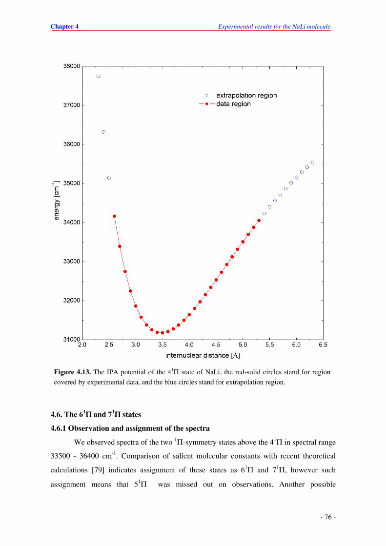
Chapter 4 Experimental results for the NaLi molecule
- 76 -
Figure 4.13. The IPA potential of the 41Π state of NaLi, the red-solid circles stand for region covered by experimental data, and the blue circles stand for extrapolation region.
4.6. The 61ΠΠΠΠ and 7
1ΠΠΠΠ states
4.6.1 Observation and assignment of the spectra
We observed spectra of the two 1Π-symmetry states above the 41Π in spectral range
33500 - 36400 cm-1. Comparison of salient molecular constants with recent theoretical
calculations [79] indicates assignment of these states as 61Π and 71Π, however such
assignment means that 51Π was missed out on observations. Another possible
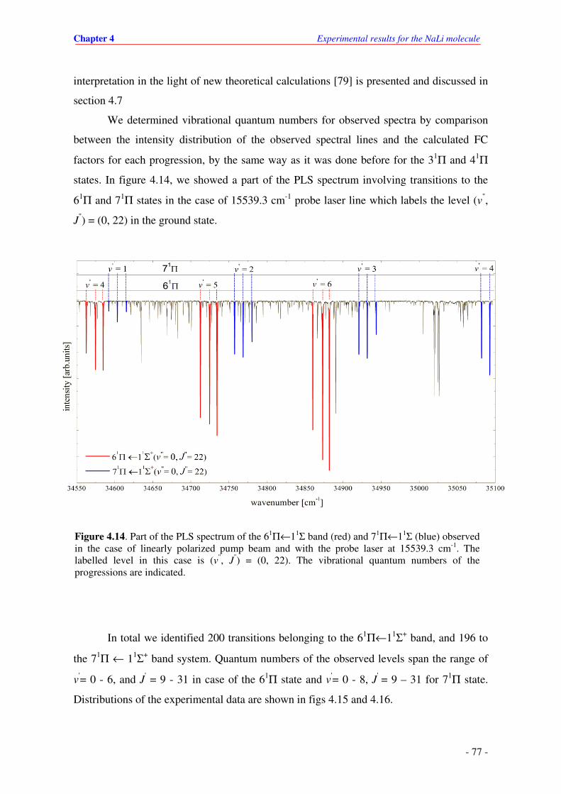
Chapter 4 Experimental results for the NaLi molecule
- 77 -
Figure 4.14. Part of the PLS spectrum of the 61Π←11Σ band (red) and 71Π←11Σ (blue) observed in the case of linearly polarized pump beam and with the probe laser at 15539.3 cm-1. The labelled level in this case is (v", J
") = (0, 22). The vibrational quantum numbers of the progressions are indicated.
interpretation in the light of new theoretical calculations [79] is presented and discussed in
section 4.7
We determined vibrational quantum numbers for observed spectra by comparison
between the intensity distribution of the observed spectral lines and the calculated FC
factors for each progression, by the same way as it was done before for the 31Π and 41Π
states. In figure 4.14, we showed a part of the PLS spectrum involving transitions to the
61Π and 71Π states in the case of 15539.3 cm-1 probe laser line which labels the level (v",
J") = (0, 22) in the ground state.
In total we identified 200 transitions belonging to the 61Π←11Σ+ band, and 196 to
the 71Π ← 11Σ+ band system. Quantum numbers of the observed levels span the range of
v'= 0 - 6, and J' = 9 - 31 in case of the 61Π state and v'= 0 - 8, J' = 9 – 31 for 71Π state.
Distributions of the experimental data are shown in figs 4.15 and 4.16.
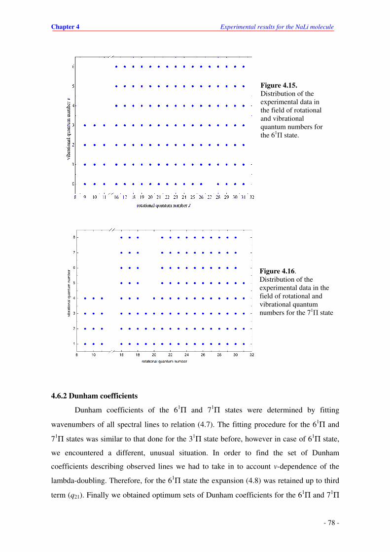
Chapter 4 Experimental results for the NaLi molecule
- 78 -
Figure 4.15. Distribution of the experimental data in the field of rotational and vibrational quantum numbers for the 61
Π state.
4.6.2 Dunham coefficients
Dunham coefficients of the 61Π and 71Π states were determined by fitting
wavenumbers of all spectral lines to relation (4.7). The fitting procedure for the 61Π and
71Π states was similar to that done for the 31Π state before, however in case of 61Π state,
we encountered a different, unusual situation. In order to find the set of Dunham
coefficients describing observed lines we had to take in to account v-dependence of the
lambda-doubling. Therefore, for the 61Π state the expansion (4.8) was retained up to third
term (q21). Finally we obtained optimum sets of Dunham coefficients for the 61Π and 71Π
Figure 4.16. Distribution of the experimental data in the field of rotational and vibrational quantum numbers for the 71
Π state

Chapter 4 Experimental results for the NaLi molecule
- 79 -
states, tabulated in 4.10. The determined values for dissociation energies of the 61Π and
71Π states have the uncertainty of 1 cm-1 due to the uncertainty in determination of the
dissociation energy for the ground state [15].
Table 4.10. Molecular constants of the 61Π and 71Π states of NaLi.
4.6.3 Potential energy curves
RKR potentials
The RKR method was used to construct potential curves for the 61Π and 71Π. First
we used molecular constants from table 4.10 to generate the vibrational and rotational
functions (relations (2.30) and (2.32)), and then calculated turning points by integration of
(2.51a) and (2.51b). Finally we obtained RKR potentials for the 61Π and 71Π states. The
RKR potential of the 61Π state was determined in seven pairs of turning points ranging
from 2.85 to 4.32 Å. The RKR for the 71Π state was determined in eight pairs of turning
points ranging from 2.82 to 4.48 Å. Details of these RKR potentials are listed in table 4.11.
In next step we tested accuracy of the RKR potentials by comparing experimental
level energies to the corresponding eigenvalues of the following RSE (with the RKR
potentials):
61Π state 71Π state Coefficient
Value Uncertainty Error (%)
Value Uncertainty Error (%)
Te [cm-1] 34042.28 0.04 9×10⁻⁵ 34535.82 0.037 0.0
De [cm-1] 4346 1.0 2.3×10⁻⁴ 4429 1.0 2.2×10⁻⁴
Y10 [cm-1] 168.990 0.03 0.018 170.497 0.024 0.014
Y20 [cm-1] -2.2559 0.0084 37 -0.9399 0.58×10⁻² 0.62
Y30 [cm-1] 0.7397×10⁻¹ 0.76×10⁻³ 0.1 -0.1285×10⁻¹ 0.42×10⁻³ 3.29
Y01 [cm-1] 0.27163 0.00011 0.04 0 .2634501 0.917×10⁻⁴ 0.035
Y11 [cm-1] -0.4648×10⁻² 0.50×10⁻⁴ 1.07 -0.2722×10⁻² 0.93×10⁻⁵ 0.34
Y21 [cm-1] 0.1165×10⁻³ 0.68×10⁻⁵ 5.8 ------- ------ -------
Y02 [cm-1] -0.2347×10⁻⁵ 0.76×10⁻⁷ 3.2 -0.2492×10⁻⁵ 0.8×10⁻⁷ 3.2
q01 [cm-1] -0.5972×10⁻² 0.58×10⁻⁴ 0.97 -0.24122 ×10⁻³ 0.164×10⁻⁴ 6.82
q11 [cm-1] 0.2107×10⁻² 0.36×10⁻⁴ 1.7 ------- -------- ------
q21 [cm-1] -0.2888×10⁻³ 0.48×10⁻⁵ 1.66 ------- -------- ------
DRMSD = 0.56 DRMSD = 0.66

Chapter 4 Experimental results for the NaLi molecule
- 80 -
2 2 21
1 22 20
[ ( 1) 1] ( ) ( ) [ ( 1)]2 2
k
k
k
dJ J U R q v J J E
dR Rδ χ χ
µ µ =
−+ + − + + + + =
∑
. (4.21)
In (4.21) δ = 0 for f-parity levels, δ = 1 for e-parity levels, k = 0 for the 71Π state, and k =
0, 1 and 2 for the 61Π. Our comparison revealed deviations are of about 1.7 cm-1 for the
61Π state, and 0.7 cm-1 for the 71
Π state. Such deviations were too large; therefore we used
the IPA technique to construct more confident potentials which are capable of representing
the data within the experimental uncertainty.
Table 4.11. The RKR potentials of the 61Π and 71Π states of NaLi.
61Π 71Π
v G(v)/cm-1 R1 [Å] R2[Å] v G(v)/cm-1
R1 [Å] R2[Å]
-0.49976 0.000 3.3978289 (Re) -0.500349 0.000 3.4501610 (Re)
0 83.899 3.2193073 3.6066316 0 85.072 3.2691518 3.6537746
1 248.617 3.1041591 3.7821414 1 253.647 3.1496179 3.8188589
2 409.489 3.0312572 3.9150026 2 420.228 3.0731104 3.9414105
3 566.959 2.9753835 4.0302608 3 584.735 3.0141592 4.0469361
4 721.471 2.9293466 4.1349217 4 747.093 2.9653751 4.1428632
5 873.468 2.8899259 4.2320092 5 907.223 2.9233806 4.2326103
6 1023.394 2.8553708 4.3230687 6 1065.050 2.8862944 4.3181020
7 1220.495 2.8529395 4.4005614
8 1373.482 2.8225199 4.4808338
IPA potentials
In the IPA method we used the RKR potential but extrapolated on both sides up to
2.3 and 5.2 Å for the 61Π state, and up to 2.2 and 5.7Å for the 71
Π as the trial ones. The
extrapolations were performed with Hulbert-Hirschfelder potential (2.46) connected
smoothly with the RKR potentials. Each potential was then interpolated in grid of 0.1Å.
In the IPA procedure lambda-doubling coefficients q01 were fitted in the case of
both states whereas the values of the coefficients q11 and q21 for v-dependent lambda-
doubling in the 61Π state were fixed to the value obtained from former analysis. The final
IPA potentials could reproduce the experimental level energies with DRMSD = 0.53 for the

Chapter 4 Experimental results for the NaLi molecule
- 81 -
61Π state and with DRMSD = 0.45 for the 71
Π state. Details of these potentials are
tabulated in tables 4.12 and 4.13.
Table 4.12. The point-wise IPA potential of the 61Π state of NaLi.
R [Å] U(R) [cm-1] R [Å] U(R) [cm-1] R [Å] U(R) [cm-1]
2.3 40133.328902 3.4 34041.025103 4.5 35425.358757
2.4 38745.026620 3.5 34066.083430 4.6 35621.494849
2.5 37597.801196 3.6 34120.704594 4.7 35820.960096
2.6 36668.069206 3.7 34209.911801 4.8 36022.172710
2.7 35925.441133 3.8 34310.312763 4.9 36222.916609
2.8 35345.978618 3.9 34440.336109 5.0 36420.638447
2.9 34868.939503 4.0 34561.265147 5.1 36612.613058
3.0 34522.519597 4.1 34730.338976 5.2 36796.448900
3.1 34297.894253 4.2 34848.356054 q01 = -0.5907×10⁻²
3.2 34142.629495 4.3 35044.324286 q11 = 0.2107×10⁻²
3.3 34066.872671 4.4 35232.582679 q21 = -0.2888×10⁻³
DRMSD = 0.53
Table 4.13. The point-wise IPA potential of the 71Π state of NaLi.
R [Å] U(R) [cm-1] R [Å] U(R) [cm-1] R [Å] U(R) [cm-1]
2.2 42773.090325 3.4 34542.432452 4.6 36138.867581
2.3 41050.412540 3.5 34541.055600 4.7 36335.564236
2.4 39618.450139 3.6 34582.265169 4.8 36528.672430
2.5 38426.894848 3.7 34658.558468 4.9 36718.513403
2.6 37451.543624 3.8 34764.033784 5.0 36888.187407
2.7 36662.392797 3.9 34893.875295 5.1 37048.964080
2.8 36043.749063 4.0 35042.462253 5.2 37200.853216
2.9 35549.534313 4.1 35206.256394 5.3 37343.888479
3.0 35170.186560 4.2 35381.409116 5.4 37480.373940
3.1 34896.980240 4.3 35564.799307 5.5 37610.396550
3.2 34709.360994 4.4 35752.232486 5.6 37733.503810
3.3 34595.872514 4.5 35939.528873 5.7 37849.243210
q01= 0.240242×10⁻³ cm-1
DRMSD = 0.45
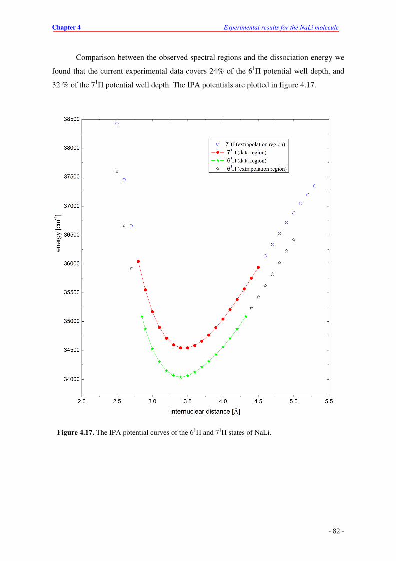
Chapter 4 Experimental results for the NaLi molecule
- 82 -
Figure 4.17. The IPA potential curves of the 61П and 71
П states of NaLi.
Comparison between the observed spectral regions and the dissociation energy we
found that the current experimental data covers 24% of the 61Π potential well depth, and
32 % of the 71Π potential well depth. The IPA potentials are plotted in figure 4.17.

Chapter 4 Experimental results for the NaLi molecule
- 83 -
4.7. Comparison of the current results with recent theoretical calculations
Soon after our experimental observations for the 71Π state, two independent
theoretical papers with comprehensive study on electronic structure of NaLi appeared in
2008 [79, 80]. In both theoretical works the electronic structure of NaLi molecule was
explored up to the Na (32P) - Li (22P) atomic asymptote, which correlates among others to
the 71Π state. The authors calculated important molecular constants (listed in table 4.14)
and potential curve for each electronic state. The calculated values of molecular constants
in both papers are slightly different for the low-lying states below the Na(32S)-Li(32P)
asymptote. However, deviations between the two theoretical results increase for higher
excited states, particular for the 71Π state. Considering the values of electronic energy (Te)
and dissociation energy (De) of the 71Π obtained in [79] and [80], we find following energy
differences between two results: 1615 cm-1 for Te, and 1966 cm-1 for De. Obviously such
differences for Te and De are not acceptable and they exceed acceptable inaccuracy, and
therefore one can point out the more correct (closer to experimental) theoretical
calculations are necessary. Presently, having experimental results it is possible to check
reliability of the two theoretical results by comparing them to the experimental ones. In
table 4.14 we list the theoretical and experimental values of molecular constants for the
41Σ+, 31Π, 41
Π, 61Π and 71
Π states.
Table 4.14. Theoretical and experimental molecular constants for the 41∑+, 31Π, 41
Π, 61Π and 71
Π
states of NaLi.
Molecular constant 41Σ+ 31
Π 41Π 61
Π 71Π Reference
Te [cm-1] 26474.19 26457 26184
29981.60 29992 29900
31178.96 31155 30904
34042.28 34027 34338
34535.82 34541 36156
this work [79] - theory [80] - theory
ωe [cm-1] 179.673 181.86
178.804 176.74
169.325 170.33
168.990 167.74
170.497 171.35
this work [79] - theory
Re [Å] 3.3430
3.328 3.387
3.3358 3.344 3.392
3.4710 3.460 3.493
3.3978 3.397 3.477
3.4502 3.444 3.746
this work [79] - theory [80] - theory
De [cm-1]
6370 6340 5888
6297 6236 6130
6193 6171 5646
4346 4321 4194
4429 4386 2420
this work [79] - theory [80] - theory
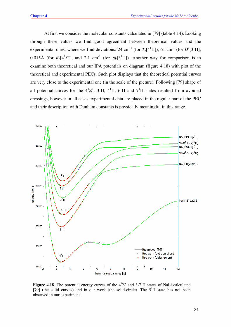
Chapter 4 Experimental results for the NaLi molecule
- 84 -
Figure 4.18. The potential energy curves of the 41Σ+ and 3-71Π states of NaLi calculated
[79] (the solid curves) and in our work (the solid-circle). The 51Π state has not been
observed in our experiment.
At first we consider the molecular constants calculated in [79] (table 4.14). Looking
through these values we find good agreement between theoretical values and the
experimental ones, where we find deviations: 24 cm-1 (for Te[41Π]), 61 cm-1 (for De[31
Π],
0.015Å (for Re[41Σ+], and 2.1 cm-1 (for ωe[3
1Π]). Another way for comparison is to
examine both theoretical and our IPA potentials on diagram (figure 4.18) with plot of the
theoretical and experimental PECs. Such plot displays that the theoretical potential curves
are very close to the experimental one (in the scale of the picture). Following [79] shape of
all potential curves for the 41Σ+, 31Π, 41
Π, 61Π and 71
Π states resulted from avoided
crossings, however in all cases experimental data are placed in the regular part of the PEC
and their description with Dunham constants is physically meaningful in this range.

Chapter 4 Experimental results for the NaLi molecule
- 85 -
The relative good agreement with the experimental results indicates the theoretical
calculations for NaLi in [79] are quite reliable. However, there appears a problem due to
missing of 51Π from experimental observation. At the moment there is not any reasonable
explanation for this but it seems that this is not an experimental fault or oversight.
Recorded spectra in region that we expected to observe spectrum of the 51Π were of very
good quality (S/N ratio), all registered progressions were assigned to 41Π and 61
Π states, or
to Na2 spectrum which was precisely known from former measurements [30]. There were
no any evidences of lines to the 51Π state. One can not expect unusually small transition
dipole moment of the 51Π ← 11Σ+ band system; however there is not actually calculation
of it. We would lean towards the suspicion that theoretical calculations are not correct for
this state. On the other hand we see that this is somehow in contradiction with very good
agreement for other states.
When turning to the comparison between theoretical values calculated in [80] and
the experimental ones we see from table 4.14 that agreement between the theoretical and
the experimental values is not good, much worse then that were for [79]. Indeed, for the
71Π state we find huge deviations of 1620 cm-1 for Te and 0.296 Å for the equilibrium
internuclear distance (Re). But if for the moment we would allow for a such big
discrepancy one can see from fig. 4.19 that another assignment of the two highest states is
possible, namely as 51Π and 61
Π. This would solve the problem of missing 51Π state, but
would show up big inaccuracy of calculations, e.g. deviations for Te and Re in these states
(with new 5-61Π-assignment) would be: 198 cm-1 for Te [61
Π], 250 cm-1 for Te [51Π],
0.0268 Å for Re [61Π], and 0.1792 Å for Re [5
1Π]. The last value of deviation for Re is quite
big compared to those for other states, and it is well above that expected from nowadays
theoretical calculations for alkali dimers. At the moment, from the experimental side nothing more can be done. We hope
that this intriguing situation will be explained with the help of theoreticians when they get
our (still not published) results for the highest states. Looking at the comparison of all data
in tab.4.14 and potential curves in figs. 4.18 ÷ 4.20 we would incline that the theoretical
calculations in [79] are more reliable than of [80], however this leaves riddle of the 51Π
state unravelled.
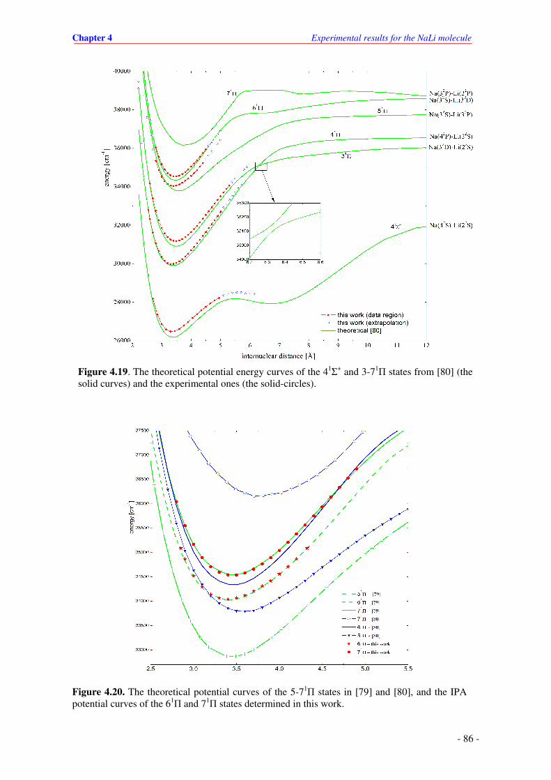
Chapter 4 Experimental results for the NaLi molecule
- 86 -
Figure 4.19. The theoretical potential energy curves of the 41Σ+ and 3-71Π states from [80] (the
solid curves) and the experimental ones (the solid-circles).
Figure 4.20. The theoretical potential curves of the 5-71Π states in [79] and [80], and the IPA
potential curves of the 61Π and 71
Π states determined in this work.

Chapter 5 Summary and conclusions
- 87 -
Chapter 5
Summary and conclusions
Polarization labelling spectroscopy technique has been used to study the
rovibrational structure of several excited electronic states of NaLi. All investigated
electronic states of 1Π-symmetry were unknown (unobserved) before our measurements.
There were also no theoretical calculations for them, until August 2008. Nevertheless, on
the basis of the characteristic features of the observed polarisation spectra we have
identified unambiguously the symmetry of each of these states, and by numerical analysis
we characterised them, obtaining molecular (Dunham) constants and constructed reliable
potential energy curve for each state. Besides the four 1Π-symmetry states, we also
recorded transitions to the previously investigated 41Σ+ state [18] and using the much
richer current data set we could refine the existing description of this state.
Finally in the 26000-36300 cm-1 spectral region we observed five electronic states
accessible directly by optical transitions from the ground state (e.g. singlet states of Σ+-, Π-
symmetry).
The 41Σ+ state was previously investigated by the polarization labelling
spectroscopy technique [18]. In that first experiment (with the Ar+ laser used as a probe
laser) only one progression was registered and molecular constants and a potential energy
curve were determined only from a single vibrational progression. Within the current
experiments we used the tunable dye laser as a probe laser, and could choose several
probing transitions. It turned out that a more precise description of this state was possible
with such complementary data. Finally we observed 200 spectral lines and then converted
them into the molecular constants and to the IPA potential. According to theoretical

Chapter 5 Summary and conclusions
- 88 -
predictions [24, 79-80] the 41Σ+ state has a double-minimum potential well due to avoided
crossing with the 51Σ+ state. Our analysis showed that the presently collected experimental
data cover the inner well of the PEC, which was predicted to be regular. Therefore the
determined molecular constants represent spectroscopic characterization of this regular
part of the PEC, and only this part.
The measured spectra of the 31Π and 41
Π states consisted of 367 and 361 lines,
respectively. Analysis of the spectra revealed the presence of local perturbations affecting
P- and/or R- lines to v = 1, 2 vibrational levels of the 31Π state. According to the
calculations in the recent theoretical paper [79], the potential curves of the 61Σ+ and 31Π
states cross each other at a point near the bottom of the potential curve of the 31Π state.
Therefore, we can expect such local perturbations to be mainly due to non-adiabatic
couplings between the 31Π and 61Σ+ states. By using Dunham expansion we determined
molecular constants for the 31Π and 41
Π states. It turned out that construction of potential
energy curves for the 31Π and 41
Π states by the RKR method yielded important
information (equilibrium internuclear distance, position of vibrational levels), and the RKR
potentials were sufficiently accurate for comparison with theoretical ones. However in
order to obtain PEC that is sufficiently precise to reproduce high resolution data the IPA
technique was used to further refine these potential curves. Having the constructed IPA
potentials we checked, that the experimental data for the 31Π and 41
Π states could be
reproduced to within our experimental uncertainty. Since the dispersion coefficients for the
long-range potential of the 31Π state were calculated theoretically [49], we tried to connect
the long-range potential part of the PEC with the part covered by the experimental data.
This was the motivation for the construction of a Morse-long-range (MLR) potential for
the 31Π state by using the DPotFit technique. However, recent predictions in [79, 80]
(which appeared after this analysis was done) showed that the outer potential wall of the
31Π state is deformed in the region of 6.3 Å due to avoided-crossing with the 41
Π state.
Therefore, in the region around the anti-crossing point we clearly cannot use regular curve
description. The analytical MLR potential presented in this thesis should be considered
only as a mathematical connection between the near-equilibrium part of the potential
(determined by the experimental data) and the long-range part. Although the analytical
MLR PEC has the long-range part consistent with assumed (real) expansion coefficients, it
should be stressed that in the range around the anti-crossing point the MLR PEC has no
physical meaning.

Chapter 5 Summary and conclusions
- 89 -
The 61Π and 71Π states were the highest ones studied in this work. In total, 200
spectral lines for the 61Π state and 196 spectral lines for the 71Π state were identified in the
polarisation spectra. In case of the 61Π state it turned out that strongly v-dependent
lambda-doubling had to be taken into account in order to interpret the experimental data.
The positions of spectral lines were converted to the energies of rovibrational levels in the
61Π and 71Π states and then processed in the same way as described above for the 41Π
state. In this manner the molecular constants and the equilibrium internuclear distance
were determined for each state, and then RKR potential energy curve, with further
refinement with IPA technique was constructed. Finally the constructed IPA potentials for
the 61Π and 71Π reproduced the experimental data within the experimental uncertainty.
Soon after our observations of the highest 1Π state, two papers [79, 80] with
comprehensive theoretical calculations of electronic structure of NaLi appeared (August
2008). For low-lying electronic states, below 41Π, calculated values for molecular
constants in both works are quite close to each other, and also close to those determined
experimentally by us. However deviations between these two theoretical results increase
for higher excited states. Particularly huge discrepancies between the two calculated results
can be found for the 71Π state, where disagreement between the electronic energy is
1615 cm-1, and 0.3Å between the equilibrium internuclear distances. Such deviations are
very big; they exceed what we can expect from the nowadays precise calculations for
alkali-metal dimers. Since both theoretical works considered electronic states up to
Na(32P)-Li(22P) asymptote, which correlates to the 71Π state, we could compare both
theoretical results to our experimental ones, and attempted to assess the reliability of both
theoretical approaches. The comparison shows much better agreement of our data with the
results by Mabrouk et al [79]. For example, if we accept the numbering of the states given
in [79], the deviation of the electronic energy for the 71Π state is only 5 cm-1, and of the
equilibrium distance is 0.006 Å. However an unexpected problem appears: if we keep the
assignment for the 1Π states following [79] this would mean that we missed the 51Π state
in our observations. This is hardly an acceptable explanation because we did a systematic,
careful spectroscopic search thorough the corresponding energy range and it is not
probable that we overlooked a few hundred lines. Since there is no clear reason for a
particularly small transition dipole moment to the 51Π state, this would lead us to the
conclusion that the position of this state is not well calculated in [79], which also means

Chapter 5 Summary and conclusions
- 90 -
that the numbering of the 1Π states is not correct. However, we see some counterargument,
namely that the positions of other states in [79] were predicted very well.
If we compare our results for the 61Π and 71Π states with those in [80] generally
the shift of the positions of PECs is much bigger. But surprisingly, if we accept such
discrepancy, the problem of the missing 51Π state disappears, since another assignment of
the highest experimentally observed states is possible, as 5 and 61Π states. Again, an
argument against such explanation is the generally bad agreement of theoretical and
experimental PECs for both 51Π and 61Π states.
At the present moment we do not have a convincing explanation for inconsistency
between our and theoretical results described above, and also between the two theoretical
calculations. Since from the experimental side nothing more can be done at the moment,
we hope for revisiting of the calculations by theoreticians. Since our last results for the 61Π
and 71Π states are already prepared for publication (until now they have not published in
any form) we believe that this will stimulate theoretical reinvestigation of NaLi electronic
structure.
Bibliography
- 91 -
Bibliography
[1] W. D. Phillips. Laser cooling and trapping of neutral atoms. Rev. Mod. Phys. 70
(1998) 721-741.
[2] J. Weiner, V. S. Bagnato and S. Zilio, P. S. Julienne. Experiments and theory in cold
and ultracold collisions. Rev. Mod. Phys., 71 (1999) 1-85.
[3] Thorsten Köhler, Krzysztof Góral, and Paul S. Julienne. Production of cold molecules
via magnetically tunable Feshbach resonances. Rev. Mod. Phys. 78, (2006) 1311.
[4] V. Wippel, C. Binder, and L. Windholz. Cross-section for collisions of ultracold 7Li
with Na. Eur. Phys. J. D 21 (2002) 101-104.
[5] C. A. Stan, M.W. Zwierlein, C. H. Schunck, S.M. F. Raupach, and W. Ketterle.
Observation of Feshbach Resonances between Two Different Atomic Species. Phys.
Rev. Lett., 93 (2004) 1-4.
[6] G Auböck, C Binder, L Holler, V Wippel, K Rumpf, J Szczepkowski1, W E Ernst and
LWindholz. Trap loss collisions of 6Li and 7Li with 23Na in a combined magneto-
optical trap. J. Phys. B: At. Mol. Opt. Phys. 39 (2006) S871–S879.
[7] W. C. Stwalley and H. Wang. Photoassociation of Ultracold Atoms: A New
Spectroscopic Technique. J. Mol. Spectr., 195 (1999) 194-228.
[8] K. M. Jones, E. Tiesinga, P. D. Lett, and P. S. Julienne. Ultracold photoassociation
spectroscopy: Long-range molecules and atomic scattering. Rev. Mod. Phys. 78
(2006) 435.
[9] J. M. Walter, S. Barrat. The Existence of Intermetallic Compounds in the Vapor State.
The Spectra of the Alkali Metals and their Alloys with Each Other. Proc. R. Soc.
Lond. A 119, 257-275, (1928)

Bibliography
- 92 -
[10] B. B. Phillips, H. M. Froslie, and R. H. McFarland. An Investigation of the Existence
of a Sodium Lithium Molecule. Phys. Rev. 81 (1951) 898 – 899.
[11] M. M. Hessel. Experimental Observation of the NaLi Molecule. Phys. Rev. Lett., 26
(1971) 215-218.
[12] F. Engelke, G. Ennen, and k. H. Meiwes. Laser Induced Fluorescence Spectroscopy of
NaLi in Beam and Bulk. Chem. Phys., 66 (1982) 391-402.
[13] M. M. Kappe, K. O. Marti, P. Radi, M. Schäp, and E. Scgumacher. Resonant two-
photon ionization of LiNa. Observation and preliminary characterization of five new
singlet states. Chem. Phys. Lett.,107 (1984) 6.
[14] C.E. Fellows, J.Vergès, and C. Amiot. The NaLi electronic ground state studied by
laser induced fluorescence and Fourier transform spectroscopy. Mol.
Phys., 63 (1988) 1115.
[15] C.E. Fellows. The NaLi 11Σ+(X) electronic ground-state dissociation limit. J. Chem.
Phys., 94 (1991) 5855-5864.
[16] C.E. Fellows. The NaLi 1(2)A
+Σ electronic state: first high-resolution spectroscopic
study. J. Mol. Spectrosc, 136 (1989) 369-379.
[17] C.E. Fellows, J.Vergès, and C. Amiot. The Na7Li 31Σ+(C) and 11Π(B) electronic
states through collision energy transfer. J. Chem. Phys., 93 (1990) 6281-6290.
[18]. W. Jastrzębski, P. Kowalczyk, R. Nadyak, and A. Pashov. Spectroscopic study of the
41Σ+(E) state in NaLi. Spectrochim. Acta, Part A, 58A (2002) 2193.
[19] P.J. Bertocini, G. Das, and A. C. Wall. Theoretical study of the 1 3 3 1, , ,+ +Σ Σ Π Π
States of NaLi and the 2∑+
state of NaLi+. J. Chem. Phys., 52 (1970) 5112-5130.
[20] S. Green. Electric Dipole Moment of Diatomic Molecules by Configuration
Interaction. I.Closed-Shell Molecules. J. Chem. Phys., 54 (1971) 827-832.
[21] P. Rosmus and W. Meyer. Spectroscopic constants and the dipole moment functions
for the 1∑+
ground state of NaLi. J. Chem. Phys., 65 (1976) 492- 493.
[22] W. Müller, Joachim Flesch, and W. Meyer. Treatment of intershell correlation effects
in ab initio calculations by use of core polarization potentials. Method and

Bibliography
- 93 -
application to alkali and alkaline earth atoms. J. Chem. Phys., 80 (1984) 3297-
3310.
[23] W. Müller and W. Meyer. Ground-state properties of alkali dimers and their cations
(including the elements Li, Na, and K) from ab initio calculations with effective core
polarization potentials. J. Chem. Phys., 80 (1984) 3311-3320.
[24] I. Schmidt-Mink, W. Muller, and W. Meyer. Potential energy curves for ground and
excited states of NaLi from ab initio calculations with effective core polarization
potentials. Chem. Phys. Lett., 112 (1984) 120-129.
[25] P. J. Dagdigian, J. Graff, and L. Warton. Stark effect of NaLi X1Σ+. J. Chem. Phys.,
55 (1971) 4980-4982.
[26] J. Graff, P. J. Dagdigian, and L. Warton. Electric Resonance Spectrum of NaLi. J.
Chem. Phys., 57 (1972) 710-714.
[27] R. Teets, R. Feinberg, T. W. Hansch, and A. L. Schawlow. Simplification of spectra
by Polarization Labelling. Phys. Rev. Lett., 37 (1976) 683.
[28] W. Jastrzebski and P. Kowalczyk. Polarization labelling spectroscopy of 31Πu- X
1Σ
+g
and 31Σ
+u - X
1Σ
+g transitions in K2. Chem. Phys. Lett., 206 (1993) 69.
[29] Pashov, Jastrzebski, and Kowalczyk. The Li2 F1Σ
+g "Shelf state: accurate potential
energy curve based on the inverted perturbation approach. J. Chem. Phys., 113
(2000) 6624.
[30] I. Jackowska et al. Reanalysis of the A Σ+
u state of Na2 by polarization labelling
spectroscopy. Mol. Phys., 89 (1996) 1719.
[31] W. Jastrzebski and P. Kowalczyk. Potential curves for selected electronic states of K2
and NaK. Phys. Rev. A., 55 (1997) 2438.
[32] V. Bednarska, I. Jackowska, W. Jastrzebski, P. Kowalczyk. The Molecular Constants
and Potential Energy Curve of the Ground State X1Σ
+in KLi. J. Mol. Sectrosc., 189
(1998) 244-248.
[33] P. Kortyka, W. Jastrzebski, P. Kowalczyk. Experimental characterisation of the
double minimum 61Σ
+ state in NaRb. Chem. Phys. Lett., 404 (2005) 323-326.
[34] G. Herzberg: Molecular Spectra and Molecular Structure. Vol. 1: Spectra of
Diatomic Molecules. Van Nostrand, 1950.

Bibliography
- 94 -
[35] J. Brown and, A. Carrington: Rotational Spectroscopy of Diatomic Molecules.
Cambridge University Press, 2003.
[36] B. H. Bransden, and C. J. Joachain: Physic of Atoms and Molecules. Longman
Scientific & Technical, 1983.
[37] J. Hirschfelder, C. Curtiss, and R. B. Brird: Molecular Theory of Gases and Liquids,
John Wiley & Sons, 1954.
[38] A. Hinchliffe: Modelling molecular Structure, 2nd. John Wiley, 2000.
[39] Y. P. Varshni. Comparative Study of Potential Energy Functions for Diatomic
Molecules. Rev. Mod. Phys., 29 (1957) 664-682.
[40] G. Calder and K. Ruedenberg. Quantitative Correlations between rotational and
vibrational spectroscopic Constants in Diatomic Molecules. J. Chem. Phys., 49
(1968) 5399-5415.
[41] J. L. Dunham. Diatomic Molecules According to the Wave Mechanics. II. Vibrational
Levels. Phys. Rev., 34 (1929) 57-64.
[42] J. L. Dunham. The Wentzel-Brillouin-Kramers Method of Solving the Wave Equation.
Phys. Rev., 41 (1932) 713-720.
[43] C. Beckel and R. Engelke. Power-Series Expansions of Vibrational Potentials. IV.
Radii of Convergence. J. Chem. Phys., 49 (1968) 5199-5200.
[44] P. Morse. Diatomic Molecules According to the Wave Mechanics. II. Vibrational
Levels. Phys. Rev., 34 (1929) 57.
[45] A. S. Coolidge, H. M. James, and E. L. Vernon. On the Determination of Molecular
Potential Curves from Spectroscopic Data. Phys. Rev. 54 (1938) 726 – 738.
[46] H. Hulbert, and J. Hirschfelder. Potential Energy Functions for Diatomic Molecules.
J. Chem. Phys. 9 (1941) 61-69.
[47] C. L. Pekeris. The Rotation-Vibration Coupling in Diatomic Molecules. Phys. Rev. 45
(1934) 98 -103.
[48] R. Leroy, in: Molecular Spectroscopy, Vol 1, Eds. R. F. Barrow, D. A. Long, and D.
J. Millen (Chem. Soc., London, 1973).

Bibliography
- 95 -
[49] M. Marinescu, and H. R. Sadeghpour. Long-range potentials for two-species alkali-
metal atoms. Phys. Rev. A 59 (1999) 390 – 404.
[50] M. Marinescu and A. Dalgarno. Dispersion forces and long-range electronic
transition dipole moments of alkali-metal dimer excited states. Phys. Rev. A 52
(1995) 311 – 328.
[51] M. Marinescu and Anthony F. Starace. Dispersion coefficients for highly excited
molecular states of K2. Phys. Rev. A 56 (1997) 4321 – 4323.
[52] M. Marinescu. Dispersion coefficients for the nP-nP asymptote of homonuclear
alkali-metal dimmers. Phys. Rev. A 56 (1997) 4764 – 4773.
[53] Bing Ji, Chin- Chun Tsai, and W. Stwalley. Proposed modification of the criterion for
the region of validity of inverse-power expansion in diatomic long-range potentials.
Chem. Phys. Lett. 236 (1995) 242-246.
[54] W.M. Kosman and J. Hinze. Inverse Perturbation Analysis: Improving the Accuracy
of Potential Energy Curves. J. Mol. Spectr., 56 (1975) 93-103.
[55] C.R. Vidal and H. Scheingraber. Determination of Molecular Constants using an
Inverted Perturbation Approach. J. Mol. Spectr., 65 (1977) 46-64.
[56] R. J. Leroy and J. V. Kranendonk. Anisotropic intermolecular potentials from an
analysis of spectra of H2- and D2-inert gas complexes. J. Chem. Phys., 61 (1974)
4750-4769.
[57] A. Pashov, W. Jastrzębski, and P. Kowalczyk. Construction of potential curves for
diatomic molecular states by the IPA method. Comp. Phys. Comm 128 (2000) 622.
[58] R. J. Leroy: Computer programs @: http://leroy.uwaterloo.ca/programs/.
[59] P. Bernath: Spectra of Atoms and Molecules. Oxford University Press, 1995.
[60] I. Kovács: Rotational Structure in the Spectra of Diatomic molecules. Akadémiai
Kiadó, Budapest 1969.
[61] H. Lefebre-Brion and R. Field: Perturbations in the Spectra of Diatomic Molecules.
Academic Press, 1986.
[62] W. Kołos, and L. Wolniewicz. Nonadiabatic Theory for Diatomic Molecules and Its
Application to the Hydrogen Molecule. Rev. Mod. Phys. 35 (1963) 473 - 483.

Bibliography
- 96 -
[63] N.C. Handy, Y. Yamaguchi, and H. F. Schaefer III. The diagonal correction to Born-
Oppenheimer approximation: Its effect on singlet triplet splitting of CH2 and other
molecular effects. J. Chem. Phys., 84 (1986) 4481- 4484.
[64] W. Demtröder: Laser spectroscopy, 3rd, Springer 2003.
[65] C. Wieman and T. W. Hansch. Doppler - Free Laser polarization Spectroscopy, Phys.
Rev. Lett., 36 (1976) 1170.
[66] M. E. Kaminsky, R. T. Hawkins, F. V. Kowalski, and A. L. Schawlow. Identification
of Absorption Lines by Modulated Lower-Level Population: Spectrum of Na2, Phys.
Rev. Lett., 36 (1976) 671.
[67] R.E. Drullinger and R. N. Zare. Optical Pumping of Molecules. J. Chem. Phys., 51
(1969) 5532.
[68] W. Happer. Optical Pumping. Rev. Mod. Phys., 44 (1972) 169.
[69] W. Carlson, A. J. Taylor, K. M. Jones, and A. L. Schawlow. Two-step polarization-
labelling spectroscopy of excited states of Na2. Phys. Rev A. 24 (1981) 822.
[70] G. Wang and H. R. Xia: Molecules and Laser Spectroscopy, Springer, Berlin, 1991.
[71] R. E. Drullinger and R. N. Zare: Optical Pumping of Molecules II. Relaxation studies.
J. Chem. Phys., 59 (1973) 4225.
[72] R. Ferber, W. Jastrzębski, and P. Kowalczyk. Line Intensities in V-type Polarization
Labelling Spectroscopy of Diatomic molecules, J. Quant. Spectros. Radiat.
Transfer, 58 (1997) 53-60.
[73] V. Bednarska, I. Jackowska, W. Jastrzębski, and P. Kowalczyk. A three-section heat-
pipe oven for heteronuclear alkali molecules. Meas. Sci. Techol., 7 (1996) 1291-
1293.
[74] R. Strianov and G. A. Odincova. Tablicy Spektralnych Linii Atomov i Ionov
(Energoizdat, Moscow 1982).
[75] S. Bashkin and J. O. Stoner. Atomic energy levels and Grotrian diagram, Vol 1.
North- Holland 1975.
[76] H. Press, S. A. Teukolski, W. T. Vetterling, B. P. Flannery. Numerical Recipes in
Fortran 77. Cambridge University Press, 1992.

Bibliography
- 97 -
[77] J. H. Van Vleck. The Coupling of Angular Momentum Vectors in Molecules. Rev.
Mod. Phys., 23 (1951) 213-227.
[78] A. Mulliken and A. Christy. Λ-Type Doubling and Electron Configurations in
Diatomic Molecules. Phys.Rev.38 (1931) 87-119.
[79] N. Mabrouk and H. Berriche. Theoretical study of the NaLi molecule: potential
energy curves, spectroscopic constants, dipole moments and radiative lifetimes. J.
Phys. B: At. Mol. Opt. Phys. 41 (2008) 155101.
[80] I. D. Petsalakis, D. Tzeli, and G. Theodorakopoulos. Theoretical study on the
electronic states of NaLi. J. Chem. Phys., 129, 054306 (2008).