investigation of primary mirror segment's residual errors...

Investigation of Primary Mirror Segment’s residual errorsfor the Thirty Meter Telescope

Byoung-Joon Seoa,b, Carl Nisslya,b, George Angelic, Doug MacMynowskic,Norbert Sigrista,b, Mitchell Troya,b , and Eric Williamsc

aJet Propulsion Laboratory, Pasadena, CA. 91109, USAbCalifornia Institute of Technology, CA. 91125, USA

cThirty Meter Telescope Observatory, CA. 91107, USA

ABSTRACT

The primary mirror segment aberrations after shape corrections with warping harness have been identified asthe single largest error term in the Thirty Meter Telescope (TMT) image quality error budget. In order to betterunderstand the likely errors and how they will impact the telescope performance we have performed detailedsimulations. We first generated unwarped primary mirror segment surface shapes that met TMT specifications.Then we used the predicted warping harness influence functions and a Shack-Hartmann wavefront sensor modelto determine estimates for the 492 corrected segment surfaces that make up the TMT primary mirror. Surfaceand control parameters, as well as the number of subapertures were varied to explore the parameter space. Thecorrected segment shapes were then passed to an optical TMT model built using the Jet Propulsion Laboratory(JPL) developed Modeling and Analysis for Controlled Optical Systems (MACOS) ray-trace simulator. Thegenerated exit pupil wavefront error maps provided RMS wavefront error and image-plane characteristics likethe Normalized Point Source Sensitivity (PSSN). The results have been used to optimize the segment shapecorrection and wavefront sensor designs as well as provide input to the TMT systems engineering error budgets.

Keywords: Primary Mirror Segment, Warping Harness, Shack-Hartmann, MACOS, Thirty Meter Telescope

1. INTRODUCTION

The Thirty Meter Telescope (TMT) image quality performance review in April 2008 showed that the warpingharness corrected segment surface term contributed the largest error to the observatory’s Normalized PointSource Sensitivity (PSSN)1 error budget.2 This error models residual primary segment surface errors, whichcontains the initial segment polishing errors, some additional low order allowances, and their corrected residualsusing warping harness. The first version of this segment shape correction model was somewhat simple since itused a Zernike based approach both for the segment’s uncorrected shape and for their correction algorithm.3 Inorder to increase the maturity of the performance estimate related to this error term, we have implemented amore rigorous model for the segment’s initial shape and have employed a more realistic segment shape correctionalgorithm using actual warping harness influence functions. In this paper, we discuss procedures, assumptions,and numerical models used for this update.

In some sense, segment shape correction is a misleading term since the actual correction algorithm utilizeswavefront information as an input to the correction routine. Thus, the term wavefront correction seems to rep-resent the system better than segment correction. However, our error budget2 distinguishes this error term fromsecondary and tertiary residuals using this wavefront correction. The performance estimation are currently onlyrelated to the primary segment residual errors since we assume perfect telescope alignment and no surface figureerrors on the secondary and tertiary mirror. Therefore, we will call this error (historically and conventionally)warping harness corrected segment surface residual, which we will sometimes refer to as wavefront correctionusing warping harness.

Fig. 1 outlines the overall process used in this paper from uncorrected segment surface generation to acalculation of the PSSN, which is our final performance metric. The remainder of the paper is organized asfollowing. Sec. 2 describes the Wavefront Correction block in Fig. 1 defining our overall control model andprocess including control laws and parameters. Next, Sec. 3 defines the Uncorrected Surface Generation block

Optical Modeling and Performance Predictions IV, edited by Mark A. Kahan, Proc. of SPIE Vol. 7427, 74270F · © 2009 SPIE · CCC code: 0277-786X/09/$18 · doi: 10.1117/12.828046

Proc. of SPIE Vol. 7427 74270F-1

Downloaded From: http://proceedings.spiedigitallibrary.org/ on 11/28/2016 Terms of Use: http://spiedigitallibrary.org/ss/termsofuse.aspx

Fig. 1: Warping Harness correction process.

in Fig. 1 describing the updated process used in generating uncorrected segment surfaces. Discussion of themeasurement and estimation errors is followed in Sec. 4, which details additional inputs for the WavefrontCorrection block. The PSSN values are presented in Sec. 5, which corresponds to the Performance Calculationblock.

2. OVERALL CONTROL MODEL

2.1 Influence functions

The TMT primary mirror segments use a set of warping harness actuators to modify their surface shape. Thesewarping harnesses are made up of a series of motorized tension springs as described by Williams, et. al.4 Thisdesign yields a set of 21 unique locations on the segment surface to warp its shape. Using finite element analysis,TMT has provided a set of influence functions that map warping harness actuator poke to surface deformation.These influence functions are sampled at 256 pixels over the 1.432 m segments, which corresponds to a pixelsampling of ∼ 5.6 mm/pixel. Fig. 2 shows seven of surface deformations that result from a unit actuator momentapplied at these locations. The remainder of the influence function shapes result from the three-fold symmetrypresent in the warping harness design.

The TMT warping harness actuators each have limits imposed on their stroke by design and for the safetyof the segment material.4 Three unique moment limits exist depending upon the location of the actuator. Themoment limits are shown in Fig. 2 in connection with each actuator location type. The surface correction methoddescribed later in this section provides a means of minimizing the actuator commands to achieve the desiredshape.

To correct the segment surface using the Shack-Hartmann wavefront sensor (SH-WFS) model described inSec. 4, it is necessary to map these actuator moments to the slope resulting from a change in the spot position.To build this mapping, we individually input each actuator influence map as a surface error and measure theresulting spot motions. These slope changes then correlate actuator moment to lenslet spot motion, allowingfor a control matrix to be calculated specific to each wavefront sensor design. This control matrix is calculatedvia determining the pseudo-inverse of this slope sensitivity matrix and is referred to as the “D-Matrix” in theControl Flow Sec. 2.2. Suppose we have an imaginary “ideal” wavefront sensor∗, which can detect the actual

∗This wavefront sensor is discussed in deteil later in Sec. 4.



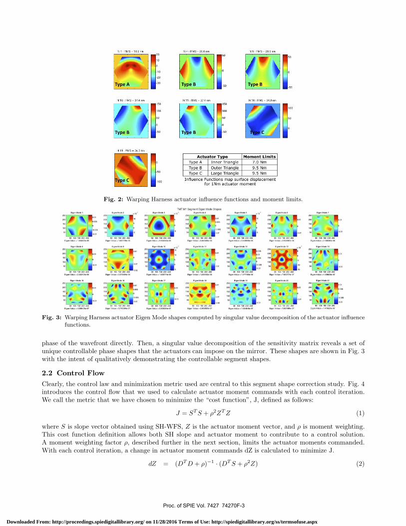
Fig. 2: Warping Harness actuator influence functions and moment limits.

Fig. 3: Warping Harness actuator Eigen Mode shapes computed by singular value decomposition of the actuator influencefunctions.

phase of the wavefront directly. Then, a singular value decomposition of the sensitivity matrix reveals a set ofunique controllable phase shapes that the actuators can impose on the mirror. These shapes are shown in Fig. 3with the intent of qualitatively demonstrating the controllable segment shapes.

2.2 Control FlowClearly, the control law and minimization metric used are central to this segment shape correction study. Fig. 4introduces the control flow that we used to calculate actuator moment commands with each control iteration.We call the metric that we have chosen to minimize the “cost function”, J, defined as follows:

J = ST S + ρ2ZT Z (1)

where S is slope vector obtained using SH-WFS, Z is the actuator moment vector, and ρ is moment weighting.This cost function definition allows both SH slope and actuator moment to contribute to a control solution.A moment weighting factor ρ, described further in the next section, limits the actuator moments commanded.With each control iteration, a change in actuator moment commands dZ is calculated to minimize J.

dZ = (DT D + ρ)−1 · (DT S + ρ2Z) (2)



Fig. 4: Segment shape control flow diagram demonstrating the control flow process followed. The SH-WFS block rep-resents the wavefront sensing model used to estimate the wavefront with each iteration and is defined furtherin Sec. 4.1. As described in Sec. 4.1, this block can be replaced by a phase-based wavefront sensor where thephase is measured directly. Note that if the moment weighting factor ρ is set to zero, that the slope exclusivelyinfluence the minimization the “cost function” J. As a measurement noise, we consider the atmospheric phaseresidual over the segment after integration as described in Sec. 4.2.

where D is the actuator sensitivity matrix. As the controller iterates, the SH slopes are minimized with thepossible consideration of actuator moment, controlled by the moment weighting factor.

The control flow procedure begins with the uncorrected segment surface generated by the process describedin Sec. 3. Treating this surface as the segment wavefront, by assuming no figure errors on the secondary andtertiary mirrors as well as perfect telescope alignment and by including a factor of two (surface to wavefrontconversion assuming normal ray-incidence), we pass this array to the wavefront sensor model. Typically, we usethe SH-WFS described in Sec. 4.1. Here we include the atmospheric phase residual noise, as described in Sec. 4.2with the segment wavefront, divide the segment for each lenslet, and propagate using a Fast Fourier Transform(FFT) to set up the SH spots. A convolution with the time-averaged atmosphere in Optical Transfer Function(OTF) space is then included for each spot. We calculate spot slopes by differencing the aberrated position withthe recorded zero position. As described previously, a set of actuator moment commands is calculated accordingto Eq. (2), that minimizes the J-metric. Using an integrator, these new moment commands are added to thosecalculated from previous iteration and a new wavefront surface is applied using the warping harness influencefunctions. This new corrected wavefront is passed to the wavefront sensor for continued correction.

2.3 Control Parameters

Aside from the SH-WFS design, we have varied two main parameters related to the control law when correctingthe segment surfaces. The first is the number of controlled Singular Value Decomposition (SVD) modes. Whencalculating the control matrix via SVD, we can choose to limit the number of SVD mode shapes to correct. Bydecreasing the number of SVD modes considered in the control matrix, we ignore the mode shapes that havethe weakest control authority. These mode shapes have higher spatial frequency and can increase the actuatormoment commands that achieve the same or very similar surface error after correction. By limiting the includedSVD modes into the control matrix, we can decrease the actuator moment commands and also decrease ourdependence on the accuracy of the D-matrix.

The second main controlled parameter is the actuator moment weighting factor, which controls the amountof consideration given to the actuator moments relative to the slope in the calculation of the J- metric. Thisfactor, called ρ in Eq. (1), is the means of limiting the actuator moments applied in each control iteration. Whenρ = 0, only the slopes are considered when evaluating J. We have found that the actuator moments required to



Fig. 5: Procedure and assumptions for uncorrected segment surface generation. The Noll Zernike polynomial values forthe low order allowances are given in terms of rms values (Zernikes are rms normalized).

correct any given uncorrected segment shape are less than half of their force limits even if ρ = 0. Therefore, weonly consider ρ = 0 throughout this paper.

3. UNCORRECTED SEGMENT SHAPES

3.1 Procedures and Assumptions

The entire surface generation process is outlined in Fig. 5. We generate initial surfaces from a Power SpectralDistribution (PSD) function assuming the following. First, that the PSD amplitude distribution follows theKolmogorov spectrum. Eq. (3) represents the two dimensional Kolmogorov spectrum in unit of phase square perunit spatial frequency area.5

PSD(�f) = 0.023 · r0−5/3 · |f |−11/3 (3)

where �f is the two dimensional spatial frequency, |f | is the magnitude of the spatial frequency, and r0 is theQuasi-Fried’s parameter. Second, the PSD phase distribution follows a uniform probability density functionfrom 0 to 2π (independent and identically distributed). Third, the surfaces are isotropically aberrated, i.e., nodirectional dependencies. We define the segment region to a circular aperture, which encompasses the segmenthexagonal mirror shape, and remove the Piston, Tip, and Tilt (PTT) components afterwards from the surfacedefinition. This initial surface fulfills TMT’s structure function for surfaces having residual polishing errors. Thehexagonal initial segment surfaces are “stamped” out from these initial surfaces.

The TMT mirror specification allows for additional low order aberrations, expressed in terms of circularZernike polynomials, namely: defocus, astigmatism, coma and trefoil. † The permitted Zernike coefficient valuesare listed in Fig. 5. We simply removed the PTT components from these surfaces since telescope alignmenterrors are modeled separately. These uncorrected segment surfaces are fed into the warping harness control flowdescribed in Sec. 2.

3.2 Structure function and Verification of initial surfaces

The structure function defined by the TMT project is the tip/tilt removed atmospheric structure function shownin Eq. (4).

D(x) = A[10.6

(x

d

)5/3

− 13.75(x

d

)2

+ 3.42(x

d

)3]+ B2/2 (4)

†All Zernike modes in this report refer to Zernike Noll Modes5.



0 0.5 10

200

400

600

800

1000

m

nm2

structure function, dx=1/32 [m]

from spec (surface)from D (mean)± σ

(a) sampling dx=1/32 m

0 0.5 10

200

400

600

800

1000

m

nm2



(b) sampling dx=1/64m

0 0.5 10

200

400

600

800

1000

m

nm2



(c) sampling dx=1/128 m

Fig. 6: Comparison between the computed and TMT specified structure functions. The computed structure function isfrom 100 randomly generated initial surfaces (one bounded by dashed lines, blue if colored) using Eq. (5) whilethe TMT specified structure function is from Eq. (4). The calculated structure function is represented by themean value along the radial direction (one bounded by dashed lines, blue if colored) and two dashed line boundsof standard deviations from the mean along the azimuthal direction.

where x is the separation between point pairs, D is the diameter of the telescope, d is the diameter of the beamfootprint, r0 is the Quasi-Fried’s parameter, λ is the wavelength, A = 1/4 × (λ/2π)2 × (D/r0)5/3, and B is thehigh order surface roughness. They are specified as D = 30 m, d = 1.432 m r0 = 1 m, and B = 3.1623 nm for theTMT primary segment mirror. Note that this structure function is described in terms of surface heights and notoptical path differences (OPD). For the following two reasons the white noise component (B) can be ignored:First, we can always separate the white noise term from this study since white noise cannot be corrected bywarping harness. Second, to accurately model a white surface noise would require significantly higher spatialresolution than we currently have.

In order to verify that the initial segment surfaces meet the requirement, we perform Monte-Carlo studies.We first generate many random surfaces and calculate the structure function using Eq. (5).

D(�r) =

∫A(�x)A(�x − �r)

⟨[S(�x) − S(�x − �r)]2

⟩d�x∫

A(�x)A(�x − �r)d�x(5)

where �r and �x are two dimensional spatial coordinate for surfaces, A(�x) is the logical pupil function, S(�x) is thesurface function, and the operator 〈·〉 in Eq. (5) represents the statistic ensemble average of many random trialsof the Monte-Carlo simulation. Eq. (5) is a structure function formula considering a finite pupil. As Eq. (5)suggests, the calculated structure function is defined in two dimensional coordinates. Fig. 6 shows the meanvalue along the radial direction of the calculated structure function from 100 randomly generated initial surfaces(one bounded by dashed lines, blue if colored) and two dashed lines representing bounded standard deviationsfrom the mean along the azimuthal direction. The corresponding structure function that TMT specifies fromEq. (4) (red if colored) is also plotted for comparison. Figures 6(a)–(c) are determined using different grid sizes,i.e., 1/32m, 1/64m and 1/128m respectively.

As seen in Fig. 6, the computed and TMT specified structure functions match reasonably well. Nonetheless,we observe some differences between the two structure functions due to following reasons. One is that high spatialfrequency components are limited by the numerical simulation, i.e., grid size. The other is due to low spatialfrequencies that are limited by surface aperture size. This low frequency limitation results in uncertainty of thepiston, tip, and tilt on the circular aperture over which they are removed after the process. Further investigationon the discrepancy between these two structure functions is beyond the scope of this work. Therefore, we use a1/128 m grid size and this level of surface quality for the remainder of our work. Note that the sample grid sizeof 1/128 m is close to the grid size of the influence functions used in our model and discussed in Sec. 2.

The mean (and standard deviation) of the Root-Mean-Square (RMS) surface for initial (a), initial segment (b),and uncorrected segment (c) surfaces are obtained as 18.4(2.9) nm, 17.3(2.8) nm, and 97.3(7.4) nm, respectively.The results are based on 100 time Monte-Carlo study. The mean RMS surface value of 18.4 nm in initial surfaces



Rings Focal Length (mm) F/# CCD dx (μm)3 45 100.9 154 35 98.0 155 20 67.2 96 20 78.4 9

Table 1: Shack-Hartmann Wavefront Sensor Designs with an example diagram of 3 Ring lenslet configuration sampledover a mirror segment.

(a) can be compared to 19.645 nm, which is obtained using the analytic formula Noll derived.5 The two valuesbeing close to one another suggests that our simulation is valid. The mean RMS surface value of 97.3 nm inuncorrected surfaces (c) can be compared to 115.32 nm, which is Root-Sum-Square (RSS) of the mean valueof initial segment surfaces (17.3 nm) and the RSS value of the low order allowances (114.02 nm) in Fig. 5. Thedifference between the two values is due to the hexagonal shape of the segments. (Higher values of Zernike shapescut out of hexagons.)

4. WAVEFRONT MEASUREMENT

4.1 Wavefront Sensor Models

The most basic wavefront sensor model that we use to estimate the segment shape is a phase-based wavefrontsensor. We refer to this method of estimating the surface shape as the “ideal” wavefront sensor because wesimply use the model’s array representation of the segment as a result of the previous control iteration withno added noise or estimation. This method represents an idealized limit of surface correction obtained only ifthe segment surface shape is entirely known without any noise disturbance. The results shown in the followingsections is a result of using this “ideal” wavefront sensor to minimize the WFE and not its derivative like theSH-WFS’s.

A SH-WFS measures the average wavefront slope over the sampled wavefront defined by an array of lensletspositioned in the pupil-plane. We model the SH-WFS designs that are currently considered by the APS team forperformance evaluation. The basic parameters related to the SH-WFS designs are shown in Tbl. 1. The mainparameter that drives these designs is the number of rings in the lenslet array. Tbl. 1 also shows an examplediagram of 3 Ring lenslet configuration sampled over a mirror segment and describes how the number of ringsis defined. More lenslets give more measurements, a higher sampling, of the wavefront, which increases systemperformance. By considering various SH-WFS designs, we can explore this trade-space to maximize the sensorsystem’s performance while minimizing the cost.

To measure the slopes associated with a certain wavefront shape, the mirror segment is divided up to includethe region that each unique lenslet sees. Using Matlab, we propagate this wavefront for each lenslet via an FFTroutine. Ideally, the spot resulting from this propagation is then stitched into an array corresponding to thedetector and sampled over its designed pixel size. When a perfect wavefront is propagated through the lensletarray, each spot has zero motion. However, when the sensor samples a disturbed wavefront, the tip and tilt ofthe spot creates a slope measured by the sensor and provides an input to the control algorithm described in thissection.

As an approximation to this SH-WFS model, a simplified centroiding algorithm is used. The centroid of thelenslet spot is the measured position of the spot’s peak on the detector. Much effort can be contributed to thealgorithm used for this spot centroiding. We have used the most basic method for finding the peak, by ignoringthe effects of neighboring spot diffraction crosstalk. We also have increased the detector sampling and positionedthe detector such that the spot peak is always aligned with a specific pixel. This avoids some complexity in thewavefront sensor model and does not consider some approximation in the spot location. Future work can increasethe maturity of this method. An advance spot centroiding routine will account for these approximations.



Moment Limit Ratio RMS WFE [nm] PSSNWavefront 21 SVD 10 SVD 21 SVD 10 SVD 21 SVD 10 SVD

Sensor Modes Modes Modes Modes Modes ModesIdeal 0.31 0.18 20.64 24.65 0.9557 0.9441

SH 3-Ring 0.40 0.25 22.10 25.41 0.9499 0.9420SH 4-Ring 0.45 0.25 21.66 25.33 0.9532 0.9446SH 5-Ring 0.35 0.21 21.16 25.05 0.9555 0.9465SH 6-Ring 0.34 0.21 21.15 25.23 0.9562 0.9469

Table 2: TMT Segment Shape Control Study

4.2 Measurement Noise

Possible measurement noise sources in the SH-WFS include centroid spot uncertainty and Atmospheric PhaseResidual Noise. The centroid spot uncertainty is the uncertainty in finding correct slopes in SH-WFS, whichresults from various different error sources such as non-perfect centroid algorithm, spot broadening effect inducedby atmosphere, finite detector pixel size, and aberration in the lens arrays. The “Atmospheric Phase ResidualNoise” is due to finite exposure time through the random atmosphere. Chanan, et al.6 have found that the“Atmospheric Phase Residual Noise” is the most dominant error source in the Phasing Camera System (PCS)7 ofthe Keck Telescopes. They have also predicted the (atmospheric residual dominant) measurement uncertaintiesof the Alignment and Phasing System (APS) based upon empirical data from PCS, scaling them as appropriateto TMT. The APS of TMT is responsible for the precision optical alignment of the telescope.8

In this study, we implement these APS measurement uncertainties in the form of measured segment wavefrontuncertainties, expressed via Zernike polynomials, representing additional segment aberrations due to atmosphericintegration. The Zernikes included are: focus, astigmatism, coma, and trefoil, which are scaled as a functionof the integration time that APS measures over. Since a longer integration time reduces this estimation error,we model the current minimum time allowed by the APS requirements of ΔT=300 seconds so that we do notunderestimate its affect. We add a randomly composed segment Zernike array, scaled by this integration time,to the wavefront disturbance present on the mirror segment as a result of each control iteration.

We refer to this noise as “Atmospheric Phase Residual Noise” since the APS uncertainties mainly come fromthe atmosphere phase residual or simply “APS Noise” throughout this paper.

5. SIMULATION RESULTS

We present our simulation results in terms of the PSSN1, 3 metric in this section. The following is a list ofassumptions and approximations that we have made during the implementation of our optical TMT model.3

First we assume that the primary mirror is made up of a regular hexagon grid. This means that our primarysegments each have the same regular hexagonal shape in projection. Our OPD map exit pupil sampling is1/64 m per pixel. Also each mirror surface deformation is approximated using a regularly sampled grid. In thissimulation, the primary mirror segments each use a 256 × 256 pixel grid with 5.6 mm pixels.

Our default simulation parameters include a wavelength of 500 m and atmospheric r0 equal to 200 mm at thezenith. Currently, we have run cases for SH-WFS 3-6 ring designs in addition to the “ideal” phase based sensordescribed in Sec. 4. For SH-WFS, we employ the simplified centroid algorithm as described in Sec. 4.1. We havesimulated the SVD mode control of 10 and 21 modes, with ρ = 0. For all cases, we currently include the APSnoise described in Sec. 4 (including the approximations as described in Sec. 4.1), with a 300 sec integration time.

To calculate PSSN values for each set of control parameters, we begin with a database of 492 correctedsegments. We then load each of these segment grids, ensuring that they are correctly sampled and have piston,tip, and tilt removed. Each segment grid is installed into the TMT MACOS optical model’s primary mirror. AnOptical Path Difference (OPD) map is defined by a sequential ray-trace and we calculate the PSSN for each case.Table 2 contains results for each of the control parameters listed above, which are also shown in Figs. 7(a)-7(b).

Tbl. 2 shows simulation results from this warping harness correction study. Overall, there is a minimalchange in its value from the April-2008 Performance Review3 estimate of 0.9494 for r0 = 200 mm at Zenith.



(a) (b)

Fig. 7: Example case study where a wavefront correction algorithm is applied to correct an uncorrected segment shape.For this specific case study, we assume SH-WFS design, controlled SVD modes, moment weighting of 3-Ring, full21 modes, and 0, respectively. For each iteration step, interesting properties such as the metric (c), the RMSWFE (d), and actual actuator moments (e) are shown.

By including higher spatial frequencies and shortening the APS integration time, the PSSN value is lowered.This decrease in the PSSN is counteracted by an improvement in the warping harness correction method. Theseimprovements include using the designed influence functions and actuator moment limits as described in Sec. 2.The “ideal” phase-based wavefront sensor minimizes the RMS WFE relative to the SH WFS designs. It isinteresting to note that although this phase-sensing method minimizes the wavefront error, the PSSN value isminimized using the slope-based approach. Using the 5- or 6-ring SH-WFS design, with the first 10 SVD modescontrolled, optimizes the RMS WFE and PSSN values. The effects of including high frequency errors througha PSD surface implementation and an improvement in the warping harness surface correction nearly cancel oneanother in terms of PSSN, resulting in only a small overall change since the TMT Performance Review in April2008.

6. SUMMARY

Based on our assumptions and models of the primary segment residual errors, we have estimated that the PSSNis 0.9499 using our baseline parameters, i.e., 3-ring SH-WFS, 300 sec APS integration time, no moment weighting(no restrictions upon actuator movements applied) and utilizing all 21 SVD modes for the WFE control. Wehave also observed the possibility to improve this PSSN value to 0.9555 (5-ring SH-WFS) or 0.9562 (6-ring SH-WFS). We estimate that the RMS WFE due to uncorrected segment shape is less than 100 nm before correctionand reduces to less than ≈ 22 nm after correction. The updated PSSN value of 0.9499 is close to what wehave reported previously using the simple Zernike model.3 Although we have an improved surface model thatbetter represents the assumed polishing errors (representation of higher spatial frequencies), the enhanced controlalgorithm permits a better WFE correction over the segments. A detailed summary of the obtained results ispresented in Tbl. 2 in Sec. 5.

In addition to these PSSN metric updates, we have made the following observations : First, our simulationsindicate that, for the provided input specifications, the maximum observed actuator moment is 60% of the limit.This result was achieved without utilizing the actuator moment weighting factor in the control algorithm or bylimiting the number of controlled SVD modes; two methods that could further reduce these commands. Second,we investigated the WFE correctability using the available range of 1 to 21 SVD modes. If the control is limitedto include only the 10 largest SVD modes, i.e., not including higher spatial frequency modes, we observed thatthe moments applied to the actuators is reduced by 50% and that the difference of the RMS WFE values wasabout 5 nm. Using only the strongest 10 SVD modes makes the control more robust. Third, as to be expected,we confirmed that the 5- or 6-ring SH-WFS designs considered by the APS team outperform the 3-ring SH-WFS



design. We observed that these finer sampled wavefront sensors increase the PSSN ≈0.0056 and reduce the RMSWFE by ≈1 nm. Although we have not observed a significant difference between the 5- and 6-ring lenslet array,a more careful study is suggested to investigate the trade-off space between them.

ACKNOWLEDGMENTS

This research was carried out in part at the Jet Propulsion Laboratory, California Institute of Technology, andwas sponsored by the California Institute of Technology and the National Aeronautics and Space Administration.The authors gratefully acknowledge the support of the TMT partner institutions. They are the Association ofCanadian Universities for Research in Astronomy (ACURA), the California Institute of Technology and theUniversity of California. This work was supported as well by the Gordon and Betty Moore Foundation, theCanada Foundation for Innovation, the Ontario Ministry of Research and Innovation, the National ResearchCouncil of Canada, the Natural Sciences and Engineering Research Council of Canada, the British ColumbiaKnowledge Development Fund, the Association of Universities for Research in Astronomy (AURA) and the U.S.National Science Foundation.

REFERENCES

1. B.-J. Seo, C. Nissly, G. Angeli, B. Ellerbroek, J. Nelson, N. Sigrist, and M. Troy, “Analysis of Normal-ized Point Source Sensitivity as a performance metric for the Thirty Meter Telescope,” Proc. SPIE 7017,p. 70170T, June 2008.

2. G. Z. Angeli, S. Roberts, and K. Vogiatzis, “Systems Engineering for the Preliminary Design of the ThirtyMeter Telescope,” Proc. SPIE 7017, p. 701704, June 2008.

3. C. Nissly, B. Seo, M. Troy, G. Angeli, J. Angione, I. Crossfield, B. Ellerbroek, L. Gilles, and N. Sigrist,“High-resolution optical modeling of the Thirty Meter Telescope for systematic performance trades,” Proc.SPIE 7017, p. 70170U, June 2008.

4. E. Williams, C. Baffes, T. Mast, J. Nelson, B. Platt, R. P. E. Ponslet, S. Setoodeh, M. Sirota, V. Stephens,L. Stepp, and A. Tubb, “Advancement of the segment support system for the thirty meter telescope primarymirror,” Proc. SPIE 7018, p. 701810, June 2008.

5. R. J. Noll, “Zernike polynomials and atmospheric turbulence,” J. Opt. Soc. Am. 66, p. 207, 1976.6. G. Chanan, M. Troy, and I. Crossfield, “Predicted measurement accuracy of the TMT Alignment and Phasing

System,” TMT Project Communication TMT.CTR.PRE.07.007.REL01, Feb 2007.7. G. Chanan, “Design of the Keck Observatory alignment camera,” Proc. SPIE 1036, p. 59, 1988.8. J. E. Nelson and G. H. Sanders, “TMT Status Report,” Proc. SPIE 6267(626728), 2006.



investigation of primary mirror segment's residual errors...

Documents